ECON60022 Development Microeconomics

Lectures 6 & Tutorial 4: ‘Models on Rural Credit Markets’

Katsushi Imai Email: katsushi.imai@manchester.ac.uk

Office Hours: Tuesday 3.30-5.30

2

0. Schedule Lecture 6 Rural Credit Markets 12 March

Based on Chap. 7 B & U (Tutorial 4 --Lec.6) 17 March Lecture 7 Microfinace 19 March

Based on Ahlin and Townsend (2007) (Tutorial 5 –Lec.7) 24 March Lecture 8 Savings, & Risk, Insurance 26

March -Mock Exam Sheet provided

-Mainly based on Chap. 8 B & U & Deaton (1991)

(Easter Break)

3

Lecture 9 Poverty & Vulnerability 30 April

Hand in your answers

-Mainly based on Ligon and Schechter (2003) and

-Hoddinott and Quisumbing (2003) (Tutorial 6) 5 May A

session for the Mock Exam Lecture 10 Institution and Social Capital – Role of

State 12 May -Mainly based on Chap. 17 B & U.

4

1. Introduction

(a) Dependency of agricultural sector in many LDCs (see Lecture 1)

(1)The lag between the start of production & the realization of agricultural output- Seasonality.

(2) External shocks (e.g. weather- drought/ floods), price shocks, global financial crisis.

(3) Potential mechanisms for these: Savings, Insurance (Lecture 8) or Credit.

World Bank ,2000, World Development Report 2000/01: Attacking Poverty, Washington D.C

Alderman and Paxson, 1994, Do the poor insure? A synthesis of the literature on risk and consumption in developing countries.

5

(4) Savings may not possible for the poor. Formal insurance schemes are limited.

(b) The credit is often limited, particularly, for the poor.

(1) Formal credit (e.g. banks or cooperatives) is limited.

(2) Informal credit (credit not from formal sectors- incl. borrowing from money lenders microcredit from small NGOs, credit from relatives & friends or from employers) important.

(3) A type / terms of loans vary (duration, with/ without collateral/ interest rate/ group or individual liability) to a great deal.

6

(c) Roles of government policies

(1) Governmental Policies are important (whether to impose interest rate ceilings/ whether to target particular sectors/ type of business/ whether to opt for subsidized credit programmes). Risky nature of the agricultural production.

(2) Efficiency vs. Equity Whether the government should liberalise the credit market?

 

7

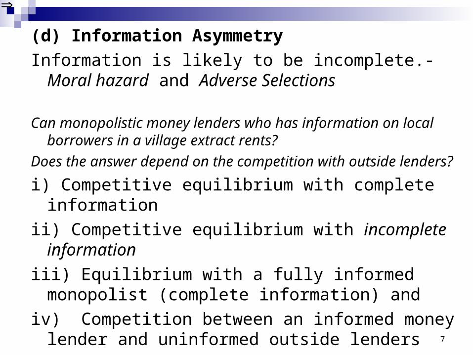
(d) Information Asymmetry

Information is likely to be incomplete.-Moral hazard and Adverse Selections

Can monopolistic money lenders who has information on local borrowers in a village extract rents?

Does the answer depend on the competition with outside lenders?

i) Competitive equilibrium with complete information

ii) Competitive equilibrium with incomplete information

iii) Equilibrium with a fully informed monopolist (complete information) and

iv) Competition between an informed money lender and uninformed outside lenders  

8

1. Models(a) Assumptions- See handout.

Prob. Borrower Lender Success π(a) R- i - D(a) i Failure 1-π(a) - D(a) 0

The expected utility of a borrower: The expected utility of a lender:

Moral Hazard (Bardhan & Udry, p.80)

i) Competitive equilibrium with complete information

Assumptions:

Large no. of competitive lenders.

Lenders can observe the borrower’s choice of a (an index of the farmer effort) and the interest factor, i, and can write contracts that specify i and a.

9

An equilibrium 11 a,i is defined such that it satisfies the following conditions.

a. Wa,iU 11

b. 111 a,iUi

c. There is no other pair that yields a return greater than or equal to

to a lender and which a borrower would prefer to 11 a,i .

10

aDiRaMaxa,i

(1)

s.t. ia (2)

and .WaDiRa (3)

If there is an equilibrium with lending, it is characterized by the solution to:

COSTMARGINAL1

RETURN MARGINAL1 a'DRa' (4)

WaDRa

aDa

RaaDiRaa,iU

11

11

111111

(3)”

ii-1) Competitive equilibrium and moral hazard

Assumptions:

Large no. of competitive lenders (same as i).

Lenders can not observe the borrower’s choice of a. (an index of the farmer effort) .

The borrower will choose the action that maximizes his utility given the credit contract offered.

11

An equilibrium is defined such that it satisfies the same conditions, plus

The lender can only offer contracts such that the borrower wants to choose a2, given i2.

If there is an equilibrium with lending, it is characterized by the solution to:

12

aDiRaMaxa,i

(1)

s.t. ia (2)

.WaDiRa (3)

and 1,0aaDiRaaDiRa (5)

or 1,0aa,iEUa,iEU

ii)-2 Competitive equilibrium and moral hazard (with collateral)

Assumptions Large no. of competitive lenders Lenders can not observe the borrower’s choice of a

(an index of the farmer effort) . The borrower will choose the action that maximizes

his utility given the credit contract offered. Borrowers and lenders are risk neutral. Each borrower owns some asset > R. If the project fails, the borrower transfers the

collateral to pledged for the loan (C) to the lender. 13

Then the equilibrium, if it exists, is described by

14

CaaDiRaMaxC,a,i

1 (8)

s.t. Ca1ia (9)

.WaDCa1iRa (10) and 1,0aaDCa1iRaaDCa1iRa

or 1,0aa,iEUa,iEU (11)

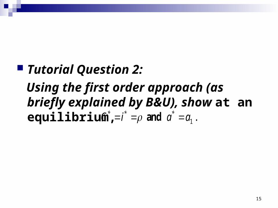
Tutorial Question 2:

Using the first order approach (as briefly explained by B&U), show at an equilibrium,

15

** iC and 1aa* .

the problem of moral hazard will be completely alleviated in case with collateral (NB- if the farmer makes more effort, the risk of collateral C being taken will be reduced).

Implications:

-This will explain the lender’s preference for taking collateral and for the relatively rich borrowers who can afford collateral, land. -The poor households cannot have access the lending.

16

The collaterals can be transacted in the secondary market. Also, the collaterals should be free from information problems (e.g. if people realize the risk of giving their collateral (e.g. livestock) to the lender, they may not try to take care of it well).

17

This will justify the group lending without for borrowers without physical collateral (Lecture 7) –joint liability

In some areas of LDCs, the labour market contract is linked with the credit contract (interlinked transaction).

18

The results depend on the assumption that both borrowers and lenders are risk neutral. If the borrowers are risk-averse, the difficulties with moral hazard will not be alleviated totally as they will not be willing to take entire the risk without some compensation from the lender.

19

iii) Equilibrium with a fully informed monopolist

Assumptions: There is only one local money lender whose

wealth is larger than the total wealth of N residents in the village).

The money lender can monitor the activities of borrowers (hence a, an effort level).

The opportunity cost of wealth is the risk-free rate, rho (the opportunity cost).

20

Because of the monopoly, zero profit constraint will be relaxed. The moneylender can actually maximize

The interest rate is set so that the lender maximizes his expected return and the borrower achieves the reservation utility.

21

iaMaxa,i

(16)

s.t. WaDiRa (17)

and .ia (18)

COSTMARGINAL

3RETURN MARGINAL

3 a'DRa' (19)

iv) Competition between an informed money lender and uninformed outside lenders Assumptions: There is a competitive market for credit from

lenders outside the village without the knowledge of borrower’s activities.

As in case iii) there is a local moneylender in the village who can monitor the activities of farmers without any cost.

The opportunity cost for those lenders is rho The opportunity cost for local money lender is

the risk-free rate, rho (the opportunity cost).

22

23

If the outside lenders enter into the village market (competitively), the reservation wage will rise to W2..

Then the local moneylender implements the contract based on W2..

The local moneylender will obtain the positive profit ( 　

221144iaiaia ) to reflect

their advantageous position.

24

Tutorial Question 1: Show that the curve for

iaa,i is downward-sloping and strictly convex (p.4 in the hand out)

a

i

(2)’

0a

a'dadi

2

*1

0a

a'aa

dad

dadi

2

21

Intuition- At any point satisfying (2)’, if the lender increases a by a small amount in the contract, a , the probability of successful crop, will increase. So i has to be reduced.

25

Strictly convex: 2

aa'

dadi

02

22

4

2

NEGATIVE

POSITIVEPOSITIVEPOSITIVENEGATIVE

aaaaada

id

*2 NB: This is based on ‘Quotient Rule’

xg

x'gxfxgxf

xg

xf

dx

d2

Intuition- At any point satisfying (2)’, if the lender increases a by a small amount in the contract, then a , a marginal increase in the probability of successful crop, will decrease (because of the concavity of a ). Marginal decrease in (di) corresponding to the marginal increase in a (da) will decrease for larger a.

26

Tutorial Question 2: Using the first order approach (as briefly explained by B&U), show at an equilibrium,

** iC and 1

* aa . (moral hazard with collateral).

Ca1aDiRaMaxC,a,i

(8)

s.t. Ca1ia (9) .WaDCa1iRa (10) & 1,0aaDCa1iRaaDCa1iRa

or 1,0aa,iEUa,iEU (11) Using the first order approach, the last constraint (11) can be replaced by the FOC for the borrower- 0aDCiRaaDCaiRa (12)

27

Because the lender earns no profit under the perfect competition, from (9) we get Ca1ia (13)

From (13) we get

Ca

Ci

(13)’

By substituting (13)’ into (12) 0aDCiRaaDCaiRa (12)

we will get

0aDa

CRa

Solving this for C we will get

aDa

aRaC

(14)

Substituting (14) into (13)’

CaD

a

aRa

a

1i

Ra1aDa

a1

(13)”

28

Substituting these (i and C) into the objective function (8),

Ca1aDiRaMaxC,a,i

aDa

aRaa1

aDRa1aDa

a1RaMax

a

aDRaMaxa

F.O.C. is ** aDRa . (15) This is same as the optimal solution for the case i) competitive equilibrium with complete information, the equation (4). The borrower’s effort at equilibrium *a is

1

* aa .

29

If we use (15), we can show that from (14):

aDa

aRaC

(14)

Raa

aRaC **

From (15) and (13)” :

Ra1aDaa1

i

(13)”

Ra1Ra

a

a1*i

Adverse Selection

30

Assumptions: -Farming requires no effort. -There are two types of potential borrowers indexed by .2,1t -Type 2 has access to land (or crop) that is riskier but more lucrative (high risk & high return). – ‘Riskier’ farmer. -Type 1 has access to land (or crop) that is safer but less lucrative (low risk & low return). –‘Safer’ farmer.

31

- 21 where t is a probability of successful farming for Type t. - 2R1R where tR is a return of successful farming for Type t.

1. The expected return to farming each type of land is identical.

tRtRt 2. The reservation utility of the

different types of the borrower (e.g. wages in the non-farm sector).

tWtW

32

As before, the expected utility of borrower is itRtt,iU The expected return from a loan at rate i to a type t borrower is itt,i

i) Competitive equilibrium with complete information Assumptions:

-Large no. of competitive lenders.

-Lenders can observe the borrower’s type t and can offer different factors, i.

33

34

An equilibrium with lending to the type t, ti

1 is defined such that it satisfies the

following conditions. a. Wt,tiU

1

b. t,ti1

c. There is no interest rate ti that yields

a return greater than or equal to and which a type t borrower would prefer to ti

1.

35

If there is an equilibrium with lending, it is characterized by the solution to:

titRtMax

ti (20)

s.t. tit (21) and .WtitRt (22) If WR , (23) there will be lending in equilibrium to both types. Otherwise neither type will receive loans.

Both type of farmers will borrow.

ii)-1 Competitive equilibrium with adverse selection

Assumptions:

Large no. of competitive lenders (same as before).

Lenders can not observe the borrower’s type t.

Lenders know the relative proportion of Type 1 and Type 2.

36

37

At any given interest rate i, i1Ri1R11,iU i2Ri1R22,iU Because 21 , 2,iU1,iU That is, ‘high-risk high-return’ borrower (Type 2) will get the higher expected utility than the ‘low-risk low- return borrower (Type 1) given an interest rate i.

38

However, 2,ii2i11,i That is, at a given interest rate i, the expected return from a loan to Type 1 is larger than that from Type 2. As before, the expected utility of borrower is: titRtt,tiU

1

0t

i

itRt

i

t,iU

39

Here we define 1i * as the highest interest rate at which Type 1 borrowers are willing to borrow. W1i1R1i1R1 **

Hence 1WR

1i *

Similar;y, 2

WR2i *

Because 21 , 2i1i ** .

40

The Implications As the interest goes up, Type 1 (safer)

borrowers will drop out and opt for the non-farm employment without any risk.

Figure 7.2 will illustrate the relationship of interest rate charged by lenders, i, and the expected income from the lending

41

Suppose 1p is the proportion of the population of potential borrowers who are Type 1 (safer borrower). 11p0 Case 1 1ii0 *

i21p1i11piE (24) 021p111p

di

)iE(d

Case 2 2ii1i * Type 1 borrowers now choose the risk-less non-farm employment. So the lenders income will fall suddenly from 1i21p11i11p ** to

1i21i21p1 ** as p(1) becomes 0.

42

i2iE (25)

02

di

)iE(d

Because 21 >0 the slope is positive but less steep. The competitive equilibrium with adverse selection is defined as an interest rate

2i :

(a) 2

iE That is, a lender on average do not lose the money at 2i (earn the profit which is positive or equal to 0).

(b) There is no interest rate i for which: i. iE

ii. t,iUt,iU2

& Wt,iU

43

That is, there is no other levels of interest i, at which any Type t borrower would take the loan and would be better off than the utility level achieved under (and the lender still makes a profit greater than 0).

As long as WR (same as (23)), there will be lending in the equilibrium with adverse selection.

44

If 1i21p11i11p1iE **"

(26) Then, from (25)

22i2iE

Then the equilibrium interest rate is

i

2i

2

(Figure 7.2).

----------Only the ‘high-risk high-return’ borrower will demand loans.

45

However, if 1i21p11i11p1iE **"

Then, from (24)

222i21p1i11piE

(27) Then, the interest rate will be 1i21p111pi *

2

(27)’ Then all the borrowers will demand loans. At i

~ , only the ‘high-risk high-return’ borrowers will demand the loan, but it is not an equilibrium as all the borrowers prefer

2i to i

~ (see Figure 7.3).

ii)-2 Implications of Adverse selection- Credit Rationing

We have so far assumed that lenders have access to an infinitely elastic supply of funds at rho.

Stiglitz and Weiss (1981)

- When the relationship between the expected return to lenders and the interest rate is not monotonic with an interior local maximum, there exists a supply of fund schedule which leads to a competitive equilibrium with credit rationing 46

ii)-3 Competitive equilibrium and adverse selection (with collateral)

The existence of collateral can eliminate the problem of adverse selection (a pledge of collateral equals to the repayment places the entire risk of the transaction on the borrower).

  The results depend on the risk-neutrality of

the borrower.

47

iii) Equilibrium with a fully informed monopolist

48

Moneylender’s problem is to set an interest rate ti

3 for the type t borrower.

His going to maximize his expected return from his lending by solving:

titMax

ti (28)

s.t. WtitRt (29) and .tit (30)

49

If WR , (31) the lending at equilibrium is with .ti

3 in

case there is lending. As (29) binds with equality (because of the ability of money lender to observe the type), WtitRt

3

tit

WRti *

3

(32)

-Each type of borrowers achieves an expected utility of W (minimum level with an incentive to borrow). -the lender earns:

WR

t

WRttit

3

iv) Equilibrium with a fully informed monopolist(and with competitive outside lenders)

50

Case 1 (corresponding to Figure 7.2) WR1iE *

The equilibrium with competitive, uninformed lenders ----Lending only to Type 2 lenders Interest rate with this lending 2it (because of the zero profit condition).

2

2i

51

Suppose we denote the interest rate charged by the local lender is ti

4.

He will charge 2

2i4

for the Type 2

borrowers. He can charge (as in (32))

1

WR1i

4

52

Case 2 (corresponding to Figure 7.3) 1iE *

The equilibrium with competitive, uninformed lenders ----Lending only to Type 1 & Type 2. -Local lender knows the type of lenders, while the outside lenders do not. -The equilibrium with the competitive uninformed lenders. -Lending to both types of borrowers ( 1ii *

2 for Type 1 and i

~ for Type 2)

53

54

However, the local lender can set the interest rate 1i

4 just below

2i and would

attract some of all Type 1 lenders. Hence, the outsider lenders cannot lend Type 1 as their expected return will be below . -Outsider lenders will lend only to Type 2 borrowers at i

~ . The local lenders will also lend to Type 1 lenders at i

~ . The local money lender will earn his rents on his rents to Type 1 is (from (27)’) 21p111p21p111p1i11i1

24

55

However, if 1i21p11i11p1iE **"

Then, from (24)

222i21p1i11piE (27)

Then, the interest rate will be 1i21p111pi *

2

Then all the borrowers will demand loans. At i

~ , only the ‘high-risk high-return’ borrowers will demand the loan, but it is not an equilibrium as all the borrowers prefer

2i to i

~ (see Figure 7.3).

Conclusions

We have seen by the static models Information Asymmetries may lead to

the inefficient allocation of credit or to excessive loan default as a consequence of moral hazard.

They may lead to monopoly profits of local money lenders with the knowledge of local borrowers.  

Collateral will mitigate the problems.

56