Econ 551 Government Finance: Revenues Winter 2018faculty.arts.ubc.ca/kmilligan/teaching/ECON551/551-slides-10.pdf · Government Finance: Revenues ... Oates and ‘fiscal federalism

ECON 551: Lecture 10 1 of 39

Econ 551

Government Finance: Revenues

Winter 2018

Given by Kevin Milligan

Vancouver School of Economics

University of British Columbia

Lecture 10: Federalism and Intergovernmental Grants


Agenda

1. Overview

2. Models of Federalism: Breton + Oates.

3. Intergovernmental Grants

4. Equalization Grants


Overview of Federalism

What should be the relationship between national and subnational jurisdictions?

• Should there even be subnational jurisdictions?

• How many? Three big ones? Many little ones?

How would a non-economist motivate subnational jurisdictions?

• Allows political liberty and cultural autonomy. Schools, church, language. Think of

Switzerland, Canada, Germany.

• Fosters political participation


Economic Motivations for Federalism

Local Public Goods: the MES for public goods might be small.

Spillovers: The extent and nature of spillovers among regions

Laboratory: Justice Brandeis in New State Ice Co. V. Liebman 285 US 262, 311 (1932).

“It is one of the happy incidents of the federal system that a

single courageous state may, if its citizens choose, serve as a

laboratory; and try novel social and economic experiments

without risk to the rest of the country.”


In 1926, the shares were: 37.8 fed, 20.2 prov, 42.0 local. (Source: Musgrave, Musgrave, and Bird)




Agenda

1. Overview





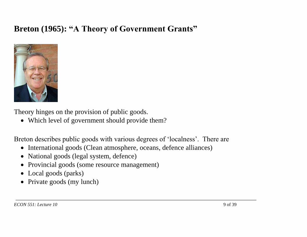
Breton (1965): “A Theory of Government Grants”

Theory hinges on the provision of public goods.

• Which level of government should provide them?

Breton describes public goods with various degrees of ‘localness’. There are

• International goods (Clean atmosphere, oceans, defence alliances)

• National goods (legal system, defence)

• Provincial goods (some resource management)

• Local goods (parks)

• Private goods (my lunch)


Breton (1965): “A Theory of Government Grants”

In a world like this, Breton describes the ‘optimum constitution.’

• All objective benefits of the local good are exhausted

within the border of the jurisdiction.

• Provides a ‘perfect mapping’ between the scope of local

public goods and the political jurisdiction.

• This generalizes the Tiebout idea to vertical levels of goods.

• With lump-sum or benefit taxes, we get Pareto optimal allocations.

• OR, with a supra level of government, they could make conditional grants to ensure that each

level can pay for its optimal level of goods.


Solutions to inter-jurisdictional externality problem

How can we solve this externality problem? Try central government.

• Could be direct provision by feds.

• Could be quantity control through regulations or conditional grants.

• Could be price control through subsidies / matching grants.

Could we just let Coasian bargaining solve the inter-jurisdictional problem?

• Translink presumably accounts for city-to-city spillovers. Garbage

collection and fire stations, however, are done locally. If there are spillovers,

then they made a deal to account for them in that area alone but not for all

goods.

• But, bargaining problems: uncertain property rights, uncertainty about

others’ threat points, free-riding by jurisdictions, enforceability of

agreements—governments might renege.


Oates and ‘fiscal federalism’

The seminal work in this area is a book by Wallace Oates called Fiscal Federalism (1972).

• The model laid out in the book studies the costs and benefits of decentralization.

Local Governments:

• Can respond to local tastes and preferences.

• Cannot produce public goods efficiently if MES is large, or spillovers

exist.

Central Governments:

• Can deal with externalities and scale.

• But cannot respond to local tastes—assumption of “policy

uniformity.”


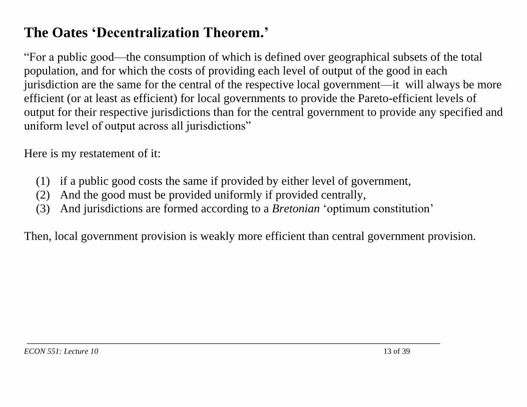
The Oates ‘Decentralization Theorem.’

“For a public good—the consumption of which is defined over geographical subsets of the total

population, and for which the costs of providing each level of output of the good in each

jurisdiction are the same for the central of the respective local government—it will always be more

efficient (or at least as efficient) for local governments to provide the Pareto-efficient levels of

output for their respective jurisdictions than for the central government to provide any specified and

uniform level of output across all jurisdictions”

Here is my restatement of it:

(1) if a public good costs the same if provided by either level of government,

(2) And the good must be provided uniformly if provided centrally,

(3) And jurisdictions are formed according to a Bretonian ‘optimum constitution’

Then, local government provision is weakly more efficient than central government provision.


The Oates ‘Decentralization Theorem.’

The central tension is between policy uniformity and externalities.

• If no externalities, then local provision is weakly preferred.

• If all had same tastes, then central provision is weakly preferred.

• Optimal division is found at the point where the cost of policy uniformity equals the gain from

internalizing the externalities.

Think of this in a two-by-two box:

Same tastes Different tastes

Spillovers Centralization Tension

No spillovers Either / or Decentralization


Agenda

1. Overview





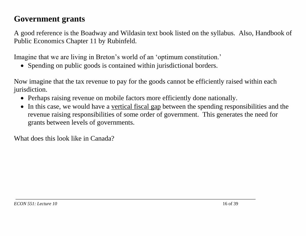
Government grants

A good reference is the Boadway and Wildasin text book listed on the syllabus. Also, Handbook of

Public Economics Chapter 11 by Rubinfeld.

Imagine that we are living in Breton’s world of an ‘optimum constitution.’

• Spending on public goods is contained within jurisdictional borders.

Now imagine that the tax revenue to pay for the goods cannot be efficiently raised within each

jurisdiction.

• Perhaps raising revenue on mobile factors more efficiently done nationally.

• In this case, we would have a vertical fiscal gap between the spending responsibilities and the

revenue raising responsibilities of some order of government. This generates the need for

grants between levels of governments.

What does this look like in Canada?



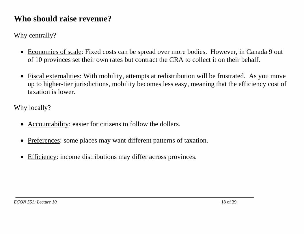
Who should raise revenue?

Why centrally?

• Economies of scale: Fixed costs can be spread over more bodies. However, in Canada 9 out

of 10 provinces set their own rates but contract the CRA to collect it on their behalf.

• Fiscal externalities: With mobility, attempts at redistribution will be frustrated. As you move

up to higher-tier jurisdictions, mobility becomes less easy, meaning that the efficiency cost of

taxation is lower.

Why locally?

• Accountability: easier for citizens to follow the dollars.

• Preferences: some places may want different patterns of taxation.

• Efficiency: income distributions may differ across provinces.


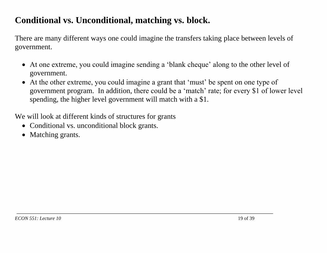
Conditional vs. Unconditional, matching vs. block.

There are many different ways one could imagine the transfers taking place between levels of

government.

• At one extreme, you could imagine sending a ‘blank cheque’ along to the other level of

government.

• At the other extreme, you could imagine a grant that ‘must’ be spent on one type of

government program. In addition, there could be a ‘match’ rate; for every $1 of lower level

spending, the higher level government will match with a $1.

We will look at different kinds of structures for grants

• Conditional vs. unconditional block grants.

• Matching grants.


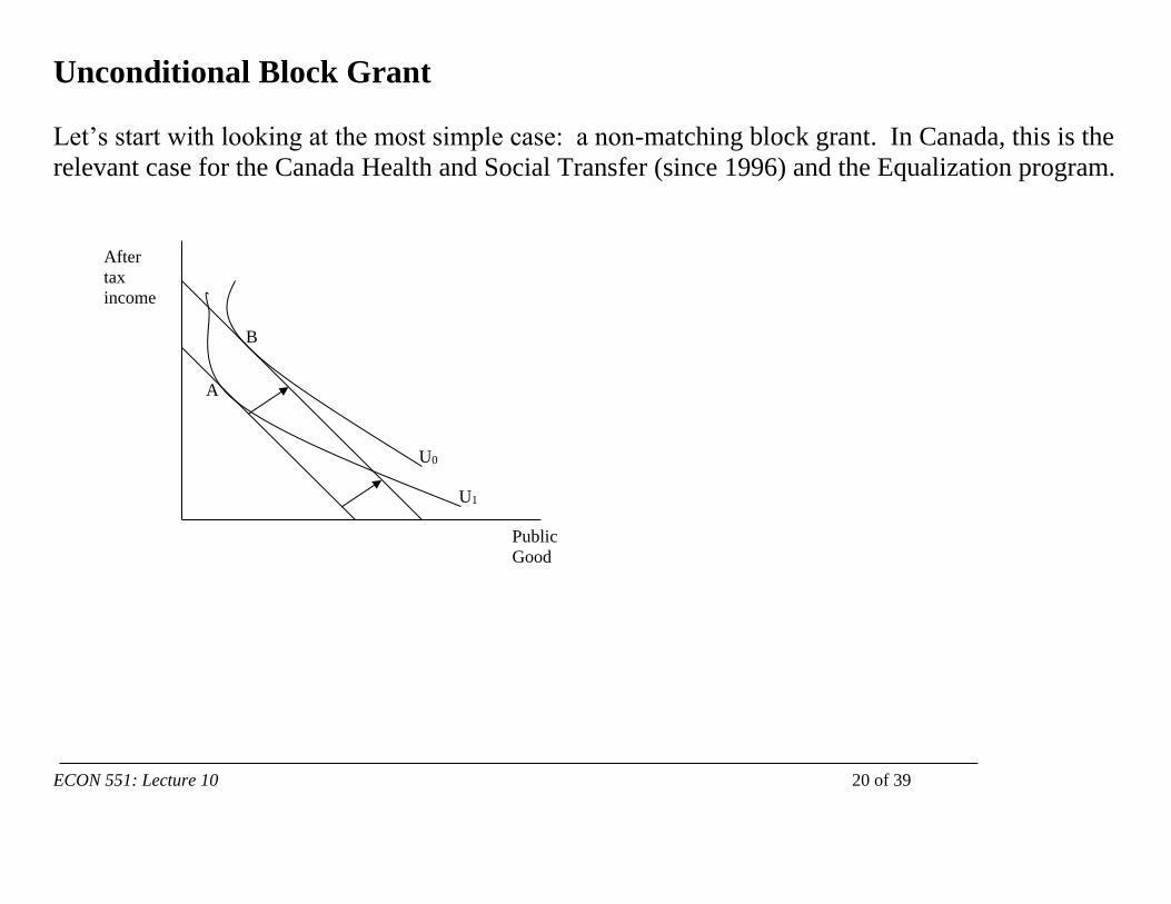
Unconditional Block Grant

Let’s start with looking at the most simple case: a non-matching block grant. In Canada, this is the

relevant case for the Canada Health and Social Transfer (since 1996) and the Equalization program.

After

tax

income

Public

Good

U0

U1

A

B


Unconditional Block Grant

The graph shows:

• After tax income of the province on the vertical axis. (This could equivalently be thought of

as amount of the private good.)

• Spending on the public good on the horizontal axis.

• ‘Community Indifference Curves’ representing the ‘province manager’ or the median voter.

• The effect of the block grant is to move the budget constraint out in a parallel way.

• The equilibrium moves from A to B.

• Point B could be to the left or to the right of point A, so that the block grant could lead to

higher or lower public good spending. It depends if the public good is normal or inferior.

Bradford and Oates (1971) show that grants should almost completely crowd out local government

spending, because the median voter takes the grant as an increase of income. The MPC on local

public goods is likely only around 5%, so we shouldn’t expect a large increase in spending.


Flypaper effect

How much do grants increase spending? Do they ‘stick’ where they land?

What are some explanations for this phenomenon?

• Econometric explanation: Unobserved variables. High spending states might attract more

grants.

• Fiscal Illusion: The spending decisions depend on the source and perceptions by voters of the

revenue. Grants are not a ‘veil’ for a federal tax cut. This might occur if voters are

imperfectly informed, and/or bureaucrats try to maximize the size of their bureaus. (Niskanen

1971)

Counterexample: late 1990s Canada

• Federal government increased CHST

• Provinces (e.g. Ontario) started to cut taxes.

• Feds whined that provinces weren’t spending on health.


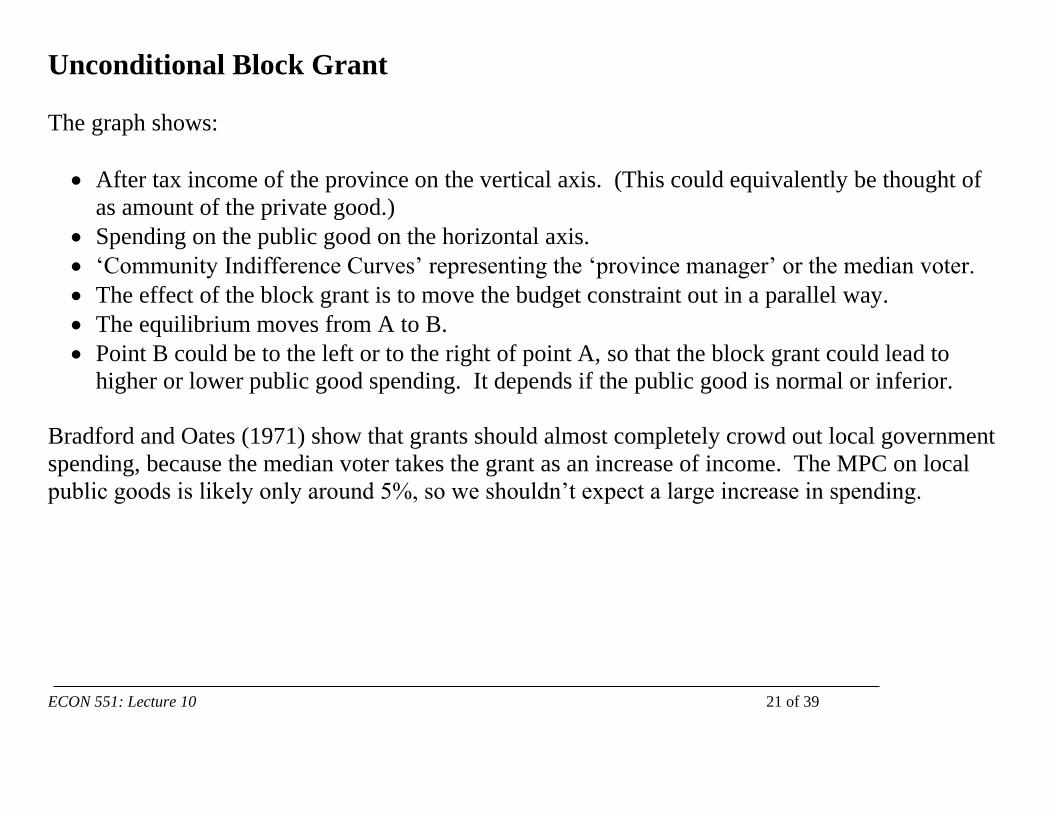
Conditional Block Grant

Imagine that the federal government now decides that they don’t like the spending decisions of the

subnational government and wants to influence their decisions.

Why might the feds choose a different level of spending than the subnational government?

• Different political preferences. Not the best reason – why impose the political preference of

the federal voters on the voters of one province.

• Externalities. This is a better reason. If providing a program had externalities, then the feds

might be able to better account for them than could any individual provinces. For example,

provinces might provide too small welfare programs because they are worried about mobility.

Migrants would come to take advantage of their benefits, so the provinces’ equilibrium

welfare rates are too low.


What does a conditional block grant look like?

• Initial equilibrium at C.

• Conditional grant means that you essentially

are given an extra endowment of the Public

Good, moving the budget constraint out

horizontally.

• If the local government just spent the new

money on the desired good, then E.

• HOWEVER, the local government re-

optimizes and ends up at D – part of the new

endowment gets consumed as tax cuts.

After

tax

income

Public

Good

U0

U1

D

C

E


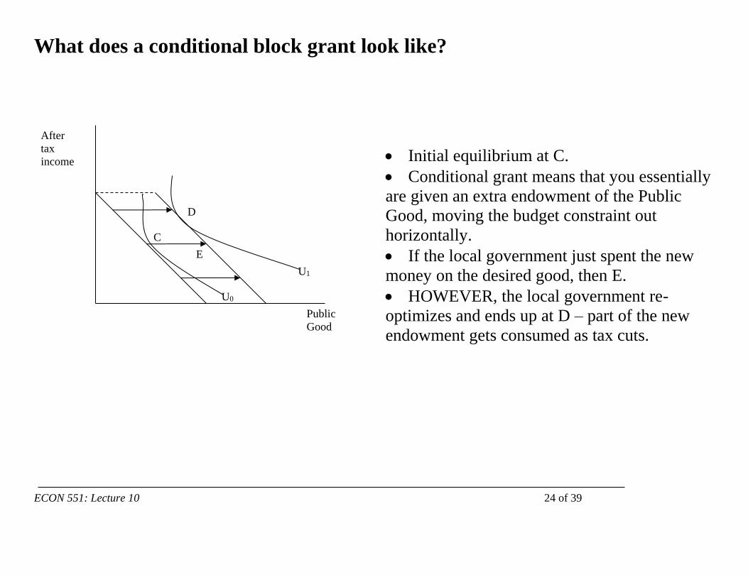
Matching Grant

So, imagine the feds care about the level of public goods spending at the provincial level. We have

seen that block grants might not lead to the desired level of public goods spending. Is there another

way?

What if the federal government offers a ‘matching grant’? This kind of grant offers a match for

every dollar spent at the subnational level.

For example, from 1966 to 1996, the Canada Assistance Plan was a federal transfer that paid $1 for

every dollar spent by provinces on social assistance (welfare) programs. Essentially, the provinces

were spending 50 cent dollars. Here’s what it looks like:


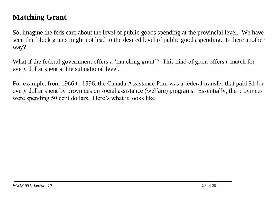
Matching Grant

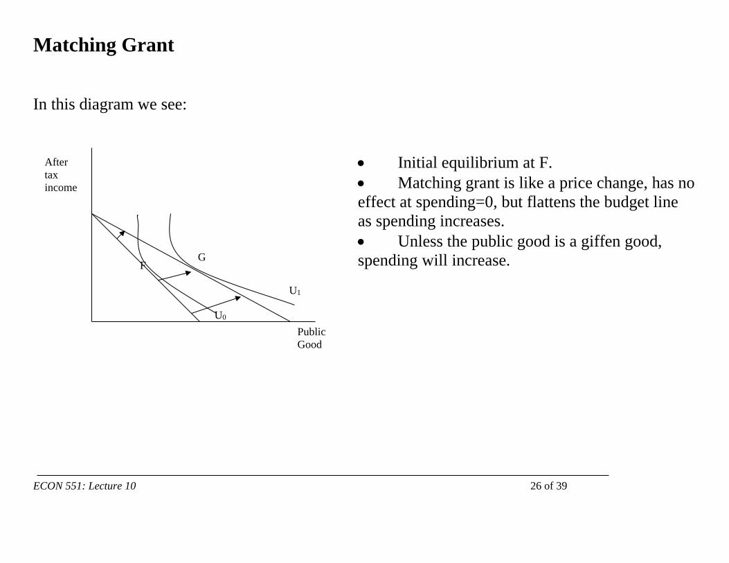
In this diagram we see:

• Initial equilibrium at F.

• Matching grant is like a price change, has no

effect at spending=0, but flattens the budget line

as spending increases.

• Unless the public good is a giffen good,

spending will increase.

After

tax

income

Public

Good

U0

U1

G F


What can go wrong here?

• If the feds want to get the right level of the PG, they have to choose the right match rate. This

might be hard.

• The feds don’t have any cost control—they just write cheques for however much the provinces

want to spend.

• Both of these factors came into play in the 1990s, with the cap on CAP, and then its cessation

with the start of the CHST.


Agenda

1. Overview





Equalization grants

Equalization grants are common in many countries across the world. Australia, Belgium, Spain,

Germany, Canada, South Africa, Japan.

• The United States is a bit unique in not having a large, dedicated, equalization scheme.

What is the goal of equalization grants?

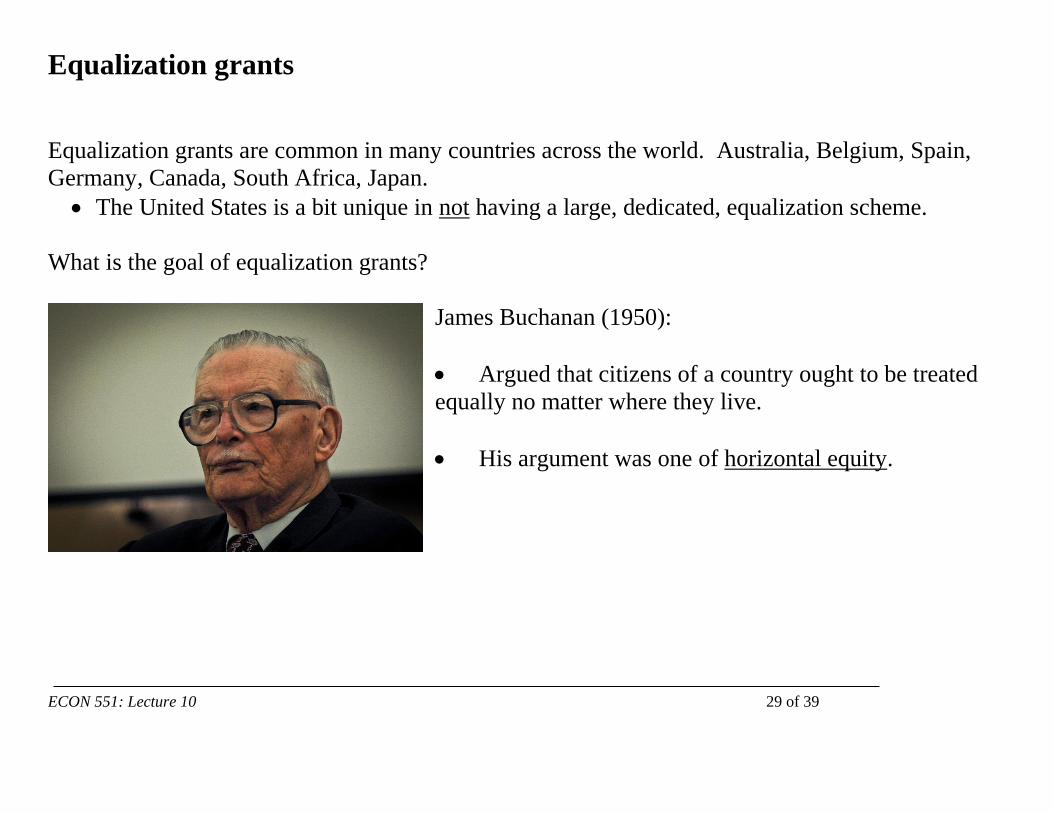
James Buchanan (1950):

• Argued that citizens of a country ought to be treated

equally no matter where they live.

• His argument was one of horizontal equity.


Why would a federal system lead to violations of horizontal equity?

• Imagine a country with subnational jurisdictions constitutionally mandated to provide certain

services.

• Say there is some resource that could be taxed locally or federally.

• If local taxation, then there will be incentive to move to get access to that government

spending.

• If central taxation, no incentive to move.

• Therefore, residency influenced by constitution in absence of equalization, not neutral.

Boadway (2004) notes substantial value judgement:

• For this model, we have to think the resource is not ‘owned’ by the province.


What about rich and poor?

Also note that we have not at all mentioned vertical equity.

• The goal of equalization grants is not about ‘poor’ and ‘rich’ people and trying to tax

according to the ability to pay.

• Neither is it about ‘poor’ and ‘rich’ regions necessarily—we care about people, not regions.

• Instead, equalization helps to forestall excessively high rates of taxation in resource poor

regions.

• In essence, this means saving the immobile rich in poor regions from having to pay high taxes

to fund a given level of services.


The Net Fiscal Benefit and Efficient Migration

Buchanan (1950) described a calculation that took the value of public services received and

subtracted the taxes paid.

• He referred to this difference as the fiscal residuum.

• This is now referred to as the net fiscal benefit or NFB.

NFB = value of public services – tax burden

The goal of equalization grants, is to eliminate differences in NFBs across jurisdictions.

• And thus, ensure fiscal neutrality for residency decisions.


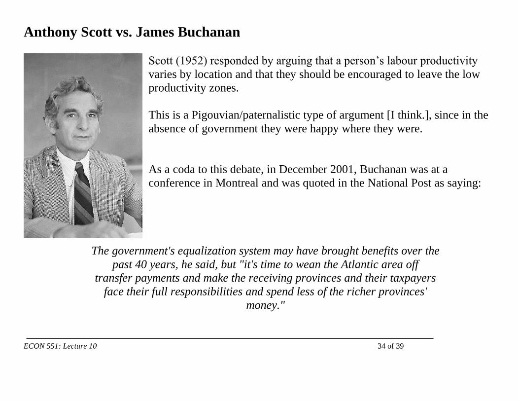
Anthony Scott vs. James Buchanan

Anthony Scott (1950) argued that equalization grants induce inefficient migration because it

encourages people to stay in resource-poor areas. His argument is often heard so, let’s look at it:

This objection is that such transfers provide amenities to poor people in resource-poor states, a

situation which may be undesirable in the long-run for the following reason: The maximum

income for the whole country, and so the highest average personal income, are to be achieved

only by maximizing national production. This in turn can be achieved only when resources and

labour are combined in such a way that the marginal product of similar units of labour is the

same in all places.

Buchanan (1952) rebuts this argument by arguing:

For resource effects in the geographical sense to be present; ie for an income transfer to be

resource distorting, like units of resource must be treated differently in different geographical

areas as a result of the transfer. Therefore, the argument applies only to transfers among regions

which involve differential fiscal treatment among individual ‘equals’ or among ‘like resource

units’.


Anthony Scott vs. James Buchanan

Scott (1952) responded by arguing that a person’s labour productivity

varies by location and that they should be encouraged to leave the low

productivity zones.

This is a Pigouvian/paternalistic type of argument [I think.], since in the

absence of government they were happy where they were.

As a coda to this debate, in December 2001, Buchanan was at a

conference in Montreal and was quoted in the National Post as saying:

The government's equalization system may have brought benefits over the

past 40 years, he said, but "it's time to wean the Atlantic area off

transfer payments and make the receiving provinces and their taxpayers

face their full responsibilities and spend less of the richer provinces'

money."


Canada’s Equalization Grant

The Constitution Act of 1982 mandates the federal government to provide some form of

equalization in Section 36, Part (2):

Parliament and the government of Canada are committed to the principle of making equalization

payments to ensure that provincial governments have sufficient revenues to provide reasonably

comparable levels of public services at reasonably comparable levels of taxation.

The formula has the following features:

• It takes 5 separate tax bases at the provincial level: PIT, CIT, Consumption, 50% resource

revenues and property+misc.

• 10 prov standard. From 1982-2004 it was 5-province. (BC, SK, MB, ON, QC)

• If the formula delivers a positive number—you get a cheque. If negative, you get nothing. For

this reason, it is called a ‘gross’ system, rather than ‘net’.

• NL and NS negotiated offsets for its resource revenues.

• 2009 a total spending cap was put on the program.


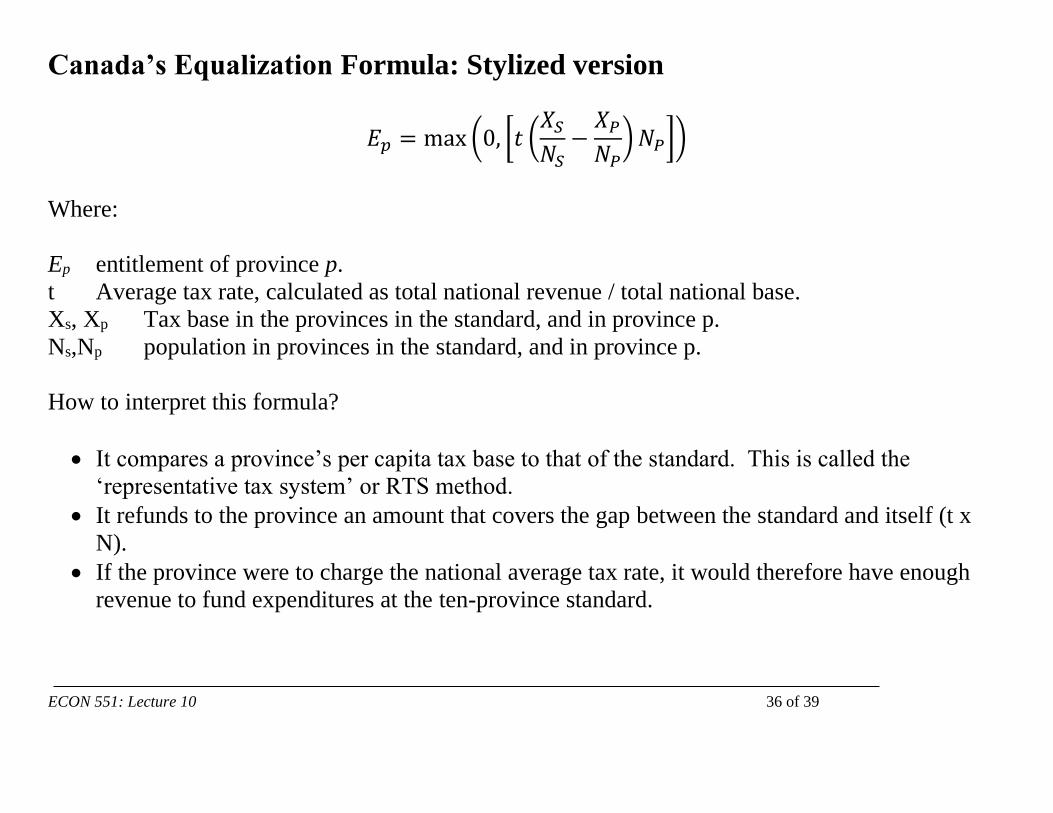
Canada’s Equalization Formula: Stylized version

𝐸𝑝 = max (0, [𝑡 (𝑋𝑆𝑁𝑆

−𝑋𝑃𝑁𝑃

)𝑁𝑃])

Where:

Ep entitlement of province p.

t Average tax rate, calculated as total national revenue / total national base.

Xs, Xp Tax base in the provinces in the standard, and in province p.

Ns,Np population in provinces in the standard, and in province p.

How to interpret this formula?

• It compares a province’s per capita tax base to that of the standard. This is called the

‘representative tax system’ or RTS method.

• It refunds to the province an amount that covers the gap between the standard and itself (t x

N).

• If the province were to charge the national average tax rate, it would therefore have enough

revenue to fund expenditures at the ten-province standard.


Some comments about the formula:

• Why did we ever use just five provinces? In 1982 this change was made. From most

accounts, it was simply a cost-saving measure. Including Alberta in the calculation would

increase the averages so much that the federal government would have to pay out a lot more.

o The end result is something far short of full equalization.

• Why use the tax base and not revenues? Because you don’t want the provincial government’s

choices to affect its allocation.

o Problem: Smart 1998 explores the effect of elastic tax bases—provinces might choose

‘too high’ tax rates in order to shrink the base and therefore get larger equalization

cheques.

o What incentive does this give provinces to increase their tax base—e.g. offshore

revenues in NL and NS.

• How to measure X? Different provinces have entirely different approaches to taxation. So,

some standard is needed, but is at times arbitrary and arcane. It doesn’t necessarily relate to

actual base definitions used in practice.


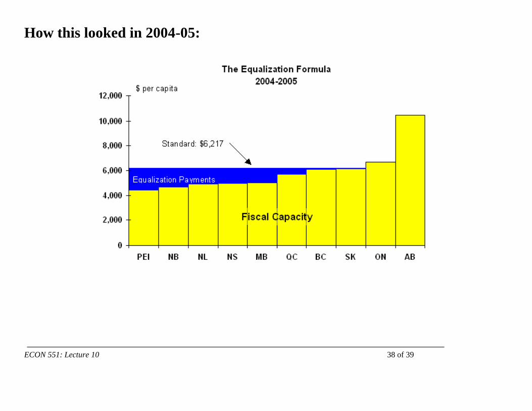
How this looked in 2004-05:

ECON551: Lecture 10 39

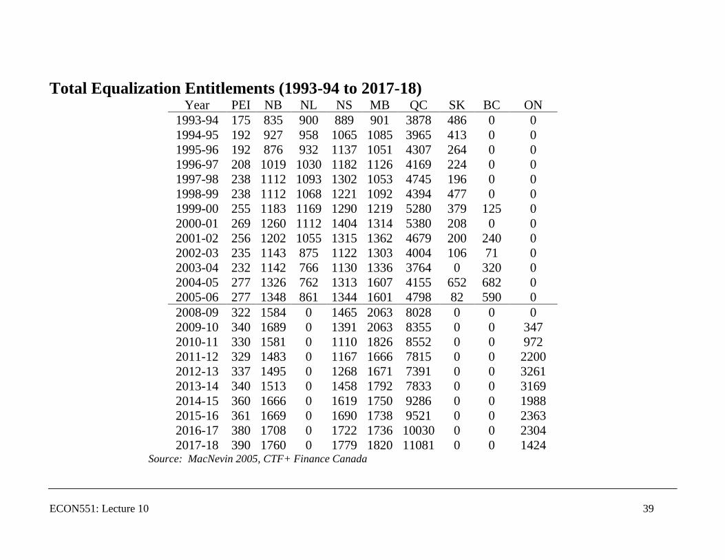
Total Equalization Entitlements (1993-94 to 2017-18) Year PEI NB NL NS MB QC SK BC ON

1993-94 175 835 900 889 901 3878 486 0 0

1994-95 192 927 958 1065 1085 3965 413 0 0

1995-96 192 876 932 1137 1051 4307 264 0 0

1996-97 208 1019 1030 1182 1126 4169 224 0 0

1997-98 238 1112 1093 1302 1053 4745 196 0 0

1998-99 238 1112 1068 1221 1092 4394 477 0 0

1999-00 255 1183 1169 1290 1219 5280 379 125 0

2000-01 269 1260 1112 1404 1314 5380 208 0 0

2001-02 256 1202 1055 1315 1362 4679 200 240 0

2002-03 235 1143 875 1122 1303 4004 106 71 0

2003-04 232 1142 766 1130 1336 3764 0 320 0

2004-05 277 1326 762 1313 1607 4155 652 682 0

2005-06 277 1348 861 1344 1601 4798 82 590 0

2008-09 322 1584 0 1465 2063 8028 0 0 0

2009-10 340 1689 0 1391 2063 8355 0 0 347

2010-11 330 1581 0 1110 1826 8552 0 0 972

2011-12 329 1483 0 1167 1666 7815 0 0 2200

2012-13 337 1495 0 1268 1671 7391 0 0 3261

2013-14 340 1513 0 1458 1792 7833 0 0 3169

2014-15 360 1666 0 1619 1750 9286 0 0 1988

2015-16 361 1669 0 1690 1738 9521 0 0 2363

2016-17 380 1708 0 1722 1736 10030 0 0 2304

2017-18 390 1760 0 1779 1820 11081 0 0 1424 Source: MacNevin 2005, CTF+ Finance Canada

Documents

Econ 551 Government Finance: Revenues Winter 2018faculty.arts.ubc.ca/kmilligan/teaching/ECON551/551-slides-10.pdf · Government Finance: Revenues ... Oates and ‘fiscal federalism