Embed Size (px)
Citation preview
Econ 492: Comparative Financial Crises
Lecture 114 September 2011
David LongworthThis material is copyrighted and is for the sole use of students registered in ECON 492. This material
shall not be distributed or disseminated to anyone other than students registered on ECON 492. Failure to abide by these conditions is a breach of copyright, and may also constitute a breach of academic
integrity under the University Senate’s Academic Integrity Policy Statement.
Economics 492 Lecture 1 2
Overview
I. IntroductionII. Financial System: Overview III. Causes of Financial CrisesIV. Prediction of Financial Crises
Note: AG indicates Franklin Allen and Douglas Gale (2009), Understanding Financial Crises. KA indicates Charles P. Kindleberger and Robert Aliber (2005), Manias, Panics, and Crashes.

Economics 492 Lecture 1 3
l. Introduction
• Introductions

Economics 492 Lecture 1 4
l. Introduction
• Introductions• August 2007
Economics 492 Lecture 1 5
l. Introduction
• Introductions• August 2007• Outline of Course (handout)
Economics 492 Lecture 1 6
l. Introduction
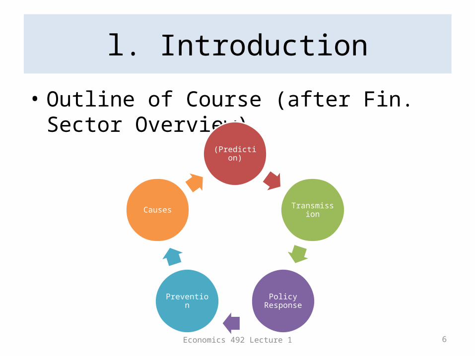
• Outline of Course (after Fin. Sector Overview)
(Prediction)
Transmission
Policy ResponsePrevention
Causes

Economics 492 Lecture 1 7
l. Introduction
• The paper• Presentation and discussion• Participation• Schedule– Lecture next week– 28 September: your (one paragraph) topic due– 5 October: your 2-page outline due– 5 – 26 October (and beyond): weekly consultations– 2 or 9– 23 November: presentations– 30 November: paper due in class and class discussion
Economics 492 Lecture 1 8
II. Financial System: Overview
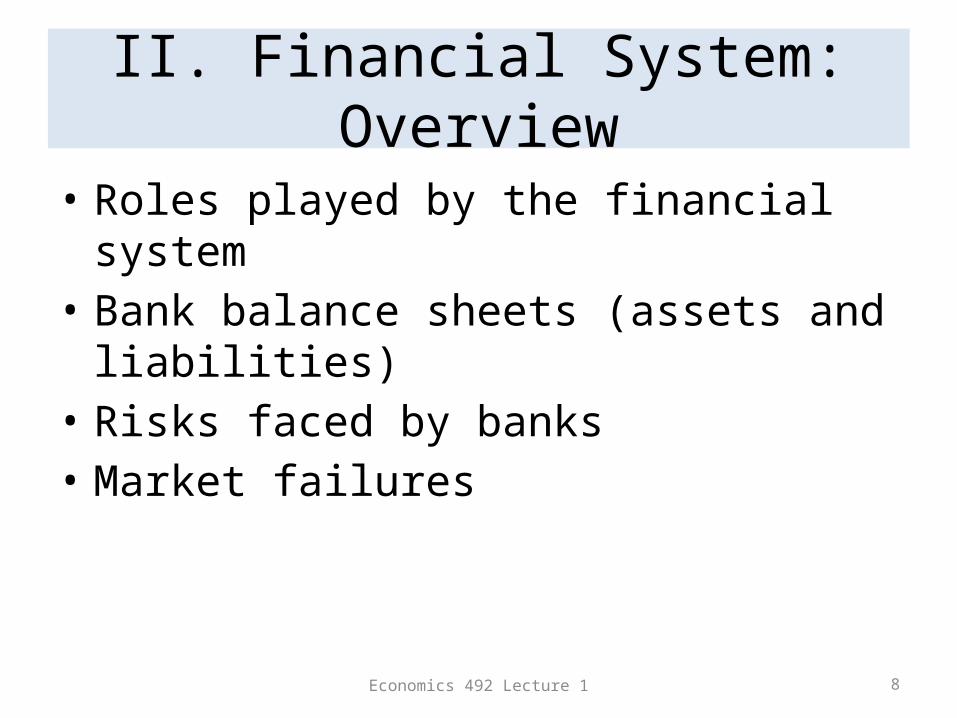
• Roles played by the financial system• Bank balance sheets (assets and liabilities)• Risks faced by banks• Market failures
Economics 492 Lecture 1 9
II. Financial System: Overview
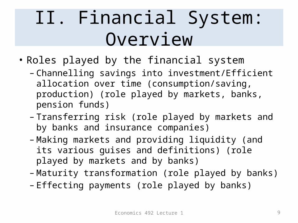
• Roles played by the financial system– Channelling savings into investment/Efficient allocation
over time (consumption/saving, production) (role played by markets, banks, pension funds)
– Transferring risk (role played by markets and by banks and insurance companies)
– Making markets and providing liquidity (and its various guises and definitions) (role played by markets and by banks)
– Maturity transformation (role played by banks)– Effecting payments (role played by banks)
Economics 492 Lecture 1 10
II. Financial System: Overview
• Roles played by the financial system– Channelling savings into investment/Efficient
allocation over time (consumption/saving, production) (role played by markets and by banks)
Economics 492 Lecture 1 11
II. Financial System: Overview
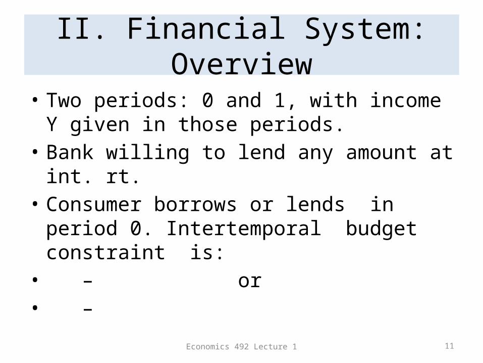
• Two periods: 0 and 1, with income Y given in those periods.
• Bank willing to lend any amount at int. rt. • Consumer borrows or lends in period 0. Intertemporal budget constraint is:• – or• –
Economics 492 Lecture 1 12
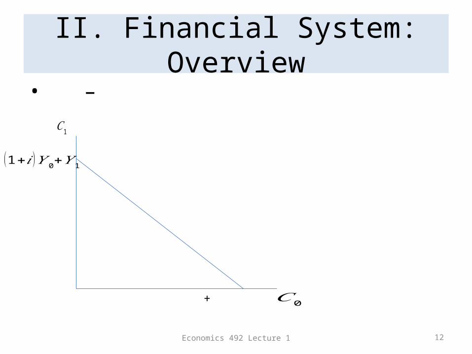
II. Financial System: Overview• –
𝐶0+
𝐶1
(1+𝑖 )𝑌 0+𝑌 1
Economics 492 Lecture 1 13
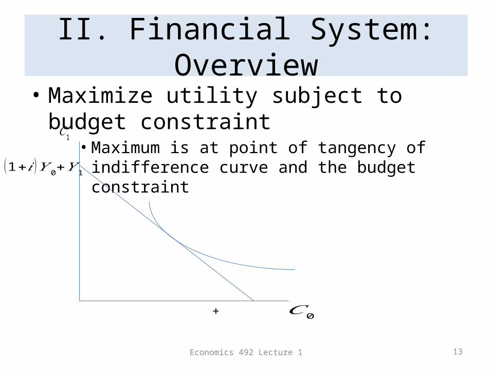
II. Financial System: Overview• Maximize utility subject to budget constraint
• Maximum is at point of tangency of indifference curve and the budget constraint
𝐶0+
𝐶1
(1+𝑖 )𝑌 0+𝑌 1
Economics 492 Lecture 1 14
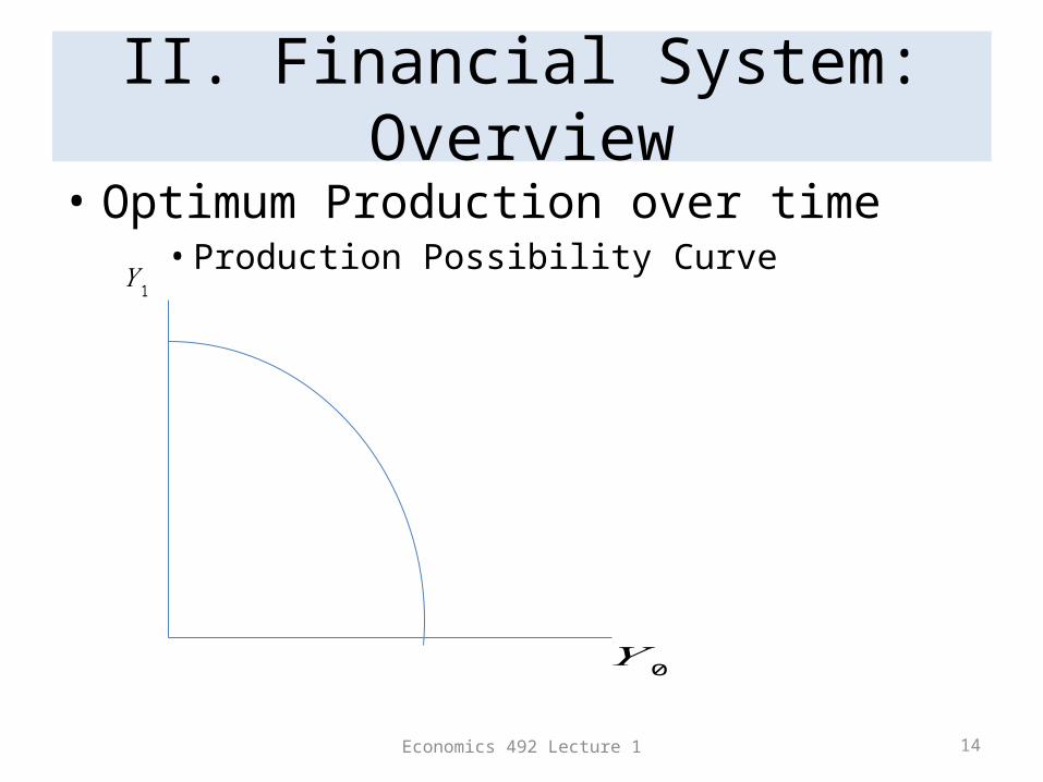
II. Financial System: Overview• Optimum Production over time
• Production Possibility Curve
𝑌 0
𝑌 1
Economics 492 Lecture 1 15
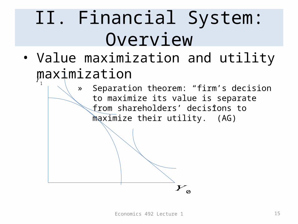
II. Financial System: Overview• Value maximization and utility maximization
» Separation theorem: “firm’s decision to maximize its value is separate from shareholders’ decisions to maximize their utility.” (AG)
𝑌 0
𝑌 1
Economics 492 Lecture 1 16
II. Financial System: Overview
• Roles played by the financial system– Transferring Risk (role played by markets and by banks
and insurance companies)• Risk sharing
– There is always uncertainty about the future, e.g. income– Contingent commodity: “a good whose delivery is contingent on the
occurrence of a particular state of nature” (AG)– Two equivalent ways to achieving an efficient allocation of risk
» If there are complete markets for contingent commodities, i.e. there are markets for each contingent commodity, and consumers only have to satisfy their budget constraint
» If there are Arrow securities for each state, securities which are a “promise to deliver one unit of money if a given state occurs and nothing otherwise.” (AG)
Economics 492 Lecture 1 17
II. Financial System: Overview
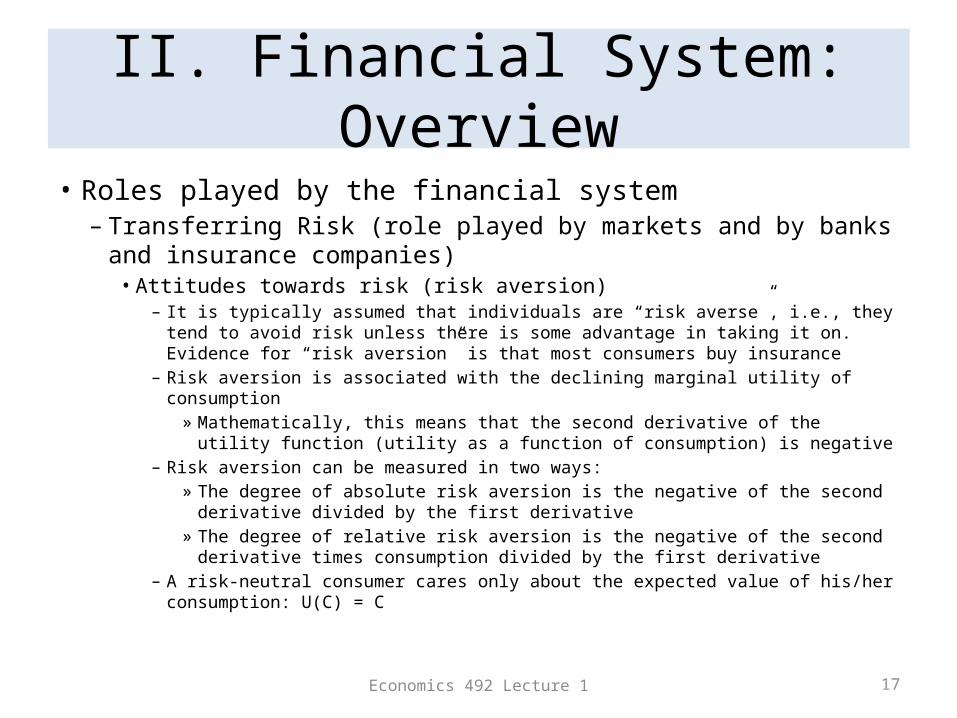
• Roles played by the financial system– Transferring Risk (role played by markets and by banks and insurance
companies)• Attitudes towards risk (risk aversion)
– It is typically assumed that individuals are “risk averse”, i.e., they tend to avoid risk unless there is some advantage in taking it on. Evidence for “risk aversion” is that most consumers buy insurance
– Risk aversion is associated with the declining marginal utility of consumption » Mathematically, this means that the second derivative of the utility function
(utility as a function of consumption) is negative– Risk aversion can be measured in two ways:
» The degree of absolute risk aversion is the negative of the second derivative divided by the first derivative
» The degree of relative risk aversion is the negative of the second derivative times consumption divided by the first derivative
– A risk-neutral consumer cares only about the expected value of his/her consumption: U(C) = C
Economics 492 Lecture 1 18
II. Financial System: Overview
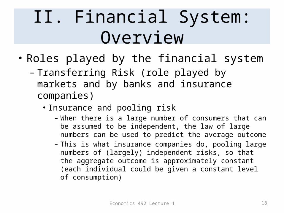
• Roles played by the financial system– Transferring Risk (role played by markets and by
banks and insurance companies)• Insurance and pooling risk
– When there is a large number of consumers that can be assumed to be independent, the law of large numbers can be used to predict the average outcome
– This is what insurance companies do, pooling large numbers of (largely) independent risks, so that the aggregate outcome is approximately constant (each individual could be given a constant level of consumption)
Economics 492 Lecture 1 19
II. Financial System: Overview
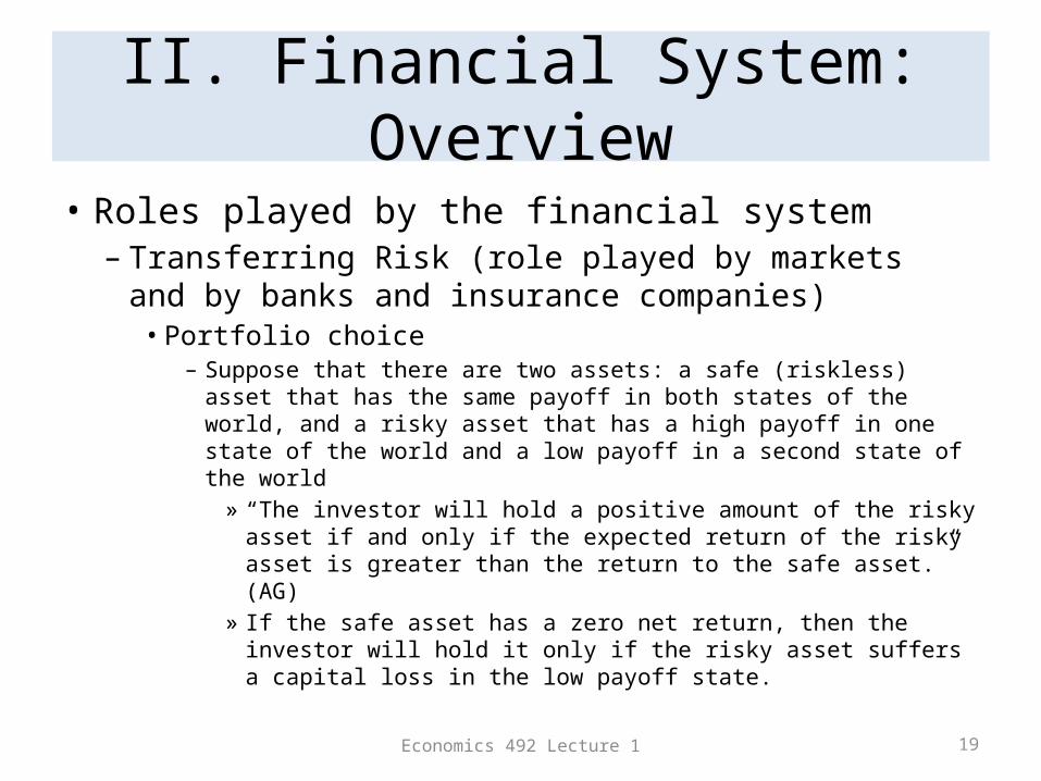
• Roles played by the financial system– Transferring Risk (role played by markets and by banks
and insurance companies)• Portfolio choice
– Suppose that there are two assets: a safe (riskless) asset that has the same payoff in both states of the world, and a risky asset that has a high payoff in one state of the world and a low payoff in a second state of the world» “The investor will hold a positive amount of the risky asset if
and only if the expected return of the risky asset is greater than the return to the safe asset.” (AG)
» If the safe asset has a zero net return, then the investor will hold it only if the risky asset suffers a capital loss in the low payoff state.
Economics 492 Lecture 1 20
II. Financial System: Overview
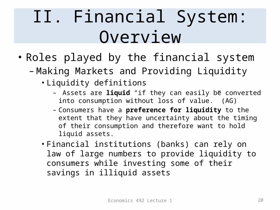
• Roles played by the financial system– Making Markets and Providing Liquidity• Liquidity definitions
– Assets are liquid “if they can easily be converted into consumption without loss of value.” (AG)
– Consumers have a preference for liquidity to the extent that they have uncertainty about the timing of their consumption and therefore want to hold liquid assets.
• Financial institutions (banks) can rely on law of large numbers to provide liquidity to consumers while investing some of their savings in illiquid assets
Economics 492 Lecture 1 21
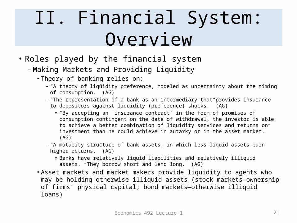
II. Financial System: Overview• Roles played by the financial system
– Making Markets and Providing Liquidity• Theory of banking relies on:
– “A theory of liquidity preference, modeled as uncertainty about the timing of consumption.” (AG)
– “The representation of a bank as an intermediary that provides insurance to depositors against liquidity (preference) shocks.” (AG)» “By accepting an ‘insurance contract’ in the form of promises of consumption
contingent on the date of withdrawal, the investor is able to achieve a better combination of liquidity services and returns on investment than he could achieve in autarky or in the asset market.” (AG)
– “A maturity structure of bank assets, in which less liquid assets earn higher returns.” (AG)» Banks have relatively liquid liabilities and relatively illiquid assets. “They borrow
short and lend long.” (AG)
• Asset markets and market makers provide liquidity to agents who may be holding otherwise illiquid assets (stock markets—ownership of firms’ physical capital; bond markets—otherwise illiquid loans)
Economics 492 Lecture 1 22
II. Financial System: Overview
• Roles played by the financial system– Maturity transformation (role played by banks)
• As we have already seen, banks tend to have shorter-term liabilities than the maturity of their assets
– Effecting Payments (role played by banks)• This is another reason why consumers place deposits
with banks. It is extremely difficult for consumers not to transact with banks because of this. Currency and demand deposits are close to perfect substitutes, but it is difficult to make large payments with currency.
Economics 492 Lecture 1 23
II. Financial System: Overview
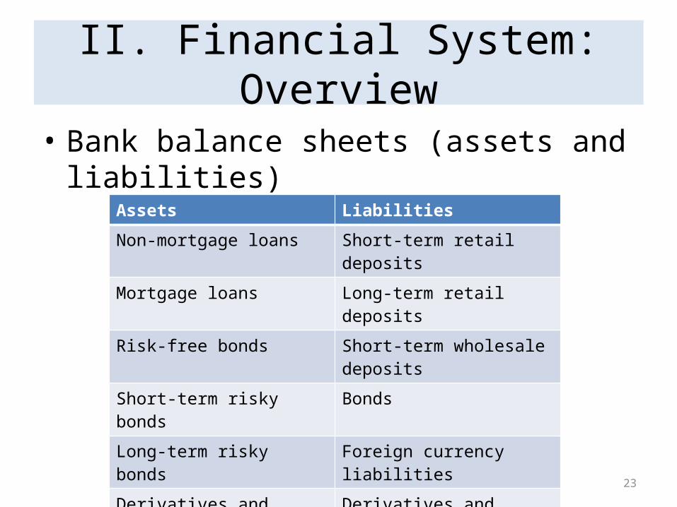
• Bank balance sheets (assets and liabilities)
Assets Liabilities
Non-mortgage loans Short-term retail deposits
Mortgage loans Long-term retail deposits
Risk-free bonds Short-term wholesale deposits
Short-term risky bonds Bonds
Long-term risky bonds Foreign currency liabilities
Derivatives and repos Derivatives and repos
Foreign currency assets Equity (capital)
Total Assets equals Total Liabilities
Economics 492 Lecture 1 24
II. Financial System: Overview
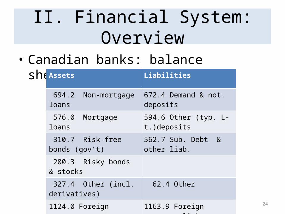
• Canadian banks: balance sheet(May ‘11, $bn.)Assets Liabilities
694.2 Non-mortgage loans 672.4 Demand & not. deposits
576.0 Mortgage loans 594.6 Other (typ. L-t.)deposits
310.7 Risk-free bonds (gov’t) 562.7 Sub. Debt & other liab.
200.3 Risky bonds & stocks
327.4 Other (incl. derivatives) 62.4 Other
1124.0 Foreign currency assets 1163.9 Foreign currency liab.
176.6 Shareholder equity
3232.6 Total Assets equals 3232.6 Total Liabilities
Economics 492 Lecture 1 25
II. Financial System: Overview
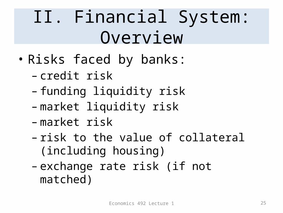
• Risks faced by banks: – credit risk– funding liquidity risk– market liquidity risk– market risk– risk to the value of collateral (including housing) – exchange rate risk (if not matched)
Economics 492 Lecture 1 26
II. Financial System: Overview
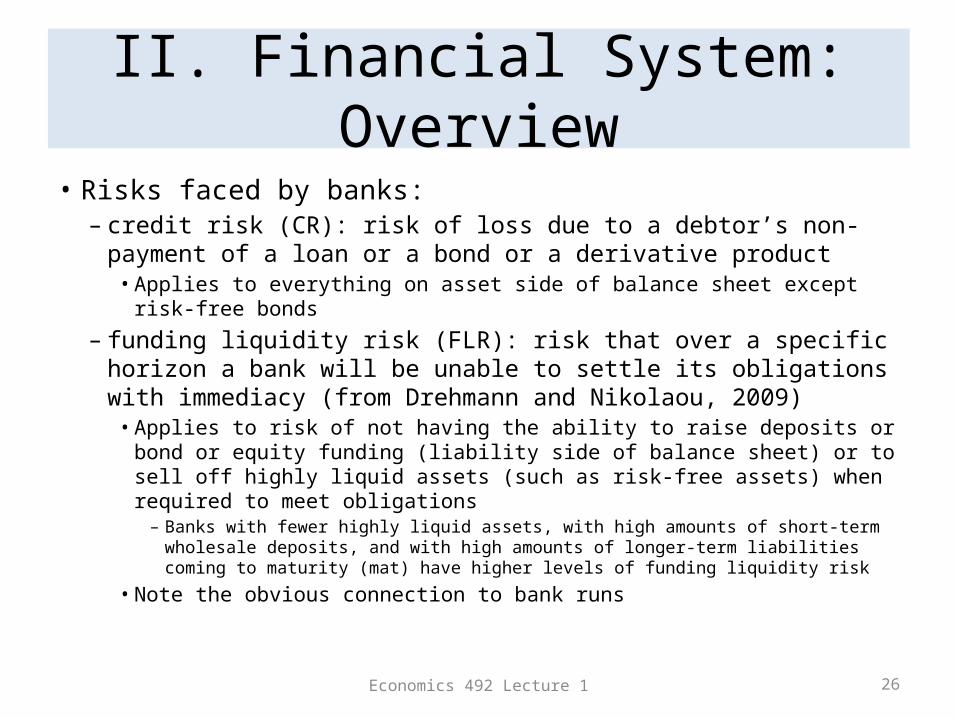
• Risks faced by banks: – credit risk (CR): risk of loss due to a debtor’s non-payment of a loan
or a bond or a derivative product• Applies to everything on asset side of balance sheet except risk-free bonds
– funding liquidity risk (FLR): risk that over a specific horizon a bank will be unable to settle its obligations with immediacy (from Drehmann and Nikolaou, 2009)• Applies to risk of not having the ability to raise deposits or bond or equity
funding (liability side of balance sheet) or to sell off highly liquid assets (such as risk-free assets) when required to meet obligations– Banks with fewer highly liquid assets, with high amounts of short-term wholesale
deposits, and with high amounts of longer-term liabilities coming to maturity (mat) have higher levels of funding liquidity risk
• Note the obvious connection to bank runs
Economics 492 Lecture 1 27
II. Financial System: Overview
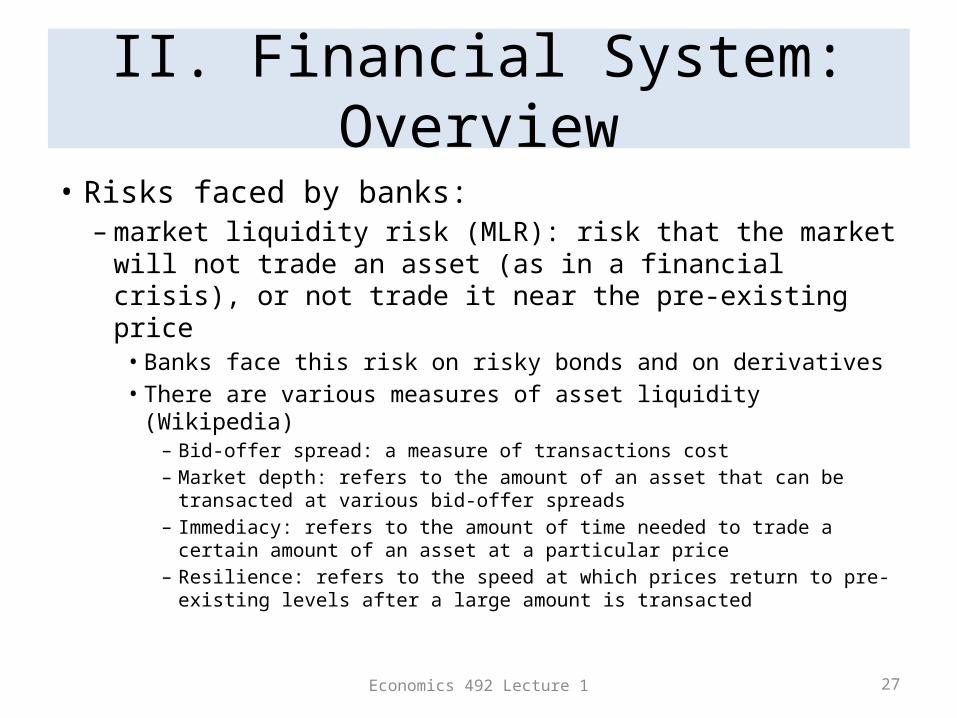
• Risks faced by banks: – market liquidity risk (MLR): risk that the market will not
trade an asset (as in a financial crisis), or not trade it near the pre-existing price• Banks face this risk on risky bonds and on derivatives• There are various measures of asset liquidity (Wikipedia)
– Bid-offer spread: a measure of transactions cost– Market depth: refers to the amount of an asset that can be
transacted at various bid-offer spreads– Immediacy: refers to the amount of time needed to trade a certain
amount of an asset at a particular price– Resilience: refers to the speed at which prices return to pre-existing
levels after a large amount is transacted
Economics 492 Lecture 1 28
II. Financial System: Overview
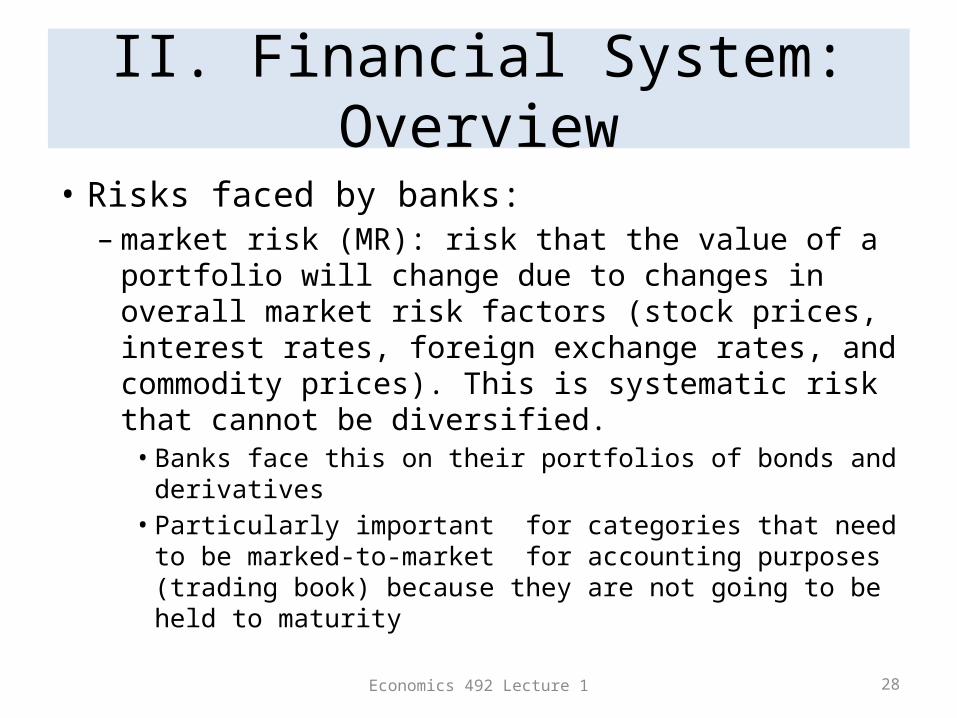
• Risks faced by banks: – market risk (MR): risk that the value of a portfolio
will change due to changes in overall market risk factors (stock prices, interest rates, foreign exchange rates, and commodity prices). This is systematic risk that cannot be diversified.• Banks face this on their portfolios of bonds and
derivatives• Particularly important for categories that need to be
marked-to-market for accounting purposes (trading book) because they are not going to be held to maturity
Economics 492 Lecture 1 29
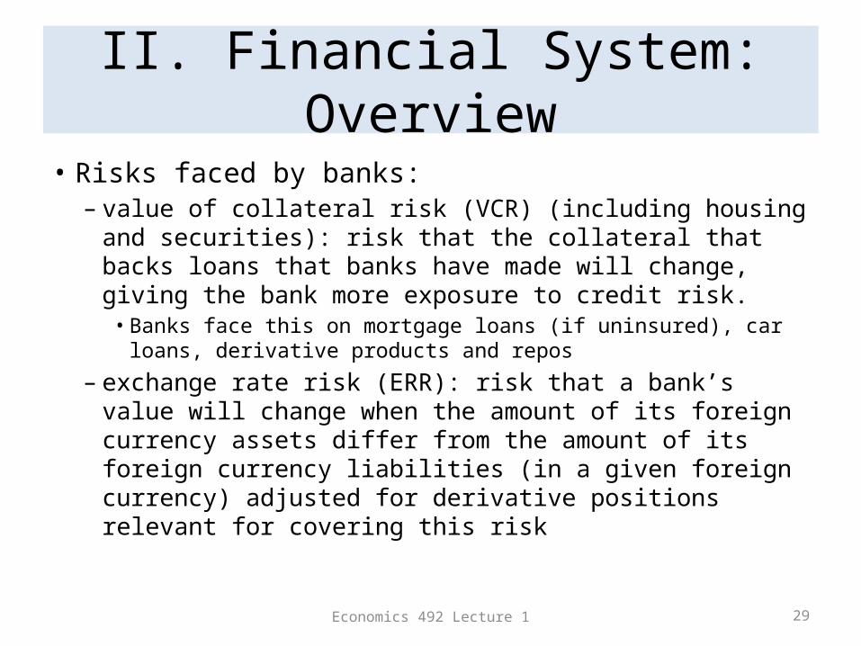
II. Financial System: Overview
• Risks faced by banks: – value of collateral risk (VCR) (including housing and
securities): risk that the collateral that backs loans that banks have made will change, giving the bank more exposure to credit risk.• Banks face this on mortgage loans (if uninsured), car loans,
derivative products and repos
– exchange rate risk (ERR): risk that a bank’s value will change when the amount of its foreign currency assets differ from the amount of its foreign currency liabilities (in a given foreign currency) adjusted for derivative positions relevant for covering this risk
Economics 492 Lecture 1 30
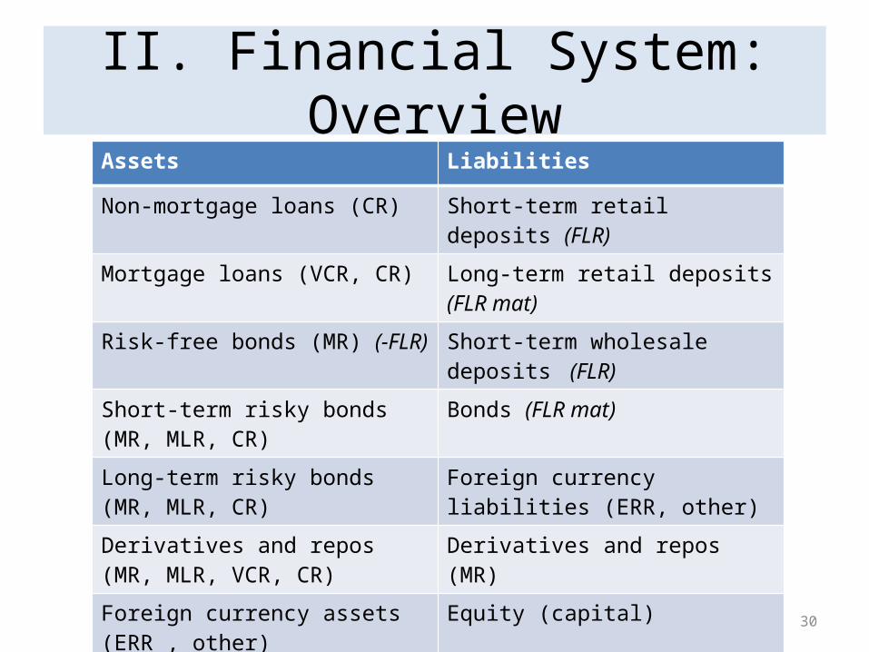
II. Financial System: OverviewAssets Liabilities
Non-mortgage loans (CR) Short-term retail deposits (FLR)
Mortgage loans (VCR, CR) Long-term retail deposits (FLR mat)
Risk-free bonds (MR) (-FLR) Short-term wholesale deposits (FLR)
Short-term risky bonds (MR, MLR, CR)
Bonds (FLR mat)
Long-term risky bonds (MR, MLR, CR) Foreign currency liabilities (ERR, other)
Derivatives and repos (MR, MLR, VCR, CR)
Derivatives and repos (MR)
Foreign currency assets (ERR , other) Equity (capital)
Economics 492 Lecture 1 31
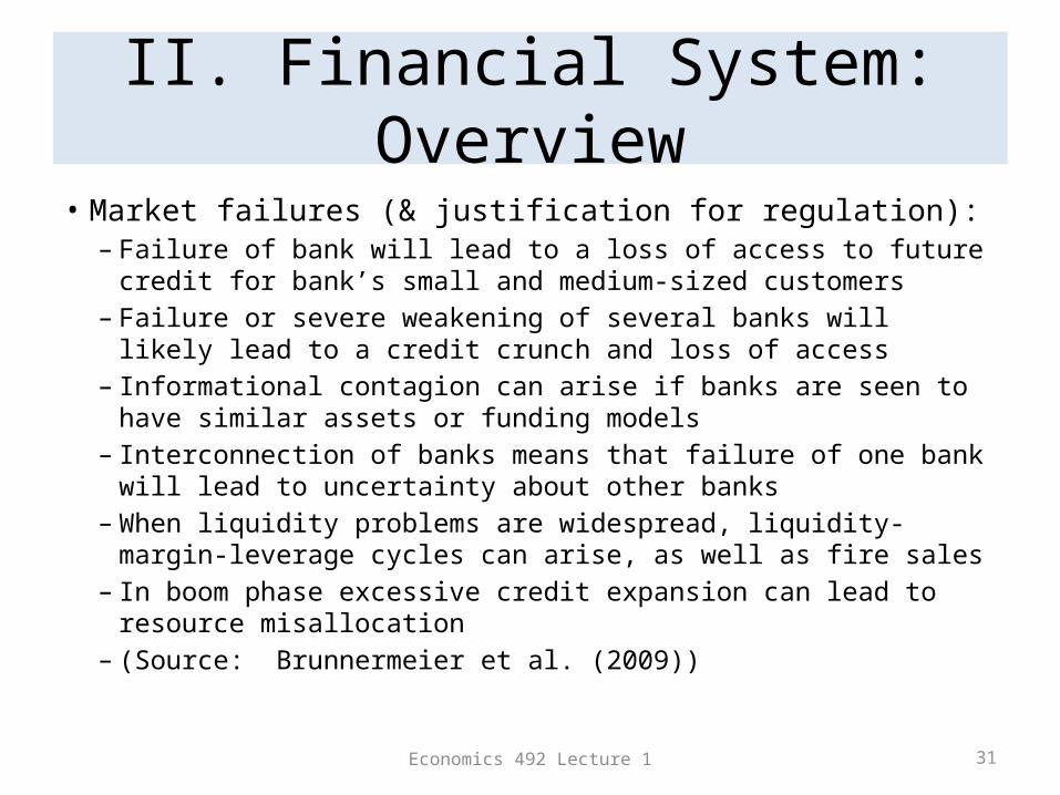
II. Financial System: Overview• Market failures (& justification for regulation):
– Failure of bank will lead to a loss of access to future credit for bank’s small and medium-sized customers
– Failure or severe weakening of several banks will likely lead to a credit crunch and loss of access
– Informational contagion can arise if banks are seen to have similar assets or funding models
– Interconnection of banks means that failure of one bank will lead to uncertainty about other banks
– When liquidity problems are widespread, liquidity-margin-leverage cycles can arise, as well as fire sales
– In boom phase excessive credit expansion can lead to resource misallocation
– (Source: Brunnermeier et al. (2009))
Economics 492 Lecture 1 32
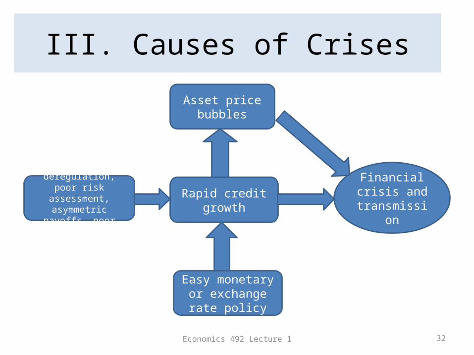
III. Causes of Crises
Innovation, deregulation, poor risk assessment,
asymmetric payoffs, poor government policy
Asset price bubbles
Rapid credit growth
Easy monetary or exchange rate
policy
Financial crisis and
transmission
Economics 492 Lecture 1 33
III. Causes of Crises
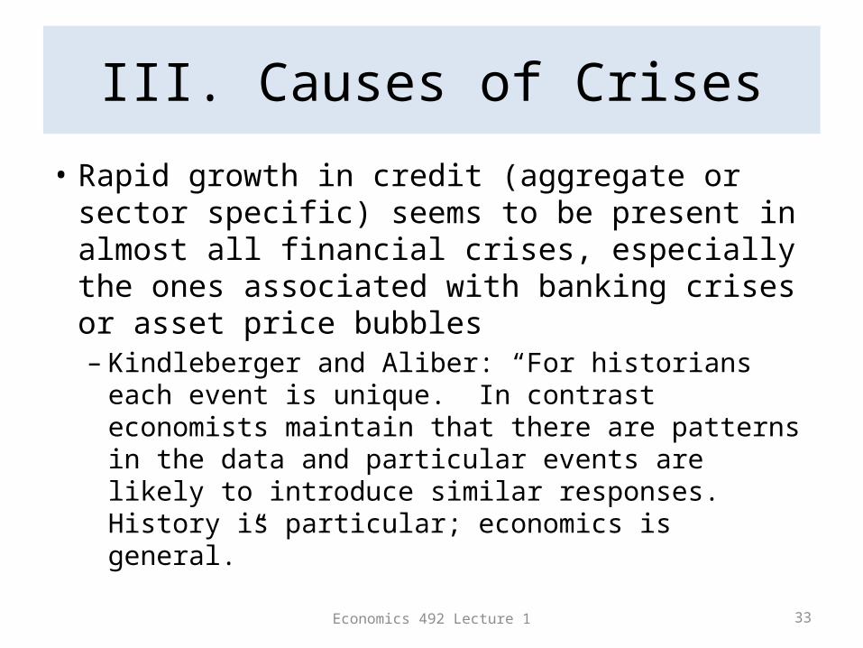
• Rapid growth in credit (aggregate or sector specific) seems to be present in almost all financial crises, especially the ones associated with banking crises or asset price bubbles – Kindleberger and Aliber: “For historians each
event is unique. In contrast economists maintain that there are patterns in the data and particular events are likely to introduce similar responses. History is particular; economics is general.”
Economics 492 Lecture 1 34
III. Causes of Crises
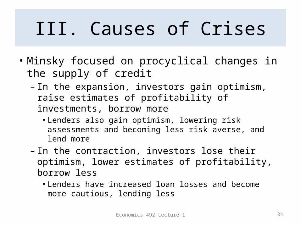
• Minsky focused on procyclical changes in the supply of credit– In the expansion, investors gain optimism, raise
estimates of profitability of investments, borrow more• Lenders also gain optimism, lowering risk assessments and
becoming less risk averse, and lend more
– In the contraction, investors lose their optimism, lower estimates of profitability, borrow less• Lenders have increased loan losses and become more
cautious, lending less
Economics 492 Lecture 1 35
III. Causes of Crises
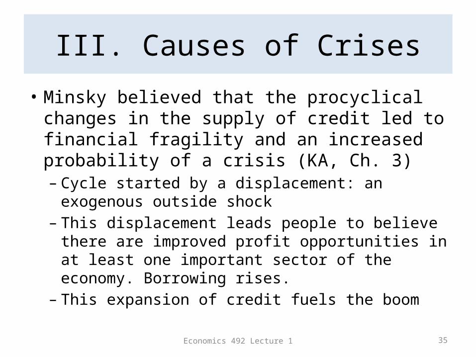
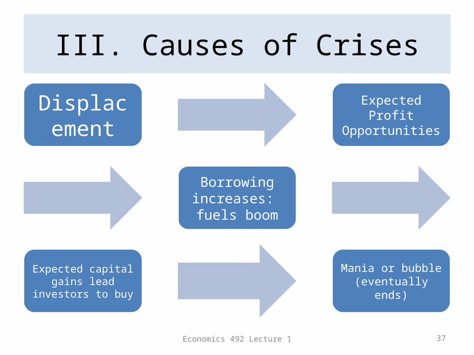
• Minsky believed that the procyclical changes in the supply of credit led to financial fragility and an increased probability of a crisis (KA, Ch. 3)– Cycle started by a displacement: an exogenous
outside shock– This displacement leads people to believe there are
improved profit opportunities in at least one important sector of the economy. Borrowing rises.
– This expansion of credit fuels the boom
Economics 492 Lecture 1 36
III. Causes of Crises
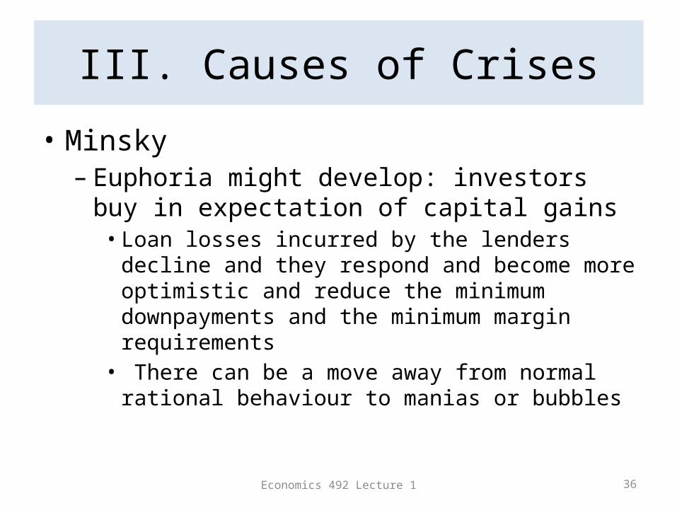
• Minsky– Euphoria might develop: investors buy in
expectation of capital gains• Loan losses incurred by the lenders decline and they
respond and become more optimistic and reduce the minimum downpayments and the minimum margin requirements• There can be a move away from normal rational
behaviour to manias or bubbles
Economics 492 Lecture 1 37
III. Causes of Crises
Displacement
Expected Profit Opportunities
Borrowing increases: fuels boom
Expected capital gains lead
investors to buy
Mania or bubble (eventually
ends)
Economics 492 Lecture 1 38
III. Causes of Crises
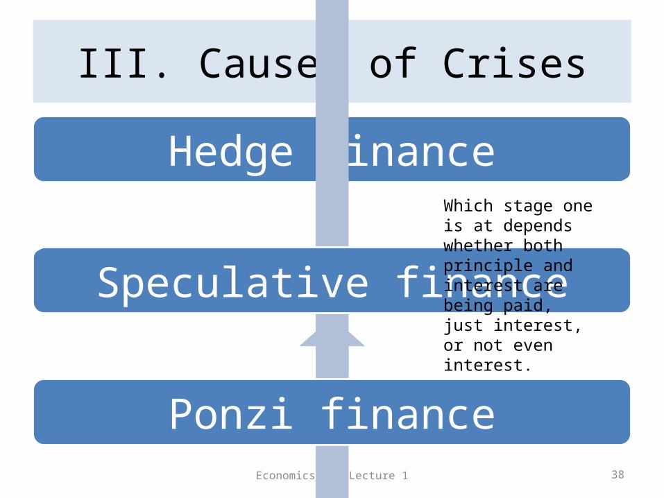
Hedge finance
Speculative finance
Ponzi finance
Which stage one is at depends whether both principle and interest are being paid, just interest, or not even interest.
Economics 492 Lecture 1 39
III. Causes of Crises
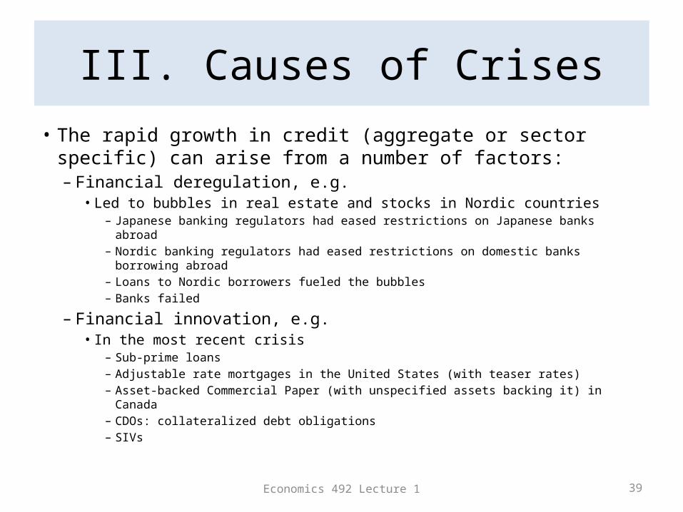
• The rapid growth in credit (aggregate or sector specific) can arise from a number of factors:– Financial deregulation, e.g.
• Led to bubbles in real estate and stocks in Nordic countries– Japanese banking regulators had eased restrictions on Japanese banks abroad– Nordic banking regulators had eased restrictions on domestic banks borrowing abroad– Loans to Nordic borrowers fueled the bubbles– Banks failed
– Financial innovation, e.g.• In the most recent crisis
– Sub-prime loans– Adjustable rate mortgages in the United States (with teaser rates)– Asset-backed Commercial Paper (with unspecified assets backing it) in Canada– CDOs: collateralized debt obligations– SIVs
Economics 492 Lecture 1 40
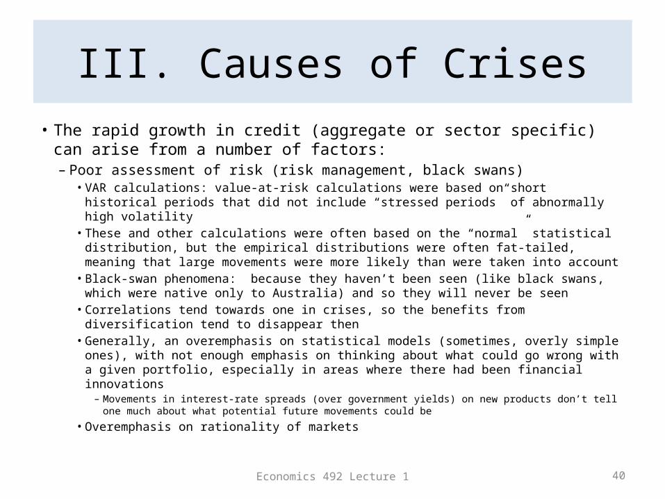
III. Causes of Crises• The rapid growth in credit (aggregate or sector specific) can arise from a
number of factors:– Poor assessment of risk (risk management, black swans)
• VAR calculations: value-at-risk calculations were based on short historical periods that did not include “stressed periods” of abnormally high volatility
• These and other calculations were often based on the “normal” statistical distribution, but the empirical distributions were often fat-tailed, meaning that large movements were more likely than were taken into account
• Black-swan phenomena: because they haven’t been seen (like black swans, which were native only to Australia) and so they will never be seen
• Correlations tend towards one in crises, so the benefits from diversification tend to disappear then
• Generally, an overemphasis on statistical models (sometimes, overly simple ones), with not enough emphasis on thinking about what could go wrong with a given portfolio, especially in areas where there had been financial innovations– Movements in interest-rate spreads (over government yields) on new products don’t tell one much
about what potential future movements could be
• Overemphasis on rationality of markets
Economics 492 Lecture 1 41
III. Causes of Crises
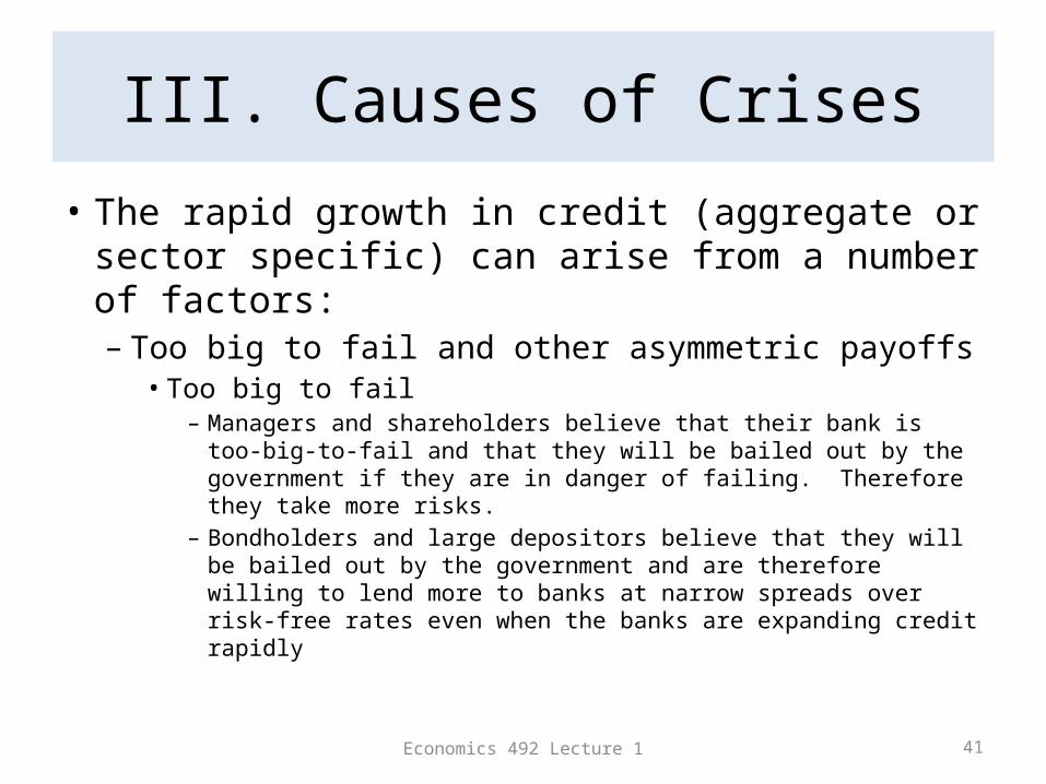
• The rapid growth in credit (aggregate or sector specific) can arise from a number of factors:– Too big to fail and other asymmetric payoffs• Too big to fail
– Managers and shareholders believe that their bank is too-big-to-fail and that they will be bailed out by the government if they are in danger of failing. Therefore they take more risks.
– Bondholders and large depositors believe that they will be bailed out by the government and are therefore willing to lend more to banks at narrow spreads over risk-free rates even when the banks are expanding credit rapidly
Economics 492 Lecture 1 42
III. Causes of Crises
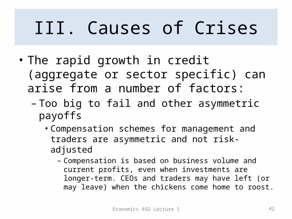
• The rapid growth in credit (aggregate or sector specific) can arise from a number of factors:– Too big to fail and other asymmetric payoffs• Compensation schemes for management and traders
are asymmetric and not risk-adjusted– Compensation is based on business volume and current
profits, even when investments are longer-term. CEOs and traders may have left (or may leave) when the chickens come home to roost.
Economics 492 Lecture 1 43
III. Causes of Crises
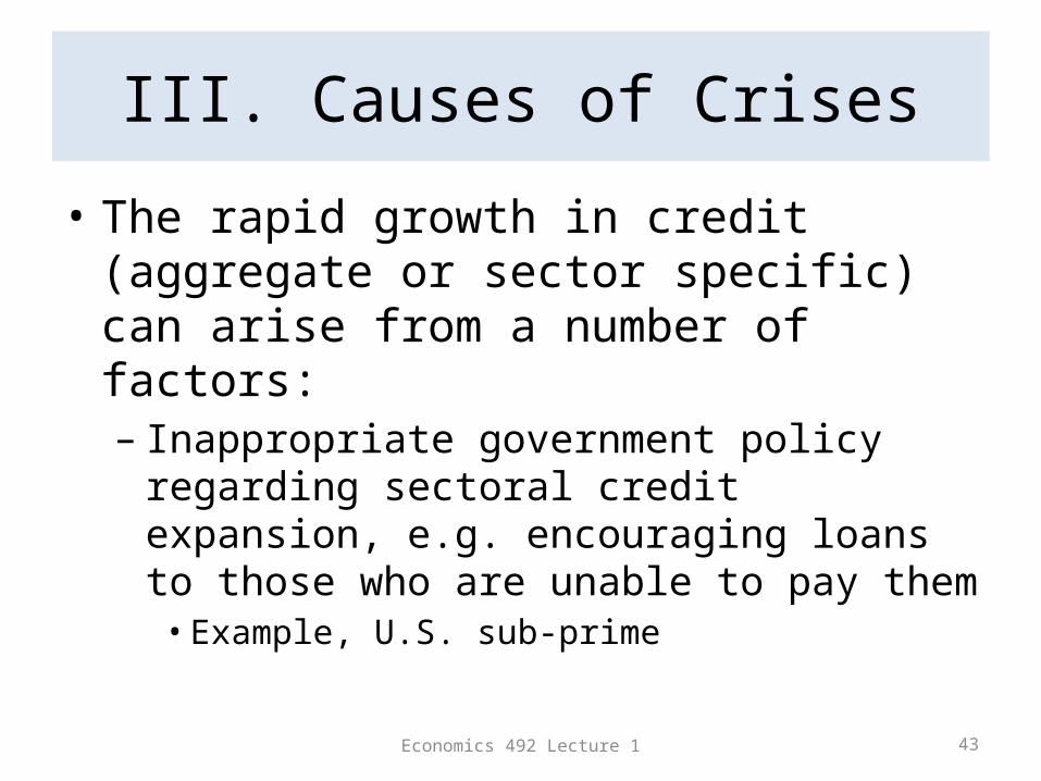
• The rapid growth in credit (aggregate or sector specific) can arise from a number of factors:– Inappropriate government policy regarding
sectoral credit expansion, e.g. encouraging loans to those who are unable to pay them• Example, U.S. sub-prime
Economics 492 Lecture 1 44
III. Causes of Crises
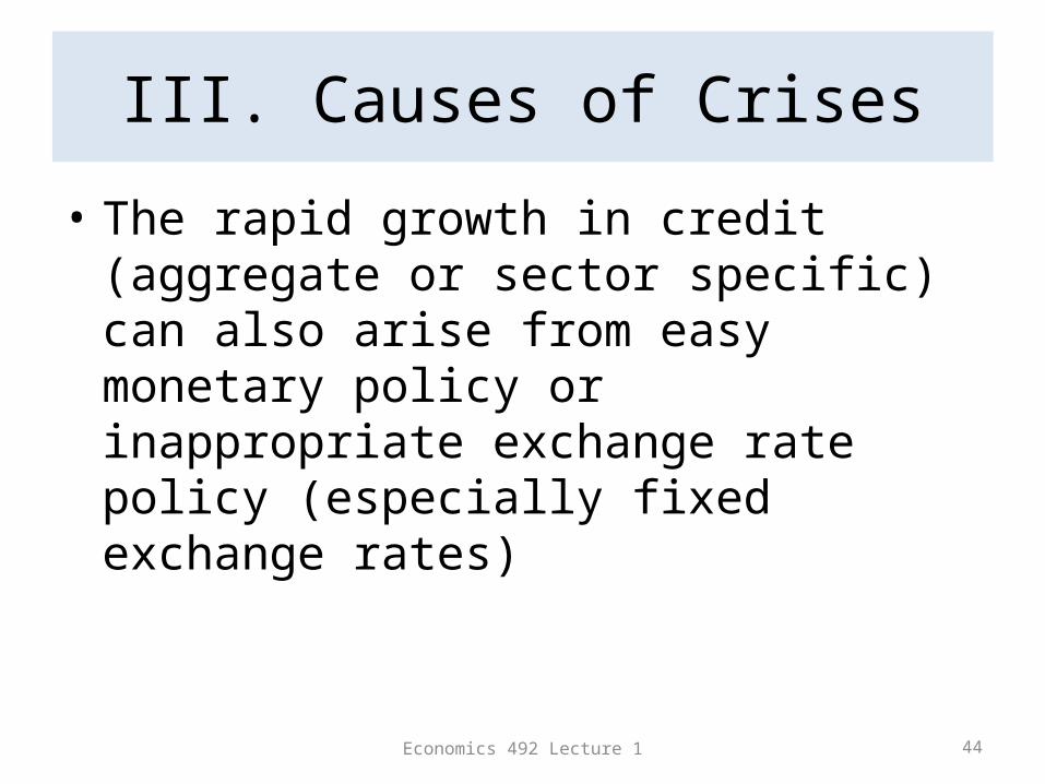
• The rapid growth in credit (aggregate or sector specific) can also arise from easy monetary policy or inappropriate exchange rate policy (especially fixed exchange rates)
Economics 492 Lecture 1 45
III. Causes of Crises
• Note: rapid growth in credit raises leverage, which is the ratio of assets to capital (net worth)
• Leverage is closely related to the following debt ratios:– (for households): debt / personal dispos. income– (for businesses): debt / equity– (for governments): debt / GDP
Economics 492 Lecture 1 46
III. Causes of Crises
• Note: Credit expansion places the emphasis on credit decisions gone bad and the eventual insolvency of banks. When we talk about transmission, we will see that we can’t entirely divorce insolvency from illiquidity. – Banks can become illiquid even if they are solvent– In turn, their illiquidity can lead to their insolvency– Suspicion about solvency, however, is the greatest
cause of illiquidity
Economics 492 Lecture 1 47
III. Causes of Crises
• Asset bubbles are typically a contributing factor to crises. They typically are supported by rapid sectoral credit expansion.– When asset bubbles are not associated with rapid credit
expansion, there is typically less of a problem when they burst because the financial sector is less harmed (banks don’t typically fall).• Example: Tech bubble in late 1990s
– Asset bubbles most common in housing or real estate, and in stock markets (but also exchange markets and commodities)
– Shiller has been a proponent of a psychological effect in the development of bubbles (rejects efficient markets)
Economics 492 Lecture 1 48
III. Causes of Crises
• 7 biggest financial bubbles in last 40 years (KA)– Bank loans to Mexico and other developing countries in the
1970s– Japanese bubble in real estate and stocks in late 1980s– Nordic bubble in real estate and stocks in late 1980s (Finland,
Norway, Sweden)– Asian crisis following bubble in real estate and stocks in
Thailand, Malaysia, Indonesia and others– Capital flows into Mexico in 1990-93– Tech stock bubble in U.S. from 1995-2000– Bubbles in real estate in U.S., U.K., Ireland, Iceland, and
Hungary in early 2000s and the world financial crisis 2007-2009
Economics 492 Lecture 1 49
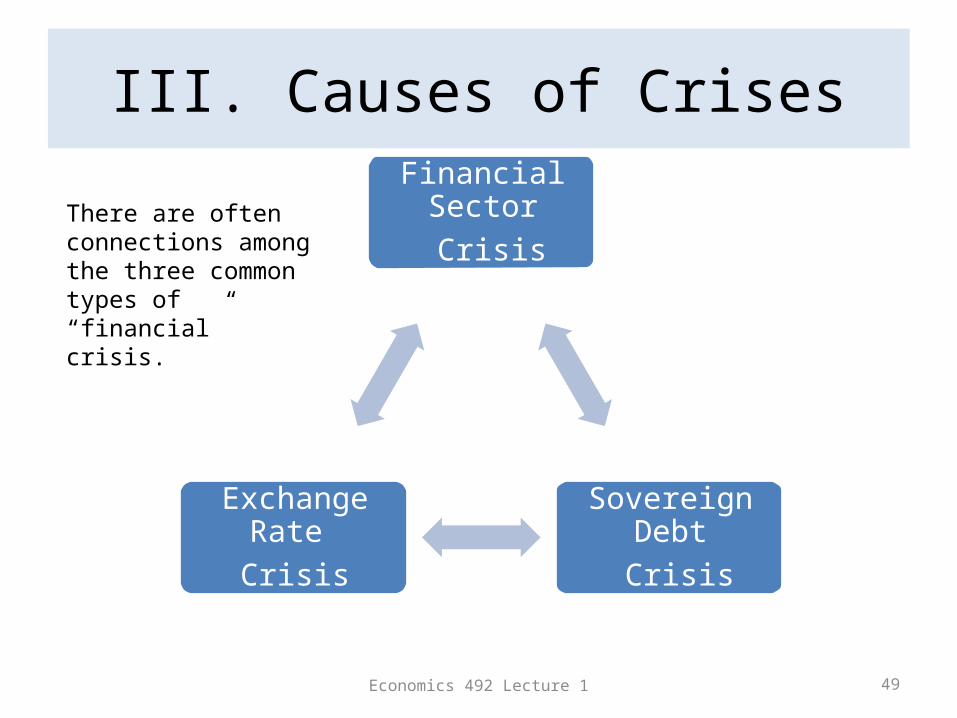
III. Causes of CrisesFinancial Sector
Crisis
Sovereign Debt Crisis
Exchange Rate Crisis
There are often connections among the three common types of “financial” crisis.
Economics 492 Lecture 1 50
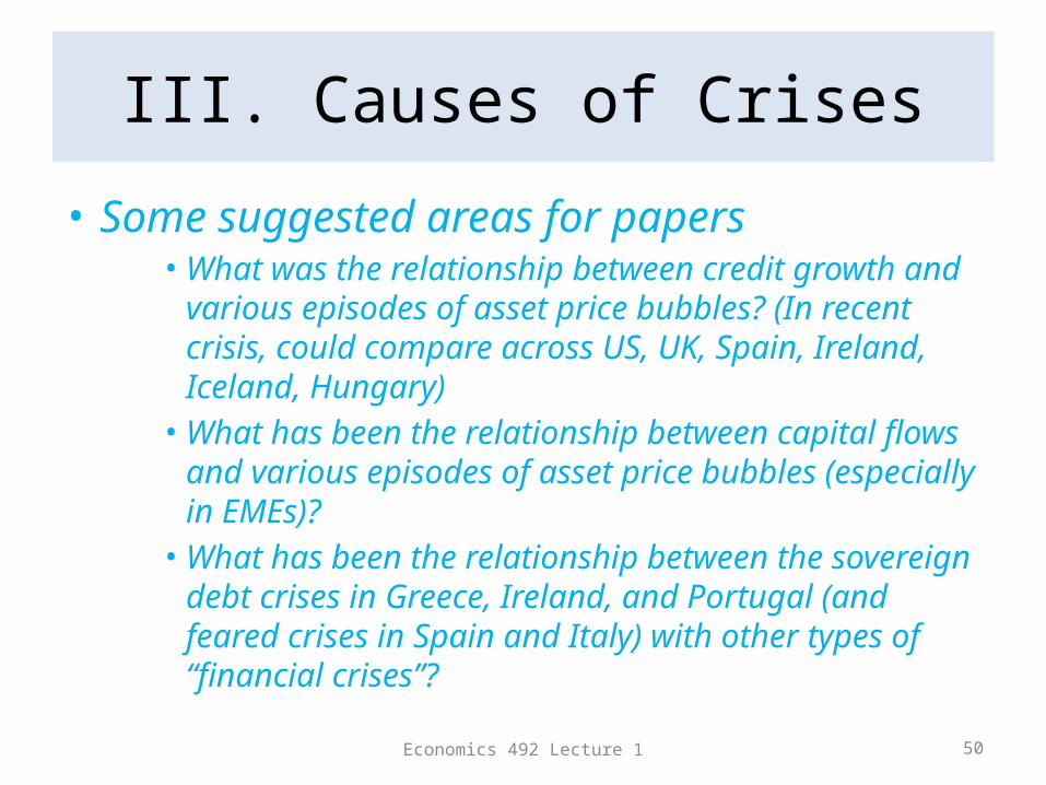
III. Causes of Crises
• Some suggested areas for papers• What was the relationship between credit growth and
various episodes of asset price bubbles? (In recent crisis, could compare across US, UK, Spain, Ireland, Iceland, Hungary)
• What has been the relationship between capital flows and various episodes of asset price bubbles (especially in EMEs)?
• What has been the relationship between the sovereign debt crises in Greece, Ireland, and Portugal (and feared crises in Spain and Italy) with other types of “financial crises”?
Economics 492 Lecture 1 51
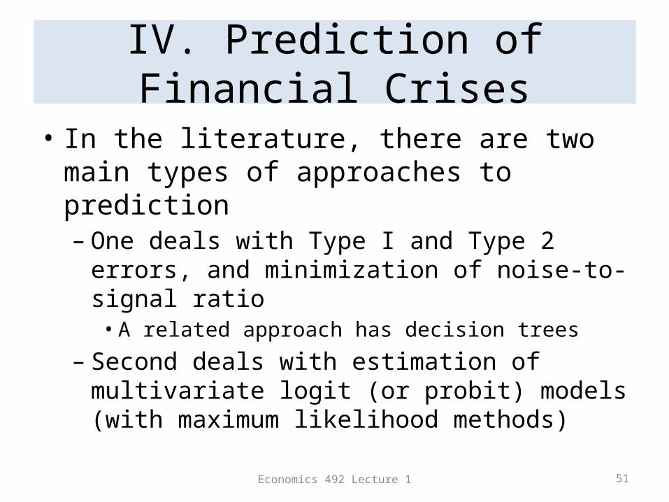
IV. Prediction of Financial Crises
• In the literature, there are two main types of approaches to prediction– One deals with Type I and Type 2 errors, and
minimization of noise-to-signal ratio• A related approach has decision trees
– Second deals with estimation of multivariate logit (or probit) models (with maximum likelihood methods)
Economics 492 Lecture 1 52
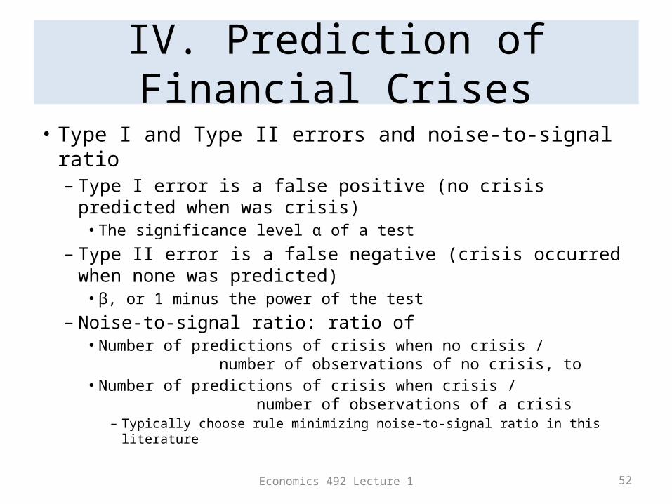
IV. Prediction of Financial Crises
• Type I and Type II errors and noise-to-signal ratio– Type I error is a false positive (no crisis predicted when was
crisis)• The significance level α of a test
– Type II error is a false negative (crisis occurred when none was predicted)• β, or 1 minus the power of the test
– Noise-to-signal ratio: ratio of• Number of predictions of crisis when no crisis / number
of observations of no crisis, to• Number of predictions of crisis when crisis / number
of observations of a crisis– Typically choose rule minimizing noise-to-signal ratio in this literature
Economics 492 Lecture 1 53
IV. Prediction of Financial Crises
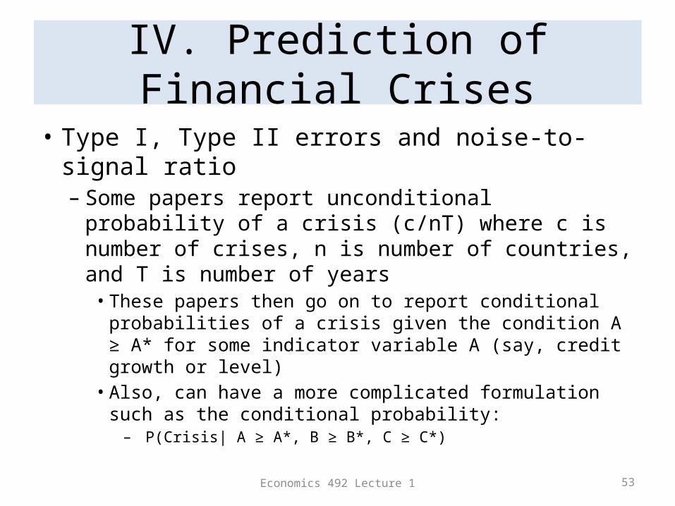
• Type I, Type II errors and noise-to-signal ratio– Some papers report unconditional probability of a
crisis (c/nT) where c is number of crises, n is number of countries, and T is number of years• These papers then go on to report conditional
probabilities of a crisis given the condition A ≥ A* for some indicator variable A (say, credit growth or level)• Also, can have a more complicated formulation such as
the conditional probability:– P(Crisis| A ≥ A*, B ≥ B*, C ≥ C*)
Economics 492 Lecture 1 54
IV. Prediction of Financial Crises
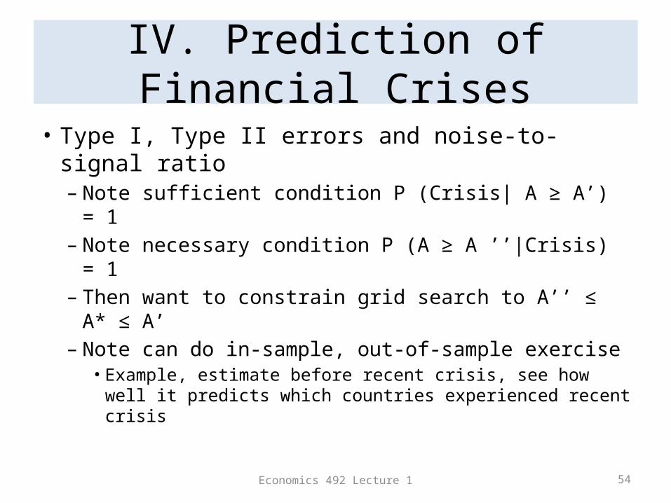
• Type I, Type II errors and noise-to-signal ratio– Note sufficient condition P (Crisis| A ≥ A’) = 1– Note necessary condition P (A ≥ A ’’|Crisis) = 1– Then want to constrain grid search to A’’ ≤ A* ≤ A’– Note can do in-sample, out-of-sample exercise• Example, estimate before recent crisis, see how well it
predicts which countries experienced recent crisis
Economics 492 Lecture 1 55
IV. Prediction of Financial Crises
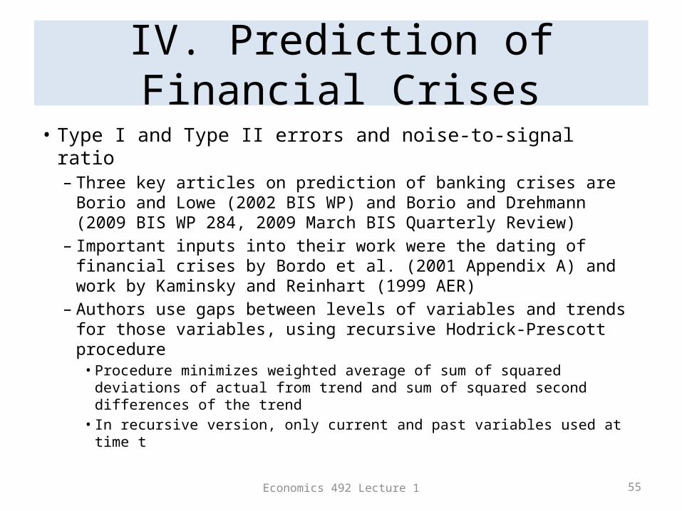
• Type I and Type II errors and noise-to-signal ratio– Three key articles on prediction of banking crises are Borio and
Lowe (2002 BIS WP) and Borio and Drehmann (2009 BIS WP 284, 2009 March BIS Quarterly Review)
– Important inputs into their work were the dating of financial crises by Bordo et al. (2001 Appendix A) and work by Kaminsky and Reinhart (1999 AER)
– Authors use gaps between levels of variables and trends for those variables, using recursive Hodrick-Prescott procedure• Procedure minimizes weighted average of sum of squared deviations
of actual from trend and sum of squared second differences of the trend
• In recursive version, only current and past variables used at time t
Economics 492 Lecture 1 56
IV. Prediction of Financial Crises
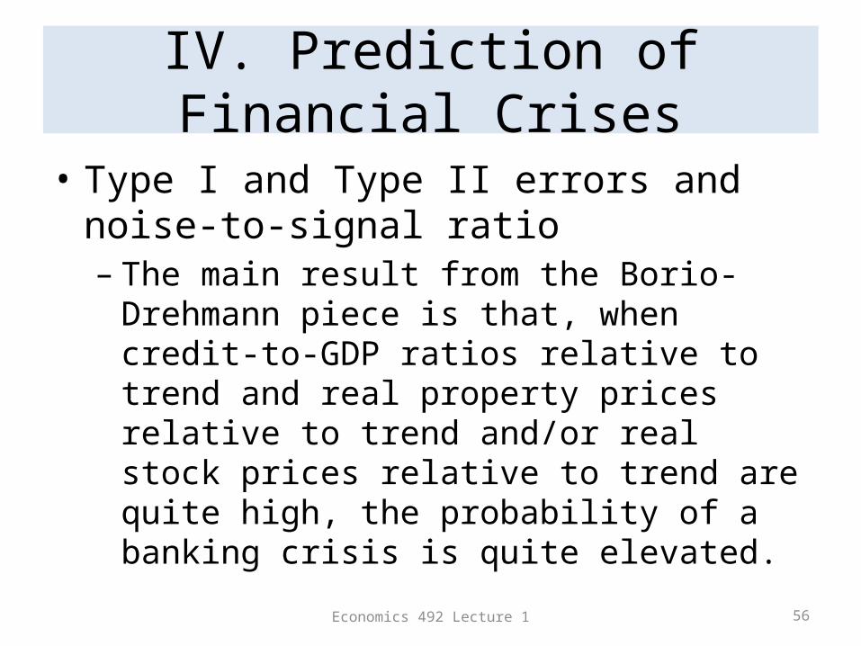
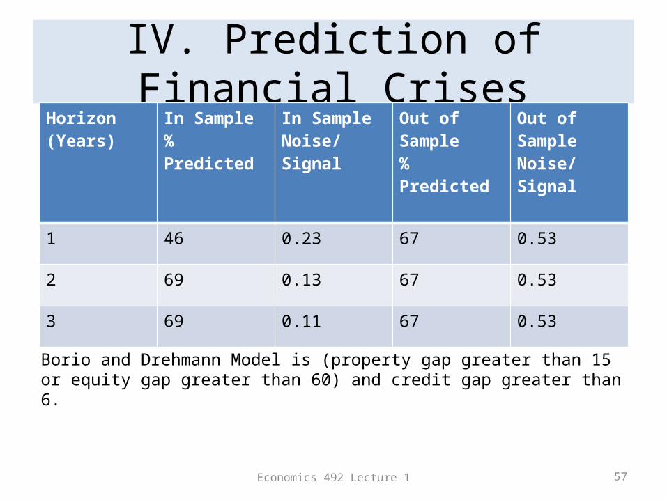
• Type I and Type II errors and noise-to-signal ratio– The main result from the Borio-Drehmann piece is
that, when credit-to-GDP ratios relative to trend and real property prices relative to trend and/or real stock prices relative to trend are quite high, the probability of a banking crisis is quite elevated.
Economics 492 Lecture 1 57
IV. Prediction of Financial CrisesHorizon(Years)
In Sample% Predicted
In SampleNoise/Signal
Out of Sample% Predicted
Out of SampleNoise/Signal
1 46 0.23 67 0.53
2 69 0.13 67 0.53
3 69 0.11 67 0.53
Borio and Drehmann Model is (property gap greater than 15 or equity gap greater than 60) and credit gap greater than 6.
Economics 492 Lecture 1 58
IV. Prediction of Financial Crises
• Logit (or probit) model– Logit model is based on logistic function:
• )• Where + + … + • Note, as (no crisis)• Note , as (crisis)• If larger values of x are associated with a greater chance of crisis then
their coefficients will be positive.
– Probit model is based on the inverse cumulative density function of the standard normal distribution
– (Many feel that practically the differences between probit and logit are not too large. Estimates of multivariate logit tend to converge better/faster than estimates of multivariate probit.)
Economics 492 Lecture 1 59
IV. Prediction of Financial Crises
• Logit– Reinhart-Rogoff show that This time is Not different in many
different dimensions. Reinhart-Rogoff (2011 AER)(logit regressions)• Systemic banking crises in financial centers (U.S., U.K., and historically
France) help explain domestic banking crises• Domestic banking crises help explain sovereign debt defaults• Growth in public debt helps explain sovereign debt defaults• External-debt-to-GDP ratio helps explain banking crises
– Schularick and Taylor (2009 NBER) use logit regressions to show that it is real loan growth, not real money growth, than predicts banking crises historically
– Eichengreen (2004) estimates regressions for exchange rate crises
Economics 492 Lecture 1 60
IV. Prediction of Financial Crises
• Some suggested areas for papers:– Add to Borio and Drehmann an international dimension:
contagion from other crises or assets of domestic banks in foreign countries or …
– In Reinhart and Rogoff (2011) explore whether the inclusion of both external debt ratio and growth in overall public debt changes conclusions about what predicts banking crises and defaults post 1974
– Using estimated equations from various authors, what are the probabilities of sovereign defaults by Spain and Italy and other countries with high or rising debt in 2011-12?
Economics 492 Lecture 1 61
Suggestions for this week• Review Lecture at ECON 492 web site• Skim through Reference List for ECON 492 on ECON 492 web site;
what sparks your interest? Pursue a reference.• Which are the most important financial crises? Read one or two
of:– KA chapters 1-3 (skim the rest)– Reinhart and Rogoff chapters 1, 10, 13 (skim the rest)– Reinhart and Rogoff, “Banking Crises: An Equal Opportunity Measure”– Reinhart and Rogoff, “From Financial Crash to Debt Crisis”– The Squam Lake Report chapter 1
• If you have an idea of what you would like to do already, see me