Embed Size (px)
DESCRIPTION
ECONOMETRICS UBC Stock & Watson CHAPTER 1 - 3
Citation preview

7/21/2019 ECON 491: ECONOMETRICS STOCK AND WATSON PPT
http://slidepdf.com/reader/full/econ-491-econometrics-stock-and-watson-ppt 1/63
Copyright © 2011 Pearson Addison-Wesley. All rights reserved.
UBC OkanaganDr. Mohsen Javdani
Winter 2, 2015/2016
Econ427:Econometrocs
(From Stock and Watson’s Introductionto Econometrics)
Chapters 1,2,3
1-1

7/21/2019 ECON 491: ECONOMETRICS STOCK AND WATSON PPT
http://slidepdf.com/reader/full/econ-491-econometrics-stock-and-watson-ppt 2/63
Copyright © 2011 Pearson Addison-Wesley. All rights reserved. 1-2
Brief Overview of the Course
• Economics suggests important relationships, oftenwith policy implications, but virtually neversuggests quantitative magnitudes of causaleffects.
–
What is the quantitative effect of reducing class size onstudent achievement?
–
How does another year of education change earnings?
–
What is the price elasticity of cigarettes?
–
What is the effect on output growth of a 1 percentage
point increase in interest rates by the Fed?– What is the effect on housing prices of environmental
improvements?

7/21/2019 ECON 491: ECONOMETRICS STOCK AND WATSON PPT
http://slidepdf.com/reader/full/econ-491-econometrics-stock-and-watson-ppt 3/63
Copyright © 2011 Pearson Addison-Wesley. All rights reserved. 1-3
This course is about using data tomeasure causal effects.
•
Ideally, we would like an experiment– What would be an experiment to estimate the effect of class
size on standardized test scores?
•
But almost always we only have observational(nonexperimental) data.
–
returns to education– cigarette prices
– monetary policy
• Most of the course deals with difficulties arising from usingobservational data to estimate causal effects
–
confounding effects (omitted factors)– simultaneous causality
– “correlation does not imply causation”

7/21/2019 ECON 491: ECONOMETRICS STOCK AND WATSON PPT
http://slidepdf.com/reader/full/econ-491-econometrics-stock-and-watson-ppt 4/63
Copyright © 2011 Pearson Addison-Wesley. All rights reserved. 1-4
• Learn methods for estimating causal effects usingobservational data
• Learn some tools that can be used for other purposes; forexample, forecasting using time series data;
•
Focus on applications – theory is used only as needed tounderstand the whys of the methods;
•
Learn to evaluate the regression analysis of others – thismeans you will be able to read/understand empiricaleconomics papers in other econ courses;
•
Get some hands-on experience with regression analysis inyour problem sets.
In this course you will:
7/21/2019 ECON 491: ECONOMETRICS STOCK AND WATSON PPT
http://slidepdf.com/reader/full/econ-491-econometrics-stock-and-watson-ppt 5/63
Copyright © 2011 Pearson Addison-Wesley. All rights reserved. 1-5
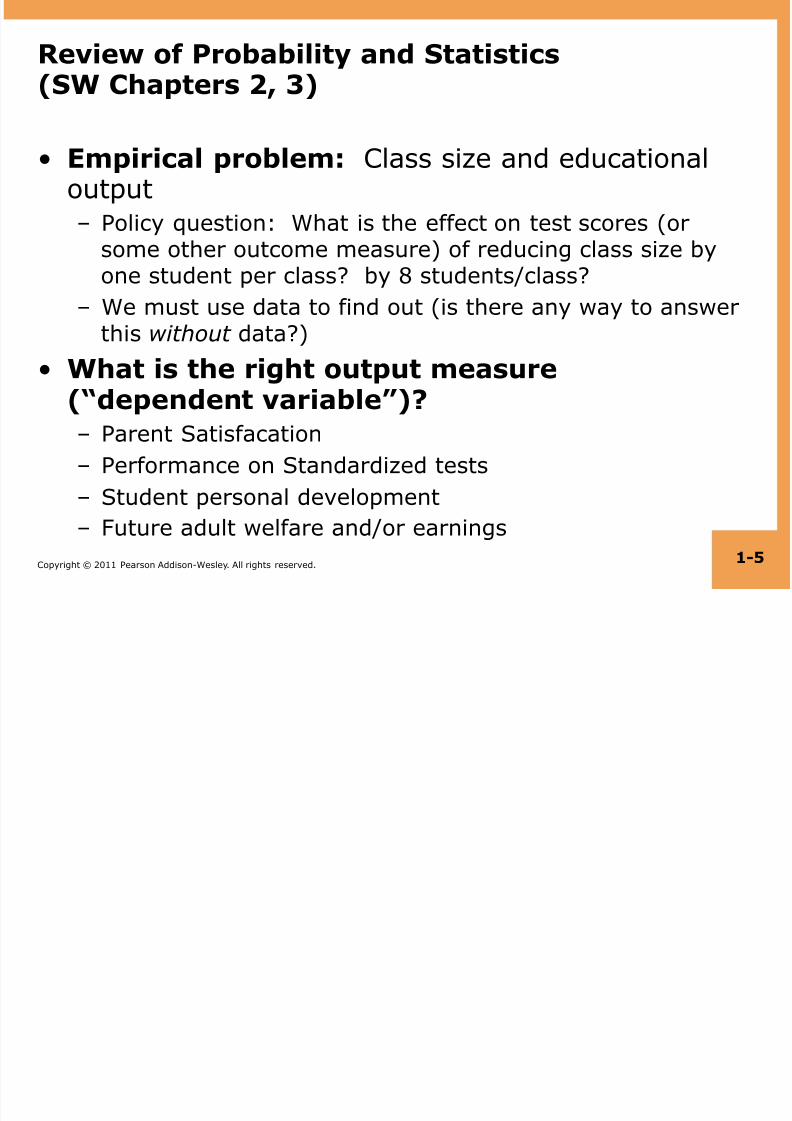
• Empirical problem: Class size and educationaloutput
– Policy question: What is the effect on test scores (orsome other outcome measure) of reducing class size by
one student per class? by 8 students/class? –
We must use data to find out (is there any way to answerthis without data?)
• What is the right output measure(“dependent variable”)?
– Parent Satisfacation
–
Performance on Standardized tests
–
Student personal development
– Future adult welfare and/or earnings
Review of Probability and Statistics(SW Chapters 2, 3)

7/21/2019 ECON 491: ECONOMETRICS STOCK AND WATSON PPT
http://slidepdf.com/reader/full/econ-491-econometrics-stock-and-watson-ppt 6/63
Copyright © 2011 Pearson Addison-Wesley. All rights reserved. 1-6
The California Test Score Data Set
All K-6 and K-8 California school districts (n = 420)
Variables:
•
5th
grade test scores (Stanford-9 achievement test,combined math and reading), district average
•
Student-teacher ratio (STR) = no. of students in thedistrict divided by no. full-time equivalent teachers

7/21/2019 ECON 491: ECONOMETRICS STOCK AND WATSON PPT
http://slidepdf.com/reader/full/econ-491-econometrics-stock-and-watson-ppt 7/63
Copyright © 2011 Pearson Addison-Wesley. All rights reserved. 1-7
Initial look at the data:(You should already know how to interpret this table)
This table doesn’t tell us anything about the relationshipbetween test scores and the STR.

7/21/2019 ECON 491: ECONOMETRICS STOCK AND WATSON PPT
http://slidepdf.com/reader/full/econ-491-econometrics-stock-and-watson-ppt 8/63
Copyright © 2011 Pearson Addison-Wesley. All rights reserved. 1-8
Do districts with smaller classes havehigher test scores?
Scatterplot of test score v. student-teacher ratio
What does this figure show?

7/21/2019 ECON 491: ECONOMETRICS STOCK AND WATSON PPT
http://slidepdf.com/reader/full/econ-491-econometrics-stock-and-watson-ppt 9/63
Copyright © 2011 Pearson Addison-Wesley. All rights reserved. 1-9
We need to get some numerical evidence on whetherdistricts with low STRs have higher test scores – but how?
1.
Compare average test scores in districts with low STRs to
those with high STRs (“estimation”)
2.
Test the “null” hypothesis that the mean test scores in the
two types of districts are the same, against the
alternative” hypothesis that they differ (“hypothesistesting”)
3.
Estimate an interval for the difference in the mean test
scores, high v. low STR districts (“confidence interval ”)

7/21/2019 ECON 491: ECONOMETRICS STOCK AND WATSON PPT
http://slidepdf.com/reader/full/econ-491-econometrics-stock-and-watson-ppt 10/63
Copyright © 2011 Pearson Addison-Wesley. All rights reserved. 1-10
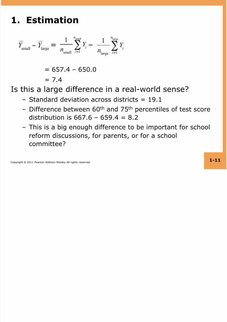
Initial data analysis: Compare districts with small” (STR < 20)and large” (STR ! 20) class sizes:
1. Estimation of ! = difference between group means
2. Test the hypothesis that ! = 0
3. Construct a confidence interval for !
Class Size Average score( )
Standard deviation(sBY B)
n
Small 657.4 19.4 238
Large 650.0 17.9 182
Y
7/21/2019 ECON 491: ECONOMETRICS STOCK AND WATSON PPT
http://slidepdf.com/reader/full/econ-491-econometrics-stock-and-watson-ppt 11/63
Copyright © 2011 Pearson Addison-Wesley. All rights reserved. 1-11
1. Estimation
= –
= 657.4 – 650.0
= 7.4Is this a large difference in a real-world sense?
– Standard deviation across districts = 19.1
– Difference between 60th and 75th percentiles of test score
distribution is 667.6 – 659.4 = 8.2– This is a big enough difference to be important for school
reform discussions, for parents, or for a school
committee?
1
nsmall
Y i
i=1
nsmall
! Y small
! Y large
1n
large
Y i
i=1
n
large
!
7/21/2019 ECON 491: ECONOMETRICS STOCK AND WATSON PPT
http://slidepdf.com/reader/full/econ-491-econometrics-stock-and-watson-ppt 12/63
Copyright © 2011 Pearson Addison-Wesley. All rights reserved. 1-12
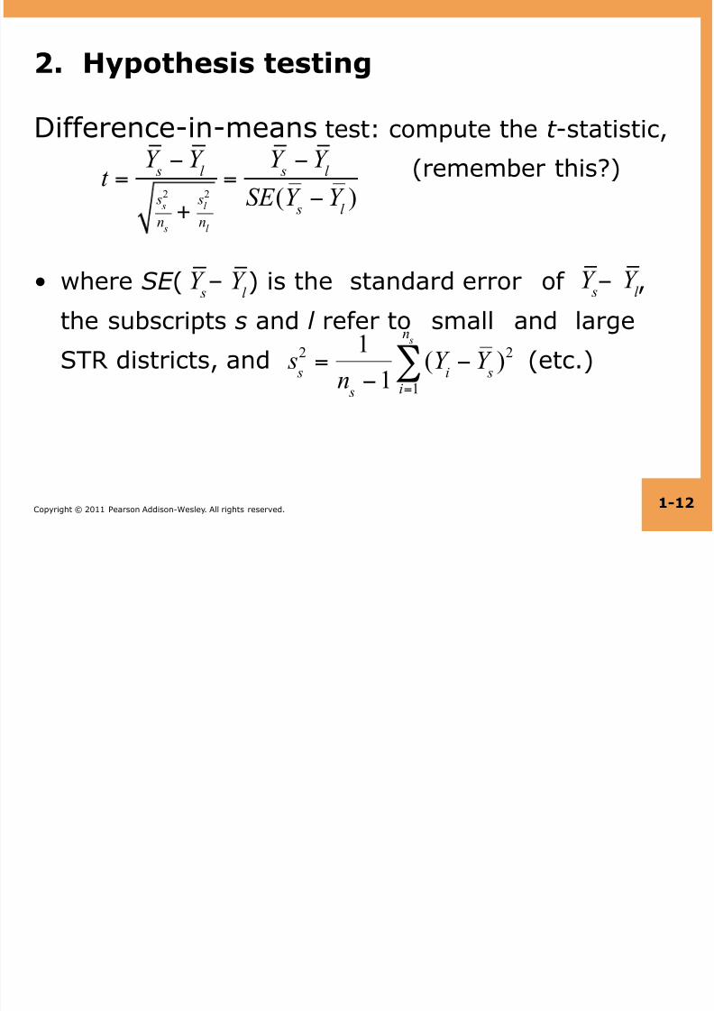
2. Hypothesis testing
t =Y s !Y
l
s s
2
n s
+ s
l
2
nl
=
Y s !Y
l
SE (Y s !Y
l )
Difference-in-means test: compute the t -statistic, (remember this?)
• where SE ( – ) is the standard error” of – ,
the subscripts s and l refer to “small” and large”
STR districts, and (etc.)
Y s
Y l
Y s
Y l
s s
2=
1
n s !1(Y
i
!Y s
)2
i=1
n s
"

7/21/2019 ECON 491: ECONOMETRICS STOCK AND WATSON PPT
http://slidepdf.com/reader/full/econ-491-econometrics-stock-and-watson-ppt 13/63
Copyright © 2011 Pearson Addison-Wesley. All rights reserved. 1-13
Compute the difference-of-means t -statistic:
= 4.05
|t| > 1.96, so reject (at the 5% significance level)the null hypothesis that the two means are thesame.
Size sY n small 657.4 19.4 238
large 650.0 17.9 182
Y
t =Y s !
Y l
s s
2
n s
+ s
l
2
nl
=
657.4!650.0
19.42
238 +
17.92
182
=
7.4
1.83

7/21/2019 ECON 491: ECONOMETRICS STOCK AND WATSON PPT
http://slidepdf.com/reader/full/econ-491-econometrics-stock-and-watson-ppt 14/63
Copyright © 2011 Pearson Addison-Wesley. All rights reserved. 1-14
3. Confidence interval
A 95% confidence interval for the difference betweenthe means is,
( – ) ± 1.96"SE ( – )
= 7.4 ± 1.96"1.83 = (3.8, 11.0)
Two equivalent statements:1. The 95% confidence interval for ! doesn’t include 0;
2. The hypothesis that ! = 0 is rejected at the 5% level.
Y l
Y s
Y l
Y s

7/21/2019 ECON 491: ECONOMETRICS STOCK AND WATSON PPT
http://slidepdf.com/reader/full/econ-491-econometrics-stock-and-watson-ppt 15/63
Copyright © 2011 Pearson Addison-Wesley. All rights reserved. 1-15
What comes next…
•
The mechanics of estimation, hypothesis testing,and confidence intervals should be familiar
• These concepts extend directly to regression andits variants
•
Before turning to regression, however, we willreview some of the underlying theory ofestimation, hypothesis testing, and confidenceintervals:– Why do these procedures work, and why use these rather
than others?– We will review the intellectual foundations of statistics
and econometrics
7/21/2019 ECON 491: ECONOMETRICS STOCK AND WATSON PPT
http://slidepdf.com/reader/full/econ-491-econometrics-stock-and-watson-ppt 16/63
Copyright © 2011 Pearson Addison-Wesley. All rights reserved. 1-16
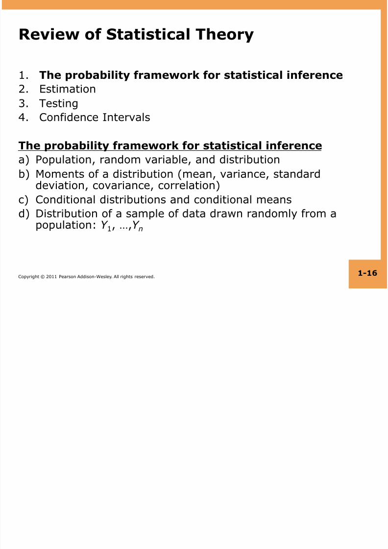
Review of Statistical Theory
1.
The probability framework for statistical inference
2. Estimation
3.
Testing
4. Confidence Intervals
The probability framework for statistical inference
a) Population, random variable, and distribution
b) Moments of a distribution (mean, variance, standarddeviation, covariance, correlation)
c)
Conditional distributions and conditional meansd)
Distribution of a sample of data drawn randomly from apopulation: Y 1, …,Y n

7/21/2019 ECON 491: ECONOMETRICS STOCK AND WATSON PPT
http://slidepdf.com/reader/full/econ-491-econometrics-stock-and-watson-ppt 17/63
Copyright © 2011 Pearson Addison-Wesley. All rights reserved. 1-17
(a) Population, random variable, anddistribution
Population
•
The group or collection of all possible entities of interest(school districts)
• We will think of populations as infinitely large (# is an
approximation to“very big
”)
Random variable Y
•
Numerical summary of a random outcome (district averagetest score, district STR)

7/21/2019 ECON 491: ECONOMETRICS STOCK AND WATSON PPT
http://slidepdf.com/reader/full/econ-491-econometrics-stock-and-watson-ppt 18/63
Copyright © 2011 Pearson Addison-Wesley. All rights reserved. 1-18
Population distribution of Y
• The probabilities of different values of Y that occurin the population, for ex. Pr[Y = 650] (when Y isdiscrete)
• or: The probabilities of sets of these values, forex. Pr[640 $ Y $ 660] (when Y is continuous).

7/21/2019 ECON 491: ECONOMETRICS STOCK AND WATSON PPT
http://slidepdf.com/reader/full/econ-491-econometrics-stock-and-watson-ppt 19/63
Copyright © 2011 Pearson Addison-Wesley. All rights reserved. 1-19
(b) Moments of a population distribution: mean,variance, standard deviation, covariance,correlation
mean = expected value (expectation) of Y
= E (Y )
= ! Y
= long-run average value of Y over repeatedrealizations of Y
variance = E (Y – ! Y )2
=
= measure of the squared spread ofthe distribution
standard deviation = = " Y
! Y
2
variance

7/21/2019 ECON 491: ECONOMETRICS STOCK AND WATSON PPT
http://slidepdf.com/reader/full/econ-491-econometrics-stock-and-watson-ppt 20/63
Copyright © 2011 Pearson Addison-Wesley. All rights reserved. 1-20
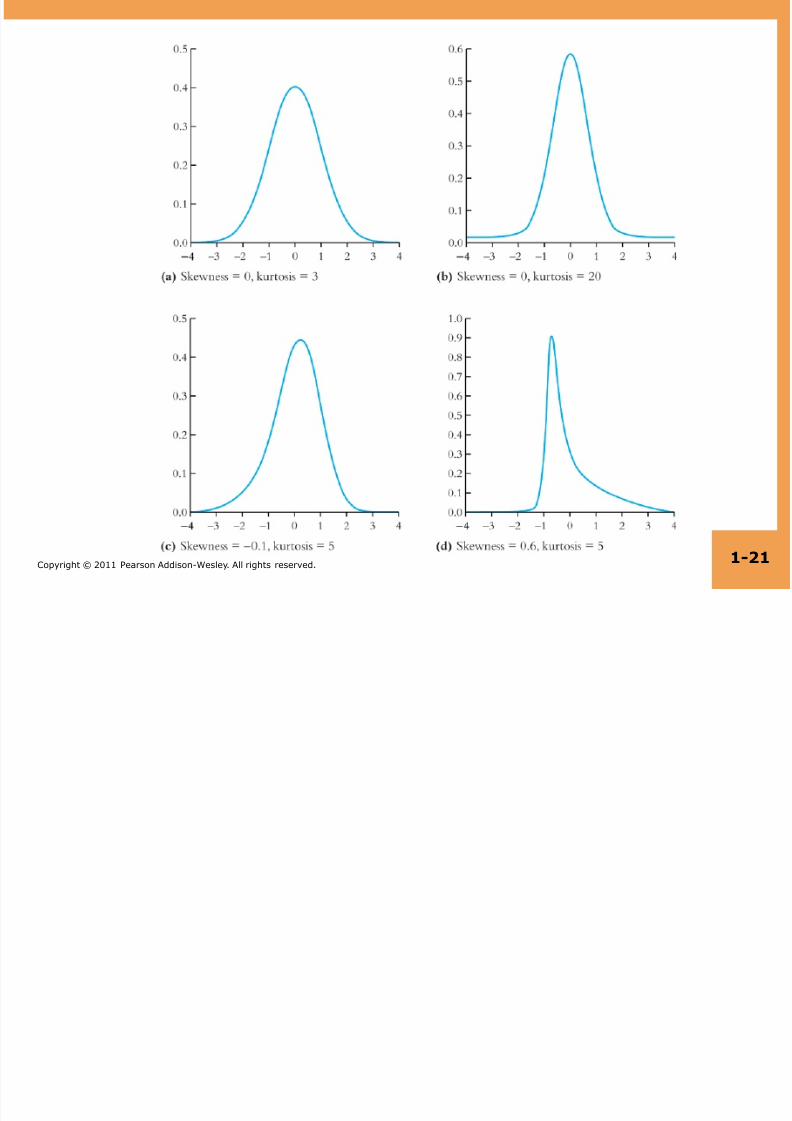
Moments, ctd.
skewness =
= measure of asymmetry of a distribution
•
skewness = 0: distribution is symmetric
• skewness > (<) 0: distribution has long right (left) tail
kurtosis =
= measure of mass in tails
= measure of probability of large values•
kurtosis = 3: normal distribution
•
skewness > 3: heavy tails (“leptokurtotic
)
E Y ! µ Y
( )
3"
#$
%
&'(
Y
3
E Y ! µ Y
( )4"
#$%&'
( Y
4
7/21/2019 ECON 491: ECONOMETRICS STOCK AND WATSON PPT
http://slidepdf.com/reader/full/econ-491-econometrics-stock-and-watson-ppt 21/63
Copyright © 2011 Pearson Addison-Wesley. All rights reserved. 1-21

7/21/2019 ECON 491: ECONOMETRICS STOCK AND WATSON PPT
http://slidepdf.com/reader/full/econ-491-econometrics-stock-and-watson-ppt 22/63
Copyright © 2011 Pearson Addison-Wesley. All rights reserved. 1-22
2 random variables: joint distributionsand covariance
• Random variables X and Z have a joint distribution
•
The covariance between X and Z is
– cov( X ,Z ) = E [( X – ! X )(Z – ! Z )] = " XZ
• The covariance is a measure of the linear association
between X and Z ; its units are units of X "units of Z
•
cov( X ,Z ) > 0 means a positive relation between X and Z
•
If X and Z are independently distributed, then cov( X ,Z ) = 0(but not vice versa!!)
•
The covariance of a r.v. with itself is its variance:
cov( X , X ) = E [( X – ! B X B)( X – ! B X B)] = E [( X – ! X )2] =!
X
2
7/21/2019 ECON 491: ECONOMETRICS STOCK AND WATSON PPT
http://slidepdf.com/reader/full/econ-491-econometrics-stock-and-watson-ppt 23/63
Copyright © 2011 Pearson Addison-Wesley. All rights reserved. 1-23
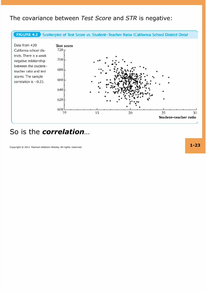
The covariance between Test Score and STR is negative:
So is the correlation…

7/21/2019 ECON 491: ECONOMETRICS STOCK AND WATSON PPT
http://slidepdf.com/reader/full/econ-491-econometrics-stock-and-watson-ppt 24/63
Copyright © 2011 Pearson Addison-Wesley. All rights reserved. 1-24
The correlation coefficient is defined in terms ofthe covariance:
corr( X ,Z ) = = r XZ
• –1 $ corr( X ,Z ) $ 1
•
corr( X ,Z ) = 1 mean perfect positive linear association•
corr( X ,Z ) = –1 means perfect negative linear association
• corr( X ,Z ) = 0 means no linear association
cov( X , Z )
var( X )var( Z )=
! XZ
! X !
Z

7/21/2019 ECON 491: ECONOMETRICS STOCK AND WATSON PPT
http://slidepdf.com/reader/full/econ-491-econometrics-stock-and-watson-ppt 25/63
Copyright © 2011 Pearson Addison-Wesley. All rights reserved. 1-25
The correlation coefficient measures linearassociation

7/21/2019 ECON 491: ECONOMETRICS STOCK AND WATSON PPT
http://slidepdf.com/reader/full/econ-491-econometrics-stock-and-watson-ppt 26/63
Copyright © 2011 Pearson Addison-Wesley. All rights reserved. 1-26
(c) Conditional distributions andconditional means
Conditional distributions
•
The distribution of Y , given value(s) of some other randomvariable, X
• Ex: the distribution of test scores, given that STR < 20
Conditional expectations and conditional moments•
conditional mean = mean of conditional distribution
– = E (Y | X = x ) (important concept and notation)
• conditional variance = variance of conditional distribution
•
Example: E (Test scores|STR < 20) = the mean of test
scores among districts with small class sizes
The difference in means is the difference between themeans of two conditional distributions:

7/21/2019 ECON 491: ECONOMETRICS STOCK AND WATSON PPT
http://slidepdf.com/reader/full/econ-491-econometrics-stock-and-watson-ppt 27/63
Copyright © 2011 Pearson Addison-Wesley. All rights reserved. 1-27
Conditional mean, ctd.
! = E (Test scores|STR < 20) – E (Test scores|STR ! 20)
Other examples of conditional means:
•
Wages of all female workers (Y = wages, X = gender)
•
Mortality rate of those given an experimental treatment (Y =live/die; X = treated/not treated)
•
If E ( X |Z ) = const, then corr( X ,Z ) = 0 (not necessarily viceversa however)
The conditional mean is a (possibly new) term for thefamiliar idea of the group mean

7/21/2019 ECON 491: ECONOMETRICS STOCK AND WATSON PPT
http://slidepdf.com/reader/full/econ-491-econometrics-stock-and-watson-ppt 28/63
Copyright © 2011 Pearson Addison-Wesley. All rights reserved. 1-28
(d) Distribution of a sample of data drawnrandomly from a population: Y 1,…, Y n
We will assume simple random sampling
•
Choose and individual (district, entity) at random from thepopulation
Randomness and data
•
Prior to sample selection, the value of Y is random becausethe individual selected is random
• Once the individual is selected and the value of Y isobserved, then Y is just a number – not random
• The data set is (Y 1, Y 2,…, Y n), where Y i = value of Y for the i th
individual (district, entity) sampled

7/21/2019 ECON 491: ECONOMETRICS STOCK AND WATSON PPT
http://slidepdf.com/reader/full/econ-491-econometrics-stock-and-watson-ppt 29/63
Copyright © 2011 Pearson Addison-Wesley. All rights reserved. 1-29
Distribution of Y B1B,…, Y BnB under simplerandom sampling
•
Because individuals #1 and #2 are selected atrandom, the value of Y 1 has no informationcontent for Y 2. Thus:
– Y 1 and Y 2 are independently distributed
–
Y 1 and Y 2 come from the same distribution, that is, Y 1, Y 2 are identically distributed
–
That is, under simple random sampling, Y 1 and Y 2 areindependently and identically distributed (i.i.d.).
– More generally, under simple random sampling, {Y i }, i =
1,…, n, are i.i.d.

7/21/2019 ECON 491: ECONOMETRICS STOCK AND WATSON PPT
http://slidepdf.com/reader/full/econ-491-econometrics-stock-and-watson-ppt 30/63
Copyright © 2011 Pearson Addison-Wesley. All rights reserved. 1-30
This framework allows rigorous statistical inferencesabout moments of population distributions using a sampleof data from that population …
1.
The probability framework for statistical inference
2. Estimation
3.
Testing
4. Confidence Intervals
Estimation
is the natural estimator of the mean. But:
a) What are the properties of ?
b) Why should we use rather than some other estimator?
•
Y 1 (the first observation)
• maybe unequal weights – not simple average
•
median(Y 1,…, Y n)
The starting point is the sampling distribution of …
Y
Y
Y
Y

7/21/2019 ECON 491: ECONOMETRICS STOCK AND WATSON PPT
http://slidepdf.com/reader/full/econ-491-econometrics-stock-and-watson-ppt 31/63
Copyright © 2011 Pearson Addison-Wesley. All rights reserved. 1-31
(a) The sampling distribution of
is a random variable, and its properties aredetermined by the sampling distribution of
– The individuals in the sample are drawn at random.
–
Thus the values of (Y 1, …, Y n) are random
–
Thus functions of (Y 1, …, Y n), such as , are random:had a different sample been drawn, they would havetaken on a different value
–
The distribution of over different possible samples ofsize n is called the sampling distribution of .
–
The mean and variance of are the mean and varianceof its sampling distribution, E ( ) and var( ).
– The concept of the sampling distribution underpins all ofeconometrics.
Y
Y
Y
Y
Y
Y
Y Y
Y

7/21/2019 ECON 491: ECONOMETRICS STOCK AND WATSON PPT
http://slidepdf.com/reader/full/econ-491-econometrics-stock-and-watson-ppt 32/63
Copyright © 2011 Pearson Addison-Wesley. All rights reserved. 1-32
The sampling distribution of , ctd.
Example: Suppose Y takes on 0 or 1 (a Bernoulli randomvariable) with the probability distribution,
Pr[Y = 0] = .22, Pr(Y =1) = .78
Then
E (Y ) = p"
1 + (1 – p)"
0 = p = .78= E [Y – E (Y )]2 = p(1 – p) [remember this?]
= .78" (1–.78) = 0.1716
The sampling distribution of depends on n.
Consider n = 2. The sampling distribution of is,
–
Pr( = 0) = .222 = .0484
– Pr( = ") = 2".22".78 = .3432
– Pr( = 1) = .782 = .6084
Y
! Y
2
Y
Y
Y
Y
Y

7/21/2019 ECON 491: ECONOMETRICS STOCK AND WATSON PPT
http://slidepdf.com/reader/full/econ-491-econometrics-stock-and-watson-ppt 33/63
Copyright © 2011 Pearson Addison-Wesley. All rights reserved. 1-33
The sampling distribution of when Y is Bernoulli ( p = .78):
Y

7/21/2019 ECON 491: ECONOMETRICS STOCK AND WATSON PPT
http://slidepdf.com/reader/full/econ-491-econometrics-stock-and-watson-ppt 34/63
Copyright © 2011 Pearson Addison-Wesley. All rights reserved. 1-34
Things we want to know about thesampling distribution:
•
What is the mean of ?–
If E ( ) = true ! = .78, then is an unbiased estimator of !
• What is the variance of ?
–
How does var( ) depend on n (famous 1/n formula)
• Does become close to ! when n is large?
–
Law of large numbers: is a consistent estimator of !
• – ! appears bell shaped for n large…is this
generally true?–
In fact, – ! is approximately normally distributed for n large (Central Limit Theorem)
Y
Y
Y
Y
Y
Y
Y
Y
Y

7/21/2019 ECON 491: ECONOMETRICS STOCK AND WATSON PPT
http://slidepdf.com/reader/full/econ-491-econometrics-stock-and-watson-ppt 35/63
Copyright © 2011 Pearson Addison-Wesley. All rights reserved. 1-35
The mean and variance of the samplingdistribution of
•
General case – that is, for Y i i.i.d. from any distribution, not just Bernoulli:
• mean: E ( ) = E ( ) = = = ! Y
•
Variance: var( ) = E [ – E ( )]2
= E [ – ! Y ]2
= E
= E
Y
Y
1
nY
i
i=1
n
!
1
n E (Y
i)
i=1
n
!
1
nµ
Y
i=1
n
!
Y Y Y
1
n
Y i
i=1
n
!"
#$
%
&' ( µ
Y
)
*+
,
-.
2
1
n(Y
i ! µ
Y )
i=1
n
"#
$%
&
'(
2
Y

7/21/2019 ECON 491: ECONOMETRICS STOCK AND WATSON PPT
http://slidepdf.com/reader/full/econ-491-econometrics-stock-and-watson-ppt 36/63
Copyright © 2011 Pearson Addison-Wesley. All rights reserved. 1-36
so var( ) = E
=
=
=
=
=
1
n(Y
i ! µ
Y )
i=1
n
"#
$%
&
'(
2
Y
E 1
n(Y
i ! µ
Y )
i=1
n
"#
$%
&
'( )
1
n(Y
j ! µ
Y )
j=1
n
"#
$%
&
'(
*+,
,
./,
,
1
n2
E (Y i ! µ
Y )(Y
j ! µ
Y )"
#
$
% j=1
n
&i=1
n
&
1
n2
cov(Y i,Y
j)
j=1
n
!i=1
n
!
1
n2 ! Y
2
i=1
n
"2
Y
n
!

7/21/2019 ECON 491: ECONOMETRICS STOCK AND WATSON PPT
http://slidepdf.com/reader/full/econ-491-econometrics-stock-and-watson-ppt 37/63
Copyright © 2011 Pearson Addison-Wesley. All rights reserved. 1-37
Mean and variance of samplingdistribution of , ctd.
E ( ) = ! Y
var( ) =
Implications:1. is an unbiased estimator of ! Y (that is, E ( ) = ! Y )
2.
var( ) is inversely proportional to n
1. the spread of the sampling distribution isproportional to 1/
2.
Thus the sampling uncertainty associated withis proportional to 1/ (larger samples, lessuncertainty, but square-root law)
Y
Y
Y
! Y
2
n
Y
Y
Y
n
n
Y

7/21/2019 ECON 491: ECONOMETRICS STOCK AND WATSON PPT
http://slidepdf.com/reader/full/econ-491-econometrics-stock-and-watson-ppt 38/63
Copyright © 2011 Pearson Addison-Wesley. All rights reserved. 1-38
The sampling distribution of when n islarge
For small sample sizes, the distribution of iscomplicated, but if n is large, the samplingdistribution is simple!
1. As n increases, the distribution of becomes more
tightly centered around ! Y (the Law of Large Numbers)2. Moreover, the distribution of – ! Y becomes normal
(the Central Limit Theorem)
Y
Y
Y
Y

7/21/2019 ECON 491: ECONOMETRICS STOCK AND WATSON PPT
http://slidepdf.com/reader/full/econ-491-econometrics-stock-and-watson-ppt 39/63
Copyright © 2011 Pearson Addison-Wesley. All rights reserved. 1-39
The Law of Large Numbers:
An estimator is consistent if the probability that its falls withinan interval of the true population value tends to one as thesample size increases.
If (Y 1,…,Y n) are i.i.d. and < #, then is a consistentestimator of ! Y , that is,
Pr[| – ! Y | < # ] ! 1 as n ! #
which can be written, ! Y
(“ ! Y ” means “ converges in probability to ! Y ”).
(the math: as n ! #, var( ) = ! 0, which implies thatPr[| – ! Y | < # ] ! 1.)
! Y
2Y
Y
!
p
Y
Y
Y
!
p
Y
! Y
2
nY

7/21/2019 ECON 491: ECONOMETRICS STOCK AND WATSON PPT
http://slidepdf.com/reader/full/econ-491-econometrics-stock-and-watson-ppt 40/63
Copyright © 2011 Pearson Addison-Wesley. All rights reserved. 1-40
The Central Limit Theorem (CLT):
If (Y 1,…,Y n) are i.i.d. and 0 < < # , then when n islarge the distribution of is well approximated bya normal distribution.
– is approximately distributed N (! Y , ) (normal
distribution with mean ! Y and variance /n”)
– ( – ! Y )/" Y is Y approximately distributed N (0,1)(standard normal)
– That is, standardized = = is
approximately distributed as N (0,1)
– The larger is n, the better is the approximation.
n Y
! Y
2
Y
Y
! Y
2
n
!
Y
2
Y
Y ! E (Y )
var(Y )
Y ! µ Y
" Y / n

7/21/2019 ECON 491: ECONOMETRICS STOCK AND WATSON PPT
http://slidepdf.com/reader/full/econ-491-econometrics-stock-and-watson-ppt 41/63
Copyright © 2011 Pearson Addison-Wesley. All rights reserved. 1-41
Sampling distribution of when Y is Bernoulli, p = 0.78:
Y

7/21/2019 ECON 491: ECONOMETRICS STOCK AND WATSON PPT
http://slidepdf.com/reader/full/econ-491-econometrics-stock-and-watson-ppt 42/63
Copyright © 2011 Pearson Addison-Wesley. All rights reserved. 1-42
Same example: sampling distribution of :Y ! E (Y )
var(Y )

7/21/2019 ECON 491: ECONOMETRICS STOCK AND WATSON PPT
http://slidepdf.com/reader/full/econ-491-econometrics-stock-and-watson-ppt 43/63
Copyright © 2011 Pearson Addison-Wesley. All rights reserved. 1-43
Summary: The Sampling Distribution of
For Y 1,…,Y n i.i.d. with 0 < < #,
•
The exact (finite sample) sampling distribution of has mean! Y (“ is an unbiased estimator of ! Y ”) and variance /n
• Other than its mean and variance, the exact distribution ofis complicated and depends on the distribution of Y (thepopulation distribution)
•
When n is large, the sampling distribution simplifies:
Y
! Y
2
Y
! Y
2
Y
–
µY (Law of large numbers) !
p
Y
Y ! E (Y )
var(Y )– is approximately N (0,1) (CLT)
Y

7/21/2019 ECON 491: ECONOMETRICS STOCK AND WATSON PPT
http://slidepdf.com/reader/full/econ-491-econometrics-stock-and-watson-ppt 44/63
Copyright © 2011 Pearson Addison-Wesley. All rights reserved. 1-44
(b) Why Use To Estimate ! Y ?
•
is unbiased: E ( ) = ! Y • is consistent: ! Y
• is the least squares” estimator of ! Y ; solves,
so, minimizes the sum of squared residuals”
optional derivation (also see App. 3.2)
= =Set derivative to zero and denote optimal value of m by :
= = or = =
Y
Y
Y
Y
Y
Y !
p
Y
Y
minm
(Y i
! m)2
i=1
n
"
d
dm
(Y i !m)2
i=1
n
"
d
dm
(Y i ! m)2
i=1
n
" 2 (Y
i ! m)
i=1
n
"
Y
i=1
n
!1
ˆ
n
i
m
=
! ˆnm
m̂
1
nY
i
i=
1
n
! Y
m̂

7/21/2019 ECON 491: ECONOMETRICS STOCK AND WATSON PPT
http://slidepdf.com/reader/full/econ-491-econometrics-stock-and-watson-ppt 45/63
Copyright © 2011 Pearson Addison-Wesley. All rights reserved. 1-45
Why Use To Estimate ! Y , ctd.
•
has a smaller variance than all other linear unbiased
estimators: consider the estimator, , where
{ai } are such that is unbiased; then var( ) $ var( )
(proof: SW, Ch. 17)
• isn’t the only estimator of ! Y – can you think of a time
you might want to use the median instead?
1. The probability framework for statistical inference
2.
Estimation
3. Hypothesis Testing
4. Confidence intervals
Y
Y
1
1ˆ
n
Y i i
i
a Y n
µ
=
= !ˆ
Y µ Y
ˆY
µ
Y

7/21/2019 ECON 491: ECONOMETRICS STOCK AND WATSON PPT
http://slidepdf.com/reader/full/econ-491-econometrics-stock-and-watson-ppt 46/63
Copyright © 2011 Pearson Addison-Wesley. All rights reserved. 1-46
Hypothesis Testing
The hypothesis testing problem (for themean): make a provisional decision basedon the evidence at hand whether a null
hypothesis is true, or instead that somealternative hypothesis is true. That is, test
– H 0: E (Y ) = ! Y ,0 vs. H 1: E (Y ) > ! Y ,0 (1-sided, >)
– H 0: E (Y ) = ! Y ,0 vs. H 1: E (Y ) < ! Y ,0 (1-sided, <)
–
H 0: E (Y ) = ! Y ,0 vs. H 1: E (Y ) % ! Y ,0 (2-sided)

7/21/2019 ECON 491: ECONOMETRICS STOCK AND WATSON PPT
http://slidepdf.com/reader/full/econ-491-econometrics-stock-and-watson-ppt 47/63
Copyright © 2011 Pearson Addison-Wesley. All rights reserved. 1-47
Some terminology for testing statisticalhypotheses:
p-value = probability of drawing a statistic (e.g. ) at leastas adverse to the null as the value actually computed with yourdata, assuming that the null hypothesis is true.
The significance level of a test is a pre-specified probability of
incorrectly rejecting the null, when the null is true.Calculating the p-value based on :
p-value =
Where is the value of actually observed (nonrandom)
Pr H
0
[|Y ! µ Y ,0
|>|Y act
! µ Y ,0
|]
Y
Y
Y act
Y

7/21/2019 ECON 491: ECONOMETRICS STOCK AND WATSON PPT
http://slidepdf.com/reader/full/econ-491-econometrics-stock-and-watson-ppt 48/63
Copyright © 2011 Pearson Addison-Wesley. All rights reserved. 1-48
Calculating the p-value, ctd.
•
To compute the p-value, you need the to know the sampling
distribution of , which is complicated if n is small.
• If n is large, you can use the normal approximation (CLT):
p-value = ,
=
=
probability under left+right N (0,1) tails
where = std. dev. of the distribution of = " Y / .
Y
Pr H
0
[|Y ! µ Y
,0
|>|Y act ! µ Y
,0
|]
Pr H
0
[|Y ! µ
Y ,0
" Y
/ n
|>|Y
act ! µ
Y ,0
" Y
/ n
|]
Pr H
0
[|Y ! µ
Y ,0
" Y
|>|Y
act ! µ
Y ,0
" Y
|]
!
Y Y
n
~=

7/21/2019 ECON 491: ECONOMETRICS STOCK AND WATSON PPT
http://slidepdf.com/reader/full/econ-491-econometrics-stock-and-watson-ppt 49/63
Copyright © 2011 Pearson Addison-Wesley. All rights reserved. 1-49
Calculating the p-value with " Y known:
•
For large n, p-value = the probability that a N (0,1)random variable falls outside |( – ! Y ,0)/ |
• In practice, is unknown – it must be estimated
Y act
!
Y
!
Y

7/21/2019 ECON 491: ECONOMETRICS STOCK AND WATSON PPT
http://slidepdf.com/reader/full/econ-491-econometrics-stock-and-watson-ppt 50/63
Copyright © 2011 Pearson Addison-Wesley. All rights reserved. 1-50
Estimator of the variance of Y :
= = sample variance of Y ”
Fact:
If (Y 1,…,Y n) are i.i.d. and E (Y 4) < # , then
Why does the law of large numbers apply? • Because is a sample average; see Appendix 3.3
• Technical note: we assume E (Y 4) < # because here
the average is not of Y i , but of its square; see App. 3.3
sY 2
1n !1
(Y i !Y )2
i=1
n
"
sY 2
!
p
!
Y
2
s
Y
2

7/21/2019 ECON 491: ECONOMETRICS STOCK AND WATSON PPT
http://slidepdf.com/reader/full/econ-491-econometrics-stock-and-watson-ppt 51/63
Copyright © 2011 Pearson Addison-Wesley. All rights reserved. 1-51
Computing the p-value with estimated :
p-value = ,
=
(large n)
so
probability under normal tails outside |t act |
where t = (the usual t -statistic)
! Y
2
Pr H 0[|Y
!
µ Y ,0 |>|Y
act
!
µ Y ,0 |]
Pr H
0
[|Y ! µ
Y ,0
" Y
/ n
|>|Y
act ! µ
Y ,0
" Y
/ n
|]
Pr H
0
[|Y !
µ Y ,0
sY
/ n
|>|Y
act !
µ Y ,0
sY
/ n
|]
Y ! µ Y ,0
sY
/ n
~=
Pr H
0
[| t |>| t act |] !
Y
2 p-value = ( estimated)
~=

7/21/2019 ECON 491: ECONOMETRICS STOCK AND WATSON PPT
http://slidepdf.com/reader/full/econ-491-econometrics-stock-and-watson-ppt 52/63
Copyright © 2011 Pearson Addison-Wesley. All rights reserved. 1-52
What is the link between the p-value andthe significance level?
•
The significance level is prespecified. Forexample, if the prespecified significancelevel is 5%,
•
you reject the null hypothesis if |t | ! 1.96.
• Equivalently, you reject if p $ 0.05.
• The p-value is sometimes called the marginal significance level .
• Often, it is better to communicate the p-value than
simply whether a test rejects or not – the p-valuecontains more information than the yes/no” statement about whether the test rejects.

7/21/2019 ECON 491: ECONOMETRICS STOCK AND WATSON PPT
http://slidepdf.com/reader/full/econ-491-econometrics-stock-and-watson-ppt 53/63
Copyright © 2011 Pearson Addison-Wesley. All rights reserved. 1-53
At this point, you might be wondering,...What happened to the t -table and the degrees of freedom?
Digression: the Student t distributionIf Y i , i = 1,…, n is i.i.d. N (! Y , ), then the t -statistichas the Student t -distribution with n – 1 degrees offreedom.
The critical values of the Student t -distribution istabulated in the back of all statistics books.Remember the recipe?
1.
Compute the t -statistic
2.
Compute the degrees of freedom, which is n – 1
3.
Look up the 5% critical value4.
If the t -statistic exceeds (in absolute value) this criticalvalue, reject the null hypothesis.
! Y
2
7/21/2019 ECON 491: ECONOMETRICS STOCK AND WATSON PPT
http://slidepdf.com/reader/full/econ-491-econometrics-stock-and-watson-ppt 54/63
Copyright © 2011 Pearson Addison-Wesley. All rights reserved. 1-54
Comments on this recipe and the Studentt -distribution
1. The theory of the t -distribution was one of the early triumphsof mathematical statistics. It is astounding, really: if Y isi.i.d. normal, then you can know the exact , finite-sample distribution of the t -statistic – it is the Student t . So, youcan construct confidence intervals (using the Student t
critical value) that have exactly the right coverage rate, nomatter what the sample size. This result was really useful intimes when computer” was a job title, data collection wasexpensive, and the number of observations was perhaps adozen. It is also a conceptually beautiful result, and the
math is beautiful too – which is probably why stats profs loveto teach the t -distribution. But….

7/21/2019 ECON 491: ECONOMETRICS STOCK AND WATSON PPT
http://slidepdf.com/reader/full/econ-491-econometrics-stock-and-watson-ppt 55/63
Copyright © 2011 Pearson Addison-Wesley. All rights reserved. 1-55
Comments on Student t distribution, ctd.
2.
If the sample size is moderate (several dozen) or large(hundreds or more), the difference between the t -distribution and N(0,1) critical values is negligible. Here aresome 5% critical values for 2-sided tests:
degrees of freedom
(n – 1)
5% t -distributioncritical value
10 2.23
20 2.0930 2.04
60 2.00
# 1.96
7/21/2019 ECON 491: ECONOMETRICS STOCK AND WATSON PPT
http://slidepdf.com/reader/full/econ-491-econometrics-stock-and-watson-ppt 56/63
Copyright © 2011 Pearson Addison-Wesley. All rights reserved. 1-56
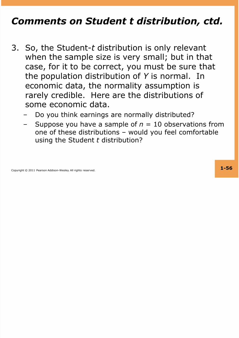
Comments on Student t distribution, ctd.
3.
So, the Student-t distribution is only relevantwhen the sample size is very small; but in thatcase, for it to be correct, you must be sure thatthe population distribution of Y is normal. In
economic data, the normality assumption israrely credible. Here are the distributions ofsome economic data.
– Do you think earnings are normally distributed?
–
Suppose you have a sample of n = 10 observations fromone of these distributions – would you feel comfortableusing the Student t distribution?
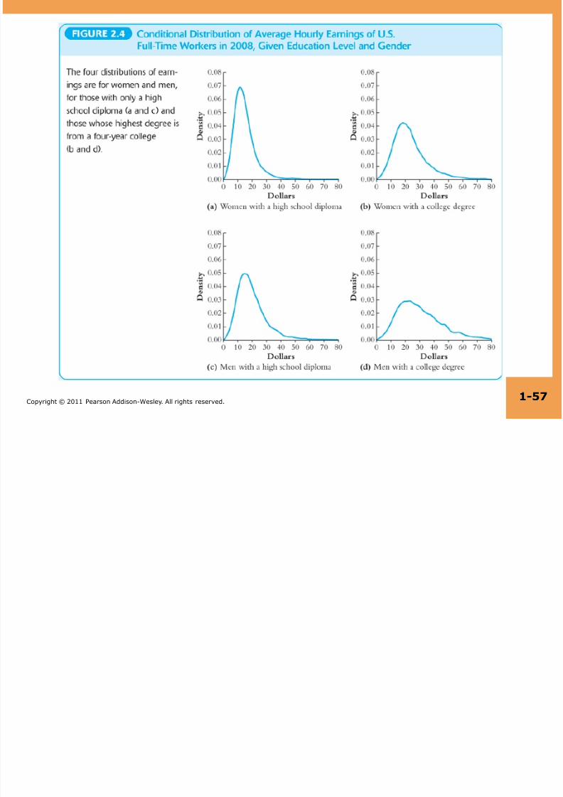
7/21/2019 ECON 491: ECONOMETRICS STOCK AND WATSON PPT
http://slidepdf.com/reader/full/econ-491-econometrics-stock-and-watson-ppt 57/63
Copyright © 2011 Pearson Addison-Wesley. All rights reserved. 1-57

7/21/2019 ECON 491: ECONOMETRICS STOCK AND WATSON PPT
http://slidepdf.com/reader/full/econ-491-econometrics-stock-and-watson-ppt 58/63
Copyright © 2011 Pearson Addison-Wesley. All rights reserved. 1-58
Comments on Student t distribution, ctd.
4.
You might not know this. Consider the t -statistic testingthe hypothesis that two means (groups s, l ) are equal:
Even if the population distribution of Y in the two groups isnormal, this statistic doesn’t have a Student t distribution!
There is a statistic testing this hypothesis that has a normaldistribution, the pooled variance” t -statistic – see SW
(Section 3.6) – however the pooled variance t -statistic isonly valid if the variances of the normal distributions arethe same in the two groups. Would you expect this to betrue, say, for men’s v. women’s wages?
t =Y s !Y
l
s s
2
n s
+ sl
2
nl
=
Y s !Y
l
SE (Y s !Y
l )

7/21/2019 ECON 491: ECONOMETRICS STOCK AND WATSON PPT
http://slidepdf.com/reader/full/econ-491-econometrics-stock-and-watson-ppt 59/63
Copyright © 2011 Pearson Addison-Wesley. All rights reserved. 1-59
The Student-t distribution – Summary
•
The assumption that Y is distributed N (! Y , ) is rarely plausiblein practice (Income? Number of children?)
• For n > 30, the t -distribution and N (0,1) are very close (as n grows large, the t n–1 distribution converges to N (0,1))
• The t -distribution is an artifact from days when sample sizes weresmall and computers” were people
• For historical reasons, statistical software typically uses the t -distribution to compute p-values – but this is irrelevant when thesample size is moderate or large.
• For these reasons, in this class we will focus on the large-n approximation given by the CLT
1.
The probability framework for statistical inference2. Estimation
3.
Testing
4. Confidence intervals
! Y
2

7/21/2019 ECON 491: ECONOMETRICS STOCK AND WATSON PPT
http://slidepdf.com/reader/full/econ-491-econometrics-stock-and-watson-ppt 60/63
Copyright © 2011 Pearson Addison-Wesley. All rights reserved. 1-60
Confidence Intervals
•
A 95% confidence interval for ! Y is an intervalthat contains the true value of ! Y in 95% ofrepeated samples.
• Digression: What is random here? The values of
Y 1,...,Y n and thus any functions of them –including the confidence interval. The confidenceinterval will differ from one sample to the next.The population parameter, ! Y , is not random; we
just don’t know it.

7/21/2019 ECON 491: ECONOMETRICS STOCK AND WATSON PPT
http://slidepdf.com/reader/full/econ-491-econometrics-stock-and-watson-ppt 61/63
Copyright © 2011 Pearson Addison-Wesley. All rights reserved. 1-61
Confidence intervals, ctd.
A 95% confidence interval can always be constructed as the setof values of ! Y not rejected by a hypothesis test with a 5%significance level.
{! Y : $ 1.96} = {! Y : –1.96 $ $ 1.96}
= {! Y : –1.96 $ – ! Y $ 1.96 }
= {! Y # ( – 1.96 , + 1.96 )}
This confidence interval relies on the large-n results that is
approximately normally distributed and .
Y ! µ Y
sY / n
Y ! µ Y
sY / n
sY
n
sY
n
sY
nY
Y
sY
2
!
p
!
Y
2
Y

7/21/2019 ECON 491: ECONOMETRICS STOCK AND WATSON PPT
http://slidepdf.com/reader/full/econ-491-econometrics-stock-and-watson-ppt 62/63
Copyright © 2011 Pearson Addison-Wesley. All rights reserved. 1-62
Summary:
From the two assumptions of:1.
simple random sampling of a population, that is,
{Y i , i =1,…,n} are i.i.d.
2. 0 < E (Y 4) < #
we developed, for large samples (large n):–
Theory of estimation (sampling distribution of )
–
Theory of hypothesis testing (large-n distribution of t -statistic and computation of the p-value)
–
Theory of confidence intervals (constructed by invertingthe test statistic)
Are assumptions (1) & (2) plausible in practice? Yes
Y
L t b k t th i i l li

7/21/2019 ECON 491: ECONOMETRICS STOCK AND WATSON PPT
http://slidepdf.com/reader/full/econ-491-econometrics-stock-and-watson-ppt 63/63
Let
s go back to the original policyquestion:
What is the effect on test scores of reducing STR by onestudent/class?
Have we answered this question?