1/24

ECON 4624 – Income taxation

2/24

Why is it important?

An important source of revenue in most countries (60 - 70%)

Affect labour and capital (savings) supply and overall economicactivity – how much depend on the elasticity of labour (capital)supply.

Creates an efficiency loss - a dead weight loss - magnitude dependon the compensated supply elasticity

Tax reforms can be used to estimate how labour supply responds towage changes – important topic.

3/24

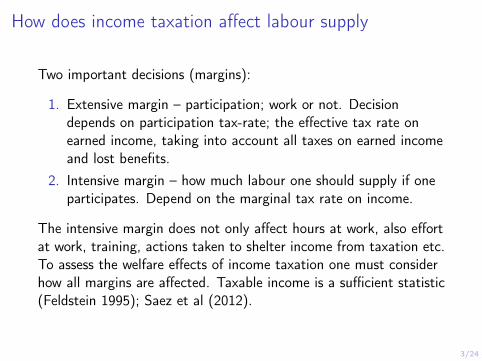
How does income taxation affect labour supply

Two important decisions (margins):

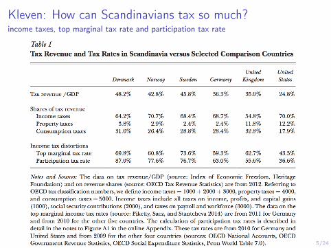
1. Extensive margin – participation; work or not. Decisiondepends on participation tax-rate; the effective tax rate onearned income, taking into account all taxes on earned incomeand lost benefits.

2. Intensive margin – how much labour one should supply if oneparticipates. Depend on the marginal tax rate on income.

The intensive margin does not only affect hours at work, also effortat work, training, actions taken to shelter income from taxation etc.To assess the welfare effects of income taxation one must considerhow all margins are affected. Taxable income is a sufficient statistic(Feldstein 1995); Saez et al (2012).

4/24

Kleven: How can Scandinavians tax so much?

The same question that funded ESOP: Based on economic theory itis (is it?) a paradox that Scandinavian work and produce so much.

Kleven discusses three explanations.

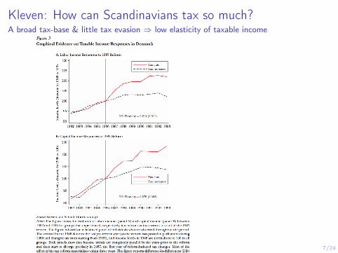
1. Little tax evasion and a broad tax base implies a low elasticityof taxable income.

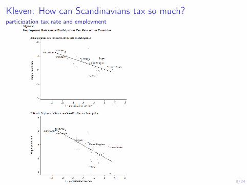
2. Scandinavian countries counters the effect of high participationtax rate by subsidizing services that are complementary towork (child care, old age care , education ..)

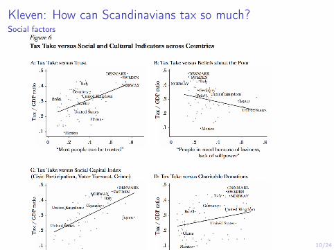
3. Social cultural factors. Trust in people, and in government etc.

5/24

Kleven: How can Scandinavians tax so much?income taxes, top marginal tax rate and participation tax rate

6/24

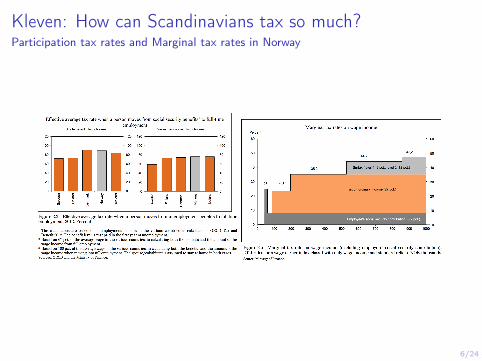
Kleven: How can Scandinavians tax so much?Participation tax rates and Marginal tax rates in Norway

7/24

Kleven: How can Scandinavians tax so much?A broad tax-base & little tax evasion ) low elasticity of taxable income

8/24

Kleven: How can Scandinavians tax so much?participation tax rate and employment

9/24

Kleven: How can Scandinavians tax so much?work subsidies

10/24

Kleven: How can Scandinavians tax so much?Social factors

11/24

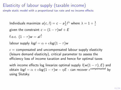
Elasticity of labour supply (taxable income)simple static model with a proportional tax rate and no income effects

Individuals maximize u(c, l) = c � a

1� l

� where � = 1 + 1✏

given the constraint c = (1 � ⌧)wl + E

f.o.c. (1 � ⌧)w = al

1✏

labour supply logl = ↵+ ✏log(1 � ⌧)w

✏ = compensated and uncompensated labour supply elasticity(leisure demand elasticity), critical parameter to assess theefficiency loss of income taxation and hence for optimal taxes

with income effects log linearize optimal supply l(w(1 � ⌧),E ) andobtain logl = ↵+ ✏log(1 � ⌧)w � ⌘E - can recover ✏compensated byusing Slutsky.

12/24

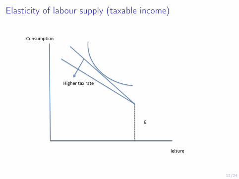
Elasticity of labour supply (taxable income)

leisure'

Consump-on''

E'

Higher'tax'rate'

13/24

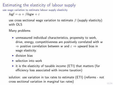
Estimating the elasticity of labour supplyuse wage variation to estimate labour supply elasticity

logl = ↵+ �logw + "

use cross sectional wage variation to estimate � (supply elasticity)with OLS

Many problems

I unmeasured individual characteristics, propensity to work,drive, energy, competitiveness are positively correlated with w

) positive correlation between w and " ) upward bias inwage elasticity.

I division biasI selection into workI it is the elasticity of taxable income (ETI) that matters (for

efficiency loss associated with income taxation)

solution: use variation in tax rates to estimate (ETI) (reforms - notcross sectional variation in marginal tax rates)

14/24

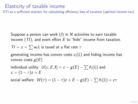
Elasticity of taxable incomeETI as a sufficient statistic for calculating efficiency loss of taxation (optimal income tax).

Suppose a person can work (l) in N activities to earn taxableincome (TI ), and exert effort E to “hide” income from taxation.

TI = z =P

w

i

l

i

is taxed at a flat rate ⌧

generating income has convex costs c

i

(li

) and hiding income hasconvex costs g(E )

individual utility: U(c,E , l) = c � g(E )�P

✓i

(li

) andc = (1 � ⌧)z + E

social welfare: W (⌧) = (1 � ⌧)z + E � g(E )�P

✓i

(li

) + z⌧

15/24

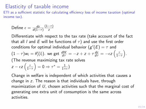
Elasticity of taxable incomeETI as a sufficient statistic for calculating efficiency loss of income taxation (optimal

income tax).

Define ✏ = dz

d(1�⌧)(1�⌧)

z

Differentiate with respect to the tax rate (take account of the factthat all l and E will be functions of ⌧) and use the first orderconditions for optimal individual behavior (g 0(E ) = ⌧ and(1 � ⌧)w

i

= ✓0i

(li

). we get dW

d⌧ = �z + z + ⌧ dz

d⌧ = �✏z⇣

⌧1�⌧

⌘.

(The revenue maximizing tax rate solvesz � ✏z

⇣⌧

1�⌧

⌘= 0 ) ⌧⇤ = 1

1+✏)

Change in welfare is independent of which activities that causes achange in z . The reason is that individuals have, throughmaximization of U, chosen activities such that the marginal cost ofgenerating one extra unit of consumption is the same acrossactivities.

16/24

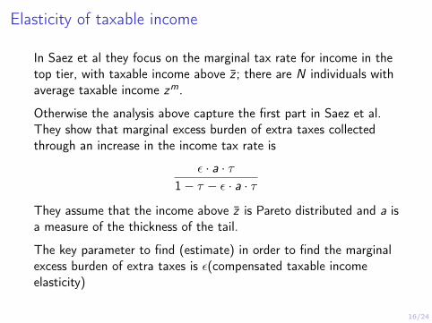
Elasticity of taxable income

In Saez et al they focus on the marginal tax rate for income in thetop tier, with taxable income above z̄ ; there are N individuals withaverage taxable income z

m.

Otherwise the analysis above capture the first part in Saez et al.They show that marginal excess burden of extra taxes collectedthrough an increase in the income tax rate is

✏ · a · ⌧1 � ⌧ � ✏ · a · ⌧

They assume that the income above z̄ is Pareto distributed and a isa measure of the thickness of the tail.

The key parameter to find (estimate) in order to find the marginalexcess burden of extra taxes is ✏(compensated taxable incomeelasticity)

17/24

Elasticity of taxable income

Complications (reasons why the elasticity of taxable (reported)income is not a sufficient statistic for welfare analysis)

I Externalities (activities to hide income may have positive ornegative effects on other sources of government revenue (or onother individuals).

I Log term responsesI ..

18/24

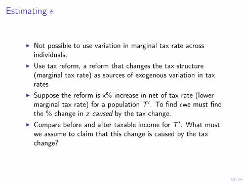
Estimating ✏

I Not possible to use variation in marginal tax rate acrossindividuals.

I Use tax reform, a reform that changes the tax structure(marginal tax rate) as sources of exogenous variation in taxrates

I Suppose the reform is x% increase in net of tax rate (lowermarginal tax rate) for a population T

0. To find ✏we must findthe % change in z caused by the tax change.

I Compare before and after taxable income for T

0. What mustwe assume to claim that this change is caused by the taxchange?

19/24

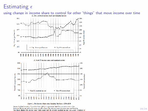
Estimating ✏using change in income share to control for other “things” that move income over time

20/24

Estimating ✏

I Compare before and after taxable income for T

0 withindividuals who where not treated with an increase in the netof tax rate, or who was less treated. DiD.

I Many papers that exploit such reforms - elasticity estimatesvaries from far above 1 to close to 0. Some of these estimatesindicate that one is on the wrong side of the laffer curve.

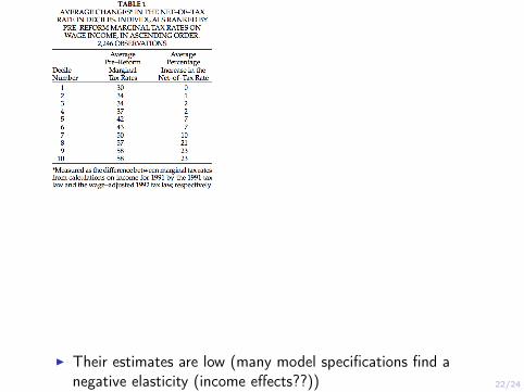
I A paper by Thoresen and Aarby (2001) uses the 1992 taxreform to estimate ".

21/24

Estimating "

22/24

I Their estimates are low (many model specifications find anegative elasticity (income effects??))

22/24

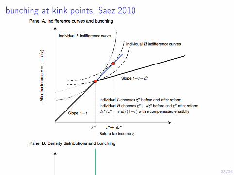
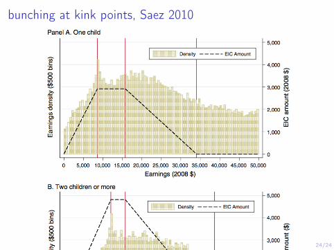
bunching at kink points, Saez 2010

The idea is that one can use sharp increases in the marginal taxrate at certain points to estimate compensated elasticities bymeasuring the magnitude of bunching observed at the kink pointsin the budget set.

Saez finds modest effects (not much bunching); largest effect forlow income.

23/24

bunching at kink points, Saez 2010

24/24

bunching at kink points, Saez 2010