Embed Size (px)
Citation preview
ECON 459 — Game Theory
Lecture Notes
Nash Bargaining
Luca Anderlini — Spring 2017
These notes have been used and commented on before. If you can still spotany errors or have any suggestions for improvement, please let me know.
1 Bargaining Theory – Pream-ble
• Economic transactions generate surplus.
• Bargaining Theory addresses the question of how the
surplus will be divided among the participants.
• In virtually all cases it is restricted to the case of two
agents.
• Suppose one agent has an object to sell, and another h
as the opportunity to buy it.
• Suppose the seller values the object less than the po-
tential buyer. The difference between the valuation of
the seller and that of the buyer is the potential surplus.
• Since there are mutual gains from trade, it is reasonable
to suppose that the transaction will take place.
• The objective of Bargaining Theory is to say something
(if possible to pin down completely) about the price at
which the transaction will take place.
• Another way to put it is that Bargaining Theory ad-
dresses the question: How will the surplus be split
between the two?
• Once we frame the question in terms of surplus, we
have a framework that applies much more generally than
1
the single-object transaction. The two agents could, for
instance, be bargaining over the terms of a complex con-
tractual arrangement.
• Lastly, notice that price-taking models are no use what-
soever in answering the question at hand.
• Bargaining Theory studies situation in which no-one
can reasonably be assumed to be taking the price as given.
•The question in Bargaining Theory is precisely: Where
do the prices come from in a situation of bilateral
monopoly?
• Two types of Bargaining Theory have been developed.
• The first one we look at is also the first one to have been
developed historically. It is known as “Nash Bargaining.”
• This way of proceeding amounts to stating a number
of “desirable properties” that the “solution” to a bar-
gaining problem should have, and then showing that the
properties in fact do pin down the solution uniquely.
• Nash Bargaining belongs to a body of work called “Co-
operative Game Theory.”
• The second approach to Bargaining Theory belongs
firmly to Non-Cooperative Game Theory (the stuff we
have been concerned with so far).
2
• In this approach, we write down an extensive form game
that we think captures the essence of how the bargaining
will in fact proceed. We then apply the tools of Non-
Cooperative Game Theory to solve the extensive form
game and – hopefully – find a unique prediction about
the outcome.
• One of the surprises we find along the way is that the
solutions to the bargaining problem we find using these
two – seemingly unrelated – approaches are in fact closely
related. Under appropriate circumstances the answer is
the same.
2 Nash Bargaining
2.1 Ingredients: The Set-Up
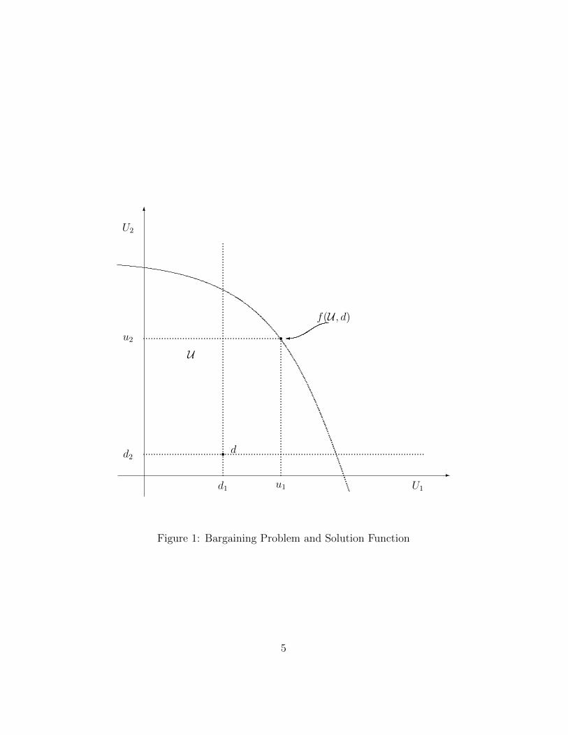
• There are two participants, i = 1, 2.
• A bargaining problem is a pair B = (U , d).
• In (U , d), U is a set of possible agreements in terms
of utilities that they yield to 1 and 2. An element of Uis a pair u = (u1, u2) ∈ U .
• The interpretation is that if agreement u = (u1, u2) ∈U is reached, then 1 gets utility u1 and 2 gets utility u2.
3
• Throughout, we are going to take U to be a convex set.
• In (U , d), d is a pair (d1, d2) called the disagreement
point.
• The interpretation is that if no agreement is reached
then 1 gets utility d1 and 2 gets utility d2.
2.2 Ingredients: The SolutionFunction
• What sort of “solution” are we after?
• We seek a “solution function” f of the following kind.
• The function f takes as input any bargaining problem
(U , d), and returns a pair of utilities u = (u1, u2) ∈ U .
• So, we write u = f (B) or alternatively u = f (U , d).
When we need to refer to the “components” of f we write
u1 = f1(B) and u2 = f2(B) or alternatively u1 = f1(U , d)
and u2 = f2(U , d).
• The interpretation is that, given any bargaining
problem B = (U , d), the solution function tells us that
the agreement u = f (U , d) will be reached.
4
6
-
r........................................
U1
U2
d
d1
d2
U
f(U , d)�r
...
...
...
...
...
...
...
...
...
...
...
...
...
...
...
...
...
...
...
...
...
...
...
...
...
...
...
.............................................................................
.....................................................
.....................................................
u1
u2
Figure 1: Bargaining Problem and Solution Function
5
2.3 A Canonical Interpretation
• There are a buyer and a seller.
• The seller has an object potentially for sale that costs
him c.
• The buyer places a value of v on the object.
• To make this interesting we take it to be the case that
v > c.
• At what price p will the object be sold?
• If it is sold at p, then the seller’s utility is US(p − c)and the buyer’s utility is UB(v − p).
• If no transaction takes place, then both buyer and seller
get a utility of 0.
• This situation gives rise to a bargaining problem of the
type we described in the abstract before.
• Take U to be the set of utility pairs that can be obtained
as p varies between c and v. (So, notice if both UB and
US are concave, we get a convex U .)
• Take d to be (0, 0).
• A Solution function would tell us what utility the buyer
and the seller get, and hence the price at which the object
is traded.
6
2.4 Question
• Suppose we list a bunch of “appealing” properties that
f should satisfy.
• Can we “pin down” f completely?
• Answer: YES.
2.5 The Axioms
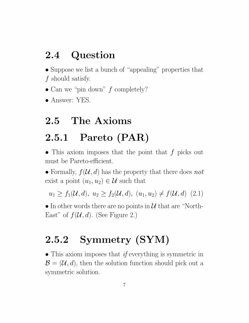
2.5.1 Pareto (PAR)
• This axiom imposes that the point that f picks out
must be Pareto-efficient.
• Formally, f (U , d) has the property that there does not
exist a point (u1, u2) ∈ U such that
u1 ≥ f1(U , d), u2 ≥ f2(U , d), (u1, u2) 6= f (U , d) (2.1)
• In other words there are no points in U that are “North-
East” of f (U , d). (See Figure 2.)
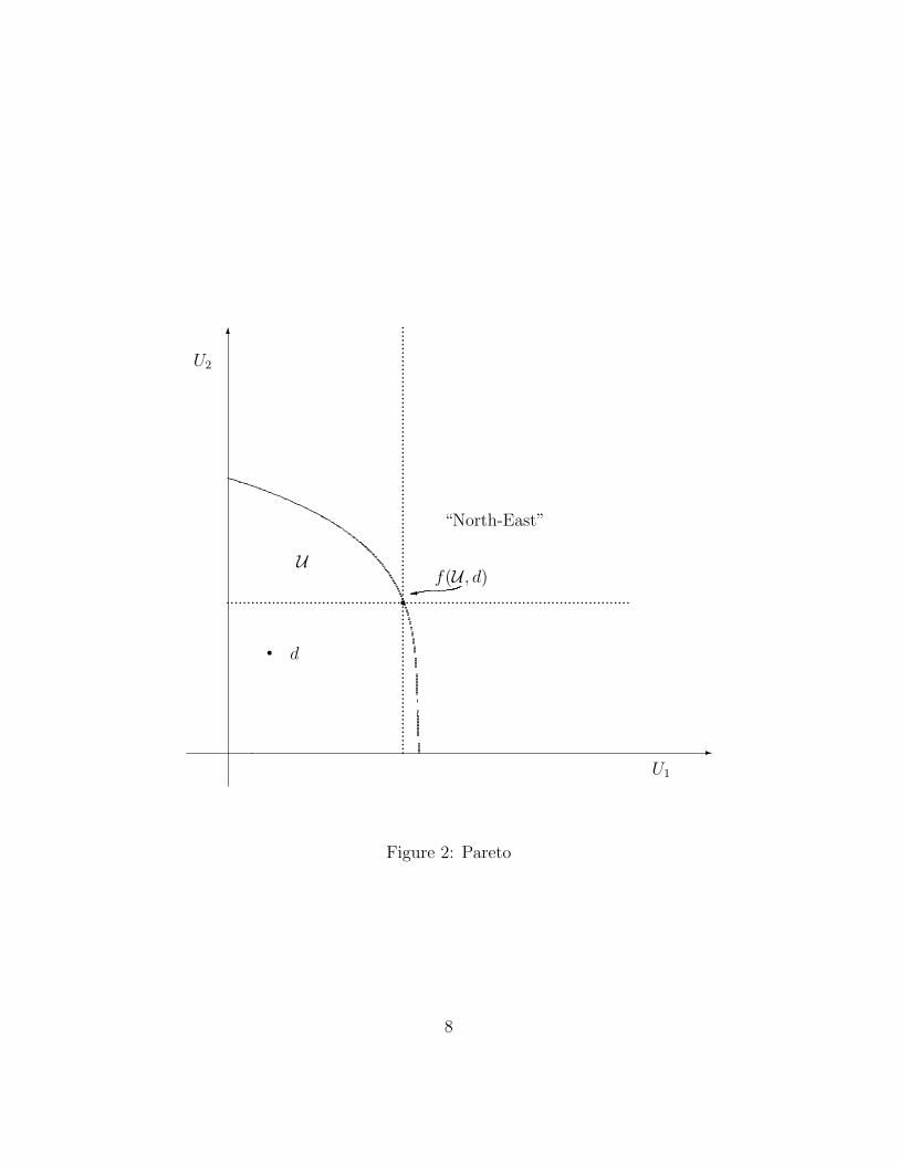
2.5.2 Symmetry (SYM)
• This axiom imposes that if everything is symmetric in
B = (U , d), then the solution function should pick out a
symmetric solution.
7
6
-
U1
U2
rr
...
...
...
...
...
...
...
...
...
...
...
...
...
...
...
...
...
...
...
...
...
...
...
...
...
...
...
...
...
...
...
...
...
...
.
.................................................................................................
d
f(U , d)�
U
“North-East”
Figure 2: Pareto
8
6
-
U1
U2
................................................................................................................
45o
rd
r f(U , d)�
Figure 3: Symmetry
• Formally, suppose that (U , d) is such that U is sym-
metric around the 45o line and d1 = d2, then
f1(U , d) = f2(U , d) (2.2)
• In other words, when everything in B is symmetric, the
point f (U , d) is itself on the 45o line. (See Figure 3.)
9
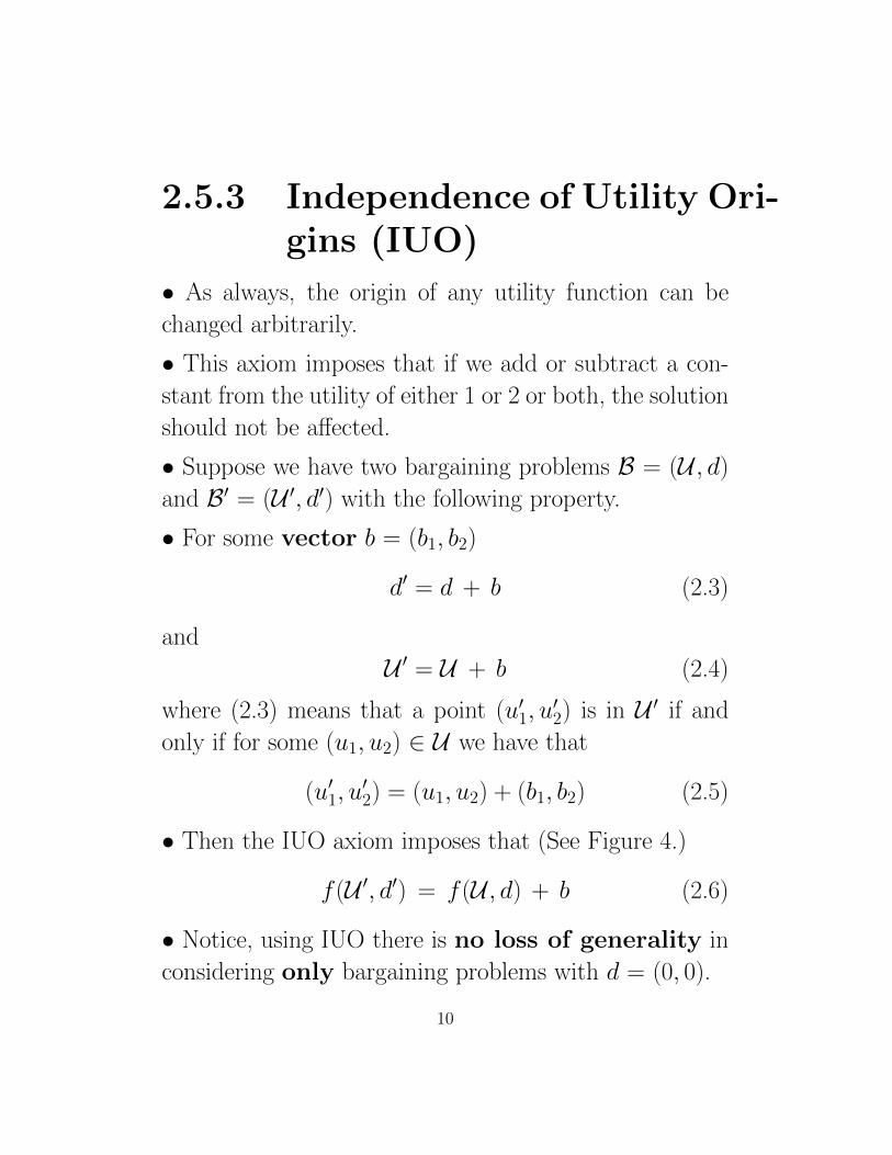
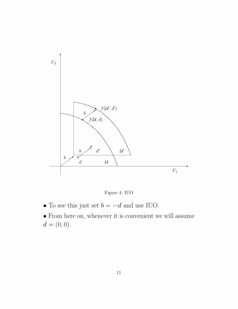
2.5.3 Independence of Utility Ori-gins (IUO)
• As always, the origin of any utility function can be
changed arbitrarily.
• This axiom imposes that if we add or subtract a con-
stant from the utility of either 1 or 2 or both, the solution
should not be affected.
• Suppose we have two bargaining problems B = (U , d)
and B′ = (U ′, d′) with the following property.
• For some vector b = (b1, b2)
d′ = d + b (2.3)
and
U ′ = U + b (2.4)
where (2.3) means that a point (u′1, u′2) is in U ′ if and
only if for some (u1, u2) ∈ U we have that
(u′1, u′2) = (u1, u2) + (b1, b2) (2.5)
• Then the IUO axiom imposes that (See Figure 4.)
f (U ′, d′) = f (U , d) + b (2.6)
• Notice, using IUO there is no loss of generality in
considering only bargaining problems with d = (0, 0).
10
6
-
U1
U2
rd
rd′
......................................................................................................
rr
U
U ′
f(U , d)
f(U ′, d′)
����>
����>
����>b
b
b
Figure 4: IUO
• To see this just set b = −d and use IUO.
• From here on, whenever it is convenient we will assume
d = (0, 0).
11
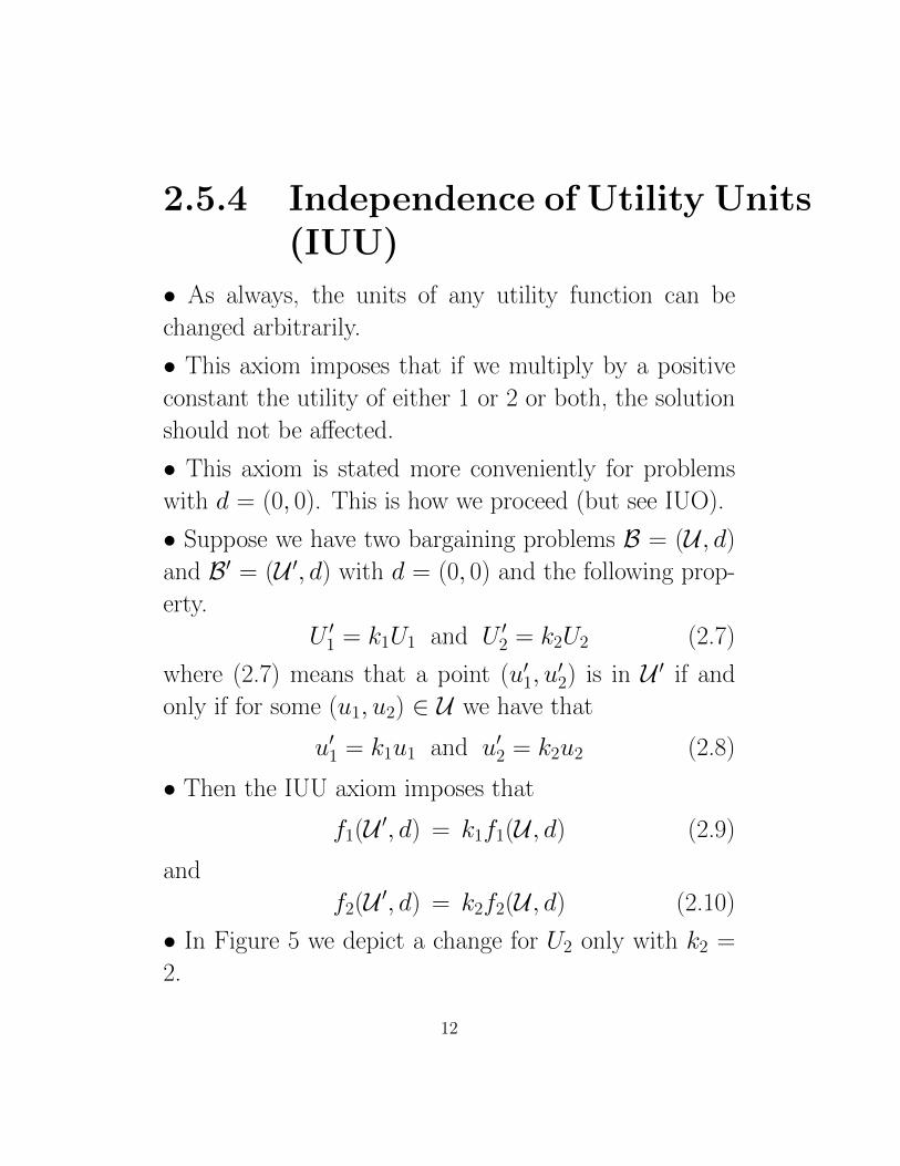
2.5.4 Independence of Utility Units(IUU)
• As always, the units of any utility function can be
changed arbitrarily.
• This axiom imposes that if we multiply by a positive
constant the utility of either 1 or 2 or both, the solution
should not be affected.
• This axiom is stated more conveniently for problems
with d = (0, 0). This is how we proceed (but see IUO).
• Suppose we have two bargaining problems B = (U , d)
and B′ = (U ′, d) with d = (0, 0) and the following prop-
erty.
U ′1 = k1U1 and U ′2 = k2U2 (2.7)
where (2.7) means that a point (u′1, u′2) is in U ′ if and
only if for some (u1, u2) ∈ U we have that
u′1 = k1u1 and u′2 = k2u2 (2.8)
• Then the IUU axiom imposes that
f1(U ′, d) = k1f1(U , d) (2.9)
and
f2(U ′, d) = k2f2(U , d) (2.10)
• In Figure 5 we depict a change for U2 only with k2 =
2.
12
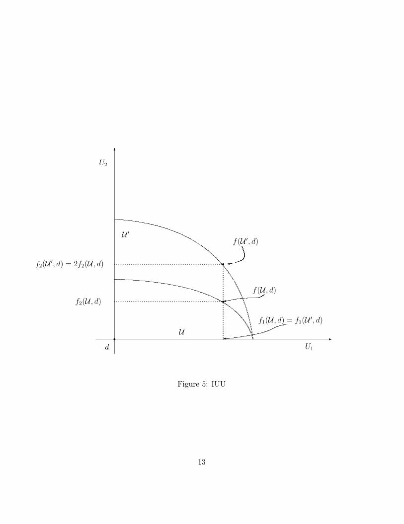
6
-
U1
U2
U
U ′
p
r.........................................
...........................................................
...........................................................
d
r
rf1(U , d) = f1(U ′, d)
�
f(U , d)�
f(U ′, d)
�f2(U ′, d) = 2f2(U , d)
f2(U , d)
Figure 5: IUU
13
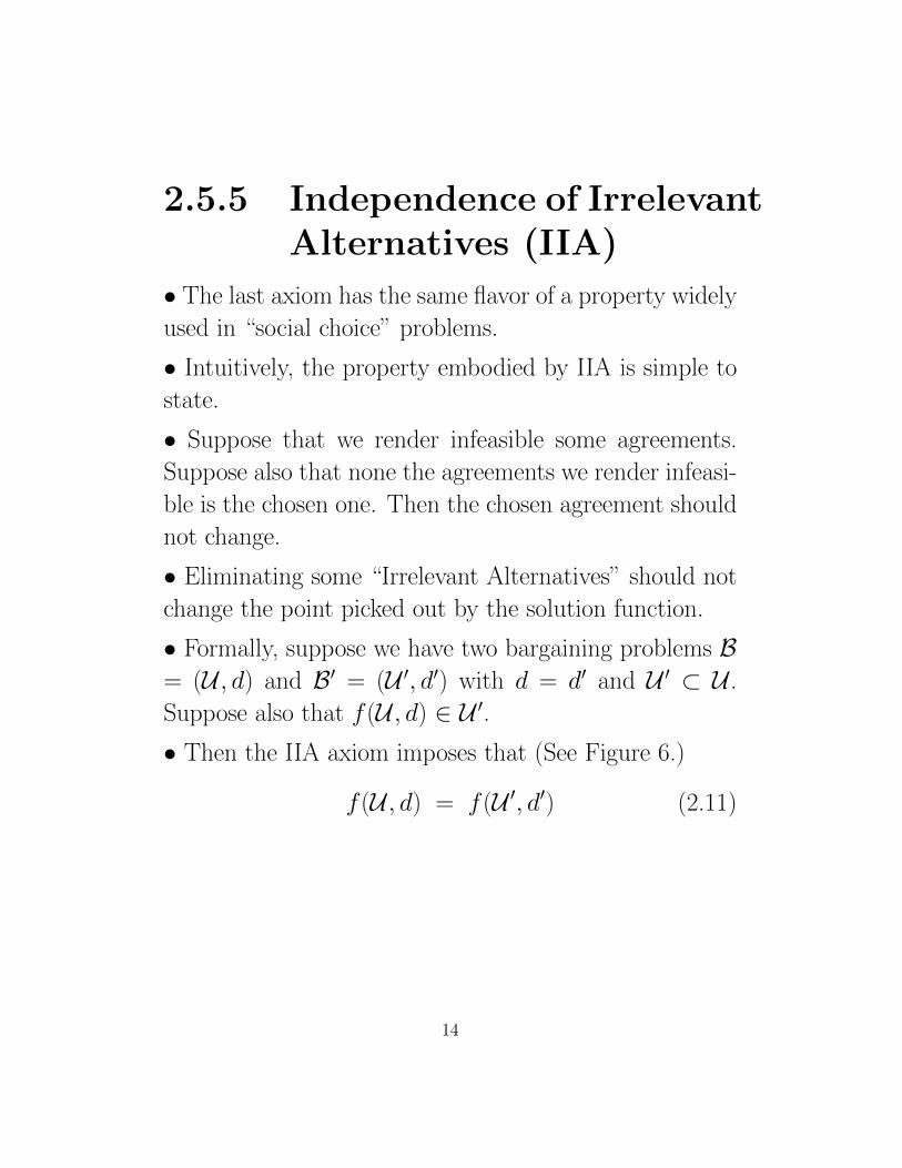
2.5.5 Independence of IrrelevantAlternatives (IIA)
• The last axiom has the same flavor of a property widely
used in “social choice” problems.
• Intuitively, the property embodied by IIA is simple to
state.
• Suppose that we render infeasible some agreements.
Suppose also that none the agreements we render infeasi-
ble is the chosen one. Then the chosen agreement should
not change.
• Eliminating some “Irrelevant Alternatives” should not
change the point picked out by the solution function.
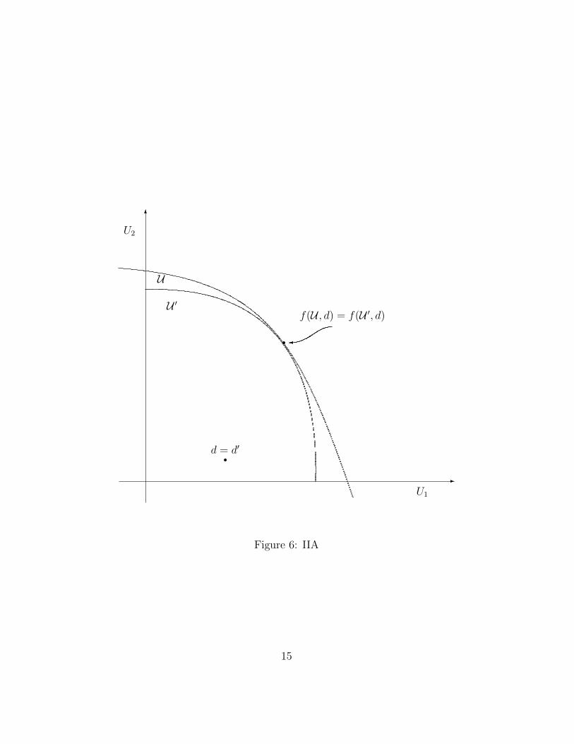
• Formally, suppose we have two bargaining problems B= (U , d) and B′ = (U ′, d′) with d = d′ and U ′ ⊂ U .
Suppose also that f (U , d) ∈ U ′.• Then the IIA axiom imposes that (See Figure 6.)
f (U , d) = f (U ′, d′) (2.11)
14
6
-
rU1
U2
d = d′
f(U , d) = f(U ′, d)
�rU ′
U
Figure 6: IIA
15
2.6 Pinning Down f
2.6.1 Symmetric Problems
• Our first observation is that because of PAR and SYM,
we know everything about f (B) = f (U , d) if B ia sym-
metric problem (d1 = d2 and U symmetric around the
45o line).
• In this case f (U , d) must be on the upper boundary of
U on the 45o line.
• These two requirements together pin down f uniquely,
just as in Figure 3.
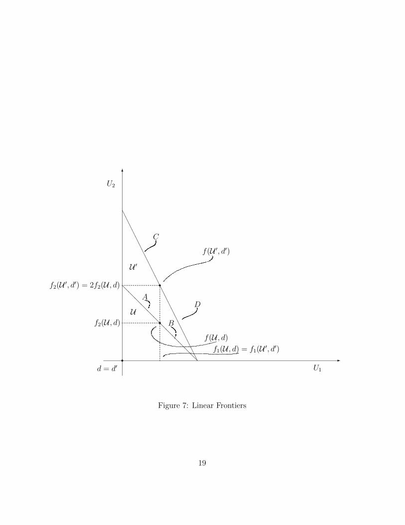
2.6.2 Linear Frontier Problems
• Our second observation concerns any B with a linear
frontier.
•We say that a bargaining problem B has a linear frontier
if and only if the upper boundary of U is a (downward
sloping) straight line.
• To argue what f has to be like in the case of a linear
frontier B we proceed in two steps.
•We do this setting d1 = d2 = 0 for simplicity. (We know
this can always be done.)
16
• From our observation about symmetric problems above,
we know that if B has a linear frontier and is also sym-
metric, then
f1(U , d) = f2(U , d) (2.12)
• Now consider a symmetric B with a linear frontier and
notice that in this case the slope of the upper boundary
of U must be −1.
• It follows that the segment (up) on the left of f (U , d)
on the frontier of U must be of the same length as the
segment (down) on the right of f (U , d) on the frontier of
U . (See Figure 7 – the two segments A and B have the
same length.)
• Now consider a new linear frontier bargaining problem
B′ = (U ′, d′) with d′ = d, and U ′ with a boundary that
cuts the horizontal axis in the same place as U , but cuts
the vertical axis twice as high as U . (See Figure 7.)
• Notice B′ is not a symmetric problem.
• However, IUU tells us what the solution f (U ′, d′ should
be.
• Since we have kept U1 the same and we have multiplied
U2 by 2 (see Figure 7), we should have
f1(U ′, d′) = f1(U , d) (2.13)
17
and
f2(U ′, d′) = 2 f2(U , d) (2.14)
• But this (see Figure 7) tells us something general
about bargaining problems with a linear frontier — sym-
metric or not.
• Geometrically, in Figure 7, it is clear that the triangle
above the dotted line has the same shape and dimensions
as the triangle to the right of the dotted line.
• Hence, it follows that in Figure 7 the segment (up) on
the left of f (U ′, d′) on the frontier of U ′ must be of the
same length as the segment (down) on the right of
f (U ′, d′) on the frontier of U ′ — the two segments C and
D have the same length.
• We have done this diagrammatically scaling U2 by a
factor of 2. But clearly the geometric argument gener-
alizes to any re-scaling of a symmetric problem with a
linear frontier.
• Hence, we have reached the following key conclusion.
• In any bargaining problem B = (U , d) with d = (0, 0)
and with a linear frontier (whether symmetric or not),
f (U , d) picks out the point on the frontier of U that di-
vides the frontier into two segments of equal length.
18
6
-
U1
U2
@@@@@@@@@@@@
d = d′r ...
...
...
...
...
...
........................r
r
AAAAAAAAAAAAAAAAAAAAAAA
..........................................U
U ′
A
Bf2(U , d)
f(U , d)
f(U ′, d′)
C
D
f1(U , d) = f1(U ′, d′)
f2(U ′, d′) = 2f2(U , d)
Figure 7: Linear Frontiers
19
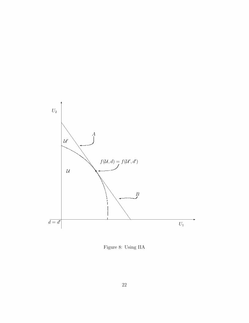
2.6.3 Using IIA
• We now know everything there is to know about bar-
gaining problems with a linear frontier.
• Using IIA, this will be enough to pin down f in the
general case.
• Start with any bargaining problem B = (U , d), not
necessarily with a linear frontier and not necessarily sym-
metric.
• For the time being assume that d1 = d2 = 0. We will
come back to this shortly.
• Now find the tangent to the frontier that also has the
property that the segment (up) on the left of the tangency
point is of the same length as the segment (down) on
the right of the tangency point. (See figure 8 – the two
segments A and B have the same length.)
• Doing this we have constructed a new bargaining prob-
lem B′ = (U ′, d′) with d′ = d, and with U ′ the area below
the tangent. (See figure 8.)
• Clearly, the bargaining problem B′ = (U ′, d′) has a
linear frontier. We constructed it this way! We also have
d′ = 0.
• Hence, we know everything about f (U ′, d′).
20
• In particular, the solution f (U ′, d′) must be as in Figure
8.
• Now we are ready to use IIA.
• Going from B′ = (U ′, d′) to B = (U , d) we shrink the
feasible set from U ′ to U , we do not change the disagree-
ment point, and we do not take out the solution to B′.• Hence IIA tells us that, as in Figure 8, we must have
that
f (U , d) = f (U ′, d′) (2.15)
• To summarize, so far we know the following.
• Consider any B = (U , d) with d = (0, 0).
• Then to find f (U , d) we can proceed as follows.
• Find the point on the frontier of U that has the following
property.
• When we draw the tangent to U at this point, the
length of the two segments on the tangent, from the
tangency point to the vertical axis, and from the tangency
point to the horizontal axis is the same. (See figure 8
— the length of A and B is the same.)
2.6.4 Using IUO (Again)
•We know how to find f (U , d), provided that d = (0, 0).
21
6
-
U1
U2
SSSSSSSSSSSSSSSSSSSSSSSS
r
d = d′
U
U ′
f(U , d) = f(U ′, d′)
�
A
B
�
�
Figure 8: Using IIA
22
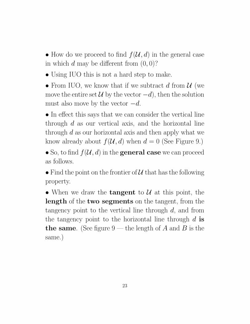
• How do we proceed to find f (U , d) in the general case
in which d may be different from (0, 0)?
• Using IUO this is not a hard step to make.
• From IUO, we know that if we subtract d from U (we
move the entire set U by the vector−d), then the solution
must also move by the vector −d.
• In effect this says that we can consider the vertical line
through d as our vertical axis, and the horizontal line
through d as our horizontal axis and then apply what we
know already about f (U , d) when d = 0 (See Figure 9.)
• So, to find f (U , d) in the general case we can proceed
as follows.
• Find the point on the frontier of U that has the following
property.
• When we draw the tangent to U at this point, the
length of the two segments on the tangent, from the
tangency point to the vertical line through d, and from
the tangency point to the horizontal line through d is
the same. (See figure 9 — the length of A and B is the
same.)
23
6
-
U1
U2
rd
.....................................................................................................
...................................................................................................................
ZZZZZZZZZZZZZZZZZZZZZZZZZ
rU f(U , d)..............................................................................................
f1(U , d)
f2(U , d)
A
B
�
?
Figure 9: Using IUO Again
24
2.7 Finding f in Practice
• Our analysis so far shows that for any B = (U , d),
f (U , d) is pinned down uniquely by PAR, SYM, IUO,
IUU and IIA.
• Geometrically, we also now know how to find f (U , d)
in the general case.
• This is exemplified in Figure 9.
•We seek a way to find the solution using a mathematical
method.
• To do this, begin with some facts concerning hyperbo-
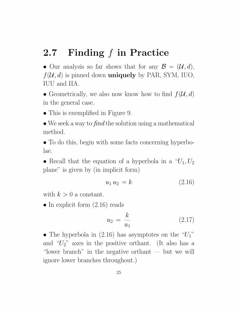
lae.
• Recall that the equation of a hyperbola in a “U1, U2
plane” is given by (in implicit form)
u1 u2 = k (2.16)
with k > 0 a constant.
• In explicit form (2.16) reads
u2 =k
u1(2.17)
• The hyperbola in (2.16) has asymptotes on the “U1”
and “U2” axes in the positive orthant. (It also has a
“lower branch” in the negative orthant — but we will
ignore lower branches throughout.)
25
• If we want to write the (implicit) equation of a hy-
perbola with a vertical asymptote at v and a horizontal
asymptote at h we need to subtract these as constants
from u1 and u2 respectively.
• So we get
(u1 − v) (u2 − h) = k (2.18)
with k > 0 a constant.
• Notice that as we increase k in (2.18) we describe a
family of hyperbolae which move in the “North-East”
direction as k increases. (With given asymptotes if we
keep v and h constant.)
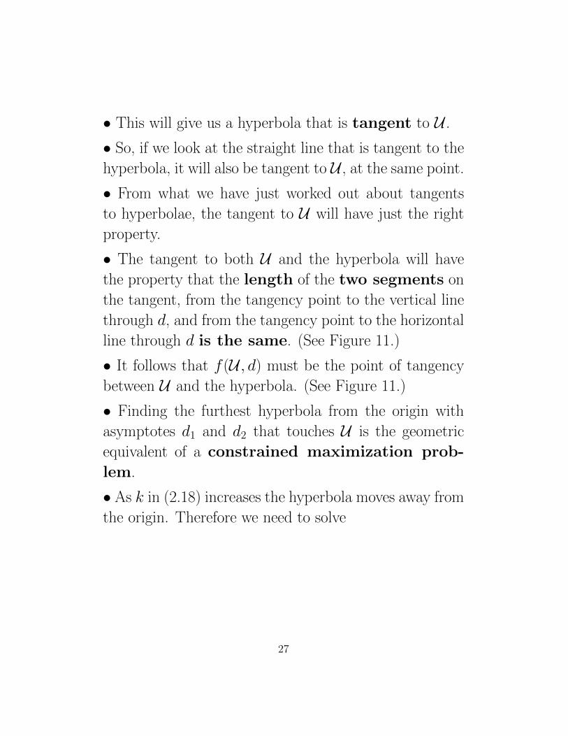
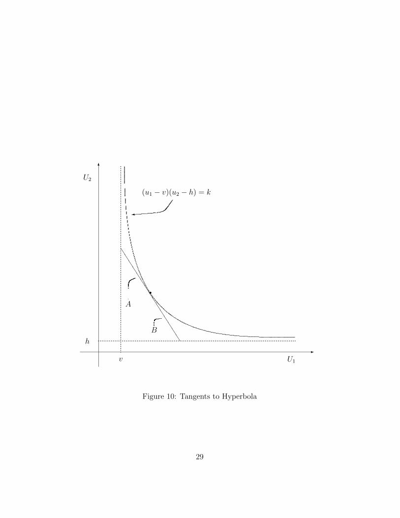
• An important fact about these hyperbolae is the fol-
lowing.
• If we draw the tangent to the hyperbola in (2.18) at
any point, the length of the two segments on the
tangent, from the tangency point to the vertical asymp-
tote, and from the tangency point to the horizontal asymp-
tote is the same. (See figure 10 — the length of A and
B is the same.)
• This fact suggests the following method for finding
f (U , d) for a general bargaining problem.
• We should find the furthest hyperbola from the origin
(going “North-East”) with asymptotes d1 and d2 that
touches U .
26
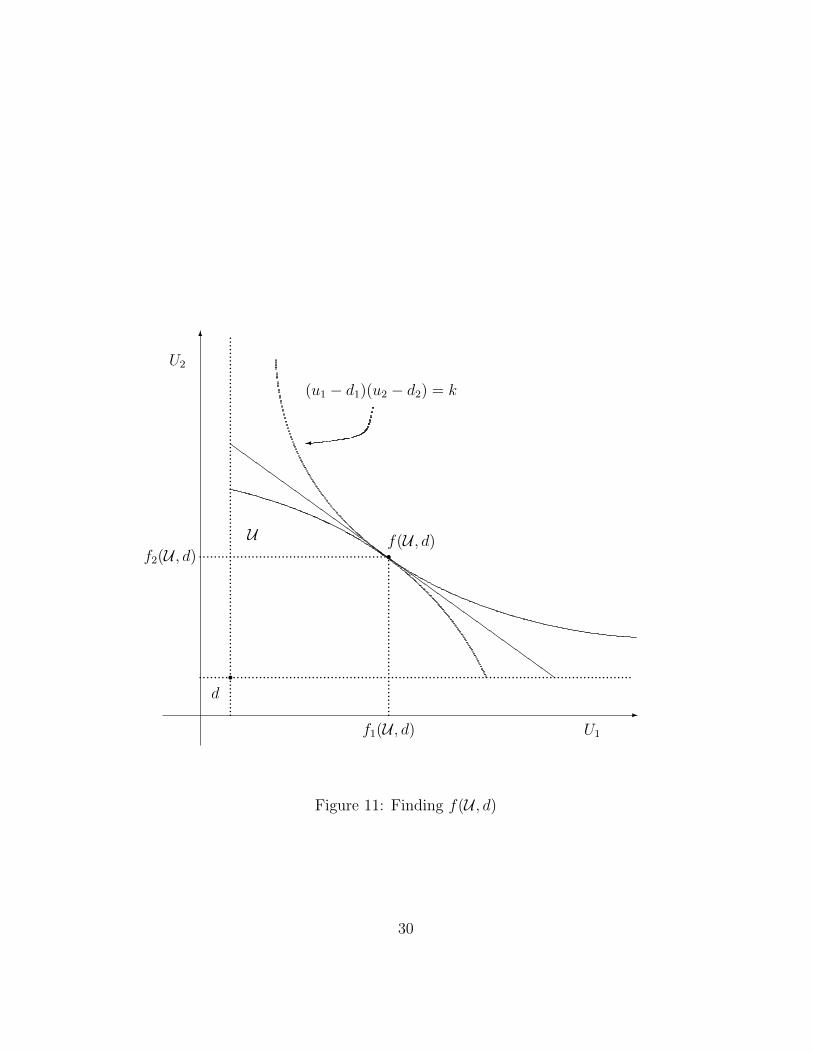
• This will give us a hyperbola that is tangent to U .
• So, if we look at the straight line that is tangent to the
hyperbola, it will also be tangent to U , at the same point.
• From what we have just worked out about tangents
to hyperbolae, the tangent to U will have just the right
property.
• The tangent to both U and the hyperbola will have
the property that the length of the two segments on
the tangent, from the tangency point to the vertical line
through d, and from the tangency point to the horizontal
line through d is the same. (See Figure 11.)
• It follows that f (U , d) must be the point of tangency
between U and the hyperbola. (See Figure 11.)
• Finding the furthest hyperbola from the origin with
asymptotes d1 and d2 that touches U is the geometric
equivalent of a constrained maximization prob-
lem.
• As k in (2.18) increases the hyperbola moves away from
the origin. Therefore we need to solve
27
maxu1,u2
(u1 − d1) (u2 − d2)
s.t. (u1, u2) ∈ U(2.19)
• The objective function in (2.19) is often called the
“Nash product.”
• To sum up, we have reached the following conclusion.
• Let a bargaining problem B = (U , d) be given.
• Assume that the solution function f satisfies PAR,
SYM, IUO, IUU and IIA.
• Denote by (u∗1, u∗2) the values of u1 and u2 that solve
the maximization problem (2.19).
• Then
f1(U , d) = u∗1 and f2(U , d) = u∗2 (2.20)
2.8 Canonical Example
•Consider again the canonical interpretation of 2.3 above.
• We pick specific utility functions for the buyer and the
seller.
28
6
-
U1
U2
.....................................................................................................
...........................................................................................................h
v
JJJJJJJJJJJJJJJ
rA
B
(u1 − v)(u2 − h) = k
�
Figure 10: Tangents to Hyperbola
29
6
-
U1
U2
rd
.....................................................................................................
...................................................................................................................
ZZZZZZZZZZZZZZZZZZZZZZZZZ
rU f(U , d)..............................................................................................
f1(U , d)
f2(U , d)
(u1 − d1)(u2 − d2) = k
�
Figure 11: Finding f(U , d)
30
• If the object is sold at price p, then
US(p− c) = (p− c)α (2.21)
and
UB(v − p) = (v − p)β (2.22)
• Remember that we are assuming that d1 = d2 = 0. If
there is no transaction the utility of both is zero.
• Remember that we are assuming that v > c. The
problem is not interesting otherwise.
• The “Nash product” therefore is
(p− c)α (v − p)β (2.23)
• So, we are looking for a p that maximizes (2.23), subject
to the agreement being feasible.
• So far we have written the constraint the the agreement
must be feasible as (u1, u2) ∈ U .
• In this case, there is an easy way to do this in terms of
price.
• The feasible utilities are the pairs
[(p− c)α, (v − p)β] (2.24)
as p varies in the interval [c, v].
• So, we should be maximizing (2.23) by choice of p,
subject to the constraint
c ≤ p ≤ v (2.25)
31
• We are going to try just maximizing (2.23) without
constraints.
• If we find a solution that satisfies (2.25), then this will
also be the solution to the constrained maximization
problem.
• Differentiating (2.23) wrt p and setting equal to 0 gives
α(p− c)α−1(v − p)β = β(p− c)α(v − p)β−1 (2.26)
• Dividing both sides of (2.26) by (p − c)α−1(v − p)β−1
gives
α(v − p) = β(p− c) (2.27)
• Solving (2.27) for p gives
p = vα
α + β+ c
β
α + β(2.28)
• Since both α and β are positive, the p in (2.28) clearly
satisfies (2.25).
• So, we are done. The price in (2.28) is the one at which
the exchange will take place.
• The price at which the exchange will take place is some-
where between c and v. Where in this interval depends
on the parameters of the buyer’s and seller’s utility func-
tions as specified in (2.28).
• As α becomes smaller (keeping β constant) the price
will get closer and closer to c.
32

• As β becomes smaller (keeping α constant) the price
will get closer and closer to v.
33


![[inria-00544527, v3] A Nash bargaining solution for ... · A Nash bargaining solution for Cooperative Network Formation Games 5 in link choices by any coalition is studied in [13]](https://img.pdfslide.us/doc/110x75/5f158219edf83e73541a843d/inria-00544527-v3-a-nash-bargaining-solution-for-a-nash-bargaining-solution.jpg)