ECON 4551 Econometrics II Memorial University of ... › ~rmartinezesp › ECON4551web › ch16... · Principles of Econometrics, 3rd Edition Slide16-13 P y GRADES>) P Eu ) P Eu2|

Qualitative and Limited Dependent Variable

Models

Adapted from Vera Tabakova’s notes

ECON 4551

Econometrics II

Memorial University of Newfoundland

16.1 Models with Binary Dependent Variables

16.2 The Logit Model for Binary Choice

16.3 Multinomial Logit

16.4 Conditional Logit

16.5 Ordered Choice Models

16.6 Models for Count Data

16.7 Limited Dependent Variables

Slide 16-2Principles of Econometrics, 3rd Edition

The choice options in multinomial and conditional logit models have

no natural ordering or arrangement. However, in some cases choices

are ordered in a specific way. Examples include:

1. Results of opinion surveys in which responses can be strongly

disagree, disagree, neutral, agree or strongly agree.

2. Assignment of grades or work performance ratings. Students receive

grades A, B, C, D, F which are ordered on the basis of a teacher’s

evaluation of their performance. Employees are often given

evaluations on scales such as Outstanding, Very Good, Good, Fair

and Poor which are similar in spirit.

Slide16-3Principles of Econometrics, 3rd Edition

When modeling these types of outcomes numerical values are

assigned to the outcomes, but the numerical values are ordinal, and

reflect only the ranking of the outcomes

The distance between the values is not meaningful!


Example:


1 strongly disagree

2 disagree

3 neutral

4 agree

5 strongly agree

y

The usual linear regression model is not appropriate for such data, because

in regression we would treat the y values as having some numerical

meaning when they do not.


(16.26)

3 4-year college (the full college experience)

2 2-year college (a partial college experience)

1 no college

y


*

i i iy GRADES e

*

2

*

1 2

*

1

3 (4-year college) if

2 (2-year college) if

1 (no college) if

i

i

i

y

y y

y

Figure 16.2 Ordinal Choices Relation to Thresholds



*

1 1

1

1

1i i i i

i i

i

P y P y P GRADES e

P e GRADES

GRADES


*

1 2 1 2

1 2

2 1

2i i i i

i i i

i i

P y P y P GRADES e

P GRADES e GRADES

GRADES GRADES


*

2 2

2

2

3

1

i i i i

i i

i

P y P y P GRADES e

P e GRADES

GRADES

The parameters are obtained by maximizing the log-likelihood

function using numerical methods. Most software includes options for

both ordered probit, which depends on the errors being standard

normal, and ordered logit, which depends on the assumption that the

random errors follow a logistic distribution.


1 2 1 2 3, , 1 2 3L P y P y P y

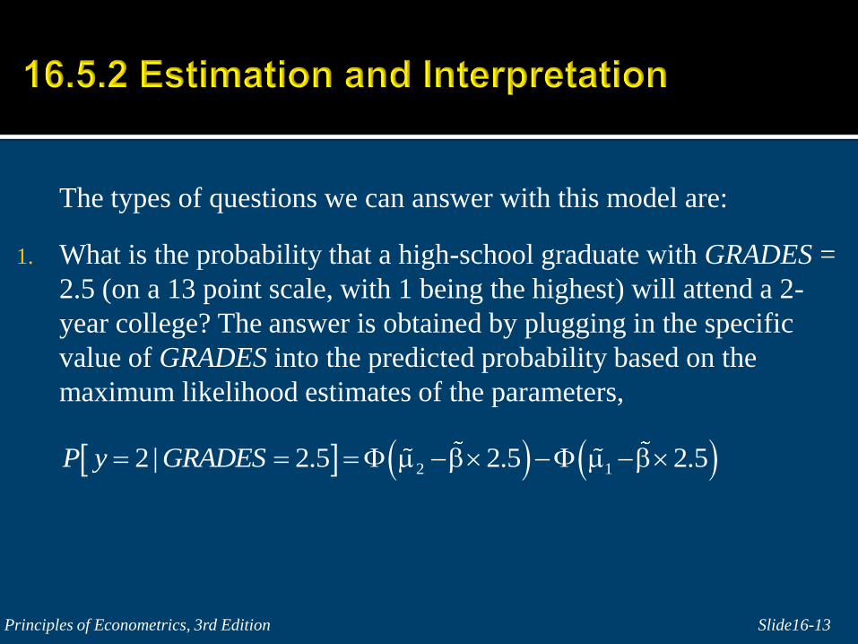
The types of questions we can answer with this model are:

1. What is the probability that a high-school graduate with GRADES =

2.5 (on a 13 point scale, with 1 being the highest) will attend a 2-

year college? The answer is obtained by plugging in the specific

value of GRADES into the predicted probability based on the

maximum likelihood estimates of the parameters,


2 12 | 2.5 2.5 2.5P y GRADES

2. What is the difference in probability of attending a 4-year college for

two students, one with GRADES = 2.5 and another with GRADES =

4.5? The difference in the probabilities is calculated directly as


2 | 4.5 2 | 2.5P y GRADES P y GRADES

3. If we treat GRADES as a continuous variable, what is the marginal

effect on the probability of each outcome, given a 1-unit change in

GRADES? These derivatives are:


1

1 2

2

1

2

3

P yGRADES

GRADES

P yGRADES GRADES

GRADES

P yGRADES

GRADES


Total 1,000 100.00 3 527 52.70 100.00 2 251 25.10 47.30 1 222 22.20 22.20 college Freq. Percent Cum. = 4-year college, 3 2-year = 1, 2 = no college

. tab psechoice

GRETL:

open "c:\Program Files\gretl\data\poe\nels_small.gdt"

probit psechoice const grades


# Marginal effects on probability of going to 4 year college

k = $ncoeff matrix b = $coeff[1:k-2] mu1 = $coeff[k-1] mu2 = $coeff[k]

matrix X = {6.64} scalar Xb = X*b P3a = pdf(N,mu2-Xb)*b (“N” stands for the normal distribution)

matrix X = 2.635 scalar Xb = X*b P3b = pdf(N,mu2-Xb)*b

printf "\nFor the median grade of 6.64, the marginal effect is %.4f\n", P3a

printf "\nFor the 5th percentile grade of 2.635, the marginal effect is %.4f\n", P3b



/cut2 -2.089993 .1357681 -2.356094 -1.823893 /cut1 -2.9456 .1468283 -3.233378 -2.657822 grades -.3066252 .0191735 -15.99 0.000 -.3442045 -.2690459 psechoice Coef. Std. Err. z P>|z| [95% Conf. Interval]

Log likelihood = -875.82172 Pseudo R2 = 0.1402 Prob > chi2 = 0.0000 LR chi2(1) = 285.67Ordered probit regression Number of obs = 1000

Iteration 3: log likelihood = -875.82172 Iteration 2: log likelihood = -875.82172 Iteration 1: log likelihood = -876.21962 Iteration 0: log likelihood = -1018.6575

. oprobit psechoice grades

Slide16-20


Log likelihood = -875.82172 Pseudo R2 = 0.1402 Prob > chi2 = 0.0000 LR chi2(1) = 285.67Ordered probit regression Number of obs = 1000

. oprobit psechoice grades, nolog

grades -.0537788 .00359 -14.99 0.000 -.060813 -.046745 2.635 variable dy/dx Std. Err. z P>|z| [ 95% C.I. ] X = .90008498 y = Pr(psechoice==3) (predict, outcome(3))Marginal effects after oprobit

. mfx, at(grades=2.635) predict(outcome(3))

grades -.1221475 .00763 -16.00 0.000 -.137108 -.107187 6.64 variable dy/dx Std. Err. z P>|z| [ 95% C.I. ] X = .52153319 y = Pr(psechoice==3) (predict, outcome(3))Marginal effects after oprobit


Slide16-21

Ordered Logit vs Ordered Probit

_cons -2.1 -3.5 cut2 _cons -2.9 -4.9 cut1 grades -.31 -.51 psechoice Variable oprobit ologit

. estimates table oprobit ologit, b(%7.2g) style(oneline)

Why is the second case more different than the first?

Ordered Logit vs Ordered Probit

grades -.0483174 .00348 -13.89 0.000 -.055136 -.041498 2.635 variable dy/dx Std. Err. z P>|z| [ 95% C.I. ] X = .89406527 y = Pr(psechoice==3) (predict, outcome(3))Marginal effects after ologit


grades -.1272801 .00844 -15.08 0.000 -.143827 -.110734 6.64 variable dy/dx Std. Err. z P>|z| [ 95% C.I. ] X = .52243824 y = Pr(psechoice==3) (predict, outcome(3))Marginal effects after ologit


Why is the second case more different than the first?

But remember that there is no meaningful numerical interpretation behind the values of the dependent variable in this model

There are many useful postestimations commands you should consider to understand and report your results (see, e.g. Long and Freese)

Ordered Logit is known as the proportional-odds model because the odds ratio of the event is independent of the category j. The odds ratio is assumed to be constant for all categories

These models assume that the effect of the slope coefficients on the switch from every category to the next is about the same

/cut2 -3.477195 .2416765 -3.950872 -3.003518 /cut1 -4.916916 .2672764 -5.440768 -4.393064 grades .6004068 .0203699 -15.04 0.000 .5617809 .6416884 psechoice Odds Ratio Std. Err. z P>|z| [95% Conf. Interval]

Log likelihood = -877.29561 Pseudo R2 = 0.1388 Prob > chi2 = 0.0000 LR chi2(1) = 282.72Ordered logistic regression Number of obs = 1000

. ologit psechoice grades, nolog or

You should test if the assumption is tenable This test is sensitive to the number of cases.

Samples with larger numbers of cases are more likely to show a statistically significant test

You should test if the assumption is tenable

Approximate likelihood-ratio test of proportionality of odds

across response categories:

chi2(1) = 0.18

Prob > chi2 = 0.6679

In standard STATA 9 for our example, too big for student version

regression assumption has been violated.A significant test statistic provides evidence that the parallel

grades 0.20 0.654 1 All 0.20 0.654 1 Variable chi2 p>chi2 df

Brant Test of Parallel Regression Assumption

. brant


Log likelihood = -877.29561 Pseudo R2 = 0.1388 Prob > chi2 = 0.0000 LR chi2(1) = 282.72Ordered logistic regression Number of obs = 1000

. ologit psechoice grades, nolog

A Wald test, that can identify the

Problem variables

regression assumption has been violated.A significant test statistic provides evidence that the parallel

grades 0.20 0.654 1 All 0.20 0.654 1 Variable chi2 p>chi2 df

Brant Test of Parallel Regression Assumption

_cons 5.11967 3.5222116grades -.53665426 -.51624365 y>1 y>2

Estimated coefficients from j-1 binary regressions

. brant, detail

If the assumption fails, you will have to consider other methods

Multinomial Logit Stereotype model (mclest in STATA) Generalized ordered logit model (gologit) Continuation ratio model Which are now becoming available in

commercial software

Slide 16-31Principles of Econometrics, 3rd Edition

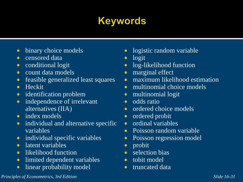
binary choice models censored data conditional logit count data models feasible generalized least squares Heckit identification problem independence of irrelevant

alternatives (IIA) index models individual and alternative specific

variables individual specific variables latent variables likelihood function limited dependent variables linear probability model

logistic random variable logit log-likelihood function marginal effect maximum likelihood estimation multinomial choice models multinomial logit odds ratio ordered choice models ordered probit ordinal variables Poisson random variable Poisson regression model probit selection bias tobit model truncated data

Survival analysis (time-to-event data analysis)

Multivariate probit (biprobit, triprobit, mvprobit)

Hoffmann, 2004 for all topics Long, S. and J. Freese for all topics Cameron and Trivedi’s book for count data

Agresti, A. (2001) Categorical Data Analysis(2nd ed). New York: Wiley.

Documents

ECON 4551 Econometrics II Memorial University of ... › ~rmartinezesp › ECON4551web › ch16... · Principles of Econometrics, 3rd Edition Slide16-13 P y GRADES>) P Eu ) P Eu2|