1

Econ 240A

Power Four

11

2

Last Time

• Probability

3

The Big Picture

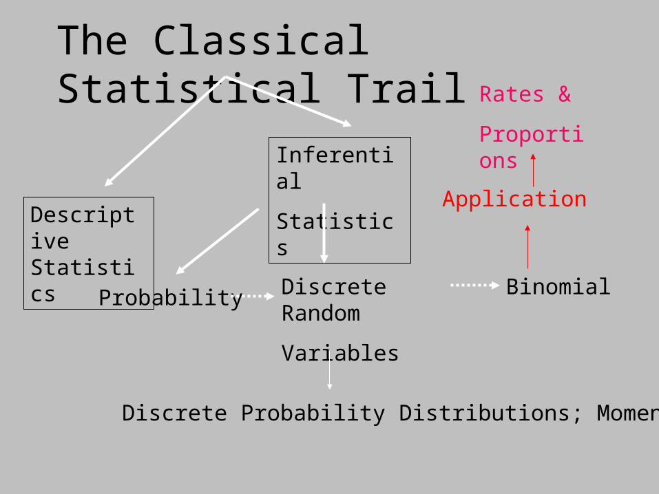
The Classical Statistical Trail

Descriptive Statistics

Inferential

Statistics

Probability Discrete Random

Variables

Discrete Probability Distributions; Moments

Binomial

Application

Rates &

Proportions

5

9

Working Problems

10

Problem 6.61

• A survey of middle aged men reveals that 28% of them are balding at the crown of their head. Moreover, it is known that such men have an 18% probability of suffering a heart attack in the next ten years. Men who are not balding in this way have an 11% probability of a heart attack. Find the probability that a middle aged man will suffer a heart attack in the next ten years.

11

Middle Aged men

Bald

P (Bald and MA) = 0.28

Not Bald

12

Middle Aged men

Bald

P (Bald and MA) = 0.28

Not Bald

P(HA/Bald and MA) = 0.18

P(HA/Not Bald and MA)= 0.11

13

Probability of a heart attack in the next ten

years• P(HA) = P(HA and Bald and MA) +

P(HA and Not Bald and MA)• P(HA) = P(HA/Bald and

MA)*P(BALD and MA) + P(HA/Not BALD and MA)* P(Not Bald and MA)

• P(HA) = 0.18*0.28 + 0.11*0.72 = 0.054 + .0792 = 0.1296

14

This time

15

Random Variables

• There is a natural transition or easy segue from our discussion of probability and Bernoulli trials last time to random variables

• Define k to be the random variable # of heads in 1 flip, 2 flips or n flips of a coin

• We can find the probability that k=0, or k=n by brute force using probability trees. We can find the histogram for k, its central tendency and its dispersion

16

Outline

• Random Variables & Bernoulli Trials• example: one flip of a coin

– expected value of the number of heads– variance in the number of heads

• example: two flips of a coin• a fair coin: frequency distribution of the

number of heads– one flip– two flips

17

Outline (Cont.)

• Three flips of a fair coin, the number of combinations of the number of heads

• The binomial distribution• frequency distributions for the binomial• The expected value of a discrete

random variable• the variance of a discrete random

variable

18

Concept

• Bernoulli Trial– two outcomes, e.g. success or failure– successive independent trials– probability of success is the same in

each trial

• Example: flipping a coin multiple times

19

Flipping a Coin Once

Heads, k=1

Tails, k=0

Prob. = p

Prob. = 1-p

The random variable k is the number of headsit is variable because k can equal one or zeroit is random because the value of k depends on probabilities of occurrence, p and 1-p

20

Flipping a coin once

• Expected value of the number of heads is the value of k weighted by the probability that value of k occurs– E(k) = 1*p + 0*(1-p) = p

• variance of k is the value of k minus its expected value, squared, weighted by the probability that value of k occurs– VAR(k) = (1-p)2 *p +(0-p)2 *(1-p) =

VAR(k) = (1-p)*p[(1-p)+p] =(1-p)*p

21

Flipping a coin twice: 4 elementary outcomes

heads

tails

heads

tails

heads

tails

h, h

h, t

t, h

t, t

h, h; k=2

h, t; k=1

t, h; k=1

t, t; k=0

Prob =p

Prob =p

Prob =1-p

Prob =1-p

Prob=p

Prob=1-p

22

Flipping a Coin Twice

• Expected number of heads– E(k)=2*p2 +1*p*(1-p) +1*(1-p)*p + 0*(1-

p)2 E(k) = 2*p2 + p - p2 + p - p2 =2p– so we might expect the expected value of

k in n independent flips is n*p

• Variance in k– VAR(k) = (2-2p)2 *p2 + 2*(1-2p)2 *p(1-p) +

(0-2p)2 (1-p)2

23

Continuing with the variance in k

– VAR(k) = (2-2p)2 *p2 + 2*(1-2p)2 *p(1-p) + (0-2p)2 (1-p)2

– VAR(k) = 4(1-p)2 *p2 +2*(1 - 4p +4p2)*p*(1-p) + 4p2 *(1-p)2

– adding the first and last terms, 8p2 *(1-p)2 + 2*(1 - 4p +4p2)*p*(1-p)

– and expanding this last term, 2p(1-p) -8p2 *(1-p) + 8p3 *(1-p)

– VAR(k) = 8p2 *(1-p)2 + 2p(1-p) -8p2 *(1-p)(1-p)– so VAR(k) = 2p(1-p) , or twice VAR(k) for 1 flip

24

• So we might expect the variance in n flips to be np(1-p)

25

Frequency Distribution for the Number of Heads

• A fair coin

26

O heads 1 head

1/2

probability

# of heads

One Flip of the Coin

27

0 1 2 # of heads

probability

1/4

1/2

Two Flips of a Fair Coin

28

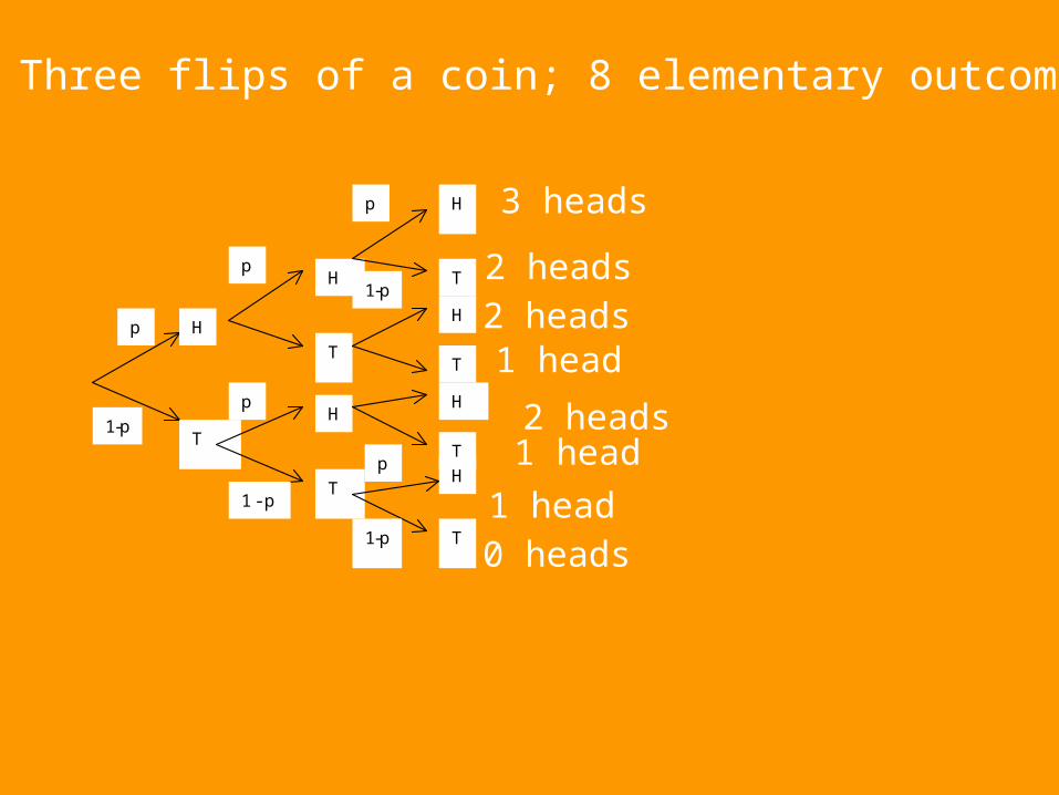
Three Flips of a Fair Coin

• It is not so hard to see what the value of the number of heads, k, might be for three flips of a coin: zero, one ,two, three

• But one head can occur two ways, as can two heads

• Hence we need to consider the number of ways k can occur, I.e. the combinations of branching probabilities where order does not count

H

T

H

T

p

H

T

1-p

p

1 - p

p

H

T

H

T

H

T

H

T

p

1-p

p

1-p

Three flips of a coin; 8 elementary outcomes

3 heads

2 heads

2 heads1 head

2 heads1 head

1 head

0 heads

30

Three Flips of a Coin

• There is only one way of getting three heads or of getting zero heads

• But there are three ways of getting two heads or getting one head

• One way of calculating the number of combinations is Cn(k) = n!/k!*(n-k)!

• Another way of calculating the number of combinations is Pascal’s triangle

31

32

0 1 2

1/8

2/8

3/8

Probability

3 # of heads

Three Flips of a Coin

33

The Probability of Getting k Heads

• The probability of getting k heads (along a given branch) in n trials is: pk *(1-p)n-k

• The number of branches with k heads in n trials is given by Cn(k)

• So the probability of k heads in n trials is Prob(k) = Cn(k) pk *(1-p)n-k

• This is the discrete binomial distribution where k can only take on discrete values of 0, 1, …k

Expected Value of a discrete random variable

• E(x) =

• the expected value of a discrete random variable is the weighted average of the observations where the weight is the frequency of that observation

n

i

ixpix0

)]([*)(

35

Expected Value of the sum of random variables

• E(x + y) = E(x) + E(y)

Expected Number of Heads After Two Flips

• Flip One: kiI heads

• Flip Two: kjII heads

• Because of independence p(kiI and kj

II) = p(ki

I)*p(kjII)

• Expected number of heads after two flips: E(ki

I + kjII) = (ki

I + kjII)

p(kiI)*p(kj

II)

• E(kiI + kj

II) = kiI p(ki

I)* p(kjII) +

1

0

1

0 ji

1

0i

1

0j

Cont.

• E(kiI + kj

II) = kiI p(ki

I)* p(kjII)

+ kjII *p(kj

II) p(kiI)

• E(kiI + kj

II) = E(kiI) + E(kj

II) = p*1 + p*1 =2p

• So the mean after n flips is n*p

1

0i

1

0j

1

0j

1

0i

Variance of a discrete random variable

• VAR(xi) =

• the variance of a discrete random variable is the weighted sum of each observation minus its expected value, squared,where the weight is the frequency of that observation

)]([})]([)({[ 2

0

ixpixEixn

i

Cont.

• VAR(xi) =

• VAR(xi) =

• VAR(xi) =

• So the variance equals the second moment minus the first moment squared

)]([*})]([)({ 2

0

ixpixEixn

i

})([*})]([)(*)]([2)]({[0

22

n

i

ixpiExixixEix

2

0

2 )]([)]}([)]([{ ixEixpixn

i

The variance of the sum of discrete random variables

• VAR[xi + yj] = E[xi + yj - E(xi + yj)]2

• VAR[xi + yj] = E[(xi - Exi) + (yj - Eyj)]2

• VAR[xi + yj] = E[(xi - Exi)2 + 2(xi - Exi) (yj - Eyj) + (yj - Eyj)2]

• VAR[xi + yj] = VAR[xi] + 2 COV[xi*yj] + VAR[yj]

The variance of the sum if x and y are independent

• COV [xi*yj] = E(xi - Exi) (yj - Eyj)

• COV [xi*yj]= (xi - Exi) (yj - Eyj)

• COV [xi*yj]= (xi - Exi) p[x(i)]* (yj - Eyj)* p[y(j)]

• COV [xi*yj] = 0

)]()([ jyixp

n

j

m

i 00

m

i 0

n

j 0

42

Variance of the number of heads after two flips

• Since we know the variance of the number of heads on the first flip is p*(1-p)

• and ditto for the variance in the number of heads for the second flip

• then the variance in the number of heads after two flips is the sum, 2p(1-p)

• and the variance after n flips is np(1-p)

43

Application

• Rates and Proportions

Field Poll

• The estimated proportion, from the sample, that will vote for Prop. 74 is:

• where is 0.46 or 46%• k is the number of “successes”, the

number of likely voters sampled who are for Prop 74, approximately 144

• n is the size of the sample, 314

nkp /ˆ

p̂

Field Poll

• What is the expected proportion of voters Nov. 2 that will vote for Prop 74?

• = E(k)/n = np/n = p, where from the binomial distribution, E(k) = np

• So if the sample is representative of voters and their preferences, 46% should vote for Prop. 74 next November

)ˆ( pE

Field Poll

• How much dispersion is in this estimate, i.e. as reported in newspapers, what is the margin of sampling error?

• The margin of sampling error is calculated as the standard deviation or square root of the variance in

• = VAR(k)/n2 = np(1-p)/n2 =p(1-p)/n

• and using 0.46 as an estimate of p,• = 0.46*0.54/314 =0.000791

p̂

)ˆ( pVAR

)ˆ( pVAR

49

Field Poll

• So the sampling error should be 0.028 or 2.8%, i.e. the square root of 0.000791

• The Field Poll reports a 95% confidence interval or about two standard errors , I.e 2*2.8% = 5.6%

50

Field Poll

• Is it possible that Prop 74 could win? This estimate of 0.46 plus or minus twice the sampling error of 0.028, creates an interval of 0.40 to 0. 52

• Based on a normal approximation to the binomial, the true proportion voting for Prop.74 should fall in this interval with probability of about 95%, unless sentiments change.

51

Lab Two

• The Binomial Distribution, Numbers & Plots– Coin flips: one, two, …ten– Die Throws: one, ten ,twenty

• The Normal Approximation to the Binomial