Econ 240 C

Lecture 16

2

Part I. ARCH-M Modeks

In an ARCH-M model, the conditional variance is introduced into the equation for the mean as an explanatory variable.

ARCH-M is often used in financial models

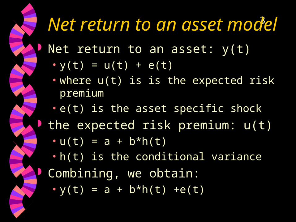
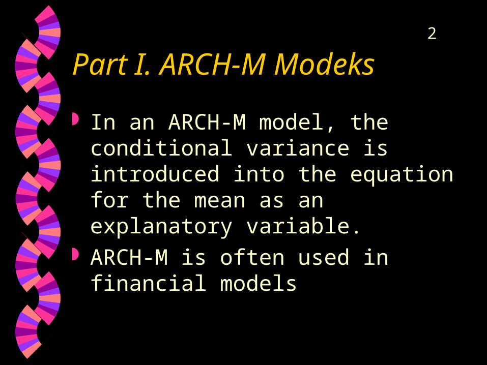
3Net return to an asset model Net return to an asset: y(t)

• y(t) = u(t) + e(t)• where u(t) is is the expected risk premium• e(t) is the asset specific shock

the expected risk premium: u(t)• u(t) = a + b*h(t)• h(t) is the conditional variance

Combining, we obtain:• y(t) = a + b*h(t) +e(t)

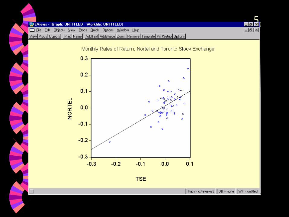
4Northern Telecom And Toronto Stock Exchange

Nortel and TSE monthly rates of return on the stock and the market, respectively

Keller and Warrack, 6th ed. Xm 18-06 data file

We used a similar file for GE and S_P_Index01 last Fall in Lab 6 of Econ 240A

5

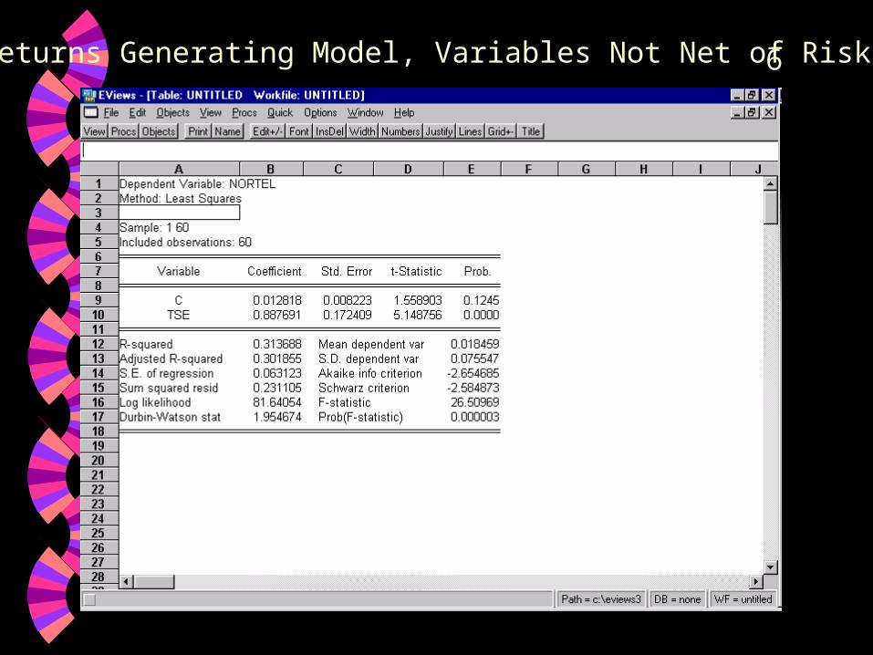
6Returns Generating Model, Variables Not Net of Risk Free

7

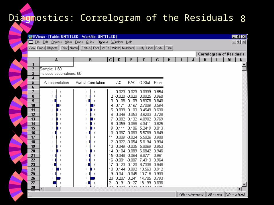
8Diagnostics: Correlogram of the Residuals

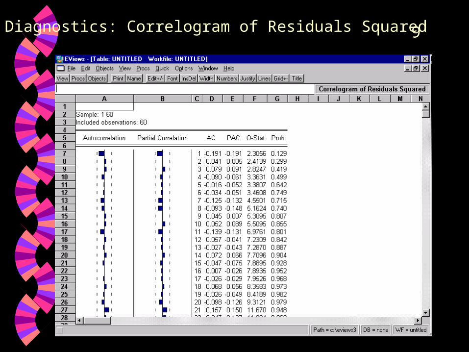
9Diagnostics: Correlogram of Residuals Squared

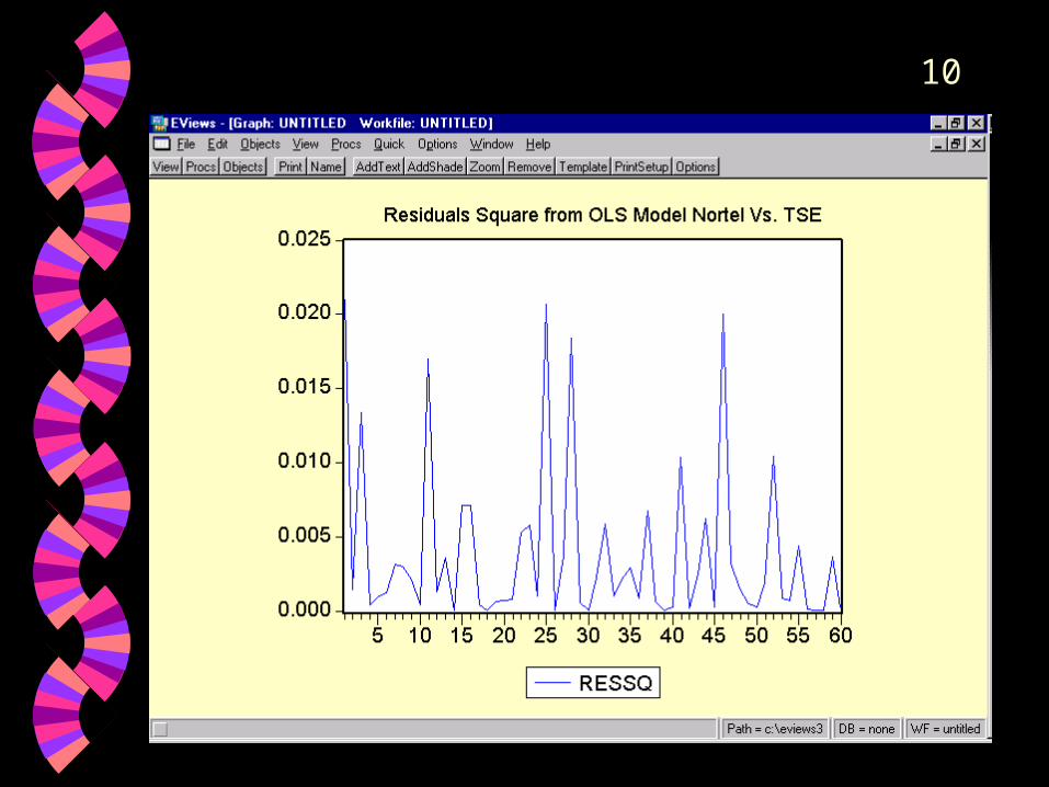
10

11Try Estimating An ARCH-

GARCH Model

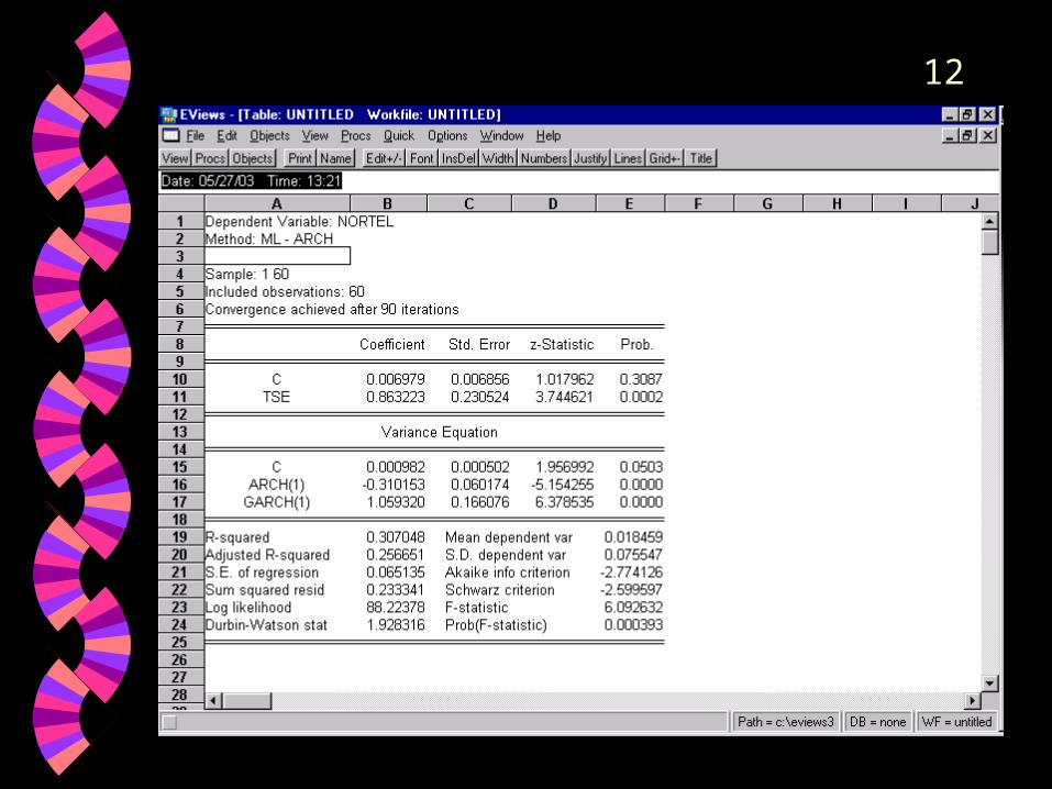
12

13Try Adding the Conditional Variance to the Returns Model PROCS: Make GARCH variance series:

GARCH01 series

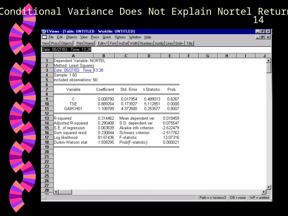
14Conditional Variance Does Not Explain Nortel Return

15

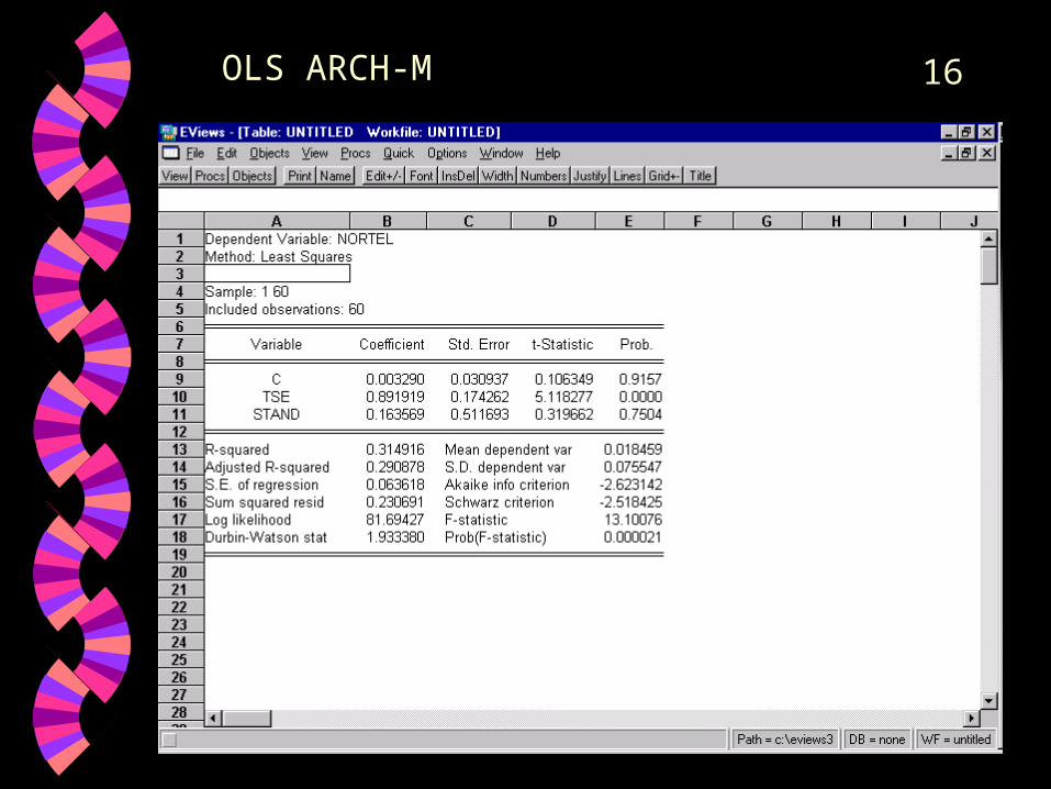
16OLS ARCH-M

17

Estimate ARCH-M Model

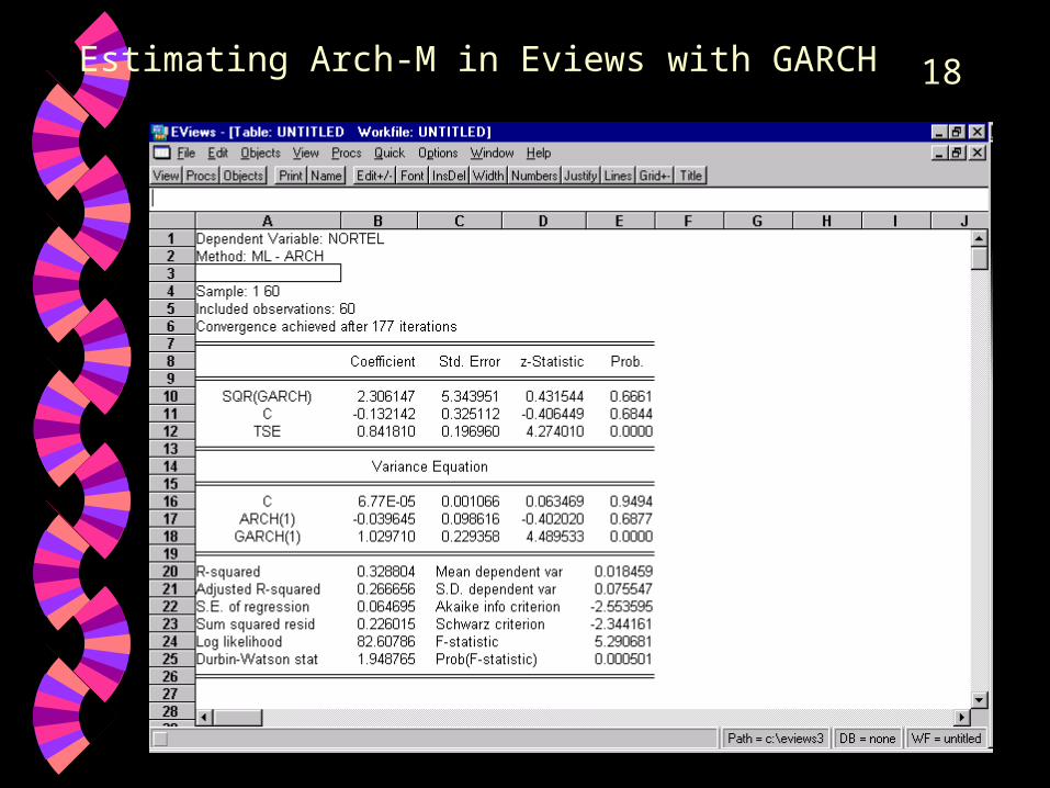
18Estimating Arch-M in Eviews with GARCH

19

Part II. Granger Causality

Granger causality is based on the notion of the past causing the present

example: Lab six, Index of Consumer Sentiment January 1978 - March 2003 and S&P500 total return, montly January 1970 - March 2003

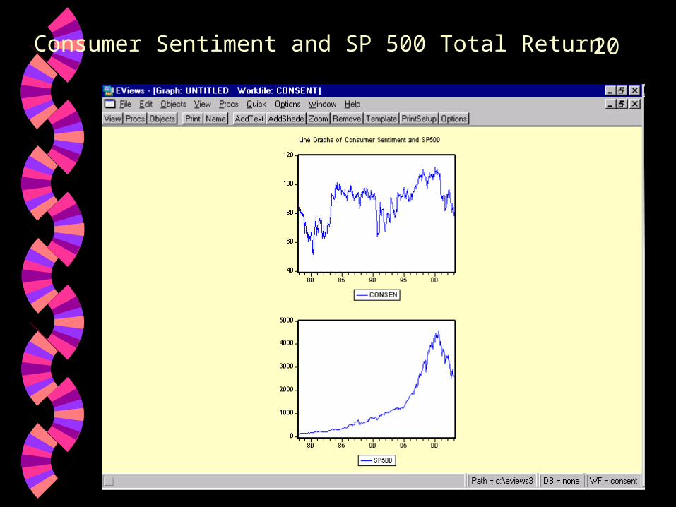
20Consumer Sentiment and SP 500 Total Return

21

Time Series are Evolutionary

Take logarithms and first difference

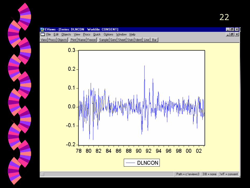
22

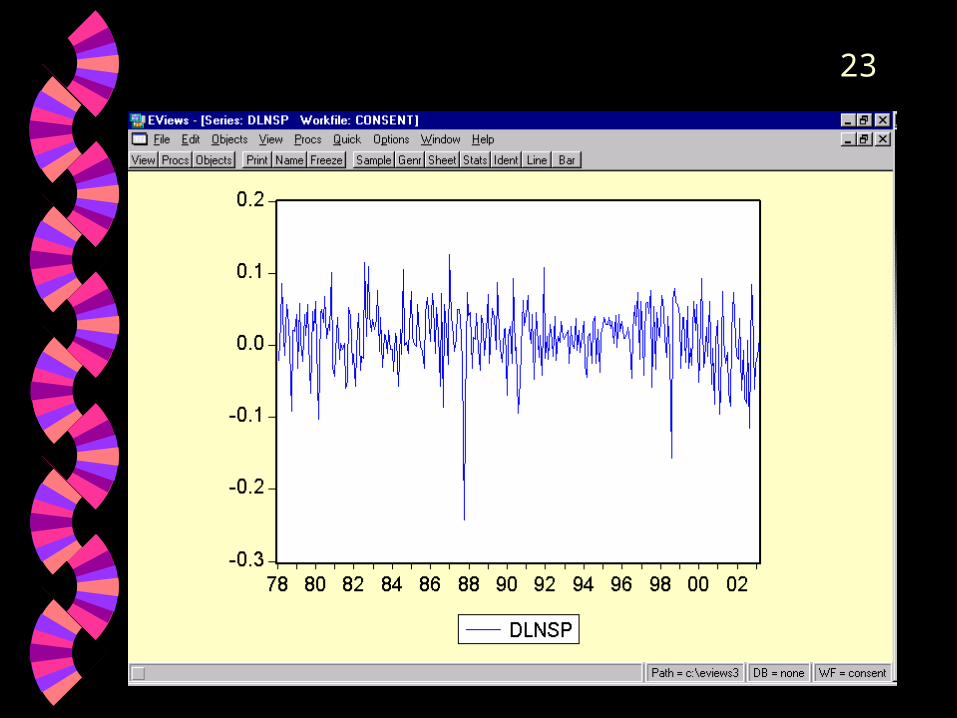
23

24

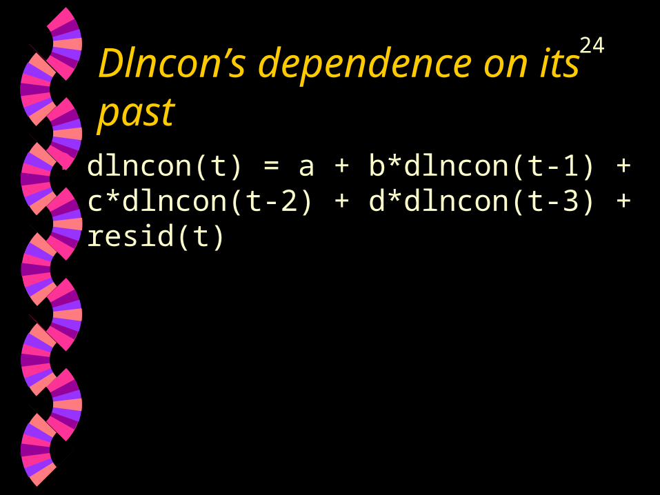
Dlncon’s dependence on its past

dlncon(t) = a + b*dlncon(t-1) + c*dlncon(t-2) + d*dlncon(t-3) + resid(t)

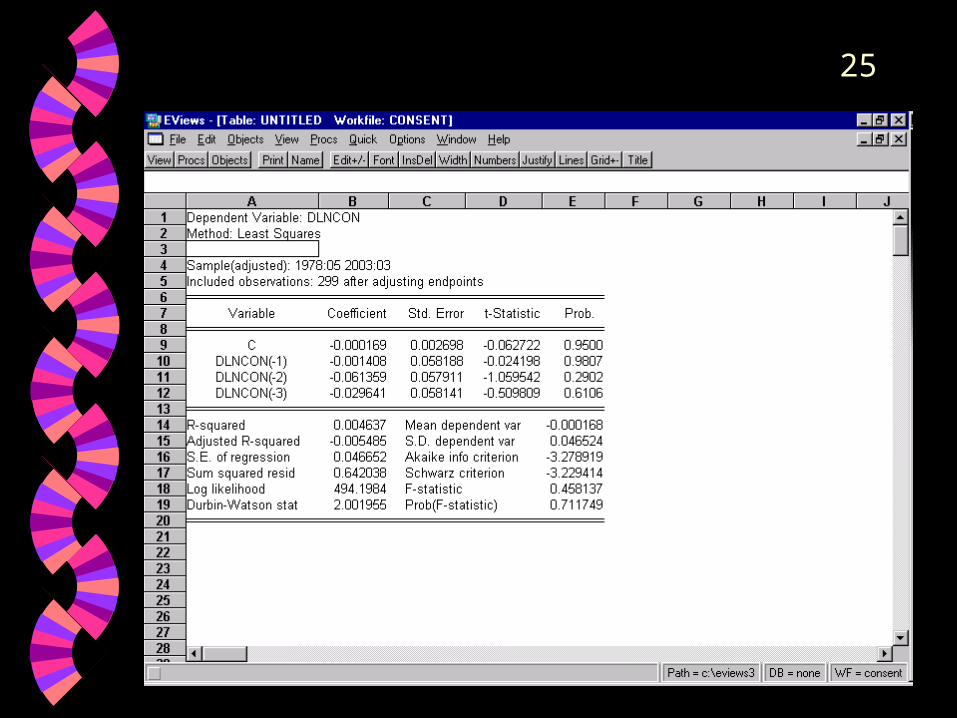
25

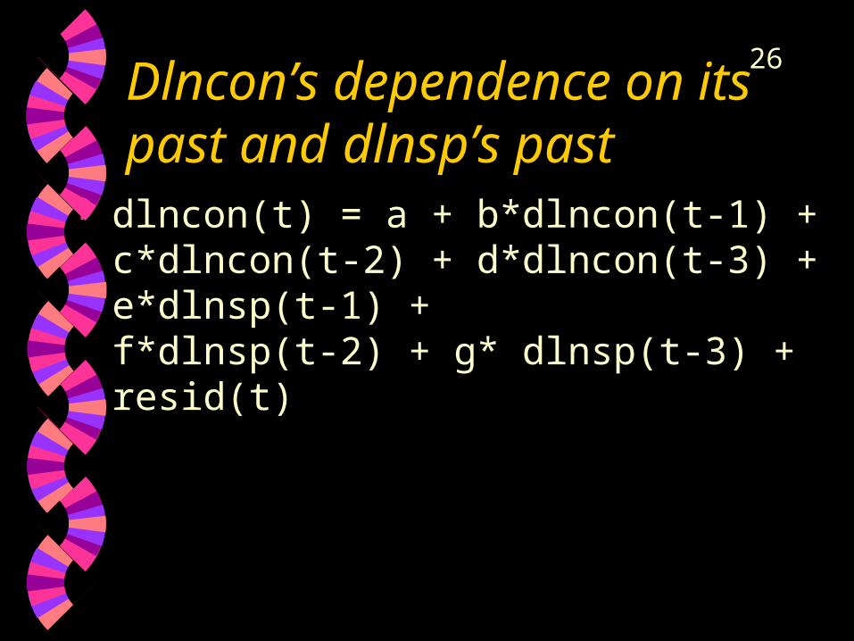
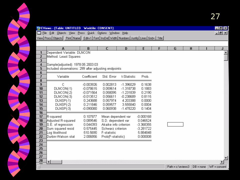
26Dlncon’s dependence on its past and dlnsp’s past

dlncon(t) = a + b*dlncon(t-1) + c*dlncon(t-2) + d*dlncon(t-3) + e*dlnsp(t-1) + f*dlnsp(t-2) + g* dlnsp(t-3) + resid(t)

27

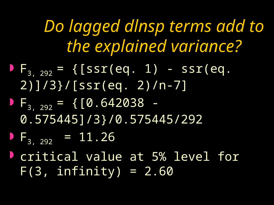
Do lagged dlnsp terms add to the explained variance?

F3, 292 = {[ssr(eq. 1) - ssr(eq. 2)]/3}/[ssr(eq. 2)/n-7]

F3, 292 = {[0.642038 - 0.575445]/3}/0.575445/292

F3, 292 = 11.26

critical value at 5% level for F(3, infinity) = 2.60

29

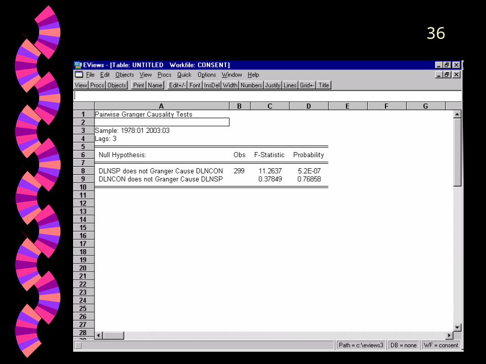
Causality goes from dlnsp to dlncon

EVIEWS Granger Causality Test• open dlncon and dlnsp• go to VIEW menu and select Granger Causality• choose the number of lags

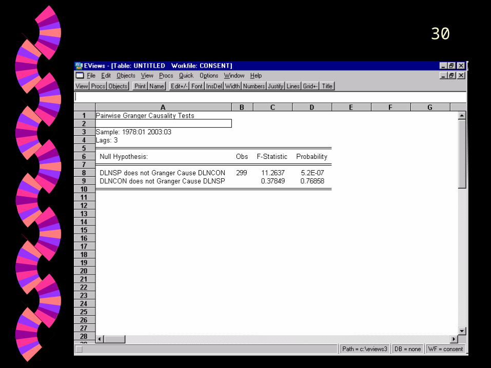
30

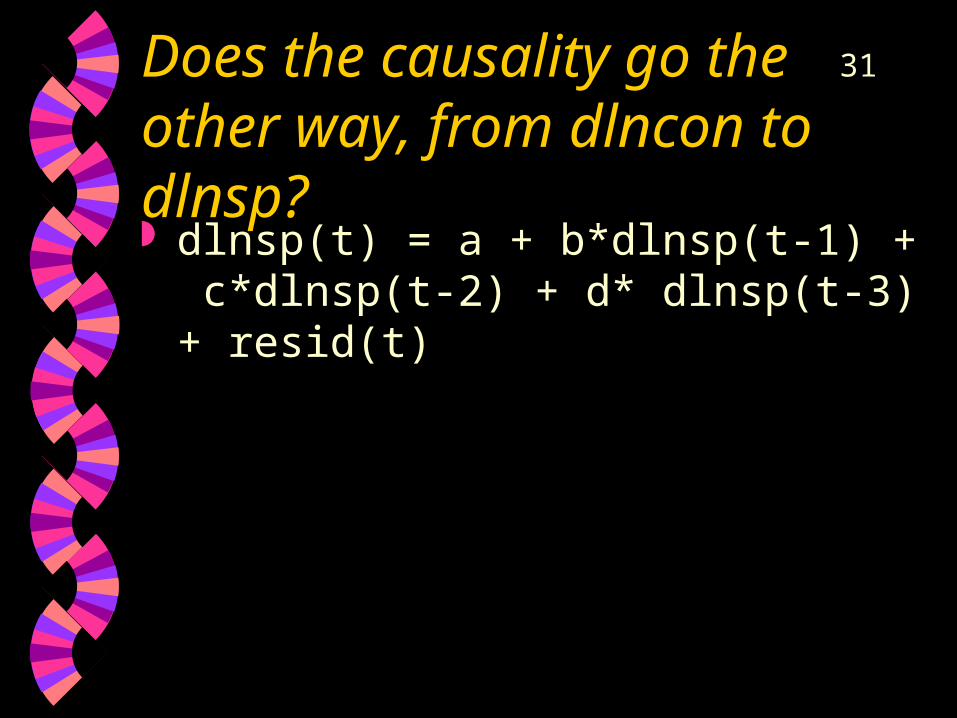
31Does the causality go the other way, from dlncon to dlnsp? dlnsp(t) = a + b*dlnsp(t-1) + c*dlnsp(t-2) +

d* dlnsp(t-3) + resid(t)

32

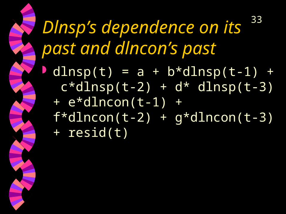
33Dlnsp’s dependence on its past and dlncon’s past dlnsp(t) = a + b*dlnsp(t-1) + c*dlnsp(t-2) +

d* dlnsp(t-3) + e*dlncon(t-1) + f*dlncon(t-2) + g*dlncon(t-3) + resid(t)

34

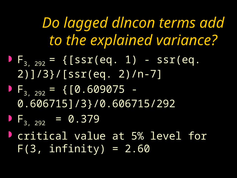
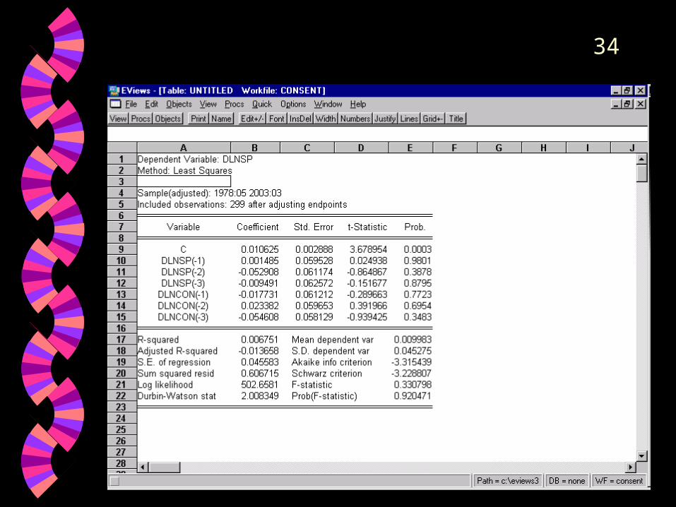
Do lagged dlncon terms add to the explained variance?

F3, 292 = {[ssr(eq. 1) - ssr(eq. 2)]/3}/[ssr(eq. 2)/n-7]

F3, 292 = {[0.609075 - 0.606715]/3}/0.606715/292

F3, 292 = 0.379

critical value at 5% level for F(3, infinity) = 2.60

36

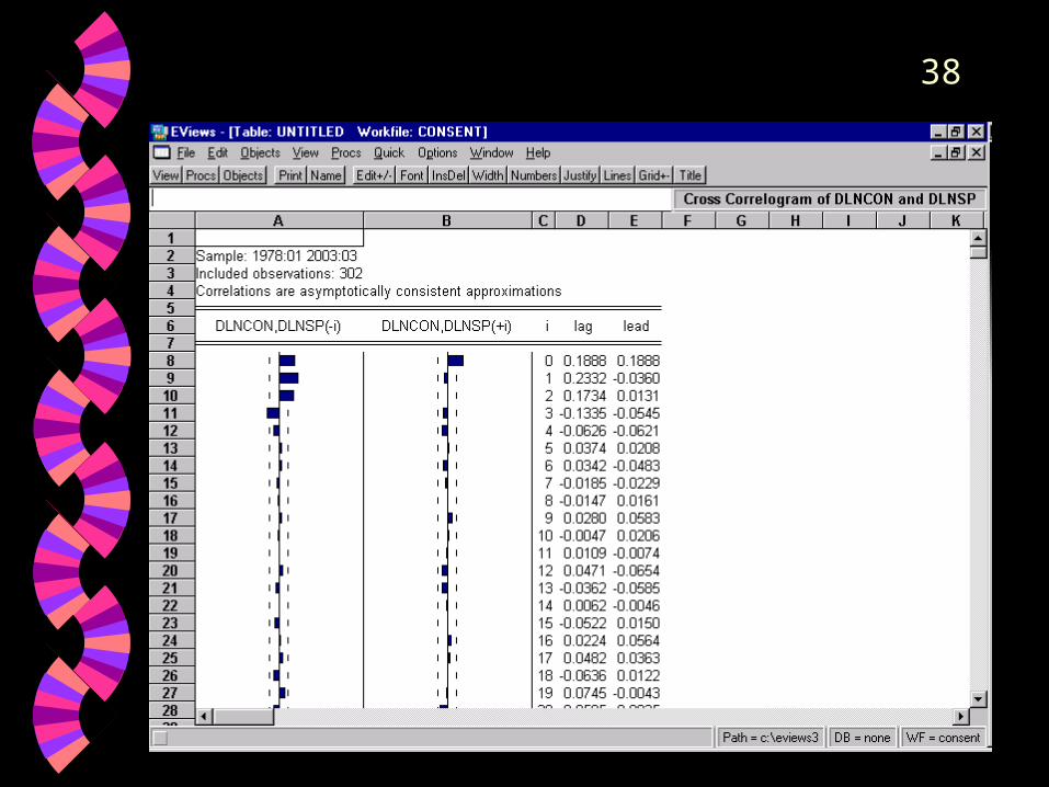
37Granger Causality and Cross-Correlation

One-way causality from dlnsp to dlncon reinforces the results inferred from the cross-correlation function

38

39Part III. Simultaneous Equations

and Identification Lecture 2, Section I Econ 240C Spring

2004 Sometimes in microeconomics it is possible

to identify, for example, supply and demand, if there are exogenous variables that cause the curves to shift, such as weather (rainfall) for supply and income for demand

40

Demand: p = a - b*q +c*y + ep

41

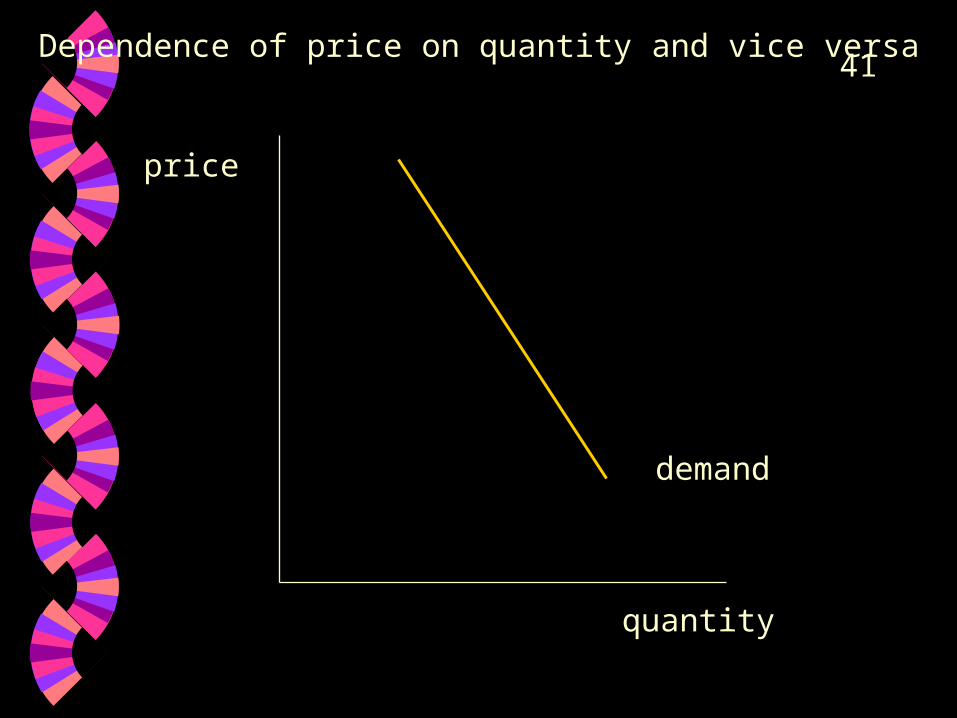
demand

price

quantity

Dependence of price on quantity and vice versa

42

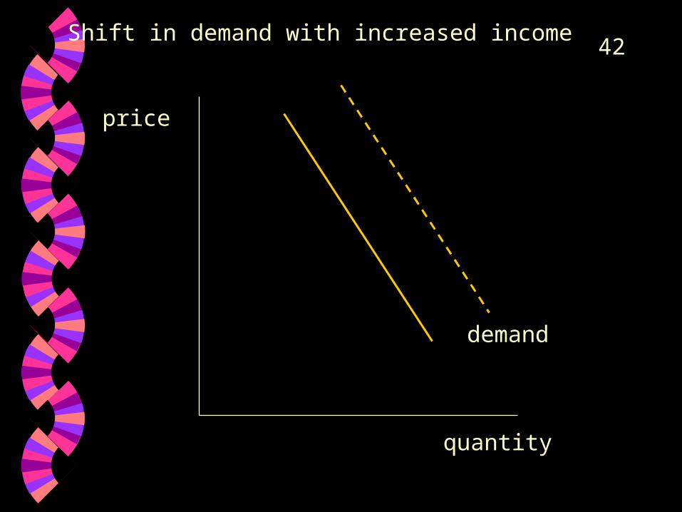
demand

price

quantity

Shift in demand with increased income

43

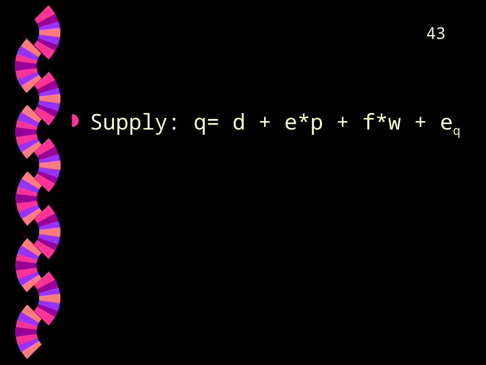
Supply: q= d + e*p + f*w + eq

44

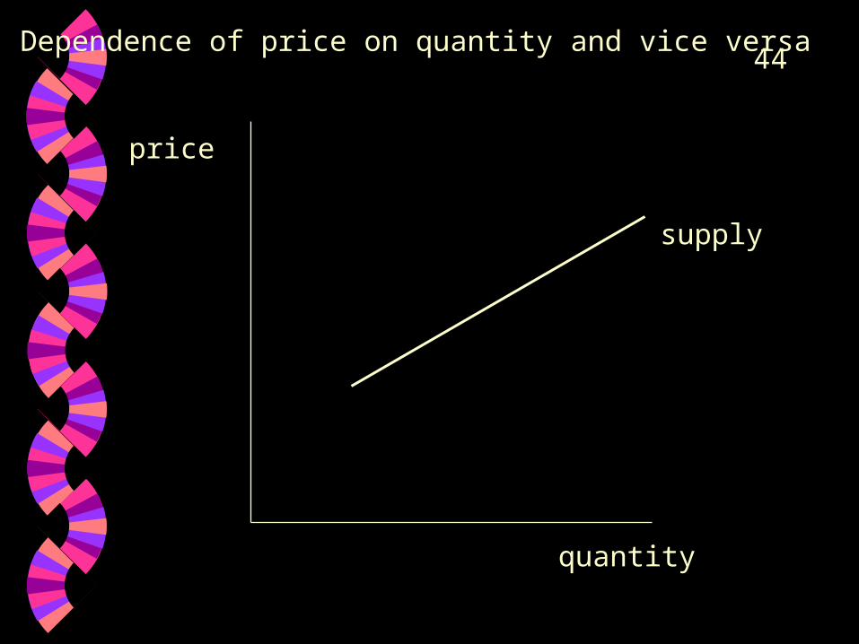
price

quantity

supply

Dependence of price on quantity and vice versa

45

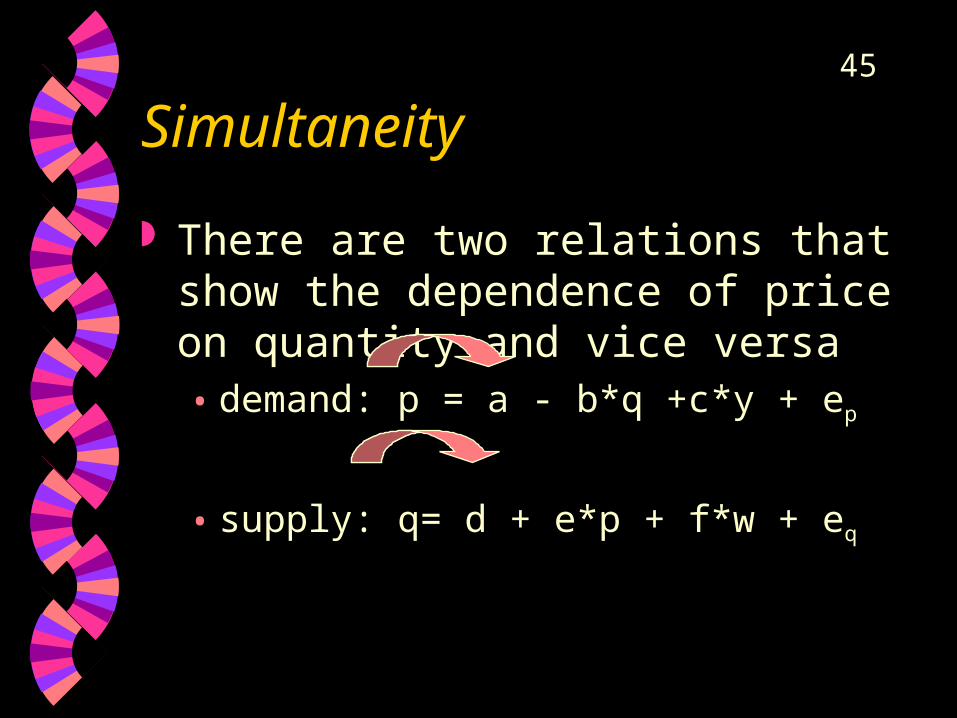
Simultaneity

There are two relations that show the dependence of price on quantity and vice versa• demand: p = a - b*q +c*y + ep

• supply: q= d + e*p + f*w + eq

46

Endogeneity

Price and quantity are mutually determined by demand and supply, i.e. determined internal to the model, hence the name endogenous variables

income and weather are presumed determined outside the model, hence the name exogenous variables

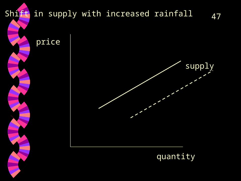
47

price

quantity

supply

Shift in supply with increased rainfall

48

Identification

Suppose income is increasing but weather is staying the same

49

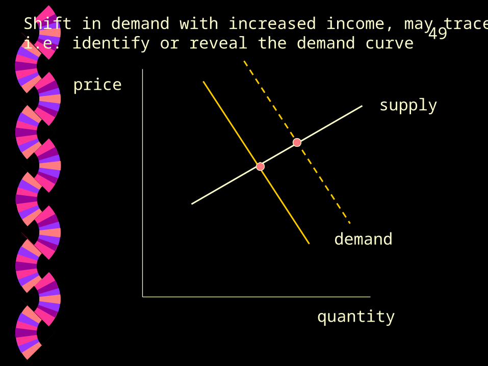
demand

price

quantity

Shift in demand with increased income, may trace outi.e. identify or reveal the demand curve

supply

50

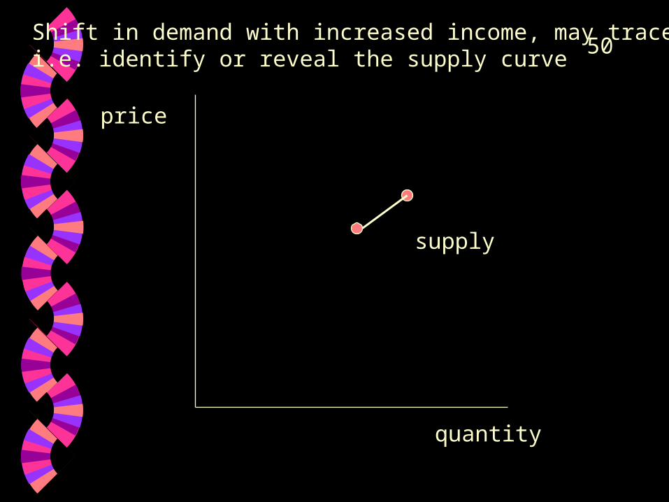
price

quantity

Shift in demand with increased income, may trace outi.e. identify or reveal the supply curve

supply

51

Identification

Suppose rainfall is increasing but income is staying the same

52

price

quantity

supply

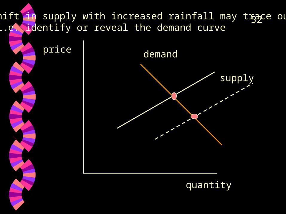
Shift in supply with increased rainfall may trace out, i.e. identify or reveal the demand curve

demand

53

price

quantity

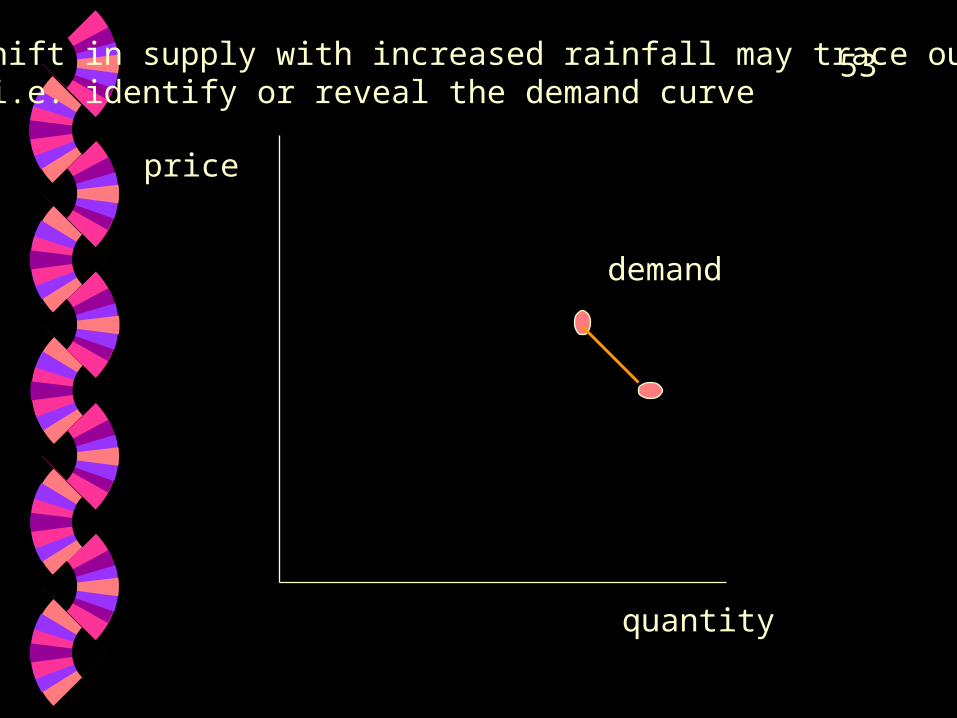
Shift in supply with increased rainfall may trace out, i.e. identify or reveal the demand curve

demand

54

Identification

Suppose both income and weather are changing

55

price

quantity

supply

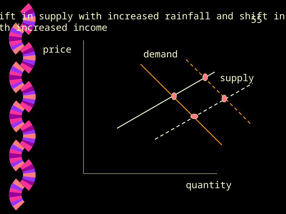
Shift in supply with increased rainfall and shift in demandwith increased income

demand

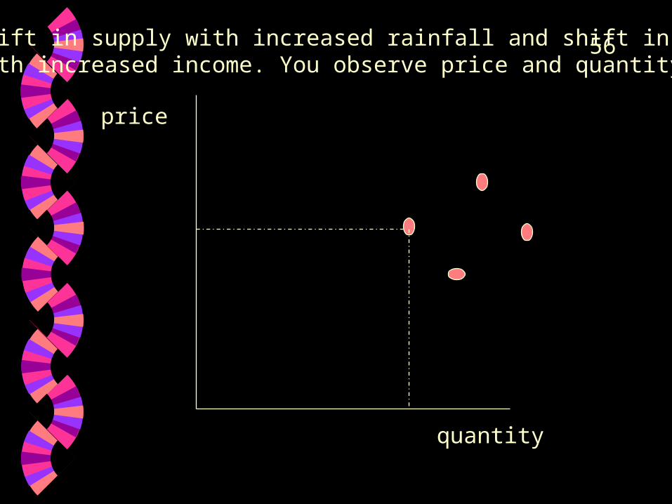
56

price

quantity

Shift in supply with increased rainfall and shift in demandwith increased income. You observe price and quantity

57

Identification

All may not be lost, if parameters of interest such as a and b can be determined from the dependence of price on income and weather and the dependence of quantity on income and weather then the demand model can be identified and so can supply

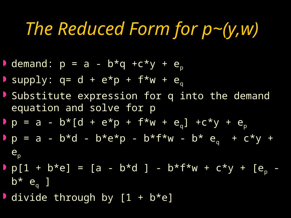
The Reduced Form for p~(y,w)

demand: p = a - b*q +c*y + ep

supply: q= d + e*p + f*w + eq

Substitute expression for q into the demand equation and solve for p

p = a - b*[d + e*p + f*w + eq] +c*y + ep

p = a - b*d - b*e*p - b*f*w - b* eq + c*y + ep

p[1 + b*e] = [a - b*d ] - b*f*w + c*y + [ep - b* eq ]

divide through by [1 + b*e]

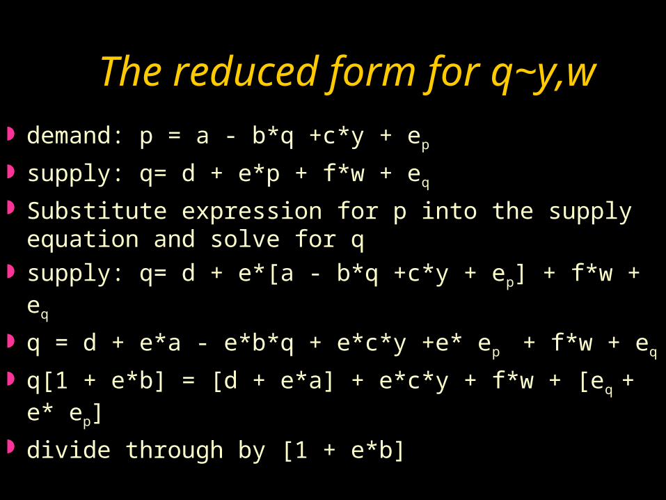
The reduced form for q~y,w

demand: p = a - b*q +c*y + ep

supply: q= d + e*p + f*w + eq

Substitute expression for p into the supply equation and solve for q

supply: q= d + e*[a - b*q +c*y + ep] + f*w + eq

q = d + e*a - e*b*q + e*c*y +e* ep + f*w + eq

q[1 + e*b] = [d + e*a] + e*c*y + f*w + [eq + e* ep]

divide through by [1 + e*b]

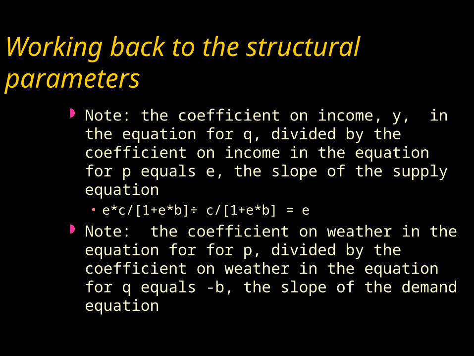
Working back to the structural parameters

Note: the coefficient on income, y, in the equation for q, divided by the coefficient on income in the equation for p equals e, the slope of the supply equation• e*c/[1+e*b]÷ c/[1+e*b] = e

Note: the coefficient on weather in the equation for for p, divided by the coefficient on weather in the equation for q equals -b, the slope of the demand equation

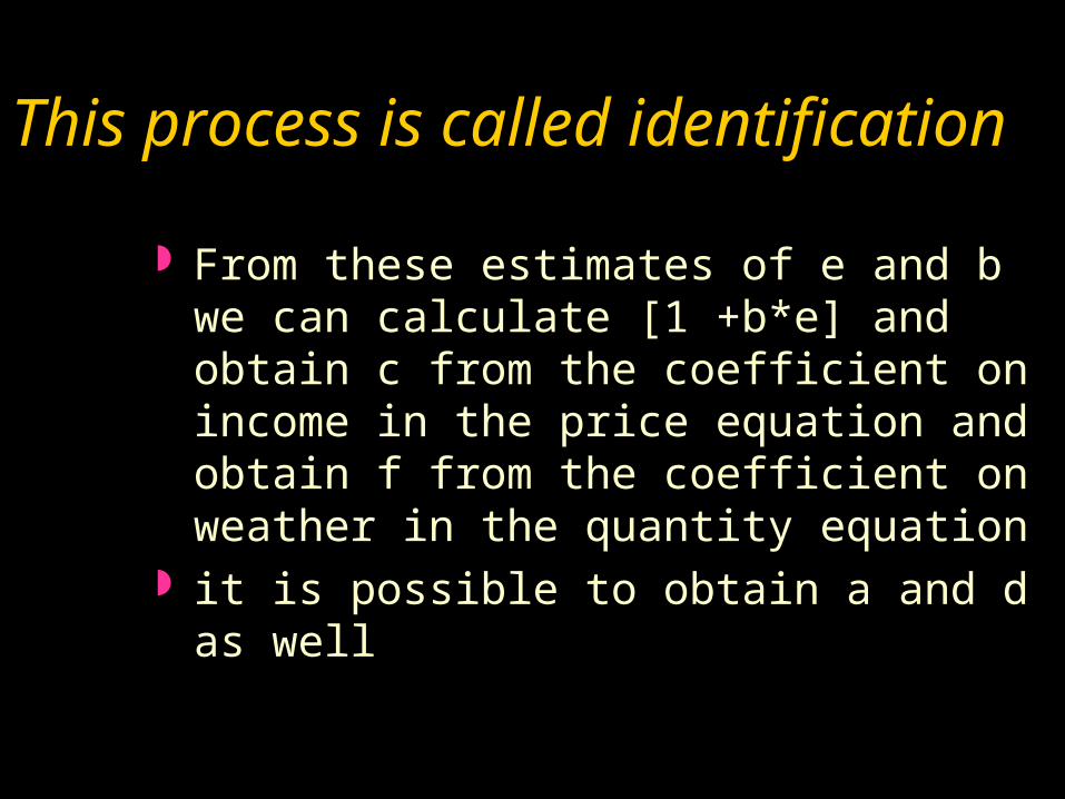
This process is called identification

From these estimates of e and b we can calculate [1 +b*e] and obtain c from the coefficient on income in the price equation and obtain f from the coefficient on weather in the quantity equation

it is possible to obtain a and d as well

62

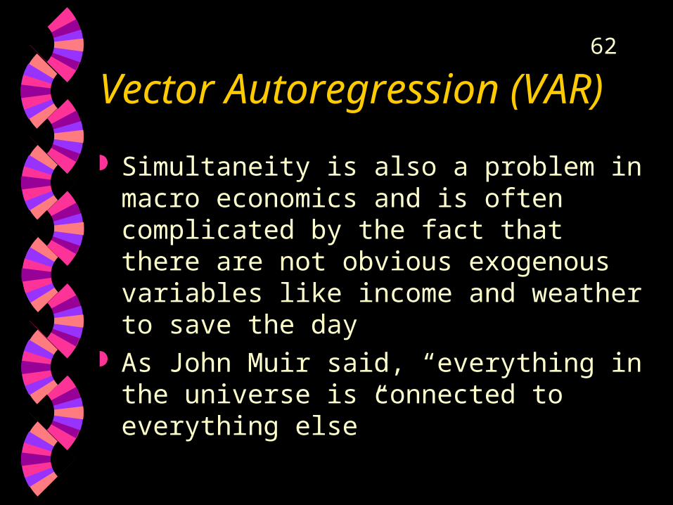
Vector Autoregression (VAR)

Simultaneity is also a problem in macro economics and is often complicated by the fact that there are not obvious exogenous variables like income and weather to save the day

As John Muir said, “everything in the universe is connected to everything else”

63VAR One possibility is to take advantage of the

dependence of a macro variable on its own past and the past of other endogenous variables. That is the approach of VAR, similar to the specification of Granger Causality tests

One difficulty is identification, working back from the equations we estimate, unlike the demand and supply example above

We miss our equation specific exogenous variables, income and weather

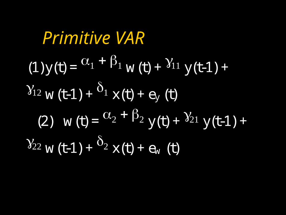
Primitive VAR

(1)y(t) = w(t) + y(t-1) +

w(t-1) + x(t) + ey(t)

(2) w(t) = y(t) + y(t-1) +

w(t-1) + x(t) + ew(t)

65

Standard VAR

Eliminate dependence of y(t) on contemporaneous w(t) by substituting for w(t) in equation (1) from its expression (RHS) in equation 2

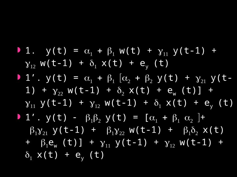
1. y(t) = w(t) + y(t-1) + w(t-1) + x(t) + ey(t)

1’. y(t) = y(t) + y(t-1) + w(t-1) + x(t) + ew(t)] + y(t-1) + w(t-1) + x(t) + ey(t)

1’. y(t) y(t) = [+ y(t-1) + w(t-1) + x(t) + ew(t)] + y(t-1) + w(t-1) + x(t) + ey(t)

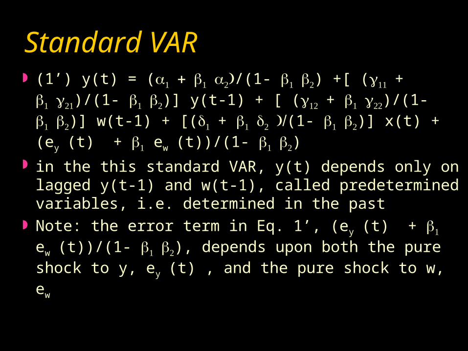
Standard VAR (1’) y(t) = (/(1- ) +[ (+

)/(1- )] y(t-1) + [ (+ )/(1- )] w(t-1) + [(+ (1- )] x(t) + (ey(t) + ew(t))/(1- )

in the this standard VAR, y(t) depends only on lagged y(t-1) and w(t-1), called predetermined variables, i.e. determined in the past

Note: the error term in Eq. 1’, (ey(t) + ew(t))/(1- ), depends upon both the pure shock to y, ey(t) , and the pure shock to w, ew

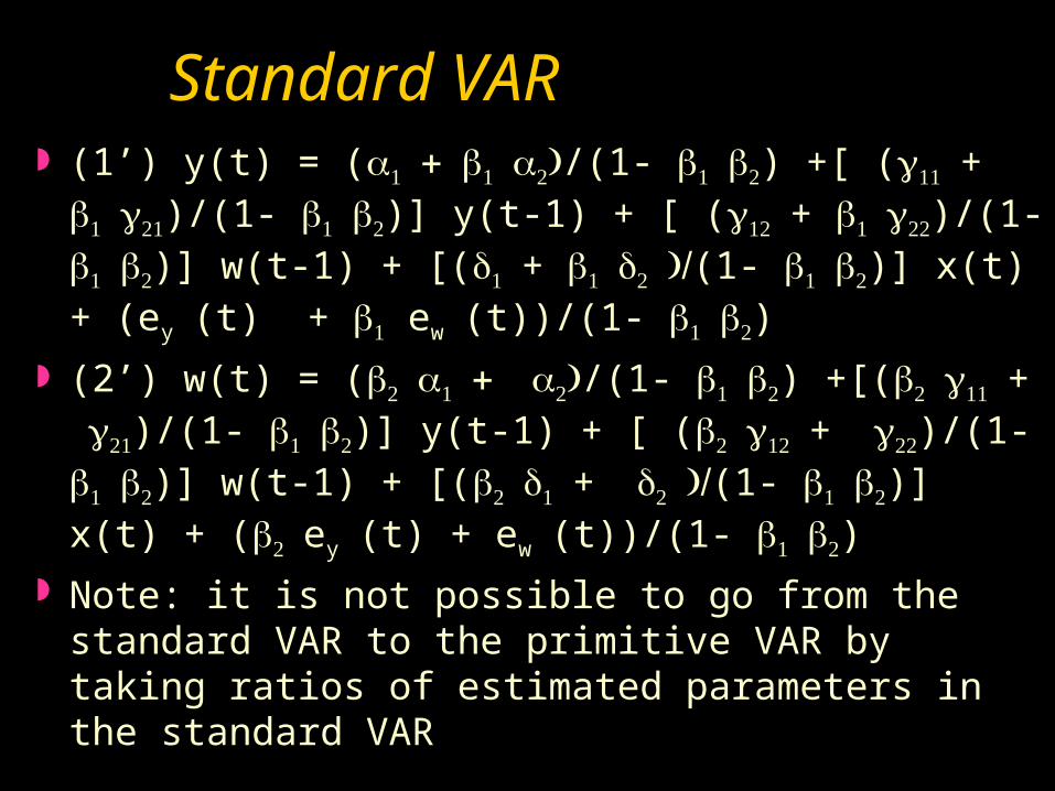
Standard VAR (1’) y(t) = (/(1- ) +[ (+ )/(1-

)] y(t-1) + [ (+ )/(1- )] w(t-1) + [(+ (1- )] x(t) + (ey(t) + ew(t))/(1- )

(2’) w(t) = (/(1- ) +[(+ )/(1- )] y(t-1) + [ (+ )/(1- )] w(t-1) + [(+ (1- )] x(t) + (ey(t) + ew(t))/(1- )

Note: it is not possible to go from the standard VAR to the primitive VAR by taking ratios of estimated parameters in the standard VAR