Econ 219B Psychology and Economics: Applications (Lecture 5)...Stefano DellaVigna Econ 219B: Applications (Lecture 5) February 20, 2019 21 / 105. Reference Dependence: Non-Bunching

Econ 219B

Psychology and Economics: Applications

(Lecture 5)

Stefano DellaVigna

February 20, 2019

Stefano DellaVigna Econ 219B: Applications (Lecture 5) February 20, 2019 1 / 105

Outline

1 Reference Dependence: Housing

2 Reference Dependence: Non-Bunching Papers

3 Reference Dependence: Labor Supply

4 Reference Dependence: Employment and Effort

5 Reference Dependence: Job Search


Reference Dependence: Housing

Section 1




Model

Housing case, formalize intuition.

Seller chooses price P at saleHigher Price P

lowers probability of sale p (P) (hence p′ (P) < 0)increases utility of sale U (P)

If no sale, utility is U < U (P) (for all relevant P)



Model

Maximization problem:

maxP

p(P)U (P) + (1− p (P))U

F.o.c. implies

MG = p(P∗)U ′ (P∗) = −p′(P∗)(U (P∗)− U) = MC

Interpretation: Marginal Gain of increasing price equals MarginalCost

S.o.c are

2p′(P∗)U ′ (P∗) + p(P∗)U ′′ (P∗) + p′′(P∗)(U (P∗)− U) < 0

Need p′′(P∗)(U (P∗)− U) < 0 or not too positive



Model

Reference-dependent preferences with reference price P0:

v (P |P0) =

{P + η(P − P0) if P ≥ P0;P + ηλ(P − P0) if P < P0,

Can write as

p(P)(1 + η) = −p′(P)(P + η(P − P0)− U) if P ≥ P0

p(P)(1 + ηλ) = −p′(P)(P + ηλ(P − P0)− U) if P < P0

Plot Effect on MG and MC of loss aversion

Compare P∗λ=1 (equilibrium with no loss aversion) and P∗λ>1

(equilibrium with loss aversion)



Cases

Case 1. Loss Aversion λ increase price (P∗λ=1 < P0)

Case 2. Loss Aversion λ induces bunching at P = P0

(P∗λ=1 < P0)



Cases

Case 3. Loss Aversion has no effect (P∗λ=1 > P0)

General predictions. When aggregate prices are low:

High prices P relative to fundamentalsBunching at purchase price P0

Lower probability of sale p (P), longer waiting on market


Reference Dependence: Housing Genesove & Mayer (2001)

Data

Genesove-Mayer (QJE, 2001)Evidence: Data on Boston Condominiums, 1990-1997

Substantial market fluctuations of price



Setup

Observe

Listing price Li ,t and last purchase price P0

Observed Characteristics of property Xi

Time Trend of prices δt

Define:

Pi ,t is market value of property i at time t

Ideal Specification:

Li ,t = Pi ,t + m1Pi,t<P0

(P0 − Pi ,t

)+ εi ,t

= βXi + δt + vi + mLoss∗ + εi ,t



Model

However:Do not observe Pi ,t , given vi (unobserved quality)Hence do not observe Loss∗

Two estimation strategies to bound estimates. Model 1:

Li ,t = βXi + δt + m1Pi,t<P0(P0 − βXi − δt) + εi ,t

This model overstate the loss for high unobservable homes(high vi )Bias upwards in m, since high unobservable homes should havehigh Li ,i

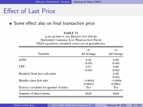
Model 2:

Li ,t = βXi+δt+α (P0 − βXi − δt)+m1Pi,t<P0(P0 − βXi − δt)+εi ,t

Estimates of impact on sale price





Effect of Experience

Effect of experience: Larger effect for owner-occupied



Effect of Last Price

Some effect also on final transaction price



Implications

Lowers the exit rate (lengthens time on the market)

Overall, plausible set of results that show impact of referencepoint


Reference Dependence: Housing Andersen et al. (2020)

Modern Evidence

Andersen, Badarinza, Liu, Marx, and Ramadorai (2020)

Administrative data set of house sales in Denmark for 1992-2016

217,028 listings

Compute ln(P) with hedonic model as above

Compute predicted gain ln(G ) = ln(P)− ln(P0)

Compute mortgage exposure ln(P)− ln(M)



Graphical Evidence

Figure 3Listing premia, gains, and home equity

Panel A reports binned average values (in 3% steps) for the listing premium (`) along both levels of

expected gains and home equity. Panel B shows the underlying binned values for two cross-sections: In

the left plot, we condition on a home equity level of 20%, and in the right plot on a level of expected

gains of 0%. We use these two representative cross-sections to generate the empirical moments used in

structural estimation.

Panel A: Listing premium surface

Home equity (%)

4020

020

40

Gains (%)

4020

020

40

Listing premium

(%)

0

10

20

30

40

50

G = 0%H = 20%

Panel B: Listing premia moments

-40 -20 0 20 40Gains (%)

0

5

10

15

20

25

30

35

40

Listin

g pr

emiu

m (%

)

-40 -20 0 20 40Home equity (%)

0

5

10

15

20

25

30

35

40Lis

ting

prem

ium

(%)

51

Page 58 of 117



Cost of Reference Dependence

Kink in slope consistent with reference dependence.Further: shape of kink in slope should depend on cost of kink–> The length of delay caused by a higher listing priceSeparate markets with higher and lower concave demand

Figure 4Listing premium-gain slope and demand concavity

Panel A shows the listing premium over gains (left-hand side) and demand concavity (right-hand side)

patterns. We sort municipalities by the estimated demand concavity, using municipalities in the top

and bottom 5% of observations. Demand concavity is estimated as the slope coefficient of the effect of

the listing premium on the probability of sale within six months, for ` ∈ [0, 50]. The slope of the listing

premium over gains is calculated for G < 0. For better illustration of the main effect, we adjust the

quantities measured to have the same level at G = 0% and ` = 0% respectively. The left-hand side of

Panel B shows the correlation between the estimated listing premium slope and demand concavity across

municipalities using a binned scatter plot with equal-sized bins. The right-hand side of Panel B shows a

binned scatter plot of the correlation between the main instrument, the share of listed apartments and

row houses in a given municipality, and demand concavity in a binned scatter plot with equal-sized bins.

Panel A

40 20 0 20 40Gains (%)

0

5

10

15

20

25

30

35

Listin

g pr

emiu

m (%

)(N

orm

alize

d fo

r G=0

%)

Strong demand concav. (top 5%)Weak demand concav. (bottom 5%)

10 0 10 20 30Listing premium (%)

0.2

0.3

0.4

0.5

0.6

0.7

0.8

Prob

. of s

ale

(Nor

mal

ized

for

=0%

)

Strong demand concav. (top 5%)Weak demand concav. (bottom 5%)

Panel B

1.2 1.0 0.8 0.6 0.4 0.2Demand concavity

0.7

0.6

0.5

0.4

0.3

Listin

g pr

emiu

m sl

ope

0.1 0.2 0.3 0.4 0.5 0.6 0.7 0.8Homogeneity

1.1

1.0

0.9

0.8

0.7

0.6

0.5

0.4

Dem

and

conc

avity

52

Page 59 of 117



Bunching

Also: Direct evidence on bunching

Figure 5Moments: bunching and extensive margin

Panel A reports the frequency of observed transactions in terms of potential gains (left-hand side plot)

and realized gains (right-hand side plot). This serves as the basis for the estimation of bunching, which

we use as an empirical moment in our structural estimation exercise. Panel B reports the likelihood of

listing with respect to potential gains. We calculate this by calculating the observed number of listings

relative to the total stock of properties with potential gains in a given bin.

Panel A

-40 -30 -20 -10 0 10 20 30 40Gains (%)

0

1

2

3

4

5

6

Freq

uenc

y of

sale

s (%

)

-40 -30 -20 -10 0 10 20 30 40Realized gains (%)

0

1

2

3

4

5

6Fr

eque

ncy

of sa

les (

%)

Bunchingaround 0%

Panel B

-40 -20 0 20 40Gains (%)

0

1

2

3

4

5

6

7

Listin

g pr

obab

ility

(%)

-40 -20 0 20 40Home equity (%)

0

1

2

3

4

5

6

7

Listin

g pr

obab

ility

(%)

53

Page 60 of 117

Cleaner evidence of reference dependence in housing listings


Reference Dependence: Non-Bunching

Section 2




Previous Papers: Bunching Assumption

Previous papers had bunching implication

Some papers test for bunching (mergers, tax evasion, marathonrunning)Some papers do not test it... but should! (housing)

For bunching test, need

Reference point r obvious enough to people AND researcher(house purchase price, zero taxes, round number goal)Effort can be altered to get to reference point



Next Set of Papers: No Bunching

Next set of papers, these conditions do not apply:

Choice is still about effort BUTReference point r not an exact number (labor supply, effort andcrime, job search)

Identification in these papers typically relies on variants of:

Loss aversion induces higher marginal utility of income to left ofreference pointIdentify comparing when to the left of reference point, versus tothe rightStill need some model about reference point (more later on this)


Reference Dependence: Labor Supply

Section 3




Framework

Does reference dependence affect work/leisure decision?

Framework:

effort h (no. of hours)hourly wage wReturns of effort: Y = w ∗ hLinear utility U (Y ) = YCost of effort c (h) = θh2/2 convex within a day

Standard model: Agents maximize

U (Y )− c (h) = wh − θh2

2



Framework

(Assumption that each day is orthogonal to other days – seebelow)

Reference dependence: Threshold T of earnings agent wants toachieve

Loss aversion for outcomes below threshold:

U =

{wh + η (wh − T ) if wh ≥ Twh + ηλ (wh − T ) if wh < T

with λ > 1 loss aversion coefficient

Reference-dependent agent maximizes

wh + η (wh − T )− θh2

2if h ≥ T/w

wh + ηλ (wh − T )− θh2

2if h < T/w



Framework

Derivative with respect to h:

(1 + η)w − θh if h ≥ T/w(1 + ηλ)w − θh if h < T/w

1 Case 1 ((1 + ηλ)w − θT/w < 0).

Optimum at h∗ = (1 + ηλ)w/θ < T/w



Framework

2 Case 2 ((1 + ηλ)w − θT/w > 0 > (1 + η)w − θT/w)

Optimum at h∗ = T/w

3 Case 3 ((1 + η)w − θT/w > 0)

Optimum at h∗ = (1 + η)w/θ > T/w



Standard theory (λ = 1)

Interior maximum: h∗ = (1 + η)w/θ (Cases 1 or 3)

Labor supply

Combine with labor demand: h∗ = a − bw , with a > 0, b > 0.



Model with reference dependence (λ > 1)

Case 1 or 3 still existBUT: Case 2. Kink at h∗ = T/w for λ > 1Combine Labor supply with labor demand: h∗ = a − bw , witha > 0, b > 0.

Case 2: On low-demand days (low w) need to work harder toachieve reference point T � Work harder � Opposite tostandard theoryStefano DellaVigna Econ 219B: Applications (Lecture 5) February 20, 2019 29 / 105

Reference Dependence: Labor Supply Camerer et al. (1997)

Camerer, Babcock, Loewenstein, and Thaler (QJE

1997)

Data on daily labor supply of New York City cab drivers

70 Trip sheets, 13 drivers (TRIP data)1044 summaries of trip sheets, 484 drivers, dates: 10/29-11/5,1990 (TLC1)712 summaries of trip sheets, 11/1-11/3, 1988 (TLC2)

Notice data feature: Many drivers, few days in sample



Framework

Analysis in paper neglects wealth effects: Higher wage today �Higher lifetime income

Justification:

Correlation of wages across days close to zeroEach day can be considered in isolation�Wealth effects of wage changes are very small

Test:

Assume variation across days driven by ∆a (labor demandshifter)Do hours worked h and w co-vary positively (standard model)or negatively?



Raw evidence



Model

Estimate:

log (hi ,t) = α + β log (Yi ,t/hi ,t) + Xi ,tΓ + εi ,t .

Estimates of β:

β = −.186 (s.e. 129) – TRIP with driver f.e.

β = −.618 (s.e. .051) – TLC1 with driver f.e.β = −.355 (s.e. .051) – TLC2

Estimate is not consistent with prediction of standard model

Indirect support for income targeting



Economic Issue 1

Reference-dependent model does not predict (log-) linear,negative relation

What happens if reference income is stochastic? (Koszegi-Rabin,2006)



Econometric Issue 1

Division bias in regressing hours on log wages

Wages are not directly observed – Computed at Yi ,t/hi ,t

Assume hi ,t measured with noise: hi ,t = hi ,t ∗ φi ,t . Then,

log(hi ,t

)= α + β log

(Yi ,t/hi ,t

)+ εi ,t .

becomes

log (hi ,t)+log (φi ,t) = α+β [log(Yi ,t)− log(hi ,t)]−β log(φi ,t)+εi ,t .

Downward bias in estimate of β

Response: instrument wage using other workers’ wage on sameday



Econometric Issue 1: Use IV

IV Estimates:

Notice: First stage not very strong (and few days in sample)



Econometric issue 2

Are the authors really capturing demand shocks or supplyshocks?

Assume θ (disutility of effort) varies across days.

Even in standard model we expect negative correlation of hi ,tand wi ,t

Camerer et al. argue for plausibility of shocks due to a ratherthan θStefano DellaVigna Econ 219B: Applications (Lecture 5) February 20, 2019 37 / 105

Reference Dependence: Labor Supply Farber (2005)

Farber (JPE, 2005)

Re-Estimate Labor Supply of Cab Drivers on new data

Address Econometric Issue 1 (Division Bias)

Data:

244 trip sheets, 13 drivers, 6/1999-5/2000349 trip sheets, 10 drivers, 6/2000-5/2001Daily summary not available (unlike in Camerer et al.)Notice: Few drivers, many days in sample



Model

Key specification: Hazard model that does not suffer fromdivision bias

Dependent variable is dummy Stopi ,t = 1 if driver i stops athour t:

Stopi ,t = Φ (α + βYYi ,t + βhhi ,t + ΓXi ,t)

Control for hours worked so far (hi ,t) and other controls Xi ,t

Does a higher earned income Yi ,t increase probability of stopping(β > 0)?



Results

Positive, but not significant effect of Yi ,t on probability ofstopping:

10 percent increase in Y ($15) � 1.6 percent increase instopping prob. (.225 pctg. pts. increase in stopping prob. outof average 14 pctg. pts.) � 0.16 elasticityCannot reject large effect: 10 pct. increase in Y increasestopping prob. by 6 percent � 0.6 elasticity

Qualitatively consistent with income targeting

Also notice:

Failure to reject standard model is not the same as rejectingalternative model (reference dependence)Alternative model is not spelled out


Reference Dependence: Labor Supply Fehr and Goette (2007)

Still, Supply or Demand?

Farber (2005) cannot address the Econometric Issue 2: Is itSupply or Demand that Varies

Fehr and Goette (AER 2007). Experiments on BikeMessengers

Use explicit randomization to deal with Econometric Issues 1and 2

Combination of:

Experiment 1. Field Experiment shifting wage andExperiment 2. Lab Experiment (relate to evidence on lossaversion)...... on the same subjects

Slides courtesy of Lorenz Goette


5

The Experimental Setup in this Study

Bicycle Messengers in Zurich, Switzerland Data: Delivery records of Veloblitz and Flash Delivery

Services, 1999 - 2000. Contains large number of details on every package

delivered.

Observe hours (shifts) and effort (revenues pershift).

Work at the messenger service Messengers are paid a commission rate w of their

revenues rit. (w = „wage“). Earnings writ

Messengers can freely choose the number of shiftsand whether they want to do a delivery, whenoffered by the dispatcher.

suitable setting to test for intertemporalsubstitution.

Highly volatile earnings Demand varies strongly between days

Familiar with changes in intertemporal incentives.

6

Experiment 1

The Temporary Wage Increase Messengers were randomly assigned to one of two

treatment groups, A or B. N=22 messengers in each group

Commission rate w was increased by 25 percentduring four weeks Group A: September 2000

(Control Group: B) Group B: November 2000

(Control Group: A)

Intertemporal Substitution Wage increase has no (or tiny) income effect. Prediction with time-separable prefernces, t= a day:

Work more shifts Work harder to obtain higher revenues

Comparison between TG and CG during theexperiment. Comparison of TG over time confuses two

effects.

7

Results for Hours

Treatment group works 12 shifts, Control Groupworks 9 shifts during the four weeks.

Treatment Group works significantly more shifts (X2(1)= 4.57, p<0.05)

Implied Elasticity: 0.8

-Ln[

-Ln(

Sur

viva

l Pro

babi

litie

s)]

Hor

izon

tal D

iffer

ence

= %

cha

nge

in h

azar

d

Figure 6: The Working Hazard during the Experimentln(days since last shifts) - experimental subjects only

Wage = normal level Wage = 25 Percent higher

0 2 4 6

-2

-1

0

1

8

Results for Effort: Revenues per shift

Treatment Group has lower revenues than ControlGroup: - 6 percent. (t = 2.338, p < 0.05)

Implied negative Elasticity: -0.25

Distributions are significantly different(KS test; p < 0.05);

The Distribution of Revenues during the Field Experiment

0

0.05

0.1

0.15

0.2

60 140 220 300 380 460 540

CHF/shift

Fre

quency

TreatmentGroup

Control Group

9

Results for Effort, cont.

Important caveat Do lower revenues relative to control group reflect

lower effort or something else?

Potential Problem: Selectivity Example: Experiment induces TG to work on bad days.

More generally: Experiment induces TG to work ondays with unfavorable states If unfavorable states raise marginal disutility of

work, TG may have lower revenues during fieldexperiment than CG.

Correction for Selectivity Observables that affect marginal disutility of work.

Conditioning on experience profile, messengerfixed effects, daily fixed effects, dummies forprevious work leave result unchanged.

Unobservables that affect marginal disutility of work? Implies that reduction in revenues only stems

from sign-up shifts in addition to fixed shifts. Significantly lower revenues on fixed shifts, not

even different from sign-up shifts.

11

Measuring Loss Aversion

A potential explanation for the results Messengers have a daily income target in mind They are loss averse around it Wage increase makes it easier to reach income target

That‘s why they put in less effort per shift

Experiment 2: Measuring Loss Aversion Lottery A: Win CHF 8, lose CHF 5 with probability 0.5.

46 % accept the lottery

Lottery C: Win CHF 5, lose zero with probability 0.5;or take CHF 2 for sure 72 % accept the lottery

Large Literature: Rejection is related to loss aversion.

Exploit individual differences in Loss Aversion

Behavior in lotteries used as proxy for loss aversion. Does the proxy predict reduction in effort during

experimental wage increase?

12

Measuring Loss Aversion

Does measure of Loss Aversion predictreduction in effort?

Strongly loss averse messengers reduce effortsubstantially: Revenues are 11 % lower (s.e.: 3 %)

Weakly loss averse messenger do not reduce effortnoticeably: Revenues are 4 % lower (s.e. 8 %).

No difference in the number of shifts worked.

Strongly loss averse messengers put in lesseffort while on higher commission rate

Supports model with daily income target

Others kept working at normal pace,consistent with standard economic model

Shows that not everybody is prone to this judgmentbias (but many are)

Reference Dependence: Labor Supply Other Work

Farber (2008)

Farber (AER 2008) goes beyond Farber (JPE, 2005) andattempts to estimate model of labor supply with loss-aversion

Estimate loss-aversion δEstimate (stochastic) reference point T

Same data as Farber (2005)

Results:

significant loss aversion δhowever, large variation in T mitigates effect of loss-aversion



Farber (2008)

δ is loss-aversion parameter

Reference point: mean θ and variance σ2



Crawford and Meng (AER 2011)

Re-estimates on Farber (2005) data allowing for two dimensionsof reference dependence:

Hours (loss if work more hours than h)Income (loss if earn less than Y )

Re-estimates Farber (2005) data for:

Wage above average (income likely to bind)Wages below average (hours likely to bind)

Perhaps, reconciling Camerer et al. (1997) and Farber (2005)

w > w e : hours binding � hours explain stoppingw < w e : income binding � income explains stopping



Crawford and Meng (2011)


Reference Dependence: Labor Supply Last Three Years

Farber (QJE 2015)

Finally data set with large K and large T

K = 62, 000 driversT = 5 ∗ 365 (2009 to 2013)100+ million trips!Electronic record of all information (except tips)

Inexplicably, most of analysis uses discredited OLS specification

We focus on hazard model (Table 7) as in Farber (2005)

P(stopping) for $300-$349 compared to $200-$224 is0.059− 0.015 = 0.044 higher out of average of 0.14Thus, 31% increase in stopping for a 51% increase in income–> elasticity of 0.6!Within the confidence interval of Farber (2005) and clearlysizable



Farber (2015)

dependence, and perhaps income targeting, is important, sur-vival probabilities at given hours should be lower due to theincome shock. Without income reference dependence (or impor-tant daily income effects), survival probabilities should be unaf-fected by the income shock.

Figure III contains separate plots for day and night shifts ofthe effect on shift survival of the 20 percent uniform incomeshock. This shows a small reduction in the survival probabilitythroughout day shifts (about 2.4 percentage points by 12 hours)and virtually no reduction (0.4 percentage points by 12 hours) onnight shifts.

In the second counterfactual, I shock hours by increasing theobserved time on and between each trip by 20 percent (holdingfare income constant). I then recalculate accumulated hours andcompare the predicted survival probability by income category

TABLE VII

MARGINAL EFFECTS OF INCOME AND HOURS ON PROBABILITY OF ENDING SHIFT (LINEAR

PROBABILITY MODEL)

(1) (2) (3) (4)Income ($) Day shift Night shift Hours Day shift Night shift

100–149 0.0001 !0.0045 3–5 0.0020 !0.0049(0.0003) (0.0003) (0.0004) (0.0003)

150–199 0.0044 !0.0077 6 0.0001 0.0007(0.0006) (0.0005) (0.0007) (0.0006)

200–224 0.0157 !0.0062 7 0.0034 0.0223(0.0010) (0.0007) (0.0011) (0.0010)

225–249 0.0264 !0.0046 8 0.0281 0.0536(0.0013) (0.0008) (0.0017) (0.0016)

250–274 0.0389 !0.0042 9 0.0750 0.0897(0.0017) (0.0011) (0.0025) (0.0022)

275–299 0.0506 !0.0033 10 0.1210 0.1603(0.0020) (0.0013) (0.0035) (0.0031)

300–349 0.0596 !0.0027 11 0.1236 0.2563(0.0024) (0.0017) (0.0050) (0.0051)

350–399 0.0607 0.0011 12 0.1004 0.2573(0.0028) (0.0024) (0.0078) (0.0142)

" 400 0.0702 0.0101 " 13 0.1093 0.2406(0.0034) (0.0035) (0.0050) (0.0063)

Notes. Based on estimates of two linear probability models for the probability of stopping: day shifts(columns (1) and (3)) and night shifts (columns (2) and (4)). The base category for income is $0–99 and thebase category for hours is 0–2. Both models additionally include sets of fixed effects for driver, hour of theday by day of the week (168), week of the year (52), and year (5) as well as indicators for the periodsubsequent to the September 4, 2012, fare increase and major holiday. Robust standard errors clusteredby driver are in parentheses. See text for information on sample size and composition.

QUARTERLY JOURNAL OF ECONOMICS2006

Downloaded from https://academic.oup.com/qje/article-abstract/130/4/1975/1916077/Why-you-Can-t-Find-a-Taxi-in-the-Rain-and-Otherby UNIVERSITY OF CALIFORNIA, Berkeley useron 04 September 2017



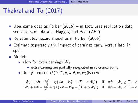
Thakral and To (2017)

Uses same data as Farber (2015) – in fact, uses replication dataset, also same data as Haggag and Paci (AEJ)

Re-estimates hazard model as in Farber (2005)

Estimate separately the impact of earnings early, versus late, inspell

Model:allow for extra earnings W0

extra earning are partially integrated in reference point

Utility function U (h;T , η, λ, θ,w ,w0)is now

W0 + wh − θh2

2 + η (wh + W0 − (T + αW0)) if wh + W0 ≥ T + αW0

W0 + wh − θh2

2 + ηλ (wh + W0 − (T + αW0)) if wh + W0 < T + αW0




Special case 1: Reference point fully reflects extra earnings(α = 1):

W0 cancels out from expression above –> no effectIntuition: extra income already expected, no impact ongain/loss

Special case 2: Reference point not affected by extra earnings(α = 0):

In this case can rewrite solution above replace T with T −W0

5

10

15

20

5 10 15 20

w

h

W0

0

50




Table 3: Stopping model estimates: Income e�ect at 8.5 hours—Subsamples

(1) (2) (3)Night weekday Medallion owners Top decile experience

Panel AIncome e�ect 0.3564 0.5421 0.4625

(0.0473) (0.1548) (0.0805)Panel BIncome in hour 2 0.0725 -0.1175 -0.0130

(0.0742) (0.2351) (0.1236)Income in hour 4 0.0077 0.0282 0.3062

(0.0717) (0.2269) (0.1284)Income in hour 6 0.2645 0.2363 0.3309

(0.0732) (0.2389) (0.1267)Income in hour 8 0.3270 0.5714 0.5580

(0.0752) (0.2246) (0.1335)Note: Panel A reports estimates from Equation (1) of the percentage-point increase in theprobability of ending a shift at 8.5 hours when cumulative earnings is 10 percent higher. Panel Breports estimates from Equation (2) of the percentage-point change in the probability of endinga shift at 8.5 hours in response to a $10 increase in earnings accumulated at di�erent timesin the shift. The columns correspond to di�erent sample restrictions: (1) trips on Friday andSaturday after 5 pm, (2) cabdrivers who operate exactly one cab and no other driver shares thatcab, and (3) the latest 10 percent of shifts for drivers with over 100 shifts. The control variablesconsist of the full set from Table 2. Standard errors reported in parentheses are adjusted forclustering at the driver level.

71

Estimates in Panel B areincreases in pp in P(stop) for $10 4Y in that hour, equal to5% higher income overallMean stopping probability is 13.6%

$10 4Y in hour 2 –> 4P(stop) = 0.07% –> ηStop,Y = 0.1

$10 4Y in hour 8 –> 4P(stop) = 0.32% –> ηStop,Y = 0.46




Findings provide evidence on speed of formation of referencepoint:

Income earned early during the day is already incorporated intoreference point T –> Does not impact stopping

Income earned late in the shift not incorporated –> Affectstopping

Provides evidence of backward looking reference points

Can also be interpreted as forward-looking (KR) delayedexpectations


Reference Dependence: Employment and Effort

Section 4

Reference Dependence: Employment and

Effort


Reference Dependence: Employment and Effort Mas (2006)

Mas (2006): Police Performance

More on labor markets: Do reference points affect performance?

Mas (QJE 2006) examines police performance

Exploits quasi-random variation in pay due to arbitration

Background

60 days for negotiation of police contract � If undecided,arbitration9 percent of police labor contracts decided with final offerarbitration



Framework

pay is w · (1 + r)

union proposes ru, employer proposes re , arbitrator prefers ra

arbitrator chooses re if |re − ra| ≤ |ru − ra|P (re , ru) is probability that arbitrator chooses re

Distribution of ra is common knowledge (cdf F )

Assume re ≤ ra ≤ ru � Then

P = P (ra − re ≤ ru − ra) = P (ra ≤ (ru + re) /2) = F (ru + re

2)



Nash Equilibrium

If ra is certain, Hotelling game: convergence of re and ru to ra

Employer’s problem:

maxre

PU (w (1 + re)) + (1− P)U (w (1 + r ∗u ))

Notice: U ′ < 0

First order condition (assume ru ≥ re):

P ′

2[U (w (1 + r ∗e ))− U (w (1 + r ∗u ))] + PU ′ (w (1 + r ∗e ))w = 0

r ∗e = r ∗u cannot be solution � Lower re and increase utility(U ′ < 0)



Union’s problem

Maximize:

maxru

PV (w (1 + r ∗e )) + (1− P)V (w (1 + ru))

Notice: V ′ > 0

First order condition for union:

P ′

2[V (w (1 + r∗e ))− V (w (1 + r∗u ))] + (1− P)V ′ (w (1 + r∗u ))w = 0

To simplify, assume U (x) = −bx and V (x) = bx

This implies V (w (1 + r ∗e ))− V (w (1 + r ∗u )) =−U (w (1 + r ∗e ))− U (w (1 + r ∗u )), so

−bP∗w = − (1− P∗) bw

Result: P∗ = 1/2



Prediction

Prediction (i) in Mas (2006): “If disputing parties are equallyrisk-averse, the winner in arbitration is determined by a cointoss.”

Therefore, as-if random assignment of winner

Use to study impact of pay on police effort

Data:

383 arbitration cases in New Jersey, 1978-1995Observe offers submitted re , ru, and ruling raMatch to UCR crime clearance data (=number of crimes solvedby arrest)



Summary Statistics

Compare summary statistics of cases when employer and when police wins

Estimated P = .344 6= 1/2 � Unions more risk-averse than employers

No systematic difference between Union and Employer cases except for re



Effects on Performance

Graphical evidence of effect of ruling on crime clearance rate

Significant effect on clearance rate for one year after ruling

Estimate of the cumulated difference between Employer andUnion cities on clearance rates and crime



Effects on Performance

Union win –> 15 more clearances out of 100,000 each month



Do reference points matter?

Plot impact on clearances rates (12,-12) as a function ofra − (re + ru)/2



Effect of loss is larger than effect of gain



Reference Dependence Model

Column (3): Effect of a gain relative to (re + ru)/2 is notsignificant; effect of a loss is

Columns (5) and (6): Predict expected award ra usingcovariates, then compute ra − ra

ra − ra does not matter if union winsra − ra matters a lot if union loses

Assume policeman maximizes

maxe

[U + U (w)

]e − θe

2

2

where

U (w) =

{w + η(w − w) if w ≥ ww + ηλ (w − w) if w < w



Reference Dependence Model

Reduced form of reciprocity model where altruism towards thecity is a function of how nice the city was to the policemen(U + U (w))

F.o.c.:U + U (w)− θe = 0

Then

e∗ (w) =U

θ+

1

θU (w)

It implies that we would estimate

Clearances = α + β (ra − ra) + γ (ra − ra) 1 (ra − ra < 0) + ε

with β > 0 (also in standard model) and γ > 0 (not in standardmodel)



Results

Compare to observed pattern

Close to predictions of model


Reference Dependence: Job Search

Section 5

Reference Dependence: Job Search


Reference Dependence: Job Search DellaVigna et al. (2017)

DellaVigna, Lindner, Reizer, Schmieder (QJE 2017)

Job Search in Hungary

Example where identification is not from comparing gains fromlosses

Identification comes from

how much at a loss relative to reference pointreference point adapts over timeaim to identify reference point adaptation


Introduction

Introduction

Large literature on understanding path of hazard rate fromunemployment with different models.Typical finding: There is a spike in the hazard rate at theexhaustion point of unemployment benefits.

⇒ Such a spike is not easily explained in the standard (McCall /Mortensen) model of job search.

⇒ To explain this path, one needs unobserved heterogeneity of aspecial kind, and/or storeable offers

Reference-Dependent Job Search 2 / 34

Introduction

Germany - Spike in Exit Hazard0

.02

.04

.06

.08

.1.1

2.1

4

0 5 10 15 20 25Duration in Months

12 Months Potential UI Duration 18 Months Potential UI Duration

AllHazard − Slopes differing on each side of Discontinuity

Source: Schmieder, von Wachter, Bender (2012)Reference-Dependent Job Search 3 / 34

Introduction

Simulation of Standard model

0 2 4 6 8 10 12 14 16 180

0.01

0.02

0.03

0.04

0.05

0.06

0.07

0.08

Period (months)

Haza

rdRate

Hazard Rate, Standard

Predicted path of the hazard rate for a standard model withexpiration of benefit at period 25


Model

Model - Set-up

We integrate reference dependence into standard McCall /Mortensen discrete time model of job searchJob Search:

Search intensity comes at per-period cost of c(st), which isincreasing and convexWith probability st , a job is found with salary wOnce an individual finds a job the job is kept forever

Optimal consumption-savings choice

Individuals choose optimal consumption ct (hand-to-mouthct = yt as special case)

Individuals are forward looking and have rational expectations


Model

Utility Function

Utility function v(c)

Flow utility ut(ct |rt) depends on reference point rt :

ut(ct |rt) ={

v(ct) + η(v(ct)− v(rt)) if ct ≥ rtv(ct) + ηλ(v(ct)− v(rt)) if ct < rt

η is weight on gain-loss utilityλ indicates loss aversionStandard model is nested for η = 0

Builds on Kahneman and Tversky (1979) and Kőszegi and Rabin(2006)

Note: No probability weighting or diminishing sensitivity


Model

Reference Point

Unlike in Kőszegi and Rabin (2006), but like in Bowman,Minehart, and Rabin (1999), reference point isbackward-lookingThe reference point in period t is the average income earnedover the N periods preceding period t and the period tincome:

rt =1

N + 1

t∑

k=t−Nyk


Model

Key Equations

An unemployed worker’s value function is

V Ut (At) = max

st∈[0,1];At+1u (ct |rt)−c (st)+δ

[stV

Et+1(At+1) + (1− st)V

Ut+1(At+1)

]

Value function when employed:

V Et+1(At+1) = max

ct+1u (ct+1|rt+1) + δV E

t+2(At+2).

Solution for optimal search:

c ′ (s∗t ) = δ[V Et+1 (At+1)− V U

t+1 (At+1)]

Solve for s∗t and c∗t using backward induction


Model

How does the model work?

Consider a step-wise benefit schedule

T T+N50

100

150

200

250

300

350

400

450

Periods

Ben

efit

Leve

l

Benefit

What are the predictions of the standard vs.reference-depedent model without heterogeneity?


Model

Example: Hazards under Two Models

T T+N50

100

150

200

250

300

350

400

450

Periods

Ben

efit

Leve

l

Benefit

Hazard Rate, Standard Model Hazard Rate, Ref.-Dep. Model

T T+N0

0.01

0.02

0.03

0.04

0.05

0.06

0.07

0.08Hazard rate in the Standard Model

Haz

ard

Rat

e

Periods


Model


T T+N50

100

150

200

250

300

350

400

450

Periods

Ben

efit

Leve

l

Benefit


T T+N0

0.01

0.02

0.03

0.04

0.05

0.06

0.07


Haz

ard

Rat

e

PeriodsT T+N

0

0.01

0.02

0.03

0.04

0.05

0.06

0.07

0.08Hazard rate in the Reference Dep. Model

Haz

ard

Rat

e

Periods


Model


Consider the introduction of an additional step-down after T1

periods, such that total benefits paid until T are identical:

T1 T T+N0

50

100

150

200

250

300

350

400

450

Periods

Ben

efit

Leve

l

Benefit

What are the predictions of the standard vs. ref.-dep. model?


Model


T1 T T+N0

50

100

150

200

250

300

350

400

450

Periods

Ben

efit

Leve

l

Benefit


T1 T T+N0

0.01

0.02

0.03

0.04

0.05

0.06

0.07


Haz

ard

Rat

e

PeriodsT1 T T+N

0

0.01

0.02

0.03

0.04

0.05

0.06

0.07


Haz

ard

Rat

e

Periods


Evidence from Hungary UI Benefits in Hungary

Benefit schedule before and after the reform

270 90

$342

$222

$171

$114

360

Mon

thly

UI B

enef

it

Number of days since UI claim 180

1st tier (UI) 2nd tier (UA)

Social Assistance (HH income dependent)

44,460

68,400

34,200

22,800

Before Nov, 2005 schedule

After Nov, 2005 schedule

Note: Eligible for 270 days in the first tier, base salary is higher than114,000HUF ($570), younger than 50.→ Benefit-Schedule Macro Context Institutional Context


Evidence from Hungary UI Benefits in Hungary

Define before and after


Evidence from Hungary Reduced Form Results

Hazard rates before and after0

.01

.02

.03

.04

.05

.06

.07

.08

0 200 400 600Number of days since UI claim

before afterSamplesize: 11867

Hazard by Duration

Survival Rate Reemployment Wages


Evidence from Hungary Reduced Form Results

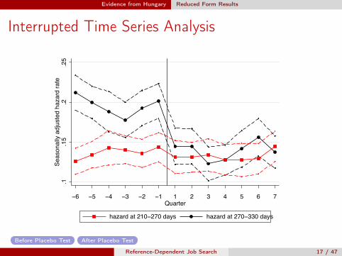
Interrupted Time Series Analysis

.1.1

5.2

.25

Sea

sona

lly a

djus

ted

haza

rd r

ate

−6 −5 −4 −3 −2 −1 1 2 3 4 5 6 7Quarter

hazard at 210−270 days hazard at 270−330 days

Before Placebo Test After Placebo Test


Model Estimation Estimation Method

Structural Estimation

We estimate model using minimum distance estimator:

minξ

(m (ξ)− m)′W (m (ξ)− m)

m - Empirical Moments (without controls)

35 15-day pre-reform hazard rates35 15-day pre-reform hazard rates

W is the inverse of diagonal of variance-covariance matrixFurther assumptions about utility maximization:

Log utility: v(c) = log(c)Assets A0 = 0, Borrowing limit L = 0, Interest rate R = 1Cost of effort c(s) = kj

s1+γ

1+γ


Model Estimation Estimation Method

Estimation Method

Parameters ξ to estimate:

λ loss component in utility functionN speed of adjustment of reference point15-day discount factor δ (fixed at δ = 0.995 for hand-to-mouthcase)Cost of effort curvature γUnobserved Heterogeneity: kh, km and kl cost types, and theirproportions (only one type for ref. dep. model)

Fixed parameters:Gain-loss utility weight η = 0 (standard model), η = 1 (ref.-dep.model) Link

Reemployment wage fixed at the empirical median Link

Start with hand-to-mouth estimates (ct = yt)


Model Estimation Hand-to-Mouth Estimates

Standard Model, 3 types (Hand-to-Mouth)

0 50 100 150 200 250 300 350 400 450 500 550Days elapsed since UI claimed

0

0.01

0.02

0.03

0.04

0.05

0.06

0.07

0.08

haza

rd r

ate

Hazard rates, actual and estimated

Actual Hazard, BeforeEstimated Hazard, BeforeActual Hazard, AfterEstimated Hazard, After


Model Estimation Hand-to-Mouth Estimates

Ref.-Dep. Model, 1 types (Hand-to-Mouth)


0

0.01

0.02

0.03

0.04

0.05

0.06

0.07

0.08

haza

rd r

ate




Model Estimation Estimates with Consumption-savings

Incorporating Consumption-Savings

Previous results have key weaknessReference-dependent workers are aware of painful loss utility atbenefit decreaseShould save in anticipationRuled out by hand-to-mouth assumption

Introduce optimal consumption:In each period t individuals choose search effort s∗t andconsumption c∗tEstimate also degree of patience δ and β, δ



Standard model (Optimal Consumption)

0 50 100 150 200 250 300 350 400 450 500 5500

0.01

0.02

0.03

0.04

0.05

0.06

0.07

0.08

Days elapsed since UI claimed

haza

rd r

ate



Standard model with 3 cost types and estimated δ performs nobetter than with hand-to-mouth assumption



Ref.-Dep. model (Optimal Consumption)


0

0.01

0.02

0.03

0.04

0.05

0.06

0.07

0.08

haza

rd r

ate



Reference-dependent model with estimated δ performs wellBUT: estimated δ = .9 (bi-weekly) – not realistic



Ref.-Dep. model - Discount Factor Estimated

Ref.-Dep. Model - β estimated Ref.-Dep. Model - δ estimated

0 50 100 150 200 250 300 350 400 450 500 5500

0.01

0.02

0.03

0.04

0.05

0.06

0.07

0.08

Days elapsed since UI claimed

haza

rd r

ate




0

0.01

0.02

0.03

0.04

0.05

0.06

0.07

0.08

haza

rd r

ate



The reference-dependent model with β, δ performs about equally well- Laibson (1997), O’Donoghue and Rabin (1999), Paserman (2008),Cockx, Ghirelli and van der Linden (2014)Estimated β = 0.58 with δ = .995, reasonableNoticed: maintained naiveté



Benchmark Estimates (Optimal Consumption)

Structural estimation of Standard and Ref.-Dep. models - Optimal Consumption(1) (2) (3) (4)

Standard RefD. Standard RefD.Discounting: Delta Delta Beta BetaParameters of Utility functionUtility function ν(.) log(b) log(b) log(b) log(b)Loss aversion λ 4.92 4.69

(0.58) (0.62)Gain utility η 1 1Adjustment speed of reference 184 167.5point N in days (11) (11.2)δ 0.93 0.89 0.995 0.995

(0.01) (0.02)1 1 0.92 0.58

β (0.01) (0.19)Parameters of Search Cost FunctionElasticity of search cost γ 0.4 0.81 0.07 0.4

(0.04) (0.16) (0.01) (0.2)Model FitGoodness of fit 227.5 194.0 229.0 183.5Number of cost-types 3 1 3 1



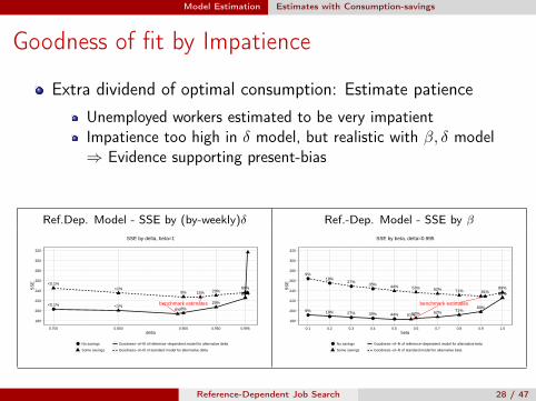
Goodness of fit by Impatience

Extra dividend of optimal consumption: Estimate patience

Unemployed workers estimated to be very impatientImpatience too high in δ model, but realistic with β, δ model⇒ Evidence supporting present-bias

Ref.Dep. Model - SSE by (by-weekly)δ Ref.-Dep. Model - SSE by β

●

benchmark estimates

<1%<0.1%

15%89%

29%8% 89%

<0.1% <1%8%

29%

89%

6%

180

200

220

240

260

280

300

320

0.700 0.800 0.900 0.950 0.995delta

SS

E

● No savings

Some savings

Goodness−of−fit of reference−dependent model for alternative delta

Goodness−of−fit of standard model for alternative delta

SSE by delta, beta=1

●●

●●

● ● ● ● ●

benchmark estimates

9%18%

27%35% 44% 53% 62% 71% 81%

89%

9% 18% 27% 35% 44% 53% 62% 71%80%

89%89%

51%

180

200

220

240

260

280

300

320

0.1 0.2 0.3 0.4 0.5 0.6 0.7 0.8 0.9 1.0beta

SS

E

● No savings

Some savings

Goodness−of−fit of reference−dependent model for alternative beta

Goodness−of−fit of standard model for alternative beta

SSE by beta, delta=0.995


Conclusion

Ongoing Work: Survey

Key prediction of different models on search effort

Search Effort, Standard model Search Effort, Reference Dependence

T T+N0

0.01

0.02

0.03

0.04

0.05

0.06

0.07


Haz

ard

Rat

e

PeriodsT T+N

0

0.01

0.02

0.03

0.04

0.05

0.06

0.07


Haz

ard

Rat

e

Periods

⇒ Ideally we would have individual level panel data on searcheffort


Conclusion


Build on Krueger and Mueller (2011, 2014):Large web based survey among UI recipients in NJ5% participation rateNo benefit expiration in their sample


Conclusion


Conduct SMS-based survey in 2017 in Germany with IABTwice-a-week ‘How many hours did you spend on search effortyesterday?’

Follow around 10,000 UI recipients over 4 months.Use discontinuity in benefit duration (6/8/10 months) to getcontrol groupExamine in particular search effort around benefit expiration

Advantages of SMS messages:

Very easy to reply / low cost to respondent.A lot of control, easy to send reminders etc.


Next Lecture

Section 6

Next Lecture


Next Lecture

Next Lecture

More Reference-Dependence:

InsuranceFinanceKR vs. backward looking ref. pointsEndowment EffectEffort


Documents

Econ 219B Psychology and Economics: Applications (Lecture 5)...Stefano DellaVigna Econ 219B: Applications (Lecture 5) February 20, 2019 21 / 105. Reference Dependence: Non-Bunching