ECOM 009 Macroeconomics 9 Lecture 9 - giuliofella.net

ECOM 009 Macroeconomics 9

Lecture 9

Giulio Fella

c� Giulio Fella, 2014 ECOM 009 Macroeconomics B - Lecture 9 232/256

Plan for this lecture

� Jorgensonian (neoclassical) theory of investment

� Tobin’s Q theory of investment

� The “neoclassical synthesis”: investment with convex

adjustment costs


The Jorgensonian neoclassical theory of investment

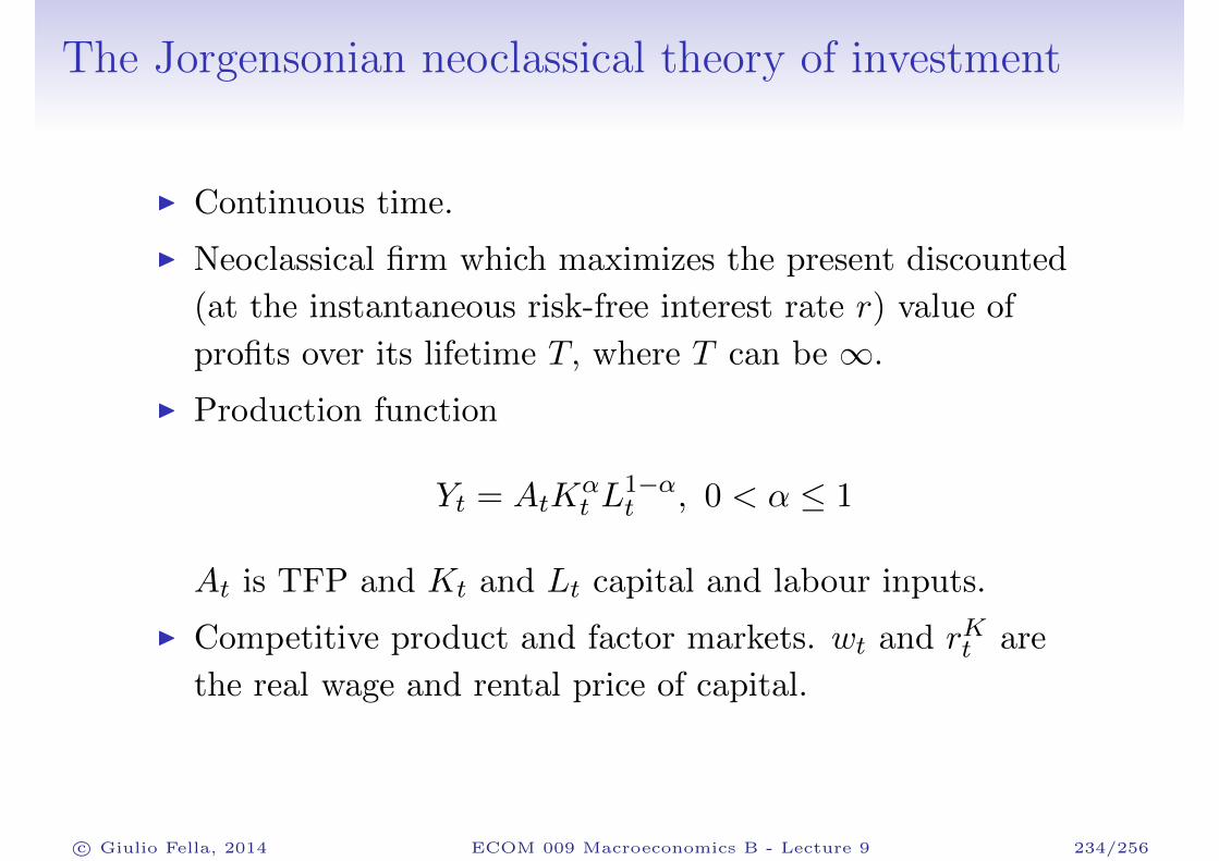
� Continuous time.

� Neoclassical firm which maximizes the present discounted

(at the instantaneous risk-free interest rate r) value of

profits over its lifetime T, where T can be ∞.

� Production function

Yt = AtKαt L

1−αt , 0 < α ≤ 1

At is TFP and Kt and Lt capital and labour inputs.

� Competitive product and factor markets. wt and rKt are

the real wage and rental price of capital.


Firm’s problem

� The firm’s optimization problem is

maxKt,Lt

V0 =

� ∞

0

�AtK

αt L

1−αt − wtLt − rKt Kt

�e−rtdt (154)

with FOCs

(1− α) (Kt/Lt)α = wt (155)

αAt (Kt/Lt)α−1 = rKt . (156)

� Given zero costs of adjusting labour and capital, the firm

chooses input quantities to equate the marginal product of

each factor to its rental cost period-by-period.


� Equation

αAt (Kt/Lt)α−1 = rKt .

embodies Jorgenson’s (1963) neoclassical theory of

investment.

� The return to one unit of capital invested in the firm is its

marginal product and at an optimum this must equal its

rental price.


What if capital is bought rather than rented?

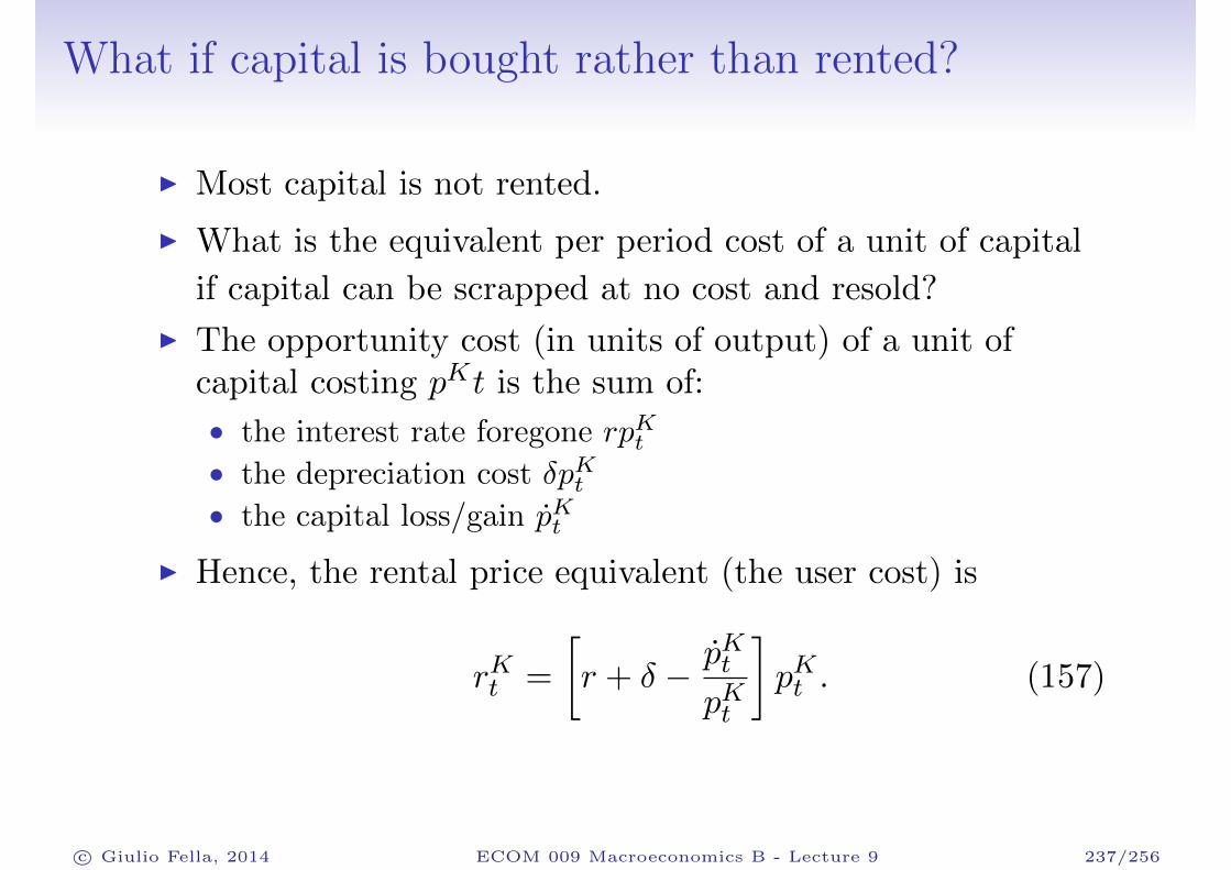
� Most capital is not rented.

� What is the equivalent per period cost of a unit of capital

if capital can be scrapped at no cost and resold?

� The opportunity cost (in units of output) of a unit ofcapital costing pKt is the sum of:

• the interest rate foregone rpKt• the depreciation cost δpKt• the capital loss/gain pKt

� Hence, the rental price equivalent (the user cost) is

rKt =

�r + δ − pKt

pKt

�pKt . (157)


Summarizing

For the Jorgensonian theory of investment:

1. The cost of capital depends on the instantaneous interest

rate. In general, the relevant interest rate is the one which

applies for the period over which capital can be adjusted;

2. It’s irrelevant whether the firm rents or owns its capital.1.

The firm should invest up to the point where the marginal

cost of capital equals its user cost.

3. Remembering that with Cobb-Douglas technology

MPK = αAPK, the optimal investment condition can be

written as

αYtKt

= rKt . (158)

1In fact, the user cost in (157) is the price at which the firm can rent

capital for one instant if the rental market for capital is competitive.c� Giulio Fella, 2014 ECOM 009 Macroeconomics B - Lecture 9 238/256

Implications (logical problems) of the theory I

The absence of adjustment costs implies that:

1. The firm does not have to look into the future. The future

is irrelevant for investment decisions → clearly

counterfactual.

2. The stock of capital Kt jumps discretely to keep the

marginal product of capital equal to its user cost → Gross

investment Kt → investment rate is zero in the absence of

shocks and +/- infinity otherwise.2.

3. The theory does not predict that investment is negatively

related to the user cost of capital. In fact it is not a theory

of investment but rather of the stock of capital

2This would improve only slightly if time were discrete. Firms would still

want to do all their adjustment immediately after a shock and be inactive

otherwise. The volatility of investment would still be counterfactually high.c� Giulio Fella, 2014 ECOM 009 Macroeconomics B - Lecture 9 239/256

Implications (logical problems) of the theory II

4. It is not even a theory of the capital stock Kt. Kt cannot

be determined separately from Lt or Yt (which are

undetermined under CRS). → theory of the optimal

capital/labour (or capital/output) ratio. Thus, it is a

theory of the optimal capital stock conditional on the level

of output.

5. The interest rate is assumed to be exogenous. What

happens in general equilibrium?


Early empirical tests

� Hall and Jorgenson (1967) sidestepped the problemassociated with 3. by assuming that

• output is predetermined when the firm chooses the stock of

capital

• the capital stock cannot adjust immediately to its frictionless

target in (158); e.g. ΔKt =n�

τ=0βτΔK∗

t−τ .

� This led to estimating an equation of the form

It − δKt =n�

τ=0βτΔK∗

t−τ (159)

Replacing in (159) gives

It − δKt =n�

τ=0

�βταΔ

Yt−τ

rKt−τ

�(160)


Findings

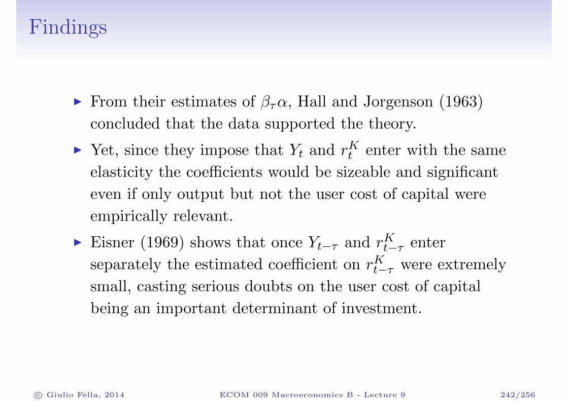
� From their estimates of βτα, Hall and Jorgenson (1963)

concluded that the data supported the theory.

� Yet, since they impose that Yt and rKt enter with the same

elasticity the coefficients would be sizeable and significant

even if only output but not the user cost of capital were

empirically relevant.

� Eisner (1969) shows that once Yt−τ and rKt−τ enter

separately the estimated coefficient on rKt−τ were extremely

small, casting serious doubts on the user cost of capital

being an important determinant of investment.


Remarks

� It has to be noted that the above formulation is not an

appropriate to test of the Jorgensonian theory of the

optimal capital stock alone.

� By imposing the short run adjustment dynamics (159) it

tests two hypotheses at the same time: the correctness of

the dynamics specification and the adequacy of the

Jorgensonian theory. This is a very important point to

understand its empirical failure.

� From a theoretical point of view, the estimating equation

(159) introduces adjustment costs implicitly without

having explicitly modelled them and derived their

theoretical implications.


Tobin’s q theory of investment

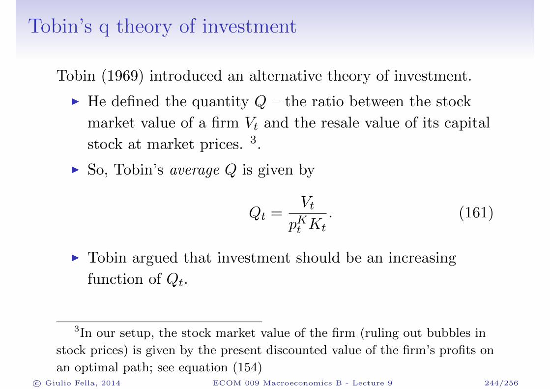
Tobin (1969) introduced an alternative theory of investment.

� He defined the quantity Q – the ratio between the stock

market value of a firm Vt and the resale value of its capital

stock at market prices. 3.

� So, Tobin’s average Q is given by

Qt =Vt

pKt Kt. (161)

� Tobin argued that investment should be an increasing

function of Qt.

3In our setup, the stock market value of the firm (ruling out bubbles in

stock prices) is given by the present discounted value of the firm’s profits on

an optimal path; see equation (154)c� Giulio Fella, 2014 ECOM 009 Macroeconomics B - Lecture 9 244/256

Empirical tests

� It is effectively a no-arbitrage argument. If Qt is below one,

a profit can be made by buying the firm on the stock

market at Vt, scrapping its capital and selling it at

pKt Kt > Vt. Viceversa, if Qt is larger than one.

� Unfortunately, as for the user cost of capital, the coefficient

on Qt in estimated investment equations turned out to be

disappointingly small.


The “neoclassical synthesis”

� In the early 80s researchers - namely Abel (1979) and

Hayashi (1982) - were able to unify these two strands of the

theory. The model they used encompasses Jorgenson’s

model by allowing for positive adjustment costs.

� This model (which was first introduced in the late 60s but

not linked to Tobin’s Q at the time) has the great

advantage of explicitly introducing adjustment costs in the

optimization problem.

� Rather than assuming that capital can be costlessly

installed and scrapped the model assumes convex costs of

investment and disinvestment e.g. C(It) = cI2t /2.


Implications

1. The existence of adjustment costs implies that expectations

are important. → When investing today the likelihood that

the investment decision has to be reversed tomorrow due to

a fall in productivity matters.

2. The convexity of the cost of investment implies that the

marginal investment cost (and the average unit cost) is

increasing in the size of investment/disinvestment. So, it is

optimal to spread investment over time.


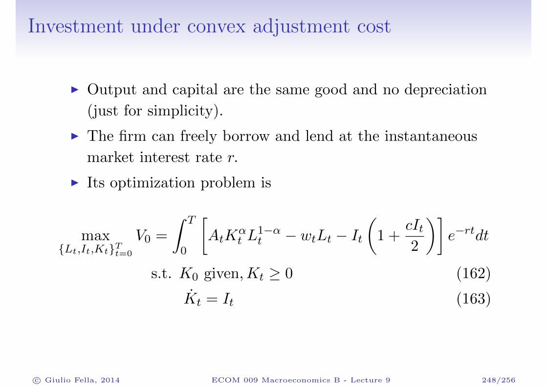
Investment under convex adjustment cost

� Output and capital are the same good and no depreciation

(just for simplicity).

� The firm can freely borrow and lend at the instantaneous

market interest rate r.

� Its optimization problem is

max{Lt,It,Kt}Tt=0

V0 =

� T

0

�AtK

αt L

1−αt − wtLt − It

�1 +

cIt2

��e−rtdt

s.t. K0 given, Kt ≥ 0 (162)

Kt = It (163)


Investment under convex adjustment costs II

The Lagrangean associated with the above problem is

L0 =

� T

0

�AtK

αt L


�1 +

cIt2

�+ qt

�It − Kt

��e−rtdt,

which has been written in such a way that qt, the Lagrange

multiplier associated with constraint (163) at each time t, is

positive.

qt captures the marginal benefit (the marginal increase

in profits) at time t of an exogenous marginal increase

in Kt+dt. For this reason it is called the shadow price of

capital.


Investment under convex adjustment costs IIIIntegrating the term in Kt by parts the Lagrangean can be

written as� T

0

�AtK

αt L


�1 +

cIt2

�+ qtIt + qtKt − rqtKt

�e−rtdt

+ q0K0 − qTKT e−rt.

The necessary conditions for an optimum are

∂L0

∂Lt= (1− α)AtK

αt L

−αt − wt = 0 (164)

∂L0

∂It= −1− cIt + qt = 0 (165)

∂L0

∂Kt= αAtK

α−1t L1−α

t + qt − rqt = 0 (166)

∂L0

∂KT→ qT ≥ 0, KT ≥ 0 with complementary slackness (167)

or equivalently qTKT e−rT = 0. (168)


Investment under convex adjustment costs IV

� Equations (164)-(168), together with equations (162) and

(163), fully characterize the path for It and Kt.

� Equation (165) requires the shadow price of capital qt at an

optimum to equal its price of 1 plus the marginal

installation cost.

� The intertemporal element comes from equation (166)

which describes the evolution of the shadow price of

capital. Optimal intertemporal capital allocation requires

the shadow return on capital (MPKt + qt) /qt to equal the

interest rate r.


Transversality condition

� The transversality condition (168) is easier to interpret in

finite time. If time is finite it implies qTKT = 0. On an

optimal path, at the terminal date either all capital is

consumed or if some of it is left - KT > 0 - its value must

be zero.

� If T → ∞ it becomes limt→∞ qtKte−rt = 0 →

qt must not grow at rate faster than r if limT→∞KT > 0.

� Kt > 0 always, on an optimal path4 Thus,

limt→∞

qte−rt = 0, (169)

4On an optimal path Kt cannot converge to zero as t → ∞. You can

check that as It → 0 (which is the case on a path approaching the steady

state) the value of the firm V0 becomes infinitely negative as Kt goes to

zero.c� Giulio Fella, 2014 ECOM 009 Macroeconomics B - Lecture 9 252/256

Solving the model

In what follows we assume T = ∞.

� We can rearrange equation (165) to write

It = c−1 (qt − 1) . (170)

� Replacing for It in (163) one obtains

Kt = c−1 (qt − 1) . (171)

� If we assume, with little loss of generality, that the labour

force is constant and equal to 1, equation (171) together

with (166), (169) and the initial level of capital K0 fully

characterize the evolution of Kt and qt on the optimal path.


Solving the model II

� Equation (170) implies that given the current capital stock

K0, the only determinant of investment is qt, the shadow

value of capital. Investment is positive if qt exceeds one,

negative if below5.

� qt can be obtained by multiplying both sides of equation

(166) by e−rt and integrating forward. This gives

� ∞

0(qt − rqt) e

−rtdt =

� ∞

0

dqte−rt

dsdt =−

� ∞

0

�αAtK

αt L

1−αt

�e−rtdt

and using equation (169)

q0 =

� ∞

0

�αAtK

αt L

1−αt

�e−rtdt. (172)


Marginal q

� The shadow value of capital equals the discounted value of

the present and future return (in terms of production and

lower adjustment costs) of the marginal unit of capital on

an optimal path divided by its price, which is one.

� For this reason, qt is also known as marginal q, as it is the

counterpart - at the margin - of Tobin’s Q6. Marginal q is

not observable since it depends on future values of At and

Kt and Lt.


Continued

For the analysis of the model, steady state, saddle path,

response to changes in exogenous variables see Romer.


Documents

ECOM 009 Macroeconomics 9 Lecture 9 - giuliofella.net