Embed Size (px)
Citation preview
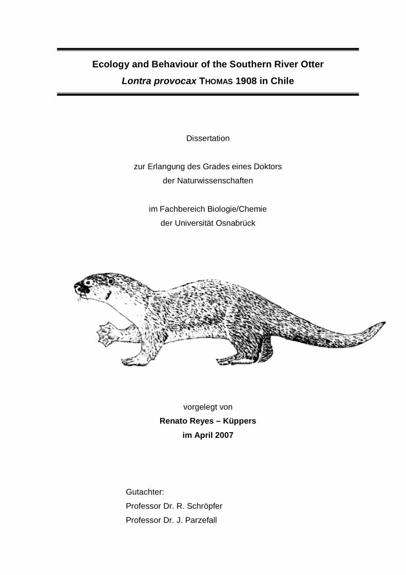
Ecology and Behaviour of the Southern River Otter
Lontra provocax THOMAS 1908 in Chile
Dissertation
zur Erlangung des Grades eines Doktors
der Naturwissenschaften
im Fachbereich Biologie/Chemie
der Universität Osnabrück
vorgelegt von
Renato Reyes – Küppers
im April 2007
Gutachter:
Professor Dr. R. Schröpfer
Professor Dr. J. Parzefall

To
MARTINA

„ Everything should be made as simple as possible,
but not simpler“.
(Albert Einstein, 1879 - 1955)

I
1 General introduction 1
1.1 Introduction 1
1.2 Aim of study 4 1.3 Study area 6
2 Methods: trapping, surgery, housing and nutrition of Lontra provocax 9
2.1 Trapping 9 2.1.1 Introduction 9 2.1.2 Method 10 2.1.3 Results 11 2.1.4 Discussion 15
2.2 Anesthetization 19 2.2.1 Introduction 19 2.2.2 Method 20 2.2.3 Results and Discussion 22
2.3 Housing and nutrition 22 2.3.1 Introduction 22 2.3.2 Method 23 2.3.3 Results 26 2.3.4 Discussion 36
3 Home range and activity patterns of the southern river otter 41
3.1 Introduction 41 3.1.1 Home Range 41 3.1.2 Habitat preferences 42 3.1.3 Activity patterns 43 3.1.4 Aims 45
3.2 Methods 46 3.2.1 Home Range 46 3.2.2 Habitat preferences 51 3.2.3 Activity patterns 52 3.2.4 Statistical analysis 54
3.3 Results 55 3.3.1 Home Range 55 3.3.2 Habitat preferences 63 3.3.3 Activity patterns 75
3.4 Discussion 84 3.4.1 Methodology 84 3.4.2 Home Range 90 3.4.3 Habitat preferences 94 3.4.4 Activity patterns 97
3.5 Prospects 101

II
4 Rearing cubs: effect on home range and activity pattern of a female southern river otter (Lontra provocax THOMAS 1908) 102
4.1 Introduction 102 4.1.1 Study site 103
4.2 Methods 104 4.2.1 Radio tracking 104 4.2.2 Activity pattern 105 4.2.3 Den sites 106 4.2.4 Data evaluation 106
4.3 Results 107 4.3.1 Home range 107 4.3.2 Activity budget 110 4.3.3 Den sites 114 4.3.4 Additional behaviour observations 115
4.4 Discussion 116 4.4.1 Home range 116 4.4.2 Activity budget 116 4.4.3 Den sites 117 4.4.4 Reproductive cycle and parental care – a model 118
5 Prey availability, diet composition and food competition 120
5.1 Introduction 120 5.1.1 Prey availability 120 5.1.2 Food competition 121 5.1.3 Diet composition 122 5.1.4 Aims 123
5.2 Methods 124 5.2.1 Sampling methods 125 5.2.2 Spraint analysis 127 5.2.3 Water analysis 128 5.2.4 Ecological parameters and statistics 131
5.3 Results 138 5.3.1 Diversity and abundance 138 5.3.2 Spraint analysis 154 5.3.3 Prey availability versus diet composition 161 5.3.4 Required quantity of staple prey 162 5.3.5 Water analysis 166
5.4 Discussion 173 5.4.1 Methodology 173 5.4.2 Prey availability 176 5.4.3 Diet composition 183 5.4.4 Seasonality 187 5.4.5 Required quantity of staple prey 189 5.4.6 Diet – mink versus otter 191
5.5 Prospects 193

III
6 Age determination of male southern river otter Lontra provocax (THOMAS 1908) 194
6.1 Introduction 194 6.2 Methods 195
6.3 Results 196 6.4 Discussion 200
7 Summary 204
8 Reference List 207
9 Acknowledgements 239
10 Appendix 241
10.1 Methods 241 10.2 Home range and activity patterns of the southern river
otter 243 10.3 Rearing cubs: effect on home range and activity pattern of
a female southern river otter (Lontra provocax Thomas 1908) 245
10.4 Prey availability, diet composition and food competition 246 10.5 Age determination of male southern river otter Lontra
provocax (Thomas 1908) 251

IV
Preface
There are 5 chapters within this thesis, with the different aspects of
methodology being discussed in Chapter 2. The thesis contains
unpublished data, however Chapters 4 and 6 have been written as a
manuscript for upcoming publication. Therefore some descriptions
regarding the study area and methodology are repeated in these
chapters.
1 General introduction 1.1 Introduction 1
1 General introduction
1.1 Introduction
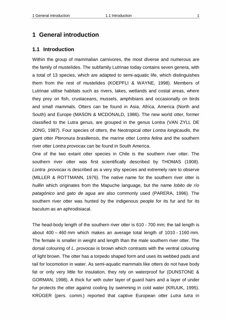
Within the group of mammalian carnivores, the most diverse and numerous are
the family of mustelides. The subfamily Lutrinae today contains seven genera, with
a total of 13 species, which are adapted to semi-aquatic life, which distinguishes
them from the rest of mustelides (KOEPFLI & WAYNE, 1998). Members of
Lutrinae utilise habitats such as rivers, lakes, wetlands and costal areas, where
they prey on fish, crustaceans, mussels, amphibians and occasionally on birds
and small mammals. Otters can be found in Asia, Africa, America (North and
South) and Europe (MASON & MCDONALD, 1986). The new world otter, former
classified to the Lutra genus, are grouped in the genus Lontra (VAN ZYLL DE
JONG, 1987). Four species of otters, the Neotropical otter Lontra longicaudis, the
giant otter Pteronura brasiliensis, the marine otter Lontra felina and the southern
river otter Lontra provocax can be found in South America.
One of the two extant otter species in Chile is the southern river otter. The
southern river otter was first scientifically described by THOMAS (1908).
Lontra provocax is described as a very shy species and extremely rare to observe
(MILLER & ROTTMANN, 1976). The native name for the southern river otter is
huillin which originates from the Mapuche language, but the name lobito de río
patagónico and gato de agua are also commonly used (PARERA, 1996). The
southern river otter was hunted by the indigenous people for its fur and for its
baculum as an aphrodisiacal.
The head-body length of the southern river otter is 610 - 700 mm; the tail length is
about 400 – 460 mm which makes an average total length of 1010 - 1160 mm.
The female is smaller in weight and length than the male southern river otter. The
dorsal colouring of L. provocax is brown which contrasts with the ventral colouring
of light brown. The otter has a torpedo shaped form and uses its webbed pads and
tail for locomotion in water. As semi-aquatic mammals like otters do not have body
fat or only very little for insulation, they rely on waterproof fur (DUNSTONE &
GORMAN, 1998). A thick fur with outer layer of guard hairs and a layer of under
fur protects the otter against cooling by swimming in cold water (KRUUK, 1995).
KRÜGER (pers. comm.) reported that captive European otter Lutra lutra in

1 General introduction 1.1 Introduction 2
Hankensbüttel/Germany were filmed with a thermograph camera and only the
pads of the animal appeared coloured, which stands for the only possibility to emit
heat. Hence it seems that becoming too cold is not the problem, but rather
preventing overheating.
The territorial behaviour was recently described by SEPULVEDA (2003) as
intrasexually territorial. Therefore adult animals are solitary and are only seen
together during mating season for copulation. Only females with their offspring
form family groups. CHANIN (1985) reports that young ones stay in family groups
in the first year until they disperse. This species is described as usually nocturnal
(CHANIN, 1985), however individual reports of diurnal behaviour by local farmer
exist.
One hundred to one hundred and fifty years ago the southern river otter had a
longitudinal distribution from the centre to the southern part of Chile. Specifically,
from the rivers Cauquenes and Cachapoal (34° S) to the Magellan Region (53° S)
and from the Andes to the Pacific (HARRIS, 1968; MEDINA-VOGEL, 1996;
MELQUIST, 1984; MILLER & ROTTMANN, 1976; OSGOOD, 1943). In the past
the southern river otter had an extensive distribution ranging from rhitron to
potamon rivers and Andean oligotrophic lakes to shallow lakes and Coastal
wetlands (CHEHÉBAR & PORRO, 1998; MEDINA & CHEHÉBAR, 2000; MEDINA-
VOGEL, 1996). From south of the XI. Región of Chile (Region of Aysén)
L. provocax was also found in marine ambience especially in the Patagonian and
Fuegian channels and straits (SIELFELD & CASTILLA, 1999). Since the European
colonisation in 1860, the southern part of Chile’s rivers and lakes have been used
as transport routes. Riparian vegetation was removed, forests cleared and wetland
turned into farm land. This interference resulted in a gradual destruction of the
habitat of the southern river otters (LARA & ARAVENA, 1997; SOTO & CAMPOS,
1997; TOLEDO & ZAPATER, 1991). Furthermore, it seems that habitat
characteristics - such as water depth, surface area, velocity of river current,
riparian vegetation, riparian and subsurface woody debris - have an impact on
prey occurrence, which in turn has a significant effect on the spatial distribution of
the otter population (CROOK & ROBERTSON, 1999; KAIL, 2005; KRUUK, 1995).
Today the distribution of the southern river otter in freshwater habitats in Chile is

1 General introduction 1.1 Introduction 3
limited to only few isolated areas between Cautín (39° S) and Futaleufú (43° 30’ S)
and it is most likely the otter species with the smallest distribution in the world
(CHEHÉBAR et al., 1986; MEDINA-VOGEL, 1996).
The southern river otter is listed internationally as CITES Appendix I, and therefore
in the EU by law 338/97 it is cited in Annex A. In the IUCN Red List of the
vertebrates the otter is assessed as ‘endangered’ (UNEP-WCMC, 2002). In the
Chilean Red List of vertebrates it is classified as ‘in danger of extinction’ (GLADE
1987) and in the National Wildlife List of Argentina the otter is listed as
‘endangered’ (CHEHÈBAR et al., 1986). The extermination of the otter started in
small river basins but expanded. Habitat destruction, stream and river diversion
and wetland drainage have contributed considerably to the decline of the southern
river otter’s distribution in the last decades and in the present (MEDINA, 1991).
Other factors like hunting, dogs, farming and water pollution are suspected of
having further endangered the southern river otters (REDFORD & EISENBERG,
1992). The lack of recolonisation is possibly the reason for the high mortality rate
or the low reproductive success.
Prior studies of the diet diversity of southern river otters in lakes and rivers were
investigated by SIELFELD (1984) MEDINA (1998; 1997), CHEHEBAR (1985;
1986) and newer ones in the Boroa wetland by GONZALEZ (2006). Briefly, the
data indicate that the southern river otter mainly preys on crustacean species and
seems to be, to an unknown degree, a specialist. Studies on the influence of
riparian vegetation, woody debris and stream morphology and the use by southern
river otters show that the animals prefer sites which are in natural conditions and
without human influence (MEDINA-VOGEL et al., 2003).
Many studies on other otter species like L. lutra or Lontra canadensis exist, while
the species which are living cryptically like the southern river otter have not been
intensively investigated and much about their ecology and behaviour is still
unknown.

1 General introduction 1.2 Aim of study 4
1.2 Aim of study
The essential aim of the present study is to gain knowledge about: a) the
behaviour and b) the factors which may effect the distribution and abundance of
the southern river otter.
Furthermore the answers to these topics will be important contributions for further
conservation programs of this endangered species and in order to maintain
biodiversity in Chile.
The objectives of the studies are:
Ø to describe individual home-ranges, core areas, travel rates, activity
patterns and movements of three southern river otters in the Upper Queule
River,
Ø to assess their preference for habitat use,
Ø to identify the effect of cubs on activity and space patterns of the parents,
Ø to examine the prey utilisation, prey availability and diversity and additional
abiotic factors which may limit prey distribution,
Ø to identify if the methodology of age determination via tooth and skull is
applicable.
Since different subject areas in this particular study will be determined, they are
briefly listed here but the specific scopes and aims are detailed elucidate in
following respective chapters.

1 General introduction 1.2 Aim of study 5
Chapter 2 deals with the aspects of trapping, surgery and housing methods for the
southern river otter. Furthermore initial investigations of basic energy needs are
examined.
In Chapter 3 the objectives of home range, activity patterns and the preference for
habitat use are presented in detail. For geographic spacing patterns the
accessibility to the animal’s home range, total range, and different levels of core
area are considered. To determine activity patterns the occurrence and duration of
movement, stationary activity and inactivity are investigated, as well as travelled
duration and distance. Also presented here are detailed measures of preferred
habitat use like hunting areas, den sites and spraint sites.
The change of spacing patterns of female with cubs was compared in Chapter 4.
Home range, travelled distance and activity patterns were also examined.
Furthermore a model is presented which illustrate the reproduction cycle of this
species.
Prey availability, diversity and abiotic factors which may limit the distribution of
prey and consequently the distribution of the southern river otter is determined in
Chapter 5. Areas of otter occurrence were investigated for potential prey like
amphibians, fish and crustaceans. For a seasonal variation of prey ingestion
spraint analysis were carried out for 12 month on the Upper Queule River. To gain
additional information of abiotic conditions water analysis on several stations was
conducted for one year. Furthermore it was determined if an interspecific
competition exist between L. provocax and the American mink Mustela vison.
Chapter 6 is about the feasibility of using tooth and skull analysis for age
determination of the southern river otter.

1 General introduction 1.3 Study area 6
1.3 Study area
Chile is a narrow land with an average width of 180 km and a length of about
4300 km between 17° 3’ S and 56° 30’ S. Except for the tropical climate all types
of climate can be found on Chile’s mainland which is strongly dependent upon the
Humboldt stream. The north of Chile is dominated by the Andes whereas central
and south Chile are formed by two parallel mountain ranges colon the costal
mountain range (Cordillera de la Costa) and the Andes, in north-south expansion.
The central valley (Valle Central), with its arable land, is situated between the two
mountain ranges.
Politically the country is divided into 13 regions. The area in which the
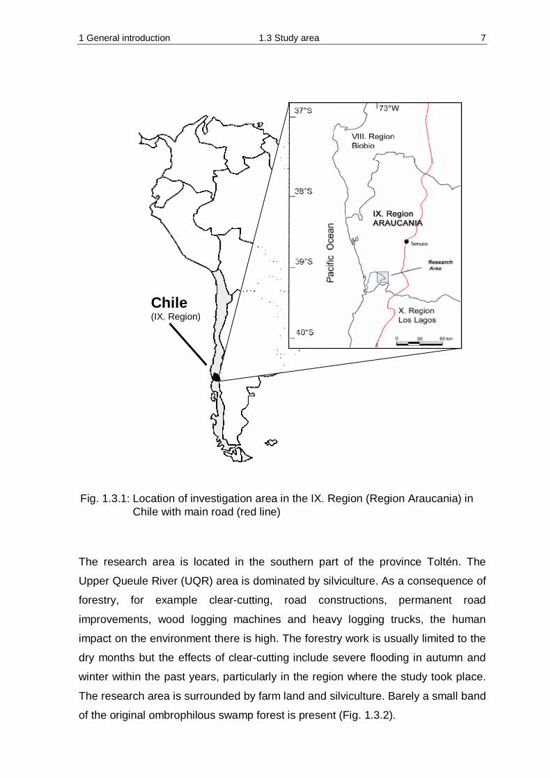
investigation was conducted lies in the IX Region, the Araucania region
(Fig. 1.3.1), which has a temperate climate. The investigated river is called Queule
and is approximately 87 km1 long, originates in the coastal mountain range at an
altitude of about 550 m (39° 12’ 45’’ S; 73° 00’ 24’’ E) and terminates at the village
Queule, where it pours into the Pacific Ocean (39° 26’ 32’’ S; 73° 12’ 59’’ E). The
Queule River is partially covered by a temperate evergreen ombrophilous swamp
forest which is composed primarily by Myrceugenia exsucca, Eleocharis
macrostachya, Scirpus californicus, Juncas procerus, Temu divaricatum and
Drimys winteri (HAUENSTEIN et al., 2002; RAMÍREZ et al., 1983). The river
currents are mainly regulated by rainfall which reaches an average of 2110 mm
per year with seasonal low level during summer time and high level during winter
time.
1 As no data of Queule River length were available, length of river was measured six times with
measuring tool in ArcView™ 3.1 and average was calculated m)106.681SE m; 87126.167x( ==
1 General introduction 1.3 Study area 7
The research area is located in the southern part of the province Toltén. The
Upper Queule River (UQR) area is dominated by silviculture. As a consequence of
forestry, for example clear-cutting, road constructions, permanent road
improvements, wood logging machines and heavy logging trucks, the human
impact on the environment there is high. The forestry work is usually limited to the
dry months but the effects of clear-cutting include severe flooding in autumn and
winter within the past years, particularly in the region where the study took place.
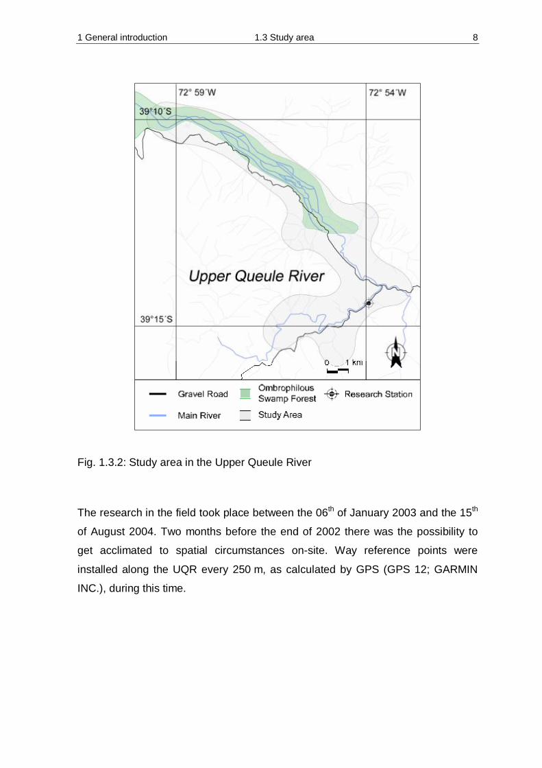
The research area is surrounded by farm land and silviculture. Barely a small band
of the original ombrophilous swamp forest is present (Fig. 1.3.2).
Fig. 1.3.1: Location of investigation area in the IX. Region (Region Araucania) in Chile with main road (red line)
Chile (IX. Region)
1 General introduction 1.3 Study area 8
Fig. 1.3.2: Study area in the Upper Queule River The research in the field took place between the 06th of January 2003 and the 15th
of August 2004. Two months before the end of 2002 there was the possibility to
get acclimated to spatial circumstances on-site. Way reference points were
installed along the UQR every 250 m, as calculated by GPS (GPS 12; GARMIN
INC.), during this time.

2 Methods 2.1 Trapping 9
2 Methods: trapping, surgery, housing and nutrition of Lontra provocax
2.1 Trapping
2.1.1 Introduction
It is very difficult to study carnivores, which usually have a cryptic and nocturnal
behaviour, are rarely observed, and seldom are leaving faeces or tracks (RUETTE
et al., 2003). Direct observations can only be made at the expense of significant
amounts of personnel, money and time. One alternative is trapping and fitting
animals with a radio transmitter, which allows researchers to conduct direct and
indirect observation of the behaviour and moving patterns of the subject. For some
animals it is possible to trap them using long-distance immobilization such as
tranquilizer darts. For other animals that are harder to find, trapping with harmless
traps is more effective but requires people to check the traps regularly. The otter,
since it lives secretly, is reported as mostly nocturnal and is very shy to any
disturbance, is one such animal for which harmless traps are most effective in
trapping (BLUNDELL et al., 1999).
In January of 2003, in the IX. Region (the Lake District) of Chile, several different
river systems were searched for signs of otters. In this process, we looked for
evidence of otter presence such as dens, footprints, faeces and smears. The
investigations were limited to the IX. Region because prior surveying and mapping
had uncovered more evidence of otters there than in other regions (pers. comm.,
MEDINA-VOGEL). We located 21 positive sites, including the upper part of the
Queule River, which was a particularly promising area because fresh faeces was
found there in several sites that were well suited to setting up our traps.
2 Methods 2.1 Trapping 10
2.1.2 Method
Trapping locations
To trap southern river otters we used “leg-hold traps” (1.5 Victor Soft Catch Trap),
which were connected to a 1.5 m iron chain link. The chain was clamped to a
12 kg block of concrete.
The areas for setting the soft-catch traps were selected according to the following
criteria:
• river depth,
• active exit; normally in connection with marking places or dens,
• possibility to fix the traps (concrete block) to the riverbed.
The traps were fixed to a level surface in the river such that they were covered by
3-5cm of water and so that the chain was not visible in the sediment. The concrete
block was also positioned under water and additionally fixed to sticks of 1 m
length, such that it could not be moved.
In other spots, such as bridges, the chain was fixed to the wooden bridge with at
least three 10cm long steel nails. Within a radius equal to the length of the chain
plus an extra of 1.5 meters, all roots and similar obstacles above and below the
water were removed with a saw to minimize the risk that the trapped animal could
become entangled and drown. After the trap was set, the manipulated riparian
bank was rinsed with water to minimize human odours. No bait was used. After the
trapping period, all traps were completely removed.
Trapping
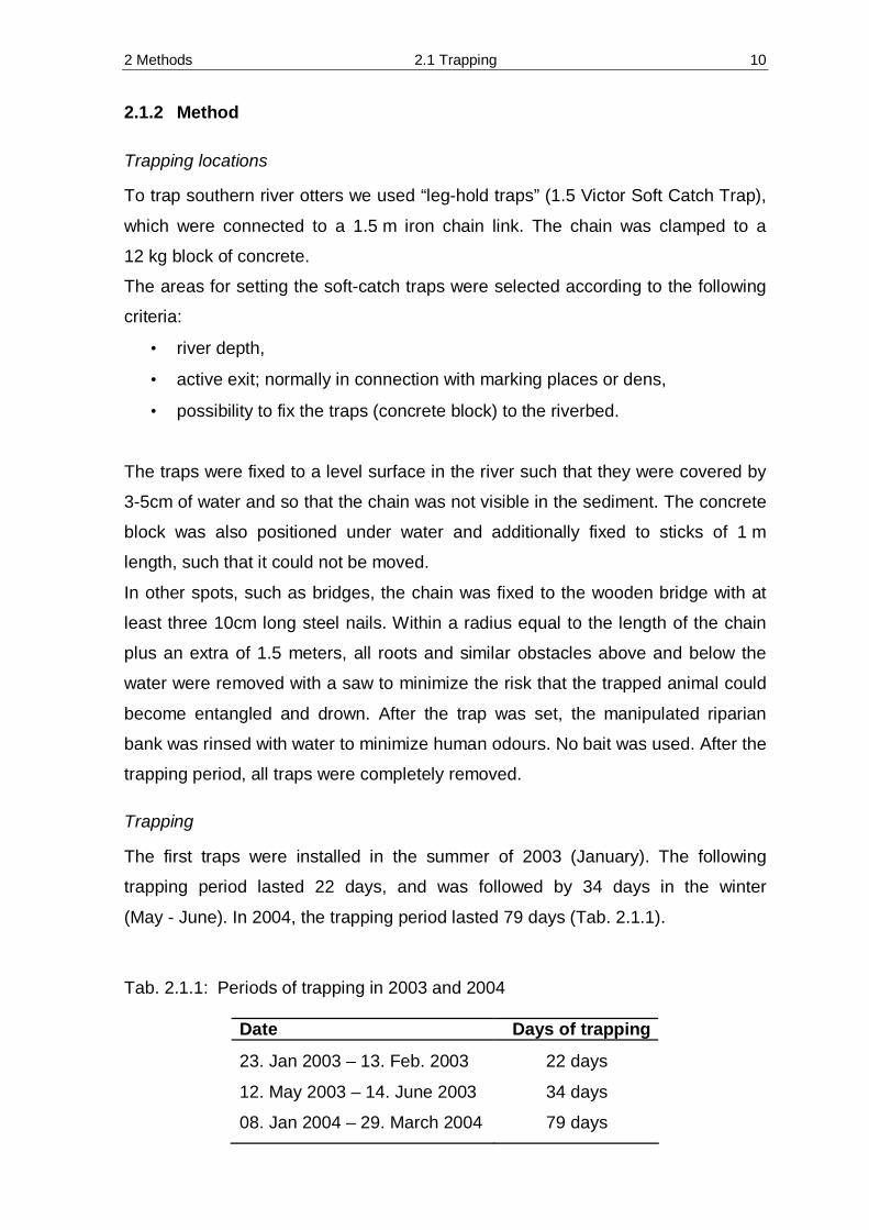
The first traps were installed in the summer of 2003 (January). The following
trapping period lasted 22 days, and was followed by 34 days in the winter
(May - June). In 2004, the trapping period lasted 79 days (Tab. 2.1.1).
Tab. 2.1.1: Periods of trapping in 2003 and 2004
Date Days of trapping
23. Jan 2003 – 13. Feb. 2003 22 days
12. May 2003 – 14. June 2003 34 days
08. Jan 2004 – 29. March 2004 79 days

2 Methods 2.1 Trapping 11
Traps were checked every 12 hours so that the animal did not become overly cool
because of prolonged submergence in the water. The checking of the traps was
performed at 08:00 in the morning and at 20:00 in the evening during the summer,
and at 06:00 in the morning and 18:00 in the evening in the winter. The reason for
the time difference between summer and winter is that we wanted to conduct the
trap inspections and potential immobilizations while there was still some light.
A trap found closed but without an animal was reactivated and the area once
again rinsed with water.
In the case that animals other than otters were caught ("bycatch"), if not already
drowned, we removed them from the trap, medicate them, and after a period of
convalescence, released them back into the wild.
2.1.3 Results
The results of the trappings are illustrated in the following table (Tab. 2.1.2). The
part of the river where the trappings were performed was divided into two sections
(upper - and lower). The upper section was mainly influenced by arable farm land
and pine plantation, in strong contrast to the lower section, which was covered
with a temperate evergreen ombrophilous swamp forest - called “Hualve”.
Because of the low trapping success in the summer of 2003 (only one adult female
was caught), an additional trapping period for the winter season was decided upon
for the first time.
In spite of heavy precipitation and the resulting strong fluctuations of water level,
we succeeded in trapping another southern river otter (an adult male). After an
additional 27 days with very little indication of otter activity, heavy precipitation,
and very low air and water temperature, the trapping season was terminated. In
the summer of 2004 (January), the trapping area was extended further down the
lower section of the river.
In 2003, over a length of 7.3km, and in 2004, over a length of 11.1 km, on average
24 active traps were set. Out of 1662.5 trapping nights, the success rate for
trapping otters was 0.002. In the upper section of the Queule River, during 2003
and 2004 a total of five southern river otters were trapped, whereas only one
animal was caught in the lower section. The density of southern river otters
represents 0.4 animals per kilometre. Among the captured animals were two adult

2 Methods 2.1 Trapping 12
females, one juvenile male and three adult males. A total of three animals died,
including one juvenile and two adult males.
Table 2.1.2: Trapping success (F = adult female; M = adult male; m = juvenile
male, * = average)
Specific location 2003 2004 Total* Upper section 1F/1M 1m/2M 1F/1m/3M Lower section 0 1F 1F Total number of otters 1F/1M 1F/1m/2M 2F/1m/2M Identified dead otters 1M 1m/1M 1m/2M Distance covered (km) 7.3 11.1 9.2 Average active traps 22 - 26 (24*) 18 - 29 (24*) 24 Number of night 55 79 67 Number of traps/night 1340 1985 1662.5 Otters per traps/night 0.002 0.002 0.002 Otters/kilometres 0.3 0.4 0.4 One otter per kilometres 3.70 2.80 3.25
2 Methods 2.1 Trapping 13
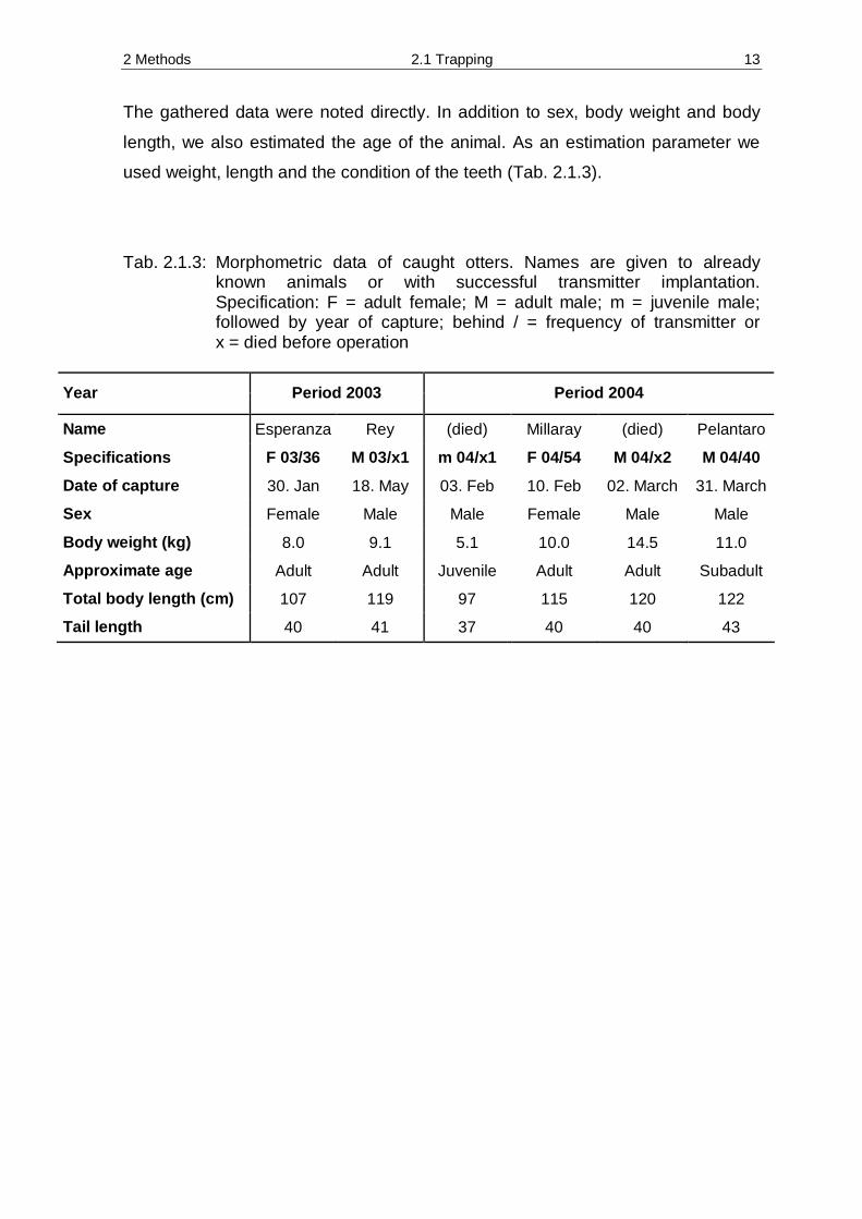
The gathered data were noted directly. In addition to sex, body weight and body
length, we also estimated the age of the animal. As an estimation parameter we
used weight, length and the condition of the teeth (Tab. 2.1.3).
Tab. 2.1.3: Morphometric data of caught otters. Names are given to already known animals or with successful transmitter implantation. Specification: F = adult female; M = adult male; m = juvenile male; followed by year of capture; behind / = frequency of transmitter or x = died before operation
Year Period 2003 Period 2004
Name Esperanza Rey (died) Millaray (died) Pelantaro
Specifications F 03/36 M 03/x1 m 04/x1 F 04/54 M 04/x2 M 04/40
Date of capture 30. Jan 18. May 03. Feb 10. Feb 02. March 31. March
Sex Female Male Male Female Male Male
Body weight (kg) 8.0 9.1 5.1 10.0 14.5 11.0
Approximate age Adult Adult Juvenile Adult Adult Subadult
Total body length (cm) 107 119 97 115 120 122
Tail length 40 41 37 40 40 43
2 Methods 2.1 Trapping 14
weight (kg)
6 8 10 12 14 16
tota
l len
gth
(cm
)
100
105
110
115
120
125
130MaleFemale
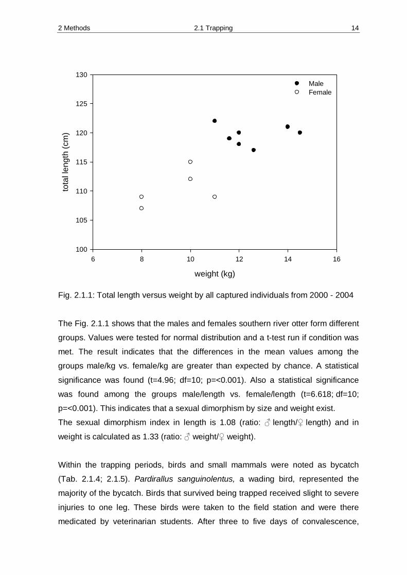
Fig. 2.1.1: Total length versus weight by all captured individuals from 2000 - 2004 The Fig. 2.1.1 shows that the males and females southern river otter form different
groups. Values were tested for normal distribution and a t-test run if condition was
met. The result indicates that the differences in the mean values among the
groups male/kg vs. female/kg are greater than expected by chance. A statistical
significance was found (t=4.96; df=10; p=<0.001). Also a statistical significance
was found among the groups male/length vs. female/length (t=6.618; df=10;
p=<0.001). This indicates that a sexual dimorphism by size and weight exist.
The sexual dimorphism index in length is 1.08 (ratio: ♂ length/♀ length) and in
weight is calculated as 1.33 (ratio: ♂ weight/♀ weight).
Within the trapping periods, birds and small mammals were noted as bycatch
(Tab. 2.1.4; 2.1.5). Pardirallus sanguinolentus, a wading bird, represented the
majority of the bycatch. Birds that survived being trapped received slight to severe
injuries to one leg. These birds were taken to the field station and were there
medicated by veterinarian students. After three to five days of convalescence,

2 Methods 2.1 Trapping 15
these animals were released. The only mammal besides otters that was caught in
the soft-catch trap was the brown rat, Rattus norvegicus, which was always found
dead in the traps.
Tab. 2.1.4: Bycatch in trapping area in both years (2003, 2004) († = died in trap because of drowning)
January 2003
February 2003
April 2003
January 2004
February 2004
March 2004
Pardirallus sanguinolentus †
Pardirallus sanguinolentus
Rattus norvegicus †
Rattus norvegicus †
Speculanas specularis
Rattus norvegicus †
Nycticorax nycticorax Rattus
norvegicus † Rattus norvegicus † Caracara plancus
Rattus norvegicus † Pardirallus
sanguinolentus † Rattus norvegicus †
Rattus norvegicus †
Pardirallus sanguinolentus
Pardirallus sanguinolentus
Pardirallus sanguinolentus †
Pardirallus sanguinolentus
Tab. 2.1.5: Scientific, English and Local names of bycatch in trapping area
Class Scientific Name English Name Local Name
Aves Pardirallus sanguinolentus Plumbeous Rail Piden
Aves Caracara plancus Southern Caracara Traro / Carancho
Aves Anas specularis Spectacled Duck Pato anteojillo
Aves Nycticorax nycticorax Black-crowned Night-Heron Huiaravo
Mammalia Rattus norvegicus Brown rat, Norway rat Guarén
2.1.4 Discussion
Trapped wild animals experience potentially high levels of stress until they are
released back into the wild. This trapping stress is described for several classes of
animals, such as reptiles (MATHIES et al., 2001), fishes (CLEMENTS et al.,
2002), birds (ROMERO & ROMERO, 2002) and mammals (ELVIDGE et al., 1976;
GERICKE & HOFMEYR, 1976; HATTINGH, 1992; LARSON & GAUTHIER, 1989;
2 Methods 2.1 Trapping 16
PLACE & KENAGY, 2000; SWART, 1992). Usually the animal attempts to flee
until it is out of danger, and therefore expends its strength by trying to get out of
the trap and does not give up easily. Other factors like unknown noises, smells,
unfamiliar surroundings, and the presence of humans, can cause additional stress
for the animals. One of the main causes of capture myopathy and mortality during
trapping is excessive stress (EBEDES et al., 2002). Therefore, when handling wild
animals, it is important to minimize the level of stress that they experience.
Capturing semi-aquatic mammals like the southern river otter turned out to be a
considerable challenge. The following factors were problematic in trapping
L. provocax.
• Trap:
The trap contained a plate of only five centimetres. The otter had to put one
of its extremities exactly on the plate in order to activate the catch
mechanism.
• Exit:
Southern river otters consistently mark their territory at the same spots on
land, but the point at which they exit the water onto the shore varies by
about one to two meters.
• Modification of exit:
To some extent the exit was very strongly modified visually, because all
roots were taken out of the water.
• Water level:
Due to strong precipitation the traps had to be adjusted to the new water
level or had to be deactivated.
• Disturbance:
Some of the traps were not visible form the bank line. One person had to go
into the water to check the trap.
• Theft:
Some of the traps were visible to other humans (like anglers and hunters),
and in three cases were stolen.

2 Methods 2.1 Trapping 17
Further disadvantages may arise by modification of the traps or exits because of
remaining odours, which could frighten off the animal and thereby decrease the
trapping success.
Some of the traps have been closed and were pulled away from their original spot
where we found hairs of otter between the rubber layers. This trapping spots were
avoided for some days, but several days later otter signs were detected again,
however otters were never captured in this traps. It seemed that the otter
remembered and stayed away from this trap. MASON & MCDONALD (1986)
mentioned the awareness of presence of traps for L. lutra in Britain.
There are different types of traps that are usually used to trap otters for research.
In Scotland, hunters have often used special otter houses to hunt these animals.
Inspired by this KRUUK (1995) built a wooden-tunnel box which was set in the
Shetland area where otters had been seen. Before being armed, the box was left
in place for years before being activated so that the otter became accustomed to
its presence. However, it would not be possible to catch the southern river otter
with a wooden-tunnel box, because of the precipitation and out of it resulting
fluctuation of the river level. Within three to four hours the river level can arise
rapidly and flood larger areas. On the other hand, thievery is a serious problem
and it could be possible that persons will illegally hunt the southern river otter with
this kind of traps. In addition, the right setting for the wooden-tunnel box would be
difficult due to the animals’ behaviour. It seems that the animal is very strong
bound to the water and do not walk larger distances (for example: marking sites
are very close to the river), since the otter never has been seen further away than
three meters from the river (southern river otters only left the water for marking).
For this study another type of trap which was originally used by fur trappers was
applied. The teeth were flattened and covered with rubber to not harm the animal.
These traps have already been used to successfully trap otters (BLUNDELL et al.,
1999; FERNÁNDEZ-MORAN et al., 2002; MELQUIST & HORNOCKER, 1983;
MITCHELL-JONES et al., 1984), as well as other mammals like beavers
(WHEATLEY, 1989), cats (MEEK et al., 1995); (SHORT & TURNER, 2005), foxes
and wild dogs (FLEMING et al., 1998).
RUETTE (2003) and SHORT (2001) demonstrated that trapping experience had
significant affect of capture rates on small carnivores and mammals. Therefore,
2 Methods 2.1 Trapping 18
people from previous trapping seasons (2000 – 2002) supported us in setting traps
to avoid a negative effect.
The trapping period was usually chosen in summer because of weather conditions
and former experiences. However, in summer 2003 less otter activity as in the last
years were recorded. A possible explanation for the low activity could be the very
low water level during the summer in the upper part of the Queule River.
Therefore, for the first time trapping was conducted also in the winter period.
However, otter activity was not very high. More otter activity occurred in summer
2004 where four animals were caught.
In comparison to trapping of the southern river otter in previous years
(2000 - 2002) were the trapping success three times higher, 0.006 otters per
trapnight (unpublished data), than in our study (0.002 otters per trapnight).
One of the causes for less otter activity and trapping success could be the clear
cutting of the surrounding pine plantation. Roads were rebuilt for the heavy logging
machines and soil, rocks and trees have been pushed into the river. Heavy logging
trucks were working for several weeks in 24-hour shifts and the roads are mostly
situated very close to the river.
All animals appeared healthy, except for M 03/x1, which was captured in the
winter of 2003. This adult male was a recaptured animal which had lost a
significant amount of weight since its previous capture (2000 = 12.6 kg;
2001 = 10.0 kg; unpublished data by MEDINA-VOGEL).
Sexual dimorphism is also reported in L. provocax (LARIVIÈRE, 1999b) as well as
in other Lontra species, such as the neotropical river otter Lontra longicaudis
(LARIVIÈRE, 1999a) and the northern river otter Lontra canadensis (LARIVIÈRE &
WALTON, 1998). An exception is the marine otter Lontra felina, which does not
show sexual dimorphism (LARIVIÈRE, 1998).
In the review by LARIVIÈRE (1999b), sexual dimorphism for L. provocax is
reported by OSGOOD (1943), whereby the female otters are approximately 90 %
the size of males. These findings are similar to our data where females were in
average 92 % of the size of males.
My results indicate that the sexual dimorphism in length is very small
(♂ = 119.57 cm, ♀ = 110.40 cm; sexual dimorphism index of 1.08). However, all
female animals were under the length of 115 cm (107 – 115 cm) and all adult male
otters were ≥ 117 cm (117 – 122 cm) long.
2 Methods 2.2 Anesthetization 19
A sexual dimorphism was also found in the weight (♂ = 12.53 kg, ♀ = 9.4 kg;
sexual dimorphism index of 1.33), where the female otters were 75 % the weight
of males. The juvenile m 04/x1 and adult M 03/x1 (a recaptured animal who's
weight had decreased since 2000) were omitted from the calculations.
I conclude that the statistical significant findings on sexual dimorphism, average
weight and average length are more probable than those reported in former
literature, because in this study the sample size was larger, and their findings on
average weight and length were based on only four samples.
The leg-hold traps like this one used in our study have to be installed in shallow
water and therefore it is especially problematic for warding birds, since three out of
ten birds drowned and one of the species which were caught, Anas specularis, is
listed in the IUCN Red list as low risk/near threatened (IUCN, 2004). It is possible
that the birds were attracted by the shininess of the activation plates, since they
were usually trapped in very new traps where the plate was still very shiny and not
oxidised as it was in the older ones. When setting the traps we tried to spread
sand from the riverbed over the plate to camouflage it, but the current of the river
often washed this sand away. It seems that bycatch such as warding birds may be
unavoidable as it also is reported by trapping Eurasian otters in Spain by
SAAVEDRA (2002).
2.2 Anesthetization
2.2.1 Introduction
Medical immobilization was conducted for rescuing endangered animals, such as
antelope, for the first time at the end of the 1950s in Africa. This technique, which
originates from the Indians of the tropical forest, is nowadays widely used for
handling wild animals. These days the medication for immobilisation is more
sophisticated and the rate of mortality is reduced. Usually a combination of
neuroleptica and analgetica is given to the animal, but it has to be considered that
even animals within the same family or genus do not react equally to the drugs
(GÖLTENBOTH, 1995; LÖSCHER, 2002).
For the southern river otter, first a Ketamin-Xylazin combination was used, but in
2004 the medical treatment for sedation and anesthetization was different. In 2004
2 Methods 2.2 Anesthetization 20
it was possible to obtain different drugs which were already successfully tested on
other otter species (LEWIS, 1991; SPELMAN et al., 1994; SPELMAN, 1999). A
detailed description of the sedation and anesthetization on the L. provocax in 2004
is described by SOTO-AZAT et al. (in press).
2.2.2 Method
Sedation
Traps were checked by two people, because for the sedation of the otter at least
two people are required. The animal was immobilized by one person with a
telescope bar. This procedure consisted of a rubber isolated metal loop being put
under its arm and around the neck and then tightened. The second person
conducted the sedation with a mixture of Ketamin (Imalgene®) and Xylazin
(Rompun®) which was injected in the muscle of its hind leg (longissimus dorsi).
Ketamin effects a rapid immobilisation, loss of consciousness and extensive
analgesia. Xylazin, in addition to having strong tranquilizing and strong central
relaxing effects, is the only neuroleptic that causes an animal specific analgesia.
The advantages of a Ketamin-Xylazin combination include better muscle
relaxation, less strain on the circulatory system than with Ketamin alone, and more
immediate, painless, and reliable effectiveness than with just Xylazin (HATLAPA &
WIESNER, 1982). In contrast to other sedation medications, there is no antidote
for Xylazin.
The dose rate was based on the condition and calculated weight of the trapped
animal; 9.61 mg/kg Ketamin, as well as 0.4 mg/kg Xylazin.
Once an animal was sedated and no longer aggressive, the traps were opened
and the animal taken to the river bank. The eyes of the sedated animal were
covered with a cloth, the respiratory track was checked to prevent obstruction, and
the otter was examined for injuries caused by the trap. Aseptic inflammation of the
foot pad caused by the trap, was treated with the intramuscular application of
0.1 mg/kg Dexamethason (Dispert dex®). Additionally, we applied to their eyes an
eye drop combination supplement (Mixgen®), the main components of which,
Bethamethason and Gentamicin, have an anti-infectious and anti-inflammatory
effect. Furthermore it protects the cornea against desiccation.

2 Methods 2.2 Anesthetization 21
The sedated animal was then transported in a coarsely meshed hard plastic net in
a heated vehicle to the enclosure at the field station.
A broad spectrum anthelmintic (Drontal plus®) containing a combination of
Febantal (for cestodes), Praziquantel, and Pyranteembonat (for nematodes) was
given to the otter.
Animals that showed infections caused by trapping were given an additional broad
spectrum antibiotic (Baytril®) via their food.
The injuries were treated with a 10 % iodine solution (Betadine®). This iodine
solution was sprayed onto the wound through the fence from outside the enclosure
while the animal was fed. Furthermore, vitamin supplements (Longvid®) were
given daily in tablets.
Anesthetization / Surgery
On earlier studies it was tried to use collars or harness to track river otter but there
is the danger that the animals become stuck (MASON & MCDONALD, 1986).
Therefore, the most appropriate method is to use implanted radio transmitter, as
well as no influence or negative effects on the reproduction were noted in studies
on L. lutra (REID et al., 1986).
Animals were starved for eight hours prior surgery. For the placement of the
intraperitoneal radio transmitter, anaesthesia was carried out as described above
for sedation. Therefore, the animal was fixed with a nyliner in his PVC tube and an
intramuscular injection was given. For the surgery the animal was fixed to the table
by its limbs. After shaving a small part of the abdominal region, a short incision of
four to five centimetres was made and the southern river otter was examined for
an old radio transmitter. In the case the animal was a recapture the old radio
transmitter was removed and replaced with a new one. The new radio transmitter
(Sirtrack Ltd., Havelock North 4201, New Zealand) was activated by a magnet,
checked with the receiver for function and after sterilization was placed in the
abdominal cavity. For the placement of the transmitter it has to be ensure that it
does not interfere with body functions (SMITH, 1980). Within 45 minutes the
operation was completed. The animal was put convalescence into a smaller cage
that was connected with its former PVC tube.
2 Methods 2.3 Housing and nutrition 22
2.2.3 Results and Discussion
All animals showed very aggressive behaviour when trying to sedate them. The
trapped and sedated animals were taken immediately to their cages and provided
with a bowl of water. The otter F 03/36 left the tube immediately and tried to move
around the cage, whereas the male M 03/x1 remained in its tube. Both animals
showed hallucinations and hissed. Ketamin is known to produce hallucinations
after recovery (HATLAPA & WIESNER, 1982). After 1.5 hour the animals
displayed normal behaviour.
All trapped animals were more or less injured by the trapping procedure. The
healing of the wound on the trapped paw took up to ten days. All otters used their
injured paw while walking in the cage. Therefore the impact of the injury was
recognized as not severe.
During the operation of the adult female F 03/36 while the transponder was
interperitoreal set, the animal suffered two times of apnoea, but in the end fully
recovered. Most likely this was due to recirculation of anaesthetic drug. The animal
was then returned to its smaller cage where it regained consciousness and
displayed behaviour typical for individuals recovering from the sedation from the
trap, namely hallucinations and hissing. After 1.5 hours the otter seemed to have
recovered and was again drinking water.
2.3 Housing and nutrition
2.3.1 Introduction
Captured animals that are released within an enclosure are confronted with a new
situation in which their space and range of behaviour patterns are limited and they
respond with stress on external stimulus. Most animals adapt very quickly to the
new environment when the environment is quiet and escape is impossible
(EBEDES & VAN ROOYEN, 2002).
Animals that are not kept in species-appropriate enclosures may display abnormal
behaviour, such as stereotypic pacing and head movements, aggression and fur
plucking, all of which can be interpreted as an indicator of reduced welfare

2 Methods 2.3 Housing and nutrition 23
(GILLOUX et al., 1992). Nowadays zoos in particular are emphasizing behaviour
enrichment of their animals, introducing devices like feeding boxes or puzzle
feeders in order to minimize abnormal behaviour. In our study, animals were held
captive for less than 25 days and therefore no environmental enrichment was
necessary or performed. However, to limit the stress factor for the southern river
otter, human contact with the animal was minimized by limiting visitors to the
research camp, and performing only the necessary work, like feeding and cleaning
the enclosure, all in the intention of reducing the stress of the animals (HOSEY,
2006).
2.3.2 Method
Housing
Animals were sheltered in wire mesh enclosures with a volume of
250 x 250 x 170 cm and with a lattice door of 50 x 50 cm. The enclosures included
a pool of 200 x 200 x 50 cm, narrow resting places on the side, a six-litre
freshwater bowl and a plastic tube with wooden guillotine doors in the front and on
the back, for possible withdrawal. The tubes were shaded with an extra cover to
prevent overheating.
The main enclosures were fenced on the side and top additionally, so that no
external person had entrance to the main enclosures. A jute cloth was placed in
the cage, which was used by the animals for padding in their plastic tube. During
the trapping season, animals were kept in enclosures long enough to avoid
trapping the same animal twice.
Before entering the main cage, rubber boots were disinfected in a basin outside.
The enclosure was cleaned daily of faeces and leftover food, and the water pool
and jute cloth were changed as well.
After the operation, the animals were kept in a 40 x 48 x 90 cm cage that was
connected to the plastic tube in which they were initially kept. The cage and the
tube were set on concrete blocks so that the faeces could drop through the cage
and be less likely to infect any wounds.
Furthermore, the small cage made treating their wounds easier since their
movement was restricted and the otter forced to hold still.

2 Methods 2.3 Housing and nutrition 24
Treated animals were checked regularly and their wounds treated with iodine
during feeding. After eight days of operation animals were released at the site at
which they were originally caught.
Nutrition
The diet of the southern river otter is comprised primarily of crustaceans
(EBENSPERGER & BOTTO-MAHAN, 1997; MEDINA, 1998). As crustaceans
were unavailable, fresh sea silverside fish Odontesthes regia were used instead
while the southern river otters were kept in their enclosures. These fish, which
occurs in the pacific, brackwater and fresh water, were bought fresh and gutted at
the market in Valdivia. The fish was kept cool in ice while being transported to the
field station and once there were frozen with a gas-powered freezer. Before
feeding, the fish was thawed for 12 hours in the refrigerator, and then prepared
with medication. The otters were given this meal four times a day. To calculate the
fish intake, the weight of the offered fish and its remains after feeding were both
recorded.
To calculate the energy intake, gutted Odontesthes regia was calometrically
measured at the Institute of Animal Production at the University Austral of Chile,
Valdivia (Instituto Producción Animal, Universidad Austral de Chile). The caloric
content for Odontesthes regia was 125 kcal/100g.
To estimate the energy intake for a given otter, the consumed fish was converted
into kcal using this value (125 kcal/100g). Data on energy intake do not exist for
L. provocax; hence data from L. lutra were used for comparison.
Since the food consumption is related to their condition, the condition index K is
calculated for all animals at the time of trapping.
The condition index was based on the formula by LE CREN (1951; mentioned in
KRUUK 1995) who calculated the relationship between average weight and
average body length of fish which he expressed as (W = weight in kg, L= total
length) baLW = ,
and therefore: baLWK /= .

2 Methods 2.3 Housing and nutrition 25
If the condition index is K = 1, then the otter is deemed healthy and normal. On the
other hand, an overweight individual could have a K value of 1.4 and an
underweight one could have a condition index as low as K = 0.5 (KRUUK, 1995).
KRUUK (1995) calculated the constants a and b from 25 L. lutra road-kill samples.
The constants for female otters are a = 5.02, b = 2.33 and for males a = 5.87,
b = 2.39. The calculated condition index for females is:
33.202.5/ LWK = ,
and for males
39.287.5/ LWK = .
The condition index with the calculated constants from KRUUK (1995) was also
used for calculations on the southern river otter. However, most animals had a K
value > 1, including even the females and the male m 03/x1 which had lost 3.5 kg
between 2000 and 2003. Therefore, the constants a and b were newly calculated
for the southern river otters which were captured from 2000 to 2004 (n = 12). Data
for animals which lost weight during this time were not taken into calculation.
Based on observations of four otters sheltered in a large enclosure including a
swimming pool, KRUUK (1995) concluded a daily ingestion of 11.9 to 12.8 percent
of body mass. However, KRUUK (1995) suggests using a more conservative
estimate of 15 percent of body mass per day, which will be used to allow
comparison of the existing data on the Eurasian otter to that which were found on
the southern river otter. This percentage will be converted to the caloric content for
the sea silverside fish measured at the University Austral of Chile. For further
comparison the resting metabolic rate (RMR) will be used as described in KRUUK
(1995) as 3.2 W kg-1.

2 Methods 2.3 Housing and nutrition 26
2.3.3 Results
ln length (m)
0,06 0,08 0,10 0,12 0,14 0,16 0,18 0,20
ln w
eigh
t (kg
)
1,8
2,0
2,2
2,4
2,6
2,8
F
F
F
F
F
F
M
M
M
M
M
M
ln W = 1.844 + (3.955 ln L)
Fig. 2.3.1: Logarithms length-weight relationship of captured southern river otter
(n = 12). F = adult females; M = adult males Length and weight of all captured otters were transformed to natural logarithm and
a linear regression was calculated (see Appendix 10.1) which resulted in the
equation: 96.332.6/ LWK = .
I calculated for females a = 6.780, b = 3.130, and for males a = 6.639, b = 3.719.
The condition index can now be calculated for females as
13.378.6/ LWK = ,
and for males as 72.364.6/ LWK = .

2 Methods
2.3 Housing and nutrition
27
Tab. 2.3.1: Days in captivity (sorted by date of capture). M = male, F = female, capital letter = adult, small letter = juvenile,
† = died, rel. = released
ID
Animals
Date of capture
Days in enclosure
Date of operation
Days in small cage
Date of release or death
Days in captivity
Condition index K
F 03/36 Esperanza 30. Jan 2003 15 14. Feb 2003 8 rel. 21. Feb 2003 23 0.95
M 03/x1 Rey 18. May 2003 7 -- -- † 24. May 2003 7 0.71
m 04/x1 -- 03. Feb 2004 12 -- -- † 14. Feb 2004 12 (0.68)
F 04/54 Millaray 10. Feb 2004 14 24. Feb 2004 8 rel. 02. Mar 2004 22 0.95
M 04/x2 -- 02. Mar 2004 -- -- -- † 02. Mar 2004 1 1.10
M 04/40 Pelantaro 29. Mar 2004 2 31. Mar 2004 8 rel. 07. Apr 2004 10 (0.79)
The days in captivity, especially in the big enclosure varied among the animals due to the trapping season and success. After
the operation, the animals were kept as short as possible but minimum eight days. When no problems for wound heeling
occurred they where liberated after the eight day.

2 Methods Additional information 28
0 2 4 6 8 10 12 14 16 18 20 22 24 260
250
500
750
1000
1250
1500
1750
2000
2250
2500F 03/36
0 2 4 6 8 10 12 14 16 18 20 22 24 260
250
500
750
1000
1250
1500
1750
2000
2250
2500M 03/x1
0 2 4 6 8 10 12 14 16 18 20 22 24 260
250
500
750
1000
1250
1500
1750
2000
2250
2500F 04/54
0 2 4 6 8 10 12 14 16 18 20 22 24 260
250
500
750
1000
1250
1500
1750
2000
2250
2500M 04/40
0 2 4 6 8 10 12 14 16 18 20 22 24 260
250
500
750
1000
1250
1500
1750
2000
2250
2500m 04/x1
Fig. 2.3.2: Curve of daily kcal intake. F = adult female; M = adult male;
m = juvenile male; followed by year of capture; behind / frequency of transmitter or x = died before operation
The chronological sequence of daily ingestion is shown in Fig. 2.3.2. Only the
adult female F 03/36 ate more than 1500kcal from the beginning. The other otters
took several days to become accustomed to eating the fish. The low kcal intake for
Inge
stio
n in
cap
tivity
(kca
l)
Days of fish consumption

2 Methods Additional information 29
the otters F 03/36 and F 04/54 in the 15th day was due to the operation. The
operation on M 04/40 was conducted on its third day in captivity, rather than on the
15th, as was the case with the others.
Animals
F 03/36 M 03/x1 F 04/54 M 04/40 m 04/x1
Kca
l of f
ish
inta
ke
0
100
200
300
400
500
600
700
Fig. 2.3.3: Average kcal intake per feeding in captivity. F = adult female; M =
adult male; m = juvenile male; followed by year of capture; behind / frequency of transmitter or x = died before operation
The average amount of fish eaten per feeding session for all captured animals is
shown in Fig. 2.3.3. No significant differences were found with an analysis of
variance of the average fish eaten per feeding session (One-way ANOVA: F=2.02;
df=4; p=0.102). The average kcal intake for all otters per feeding was
(390.69 ± 98.32) kcal. The median for F 03/36: 359.38 kcal (311.25/410.47);
M 03/x1: 467.81 kcal (457.18/487.50); F 04/54: 445.31 kcal (355.16/497.66);
2 Methods Additional information 30
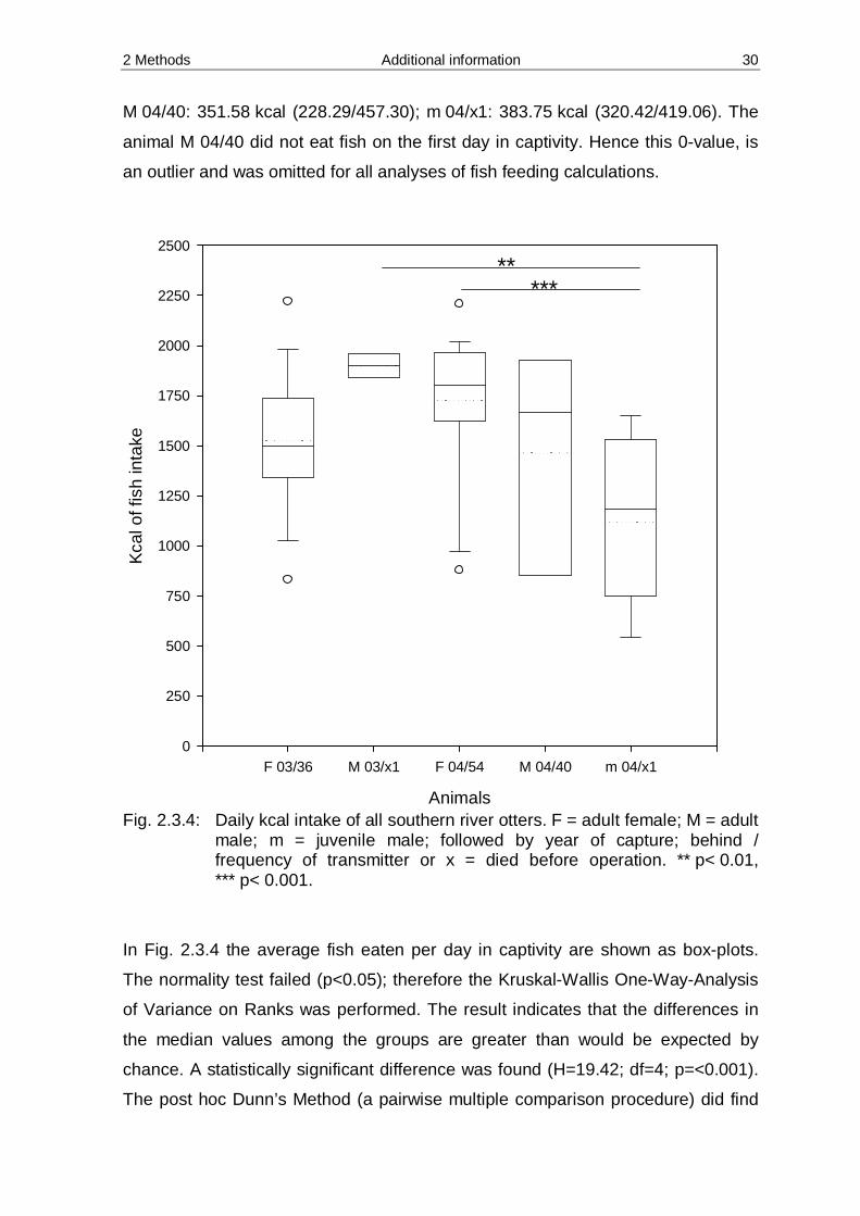
M 04/40: 351.58 kcal (228.29/457.30); m 04/x1: 383.75 kcal (320.42/419.06). The
animal M 04/40 did not eat fish on the first day in captivity. Hence this 0-value, is
an outlier and was omitted for all analyses of fish feeding calculations.
Animals
F 03/36 M 03/x1 F 04/54 M 04/40 m 04/x1
Kcal
of f
ish
inta
ke
0
250
500
750
1000
1250
1500
1750
2000
2250
2500**
***
Fig. 2.3.4: Daily kcal intake of all southern river otters. F = adult female; M = adult
male; m = juvenile male; followed by year of capture; behind / frequency of transmitter or x = died before operation. ** p< 0.01, *** p< 0.001.
In Fig. 2.3.4 the average fish eaten per day in captivity are shown as box-plots.
The normality test failed (p<0.05); therefore the Kruskal-Wallis One-Way-Analysis
of Variance on Ranks was performed. The result indicates that the differences in
the median values among the groups are greater than would be expected by
chance. A statistically significant difference was found (H=19.42; df=4; p=<0.001).
The post hoc Dunn’s Method (a pairwise multiple comparison procedure) did find
2 Methods Additional information 31
significant differences between M 03/x1 vs. m 04/x1 and F 04/54 vs. M 04/x1. The
median for F 03/36 is 1500 kcal (1361.56/1691.88), for M 03/x1: 1896.25 kcal
(1841.88/1953.75), for F 04/54: 1802.50 kcal (1638.44/1961.25), for M 04/40:
1664.06 kcal (1024.13/1903.00) and for m 04/x1: 1181.25 kcal (774.38/1489.06).
Animals
F M
Kcal
of f
ish
inta
ke
0
250
500
750
1000
1250
1500
1750
2000
2250
2500
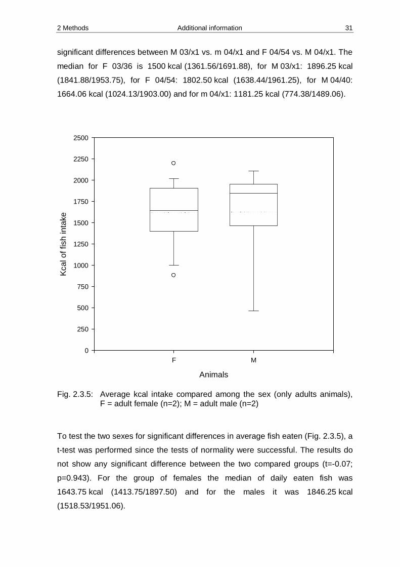
Fig. 2.3.5: Average kcal intake compared among the sex (only adults animals),
F = adult female (n=2); M = adult male (n=2)
To test the two sexes for significant differences in average fish eaten (Fig. 2.3.5), a
t-test was performed since the tests of normality were successful. The results do
not show any significant difference between the two compared groups (t=-0.07;
p=0.943). For the group of females the median of daily eaten fish was
1643.75 kcal (1413.75/1897.50) and for the males it was 1846.25 kcal
(1518.53/1951.06).
2 Methods Additional information 32
Animals
Adult Juvenile
Kca
l of f
ish
inta
ke
0
250
500
750
1000
1250
1500
1750
2000
2250
2500
***
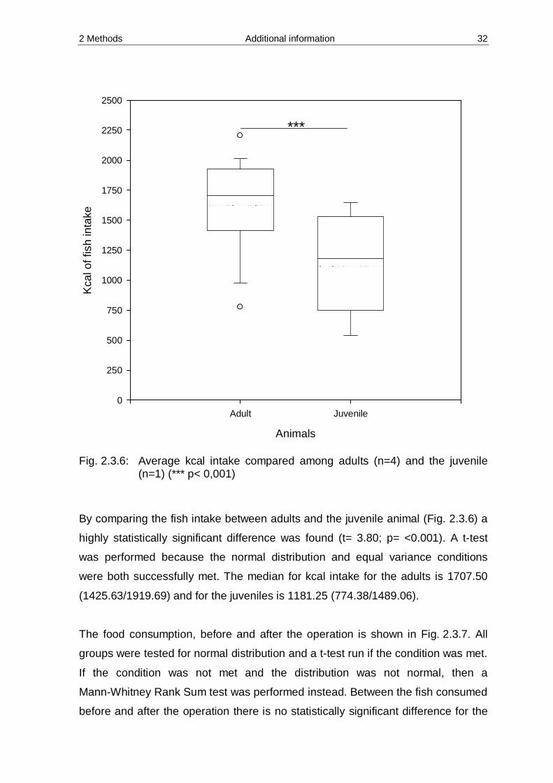
Fig. 2.3.6: Average kcal intake compared among adults (n=4) and the juvenile
(n=1) (*** p< 0,001)
By comparing the fish intake between adults and the juvenile animal (Fig. 2.3.6) a
highly statistically significant difference was found (t= 3.80; p= <0.001). A t-test
was performed because the normal distribution and equal variance conditions
were both successfully met. The median for kcal intake for the adults is 1707.50
(1425.63/1919.69) and for the juveniles is 1181.25 (774.38/1489.06).
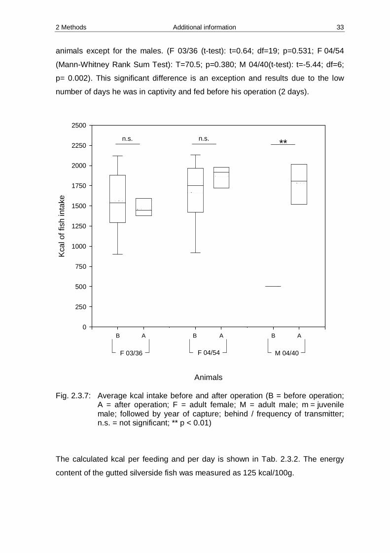
The food consumption, before and after the operation is shown in Fig. 2.3.7. All
groups were tested for normal distribution and a t-test run if the condition was met.
If the condition was not met and the distribution was not normal, then a
Mann-Whitney Rank Sum test was performed instead. Between the fish consumed
before and after the operation there is no statistically significant difference for the
2 Methods Additional information 33
animals except for the males. (F 03/36 (t-test): t=0.64; df=19; p=0.531; F 04/54
(Mann-Whitney Rank Sum Test): T=70.5; p=0.380; M 04/40(t-test): t=-5.44; df=6;
p= 0.002). This significant difference is an exception and results due to the low
number of days he was in captivity and fed before his operation (2 days).
Animals
B A B A B A
Kca
l of f
ish
inta
ke
0
250
500
750
1000
1250
1500
1750
2000
2250
2500
M 04/40F 03/36 F 04/54
n.s. n.s. **
Fig. 2.3.7: Average kcal intake before and after operation (B = before operation;
A = after operation; F = adult female; M = adult male; m = juvenile male; followed by year of capture; behind / frequency of transmitter; n.s. = not significant; ** p < 0.01)
The calculated kcal per feeding and per day is shown in Tab. 2.3.2. The energy
content of the gutted silverside fish was measured as 125 kcal/100g.
2 Methods Additional information 34
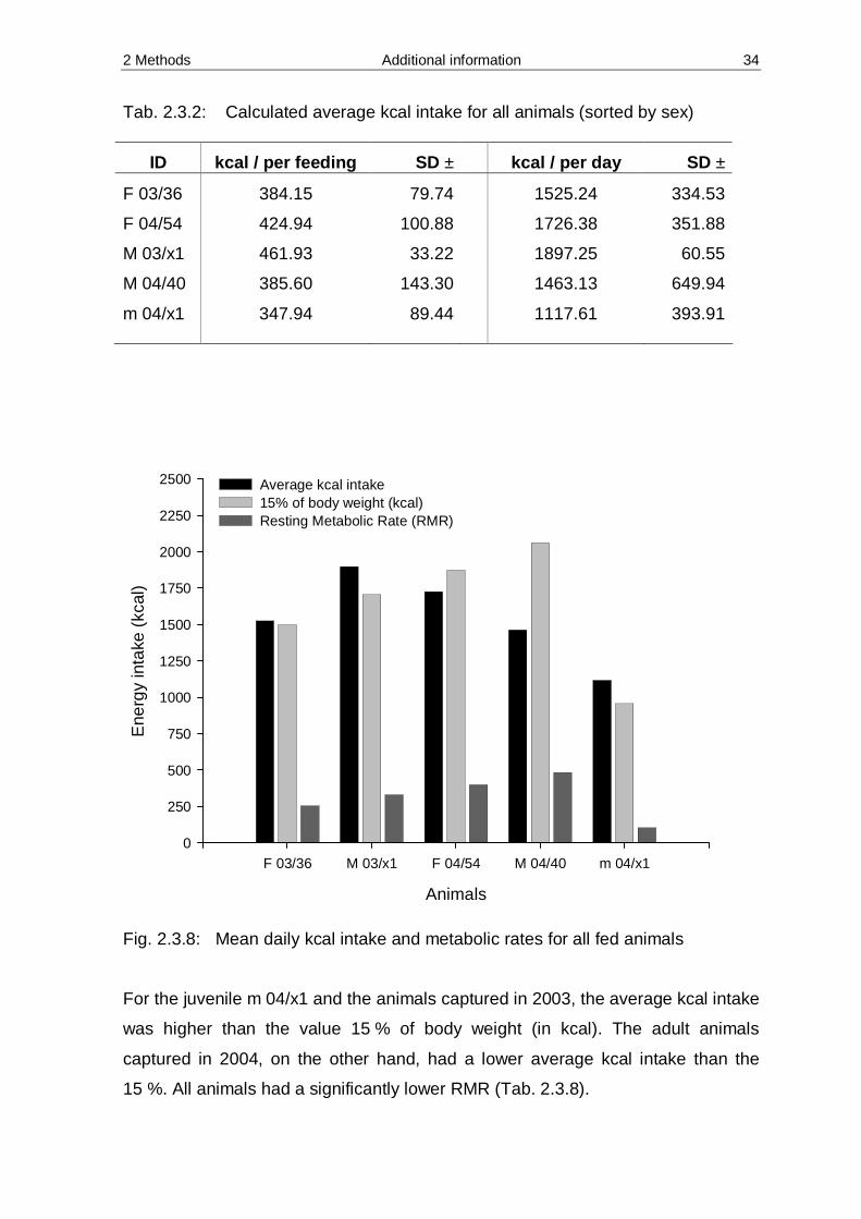
Tab. 2.3.2: Calculated average kcal intake for all animals (sorted by sex)
ID kcal / per feeding SD ± kcal / per day SD ±
F 03/36 384.15 79.74 1525.24 334.53
F 04/54 424.94 100.88 1726.38 351.88
M 03/x1 461.93 33.22 1897.25 60.55
M 04/40 385.60 143.30 1463.13 649.94
m 04/x1 347.94 89.44 1117.61 393.91
Animals
F 03/36 M 03/x1 F 04/54 M 04/40 m 04/x1
Ene
rgy
inta
ke (k
cal)
0
250
500
750
1000
1250
1500
1750
2000
2250
2500 Average kcal intake15% of body weight (kcal)Resting Metabolic Rate (RMR)
Fig. 2.3.8: Mean daily kcal intake and metabolic rates for all fed animals For the juvenile m 04/x1 and the animals captured in 2003, the average kcal intake
was higher than the value 15 % of body weight (in kcal). The adult animals
captured in 2004, on the other hand, had a lower average kcal intake than the
15 %. All animals had a significantly lower RMR (Tab. 2.3.8).

2 Methods Additional information 35
Condition index K
0,60 0,70 0,80 0,90 1,00 1,10
Ener
gy in
take
(kca
l)
0
1250
1500
1750
2000
2250FemaleMale
Fig. 2.3.9: Relation between kcal intake and condition index K for four adult
animals In contrast, the female southern river otters, which had approximately the same
condition index regardless of the level of energy intake, the males had different
condition indices for different energy intake levels. Specifically, a male otter with a
low condition index had a higher energy intake than a male otter with a high
condition index (Fig. 2.3.9).

2 Methods Additional information 36
2.3.4 Discussion
Condition Index
The condition index K was calculated for the southern river otters using only adult
animals and no recaptures. Due to the limited morphometric and demographic
data on these animals, only 12 individuals could be used in the calculations. In
contrast to KRUUK (1995), no southern river otter from road mortality could be
used for K-index calculation because values for dead otters found on the road
have never been reported. It seems that this otter species is very restricted to the
water. Therefore only adult, apparently healthy animals were used.
Both females (F 03/36; F 04/54) have the same condition index ( 95.0=K ) and
were close to the category of healthy normal otter, in contrast to the adult male
otters, of which only the male southern river otter M 04/x2 was healthy ( 1≥K ).
The condition index of the recaptured animal M 03/x1 was low and in comparison
to previous years, had decreased (2000, 13.1=K ; 2001: 78.0=K ; 2003:
71.0=K ). I took into consideration that this animal already reached his age limit,
which could also have been a reason for his death while in captivity. The K-Index
for the juvenile m 04/x1 ( 68.0=K ) and for the subadult southern river otter
M 04/40 ( 79.0=K ) are very low, probably because of age, since they were not
full-grown. The result is that the calculations for the K-index of southern river otters
must here be restricted to adult animals.
Energy intake
Days when otters were not fed four times a day, like the day of operation or the
day of release, were not included in the calculations. In all cases, more fresh food
was provided to the caged animals than was consumed.
The only significant difference of kcal intake found in the captured southern rivers
otters was between the adults and juvenile otters. However, the juvenile southern
river otter already shows an average kcal intake of 76 % of the average adult
energy intake. The juvenile otter (m 04/x1) age was estimated as being between
seven and nine months old.

2 Methods Additional information 37
Due to the lack of data on energy intake available for the southern river otter, data
from the northern river otter Lontra canadensis and the Eurasian otter Lutra lutra
were used instead.
HARRIS (1968) describes a daily fish intake by Lontra canadensis of 700 – 900 g
which correspondents approximately to the 752 – 970 kcal that I calculated. In
observations conducted in the Netherlands, the Eurasian otter had an average
daily energy intake of 781 kcal (NIEWOLD et al., 2003).
In the present study, the average kcal intake was 1546 kcal per day and was
commensurate with (14.8 ± 2.2) % of the animals’ body weight. Even though the
kcal intake for the southern river is much higher it is similar to the findings of
NIEWOLD et al. (2003) and KRUUK (1995) who calculated 13.5 % and 15 % kcal
(as an conservative estimate) intake of the otters body weight, respectively.
Due to the limited field facilities it was not possible to measure the resting
metabolic rate (RMR) of the southern river otter. Therefore the values of KRUUK
(1995) have been used for comparison. All otters showed a much higher kcal
intake than resting RMR. VAN ADRICHEM et al. (2004) suggest that RMR also
relays on season and therefore may be much higher in winter than during summer.
Thus show MELISSEN (2000), for a housed female European otter, that energy
requirement in winter have been more than twice as high as in summer.
Requirements of kcal intake also depend on life circumstances. Animals in
reproduction or growth need more kcal than those who only eat for maintenance
(HAUFLER & SERVELLO, 1996). KRUUK (1995) estimated a total intake per day
for a lactating female with one cub in Shetland at about 28 % of body weight and
postulate that the energy consumption in the wild is probably even greater than in
captivity.
In contrast to VAN ADRICHEM (2004), who reports that animals do not eat after
an operation, in our study the operation appeared without any apparent negative
consequences on the feeding consumption in all captured otters, since no animal
showed a significant difference. The same findings were observed in previously
captured southern river otters (pers. comm., MEDINA-VOGEL). The male adult
otter M 04/40 was the one exception, but he had had no time for acclimatisation
since his operation was shortly after his capture. However, no negative bias

2 Methods Additional information 38
appeared, since it ate much more after the operation and his average intake was
about 1463 kcal per day.
NIEWOLD et al. (2003) found a significant negative correlation between the kcal
intake and K-Index. Specifically, they found that the lower the K-Index is, the
higher the kcal intake by captured otters is. This finding can also be seen in the
data on the male southern river otters, though not in the females, which had the
same K-Index but different kcal intake. Moreover, the number of observed animals
was not big enough to allow a significant conclusion.
Given the difficulty of trapping this rare animal, the data set on nutritional
requirements is very small and therefore provides only basic information or a
trend. Nevertheless, MEDINA-VOGEL (pers. comm.) reports about the same
amount of fish eaten by L. provocax which were captured between 2000 and 2002.
Additional information / behaviour observations
Behaviour in cage
All animals accepted the artificial den (the PVC-tube) and the jute cloth. Animals
which where recaptured from the previous season showed more quickly exhibited
a calm behaviour when placed in the enclosure. This was the case for F 03/36 and
M 04/x1. These animals rested in the daytime on the side of the pool from their
first day in captivity. The other animals, on the other hand, were very shy and,
when humans were present, were not seen outside of the tube in the daytime until
the third to fifth day of captivity. However, the otters all slept strictly in the back
part of their tube.
The pool was used by all captured animals. Newly captured animals primarily used
the pool at night.
While cleaning the enclosure, animals were kept in their tubes by closing the
wooden sliding door. Animals tried to escape from the tube by scratching the
wooden door. After about ten minutes and after refilling the cleaned pool, the tube
was reopened. The southern river otters usually took the opportunity to have a

2 Methods Additional information 39
bath, so the tube was then likewise cleaned and the jute cloth changed for a fresh
one. The new jute cloth was always accepted.
The newly captured animals hissed more frequently than the experienced ones.
After some days the hissing became more rare, but after the operation and wound
treatment (iodine on wounds), the animals hissed continuously. The juvenile
animals did not show any different behaviour as compared to the adults.
Faeces were not deposited in latrines, in other words, all places except for the
tube and the pool were used for defecation. The faeces were much more fluid than
usual, which was likely a matter of the diet we fed them, since they are normally
accustomed to a diet of crustaceans (MEDINA, 1998).
Feeding
The otters F 03/36 and M 03/x1 were accustomed to the feedings because of their
experience during previous captures and ate the presented fish without problems.
The low amount of eaten fish on the first day by M 03/x1 is due to the late capture
of the otter and the late feeding at 22:00. The otters F 04/54 and m 04/x1 ate the
fish after we offered it a second time. The male adult otter M 04/40 refused the fish
on the first day. He smelled it, but left it untouched on the cage wire where it was
offered. On the following day fresh fish was offered by hand through the cage wire.
The otter M 04/40 tried to bite us through the cage wire, and in doing so, bit into
the offered fish. The animal then ate it between loud snarls. In the following days
the other offered fish was taken without showing aggressive behaviour and was
eaten immediately. In contrast to other otters, such as L. lutra, the southern river
otter always ate the fish from the tail to the head while holding it with its forepaws.
Mostly the head was left uneaten, but never the tail.
Mortality
M 03/x1
When captured in the winter of 2003, the male otter M 03/x1 had lost weight in
comparison to previous captures (see above) and was not in good condition. Even
though he ate all the provided fish, he was found drowned in the pool in the
morning on the seventh day.

2 Methods Additional information 40
On the day before it died, we observed that the animal had physical problems
indicated by unknown behaviour. For example, his lower jaw, shivered and
cramped very intensely for approximately 40sec, at which point it subsided.
Afterwards, the otter displayed normal behaviour and ate without any apparent
problems.
m 04/x1
Until 4 hours before his death, this animal's behaviour was normal and there was
no evidence of any difference in behaviour or appearance. However, shortly
before it died, it was apathetic and did not eat the offered fish anymore, though he
did react on acoustic signals. 30 minutes before the otter m 04/x1 died, it had
problems leaving the pool and died in spite of medical treatment. The post-mortem
examination of the lymph nodes indicated that the otter most likely died of a
bacterial infection.
M 04/x2
This male southern river otter was, with a weight of 14.5 kg, the heaviest animal
we caught. While immobilized in the trap, no complications were observed.
However, after applying the antidote to the tranquilizer in the enclosure, the
animal's cardiovascular system failed and it died. A post-mortem examination
showed that this animal had an abnormal, barrel-shaped heart and on account of
this probably had problems with the antidote.

3 Home range and activity patterns 3.1 Introduction 41
3 Home range and activity patterns of the southern river otter
3.1 Introduction
3.1.1 Home Range
Each animal is in an alternating relationship with its environment and other
organisms and shows a behaviour pattern which is dependant upon both time and
place. To understand and gain insight into an animal’s behaviour pattern like
habitat utilisation and movements, it is important to know its home range. The term
home range was first defined by BURT (1943; MEDINA, 1998) as the “area
traversed by the individual animal in its normal activities of food gathering, mating,
and caring for young”.
Home range size is a basic ecological parameter that is regularly described for a
species (HERFINDAL et al., 2005). Whereby territory is distinct from this definition
as it is a part of the home range, is defended against conspecifics, and is therefore
an area of exclusive use (BURT, 1943; EWER, 1973). This exclusive use often
implies defence through aggression (BURT, 1943; POWELL, 1979) or marking
behaviour (PETERS & MECH, 1975; RALLS, 1971; WOODMANSEE et al., 1991).
However, territory is difficult to determine (MACDONALD, 1980) and is less useful
as a measure than home range (GITTLEMAN & HARVEY, 1982).
That carnivore home range size is contingent on metabolic needs has been
addressed by several authors (GITTLEMAN & HARVEY, 1982; GOMPPER &
GITTLEMAN, 1991; GRANT et al., 1992; HERFINDAL et al., 2005; MCNAB, 1963;
1980; POWELL, 1979; SANDELL, 1989; SOMERS & NEL, 2004). Due to
metabolic needs, carnivores inhabit a larger home range in contrast to herbivores
of similar size (SWIHART et al., 1988). However, home range size can also vary
greatly between species (GOMPPER & GITTLEMAN, 1991). Some variation can
be explained in terms of body mass and feeding style as well as food availability
(HERFINDAL et al., 2005), but many species deviate highly from predicted values
(FERGUSON et al., 1999).
Multiple factors may influence home range size, including habitat quality, habitat
composition (MACDONALD, 1983), topography (POWELL & MITCHELL, 1998),

3 Home range and activity patterns 3.1 Introduction 42
season (DE VILLIERS & KOK, 1997), climate (LINDSTEDT et al., 1986), sexual
activity (PAYER et al., 2004; POWELL, 1979), reproductive status or rather
maternal care (SAID et al., 2005) and interspecific and intraspecific competition
(GOMPPER & GITTLEMAN, 1991).
In the present study, home ranges of the southern river otters Lontra provocax are
described by means of the minimum convex and fixed kernel methods in order to
facilitate comparisons with other studies in the literature and to highlight and
discuss any intra-study differences.
3.1.2 Habitat preferences
To assess a species´ needs one usually looks at habitat use and from this infers
selection and preference. Presumably, species should reproduce or survive better,
i.e., their fitness should be higher, in habitats that they tend to prefer
(GARSHELIS, 2000). Thus, once habitats can be ordered by their relative
preference, they can be evaluated as to their relative importance in terms of
fitness.
An animal’s home range usually contains a number of different habitat types, and
the availability of resources (generally food) varies between habitats, both spatially
and temporally. Optimal foraging theory predicts that an animal will “maximise the
net caloric intake ...per unit time” (EMLEN, 1966), which suggests that an animal
would spend disproportionately greater amount of its time in the most profitable
habitat types. However, optimality is not restricted to foraging and can apply to a
number of other constraints on an animal’s reproductive success as well
(Stephens & Krebs, 1986), including the avoidance of predators (KUMMER, 1968);
the search for mates (BAILEY, 1974); and proximity to resting sites (DONCASTER
& WOODROFFE, 1993; MOORHOUSE, 1988). The evaluation of habitat use is
central to an understanding of the ecology of an animal.
Preference for habitats is determined by comparing use with availability and
identifying those habitats which are used disproportionately (JOHNSON, 1980).
The most common method for measuring utilization is radio-telemetry, but counts
of holts (KRUUK et al., 1989) and spraints for otters as well as spools and line
techniques for small mammals (BOONSTRA & CRAINE, 1986) are also effective.

3 Home range and activity patterns 3.1 Introduction 43
Another possible constraint on river habitat utilisation is the distribution of resting
sites or dens. Within this study, for the first time, it will be possible to get a better
understanding of what kind of resting sites or dens the southern river otter uses
and what kind of vegetation they require.
Since spraint distribution has often been used to determine riparian habitat
preference, the locations of marking sites were investigated. The home range of
individual otter for locations of spraint sites was thus surveyed.
3.1.3 Activity patterns
Various species have evolved different circadian activity cycles to cope with the
time structure of their environments (DAAN & ASCHOFF, 1982). The circadian
timing mechanism in mammals is located in the suprachiasmatic nuclei (SCN) of
the anterior hypothalamus and is composed of numerous clock cells which
manipulate the circadian programme (REPPERT & WEAVER, 2001). Light plays
an important role in circadian rhythms as the SCN receives light information by a
direct retinohypothalamic tract to synchronize the clock to a 24-h day and to
ultimately generate output rhythms in physiology and behaviour (REPPERT &
WEAVER, 2002). Activity patterns are in general related with photoperiodism and
therefore species can be assigned to one of the three following basic activity
pattern groups: diurnal, i.e. activity occurs only when light is present; nocturnal, i.e.
activity bouts occur at night; or crepuscular, i.e. the daily activity peaks are around
dusk and dawn, which is multimodal (polyphasic or ultradian). These activity
rhythms give the animal the opportunity to predict environmental changes and to
choose the time for a given reaction (ARONSON et al., 2003).
Most animals are strictly affiliated to one of these groups because of ecological
and physiological trade-offs and this has profound consequences for an animal’s
ecology and social behaviour (ENRIGHT, 1970; HALLE, 2000) since most
nocturnal species are solitary, and most group-living species are diurnal (e.g.
CLARKE et al., 1995). However, some species are cathemeral. This term was
proposed by TATERSALL (1979) which describes animals whose activity pattern
is arhythmically around the 24-h day (KAPPELER & ERKERT, 2003; ZIELINSKI,

3 Home range and activity patterns 3.1 Introduction 44
2000) and their activity bouts have no relation to photoperiodism (ENRIGHT,
1970).
Activity patterns are not only driven by circadian clock, they are also affected by
both physiological and exogenous factors, like environmental stimuli, which can
influence endogenous rhythms (UNDERWOOD, 1992). The environmental stimuli
can suppress or increase the activity of an animal, examples of which include the
adaptation of the eye to bright and dim light (KAVANAU & RAMOS, 1975), high as
well as low temperatures (KÖRTNER & GEISER, 2000; PORTER et al., 1973),
dehydration (PORTER et al., 1973), and hunger and prey availability respectively
(LODÉ, 1995; METCALFE & STEELE, 2001; NIELSEN, 1983; PRICE, 1971)
Some species have a flexible activity pattern, including the redfronted lemur
Eulemur fulvus rufus; owl monkey Aotus azarai (FERNANDEZ-DUQUE, 2003);
fossa Cryptoprocta ferox (DOLLAR, 1999); red fox Vulpes vulpes (ABLES, 1969);
binturong Arctictis binturong (GRASSMAN et al., 2005) and European polecat
Mustela putorius (MARCELLI et al., 2003).
Such a flexibility in activity patterns is not generally expected, since adaptations to
activity at either day or night require strong structural adaptations (VAN SCHAIK &
KAPPELER, 1996). However, the activity pattern of the American marten
Martes americana correlates with the activity of its prey, and therefore includes
hunting at night during the winter, and during the day in the summer (ZIELINSKI et
al., 1983).
Likewise, there are many different activity patterns within the subfamily Lutrinae
and even within the genus of otters. For example, the sea otter Enhydra lutris
displays diurnal activity (MASS & SUPIN, 2000), whereas Asian clawless otters
Amblonyx cinereus are cathemeral (BALLIET & SCHUSTERMAN, 1971). But
different activity patterns were reported even in species like the European otter
Lutra lutra. The European otter seems to be nocturnal in temperate fresh water
habitats (e.g. CARSS et al., 1990; GREEN et al., 1984) but are diurnal in marine
habitats (e.g. KRUUK, 1995). However, other authors reported that L. lutra was
observed in freshwater habitats at daytime (e.g. TÜZÜN & ALBAYRAK, 2005;
UMAPATHY, 2000). In conclusion, the nature of endogenous and exogenous
factors that govern these activity patterns are still poorly understood (KAPPELER
& ERKERT, 2003).
3 Home range and activity patterns 3.1 Introduction 45
The southern river otter is described by PARERA (1996) as primary nocturnal, but
occasionally active during the daytime (SIELFELD, 1983).
Precise details about the activity patterns of L. provocax are still limited and to
some extent contradictory, primarily due to the difficulties of recording activity over
24 hours and by reason of the highly cryptic life of this animal.
3.1.4 Aims
The general purposes of this chapter are to examine: (1) the area three individual
southern river otters use, (2) the preferences for habitat use and (3) to reveal the
activity pattern and movements of each animal.
For the examination of the area used by southern river otters, especially the total
range, the home range and core length will be determined. Furthermore the
activity patterns will be examined, especially frequency of movement and inactivity
occurrence for each individual. Specifically, the aims for habitat use are to
determine preferences for hunting areas, den sites and marking sites.
3 Home range and activity patterns 3.2 Methods 46
3.2 Methods
3.2.1 Home Range
3.2.1.1 Telemetry
Sender and receiver
For radio telemetry a TR-4 receiver (TELONICS Inc., USA), radio transmitters
(Sirtrack Ltd., Havelock North 4201, New Zealand), sensitive to movements and a
hand-held three-element folding Yagi antenna (Sirtrack Ltd., Havelock North 4201,
New Zealand) were used. The size of the radio transmitter was approximate
15 mm x 110 mm and was completely covered in latex. It had a weight of about
40 g, including the battery, and therefore was significantly below the tolerance
level of five percent of the body mass (KENWARD, 1987; SAMUEL & FULLER,
1996). The life expectancy of the transmitters was indicated as 12 month and their
frequencies lay between 150.360 MHz and 150.540 MHz. The radio transmitters
were activated by a magnet held over a marked silver spot. Deactivation of the
sender was possible via the same procedure.
The range of the transmitters depended upon the vegetation and topography of
the area. Variations from 50 m up to 500 m were observed. If the animal was
situated in a den, the signal could decline to a range of less then 10 m.
To minimize and determine the bearing errors, two methods were performed. On
one hand a beacon was used to train and for identifying the error of individual
observers, and on the other hand, radio-tracking the animal bearing was carried
out from three to five locations, every time the animal paused, at least every hour.
The bearing error depends on the distance to the sender (KAUHALA &
TIILIKAINEN, 2002). Therefore the deviation is between 0 m and 25 m.
Radio tracking
Between 2003 and 2004, three southern river otters were equipped with
intraperitoneal movement-sensitive radio transmitters. After eight days of recovery
from surgery, animals were released at the former trapping spot. For control,
animals were tracked immediately for one hour after releasing, but this data set
was not used for investigation of the home range. It is assumed that animals
3 Home range and activity patterns 3.2 Methods 47
released after a period in captivity have to re-establish their home range or
demonstrate different behaviour (DEMERS et al., 2003), but this has only been
reported for animals with external transmitters (WHITE & GARROT, 1990).
Furthermore it is possible that the released, formerly trapped animals do not return
to the capture area for several days (DEMERS et al., 2003; SAMUEL & FULLER,
1996). To avoid errors on avoidance of locations and non-normal behaviour and
allowing the southern river otters to acclimatise, only data from the 10th day on has
been taken into account for the calculation of home range and activity pattern
analysis.
The female southern river otter (F 03/36) was tracked from April 2003 through
November 2003 and in 2004 two animals were tracked from March through August
2004 (F 04/54: March 2004 through August 2004; M 04/40: April 2004 through July
2004).
In the following time, the radio-equipped animals were radio tracked for three
consecutive days, each time for eight hours, in such a way as to complete a 24 h
cycle (00:00 – 08:00; 08:00 – 16:00; 16:00 – 24:00) at least once per month.
During the two-week stay in the field, further radio tracking bearings were taken
daily.
To radio track an otter, the area was searched two and a half hours before
officially beginning by a car with a roof fixed military antenna with a speed of
5 - 15 km/h. The distance for the vehicle-fixed antenna was approximately about
800m. When the signal was captured, the first team with a Yagi antenna drove out.
The second team took position so that the animal was always kept between the
two teams and such that the angle between the two teams formed 60° to 120° for
cross bearing as recommend by WHITE & GARROTT (1990).
Once the animal was located, it was followed on foot for an eight-hour shift. The
visible and audible presence of the trackers was minimized and a minimum
distance of 20 m was maintained between the animal and observer in order to not
influence the animals’ behaviour, which could bias the study.
Location fixes and behaviour data of animals were taken in five minutes intervals.
In preliminary observations in this studies it was pointed out that ten-minute
intervals were insufficient, because within 10 minutes the southern river otter could

3 Home range and activity patterns 3.2 Methods 48
moved out of its den, hunt and return to the same den before the second data
point would be taken. Both teams used a digital five-minute timer with auto-repeat
function (Casio Computer Co., LTD, Japan). It was thereby guaranteed that the
observations for triangulation were made simultaneously. The direction of the
radio-tracked animal was acquired by the strongest audible signal and with the
bearing of a compass (Recta DS 50, Suisse). The intersection point, which is
found with transmitter location, was determined by each team. Information about
location station, measured via Global Positioning System (GPS, Garmin, GPS 12
Personal Navigator, USA), compass bearing, activity status and direction of
movement (up- or downstream) were noted on a data sheet. Additional information
on traffic and observed behaviour were also noted.
Home Range estimates
In order to delineate the range an animal uses, MOHR (1947) developed a non-
statistical approach called the minimum convex method (MCP). THE MCP is a
link-distance method using a two-dimensional model of uniform use enclosed by
its outermost sightings (POWELL, 2000; WHITE & GARROT, 1990). The MCP
method is descriptive and not dependent upon the independence of collected
locations. Polygons are generated by the connections of the outermost locations
such that the inner angles of the polygon do not exceed 180°. The resulting area is
then interpreted as the home range of an animal.
MCP 100 thus includes all location fixes and therefore describes the total area the
animal used (total range). A standard method is that 5 % of location fixes are
treated as non typical movements, like sallies, and therefore are excluded from
home-range calculations (WHITE & GARROT, 1990). Consequently, minimum
convex polygon home range estimate (MCP 95) includes 95 % of all independent
location fixes closest to the harmonic mean centre.
In contrast to parametric estimators, the kernel method can identify intensively
used areas. The kernel method is a nonparametric estimator of the variation in
observation densities within the area an individual animal is using (SEAMAN et al.,
1999; WHITE & GARROT, 1990). This probability distribution of relative use of
space is termed 'utilization distribution' (FIEBERG & KOCHANNY, 2005;
KATAJISTO & MOILANEN, 2006) and is of great importance in home range

3 Home range and activity patterns 3.2 Methods 49
studies (WORTON, 1989). With the kernel method it is possible to illustrate areas
with different utility distributions as probability contours (isopleths).
Kernel calculations are based on the following equation:
( )[ ]∑=
−=n
ii hXxKnhxf
1//1)( , (SILVERMAN, 1994)
where )(xf = describes the density estimator for the location (x);
h = the bandwidth,
( )[ ]hXixK /− stands for the used kernel function.
The method is based upon the calculation of the distance between successive
observed locations (x), which are located within a distance h from (x). The
assumed kernel function K will be calculated from the number of locations within h
and their distance to (x). When this procedure is carried out for all locations in an
observed region, kernel areas can be defined with specific densities of
observations.
For the most accurate linear home-range estimate, fixed kernel is used including
95 % of all independent location fixes (FK 95) with smoothing factor href as
recommended by BLUNDELL (2001).
The innermost 50 % of all independent location fixes (MCP 50, FK 50, and FK 25)
were considered as a core area estimate. For best results in the linear home range
estimate, FK 50 and FK 25 were calculated with the smoothing factor selected by
least-squared cross validation (BLUNDELL et al., 2001).
Autocorrelation
To avoid autocorrelation of location fixes a “range span method” is used due to the
fact that software packages would have calculated untrue independent data points
as the animal only uses linear travel routes. Lontra provocax seems to be
restrained to water as they were never seen crossing dry ground. Average travel
speed from all location fixes and the maximum distance of location fixes in the
home range of each individual were calculated and the data set was thus
resampled.

3 Home range and activity patterns 3.2 Methods 50
Home range asymptotes
Home range analysis should encompass the wide variation in moving behaviour
related to sex and age differences (HARRIS et al., 1990). Only a representative
sample for the entire sampling duration conforms to these requirements. To
assure that the sampling period contained the whole range of behaviour exhibited
by the animal, asymptotes for home range were required (LAVER, 2005). The
number of location fixes needed to calculate home range size was determined by
plotting the number of location fixes against home-range size until home-range
size reached an asymptote (HARRIS et al., 1990). Calculations for the asymptote
of the southern river otter’s home range had to be done manually since software
package analyses only in hectares the area which was used by an animal. In this
case the southern river otter used the river almost exclusively and no terrestrial
parts. Therefore the home range was linear. To determine the linear home range,
each successive distance of location fixes was measured manually in ArcView™
and the increase in home range was thus calculated.
3.2.1.2 Data evaluation
Tracking data
The triangulation data were calculated using the computer program LOAS
(Version 4.0, Ecological Software Solution). LOAS estimates locations using two
or more bearings and the output data can be used for further analyses. The further
processing and analyses of the data were realised by using the software package
“ArcView™” (Version 3.2, ESRI, Environmental System Research Institute) and
the extension “Animal movement” (HOOGE & EICHENLAUB, 2000b). For the
fixed-kernel home range with smoothing factor href the extension “Home range
analyses” by RODGERS & CARR (1998) was used.
Map
In order to measure location stations and calculate intersection points of bearings,
the metric map coordinate system Universal Transverse Mercator was selected
(UTM) because of its ability to calculate distances between locations and simplify
calculations in telemetry (WHITE & GARROT, 1990).

3 Home range and activity patterns 3.2 Methods 51
In the field, maps of the area Tolten (No. 3900 – 7300), Comuy (No. 3900 – 7245)
and Lanco (No. 3915 – 7245) with a scale of 1: 50.000 were used and for
computer analysis digitized maps, both provided by the INSTITUTO
GEOGRAFICO MILITARY de CHILE.
Home range
Home range estimates by fixed kernel were measured to the maximum location fix
within the home range contours and not to the contour line of the home range.
This was done to not overestimate the ‘real’ home range.
3.2.2 Habitat preferences
Vegetation analysis was carried out within the home range of the female southern
river otter F 03/36, as only this area was completely accessible in contrast to the
other areas of the otters. However, the male M 04/40 also used a wide range of
the habitat of F 03/36 and the habitat of F 04/54 was situated in the impenetrable
ombrophilous swamp forest.
To determine which vegetation type was associated with the occurrence of prey
(hunting areas) and dens of the southern river otter, all aquatic habitats of the
investigation area were determined and categorized by the following
characteristics at 200 m intervals within an area of 10 m width:
• depth and width of water, current, left and right bank angle (< 15°,15° - 45°,
> 45°, 90°);
• river bed structure: Sand, Gravel, Stones, Rocks, subsurface Woody debris,
Trees/Roots, Aquatic plants;
• riparian vegetation structure: Sand/Stones, Grass/Herbs, Bushes,
Trees (< 10 m), Big trees (> 10 m), Roots, Overhanging roots, Quila
Chusquea quila (Poaceae), Dead trees.
3 Home range and activity patterns 3.2 Methods 52
Marking sites were searched within the home range and were revisited daily
during the time in the field. Sites with positive spraint occurrence were classified in
terms of:
• distance from water to faeces (horizontal/ vertical);
• bank angle (< 15°,15° - 45°, > 45°, 90°);
• surrounding vegetation: Soil/Stone, Grass/Herbs, Bushes, Trees (< 10 m),
Big trees (> 10 m), Roots, Overhanging roots, Dead trees.
3.2.3 Activity patterns
In this study implantable movement-sensitive radio transmitters were used to
measure the activity pattern of Lontra provocax. Due to the design of the radio
transmitters, it was possible to categorize the behaviour in terms of active and
inactive phases. When the signal occurred once per second, the animal was
‘active’ and when it occurred every 1.5 seconds, the animal was considered
‘inactive’. In combination with the bearing it was possible to classify the activity
pattern in the following three different categories:
• Inactivity = bearing with two Yagi antennae did not
indicate change of location within the next data
fix and the signal of the radio transmitter
pulsed every 1.5 seconds (inactive);
• Stationary activity = bearing indicated no change of the location
within the next data fix, but the signal of the
radio transmitter pulsed every 1.0 second
(active);
• Movement = bearing indicate change of the location within
the next data fix and signal of the radio
transmitter pulsed every 1.0 second (active).
3 Home range and activity patterns 3.2 Methods 53
Hunting behaviour was sometimes also measurable; represented by a change in
the loudness/strength of the signal or by the signal disappearing for a few
seconds. However, this method was vulnerable to bias, due to the different
interpretation by each team. Therefore this behaviour pattern was not analysed
further.
Data was collected every five minutes and noted on the spreadsheet by each team
individually when after 10 seconds the signal of the 5-minute timer stopped.
Activity patterns which were noted differently between the two teams were
excluded from the calculations.
Due to limitations of man power, poor climate conditions and the difficulty in
following the animal through impassable rough terrain, continuous 24-hour
tracking was divided into consecutive 8 h shifts for three consecutive days. It was
attempted to do continuous tracking for 24 hours at least once for each animal.
Only bouts which were recorded continuously were used for calculation,
incomplete data was not considered (i.e. if no signal was obtained after five
minutes, whole data set was ignored until the activity pattern changed).
In order to calculate velocity, fixed 5 minute intervals were used. The distance
between two bearings on the map was measured using ArcView™ 3.2 (ESRI,
1996).
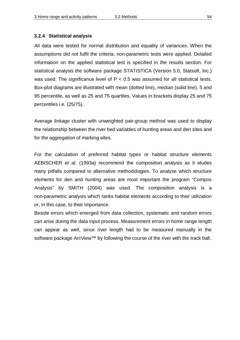
3 Home range and activity patterns 3.2 Methods 54
3.2.4 Statistical analysis
All data were tested for normal distribution and equality of variances. When the
assumptions did not fulfil the criteria, non-parametric tests were applied. Detailed
information on the applied statistical test is specified in the results section. For
statistical analysis the software package STATISTICA (Version 5.0, Statsoft, Inc.)
was used. The significance level of P < 0.5 was assumed for all statistical tests.
Box-plot diagrams are illustrated with mean (dotted line), median (solid line), 5 and
95 percentile, as well as 25 and 75 quartiles. Values in brackets display 25 and 75
percentiles i.e. (25/75).
Average linkage cluster with unweighted pair-group method was used to display
the relationship between the river bed variables of hunting areas and den sites and
for the aggregation of marking sites.
For the calculation of preferred habitat types or habitat structure elements
AEBISCHER et al. (1993a) recommend the composition analysis as it eludes
many pitfalls compared to alternative methodologies. To analyse which structure
elements for den and hunting areas are most important the program “Compos
Analysis” by SMITH (2004) was used. The composition analysis is a
non-parametric analysis which ranks habitat elements according to their utilization
or, in this case, to their importance.
Beside errors which emerged from data collection, systematic and random errors
can arise during the data input process. Measurement errors in home range length
can appear as well, since river length had to be measured manually in the
software package ArcView™ by following the course of the river with the track ball.

3 Home range and activity patterns 3.3 Results 55
3.3 Results
3.3.1 Home Range
3.3.1.1 Accessibility
The area in which the home range of the southern river otter was studied was not
of a homogeneous shape. Therefore there was not equal accessibility to locations
within this study area (Tab. 3.3.1). Less time was generally spent searching for
animals whose home range was more accessible by car. Besides animal F 03/36,
which occupied an area which was not possible to access at night due to the
danger of rocks, steep hills and deep canyons, all other home ranges were
accessible by car or by foot at any time.
Tab. 3.3.1: Accessibility of home ranges of three otters
ID Total Range MCP 100 (m.)
Possible by car (m) % only by foot
(m) % not possible at night (m) %
F 03/36 16894 9118 53.97 7776 46.03 4629 27.40
F 04/54 18663 14348 76.88 4315 23.12 -- --
M 04/40 17608 7075 40.18 10533 59.82 -- --
The average time spent to initially locate an animal was 1:58 hours
(SD = 1.44 min) (Tab. 3.3.2). Most of the home range of M 04/40 was only
accessible by foot and therefore most search time was spent on this animal (00:30
h – 11:30 h), followed by F 03/36 and F 04/54.
Tab. 3.3.2: Time spent for first location on animal
General positive search negative search ID Average
(hh:mm) Range
(hh:mm) Average (hh:mm)
Range (hh:mm)
Average (hh:mm)
Range (hh:mm)
F 03/36 02:38 00:24 – 06:30 02:00 00:24 –
05:30 04:41 03:00 – 08:00
F 04/54 02:18 00:50 – 04:05 01:57 00:50 –
03:50 03:26 02:10 – 04:05
M 04/40 03:48 00:30 – 11:30 01:57 00:30 –
08:20 05:30 01:00 – 11:30
Average 02:55 01:58 04:32
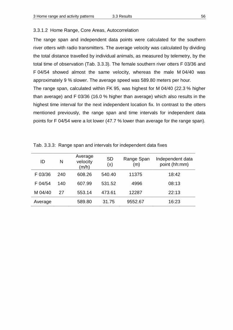
3 Home range and activity patterns 3.3 Results 56
3.3.1.2 Home Range, Core Areas, Autocorrelation
The range span and independent data points were calculated for the southern
river otters with radio transmitters. The average velocity was calculated by dividing
the total distance travelled by individual animals, as measured by telemetry, by the
total time of observation (Tab. 3.3.3). The female southern river otters F 03/36 and
F 04/54 showed almost the same velocity, whereas the male M 04/40 was
approximately 9 % slower. The average speed was 589.80 meters per hour.
The range span, calculated within FK 95, was highest for M 04/40 (22.3 % higher
than average) and F 03/36 (16.0 % higher than average) which also results in the
highest time interval for the next independent location fix. In contrast to the otters
mentioned previously, the range span and time intervals for independent data
points for F 04/54 were a lot lower (47.7 % lower than average for the range span).
Tab. 3.3.3: Range span and intervals for independent data fixes
ID
N
Average velocity (m/h)
SD (±)
Range Span (m)
Independent data point (hh:mm)
F 03/36 240 608.26 540.40 11375 18:42
F 04/54 140 607.99 531.52 4996 08:13
M 04/40 27 553.14 473.61 12287 22:13
Average 589.80 31.75 9552.67 16:23

3 Home range and activity patterns 3.3 Results 57
The manually calculated cumulative area curves for the two female (F 03/36;
F 04/54) and one male (M 04/40) radio tracked southern river otters illustrate
diverse rates of home range stabilisation (Fig. 3.3.1). Only the asymptotes for the
two females were attained. The fix number for range stabilisation for F 03/36 was
reached after 19 (and 59 respectively) and for female F 04/54 it was reached after
51 location fixes. Although the male southern river otter did not reach the
asymptote it was kept in calculations for comparison with data form literature.
Fig. 3.3.1: Kernel density asymptote analysis (FK 95) for three radio tracked southern river otters
Locations (n)
0 20 40 60 80
Riv
er le
ngth
(m)
0
2000
4000
6000
8000
10000
12000
14000
16000
F 03/36
Locations (n)
0 20 40 60 80
Riv
er le
ngth
(m)
0
2500
5000
7500
10000
12500
15000
17500
20000
F 04/54
Locations (n)
0 2 4 6 8 10 12 14
Riv
er le
ngth
(m)
0
5000
10000
15000
20000
M 04/40

3 Home range and activity patterns 3.3 Results 58
Total ranges (Fig. 3.3.2) were calculated for all three radio equipped southern river
otters using MCP 100 which includes all location fixes (Tab. 3.3.4). Home range
estimates were analysed by using MCP 95 and FK 95 and core areas were
measured using the minimum convex polygon and fixed kernel that includes 50 %
of location fixes (MCP 50, FK 50). Additional the core area with 25 % of location
fixes was quantified by using fixed kernel (FK 25) (Fig. 3.3.3; 3.3.4; 3.3.5).
MCP 95 and FK 95 were used as they are widely considered the best for home
range delineation (HARRIS et al., 1990; WHITE & GARROT, 1990) and the results
can be compared with data from the literature.
MCP 95 reduced the home range estimates by 20.0 % to 29.8 % compared with
MCP 100, whereas the reduction was lower in FK 95 (0.0 % to 15 %). Core area
estimates using MCP 50 represent a range form 6.6 % to 30.8 % of MCP 95 home
range areas. The fixed kernel core areas (FK 50) correspond to 5.4 % to 33.1 % of
FK 95 home range estimates. The additional home range with 25 % of
independent data fixes display approximately 7.7 % of FK 95 home range
estimates (range 5.4 % - 11.2 %). Although MCP and FK method display different
results, there was no significant disparity between the home ranges MCP 95 and
FK 95 or core areas MCP 50 and FK 50 (paired t-test: home ranges MCP/FK 95;
t = -2.454, P > 0.05; core areas MCP/FK 50; t = 0.161, P > 0.05).
Tab. 3.3.4: River length used by three southern river otters (total range, home range and core area)
Fixes Total range
(m)
Fixes Home range estimate
(m) Core area estimate
(m) Kernel h
factor ID
all
MCP 100
independent
MCP 95 FK 95
MCP 50 FK 50 FK 25
LSCV
F 03/36 2945
16894
68
13514 14358
4163 4749 1606
362
F 04/54 1558
18663
76
14397 17675
3594 3057 1165
241
M 04/40 663
17608
12
12365 17608
1162 952 952
608
Average
17722
13425 16547
2973 2919 1241
SD
890
832 1548
1594 1902 334
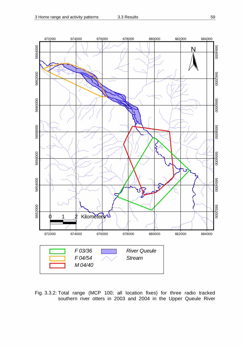
3 Home range and activity patterns 3.3 Results 59
N
0 1 2 Kilometers
672000
672000
674000
674000
676000
676000
678000
678000
680000
680000
682000
682000
684000
684000
5652
000 5652000
5654
000 5654000
5656
000 5656000
5658
000 5658000
5660
000 5660000
5662
000 5662000
5664
000 5664000
F 03/36F 04/54M 04/40
River QueuleStream
Fig. 3.3.2: Total range (MCP 100; all location fixes) for three radio tracked
southern river otters in 2003 and 2004 in the Upper Queule River
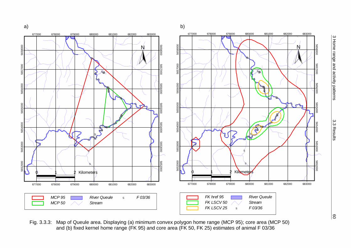
3 H
ome range and activity patterns
3.3 Results
60
#S
#S
#S
#S
#S
#S
#S
#S
#S
#S
#S
#S
#S
#S
#S
#S
#S
#S
#S
#S
#S
#S
#S
#S#S
#S
#S
#S
#S
#S
#S
#S
#S
#S#S
#S#S
#S
#S
#S
#S
#S
#S
#S
#S
#S
#S
#S
#S
#S
#S
#S
#S
#S
#S
#S#S
#S
#S
#S
#S
#S
#S
#S
#S
#S
#S
#S
N
0 1 2 Kilometers
677000
677000
678000
678000
679000
679000
680000
680000
681000
681000
682000
682000
683000
683000
5652
000 5652000
5653
000 5653000
5654
000 5654000
5655
000 5655000
5656
000 5656000
5657
000 5657000
5658
000 5658000
FK href 95FK LSCV 50FK LSCV 25
River QueuleStreamF 03/36 #S
#S
#S
#S
#S
#S
#S
#S
#S
#S
#S
#S
#S
#S
#S
#S
#S
#S
#S
#S
#S
#S
#S
#S
#S#S
#S
#S
#S
#S
#S
#S
#S
#S
#S#S
#S#S
#S
#S
#S
#S
#S
#S
#S
#S
#S
#S
#S
#S
#S
#S
#S
#S
#S
#S
#S#S
#S
#S
#S
#S
#S
#S
#S
#S
#S
#S
#S
N
0 1 2 Kilometers
677000
677000
678000
678000
679000
679000
680000
680000
681000
681000
682000
682000
683000
683000
5652
000 5652000
5653
000 5653000
5654
000 5654000
5655
000 5655000
5656
000 5656000
5657
000 5657000
5658
000 5658000
MCP 95MCP 50
River QueuleStream
F 03/36 #S
a) b) Fig. 3.3.3: Map of Queule area. Displaying (a) minimum convex polygon home range (MCP 95); core area (MCP 50)
and (b) fixed kernel home range (FK 95) and core area (FK 50, FK 25) estimates of animal F 03/36

3 H
ome range and activity patterns
3.3 Results
61
#S
#S#S
#S
#S#S#S
#S
#S #S
#S
#S
#S #S
#S #S#S
#S#S
#S
#S
#S
#S
#S#S
#S
#S
#S#S
#S
#S
#S#S
#S
#S#S
#S
#S
#S
#S#S
#S
#S
#S#S
#S#S
#S
#S
#S
#S#S
#S
#S
#S
#S
#S
#S
#S
#S#S
#S
#S
#S
#S
#S
#S
#S#S
#S
#S
#S
#S
#S
#S
#S
N
0 1 2 Kilometers
672000
672000
673000
673000
674000
674000
675000
675000
676000
6760005659
000 5659000
5660
000 5660000
5661
000 5661000
5662
000 5662000
5663
000 5663000
5664
000 5664000
MCP 95MCP 50
River QueuleStream
F 04/54#S
#S
#S#S
#S
#S#S#S
#S
#S #S
#S
#S
#S #S
#S #S#S
#S#S
#S
#S
#S
#S
#S#S
#S
#S
#S#S
#S
#S
#S#S
#S
#S#S
#S
#S
#S
#S#S
#S
#S
#S#S
#S#S
#S
#S
#S
#S#S
#S
#S
#S
#S
#S
#S
#S
#S#S
#S
#S
#S
#S
#S
#S
#S#S
#S
#S
#S
#S
#S
#S
#S
N
0 1 2 Kilometers
672000
672000
673000
673000
674000
674000
675000
675000
676000
6760005659
000 5659000
5660
000 5660000
5661
000 5661000
5662
000 5662000
5663
000 5663000
5664
000 5664000
FK href 95FK LSCV 50FK LSCV 25
River QueuleStreamF 04/54#S
a) b)
Fig. 3.3.4: Map of Queule area. Displaying (a) minimum convex polygon home range (MCP 95); core area (MCP 50) and
(b) fixed kernel home range (FK 95) and core area (FK 50, FK 25) estimates of animal F 04/54
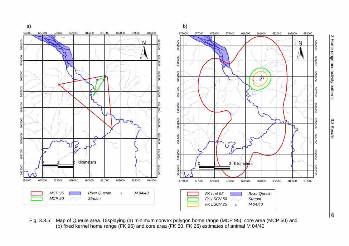
3 H
ome range and activity patterns
3.3 Results
62
#S
#S
#S
#S #S#S
#S#S
#S
#S
#S
#S
N
0 1 2 Kilometers
676000
676000
677000
677000
678000
678000
679000
679000
680000
680000
681000
681000
682000
682000
683000
683000
684000
684000
5652
000 5652000
5653
000 5653000
5654
000 5654000
5655
000 5655000
5656
000 5656000
5657
000 5657000
5658
000 5658000
5659
000 5659000
5660
000 5660000
MCP 95MCP 50
River QueuleStream
M 04/40#S
#S
#S
#S
#S #S#S
#S#S
#S
#S
#S
#S
N
0 1 2 Kilometers
676000
676000
677000
677000
678000
678000
679000
679000
680000
680000
681000
681000
682000
682000
683000
683000
684000
68400056
5200
0 5652000
5653
000 5653000
5654
000 5654000
5655
000 5655000
5656
000 5656000
5657
000 5657000
5658
000 5658000
5659
000 5659000
5660
000 5660000
FK href 95FK LSCV 50FK LSCV 25
River QueuleStreamM 04/40#S
b) a) Fig. 3.3.5: Map of Queule area. Displaying (a) minimum convex polygon home range (MCP 95); core area (MCP 50) and
(b) fixed kernel home range (FK 95) and core area (FK 50, FK 25) estimates of animal M 04/40

3 Home range and activity patterns 3.3 Results 63
3.3.2 Habitat preferences
3.3.2.1 Habitat composition of F 03/36
Habitat structure
< 15°
15° -
45°
> 45° 90
°
Sand,
Stone
Grass,
Herbs
Bushe
sTree
s
Big tre
esRoo
ts
Overha
nging
roots
Quila
Dead t
rees
Per
cent
age
com
posi
tion
0
10
20
30
40
50
Bank angleRiperian vegetation
Fig. 3.3.6: Habitat composition of the home range of female southern river otter
F 03/36. Mean values and standard errors for vegetation structure are shown (n=76)
As only the home range of F 03/36 was accessible, this home range was used for
examinations of habitat preferences.
Bank angles of >45 degrees (46.4 %) represent the most frequently occurring
riparian inclination followed by 90° bank angles (33.1 %) (Fig. 3.3.6). The
vegetation structure Grass/Herbs (38.2 %; SE = 2.59) is salient and is building a
group with the variables Bushes (29.2 %; SE = 2.37) and Sand/Stones (17.8 %;
SE = 2.24). The variables Trees and Quila are represented with 12.4 %
(SE = 1.86) and 7.5 % (SE = 2.51) respectively. Big trees (0.8 %; SE = 0.33),
Roots (0.66 %; SE = 0.16), Overhanging roots (1.2 %; SE = 0.30) and Dead trees
(0.1 %; SE = 0.10) occurred infrequently in the investigated home range of
F 03/36.
As the normality test failed the Kruskal-Wallis ANOVA on Ranks was performed.
The vegetation variables are significantly different (H= 361.734; df=8; p<0.001).
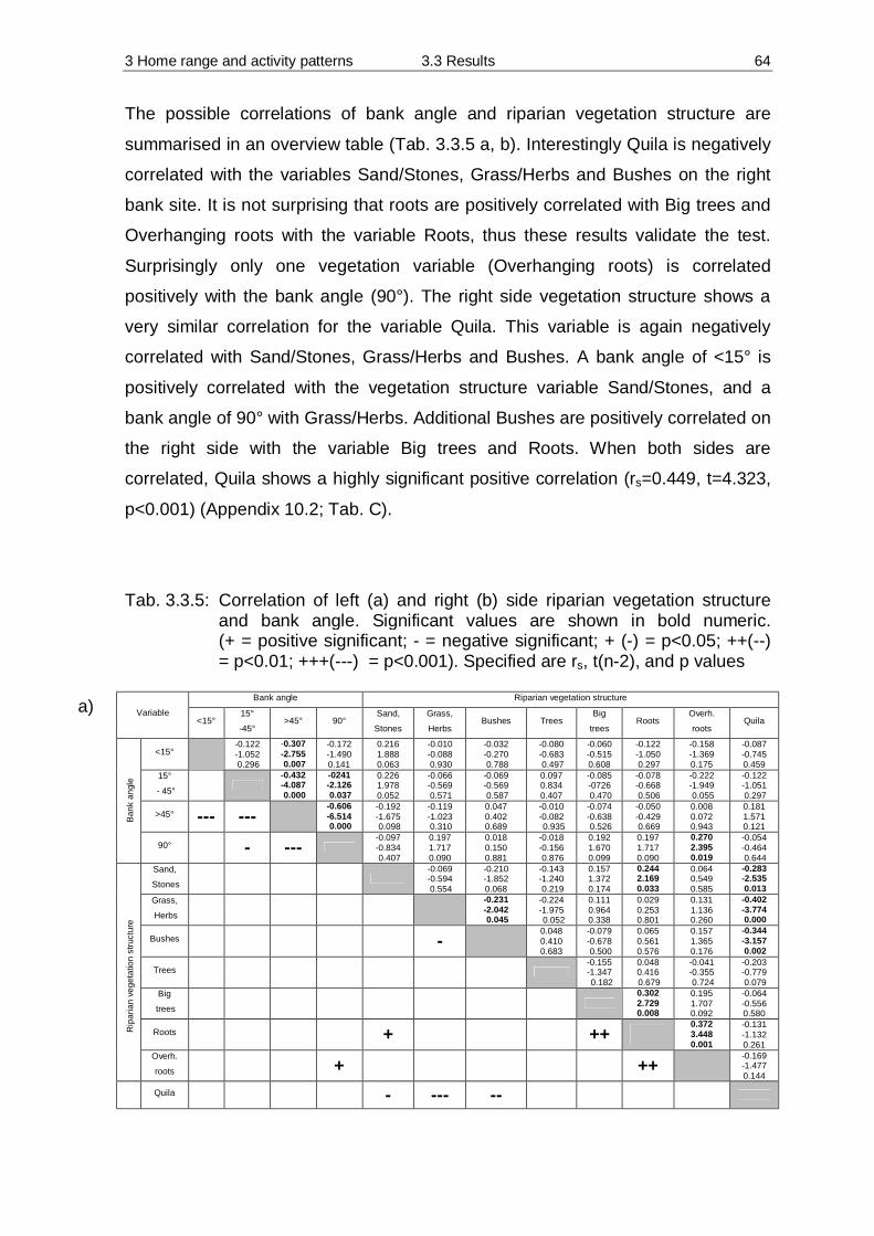
3 Home range and activity patterns 3.3 Results 64
The possible correlations of bank angle and riparian vegetation structure are
summarised in an overview table (Tab. 3.3.5 a, b). Interestingly Quila is negatively
correlated with the variables Sand/Stones, Grass/Herbs and Bushes on the right
bank site. It is not surprising that roots are positively correlated with Big trees and
Overhanging roots with the variable Roots, thus these results validate the test.
Surprisingly only one vegetation variable (Overhanging roots) is correlated
positively with the bank angle (90°). The right side vegetation structure shows a
very similar correlation for the variable Quila. This variable is again negatively
correlated with Sand/Stones, Grass/Herbs and Bushes. A bank angle of <15° is
positively correlated with the vegetation structure variable Sand/Stones, and a
bank angle of 90° with Grass/Herbs. Additional Bushes are positively correlated on
the right side with the variable Big trees and Roots. When both sides are
correlated, Quila shows a highly significant positive correlation (rs=0.449, t=4.323,
p<0.001) (Appendix 10.2; Tab. C).
Tab. 3.3.5: Correlation of left (a) and right (b) side riparian vegetation structure and bank angle. Significant values are shown in bold numeric. (+ = positive significant; - = negative significant; + (-) = p<0.05; ++(--) = p<0.01; +++(---) = p<0.001). Specified are rs, t(n-2), and p values
Bank angle Riparian vegetation structure
Variable <15°
15°
-45° >45° 90°
Sand,
Stones
Grass,
Herbs Bushes Trees
Big
trees Roots
Overh.
roots Quila
<15° -0.122 -1.052 0.296
-0.307 -2.755 0.007
-0.172 -1.490 0.141
0.216 1.888 0.063
-0.010 -0.088 0.930
-0.032 -0.270 0.788
-0.080 -0.683 0.497
-0.060 -0.515 0.608
-0.122 -1.050 0.297
-0.158 -1.369 0.175
-0.087 -0.745 0.459
15°
- 45° -0.432 -4.087 0.000
-0241 -2.126 0.037
0.226 1.978 0.052
-0.066 -0.569 0.571
-0.069 -0.569 0.587
0.097 0.834 0.407
-0.085 -0726 0.470
-0.078 -0.668 0.506
-0.222 -1.949 0.055
-0.122 -1.051 0.297
>45° --- --- -0.606 -6.514 0.000
-0.192 -1.675 0.098
-0.119 -1.023 0.310
0.047 0.402 0.689
-0.010 -0.082 0.935
-0.074 -0.638 0.526
-0.050 -0.429 0.669
0.008 0.072 0.943
0.181 1.571 0.121
Ban
k an
gle
90° - --- -0.097 -0.834 0.407
0.197 1.717 0.090
0.018 0.150 0.881
-0.018 -0.156 0.876
0.192 1.670 0.099
0.197 1.717 0.090
0.270 2.395 0.019
-0.054 -0.464 0.644
Sand,
Stones -0.069 -0.594 0.554
-0.210 -1.852 0.068
-0.143 -1.240 0.219
0.157 1.372 0.174
0.244 2.169 0.033
0.064 0.549 0.585
-0.283 -2.535 0.013
Grass,
Herbs -0.231 -2.042 0.045
-0.224 -1.975 0.052
0.111 0.964 0.338
0.029 0.253 0.801
0.131 1.136 0.260
-0.402 -3.774 0.000
Bushes - 0.048 0.410 0.683
-0.079 -0.678 0.500
0.065 0.561 0.576
0.157 1.365 0.176
-0.344 -3.157 0.002
Trees -0.155 -1.347 0.182
0.048 0.416 0.679
-0.041 -0.355 0.724
-0.203 -0.779 0.079
Big
trees 0.302 2.729 0.008
0.195 1.707 0.092
-0.064 -0.556 0.580
Roots + ++ 0.372 3.448 0.001
-0.131 -1.132 0.261
Rip
aria
n ve
geta
tion
stru
ctur
e
Overh.
roots + ++ -0.169 -1.477 0.144
Quila - --- --
a)
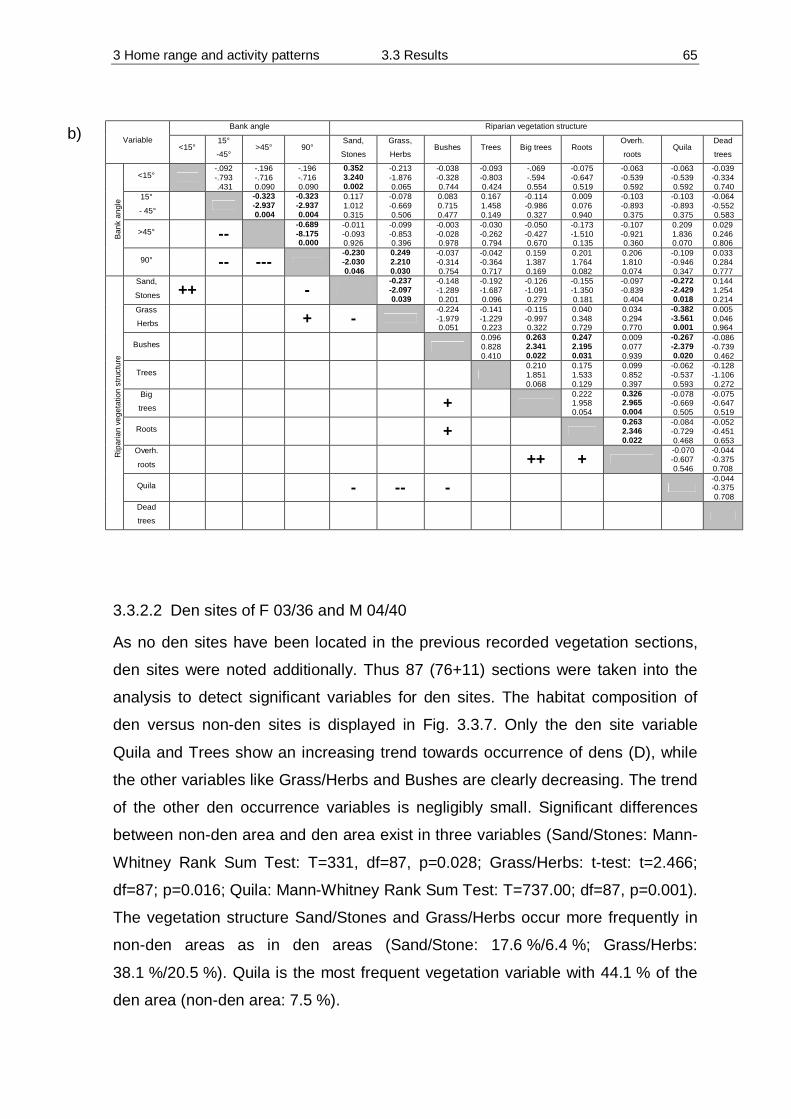
3 Home range and activity patterns 3.3 Results 65
3.3.2.2 Den sites of F 03/36 and M 04/40
As no den sites have been located in the previous recorded vegetation sections,
den sites were noted additionally. Thus 87 (76+11) sections were taken into the
analysis to detect significant variables for den sites. The habitat composition of
den versus non-den sites is displayed in Fig. 3.3.7. Only the den site variable
Quila and Trees show an increasing trend towards occurrence of dens (D), while
the other variables like Grass/Herbs and Bushes are clearly decreasing. The trend
of the other den occurrence variables is negligibly small. Significant differences
between non-den area and den area exist in three variables (Sand/Stones: Mann-
Whitney Rank Sum Test: T=331, df=87, p=0.028; Grass/Herbs: t-test: t=2.466;
df=87; p=0.016; Quila: Mann-Whitney Rank Sum Test: T=737.00; df=87, p=0.001).
The vegetation structure Sand/Stones and Grass/Herbs occur more frequently in
non-den areas as in den areas (Sand/Stone: 17.6 %/6.4 %; Grass/Herbs:
38.1 %/20.5 %). Quila is the most frequent vegetation variable with 44.1 % of the
den area (non-den area: 7.5 %).
Bank angle Riparian vegetation structure
Variable <15°
15°
-45° >45° 90°
Sand,
Stones
Grass,
Herbs Bushes Trees Big trees Roots
Overh.
roots Quila
Dead
trees
<15° -.092 -.793 .431
-.196 -.716
0.090
-.196 -.716 0.090
0.352 3.240 0.002
-0.213 -1.876 0.065
-0.038 -0.328 0.744
-0.093 -0.803 0.424
-.069 -.594
0.554
-0.075 -0.647 0.519
-0.063 -0.539 0.592
-0.063 -0.539 0.592
-0.039 -0.334 0.740
15°
- 45°
-0.323 -2.937 0.004
-0.323 -2.937 0.004
0.117 1.012 0.315
-0.078 -0.669 0.506
0.083 0.715 0.477
0.167 1.458 0.149
-0.114 -0.986 0.327
0.009 0.076 0.940
-0.103 -0.893 0.375
-0.103 -0.893 0.375
-0.064 -0.552 0.583
>45° -- -0.689 -8.175 0.000
-0.011 -0.093 0.926
-0.099 -0.853 0.396
-0.003 -0.028 0.978
-0.030 -0.262 0.794
-0.050 -0.427 0.670
-0.173 -1.510 0.135
-0.107 -0.921 0.360
0.209 1.836 0.070
0.029 0.246 0.806
Ban
k an
gle
90° -- --- -0.230 -2.030 0.046
0.249 2.210 0.030
-0.037 -0.314 0.754
-0.042 -0.364 0.717
0.159 1.387 0.169
0.201 1.764 0.082
0.206 1.810 0.074
-0.109 -0.946 0.347
0.033 0.284 0.777
Sand,
Stones ++ - -0.237 -2.097 0.039
-0.148 -1.289 0.201
-0.192 -1.687 0.096
-0.126 -1.091 0.279
-0.155 -1.350 0.181
-0.097 -0.839 0.404
-0.272 -2.429 0.018
0.144 1.254 0.214
Grass
Herbs + - -0.224 -1.979 0.051
-0.141 -1.229 0.223
-0.115 -0.997 0.322
0.040 0.348 0.729
0.034 0.294 0.770
-0.382 -3.561 0.001
0.005 0.046 0.964
Bushes 0.096 0.828 0.410
0.263 2.341 0.022
0.247 2.195 0.031
0.009 0.077 0.939
-0.267 -2.379 0.020
-0.086 -0.739 0.462
Trees
0.210 1.851 0.068
0.175 1.533 0.129
0.099 0.852 0.397
-0.062 -0.537 0.593
-0.128 -1.106 0.272
Big
trees
+ 0.222 1.958 0.054
0.326 2.965 0.004
-0.078 -0.669 0.505
-0.075 -0.647 0.519
Roots
+ 0.263 2.346 0.022
-0.084 -0.729 0.468
-0.052 -0.451 0.653
Overh.
roots
++ + -0.070 -0.607 0.546
-0.044 -0.375 0.708
Quila
- -- - -0.044 -0.375 0.708
Rip
aria
n ve
geta
tion
stru
ctur
e
Dead
trees
b)

3 Home range and activity patterns 3.3 Results 66
Vegetation structure
Sand/S
tones
Grass/H
erbs
Bushe
sTre
es
Big tre
esRoots
Overh
. roo
tsQuil
a
Dead tr
ees
Perc
enta
ge c
ompo
sitio
n
0
10
20
30
40
50
60
70Non-den areaDen area
*
*
***
Fig. 3.3.7: Percentage composition of non-den and den area variables. Mean values and standard errors are shown. * p< 0.05, ** p< 0.01, *** p< 0.001 (non-den area, n=76; den area, n=11)
Positive significant correlation between den vegetation variables exist for
Sand, Stone/Roots (rs=0.313, t=3.021, p=0.003) and Roots/Overhanging roots
(rs=0.251, t=2.39, p=0.02). The variable Quila shows a significant negative
correlation for four out of eight variables (Quila/Sand, Stones: rs=-0.468, t=-4.89,
p<0.001; Quila/Grass, Herbs: rs=-0.380, t=-3.78, p<0.001; Quila/Bushes:
rs=-0.400, t=-3.40, p<0.001; Quila/Overhanging roots: rs=-0.281, t=-2.70, p=0.008).
The dendogram (Fig. 3.3.8) displays the subsumption of the 87 riparian vegetation
sections. Only one cluster is of note in this figure, as it clearly demonstrates
correlation with the variables Overhanging roots, Roots, Dead trees, Big trees and
Trees. This cluster has a high Euclidean distance to the other variables. All other
variables create a cluster of their own.
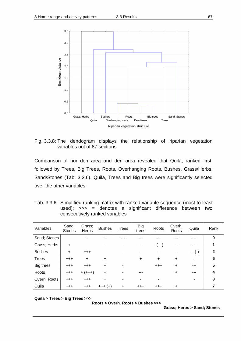
3 Home range and activity patterns 3.3 Results 67
Grass; HerbsQuila
BushesOverhanging roots
RootsDead trees
Big treesTrees
Sand; Stones
Riperian vegetation structure
0,0
0,5
1,0
1,5
2,0
2,5
3,0
3,5
Euc
lidea
n di
stan
ce
Fig. 3.3.8: The dendogram displays the relationship of riparian vegetation
variables out of 87 sections
Comparison of non-den area and den area revealed that Quila, ranked first,
followed by Trees, Big Trees, Roots, Overhanging Roots, Bushes, Grass/Herbs,
Sand/Stones (Tab. 3.3.6). Quila, Trees and Big trees were significantly selected
over the other variables.
Tab. 3.3.6: Simplified ranking matrix with ranked variable sequence (most to least used); >>> = denotes a significant difference between two consecutively ranked variables
Variables Sand; Stones
Grass; Herbs Bushes Trees Big
trees Roots Overh. Roots Quila Rank
Sand; Stones - - --- --- --- --- --- 0 Grass; Herbs + --- - --- - (---) --- --- 1 Bushes + +++ - - - - --- (-) 2 Trees +++ + + + + + - 6 Big trees +++ +++ + - +++ + --- 5 Roots +++ + (+++) + - --- + --- 4 Overh. Roots +++ +++ + - - - - 3 Quila +++ +++ +++ (+) + +++ +++ + 7
Quila > Trees > Big Trees >>> Roots > Overh. Roots > Bushes >>> Grass; Herbs > Sand; Stones

3 Home range and activity patterns 3.3 Results 68
3.3.2.3 Hunting Area
Most of the river bed structure variables of the investigated hunting areas are
influenced by river current, river width and river depth, only the variable woody
debris does not show any significant correlation to the river properties (Tab. 3.3.7).
Tab. 3.3.7: Correlation of river properties and river bed structures. Significant values are shown in bold numeric
River bed structure
Variable Sand Gravel Stones Rocks Woody debris
Current -0.402 -3.703 0.000
0.145 1.238 0.220
0.209 0.928 0.356
0.124 1.052 0.296
-0.004 -0.033 0.974
Width 0.268 2.374 0.020
-0.045 -0.389 0.699
-0.282 -2.516 0.014
-0.242 -2.239 0.037
0.130 1.119 0.267
Riv
er p
rope
rties
Depth 0.295 2.642 0.010
-0.419 -3.943 0.000
-0.232 -2.042 0.045
-0.184 -1.595 0.115
0.064 0.552 0.583
Out of 76 investigated sections, 18 were recorded as hunting areas as a result of
radio tracking sessions. The river bed composition divided into non-hunting and
hunting area is displayed in Fig. 3.3.9. The most recorded variable in the
non-hunting sections is sand with 46 %. All other variables have been smaller than
25 %. The hunting area is also dominated by the variable Sand (42 %). However,
Woody debris also plays an important role (40.3 %). While the variables for Sand,
Gravel, Stones and Rocks declines towards the hunting area (H), only the variable
Woody debris increases. A significant difference between non-hunting and hunting
area was found for Stones and Woody debris (Mann-Whitney Rank Sum Test:
Stones T = 496.00, p=0.016; Woody debris: T=1056.00, p<0.001). No statistically
significant differences were found for the variables river current, river width and
depth between non-hunting and hunting areas, (Mann-Whitney Rank Sum Test:
Current: T=814.50, df=75 p=0.676; Width: T=901.50, df=76, p=0.593; Depth:
T=838.00, df=76, p=0.942).
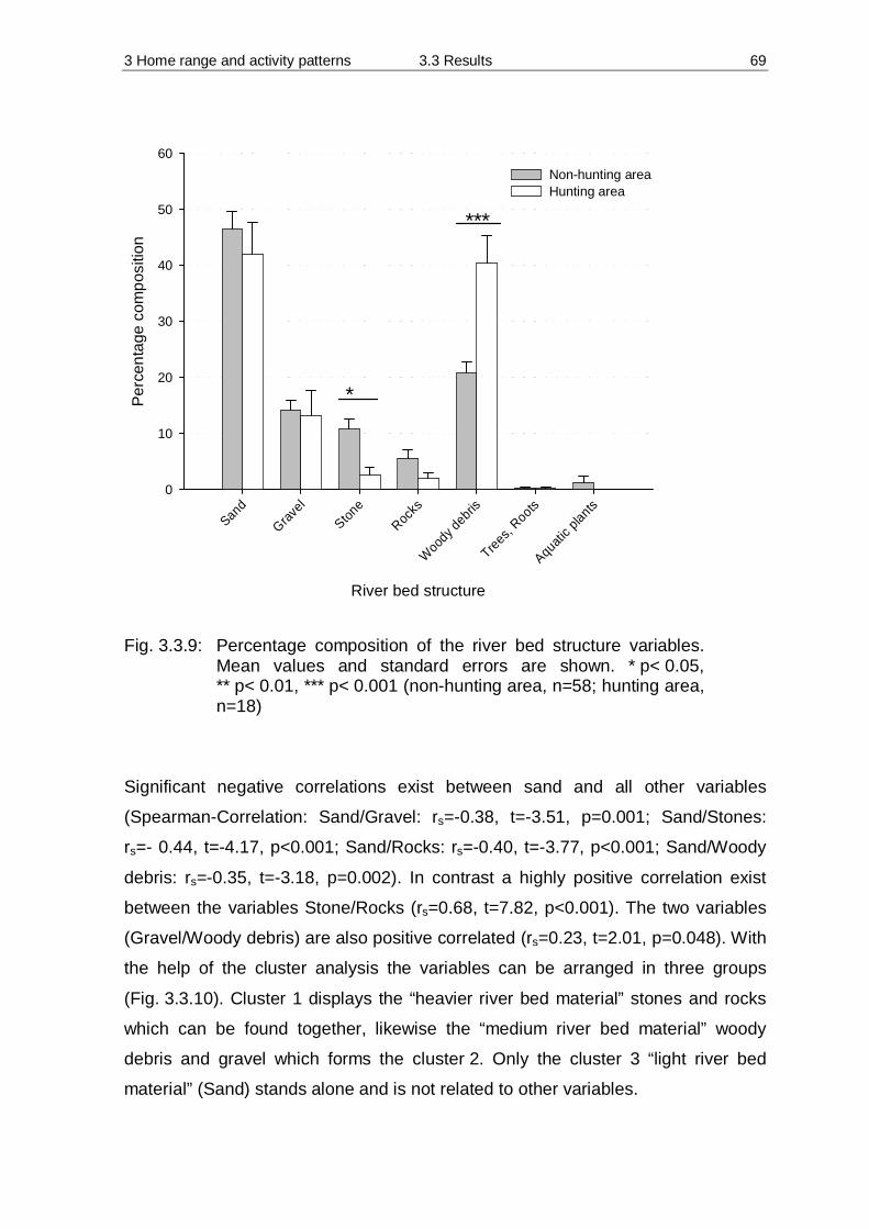
3 Home range and activity patterns 3.3 Results 69
River bed structure
Sand
Gravel
Stone
Rocks
Woody d
ebris
Trees, Roots
Aquatic p
lants
Per
cent
age
com
posi
tion
0
10
20
30
40
50
60Non-hunting areaHunting area
*
***
Fig. 3.3.9: Percentage composition of the river bed structure variables.
Mean values and standard errors are shown. * p< 0.05, ** p< 0.01, *** p< 0.001 (non-hunting area, n=58; hunting area, n=18)
Significant negative correlations exist between sand and all other variables
(Spearman-Correlation: Sand/Gravel: rs=-0.38, t=-3.51, p=0.001; Sand/Stones:
rs=- 0.44, t=-4.17, p<0.001; Sand/Rocks: rs=-0.40, t=-3.77, p<0.001; Sand/Woody
debris: rs=-0.35, t=-3.18, p=0.002). In contrast a highly positive correlation exist
between the variables Stone/Rocks (rs=0.68, t=7.82, p<0.001). The two variables
(Gravel/Woody debris) are also positive correlated (rs=0.23, t=2.01, p=0.048). With
the help of the cluster analysis the variables can be arranged in three groups
(Fig. 3.3.10). Cluster 1 displays the “heavier river bed material” stones and rocks
which can be found together, likewise the “medium river bed material” woody
debris and gravel which forms the cluster 2. Only the cluster 3 “light river bed
material” (Sand) stands alone and is not related to other variables.

3 Home range and activity patterns 3.3 Results 70
Rocks Stones Woody debris Gravel Sand1,0
1,5
2,0
2,5
3,0
3,5
4,0
Euc
lidea
n di
stan
ce
River bed variables
Cluster 1 Cluster 2
Cluster 3
Fig. 3.3.10: The dendogram displays the relationship of river bed variables out of
76 river bed structure sections in three clusters. Cluster 1: heavy; Cluster 2: medium; Cluster 3: light river bed material
The composition analysis revealed that woody debris ranked first, followed by
sand, gravel, rocks and stones in hunting areas (Tab. 3.3.8). Woody debris was
significantly selected over the other variables.
Tab. 3.3.8: Simplified ranking matrix with ranked variable sequence (most to least used); >>> = denotes a significant difference between two consecutively ranked variables
Variables Sand Gravel Stones Rocks Woody debris Rank
Sand + +++ +++ --- (-) 3 Gravel - +++ +++ --- 2 Stones --- --- --- --- 0 Rocks --- --- +++ --- 1 Woody debris +++ (+) +++ +++ +++ 4
Woody debris >>> Sand > Gravel >>> Rocks >>> Stones

3 Home range and activity patterns 3.3 Results 71
3.3.2.4 Distance to human constructions
Figure 3.3.11 displays the home range, divided into 50 m sections, of southern
river otter F03/36 and its relationship to human constructions. 54.4 % of its home
range is located closer than 150 m to human constructions. Only 19.2 % is more
than 450 m away from human constructions. The section at a distance of
100 - 150 m was most frequently used (35.1 %), and the animal was found more
frequently during day time (20.3 %) than at night (14.9 %) in this section. The
animal was present in the first section (0 - 50 m) for 27.6 % of total time observed
(14.2 % at day and 13.4 % at night). The five sections from 200 - 450 m were used
for 26.4 % of the time and the farthest section was visited during day time for
8.5 % of the time and 1.6 % at night.
0
10
20
30
40
0 - 50
50 -
100
100 -
150
150 -
200
200 -
250
250 -
300
300 -
350
350 -
400
400 -
450
> 450
Distance to Human Constructions (m.)
% o
f hom
e ra
nge
Used at NightUsed at DayAvailable
Fig. 3.3.11: Home range versus used sections by F03/36
The home range of F04/54 was mainly located far from human constructions
(Fig. 3.3.12). The farthest section was used 53.1 %, with 31.2 % during the day
and 36.9 % at night. The section 0 - 350 m was only visited for 23.7 % of all time
monitored. This area was mainly used at night (15.4 %) in contrast to 5.2 % during
the day. The southern river otter F04/54 was never found in the first section which
was the closest to human constructions (0 - 50 m).

3 Home range and activity patterns 3.3 Results 72
0
10
20
30
40
50
60
70
80
0 - 50
50 - 1
00
100 -
150
150 -
200
200 -
250
250 -
300
300 -
350
350 -
400
400 -
450
> 45
0
Distance to Human Constructions (m.)
% o
f hom
e ra
nge
Used At NightUsed at DayAvailable
Fig. 3.3.12: Home range versus used sections by F04/54
48.0 % of the home range of M04/40 is located close to human constructions
(0 - 200 m), where the animal was observed for 54.6 % of its time, with 20.8 %
during the day and 33.8 % at night (Fig. 3.3.13). 14.6 % of the time the animal was
monitored in the section 300 - 350 m (daytime 2.5 %; night time 12.1 %). The
southern river otter M04/40 was monitored for 28.1 % of its time (15.9 % during
the day; 12.2 % at night) in the farthest section (> 450 m) which constitutes 27.2 %
of its home range.
0
10
20
30
40
0 - 50
50 -
100
100 -
150
150 -
200
200 -
250
250 -
300
300 -
350
350 -
400
400 -
450
> 450
Distance to Human Constructions (m.)
% o
f hom
e ra
nge
Used at NightUsed at DayAvailable
Fig. 3.3.13: Home range versus used sections by M04/40

3 Home range and activity patterns 3.3 Results 73
3.3.2.5 Marking site
Fig. 3.3.14 displays the averages for marking sites. The mean average for bank
angle was 46.3° (SE = 4.5). Spraints were deposited at an average height of
78.6 cm from water level (SE=14.1) and at a horizontal distance from the water
line of 68.7 cm (SE = 10.1). The vegetation Soil/Stone with a proportion of 60.7 %
(SE = 6.6), followed by Grass/Herbs with 28.9 % (SE = 6.4) were most present at
average marking sites. The vegetation variables Bushes, Trees, Big trees, Roots,
Overhanging roots and Dead trees were each present for less than 5 %.
. Composition of marking spot
Bank a
ngle
FW h FW
v
Soil/S
tone
Grass/H
erbs
Bushe
sTree
s
Big tre
esRoo
ts
Overh.
roots
Dead t
rees
Ang
le (°
) / D
ista
nce
(cm
)
0
20
40
60
80
100
Vege
tatio
n in
%0
20
40
60
80
100Distance to spraintBank angleVegetation
Fig. 3.3.14: Average composition of 36 marking spots. FW h = Horizontal distance of faeces to water; FW v = Vertical distance of faeces to water
A positive significant correlation exists between the variable ‘horizontal distance of
faeces to water/vertical distance of faeces to water’ (FWh/FWv: rs=0.45, t=2.93,
p=0.006). The variables Soil, Stone/Grass, Herbs are negatively correlated
(rs=-0.86, t=-9.71, p<0.001). With the help of the cluster analysis the 36 mapped
sections were summarised in groups, which are characterised by special
combinations of structure variables (Fig. 3.3.15). In general two clusters, displayed
as cluster 1 and cluster 2, with a high Euclidean distance can be noted.
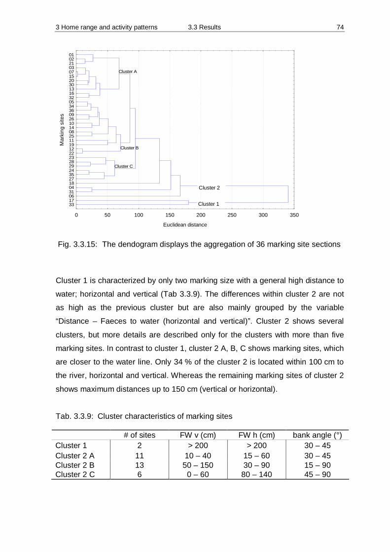
3 Home range and activity patterns 3.3 Results 74
0 50 100 150 200 250 300 350
Euclidean distance
331706310418273524292823221219112508141026093634053216133020150703210201
Mar
king
site
s
Cluster 1
Cluster 2
Cluster A
Cluster C
Cluster B
Fig. 3.3.15: The dendogram displays the aggregation of 36 marking site sections
Cluster 1 is characterized by only two marking size with a general high distance to
water; horizontal and vertical (Tab 3.3.9). The differences within cluster 2 are not
as high as the previous cluster but are also mainly grouped by the variable
“Distance – Faeces to water (horizontal and vertical)”. Cluster 2 shows several
clusters, but more details are described only for the clusters with more than five
marking sites. In contrast to cluster 1, cluster 2 A, B, C shows marking sites, which
are closer to the water line. Only 34 % of the cluster 2 is located within 100 cm to
the river, horizontal and vertical. Whereas the remaining marking sites of cluster 2
shows maximum distances up to 150 cm (vertical or horizontal).
Tab. 3.3.9: Cluster characteristics of marking sites # of sites FW v (cm) FW h (cm) bank angle (°) Cluster 1 2 > 200 > 200 30 – 45 Cluster 2 A 11 10 – 40 15 – 60 30 – 45 Cluster 2 B 13 50 – 150 30 – 90 15 – 90 Cluster 2 C 6 0 – 60 80 – 140 45 – 90
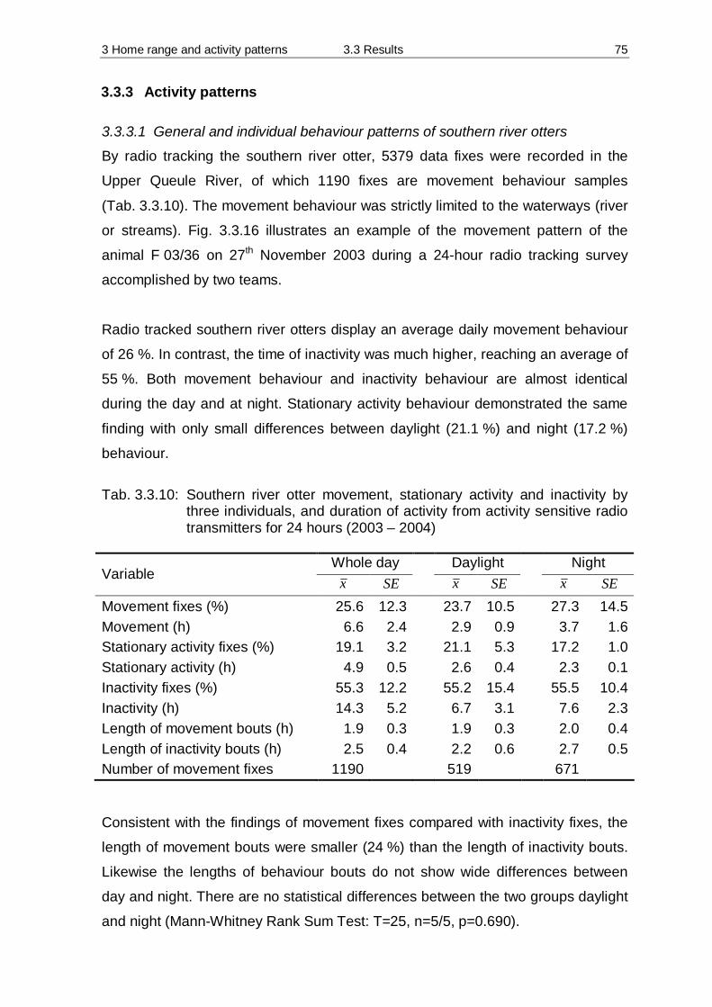
3 Home range and activity patterns 3.3 Results 75
3.3.3 Activity patterns
3.3.3.1 General and individual behaviour patterns of southern river otters
By radio tracking the southern river otter, 5379 data fixes were recorded in the
Upper Queule River, of which 1190 fixes are movement behaviour samples
(Tab. 3.3.10). The movement behaviour was strictly limited to the waterways (river
or streams). Fig. 3.3.16 illustrates an example of the movement pattern of the
animal F 03/36 on 27th November 2003 during a 24-hour radio tracking survey
accomplished by two teams.
Radio tracked southern river otters display an average daily movement behaviour
of 26 %. In contrast, the time of inactivity was much higher, reaching an average of
55 %. Both movement behaviour and inactivity behaviour are almost identical
during the day and at night. Stationary activity behaviour demonstrated the same
finding with only small differences between daylight (21.1 %) and night (17.2 %)
behaviour.
Tab. 3.3.10: Southern river otter movement, stationary activity and inactivity by
three individuals, and duration of activity from activity sensitive radio transmitters for 24 hours (2003 – 2004)
Whole day Daylight Night
Variable x SE x SE x SE Movement fixes (%) 25.6 12.3 23.7 10.5 27.3 14.5 Movement (h) 6.6 2.4 2.9 0.9 3.7 1.6 Stationary activity fixes (%) 19.1 3.2 21.1 5.3 17.2 1.0 Stationary activity (h) 4.9 0.5 2.6 0.4 2.3 0.1 Inactivity fixes (%) 55.3 12.2 55.2 15.4 55.5 10.4 Inactivity (h) 14.3 5.2 6.7 3.1 7.6 2.3 Length of movement bouts (h) 1.9 0.3 1.9 0.3 2.0 0.4 Length of inactivity bouts (h) 2.5 0.4 2.2 0.6 2.7 0.5 Number of movement fixes 1190 519 671 Consistent with the findings of movement fixes compared with inactivity fixes, the
length of movement bouts were smaller (24 %) than the length of inactivity bouts.
Likewise the lengths of behaviour bouts do not show wide differences between
day and night. There are no statistical differences between the two groups daylight
and night (Mann-Whitney Rank Sum Test: T=25, n=5/5, p=0.690).

3 Home range and activity patterns 3.3 Results 76
#
#
#
#
#
#
#######
#
###
#
######################
##
#
#
##
###
44
4345
46
47 - 49 4241
1
2
34
5
186
14
#7 - 13 #
19 - 40
# 171516
679500
679500
680000
680000
680500
680500
681000
681000
681500
681500
682000
682000
5654500 5654500
5655000 5655000
5655500 5655500
5656000 5656000
5656500 5656500
Time of fixes: 1: 00:00 12: 05:30 23: 11:00 34: 16:30 45: 22:00 2: 00:30 13: 06:00 24: 11:30 35: 17:00 46: 22:30 3: 01:00 14: 06:30 25: 12:00 36: 17:30 47: 23:00 4: 01:30 15: 07:00 26: 12:30 37: 18:00 48: 23:30 5: 02:00 16: 07:30 27: 13:00 38: 18:30 49: 00:00 6: 02:30 17: 08:00 28: 13:30 39: 19:00 7: 03:00 18: 08:30 29: 14:00 40: 19:30 8: 03:30 19: 09:00 30: 14:30 41: 20:00 9: 04:00 20: 09:30 31: 15:00 42: 20:30 10: 04:30 21: 10:00 32: 15:30 43: 21:00 11: 05:00 22: 10:30 33: 16:00 44: 21:30 Fig. 3.3.16: Movement behaviour and distances travelled by southern river otter
F 03/36 during a 24-hour radio tracking on 27th November 2003. Movement fixes are highlighted bold numerals in the table
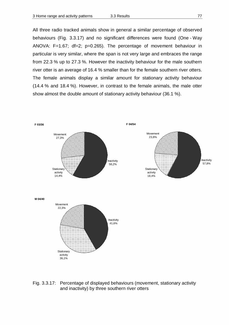
3 Home range and activity patterns 3.3 Results 77
F 03/36
Inactivity58,2%
Stationary activity14,4%
Movement27,3%
M 04/40
Inactivity41,6%
Stationary activity36,1%
Movement22,3%
F 04/54
Inactivity57,8%
Stationary activity18,4%
Movement23,8%
All three radio tracked animals show in general a similar percentage of observed
behaviours (Fig. 3.3.17) and no significant differences were found (One - Way
ANOVA: F=1.67; df=2; p=0.265). The percentage of movement behaviour in
particular is very similar, where the span is not very large and embraces the range
from 22.3 % up to 27.3 %. However the inactivity behaviour for the male southern
river otter is an average of 16.4 % smaller than for the female southern river otters.
The female animals display a similar amount for stationary activity behaviour
(14.4 % and 18.4 %). However, in contrast to the female animals, the male otter
show almost the double amount of stationary activity behaviour (36.1 %).
Fig. 3.3.17: Percentage of displayed behaviours (movement, stationary activity
and inactivity) by three southern river otters

3 Home range and activity patterns 3.3 Results 78
Movement behaviour was recorded throughout the 24 hour period during the radio
tracking study. However, the average distribution of movement behaviour was
uneven. Between 00:00 – 03:00 (30.3 %), 06:00 – 12:00 (32.0 %; 28.8 %) and
18:00 – 21:00 (32.5 %) the southern river otters showed more activity than during
the early morning 03:00 – 06:00 (19.8 %), afternoon 15:00 – 18:00 (17.4 %) and
21:00 – 24:00 (23.0 %) time periods (Fig. 3.3.18). Remarkably, the southern river
otters’ movement behaviour from 03:00 - 09:00 hours corresponds to
15:00 - 21:00 hours.
0
5
10
15
20
25
30
35
00-03 03-06 06-09 09-12 12-15 15-18 18-21 21-24
Time of day
Mov
emen
t
Fig. 3.3.18: Distribution of the average daily movement behaviour of three southern river otters throughout 24 h radio tracking (divided into 3-hour intervals)
The time an individual is sheltering in den or stayed out of the den in a 24-hour
cycle is displayed in Figure 3.3.19. The female southern river otter spent 67 % of
its time in a den; this finding is almost similar to the female animal F 04/54 which
stayed in den for 62 % of its radio tracked time. The male southern river otter
M 04/40 sheltered for the highest proportion of time in den (73 %). On average,
the observed animals shelter in their dens for most of the time ( %3.67=x ) and
have been recorded outside of den for only 32.7 %.

3 Home range and activity patterns 3.3 Results 79
0
25
50
75
100
F 03/36 F 04/54 M 04/40
Animals
% o
f tim
e
Outside of denSheltering in den
Fig. 3.3.19: Percentage of time radio tracked southern river otter spent sheltering
in den or outside of den
Regardless of time of day or night all types of behaviour were displayed
(Fig. 3.3.20). Only small and no significant variation in the proportion of daylight
and night behaviour occurred in the individual animal (t=-0.591, df=16, p=0.563).
33
2216
8 1016
11 13 10
25
36
25
69
20
16 1113
0
10
20
30
40
50
60
F03/36
F04/54
M04/40
F03/36
F04/54
M04/40
F03/36
F04/54
M04/40
Animal Behaviour
Per
cent
age
NightDay
Inactivity MovementStationary activity
Fig. 3.3.20: Frequency distribution of inactivity, stationary activity and movement behaviour of all fixes on radio tracked animals during day and night
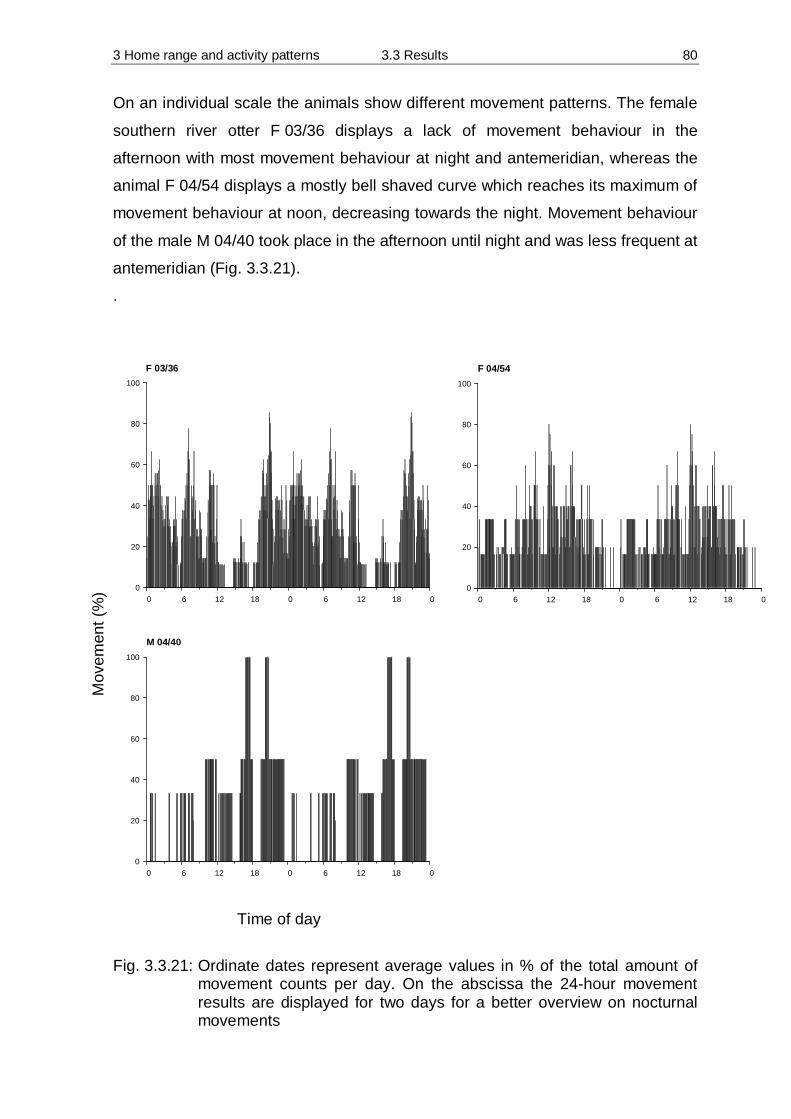
3 Home range and activity patterns 3.3 Results 80
On an individual scale the animals show different movement patterns. The female
southern river otter F 03/36 displays a lack of movement behaviour in the
afternoon with most movement behaviour at night and antemeridian, whereas the
animal F 04/54 displays a mostly bell shaved curve which reaches its maximum of
movement behaviour at noon, decreasing towards the night. Movement behaviour
of the male M 04/40 took place in the afternoon until night and was less frequent at
antemeridian (Fig. 3.3.21).
.
Fig. 3.3.21: Ordinate dates represent average values in % of the total amount of
movement counts per day. On the abscissa the 24-hour movement results are displayed for two days for a better overview on nocturnal movements
Time of day
Mov
emen
t (%
) 0 6 12 18 0 6 12 18 00
20
40
60
80
100
F 03/36
0 6 12 18 0 6 12 18 00
20
40
60
80
100
M 04/40
0 6 12 18 0 6 12 18 00
20
40
60
80
100
F 04/54
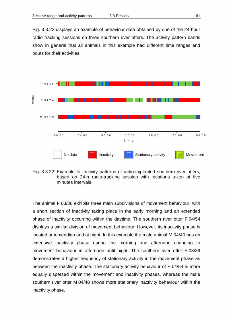
3 Home range and activity patterns 3.3 Results 81
Fig. 3.3.22 displays an example of behaviour data obtained by one of the 24-hour
radio tracking sessions on three southern river otters. The activity pattern bands
show in general that all animals in this example had different time ranges and
bouts for their activities.
Fig. 3.3.22: Example for activity patterns of radio-implanted southern river otters, based on 24-h radio-tracking session with locations taken at five minutes intervals
The animal F 03/36 exhibits three main subdivisions of movement behaviour, with
a short section of inactivity taking place in the early morning and an extended
phase of inactivity occurring within the daytime. The southern river otter F 04/54
displays a similar division of movement behaviour. However, its inactivity phase is
located antemeridian and at night. In this example the male animal M 04/40 has an
extensive inactivity phase during the morning and afternoon changing to
movement behaviour in afternoon until night. The southern river otter F 03/36
demonstrates a higher frequency of stationary activity in the movement phase as
between the inactivity phase. The stationary activity behaviour of F 04/54 is more
equally dispersed within the movement and inactivity phases, whereas the male
southern river otter M 04/40 shows more stationary inactivity behaviour within the
inactivity phase.
T i m e
0 0 : 0 0 0 4 : 0 0 0 8 : 0 0 1 2 : 0 0 1 6 : 0 0 2 0 : 0 0 0 0 : 0 0
Ani
mal
M 0 4 / 4 0
F 0 4 / 5 4
F 0 3 / 3 6
No data Inactivity Stationary activity Movement

3 Home range and activity patterns 3.3 Results 82
3.3.3.2 Movements and distance travelled
The travelled distance between inactive periods for all southern river otters is
shown in Figure 3.3.23 and averages 913.7 meters, with the mean of 664.1 m,
being lowest for F 03/36 ( )1.1089/8.134;4.248~ =x , followed by F 04/54 with
1383.6 m ( )1.2077/3.612;1.1287~ =x , having travelled more than twice the average
distance than F 03/36.
Animals
F 03/36 F 04/54 M 04/40
Dis
tanc
e (m
.)
0
500
1000
1500
2000
2500
3000
Fig. 3.3.23: Distance travelled by individual animals between inactive phases
The male southern river otter M 04/40 travelled almost the same distances as
F 04/40 (1235.1 m), with the median being 2.1060~ =x (134.8/1089.1).The
Kruskal-Wallis One Way Analysis of Variance on Ranks resulted in no significant
differences between the individuals (H=5; df=2; p=0.082).
The longest uninterrupted time of movement behaviour was observed in the
female F 04/54 (5.7 hours). The mean time for movement behaviour is lowest for
F 03/36 with 1.8 hours ( 46.2/88.0;78.1~ =x ). The time for movement behaviour for
F 04/54 averages 3.2 hours ( 58.4/92.1;75.2~ =x ), which is similar to the time of
movement behaviour noted for M 04/40 ( 42.4/60.1;42.2~;9.2 == xx hours )
(Fig. 3.3.24).

3 Home range and activity patterns 3.3 Results 83
Animals
F 03/36 F 04/54 M 04/40
Tim
e (h
.)
0
1
2
3
4
5
6
7
A B A,B
Fig. 3.3.24: Time range of movement per 24h; same letter per animals = no
significant difference; different letter per animal = significant difference
ANOVA was performed and a significant difference between the times of
movement behaviour was found (H=7.24; df=2; p=0.027). The subsequent
pairwise multiple comparison procedures (Dunn’s Method) show a statistical
difference between F 03/36 and M 04/40 (Difference of Ranks = 9.8; Q=2.6;
p<0.05). The average movement velocity and maximum velocity a southern river
otter swam during the study period was highest for female F 04/54 with 1.59 km/h
and 12.70 km/h respectively (Tab. 3.3.11).
Tab. 3.3.11: Calculated velocity of radio tracked southern river otter
Velocity (km/h) ID x SE
Maximum velocity (km/h)
F 03/36 1.08 0.05 11.25 F 04/54 1.59 0.10 12.70 M 04/40 1.24 0.10 6.28
Average ( x ) 1.49 0.05 10.08
3 Home range and activity patterns 3.4 Discussion 84
3.4 Discussion
A significant part of the present research looked at the animals’ habitat use and
preference of an area, as well as the amount of time the southern river otter spent
on different activities. It would not be possible to make a meaningful statement as
to whether the southern river otter has special habitat requirements or shows a
typical circadian cycle without the information about home range, activity patterns
and habitat preferences.
3.4.1 Methodology
Telemetry
Animals such as Lontra provocax are extremely difficult to study by direct
observation alone because of their shyness, and due to their agile movements.
Tracking animals which have a transmitter is therefore a useful technique to find
out about the activity patterns, behaviour, habitat use and movements of these
animals or about animals in general. Furthermore conclusions regarding habitat
preference can be drawn (WHITE & GARROT, 1990).
The first use of wildlife transmitters was on heart rates on chipmunks in 1959 by
LE MUNYAN (1959). Later studies on radio tracking have been conducted
primarily on terrestrial animals due to the problem of attaching the transmitter to an
aquatic or semi-aquatic animal. On otters, especially Lutra lutra, several methods
to attach external radio transmitters have been attempted, including collars and
harness (GREEN et al., 1984), but these are problematic, not only because of the
high danger they pose the otter in getting it caught under water and causing it to
drown (MASON & MCDONALD, 1986), but also because of the difficulty in fitting
the collar as the neck of an otter is thicker than its head. Furthermore, the lifespan
of collar or harness is shortened by its frequent rubbing behaviour to keep its fur
dry and clean (HERNANDEZ-DIVERS et al., 2001). However, MELQUIST &
HORNOCKER (1979) developed implantable radio transmitters for otters, which
were used first on Lontra canadensis by implanting into the intraperitoneal cavity.
The surgery for implanting radio transmitters appears to be safe, as further
operations on Lontra canadensis (ERICKSON & MCCULLOUGH, 1987;
HERNANDEZ-DIVERS et al., 2001; HOOVER, 1984; POLECHLA, 1988), Enhydra
lutris (WILLIAMS & SINIFF, 1983) and on Lutra lutra (ARNEMO, 1990; RUIZ-

3 Home range and activity patterns 3.4 Discussion 85
OLMO et al., 1992) did not show significant problems. This is consistent with
observations on L. provocax in this study, as the female otter F 03/36 gave birth to
two cubs, even though she received the intraperitoneal radio transmitter
approximately 20 weeks before.
Two different methods can be used in radio tracking: 1) sequential and 2)
continuously tracking of radio equipped animals, which have advantages and
disadvantages. By using sequential tracking it is possible to locate several
different animals within a short time. Therefore it is possible to compare the
animals’ activity directly, as abiotic factors like temperature and precipitation,
which may change activity patterns, are equal. On the other hand, it is not possible
to accurately ascertain the actual time an animal spent travelling, resting or
feeding, or the travel distance or habitat preference.
In this study the accessibility to the areas and time spent on first location for radio
tracked southern river otters were different (Tab. 3.3.1; p. 55). Therefore the
results could show the investigators accessibility to an area rather than the
animal’s true home range, this bias is often ignored (MELQUIST & HORNOCKER,
1983). However, this kind of bias does not exist when focused on only one animal
by using the continuous tracking method. It is assumed that a more realistic
description of spacing and activity patterns is possible using this method, as more
data points will be obtained and the investigator also can follow the animal in
areas which are difficult to access. However this method is time consuming and
the problem of data independence arises. Both methods were used in this study.
Continuous tracking was used primarily to obtain data for activity patterns and
sequential tracking was used to obtain additional data for the home range
estimation for L. provocax.
Two teams located the animal and noted the activity status in order to obtain data
regarding home range and activity patterns. Personal abilities may have, to a
certain degree, influenced the accuracy of telemetry and the identification of the
activity status. Furthermore technical problems occurred twice and may have
biased the radio tracking results in some respects. On one occasion solar winds
produced strong static noises causing a very weak radio tracking signal and it is
assumed that this resulted in some bearing errors; therefore this data was not
used. Furthermore the lifetime of the transmitter was shorter than declared and the

3 Home range and activity patterns 3.4 Discussion 86
transmitting signal stopped after 9 months instead of 12 months. Thus data
collection was not maintained over all seasons.
Bearing error
Bearing errors are caused by manifold aspects like terrain, observer, and physical
factors. In weald and plain landscape, errors on bearings for radio-tracked animals
are usually low, but dense vegetation and difficult terrain, like slopes, hills or
mountains, can produce systematic bearing errors by bouncing, bending and
refracting the radio waves, resulting in misinterpretation of the location of the
radio-tracked animal (SCHOBER, 1986; WHITE & GARROT, 1990). To reduce
this kind of error, bearings from multiple elevated locations were taken (GARROTT
et al., 1986). Roads and fields in the study area were mostly higher than the river
where the radio tracked animal occurred, but there were still difficulties in receiving
signals due to the complexity of the terrain. Furthermore, there were errors caused
by animal movement which resulted from the velocity and distance to the animal
(WHITE & GARROT, 1990).
Home Range estimation
The size and utilization of an animal's home range can be determined by analyses
of telemetry data (AEBISCHER et al., 1993b; HARRIS et al., 1990; KENWARD et
al., 2001; WHITE & GARROT, 1990). Numerous home-range models can be
found in the literature, which describe methods for defining the area used by an
animal. In general the available home range estimation programs can be classified
into two groups: (1) models that connect the area between locations and (2)
nonparametric models, which analyse the location density.
The minimum-convex-polygon (MOHR, 1947), and the minimum-concave-polygon
(HARVEY & BARBOUR, 1965) can both be placed in the former group. These
models are descriptive and non-statistical.
The second group of programs is based on location density, and includes the
harmonic mean (DIXON & CHAPMAN, 1980), Fourier series (ANDERSON, 1982),
bivariate normal (JENNRICH & TURNER, 1969), adaptive and fixed kernel
(WORTON, 1989), and the time-kernel (KATAJISTO & MOILANEN, 2006).
3 Home range and activity patterns 3.4 Discussion 87
The MCP (minimum-convex-polygon) is the most commonly used method for
describing the total area used by the animal as well as the overlapping of home
ranges (BELANT & FOLLMANN, 2002; HORNER & POWELL, 1990). Therefore
the MCP method is widely used for comparison on intra-studies.
Weaknesses of the MCP method include a lack of consideration for the density
distribution of the locations, sensitivity to sample sizes, and especially to outliers
far from the centre of activity (HARRIS et al., 1990; SEAMAN et al., 1999; WHITE
& GARROT, 1990). When the outer location sightings form a convex shape, then
the estimates are highly accurate since they do not include unused areas.
However, if the shape formed by the outer locations is not convex, then unused
areas, which normally do not form a part of the home range, will be incorporated
into the model and the resulting estimate will be too large (ANDERSON, 1982).
The kernel method uses a smoothing parameter (h), which is also referred to as
‘bandwidth’, or ‘smoothing width’, in order to improve the fit of the contours to the
data. As the value of the smoothing factor is increased, the accuracy of the fit onto
the samples decreases. According to SILVERMAN (1994), the adjustment settings
of the smoothing factor are the most important adjustments in the kernel method
because they have such a large influence on the results. There are two different
possible approaches for dealing with these adjustments: the fixed kernel model
and the adaptive kernel model. The fixed kernel method uses a single smoothing
factor for a given data set, and the adaptive kernel method calculates a new
smoothing factor for each area with a different density, such that the area with
fewer location fixes receive higher h values (e.g. greater smoothing) and areas
with a greater number of location fixes are calculated with a smaller h value
(SILVERMAN, 1994).
The smoothing factor can be derived by trial and error through multiple analyses,
where the best results are used (KERNOHAN et al., 2001). However, such a
selection is not statistically reliable. Two statistical methods are presented by the
reference method (WORTON, 1995) and the least squares cross validation
method (SILVERMAN, 1994). When using the reference method it is important to
bear in mind that this method is only optimal for bivariate normal distributions. As
home ranges are usually not normal distributed, they can be greatly overestimated
by using the reference method (SEAMAN et al., 1998). The least square cross

3 Home range and activity patterns 3.4 Discussion 88
validation method, on the other hand, is nearly free of bias. The nonparametric
fixed kernel method with least square cross validation is therefore considered to
be the best choice for unbiased home range estimation and therefore was used in
the present study (BELANT & FOLLMANN, 2002; SEAMAN et al., 1998; SEAMAN
& POWELL, 1996; WORTON, 1995). However, all these methods were developed
using animals that occupy a two-dimensional range (measured in square meters)
and can move without restraint anywhere in their landscape (BLUNDELL et al.,
2001). In contrast, otters often use linear home ranges (measured in meters),
which is bound to the course of a water way.
BLUNDELL et al. (2001) who evaluated the effects of smoothing parameter,
sample size and independences of data points on kernel estimates for linear home
ranges, suggested that fixed kernel href with 95 % contours for home range
provides more reliable and consistent estimates and these were used in the
present study.
Core Areas
To evaluate the use of habitat within the home range, it is necessary to calculate
the use of space (BELANT & FOLLMANN, 2002). Because resources are normally
not homogenously distributed in an area, but rather occur in clumps, the area used
by the animal is usually heterogeneous. The area within the home range, which
contains a higher activity or density of locations, is termed the core area (SAMUEL
et al., 1985; WORTON, 1989). POWELL (2000) postulates that core areas are of
ecological importance because in these areas, which include breeding areas,
resting places and hunting areas, there is a higher accumulation of resources and
a higher density of nutrients than in peripheral areas. Therefore not all parts of a
home range are equally important for an individual.
The kernel method provides a good method for identifying and analysing core
areas, where a higher density of locations exist, (KENWARD et al., 2001) since
the utility distribution is displayed as percentage used areas with specified
probabilities (POWELL, 2000). However, it is assumed that for an assessment of
the habitat utilization, both the number of individuals and the number of locations
are required (OTIS & WHITE, 1999).
Core areas should not merely describe regions in which the animal is likely to be,
but rather should also be tested for biological meaning as regards the nature of the
3 Home range and activity patterns 3.4 Discussion 89
terrain, since this can sometimes indicate social interactions on an intra- and
interspecific level (HARRIS et al., 1990).
In several studies FK 50 and MCP 50 are used to describe core areas. However a
general conclusion towards which is the most suitable method is not possible as
MCP 50 in general does not show higher or lower values in relation to FK 50 in the
present study. Core area estimates by MCP 50 or FK 50 may not describe the real
core area, as they may overestimate the centre of activity in a linear system. Thus
river sections without any special features of ecological importance are included in
this study. By using FK 25 the core areas are reduced in length, but display the
more ecologically important areas, such as den areas, as supposed by POWELL
(2000).
Autocorrelation
Nonparametric models of home range, such as the kernel model, assume that the
locations used have been sampled independently (HARRIS et al., 1990). When
the time intervals between the location samples of the animal are too short, auto-
correlation occurs and the resulting data do not represent an independent fix of the
animal's movement and may instead be underestimated (SWIHART & SLADE,
1985; WORTON, 1989).
Several methods have been developed to verify the independence of data points
(SWIHART & SLADE, 1985). However, there are multiple methods available for
statistical analysis of autocorrelation and these can produce a wide range of
possible results leading to a variety of different interpretations.
An increase in the time intervals between location samples in order to achieve
statistical independence will most likely result in an underestimation of the home
range and a loss of biologically relevant information (ROONEY et al., 1998).
Furthermore, the independence of the data is affected by the biological conditions
(LAIR, 1987).
The independence of locations can also be calculated by the maximum distance
between two fixes within the home range, also know as “range span,” and the
average velocity. As a result, the location fixes will be interpreted as independent
when the time interval between two successive locations potentially allows an
animal to reach any location in his home range (SWIHART & SLADE, 1985;
WHITE & GARROT, 1990). Range span was calculated for all three animals.
3 Home range and activity patterns 3.4 Discussion 90
However, due to the different range span, particularly for F 04/54 the independent
data points between the three radio tracked southern river otters differed highly.
As the animal F 04/54 was situated in the ombrophilous swamp forest, where a lot
of streams were parallel and crosslinked, range span and time for independent
data points were smaller.
Beside the selection of the home range estimator, the selection of the software
program is important. A comparative study by LAWSON & RODGERS (1997)
pointed out that similar programs of home range estimation resulted in significant
differences concerning the size of the home range and the core areas.
3.4.2 Home Range
Fidelity to a specific home range is beneficial for individuals since they are familiar
with the local prey, resting sites, shelter, and mates. It also reduces competition for
resources (O´DOHERTY et al., 1997; mentioned in PAYER et al. 2004; POWELL,
1994). Furthermore, the risk of mortality is reduced since the animals are not
wandering into unknown habitats (THOMPSON & COLGAN, 1987).
Home range stabilisation and size
Both female southern river otter meet the asymptote for home range stabilization.
This is in contrast to the male individual. According to POWELL (1979), who
classifies individual mustelides into three groups: (1) 'transients', which are
animals who simply pass through an area; (2) 'temporary residents', which are
individuals who stay for a short period of time, and (3) 'residents', which stay for a
prolonged time or for their entire life in an area, the female southern river otter
should be classified as resident. The female F 03/36 feature more than one range
stabilisation. This is due to the different fixes found between the antenatal and
postnatal periods for this animal.
It is assumed that the female F 03/36 reached the asymptote earlier than F 04/54
since the home range of F 03/36 is more linear, having no interconnections
between streams as was the case for F 04/54. In the case of M 04/40 it seems that
the animal is a temporary resident, as it did not attain the asymptote and radio
contact was lost after four months of radio tracking. Furthermore, animal M 04/40

3 Home range and activity patterns 3.4 Discussion 91
was aged as a sub-adult and may have searched for an area to occupy in order to
establish its territory. However, taken into consideration must be the fact that the
transmitter was defective. The calculated data still can serve as an approximate
value for future research.
Home range size varied between female southern river otters. The estimated
home range for F 03/36 was 18.8 % smaller than the others. Finding intra-sexual
differences in home range sizes is consistent with previous studies on L. provocax
(SEPULVEDA TERÁN, 2003) , and was also reported for other species, such as
L. lutra (GREEN et al., 1984).
If the male home range is larger than that of females, it may be possible to
attribute this to the fact that the sub-adult male southern river otter M 04/40 is not
a resident animal. However, previous studies on male home ranges of L. provocax
show large variations (SEPULVEDA TERÁN, 2003).
The female F 03/36 was captured in 2000, 2002 and 2003 and equipped with a
radio transmitter. In 2000 the animal was classified as juvenile and the calculated
home range averaged 11298m (SEPULVEDA TERÁN, 2003). In 2002 the female
southern river otter already reached the adult status and occupied a home range
of 8922m (unpublished data). With data taken in 2003 a home range of 14358m
(FK 95) was calculated. However, by excluding the time were F 03/36 was
travelling with cubs, almost same home range size as recorded in 2002 was
estimate for the animal (FK 95 = 8490 m). As this female used always the same
upper section of the Queule River, it is assumed that she established its home
range most likely in 2000 and maintained it at least until end of November 2003
when last radio contact was recorded.
Factors influencing home range size
The size of home ranges depends on a multitude of factors; such as body size,
den sites, food resources and mating partners (e.g. GOMPPER & GITTLEMAN,
1991; HERFINDAL et al., 2005; POWELL, 1979).
MCNAB (1963) showed that home range size increases with metabolic needs, and
that it also varies with body mass (MACE & HARVEY, 1983). However, even in
animals with similar body weight, home ranges can vary by factors from 6 to 1400
(GITTLEMAN & HARVEY, 1982) . In this study, it was not possible to conclude
that there exists a relationship of body size to home range size because the

3 Home range and activity patterns 3.4 Discussion 92
number of radio- tracked otters was too low. Also, previous work on the home
ranges of the southern river otter does not provide sufficient data to make these
conclusions. However, as shown in Chapter 2, the sexual dimorphism in
L. provocax is low; therefore, an intra-specific difference, based on metabolic
needs, is not assumed for this species.
MCLOUGHLIN & FERGUSON (2000) suggest that home range size is primarily
related to prey availability and habitat productivity; and, therefore, home ranges
where there are fewer prey productive patches have to be larger in order to meet
individual needs. This relationship is also reported for different species, such as
mule deer Odocoileus hemionus crooki (RELYEA et al., 2000), red squirrels
Sciurius vulgaris (WAUTERS & DHONDT, 1992), red fox Vulpes vulpes
(LUCHERINI & LOVARI, 1996), Cape clawless otter Aonyx capensis, (SOMERS &
NEL, 2004) and northern river otter Lontra canadensis (BLUNDELL et al., 2000).
There is, however, a relationship between the home range size and prey
availability for the southern river otter that can be assumed, but is difficult to test
as the productive areas are too complicated to investigate. Thus, the results in this
study seem to have conflicting outcomes. F 04/54 has a home range area located
in the ombrophilous swamp forest. This is assumed to be a highly productive area,
but shows a higher FK 95 as F 03/36 where the patches of food were of lower
densities.
Seasonal changes in home range size during the mating season, and postnatally,
are known for several species; for example, the male brown bear Ursus arctos
(DAHLE & SWENSON, 2003), black-faced impalas Aepyceros melampus petersi
(MATSON et al., 2007) and stoats Mustela erminea (ERLINGE & SANDELL,
1986). A postnatal change in home range size was also noted for F 03/36, but is
discussed in detail in Chapter 4.
When a male otter die, its territorial vacancy has to be filled; and, sub-adult
animals may be the ones to occupy this area. POWELL (1979) noted that sub-
adult, L. lutra (two year old), showed territorial activity in the autumn; that is, they
seem to establish territories during this time. This may also be the case of
M 04/40; the animal was classified as a sub-adult and during the period of radio-
tracking it disappeared several times. This can be explained as a period of time
where the animal was surveying (travelling) in search of vacant territories. It is
assumed that temporary resident male southern river otters do not influence the
3 Home range and activity patterns 3.4 Discussion 93
spacing pattern of resident animals. This was also reported by HAWLEY &
NEWBY (1957; cited in POWELL 1979) for transients or temporary residents least
weasel Mustela nivalis.
Human disturbances are assumed to have influence on the home range size of
otters since they are altered environments (SOMERS & NEL, 2004). Most of the
F 03/36 home range was located close to human construction sites. However,
even within her home range there existed sections that were further away from
human construction areas. These areas were used less frequently, but they did
provide den and hunting sites. Furthermore, southern river otters were seen
swimming close to fishermen who were fishing in the river. They were also seen in
areas where the riparian trees had been cut with motor saws. (pers. obs.).
Therefore, it seems that the F 03/36 is, to a certain degree, tolerant to
anthropogenic disturbances such as those reported for the European otter,
Lutra lutra (KRUUK, 1995). It is possible, however, that the female southern river
otter had to choose a suboptimal habitat because no other habitat was available.
Animal F 04/54 shows a different activity pattern in relation to its distance from
human construction sites. Travelling through sections that were close to human
construction sites was carried out exclusively during the night time. The male
southern river otter M 04/40 seemed to avoid travelling during the day time
through sections which were close to human construction sites. This may be the
result of avoiding human activity and traffic that were highest during the day time.
Spacing pattern
Mustelides generally demonstrate intrasexual territoriality. However this is
determined by resources. For example, females occupy a home range that
provides enough prey in which to rear offspring, and males inhabit a home range
wherein they can maximize their reproductive success and is therefore only
partially influenced by prey availability (JOHNSON et al., 2000). However, there is
a wide variation in the spacing patterns within species. Thus, even though weasels
Mustela nivalis and stoats Mustela erminea have an intersexual and intrasexual
overlap of home ranges, there is spatio-temporal separation between and within
the sexes (ERLINGE, 1974; KING, 1975).
ERLINGE & SANDELL (1986) have shown that male Mustela erminea changed
home range size in response to competition with females over resources. The data

3 Home range and activity patterns 3.4 Discussion 94
on home range should therefore be related to the season during which they were
conducted (JOHNSON et al., 2000), particularly since habitat requirements can be
different in winter versus summer (BUSKIRK & LINDSTEDT, 1989).
Likewise, variation in spacing patterns and intrasexual territoriality has been
reported in the subfamily Lutrinae. For example, a strong intrasexual territoriality
has been described for the European otter Lutra lutra (ERLINGE, 1967, 1968,
mentioned in POWELL, 1979), whereas the northern river otter Lontra canadensis
does not show territoriality and there is an intra- and intersexual overlap of their
ranges (BOWYER et al., 1995; MELQUIST & HORNOCKER, 1983). The Cape
clawless otter Aonyx capensis spacing pattern seems to be similar to Lontra
canadensis, except that there is a temporal instead of spatial avoidance
(SOMERS & NEL, 2004; VAN DER ZEE, 1982). Although sea otters Enhydra lutris
normally exhibit intrasexual territoriality, during the breeding season adult males
occupy territories that overlap with female territories (ESTES, 1980; GARSHELIS
et al., 1984; JAMESON, 1989). An intersexual home range overlap is assumed in
L. provocax as the male southern river otter M 03/x1 was captured in the home
range of the female F 03/36 (for details see Chapter 2), which is consistent with
the results of SEPULVEDA TERÁN (2003). Furthermore dens of F 03/36 were
used by male southern river otters in 2002 and 2004.
3.4.3 Habitat preferences
Den sites
In contrast to the home range of F 04/54, which is located in the ombrophilous
swamp forest, the home ranges of F 03/36 and M04/40 are anthropogenic
influenced. The anthropogenically modified area is characterized by low numbers
of big and dead trees, roots, and overhanging roots; in here the natural vegetation
was replaced by grass and bushes which dominated the area.
However, the southern river otter depends upon special vegetation structure such
as Quila Chusquea quila, trees and big trees, as these structures provide den sites
and resultant good protection. This is similar to the findings for several other otter
species, such as neotropical otter Lontra longicaudis (QUADROS & DE ARAÚJO
MONTEIRO-FILO, 2002), Cape clawless otter Aonyx capensis (PERRIN &

3 Home range and activity patterns 3.4 Discussion 95
CARUGATI, 2000), and the European otter Lutra lutra (ANDREWS, 1989) where
dens were built in sites of dense vegetation.
Den sites are frequently found in areas where Quila is abundant. The bamboo
Quila is very dense and an aggressive coloniser (LUSK, 2001), allowing no
access, or visibility into the entrance of the den, as it covers the whole riparian
section up to the water line. However, Quila is seen as a pest plant by farmers as
it grows very fast inland and is therefore regularly burned down. As the results
show (Tab. 3.3.5 a, b; p. 64, 65) Quila is negatively correlated to anthropogenic
favoured vegetation and therefore den locations are limited in the home range of
F 03/36.
FK 25 shows three core areas in the home range of F 03/36, representing the
most used den sites, and in these areas Quila was the dominant vegetation type.
Interestingly the core area (FK 25) of the female F 04/54 was situated in an
anthropogenically modified part, in a canalized area. The core area of the male
otter M 04/40 was also located in an anthropogenically modified area and
furthermore the animal utilized dens which were used in the previous year by the
female southern river otter F 03/36. This is consistent with the findings of
SEPULVEDA-TERÁN who found that male southern river otters used the same
dens as females, but never at the same time.
Most dens were initially found by telemetry and two accidentally in the
ombrophilous swamp forest. As Quila does not seem to grow under the tree
canopy (LUSK, 2001), big trees and overhanging roots may play an important part
for den sites in anthropogenic undisturbed areas. Therefore it may be concluded
that dense and copious vegetation is most important for dens on bank sides in an
anthropogenically changed area, whereas in natural, unchanged areas, big trees
and overhanging roots are used by L. provocax for den sites.
Hunting areas
The composition of river bed structures in the hunting areas of the southern river
otters F 03/36 and M 04/40 demonstrates significantly more woody debris
compared with non-hunting areas. Woody debris offers protection from predators
for many aquatic animals (e.g. ANGERMEIER & KARR, 1984; EVERETT & RUIZ,
1993). Investigations regarding prey availability (Chapter 5) demonstrate that the
main prey of L. provocax, the crayfish S. spinifrons uses woody debris for

3 Home range and activity patterns 3.4 Discussion 96
sheltering. The vegetation structures trees/roots were also used by S. spinifrons
(Chapter 5), however as these structures were mostly absent, only woody debris
provides hunting areas for the southern river otter in the anthropogenic modified
area.
Woody debris was not correlated to river properties and therefore is randomly
spread along the river used by F 03/36 and M 04/46. As pine plantation has
replaced original forest in this area, woody debris occurrence in the river depends
upon clear cutting activity. Forest workers leave roots and some trunks which are
flushed into the river by flooding. These new habitat structures are colonised by
aquatic invertebrates (DRURY & KELSO, 2004) and fish within a short time
(pers. obs.). The occurrence of woody debris is positively correlated with the river
bed structure gravel; which is used as a shelter by the crustacean species Aegla
obtao (see Chapter 5). This correlation means that the southern river otter will find
two crustacean prey species within the hunting area and in addition will find fish
which shelter in the woody debris (ANGERMEIER & KARR, 1984).
Marking sites
Most of the marking sites were close to the water line (horizontal and vertical) and
vegetation selected for marking was comprised of mainly soil/stones or
grass/herbs, there was no high vegetation.
It is assumed that conspicuous and open structure types of vegetation were
selected as these let other southern river otters easily find the faecal deposits.
Contrary to the findings of CHANIN (1985), where L. lutra formed sign heaps, no
such behaviour was recorded for L. provocax. The southern river otter only used
existing riverbank and vegetation structures, and faeces were sometimes
positioned in elevated dominant places. In one case a faecal sample was found in
a fork of a branch 25 cm above ground, but it was still conspicuous.
The suggestion of KRUUK (1992) that scent marks signal the use of resources
may not be transferable to the southern river otter, as in some cases two relatively
fresh spraints were found on the same marking site (with an assumption that these
were from two different individuals) and additionally, marking sites were infrequent
in hunting areas.
In contrast to other mustelides, otters show anal glands and proctodeal glands
(CHANIN, 1985). Thus scent is always deposited on faeces which may provide a

3 Home range and activity patterns 3.4 Discussion 97
chemical fingerprint for the otter (TROWBRIDGE, 1983) and therefore, according
to KRUUK (1995), faeces with gland secretion may serve for intrasexual
communications.
That faeces serve for communication is also suggested for the southern river otter,
as three large collections of faeces were accidentally found in a branch of the den,
which apparently served as a latrine and may identify the resident otter to other
otters. Furthermore, one southern river otter was seen inspecting older faeces with
his nose, before depositing faeces itself on the marking site.
3.4.4 Activity patterns
The southern river otter showed, according to the definition of TATTERSALL
(1979), cathemerality throughout the time of radio tracking. This is consistent with
observations made whilst trapping the southern river otter, as otter signs like foot
prints were detected during the day and at night when traps were checked
(Chapter 2) and when animals were caught in traps.
Minimizing interspecific competition and predation pressure as well as gaining
thermoregulation and nutritional benefits are proposed as the main advantages of
cathemerality as animals are more flexible to extend their activity into diurnal or
nocturnal phases (HILL, 2006).
OVERDORFF (1988) suggests that the change from diurnal to cathemeral activity
is a strategy to evade predation by diurnal predators. However, avoidance of
predation cannot be conferred to the southern river otter, as L. provocax is on the
top of the nutrition pyramid. No other predators, except humans, are known for the
southern river otter. As the puma Puma concolor, which also occurs in the
investigated area, is shy of water and L. provocax did only leave the river for
marking, it is assumed that the southern river otter is not preyed upon by the
puma. Several authors show that activity patterns of predators are related to prey
activity pattern. For example LODÉ suggests (1995) that the activity pattern of
polecats Mustela putorius is synchronized with the activity of their main prey and
BELTRÁN & DELIBES (1994) note that the Mediterranean rabbit influences the
circadian activity of the Iberian lynx Lynx pardinus. Likewise the fossa Crytoprocta
ferox, according to FERNANDEZ-DUQUE (2003), shows cathemerality, similar to

3 Home range and activity patterns 3.4 Discussion 98
lemur prey species activity patterns (CURTIS & RASMUSSEN, 2006). An
advantage of year around cathemeral predators is that they can prey upon diurnal,
nocturnal and cathemeral species (DOLLAR, 1999).
The cathemerality of L. provocax seems not to be related to prey activity pattern,
as the main prey, Samastacus spinifrons show nocturnal activity and hide in
shelters during the day (pers. obs.). However, L. provocax also preyed upon
S. spinifrons during the day by digging with the forepaw to reveal crustaceans. It is
assumed that L. provocax also has to consume fish to attain its metabolic
requirements, but it is not known if the fish activity is predominantly nocturnal or
diurnal. The fish species Salmon salar can detect food more easily during the day,
but the risk of predation is greater, therefore they show a predominantly nocturnal
behaviour. However, they were diurnal when risk of starvation was greater
(METCALFE et al., 1998).
Furthermore, cathemerality can avoid interspecific competition, as, for example,
top feeding hours can be different during night-active and day-active periods
(RASMUSSEN, 1999; cited in CURTIS & RASMUSSEN, 2006). For L. provocax
there are no known species for interspecific competition. Only the American mink
Mustela vison, as an introduced species, occurs in the same area, however
competition is not assumed (see Chapter 4). Furthermore M. vison also shows
cathemeral activity in this region (pers. obs.).
It is also suggested that an advantage of cathemeral activity may be the avoidance
of unfavourable temperatures (see CURTIS & RASMUSSEN, 2006). However,
thermoregulation does not seems to play a major role in the activity pattern of the
southern river otter, as a large difference of water temperature was only noted
between seasons and not within 24 hours.
Southern river otters time budget for movements is almost similar to the findings
for the European otter Lutra lutra in Scotland (DURBIN, 1993). However, it has to
be considered that only nightly movements were considered in the study of
European otter’s time budget and therefore it might be higher by collecting data on
a 24-hour cycle. MELQUIST & HORNOCKER (1983) show that the northern river
otter Lontra canadensis spent more than 60 % of its time searching for prey. Also
the giant otter Pteronura brasiliensis used 58 % of its time for foraging (STAIB,

3 Home range and activity patterns 3.4 Discussion 99
2002). Lower values for movement activity are reported for the marine otter
Lontra felina, where it amounted to only 19 % (MEDINA-VOGEL et al., 2007).
Prey availability and metabolic requirements are the factors which influence the
time an animal spends on hunting (e.g. GESE et al., 1996; GITTLEMAN &
HARVEY, 1982). ESTES et al. (1982) suggest that sea otters Enhydra lutris, which
were introduced into a new area and spent only 16 - 17 % of time on feeding,
stayed in an area with a high prey availability and the population was below
equilibrium density.
It is assumed that these suggestions can be transferred to the situation in the
study area and the southern river otter inhabited an area with high prey availability
or populations were below equilibrium density.
The increase of activity pattern from 03-06 to 06-09 hours, which corresponds to
15-18 to 18-21 hours is interesting. However, a general conclusion about an
activity cycle is not possible as it could be an artefact due to the low number of
animals which were radio tracked. Furthermore the individual’s cycle shows
different top activity hours. By intersexual comparison the male southern river otter
M 04/40 differs in the proportion of behaviour showing a lower inactivity phase,
and higher stationary activity phase. However, it has been shown that like the
other radio tracked animals he spent more than 60 % of the time sheltering in
dens. The slightly different activity pattern may be due to his age or due to his
classification as a temporary resident animal. As only a few studies provide data
on activity budget over a 24-h cycle, no comparison can be made.
Only dens and no resting sites were detected for radio tracked animals, which is
contrary to other otter species, like Lontra longicaudis (WALDEMARIN &
COLARES, 2000) Lutra lutra (MASON & MCDONALD, 1986) and
Lontra canadensis (NEWMAN & GRIFFIN, 1994). On only one occasion a
non-radio-equipped southern river otter was seen on a little sandy island in the
river cleaning itself. According to CHANIN (1985) otters use protected resting
sites, such as under trees or rocks, in moderate human disturbed areas. This may
lead to the conclusion that studied southern river otters are negatively influenced
by human disturbance, as they may not show normal behaviour and only stay in
dens, or that the area was anthropogenically modified and did not provide resting
sites for L. provocax.

3 Home range and activity patterns 3.4 Discussion 100
Although the activity budget and travel velocity for F 03/36 and F 04/54 are quite
similar, they differ in their activity bouts. F 03/36 shows the lowest time bouts of
movements and travelled distance. An explanation may be that the area of F 03/36
is more exposed to human constructions (Fig. 3.3.11; p. 71) and time for travelling;
including hunting is kept to a minimum to avoid human disturbance. That human
disturbance changes activity pattern is recorded for several species, such as
Armur tiger Panthera tigris altaica (KERLEY et al., 2002), killer whale Orcinus orca
(WILLIAMS et al., 2006), Dian´s tarsiers Tarsius dianae (MERKER, 2006) as also
for the European otter Lutra lutra (BEJA, 1992).
3 Home range and activity patterns 3.5 Prospects 101
3.5 Prospects
In the present study, it was possible to show that two animals established a home
range which differed in size. Prey availability is assumed to be responsible for
home range size, but is difficult to test, as productive areas are complicated to
investigate. Furthermore the results of this study are contrary to this assumption,
as the home range area of F 04/54 is located in the ombrophilous swamp forest;
which is assumed to be a highly productive area, but shows a higher FK 95 than
F 03/36 where productive areas with patches of food density were lower.
Therefore, further studies are required to draw a conclusion regarding the
relationship of home range size and food availability for southern river otters.
As it was only possible to show the habitat requirements of the southern river otter
that established its home range in an anthropogenically modified area, further
studies should focus attention on natural environments and preferred habitat
requirements.
The southern river otter did not show a strictly nocturnal or diurnal behaviour, but
cathemerality was revealed. However, the factors which override the endogenous
clocks and may explain the cathemeral activity of L. provocax cannot be identified
in the present study. Nevertheless, predation is key to several other carnivores
(CURTIS & RASMUSSEN, 2006), and therefore future studies should look on prey
activity pattern and in fish species activity cycles.
4 Rearing cubs 4.1 Introduction 102
4 Rearing cubs: effect on home range and activity pattern of a female southern river otter (Lontra provocax THOMAS 1908)
Abstract
One female southern river otter with cubs was radio tracked in the IX. Region of
Chile to show the effect of rearing cubs on females’ home range and activity
patterns. To avoid loss of cubs due to intra- and interspecific conflicts and to
maintain higher energy requirements two predictions were tested: 1) postnatal
areas should not be close to home range boundaries and should be free from any
kind of disturbance especially human disturbance; 2) activity patterns should
change, as female southern river otters with cubs have a higher energy
requirement. The home range, using 95 % fixed kernel (FK 95) as well as the core
areas (FK 50, FK 25) were estimated antenatally and postnatally. Activity patterns
were recorded continuously through both periods. Results show that in the
postnatal period home range was reduced and undisturbed tributaries were used.
As the cubs aged, all river sections previously used by the mother were visited
regularly. The activity pattern of the female with cubs changed significantly, as she
spent time outside of the den more frequently. Furthermore a model for the
reproductive cycle is presented and discussed.
4.1 Introduction
The southern river otter Lontra provocax belongs to the family Lutrinae and is
distributed along southern Chile and Argentina. It is likely that it is the otter species
with the smallest distribution in the world (CHEHÉBAR et al., 1986; MEDINA-
VOGEL, 1996). The southern river otter is listed in CITES Appendix I, and listed in
the EU by law 338/97 in Annex A; and in the IUCN Red List of vertebrates as
‘endangered’ (UNEP-WCMC, 2002).
Although in the last decade there has been an important increase in research on
the species, basic ecological studies are still needed as, for example, almost
nothing is known about the otters’ reproductive cycle and behaviour.
4 Rearing cubs 4.1 Introduction 103
Only recently the territorial behaviour was described for L. provocax by
SEPULVEDA (2003) as intrasexual territorial, where individuals defend their
territory against same sex, but allow the opposite sex to enter their territory.
Therefore adult animals live solitarily and are only seen together for copulation
during mating seasons. Family groups are then formed only by females and their
offspring.
Because of high investment in parturition, female animals should avoid intra- and
interspecific conflicts to not lose their offspring (e.g. DAHLE & SWENSON, 2003;
PACKER & PUSEY, 1983) and prevent them from external factors, such as
flooding (DURBIN, 1996). Furthermore, females with cubs need to feed more
frequently as they have a higher energy requirement and as they do not store fat
(pers. obs.). More precisely the following predictions were tested:
1. Assuming that the female southern river otter with cubs avoids intra- and
interspecific conflicts and human disturbance she should use only limited
parts of her home range, which are not close to home range boundaries
and also in areas with low human disturbance. Furthermore dens should be
secure against flooding.
2. Because the female southern river otter has high energy requirements, the
animal should show a different activity cycle compared with the antenatal
period (e.g. PHILLIPS & CATLING, 1991) and should demonstrate a higher
frequency of activity over the day to meet her needs (e.g. MERTZANIS et
al., 2005).
4.1.1 Study site
The river of investigation named Queule lies in the southern limits of the
IX. Region, the Araucania region, which has a temperate climate. The river is
approximately 87 km long, arises in the coastal mountain range in an altitude of
about 550 m (39° 12’ 45’’ S; 73° 00’ 24’’ E) and ends at the village Queule where it
enters into the Pacific Ocean (39° 26’ 32’’ S; 73° 12’ 59’’ E). The Queule River is
partially covered by a temperate evergreen ombrophilous swamp forest which is
mainly composed by Myrceugenia exsucca, Eleocharis macrostachya, Scirpus
californicus, Juncas procerus, Temu divaricatum and Drimys winteri

4 Rearing cubs 4.2 Methods 104
(HAUENSTEIN et al., 2002; RAMÍREZ et al., 1983). The river currents are mainly
regulated by the rainfall which reaches an average of 2110 mm per year with the
seasonal low level during summer time and high level during winter time.
4.2 Methods
4.2.1 Radio tracking
An adult female southern river otter (F 03/36) was captured, equipped with an
intraperitoneal movement-sensitive radio transmitter (Sirtrack Ltd., Havelock North
4201, New Zealand) and radio tracked from April 2003 to November 2003.
Two tracking methods were applied: a) continuous radio tracking; whereby the
animals were followed for three consecutive days at least once per month,
monitoring time being eight hours, in such a way as to complete a whole-day cycle
(00:00 – 08:00; 08:00 – 16:00; 16:00 – 24:00) and b) sequential radio tracking;
where separated random radio fixes were taken for up to 14 days per month.
For radio tracking, the southern river otter was first located by 4 Wheel Drive truck
using a roof-fixed antenna and then followed by foot with a three-element folding
Yagi antenna (Sirtrack Ltd., Havelock North 4201, New Zealand). For
triangulations, two teams located the otter from different positions creating an
angle between the teams of 60° to 120° for cross bearing as recommended by
WHITE & GARROTT (1990). To minimize observer’s influence, a minimum
distance from the otter of 20 m was maintained in order to remain outside of the
visible and audible range of the animal. Both teams used a timer with auto repeat
function to take location fixes and behavioural data simultaneously. Location
stations were acquired via Global Positioning System (GPS), bearing by compass
and the activity status by signal frequency was determined by each team.
As bearing errors are caused by diverse aspects such as terrain, observer and
physical factors (SCHOBER, 1986; WHITE & GARROT, 1990) it was attempted to
minimize bearing error by taking three to five location fixes when the animal
paused or at least every hour. Calculated deviation was between 0 - 25 m.
In this study we followed the recommendations of BLUNDELL (2001) to estimate
the home range with fixed kernel including 95 % of all independent location fixes

4 Rearing cubs 4.2 Methods 105
(FK 95) with smoothing factor href as it is the most accurate linear home range
estimate, is robust and has the ability to identify core areas. The innermost 50 %
and additional 25 % of all independent location fixes (FK 50, FK 25) is considered
as core area estimate. For best results in the linear home range estimate FK 50
and FK 25 were calculated with the smoothing factor selected by least squared
cross validation (BLUNDELL et al., 2001).
To avoid autocorrelation of location fixes, range span method was used for
calculation of independent data points, as the radio tracked animal F 03/36 was
using only linear travel routes which cannot be calculated by software packages,
as this would result in untrue independent data points. Average travel speed from
all location fixes and the maximum distance of location fixes in the home range
was calculated and thereupon the data set was resampled.
Required location fixes for calculating home range size were determined by
plotting number of location fixes against home range size until home range size
reached an asymptote (HARRIS et al., 1990). Calculation for asymptote of the
linear home range size of Lontra provocax F 03/36 was done manually in
ArcView™, as software packages only analyses the area in hectares which was
used by an animal and not linear home range. Furthermore, to not overestimate
the “real” home range, home range estimates by fixed kernel were measured to
the maximum location fix within the home range contours and not to the contour
line of the home range.
4.2.2 Activity pattern
As the southern river otter F 03/36 was equipped with a movement sensitive radio
transmitter it was possible to obtain data of activity patterns. By the combination of
the configuration of the transmitter and location change ascertained by telemetry,
behaviour could be categorized in three different categories: 1) inactive; defined as
no stationary change within the next data fix - signal of radio transmitter pulsed
every 1.5 seconds, 2) stationary active; characterized as no change of location
within next data fix - transmitter pulse frequency changed to 1.0 second, and 3)
moving; indicate changes of location within next data fix - transmitter pulsed every
1.0 second. After a preliminary examination it was determined that five minutes
intervals for behavioural studies were required, as within 10 minute intervals
4 Rearing cubs 4.2 Methods 106
L. provocax left the den, hunted and returned to the den before the second data
point was taken.
4.2.3 Den sites
All sites where the otter stayed without moving for more than 20 minutes were
named “dens”. Consequently for calculation on the time span of movement only
bouts longer than 20 minutes and only continuously recorded data were included.
If one movement fix was missing, the movement bouts were disregarded.
4.2.4 Data evaluation
Triangulation data were calculated with the software program LOAS (Version 4.0,
Ecological Software Solution) – LOAS estimates locations from two or more
bearings which can be used for further analysis. Data was otherwise processed
and analysed by using the software package ArcView™ (Version 3.2, ESRI,
Environmental System Research Institute) and the extension ‘Animal movement’
(HOOGE & EICHENLAUB, 2000a) and ‘HRE’ (RODGERS & CARR, 1998).
The Universal Transverse Mercator (UTM) was used to enable the calculation of
distances between locations and simplify estimates in telemetry (WHITE &
GARROT, 1990). Digitalized maps for computer analysis provided by the
INSTITUTO GEOGRAFICO MILITARY de CHILE were used.
The velocity was calculated using continuous five minute fixes with no missing
values only, and by measuring the distance between two locations on the digitized
map in ArcView™ 3.2.
All data were tested for normal distribution and equality of variances. Non-
parametric tests were applied when the assumptions did not fulfil the criteria.
Detailed information on the applied statistical test is specified in the results. For
statistical analysis the software package STATISTICA (Version 5.0, Statsoft, Inc.)
was used. The significance level of P < 0.5 was assumed for all statistical tests.
Box-plot diagrams are illustrated with mean (dotted line), median (solid line),
5 and 95 percentile, as well as 25 and 75 quartiles. Values in brackets display
median, 25 and 75 percentiles i.e. (25/75).

4 Rearing cubs 4.3 Results 107
4.3 Results
4.3.1 Home range
Female F 03/36 showed a 35.3 % larger home range during the time with cubs
(FK 95) than during the time without cubs, however the postnatal core area was
39.1 % smaller (FK 50) in relation to the antenatal area. However when analysing
the data with FK 25 the values are reverse and the postnatal core area is 45 %
larger than the antenatal (Tab. 4.3.1).
In contrast to the home range and core area estimates for the antenatal
time, the core areas in postnatal time shifted upstream and show a more
round shape than an elongated shape (Fig. 4.3.1). Furthermore three
instead of two FK 50 estimates were recognized. The FK 25 estimates in
postnatal time in contrast to antenatal estimates moved upstream.
Total fixes are displayed in Fig. 4.3.2 a, b, c. The figures are separated in
antenatal time and split in two periods of postnatal time. Only one tributary
was used by the female during the antenatal period (Fig. 4.3.2 a). Within the
two following months (August – September) the female with their cubs used
two different tributaries (Fig. 4.3.2 b). The previous tributaries were left in
October – November and the tributary which was used in the antenatal
period by F 03/36 was now used by the family group regularly (Fig. 4.3.2 c).
Tab. 4.3.1: Home range and core area (length of river in meters) of the Queule River used by F 03/36 during antenatal period (without cubs; dates) and postnatal period (with cubs)
Number of Number of Home range estimate (m)
Core area estimate (m)
Kernel h factor F 03/36
in time all fixes
independent fixes FK 95 FK 50 FK 25 LSCV
without cubs 811 44 8490 4260 812 389.12
with cubs 2134 24 11487 2594 1499 418.31
Total 2945 68 14358 4749 1606 362.33
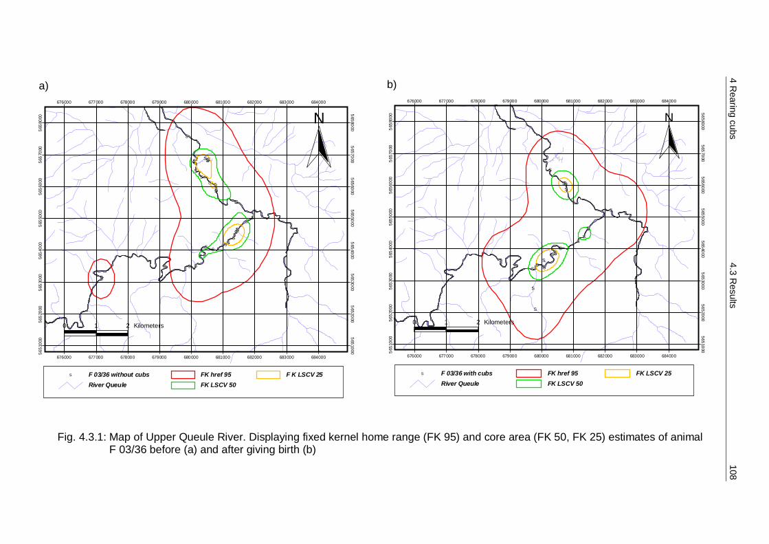
4 Rearing cubs
4.3 Results
108
#S
#S
#S
#S
#S
#S
#S
#S
#S
#S
#S
#S
#S
#S
#S
#S
#S
#S
#S
#S
#S
#S
#S
#S#S
#S
#S
#S
#S
#S
#S
#S
#S
#S#S
#S#S
0 1 2 Kilometers
N676000
676000
677000
677000
678000
678000
679000
679000
680000
680000
681000
681000
682000
682000
683000
683000
684000
684000
5651
000 5651000
5652
000 5652000
5653
000 5653000
5654
000 5654000
5655
000 5655000
5656
000 5656000
5657
000 5657000
5658
000 5658000
F 03/36 without cubs#S
River QueuleFK href 95FK LSCV 50
F K LSCV 25
#S
#S
#S
#S
#S
#S
#S
#S
#S
#S
#S
#S
#S#S
#S
#S
#S
#S
#S
#S
#S
#S
#S
#S
#S
0 1 2 Kilometers
N
F 03/36 with cubs#S
River QueuleFK href 95FK LSCV 50
FK LSCV 25
676000
676000
677000
677000
678000
678000
679000
679000
680000
680000
681000
681000
682000
682000
683000
683000
684000
684000
5651
000 5651000
5652
000 5652000
5653
000 5653000
5654
000 5654000
5655
000 5655000
5656
000 5656000
5657
000 5657000
5658
000 5658000
Fig. 4.3.1: Map of Upper Queule River. Displaying fixed kernel home range (FK 95) and core area (FK 50, FK 25) estimates of animal
F 03/36 before (a) and after giving birth (b)
a) b)

4 Rearing cubs
4.3 Results
109
Fig. 4.3.2: Map of Upper Queule River. Displaying all radio-tracking fixes of F 03/36: a) before giving birth, b) after giving birth from
August to September, and c) from October to November. Used tributaries are encircled in red
#S#S#S#S#S#S#S#S
#S#S#S#S#S#S#S#S#S#S#S#S#S#S#S#S#S#S#S#S#S#S#S#S#S#S#S#S#S#S#S#S#S#S#S#S#S#S#S#S#S#S#S#S#S#S#S#S#S#S#S#S#S#S#S#S#S#S#S#S#S#S#S#S#S#S#S#S#S#S#S#S#S#S#S#S#S#S#S#S#S#S#S#S#S#S#S#S#S#S#S#S#S#S#S#S#S#S#S#S
#S#S#S#S#S#S#S#S#S#S#S#S#S#S#S#S#S#S#S#S#S#S#S#S#S#S#S#S#S#S#S#S#S#S#S#S#S#S#S#S#S#S#S#S#S#S#S#S#S#S#S#S#S#S#S#S#S#S#S#S#S#S#S#S#S#S#S#S#S#S#S#S#S#S#S#S#S#S#S#S#S#S#S#S#S#S#S#S#S#S#S#S#S#S#S#S#S
#S#S#S#S#S#S#S#S#S#S#S
#S#S#S#S#S#S#S#S#S#S#S#S#S#S#S#S#S#S#S#S#S#S#S#S#S#S#S#S#S#S#S#S#S#S#S#S#S#S#S#S#S#S#S#S#S#S#S#S#S#S#S#S#S#S#S#S#S#S#S#S
#S#S#S#S#S#S#S#S#S#S#S#S#S#S#S#S#S#S#S#S#S#S#S#S#S#S#S#S#S#S#S#S#S#S#S#S#S#S#S#S#S#S#S#S#S#S#S
#S
#S#S#S#S
#S#S#S#S#S
#S#S#S#S#S#S#S#S#S
#S#S
#S#S#S#S#S#S#S#S#S#S#S#S#S#S#S#S#S#S#S#S #S#S#S#S#S#S#S#S#S#S#S#S#S#S
#S#S#S#S#S#S#S#S#S#S#S#S
#S#S#S#S#S#S#S#S#S#S#S#S#S#S#S#S#S#S#S#S#S#S#S#S#S#S#S#S#S#S#S#S#S#S#S#S#S#S#S
#S#S
#S#S#S#S#S #S#S#S#S#S#S
#S
#S#S#S#S#S#S#S#S#S#S#S#S#S#S#S#S#S#S#S#S#S#S#S#S
#S#S#S#S#S#S#S#S#S#S#S#S#S#S#S#S#S#S#S#S#S#S#S#S#S#S#S#S#S#S#S#S#S#S#S#S#S#S#S#S#S#S#S#S#S#S#S#S#S#S#S
#S#S #S#S#S#S#S#S#S#S#S#S#S
#S#S#S#S#S#S#S#S#S#S#S#S#S#S#S#S#S#S#S#S#S#S#S#S#S#S#S#S#S#S#S#S#S#S#S#S#S#S
#S#S#S#S#S#S#S#S#S#S#S#S#S#S#S#S#S#S#S#S#S#S#S#S#S#S#S#S#S#S#S#S#S#S#S#S#S#S#S#S#S#S#S#S#S#S#S#S#S#S#S#S#S#S#S#S#S#S#S#S#S#S#S#S#S#S#S#S#S#S#S#S#S#S#S#S#S#S#S#S#S#S#S#S#S#S#S#S#S#S#S#S#S#S#S#S#S#S#S#S#S#S#S#S#S
#S#S#S#S#S#S#S
#S#S
#S#S#S#S#S#S#S#S#S#S#S#S#S#S
#S#S#S#S#S#S#S#S#S#S
#S#S#S
#S#S#S#S#S#S#S#S#S#S#S#S#S#S#S#S#S#S#S#S#S#S#S#S#S#S#S#S#S#S#S#S
#S#S#S#S#S#S#S#S#S#S#S#S#S#S#S
#S#S#S#S#S#S#S#S#S#S#S#S#S#S#S#S#S#S#S#S#S#S#S#S#S#S#S#S#S#S#S#S#S#S#S#S#S#S#S#S#S#S#S#S#S#S#S#S#S#S#S#S#S#S#S#S#S#S#S#S#S#S#S#S#S#S#S#S#S#S#S#S#S#S#S#S#S#S#S#S#S#S#S#S#S#S#S#S#S#S#S#S#S#S#S#S#S#S#S#S#S#S#S#S#S
#S #S#S#S#S#S#S#S#S#S#S#S#S#S#S#S#S#S#S#S#S#S#S#S#S#S#S#S#S
#S#S #S
#S#S
#S#S#S#S#S
#S#S#S#S#S#S#S#S#S#S#S#S#S#S#S#S#S#S#S#S#S#S#S#S#S#S#S
#S#S#S#S#S#S#S#S#S#S#S
#S#S#S#S#S#S#S#S#S#S#S#S#S#S#S#S#S#S#S#S
#S#S#S#S#S#S#S#S#S#S#S#S#S#S#S#S#S#S#S#S#S#S#S#S#S#S#S#S#S#S#S#S#S#S#S#S#S
#S
#S#S#S
#S
#S#S#S#S#S
#S#S#S#S#S#S#S#S#S#S#S#S#S#S#S#S#S#S#S#S#S#S#S#S#S#S#S#S#S#S#S#S#S#S#S#S
#S#S#S#S#S#S#S#S#S#S#S#S#S#S#S#S#S#S#S#S#S#S#S#S#S#S#S#S#S#S#S#S#S#S#S#S#S#S#S#S#S#S#S#S#S#S#S#S#S#S#S#S#S#S#S#S#S#S#S#S#S
#S#S#S
#S#S#S#S#S#S#S#S#S#S#S#S#S#S#S#S#S#S#S#S#S#S#S#S#S#S#S#S#S#S#S#S#S#S#S#S#S#S#S#S#S#S#S#S#S#S#S#S#S#S#S#S
#S#S#S#S#S#S#S#S#S#S#S#S#S#S#S#S#S#S#S#S#S#S#S#S#S#S#S#S#S#S#S#S#S#S#S#S
#S#S#S#S#S#S#S#S#S#S#S
#S#S#S#S#S#S#S#S#S#S#S#S#S#S#S#S#S#S#S #S
#S#S
#S#S
#S#S#S#S#S#S#S#S#S#S#S#S#S
#S#S
#S#S
#S#S#S#S#S#S#S#S#S#S#S#S#S#S#S#S
#S#S#S#S#S#S#S#S#S#S#S#S#S#S#S#S#S#S#S#S#S#S#S#S#S#S#S#S#S#S#S#S#S#S#S#S#S#S#S#S#S#S#S#S#S#S#S#S#S#S#S#S#S#S#S#S
#S#S#S#S#S#S#S#S#S#S#S#S#S#S#S#S#S#S#S#S#S#S#S#S#S#S#S#S#S#S#S#S#S#S#S#S#S#S#S#S#S#S#S#S#S#S#S#S#S#S#S#S#S#S#S#S#S#S#S#S#S#S#S#S#S#S#S#S#S#S#S#S#S#S#S#S#S#S#S#S#S#S#S#S#S#S#S#S#S#S#S#S#S#S#S#S#S#S#S#S#S#S#S#S#S#S#S#S#S#S#S#S#S#S#S#S#S#S#S#S#S#S#S#S#S#S#S#S#S#S#S#S#S#S#S#S#S#S#S#S#S#S#S#S#S#S#S#S#S#S#S#S#S#S#S#S#S#S
#S#S#S#S#S#S#S
#S#S#S#S#S#S#S#S#S#S#S#S#S#S#S#S#S#S#S#S#S#S#S#S#S#S#S#S#S#S#S#S#S#S#S#S#S#S#S#S#S#S
0 0.5 1 Kilometers
N677000
677000
678000
678000
679000
679000
680000
680000
681000
681000
682000
682000
683000
683000
684000
684000
5652
000 5652000
5653
000 5653000
5654
000 5654000
5655
000 5655000
5656
000 5656000
5657
000 5657000
5658
000 5658000
F 03/36 with cubs#S
River Queule
#S
#S
#S
#S
#S
#S
#S
#S#S#S#S#S#S#S#S#S#S#S#S#S#S#S#S#S#S#S#S#S#S#S#S#S#S#S#S#S#S#S#S#S#S#S#S#S#S#S#S#S#S#S#S#S#S#S#S#S
#S#S#S#S#S#S#S#S#S#S#S#S#S#S#S#S#S#S#S#S#S#S#S#S#S#S#S
#S#S#S#S#S#S#S#S#S#S#S#S#S#S#S#S#S#S#S#S#S
#S#S#S#S#S#S#S#S#S#S#S#S#S#S#S#S#S#S#S#S#S#S#S#S#S#S#S
#S#S#S#S#S #S#S#S
#S#S#S#S#S#S#S#S#S#S#S#S#S#S
#S
#S
#S#S
#S #S#S#S#S#S#S#S
#S#S#S
#S#S#S#S#S#S#S#S#S#S#S#S#S#S#S#S#S#S#S#S#S#S#S#S#S#S#S#S#S#S#S#S#S#S#S#S#S#S#S#S#S#S#S#S#S#S#S#S#S #S
#S#S#S
#S#S #S #S
#S#S#S#S#S#S#S#S
#S#S#S#S#S#S#S#S#S#S#S#S#S#S#S#S#S#S#S#S#S#S#S#S#S#S#S#S#S#S#S#S#S#S#S#S#S#S#S#S#S#S#S#S#S#S#S#S#S#S#S#S#S#S#S#S#S#S#S#S#S#S#S#S#S#S#S#S#S#S#S#S#S#S#S#S#S#S#S#S#S#S#S#S#S#S#S#S#S#S#S#S#S#S#S#S#S
#S#S#S#S#S#S#S#S#S#S#S#S#S#S#S#S#S#S#S#S#S#S#S#S#S#S#S#S#S#S#S#S#S#S#S#S#S#S#S#S#S#S#S#S#S#S#S#S#S#S#S#S#S#S#S#S#S #S
#S#S#S#S
#S#S#S#S#S#S#S#S#S#S#S#S#S#S#S#S#S#S#S#S#S#S #S#S#S
#S#S#S#S#S#S
#S#S#S#S
#S
#S#S#S#S
#S#S
#S#S
#S#S
#S#S
#S#S
#S#S
#S
#S
#S#S#S
#S#S#S#S#S#S#S#S#S#S#S#S#S#S#S#S#S#S#S#S#S#S#S#S#S
#S#S#S#S#S#S#S
#S#S#S#S#S#S#S#S#S#S#S#S#S#S#S#S#S#S#S#S#S#S#S#S#S#S#S#S#S#S#S#S#S#S#S#S#S#S#S#S#S#S#S#S#S#S#S#S#S#S#S#S#S#S#S#S#S#S#S#S#S#S#S#S
#S
#S#S#S#S#S
#S#S#S#S#S#S#S#S#S#S#S#S#S#S#S#S#S#S#S#S#S
#S#S#S
#S#S#S#S#S#S#S#S#S#S#S#S#S#S#S
#S #S#S#S#S#S#S#S#S#S#S#S#S#S#S#S#S#S#S#S#S#S#S#S#S#S#S#S#S#S#S#S#S#S#S#S#S#S#S#S#S#S#S#S#S#S#S#S#S#S#S#S#S#S#S#S#S#S#S#S#S#S#S#S#S#S#S#S#S#S#S#S#S#S#S#S#S#S#S#S#S#S#S#S#S#S#S#S#S#S#S#S#S#S#S#S#S#S#S#S#S#S#S#S#S#S#S#S#S#S#S#S#S#S#S#S#S#S#S#S#S#S#S#S#S#S#S#S#S#S#S#S#S#S#S#S#S#S#S#S#S#S#S#S#S#S
#S
#S
#S
#S
#S
#S
#S
#S
#S
#S
#S#S
#S
#S#S
#S#S
#S#S#S #S#S #S #S
#S#S#S#S#S#S#S#S#S#S#S#S#S#S#S#S
#S#S#S
#S#S#S#S#S#S
#S#S#S
#S#S#S#S#S#S#S#S
#S#S#S
#S#S#S#S#S#S #S#S#S
#S#S
0 0.5 1 Kilometers
N677000
677000
678000
678000
679000
679000
680000
680000
681000
681000
682000
682000
683000
683000
684000
684000
5652
000 5652000
5653
000 5653000
5654
000 5654000
5655
000 5655000
5656
000 5656000
5657
000 5657000
5658
000 5658000
F 03/36 without cubs#S
River Queule
#S#S
#S#S
#S#S#S#S#S#S#S#S#S#S#S#S#S#S#S#S#S#S#S#S#S#S#S#S#S#S#S#S#S#S#S#S
#S#S#S
#S#S#S
#S#S
#S#S#S#S#S#S#S#S#S#S#S
#S
#S#S#S
#S#S#S#S#S#S#S#S#S
#S
#S#S
#S
#S
#S
#S#S
#S#S
#S#S#S
#S#S#S#S#S#S#S#S#S#S#S#S#S#S#S#S
#S#S
#S#S#S#S #S#S#S#S#S#S#S#S#S#S#S#S#S#S#S#S#S#S#S#S#S#S#S#S#S#S#S#S#S#S#S#S#S#S#S#S#S#S#S#S#S#S#S#S#S#S#S#S#S#S#S#S#S#S#S#S#S#S#S#S#S#S#S#S#S#S#S#S#S#S#S#S#S#S#S#S#S#S#S#S#S#S#S
#S#S#S#S#S#S#S#S#S#S#S#S#S
#S#S#S#S#S#S#S#S#S#S#S#S#S#S#S#S#S#S#S#S#S#S#S#S#S#S#S#S#S#S#S#S#S#S
#S#S#S#S#S#S#S#S#S#S
#S
#S#S#S#S#S#S#S#S#S#S#S#S#S#S#S#S#S#S#S#S#S#S#S#S#S#S#S#S#S#S#S#S#S#S#S#S#S#S#S#S#S#S#S#S#S#S#S#S#S#S#S#S#S#S#S#S#S#S#S#S#S#S#S#S#S#S#S#S#S#S#S#S#S#S#S#S#S#S#S#S#S#S#S#S#S#S#S#S#S#S#S#S#S#S#S#S#S
#S#S#S#S#S#S#S#S#S#S#S#S#S#S#S#S#S#S#S#S #S
#S
#S
#S#S#S#S#S#S#S#S#S#S#S#S#S#S#S#S#S#S#S#S#S#S#S#S#S#S#S#S#S#S#S#S#S#S#S#S#S#S#S#S
#S#S#S#S#S#S#S#S#S#S#S#S#S#S#S#S#S#S#S#S#S#S#S#S#S#S#S#S#S#S#S#S#S#S#S#S#S#S#S#S#S#S#S#S#S#S#S#S#S#S#S#S#S#S#S#S#S#S#S#S#S#S#S#S#S#S#S#S#S#S#S#S#S#S
#S#S#S#S#S#S#S#S#S#S#S#S#S#S#S#S#S#S#S#S#S#S#S#S#S#S#S#S#S#S#S#S#S#S#S#S#S#S#S#S#S#S#S#S#S#S#S#S#S#S#S#S#S#S#S#S#S#S#S#S#S#S#S#S#S#S#S#S#S#S#S#S#S#S#S#S#S#S#S#S#S#S #S
#S#S#S#S#S#S#S#S#S#S#S#S#S#S#S#S#S#S#S#S#S#S#S#S#S#S#S#S#S#S#S#S#S#S#S#S#S#S#S#S#S#S#S#S#S#S#S#S
0 0.5 1 Kilometers
N677000
677000
678000
678000
679000
679000
680000
680000
681000
681000
682000
682000
683000
683000
684000
684000
5652
000 5652000
5653
000 5653000
5654
000 5654000
5655
000 5655000
5656
000 5656000
5657
000 5657000
5658
000 5658000
F 03/36 with cubs#S
River Queule
a) b) c)

4 Rearing cubs 4.3 Results 110
Inactivity56%
Stationary activity
15%
Movement29%
4.3.2 Activity budget
Whilst inactive behaviour before birth has an average value of 67.5 %, it
decreases to 55.4 % for the time the female was with cubs (Fig. 4.3.3). On the
other hand, the other two behaviours, movement and stationary activity, increased.
Whilst the behaviour of stationary activity increased by 2.2 % for the time the
female was with cubs, the behaviour movement increased by 9.9 %.
Inactivity68%
Movement19%
Stationary activity
13%
Fig. 4.3.3: Percentage of displayed behaviour of female F03/36 before (A) and
after (B) giving birth
Before the southern river otter gave birth, it was not active between 03-06 hours,
little activity (4.4 %) occurred between 12-18 hours and highest activity (31.1 %)
took place between 18-21 hours (Fig. 4.3.4). Postnatally the movement pattern
changed, as movement behaviour was recorded throughout all time intervals. The
peak of movement activity was highest between 06-09 hours at 20.0 %. Lowest
value was measured between 12-15 hours (1.5 %). The movement pattern of
Lontra provocax F 03/36 is significantly different between antenatal and postnatal
periods (Chi2 = 22.04; df=7; p<0.01).
While the female southern river otter F 03/36 stayed in her den antenatally for
75.4 % of the time and was recorded for 24.6 % outside, the postnatal stay outside
of the den increased by 12.4 % to 37 % (Fig. 4.3.5).
A) B)

4 Rearing cubs 4.3 Results 111
0
5
10
15
20
25
30
35
00-03 03-06 06-09 09-12 12-15 15-18 18-21 21-24
Time
% o
f dai
ly m
ovem
ents
without cubswith cubs
Fig. 4.3.4: Ordinate dates represent averaged values in % of the total amount of
movement counts per day before and after F 03/36 gave birth. On the abscissa the 24-hour movement results are displayed in 3h intervals
0
20
40
60
80
100
antenatal postnatal
% o
f den
ning
Outside of denInside of den
Fig. 4.3.5: Percentage of time female southern river otter F03/36 spent sheltering
in den or outside of den before and after giving birth

4 Rearing cubs 4.3 Results 112
The distance the female southern river otter travelled antenatally and postnatally
differed significantly (Mann - Whitney Rank Sum Test: T=2292.00; p<0.05). The
distance the female southern river otter travelled antenatal was on average
864.8 m (SE=125.56), whereby the range was 8.68 m to 2845.9 m. Postnatally the
travelled distance was lower, on average 498.32 m (SE=46.65) with a range of
20.4 m to 372.6 m.
F 03/36
without cubs with cubs
Dis
tanc
e (m
.)
0
500
1000
1500
2000
2500
3000
*
Fig. 4.3.6: Distance travelled by animal F 03/36 between inactive phases before
and after giving birth (* p< 0.05)
Although there was difference in the time span of movements between antenatal
and postnatal period (Fig. 4.3.7), no statistical differences was found (t= - 0.154;
df=21;p=0.879).

4 Rearing cubs 4.3 Results 113
Month
April May June July Aug Sept. Oct. Nov.
Tim
e (m
in.)
0
60
120
180
240Without cubsWith cubs
mos
t lik
ely
anim
al F
03/
36 g
ave
birth
in J
uly
Fig. 4.3.7: Time span of movements per 24h of animal F 03/36 before and after giving birth
The differences of velocity in the antenatal and postnatal periods (Fig. 4.3.8) are
highly significant (Mann-Whitney Rank Sum Test: T=75993.5; p<0.001). The travel
velocity of F 03/36 was on average 1.47 km/h (SE=0.09) with a maximum speed of
10.64 km/h during the antenatal period, during the postnatal period the average
velocity was reduced (0.90 km/h; SE=0.05). However, the maximum velocity was
little higher than found antenatally at 11.21 km/h (Appendix 10.3; Tab. B).

4 Rearing cubs 4.3 Results 114
F 03/36
without cubs with cubs
Vel
ocity
(km
/h)
0
1
2
3
4 ***
Fig. 4.3.8: Calculated velocity of radio tracked southern river otter F 03/36 without
and with cubs
4.3.3 Den sites
During antenatal time the animal F 03/36 was regularly using ten dens, eight
located in the lower part (downstream) of the estimated home range (Appendix
10.3; Tab. B). During postnatal time the mother with cubs used only five dens all
located close to the tributary (average 702 m) of the natal hole.
The natal hole was located 1380 m from the Queule River in a 30m steep cliff
canyon with a bottom wide of approximately three meters. It was only possible to
locate the hole from a distance of 20 m, as the natal den itself was not accessible.
During this time (August-September) the farthest den measured from the natal den
was 3250 m away,
During October and November up to fourteen dens were used. The 14th den was
the den furthest located at 7813 m away from the natal den. Also during October
and November not all the dens which were used antenatally were visited by
mother with cubs, and five dens were used exclusively within these months.
4 Rearing cubs 4.3 Results 115
4.3.4 Additional behaviour observations
As reported for L. lutra by DURBIN (1996) the same method of “jockey style”
transportation was observed for the cubs of L. provocax, whereby the cubs bit into
the neck of the mother and were transported one by one. The second cub stayed
in place and whistled similar to a bird call with a short, clear and bright sound in a
high frequency and waited until its mother returned. The first time the cubs were
seen outside they always stayed close to the river edge and avoided the middle of
the river where the current was strongest. When passing through rapids the
mother carried her cubs, holding them by the neck, whereas the cubs show typical
carrying position. The mother always stayed close to her cubs, caching
crustaceans, and returning to the cubs to feed them. The cubs were observed to
whistle when their mother arrived and would take the crustacean out of her mouth.
KRUUK & MOORHOUSE (1990), WATT (1991) (cited in: DURBIN, 1996) assume
that cubs learn hunting by imitating the foraging behaviour of their mother.
On three occasions cubs followed F03/36 out of the water to mark on the river
bank. Cubs never were seen marking. However, in November for the first time two
smaller fresh spraints were found at one of F 03/36 marking sites. In November
(probably four months after the birth) one cub was observed swimming
independently alongside the mother, although on some occasions the cub still
used the “jockey style” even when the cub had almost reached the body length of
the mother. At the end of this study, only one cub was observed with its mother.

4 Rearing cubs 4.4 Discussion 116
4.4 Discussion
4.4.1 Home range
As predicted, whilst rearing the cubs the female F 03/36 used tributaries, which
were not visited antenatal or in previous years and which were less anthropogenic
disturbed as no roads, or houses were nearby. Buildings or roads were more than
1300 m away. This is contrary to the findings for the European otter, where even
natal holes were close to roads or villages (DURBIN, 1996; RUIZ-OLMO et al.,
2005). Consequently, by using tributaries, the postnatal core area shifted
upstream for the time F 03/36 was moving with cubs. This behaviour of using
different patches when travelling with cubs was also reported for L. lutra by several
authors (e.g. DURBIN, 1996; KRUUK, 1995; RUIZ-OLMO et al., 2005). It has been
suggested that the use of different patches is a strategy to minimizes intraspecific
disturbance in bordering ranges, which has also been shown for other carnivores
such as brown bears Ursus arctos (DAHLE & SWENSON, 2003) as they attempt
to avoid conflicts. Nevertheless, the studied female might have been also
restricted in their movements to her cubs’ capabilities, as they were not able to
swim with the same velocity as the mother (Appendix 10.3; Tab. A). However, as
the cubs aged and body size was almost similar to the mothers body size, river
sections and tributaries which were further away and used by the mother before
were visited regularly and the former, more ‘protective’, tributaries were not visited
again.
4.4.2 Activity budget
The increase in activity and movements of F 03/36 with cubs, as well as the
increase in time outside dens during the postnatal period is assumed to be a
logical consequence of the higher demand for nutrition as is known for other
species (e.g. GARSHELIS & PELTON, 1980).
However, as a consequence of travelling with cubs the otter’s activity decreased,
especially movement periods, travelled distances and velocity. Furthermore, when
travelling for longer distances, cubs were transported by the mother in jockey style
one by one. These findings are consistent with observations on L. lutra by
SAAVEDRA BENDITO (2002) and DURBIN (1996). Short travel distances and

4 Rearing cubs 4.4 Discussion 117
staying close to den sites may be a strategy to avoid conflicts and increase
security (DAHLE & SWENSON, 2003; DURBIN, 1996; ZALEWSKI, 1997).
It is unknown if an internal or external factor influences the low activity period
between 12-18 hours of the studied animal. However, human avoidance cannot
explain the low activity period as forest workers and farmers were active during the
whole day.
4.4.3 Den sites
As mentioned by JENKINS (1980) and DURBIN (1996) the selection of a natal
hole in a tributary could be to provide safety against flooding. This was the case in
the study area as flooding occurs in autumn, winter and spring (time of parturition).
The other dens which were used by the female southern river otter antenatally
were located 40 - 300 cm above the water level (measured in summer) and not
secure against flooding. Furthermore, the natal hole was undisturbed by any kind
of anthropogenic disturbance.
The number of dens used in the first period of postnatal time (August –
September) was low compared to antenatal time and reached a maximum in the
second period (October – November) as the cubs were getting older and travelled
further distances. During the time the mother was travelling with cubs some dens
were used exclusively. The findings of dens used exclusively with cubs is
consistent with observations by DURBIN (1996) for the European otter in
Scotland. These exclusively used dens may be unknown to other individual otters
and serve to avoid intraspecific conflicts, or may have been used because they
were larger and offered more space for the family group.

4 Rearing cubs 4.4 Discussion 118
4.4.4 Reproductive cycle and parental care – a model
Throughout the five year study and particularly in the present study, where mother
and cubs were radio tracked, different observations such as menses, copulation,
travelling with cubs and approximate birth time were noted and a model of the
reproductive cycle was created (Fig. 4.3.9; Appendix 10.3; Tab. C).
All otter species show a continual polyoestrus, except the northern river otter
Lontra canadensis (ESTES, 1989).
However, the Eurasian otter shows both continual polyoestrus and seasonal
polyoestrus. This has been reported by KRUUK (1996) who demonstrated a
seasonal polyoestrus for L. lutra in Shetland, but a flexible timing of reproduction in
other areas (KRUUK, 1995).
For the southern river otter seasonal breeding is assumed, as cubs were never
seen all year round. Observations of female with cubs, also termed family groups,
were recorded in October 1999 (two cubs), February 2001 (one cub), November
2001 (two cubs), October 2002 (two cubs), September 2003 (two cubs) and in
November 2003 (one cub). Also in the south of Chile cubs were observed in
September and October (PARERA, 1996). A polyoestrus is also assumed in the
southern river otter, as the female animal showed menses during captivity and
gave birth later.
The time of conception was estimated by menses, which occurred in January 2001
and April 2002 and observed copulations in December 2001. These results are
similar to the Eurasian otter L. lutra (KRUUK, 1995; RUIZ-OLMO et al., 2005;
SANDELL, 1989), where mating mainly occurred in the same season but different
months as L. lutra inhabits the northern hemisphere and the southern river otter
the southern hemisphere.
The date for parturition was calculated as July when the female F 03/36
disappeared from her usual home range and was discovered in a tributary, where
she stayed for two months. She was then seen in September with cubs. The
assumed two month stay in the natal hole is consistent with L. lutra
(HEGGBERGET & CHRISTENSEN, 1996; KRUUK et al., 1987; KRUUK, 1995;
RUIZ-OLMO et al., 2002), and with observations by PARERA (1996).
An average gestation period of 63 days, as is known for other otter species (for
review see CHANIN, 1985) is not assumed for L. provocax as copulation also
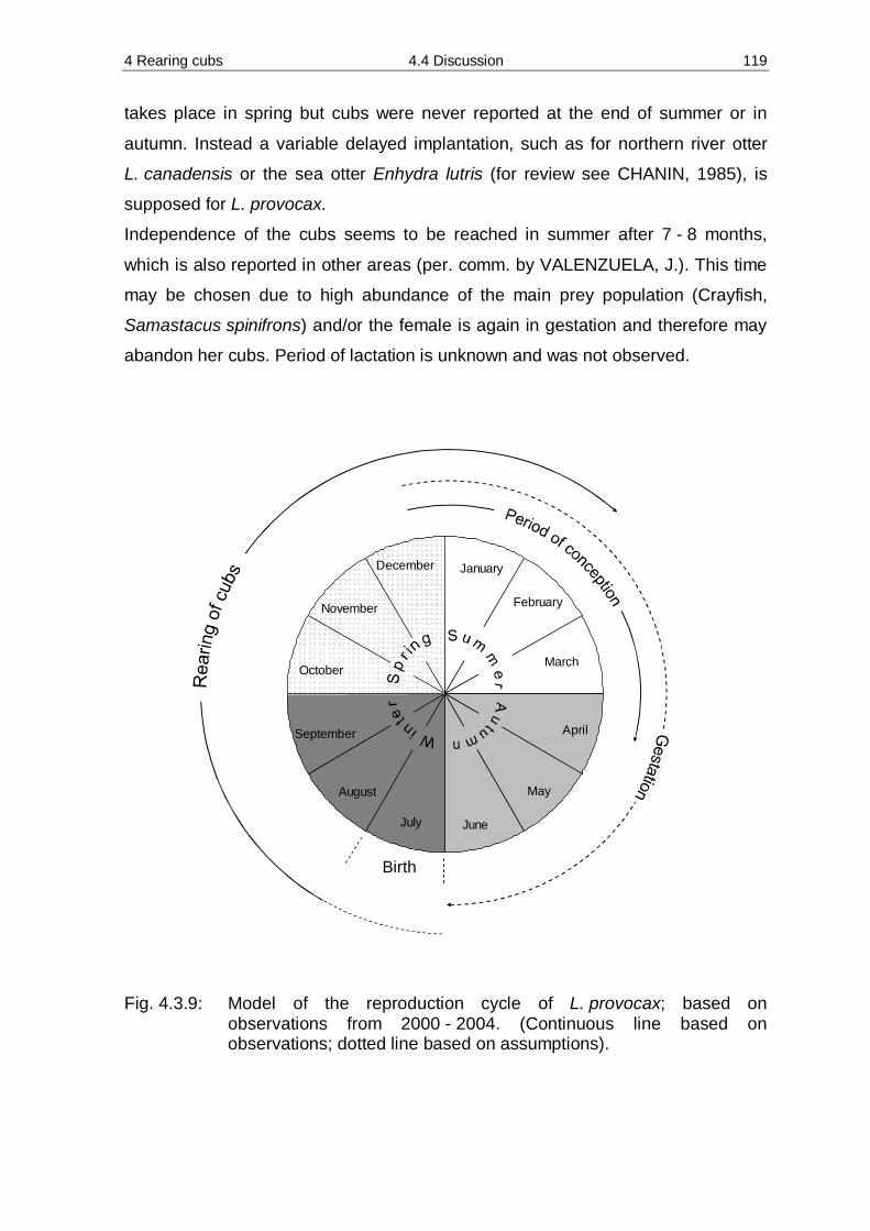
4 Rearing cubs 4.4 Discussion 119
takes place in spring but cubs were never reported at the end of summer or in
autumn. Instead a variable delayed implantation, such as for northern river otter
L. canadensis or the sea otter Enhydra lutris (for review see CHANIN, 1985), is
supposed for L. provocax.
Independence of the cubs seems to be reached in summer after 7 - 8 months,
which is also reported in other areas (per. comm. by VALENZUELA, J.). This time
may be chosen due to high abundance of the main prey population (Crayfish,
Samastacus spinifrons) and/or the female is again in gestation and therefore may
abandon her cubs. Period of lactation is unknown and was not observed.
March
February
JanuaryDecember
November
October
September
August
July June
May
April
Birth
Fig. 4.3.9: Model of the reproduction cycle of L. provocax; based on observations from 2000 - 2004. (Continuous line based on observations; dotted line based on assumptions).

5 Prey availability 5.1 Introduction 120
5 Prey availability, diet composition and food competition
5.1 Introduction
5.1.1 Prey availability
To understand what determines the distribution and abundance of organisms is an
essential goal in ecology. One of these factors is food or prey availability as it has
a powerful influence on animal populations in both the determination of habitable
areas and the number of individuals which these areas can support (KREBS,
1994). Food availability is a concept which was first introduced by NEIL (1938)
who was analysing the food of brown trout Salmon salar, in relation to its
accessibility. If enough food is available the number of individuals an area can
support increases. On the other hand, if prey availability is limited, animals which
depend on prey will face higher intraspecific competition and have to expand their
home range or disperse. Thus show SOMERS & NEL (2004) that the home-range
length of the Cape clawless otters Aonyx capensis, was correlated with high food
density patches. Also, differences in prey diversity between habitats influence the
dietary breadth of a species (PIELOU, 1975). Factors such as these can have far-
reaching effects on the demographic stability of populations (RICKLEFFS, 1973).
In the time of reproduction adults must adjust their own energy requirements with
those of their offspring (STEARNS, 1992), thus has prey availability a strong effect
on reproductive success like pup mortality and timing of birth is described by
several authors for sea lions Otavia flavescens, (SOTO et al., 2004); wolverine
Gulo gulo (PERSSON, 2005), kit foxes Vulpes velox (WHITE & RALLS, 1993) and
European otter Lutra lutra (HEGGBERGET & CHRISTENSEN, 1996; RUIZ-OLMO
et al., 2002).
Prey availability is influenced by numerous factors, such as habitat structures,
temperature, activity, and competition; and, prey availability is also sensitive to
environmental changes (e.g. KEDZIERSKI & SMOCK, 2001). The most important
determinants of the composition and structure of prey communities, however, are
abiotic environmental factors (SMITH & SMITH, 2000). Therefore, the physical and
chemical factors of water are very important for aquatic species. Though generally
less visible than biotic factors, these factors also significantly affect the
abundance, distribution and diversity of species (REASH & PIGG, 1990) and in
5 Prey availability 5.1 Introduction 121
this case of the prey species. Therefore, physico-chemical factors of water can
have an indirect and far-ranging effect on the distribution of the southern river
otter.
5.1.2 Food competition
Competition between two species exists when they use the same limited resource
or harm one another while exploiting a resource (KREBS, 1994). To avoid
competition coexisting species should possess niche differentiation or resource
partitioning (BEGON et al., 1996). If a strong competition exists, and the species
are not able to differentiate into niches, one species may be displaced; or in other
words, one species may become extinct as it reaches a suboptimal state (KREBS,
1994).
The most important niche dimensions for coexisting vertebrates are food, habitat
use and activity patterns (SCHOENER, 1986). Several authors show that this is
also the case for coexisting mustelides (BONESI et al., 2004; MEDINA, 1997;
PERRIN & CARUGATI, 2000; SOMERS & PURVES, 1996; WU, 1999).
One of the main factors which may negatively influence an individual from
maximising its energy intake, and thereby forcing it to shift its diet, is interspecific
food competition (BONESI et al., 2004). For carnivore predators, food is an
especially essential resource, and its partitioning among sympatric species is
crucial for coexisting (JEDREZEJEWSKI et al., 1989).
One theory, based on the evolutionary history of communities, proposes that
competition resulted in adaptations that serve to minimize competitive effects
(KREBS, 1994). As long as the community and environmental parameters are
stable, or change slowly, strong competition may not exist. However, if alien
species are introduced, the competition may increase and lead to extinction of
native species (e.g. LOCKWOOD et al., 2007; MAGIN et al., 1994).
As in Eurasia (JEDRZEJEWSKA et al., 2001), the non-native American mink
Mustela vison established free-living populations from farm escapees in Chile
(MEDINA, 1997) and competitive interferences between American mink and otter
are suggested by several authors (e.g. CHANIN, 1981; CLODE & MACDONALD,
1995; ERLINGE, 1972). MEDINA (1997) found little competition for space and
food between American mink and southern river. However, interactions between
both species depend on each respective situation.

5 Prey availability 5.1 Introduction 122
5.1.3 Diet composition
The diet composition for each specific animal is a consequence of external factors
such as predation risk, prey availability and social interactions, as well as internal
factors such as the animal’s condition, age, sex and reproductive state. In addition,
morphological aspects such as its skull and mouth shape, as well as dentition,
play an important role in prey selection (CARSS, 1995; LITVAITIS, 2000).
Mustelides are primarily carnivorous; they will, however, consume vegetation. The
consumption of vegetation depends on the species and on the season of the year.
In this case they are known as opportunistic feeders, rather than specialists.
Mustelides tend to hunt in terrestrial, arboreal and aquatic habitats; and, some
species prey on animals larger than themselves (VAUGHAN et al., 2000).
Otters are well-adapted to hunt aquatic prey and are commonly known as
opportunistic food generalist (CHANIN, 1985). However, the diet composition of
otter depends also on species, habitat and prey type availability (CARSS, 1995;
CHANIN, 1985). Thus, according to JEDRZEJEWSKA (2001), the diet of L. lutra
changes with relation to specific habitats. Fish are seen as the dominant food
when otters are close to the seashore; but crustaceans and amphibians become
more important food sources in areas closer to inland waters.
The otter species Lutra lutra, Lutra maculicollis, Lontra canadensis,
Lontra longicaudis as well as Pteronura brasiliensis are commonly classified as
piscivouros, because fish consumption generally dominates their diet (BONESI et
al., 2004; DOLLOF, 1993; PERRIN & CARUGATI, 2000; REID et al., 1994;
ROSAS et al., 1999). Enhydra lutris feeds mainly on invertebrates (CHANIN,
1985), whereas the diet of Aonyx capensis is dominated by crabs (SOMERS &
PURVES, 1996). Food such as crayfish, frogs, mammals and birds are usually
seasonal components of their diet, and are generally regarded as a secondary
food source. In order to establish protocol for the conservation of otters,
observations on diet are useful to determine how the species deals with changes
in aquatic systems in terms of both prey population and habitat availability
(ANOOP & HUSSAIN, 2005).
Most research on diet composition has been conducted and published on common
otter species, such as L. lutra, L. canadensis and E. lutris, but is scarce for
secretive and difficult-to-observe species like the southern river otter.

5 Prey availability 5.1 Introduction 123
Previous statements for the diet composition of Lontra provocax were made as a
result of faeces analysis which showed that crustacean species (Samastacus
spec., Aegla spec.) comprise the vast majority of collected faecal sample remains
in freshwater habitats (CHEHÉBAR & PORRO, 1998; MEDINA, 1997; MEDINA,
1998; MEDINA-VOGEL et al., 2004). However food availability was not
considered.
5.1.4 Aims
The principle aim of this chapter is to determine whether the southern river otter is
a food specialist or is compelled to nourish on the only available prey items.
More specific objectives are to: 1) determine the seasonal variation of prey
species in faecal samples collected over a 12 month period; 2) determine the
factors which are crucial for prey availability; 3) calculate required quantity of main
prey for basic metabolic requirements; 4) compare the diet composition and the
degree of food similarity between American mink and southern river otter.

5 Prey availability 5.2 Methods 124
5.2 Methods
Estimation and comparison of prey availability and diversity was conducted in the
Upper Queule River (UQR). To estimate prey availability, amphibian sampling and
electrofishing was carried out. Nine patches were examined for occurrence of
amphibians. Electrofishing was employed at ten stations in the UQR and on one
additional station in the nearby Mahuidanche River during two consecutive dry
seasons (adapted from RUIZ-OLMO, 1998, CARSS et al., 1998). Spraints, for diet
analysis were collected along the UQR. Water samples for detailed
physico-chemical analysis were collected monthly on five stations in UQR and two
stations in Mahuidanche River. Figure 5.2.1 is displaying the stations for
electrofishing, amphibian inventory and water sample stations.
0 5 10 KilometersN
660000
660000
665000
665000
670000
670000
675000
675000
680000
680000
685000
685000
5650
000 5650000
5655
000 5655000
5660
000 5660000
5665
000 5665000
5670
000 5670000
Fig. 5.2.1: Stations where water samples were taken, electrofishing and amphibian sampling took place; QWS = water sampling stations at Queule River, MWS = water sampling station at Mahuidanche River, EF = electrofishing stations; A = amphibian sampling patches; only main streams are displayed; map is displayed in UTM coordinates
Mahuidanche River
Queule River
QWS 01
QWS 02
MWS 01 + 02
QWS 03
EF 01 – 09 (Q 01 – 09)
EF 11 (M 01)
EF 10 (Q 10)
AS 01 - A 07
AS 08
QWS 04 Villa Boldo
Tolten
QWS 05
AS 09

5 Prey availability 5.2 Methods 125
Contents of the stomach of dead southern river otter finds were defined, since they
provide insight into the nutritional components (preyed species) which are
normally absorbed in the digestive tract and can not be detected in faeces
samples.
5.2.1 Sampling methods
5.2.1.1 Amphibians
Inventories of amphibians were carried out using two methods: patch sampling
and strait-line drift fences with pitfall traps.
Patch sampling is a method which can be used to examine the densities of
amphibians in an environment which are often associated with specific
microhabitats or patches, e.g. logs, trees buttresses, bromeliads (JAEGER et al.,
1982). Patch sampling can be used to determine the number, relative
abundances, and densities of species present in discrete subunits of an area of
interest. Given that patches are sampled at random in an area and that each patch
constitutes an independent sample, it is possible to make statistical inferences of
data with sufficiently large sample size. These inferences can be used either for
monitoring or inventory. The number of patches required for statistical treatments
depend on the variance in the data, which is not known a priori.
Drift fences with pitfall traps are used to inventory and monitor populations of
amphibians and reptiles (SZARO et al., 1988). Drift fences intercept amphibians
moving on the surface of the ground within a several meter area and redirect them
into a pitfall. Pitfall traps without fences act in a similar manner, but individual traps
intercept only a few square centimetres of ground (CORN & BURY, 1990).
All captured amphibians were sexed; weighed in grams on a digital scale (DIPSE
XL500; 500 g/0.1 g) and measured for length with a calliper from snout to vent
in mm. Nine sites for investigation were chosen at random. The microhabitat was
characterised by following variables: sand/stones, silt, leaf litter, marsh grass
Juncetum procerii, grass (< 10 cm), herbs (> 10 cm), logs, roots, bushes, trees
(< 10 m) and big trees (> 10 m).

5 Prey availability 5.2 Methods 126
5.2.1.2 Fish and crustaceans
Two primary methods exist for catching crustaceans: crustacean traps and “red de
palito”. Crustacean traps generally only help to determine the occurrence species,
not total counts. “Red de palito” is a simple method in which a researcher holds a
setup of two sticks connected by a 5 mm wide, conically shaped net, such that the
sticks are perpendicular to the ground. The opening of the net has a height of 1 m
with its lower portion lined with a metal chain to maintain contact with the riverbed.
The researcher collects samples by walking backwards in the river against the
current while flipping up objects on the riverbed with his feet. The river current
sends the animals hidden under the substrate into the net (5.2.2).
Fig. 5.2.2: Function of “red de palito”
Total length of crustaceans was measured in mm with a calliper (rostrum to final
pleon) and weighed in grams on a digital scale (DIPSE XL500; 500 g/0.1 g). The
rostrum of each crustacean was measured separately. This was done to
determine if a correlation of rostrum length to crustacean weight exists, which
provides a basis for discover prey weight or rather prey size preferences in
crustacean selection out of faeces samples.
For electrofishing stop-nets were used to reduce emigration and leeway of
stunned fish during fishing operations. By following a standard procedure, the river
section was fished at least three times upstream in an s-shape manner, with a
30 minutes interval between removals (BOHLIN et al., 1989; CAMPOS &
MORENO, 1985; PERRIN & CARUGATI, 2000) until no new samples were
collected. Stunned fish were transferred into buckets, measured with a calliper
(fork-length in mm) and identified as species. Each fish was weighed in grams
(DIPSE XL500; 500 g/0.1 g) and scales were removed with forceps and stored as
reference material.
walking direction
“red de palito” – sticks with net
water level
river current

5 Prey availability 5.2 Methods 127
In both cases, “red de palito” and electrofishing, a river section of 100 m2 was
investigated and all riverbed structures were noted. The riverbed structure was
classified into sand (≤ 2 mm), gravel (> 2 - ≤ 63 mm), stones
(> 63 mm - ≤ 500 mm), rocks (> 500 mm), woody debris (dead wood like logs and
branches in river), trees/roots and aquatic plants. The classification of grain size
was abutted on DIN 4022, except rocks. Additionally, the type of riverbed structure
where each single species was captured was listed. After the collection and
determination procedure all animals were released in the river section from which
they were taken out.
5.2.2 Spraint analysis
Otter spraints were collected during each survey; each day for 14 days of a month
for diet analysis. Additionally, mink scats which were placed on the same sites of
otter spraints were collected and determined. After storing and labelling the faeces
samples in plastic bags, they were washed and rinsed with washing agent in the
laboratory. The spraints then were placed in a drying cupboard at a temperature of
75 °C for 72 hours and stored in labelled paper bags for later analyses.
With the help of a stereoscopic microscope (3x – 12x) and a magnifying glass (8x),
prey remains found in dried spraints were identified and compared with reference
materials obtained in the same or nearby river sections. According to
KLOSKOWSKI (1999; 2000) maxillaes, articularies and dentaries of fish remains
from collected faeces samples were used to identify fish species. Intact rostrums
of crustacean were measured with a calliper in mm for later correlation analysis of
crustacean body length and weight. The diet composition of Lontra provocax was
specified according the definition by CARSS & PARKINSON (1996) as frequency
of occurrence, whereby the results are presented as percentage frequency – the
total number of spraints in which a certain prey artefact was found, and as relative
frequency – the frequency an artefact was found, presented as percentage of all
items registered. It was attempted to verify all prey artefacts to species level.
However, some fish remains were unidentifiable and therefore combined into one
class. The same was done with rodent and bird in mink samples.

5 Prey availability 5.2 Methods 128
5.2.3 Water analysis
Water samples were taking monthly from April 2003 to March 2004, excluding May
2003 due to otter trapping activity. Samples were taken at five stations on the
Queule River (QWS 01 - QWS 05) and at two stations at the Mahuidanche River
(MWS 01 - MWS 02). Water samples were obtained with a Friedinger-water-sampler
from 0.50 m depth, but dependent on the season e.g. summer, the sample depth
averaged 0.30 m. Two samples were taken from each station, one with a
membrane filter (SCHLEICHER & SCHWELL, GERMANY; pore size 0.2 µm) and
one left unfiltered. Samples were stored in 1litre plastic bottles (PE). Additionally,
river current was measured with the drift body (surface float) method
(SCHWOERBEL, 1994), and river width and depth were noted.
Water sample station 1 (QWS 01) was influenced by forest management and
situated between pine plantations close to a gravel road. Clear-cutting occurred
several times during sampling years. The riverbed structure consisted of gravels.
River station 2 (QWS 02) is located close to a school and pasture land which was
seldom used. The riverbed structure consists of sand. The third station (QWS 03)
was situated in the ombrophilous swamp forest with sand, roots and woody debris
as riverbed structure. Station 4 (QWS 04) was directly behind the village Villa
Boldo, with sand and algae on the riverbed. Station 5 (QWS 05) lay behind the
village Tolten with identical riverbed structure as in QWS 04. While the waste water
from Villa Boldo drained into the River Queule, the village Tolten lead its waste
water into the nearby river Tolten. Two additional stations MWS 01 and MWS 02
located in the river Mahuidanche were sampled too. Station MWS 01 was on a
normal river section whereas station MWS 02 lay on a tributary stream with no
current in summer and adjoined heavily used grazing land. Water sample stations
QWS 01, QWS 02, QWS 03 and MWS 02 also were sections where electrofishing was
carried out.
Physical measurements
Water temperatures were obtained using the mounted standard thermometer in
the Friedinger-water-sampler, with an accuracy of temperature readings of 0.2 °C.
Water turbidity was measured by spectrophotometry (Model 2260, DELTA
SCIENTIFIC, Inc.), at 440 nm. Conductivity and pH - values were acquired with a
pH meter and conductivity meter (HANNA Instruments, U.S.A.).
5 Prey availability 5.2 Methods 129
Chemical measurements
For the measurement of water quality, the chemical parameters, listed in
Table 5.2.1 were analysed. This study followed the standard methods (APHA,
1980; ZAHRADNIK, 1981) for analyses of relevant parameters. Titration was used
to measure alkalinity, chloride, dissolved oxygen, and German hardness. The
parameter ammonia, chemical oxygen demand (COD), nitrate, nitrite, nitrogen,
phosphor, silicate and sulphate were measured using a double-beam
spectrophotometer (UV-150-02, SHIMADZU Corporation, Japan) (for specific
wave length see Tab. 5.2.1).
Conductivity, pH, and alkalinity, were measured immediately on the premises.
Water samples for dissolved oxygen were preserved by acidification. The analysis
of additional parameter were carried out (phosphorus, ammonia, nitrate, nitrite,
silicate, sulphate, chloride, total hardness) after a briefly freezing water samples in
the limnology laboratory of the zoology department at the University Austral, Chile
(Laboratorio Limnológico del Instituto de Zoología, Universidad Austral de Chile).
Filtered water samples were used for analyses of silicate and nitrite content.
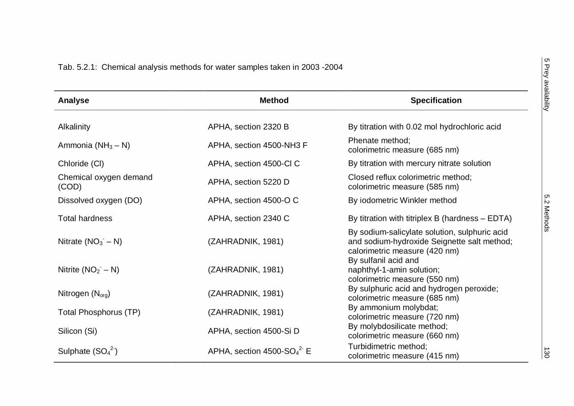
5 Prey availability
5.2 Methods
130
Tab. 5.2.1: Chemical analysis methods for water samples taken in 2003 -2004
Analyse Method Specification
Alkalinity APHA, section 2320 B By titration with 0.02 mol hydrochloric acid
Ammonia (NH3 – N) APHA, section 4500-NH3 F Phenate method; colorimetric measure (685 nm)
Chloride (Cl) APHA, section 4500-Cl C By titration with mercury nitrate solution
Chemical oxygen demand (COD)
APHA, section 5220 D Closed reflux colorimetric method; colorimetric measure (585 nm)
Dissolved oxygen (DO) APHA, section 4500-O C By iodometric Winkler method
Total hardness APHA, section 2340 C By titration with titriplex B (hardness – EDTA)
Nitrate (NO3- – N) (ZAHRADNIK, 1981)
By sodium-salicylate solution, sulphuric acid and sodium-hydroxide Seignette salt method; calorimetric measure (420 nm)
Nitrite (NO2- – N) (ZAHRADNIK, 1981)
By sulfanil acid and naphthyl-1-amin solution; colorimetric measure (550 nm)
Nitrogen (Norg) (ZAHRADNIK, 1981) By sulphuric acid and hydrogen peroxide; colorimetric measure (685 nm)
Total Phosphorus (TP) (ZAHRADNIK, 1981) By ammonium molybdat; colorimetric measure (720 nm)
Silicon (Si) APHA, section 4500-Si D By molybdosilicate method; colorimetric measure (660 nm)
Sulphate (SO42-) APHA, section 4500-SO4
2- E Turbidimetric method; colorimetric measure (415 nm)
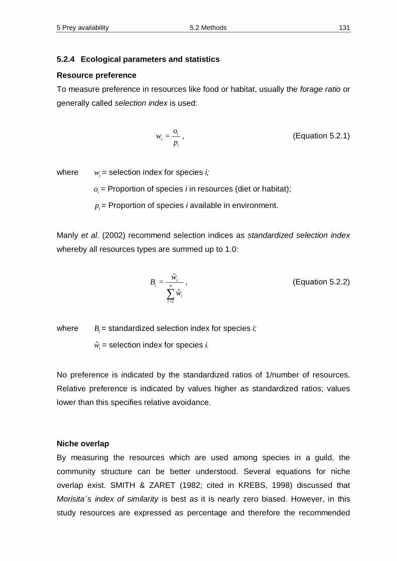
5 Prey availability 5.2 Methods 131
5.2.4 Ecological parameters and statistics
Resource preference
To measure preference in resources like food or habitat, usually the forage ratio or
generally called selection index is used:
i
ii p
ow = , (Equation 5.2.1)
where iw = selection index for species i;
io = Proportion of species i in resources (diet or habitat);
ip = Proportion of species i available in environment.
Manly et al. (2002) recommend selection indices as standardized selection index
whereby all resources types are summed up to 1.0:
∑=
= n
ii
ii
w
wB
1
ˆ
ˆ, (Equation 5.2.2)
where iB = standardized selection index for species i;
iw = selection index for species i.
No preference is indicated by the standardized ratios of 1/number of resources.
Relative preference is indicated by values higher as standardized ratios; values
lower than this specifies relative avoidance.
Niche overlap
By measuring the resources which are used among species in a guild, the
community structure can be better understood. Several equations for niche
overlap exist. SMITH & ZARET (1982; cited in KREBS, 1998) discussed that
Morisita´s index of similarity is best as it is nearly zero biased. However, in this
study resources are expressed as percentage and therefore the recommended

5 Prey availability 5.2 Methods 132
measure of niche overlap is Horn’s Index (RICKLEFS & LAU, 1980; SMITH &
ZARET, 1982; cited in KREBS, 1998).
2log2loglog)log()(∑ ∑ ∑−−++
= ikikijijikijikijO
ppppppppR , (Equation 5.2.3)
where OR = Horn’s index of overlap for species j and k;
ijp = Proportion resource i is of the total resources utilized by species j;
ikp = Proportion resource i is of the total resources utilized by species k.
Niche breadth
The niche breadth (niche size, niche width) indicates the specialisation of a
species. It can be quantitatively measured by observing the distribution of
individuals within resources (KREBS, 1998). In this study the Levins’s
standardized niche breadth was used, which can be expressed on a scale from 0
to 1.0.
∑= 2
2
jNYB , (Equation 5.2.4)
11
−−
=nBBA , (Equation 5.2.5)
where B = Levins’s measure of niche breadth;
jN = Number of individuals found in or using resource state j;
∑= jNY = Total number of individuals sampled;
AB = Levins’s standardized niche breadth;
n = Number of possible resource states.
As is often found in the literature, the number of frequently used resources is
mentioned. This information will be used as well as Levins’s standardized niche
breadth in the current study.

5 Prey availability 5.2 Methods 133
Species diversity
Diversity is an independent parameter of the species community. It is calculated
via species number and dominance structure. In general, two categories of
diversity index exist, Type I indices and Type II indices. Whereby the Type I
indices are sensitive to rare species, Type II indices are most sensitive to changes
in common species. The most popular diversity index is the Shannon – Wiener
index (sometimes wrongly cited as Shannon – Weaver index (WASHINGTON,
1984) ). However, the Shannon – Wiener index describes more the rare species in
the community analysis (Type I), whereby the Simpson’s index weight the
common species more (Type II) (KREBS, 1998). Shannon – Wiener and
Simpson’s index are measuring exclusively the proportion of individual species to
each other, consequently reference values like sample volume or sample area
remain without influence. The higher the number of species and/or balanced the
occurrence of species, the higher the diversity is in the community.
In this study the Simpson’s index is used for measuring species diversity, but to
allow for comparison with data presented in the literature, the Shannon – Wiener
index calculated with ln (natural logarithm) is also listed in the results. The
Simpson’s index can be calculated by the equation:
∑−=− 2)(11 ipD , (Equation 5.2.6)
where ( )D−1 = Simpson’s index of diversity;
ip = Proportion of individuals of species i in the community.
The used equation for the Shannon – Wiener index is:
∑=
−=s
iiiS ppH
1ln* , (Equation 5.2.7)
where SH = Shannon – Wiener index of species diversity;
s = Number of species;
ln = natural logarithm;
ip = Proportion of total sample belonging to i-th species.

5 Prey availability 5.2 Methods 134
Evenness Evenness or equitability is a measure that quantifies how equally species are
represented in a community, whereby the unequally represented community is
quantified against a hypothetical equal distribution. When the abundances of all
species in a community are equal, evenness is maximal. KREBS (1998) discuss
that the Smith and Wilson index is the best available evenness index as it is
independent of species richness and is sensitive to both rare and common species
in the community. The index is defined as:
−
=
∑ ∑= =
s
i
s
jjeie ssnn
E
1
2
1
var
)/)(log)(logarctan
2
π
, (Equation 5.2.8)
where varE = Smith and Wilson’s index of evenness;
in = Number of individuals in species i in sample;
jn = Number of individuals in species j in sample;
s = Number of species in entire sample.
Species similarity index
To discern how separate areas vary in their fauna composition, a similarity
coefficient can be used to measure this difference. Of the many measures of
similarity found in the literature, this study uses two, the Soerensen’s similarity
coefficient and the Renkonen index.
The Soerensen’s similarity coefficient allows for a simple comparison of species
communities. It takes into consideration both the number and type of species
common to two comparable habitats.

5 Prey availability 5.2 Methods 135
The Soerensen’s similarity coefficient is:
cbaS s ++
=2
2 , (Equation 5.2.9)
where SS = Soerensen’s similarity coefficient;
a = Number of species in sample A and sample B;
b = Number of species in sample B but not in sample A;
c = Number of species in sample A but not in sample B.
The Sorensen’s similarity coefficient produces values between 0 % to 100 %; the
higher the value the higher the similarity of species composition (MÜHLENBERG,
1993).
The compliances of dominance proportion between two species communities can
be calculated with the Renkonen index. To measure the similarity with the
Renkonen index, all community samples have to be standardized to percentages
(KREBS, 1998). The equation is:
∑=i
iie ppR ),( minimum 21 , (Equation 5.2.10)
where eR = Renkonen index, similarity between sample 1 and sample 2;
ip1 = Percentage of species i in community sample 1;
ip2 = Percentage of species i in community sample 2.
WOLDA (1981; cited in KREBS, 1998) describes this similarity measure as the
best quantitative similarity coefficients available. The index ranges from 0 % (no
similarity) to 100 % (complete similarity).
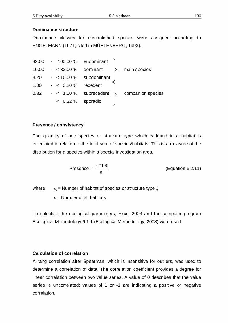
5 Prey availability 5.2 Methods 136
Dominance structure
Dominance classes for electrofished species were assigned according to
ENGELMANN (1971; cited in MÜHLENBERG, 1993).
32.00 - 100.00 % eudominant
10.00 - < 32.00 % dominant main species
3.20 - < 10.00 % subdominant
1.00 - < 3.20 % recedent
0.32 - < 1.00 % subrecedent companion species
< 0.32 % sporadic
Presence / consistency
The quantity of one species or structure type which is found in a habitat is
calculated in relation to the total sum of species/habitats. This is a measure of the
distribution for a species within a special investigation area.
nni 100*
=Presence , (Equation 5.2.11)
where in = Number of habitat of species or structure type i;
n = Number of all habitats.
To calculate the ecological parameters, Excel 2003 and the computer program
Ecological Methodology 6.1.1 (Ecological Methodology, 2003) were used.
Calculation of correlation
A rang correlation after Spearman, which is insensitive for outliers, was used to
determine a correlation of data. The correlation coefficient provides a degree for
linear correlation between two value series. A value of 0 describes that the value
series is uncorrelated; values of 1 or -1 are indicating a positive or negative
correlation.

5 Prey availability 5.2 Methods 137
Cluster analysis
The cluster analysis was used to classify the electrofished sections by species
abundance and amphibian microhabitats. Cluster analysis is used to build
classifications of a series of samples. In this study average linkage clustering is
used because it is capable of determining the dissimilarity between cluster
average values. The most recommended and most frequently used clustering
strategy is the unweighted pair-group method using arithmetic averages
(UPGMA)(KREBS, 1998). In the UPGMA the distance between two clusters is
computed as the average distance between all pairs of objects in the two different
clusters. The Euclidean distance setting was used for amphibian microhabitats
and the dissimilarity coefficient for river species communities.
Statistical tests
Verification of normal distribution was carried out using the Kolmogorov-Smirnov
test. Because samples were not drawn from a normal distribution, differences in
weight and length between two amphibian species were analysed for significance
using the Mann-Whitney rank sum test. Using 2χ - Test, the following frequencies
were tested: between investigation sites of amphibian samplings; riverbed
structure composition of electrofished areas; abundance and biomass of two
consecutive years; mink and southern river otter spraints; and between crustacean
and fish biomass. ANOVA was applied for the analysis of variances by the
examination of species occurrences in riverbed structure by electrofishing and by
average weight of captured species by electrofishing. If samples were not normally
distributed or had unequal variances, Kruskal-Wallis ANOVA on ranks was
conducted. The level of significance was defined as 05.0=α for all tests.
Statistical analyses were conducted by using the computer programs STATISTICA
6.0 (StatSoft, 1984-2001), SigmaStat 3.1 (Systat Software, Inc., 2004), Excel
2003, and Excel Add-in PopTools.
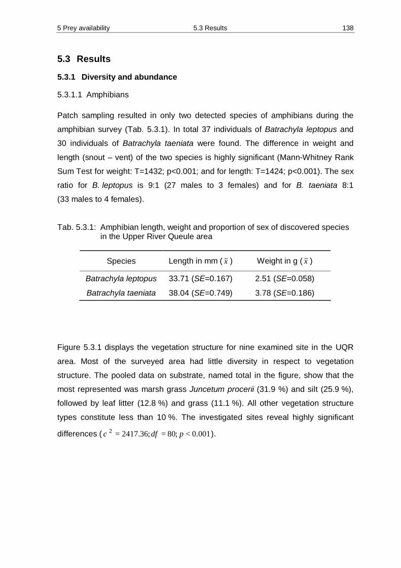
5 Prey availability 5.3 Results 138
5.3 Results
5.3.1 Diversity and abundance
5.3.1.1 Amphibians Patch sampling resulted in only two detected species of amphibians during the
amphibian survey (Tab. 5.3.1). In total 37 individuals of Batrachyla leptopus and
30 individuals of Batrachyla taeniata were found. The difference in weight and
length (snout – vent) of the two species is highly significant (Mann-Whitney Rank
Sum Test for weight: T=1432; p<0.001; and for length: T=1424; p<0.001). The sex
ratio for B. leptopus is 9:1 (27 males to 3 females) and for B. taeniata 8:1
(33 males to 4 females).
Tab. 5.3.1: Amphibian length, weight and proportion of sex of discovered species in the Upper River Queule area
Species Length in mm ( x ) Weight in g ( x )
Batrachyla leptopus 33.71 (SE=0.167) 2.51 (SE=0.058)
Batrachyla taeniata 38.04 (SE=0.749) 3.78 (SE=0.186)
Figure 5.3.1 displays the vegetation structure for nine examined site in the UQR
area. Most of the surveyed area had little diversity in respect to vegetation
structure. The pooled data on substrate, named total in the figure, show that the
most represented was marsh grass Juncetum procerii (31.9 %) and silt (25.9 %),
followed by leaf litter (12.8 %) and grass (11.1 %). All other vegetation structure
types constitute less than 10 %. The investigated sites reveal highly significant
differences ( 001.0;80;36.24172 <== pdfχ ).

5 Prey availability 5.3 Results 139
0
10
20
30
40
50
60
70
80
90
100
1 2 3 4 5 6 7 8 9 Total
Site
Subs
trat
e (%
)Big TreesTreesBushesRootsLogsHerbsGrassMarsh grassLeaf litterSiltSand/Stones
(8/4) (0/8) (6/1) (7/4) (0/3) (5/1) (0/0) (4/3) (7/6)
Fig. 5.3.1: Substrate composition of nine explored sites; (x/y) = abundance of
Batrachyla leptopus and Batrachyla taeniata
The dendogram (Fig. 5.3.2) shows that the Euclidean distance from the main used
substrate swamp grass to the other clusters, leaf litter, grass and silt, is highest.
The substrates grass and silt build a cluster because they were used less
frequently.
Swamp grass Leaf litter Grass Silt
Substrate
0
10
20
30
40
50
60
70
80
90
100
Euc
lidea
n di
stan
ce
Fig. 5.3.2: Dendogram of used substrate by two species of the genus Batrachyla

5 Prey availability 5.3 Results 140
B. leptopus is using four out of 11 available vegetation structures as displayed in
Figure 5.3.3. The structure forms most commonly inhabited by B. leptopus are the
variable marsh grass with a standardized selection index (Bi) of 0.486 and leaf
litter with 0.387. The other two variables, silt (0.072) and grass (0.056) do not
present a common selected vegetation substrate. The second identified species
B. taeniata inhabited only three substrate types of vegetation consisting of marsh
grass (0.606), by leaf litter (0.329), and silt (0.065). A high niche overlap exists
between B. leptopus and B. taeniata (RO = 0.982; Horn’s index of similarity). The
Levins’s standardized niche breadth for B. leptopus and B. taeniata is 0.319 and
0.307 respectively. Both species frequently use three resources (substrates).
0
0,1
0,2
0,3
0,4
0,5
0,6
0,7
0,8
0,9
1
B. leptopus B. taeniata
Species
Inde
x (B
i)
Big Trees Trees Bushes Roots LogsHerbsGrass Marsh grass Leaf litter Silt Sand/Stones
Fig. 5.3.3: Standardized selection index (Bi); vegetation structure where amphibian
species were discovered
Strait-line drift fences with pitfall traps were set over 14 days on different locations
and in different vegetation structure types. No amphibians were captured during
this time span using this method.
Two further species, Caudiverbera caudiverbera and Pleurodema thaul were
discovered occasionally crossing gravel roads and during telemetry studies on
Lontra provocax.

5 Prey availability 5.3 Results 141
5.3.1.2 Fish and Crustaceans By using the “red de palito” gear, two species of crustaceans were discovered
(Fig. 5.3.4 a). The majority of the crustaceans were found in the riverbed
structures woody debris (75.5 %) by gravel (16.0 %) and stones (5.5 %). In the
substrate sand only Samastacus spinifrons (3.1 %) was collected, whereas the
substrate rock was without any findings.
Stop-net was used while electrofishing to prevent fish from escaping and
crustacean for being flushed away with the current. However, the stop-net was
insufficient for crustacean and fish smaller than 10 mm . While electro stunned fish
was collected easily and swam into the spoon net, crustacean moved their pleon
pulsative and “swam” to the water surface area, where it had to be caught
immediately for not be carried away by the current. Using electrofishing gear, not
only were four species of fish discovered, additionally the total abundance in
crustaceans increased (Fig. 5.3.4 b). The total number of discovered crustaceans
is three times higher (75.7 %) than it was when collected with the first described
method (24.3 %). In general the “red de palito”- method discovered 22.3 % out of
740 individuals and 33.3 % out of six species. Interestingly the most undetected
crustaceans were found in the riverbed substrate woody debris. Fish were present
in sand, gravel, stones and woody debris but absent in the substrate rocks. The
species similarity index was relatively high between the two investigated methods
(Soerensen’s similarity coefficient Ss = 0.750).
Eleven sections were examined with electrofishing gear in 2003 and five sections
in 2004. Ten of these sections were located in the UQR (four in 2004) and one
section in the near by Mahuidanche (one in 2004) river for comparison. In total
eleven species were discovered using electrofishing. In Table 5.3.2 the scientific
names, common names and the status of each located species are described. The
riverbed structure was classified into seven categories: sand, gravel, stones,
rocks, woody debris, trees/roots and aquatic plants (Appendix 10.4; Tab. C). The
presence for the most common substrate types was 90.1 % for woody debris and
81.8 % for sand. The substrate aquatic plant was only found in section eleven and
therefore displays the lowest presence with 9.1 %. Within the species,
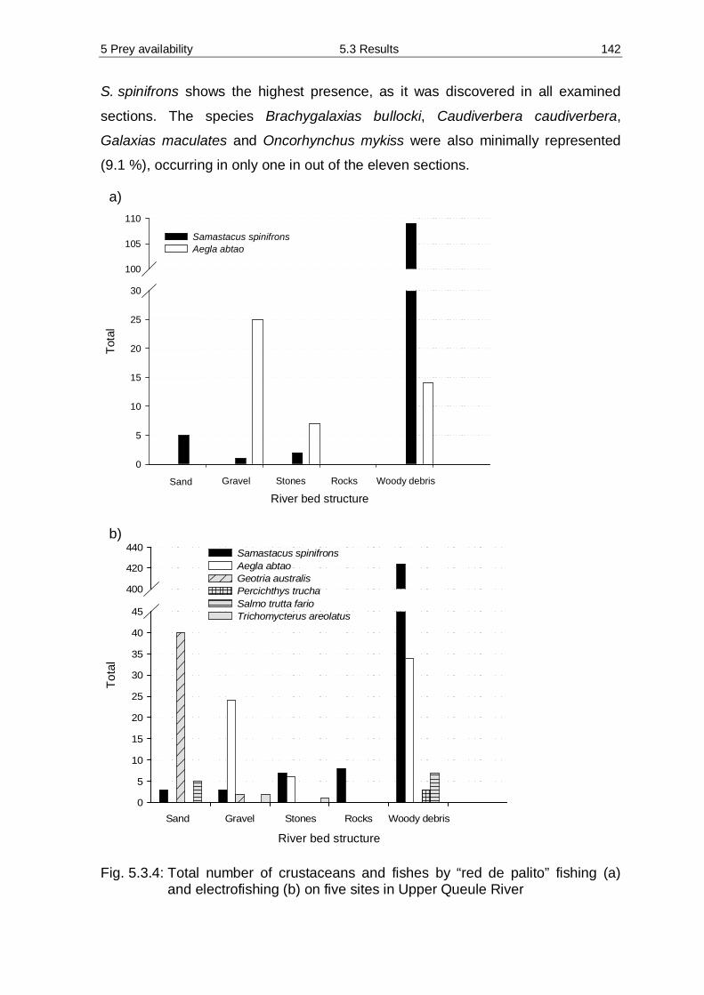
5 Prey availability 5.3 Results 142
S. spinifrons shows the highest presence, as it was discovered in all examined
sections. The species Brachygalaxias bullocki, Caudiverbera caudiverbera,
Galaxias maculates and Oncorhynchus mykiss were also minimally represented
(9.1 %), occurring in only one in out of the eleven sections.
River bed structure
Sand Gravel Stones Rocks Woody debris
Tota
l
0
5
10
15
20
25
30
100
105
110
Samastacus spinifrons Aegla abtao
Sand Gravel Stones Rocks Woody debris
River bed structure
Sand Gravel Stones Rocks Woody debris
Tota
l
0
5
10
15
20
25
30
35
40
45
400
420
440 Samastacus spinifronsAegla abtaoGeotria australis Percichthys trucha Salmo trutta fario Trichomycterus areolatus
Sand Gravel Stones Rocks Woody debris
Fig. 5.3.4: Total number of crustaceans and fishes by “red de palito” fishing (a)
and electrofishing (b) on five sites in Upper Queule River
b)
a)
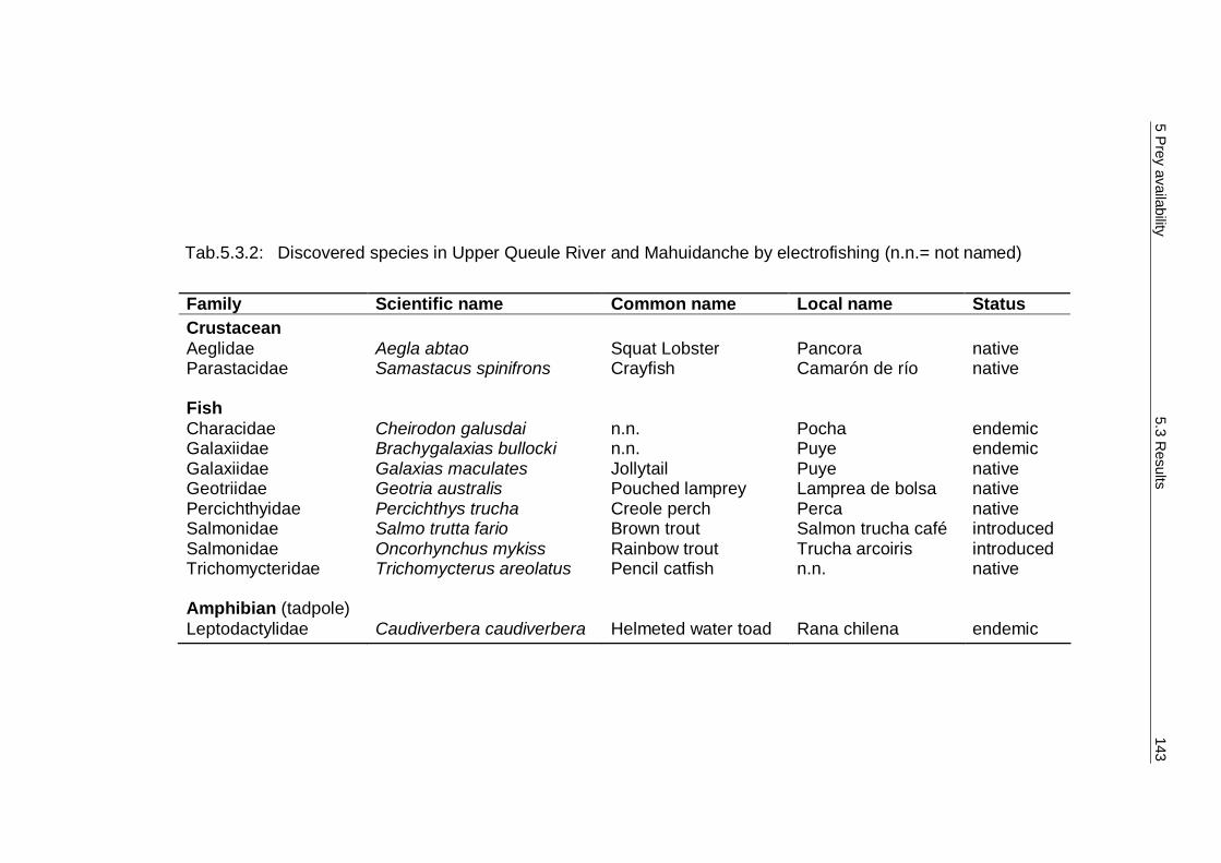
5 Prey availability
5.3 Results
143
Tab.5.3.2: Discovered species in Upper Queule River and Mahuidanche by electrofishing (n.n.= not named)
Family Scientific name Common name Local name Status Crustacean Aeglidae Aegla abtao Squat Lobster Pancora native Parastacidae Samastacus spinifrons Crayfish Camarón de río native Fish Characidae Cheirodon galusdai n.n. Pocha endemic Galaxiidae Brachygalaxias bullocki n.n. Puye endemic Galaxiidae Galaxias maculates Jollytail Puye native Geotriidae Geotria australis Pouched lamprey Lamprea de bolsa native Percichthyidae Percichthys trucha Creole perch Perca native Salmonidae Salmo trutta fario Brown trout Salmon trucha café introduced Salmonidae Oncorhynchus mykiss Rainbow trout Trucha arcoiris introduced Trichomycteridae Trichomycterus areolatus Pencil catfish n.n. native Amphibian (tadpole) Leptodactylidae Caudiverbera caudiverbera Helmeted water toad Rana chilena endemic

5 Prey availability 5.3 Results 144
The riverbed structure composition of each surveyed site is displayed in Fig. 5.3.5.
Other than site Q 03, which only consists of sand, all examined sites include more
than one riverbed structure variable. It should be noted that the riverbed structure
in the UQR does not contain aquatic plants, whereas site M 01 in Mahuidanche
River consists 95 % of aquatic plants and 5 % of woody debris. The main riverbed
structure component (Q total) is more diverse in the UQR, whereby sand (37 %),
gravel (29 %), and woody debris (22 %) dominated the structure variables. All
other structure variables were present under 10 %.
0
10
20
30
40
50
60
70
80
90
100
Q 01 Q 02 Q 03 Q 04 Q 05 Q 06 Q 07 Q 08 Q 09 Q 10 M 01 Q total
Site
Riv
er b
ed s
truc
ture
(%)
Aquatic plantsTrees / rootsWoody debrisRocksStonesGravelSand
Fig. 5.3.5: River bed substrate composition of the electrofished area (Q = Queule River; M = Mahuidanche River)

5 Prey availability 5.3 Results 145
The dissimilarity of species community of the examined sites is shown as a
dendogram in Fig. 5.3.6. All investigated river sections branch further into several
clusters but the separated site M 01, which displays the only analysed section in
the Mahuidanche River. In this river section most aquatic species (9) were
discovered.
M 01 Q 08 Q 09 Q 04 Q 07 Q 06 Q 02 Q 05 Q 10 Q 03 Q 010,2
0,3
0,4
0,5
0,6
0,7
0,8
0,9
1,0
Dis
sim
ilarit
y
Fig. 5.3.6: Tree diagram resulting from an unweighted pair-group average cluster analysis of river species community (Appendix 10.4; Tab. C); (Q = Queule River; M = Mahuidanche River)
It should be noted that of the eleven electrofished sites only sites Q 02 and Q 07
have a Simpson’s diversity index (1-D) higher than 0.4 (Fig. 5.3.7). The lowest
diversity index was found in site Q 10 with 1-D = 0.04. Likewise the evenness has
a high variance between the examined sites. The highest Smith and Wilson’s
index of evenness (Evar) was found in site Q 01 with Evar = 0.39. The lowest Evar
was found in site Q 10 with 0.16. On average the Simpson’s diversity index for the
UQR is 0.26 and the Evar averages 0.25. Whereas 1- D is 0.20 and Evar is 0.17 for
the Mahuidanche River site (M 01). No correlation was found between species
diversity and substrate diversity (rs= 0.0727; p=0.818).

5 Prey availability 5.3 Results 146
Site
Q 01 Q 02 Q 03 Q 04 Q 05 Q 06 Q 07 Q 08 Q 09 Q 10 M 01
Inde
x
0,0
0,1
0,2
0,3
0,4
0,5
0,6
Simpson´s index of diversity (1-D)Smith and Wilson´s index of eveness (Evar)
(114) (210) (18) (166) (198) (77) (81) (330) (85) (50) (690)
Fig. 5.3.7: Diversity and evenness indices are listed for all electrofished areas. Total number of caught individuals is displayed in parentheses (Q = Queule River; M = Mahuidanche River)
The average weight of electrofished species within the 11 examined sites is
displayed in Fig. 5.3.8. The weight of species differed significantly in the median
values among the groups (ANOVA on Ranks; H=369.066; df=10; p<0.001).
However, the adjacent all pairwise multiple comparison procedures (Dunn’s
Method) did not detect any significant difference. The highest median in weight is
shown by Oncorhynchus mykiss ( 55.9;45.40~ == SEx ) and the tadpole
Caudiverbera caudiverbera ( 60.3;90.11~ == SEx ). For all other species the median
is lower than 2.5 g. The highest range was found in S. spinifrons (51.32 g) and
Salmo trutta fario (179.90 g); however these values are not displayed, as only the
first outliers that lie outside the 10th and 90th percentile are shown.

5 Prey availability 5.3 Results 147
Species
A.a. S.s. B.b. C.c. C.g. G.a. G.m. O.m. P.t. S.t.f. T.a
Wei
ght (
g)
0
5
10
15
2040
45
(206) (1243) (20) (6) (134) (568) (2) (69)(2) (8) (6)
Fig. 5.3.8: Average weight of captured species by electrofishing. (x) = number of
individuals; A.a. = Aegla abtao; S.s. = Samastacus spinifrons; B.b. = Brachygalaxias bullocki; Caudiverbera caudiverbera; C.g. = Cheirodon galusdai; G.a. = Geotria australis; G.m. = Galaxias maculates; O.m. = Oncorhynchus mykiss; P.t. = Percichthys trucha; S.t.f. = Salmo trutta fario; T.a. = Trichomycterus areolatus
The dominance structures of discovered species using electrofishing are displayed
separately in Fig. 5.3.9 a, b for the UQR and the Mahuidanche River.
Samastacus spinifrons present with 81.7 % the eudominant species in the Upper
River Queule and is presented with A. abtao and Geotria australis, the stock
forming species. The other fish species are by definition companions which are not
markedly associated with this community and are represented by less than 3.2 %.
In the Mahuidanche River Galaxias maculates forms the eudominant species with
89 %. Here, the crustacean species S. spinifrons and A. abtao are only
subdominant, but still represent the stock forming species. Two more species are
listed in the Mahuidanche than in the UQR section, but these are only companion
species.

5 Prey availability 5.3 Results 148
0,2
0,3
0,5
2,0
6,1
9,3
81,7
0 10 20 30 40 50 60 70 80 90 100
Cheirodon galusdai
Percichthys trucha
Trichomycerus areolatus
Salmo trutta fario
Geotria australis
Aegla abtao
Samastacus spinifrons
stock forming species
0,1
0,3
0,3
0,3
0,3
2,9
3,2
3,6
89,0
0 10 20 30 40 50 60 70 80 90 100
Trichomycterus areolatus
Cheirodon galusdai
Oncorhynchus mykiss
Salmo trutta fario
Caudiverbera caudiverbera
Brachygalaxias bullocki
Geotria australis
Samastacus spinifrons
Galaxias maculates
stock forming species
Dominance classes 32.00 - 100.00 % eudominant 10.00 - < 32.00 % dominant 3.20 - < 10.00 % subdominant 1.00 - < 3.20 % recedent 0.32 - < 1.00 % subrecedent < 0.32 % sporadic
Dominance classes 32.00 - 100.00 % eudominant 10.00 - < 32.00 % dominant 3.20 - < 10.00 % subdominant 1.00 - < 3.20 % recedent 0.32 - < 1.00 % subrecedent < 0.32 % sporadic
a)
b)
Fig. 5.3.9: Dominance structure for UQR (a) and for Mahuidanche River (b)
(Queule River describes 10 sections, Mahuidanche River describes one section)
Within the electrofished samples, two introduced fish species, Salmo trutta fario
and Oncorhynchus mykiss, were identified. As Fig. 5.3.10 displays, these species
have different influence in the community composition. In the Upper Queule River
27 of 119 captured fish were Salmon trutta fario, whereas in the Mahuidanche
electrofished site two Salmon trutta fario and additional two Oncorhynchus mykiss
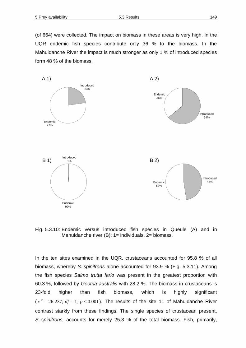
5 Prey availability 5.3 Results 149
Introduced64%
Endemic36%
Introduced1%
Endemic99%
Introduced48%Endemic
52%
Introduced23%
Endemic77%
(of 664) were collected. The impact on biomass in these areas is very high. In the
UQR endemic fish species contribute only 36 % to the biomass. In the
Mahuidanche River the impact is much stronger as only 1 % of introduced species
form 48 % of the biomass.
Fig. 5.3.10: Endemic versus introduced fish species in Queule (A) and in
Mahuidanche river (B); 1= individuals, 2= biomass.
In the ten sites examined in the UQR, crustaceans accounted for 95.8 % of all
biomass, whereby S. spinifrons alone accounted for 93.9 % (Fig. 5.3.11). Among
the fish species Salmo trutta fario was present in the greatest proportion with
60.3 %, followed by Geotria australis with 28.2 %. The biomass in crustaceans is
23-fold higher than fish biomass, which is highly significant
( 001.0;1;237.262 <== pdfχ ). The results of the site 11 of Mahuidanche River
contrast starkly from these findings. The single species of crustacean present,
S. spinifrons, accounts for merely 25.3 % of the total biomass. Fish, primarily,
B 1)
A 2) A 1)
B 2)

5 Prey availability 5.3 Results 150
265.1 265.1
12.8
3.5
375.0
17.7
80.9
290.0
780.7
1.0
10.0
100.0
1000.0
10000.0
Samastacu
s spinifro
ns
Brach
ygalaxia
s bullo
cki
Cheirodon g
alusdai
Galaxias m
aculatus
Geotria aus
tralis
Oncorh
ynch
us m
ykiss
Salmo t
rutta
f.
Tricho
mycteru
s are
olatus
Total C
rustace
an
Total F
ish
Species
Wei
ght i
n gr
am (l
og)
CrustaceanFish
0.8
80,0
4038,9 4118,9
6,7
50,9
3,0
108,9
11,1
180,6
1,0
10,0
100,0
1000,0
10000,0
Aegla abtao
Samastacu
s spin
ifrons
Cheirodo
n galusd
ai
Geotria
austr
alis
Percich
thys t
rucha
Salmo tr
utta f.
Trichomyc
terus areolatus
Total C
rustace
an
Total F
ish
Species
Wei
ght i
n gr
am (l
og)
CrustaceanFish
Galaxias maculates and Salmo trutta fario, produce the principal part with 74.6 %.
The biomass in fish on this site is 3-fold higher than crustacean biomass. The
difference between crustacean and fish was not tested due to low number of
cases within the crustaceans.
a)
b)
Fig. 5.3.11: Biomass of (a) Upper Queule River (10 sections) and (b) Mahuidanche
River 2003 (1 section)
Partitioning species based on the riverbed substrate in which they are found
reveals that species richness is highest in aquatic plants (8) where all species but
A. abtao and Percichthys trucha are present (Fig. 5.3.12). On this substrate
Galaxias maculates forms the eudominant species with 89.4 %. Woody debris

5 Prey availability 5.3 Results 151
follows with six species; S. spinifrons (92.2 %) and A. abtao (5.3 %) being
dominant. Five species are present in the gravel substrate; the dominant being
A. abtao with 74.6 % followed by S. spinifrons with 16.9 %. Four species are
present in the substrate trees/roots, where S. spinifrons is the dominant species
with 94.6 % followed by Salmo trutta f. with 3.6 %. The same species richness (3)
is found in the substrates stones and sand. In the riverbed structure stones
crustaceans form the dominant species, A. abtao with 53.6 % and S. spinifrons
with 42.9 % respectively. In contrast Geotria australis, with 81.3 %, was the
dominant species in sand. Only S. spinifrons was found in the substrate rocks
(100 %). The Kruskal – Wallis ANOVA on Ranks did no show any significant
statistical differences between the riverbed structure and number of individuals
found (H=11.424, df=6; p=0.076).
0.1
1.0
10.0
100.0
1000.0
SAND GRAVEL STONES ROCKS WOODY DEBRIS TREES / ROOTS AQUATIC PLANTS
Substrate
Tota
l (lo
g)
Aegla abtao Samastacus spinifrons Caudiverbera caudiverbera Geotria australisPercichthys trucha Cheirodon galusdai Salmo trutta f. Trichomycterus areolatusGalaxias maculates Brachygalaxias bullocki Oncorhynchus mykiss
Fig. 5.3.12: Occurrence of species in river bed structure by electrofishing in Upper
Queule River and Mahuidanche River 2003 (electrofished areas n=11, species n=11; total n=2013)
The standardized selection index (Bi) shows that A. abtao preferred the river bed
substrate stones (Bi = 0.438), followed by woody debris (Bi = 0.300) and gravel
(Bi = 0.238) (Fig. 5.3.13.). Levins’s measure of standardized niche breadth (BA) is

5 Prey availability 5.3 Results 152
0.515 and the number of frequently used resource constitutes 3 (Appendix 10.4;
Tab. A). For S. spinifrons substrates woody debris (Bi = 0.597), and trees/roots
(Bi = 0.255) are most important, whereas rocks (Bi = 0.056), stones (Bi = 0.044)
and aquatic plants (Bi = 0.037) are from minor significance. S. spinifrons uses two
resources/substrates frequently. The BA value is 0.065.
0.0
0.1
0.2
0.3
0.4
0.5
0.6
0.7
0.8
0.9
1.0
A.a. S.s B.b. C.c. C.g. G.m. G.a. O.m. P.t. S.t.f. T.a.
Species
Inde
x (B
i)
Aquatic plantsTrees/rootsWoody debrisRocksStonesGravelSand
Fig. 5.3.13: Standardized selection index (Bi); river bed structure where species
were electro stunned; A.a. = A. abtao; S.s. = Samastacus spinifrons; B.b. = Brachygalaxias bullocki; C.c. = Caudiverbera cuadiverbera; C.g. = Cheirodon galusdai; G.a. = Geotria australis; G.m. = Galaxias maculates; O.m. = Oncoryhnchus mykiss; P.t. = Percichthys trucha; S.t.f. = Salmo trutta fario; T.a. = Trichomycterus areolatus
The species Brachygalaxias bullocki, Galaxias maculates, Oncorhynchus mykiss
and Caudiverbera caudiverbera were only found on site 11 in Mahuidanche River
in the substrate aquatic plants. Two other species Cheirodon galusdai and
Percichthys trucha were also found in only one substrate, in woody debris. Due to
this fact, Bi is 1.00 and BA was not calculated. Geotria australis favourite aquatic
plants (Bi = 0.508) a little bit more compared to sand (Bi = 0.477). The BA results in
0.298 and the number of frequency used resources composes two. However, it
has to be considered, that the bottom substrate of aquatic plants consists of sand.

5 Prey availability 5.3 Results 153
Woody debris (Bi = 0.415) and trees/roots (Bi = 0.387) are preferred by Salmo
trutta fario, followed by aquatic plants (Bi = 0.108) and sand (Bi = 0.071). Four
substrates are frequently used by Salmo trutta fario which BA is 0.357. The Bi
values for Trichomycterus areolatus were highest for stones (Bi = 0.345) and much
lower for gravel (Bi = 0.159) followed by trees/roots (Bi = 0.276) and aquatic plants
(Bi = 0.153), whereas the substrate woody debris has the lowest value
(Bi = 0.066). Levins’s measure of standardized niche breadth for Trichomycterus
areolatus is 0.669 and it frequently used 5 substrates. The difference in the river
bed structure composition for each species is highly significant
( 001.0;60;18.22252 <==ℵ pdf ).
For the purpose of comparison electrofishing was carried out in 2003 and 2004 on
five similar sites. The difference of abundance and weighted biomass is shown in
Tab. 5.3.3. Ten days before the five sites were examined in 2004 heavy rain
produced flooding. The differences between total catches and biomass in 2003 and 2004 are highly significant ( 001.0;10;792.3592 <== pdfχ )
( 001.0;10;439.1842 <== pdfχ ). The proportion of the abundance of the
crustaceans A. abtao to S. spinifrons in 2003 was 11 % to 89 % which changed to
31 % to 69 % in 2004 following the flooding. This difference is highly significant ( 001.0;1;342.562 <== pdfχ ). Furthermore the difference for fish between 2003
and 2004 was also highly significant ( 001.0;14;291.4472 <== pdfχ ) which was
mainly attributed to the absence of Galaxias maculates, which had a strong
influence on the samples of 2003 versus 2004 (85.77 %, entirety of column;
99.84 %, entirety of row). Riverbed structures in the some section changed in
2004 due to flooding and strong current.

5 Prey availability 5.3 Results 154
Tab. 5.3.3: Total abundance and biomass of five electrofished sections in 2003 and 2004 after flood
Total Biomass (g)
Species 2003 2004 2003 2004
Crustaceans (Σ) (710) (262) (3537.9) (801.8) Aegla abtao 79 82 116.6 64.4 Samastacus spinifrons 631 180 3421.3 737.4 Fish (Σ) (717) (65) (1036.7) (150.1) Brachygalaxias bullocki 20 0 12.8 0.0 Cheirodon galusdai 4 1 10.3 0.1 Galaxias maculates 615 0 375.0 0.0 Geotria australis 50 26 60.0 20.2 Oncorhynchus mykiss 2 0 80.9 0.0 Percichthys trucha 1 4 19.9 19.7 Salmo trutta fario 20 34 469.7 110.1 Trichomycterus areolatus 5 0 8.1 0.0 Amphibians (tadpole) (Σ) (2) (0) (23.8) (0.0) Caudiverbera caudiverbera 2 0 23.8 0.0
Total 1429 327 4574.6 951.9
5.3.2 Spraint analysis
5.3.2.1 Lontra provocax
Over a time span of 17 months an average of 13 (SE=1.49) spraint sites used by
southern river otters in the UQR were discovered, whereby the minimum of six
sites were detected in April 2003 and the maximum of 29 sites were found in
August 2003 (Fig. 5.3.14). The averaged number of faeces samples collected per
month was 37.2 (SE=7.3). The minimum number of faeces samples occurred in
December 2006 with nine samples and the maximum in August 2003 with 132
samples. There is a strong correlation between sprainting sites and number of
faeces sampled (rs=0.746; p<0.001).

5 Prey availability 5.3 Results 155
0
20
40
60
80
100
120
140
JAN03
F M A M J J A S O N D JAN04
F M A M J J
Month
Qua
ntity
SpraintsSites
Fig. 5.3.14: Quantity of spraint sites and spraints on the Queule Upper River
(n=630 spraints)
Little precipitation was noted in the Queule River area between January and May,
where precipitation events never exceed 100 mm (Tab. 5.3.4). From August
through September moderate precipitation (100 – 250 mm) was recorded, though
the months of June and July received the most precipitation. The lowest number of
faeces samples was collected in months with low precipitation, whereas months of
high precipitation provided more faeces samples in 2003. The numbers of low
precipitation in 2004 are similar to 2003; however there is a difference in faeces
samples between 2003 and 2004 when highest precipitation occurred. The
difference between collected faecal samples in lowest and highest precipitation
seasons is insignificant (One-Way ANOVA: F = 1.399; df = 16; p = 0.279).
Tab. 5.3.4: Precipitation and average numbers of otter faeces
Precipitation Low
(< 100 mm)
Medium
(100 – 250 mm )
High
(> 250 mm )
2003 26.6 53.6 52
2004 24 --- 27
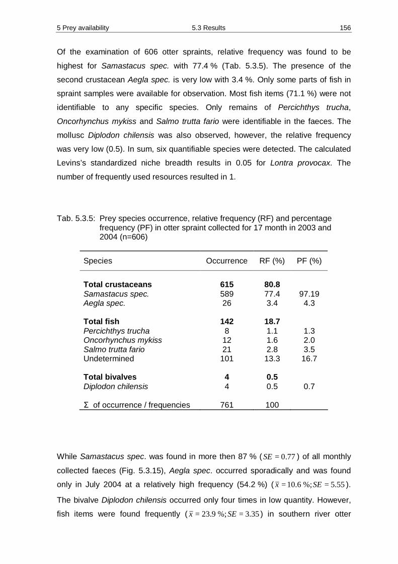
5 Prey availability 5.3 Results 156
Of the examination of 606 otter spraints, relative frequency was found to be
highest for Samastacus spec. with 77.4 % (Tab. 5.3.5). The presence of the
second crustacean Aegla spec. is very low with 3.4 %. Only some parts of fish in
spraint samples were available for observation. Most fish items (71.1 %) were not
identifiable to any specific species. Only remains of Percichthys trucha,
Oncorhynchus mykiss and Salmo trutta fario were identifiable in the faeces. The
mollusc Diplodon chilensis was also observed, however, the relative frequency
was very low (0.5). In sum, six quantifiable species were detected. The calculated
Levins’s standardized niche breadth results in 0.05 for Lontra provocax. The
number of frequently used resources resulted in 1.
Tab. 5.3.5: Prey species occurrence, relative frequency (RF) and percentage frequency (PF) in otter spraint collected for 17 month in 2003 and 2004 (n=606)
Species Occurrence RF (%) PF (%)
Total crustaceans 615 80.8 Samastacus spec. 589 77.4 97.19 Aegla spec. 26 3.4 4.3 Total fish 142 18.7 Percichthys trucha 8 1.1 1.3 Oncorhynchus mykiss 12 1.6 2.0 Salmo trutta fario 21 2.8 3.5 Undetermined 101 13.3 16.7 Total bivalves 4 0.5 Diplodon chilensis 4 0.5 0.7 Σ of occurrence / frequencies 761 100
While Samastacus spec. was found in more then 87 % ( 77.0=SE ) of all monthly
collected faeces (Fig. 5.3.15), Aegla spec. occurred sporadically and was found
only in July 2004 at a relatively high frequency (54.2 %) ( 55.5%;6.10 == SEx ).
The bivalve Diplodon chilensis occurred only four times in low quantity. However,
fish items were found frequently ( 35.3%;9.23 == SEx ) in southern river otter
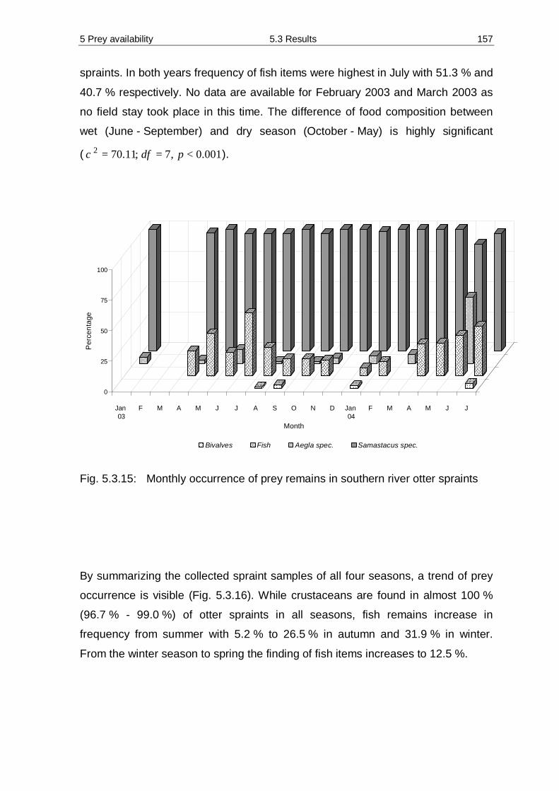
5 Prey availability 5.3 Results 157
spraints. In both years frequency of fish items were highest in July with 51.3 % and
40.7 % respectively. No data are available for February 2003 and March 2003 as
no field stay took place in this time. The difference of food composition between
wet (June - September) and dry season (October - May) is highly significant
( 001.0,7;11.702 <== pdfχ ).
0
25
50
75
100
Per
cent
age
Jan 03
F M A M J J A S O N D Jan 04
F M A M J J
Month
Bivalves Fish Aegla spec. Samastacus spec.
Fig. 5.3.15: Monthly occurrence of prey remains in southern river otter spraints
By summarizing the collected spraint samples of all four seasons, a trend of prey
occurrence is visible (Fig. 5.3.16). While crustaceans are found in almost 100 %
(96.7 % - 99.0 %) of otter spraints in all seasons, fish remains increase in
frequency from summer with 5.2 % to 26.5 % in autumn and 31.9 % in winter.
From the winter season to spring the finding of fish items increases to 12.5 %.

5 Prey availability 5.3 Results 158
Seasons
Summer Autumn Winter Spring
Perc
enta
ge o
f pre
y oc
curr
ence
0
50
100
CrustaceansFish
Fig. 5.3.16: Seasonal frequency of prey remains in otter spraint
Stomach content
The stomach content of two southern river otter was examined. The other otter
which died in captivity was not used for further analysis as it was only fed fish.
The male subadult – adult southern river otter was from the UQR, whereas the
female adult southern river otter was found in the River Cruces (close to Valdivia).
Stomach and intestine were rinsed thoroughly and prey items were identified. In
both sexes only the crustacean species S. spinifrons was detected and no fish
remains.
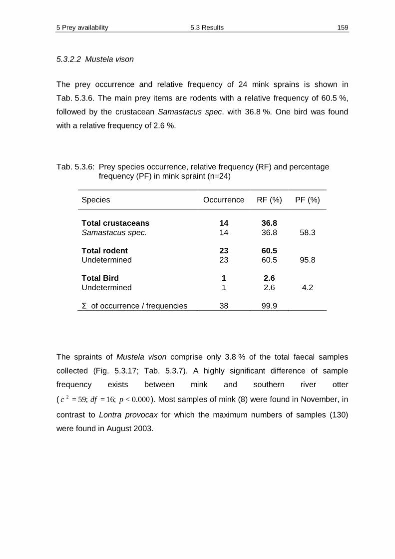
5 Prey availability 5.3 Results 159
5.3.2.2 Mustela vison
The prey occurrence and relative frequency of 24 mink sprains is shown in
Tab. 5.3.6. The main prey items are rodents with a relative frequency of 60.5 %,
followed by the crustacean Samastacus spec. with 36.8 %. One bird was found
with a relative frequency of 2.6 %.
Tab. 5.3.6: Prey species occurrence, relative frequency (RF) and percentage frequency (PF) in mink spraint (n=24)
Species Occurrence RF (%) PF (%)
Total crustaceans 14 36.8 Samastacus spec. 14 36.8 58.3 Total rodent 23 60.5 Undetermined 23 60.5 95.8 Total Bird 1 2.6 Undetermined 1 2.6 4.2 Σ of occurrence / frequencies 38 99.9
The spraints of Mustela vison comprise only 3.8 % of the total faecal samples
collected (Fig. 5.3.17; Tab. 5.3.7). A highly significant difference of sample
frequency exists between mink and southern river otter
( 000.0;16;592 <== pdfχ ). Most samples of mink (8) were found in November, in
contrast to Lontra provocax for which the maximum numbers of samples (130)
were found in August 2003.

5 Prey availability 5.3 Results 160
Month
Tota
l (lo
g)
0,1
1
10
100
1000
Mustela vison Lontra provocax
J03
F M A M J J A S O N D J04
F M A M J J Total
Fig. 5.3.17: Monthly occurrence of mink and southern river otter spraints The species richness found in spraint samples of Mustela vison was 50 % as great
as those of southern river otters (Tab. 5.3.7). In contrast to this, the diversity
indices Shannon-Wiener and Simpson as well as the Smith and Wilson index for
evenness were higher for mink. The Renkonen-Index for similarity of food
resources between determined food items in faeces samples of mink and southern
river otter is Re = 36.84 %.
Tab. 5.3.7: Diet diversity from spraints collected on the Queule river 2003 – 2004
(H´ - Shannon – Wiener Diversity Index; (1-D) = Simpson’s diversity index)
Index Lontra provocax Mustela vison Total Abundance 606 > 24 Species Richness 6 > 3
Shannon’s H´ 0.496 < 0.768 Simpson (1-D) 0.201 < 0.511
Smith and Wilson’s Evar 0.240 < 0.309

5 Prey availability 5.3 Results 161
5.3.3 Prey availability versus diet composition
Relative frequencies of available prey species found in the UQR and detected in
faecal samples are compared in Tab. 5.3.8. Prey abundances were calculated
using data from electrofishing only in 2003, whereas the abundance of prey in
faecal samples includes all collected samples during 2003 to 2004. No correlation
was detected between prey availability and diet composition (rS = 0.537; p > 0.05).
This is due to the absence of the fish species Ch. galusdai, G. australis and
T. areolatus in faecal samples. In contrast to the ranked fish species, which show
no similarity in ranking order (except Ch. galusdai), the rank order of crustaceans
is identical. Unidentified fish were not considered in ranking. The Renkonen-Index,
which measures similarity between the aquatic species composition and the
dietary composition of L. provocax is calculated as Re = 83.7 %.
Tab. 5.3.8: Relative frequency (RF) of collected aquatic animals in river versus detected in faeces of the southern river otter. Rank order in brackets
Species in river (RF) in faeces
(RF)
Total crustaceans 91.0 81.2 Samastacus spec. 81.7 (1) 77.8 (1) Aegla spec. 9.3 (2) 3.4 (2) Total fish 9.1 18.7 Percichthys trucha 0.3 (6) 1.1 (5) Oncorhynchus mykiss 0.0 (8) 1.6 (4) Salmo trutta fario 2.0 (4) 2.8 (3) Cheirodon galusdai 0.2 (7) 0.0 (7) Geotria australis 6.1 (3) 0.0 (7) Trichomycterus areolatus 0.5 (5) 0.0 (7) Undetermined* 0.0 13.0 Total 100.1 99.9
* not considered in rank order

5 Prey availability 5.3 Results 162
0 20 40 60 80 100 120 140
Total length (mm)
-2
0
2
4
6
8
10
12
14
16
18
20
Leng
th o
f Ros
trum
(mm
)
-3 -2 -1 0 1 2 3 4 5
Weight (g)(ln-transformed)
2,22,42,62,83,03,23,43,63,84,04,24,44,64,85,0
Tota
l len
gth
(mm
)(ln
-tran
sfor
med
)
-3,0 -2,5 -2,0 -1,5 -1,0 -0,5 0,0 0,5 1,0 1,5 2,0
Weight (g)(ln-transformed)
0,2
0,4
0,6
0,8
1,0
1,2
1,4
1,6
1,8
2,0
2,2
2,4
2,6
Leng
th o
f Ros
trum
(mm
)(ln
-tran
sfor
med
)
-3,0 -2,5 -2,0 -1,5 -1,0 -0,5 0,0 0,5 1,0 1,5 2,0
Weight (g)(ln-transformed)
-0,5
0,0
0,5
1,0
1,5
2,0
2,5
3,0
3,5
4,0
Leng
th o
f Cep
halo
thor
ax (m
m)
(ln-tr
ansf
orm
ed)
-3 -2 -1 0 1 2 3 4 5
Weight (g)(ln-transformed)
-0,5
0,0
0,5
1,0
1,5
2,0
2,5
3,0
3,5
Leng
th o
f Ros
trum
(mm
)(ln
-tran
sfor
med
)
-5 0 5 10 15 20 25 30 35
Length of Cephalothorax (mm)
0
1
2
3
4
5
6
7
8
Leng
th o
f Ros
trum
(mm
)
5.3.4 Required quantity of staple prey
The weight, rostrum length, and total length of crustaceans caught by
electrofishing were measured. Fig. 5.3.18 presents the linear regression of rostrum
length to total length, rostrum length to weight (log transformed), and total length
to weight (log transformed) for the crustacean species S. spinifrons and A. abtao.
Fig. 5.3.18: Correlation of rostrum and total length of (a) Samastacus spinifrons
(n=1242) and (b) Aegla abtao (n=190)
a) b)
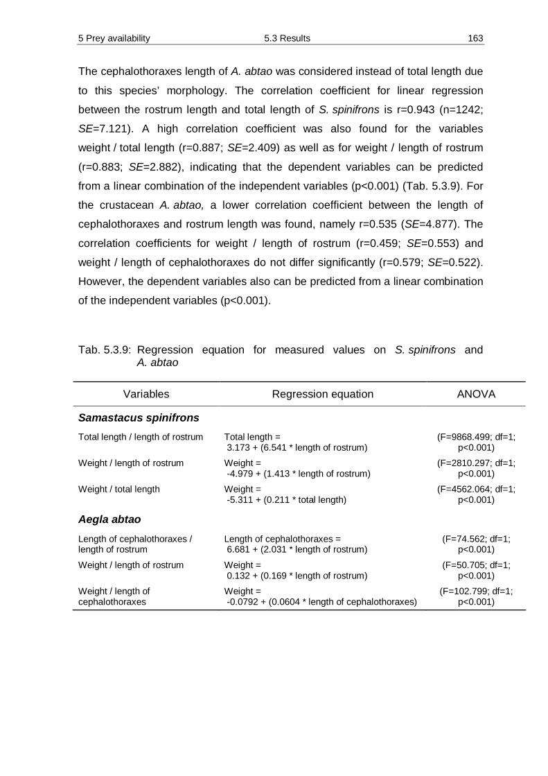
5 Prey availability 5.3 Results 163
The cephalothoraxes length of A. abtao was considered instead of total length due
to this species’ morphology. The correlation coefficient for linear regression
between the rostrum length and total length of S. spinifrons is r=0.943 (n=1242;
SE=7.121). A high correlation coefficient was also found for the variables
weight / total length (r=0.887; SE=2.409) as well as for weight / length of rostrum
(r=0.883; SE=2.882), indicating that the dependent variables can be predicted
from a linear combination of the independent variables (p<0.001) (Tab. 5.3.9). For
the crustacean A. abtao, a lower correlation coefficient between the length of
cephalothoraxes and rostrum length was found, namely r=0.535 (SE=4.877). The
correlation coefficients for weight / length of rostrum (r=0.459; SE=0.553) and
weight / length of cephalothoraxes do not differ significantly (r=0.579; SE=0.522).
However, the dependent variables also can be predicted from a linear combination
of the independent variables (p<0.001).
Tab. 5.3.9: Regression equation for measured values on S. spinifrons and A. abtao
Variables Regression equation ANOVA
Samastacus spinifrons Total length / length of rostrum
Total length = 3.173 + (6.541 * length of rostrum)
(F=9868.499; df=1; p<0.001)
Weight / length of rostrum
Weight = -4.979 + (1.413 * length of rostrum)
(F=2810.297; df=1; p<0.001)
Weight / total length
Weight = -5.311 + (0.211 * total length)
(F=4562.064; df=1; p<0.001)
Aegla abtao
Length of cephalothoraxes / length of rostrum
Length of cephalothoraxes = 6.681 + (2.031 * length of rostrum)
(F=74.562; df=1; p<0.001)
Weight / length of rostrum
Weight = 0.132 + (0.169 * length of rostrum)
(F=50.705; df=1; p<0.001)
Weight / length of cephalothoraxes
Weight = -0.0792 + (0.0604 * length of cephalothoraxes)
(F=102.799; df=1; p<0.001)

5 Prey availability 5.3 Results 164
2.0 2.5 3.0 3.5 4.0 4.5 5.0 5.5
Length of rostrum in mm (categorie limits)
0
1
2
Tota
l
Faeces samples were inspected for the presence of intact rostrums of
crustaceans. Figure 5.3.19 shows the results for rostrums of S. spinifrons and
A. abtao. A total of 107 measurable rostrums of S. spinifrons and eight of A. abtao
were detected. The average length of the rostrum for S. spinifrons is 7.328 mm
(SE=0.259; Min.-Max.: 0.100 mm – 16.600 mm) while for A. abtao it is 4.002 mm
(SE=0.339; Min.-Max.: 2.600 mm – 5.190 mm). Both samples were tested for
normal distribution with Kolmogorov-Smirnov test. Both data sets of the samples
match the expected pattern of normal distribution (S. spinifrons: K-S Dist. = 0.053;
p>0.200; A. abtao: K-S Dist. = 0.190; p>0.200).
a) b)
-1 0 1 2 3 4 5 6 7 8 9 10 11 12 13 14 15 16 17
Length of Rostrum in mm (categorie limits)
0
2
4
6
8
10
12
14
16
18
20
22
Tota
l
Fig. 5.3.19: Total number and length of rostrums found in spraints of
Lontra provocax; a = rostrum length of Samastacus spinifrons, b = rostrum length of Aegla abtao (red line displays the predicted normal distribution)
The average daily crustacean consumption of Lontra provocax was calculated
using the caloric intake of an otter in captivity (see Chapter 2) as a reference. The
median caloric intake of the southern river otter in captivity was 1707.50 kcal. Its
diet consisted of fish. The caloric content in kcal/g of S. spinifrons, collected in the
Upper River Queule, was measured at the Institute of Animal Production at the
University Austral of Chile, Valdivia (Instituto Producción Animal, Universidad
Austral de Chile). It amounted to 99 kcal/100 g.

5 Prey availability 5.3 Results 165
The average rostrum length of S. spinifrons is 7.328 mm. Using the equation:
Weight (g) = -4.979 + (1.413 * length of rostrum)
and inserting the value for the rostrum gives:
Weight (g) = -4.979 + (1.413 * 7.328) = 5.375
To convert to kcal, the outcome is multiplied by 0.99 kcal (0.99 kcal/g
S. spinifrons), which results in 5.322 kcal for an averaged consumed S. spinifrons
by Lontra provocax. To reach the quantity of 1707.5 kcal, the southern river otter
has to ingest 317.7 crustaceans of S. spinifrons. The resulting 5 % and 95 %
percentile in reference to the measured rostrum in southern river otter spraints
constitutes 149.8 and 1922.8.
By inserting the rostrum length of 4.002 mm of A. abtao in following equation, it
results in:
Weight (g) = 0.132 + (0.169 * 4.002) = 0.808.
In contrast to previous calculations, the kcal/g of A. abtao is 0.88 kcal/g. This value
was converted as it was presented as J/g wet weight in CIANCIO & PASCAL
(2006), whereby 1 Joule = 0.238 calorie. From this follows, that an averaged eaten
A. abtao had a kcal content of 0.701 kcal. To attain 1707.5 kcal, an adult southern
river otter would have to eat 2435.8 individuals (5 % / 95 % percentile =
1922.8 / 3395.8).
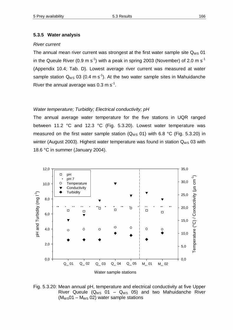
5 Prey availability 5.3 Results 166
5.3.5 Water analysis
River current
The annual mean river current was strongest at the first water sample site QWS 01
in the Queule River (0.9 m s-1) with a peak in spring 2003 (November) of 2.0 m s-1
(Appendix 10.4; Tab. D). Lowest average river current was measured at water
sample station QWS 03 (0.4 m s-1). At the two water sample sites in Mahuidanche
River the annual average was 0.3 m s-1.
Water temperature; Turbidity; Electrical conductivity; pH
The annual average water temperature for the five stations in UQR ranged
between 11.2 °C and 12.3 °C (Fig. 5.3.20). Lowest water temperature was
measured on the first water sample station (QWS 01) with 6.8 °C (Fig. 5.3.20) in
winter (August 2003). Highest water temperature was found in station QWS 03 with
18.6 °C in summer (January 2004).
Water sample stations
pH a
nd T
urbi
dity
(mg
l-1)
0,0
2,0
4,0
6,0
8,0
10,0
12,0
Tem
pera
ture
(°C
) / C
ondu
ctiv
ity (µ
s cm
-1)
0,0
5,0
10,0
15,0
20,0
25,0
30,0
35,0pH pH 7Temperature Conductivity Turbidity
QWS
01 QWS
02 QWS
03 QWS
04 QWS
05 MWS
01 MWS
02
Fig. 5.3.20: Mean annual pH, temperature and electrical conductivity at five Upper
River Queule (QWS 01 – QWS 05) and two Mahuidanche River (MWS01 – MWS 02) water sample stations

5 Prey availability 5.3 Results 167
The annual average water temperatures for the stations MWS 01 and MWS 02 in
Mahuidanche River averaged 11.5 °C to 11.7 °C with a range from 7.0 °C in July
2003 to 17.1 °C in January 2004 (Appendix 10.4; Tab. D).
The annual mean turbidity showed little variation between sample stations and
ranged from 2.5 – 3.5 mg l-1 (Fig. 5.3.20). Highest concentrations were found at
water sample station QWS 04 and MWS 02 with 7.0 mg l-1 in autumn (March 2003)
and in winter (August 2003), respectively (Appendix 10.4; Tab. D).
The pH value in the UQR and Mahuidanche River was always below pH 7.0,
which stands for a temperate basic watercourse (Fig. 5.3.20; Appendix 10.4;
Tab. D).
Electrical conductivity in the UQR was low on average (Fig. 5.3.20). The lowest
annual mean value was measured at the sample station QWS 01 with 15.2 µS cm-1
and the highest value at the fourth station (QWS 04) with 29.4 µS cm-1. However,
the lowest conductivity was measured at station QWS 01 in winter (September) with
6.0 µS cm-1 and highest conductivity was observed at the water sample station
QWS 03 in winter 2003 (August) with 59.0 µS cm-1 (Appendix 10.4; Tab. D). At the
water sample stations MWS 01 and MWS 02 in Mahuidanche River the annual mean
values ranged between 23.3 – 25.8 µS cm-1. The highest value was measured at
station QWS 05 in winter 2003 (July) with 128 µS cm-1. The conductivity in the UQR
steadily increased from the first water sampling station to the fourth
(QWS 01 - QWS 04) and decreased at the fifth station (QWS 05).
Chemical oxygen demand; dissolved oxygen demand
In the Queule River station QWS 01 the lowest annual mean value of chemical
oxygen demand (COD) was measured (6.3 mg l-1) with an increasing trend
towards the fifth water sample station (11.0 mg l-1) (Fig. 5.3.21; Appendix 10.4;
Tab. D). The lowest COD was measured at QWS 02 with 0.5 mg l-1. The first water
sampling station in Mahuidanche River had the lowest annual mean COD value at
5.2 mg l-1, and at the second station the value was 8.8 mg l-1.

5 Prey availability 5.3 Results 168
Water sample stations
mg
l-1
0,0
2,0
4,0
6,0
8,0
10,0
12,0
14,0
16,0
COD DO
QWS
01 QWS
02 QWS
03 QWS
04 QWS
05 MWS
01 MWS
02
Fig. 5.3.21: Mean annual Chemical Oxygen Demand (COD) and Dissolved
Oxygen (DO) at five Upper River Queule (QWS 01 – QWS 05) and two Mahuidanche River (MWS 01 – MWS 02) water sample stations
Both rivers were consistently well oxygenated. The saturation was usually almost
100 % or higher. The annual mean dissolved oxygen (DO) concentration varied
between 11.13 – 11.74 mg l-1. The lowest DO was measured in the summer
(March 2004) at MWS 02 with 7.87 mg l-1 and the highest in the spring (September
2003) 17.73 mg l-1 at station MWS 01 (Fig. 5.3.21; Appendix 10.4; Tab. D).
Nitrate, Nitrite, Ammonia, Norg
The concentration of nitrates, nitrites, ammonia, and organic nitrogen were very
low in general (Fig. 5.3.22; Appendix 10.4; Tab. D). Nitrates levels were higher in
the UQR (53.7 – 85.2 µg l-1) than in the Mahuidanche River (33.8 – 48.6 µg l-1). An
increase of nitrates was monitored downstream of Queule River. The highest
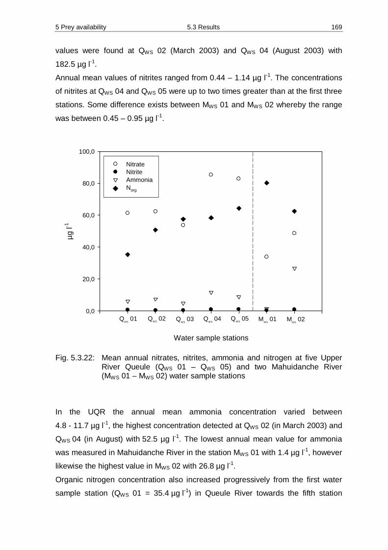
5 Prey availability 5.3 Results 169
values were found at QWS 02 (March 2003) and QWS 04 (August 2003) with
182.5 µg l-1.
Annual mean values of nitrites ranged from 0.44 – 1.14 µg l-1. The concentrations
of nitrites at QWS 04 and QWS 05 were up to two times greater than at the first three
stations. Some difference exists between MWS 01 and MWS 02 whereby the range
was between 0.45 – 0.95 µg l-1.
Water sample stations
µg l-1
0,0
20,0
40,0
60,0
80,0
100,0
NitrateNitriteAmmonia Norg
QWS
01 QWS
02 QWS
03 QWS
04 QWS
05 MWS
01 MWS
02
Fig. 5.3.22: Mean annual nitrates, nitrites, ammonia and nitrogen at five Upper
River Queule (QWS 01 – QWS 05) and two Mahuidanche River (MWS 01 – MWS 02) water sample stations
In the UQR the annual mean ammonia concentration varied between
4.8 - 11.7 µg l-1, the highest concentration detected at QWS 02 (in March 2003) and
QWS 04 (in August) with 52.5 µg l-1. The lowest annual mean value for ammonia
was measured in Mahuidanche River in the station MWS 01 with 1.4 µg l-1, however
likewise the highest value in MWS 02 with 26.8 µg l-1.
Organic nitrogen concentration also increased progressively from the first water
sample station (QWS 01 = 35.4 µg l-1) in Queule River towards the fifth station

5 Prey availability 5.3 Results 170
(QWS 05 = 64.4 µg l-1). However, the highest annual mean organic nitrogen value
was measured in Mahuidanche River (MWS = 80.2 µg l-1).
Sulphate; Phosphate; Silicate
The range of annual mean sulphate concentration found in the Queule River was
1.2 – 3.0 mg l-1. The highest values were measured in QWS 02 and QWS 04 with
11.8 mg in March and August 2003 respectively. The water sample stations in
Mahuidanche River also revealed different values as MWS 01 was lower
(1.3 mg l-1) as MWS 02 (2.5 mg l-1) (Fig. 5.3.23; Appendix 10.4; Tab. D).
Water sample stations
Sul
phat
e / S
ilica
te (m
g l-1
)
0,0
2,0
4,0
6,0
8,0
10,0
Pho
spha
te (µ
g l-1
)
0,0
20,0
40,0
60,0
80,0SulphatePhosphateSilicate
QWS
01 QWS
02 QWS
03 QWS
04 QWS
05 MWS
01 MWS
02
Fig. 5.3.23: Mean annual sulphates, total phosphorous and turbidity at five Upper
River Queule (QWS 01 – QWS 05) and two Mahuidanche River (MWS 01 – MWS 02) water sample stations
Total phosphates varied strongly in between water sampling stations in Queule
River (Fig. 5.3.23; Appendix IV, Tab. D). The lowest annual mean was measured
in QWS 01 (23.9 µg l-1) and the highest in QWS 04 (72.2 µg l-1). Water sampling
station QWS 04 also showed high variation within the year with a peak of
180.1 µl l-1 in autumn (June 2003). Average phosphate values for the
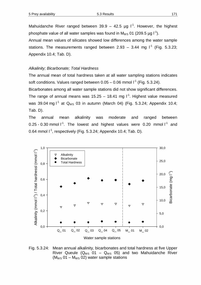
5 Prey availability 5.3 Results 171
Mahuidanche River ranged between 39.9 – 42.5 µg l-1. However, the highest
phosphate value of all water samples was found in MWS 01 (209.5 µg l-1).
Annual mean values of silicates showed low differences among the water sample
stations. The measurements ranged between 2.93 – 3.44 mg l-1 (Fig. 5.3.23;
Appendix 10.4; Tab. D).
Alkalinity; Bicarbonate; Total Hardness
The annual mean of total hardness taken at all water sampling stations indicates
soft conditions. Values ranged between 0.05 – 0.06 mmol l-1 (Fig. 5.3.24).
Bicarbonates among all water sample stations did not show significant differences.
The range of annual means was 15.25 – 18.41 mg l-1. Highest value measured
was 39.04 mg l-1 at QWS 03 in autumn (March 04) (Fig. 5.3.24; Appendix 10.4;
Tab. D).
The annual mean alkalinity was moderate and ranged between
0.25 - 0.30 mmol l-1. The lowest and highest values were 0.20 mmol l-1 and
0.64 mmol l-1, respectively (Fig. 5.3.24; Appendix 10.4; Tab. D).
Water sample stations
Alka
linity
(mm
ol l-1
) / T
otal
har
dnes
sl (m
mol
l-1)
0,0
0,2
0,4
0,6
0,8
1,0
Bica
rbon
ate
(mg
l-1)
0,0
5,0
10,0
15,0
20,0
25,0
30,0
Alkalinity Bicarbonate Total Hardness
QWS
01 QWS
02 QWS
03 QWS
04 QWS
05 MWS
01 MWS
02
Fig. 5.3.24: Mean annual alkalinity, bicarbonates and total hardness at five Upper
River Queule (QWS 01 – QWS 05) and two Mahuidanche River (MWS 01 – MWS 02) water sample stations

5 Prey availability 5.3 Results 172
Chloride; Salinity
In Queule River the annual mean concentrations of chlorides were highest at
water sample station QWS 05 (3.90 mg l-1) (Fig. 5.3.25; Appendix 10.4; Tab. D),
whereas the lowest annual mean concentration was found at QWS 02 (3.05 mg l-1).
In contrast to these findings, chlorides in both water sample stations at
Mahuidanche River had lower values (2.49 – 2.92 mg l-1).
Salinity concentrations varied little among all water sample stations. The range
averaged 0.10 – 0.11 (Fig. 5.3.25; Appendix 10.4; Tab. D).
Water analysis stations
Chl
orid
(mg
l-1)
0,0
1,0
2,0
3,0
4,0
5,0
Sal
inity
0,00
0,05
0,10
0,15
0,20
0,25
0,30
ChloridSalinity
QWS
01 QWS
02 QWS
03 QWS
04 QWS
05 MWS
01 MWS
02
Fig. 5.3.25: Mean annual chlorides and salinity at five Upper River Queule (QWS 01 – QWS 05) and two Mahuidanche River (MWS 01 – MWS 02) water sample stations
5 Prey availability 5.4 Discussion 173
5.4 Discussion
5.4.1 Methodology
Prey availability
Usually long periods of investigation are needed to obtain information about
amphibian richness or density (in scale of years). Short sampling efforts often do
not give total number of species present (SCOTT, 1994), therefore more
quantitative short-term sampling should be performed. In the present study only
nine stations were investigated once, therefore results should be interpreted with
caution.
Two inventory methods were used: 1) patch sampling and 2) straight-line drift
fences with pitfall traps. No amphibians were captured by strait-line drift fences
even near boggy areas. This may due to non-migratory behaviour of the
amphibians at this time and/or to a very restricted spatial defence of their territory.
In contrast the patch sampling technique was more useful. However, by using this
method, personal abilities may have, to a certain degree, influenced the results of
species richness and abundance. Additional, some areas of research interest were
not accessible due to dense vegetation and high water level.
For investigation on the river biocoenosis, two techniques were performed; “red de
palito” and electrofishing. By using the “red de palito” – method bias can result due
to failing to capture biotic material which passed at the side of the net while flipping
up river bed material with feet (pers. obs.). Furthermore problems exist by
investigating bigger objects (e.g. woody debris) as these provide a hiding-place for
crustaceans in higher positions and collecting with “red de palito” was almost
impossible. Therefore the “red de palito” – method is only helpful for crustaceans
in substrate at the river bed level.
Electrofishing was restricted to summer where river sections depth did not exceed
1.20 m and current was low. Consequently samples do not represent the true
species diversity and composition as fish species prefer different habitat
compositions like water depth, current, river bed structure and elevation (e.g.
JOWETT & RICHARDSON, 1996).

5 Prey availability 5.4 Discussion 174
A further bias was the loss of some crustacean legs when electro stunned which is
not considered in biomass calculations and could lead to an underestimate of
biomass.
As the electrofishing technique showed a higher sampling success, in aquatic
species as well as in number of crustacean, in contrast to the “red de palito” –
method, electrofishing forms the main method in the present study for the
investigation of prey availability in the UQR.
Spraint analysis
To investigate the diet of an animal several methods, such as direct observations,
examination of stomach content or faeces analysis, exist (for review see:
JORDAN, 2005). However, the feasibility is dependant upon the species.
Observations in foraging otter species which show diurnal activity and the
examination of stomach content have been successfully used, e.g. Enhydra lutris
(ESTES et al., 1981; ESTES et al., 2003; OSTFELD, 1982), Lutra lutra
(HEGGBERGET, 1995; HEGGBERGET & MOSEID, 1994; KRUUK &
MOORHOUSE, 1990; WATT, 1991), Lontra canadensis (MELQUIST &
HORNOCKER, 1983; TOWEILL, 1974), Lutra maculicollis (STUART, 1981, cited
in LARIVÌERE 2002) and Lontra felina (MEDINA, 1995). However, the southern
river otter is an elusive living animal and observations on feeding or findings of
dead animals for stomach analysis are rare. Therefore the method of faeces
analysis has to be used, which is common and widely used as an indirect method
for otter diet analysis (e.g. CARSS & PARKINSON, 1996; JEDRZEJEWSKA et al.,
2001; KRUUK & MOORHOUSE, 1990; MEDINA-VOGEL et al., 2004; SOMERS &
NEL, 2003).
A confounding component in faeces analysis is that soft parts are digested and
hard parts remain in a distinct condition for examination. This fact makes it difficult
to verify species or to calculate the weight and size of prey eaten by the otter and
may result in an underestimation of soft parts. A further bias is the availability of
faeces, as the animals may defecate into the water too, as it is described for
Lutra lutra (KRUUK, 1995).
CARSS & PARKINSON recommend collecting faecal samples within a few weeks
as they are ephemeral, which is mainly the case in winter, when heavy
5 Prey availability 5.4 Discussion 175
precipitation occurs. In this study it was attempted to collected faeces samples
every month for 14 consecutive days daily to minimize the influence of weather
conditions which may lend to a misinterpretation in the results of seasonal
variations.
Bias resulting from sample size is the main factor affecting the accuracy of faeces
analysis (CARSS & PARKINSON, 1996). For the otter species Lutra lutra, which is
the species with the widest distribution of all otter species, occurring in Europe,
Africa, and Asia (REUTHER & HILTON-TAYLOR, 2004), faecal sample size can
reach up to 1000 within a few month (TAASTRØM & JACOBSON, 1999).
However, for other otter species, like Aonyx capensis (PARKER et al., 2005),
Lontra longicaudis (GORI et al., 2003; WATSON & LANG, 2003), and Lontra
provocax (GONZALEZ LAGOS, 2006; MEDINA, 1998; MEDINA, 1997) a sample
quantity between 60 and 242 were used. In this study marking sites were
resampled to survey seasonal variations for a period of 17 months and 606 faeces
samples were obtained.
Water analysis
Due to laboratory limitations, metal concentrations were not measured in this
study. However, it is important to consider that metals can have a high influence
on organisms as, for example, iron oxides can lower pH (WHITNEY & WRIGHT,
1975) and furthermore iron is known to be responsible for gill-damage and death
of fish (DALZELL & MACFARLANE, 1999; PEURANEN et al., 2002).
There are also indirect influences of metal on fish, which can accumulate metal
through preying on metal burdened aquatic insects and this is also assumed to
have lethal effects on fish (SAIKI et al., 2004).

5 Prey availability 5.4 Discussion 176
5.4.2 Prey availability
The purpose of my investigation is to reach a conclusion about whether the
southern river otter is a high food specialist, or whether it is nourished primarily by
feeding on remaining prey. In order to reach a conclusion, knowledge of the
diversity and abundance of prey species is essential.
5.4.2.1 Diversity and abundance Amphibians
The proportion of the two prominent amphibian species that were collected,
Batrachyla leptopus (55.2 %) and Batrachyla taeniata (44.8 %), was quite similar.
However, the two Batrachyla species differ significantly in length and weight.
Interestingly, more male representatives were found in both Batrachyla species.
BARTELT et al. (2004) attributes the prevalence of males as a sexual difference
in habitat selection. TEIXEIRA et al. (2002) found that gender differences varied
with the seasonal changes that occur throughout the year.
Amphibian abundance was strongly influenced by the presence of marsh grass
Juncetum procerii and by the abundance of leaf litter (Fig. 5.3.3; p. 140) found
near areas where there are small runlets of water. MÉNDEZ-TORRES et al.
(2005), while conducting an inventory in the X. Region of Chile, found amphibian
abundance in a variety of microhabitats. Such microhabitats include those where
moss is present, and areas under tree trunks, under stones and in runlets. The
geographical location for my study on prey availability of amphibian, however, did
not include the same microhabitats found in X. Region of Chile. In the present
study, habitats such as those described by MÉNDEZ-TORRES et al. (2005) were
absent, or were only found in small numbers in this predominantly anthropogenic
influenced study area. As this area is widely used for livestock farming and
forestry, suitable and attractive habitat structures for amphibians are rare.
Furthermore, several studies have shown that amphibian abundance declines
when the natural habitat is negatively impacted, or when anthropogenic influences
modify pasture land and roads, and cause deforestation of the woodlands (e.g.
KOLOZSVARY & SWIHART, 1999; TEIXEIRA et al., 2002; TODD &
ROTHERMEL, 2006). Stream amphibians, in particular, may be negatively
influenced by clear cutting in the study area as a result of fine sediments from

5 Prey availability 5.4 Discussion 177
erosion that can stay in the headwaters for several decades creating a
transformed habitat that is unsuitable.
Two species, Caudiverbera caudiverbera and Pleurodema thaul were
unexpectedly detected in study areas that were close to marsh grass. These
species were not known to live in these study areas. It appears that during
previous inventory studies, conducted by other scientists, C. caudiverbera and
P. thaul had not been collected; therefore, it is evident that sampling methods
may play an important role in obtaining accurate data. Sampling methods may
result in the collection of only some of the species living in the habitat being
studied.
A contributing factor that may influence the appearance and abundance of
amphibians is the use of pesticides by the forestry industry in their attempts to
control pest invasion. Insecticides and herbicides can reach surface water through
runoff from treated plants or soil, or by aerial overspray (THOMPSON et al.,
2004). Practices such as these have an indirect and/or direct effect on the
biodiversity and productivity of aquatic communities (RELYEA et al., 2005;
RELYEA, 2005a). Roundup®, an herbicide, was used in pine and eucalyptus
plantations along the UQR. Detailed studies on Roundup® and its impact on the
aquatic and terrestrial amphibians by RELYEA (2005b) show that 96-100 % of
larval amphibians were killed after three weeks; and, it caused high lethal impact
rates on juvenile amphibians. Therefore, the lack of abundance of amphibians in
this area may not only be a result of fragmentation and habitat destruction, but
also a consequence due to the utilization of the herbicide Roundup® commonly
used over the past several years in forest plantations in the study area.
Fish and crustaceans
Twelve crustacean species are described by JARA et al. (2006) for the IX. Region.
The same region where this study was conducted. However, in this study, a total
of only two malacostracan species were detected in different sections of Queule
and Mahuidanche River. The method used for crustacean trapping may not be
effective enough to collect all species that are actually present in the water. If the
method was not sufficiently effective, low diversity would have resulted.
S. spinifrons, for example, is a species which hides itself under or in river bed

5 Prey availability 5.4 Discussion 178
structures. As a contrast, Parastacus spec. also occurs in the IX. Region (JARA et
al., 2006); however, it is a burrowing species that can be encountered in horizontal
tubes in riparian walls (pers. comm., JARA). Therefore, it may be true that
Parastacus spec. do not exist in the shallow waters where electro fishing was
performed as part of this study. There was no evidence, however, of other
crustacean species that might serve as important food sources for the otter. In
addition, no other crustacean remains were detected in otter faeces.
While the ichthyofauna of Chile is characterized as being of low diversity, it is
known to be of high endemism (HABIT & VICTORIANO, 2005). This study
supports their findings. Six out of the thirty-nine known native freshwater species
of Chile (DYER, 2000) and two introduced species where found in the investigated
area (Tab.5.3.2, page 143). The study area was not found to have richly diverse
populations. On average, three species were found per investigation site;
therefore, the density of species found in the study area was very low compared to
numbers found in other studies conducted on continental rivers. TAYLOR (1969,
cited in: JOWETT & RICHARDSON 1996) examined more than 82 species in a
tributary of the Mississippi. However, the average species richness is similar to
findings of JOWETT & RICHARDSON (1996) in New Zealand where, on average
three to five species were collected per investigation site and may be transferable
to Chile freshwater systems.
Influencing factors
Fish and crustacean diversity, abundance, as well as biomass are influenced by a
multitude of factors. One of the more influential factors is that of the riverbed
structure because it must provide a suitable habitat where aquatic organisms can
spawn, grow, acquire food, and protect themselves from predators.
The most common substrate type encountered by aquatic animals in the UQR is
sand (Appendix 10.4; Tab. C). Additionally, aquatic organisms encounter a lower
abundance of gravel and woody debris. According to local inhabitants, these
substrates were absent in this area 10 – 20 years ago. Sediment input rose as a
result of clear cutting by the forestry industry, resulting in serious land (soil)
erosion (e.g. GOMI et al., 2004). According to GRANT & WOLFF (1991) sediment

5 Prey availability 5.4 Discussion 179
in the river can increase up to twelve times, and may stay for more than 10 years,
as a result of timber harvesting. Siltation negatively impacts fish species
(CASATTI et al., 2006) and may be responsible for low diversity in the UQR. On
the other hand, some species may benefit from the change. For example, in this
study, juvenile Geotria australis were the predominant species collected.
Geotria australis burrow into fine sediment where they undergo metamorphoses
from the larval stages to the adult phase (BEAMISH & JEBBINK, 1994;
HARDISTY & POTTER, 1971; KELLY & KING, 2001). The most common substrate typically found in a rithral zone is gravel
(SCHWOERBEL, 1994), however, in this study, it was only second most
commonly found substrate. The crustacean species, A. abtao, was identified in
this study to have a preference for rocky habitats. This is supported by the
research done by SCHMITT (1942). Furthermore the fish species
Trichomycterus areolatus, was found in the study area as well, is a species also
adapted to rithral habitats (HABIT et al., 2005).
The highest species diversity in the UQR was found to exist in substrates where
there was an abundance of woody debris. This is similar to the research done by
WRIGHT & FLECKER (2004) where a higher diversity of fish species were found
in pools that contained woody debris. ANGERMEIER & KARR (1984) assumed
that association between fish diversity and woody debris is more related to
protecting fish from predation than an association based on increased food
availability. This assumption was supported by EVERETT & RUIZ (1993) in their
experimental conclusions for epibenthic fish and for invertebrates. In addition to
the fact that woody debris provides shelter for aquatic animals, thereby
decreasing predation risk, it also offers visual isolation and water velocity refuge
(CROOK & ROBERTSON, 1999). These findings may also be transferable to
S. spinifrons and A. abtao the most abundant species found in this type of
substrate. Since woody debris is also colonized by other invertebrates (BENKE,
1998), it may, however, also serve as a food source for crustaceans.
In contrast to the findings of AGERMEIER & KARR (1984), in this study only
smaller-sized fish, namely, Cheirodon galusdai, Percichthys trucha,
Salmo trutta fario, inhabited the waters where woody debris was found. It is
assumed that these three species used the woody debris for protection from
predators, since other structures such as roots and aquatic plants were limited in

5 Prey availability 5.4 Discussion 180
number or were non-existent. In general, it seems that woody debris is an
important structural element for aquatic animals. Another important fact is that
small to medium-sized woody debris, as well as large-sized woody debris seems
to be important. The variety of sizes of woody debris causes a high geomorphic
impact on the river structure (e.g. KAIL, 2005) by building dam pools, plunges and
backwater scours (DOLLOFF, 1994), where smaller woody debris accumulates,
thus creating a preferable habitat for fish and macroinvertebrates
(HILDERBRAND et al., 1997; LEMLY & HILDERBRAND, 2000; NAKAMOTO,
1998).
The comparative section of the Mahuidanche River contains aquatic plants that
are not present in UQR and has a species community that is different
(see Fig. 5.3.5, p. 144; Fig. 5.3.6, p. 145). These findings are similar to the results
of several authors (e.g. CHARÁ et al., 2006; LAMOUROUX et al., 1999; VLACH
et al., 2005) where each fish species prefers specific habitat structures. In
contrast to the UQR, where both crustacean species, S. spinifrons and A. abtao,
are the most abundant stock-forming species, the fish species Galaxias
maculates is eudominant (see Fig. 5.3.9; p. 148) suggesting it may have chosen
the aquatic plants as a breeding habitat since only small fishes were caught.
JOWETT & RICHARDSON (1995) suggested that water depth is more important
than riverbed structure in determining species composition; species composition
varies considerably with water depth. It is important to note that, in this study,
examination of river depth was not applicable because electrofishing was
conducted in rivers only at depths that were < 1.4 m. Furthermore, there remains
the question of whether elevation is an influencing factor for species composition,
as was shown by JOWETT & RICHARDSON (1996) in New Zealand.
Nevertheless, the aim of the study was not to detect differences in krenal, rhitral
and potamal zones, but to find differences within a river length of 20 km where
faecal samples of southern river otters were able to be collected.
MERRINER et al. (1976) described that seasonal migration of fishes has an effect
on the abundance and species diversity of fishes in lotic habitats. This was not
considered in this study since electrofishing was done only in the summer when
river water levels were low. Furthermore, the low diversity and abundance of
fishes may be explained as being the result of high crustacean abundance, as
both feed on the same macroinvertebrates (HANSON et al., 1990). On the other

5 Prey availability 5.4 Discussion 181
hand, Samastacus spec. and Aegla spec. are also known to be prey for
Salmo trutta fario and Oncorhynchus mykiss (SOTO et al., 2006), and both
species were found to occur in the UQR.
The resulting biomass of the examined river is not only a factor of abundance, but
is influenced by the age and size of the aquatic animals. Therefore, fish biomass
is low in the UQR (see Fig. 5.3.11 a; p. 150) as a result of the fact that only
juveniles of Salmo trutta fario were collected in investigated sites. In contrast to
the Mahuidanche River, the resulting fish biomass depended not only on the high
abundance of Galaxias maculates, but on weight of adult Oncorhynchus mykiss
and Salmo trutta fario as well.
Both species, Oncorhynchus mykiss and Salmo trutta fario are introduced fish
species which show a widespread occurrence and are often a result of
management for sport fishery and aquaculture in Chile (CAMPOS & MORENO,
1985; PÉREZ-LOSADA et al., 2002; SOTO et al., 2006). It is presumed by
several authors (e.g. ADAMS et al., 2001; SOTO et al., 2006) that they have an
indirect impact on native species since they place a predatory pressure on them.
MCDOWELL (2003) points out that in New Zealand, which is considered the
closest comparison for introduced fish species, Oncorhynchus and Salmo trutta
seem to harm the native fish fauna. For example native fish and introduced brown
trout were never found in the same section of a river (TOWNSEND & CROWL,
1991; cited in: SOTO, D. et al. 2006 ).
ARENA (1978) observed that predation on native fish by Oncorhynchus mykiss
was only observed when the species sizes were larger than 30 cm. The introduced
fish species in UQR, however, were much smaller than 30 cm.
In line with the study of SOTO et al. (2006), where introduced fish constitutes the
highest abundance and main biomass in river and lakes in Chile, are the findings
of the present study. However, as this study also considers that crustacean
species serve as a vital source of prey for the southern river otter, they form the
main biomass in the UQR (see Fig. 5.3.11; p. 150).
The biomass calculated in 2003 showed a significant difference to 2004
(see Tab. 5.3.3; p. 154), which is assumed to be as a result of the previous
flooding in 2004. In contrast to THEILING et al. (1999), the river sections did not

5 Prey availability 5.4 Discussion 182
immediately show a recruitment neither an increase of native fish diversity.
However, electrofishing was not done directly before the flooding and species
diversity, abundance and biomass may have already changed compared to 2003.
Nevertheless, I presume that flooding would form new habitat structures as large
amounts of woody debris and areas of gravel and stones disappeared in several
sections and newer woody debris emerged which had to be recolonised by fish
and crustaceans. All fish species showed a decrease in abundance after flooding,
except for Salmo trutta fario. This is consistent with ORTLEPP & MÜRLE (2003)
where fish abundance of Salmo trutta fario was not reduced by an experimental
flooding and supports the findings of TEW et al. (2002), who report that species
were affected differently by the impact of a typhoon in a mountain stream in
Taiwan. Furthermore TEW et al. (2002) show that species abundance did not
recover immediately but took a period of 14 to 17 months.
In addition to the previous factors, water quality is also important as it can
influence prey species diversity and abundance (REASH & PIGG, 1990) and
therefore will have an impact on the habitat suitability for the otter. Not all
parameters which were measured may be important for the assessment of the
river as an otter habitat, but they provide a comprehensive insight into the
physico-chemical situation for the UQR and can be used for comparison for
further studies on other rivers.
In general, the water of the UQR is characterized by its low hardness and low
conductivity, but high oxygen concentration. The pH is on average slightly acid,
which may be normal in rivers without carbonate rocks such as limestone and
dolomite, whereby the very low alkalinity results, which stands for the low
buffering possibility of the water. However, the pH values are still in the
appropriate range for normal development of freshwater fish (EIFAC, 1969).
The measured temperatures show the typical fluctuations regarding the seasons
which are typical for the rithral, where the maximum temperature does not exceed
20 °C (SCHWOERBEL, 1994).
Typical environmental pollution parameters are correlated to villages which
discharge their waste water directly into the river, being higher in these areas
compared to undisturbed areas. Thus station QWS 04 and QWS 05 show higher
values in chloride, phosphate, sulphate, nitrate, Norg, ammonia, conductivity and

5 Prey availability 5.4 Discussion 183
turbidity as well as in chemical oxygen demand. However, high variations were
also demonstrated for the other station throughout the year and may result from
the varying use of a forest camp site by lumber men and the school during the
year, where waste water is also discharged directly into the river.
The two sites in Mahuidanche River, which were measured for comparison
showed similar values compared to the Queule River. However, site MWS 02 is
situated close to pasture land with stock farming and has a seasonal very low
water current. Animal excrements may discharge into the water section MWS 02
and therefore values of nitrogen compound, phosphate and chemical oxidant
demand were in general higher than for station MWS 01.
All measured physico-chemical parameters showed values below that required for
critical or toxic effects on fish (SVOBODOVÁ & VYKUSOVÁ, 1991) and may also
not be critical for crustaceans. However, through the very low buffer possibility,
this lotic habitat is interference sensitive to any changes and an increase of
H - concentration could threaten the egg and larvae development of fish (e.g.
PETERSON et al., 1981; WHITNEY & WRIGHT, 1975) and crustaceans
respectively.
5.4.3 Diet composition The most reliable estimation of prey in faeces is given by weight or volume,
although frequency of occurrence (either as percentage or relative frequency)
provides at least an accurate rank order of prey classes (CARSS & PARKINSON,
1996; JACOBSEN & HANSEN, 1996; WISE et al., 1981). Frequency of
occurrence is the most commonly used method and provides data for comparison
to previous work on diet analysis on otters. However, inaccuracies in faecal
analysis still exist.
Malacostracan, in particular S. spinifrons dominated the diet of the southern river
otter in the study area (see Tab. 5.3.5; p. 156). These findings are consistent with
previous studies on southern river otter diet in freshwater habitat in several
publications (e.g. CHEHÉBAR et al., 1986; GONZALEZ LAGOS, 2006; MEDINA-
VOGEL et al., 2003). The abundance of S. spinifrons in the diet of L. provocax is
5 Prey availability 5.4 Discussion 184
consistent with the results of prey availability where S. spinifrons is the most
dominant aquatic prey species in the UQR. Similar to the findings of MEDINA-
VOGEL et al. (2003), which were conducted in a nearby area of the Queule River,
is the poor abundance of A. abtao. A higher abundance of Aegla spec. is
registered in lakes and Andean rivers, where Aegla spec. is also more abundant in
southern river otter diet (CHEHÉBAR, 1985; MEDINA, 1997; MEDINA, 1998). The
habitat in the Andean region for A. abtao may not be influenced by increased
sedimentation in the river by deforestation, like it occurs in the mountain range,
and therefore the preferred rocky aquatic habitat of A. abtao is not diminished.
Similar to previous studies on the diet of L. provocax fish form a minor part of otter
faeces (e.g. CHEHÉBAR et al., 1986; GONZALEZ LAGOS, 2006; MEDINA-
VOGEL et al., 2003). In contrast to the findings of prey availability, three species of
fish, C. galusdai, G. australis and T. areolatus, were not discovered in faeces.
Usually operculum, vertebrae and scales are used for fish determination
(FELTHAM & MARQUISS, 1989; HAJKOVA et al., 2003; JENKINS & HARPER,
1980; MIRANDA et al., 2005; WISE et al., 1981), however, these key items were
mostly absent which resulted in only three fish species being determined, a high
frequency of undeterminable fish species and no categorization of fish size.
Surprisingly, scales were almost never detectable; even though other remains of
fish were present.
Lutra lutra starts to consume the fish from head (ERLINGE, 1968; RUIZ-OLMO et
al., 1998), which may be serve to kill the prey rapidly, and consequently, remains
for fish determination are absorbed. RUIZ-OLMO (1998) noted that fish with less
than 100g were eaten completely. However when larger fish are captured by
L. lutra, no starting priority seems to exist, it has been observed to start from the
side or tail of the fish and may leave the head (CARSS et al., 1990; KRUUK &
MOORHOUSE, 1990; RUIZ-OLMO et al., 1998). This is contrary to observations
on housed L. provocax (Chapter 2), where provided fish was always eaten from
tail as the starting point and head was consistently left, independent of size of
provided fish and important parts for fish determination were thereby excluded.
Nevertheless it has to be taken into consideration that this observation of fish
feeding was done in captivity and L. provocax was fed with dead fish. No
behavioural observation of fish consumption on free ranging L. provocax exists
and no remains of fish or crustacean on land were left by L. provocax as it is

5 Prey availability 5.4 Discussion 185
known for L. lutra (RUIZ-OLMO et al., 1998). On several occasions L. provocax
was observed feeding on crustaceans. At the time of consumption the southern
river otter always stayed in the river and consumed the crustacean entirely on the
water surface.
Diet composition on L. provocax is similar to A. capensis (Cape clawless otter)
where crustacean also dominate the diet in freshwater habitats (PARKER et al.,
2005; PERRIN & CARUGATI, 2000; ROWE-ROWE & SOMERS, 1998). In
contrast, fish was relatively unimportant for A. capensis but amphibians were
second most prevalent in the diet. The importance of amphibians as a staple prey
is also known for L. lutra in northern Europe, especially in river habitats
(BRZEZINSKI et al., 1993; CLAVERO et al., 2005; JEDRZEJEWSKA et al., 2001;
LANSZKI et al., 2006; SULKAVA, 1996). The abundance of amphibians in otter
diet was higher when their availability increased (JEDRZEJEWSKA et al., 2001).
Amphibians as prey for L. provocax were not detected in this study, which may be
due to the absence of good amphibian habitats and resultant low abundance.
However, L. provocax is also known to prey on amphibians, but these seem to
have a minor importance as they only occur in faecal samples in small numbers
(GONZALEZ LAGOS, 2006; MEDINA, 1997; MEDINA-VOGEL et al., 2003).
On four occasions the remains of the bivalve Diplodon chilensis is recorded in the
otter faeces. This common occurring mussel in southern Chilean rivers (PARADA
& PEREDO, 2002) may be taken as a secondary food source or accidentally as it
is found in only small numbers which is consistent with the findings of MEDINA
(1997). However the importance of freshwater mussels may be underestimated as
they comprise more soft parts compared to other prey species. It is unknown if
L. provocax has the ability to open and only feed on the inner part of the mussel.
On some occasions piles of shells on small river islands of D. chilensis were found
but the shells were not damaged. Since L. provocax feed on crustaceans complete
with exoskeleton, shells of mussels should not be a problem as they are relatively
soft. Lontra provocax did not feed on D. chilensis when it was provided to the
caged animals during the trapping season for telemetry.
There was no evidence of predation noted on mammals, frogs, birds and insects
during this study as it is known for several other otter species like L. lutra,
L. canadensis, A. capensis (e.g. CARSS, 1995; MELQUIST & HORNOCKER,

5 Prey availability 5.4 Discussion 186
1983; PARKER et al., 2005) and also described in previous studies for L. provocax
(GONZALEZ LAGOS, 2006; MEDINA, 1998). However it has to be considered that
a lack of appearance in faecal samples does not necessarily represent a lack of
consumption (KRUUK & MOORHOUSE, 1990) as it is possible that the otters may
generally defecate in water (JACOBSEN & HANSEN, 1996; KRUUK et al., 1986;
KRUUK, 1995) and therefore information on southern river otter prey may be
inaccurate. Furthermore the prey availability has to be considered otherwise it is
not possible to draw any conclusions as to whether the investigated animal is a
food specialist/generalist or compelled to nourish on the only available prey.
Southern river otter deaths from car accidents are not reported as they are for
L. lutra in Europe (e.g. HAUER et al., 2002) and findings of carcasses by chance
are seldom. Therefore is a significant diet analysis for L. provocax out of stomach
content not practicable. The two dead southern river otters analysed do not
provide additional information, as only the crustacean species S. spinifrons was
detected in stomach and intestines.
JEDRZEJEWSKA et al. (2001) show that the habitat where the studied otter lives
influences the diet composition. Thus European otters living in a seashore
environment show a strong fish based diet composition which decreases and
becomes more variable for otters living in inland waters. In some crayfish-rich
habitats crayfish was the dominant diet throughout the year for L. lutra
(JEDRZEJEWSKA et al., 2001). These results may also be transferable to
L. provocax as southern river otters which are living in shore areas also prey
predominantly on fish (SIELFELD, 1983) and seems to switch to crustaceans in
freshwater habitats (CHEHÉBAR et al., 1986; GONZALEZ LAGOS, 2006;
MEDINA, 1997; MEDINA-VOGEL et al., 2003). Based on these results it is likely
that L. provocax is not specialist on crustacean, but on prey species abundance.
However, in this study L. provocax is dependant upon the crustacean prey species
being S. spinifrons as the prey diversity and abundance of other aquatic species
was low in the area of investigation.

5 Prey availability 5.4 Discussion 187
5.4.4 Seasonality
Marking frequency
The findings of low faecal samples in the summer season of 2003 when
precipitation was low is consistent with several authors (MASON & MCDONALD,
1986; TAASTRØM & JACOBSON, 1999). However, the results are contrary to
GONZALES LAGOS (2006) who studied faecal samples of L. provocax in a
wetland system. His findings could be caused by low revisiting rate and heavy
rainfall which washed faecal samples away between surveys. Nonetheless, it has
to be considered that the number of faecal samples found between seasons of
high and low precipitations do not differ significantly in this study and the number of
faecal samples in 2004 were almost the same between seasons and incomplete.
Several authors have stated that the variation in the number of faecal samples can
be attributed to manifold factors (e.g. KRUUK, 1992; PRENDA &
GRANDADOLORENCIO, 1996). They have suggested that sprainting rates are
based on prey availability and biomass, but also may depend upon the number of
individuals which occupy a certain area (COPP & ROCHE, 2003; HUTCHINGS &
WHITE, 2000; TAASTRØM & JACOBSON, 1999).
Contrary findings about intersexual marking frequencies exist. Thus argues
CARSS (1995) that male otters mark more frequently with smaller faeces size as
female otter do, whereas KRUUK (1992) did not find significant differences
between the sexes. It has to be considered, that the time range of the present
study may not be sufficient to draw conclusions about factors which influence
marking frequencies.
Diet variation
Seasonal diet variation is influenced by multifaceted factors such as prey
availability (ROWE-ROWE & SOMERS, 1998), activity of prey (KRUUK, 1995),
local abundance (LANSZKI et al., 2006) and ability to catch the prey (ERLINGE,
1968). For example LANZKI et al. (2006) notes that L. lutra consumes European
pond turtles Emys orbicularis when access to fish is low during winter. Likewise the
predation on amphibians increases in winter when they hibernate in river beds, and
during breeding season in spring when they are more abundant (JEDRZEJEWSKA
et al., 2001; SULKAVA, 1996). Introduced species are reported to influence prey
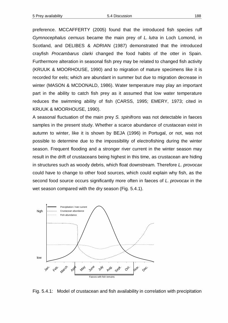
5 Prey availability 5.4 Discussion 188
preference. MCCAFFERTY (2005) found that the introduced fish species ruff
Gymnocephalus cernuus became the main prey of L. lutra in Loch Lomond, in
Scotland, and DELIBES & ADRIAN (1987) demonstrated that the introduced
crayfish Procambarus clarki changed the food habits of the otter in Spain.
Furthermore alteration in seasonal fish prey may be related to changed fish activity
(KRUUK & MOORHOUSE, 1990) and to migration of mature specimens like it is
recorded for eels; which are abundant in summer but due to migration decrease in
winter (MASON & MCDONALD, 1986). Water temperature may play an important
part in the ability to catch fish prey as it assumed that low water temperature
reduces the swimming ability of fish (CARSS, 1995; EMERY, 1973; cited in
KRUUK & MOORHOUSE, 1990).
A seasonal fluctuation of the main prey S. spinifrons was not detectable in faeces
samples in the present study. Whether a scarce abundance of crustacean exist in
autumn to winter, like it is shown by BEJA (1996) in Portugal, or not, was not
possible to determine due to the impossibility of electrofishing during the winter
season. Frequent flooding and a stronger river current in the winter season may
result in the drift of crustaceans being highest in this time, as crustacean are hiding
in structures such as woody debris, which float downstream. Therefore L. provocax
could have to change to other food sources, which could explain why fish, as the
second food source occurs significantly more often in faeces of L. provocax in the
wet season compared with the dry season (Fig. 5.4.1).
Jan.
Feb.
March
April
MayJu
ne July
Aug.
Sept.
Oct. Nov.
Dec.
high
low
Fig. 5.4.1: Model of crustacean and fish availability in correlation with precipitation
Precipitation / river current
Crustacean abundance
Fish abundance
Faeces with fish remains

5 Prey availability 5.4 Discussion 189
The results are similar to ROWE-ROWE (1977) where A. capensis, which feeds
mainly on crustaceans, also consumes more fish during winter than in summer
(PERRIN & CARUGATI, 2000). However, this is contrary to the findings of previous
studies on seasonal variation in the southern river otter diet, where a higher fish
occurrence is noted in dry seasons (GONZALEZ LAGOS, 2006; MEDINA, 1998).
As mentioned before, a low revisiting frequency of marking spots by previous
studies may lead to different results. The food-limitation hypothesis, which predicts that the consumption of sub-optimal
food and the resulting mortality would be highest during the season with low prey
availability, may not be supported in this study, as L. provocax seems to prey on
fish which has higher food quality concerning the kcal content (Appendix 10.4;
Tab. E).
5.4.5 Required quantity of staple prey
Calculation of consumed biomass from faecal samples is questioned by several
authors (RUIZ-OLMO et al., 1998) as some parts of prey may be left by the animal.
In this study not the consumed biomass was calculated, but rather the numbers of
crustaceans a southern river otter needs for its daily metabolic requirement by
measuring the size and quantity of prey found in the faecal samples.
The daily energy requirement of an active southern river otter is not known and the
calculated results are based on caged animals which had a very limited possibility
of movement (see chapter 3). Therefore it is assumed that the metabolic
requirements in free-ranging southern river otters are much higher and
consequently they have an increased prey requirement. However the results of the
present study give the first general survey of energy requirements of southern river
otters.
The factor of digestibility of crustaceans was not considered in the calculation.
BEJA (1996) calculated this to be 0.5 but this factor seems to be related to felines.
Conversely MÅRTENSSON (1994) noted an 81 % - 83 % of digestibility efficiency
of crustacean species by harp seals. Digestibility factors which are calculated for
different species may not be transferable as digestive processes of predators may
have evolved to be more efficient with their main prey (JACKSON et al., 1987). For
example A. capensis shows an adaptation of molariform teeth related to

5 Prey availability 5.4 Discussion 190
geographical variation in their main prey and the size of molluscs and crustaceans
(DAVIS, 1978; cited in LARIVIÈRE, 2001).
The time a southern river otter would need in order to obtain sufficient food can not
be answered, as data of capture rates do not exist and the observation of
L. provocax is very difficult. RUIZ-OLMO (1998) describes that L. lutra needs
2-3 hours of fishing daily to obtain sufficient food, assuming that an otter needs
12-15 % of its corporal biomass as noted by KRUUK (1995). The average time
taken for movement behaviour, which includes travelling, hunting and marking, is
6:30 h as measured by the radio tracking of three southern river otters (Chapter 3).
Usually otters have to increase foraging time when the availability of food
decreases, which usually occurs in winter, in order to meet metabolic requirements
(KRUUK, 1995). This implies that southern river otters should use less time for
foraging in the spring-summer season, however this still has to be proven, as in
this study the radio-tracking took place in the autumn-winter season.
The majority of S. spinifrons that was caught by electrofishing weighed less than
the average individual found in faecal samples of L. provocax, which is the same
for A. abtao. Consequently the following conclusions could be drawn: that in order
to obtain sufficient food: 1) Lontra provocax has to hunt in several different areas
on crustaceans, and/or 2) other food sources, which were not detected in faecal
samples, play an important role.
While radio tracking southern river otters, it was noted that foraging took place in
several home range sections. The kind of prey which was consumed can only be
suggested, as sometimes the typical crushing noise by feeding on crustacean was
noted. However, I assume that L. provocax is foraging regularly on fish to optimize
his metabolic requirements, as fish also has higher food quality in contrast to
crustaceans; as reported by KRUUK (1995); and additionally provides more kcal
per consumed prey unit. A further assumption is that faeces which contain fish
remains are usually not used for marking as they are fluid, highly ephemeral and
therefore are defecated into the water. This assumption is based on observations
on caged animals, where only fish was provided to L. provocax which resulted in
fluid faeces. This is similar to the findings in the field, where only faeces of
crustacean remains consistently showed a compact cylindrical structure. However,

5 Prey availability 5.4 Discussion 191
to maintain markings in the rainy season, when most faeces are flushed away in a
relatively short time, all types of faeces may be used.
5.4.6 Diet – mink versus otter
The diet of the American mink in the UQR (rodents and crustacean) was similar to
the findings of MEDINA (1997) in Chile. Preying of mink on rodents and
crustaceans, revealed in UQR, was reported from other regions as well and
wherever crustaceans were abundant they constituted an important part of the diet
(e.g. BRZEZINSKI & ZUROWSKI, 1992; GERELL, 1967; JEDRZEJEWSKA et al.,
2001; RACEY & EULER, 1983).
The American mink is a generalist predator and known to exploit prey on land as
well as in water habitats where its diet includes mammals, fish, amphibians, birds
and crustaceans (JEDRZEJEWSKA et al., 2001). In this study the absence of fish
in mink faecal samples is noteworthy as consumption of fish can vary between the
seasons but was always present in other diet studies (e.g. FERRERAS &
MACDONALD, 1999; GERELL, 1967; HAMMERSHOJ et al., 2004; WISE et al.,
1981). As the proportion of prey in the mink diet increases with prey abundance
(JEDRZEJEWSKA et al., 2001), it may be concluded that the UQR has a very low
fish abundance, or that the mink has changed its diet because of high otter density
(BONESI et al., 2004) to avoid conflicts with the southern river otter in this area. In
contrast to the otter, the American mink cannot dive and swim for a long time
(DUNSTONE, 1979, in BONESI et al. 2004) and this may also influence its
success in catching fish.
PERSSON (1985) argues that the competition highly favours the European otter,
as its body ratio is 7:1 (weight) compared with the mink, and this would be higher
for southern river otters as they are in average heavier than the European otter.
Furthermore SCHRÖPFER & PALIOCHA (1989) assume that a coexistence of the
European otter and American mink should be possible by applying the
Hutchinson-rule, due to the significant body size difference, competition may
therefore be improbable. This suggestion may be transferable to the southern river
otter as the American mink is the only other semi-aquatic mammal which occurs on
the ecotone bank in the study area. Both species seems to present the guild of
megacarnivorous in the study area.

5 Prey availability 5.4 Discussion 192
However, food competition may be seasonal, as REUTHER (1993) reports
regarding food competition occurring between the American mink and the
European otter in winter, when prey availability is lower. However the low faecal
sample size of M. vison in this study makes examination of seasonal variation
difficult.
Furthermore the results of this study are supported by the assumption of MEDINA
(1997) that no food competition exists between L. provocax and M. vison, as the
Renkonen Index for similar food resources is relatively low. However a low
abundance of mink is suggested by the poor number of faecal samples and this
may be a further reason for no findings of food competition. The situation of food
composition may change with higher mink density.
5 Prey availability 5.5 Prospects 193
5.5 Prospects
In the present study it is assumed that L. provocax depends upon the crustacean
prey species S. spinifrons, because of the low prey diversity and abundance of
other aquatic species in the study area.
However, whether the southern river otter is a food specialist and consumes
primarily crustaceans, or a generalist which consumes the most abundant prey
species still has to be proven. Further research could be done in areas where
abundance of crustaceans are low and in areas where fish, fish farming or ponds
with a year-round fish stocking exist which could provide sufficient food for
L. provocax.
The results of calculations regarding quantities of crustaceans needed for
metabolic requirements are based on caged animals with limited possibility of
movement and provide new basic information. For further studies on energy
requirements and digestibility of several prey items, animals should be kept in big
enclosures in which they are able to swim.

6 Age determination 6.2 Methods 194
6 Age determination of male southern river otter Lontra provocax (THOMAS 1908)
Abstract
Four male skulls of the southern river otter L. provocax were examined for age
determination. Tooth wear; tooth abrasions, dental pulp; relative width of dental
pulp, incremental cementum lines; number of lines, and sutures of the skull; visible
sutures, were used for age determination. By using the methods tooth wear,
incremental cementum lines and relative width of dental pulp it was possible to
classify the animals as juvenile (n=1), subadult-adult (n=1) and senior (n=2).
However, as only the juvenile showed sutures, it was not possible to distinguish
between subadult – adult to senior and therefore sutures on skulls provide
information about age, but have to be used in combination with the other
presented methods for more accurate classification.
6.1 Introduction
Until today the otter species Lontra provocax has been hardly studied. This is due
to the cryptic behaviour of the species, the difficulty of trapping and its population
declination as a result of its vanishing habitat (MEDINA-VOGEL, 1996).
First home range and spacing pattern studies have been conducted only recently.
However, scarce information is available on the demography of L. provocax which
is crucially needed for conservation and wildlife management (ALEXANDER,
1958; MEDINA-VOGEL, 1996; VAN HORN et al., 2003).
Age estimation is an important tool for obtaining information about the
demography of a species (e.g. longevity, mortality) and to monitor population
dynamics (SPINAGE, 1973). Different techniques for age estimation such as
changes of cranial proportion and sutures, eye lens mass, tooth wear, baculum
weight, ossification, coat colour etc., have been used on several carnivores
(ANSORGE, 1995; CATLING et al., 1991; GEIGER et al., 1977; KRÜGER, 1995;
LAWS, 1952). Nevertheless, methods of age determination can be often subject to
error (FIERO & VERTS, 1986); e.g. according to ANSORGE & STUBBE (1995)
the age estimation for Eurasian otters Lutra lutra by tooth abrasion is not even
6 Age determination 6.2 Methods 195
suitable for rough age classification. Therefore multiple methods have to be
compared and verified.
In our preliminary study of feasibility in age estimation we used four different
methods: Tooth wear, dental pulp, incremental cementum lines and sutures of the
skull.
6.2 Methods
A total of four male otter skulls were obtained for age determination from the
Museum of Ecology and Evolution, University Austral of Chile, Valdivia (Museo del
Instituto de Ecología y Evolución de la Universidad Austral de Chile, Valdivia,
Chile). All skulls were collected during 2000 – 2004 when studies on home range
and behaviour patterns were conducted and were provided by the.
As no data is available for the southern river otter tooth wear, only a rough
estimate in age classes was performed. Tooth wear was separated in three age
classes according to KRÜGER (1995) by considering the degree of abrasion:
1. Age class: no abrasion visible (juveniles to subadults).
2. Age class: small to medium abrasion (younger adults to grown adults).
3. Age class: heavy abrasion (seniors).
For examination of the dental pulp the right upper canine was extracted from its
alveolus with dentist forceps without damage from four prepared otter skulls,
stored and labelled in glass vials until further preparation. Due to their size canine
teeth are usually preferred for dental pulp (Pulpa dentis) width measurements in
carnivores (KRÜGER, 1995). Teeth were X-rayed with different times, X-ray paper
and strength. Best results were obtained by using X-ray paper Agfa dentus M2
comfort, Speed Group E, dental film. Technical settings were: 50 KV, 7 mAs,
exposure distance 20 cm, time of exposure 0.2 sec. X-ray films were digitally
scanned and dental pulp width and tooth diameter digitally measured with tpsDig 2
(ROHLF, 2006). The relative width of the dental pulp was calculated as
percentage proportion of the major tooth diameter.
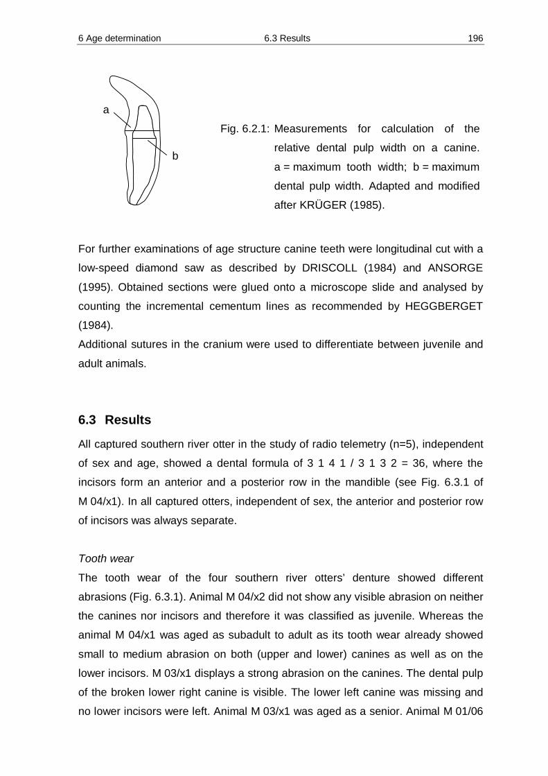
6 Age determination 6.3 Results 196
Fig. 6.2.1: Measurements for calculation of the
relative dental pulp width on a canine.
a = maximum tooth width; b = maximum
dental pulp width. Adapted and modified
after KRÜGER (1985).
For further examinations of age structure canine teeth were longitudinal cut with a
low-speed diamond saw as described by DRISCOLL (1984) and ANSORGE
(1995). Obtained sections were glued onto a microscope slide and analysed by
counting the incremental cementum lines as recommended by HEGGBERGET
(1984).
Additional sutures in the cranium were used to differentiate between juvenile and
adult animals.
6.3 Results
All captured southern river otter in the study of radio telemetry (n=5), independent
of sex and age, showed a dental formula of 3 1 4 1 / 3 1 3 2 = 36, where the
incisors form an anterior and a posterior row in the mandible (see Fig. 6.3.1 of
M 04/x1). In all captured otters, independent of sex, the anterior and posterior row
of incisors was always separate.
Tooth wear
The tooth wear of the four southern river otters’ denture showed different
abrasions (Fig. 6.3.1). Animal M 04/x2 did not show any visible abrasion on neither
the canines nor incisors and therefore it was classified as juvenile. Whereas the
animal M 04/x1 was aged as subadult to adult as its tooth wear already showed
small to medium abrasion on both (upper and lower) canines as well as on the
lower incisors. M 03/x1 displays a strong abrasion on the canines. The dental pulp
of the broken lower right canine is visible. The lower left canine was missing and
no lower incisors were left. Animal M 03/x1 was aged as a senior. Animal M 01/06
a
b

6 Age determination 6.3 Results 197
also showed strong abrasion on the mandibular incisors and the canine including
dental pulp exposure. M 01/06 is therefore also aged as senior.
Fig. 6.3.1: Abrasion of incisors and canines for four southern river
otters. M = male, followed by year, x = died in captivity; following / = radio transmitter channel of radio tracked animal. Darker shading of right upper canine of M 04/x1 results from extracting before otter skull was prepared
Dental pulp
All four X-rayed canines showed different dental pulp width (Appendix 10.5;
Tab. A). The largest dental pulp width was measured in the canine of M 04/x2 at
5.17 mm , followed by M 04/x1 at 1.92 mm , for this reason they were aged as
juvenile and subadult – adult respectively. We classified M 03/x1 with 1.44 mm
and M 01/06 with 1.04 mm as seniors as they showed lowest dental pulp width.
Additionally the decrease in abrasion of the tip of the canine (from left to right) can
be seen (see Fig. 6.3.2). Relative width of dental pulp is presented in Tab. 6.3.1
where all results are summarised.
M 01/06 M 03/x1
M 04/x1 M 04/x2
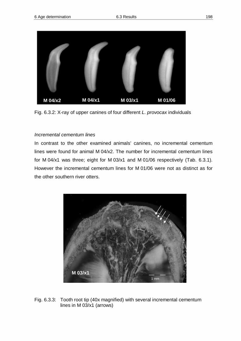
6 Age determination 6.3 Results 198
Fig. 6.3.2: X-ray of upper canines of four different L. provocax individuals
Incremental cementum lines
In contrast to the other examined animals’ canines, no incremental cementum
lines were found for animal M 04/x2. The number for incremental cementum lines
for M 04/x1 was three; eight for M 03/x1 and M 01/06 respectively (Tab. 6.3.1).
However the incremental cementum lines for M 01/06 were not as distinct as for
the other southern river otters.
Fig. 6.3.3: Tooth root tip (40x magnified) with several incremental cementum lines in M 03/x1 (arrows)
1 mm M 03/x1
M 04/x2 M 04/x1 M 03/x1 M 01/06

6 Age determination 6.3 Results 199
Sutures of skull
Only the skull of animal M 04/x2 showed patent sutures (Appendix 10.5;
Fig. A, B, C) and was aged as juvenile. The other three skulls were classified as
adults. Furthermore, the skull of M 03/x1 showed a shot gun pellet in the mandible
which was already incorporated prior to death. New calcification is visible around
the impact area and the shot gun pellet was coated with a thin calcification layer. It
is assumed that the mandibular trauma occurred at juvenile or subadult state.
Tab. 6.3.1: Measurements of tooth wear, increment cementum layers and relative width of dental pulp
Animal Tooth wear age class
Incremental cementum lines
Relative width of dental pulp in %
Resulting age estimation
M 04/x2 1 0 66.7 Juvenile
M 04/x1 2 3 24.8 Subadult – Adult
M 03/x1 3 8 18.1 Senior
M 01/06 3 8 12.8 Senior

6 Age determination 6.4 Discussion 200
6.4 Discussion
As age determination can provide an inside into the demography of species, four
methods were verified. However, there are some restrictions regarding the findings
of analysed individuals. Results of age determination can statistically not be
tested, as the samples were limited to only four individuals and only male animals
were examined.
Morphological features such as body size and weight, cannot be used for age
estimation as juvenile to subadult male southern river otters can attain the size
and weight of adult females or old animals (termed here as seniors) which will
have lost weight.
Tooth wear
Age determination by tooth wear is the easiest method and the most common
criteria for age classification used on mammals (KRÜGER, 1995). The crown of
the teeth is covered by enamel, which can show some age related changes, like
loss in permeability, an increase in brittleness and abrasion which results in an
irreversible loss of enamel (VANDEVOORT et al., 2004).
Lontra provocax showed abrasion according to their age but there may be
individual variations due to differences between habitat and populations, which
can result in errors as is known for other mammals (ANSORGE & STUBBE, 1995;
FIERO & VERTS, 1986; HARRIS, 1978; STANDER, 1997). For red foxes
Vulpes vulpes and badgers Meles meles (VAN BREE et al., 1974) as well as for
gray fox Urocyon cinereoargenteus (NICHOLSON & HILL, 1986) the concordance
of tooth wear estimate and other age criteria were significantly different. Likewise
tooth eruption and consequential tooth wear can vary significantly intersexually
(SMUTS et al., 1978).
Two L. provocax dentitions (M 03/x1; M 01/06) show tooth fracture of their canine
teeth. Tooth breakage is normal and is infrequently accompanied by severe
pathologies in lions Panthera leo (PATTERSON et al., 2003). According to VAN
VALKENBURGH (1988), most commonly broken teeth are canines and more than
25 percent of various carnivores have broken teeth during their life, which is a
function of age, feeding pressure and meat consumption that includes bones. An
intersexual difference was found by STANDER (1997) as a higher frequency of
broken canines in male leopards Panthera pardus than females were observed.
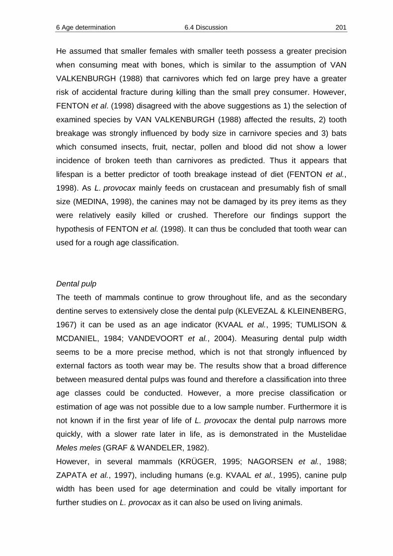
6 Age determination 6.4 Discussion 201
He assumed that smaller females with smaller teeth possess a greater precision
when consuming meat with bones, which is similar to the assumption of VAN
VALKENBURGH (1988) that carnivores which fed on large prey have a greater
risk of accidental fracture during killing than the small prey consumer. However,
FENTON et al. (1998) disagreed with the above suggestions as 1) the selection of
examined species by VAN VALKENBURGH (1988) affected the results, 2) tooth
breakage was strongly influenced by body size in carnivore species and 3) bats
which consumed insects, fruit, nectar, pollen and blood did not show a lower
incidence of broken teeth than carnivores as predicted. Thus it appears that
lifespan is a better predictor of tooth breakage instead of diet (FENTON et al.,
1998). As L. provocax mainly feeds on crustacean and presumably fish of small
size (MEDINA, 1998), the canines may not be damaged by its prey items as they
were relatively easily killed or crushed. Therefore our findings support the
hypothesis of FENTON et al. (1998). It can thus be concluded that tooth wear can
used for a rough age classification.
Dental pulp
The teeth of mammals continue to grow throughout life, and as the secondary
dentine serves to extensively close the dental pulp (KLEVEZAL & KLEINENBERG,
1967) it can be used as an age indicator (KVAAL et al., 1995; TUMLISON &
MCDANIEL, 1984; VANDEVOORT et al., 2004). Measuring dental pulp width
seems to be a more precise method, which is not that strongly influenced by
external factors as tooth wear may be. The results show that a broad difference
between measured dental pulps was found and therefore a classification into three
age classes could be conducted. However, a more precise classification or
estimation of age was not possible due to a low sample number. Furthermore it is
not known if in the first year of life of L. provocax the dental pulp narrows more
quickly, with a slower rate later in life, as is demonstrated in the Mustelidae
Meles meles (GRAF & WANDELER, 1982).
However, in several mammals (KRÜGER, 1995; NAGORSEN et al., 1988;
ZAPATA et al., 1997), including humans (e.g. KVAAL et al., 1995), canine pulp
width has been used for age determination and could be vitally important for
further studies on L. provocax as it can also be used on living animals.

6 Age determination 6.4 Discussion 202
Incremental cementum lines
In several mammals over the past decades age determination using incremental
cementum lines has been carried out. First enumerations of annuli lines were done
on cervids (EIDMANN, 1933) where annual lines were easily identifiable. For
carnivores it is more difficult to achieve meaningful results and some methods
include the decalcification of the tooth (BODKIN et al., 1997). Furthermore the
interpretation of the incremental cementum lines needs experience and verification
should be done by more than one person (pers. comm., ANSORGE).
On several otter species age determination by incremental cementum lines has
already been applied, for example European otter Lutra lutra (e.g. HAUER et al.,
2002; HEGGBERGET, 1984), sea otter Enhydra lutris (e.g. BODKIN et al., 1997;
GARSHELIS, 1984) and Northern river otter Lontra canadensis (e.g. BAITCHMAN
& KOLLIAS, 2000; GROVE et al., 2003; STEPHENSON, 1977). The results show
that incremental cementum lines exist and are different in number. Based on the
results a rough classification was conducted. Line formation seems to be analogue
to the European otter L. lutra (HEGGBERGET, 1984) and L. canadensis
(STEPHENSON, 1977). However, as no data exists on incremental cementum
lines of L. provocax, it is not known if the lines are formed annually and represent
life years. Presuming cementum lines represent annual lines, the two adult
southern river otters (seniors) reached an age of eight years.
For verification if cementum lines are formed annually calciphilic biomarkers such
as tetracycline can be used (JOHNSTON et al., 1987). That means animals have
to be held in captivity, or wild animals, which are captured as juveniles, have to be
recaptured. On recaptured animals the vestigial single-rooted first premolar could
be removed and age determined as GARSHELIS (1984) and BODKIN et al.
(1997) described for E. lutris. However, it still has to be proven whether the first
premolar is suitable for age determination in L. provocax. Furthermore the capture
of this species is very difficult and planned recapture almost impossible.
Sutures of skull
The otter skulls have only been used to distinguish between juvenile and adult
animals. No differences in sutures were found between subadult – adult to seniors.
We estimate the age of M 04/x1 at 6 – 7 months, as juveniles stay first months in
den and were usually first seen in August – September and this otter was trapped

6 Age determination 6.4 Discussion 203
at the beginning of February. Furthermore I assume that the juvenile southern river
otter already had a permanent dentition, as at 5 months all permanent teeth were
developed in L. lutra (HEGGBERGET & CHRISTENSEN, 1996).
In conclusion, the applied methods show promising results as all four individuals
can be classified by each method, i.e. tooth wear, dental pulp, incremental
cementum lines and sutures of skull into the same age class. However, suture
method can only be used to determine between the juvenile and adult stage.
More material is needed for statistical procedures and for a more precise age
classification an animal with known age has to be investigated.

7 Summary 204
7 Summary The southern river otter Lontra provocax belongs to the genus Lontra (American
river otters) and is distributed along southern Chile and Argentina. The southern
river otter, once widely distributed in Chile, is today in freshwater habitats limited to
only few isolated areas. The southern river otter is listed in CITES Appendix I; in
the EU by law 338/97 in Annex A; and in the IUCN Red List of vertebrates as
‘endangered’.
The conducted study presents for the first time substantial data and analyses on
preferred habitat components, activity pattern, prey availability, diet composition
and potential food competitors, as well as a first attempt in age determination,
which is essential for demographic studies. The principle aim of the study is to
gain knowledge of the behaviour and the factors which may effect the distribution
and abundance of the southern river otter.
Three southern river otter, two female and one male, were successful equipped
with radio transmitter and radio tracked. Both female southern river otters were
classified as resident, as they met the asymptote for home range stabilisation.
However the male southern river otter was classified as temporary resident, as he
stayed for 4 months in the study area and then disappeared.
As only the home range of one female was accessible for a habitat composition
survey, her preferred habitat structures were analysed. Thus the plant Quila
Chusquea quila is most important for den sites in anthropogenic modified areas,
as it is very dense and provides protection. Two accidentally found dens in the
ombrophilous swamp forest were encountered under big trees and overhanging
roots. Therefore it is assumed that vegetation type for den sites depends upon the
degree of anthropogenic influence.
The investigated hunting areas in the anthropogenic modified region had
considerably more woody debris than in non-hunting areas. This can be explained
by the use of woody debris by the crayfish Samastacus spinifrons, the main prey
of L. provocax, which hides in this substrate. Furthermore the appearance of the
substrate gravel is correlated with woody debris, and this provides hiding places
for Aegla abtao, another crustacean species that L. provocax preys upon.
7 Summary 205
Investigations of marking sites used by L. provocax show that latrines close to the
water line and in conspicuous and open vegetation structures, such as soil/stones
and grass/herbs, were preferred, as other southern river otters may be able to find
these markings easily. Most of their time southern river otter spent in dens (60 %). When being active, the
time bouts of movement behaviour averaged 2:18 hours and the distance covered
in that time averaged 914 m. By analysing the activity pattern of L. provocax,
cathemeral behaviour was detected. However, the predominant reason for
cathemeral activity cannot be identified in the present study.
As one female southern river otter gave birth in the time of investigations, her
activity pattern and home range changed. In the postnatal period home range was
reduced and undisturbed tributaries were used. As the cubs aged, all river
sections previously used by the mother were visited regularly. The activity pattern
of the female with cubs changed significantly, as she spent time outside of the den
more frequently.
Amphibian samplings and electrofishing was carried out in the study area to
determine potential prey species and prey availability, taking into consideration the
influencing factors, for the southern river otter. To draw conclusions of diet
composition, competition and seasonal changes, 606 faecal samples of
L. provocax and 24 of M. vison were analysed.
Amphibian diversity and abundance was low due to strong anthropogenic modified
area and resultant inadequate amphibian habitats. The crustacean species
S. spinifrons was the most encountered aquatic prey species in abundance and in
total biomass in the investigated river. For the occurrence of S. spinifrons the river
bed composition of woody debris as well as trees/roots was most important.
Flooding seems to influence prey availability negatively, as abundance and
biomass of aquatic species decreased significantly after this occurred.
The investigated river is characterized by its low hardness, low conductivity but
high oxygen concentration. Even in water samples taken close to villages,
physico-chemical parameter values were well below critical or toxic levels on
aquatic species. However, due to the low buffer capacity of the river, it is sensitive
to any changes which may increase the pH-value and threat egg and larvae
development of fishes.
7 Summary 206
The diet of L. provocax consisted mainly of crustaceans, with a minor element of
fish, which significant increase during the wet season. Even only few faeces with
fish remains were detected, it is assumed that the southern river otter consumes
fish regularly, as the animal would need to consume for its daily basic metabolic
requirements on average 318 individuals of S. spinifrons. Faeces with fish remains
may not be used for marking, as it is more ephemeral than faeces which contain
crustacean remains.
The only possible food competitor for L. provocax which occurs in the study area is
the American mink Mustela vison. However, a lack of food competition between
L. provocax and M. vison is suggested, as compared food sources of both species
demonstrate a relatively low similarity of diet.
Tooth wear; tooth abrasions; dental pulp; relative width of dental pulp, incremental
cementum lines; number of lines, and sutures of the skull; visible sutures were
used for age determination on four southern river otter skulls. By using the
methods tooth wear, incremental cementum lines and relative width of dental pulp
it was possible to classify the animals as juvenile (n=1), subadult-adult (n=1) and
senior (n=2). However, as only the juvenile showed sutures, it was not possible to
distinguish between subadult - adult to senior and therefore sutures on skulls
provide information about age, but have to be used in combination with the other
presented methods for more accurate classification.
In the present study it was possible to highlight and discuss behaviour patterns
and present factors, which are of importance for southern river otter presence.

8 Reference List 207
8 Reference List
ABLES, E. D. (1969). Activity studies of red foxes in southern Wisconsin. Journal of Wildlife Management 33: 145-153.
ADAMS, S. B.; FRISSELL, C. A. & RIEMANN, B. E. (2001). Geography of invasion in mountain streams: Consequences of headwater lake fish introductions. Ecosystems 4 (4): 296-307.
AEBISCHER, N. J.; ROBERTSON, P. A. & KENWARD, R. E. (1993a). Compositional analysis of habitat use from animal radio-tracking data. Ecology 5 (74): 1313-1325.
AEBISCHER, N. J.; ROBERTSON, P. A. & KENWARD, R. E. (1993b). Compositonal analysis of habitat use from animal radio-tracking data. Ecology 5 (74): 1313-1325.
ALEXANDER, M. M. (1958). The place of aging in wildlife management. Am.Sci. 46: 123-137.
ANDERSON, D. J. (1982). The home range: a new nonparmetric estimation technique. Ecology 63: 103-112.
ANDREWS, E. (1989). Assessment of the value of rivers for otters (Lutra lutra). Regulated rivers: Research and Management 4: 199-202.
ANGERMEIER, P. L. & KARR, J. R. (1984). Relationships between woody debris and fish habitat in a small warmwater stream. Transactions of the American Fisheries Society 113: 716-726.
ANOOP, K. R. & HUSSAIN, S. A. (2005). Food and feeding habits of smooth-coated otters (Lutra perspicillata) and their significance to the fish population of Kerala, India. J.Zool., Lond. 266: 15-23.
ANSORGE, H. (1995). Remarks on the age determination by growth lines in the mammalian skull. Methoden feldökol.Säugetierforschung 1: 95-102.
ANSORGE, H. & STUBBE, M. (1995). Nonmetric skull divergence in the otter - assessing genetic insulation of populations. IUCN Otter Spec.Group Bull. 17-30.
APHA (1980). Standard Methods for the Exam of Water and Wastewater. 12th edition. Apha Press, New York.
ARENAS, J. (1978). Análisis de la alimentación de Salmo gairdnieri Richardson en el lago Riñihue y río San Pedro, Chile. Medio Ambiente 3 (2): 50-58.
ARNEMO, J. M. (1990). Medikamentell immobilisiering av europeisk (Lutra lutra). Norsk Veterinærtidsskrift 102 (11): 767-770.

8 Reference List 208
ARONSON, B. D.; BELL-PEDERSEN, D.; BLOCK, G. D.; BOS, N. P. & DUNLAP, J. C. (2003). Circadian rhythms. Brain Res.Brain Res.Rev. 18: 315-333.
BAILEY, T. N. (1974). Social organization in a bobcat population. J.Wildl.Manage. 38 (3): 435-446.
BAITCHMAN, E. J. & KOLLIAS, G. V. (2000). Clinical anatomy of the North American river otter (Lontra canadensis). J.Zoo.Wildl.Med. 31 (4): 473-483.
BALLIET, R. F. & SCHUSTERMAN, R. J. (1971). Underwater and aerial visual acuity in the Asian "clawless" otter (Amblonyx cineria cineria). Nature 234: 305-306.
BARTELT, P. E.; PETERSON, C. R. & KLAVER, R. W. (2004). Sexua differences in the post-breeding movement and habitats selected by western toads (Bufo boreas) southeasten Idaho. Herpetologica 60 (4): 455-467.
BEAMISH, F. W. & JEBBINK, J.-A. (1994). Abundance of lamprey larvae and physical habitat. Environmental Biology of Fishes 39 (2): 209-214.
BEGON, M. E., HARPER, J. L. & TOWNSEND, C. R. (1996). Ökologie. Spektrum Akademischer Verlag, Heidelberg, Berlin, Oxford. 750pp.
BEJA, P. R. (1996). An analysis of otter Lutra lutra predation on introduced american crayfish Procambarus clarkii in Iberian streams. The Journal of Applied Ecology 33 (5): 1156-1170.
BEJA, P. R. (1992). Effects of freshwater availability on the summer distribution of otters Lutra lutra in the southwest coast of Portugal. Ecography 15 (3): 273-278.
BELANT, J. L. & FOLLMANN, E. H. (2002). Sampling considerations for American black and brown bear home range and habitat use. Ursus 13: 299-315.
BELTRÁN, J. F. & DELIBES, M. (1994). Environmental determinants of circadian activity of free-ranging Iberian lynxes. Journal of Mammology 75 (2): 382-383.
BENKE, A. C. (1998). Production of riverine chionomids: extremely high biomass turnover rates of primary consumers. Ecology 79: 899-910.
BLUNDELL, G. M., BOWYER, R. T., BEN-DAVID, M., DEAN, T. A. & JEWETT, S. C. (2000). Effects of food resources on spacing behavior of river otters: does forage abundance control home-range size? In: 15th International Symposium on Biotelemetry. J.H.Eiler, D.J.Alcorn & R.M.Newman (eds.). International Society on Biotelemetry, Wageningen, The Netherlands. pp. 325-333.
BLUNDELL, G. M.; KERN, J. W.; BOWYER, R. T. & DUFFY, L. K. (1999). Capturing river otters: a comparison of hancock and leg-hold traps. Wildlife Society Bulletin 27 (1): 184-192.
8 Reference List 209
BLUNDELL, G. M.; MAIER, J. A. & DEBEVEC, E. M. (2001). Linear home ranges: Effects of smoothing, sample size, and autocorrelation on kernel estimates. Ecological Monographs 71 (3): 469-489.
BODKIN, J. L.; AMES, J. A.; JAMESON, R. J.; JOHNSON, A. M. & MATSON, G. M. (1997). Estimating age of sea otters with cementum layers in the first premolar. J.Wildl.Manage. 61 (3): 967-973.
BOHLIN, T.; HAMRIN, S.; HEGGBERGET, T. G.; RASMUSSEN, G. & SALTVEIT, S. J. (1989). Electrofishing - Theory and practice with special emphasis on salmonids. Hydrobiologia 173: 9-43.
BONESI, L.; CHANIN, P. & MACDONALD, D. W. (2004). Competition between Eurasian otter Lutra lutra and American mink Mustela vison probed by niche shift. OIKOS 106: 19-26.
BOONSTRA, R. & CRAINE, I. T. M. (1986). Natal nest location and small mammal tracking with a spool and line technique. Can.J.Zool. 64: 1034-1036.
BOWYER, R. T.; TESTA, J. W. & FARO, J. B. (1995). Habitat selection and home ranges of river otters in a marine environment: effects of the Exxon Valdez oil spill. Journal of Mammology 76: 1-11.
BRZEZINSKI, M.; JEDRZEJEWSKI, W. & JEDRZEJEWSKA, B. (1993). Diet of otters (Lutra lutra) inhabiting small rivers in the Bialowieza National Park, Poland. J.Zool., Lond. 230: 495-501.
BRZEZINSKI, M. & ZUROWSKI, W. (1992). Spring diet of the American mink Mustela vison in the Mazurian and Brodnica Lakelands, norhtern Poland. Acta Theriologica 37 (1-2): 193-198.
BURT, W. H. (1943). Territoriality and Home Range Concepts as Applied to Mammals. Journal of Mammology 24 (3): 346-352.
BUSKIRK, S. W. & LINDSTEDT, S. L. (1989). Sex biases in trapped samples of Mustelidae. Journal of Mammology 70: 88-97.
CAMPOS, H. & MORENO, C. (1985). Chapter 18 - Asociaciones de peces en estuarios chilenos, pacífico sur americano. In: Fish Community in Estuaries and Coastal Lagoons: Towards an Ecosystem Integration. Yáñez-Arancibia.(ed.). UNAM, Press México. pp. 407-414.
CARSS, D. N. (1995). Foraging behaviour and feeding ecology of the otter Lutra lutra: a selecitve review. Hysterix 7 (1-2): 179-194.
CARSS, D. N.; KRUUK, H. & CONROY, J. W. H. (1990). Predation on adult Atlantic salmon, Salmo salar L., by otters, Lutra lutra (L.), within the River Dee system, Aberdeenshire, Scotland. J.Fish.Biol. 37: 935-944.
CARSS, D. N. & PARKINSON, S. G. (1996). Errors associated with otter Lutra lutra faecal analysis. I. Assessing general diet from spraints. J.Zool., Lond. 238: 301-317.

8 Reference List 210
CASATTI, L.; LANGEANI, F.; SILVA, A. M. & CASTRO, R. M. C. (2006). Stream fish, water and habitat quality in a pasture dominated basin, southeastern Brazil. Braz.J.Biol. 66 (2B): 681-696.
CATLING, P. C.; CORBETT, L. K. & WESTCOTT, M. (1991). Age determination in the dingo and crossbreeds. Wildlife Research 18: 75-83.
CHANIN, P. (1981). The diet of the otter and its relations wiht the feral mink in two areas of Southwest England. Acta Theriologica 26: 83-95.
CHANIN, P. R. F. (1985). The Natural History of Otters. Fact On File Publications, New York.
CHARÁ, J. D.; BAIRD, D. J.; TELFER, T. C. & RUBIO, E. A. (2006). Feeding ecology ad habitat preferences of the catfish genus Trichomycterus in a low-order streams of the Colombian Andes. Journal of Fish and Biology 68 (4): 1026-1040.
CHEHÉBAR, C. E. (1985). A survey of the Southern river otter, Lutra provocax Thomas, in Nahuel Huapi National Park. Argentian. Biological Conservation 32: 299-307.
CHEHÉBAR, C. E.; GALLUR, A.; GIANNICO, G.; GOTTELLIL, M. D. & YORIO, P. (1986). A survey of the southern river otter Lutra provocax in Lanin, Puelo and Los Alerces National Parks, Argentina, and evaluation of its conservation status. Biological Conservation 38: 293-304.
CHEHÉBAR, C. E. & PORRO, G. (1998). Distribución y estatus del huillín (Lontra provocax) en el Parque Nacional Huapi, Argentina. Vida Silvestre Neotropical 7 (2-3): 99-106.
CIANCIO, J. & PASCAL, M. (2006). Energy density of freshwater Patagonian organism. Ecología Austral 16: xxx-xxx in press
CLARKE, J.; JONES, M. & JARMAN, P. (1995). Dirunal and nocturnal grouping and foraging behaviours of free-ranging Eastern grey kangaroos. Aust.J.Zool. 43: 519-529.
CLAVERO, M.; PRENDA, J. & DELIBES, M. (2005). Amphibian and reptile consumption by otters (Lutra lutra) in a coastal area in southern iberian peninsula. Herpetological Journal 15: 125-131.
CLEMENTS, S. P.; HICKS, B. J.; CARRAGHER, J. F. & DEDUAL, M. (2002). The Effect of a Trapping Procedure on the Stress Response of Wild Rainbow Trout. North American Journal of Fisheries Management 22: 907-916.
CLODE, D. & MACDONALD, D. W. (1995). Evidence for food competiton between mink (Mustela vison) and otter (Lutra lutra) on Scottish island. J.Zool., Lond. 237: 435-444.
COPP, G. H. & ROCHE, K. (2003). Range and diet of Eurasian otters Lutra lutra (L.) in the catchment of the River Lee (south-east of England) since re-introduction. Acuatic Conserv: Mar Fresh Ecosyst 13 (1): 65-76.

8 Reference List 211
CORN, P. S. & BURY, R. B. (1990). Sampling methods for terrestral amphibians and reptiles. U.S.Department of Agriculture, Forest Service, Technical Report PNW-GTR-256
CROOK, D. A. & ROBERTSON, A. I. (1999). Relationships between riverine fish and woody debris: implications for lowland rivers. Mar.Freshwater.Res. 50: 941-953.
CURTIS, D. J. & RASMUSSEN, M. A. (2006). The evolution of cathemerality in primates and other mammals: a comparative and chronoecological approach. Folia Primatol 77: 178-193.
DAAN, S. & ASCHOFF, J. (1982). Circadian contribution to survival. In: Vertebrate circadian systems: structure and physiology. J.Aschoff, S.Daan & G.A.Groos (eds.). Springer Verlag, Berlin. pp. 305-321.
DAHLE, B. & SWENSON, J. E. (2003). Seasonal range size in relation to reproductive strategies in brown bears Ursus arctos. Journal of Animal Ecology 72 (4): 660-667.
DALZELL, D. J. B. & MACFARLANE, N. A. A. (1999). The toxicity of iron to brown trout and effects on the gills: a comparison of two grades of iron sulphate. Journal of Fish Biology 55 (2): 301-315.
DAVIS, J. A. (1978). A classification of the otters. In: Proceedings of the first working meeting of the Otter Specialist Group. N.Dublaix.(ed.). International Union for the Conservation of Nature, Gland, Switzerland. pp. 14-33.
DE VILLIERS, P. A. & KOK, O. B. (1997). Home range, association and related aspects of elephants in the eastern Transvaal Lowveld. Afr.J.Ecol. 35: 224-236.
DELIBES, M. & ADRIAN, J. (1987). Effects of crayfish introduction on otter Lutra lutra food in the Doñana National Park, S.W. Spain. Biological Conservation 42: 153-159.
DEMERS, F.; GIROUX, J.-F.; GAUTHIER, G. & BÊTY, J. (2003). Effects of collar-attached transmitters on behaviour, pair bond and breeding success of snow geese Anser caerculescens atlanticus. Wildl.Biol. 9: 77-86.
DIXON, K. R. & CHAPMAN, J. A. (1980). Harmonic mean measure of animal activity areas. Ecology 61: 1040-1044.
DOLLAR, L. (1999). Preliminary report on the status, activity cycle and ranging of Cryptoprocta ferox in the Malagasy rainforest, with implications for conservation. Small Carnivore Conservation (IUCN/SSC Mustelid, Viverrid and Procyonid Specialist Group) 20: 7-10.
DOLLOF, C. A. (1993). Predation by river otters (Lutra canadensis) on juvenile coho salmon (Oncorhynchus kisutch) and dolly varden (Salvelinus malma) in southeast Alaska. Can.J.Fish.Aquat.Sci. 50 (2): 312-315.

8 Reference List 212
DOLLOFF, C. A. (1994). Large woody debris - the common denominator for integrated environmental management of forest streams. In: Integrated environmental management. J.Jr.Cairns, T.V.Crawford & H.Salwasser (eds.). University Center for Environmental and Hazardous Materials Studies, Blacksburg, Virginia 24061. pp. 93-107.
DONCASTER, C. P. & WOODROFFE, R. (1993). Den site can determine shape and size of badger territories: implications for group-living. OIKOS 66: 88-93.
DRISCOLL, K. M.; JONES, G. S. & NICHY, F. (1985). An efficient method by which to determine age of carnivores, using dentine rings. J.Zool., Lond. 205: 309-313.
DRURY, D. M. & KELSO, W. E. (2004). Invertebrate colonization of woody debris in coastal plain streams. Hydrobiologia 434 (1-3): 63-72.
DUNSTONE, N. (1979). Swimming and diving behaviour of the mink (Mustela vison Schreber). Carnivore 2: 56-61.
DUNSTONE, N. & GORMAN, M. L. (1998). Behaviour and Ecology of Riparian Mammals (Symosia of the Zoological Society of London; 71). Cambridge University Press, Cambridge. 391pp.
DURBIN, L. S. (1996). Some changes in the habitat use of a free-ranging female otter Lutra lutra during breeding. J.Zool., Lond. 240: 761-764.
DURBIN, L. S. (1993). Food and habitat utilization of otters (Lutra lutra L.) in a riparian habitat. PhD. University of Aberdeen. 114pp.
DYER, B. S. (2000). Systematic review and biogeography of the freshwater fishes of Chile. Estud.Oceanol. 19: 77-98.
EBEDES, H. & VAN ROOYEN, J. (2002). Chapter 34 - Keeping and feeding wild animals in captivity. In: Game ranch management. 4th edition. J.d.P.Bothma.(ed.). Van Schaik Uitgewers, Pretoria. pp. 441-454.
EBEDES, H., VAN ROOYEN, J. & DU TOIT, J. G. (2002). Chapter 33 - Capturing wild animals. In: Game ranch Management. 4th edition. J.d.P.Bothma.(ed.). Van Schaik Uitgewers, Pretoria. pp. 382-440.
EBENSPERGER, L. A. & BOTTO-MAHAN, C. (1997). Use of habitat, size of prey, and food-niche relationships of two sympatric otters in southernmost Chile. Journal of Mammology 78 (1): 222-227.
EIDMANN, R. (1933). Alterserscheinung am Gebiß des Rothirsches als Grundlage zur exakten Bestimmung des Lebensalters. Verlag M.& H. Schaper, Hannover.
EIFAC (EUROPEAN INLAND FISHERIES ADVISORY COMMISSION) (1969). Water quality criteria for European freshwater fish - extreme pH values and inland fisheries. Water Res. 3: 593-611.

8 Reference List 213
ELVIDGE, H.; CHALLIS, F. R. G.; ROBINSON, J. S.; ROPER, C. & THORBURN, G. D. (1976). Influence of handling and sedation on plasma cortisol in rhesus monkeys (Macaca mulatta). Journal of Endocrinology 70: 325-326.
EMERY, A. R. (1973). Preliminary comparisons of day and night habits of freshwater fish in Ontariolakes. J.Fish.Res.Bd.Can. 30: 761-774.
EMLEN, J. M. (1966). The role of time and energy in food preferences. Am.Nat. 100: 611-617.
ENGELMANN, H.-D. (1971). Zur Dominanzklassifizierung von Bodenarthropoden. Pedobiologia 18: 378-380.
ENRIGHT, J. T. (1970). Ecological aspects of endogenous rhythmicity. Annu.Rev.Ecol.Syst. 1: 221-238.
ERICKSON, D. W. & MCCULLOUGH, C. R. (1987). Fates of translocated otters in Missouri. Wildlife Society Bulletin 15: 511-517.
ERLINGE, S. (1968). Food studies on captive otters Lutra lutra (L.). OIKOS 19: 259-270.
ERLINGE, S. (1972). Interspecific relations between otter Lutra lutra and mink Mustela vison in Sweden. OIKOS 23: 372-335.
ERLINGE, S. (1974). Distribution, territoriality and numbers of the weasel Mustela nivalis in relation to prey numbers. OIKOS 25: 308-314.
ERLINGE, S. (1967). Home range of the otter, Lutra lutra L. in Southern Sweden. OIKOS 18: 186-209.
ERLINGE, S. & SANDELL, M. (1986). Seasonal changes in the social organisation of male stoats, Mustela erminea: an effect of shifts between two decisive resources. OIKOS 47: 57-62.
ESRI. (1996) (Environmental System Research Institute) ArcView GIS (ver.3.2). Readland, California
ESTES, J. A. (1980). Enhydra lutris. MAMMALIAN SPECIES 133: 1-8.
ESTES, J. A. (1989). Adaptations for aquatic living by carnivores. In: Carnivore Behaviour, Ecology and Evolution. 1 edition. J.L.Gittleman.(ed.). Cornell University Press, Ithaca, New York. pp. 242-282.
ESTES, J. A., JAMESON, R. J. & JOHNSON, A. M. (1981). Food selection and some foraging tactics of sea otters. In: Procedings of the worldwide furbearers conference. J.A.Chapman & D.Pursley (eds.). Frostburg, Md. pp. 606-641.
ESTES, J. A.; JAMESON, R. J. & RHODE, E. B. (1982). Activity and prey selection in the sea otter: influence of population status on community structure. The American Naturalist 120: 242-258.
8 Reference List 214
ESTES, J. A.; RIEDMAN, M. L.; STAEDLER, M. M.; TINKER, M. T. & LYON, B. E. (2003). Individual variation in prey selection by sea otters: patterns, causes and implications. Journal of Animal Ecology 72: 144-155.
EVERETT, R. A. & RUIZ, G. M. (1993). Coarse woody debris as a refuge from predation in aquatic communities. Oecologia 93 (4): 475-486.
EWER, R. F. (1973). The Carnivores. Cornell Univ. Press, Ithaca, New York.
FELTHAM, M. J. & MARQUISS, M. (1989). The use of first vertebrae in separating and estimating the size of trout (Salmo trutta) and salmon (Salmo salar) in bone remains. J.Zool., Lond. 219: 113-122.
FENTON, M. B.; WATERMAN, J. M.; ROTH, J. D.; LOPEZ, E. & FIENBERG, S. E. (1998). Tooth breakage and diet: a comparison of bats and carnivores. J.Zool., Lond. 246: 83-88.
FERGUSON, S. H.; TAYLOR, M. K.; BORN, E. W.; ROSING-ASVID, A. & MESSIER, F. (1999). Determinants of home range size for polar bears (Ursus maritimus). Ecol.Lett. 2: 311-318.
FERNANDEZ-DUQUE, E. (2003). Influence of moonlight, ambient temperature, and food availability on the diurnal and nocturnal activity of owl monkeys (Aotus azarai). Behav Ecol Sociobiol 54: 431-440.
FERNÁNDEZ-MORAN, J.; SAAVEDRA, D. & MANTECA-VILANOVA, X. (2002). Reintroduction of the Eurasian otter (Lutra lutra) in norheastern Spain: Trapping, handling, and medical management. Journal of Zoo and Wildlife Medicine 33 (3): 222-227.
FERRERAS, P. & MACDONALD, D. W. (1999). The impact of American mink Mustela vison on water birds in the upper Thames. Journal of Applied Ecology 36: 701-708.
FIEBERG, J. & KOCHANNY, C. O. (2005). Quantifying home-range overlap: the importance of the utilization distribution. Journal of Wildlife Management 69 (4): 1346-1359.
FIERO, B. C. & VERTS, B. J. (1986). Comparison of techniques for estimating age in raccoons. Journal of Mammology 67 (2): 392-395.
FLEMING, P. J. S.; ALLEN, L. R.; BERGHOUT, M. J.; MEEK, P. D.; PAVLOV, P. M.; STEVENS, P.; STRONG, K.; THOMPSON, J. A. & THOMSON, P. C. (1998). The performance of wild-canid traps in Australia: efficiency, selectivity and trap-related injuries. Wildlife Research 25 (3): 327-338.
GARROTT, R. A.; WHITE, G. C.; BARTMANN, R. M. & WEYBRIGHT, D. L. (1986). Reflected signal bias in biotelemetry triangulation systems. J.Wildl.Manage. 50 (4): 747-752.
GARSHELIS, D. L. (1984). Age estimation of living sea otters. J.Wildl.Manage. 48 (2): 456-463.
8 Reference List 215
GARSHELIS, D. L. (2000). Chapter 4 - Delusions in Habitat Evaluation: Measuring Use, Selection, and Importance. In: Research Techniques in Animal Ecology. Controversies and Consequences. L.Boitani & T.K.Fuller (eds.). Columbia University Press, New York. pp. 111-164.
GARSHELIS, D. L.; JOHNSON, A. M. & GARSHELIS, J. A. (1984). Social organization of sea otters in Prince William Sound, Alaska. Can.J.Zool. 62: 637-647.
GARSHELIS, D. L. & PELTON, M. R. (1980). Activity of black bears in the Great Smoky Mountains National Park. Journal of Mammology 61 (1): 8-19.
GEIGER, G.; BRÖMEL, J. & HABERMEHL, H. (1977). Konkordanz verschiedener Methoden der Altersbestimmung beim Rotfuchs (Vulpes vulpes L., 1758). Zeitschrift für Jagdwissenschaft V23 (2): 57-64.
GERELL, R. (1967). Food selection in relation to habitat in mink (Mustela vison Schreber) in Sweden. OIKOS 18: 233-246.
GERICKE, M. D. & HOFMEYR, J. M. (1976). Aetiology and treatment of capture stress and myopathy in springbok, Antidorcas marsupialis. S.Afr.J.Sci. 72: 28
GESE, E. M.; RUFF, R. L. & CRABTREE, R. L. (1996). Foraging ecology of coyotes (Canis latrans): the influence of extrinsic factors and a dominace hierarchy. Canadian Journal of Zoology 74 (5): 769-783.
GILLOUX, I.; GURNELL, J. & SHEPHERDSON, D. (1992). An enrichment device for great apes. Animal Welfare 1: 279-289.
GITTLEMAN, J. L. & HARVEY, P. H. (1982). Carnivore Home-Range Size, Metabolic Needs and Ecology. Behavioral Ecology and Sociobiology 10: 57-63.
GÖLTENBOTH, R. (1995). Die medikamentöse Immobilisation der Zoo- und Wildtiere. In: Krankheiten der Zoo- und Wildtiere. R.Göltenboth & H.G.Klös (eds.). Blackwell Wissenschaftsverlag, Berlin. pp. 3-8.
GOMI, T.; SIDLE, R. C. & SWANSTON, D. N. (2004). Hydrogeomorphic linkages of sediment transport in headwater streams, Maybeso Experimental Forest, southeast Alaska: Hydrogeomorphology. Hydrological processes 18 (4): 667-683.
GOMPPER, M. E. & GITTLEMAN, J. L. (1991). Home range scaling: intraspecific and comparative trends. Oecologia 87: 343-348.
GONZALEZ LAGOS, C. A. (2006). Dieta del huillín (Lontra provocax) en el humedal de Boroa, IX Región, Chile. Título de médico veterinario. Instituto de Zoología, Facultad de ciencias veterinarias, Universidad Austral de Chile. 43pp.

8 Reference List 216
GORI, M.; CARPANETO, G. M. & OTTINO, P. (2003). Spatial distribution and diet of the Neotropical otter Lontra longicaudis in the Iberia Lake (northern Argentina). Acta Theriologica 48 (4): 495-504.
GRAF, M. & WANDELER, A. I. (1982). Altersbestimmung bei Dachsen (Meles meles L.). Rev.suisse Zool. 89 (4): 1017-1023.
GRANT, G. E. & WOLFF, A. L. (1991). Long-term patterns of sediment transport after timber harvest, western Cascade Mountains, Oregon. In: Sediment and stream water quality in changing environment: Trends and explanation. N.E.Peters & D.E.Walling (eds.). Proceedings of the Vienna symposium, IAHS Publ. No. 203, pp. 31-40.
GRANT, J. W. A.; CHAPMAN, C. A. & RICHARDSON, K. S. (1992). Defended versus undefended home range size of carnivores, ungulates and primates. Behavioral Ecology and Sociobiology 31: 149-161.
GRASSMAN, L. I.; TEWES, M. E. & SILVY, N. J. (2005). Ranging, habitat use and activity patterns of binturong Arctictis binturong and yellow-throated marten Martes flavigula in north-central Thailand. Wildl.Biol. 11: 49-57.
GREEN, J.; GREEN, R. & JEFFERIES, D. J. (1984). A radio-tracking survey of otters Lutra lutra on a perthsire river system. Lutra 27: 85-145.
GROVE, R. A.; BILDFELL, R.; HENNY, C. J. & BUHLER, D. R. (2003). Bilateral uric acid nephrolithiasis and ureteral hypertrophy in a free-ranging river otter (Lontra canadensis). Journal of Wildlife Diseases 39 (4): 914-917.
HABIT, E. & VICTORIANO, P. (2005). Peces de agua dulce de la cordillera de la costa. In: Historia, biodiversidad y ecología de los bosques costeros de Chile. C.Smith-Ramirez, J.Arnesto & C.Valdovinos (eds.). Editorial Universitaria, Santiago, Chile. pp. 392-406.
HABIT, E.; VICTORIANO, P. & CAMPOS, H. (2005). Ecología trófica y aspectos reproductivos de Trichomyterus areolatus (Pisces, Trichomycteridae) en ambientes lóticos artificiales. Rev.Biol.Trop. 52 (4): 195-210.
HAJKOVA, P.; ROCHE, K. & KOCIAN, L. (2003). On the use of diagnostic bones of brown trout, Salmo trutta m. fario, grayling, Thymallus thymallus, and Carpathian sculpin, Cottus poecilopus in Eurasian otter, Lutra lutra diet analysis. Folia Zool. 52 (4): 389-398.
HALLE, S. (2000). Ecological relevance of daily activity patterns. In: Activity patterns in small mammals. An ecological approach. S.Halle & N.C.Stenseth (eds.). Springer, Berlin, Heidelberg, New York. pp. 67-90.
HAMMERSHOJ, M.; THOMSEN, E. A. & MADSEN, A. B. (2004). Diet of free-ranging American mink and European polecat in Denmark. Acta Theriologica 4 (3): 337-347.
HANSON, J. M.; CHAMBERS, P. A. & PREPAS, E. E. (1990). Selective foraging by the crayfish Orconectes virilis and its impact on macroinvertebrates. Freshwater Biology 24 (1): 69-80.
8 Reference List 217
HARDISTY, M. W. & POTTER, I. C. (1971). The behaviour, ecology and growth of larval lampreys. Academic Press, London.
HARRIS, C. J. (1968). Otters a study of the recent Lutrinae. Weidenfeld & Nicolson, 397pp.
HARRIS, S. (1978). Age determination in the red fox (Vulpes vulpes) - an evaluation of technique efficiency as applied to a sample of suburban foxes. J.Zool., Lond. 184: 91-117.
HARRIS, S.; CRESSWELL, W. J.; FORDE, P. G.; TREWHELLA, W. J.; WOOLLARD, T. & WRAY, S. (1990). Home-range analysis using radio-tracking data - a review of problems and techniques particularly as applied to the study of mammals. Mammal Review 20: 97-123.
HARVEY, M. J. & BARBOUR, R. W. (1965). Home range of Microtus ochraogaster as determined by a modified minimum area method. Journal of Mammology 46: 398-402.
HATLAPA, H. & WIESNER, H. (1982). Die Praxis der Wildtierimmobilisation. Pareys, Hamburg, Berlin. 96pp.
HATTINGH, J. (1992). Stress measurement in animals. In: The use of tranquillizers in wildlife. H.Ebedes.(ed.). Department of Agriculture Development, Pretoria. pp. 11-12.
HAUENSTEIN, E.; GONZALEZ, M.; PENA-CORTES, F. & MUÑOZ-PEDREROS, A. (2002). Clasificacion y caracterizacion de la flora y vegetation de los humedales de la costa de Tolten (IX Region, Chile). Gayana Bot. 59 (2): 87-100.
HAUER, S.; ANSORGE, H. & ZINKE, O. (2002). Mortality patterns of otters (Lutra lutra) from eastern Germany. J.Zool., Lond. 256: 361-368.
HAUFLER, J. B. & SERVELLO, F. A. (1996). Chapter 12 - Techniques for Wildlife Nutritional Analyses. In: Research and management techniques for wildlife and habitats. 5th edition. T.A.Bookhout.(ed.). The Wildlife Society, Bethesda, Md. pp. 307-323.
HAWLEY, V. D. & NEWBY, F. E. (1957). Marten home ranges and population fluctuations. Journal of Mammology 38 (2): 174-184.
HEGGBERGET, T. M. (1984). Age determination in the European otter Lutra lutra lutra. Z.Säugetierkunde 49: 299-305.
HEGGBERGET, T. M. (1995). Food resources and feeding ecolgy of marine feeding otters (Lutra lutra). In: Ecology of fjords and coastal waters. H.R.Skjoldal, C.Hopkins, K.E.Erikstad & H.P.Leinaas (eds.). Elsevier, Leiden. pp. 609-618.
HEGGBERGET, T. M. & CHRISTENSEN, H. (1996). Reproductive timing in Eurasian otters on the coast of Norway. Ecography 17: 339-348.
8 Reference List 218
HEGGBERGET, T. M. & MOSEID, K. E. (1994). Prey selection in coastal Eurasian otters Lutra lutra. Ecography 17: 331-338.
HERFINDAL, I.; LINNELL, J. D. C.; ODDEN, J.; BIRKELAND NILSEN, E. & ANDERSON, R. (2005). Prey density, environmental productivity and home-range size in the Eurasian lynx (Lynx lynx). J.Zool., Lond. 265: 63-71.
HERNANDEZ-DIVERS, S.; KOLLIAS, G. V.; ABOU-MADI, N. & HARTUP, B. K. (2001). Surgical technique for intra-abdominal radiotransmitter placement in north american river otters (Lontra canadensis). Journal of Zoo and Wildlife Medicine 32 (2): 202-205.
HILDERBRAND, R. H.; LEMLY, A. D.; DOLLOFF, C. A. & HARPSTER, K. L. (1997). Effects of large woody debris placement on stream channels and benthic macroinvertebrates. Can.J.Fish.Aquat.Sci. 54 (4): 931-939.
HILL, R. A. (2006). Why be diurnal? Or, why not be cathemeral? Folia Primatol 77 (1-2): 72-86.
HOOGE, P. N. and EICHENLAUB, B. (2000b) Animal movement extension to Arcview (ver.2.0). Alaska Science Center - Biological Science Office, U.S. Geological Survey, Anchorage, AK, USA
HOOGE, P. N. and EICHENLAUB, B. (2000a) Animal movement extension to ArcView (ver.2.0). Alaska Science Centre - Biological Science Office, U.S. Geological Survey, Anchorage, AK, USA
HOOVER, J. P. (1984). Surgical implantations of radiotelemetry devices in American river otters. J.Am.Vet.Med.Assoc. 185: 1317-1320.
HORNER, M. A. & POWELL, R. A. (1990). Internal stucture of home ranges of black bears and analyses of overlap. Journal of Mammology 71: 402-410.
HOSEY, G. R. (2006). Zoo animals and their human audiences: what is the visitor effect? Anim.Welf. 9: 343-357.
HUTCHINGS, M. R. & WHITE, P. C. L. (2000). Mustelid scent-marking in managed ecosystems: implications for population management. Mammal Review 30: 157-169.
IUCN (2004). 2004 IUCN Red List of Threatened Species. < www.iucnredlist.org >. Downloaded on: 28 February 2006.
JACKSON, S.; DUFFY, D. C. & JENKINS, J. F. G. (1987). Gastric digestion in marine vertebrate predators: in vitro standards. Functional Ecology 1: 287-291.
JACOBSEN, L. & HANSEN, H.-M. (1996). Analysis of otter (Lutra lutra) spraints: Part 1: Comparison of methods to estimate prey proportions; Part 2: Estimation of the size of prey fish. J.Zool., Lond. 238: 167-180.

8 Reference List 219
JAEGER, R. G.; KALVARSKY, D. & SHIMUYU, N. (1982). Territorial behaviour of the red-backed salamander: Expulsion of intruders. Animal Behaviour 30: 490-496.
JAMESON, R. J. (1989). Movements, home range, and territories of male sea otters off central California. Mar.Mamm.Sci. 5: 159-172.
JARA, C.; RUDOLPH, E. H. & GONZÁLEZ, E. (2006). Estado de conocimiento de los malacostraceos dulceacuicolas de Chile. Gayana 70 (1): 40-49.
JEDREZEJEWSKI, W.; JEDREZEJEWSKA, B. & SZYMURA, A. (1989). Food niche overlaps in a winter community of predators in the Bialowieza Primeval Forest, Poland. Acta Theriologica 34: 487-496.
JEDRZEJEWSKA, B.; SIDOROVICH, V. E.; PIKULIK, M. M. & JEDRZEJEWSKI, W. (2001). Feeding habits of the otter and the American mink in Bialowieza Primeval Forest (Poland) compared to other Eurasian populations. Ecography 24: 165-180.
JENKINS, D. (1980). Ecology of otters in northern Scotland I. Otter (Lutra lutra) breeding and dispersion in Mid-Deeside, Aberdeenshire in 1974-79. Journal of Animal Ecology 49: 713-735.
JENKINS, D. & HARPER, R. J. (1980). Ecology of otters in northern Scotland. 2. Analyses of otter (Lutra lutra) and mink (Mustela vison) faeces from Deeside, N.E. Scotland in 1977-78. Journal of Animal Ecology 49: 755-774.
JENNRICH, R. I. & TURNER, F. B. (1969). Measurement of non-circular home range. Journal of Theoretical Biology 22: 227-237.
JOHNSON, D. D. P.; MCDONALD, D. W. & DICKMAN, A. J. (2000). An analysis and review of models of the sociobiology of the Mustelidae. Mammal Review 30 (Nos 3 & 4): 171-196.
JOHNSON, D. H. (1980). The comparison of usage and availability measurements for evaluating resource preference. Ecology 61 (1): 65-71.
JOHNSTON, D. H., JOACHIM, D. G., BACHMANN, P., KARDONG, K. V., STEWART, R. E. A., DIX, L. M., STICKLAND, M. A. & WATT, I. D. (1987). Chapter 22 - Aging furbearers using tooth structure and biomarkers. In: Wild Furbearer Management and Conservation in North American. M.Novak, J.A.Baker, M.E.Obbard & B.Malloch (eds.). Ministry of Natural Resources, Toronto, Ontario. pp. 228-243.
JORDAN, M. J. R. (2005). Dietary analysis for mammals and birds: a review of field techniques and animal-management applications. International Zoo Yearbook 39 (1): 108-116.
JOWETT, I. G. & RICHARDSON, J. (1995). Habitat preferences of common, riverine New Zealand native fishes and implications for flow management. New Zealand Journal of Marine and Freshwater Research 29: 13-23.
8 Reference List 220
JOWETT, I. G. & RICHARDSON, J. (1996). Distribution and abundance of freshwater fish in New Zealand rivers. New Zealand Journal of Marine and Freshwater Research 30: 239-255.
KAIL, J. (2005). Geomorphic effects of large wood in streams and rivers and its use in stream restoration: A Central European perspective. PhD. Universität Duisburg-Essen. 160pp.
KAPPELER, P. M. & ERKERT, H. G. (2003). On the move around the clock: correlates and determinants of cathemeral activity in the wild redfronted lemurs (Eulemur fulvus rufus). Behav Ecol Sociobiol 54: 359-369.
KATAJISTO, J. & MOILANEN, A. (2006). Kernel-based home range method for data with irregular sampling intervals. Ecological Modelling 194 (4): 405-413.
KAUHALA, K. & TIILIKAINEN, T. (2002). Radio location error and the estimates of home range size, movements, and habitat use: a simple field test. Ann.Zool.Fennici 39: 317-324.
KAVANAU, J. L. & RAMOS, J. (1975). Influences of light on activity and phasing of carnivores. The American Naturalist 109 (968): 392-418.
KEDZIERSKI, W. M. & SMOCK, L. A. (2001). Effects of logging on macroinvertebrate production in a sand-bottomed, low-gradient stream. Freshwater Biology 46: 821-833.
KELLY, F. L. & KING, J. J. (2001). A review of the ecology and distribution of three lamprey species, Lampetra fluviatilis (L.), Lampetra planeri (Bloch) and Petromyzon marinus (L.): a context for conservation and biodiversity consideration in Ireland. Biology and Environment: Proceedings of the Royal Irish Academy 101B (3): 165-185.
KENWARD, R. E. (1987). Wildlife radio tagging. Academic Press, London. 222pp.
KENWARD, R. E.; WALLS, S. S. & HODDER, K. H. (2001). Life path analysis: scaling indicates priming effects of social and habitat factors on dispersal distances. Journal of Animal Ecology 70: 1-13.
KERLEY, L. L.; GOODRICH, J. M.; MIQUELLE, D. G.; SMIRNOV, E. N.; QUIGLEY, H. B. & HORNOCKER, M. G. (2002). Effects of roads and human disturbance on Armur tigers. Conservation Biology 16 (1): 97-108.
KERNOHAN, B. J., GITZEN, R. A. & MILLSPAUGH, J. J. (2001). Chapter 5 - Analysis of animal space use and movements. In: Radio tracking and animal populations. J.J.Millspaugh & J.M.Marzluff (eds.). Academic Press, San Diego, California, USA. pp. 125-166.
KING, C. M. (1975). The home range of the weasel (Mustela nivalis) in an English woodland. Journal of Animal Ecology 44: 639-668.
8 Reference List 221
KLEVEZAL, G. A. and KLEINENBERG, S. E. (1967). Age determination of mammals from annual layers in teeth and bones. (in Russian - translation by Israel Program for Scientific Translation, Jerusalem 1969) .
KLOSKOWSKI, J. (1999). Otter Lutra lutra predation in cyprinid-dominated habitats. Z.Säugetierkunde 64: 201-209.
KLOSKOWSKI, J.; GRENDEL, A. & WRONKA, M. (2000). The use of fish bones of three farm fish species in diet analysis of the Eurasian otter, Lutra lutra. Folia Zool. 49 (3): 183-190.
KOEPFLI, K.-P. & WAYNE, R. K. (1998). Phylogenetic relationships of otters (Carnivora: Mustelidae) based on mitochondrial cytochrome b sequences. J.Zool., Lond. 246: 401-416.
KOLOZSVARY, M. B. & SWIHART, R. K. (1999). Habitat fragmentation and the distribution of amphibians: patch and landscape correlates in farmland. Can.J.Zool. 77 (8): 1288-1299.
KÖRTNER, G. & GEISER, F. (2000). Torpor and activity patterns in free-ranging sugar gliders Petaurus breviceps (Marsupialia). Oecologia 123: 350-357.
KREBS, C. J. (1994). Ecology: the experimental Analysis of Distribution and Abundance. 4th edition. Harper Collins College Publishers, New York. 801pp.
KREBS, C. J. (1998). Ecological Methodology. Benjamin/Cummings, Menlo Park, CA 94025. 620pp.
KRÜGER, H. H. (1995). Zur Populationsstruktur und Morphologie des Baummarders (Martes martes L., 1758) und Steinmarders (Martes foina Erxl., 1777). PhD. Georg-August-Universität zu Göttingen. 133pp.
KRUUK, H. (1992). Scent marking by otters (Lutra lutra): signaling the use of resources. Behavioral Ecology 3 (2): 133-140.
KRUUK, H. (1995). Wild Otters - Predation and Populations. Oxford University Press, Oxford. 290pp.
KRUUK, H.; CONROY, J. W. H. & GLIMMERVEEN, U. (1986). The use of spraints to survey populations of otters (Lutra lutra). Biological Conservation 33: 187-194.
KRUUK, H.; CONROY, J. W. H. & MOORHOUSE, A. (1987). Seasonal reproduction, mortality and food of otters (Lutra lutra L.) in Shetland. Symp.zool.Soc.Lond. 58: 263-278.
KRUUK, H. & MOORHOUSE, A. (1990). Seasonal and spatial differences in food selection by otters (Lutra lutra) in Shetland. J.Zool., Lond. 221: 621-637.
KRUUK, H.; MOORHOUSE, A.; CONROY, J. W. H.; DURBIN, L. S. & FREARS, S. (1989). An estimate of numbers and habitat preferences of otters Lutra lutra in Shetland. UK. Biological Conservation 49: 241-254.

8 Reference List 222
KUMMER, H. (1968). Social organization of hamadryas baboons. The University of Chicago Press, Chicago. 189pp.
KVAAL, S. I.; KOLLTVEIT, K. M.; THOMSEN, I. O. & SOLHEIM, T. (1995). Age estimation of adults from dental radiographs. Forensic Science International 74 (3): 175-185.
LAIR, H. (1987). Estimating the location of the focal center in red squirrel home ranges. Ecology 68: 1092-1101.
LAMOUROUX, N.; CAPRA, H.; POUILLY, M. & SOUCHON, Y. (1999). Fish habitat preferences in large streams of southern France. Freshwater Biology 42 (4): 673-687.
LANSZKI, J.; MOLNÁR, M. & MOLNÁR, T. (2006). Factores affecting the predation of otter (Lutra lutra) on European pond turtle (Emys orbicularis). Journal of Zoology 270: 219-226.
LARA, A. C. & ARAVENA, J. C. (1997). La conservación del bosque nativo en Chile: problemas y desafío. In: Ecología de los Bosques Nativos de Chile. J.J.Armesto, C.Villagrán & M.K.Arroyo (eds.). Editorial Universitaria, Santiago de Chile. pp. 335-362.
LARIVIÈRE, S. (2001). Aonyx capensis. MAMMALIAN SPECIES 671: 1-6.
LARIVIÈRE, S. (1999b). Lontra provocax. MAMMALIAN SPECIES 610: 1-4.
LARIVIÈRE, S. (1999a). Lontra longicaudis. MAMMALIAN SPECIES 609: 1-5.
LARIVIÈRE, S. (1998). Lontra felina. MAMMALIAN SPECIES 575: 1-5.
LARIVIÈRE, S. & WALTON, L. R. (1998). Lontra canadensis. MAMMALIAN SPECIES 587: 1-8.
LARSON, D. G. & GAUTHIER, D. A. (1989). Effects of capturing pregnant muse and calves on calf survivorship. J.Wildl.Manage. 53: 564-567.
LAVER, P. (2005). Abode - User Manual (Beta v.2). 62pp.
LAWS, R. M. (1952). A new method of age determination for mammals. Nature 169: 972-973.
LAWSON, E. J. G. & RODGERS, A. R. (1997). Differences in home-range size computed in commonly used software programs. Wildlife Society Bulletin 25 (3): 721-729.
LE CREN, E. D. (1951). The length-weight relationship and seasonal cycle in gonad weight and condition in the perch Perca fluviatilis. Journal of Animal Ecology 20: 201-219.
LE MUNYAN, C. D.; WHITE, W.; NYBERT, E. & CHRISTIAN, J. J. (1959). Design of a miniature radio transmitter for use in animal studies. Journal of Wildlife Management 23: 107-110.
8 Reference List 223
LEMLY, A. D. & HILDERBRAND, R. H. (2000). Influence of large woody debris on stream insect communities and benthic detritus. Hydrobiologia 421 (1): 179-185.
LEWIS, J. (1991). Reversible inmobilisation of Asian small-clawed otters with medetomidine and ketamine. Veterinary Record 128: 86-87.
LINDSTEDT, S. L.; MILLER, B. J. & BUSKIRK, S. W. (1986). Home range, time, and body size in mammals. Ecology 67 (2): 413-418.
LITVAITIS, J. (2000). Chapter 5 - Investigating food habits of terrestrial vertebrates. In: Research techniques in animal ecology: controversies and consequences. 2 edition. L.Boitani & T.K.Fuller (eds.). Colombia University press, New York. pp. 165-190.
LOCKWOOD, J. L., HOOPES, M. F. & MARCHETTI, M. P. (2007). Invasion ecology. 1st edition. Blackwell Publishing, 304pp.
LODÉ, T. (1995). Activity pattern of polecats Mustela putorius L. in relation to food habits and prey activity. Ethology 100: 295-308.
LÖSCHER, W. (2002). Pharmaka mit Wirkung auf das Zentralnervensystem. In: Grundlagen der Pharmkotherapie bei Haus- und Nutztieren. 5 edition. W.Löscher, F.R.Ungemach & R.Kroker (eds.). Parey Buchverlag, Berlin. pp. 52-105.
LUCHERINI, M. & LOVARI, S. (1996). Habitat richness affects home range size in red fox Vulpes vulpes. Behavioural processes 36 (1): 103-105.
LUSK, C. H. (2001). When is a gap not a gap? Light levels and leaf area index in bamboo-filled gaps in a chilean rain forest. Gayana Bot. 58 (1): 25-30.
MACDONALD, D. W. (1983). The ecology of carnivore social behaviour. Nature 301: 379-384.
MACDONALD, D. W. (1980). Patterns of scent marking with urine and faeces amongst carnivore communities. In: Olfaction in mammals. D.M.Stoddart.(ed.). Academic Press, London. pp. 107-135.
MACE, G. M. & HARVEY, P. H. (1983). Energetic constraints on home range size. Am Nat 121: 120-132.
MAGIN, C. D., JOHNSON, T. H., GROOMBRIDGE, B., JENKINS, M. & SMITH, H. (1994). Chapter 1 - Species extinctions, endangerment and captive breeding. In: Creative Conservation - Interactive management of wild and captive animals. 1st edition. P.J.S.Olney, G.M.Mace & A.T.C.Feistner (eds.). Chapman & Hall, London, UK. pp. 3-31.
MANLY, B. F. J., MCDONALD, L. L., THOMAS, D. L., MCDONALD, T. L., ERICKSON, W. P. & . (2002). Resource Selection by Animals: Statistical Design and Analysis for Field Studies. second edition. Kluwer Academic Publisher, Dordrecht, Boston, London, 240pp.

8 Reference List 224
MARCELLI, M.; FUSILLO, R. & BOITANI, L. (2003). Sexual segregation in the activity patterns of European polecats (Mustela putorius). J.Zool., Lond. 261: 249-255.
MÅRTENSSON, P.-E.; NORDØY, E. S. & BLIX, A. S. (1994). Digestibility of crustacean and capelin the harp seals (Phoca groenlandica). MARINE MAMMAL SCIENCE 10 (3): 325-331.
MASON, C. F. & MCDONALD, S. M. (1986). OTTERS ecology and conservation. Cambridge University Press, Cambridge. 236pp.
MASS, A. M. & SUPIN, A. Y. (2000). Ganglion cell density and retinal resolution in the sea otter Enhydra lutris. Brain Behav.Evol. 55: 111-119.
MATHIES, T.; FELIX, T. A. & LANCE, V. A. (2001). Effects of trapping and subsequent short-term confinement stress on plasma corticosterone in the brown treesnake (Boiga irregularis) on Guam. Gen Comp Endocrinol. 124 (1): 106-114.
MATSON, T. K.; PUTLAND, D. A.; JARMAN, P. J.; LE ROUX, J. & GOLDIZEN, A. W. (2007). Influences of parturition on home range and microhabitat use of female black-faced impalas. Journal of Zoology 271 (3): 318-327.
MCCAFFERTY, D. J. (2005). The dietary response of otters (Lutra lutra) to introduced ruffe (Gymnocephalus cernuus) in Loch Lomond, Scotland. J.Zool., Lond. 266: 255-260.
MCDOWELL, R. M. (2003). Impacts of introduced salmonids on native Galaxiids in New Zealand upland streams: a new look at an old problem. Transactions of the American Fisheries Society 132: 229-238.
MCLOUGHLIN, P. D. & FERGUSON, S. H. (2000). A hierarchical pattern of limiting factors helps explain variation in home range size. Ecoscience 7: 123-130.
MCNAB, B. E. (1963). Bioenergetics and the determination of home range size. Am.Nat. 97: 133-140.
MCNAB, B. E. (1980). Food habits, energetics, and the population biology of mammals. Am.Nat. 116: 106-124.
MEDINA, G. (1998). Seasonal variations and changes in the diet of southern river otter in different freshwater habitats in Chile. Acta Theriologica 43 (3): 285-292.
MEDINA, G. (1997). A comparison of the diet and distribution of southern river otter (Lutra provocax) and mink (Mustela vison) in southern Chile. J.Zool., Lond. 242: 291-297.
MEDINA, G. (1995). Feeding habits of marine otter (Lutra felina) in southern Chile. Habitat 11: 65-68.

8 Reference List 225
MEDINA, G. & CHEHÉBAR, C. E. (2000). Informe propuesta de estudio y análisi de antecedentes para la selección de áreas prioritarias para la conservación de poblaciones de huillín (Lontra provocax Thomas) en la ecoregión Selva Valdiviana. Agreement FC20, World Wildlife Fund (WWF-USA)
MEDINA-VOGEL, G. (1996). Conservation on the status of Lutra provocax in Chile. Pacific Conservation Biology 2: 414-419.
MEDINA-VOGEL, G.; BOHER, F.; FLORES, G.; SANTIBAÑEZ, A. & SOTO-AZAT, C. (2007). Spacing behavior of marine otters (Lontra felina) in relation to land refuges and fishery waste in central Chile. Journal of Mammology 88 (2): xxx
MEDINA-VOGEL, G.; DELGADO, C. D.; ALVAREZ, R. E. & BARTHELD, J. L. (2004). Feeding ecology of the marine otter (Lontra felina) in a rocky seashore of the south of Chile. MARINE MAMMAL SCIENCE 20: 134-144.
MEDINA-VOGEL, G.; KAUFMAN, V. S.; MONSALVE, R. & GOMEZ, V. (2003). The influence of riparian vegetation, woody debris, stream morphology and human activity on the use of rivers by southern river otters in Lontra provocax in Chile. Oryx 37 (4): 422-430.
MEEK, P. D.; JENKINS, D.; MORRIS, B.; ARDLER, A. J. & HAWDSBY, R. J. (1995). Use of Two Humane Leg-Hold Traps for Catching Pest Species. Wildlife Research 22 (6): 733-739.
MELISSEN, A. (2000). Variation in energy intake in Eurasian Otter (Lutra lutra): Effects of lactation and seasonal changes. In: Husbandry guidelines: Eurasian Otter, Lutra lutra. A.Melissen.(ed.). Leeuwarden, Otterpark Aqualutra.
MELQUIST, W. E. (1984). Status survey of otters (Lutrinae) and spotted cats (Felidae) in Latin America. Unpubl.report, Univ.of Idaho, Moscow and IUCN, Gland
MELQUIST, W. E. & HORNOCKER, M. G. (1979). Development and use of a telemetry technique for studying river otter. In: Proceedings Second International Conference on Wildlife Biotelemetry. F.M.Long.(ed.). Laramie, WY. pp. 104-114.
MELQUIST, W. E. & HORNOCKER, M. G. (1983). Ecology of river otters in west central Idaho. Wildl.Monogr. 83: 1-60.
MÉNDEZ-TORRES, M., SOTO, E., TORRES-PÉREZ, F. & VELOSO, A. (2005). Anfibios y reptiles de los bosques de la cordillera de la costa (X región, Chile). In: Historia, biodiversidad y ecología de los bosques costeros de Chile. C.Smith-Ramírez, J.J.Armesto & C.Valdovinos (eds.). Editorial Universitaria, Santiago. pp. 441-451.
MERKER, S. (2006). Habitat-specific ranging patterns of Dian´s tarsiers (Tarsius dianae) as revealed by radiotracking. American Journal of Primatology 68 (2): 111-125.
8 Reference List 226
MERRINER, J. V.; KRIETE, W. H. & GRANT, G. C. (1976). Seasonality, abundance, and diversity of fishes in the Piankatank River, Virgina (1970-1971). Chesapeake Science 17 (4): 238-245.
MERTZANIS, Y.; IOANNIS, I.; MAVRIDIS, A.; NIKOLAOU, O.; RIEGLER, S.; RIEGLER, A. & TRAGOS, A. (2005). Movements, activity patterns and home range of a female brown bear (Ursus arctos, L.) in the Rodopi Mountain Range, Greece. Belg J.Zool. 135 (2): 217-221.
METCALFE, N. B.; NEIL, H.; FRASER, C. & BURNS, M. D. (1998). State-dependent shifts between nocturnal and diurnal activity in salmon. Proceedings: Biological Sciences 265 (1405): 1503-1507.
METCALFE, N. B. & STEELE, G. I. (2001). Changing nutritional status causes a shift in the balance of nocturnal to diurnal activity in European Minnows. Functional Ecology 15: 304-309.
MILLER, S. D. & ROTTMANN, J. (1976). Guía para reconocimiento de mamíferos chilenos. Editorial Nacional Gabriela Mistral, Santiago de Chile. 200pp.
MIRANDA, R.; DÍEZ-LEÓN, M. & ESCALA, M. C. (2005). Length relationships of cyprinid prey in diet analysis of Eurasian otter Lutra lutra in Mediterranean habitats. Folia Zool. 54 (4): 443-447.
MITCHELL-JONES, A. J.; JEFFERIES, D. J.; TWELVES, J.; GREEN, J. & GREEN, R. (1984). A practical system of tracking otters Lutra lutra using radiotelemetry and 65-Zn. Lutra 27: 71-83.
MOHR, C. O. (1947). Table of equivaltent populations of North American mammals. American Midland Naturalist 37: 223-249.
MOORHOUSE, A. (1988). Distribution of holts and their utilisation by the European otter (Lutra lutra) in a marine environement. MSc thesis. University of Aberdeen.
MÜHLENBERG, M. (1993). Freilandökologie. 3rd edition. UTB für Wissenschaft, Heidelberg; Wiesbaden. 512pp.
NAGORSEN, D. W.; FORSBERG, W. J. & GIANNICO, G. R. (1988). An evaluation of canine radiographs for sexing and aging pacific coast martens. Wildl.Soc.Bull. 16 (4): 421-426.
NAKAMOTO, R. J. (1998). Effects of timber harvest on aquatic vertebrates and habitat in the North Fork Caspar Creek. In: Proceedings of the conference on coastal watersheds: the Caspar Creek Story. Gen. Tech. Rep. PSW-GTR-168. R.R.Ziemer.(ed.). Pacific Southwest Research Station, Forest Service, U.S. Department of Agriculture, Albany, C.A. pp. 87-95.
NEILL, R. M. (1938). The food and feeding of the brown trout in relation to the organic environment. Trans.Royal.Soc.Edin. 59: 481-520.
NEWMAN, D. G. & GRIFFIN, C. R. (1994). Wetland use by river otters in Massachusets. J.Wildl.Manage. 58 (1): 18-23.
8 Reference List 227
NICHOLSON, W. S. & HILL, E. P. (1986). A comparison of tooth wear, lens weights, and cementum annuli as indices of age in the gray fox. In: Proceedings of the Worldwide Furbearer Conference. J.A.Chapman & D.Pursley (eds.). Frostburg, Maryland, USA. pp. 355-367.
NIELSEN, E. T. (1983). Relation of behavioral activity rhythms to the changes of day and night: a revision of views. Behaviour 89: 147-173.
NIEWOLD, F. J. J.; LAMMERTSMA, D. R.; JANSMAN, H. A. H., & KUITERS, A. T. (2003). De otter terug in Nederland: Eerste fase van de herintroductie in Nationaal Park De Weerribben in 2002. Wageningen, Alterra. Alterra rapport 852: 70pp.
ORTLEPP, J. & MÜRLE, U. (2003). Effects of experimental flooding on brown trout (Salmo trutta fario L.): The River Spöl, Swiss National Park. Aquatic Sciences - Research Across Boundaries 65 (3): 232-238.
OSGOOD, W. H. (1943). The mammals of Chile. Field Museum of Natural History, Zoological Series, Publication 542 (30): 1-268.
OSTFELD, R. S. (1982). Foraging strategies and prey switching in the California sea otter. Oecologia 53: 170-178.
OTIS, D. L. & WHITE, G. C. (1999). Autocorrelation of lacation estimates and the analysis of radiotracking data. Journal of Wildlife Management 63: 1039-1044.
OVERDORFF, D. (1988). Preliminary report on the activity cycle and diet of the red-bellied lemur Lemur rubriventer iin Madagascar. American Journal of Primatology 16 (2): 143-154.
O´DOHERTY, E. C., RUGGIERO, L. F. & HENRY, S. E. (1997). Home range size and fidelity of American martens in the Rocky Mountains of southern Wyoming. In: Martes: taxonomy, ecology, techniques, and management. G.Proulx, H.N.Bryant & P.M.Woodard (eds.). Provincial Museum of Alberta, Edmond, Alberta, Canada. pp. 123-134.
PACKER, C. & PUSEY, A. E. (1983). Adaptions of female lions to infanticide by incoming males. The American Naturalist 121 (5): 716-728.
PARADA, E. & PEREDO, S. (2002). Estado actual de la taxonomía de bivalvos dulceacuícolas chilenos: progresos y conflictos. Revista Chilena de Historia Natural 75: 691-701.
PARERA, A. (1996). Las "nutrias verdaderas" de la Argentina. Boletín Técnico de la Fundación Vida Silvestre Argentina, Buenos Aires: 31pp.
PARKER, D. M.; BURCHELL, R. K. & BERNARD, R. T. F. (2005). The diet of Cape clawless otters at two sites along the Bloukrans River, Eastern Cape Province, South Africa. African Zoology 40 (2): 330-334.

8 Reference List 228
PATTERSON, B. D.; NEIBURGER, E. J. & KASIKI, S. M. (2003). Tooth breakage and dental disease as causes of carnivore-human conflicts. Journal of Mammology 84 (1): 190-196.
PAYER, D., HARRISON, D. & PHILLIPS, D. (2004). Chapter 4 - Territoriality and home-range fidelity of American martens in relation to timber harvesting and trapping. In: Martens and fishers (Martes) in human-altered environments. D.Harrison, A.K.Fuller & G.Proulx (eds.). Springer, New York, NY. pp. 99-114.
PÉREZ-LOSADA, M.; JARA, C. G.; BOND-BUCKUP, G. & CRANDALL, K. A. (2002). Conservation phylogenetics of Chilean freshwater crabs Aegla (Anomura, Aeglidae): assigning priorities for aquatic habitat protection. Biological Conservation 105: 345-353.
PERRIN, M. R. & CARUGATI, C. (2000). Food habits of coexisting Cape clawless otter and spotted-necked otter in the KwaZulu-Natal Drakensberg, South Africa. S.Afr.J.Wildl.Res. 30 (2): 85-92.
PERSSON, J. (2005). Female wolverine (Gulo gulo) reproduction: reproductive costs and winter food availability. Canadian Journal of Zoology 83 (11): 1453-1459.
PERSSON, L. (1985). Asymmetrical competition: are larger animals competitively superior? Am.Nat. 126: 261-266.
PETERS, R. P. & MECH, L. D. (1975). Scent-marking in wolves. American Scientist 63: 628-637.
PETERSON, R. H., DAYE, P. G., LACROIX, G. L. & GARSIDE, E. T. (1981). Reproduction in fish experiencing acid and metal stress. In: Acid Rain/Fisheries: Proceedings of an International Symposium on Acidic Precipitation and Fishery Impacts in Northeastern North America, Cornell University, Ithaca, NY. R.E.Johnson.(ed.). American Fisheries Society, Bethesda, MD. pp. 177-196.
PEURANEN, S.; KEINÄNEN, M.; TIGERSTEDT, C.; KOKKO, J. & VUORINEN, P. J. (2002). The effects of Fe and Al exposure with or without humic acid at two pH levels on the gills, oxygen consumption and blood plasma parameters of juvenile grayling (Thymallus thymallus). Arch.Hydrobiol., Suppl.bd., Large rivers 13 (3-4): 241-261.
PHILLIPS, M. & CATLING, P. C. (1991). Home range and activity patterns of red foxes in Nadgee Nature Reserve. Wildlife Research 18 (6): 677-686.
PIELOU, E. C. (1975). Ecological diversity. John Wileys and Son, New York.
PLACE, N. J. & KENAGY, G. J. (2000). Seasonal variation in plasma testosterone and glucocorticosteroids in free-living male yellow-pine chipmunks and the response to capture and handling. J Comp Physiol 170 (3): 245-251.
POLECHLA, P. J. (1988). A review of the techniques of radiotelemetry of the Neartic river otter. Proc.Int.Conf.Biotelemetry 10: 14-22.

8 Reference List 229
PORTER, W. P.; MITCHELL, J. W.; BECKMAN, W. A. & DEWITT, C. B. (1973). Behavioral implications of mechanistic ecology: thermal and behavioral modeling of desert ectotherms and their microenvironment. Oecologia 13: 1-54.
POWELL, R. A. (2000). Chapter 3 - Animal home ranges and territories and home range estimators. In: Research techniques in animal ecology - Controversies and consequences. L.Boitani & T.K.Fuller (eds.). Columbia University Press, New York. pp. 65-110.
POWELL, R. A. (1994). Structure and spacing of Martes populations. In: Martens, sables and fishers: biology and conservation. S.W.Buskirk, A.S.Harestad, M.G.Raphael & R.A.Powell (eds.). Cornell University Press, Ithaca, New York, USA. pp. 101-121.
POWELL, R. A. (1979). Mustelid spacing patterns: variations on a theme by Mustela. Z.Tierpsychol. 50: 153-165.
POWELL, R. A. & MITCHELL, M. S. (1998). Topograpical constraints and home range quality. Ecography 21: 337-341.
PRENDA, J. & GRANDADOLORENCIO, C. (1996). Teh relative influence of riparian habitat structure and dish availability on otter Lutra lutra L. sprainting activity in a small Mediterranean catchment. Biological Conservation 76: 9-15.
PRICE, E. O. (1971). Effect of food deprivation on activity of the least weasel. Journal of Mammology 52 (3): 636-640.
QUADROS, J. & DE ARAÚJO MONTEIRO-FILO, E. L. (2002). Sprainting sites of the neotropical otter, Lontra longicaudis, in an atlantic forest area of southern Brazil. J.Neotrop.Mammal. 9 (1): 39-46.
RACEY, G. D. & EULER, D. L. (1983). Changes in mink habitat and food selection as influenced by cottage development in central Ontario. Journal of Applied Ecology 20 (2): 387-401.
RALLS, K. (1971). Mammalian scent marking. Science 171: 443-449.
RAMÍREZ, C.; FERRIERE, F. & FIGUEROA, H. (1983). Estudio fitosociológico de los bosques pantanosos templados del sur de Chile. Revista Chilena de Historia Natural 56 (1): 11-26.
RASMUSSEN, M. A. (1999). Ecological influences on activity cycle in two cathemeral primates, Eulemur mongoz (Mongoose Lemur) and Eulemur fulvus fulvus (Common brown lemur). PhD. Durham, Duke University.
REASH, R. J. & PIGG, J. (1990). Physicochemical factors affecting the abundance and species richness of fishes in the Cimarron river. Proc.Okla.Acad.Sci. 70: 23-28.
REDFORD, K. & EISENBERG, J. F. (1992). Mammals of the Neotropics: The Southern Cone. University of Chicago Press, Chicago, IL.

8 Reference List 230
REID, D. G.; CODE, T. E.; REID, A. C. H. & HERRERO, S. M. (1994). Food habits of the river otter in a boreal ecosystem. Can.J.Zool. 72: 1306-1313.
REID, D. G.; MELQUIST, W. E.; WOOLINGTON, J. D. & NOLL, J. M. (1986). Reproductive effects of the intraperitonel transmitter implants in river otters. J.Wildl.Manage. 50: 92-94.
RELYEA, R. A. (2005b). The lethal impact of roundup on aquatic and terrestrial amphibians. Ecological Applications 15 (4): 1118-1124.
RELYEA, R. A. (2005a). The impact of insecticides and herbicides on the biodiversity and productivity of aquatic communities. Ecological Application 15 (2): 618-627.
RELYEA, R. A.; LAWRENCE, R. K. & DEMARAIS, S. (2000). Home range of desert mule deer: testing the body-size and habitat-productivity hypotheses. J.Wildl.Manage. 64: 146-153.
RELYEA, R. A.; SCHOEPPNER, N. M. & HOVERMAN, J. T. (2005). Pesticides and amphibians: the importance of community context. Ecological Applications 15 (4): 1125-1134.
REPPERT, S. M. & WEAVER, D. R. (2001). Molecular analysis of mammalian circadian rhythms. Ann.Rev.Physiol. 63: 647-676.
REPPERT, S. M. & WEAVER, R. D. (2002). Coordination of circadian timing in mammals. Nature 418: 935-941.
REUTHER, C. (1993). Lutra lutra (Linnaeus, 1758) - Fischotter. In: Handbuch der Säugetiere Europas; Vol. 5/II - Raubsäuger (Part 2). J.Niethammer, F.Krapp & M.Stubbe (eds.). Aula-Verlag, Wiesbaden. pp. 907-961.
Reuther, C. and Hilton-Taylor, C. (2004). Lutra lutra. In: IUCN 2006. 2006 IUCN Red List of Threatened Species. < www.iucnredlist.org >. Downloaded on: 09 January 2007.
RICKLEFFS, R. E. (1973). Ecology. Thomas Nelson and Sons Ltd., London.
RICKLEFS, R. E. & LAU, M. (1980). Bias and dispersion of overlap indices: results of some Monte Carlo simulations. Ecology 61: 1019-1024.
RODGERS, A. R. and CARR, A. P. (1998) HRE: The home range extension for ArcView Ontario Ministry of Natural Resources, Centre for Northern Forest Ecosystem Research, Thunder Bay, Ontario, Canada
ROHLF, F. J. (2006) tpsDig (ver.2.10). Ecology & Evolution, SUNY at Stony Brook
ROMERO, L. M. & ROMERO, R. C. (2002). Corticosterone responses in wild birds: the importance of rapid initial sampling. Condor 104 (1): 129-135.
ROONEY, S. M.; WOLFE, A. & HAYDEN, T. J. (1998). Autocorrelated data in telemetry studies: time to independence and the problem of behavioural effects. Mammal Review 28 (2): 89-98.
8 Reference List 231
ROSAS, F. C.; ZUANON, J. A. S. & CARTER, S. K. (1999). Feeding ecology of the giant otter, Pteronura brasiliensis. Biotropica 31 (3): 502-506.
ROWE-ROWE, D. T. (1977). Food ecology of otters in Natal, South Africa. Africa.Oikos 28: 210-219.
ROWE-ROWE, D. T. & SOMERS, M. J. (1998). Diet, foraging behaviour and coexistence of African otters and the water mongoose. Symp.zool.Soc.Lond. 71: 215-227.
RUETTE, S.; STAHL, P. & ALBARET, M. (2003). Factors affecting trapping success of red fox Vulpes vulpes, stone marten Martes foina and pine marten M. martes in France. Wildl.Biol. 9: 11-19.
RUIZ-OLMO, J.; JIMÉNEZ, J. & MARGALIDA, A. (1998). Capture and consumption of prey of the otter (Lutra lutra) in mediterranean freshwater habitats of the Iberian Peninsula. Galemys 10 (n° especial): 209-226.
RUIZ-OLMO, J., MARCO-SANCHEZ, I. & JINENEZ, J. (1992). Subcutaneous implantation of telemetry devices in European otters. In: Semiaquatische Säugetiere/Semiaquatic mammals. R.Schröpfer, M.Stubbe & D.Heidecke (eds.). Wissenschaftliche Beiträge/Martin-Luther-Universität Halle-Wittenberg, Halle/Saale. pp. 451-454.
RUIZ-OLMO, J.; MARGALIDA, A. & BATET, A. (2005). Use of small rich patches by Eurasien otter (Lutra lutra L.) females and cubs during the pre-dispersal period. J.Zool., Lond. 265: 339-346.
RUIZ-OLMO, J.; OLMO-VIDAL, J. M.; MAÑAS, S. & BATET, A. (2002). The influence of resource seasonality on the breeding patterns of the Eurasian otter (Lutra lutra) in Mediterranean habitats. Can.J.Zool. 80: 2178-2189.
SAAVEDRA BENDITO, D. (2002). Reintroduction of the Eurasian otter (Lutra lutra) in Muga and Fluvià basins (north-eastern Spain): viability, development, monitoring and trends of the new population. PhD. Departament de Ciències Ambientals, Universitat de Girona. 218pp.
SAID, S.; GAILLARD, J. M.; DUNCAN, P.; GUILLON, N.; GUILLON, N.; SERVANTY, S.; PELLERIN, M.; LEFEUVRE, K.; MARTIN, C. & VAN LAERE, G. (2005). Ecological correlates of home-range size in spring-summer for female roe deer (Capreolus capreolus) in a deciduous woodland. J.Zool., Lond. 267: 301-308.
SAIKI, M. K.; MARTIN, B. A.; THOMPSON, L. D., & WELSH, D. (2004). Copper, cadmium, zinc concentration in juvenile chinook salmon and selected fish-forage organism (aquatic insects) in the Upper Sacramento River, California. Water, Air, & Soil Pollution: 1-2pp.
SAMUEL, M. D. & FULLER, M. R. (1996). Chapter 15 - Wildlife Radiotelemetry. In: Research and management techniques for wildlife and habitats. 5th edition. T.A.Bookhout.(ed.). The Wildlife Society, Bethesda, Md. pp. 370-418.
8 Reference List 232
SAMUEL, M. D.; PIERCE, D. J. & GARTON, E. O. (1985). Identifying areas of concentrated use within the home range. Journal of Animal Ecology 54: 711-719.
SANDELL, M. (1989). The mating tactics and spacing behaviour of solitary carnivores. In: Carnivore behavior, ecology and evolution. J.L.Gittleman.(ed.). Cornell University Press, New York. pp. 164-182.
SCHMITT, W. L. (1942). The species of Aegla, endemic South American freshwater Crustaceans. Proceedings of the United States National Museum 91 (3132): 431-520.
SCHOBER, F. (1986). Telemetrische Ortungsverfahren und ihre Grenzen in der wildbiologischen Forschung. Z.Jagdwiss. 32: 65-75.
SCHOENER, T. W. (1986). Resource partitioning. In: Community ecology: pattern and process. J.Kikkawa & D.J.Anderson (eds.). Blackwell Scientific, Melbourne. pp. 91-126.
SCHRÖPFER, R. & PALIOCHA, E. (1989). Zur historischen und rezenten Bestandesänderung der Nerze Mustela lutreoloa (L. 1761) und Mustela vison Schreber 1777 in Europa - eine Hypothesendiskussion. In: Populationsökologie marderartiger Säugetiere. Wiss. Beitr. Univ. Halle 1989/37 (P39), pp. 303-319.
SCHWOERBEL, J. (1994). Methoden der Hydrobiologie, Süßwasserbiologie. 4th edition. Gustav Fischer Verlag, Stuttgart; Jena.
SCOTT, N. J. J. (1994). Chapter 6.1 - Complete species inventories. In: Measuring and monitoring biological diversity: standard methods for amphibians. W.R.Heyer, M.A.Donnelly, R.W.McDarmid, L.C.Hayek & M.S.Foster (eds.). Smithsonian Institutes Press, Washington, D.C. pp. 79-84.
SEAMAN, D. E.; GRIFFITH, B. & POWELL, R. A. (1998). KERNELHR: a program for estimating animal home ranges. Wildlife Society Bulletin 26 (1): 95-100.
SEAMAN, D. E.; MILLSPAUGH, J. J.; KERNOHAN, B. J.; BRUNDIGE, G. C.; RAEDEKE, K. J. & GITZEN, R. A. (1999). Effects of sample size on kernel home range estimates. Journal of Wildlife Management 63: 739-747.
SEAMAN, D. E. & POWELL, R. A. (1996). An evaluation of the accuracy of kernel density estimators for home range analysis. Ecology 77 (7): 207-2085.
SEPULVEDA TERÁN, M. (2003). Uso del espacio en huillines, Lontra provocax, en la cuenca alta del río Queule, IX. Región. Título Profesional de Médico Veterinario. Facultad de Ciencias Veterinarias y Pescuarias; Escuela de Ciencias Veterinarias. 54pp.
SHORT, J. & TURNER, B. (2005). Control of feral cats for nature conservation IV. Population dynamics and morphological attributes of feral cats at Shark Bay, Western Australia. Wildlife Research 32 (6): 489-501.
8 Reference List 233
SHORT, M. J. & REYNOLDS, J. C. (2001). Physical exclusion of non-target species in tunnel-trapping of mammalin pests. Biological Conservation 98: 139-147.
SIELFELD, K. W. (1983). Mamíferos marinos de Chile. Ediciones de la Universidad de Chile, Santiago. 199pp.
SIELFELD, W. (1984). Hábitos alimentarios del huillín Lutra provocax (Mammalia, Carnivora, Mustelidae) en el medio marino de Chile Austral. Seminario de Investigación para optar al Grado de Licenciado en Ciencias. Universidad Austral de Chile, Facultad de Ciencias. 35pp.
SIELFELD, W. & CASTILLA, J. C. (1999). Estado de conservación y conocimiento de las nutrias en Chile scientific. Estud.Oceanol. 18: 69-79.
SILVERMAN, B. W. (1994). Density Estimation for Statistics and Data Analysis. Chapman and Hall, London, UK.
SMITH, E. P. & ZARET, T. M. (1982). Bias in estimating niche overlap. Ecology 63: 1248-1253.
SMITH, H. R. (1980). Growth, reproduction and survival in Peromyscus leucopus carrying intraperitoneally implanted transmitters. In: A handbook on biotelemetry and radio tracking. C.J.Amlaner & D.W.McDonald (eds.). Pergamon Press, Oxford, U.K. pp. 367-374.
SMITH, P. G. (2004) Compos Analysis (ver.5.1 standard software). Smith Ecology Ltd., Abergavenny, UK.
SMITH, R. L. & SMITH, T. M. (2000). Elements of ecology. 4th edition. Addison, Wesley Longman, Inc., San Francisco, California. 567pp.
SMUTS, G. L.; ANDERSON, J. L. & AUSTIN, J. C. (1978). Age determination of the African lion (Panthera leo). J.Zool., Lond. 185: 115-146.
SOMERS, M. J. & NEL, J. A. J. (2004). Movement patterns and home range of Cape clawless otters (Aonyx capensis), affected by high food density patches. J.Zool., Lond. 262: 91-98.
SOMERS, M. J. & NEL, J. A. J. (2003). Diet in relation to prey of Cape clawless otters in two rivers in the Western Cape Province, South Africa. African Zoology 38 (2): 317-326.
SOMERS, M. J. & PURVES, M. G. (1996). Trophic overlap between three syntopic semi-aquatic carnivores: Cape clawless otter, spotted-necked otter and water mongoose. Afircan Journal of Ecology 34: 158-166.
SOTO, D.; ARISMENDI, I.; GONZÁLEZ, J.; SANZANA, J.; JARA, F.; JARA, C.; GUZMAN, E. & LARA, A. (2006). Southern Chile, trout and salmon country: invasion patterns and threats for native species. Revista Chilena de Historia Natural 79: 97-117.

8 Reference List 234
SOTO, D. & CAMPOS, H. (1997). Los lagos oligotróficos del bosque templado húmedo del sur de Chile. In: Ecología de los Bosques Nativos de Chile. J.J.Armesto, C.Villagrán & M.K.Arroyo (eds.). Editorial Universitaria, Santiago de Chile. pp. 317-334.
SOTO, K. H.; TRITES, A. W. & ARIAS-SCHREIBER, M. (2004). The effects of prey availability on pup mortality and the timing of birth of South American sea lions (Otraia flavescens) in Peru. J.Zool., Lond. 264: 419-428.
SOTO-AZAT C., REYES R. & MEDINA-VOGEL G. (In Press). Reversible ketamine-medetomindine anesthesia in wild southern river otter (Lontra provocax): preliminary results. Proceedings, IXth International Otter Colloquium, Frostburg University, USA.
SPELMAN, L. (1999). Otter anesthesia. In: Zoo and Wild Animal Medicine: current therapy. 4th edition. M.Fowler & E.Miller (eds.). W.B. Saunders, Philadelphia, USA. pp. 436-443.
SPELMAN, L.; SUMNER, J. & STOSKOPF, M. (1994). Medetomidine-ketamine anesthesia in the North American river otter (Lutra canadensis). Journal of Zoo and Wildlife Medicine 25: 214-223.
SPINAGE, C. A. (1973). A review of age determination of mammals by means of teeth, with special reference to Africa. E.Afr.Wildl.J. 11: 165-187.
STAIB, E. (2002). Öko-Ethologie von Risenottern (Pteronura brasiliensis) in Peru. PhD. Fakultät für Biologie der Ludwig-Maximilians-Universtiät München. 199pp.
STANDER, P. E. (1997). Field age determination of leopards by tooth wear. Afr.J.Ecol. 35: 156-161.
STEARNS, S. C. (1992). The evolution of life histories. Oxford University Press, Oxford.
STEPHENSON, A. B. (1977). Age determination and morphological variation of Ontario otters. Can.J.Zool. 55: 1566-1583.
STUART, C. T. (1981). Notes on the mammalian carnivores of the Cape Province, South Africa. Bontebok 1: 1-58.
SULKAVA, R. (1996). Diet of otters Lutra lutra in central Finland. Acta Theriologica 41 (4): 395-408.
SVOBODOVÁ, Z. & VYKUSOVÁ, B. (1991). Diagnostic, prevention and therapy of fish diseases and intoxications. Manual.: 270pp.
SWART, W. H. (1992). Practical hints for the prevention of stress in captured animals. In: The use of tranquillizers in wildlife. H.Ebedes.(ed.). Department of Agricultural Development, Pretoria. pp. 19-20.
SWIHART, R. K. & SLADE, N. A. (1985). Testing for independance of observations in animal movements. Ecology 66 (4): 1176-1184.
8 Reference List 235
SWIHART, R. K.; SLADE, N. A. & BERGSTROM, B. J. (1988). Relating body size to the rate of home range use in mammals. Ecology 69: 393-399.
SZARO, R. C.; SEVERSON, K. E., & PATTON, D. R. (1988). Management of amphibians, reptiles and small mammals in North America. U.S. Department of Agriculture, Forest Service, General Technical Report RM-166.
TAASTRØM, H. M. & JACOBSON, L. (1999). The diet of otters (Lutra lutra L.) in Danish freshwater habitats: comparison of prey fish populations. J.Zool., Lond. 248: 1-13.
TATTERSALL, I. (1979). Patterns of activity in the mayotte lemur, Lemur fulvus mayottensis. Journal of Mammology 60 (2): 314-323.
TAYLOR, W. R. (1969). A revision of the catfish genus Noturus rafinesque with an analysis of higher groups in the Ictaluruidae. Bulletin of the U.S.National Museum: 315pp.
TEIXEIRA, R. L.; SCHINEIDER, J. A. P. & ALMEIDA, G. I. (2002). The occurrence of amphibians in bromeliads from a southeastern brazilian restinga habitat, with special reference to Aparaspenodon brunoi (Anua, Hylida). Braz.J.Biol. 62 (2): 263-268.
TEW, K. S.; HAN, C.-C.; CHOU, W.-R. & FANG, L.-S. (2002). Habitat and fish fauna structure in a subtropical mountain stream in Taiwan before and after a catastrophic typhoon. Environmental Biology of Fishes 65 (4): 457-462.
THEILING, C. H.; TUCKER, J. K. & CRONIN, F. A. (1999). Flooding and fish diversity in al reclaimed river-wetland. Journal of Freshwater Ecology 14 (4): 469-475.
THOMAS, O. (1908). Lutra provocax. Ann.Mag.nat.Hist. 1: 391
THOMPSON, D. G.; WOJTASZEK, B. F.; STAZNIK, B. & CHARTRAND, D. T. (2004). Chemical and biomonitoring to assess potential acute effects of Vision® herbicide on native amphibian larvae in forest wetlands. Environ Toxicol Chem 23: 843-849.
THOMPSON, I. D. & COLGAN, P. W. (1987). Numerical responses of martens to a food shortage in northcentral Ontario. Journal of Wildlife Management 51: 824-835.
TODD, B. D. & ROTHERMEL, B. B. (2006). Assessing quality of clearcut habitats for amphibians: Effects on abundances versus vital rates in the southern toad (Bufo terrestris). Biological Conservation 133: 178-185.
TOLEDO, X. O. & ZAPATER, E. A. (1991). Geografía general y regional de Chile. Editorial Universitaria, Santiago de Chile. 443pp.
TOWEILL, D. E. (1974). Winter food habits of river otters in western Oregon. Wildlife Society Bulletin 26 (4): 836-845.

8 Reference List 236
TOWNSEND, C. R. & CROWL, C. (1991). Fragmented population structure in a native New Zealand fish: an effect of introduced brown trout. OIKOS 61: 347-354.
TROWBRIDGE, B. J. (1983). Olfactory communication in the European otter (Lutra lutra). PhD thesis. University of Aberdeen, Aberdeen. 102pp.
TUMLISON, R. & MCDANIEL, VR. (1984). Gray fox age classification by canine tooth pulp cavity radiographs. J.Wildl.Manage. 48 (1): 228-230.
TÜZÜN, I. & ALBAYRAK, I. (2005). The effect of distrubances to habitat quality on otter (Lutra lutra) activity in the river Kizilirmak (Turkey): a case study. Turk J Zool 29: 327-335.
UMAPATHY, G. (2000). Food habits and activity pattern of the common otter Lutra lutra nair (F. Cuvier) at Pichavatam, Tamilnadu, South India. Journal of Bombay Natural History Society 97 (3): 367-369.
UNDERWOOD, H. (1992). Chapter 5 - Endogenous rhythms. In: Biology of the Reptilia. Hormones, Brain, and Behavior. C.Gans & D.Crews (eds.). University of Chicago Press, Chicago. pp. 229-297.
Van Adrichem, M. (2004). Monitoring results. < www.alterra-research.nl/pls/portal30/docs/folder/otter/resultmonuk.htm >. Downloaded on: 20.04.2006.
VAN BREE, P. J. H.; SOEST, R. W. M. & SOTRMAN, L. (1974). Tooth wear as an indication of age in badgers (Meles meles L.) and red foxes (Vulpes vulpes L.). Z.Säugetierkunde 39: 243-248.
VAN DER ZEE, D. (1982). Density of Cape clawless otters Aonyx capensis (Schinz, 1821) in the Tsitsikama Coastal National Park. S.Afr.J.Wildl.Res. 12 (1): 8-13.
VAN HORN, R. C.; MCELHINNY, T. L. & HOLEKAMP, K. E. (2003). Age-estimation and dispersal in spotted hyenas (Crocuta crocuta). Journal of Mammology 84 (3): 1019-1030.
VAN SCHAIK, C. P. & KAPPELER, P. M. (1996). The social systems of gregarious lemurs: lack of convergence with anthorpoids due to evolutionary disequilibrium? Ethology 102: 915-941.
VAN VALKENBURGH, B. (1988). Incidence of tooth breakage among large, predatory mammals. The American Naturalist 131 (2): 291-302.
VAN ZYLL DE JONG, C. G. (1987). A phylogenetic study of Lutrinae (Carnivora: Mustelidae) using morphological data. Can.J.Zool. 65: 2536-2544.
VANDEVOORT, F. M.; BERGMANS, L.; VAN CLEYNENBREUGEL, J.; BIELEN, D. J.; LAMBRECHTS, P.; WEVERS, M.; PEIRS, A. & WILLEMS, G. (2004). Age calculation using x-ray microfocus computed tomographical scanning of teeth: a pilot study. J Forensic Sci 49 (4): 1-4.

8 Reference List 237
VAUGHAN, T., RYAN, J. & CZAPLEWSKI, N. (2000). Mammalogy. 4th edition. Saunders College Publishing, Philadelphia. 565pp.
VLACH, P.; DUSEK, J.; SVATORA, M. & MORAVEC, P. (2005). Fish assemblage structure, habitat and microhabitat preference of five fish species in a small stream. Folia Zool. 54 (4): 421-431.
WALDEMARIN, H. F. & COLARES, E. P. (2000). Utililsation of resting sites and dens by the neotropical river otter (Lontra longicaudis) in the south of Rio Grande do ul State, southern Brazil. IUCN Otter Spec.Group Bull. 17 (1): 14-19.
WASHINGTON, H. G. (1984). Diverstiy, biotic and similarity indices. A review with special relevance to aquatic ecosystems. Water Res. 18 (6): 653-694.
WATSON, L. H. & LANG, A. J. (2003). Diet of clawless otters in Groenvlei Lake, South Africa. S.Afr.J.Wildl.Res. 33 (2): 135-137.
WATT, J. (1991). Prey selection by coastal otters (Lutra lutra L.). PhD thesis. University of Aberdeen.
WAUTERS, L. & DHONDT, A. A. (1992). Spacing behaviour of red squirrels, Sciurius vulgaris: variation between habitats and the sexes. Animal Behaviour 43: 297-311.
WHEATLEY, M. (1989). Ecology of beaver (Castor canadensis) in the taiga of southeastern Manitoba. M.Sc. thesis. University of Manitoba. 164pp.
WHITE, G. C. & GARROT, R. A. (1990). Analysis of Wildlife Radio-Tracking Data. Academic Press Limited, New York. 383pp.
WHITE, P. J. & RALLS, K. (1993). Reproduction and spacing patterns of kit foxes relative to changing prey availability. Journal of Wildlife Management 57 (4): 861-867.
WHITNEY, R. R. & WRIGHT, T. E. (1975). Impacts of forest management practise on the aquatic environment - Phase II. Annual Report, Quinault Resources Development Project, Quinault Tribal Council, Taholak, Washington: 38pp.
WILLIAMS, R.; LUSSEAU, D. & HAMMOND, P. S. (2006). Estimating relative energetic costs of human disturbance to killer whales (Orcinus orca). Biological Conservation 133: 310-311.
WILLIAMS, T. D. & SINIFF, D. B. (1983). Surgical implantation of radiotelemetry devices in the sea otter. J.Am.Vet.Med.Assoc. 183: 1290-1291.
WISE, M. H.; LINN, I. J. & KENNEDY, C. R. (1981). A comparison of the feeding biology of mink Mustela vison and otter Lutra lutra. J.Zool., Lond. 195: 181-213.
WOLDA, H. (1981). Similarity indices, sample size and diversity. Oecologia 50: 296-302.

8 Reference List 238
WOODMANSEE, K.; ZABEL, C. J.; GLICKMAN, S. E.; FRANK, L. G. & KEPPEL, G. (1991). Scent marking (pasting) in a colony of immature spotted hyenas (Crocuta crocuta): a developmental study. Journal of Comparative Psychology 105 (1): 10-14.
WORTON, B. J. (1989). Kernel methods for estimating the utilization distribution in home-range studies. Ecology 70 (1): 164-168.
WORTON, B. J. (1995). Using Monte Carlo simulation to evaluate kernel-based home range estimators. Journal of Wildlife Management 59: 794-800.
WRIGHT, J. P. & FLECKER, A. S. (2004). Deforesting the riverscape: the effects of wood on fish diversity in a Venezuelan piedmont stream. Biological Conservation 120: 443-451.
WU, H. Y. (1999). Is there current competition between sympatric siberian weasels (Mustela sibirica) and ferret badgers (Melogale moschata) in a subtropical forest ecosystem of Taiwan? Zoological Studies 38 (4): 443-451.
ZAHRADNIK, P. (1981). Methods for chemical analysis of inland waters. Lecture notes for the International Graduate Training Course on Limnology. 1-44.
ZALEWSKI, A. (1997). Factors affecting selection of resting site type by pine marten in primeval deciduous forests (Biolowieza National Park, Poland). Acta Theriologica 42: 271-288.
ZAPATA, S. C.; PEREA, R. G.; BELTRÁN, J. F.; FERRERAS, P. & DELIBES, M. (1997). Age determination of Iberian lynx (Lynx pardinus) using canine radiograph and cementum annuli enumeration. Z.Säugetierkunde 62 (2): 119-123.
ZIELINSKI, W. J. (2000). Chapter 5 - Weasels and Martens - Carnivores in Northern Latitudes. In: Activity patterns in small mammals. S.Halle & N.C.Stenseth (eds.). Springer, Berlin. pp. 95-118.
ZIELINSKI, W. J.; SPENCER, W. D. & BARRETT, R. H. (1983). Relationship between food habits and activity patterns of pine martens. Journal of Mammology 64: 387-396.

9 Acknowledgements 239
9 Acknowledgements
This PhD would not be accomplished without innumerable helping hands – hereby
I would like to thank everyone who supported me over the years both physically
and mentally.
Thank you!!!
First of all I would like to thank Prof. Dr. R. Schröpfer, for his frankness in
discussions and the trusting granted free space for independent scientific work, as
well as Prof. Dr. J. Parzefall, who agreed to be my second supervisor.
I am grateful to Dr. G. Medina-Vogel for inviting me to participate on the southern
river otter project even though he did not know me, and passed over a great deal
of responsibility of the project, including the supervision of Earthwatch volunteers.
Without the kindness of Dr. Stefan Wölfl, water analysis and electrofishing would
not have been done, as he relinquished materials for electrofishing and his labour
for water analysis to me.
I am indebted for help and support to the staff of the University Austral of Chile,
Valdivia (UACh) (Dr. R. Schlatter, Dr. C.Jara, Dr. E. Paredes, M. Cerda, C. Cueva,
L. Delanoi); several students of the UACh (Francisca Boher, Susan Díaz,
Alejandra Perez, Paloma Quevedo, Claudio Soto and especially Cesar Gonzalez);
Dr. D. Boroschek, for implanting radio transmitters; the field assistants Vicente
Gomez and Rene Monsalve, for support in the field and for unforgettable
moments. I am thankful to Boris for his robustness and staying power; as well as
the unbelievably enthusiastic, friendly, energetic Earthwatch volunteers.
I would like to thank the German Academic Exchange Service (DAAD) for
financing my stay in Chile over 2 years; the Earthwatch Institute for financial
support and provision of equipment; Idea Wild for donating software packages.

9 Acknowledgements 240
I also received great support in Germany where many people assisted me.
Particularly I would like to thank Dr. Claudia Bodenstein for helping me to
overcome initial writer’s block and she helped me with her constructive criticisms
and advice in writing the thesis until the end; Dr. Nicole Kruse for reviewing the
thesis and verifying the mathematical calculations and rallying calls; Christian
Serbass for providing me with papers which were difficult to obtain; Dr. H. Krüger
for advice regarding otter research; Dr. A. Fabig and Dr. H. Ansorge for advice and
preparation regarding the cuts of southern river otter canines; Dr. K. Kupczik for
helping and verifying the nomenclature in the sutures; Dr. T. Smith for photos on
canine cuts; dentist K. Reeke and technical assistant J. Thorwarth for providing
radiographs.
Furthermore I would like to thank my uncle and aunt Peter and Erika Küppers for
financial support and my family, particularly my sister Olga who always gave me a
helping hand when it was needed.
A special thank to my wife Martina and my son Pepe who accompanied and
supported me throughout my thesis and my parents-in-law Gisela and Werner
Seifert who accommodated us without hesitation so that I could finish my thesis
without delay.
I wish also to thank eminently Claire Hurren, Sandy Behan, and Scott Stevens for
improving the English.
A special thank also to those I may have forgotten to mention.

10 Appendix 10.1 Methods 241
10 Appendix
10.1 Methods
Calculation of the condition Index K, with linear regression
The relation of weight W, (measured in kg) and length, l, (measured in meters) of a
southern river otter can be expressed by the function:
bLaW ×= .
We are looking for the coefficients a and b, so that the real data are represented
as accurately as possible by this relation.
By regarding the natural logarithm of the above equation and by using the
logarithmic equations we get:
.lnlnln),ln(lnln
),ln(ln
lbaWlaW
laWb
b
×+=+=
×=
With the following notation
aqWYlX ln:,ln:,ln: === und bp =: ,
we can derive the simple linear function
,qXpY +×=
with the unknown parameters p and q.
Let xi and yi be the natural logarithm of the length and the weight, respectively, of
animal i.

10 Appendix 10.1 Methods 242
By the least square method we are looking for the minimum of the following
function:
,))((),( 2
1qxpyqpQ i
k
ii +×−=∑
=
where k is the sample size.
Finding the minimum of Q, the first partial derivatives must be equal zero.
,0)1)((2),(1
∑=
=−−−=∂
∂ k
iii qpxy
qqpQ (1)
.0))((2),(
1∑=
=−−−=∂
∂ k
iiii xqpxy
pqpQ (2)
By rearranging these equations we get
(1) ,1 1
∑ ∑= =
=+k
i
k
iii yxpkq
(2) ∑ ∑∑= ==
=+k
i
k
iiii
k
ii yxxpxq
1 1
2
1.
It is
∑=
=k
iix
kx
1
1 und ∑=
=k
iiy
ky
1,1
∑∑==
−=−−=k
iiii
k
iixy yxxy
kxxyy
ks
11,1))((1
and
∑∑==
−=−=k
ii
k
iix xx
kxx
ks
1
22
1
22 .1)(1
Now, we can calculate the unknown parameters p and q:
2,x
xy
ss
pxpyq =−=
After a back-transformation we get a and b.

10 Appendix 10.2 Home range and activity patterns 243
10.2 Home range and activity patterns of the southern river otter
Tab. A: Matrix of means and standard errors of den site
Sand;
Stones Grass; Herbs Bushes Trees Big trees Roots Overh.
Roots Quila
Sand; Stones -1.012 ± 0.953
-2.061 ± 1.226
-3.812 ± 1.079
-3.470 ± 0.565
-3.371 ± 0.565
-2.893 ± 0.628
-6.631 ± 1.279
Grass; Herbs 1.012 ± 0.953
-1.049 ± 0.375
-2.800 ± 1.374
-2.458 ± 0.912
-2.359 ± 0.912
-1.880 ± 0.697
-5.618 ± 2.032
Bushes 2.061 ± 1.226
1.049 ± 0.375
-1.751 ± 1.596
-1.408 ± 1.062
-1.310 ± 1.062
-0.831 ± 1.067
-4.569 ± 2.236
Trees 3.812 ± 1.079
2.800 ± 1.374
1.751 ± 1.596
0.342 ± 1.117
0.441 ± 1.117
0.919 ± 1.110
-2.819 ± 1.901
Big trees 3.470 ± 0.565
2.458 ± 0.912
1.408 ± 1.062
-0.342 ± 1.117 0.098
± 0.000 0.577 ± 0.886
-3.161 ± 1.333
Roots 3.371 ± 0.565
2.359 ± 0.912
1.310 ± 1.062
-0.441 ± 1.117
-0.098 ± 0.000
0.479 ± 0.886
-3.259 ± 1.333
Overh. Roots 2.893 ± 0.628
1.880 ± 0.697
0.831 ± 1.067
-0.919 ± 1.110
-0.577 ± 0.886
-0.479 ± 0.886
-3.738 ± 1.691
Quila 6.631 ± 1.279
5.618 ± 2.032
4.569 ± 2.236
2.819 ± 1.901
3.161 ± 1.333
3.259 ± 1.333
3.738 ± 1.691
Tab. B: Matrix of means and standard errors of hunting area Sand Gravel Stones Rocks Woody
debris
Sand 1.238 ± 0.646
3.600 ± 0.514
3.125 ± 0.469
-0.907 ± 0.436
Gravel -1.238 ± 0.646
2.362 ± 0.611
1.886 ± 0.617
-2.145 ± 0.593
Stones -3.600 ± 0.514
-2.362 ± 0.611
-0.476 ± 0.202
-4.507 ± 0.567
Rocks -3.125 ± 0.469
-1.886 ± 0.617
0.476 ± 0.202 -4.031
± 0.565
Woody debris 0.907 ± 0.436
2.145 ± 0.593
4.507 ± 0.567
4.031 ± 0.565
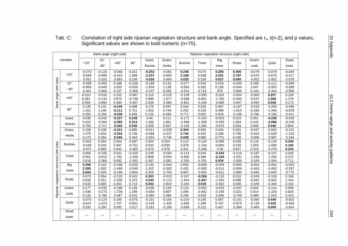
10 A
ppendix 10.2 H
ome range and activity patterns
244
Tab. C: Correlation of right side riparian vegetation structure and bank angle. Specified are rs, t(n-2), and p values.
Significant values are shown in bold numeric (n=75).
Bank angle (right side) Riparian vegetation structure (right side)
Variable <15°
15°
-45° >45° 90°
Sand,
Stones
Grass,
Herbs Bushes Trees
Big
trees Roots
Overh.
roots Quila
Dead
trees
<15° -0.070 -0.599 0.551
-0.116 -0.995 0.323
-0.048 -0.410 0.683
0.161 1.389 0.169
-0.253 -2.237 0.028
-0.081 -0.694 0.490
0.246 2.169 0.033
0.074 0.638 0.526
0.256 2.261 0.027
0.405 3.787 0.000
-0.079 -0.675 0.502
-0.079 -0.675 0.502
-0.049 -0.417 0.678
15°
- 45°
-0.098 -0.856 0.401
-0.052 -0.443 0.659
0.188 1.633 0.107
-0.108 -0.926 0.358
-0.188 -1.634 0.107
0.132 1.138 0.259
-0.077 -0.656 0.514
0.042 0.362 0.719
0.019 0.158 .875
-0.005 -0.044 0.965
0.189 1.647 0.104
-0.111 -0.952 0.344
-0.069 -0.588 0.559
>45° -0.010 -0.081 0.936
-0.016 -0.134 0.894
0.102 0.875 0.384
-0.087 -0.748 0.457
0.115 0.989 0.326
-0.125 -1.077 0.285
-0.109 -0.938 0.351
-0.093 -0.801 0.426
-0.202 -1.760 0.083
-0.054 -0.460 0.647
-0.063 -0.537 0.593
0.257 2.269 0.026
0.159 1.376 0.173
Ban
k an
gle
(left
side
)
90° 0.135 1.161 0.250
0.132 1.140 0.258
-0.240 -2.111 0.038
0.088 0.751 0.455
0.179 1.552 0.125
0.087 0.744 0.459
0.034 0.292 0.771
0.026 0.226 0.822
0.057 0.489 0.626
-0.187 -1.624 0.109
-0.033 -0.280 0.780
-0.256 -1.346 0.183
-0.096 -0.828 0.411
Sand,
Stones
0.036 0.313 0.755
-0.042 -0.364 0.717
-0.237 -2.095 0.040
0.249 2.213 0.030
0.46 1.266 0.209
0.211 1.861 0.067
-0.171 -1.496 0.139
-0.150 -1.308 0.195
-0.003 -0.030 0.976
0.223 1.964 0.053
0.051 0.443 0.659
-0.236 -2.086 0.040
-0.029 -0.249 0.804
Grass,
Herbs
0.158 1.375 0.173
0.108 0.933 0.354
-0.231 -2.044 0.045
0.085 0.736 0.464
-0.011 -0.096 0.924
-0.038 -0.327 0.745
0.304 2.744 0.008
0.005 0.042 0.966
0.034 0.289 0.773
0.091 0.785 0.435
-0.047 -0.402 0.689
-0.063 -0.545 0.587
-0.151 -1.310 0.194
Bushes -0.004 -0.036 0.972
0.050 0.434 0.665
0.054 0.467 0.642
-0.087 -0.751 0.455
0.004 0.033 0.973
-0.004 -0.030 0.976
0.113 0.978 0.331
-0.134 -1.164 0.248
-0.099 -0.860 0.39
0.026 0.220 0.827
0.116 1.003 0.319
-0.126 -1.090 0.279
0.244 2.162 0.034
Trees 0.058 0.501 0.618
-0.105 -0.910 0.366
0.201 1.763 0.082
-0.155 -1.348 0.182
0.105 0.908 0.367
-0.064 -0.554 0.581
-0.114 -0.990 0.326
0.044 0.380 0.705
-0.243 -2.160 0.034
-0.119 -1.031 0.306
-0.187 -1.636 0.106
-0.147 -1.283 0.204
0.043 0.372 0.711
Big
trees
0.259 2.305 0.024
0.116 1.002 0.320
-0.168 -1.468 0.146
-0.029 -0.249 0.804
0.133 1.152 0.253
-0.044 -0.382 0.703
0.050 0.432 0.667
-0.069 -0.593 0.555
-0.059 -0.511 0.611
-0.065 -0.556 0.580
-0.054 -0.463 0.645
-0.054 -0.463 0.645
-0.033 -0.287 0.775
Roots 0.073 0.626 0.533
0.064 0.551 0.583
-0.120 -1.039 0.302
0.043 0.370 0.713
0.353 3.244 0.002
-0.013 -0.113 0.910
-0.167 -1.454 0.150
-0.269 -2.407 0.019
-0.120 -1.040 0.302
0.010 0.089 0.930
-0.109 -0.942 0.349
-0.109 -0.942 0.349
0.166 1.444 0.153
Overh.
roots
0.177 1.548 0.126
-0.032 -0.273 0.786
-0.198 -1.736 0.087
0.139 1.208 0.231
-0.006 -0.050 0.960
0.100 0.867 0.389
0.123 1.065 0.290
-0.052 -0.452 0.653
-0.023 -0.195 0.846
-0.037 -0.321 0.749
0.002 0.014 0.989
-0.141 -1.226 0.224
0.059 0.824 0.413
Quila -0.075 -0.647 0.520
-0.124 -1.073 0.287
0.195 1.707 0.092
-0.075 -0.651 0.517
-0.151 -1.318 0.191
-0.164 -1.434 0.156
-0.210 -1.846 0.069
0.145 1.259 0.212
0.087 0.747 0.457
-0.101 -0.875 0.384
-0.084 -0.728 0.469
0.449 4.323 0.000
-0.052 -0.450 0.654
Rip
aria
n ve
geta
tion
stru
ctur
e (le
ft si
de)
Dead
trees --- --- --- --- --- --- --- --- --- --- --- --- ---

10 Appendix 10.3 Rearing cubs 245
10.3 Rearing cubs: effect on home range and activity pattern of a
female southern river otter (Lontra provocax Thomas 1908)
Tab. A: Calculated velocity of radio tracked southern river otter F 03/36 without and with cubs
Velocity (km/h) ID
x SE Maximum velocity
(km/h)
without cubs 1.47 0.09 10.64 with cubs 0.90 0.05 11.21 Average ( x ) 1.08 0.05 10.93
Tab B: Dens and resting sites used antenatal and postnatal without cubs
(April – June) with cubs
(Aug. – Sept.) with cubs
(Oct. – Nov.)
Dens and resting sites 10 (4)* 5 (3)* 14 (5)*
Distance from natal den to furthest den --- 3250 m 7813 m
* (x) = exclusively used in total time of radio-tracking
Tab. C: Hypothetical reproduction cycle of the southern river otter
Occurrence Duration Month Season
Period of conception 5 month Dec. – April Spring – Autumn
Gestation* variable delayed implantation
Dec. – July Spring – Winter
Birth --- July Autumn – Winter
Cub-rearing 7-8 month July – Feb. Winter – Spring
Travelling with mother 5 month Sept. – Feb. Winter – Summer
*= assumption

10 Appendix 10.4 Prey availability 246
10.4 Prey availability, diet composition and food competition
River bed structure
San
d
Gra
vel
Sto
nes
Roc
ks
Woo
dy d
ebris
Tree
s / R
oots
Aqu
atic
pla
nts
Inde
x
0,0
0,1
0,2
0,3
0,4
0,5
0,6
Simpson´s index of diversity (1-D)Smith & Wilson´s index of eveness (Evar)
(96) (71) (28) (8) (1014) (112) (688)
Fig. A: Evenness and species diversity of all electrofished sites
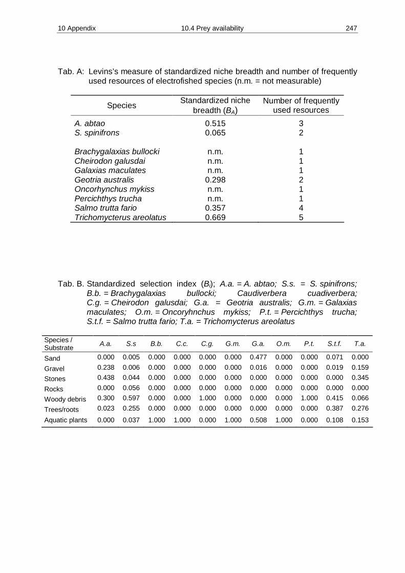
10 Appendix 10.4 Prey availability 247
Tab. A: Levins’s measure of standardized niche breadth and number of frequently
used resources of electrofished species (n.m. = not measurable)
Species Standardized niche breadth (BA)
Number of frequently used resources
A. abtao 0.515 3 S. spinifrons 0.065 2 Brachygalaxias bullocki n.m. 1 Cheirodon galusdai n.m. 1 Galaxias maculates n.m. 1 Geotria australis 0.298 2 Oncorhynchus mykiss n.m. 1 Percichthys trucha n.m. 1 Salmo trutta fario 0.357 4 Trichomycterus areolatus 0.669 5
Tab. B. Standardized selection index (Bi); A.a. = A. abtao; S.s. = S. spinifrons; B.b. = Brachygalaxias bullocki; Caudiverbera cuadiverbera; C.g. = Cheirodon galusdai; G.a. = Geotria australis; G.m. = Galaxias maculates; O.m. = Oncoryhnchus mykiss; P.t. = Percichthys trucha; S.t.f. = Salmo trutta fario; T.a. = Trichomycterus areolatus
Species / Substrate A.a. S.s B.b. C.c. C.g. G.m. G.a. O.m. P.t. S.t.f. T.a.
Sand 0.000 0.005 0.000 0.000 0.000 0.000 0.477 0.000 0.000 0.071 0.000
Gravel 0.238 0.006 0.000 0.000 0.000 0.000 0.016 0.000 0.000 0.019 0.159
Stones 0.438 0.044 0.000 0.000 0.000 0.000 0.000 0.000 0.000 0.000 0.345
Rocks 0.000 0.056 0.000 0.000 0.000 0.000 0.000 0.000 0.000 0.000 0.000
Woody debris 0.300 0.597 0.000 0.000 1.000 0.000 0.000 0.000 1.000 0.415 0.066
Trees/roots 0.023 0.255 0.000 0.000 0.000 0.000 0.000 0.000 0.000 0.387 0.276
Aquatic plants 0.000 0.037 1.000 1.000 0.000 1.000 0.508 1.000 0.000 0.108 0.153

10 A
ppendix 10.4 P
rey availability 248
Tab. C: River bed characteristics, species density and presence of eleven electrofished sites (2003)
Section Substrate Type in m3 Number of captures a
Sand Gravel Stones Rocks Woody debris
Trees / Roots
Aquatic plants A.a. S.s. B.b. C.c. C.g. G.m. G.a. O.m. P.t. S.t.f. T.a.
Q 01 17 33 20 0 30 0 0 3 96 0 0 0 0 12 0 0 3 0
Q 02 10 50 3 5 32 0 0 67 133 0 0 0 0 7 0 0 2 1
Q 03 100 0 0 0 0 0 0 0 1 0 0 0 0 17 0 0 0 0
Q 04 10 27 0 16 47 0 0 8 147 0 0 0 0 6 0 2 2 1
Q 05 63 33 0 0 4 0 0 11 168 0 0 0 0 16 0 0 3 0
Q 06 56 17 17 0 10 0 0 12 60 0 0 0 0 3 0 0 1 1
Q 07 0 83 0 0 17 0 0 12 54 0 0 0 0 10 0 1 4 0
Q 08 35 42 0 0 23 0 0 8 300 0 0 1 0 9 0 1 9 2
Q 09 60 0 0 0 20 20 0 1 78 0 0 1 0 0 0 0 4 1
Q 10 20 0 0 0 40 40 0 1 49 0 0 0 0 0 0 0 0 0
M 01 0 0 0 0 5 0 95 0 24 20 2 2 615 22 2 0 2 1
Total 371 285 40 21 228 60 95 123 1110 20 2 4 615 102 2 4 30 7
Presence 81.8 63.6 27.3 18.2 90.1 18.1 9.1 81.8 100 9.1 9.1 27.3 9.1 81.8 9.1 27.3 81.8 54.5
Q = Upper Queule River M = Mahuidanche River a Species: A. abtao, S. spinifrons, Brachygalaxias bullocki, Caudiverbera caudiverbera, Cheirodon galusdai, Galaxias maculates,
Geotria australis, Oncorhynchus mykiss, Percichthys trucha, Salmo trutta fario, Trichomycterus areolatus
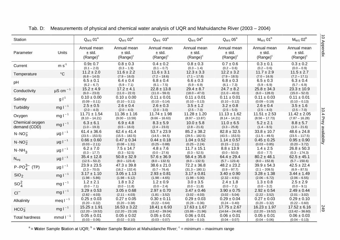
10 A
ppendix 10.4 P
rey availability 249
Tab. D: Measurements of physical and chemical water analysis of UQR and Mahuidanche River (2003 – 2004)
Station QWS 01a QWS 02a QWS 03a QWS 04a QWS 05a MWS 01b MWS 02b
Parameter Units Annual mean
± std. (Range)c
Annual mean ± std.
(Range)c
Annual mean ± std.
(Range)c
Annual mean ± std.
(Range)c
Annual mean ± std.
(Range)c
Annual mean ± std.
(Range)c
Annual mean ± std.
(Range)c
Current m s-1 0.9± 0.7 (0.1 – 2.0)
0.8 ± 0.3 (0.3 – 1.9)
0.4 ± 0.2 (0.1 – 0.7)
0.8 ± 0.3 (0.3 – 1.4)
0.7 ± 0.6 (0.2 – 0.6)
0.3 ± 0.1 (0.2 – 0.6)
0.3 ± 0.2 (0.0 – 0.9)
Temperature °C 11.2 ± 2.0 (6.8 – 14.0)
11.6 ± 2.2 (7.9 – 16.0)
11.6 ± 3.1 (7.2 – 18.6)
12.3 ± 3.3 (7.1 – 17.8)
12.2 ± 3.2 (7.9 – 18.5)
11.7 ± 2.9 (7.0 – 16.9)
11.5 ± 2.7 (7.2 – 17.1)
pH 6.5 ± 0.1 (6.2 – 6.7)
6.4 ± 0.4 (5.9 – 7.1)
6.8 ± 0.4 (6.1 – 7.5)
6.6 ± 0.3 (5.9 – 6.9)
6.8 ± 0.3 (6.1 – 7.3)
6.5 ± 0.3 (5.9 – 6.9)
6.3 ± 0.4 (5.7 – 6.9)
Conductivity µS cm – 1 15.2 ± 4.9 (6.0 – 23.0)
17.2 ± 4.1 (11.0 – 22.0)
22.8 ± 13.8 (11.0 – 59.0)
29.4 ± 8.7 (18.0 – 47.0)
24.7 ± 8.2 (11.0 – 43.0)
25.8 ± 34.3 (6.0 – 128.0)
23.3 ± 10.9 (15.0 – 52.0)
Salinity g l-1 0.10 ± 0.00 (0.09 – 0.11)
0.10 ± 0.00 (0.10 – 0.11)
0.11 ± 0.01 (0.10 – 0.14)
0.11 ± 0.01 (0.10 – 0.13)
0.11 ± 0.01 (0.10 – 0.12)
0.11 ± 0.03 (0.09 – 0.19)
0.11 ± 0.01 (0.10 – 0.13)
Turbidity mg l – 1 2.5 ± 0.5 (2.0 – 4.0)
2.6 ± 0.4 (2.0 – 4.0)
2.6 ± 0.3 (2.0 – 3.0)
3.5 ± 1.2 (2.5 – 7.0)
3.2 ± 0.8 (2.5 – 5.0)
2.6 ± 0.4 (2.5 – 4.0)
3.5 ± 1.6 (2.5 – 7.0)
Oxygen mg l – 1 11.71 ± 1.54 (8.10 – 14.21)
11.36 ± 1.16 (9.00 – 13.59)
11.74 ± 1.98 (9.66 – 16.63)
11.28 ± 1.20 (8.97 – 13.87)
11.13 ± 1.62 (8.14 – 14.21)
11.51 ± 2.53 (8.56 – 17.73)
11.42 ± 2.05 (7.87 – 16.28)
Chemical oxygen demand (COD) mg l – 1 6.3 ± 6.1
(1.0 – 19.3) 6.9 ± 4.8 (0.5 – 16.0)
8.3 ± 5.9 (2.4 – 23.0)
10.0 ± 5.8 (2.8 – 21.6)
11.0 ± 6.5 (3.3 – 25.8)
5.2 ± 2.1 (1.4 – 8.5)
8.8 ± 5.7 (1.0 – 21.6)
–3NO-N µg l – 1 61.4 ± 36.6
(23.5 – 153.5) 62.4 ± 41.4 (15.5 – 182.5)
53.7 ± 23.9 (14.5 – 94.5)
85.2 ± 38.2 (29.5 – 182.5)
82.8 ± 32.5 (43.5 – 153.5)
33.8 ± 10.7 (11.5 – 49.5)
48.6 ± 24.8 (23.5 – 117.5)
–2NO-N µg l – 1 0.66 ± 0.60
(0.03 – 2.11) 0.47 ± 0.34 (0.08 – 1.31)
0.44 ± 0.18 (0.25 – 0.88)
1.04 ± 0.52 (0.25 – 2.24)
1.14 ± 0.57 (0.15 – 2.11)
0.45 ± 0.25 (0.03 – 0.85)
0.95 ± 0.90 (0.20 – 3.72)
+3NH-N µg l – 1 6.2 ± 7.0
(0.3 – 17.7) 7.5 ± 14.7 (0.3 – 52.5)
4.8 ± 7.6 (0.0 – 27.6)
11.7 ± 15.1 (0.3 – 52.5)
8.8 ± 13.9 (0.0 – 50.0)
1.4 ± 2.5 (0.0 – 7.7)
26.8 ± 50.3 (0.3 – 174.3)
Norg µg l – 1 35.4 ± 12.8 (12.5 – 53.2)
50.8 ± 32.9 (8.0 – 123.4)
57.6 ± 36.9 (8.0 – 132.5)
58.4 ± 35.8 (8.0 – 132.5)
64.4 ± 29.4 (5.7 – 123.4)
80.2 ± 48.1 (8.0 – 152.8)
62.5 ± 45.1 (5.7 – 150.6)
–34PO-P (TP) µg l – 1 23.9 ± 23.5
(2.3 – 70.0) 47.3 ± 39.8 (16.2 – 132.4)
38.6 ± 21.0 (0.7 – 76.4)
72.2 ± 36.8 (31.3 – 180.1)
48.2 ± 23.2 (0.9 – 97.7)
39.9 ± 54.3 (2.1 – 209.5)
42.5 ± 22.4 (6.9 – 87.5)
2SiO mg l – 1 3.17 ± 1.10 (1.98 – 5.86)
3.05 ± 1.13 (1.98 – 6.12)
2.93 ± 0.81 (1.98 – 4.65)
3.17 ± 0.81 (1.98 – 5.00)
3.40 ± 0.90 (2.32 – 4.91)
3.28 ± 1.38 (2.06 – 6.72)
3.44 ± 1.49 (2.06 – 6.55)
+24SO mg l – 1 1.2 ± 2.1
(0.0 – 7.1) 1.8 ± 3.2 (0.0 – 11.8)
1.2 ± 0.9 (0.0 – 2.4)
3.0 ± 3.5 (0.0 – 11.8)
2.4 ± 1.8 (0.0 – 7.1)
1.3 ± 0.8 (0.0 – 3.2)
2.5 ± 2.9 (0.0 – 9.1)
–Cl mg l – 1 3.29 ± 0.53 (2.82 – 4.03)
3.05 ± 0.68 (2.11 – 4.03)
2.97 ± 0.70 (1.81 – 3.52)
3.47 ± 0.46 (3.02 – 4.03)
3.90 ± 0.75 (3.02 – 5.04)
2.92 ± 0.54 (2.22 – 3.52)
2.49 ± 0.44 (2.01 – 3.02)
Alkalinity meq l – 1 0.25 ± 0.03 (0.20 – 0.32)
0.27 ± 0.05 (0.20 – 0.38)
0.30 ± 0.11 (0.22 – 0.64)
0.29 ± 0.03 (0.26 – 0.36)
0.29 ± 0.04 (0.24 – 0.40)
0.27 ± 0.03 (0.20 – 0.32)
0.29 ± 0.10 (0.22 – 0.60)
–3HCO mg l – 1 15.25 ± 1.91
(12.20 – 19.52) 16.53 ± 3.22 (12.20 – 23.18)
18.41 ± 6.93 (13.42 – 39.04)
17.63 ± 1.67 (15.86 – 21.96)
17.75 ± 2.67 (14.64 – 24.40)
16.23 ± 1.97 (12.20 – 19.52)
17.52 ± 6.16 (13.42 – 36.60)
Total hardness mmol l – 1 0.05 ± 0.01 (0.03 – 0.06)
0.05 ± 0.02 (0.02 – 0.10)
0.05 ± 0.01 (0.03 – 0.07)
0.06 ± 0.01 (0.04 – 0.10)
0.06 ± 0.01 (0.04 – 0.07)
0.05 ± 0.01 (0.04 – 0.06)
0.06 ± 0.03 (0.04 – 0.13)
a = Water Sample Station at UQR; b = Water Sample Station at Mahuidanche River; c = minimum – maximum range

10 Appendix 10.4 Prey availability 250
Tab. E: Energy content (Kcal/100g) of crustacean and fish
Species Kcal/100g Crustacean Samastacus spinifrons 99 Aegla abtao 88 Fish Salmo trutta fario 157 Odontesthes regia 125

10 Appendix 10.5 Age determination 251
10.5 Age determination of male southern river otter Lontra
provocax (Thomas 1908)
Tab. A: Measurements of dental pulp
Animal max. pulp width in mm
max. dental width in mm
relative width in %
M 04/x2 5.17 7.75 66.70 M 04/x1 1.92 7.75 24.80 M 03/x1 1.44 7.94 18.10 M 01/06 1.03 8.07 12.80
Fig. A: Skull of M 04/x2:
1 = transverse palatine suture (Sutura palatina transversa) 2 = speno-occipital synchondrosis (Synchondrosis spheno-occipitalis)
1 2
A

10 Appendix 10.5 Age determination 252
Fig. B: Skull of M 04/x2:
3 = naso-maxillary suture (Sutura nasomaxillaris) 4 = frontonasal suture (Sutura frontnasalis) 5 = coronal suture (Sutura coronalis) 6 = sagittal suture (Sutura sagittalis)
Fig. C: Skull of M 04/x2: 7 = frontozygomaic suture (Sutura frontozygomatica) 8 = maxillozygomatic suture (Sutura zygomaticomaxillaris) 9 = zygomatico-temporal suture (Sutura temporozygomatica) 10 = squamomastoid suture (Sutura squamosomastoidea)
4 6 5
3
B
7
8 9 10
C

CURRICULUM VITAE
Name: Renato Luis-Goetz Reyes Küppers Date of Birth: March 2nd, 1969 Birthplace: Germersheim, Rhineland-Palatinate, Germany Marital Status: Married Children: 1 son, Pepe Reyes Küppers (27.12.2000) Nationality: German Qualifications: PhD student (since April 2002)
University of Osnabrück / Germany Topic of thesis: ”Ecology and Behaviour of the Southern River Otter
Lontra provocax THOMAS 1908 in Chile”
MSc (May 2000) Topic of thesis: “Establishing of a non-invasive method to determine the
reproductive status of the Giant Jumping Rat, Hypogeomys antimena (Rodentia, Nesomyinae)”
Studies of Biology
Zoology (Ecology), Hydrobiology and Fisheries Science, Nature Conservation University of Hamburg / Germany (October 1993 – May 2000)
A-level (1990) Ernst-Barlach-Gymnasium
Unna / Germany
Languages:
German (native), English (advanced), Spanish (intermediate)
Military Service: Regular soldier, corpsman Hamburg / Germany (July 1990 – June 1992)
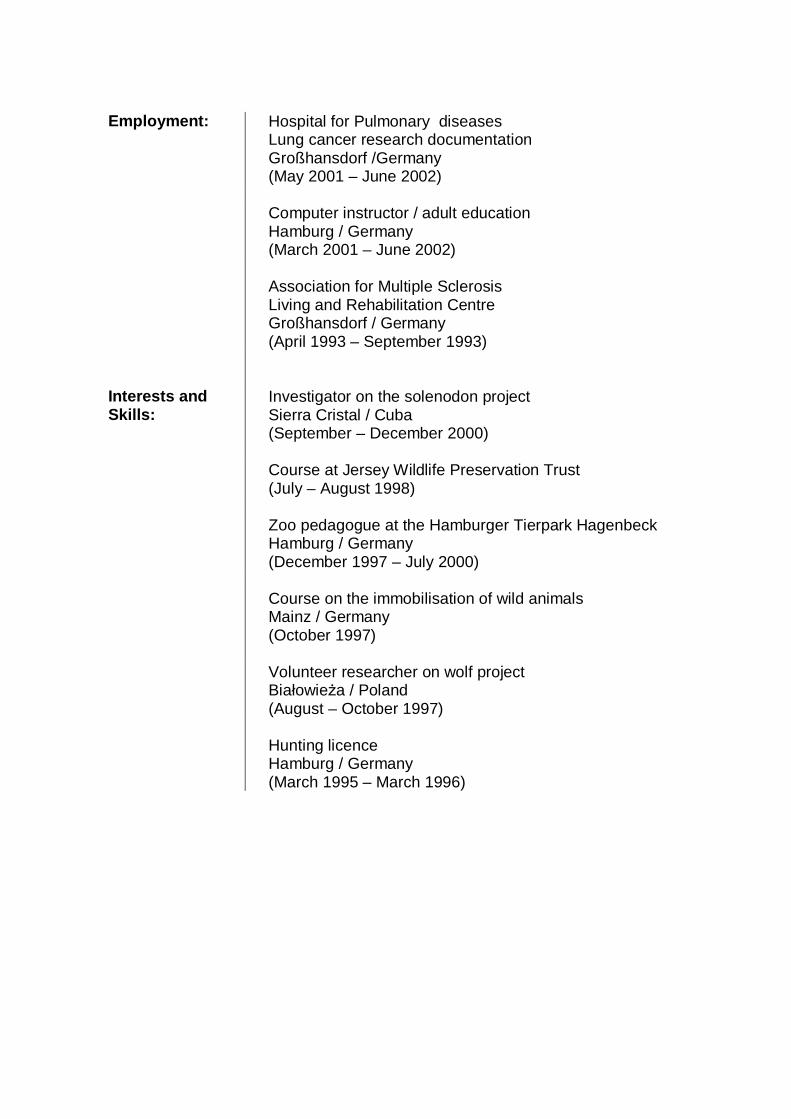
Employment: Hospital for Pulmonary diseases
Lung cancer research documentation Großhansdorf /Germany (May 2001 – June 2002)
Computer instructor / adult education
Hamburg / Germany (March 2001 – June 2002)
Association for Multiple Sclerosis
Living and Rehabilitation Centre Großhansdorf / Germany (April 1993 – September 1993)
Interests and Skills:
Investigator on the solenodon project Sierra Cristal / Cuba (September – December 2000)
Course at Jersey Wildlife Preservation Trust
(July – August 1998) Zoo pedagogue at the Hamburger Tierpark Hagenbeck
Hamburg / Germany (December 1997 – July 2000)
Course on the immobilisation of wild animals
Mainz / Germany (October 1997)
Volunteer researcher on wolf project
Białowieża / Poland (August – October 1997)
Hunting licence
Hamburg / Germany (March 1995 – March 1996)