Embed Size (px)
Citation preview

Ecological, Evolutionary, and Taphonomic Comparisons of Brachiopods and Bivalves at Multiple Spatial and Temporal Scales
Richard Alan Krause Jr.
Dissertation submitted to the faculty of the Virginia Polytechnic Institute and State University in partial fulfillment of the requirements for the degree of
Doctor of Philosophy
In Department of Geosciences
Michał Kowalewski (Chair) Arnold I. Miller
J. Fred Read Stephen E. Scheckler
Shuhai Xiao
14 April 2006 Blacksburg, Virginia
Keywords: bivalve, brachiopod, time averaging, morphometrics; size
ii
Ecological, Evolutionary, and Taphonomic Comparisons of Brachiopods and Bivalves at Multiple Spatial and Temporal Scales
Richard A. Krause Jr.
Abstract
The fossil record is the primary source of information on the history of life. As such, it is important to understand the limitations of this record. One critical area in which there is still much work to be done is in understanding how the fossil record, and our interpretation of it, may be biased.
Herein, the fidelity between the life and death assemblage of an extant brachiopod with respect to morphological variability is studied using geometric morphometrics. The results from several analyses confirm a high degree of morphological variability with little change in mean shape between the living and sub-fossil assemblage. Additionally, there is no evidence of distinct morphogroups in either assemblage. These trends persist at all depths and size classes indicating that this species could be recognized as a single, rather than multiple, species if only fossil data were available.
The second chapter involves the recognition and quantification of a worker bias in monographs of brachiopods and bivalves. Most specimens studied came from the 65th to 69th percentile of their species’ bulk-collected size-frequency distribution. This indicates a significant bias toward monograph specimens that are larger than the mean size of the bulk sample. When compared at the species level, this bias was found to be highly consistent among the 86 species included in the study. Thus, size measurements of monographed specimens reliably and consistently record a similar size class for any given species, and this bias is easily corrected during meta-analyses.
Chapter three focuses on bivalves and brachiopods from a modern tropical shelf and quantifies the magnitude of time averaging (temporal mixing) for these two different organisms. This is accomplished by dating a suite of shells from each site using amino acid racemization calibrated with several radiocarbon dates. By studying the age distributions for each species it is determined that, despite some site to site differences, both bivalve and brachiopod species exhibit a similar time averaging magnitude when collected from the same region or depositional system. This indicates that fossil assemblages of these species may have very similar resolution.
iii
TABLE OF CONTENTS
TABLE OF CONTENTS........................................................................................................................................ III LIST OF FIGURES.................................................................................................................................................. V LIST OF TABLES .................................................................................................................................................. VI INTRODUCTION AND OVERVIEW OF THE RESEARCH.............................................................................. VII ATTRIBUTION...................................................................................................................................................... XI ACKNOWLEDGEMENTS................................................................................................................................... XII
CHAPTER ONE: AN ASSESSMENT OF MORPHOLOGICAL FIDELITY IN THE SUB-FOSSIL RECORD OF A TEREBRATULIDE BRACHIOPOD............................................................................................1
ABSTRACT .............................................................................................................................................................2 INTRODUCTION ....................................................................................................................................................3
Previous Work......................................................................................................................................................4 MATERIAL AND METHODS ................................................................................................................................6
Sample Collection ................................................................................................................................................6 Data Collection ....................................................................................................................................................8 Analytical Methods ..............................................................................................................................................9
Procrustes Analysis........................................................................................................................................................... 9 Comparison of fitting techniques .................................................................................................................................... 10 Operator Error Estimation............................................................................................................................................... 10 Principal Components Analysis ...................................................................................................................................... 11 Canonical Variates Analysis ........................................................................................................................................... 11 Thin-Plate Spline Analysis.............................................................................................................................................. 14 Variability Metrics .......................................................................................................................................................... 15
RESULTS AND DISCUSSION .............................................................................................................................20 Mean Shape vs. Mean Variability ......................................................................................................................20 Live-Dead Comparisons ....................................................................................................................................20
Results............................................................................................................................................................................. 20 Discussion....................................................................................................................................................................... 21
Depth Comparisons............................................................................................................................................24 Results............................................................................................................................................................................. 24 Discussion....................................................................................................................................................................... 27
Size Comparisons...............................................................................................................................................27 Results............................................................................................................................................................................. 27 Discussion....................................................................................................................................................................... 30
CONCLUSIONS ....................................................................................................................................................32 CHAPTER TWO: BODY SIZE ESTIMATES FROM THE LITERATURE: UTILITY AND POTENTIAL FOR MACROEVOLUTIONARY STUDIES .........................................................................................................33
ABSTRACT ...........................................................................................................................................................34 INTRODUCTION ..................................................................................................................................................35 TYPES OF PHOTOGRAPHIC BIAS.....................................................................................................................37
Apparent Versus Actual Size ..............................................................................................................................37 Sampling Bias ....................................................................................................................................................37
METHODS.............................................................................................................................................................39 Specimen-Level Analysis....................................................................................................................................40 Species-Level Analysis .......................................................................................................................................40
RESULTS...............................................................................................................................................................43 Specimen-Level Analysis....................................................................................................................................43 Species-Level Analysis .......................................................................................................................................43 Confounding Factors .........................................................................................................................................45
Country of Publication .................................................................................................................................................... 45 Year of Publication ......................................................................................................................................................... 45 Sample Size..................................................................................................................................................................... 46
DISCUSSION.........................................................................................................................................................50 Characterization of the Bias ..............................................................................................................................50

iv
An Additional Confounding Factor....................................................................................................................53 Implications........................................................................................................................................................53
CONCLUSIONS ....................................................................................................................................................55 CHAPTER THREE: COMPARATIVE TIME AVERAGING: AGE MIXING AMONG SYMPATRIC BIVALVES AND BRACHIOPODS FROM A MODERN TROPICAL SHELF.................................................56
ABSTRACT ...............................................................................................................................................................57 INTRODUCTION ........................................................................................................................................................59 BACKGROUND .........................................................................................................................................................61
Study Area..........................................................................................................................................................61 Bouchardia rosea...............................................................................................................................................61 Semele casali......................................................................................................................................................62 Dating Technique...............................................................................................................................................63
MATERIALS AND METHODS.....................................................................................................................................64 Sample Collection ..............................................................................................................................................64 Amino Acid Racemization Dating ......................................................................................................................64 Quantification and Comparison of Time Averaging ..........................................................................................66 Completeness Analysis .......................................................................................................................................68
RESULTS..................................................................................................................................................................71 Magnitude and Variation of Time Averaging.....................................................................................................71 Age Structure and Completeness .......................................................................................................................72
DISCUSSION AND IMPLICATIONS..............................................................................................................................76 Comparisons Between the Two Species and Sites..............................................................................................76 Comparisons with other regions ........................................................................................................................78
CONCLUSIONS .........................................................................................................................................................81 REFERENCES .......................................................................................................................................................82 APPENDICES ........................................................................................................................................................95
Appendix 1.1: Raw landmark coordinates – Anterior view ...............................................................................95 Appendix 1.2: Raw Landmark coordinates – Dorsal view.................................................................................99 Appendix 2.1: Bulk Sample raw data ...............................................................................................................103 Appendix 2.2: Monograph raw data ................................................................................................................114 Appendix 3.1: Amino Acid Ratios and Dates ...................................................................................................130 Appendix 3.2: Bootstrap program for SAS/IML...............................................................................................133 Appendix 3.3: Completeness simulation in SAS...............................................................................................135

v
LIST OF FIGURES
1.1 San Juan Islands locality 6 1.2 Landmark locations 8 1.3 Comparison of fitting techniques 11 1.4 Operator error estimation 12 1.5 Principle components analysis: anterior view 13 1.6 Principle components analysis: dorsal view 14 1.7 Canonical variates analysis 15 1.8 Live-dead comparisons 19 1.9 Allometry-free variability comparisons 22 1.10 Superimposition plots: anterior – depth groups 25 1.11 Superimposition plots: dorsal – depth groups 26 1.12 Superimposition plots: anterior live/dead – depth groups 27 1.13 Superimposition plots: dorsal live/dead – depth groups 28 1.14 Comparison of centroid sizes 29 1.15 Superimposition plots: size groups 30 1.16 Superimposition plots: anterior live/dead – size groups 31 1.17 Superimposition plots: dorsal live/dead – size groups 31 2.1 Construction of the datasets 41 2.2 Null models for species-level analysis 42 2.3 Percentile-frequency distributions 43 2.4 Descriptive statistics of percentile-frequency distributions 43 2.5 Species-level analysis scatterplots 47 2.6 Percentile-frequency distributions: regional groups 48 2.7 Descriptive statistics: regional groups 48 2.8 Species-level analysis scatterplots: regional groups 49 2.9 Percentile-frequency distributions: year of publication 49 2.10 Descriptive statistics: year of publication 50 2.11 Species-level analysis scatterplots: year of publication 50 2.12 Percentile-frequency distributions: sample size 51 2.13 Percent difference plots 52 2.14 Monograph vs. bulk sample comparisons 54 3.1 Ubatuba Bay locality 64 3.2 Age-frequency distributions 70 3.3 Semi-quartile range comparisons 72 3.4 Maximum age vs. rate parameter 74 3.5 Completeness simulations 75 3.6 Semi-quartile range vs. depth 80

vi
LIST OF TABLES 1.1 Depth distribution of samples 7 1.2 Landmark descriptions 9 1.3 Variability values for replicate samples 12 1.4 Variability values 17 1.5 Mahalanobis distances derived from CVA 18 2.1 Monograph and bulk sample descriptions 38 2.2 Basic statistics for percentile distributions 44 2.3 Percentile distribution comparisons 45 2.4 Species-level regressions 46 2.5 Percentile distribution comparisons: other groups 48 3.1 Sediment characteristics for the collections sites 62 3.2 Descriptive statistics 67 3.3 Completeness simulations 69

vii
INTRODUCTION AND OVERVIEW OF THE RESEARCH
As one of the primary sources of information on the history of life, the fossil record is an
important resource for anyone trying to understand the patterns and processes of evolution.
During the past several centuries, intensive study of the fossil record has led to many important
breakthroughs that have greatly increased our knowledge of how life on earth began and how it
has prospered. Despite these insights, there is still much that we do not know.
One critical area in which there is still much work to be done is in understanding how the
fossil record may be biased. Biases in the fossil record can take many forms, and the study of
most of these biases can be grouped under the heading of Taphonomy. Taphonomy is literally
the science of the “laws of burial” (from the Greek taphos + nomos), and was practiced long
before the term was first coined by Efremov (1940). In fact, some of the first taphonomic
investigations were conducted by Leonardo da Vinci, who used observations on living and dead
bivalves to infer that fossils found in nearby mountains had not been transported there by the
Biblical Deluge, but rather had lived and died in situ (Martin 1999). As the science of
taphonomy has emerged as a distinct entity over the last two decades, it’s principles have been
applied rather broadly to the fossil record, and its definition has solidified as “the study of the
processes of preservation and how they affect information in the fossil record” (Behrensmeyer
and Kidwell 1985). Some general principles of taphonomy that have been outlined by Wilson
(1988), and modified by Martin (1999) are as follows:
1. Organisms are more likely to be preserved if they have hardparts.
2. Preservation is greatly enhanced by rapid burial, especially in fine-grained sediment and/or in the absence of
decay and scavenging. Rapidly buried deposits can serve as ecological “snapshots” of the living community.
3. During the transition from a living assemblage of organsisms to an assemblage of the remains of dead
organisms, disarticulation and chemical alteration resulting from decay, abrasion, transporation, predation,
scavenging, or dissolution can cause the loss of information about species abundances and community
diversity and structure. This information loss is typically most severe in shallow-water marine depositional
systems.
4. Fossil assemblages typically consist of spatially-averaged remains. That is, a fossil assemblage can consist of
organisms that have been preserved in life position, organisms that have been disarticulated, reoriented, or
concentrated from the original position by bioturbators, predators, or scavengers, but have not been
transported out of their original community, and foreign remains that have been derived from other
communities.
viii
5. Bioturbation and physical reworking can also cause fossil assemblages to become time averaged (temporally
mixed) and this may lead to increased diversity and morphological variation within and assemblage.
Of course, each of the points listed above represent types of bias in the fossil record, and
they can greatly affect how data from a fossiliferous deposit are interpreted. As the science of
taphonomy has matured, and the body of theory behind these principles has grown, it has
become possible to begin predicting the utility of the fossil record for various types of
evolutionary or paleoecological questions (Martin 1999). For example, it is now generally
appreciated that studies of the ecological aspects of a fossil assemblage, such as population
dynamics, should only be done on assemblages that were rapidly buried thereby minimizing the
temporal and spatial mixing that could lead to incorrect interpretations. In this way, and many
others, paleontologists have begun using their knowledge of the biases imposed on the fossil
record by taphonomic processes to interpret the history of the formation of fossil assemblages.
In addition to the biases that can be grouped under the heading of taphonomy, there is
another set of biases that can greatly affect the quality of the information that can be obtained
from the fossil record. This second group of biases can be broadly grouped under the heading of
woker biases, or biases due to sampling, processing, or analysis of data from the fossil record.
While this type of bias is certainly not unique to paleontology, it has, nevertheless, become an
active area of paleontological research in the last several decades. Through research on worker
bias, it has been appreciated that the apparent patterns in the fossil record may be reflective of
nothing more than where paleontologists choose to look (Sheehan 1977), or where and from
what time periods rocks are preserved (Raup 1976; Peters and Foote 2001). Developing a better
understanding of these types of biases can give paleontologists insight into the veracity of the
patterns that are seen in the fossil record.
This dissertation focuses on both of types of bias listed above. Specifically, in the
chapters that follow, several specific biases and their implications for the fossil record will be
discussed. Each of the three chapters focus on the fossil records of bivalves and brachiopods and
in two of three chapters, the fossil records of these two common marine organisms will be
compared to gain additional insight into the quality of the record.
In chapter one, the deleterious effects of time averaging are explored in the sub-fossil
record of an extant brachiopod species. Specifically, this chapter focuses on the recognition of
morphological variability in the fossil record, and the fidelity between the life and death

ix
assemblage with respect to this parameter. To explore this issue, several geometric
morphometric techniques are employed that enable quantification and direct comparison of
morphology between different populations. The fidelity of the fossil record, used here to refer to
how closely, or accurately, the fossil record captures original biological information
(Behrensmeyer et al., 2000), is a branch of research on time-averaging that has been particularly
successful, but has been under-investigated. The brachiopod that is the focal point of chapter
one, Terebratalia transversa is extremely morphologically variable in all known living
populations and this research was undertaken to determine if this high degree of variability could
be recognized in the fossil record of this species.
The results from several geometric morphometric techniques (including procrustes
analysis and thin-plate spline) confirm a high degree of morphological variability with little
change in mean shape between the living and sub-fossil assemblage. Additionally, there is no
evidence of distinct morphogroups in either assemblage, as postulated for the species in previous
studies (Schuman 1990). These trends persist at all depths and size classes. The similar range of
morphological variability at each site suggests a common causal factor such as a similar array of
micro-environments available at all depths. Another implication of this consistency between the
living and the dead assemblage is that the variability of a fossil assemblage of this species could
be used to estimate single-generation variability during the time averaged interval. Finally, it is
encouraging to note that, given the full range of morphological variability in the fossil record of
this brachiopod, this species could be recognized as a single, rather than multiple, species if only
fossil data were available.
The second chapter involves the recognition and quantification of an underappreciated
worker bias in the published literature on brachiopods and bivalves. This bias involves the
images of specimens that are published in descriptions of species or faunas. Such images are an
important and relatively untapped resource for paleontologists. Among other things they can
provide a vast of amount of data on body size evolution to the researcher that takes simple
measurements of the images. However, before images in the published literature can be used in
this manner, any difference in the average size between photographed specimens and the
populations from which these specimens were drawn must be evaluated and quantified. This is
the focal point of chapter two. Specifically, the quality of data from published images is
assessed therin with respect to three parameters: (1) bias direction – the presence of non-random
departures from the actual mean size of a species; (2) bias magnitude – the absolute value of the
x
mean departure, that is, the imprecision of the data; and (3) bias consistency – the variation in the
direction and magnitude of bias within and across monographs, higher taxa, or time intervals.
With a clear understanding of these bias parameters it is possible to assess the utility of
monograph-derived size data.
Finally, chapter three is a comparative study of assemblages of sympatric Holocene
bivalves and brachiopods from a modern tropical shelf (Southeast Brazilian Bight, South
Atlantic). This study is one of the first to quantify the magnitude of time averaging (the amount
of temporal mixing) for two different organisms collected from the same sites. Quantification of
time averaging is accomplished by dating a suite of shells from each site using amino acid
racemization calibrated with several AMS radiocarbon dates. By studying the age distributions
for each species at each site it is determined that, despite some site to site differences, both
bivalve and brachiopod species exhibit a very similar time averaging magnitude when collected
from the same region and/or depositional system. Furthermore, by comparing the data described
in chapter three with other previously published data of the same type, but from different depths
and depositional systems, a significant correlation between depth and duration of time averaging
is noted. This finding provides a basis for the third general principle of taphonomy (mentioned
above) that shallow water skeletal assemblages are more susceptible to the processes of
taphonomic destruction than are deeper water assemblages. This translates into a greater time
averaging magnitude for deeper water assemblages because skeletal elements can survive longer
in these environments. The most striking thing about this pattern is that it is very similar for
vastly different depositional environments and latitudes, indicating that a wide array of skeletal
assemblages may follow this pattern of increasing time averaging magnitude with increasing
depth.

xi
ATTRIBUTION
Each of the following chapters has been prepared with the goal of eventual publication in
peer-reviewed journals. Chapter one has already been published (Krause 2004), chapter two was
submitted in November of 2005, and chapter three will be submitted in May of 2006.
Chapter one is published as a single-authored work. As such, 100% of the work behind
chapter one was done by R. A. Krause. Chapters two and three, when published, will be
published as multiple authored papers because these studies represent portions of ongoing
collaborative studies. However, the coauthors for these papers (listed on the title page for each
chapter) contributed less than 20% to the data collection, analysis, and writing for these papers.
As a result, these chapters can be considered to be mostly the work of R. A. Krause, which
justifies their inclusion in this dissertation.
xii
ACKNOWLEDGEMENTS
Field work for chapter one was conducted while participating in a course in Invertebrate
Taphonomy during summer, 2002 at Friday Harbor Laboratories of the University of
Washington. The organizers of the course, M. Kowalewski and M. LaBarbera, and the T.A., T.
Rothfus, offered countless hours of help and support, without which this project could not have
been completed. The faculty and staff of Friday Harbor Laboratories also provided invaluable
financial and technical support, especially C. Staude, captain of the R/V Nugget during sampling
voyages. The detailed peer reviews of M. Sandy and two anonymous reviewers greatly
improved the structure and methodology of the study.
For assistance with the second chapter, I would like to thank John Alroy, Colin Sumrall,
and Steve Wang for helpful discussions. John Pojeta and Lauck Ward provided hospitality and
logistical support during research visits to the National Museum of Natural History and the
Virginia Museum of Natural History, respectively. Susan Barbour-Wood helped with some of
the data collection. Generous financial support was provided by the Paleobiology Database and
the Department of Geosciences at Virginia Tech.
The third chapter benefited from discussions with M. Carroll and D. Rodland. I also
thank M. Carroll for allowing access to her data. This project was funded by National Science
Foundation grants, EAR0125149 (Kowalewski) and EAR124767 (Goodfriend [then
Wehmiller]), and by a Research Grant from the Petroleum Research Fund of the American
Chemical Society (AC-PRF#40735-AC2) to Kowalewski.

1
CHAPTER ONE1: An Assessment of Morphological Fidelity in the
Sub-fossil Record of a Terebratulide Brachiopod
1 This chapter has been published in a peer reviewed journal: Krause, R.A., Jr. 2004. An assessment of morphological fidelity in the sub-fossil record of a terebratulide brachiopod. Palaios 19: 460-476.

2
ABSTRACT
The process of time-averaging can have deleterious effects on the recognition of
morphological variability in the fossil record. To explore this issue, a geometric morphometric
study was conducted on a life and death assemblage of the terebratulide brachiopod Terebratalia
transversa (Sowerby, 1846).
The results from several geometric morphometric techniques (including procrustes
analysis and thin-plate spline) confirm a high degree of morphological variability with little
change in mean shape between the living and sub-fossil assemblage. Additionally, there is no
evidence of distinct morphogroups in either assemblage, as postulated for the species in previous
studies. These trends persist at all depths and size classes. The similar range of morphological
variability at each site suggests a common causal factor such as a similar array of micro-
environments available at all depths.
One implication of this consistency in morphological variability between the living and
sub-fossil assemblage is that the variability of a fossil assemblage of this species could be used to
estimate single-generation variability during the time averaged interval. Furthermore, the
potential for recognizing the full range of shape variability in the sub-fossil record of a highly
variable species is encouraging for the pursuit of species recognition in the fossil record. The
very good fidelity of the sub-fossil assemblage with respect to morphological variability is
documented here for the first time in brachiopods, and agrees well with the findings of similar
studies of other taxa.
3
INTRODUCTION
Time-averaging of skeletal accumulations - an important process that affects many of the
parameters that paleontologists estimate from the fossil record, including diversity,
paleoecology, evolutionary rates, and morphospace occupation - has received much attention in
recent years (Kidwell, 1986; Kidwell and Bosence, 1991; Kidwell and Brenchley, 1994;
Kowalewski, 1996; Olszewski, 1999; Behrensmeyer et al., 2000; Bush et al., 2002). Quantitative
estimates of time-averaging durations are now available for some organisms, primarily mollusks,
in some environments (Flessa et al., 1993; Flessa and Kowalewski, 1994; Meldahl et al., 1997;
Kowalewski et al., 1998). One branch of research on time-averaging that has been particularly
successful, but is in some ways under-investigated, is the evaluation of the fidelity of the fossil
record with respect to certain parameters. Fidelity is used here to refer to how closely, or
accurately, the fossil record captures original biological information (Behrensmeyer et al., 2000).
With respect to a given fossil assemblage, the fidelity of a number of different parameters can be
evaluated. For example, depending on the research question, one could conceivably investigate
biochemical, anatomical, spatial, and/or compositional fidelity (Kidwell and Bosence, 1991;
Behrensmeyer et al., 2000).
This study focuses on the morphological fidelity of a sub-fossil assemblage of the
terebratulide brachiopod Terebratalia transversa (Sowerby, 1846). Theoretical models of the
effects of time-averaging on morphology indicate that under certain taphonomic conditions,
variance can be either overestimated or falsely partitioned into discrete groups (by removing
certain morphs), potentially resulting in the designation of several species from one, if only fossil
data are available (Kidwell, 1986; Bush et al., 2002). A recent morphometric study of the
bivalve genus Mercenaria (Bush et al., 2002) showed that morphological variance is consistent
from extant populations to their sub-fossil record. However, Mercenaria is durable and exhibits a
rather low degree of morphological variability. To fully understand the effects of time-averaging
on morphology, and to evaluate the morphological fidelity of assemblages with multiple taxa, it
is necessary to study species that exhibit a high degree of morphological variability and vary in
fossilization potential. It is also imperative that studies of organisms from other phyla be
conducted, as much of the time-averaging literature on shelly benthic invertebrates only
considers mollusks.
4
Herein, geometric morphometric techniques are applied to an extant terebratulide
brachiopod in order to assess the morphological fidelity of its sub-fossil assemblage. The goals
of this study are two-fold. The first part of this paper will focus on the description and
quantification of morphological variation in the extant brachiopod Terebratalia transversa,
specifically focusing on differences that may be present between the living population and the
sub-fossil assemblage. The validity of previously defined morpho-groups will also be evaluated.
The second part of the paper will explore patterns found in the context of an intrinsic factor
(size) and an extrinsic factor (depth). Both of these goals have direct implications for the
development of models that assess the ‘filtration’ of morphology from living populations to sub-
fossil to fossil record.
Previous Work
The terebratulide brachiopod Terebratalia transversa is very abundant in the deep,
narrow, glacially-scoured channels around the San Juan Islands of northwestern Washington
State, USA. Because it is such a common element of the local fauna, and because of the close
proximity of a major marine biological research station (Friday Harbor Laboratories of The
University of Washington), this brachiopod has been relatively well studied by workers of
diverse interest and background (Shimer, 1905; Du Bois, 1916; Paine, 1969; Thayer, 1975, 1977;
LaBarbera, 1977; Stricker and Reed, 1985a, b; Rosenberg et al., 1988; Alexander, 1990;
Schumann, 1990; Daley, 1993)
The large degree of morphological variation exhibited by this species has been noted by
several workers (Du Bois, 1916; Paine, 1969; Schumann, 1990), and is best described by Paine
(1969) who noted that variants ranged “…from prolate to oblate spheroids, with well defined to
poorly defined sulci, with smooth or ribbed shells, and with other variable characters.” Such
variation would seem to go beyond the bounds of typical intraspecific variation. Indeed, a more
recent study by Schumann, (1990) indicated the presence of morpho-groups, which he defined
by noting the order of brachiopod to which certain shells bore a close resemblance. For example,
the ‘Spirifer’-type is alate with a wide hinge line and distinct radial ribs (Schumann, 1990). The
‘Atrypa’ and ‘Terebratula’ types represent more globose forms with variable degrees of ribbing.
These forms often exhibit a high degree of asymmetry, especially in environments with high
velocity currents (Schumann, 1990). It has been postulated (Du Bois, 1916; Schumann, 1990)
that these distinct morpho-groups resulted from exposure to different environmental conditions,
5
mainly current velocity. Following this model, larval Terebratalia transversa would only settle
in low current regimes, and individuals would not encounter higher currents until later in
development when they grow large enough to be above the boundary layer. This has in fact been
demonstrated experimentally by LaBarbera (1977) who noted that larval T. transversa will not
metamorphose in currents higher than 0.25 cm/s. Considering that currents in the San Juan
Channel can be as high as 2m/s (Thayer, 1975), it would seem that larvae would have to settle in
protected areas, perhaps on the lee side of large pebbles or large colonies of balanid barnacles
which are abundant in some places. Once settled these individuals do not reorient themselves in
response to changing current direction or velocity (Thayer, 1975, 1977; LaBarbera, 1977), and
therefore must cope with the currents that are presented to them. Schumann (1990) postulated
that morphological variants result from these differences in orientation to current.
The drawback of Schumann’s and other studies describing morphology of Terebratalia
transversa is the reliance on completely qualitative data. People have an innate sense of pattern
recognition, even when there is no pattern. Because of this, other techniques are needed to back
up what one thinks one sees.
Geometric morphometric methods have, during the last decade, been increasingly applied
to various problems involving shape and shape change in organisms (Bookstein, 1990, 1991,
1996; Chapman, 1990; Marcus et al., 1996; Rohlf, 1990a, b, 1996, 1999; Rohlf and Slice, 1990;
Dryden and Mardia, 1998). When applied correctly they can be a very powerful tool for the
study of evolution in many different contexts. This study represents a first attempt to
quantitatively define shape variability of Terebratalia transversa using geometric morphometric
methods and to track them from the life to the death assemblage at several sites along a
bathymetric gradient.
6
MATERIAL AND METHODS
Sample Collection
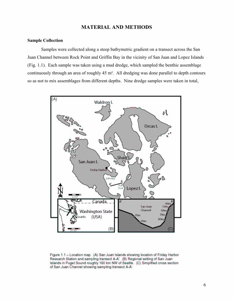
Samples were collected along a steep bathymetric gradient on a transect across the San
Juan Channel between Rock Point and Griffin Bay in the vicinity of San Juan and Lopez Islands
(Fig. 1.1). Each sample was taken using a mud dredge, which sampled the benthic assemblage
continuously through an area of roughly 45 m². All dredging was done parallel to depth contours
so as not to mix assemblages from different depths. Nine dredge samples were taken in total,

7
Depth Live Dead Total40m 10 11 21
50m 6 10 16
60m 1 6 7
Shallow (40-60m) 17 27 44
70m 28 40 68
80m 41 19 60
Deep (70-80m) 69 59 128
Total 86 86 172
Table 1.1 - Depth distribution of samples.
ranging from 20-120 m. From these samples, a total of five depth groups (40m, 50m, 60m, 70m,
and 80m) yielded abundant specimens of Terebratalia transversa. The majority of the
specimens were from the east side of the San Juan Channel (Fig. 1.1C), but some came from the
shallower sloped western side of the channel. However, sample sizes were not sufficient on the
western side to create ‘stand alone’ samples, so samples from 70m on the western side were
grouped with 70m samples from the eastern side and samples from 90m on the western side were
grouped with samples from 80m on the eastern side. This procedure is justified by the similarity
of sediment size fractions (mostly cobbles and boulders) in the dredge samples from which
material for this study was obtained. For further discussion of environments along the transect
see Kowalewski et al. (2003) and Rothfus et al. (in prep.).
Both live and dead specimens were collected from each dredge that yielded brachiopods.
For consistency, only whole, articulated shells of Terebratalia transversa were chosen for
morphometric analysis. For the purpose of simplifying analyses, an equal number of live and
dead shells were chosen. In all samples there were fewer dead, articulated shells than live shells.
Thus, the number of useable dead shells was the limiting factor when assembling specimens for
analysis. A total of 172 shells were analyzed (nLive=86; nDead =86). The distribution of the shells
by depth is given in Table 1.1.

8
Data Collection
Specimens were imaged in two orientations using a Polaroid DMC 1 digital camera. For
the anterior view, each specimen was placed with the anterior up and the camera was oriented
parallel to the commissural plane (Fig. 1.2A). For the dorsal view, each specimen was placed
with the dorsal (brachial) valve up and the camera was oriented perpendicular to the commissural
plane (Fig. 1.2B).
Morphometric analyses presented here are based on two sets (one for each view) of
landmarks and pseudolandmarks that were taken on each shell. Seven landmarks were used for
the anterior view and nine were used for the dorsal view (Fig. 1.2, Table 1.2). Both true
landmarks and pseudo-landmarks (Type I and II respectively) were used together in both views
to maximize the ability to quantify shape differences between individuals. The usefulness of
combining different types of landmarks in the same analysis varies with the question being asked
(Bookstein, 1990, 1991). In this study, a mix of homologous points and geometric points were
considered necessary to fully capture the morphological variation of the organism. This
methodology is justified by the operator error study (discussed below) which shows equal scatter
of replicates around Type I and Type II landmarks. Landmarks were taken using the image
analysis program SCION Image for Windows beta 4.0.2, developed by the U.S. National
Institutes of Health and Scion Corporation and available as freeware from
http://www.scioncorp.com.

9
External views were used exclusively because morphological differences among
individuals of Terebratalia transversa are most easily recognized in external properties of the
shell. Also, previous analyses of the morphology of T. transversa all used external features
exclusively, to define morpho-groups.
Landmark Type LocationAnterior view
1 II Leftmost adjoining point between dorsal and ventral valve2 II Point of maximum curvature of the commissure between landmarks 1 and 33 II Ventralmost point of maximum curvature of sulcus4 II Point of maximum curvature of the commissure between landmarks 3 and 55 II Rightmost adjoining point between dorsal and ventral valve6 II Point of maximum curvature of dorsal valve near the plane of symmetry7 II Point of maximum curvature of ventral valve near the plane of symmetry
Dorsal view
1 II Posteriormost point of ventral umbo2 I Left-lower margin of pedicle foramen3 I Right-lower margin of pedicle foramen4 II Posteriormost point of dorsal umbo5 I Left-lateral adjoining point of interarea and dorsal valve6 I Right-lateral adjoining point of interarea and dorsal valve7 II Leftmost point of maximum curvature8 II Rightmost point of maximum curvature9 II Anteriormost point of maximum curvature of dorsal valve
Table 1.2 - Landmark descriptions.
Analytical Methods
Procrustes Analysis: Shape was analyzed for both views using Procrustes analysis, a
superimposition technique that allows the comparison of landmark configurations by overlaying
one on top of the other. There are several different variants of Procrustes analysis, each useful
for a specific set of circumstances (Bookstein, 1990, 1991, 1996; Chapman, 1990; Rohlf, 1990b,
1996, 1999; Rohlf and Slice, 1990). For this study, a Generalized Least Squares Full Procrustes
Analysis (GLS-FPA) was utilized. This procedure calculates a reference (mean) configuration
from all of the samples. Each configuration of landmarks, corresponding to each sample, is then
rotated, translated and rescaled such that the distance from each sample to the reference
configuration is minimized using a least squares algorithm. In full Procrustes analysis, centroid
size is used to rescale each configuration to control for differences in size. Centroid size is
defined as the square root of the summed squared distances from each landmark to their common
10
centroid (Dryden and Mardia, 1998). It is a very convenient measure of overall size of an
organism because it is uncorrelated with shape variables and thus cannot indicate allometry when
none is present. Because of this, centroid size was also used later in the analysis to correct for
allometry in variability estimates. The SAS/IML code used for least squares Procrustes analysis
was modified from a code written by M. Kowalewski and A. Bush (Bush et al., 2002).
To graphically display the results from the Procrustes analysis, the partial tangent
coordinates were plotted on an x-y scatterplot. In most cases, especially where it was desirable
to show the relationship of several groups on one superimposition plot, the data points
themselves were omitted and replaced with polygons encircling their distribution. This was done
to improve the clarity and readability of these plots.
Comparison of fitting techniques: Least squares Procrustes analysis (GLS-FPA) is
regarded as the approach of choice when variance in shape is spread more or less equally among
landmarks (Chapman, 1990), that is, no particular landmark has more variance than the others.
In situations where change in shape is localized to one or a few landmarks, a different
Procrustean method must be used. In order to evaluate the appropriateness of two different
fitting techniques for the data presented here, a Resistant Fit-Full Procrustes Analysis (RF-FPA)
was also run on the landmark data for both shell views using Resistant-Fit Theta-Rho-Analysis,
available with the program CoordGen6, which is part of the Integrated Morphometrics Package
(IMP) developed by D. Sheets and available as freeware at
http://www.canisius.edu/~sheets/morphsoft.html.
The results of both analyses are very similar (Fig. 1.3) indicating a roughly equal spread
of variance across all landmarks in both shell views. Therefore, the Least Squares method was
used exclusively for the remainder of the study because outputs from GLS-FPA can be easier to
deal with in multivariate analysis than those from RF-FPA.
Operator Error Estimation: Repeatability is a potential problem in most morphometric
studies. Whether one’s primary unit of investigation is a specimen or a photograph, substantial
error can be introduced to the experiment if a standardized procedure is not used consistently.
To assess the amount of operator error involved with all of the stages of this analysis, one
shell from each of four randomly chosen sites was selected, re-imaged and re-measured ten
times. Each replication for each shell was done on different, non-consecutive days. Shells were
chosen so that two live and two dead samples would be replicated, and both views were
replicated for all four samples. The ten replicates for each shell view were pooled with the full

11
dataset and subjected to Procrustes analysis. The results from two of the replications are shown
in Figure 1.4. The tight grouping of replicate landmarks in each case indicates that measurement
error is slight in comparison to total morphological variability (for the variability values of the
replicates, see Table 1.3). Additionally, the equal scatter around Type I and Type II landmarks
provides justification for using both types together in this study.
Principal Components Analysis: Another way to examine the variability of landmark
points in tangent space is to run a principal components analysis (PCA) on the tangent
coordinates derived from Procrustes analysis. In fact, this method may be more reliable for
visualizing variation in landmarks than superimposition methods even though it does not allow
examination of variation at single landmark positions.
Tangent coordinates for each shell view (anterior and dorsal) were analyzed in the PROC
PRINCOMP procedure available in SAS 8.02 using the covariance matrix option. Scores for the
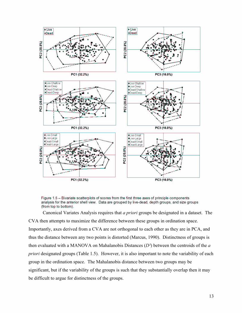
first three principle components were then plotted on bivariate scatterplots (Figs. 1.5-1.6).
Canonical Variates Analysis: For the purpose of comparing mean shapes, Canonical
Variates Analysis (CVA) was used. Again, the tangent coordinates for both views were the two
datasets used for this analysis. Prior to running CVA, the tangent coordinate matrix for each

12
view had to be pared down because the tangent coordinates (as well as the full Procrustes
residuals) are subject to four almost-linear constraints (Bookstein, 1996). Because of these
constraints, inversion of the covariance matrix yields meaningless coefficients (Bookstein, 1996;
Rohlf, 1999). One of the ways to avoid this pitfall, which is used here, was outlined by
Bookstein (1996) and by Rohlf (1999). Two vectors (four eigenvalues) from the tangent
coordinates must be removed. In principle, any four eigenvalues can be removed, however,
Rohlf (1999) recommended removal of the four smallest values as they account for very little of
the variation in the dataset. This recommendation was followed here. PCA was run on each of
the tangent coordinate datasets and the four smallest eigenvalues were removed in each case.
CVA was then run on the pared-down datasets.
NTotal
VariabilityAllometry Free
Variability
Dorsal ViewB102D 10 0.0127 0.0117C106D 10 0.0174 0.0141D107L 10 0.0212 0.0189E117L 10 0.0262 0.0253
B102D 10 0.0304 0.0253C106D 10 0.0278 0.0277D107L 10 0.0291 0.0266E117L 10 0.0312 0.0265
Anterior View
Table 1.3 - Variability values for the replicate samples.
13
Canonical Variates Analysis requires that a priori groups be designated in a dataset. The
CVA then attempts to maximize the difference between these groups in ordination space.
Importantly, axes derived from a CVA are not orthogonal to each other as they are in PCA, and
thus the distance between any two points is distorted (Marcus, 1990). Distinctness of groups is
then evaluated with a MANOVA on Mahalanobis Distances (D²) between the centroids of the a
priori designated groups (Table 1.5). However, it is also important to note the variability of each
group in the ordination space. The Mahalanobis distance between two groups may be
significant, but if the variability of the groups is such that they substantially overlap then it may
be difficult to argue for distinctness of the groups.

14
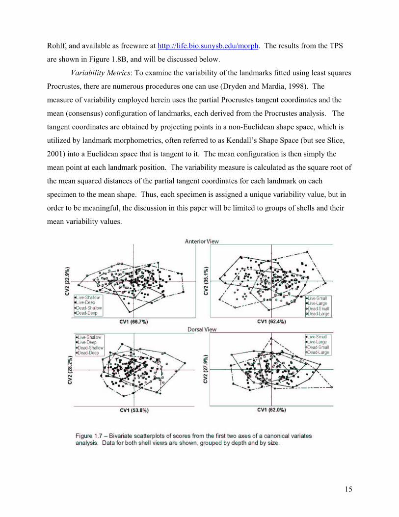
A total of four canonical variates analyses were run for this study. Each dataset (anterior
and dorsal) was run twice, first with depth groups designated and then with size groups
designated. These groupings will be explained later in the text. Scores for the first two
canonical axes (CV1 & CV2) were then plotted on bivariate scatterplots and groups were
indicated with polygons encircling the data points (Fig. 1.7).
Thin-Plate Spline Analysis: Another method of comparing mean shapes is the geometric
morphometric method of thin-plate spline analysis (TPS)(Bookstein 1990; 1991; 1996). TPS can
be very useful for visualizing the magnitude and direction of change between two shapes.
The two shapes used for this analysis were the mean landmark configurations from the Live and
Dead groups. The analysis was run using the program tpsSplin version 1.18 developed by F.J.
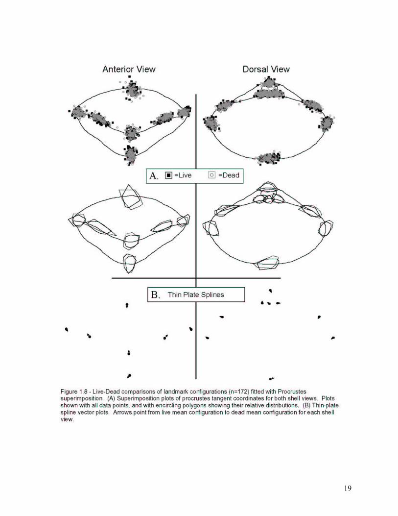
15
Rohlf, and available as freeware at http://life.bio.sunysb.edu/morph. The results from the TPS
are shown in Figure 1.8B, and will be discussed below.
Variability Metrics: To examine the variability of the landmarks fitted using least squares
Procrustes, there are numerous procedures one can use (Dryden and Mardia, 1998). The
measure of variability employed herein uses the partial Procrustes tangent coordinates and the
mean (consensus) configuration of landmarks, each derived from the Procrustes analysis. The
tangent coordinates are obtained by projecting points in a non-Euclidean shape space, which is
utilized by landmark morphometrics, often referred to as Kendall’s Shape Space (but see Slice,
2001) into a Euclidean space that is tangent to it. The mean configuration is then simply the
mean point at each landmark position. The variability measure is calculated as the square root of
the mean squared distances of the partial tangent coordinates for each landmark on each
specimen to the mean shape. Thus, each specimen is assigned a unique variability value, but in
order to be meaningful, the discussion in this paper will be limited to groups of shells and their
mean variability values.

16
Like many organisms, Terebratalia transversa, grows allometrically. The effects of this
shape change with growth will be discussed in further detail below, although an exhaustive
treatment is beyond the scope of this paper. Because of allometric growth, all of the size-related
variability is not removed by the normal Procrustes operation of setting each configuration to
unit centroid size. There is still some amount of shape variability due to size that is included in
the partial tangent coordinates. One way to remove the allometric component, and thus obtain an
allometry-free variability, is to regress the partial tangent coordinates on centroid size (Dryden
and Mardia, 1998). After the correction for allometry, the square root of the mean squared
distances was again calculated to yield allometry free variability (Table 1.3, 1.4).
Finally, all statistical analyses performed for this study utilize an arbitrarily selected
significance level (α) of 0.05.
17
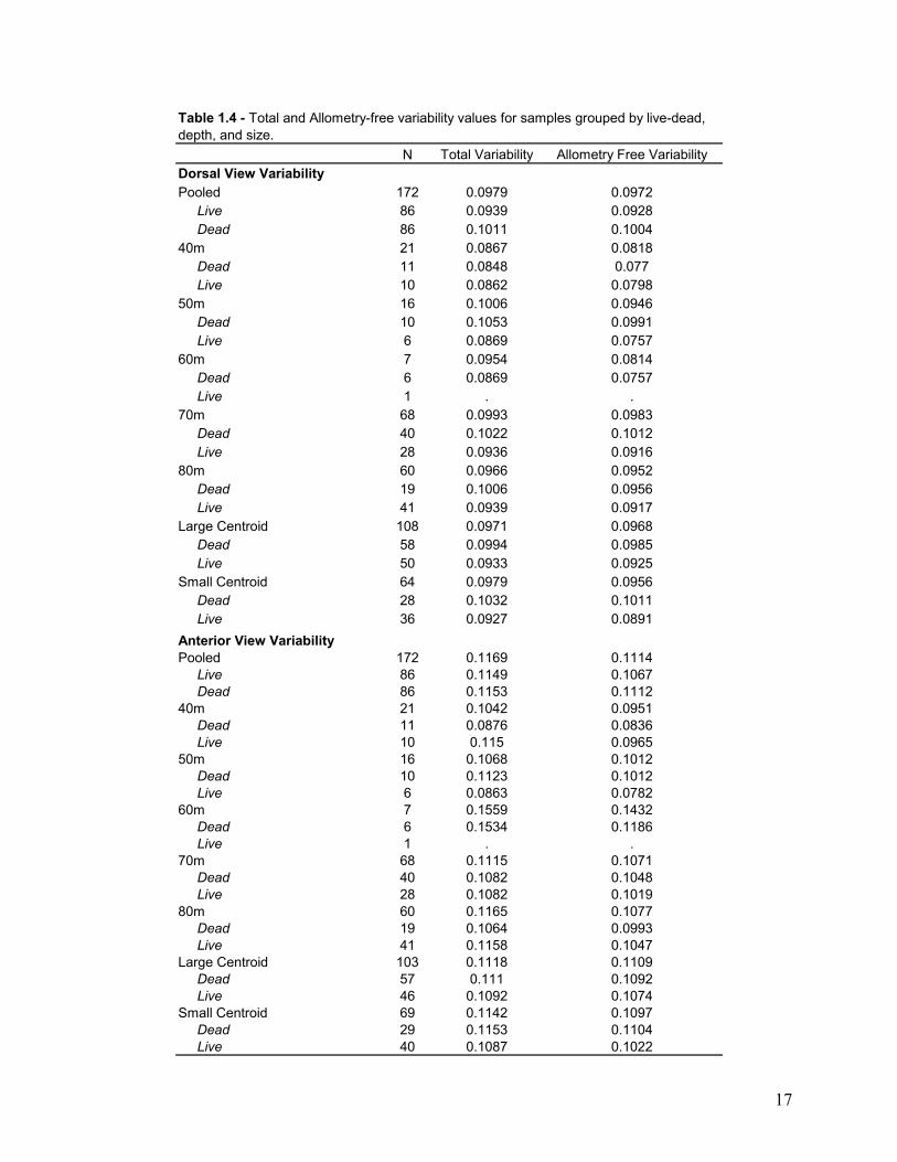
N Total Variability Allometry Free VariabilityDorsal View VariabilityPooled 172 0.0979 0.0972 Live 86 0.0939 0.0928 Dead 86 0.1011 0.100440m 21 0.0867 0.0818 Dead 11 0.0848 0.077 Live 10 0.0862 0.079850m 16 0.1006 0.0946 Dead 10 0.1053 0.0991 Live 6 0.0869 0.075760m 7 0.0954 0.0814 Dead 6 0.0869 0.0757 Live 1 . .70m 68 0.0993 0.0983 Dead 40 0.1022 0.1012 Live 28 0.0936 0.091680m 60 0.0966 0.0952 Dead 19 0.1006 0.0956 Live 41 0.0939 0.0917Large Centroid 108 0.0971 0.0968 Dead 58 0.0994 0.0985 Live 50 0.0933 0.0925Small Centroid 64 0.0979 0.0956 Dead 28 0.1032 0.1011 Live 36 0.0927 0.0891Anterior View VariabilityPooled 172 0.1169 0.1114 Live 86 0.1149 0.1067 Dead 86 0.1153 0.111240m 21 0.1042 0.0951 Dead 11 0.0876 0.0836 Live 10 0.115 0.096550m 16 0.1068 0.1012 Dead 10 0.1123 0.1012 Live 6 0.0863 0.078260m 7 0.1559 0.1432 Dead 6 0.1534 0.1186 Live 1 . .70m 68 0.1115 0.1071 Dead 40 0.1082 0.1048 Live 28 0.1082 0.101980m 60 0.1165 0.1077 Dead 19 0.1064 0.0993 Live 41 0.1158 0.1047Large Centroid 103 0.1118 0.1109 Dead 57 0.111 0.1092 Live 46 0.1092 0.1074Small Centroid 69 0.1142 0.1097 Dead 29 0.1153 0.1104 Live 40 0.1087 0.1022
Table 1.4 - Total and Allometry-free variability values for samples grouped by live-dead, depth, and size.
18
Mahalanobis Distance
(D ²) F P
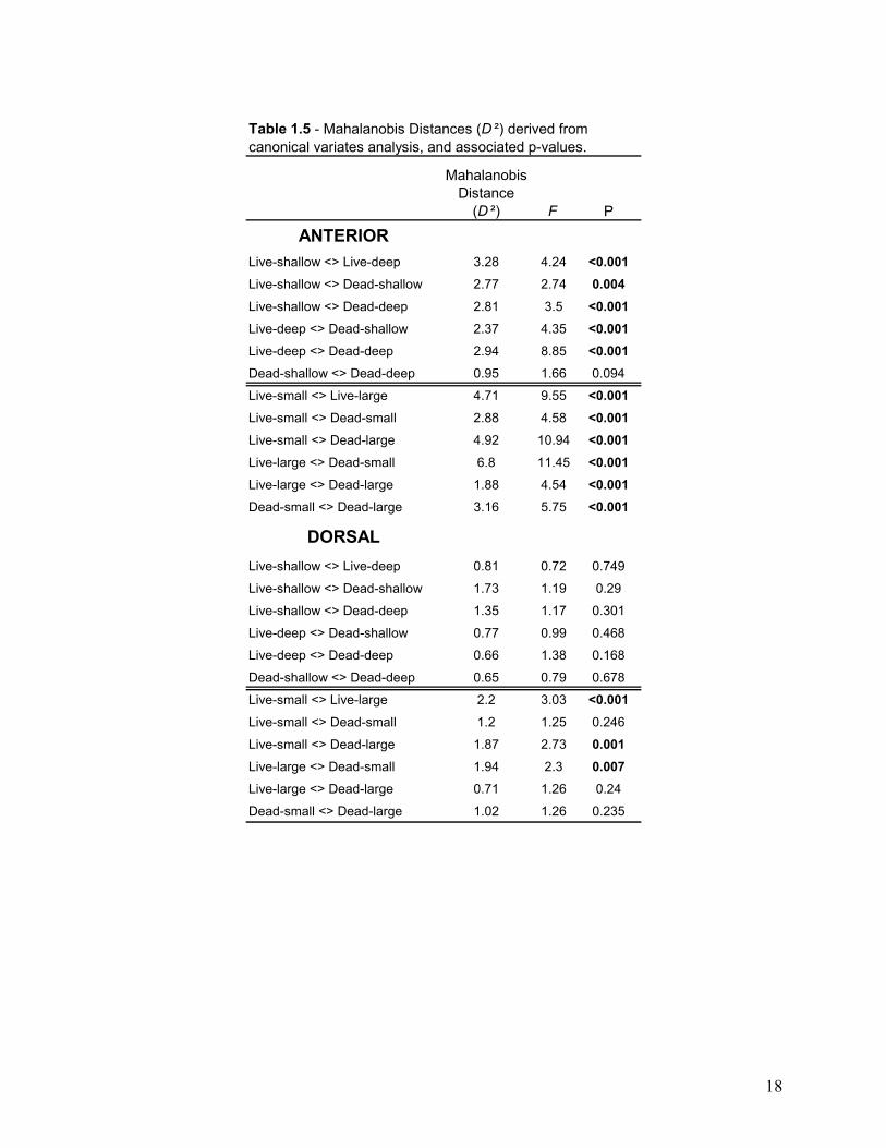
ANTERIORLive-shallow <> Live-deep 3.28 4.24 <0.001Live-shallow <> Dead-shallow 2.77 2.74 0.004Live-shallow <> Dead-deep 2.81 3.5 <0.001Live-deep <> Dead-shallow 2.37 4.35 <0.001Live-deep <> Dead-deep 2.94 8.85 <0.001Dead-shallow <> Dead-deep 0.95 1.66 0.094
Live-small <> Live-large 4.71 9.55 <0.001Live-small <> Dead-small 2.88 4.58 <0.001Live-small <> Dead-large 4.92 10.94 <0.001Live-large <> Dead-small 6.8 11.45 <0.001Live-large <> Dead-large 1.88 4.54 <0.001Dead-small <> Dead-large 3.16 5.75 <0.001
DORSALLive-shallow <> Live-deep 0.81 0.72 0.749
Live-shallow <> Dead-shallow 1.73 1.19 0.29
Live-shallow <> Dead-deep 1.35 1.17 0.301
Live-deep <> Dead-shallow 0.77 0.99 0.468
Live-deep <> Dead-deep 0.66 1.38 0.168
Dead-shallow <> Dead-deep 0.65 0.79 0.678
Live-small <> Live-large 2.2 3.03 <0.001Live-small <> Dead-small 1.2 1.25 0.246
Live-small <> Dead-large 1.87 2.73 0.001Live-large <> Dead-small 1.94 2.3 0.007Live-large <> Dead-large 0.71 1.26 0.24
Dead-small <> Dead-large 1.02 1.26 0.235
Table 1.5 - Mahalanobis Distances (D ²) derived from canonical variates analysis, and associated p-values.
19
20
RESULTS AND DISCUSSION
Mean Shape vs. Mean Variability
The results obtained for this study were arrived at through the use of a number of
techniques each of which was designed either to compare mean shapes between groups (GLS-
FPA, PCA, CVA, TPS) or to compare mean shape variability between groups (GLS-FPA, PCA,
Allometry-free variability). Some of the techniques can accomplish both with varying degrees of
success.
Through the course of this study it was determined that measures of morphological
variability would be more informative than changes in mean shape for detecting differences
between the time averaged assemblage and the standing crop population. Because the ‘dead’ or
time averaged assemblage is a combined sample of many generations, it is the variability of that
sample that must be examined to determine its degree of similarity, or fidelity, to the living
population. Nevertheless, it is useful to examine mean shapes of different populations of
Terebratalia transversa because much of the literature on this organism deals exclusively with
this metric, although it is generally assessed qualitatively.
Live-Dead Comparisons
Results: The main focus of this study is the assessment of morphological fidelity of a sub-
fossil assemblage of Terebratalia transversa. Consequently, those analyses that group the data
into Live and Dead categories are potentially the most informative.
Scores from principal components analysis for each shell view, grouped by membership
in Live and Dead categories, are shown in Figures 1.5 and 1.6. These plots show similar
amounts of variance between the two categories, regardless of which view is examined. One
possible exception is the plot of PC1 vs. PC2 for the anterior view (Fig. 1.5, top left panel).
Dead shells may be more variable than Live shells based on the larger plot area encompassed by
points of the Dead category. Additionally, the center of each cloud of points is in nearly the
same position, demonstrating that mean shapes may not be different between live and dead
shells. Furthermore, neither the live nor the dead groups have any discernible sub-groups
present, suggesting a lack of distinct morphogroups in either of the assemblages. However, far
reaching conclusions should not be drawn from such plots as PCA is not a confirmatory
multivariate analysis.

21
Thin-plate spline analysis was also used to compare mean shapes between live and dead
groups (Fig. 1.8B). In this analysis the mean configurations from Procrustes for each group was
compared. The vectors shown in Figure 1.8B indicate the magnitude and direction of shape
change at each landmark position from the live configuration to the dead configuration. As
indicated by PCA, the amount of mean shape change between these groups (in both views) is
minimal.
Potential shape variability changes between live and dead groups can be visualized by
plotting the tangent coordinates of a full, generalized Procrustes analysis (Fig. 1.8A). The
overlap between landmark configurations of both categories seems to be nearly complete,
suggesting little difference in shape variability between live and dead specimen groups
(allometry-free variability values are listed in Table 1.4). Additionally, the superimposition plots
do not show distinct morphogroups for either shell view. To evaluate the statistical significance
of the apparent similarity of variability for the two categories, 1000 mean allometry-free
variability values and 95% and 99% confidence intervals around the actual means were
calculated and compared for each group. This was accomplished with a 1000-iteration
bootstrapping simulation written in SAS/IML by M. Kowalewski and modified by the author.
The simulation was designed to randomly draw samples with replacement from a particular
group in the dataset until the actual number of samples for that group was reached (e.g. n=86 for
live and dead groups). The simulation then runs a GLS Procrustes analysis to compute a total
allometry-free variability value for each iteration. The 1000 simulated mean allometry-free
variability values for each group were then used to calculate confidence intervals around the
actual mean variability values. Figure 1.9A shows the results of the bootstrap simulations used
to compare the total dataset parsed into live and dead groups. For each shell view, the mean
variability values for live and dead shells show overlapping 95% and 99% confidence intervals
suggesting a high degree of similarity between the groups in terms of overall variability. In fact,
the actual mean variability values for either live or dead groups (in either view) fall at least at
their counterparts’s 95% confidence interval.
Discussion: It is clear that the live sample represents a single cohort of individuals and
thus, the variability that is shown in Figure 1.9A for the live sample can be taken as a reasonable
estimate of single-generation variability. That this live variability is much the same as the
variability of the death assemblage agrees well with the findings of other studies (Bell et al.,
1987; MacFadden, 1989; Bush et al., 2002). The slightly higher variance of dead shells can be

22
explained in one of two ways. It is possible that dead shells would be more prone to have
damage that would interfere with taking landmarks, such as chipping or abrasion. Such damage,
if present, could elevate the variability of the dead group. However, in the replicate experiments
discussed earlier, the dead shells (B102D, and C106D) had lower variances than the live shells
(Table 1.3, Figure 1.4). The elevated variability of dead shells could also represent the time-
averaging signature on these shells. If this is the case, then it may be that the effect of time-
averaging on morphological variability is less than may have been predicted by theoretical
models (see Kidwell, 1986; Bush et al., 2002).
Bush et al. (2002) also found similar morphological fidelity between the life and death
assemblages of the bivalves Mercenaria campechiensis and M. permagana, and presented a
series of theoretical models describing the expected effects of time-averaging on shape
variability in fossil assemblages (also refer to Kidwell, 1986). If the morphology of a given
taxon does not change for the duration of the time averaged interval, then the fidelity of the fossil
record with respect to morphology will be high. However, if shape changes during the interval
of time-averaging, a number of different effects can be produced. When one considers any given
morphological character that is normally distributed in the standing crop population but changes
in some way during a time averaged interval, there are several ways in which the time averaged

23
distribution of that character can be significantly different from any given single population. For
example, the central tendency of the distribution of this character can shift through time
effectively increasing the morphological variance of the time-averaged assemblage. Similarly,
gaps in the record can produce bimodal or multi-modal distributions of this character in the time-
averaged assemblage.
From the results presented in Figure 1.9A and in Bush et al. (2002), it is clear that shape
variability for Mercenaria and Terebratalia have changed very little for the duration of time-
averaging of their respective assemblages. Quantitative estimates of the durations of time-
averaging for molluscan assemblages have become increasingly available in the last decade
(Flessa et al., 1993; Flessa and Kowalewski, 1994; Meldahl et al., 1997; Kowalewski et al.,
1998). These studies dated molluscan shells (mostly Chione fluctifraga and C. californiensis)
from a variety of environments ranging from beach ridges to tidal flats and channels to fan deltas
in a faulted rift basin. The duration of time-averaging for these robust mollusks averaged at
~1000 years, but some environments, such as the tidal flat from Flessa et al. (1993), had averages
as high as ~3000 years.
Bush et al. (2002) were able to directly compare their assemblages to those of the time-
averaging studies listed above because Mercenaria and Chione are similar to each other in terms
of shell form, mineralogy, and durability. However, such a comparison may not be possible for
Terebratalia since the shell is smaller and thinner and has a different mineralogy (calcite rather
than aragonite) and microstructure than Mercenaria or Chione. Furthermore, even though the
calcite shell of Terebratalia makes it less susceptible to dissolution in modern oceans than
Mercenaria or Chione, the higher organic content of the shell greatly reduces its durability
shortly after the death of the organism (Daley, 1993).
Until recently, little was known about durations of time-averaging for brachiopods,
probably because they do not contribute a significant amount of skeletal material to the sediment
in most modern environments. An exception is the outer shelf and coastal bays of the Southeast
Brazilian Bight, where recent work has documented a low-diversity, high abundance assemblage
of terebratulide brachiopods that dominate that local fauna (Kowalewski et al., 2002). In a first
attempt to obtain time-averaging estimates for brachiopods, Carroll and colleagues (Carroll et al.,
2003; also see Barbour Wood et al., 2003), obtained dates for 82 individual shells of the most
common species of the Brazilian Bight, Bouchardia rosea. Using amino acid racemization
calibrated with AMS-radiocarbon, they found durations of time-averaging in brachiopods to be

24
strikingly similar (mean=460 years; standard deviation=680 years; maximum=3134 years) to
those documented for mollusks (Flessa et al., 1993; Flessa and Kowalewski, 1994; Meldahl et
al., 1997; Kowalewski et al., 1998). While the durations obtained for Bouchardia were highly
variable from site to site, the results of Carroll et al. (2003) suggest that shell mineralogy and
microstructure are probably not the primary factors controlling the nature and scale of time-
averaging. It may therefore be reasonable to extrapolate between studies and environments to
put at least a maximum estimate (≤3000 years) on the amount of time-averaging that the death
assemblage of T. transversa may have experienced. The variability estimates presented here
(Figs. 1.8-1.9, Table 1.4) indicate the morphological fidelity of the sub-fossil record of T.
transversa may be rather good on centennial to millennial time scales.
Depth Comparisons
Results: It is possible that morphology or morphological variability could change
between sub-groups of the dataset. The potential effect of depth on morphology may be
significant, especially in light of predictions discussed earlier (Du Bois, 1916; Schumann, 1990).
Figures 1.10 and 1.11 show superimposition plots of Procrustes tangent coordinates with
the dataset grouped into five depth categories corresponding to the depths sampled for this study.
It should be noted that sample sizes for the 40-60m sites are rather small (Table 1.1), and it is
therefore not desirable to use these categories for further analysis. However, these
superimposition plots (Figs. 1.10-1.11) suggest that neither mean shape nor mean variability are
substantially different among the shells from 40-60m and those from 70-80m. Therefore,
grouping the dataset such that samples are parsed into ‘shallow’ (40-60m) and ‘deep’ (70-80m)
groups seems most effective. All subsequent analyses for this section will be done using these
groups.
The mean shapes for the shallow and deep groups were investigated in much the same
manner as for the pooled, live-dead comparisons. Figures 1.5 and 1.6 show the results of PCA
grouped by depth and by live-dead. The PCA plots seem to suggest a difference in mean shape
between the depth groups, as defined by a difference in position of the center of one cloud of
points to another. In order to rigorously test for differences between group means, CVA was run
with depth groups chosen a priori. Figure 1.7 shows the scatter plots of CVA scores on CV1 and
CV2. Separation between depth groups is somewhat better here, and indeed, the Mahalanobis
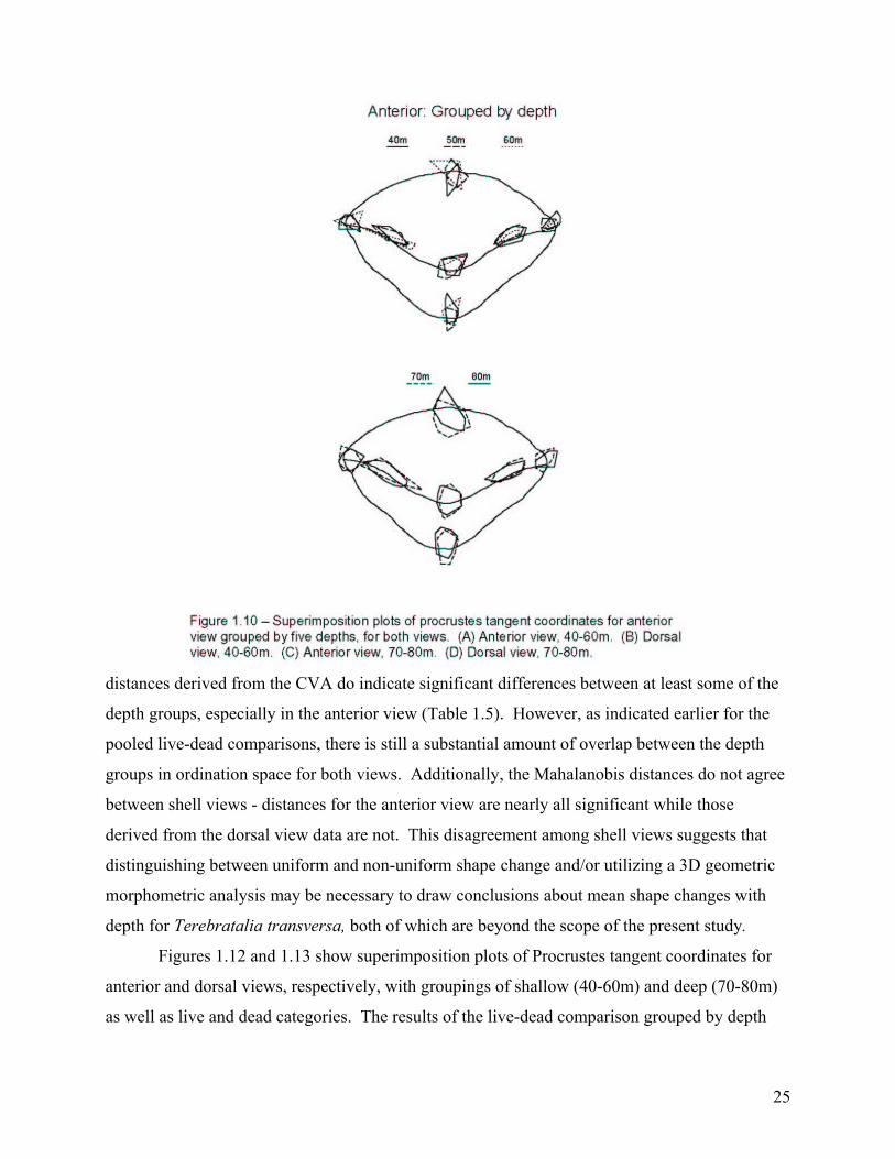
25
distances derived from the CVA do indicate significant differences between at least some of the
depth groups, especially in the anterior view (Table 1.5). However, as indicated earlier for the
pooled live-dead comparisons, there is still a substantial amount of overlap between the depth
groups in ordination space for both views. Additionally, the Mahalanobis distances do not agree
between shell views - distances for the anterior view are nearly all significant while those
derived from the dorsal view data are not. This disagreement among shell views suggests that
distinguishing between uniform and non-uniform shape change and/or utilizing a 3D geometric
morphometric analysis may be necessary to draw conclusions about mean shape changes with
depth for Terebratalia transversa, both of which are beyond the scope of the present study.
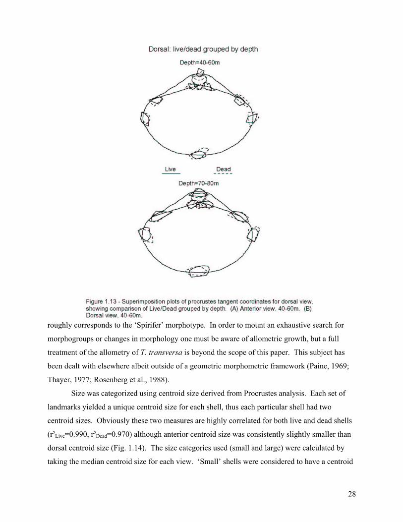
Figures 1.12 and 1.13 show superimposition plots of Procrustes tangent coordinates for
anterior and dorsal views, respectively, with groupings of shallow (40-60m) and deep (70-80m)
as well as live and dead categories. The results of the live-dead comparison grouped by depth

26
roughly mirror those of the pooled data (Fig. 1.8, 1.9B, C). No distinct morphogroups, live or
dead, can be recognized at different depths for either shell view. As in other analyses, dead
shells seem to be somewhat more variable than live, but this difference is negligible as mean
allometry-free variability values have substantially overlapping bootstrapped confidence
intervals for both shallow and deep groups and both views (Fig. 1.9B, C). It is interesting to note
that Figure 1.9B shows rather large confidence intervals for the shallow group of the dataset, and
it is tempting to interpret this result as a change in shape variability with depth. However, even
after grouping depths together to run these analyses, the shallow sample is still substantially
smaller than that for the deep group (Table 1.1). Thus, while these data may indicate a decrease
in shape variability with increasing depth for Terebratalia transversa, the difference in sample
size for the two depth groups does not allow rejection of the null hypothesis of similarity.

27
Discussion: Regardless of whether overall shape variability changes with depth, it is clear
that live and dead specimens from any given depth category have a very similar magnitude of
variability. Therefore, one can deduce that the fidelity of morphological disparity within
Terebratalia transversa is very good at any depth, as long as large-scale spatial mixing of
assemblages can be ruled out. While no evidence for such mixing was encountered during this
study (also see Kowalewski et al., 2003), it was not explicitly addressed.
Size Comparisons
Results: As mentioned earlier, Terebratalia transversa exhibits a slight allometry with
growth. Schumann (1990) noted this when he was delineating his morphotypes. Juvenile T.
transversa are, in general, more alate and less inflated, with less prominent sulci, a form which
28
roughly corresponds to the ‘Spirifer’ morphotype. In order to mount an exhaustive search for
morphogroups or changes in morphology one must be aware of allometric growth, but a full
treatment of the allometry of T. transversa is beyond the scope of this paper. This subject has
been dealt with elsewhere albeit outside of a geometric morphometric framework (Paine, 1969;
Thayer, 1977; Rosenberg et al., 1988).
Size was categorized using centroid size derived from Procrustes analysis. Each set of
landmarks yielded a unique centroid size for each shell, thus each particular shell had two
centroid sizes. Obviously these two measures are highly correlated for both live and dead shells
(r²Live=0.990, r²Dead=0.970) although anterior centroid size was consistently slightly smaller than
dorsal centroid size (Fig. 1.14). The size categories used (small and large) were calculated by
taking the median centroid size for each view. ‘Small’ shells were considered to have a centroid

29
size smaller than the median, while ‘large’ shells had a centroid size larger than the median (the
shell of median size was arbitrarily placed in the ‘large’ group for each view). Because each
shell had two size measures, and because they were not identical for any given shell, some shells
were assigned to the ‘large’ category for the anterior centroid size, but to the ‘small’ category for
dorsal centroid size, and vice versa. This is why sample sizes are different between the two large
and the two small groups (Table 1.4). In order to be able to draw meaningful size comparisons
between the live and dead shells used in the study, the size-frequency distributions (Fig. 1.14) of
each of the centroid sizes had to be investigated. Each of these distributions shows a left-skewed
distribution, a rather unusual distribution for biological populations which are generally right-
skewed. This is a result of a sampling bias, present because very small shells would not yield
useable images that were conducive to taking landmarks. Importantly, the shapes of the live and
dead size-frequency distributions for both views are not significantly different (Kolmogrov-
Smirnov Test: pDorsal=0.07; pAnterior=0.07), nor are their central tendencies (Kruskal-Wallis Test:
chi²Dorsal =1.53, p=0.22; chi²Anterior=1.79, p=0.18) making comparisons between them reasonable
(Fig. 1.14).
An analysis of mean shapes for size groups was also conducted, but the results are again
ambiguous as they were for depth groups. Figures 1.5, 1.6, and 1.7 show the results of PCA and
CVA respectively for the dataset grouped into small and large categories. Again, a test of

30
significance for the Mahalanobis distances derived from CVA does not yield clear results (Table
1.5). Both CVA and PCA show substantial overlap between groups in ordination space and this
variability may override the significant differences in mean shape between the groups.
Figure 1.15 shows the results of Procrustes analysis of landmarks from both views,
grouped by centroid size. The allometry mentioned earlier, and noted by Schumann (1990) is
easily seen. Small shells are wider, shorter, and less inflated than large shells which are
generally more globose. Figures 1.16 and 1.17 show the results from Procrustes analysis with
live-dead and size groups separated out. As was noted previously for other groupings of the
data, live and dead groups overlap substantially on these superimposition plots, and there is no
indication of distinct morphogroups for either view. Furthermore, mean allometry-free
variability values (Fig. 1.9D, E) are, again, very similar with a large degree of overlap in
confidence intervals for each pairwise (live-dead) comparison.
Discussion: Schumann (1990) postulated that all juvenile shells of Terebratalia
transversa have a shape similar to the ‘Spirifer’ morphotype, and that, as each individual grows,
its morphology usually diverges from that form in one of several different ways, in response to
environmental factors. While this study did not include juvenile shells, the results presented in
the previous section seem to be inconsistent with that hypothesis. The shape variability of T.
transversa is a trait that is present with the same magnitude in both small and large shells (Fig.
1.9D, E), and thus it is not likely to be a trait that changes during ontogeny. The implication is
that assemblages of small individuals should be just as morphologically variable as assemblages
of large individuals.

31

32
CONCLUSIONS
The shape variability of the terebratulide brachiopod Terebratalia transversa is
remarkably consistent in life and death assemblages. This trend persists when all data are
pooled, when individuals are grouped by depth, and when individuals are grouped by size.
Change in average shape between groups is more ambiguous, and often cannot be separated from
the shape variability of the groups in question. Additionally, this study found no evidence of
distinct morphogroups in populations of T. transversa. Rather, variability seems to be
continuous from one form to another. Furthermore, the range of variability is remarkably similar
at all sites sampled, which encompass the entire depth range of the species in the area, and for
different size groups.
Given the similar range of morphological variability at each site, it is possible that the
wide array of micro-environments available at any given place in the San Juan Channel (exposed
or cryptic, high or low current depending on orientation of cobble substrate), could exert a strong
control on the morphology of Terebratalia transversa. This control could work in concert with
the species’ apparent inability to reorient itself under changing conditions (Thayer, 1975, 1977;
LaBarbera, 1977) to produce the high degree of variability observed at each site. This is similar
to Schumann’s (1990) suggestion discussed earlier, but since a wide range of micro-
environments is probably available at any given site, populations from each site exhibit a similar
amount of morphological variance.
The consistency in morphological variability between the living population and its sub-
fossil record is documented here for the first time in brachiopods, and has important implications
for the fossil record of the group. It appears that morphological variance of the standing crop
population can be estimated from that population’s death assemblage, even in organisms whose
shells break down quickly after death (Daley, 1993). This also means that the brachiopod fossil
record may be relatively complete with respect to morphological variants of all of the constituent
species. The recognition of morphologically variable species, as such, may in that case be
possible in the fossil record, especially by utilizing the powerful geometric morphometric
techniques employed herein.

33
CHAPTER TWO1: Body size estimates from the literature: Utility and potential for macroevolutionary studies
1 This paper was submitted for publication to Palaios on 7 November 2005. The co-authors for this publication, Jennifer A. Stempien, Michał Kowalewski, and Arnold I. Miller, contributed less than 20% to the data collection and analysis stages of this project. The text was written completely by R.A. Krause.
34
ABSTRACT
Images in the monographic literature represent an important but relatively untapped,
resource for paleontologists. In particular, they could provide vast amounts of body size data.
However, it is possible that images of specimens represent a biased sample of the fossil record.
Thus, before body size estimates from the literature can be used in analyses, the quality of these
data must be assessed.
Two complementary datasets were constructed for a group of bivalve and brachiopod
species from the Paleozoic and the Cenozoic. The monograph dataset consisted of length
measurements taken from all unique images of a species in a monograph. The counterpart bulk
dataset consisted of comparable measurements taken from a set (n>10) of bulk-collected
specimens of the same species, acquired from the same locality, as those figured in the
monograph. These paired datasets for each species were used to assess the quality of
monographic data.
Bias direction and magnitude were assessed by using the bulk sample of a species as an
estimate of its underlying size-frequency distribution. Bias was estimated for each monographed
specimen by calculating its percentile-value in relation to the size-frequency distribution for that
species. All species groups had mean values within the 70th to 85th percentile range, indicating a
significant bias toward monograph specimens that are larger than the mean of the bulk sample.
The consistency of bias was evaluated by comparing the monograph sample mean to the bulk
sample mean for each species. When compared in bivariate scatter plots, all species groups
yielded significant regression lines with slopes near unity, indicating highly consistent, yet
predictable, bias in each case. This trend persisted when the data were grouped taxonomically,
geographically, or by year of monograph publication.
These results indicate that size measurements of monographed specimens of bivalves and
brachiopods consistently record similar size-classes for most species. This bias is easy to
remove, and doing so renders size data from images in monographs useful for macroevolutionary
studies of body size.

35
INTRODUCTION
Images of specimens are essential to the taxonomic literature. They enable an author to
concisely present descriptive and comparative information on specimens, which cannot be easily
expressed in words (Mayr et al., 1953). Images also remove an element of subjectivity from the
description of species – allowing the reader to see the specimen that is being described. For this
reason, it is not uncommon for taxonomic journals to require high-quality images to accompany
any description of a new species, and images are highly encouraged in papers not focusing on
alpha-taxonomy as well (Journal of Paleontology, Instructions for Authors,
http://www.journalofpaleontology.org/instruct.htm). In fact, many taxonomic publications
include numerous images in order to fully document the natural variability of a population. As a
result, published images afford a researcher the opportunity to view a representative suite of
specimens from any species, in collections from all over the world.
Despite their central importance in alpha taxonomy, published images of specimens have
been underutilized by paleontologists engaged in the analysis and synthesis of existing
taxonomic information. In the last few decades, these workers have established themselves as a
fundamental enterprise of modern paleontology (Adrain, 2001), by drawing heavily on the
taxonomic literature to examine large-scale patterns in the history of life. Yet the types of data
extracted from the literature have remained rather limited. Most often, biodiversity studies
(Newell, 1959; Valentine, 1969; Sepkoski, 1982; Sepkoski, 1992; Benton, 1993; Sepkoski, 2002)
have utilized taxon names and ranges compiled from numerous publications. Other studies have
used taxon occurrences in fossil collections (Alroy et al., 2001), species richness at single
localities (Bambach, 1977), and relative abundance in bulk-collected samples (Powell and
Kowalewski, 2002). The full scope of data types in the taxonomic literature are just beginning to
be explored in large, community-wide initiatives such as the Paleobiology Database
(http://paleodb.org). Yet, the images in taxonomic publications remain as untapped resources
with great potential.
Such images could be used as a primary or supplementary data source in many types of
studies that have traditionally been considered “specimen-based”. For example, because
taxonomists take great care to visually document all diagnostic features of a species, published
images can yield a wealth of morphological information, from simple linear dimensions to
landmark coordinates for geometric morphometric analysis.

36
The inclusion of image-derived data in a study is advantageous to the researcher in
several ways. Images in monographs allow quick examination of large numbers of specimens
that have been taxonomically identified by an expert on that group. These specimens may be
reposited in museum collections that are geographically remote or otherwise difficult to access,
but their images can be studied in any major university library. In addition, these images are
often tied directly to detailed information on locality and sampling horizon (Kowalewski, 2002)
that closely approximates the level of detail commonly available in a museum or field collection.
Despite their promise, data derived from images may be biased in several ways,
depending on the type of information being extracted. The purpose of the present paper is to
investigate the biases inherent in the collection of simple linear measurements from published
images. Specifically, the quality of these data will be assessed with respect to three parameters:
(1) bias direction – the presence of non-random departures from the actual mean size of a
species; (2) bias magnitude – the absolute value of the mean departure, that is, the imprecision of
the data; and (3) bias consistency – the variation in the direction and magnitude of bias within
and across monographs, higher taxa, or time intervals. Only with a clear understanding of these
bias parameters will it be possible to assess the utility of monograph-derived size data.

37
TYPES OF PHOTOGRAPHIC BIAS
Apparent Versus Actual Size
One potential problem with photographs is that they may not accurately reproduce the
sizes of the specimens. Distortions can occur at many stages of the photographic process,
including improper orientation of a specimen or camera, poor lighting, or a failure to accurately
report magnification.
While it is difficult to address each of these problems in isolation, several studies have
addressed this issue by studying the concordance of measurements of specimens and their
images. Kowalewski and colleagues (2000) studied predatory drill hole size in Permian
brachiopods and showed that photographic distortion introduces negligible error even when
measuring items less than a millimeter in diameter. Similar studies have been conducted on
grain size distributions in coarse sediment samples (Ibbeken and Schleyer, 1986; McEwan et al.,
2000; Butler et al., 2001; Sime and Ferguson, 2003). These studies found a significant
difference between grain size distributions taken from photographs and those taken from direct
grain measurement of the same sample. Fortunately, image-derived grain size distributions
always deviate from traditionally collected grain size distributions in a predictable way –
distributions derived from images are always too fine by some amount, (this is because shadows
cast on grain boundaries make all grains appear smaller in images than they actually are). The
magnitude of this bias is invariant across a range of environments and thus, can be easily
corrected (Sime and Ferguson, 2003).
Sampling Bias
In addition to the disparity between the apparent versus actual size of an object, there is
another issue to consider: the potential for bias introduced by the choice of specimens
photographed by the author of a monograph.
The author’s choice of specimens to photograph may be a biased sample with respect to
size. This can be purely accidental, perhaps caused by an unconscious tendency to pick certain
size classes over others, or a deliberate attempt to illustrate certain size classes that display
specific morphological features. In this study the latter possibility has been controlled for, by
excluding monographs that intend to study size relationships in a population, such as ontogenetic
series. Thus, it is the potential worker-induced bias that is under scrutiny here. Such a bias, if

38
present, can lead to serious problems for the researcher interested in extracting meaningful size
data from the monographic literature.
TABLE 2.1 - Attributes of the bulk sample and monograph sample for each species. Bulk sample: nbulk is the number of specimens measured by us, or the
author of the monograph; ntotal is the total number of specimens that were available from a particular sample, when unreported, this category is scored as "-". Monograph sample: nmon is the number of measured monograph specimens for each species. Abbreviations: O - Ordovician; S - Silurian; D - Devonian; M- Mississippian; P - Paleocene; E - Eocene; Mio. - Miocene; Plio. - Pliocene; R - Recent. References: 1=Alberstadt, 1979; 2=Amano, 1986; 3=Amsden, 1968;
4=Babin & Melou, 1972; 5=Balinski, 1995; 6=Balinski, 1997; 7=Bird, 1965; 8=Cooper, 1988; 9=Craig, 2000; 10=Gordon et al., 1993; 11=Howe, 1979; 12=Johnston, 1993; 13=Jung, 1996; 14=Lauriat-Rage, 1982; 15=Li & Jones, 2003; 16=Liljedahl, 1983; 17=Liljedahl, 1984; 18=Pope, 1982; 19=Sanchez, 1986;
20=Sanchez, 1990; 21=Sanchez et al., 1995; 22=Soot-Ryen, 1964.
nmon nbulk ntotal period ref. region nmon nbulk ntotal period ref. regionAdairia adairensis 2 24 117 M 10 Ozark region, USA Anadara transversa 2 54 _ Mio. 7 Natural Well, NC, USA
Antirhynchonella thomasi 9 29 200 S 3 Ozark region, USA Anadara transversa 1 20 _ Plio. 7 Town Creek, NC, USA
Atrypina erugata 5 19 50 S 3 Ozark region, USA Anadara transversa 1 20 _ Plio. 7 James City, NC, USA
Basiliola sp. 3 15 _ P 9 Carnarvon Basin, w. Australia Astarte fusca incrassata 6 50 _ Plio. 14 St. Michel, Pays de la Loire, France
Biernatella lentiformis 7 103 _ D 5 Holy Cross Mtns., Poland Astarte omalii omalii 21 29 _ Plio. 14 Nantes, Pays de la Loire, France
Biernatella ovalis 4 15 _ D 5 Holy Cross Mtns., Poland Astarte omalii scalaris 25 176 _ Plio. 14 Nantes, Pays de la Loire, France
Biernatella polonica 1 26 _ D 5 Holy Cross Mtns., Poland Astarte omalii scalaris 33 128 _ Plio. 14 Angers, Pays de la Loire, France
Dicamaropsis parva 13 93 200 S 3 AR and OK, USA Astarte solidula 5 100 _ Plio. 14 Nantes, Pays de la Loire, France
Dicoelosia bilobella 5 33 100 S 3 AR and OK, USA Astarte sulcata redonensis 4 50 _ Plio. 14 St. Michel, Pays de la Loire, France
Dicoelosia oklahomensis 3 13 _ S 3 AR and OK, USA Astarte sulcata redonensis 1 51 _ Plio. 14 le Houx, Pays de la Loire, France
Eospirifer acutolineatus acutolineatus 5 29 100 S 3 AR and OK, USA Cadomia typa 2 16 16 O 19 western Argentina
Eospirifer acutolineatus pentagonus 6 30 300 S 3 AR and OK, USA Cardiomya (C.) islahispaniolae 6 25 _ Mio. 13 Dominican Republic
Giraliathgyris kaitrinae 2 54 _ P 9 Carnarvon Basin, w. Australia Cardiomya (Bowdenia) distira 4 28 _ Mio.-Plio
13 Dominican Republic
Giraliathryris jubileensis 3 44 _ E 9 Carnarvon Basin, w. Australia Cornellites catellus 1 14 34 D 12 southeastern Australia
Giraliathyris mcnamarai 1 81 _ P 9 Carnarvon Basin, w. Australia Crassatellopsis lenticularis 8 15 15 D 12 southeastern Australia
Hircinisca havliceki 4 22 45 S 3 AR and OK, USA Cypricardinia minima 3 18 18 D 12 southeastern Australia
Inflatia cherokeensis 2 48 100 M 10 Ozark region, USA Digitaria digitaria 2 68 _ Plio. 14 le Pigeon-Blanc, Pays de la Loire, FranceInflatia clydensis 2 12 102 M 10 Ozark region, USA Digitaria digitaria 1 38 _ Plio. 14 la Gauviniere, Pays de la Loire, FranceInflatia cooperi 2 15 42 M 10 Ozark region, USA Eoschizodus taemasensis 2 14 18 D 12 southeastern Australia
Inflatia gracilis 1 12 32 M 10 Ozark region, USA Freja fecunda 3 65 164 S 17 Gotland, Sweden
Inflatia inflata 2 27 40 M 10 Ozark region, USA Glycymeris americana 3 40 _ Plio 7 Old Dock, NC, USA
Inflatia pusilla 1 24 165 M 10 Ozark region, USA Glycymeris anteparilis 2 21 _ Mio 7 Silverdale, NC, USA
Kozlowskiellina (K.) vaningeni 6 47 200 S 3 AR and OK, USA Glycymeris idensis 3 50 _ Mio. 2 Hokkaido, Japan
Meristina clairensis 3 21 60 S 3 AR and OK, USA Glycymeris pectinata 2 20 _ Plio 7 Acme, NC, USA
Nanospira clairensis 11 67 200 S 3 AR and OK, USA Glycymeris subovata 2 21 _ Mio 7 James River, VA, USA
Nucleospira lens 1 36 645 D 15 Arctic Canada Goniophora duplisulca 3 27 29 D 12 southeastern Australia
Oepikina minnesotensis 26 80 _ O 18 northern KY, USA Gotodonta gotlandica 4 62 214 S 22 Gotland, Sweden
Oepikina minnesotensis 13 94 _ O 18 northern KY, USA Haliris jamaicensis 3 10 _ Plio. 13 Dominican Republic
Orthorhynchula linneyi 3 38 _ O 11 northern KY, USA Janeia silurica 3 18 597 S 17 Gotland, Sweden
Orthorhynchula sublinneyi 7 39 _ O 11 northern KY, USA Modiolopsis cuyana 1 17 17 O 20 western Argentina
Pionomena recens 10 65 _ O 18 northern KY, USA Myoplusia contrastans 4 17 35 O 4 Crozon, France
Platystrophia annieana 4 33 _ O 1 northern KY, USA Mytilarca bloomfieldensis 6 13 18 D 12 southeastern Australia
Platystrophia colbienesis 4 14 _ O 1 northern KY, USA Noetia (Eontia) carolinensis 1 20 _ Mio 7 Black Rock, NC, USA
Platystrophia elegantula 1 10 _ O 1 northern KY, USA Noetia (Eontia) limula 1 20 _ Plio 7 James City, NC, USA
Platystrophia ponderosa 7 34 _ O 1 northern KY, USA Noetia (Eontia) platyura 1 20 _ Plio 7 Town Creek, NC, USA
Plicatoria wilmingtonensis 25 80 251 E 8 Wilmington, NC, USA Noetia (Eontia) trigintinaria 2 16 _ Mio 7 Natural Well, NC, USA
Plicatoria wilmingtonensis 8 235 235 E 8 Wilmington, NC, USA Nuculites argentinum 7 19 25 S 21 western Argentina
Rhyncotrema increbescens 7 29 _ O 11 northern KY, USA Nuculodonta gotlandica 6 197 218 S 16 Gotland, Sweden
Sowerbyella sp. 5 23 _ O 11 northern KY, USA Nuculoida lens 6 142 153 S 16 Gotland, Sweden
Terebratulina lachryma 1 24 24 E 8 SC, USA Plectodon granulatus 4 20 _ R 13 Carribean Sea
Terebratulina wilsoni 2 48 48 E 8 SC, USA Similodonta djupvikensis 1 15 26 S 22 Gotland, Sweden
Victorithyris blakeorum 4 39 _ P 9 Carnarvon Basin, w. Australia Trigonulina bowdenensis 8 54 _ Mio.-Plio
13 Dominican Republic
Victorithyris decapello 2 54 _ P 9 Carnarvon Basin, w. Australia Trigonulina ornata 4 74 _ R 13 Carribean Sea
Waiotrypa sulcicarina 3 31 _ D 6 Holy Cross Mtns., Poland Trigonulina pacifica 5 155 _ R 13 Santa Catalina Island, CA, USA
Brachiopodsspecies
Bivalvesspecies
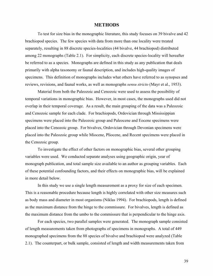
39
METHODS
To test for size bias in the monographic literature, this study focuses on 39 bivalve and 42
brachiopod species. The few species with data from more than one locality were treated
separately, resulting in 88 discrete species-localities (44 bivalve, 44 brachiopod) distributed
among 22 monographs (Table 2.1). For simplicity, each discrete species-locality will hereafter
be referred to as a species. Monographs are defined in this study as any publication that deals
primarily with alpha taxonomy or faunal description, and includes high-quality images of
specimens. This definition of monographs includes what others have referred to as synopses and
reviews, revisions, and faunal works, as well as monographs sensu stricto (Mayr et al., 1953).
Material from both the Paleozoic and Cenozoic were used to assess the possibility of
temporal variations in monographic bias. However, in most cases, the monographs used did not
overlap in their temporal coverage. As a result, the main grouping of the data was a Paleozoic
and Cenozoic sample for each clade. For brachiopods, Ordovician through Mississippian
specimens were placed into the Paleozoic group and Paleocene and Eocene specimens were
placed into the Cenozoic group. For bivalves, Ordovician through Devonian specimens were
placed into the Paleozoic group while Miocene, Pliocene, and Recent specimens were placed in
the Cenozoic group.
To investigate the effect of other factors on monographic bias, several other grouping
variables were used. We conducted separate analyses using geographic origin, year of
monograph publication, and total sample size available to an author as grouping variables. Each
of these potential confounding factors, and their effects on monographic bias, will be explained
in more detail below.
In this study we use a single length measurement as a proxy for size of each specimen.
This is a reasonable procedure because length is highly correlated with other size measures such
as body mass and diameter in most organisms (Niklas 1994). For brachiopods, length is defined
as the maximum distance from the hinge to the commissure. For bivalves, length is defined as
the maximum distance from the umbo to the commissure that is perpendicular to the hinge axis.
For each species, two parallel samples were generated. The monograph sample consisted
of length measurements taken from photographs of specimens in monographs. A total of 449
monographed specimens from the 88 species of bivalve and brachiopod were analyzed (Table
2.1). The counterpart, or bulk sample, consisted of length and width measurements taken from

40
88 bulk-collected samples, one for each of the species. Each bulk sample consisted of at least 10
specimens and was always from the same locality or region as the specimens for that species
measured in the monograph. All of the bulk samples used in this study came from tables or plots
of raw measurements reported in the publications used to construct the monograph sample.
Thus, the monograph and bulk samples are directly comparable because they were drawn from
the same underlying population of a species at a locality.
All statistical analyses were performed with codes written by MK and RAK in SAS and
SAS/IML version 9.1. A significance criterion of 5% (α = 0.05) was used for the determination
of statistical significance.
Specimen-Level Analysis
Size frequency distributions were constructed for each species from their bulk samples
(Fig. 2.1A). The percentile value of each monograph measurement for a species was then
defined by comparing it directly to the size-frequency distribution of the bulk sample (Fig.
2.1A). The result was a dataset consisting of size-standardized monograph measurements
expressed as percentiles of underlying population distributions.
Percentiles were then grouped into percentile-frequency distributions to determine both
the magnitude and the direction of bias in the monograph sample (Fig. 2.1B). For example, a
percentile-frequency histogram with a mean near the 50th percentile would indicate that the
monograph data for that group of species, when considered as a whole, are not biased with
respect to their bulk samples. However, if the percentile-frequency plots are shifted significantly
to the right or left, monograph data are smaller or larger, respectively, than the majority of bulk
sample specimens.
Species-Level Analysis
To investigate monographic bias at the species level, the average size of all monographed
specimens for each species was computed. This value was then compared to the average size
from each species’ bulk sample (Fig. 2.1C). Specific groups of species were then compared
through a series of simple scatter plots (Fig. 2.1D).
Figure 2.2 depicts a series of null-models for this analysis. In the best-case scenario (Fig.
2.2A), the average size of specimens in monographs is nearly the same as the average size of
specimens in the bulk sample, resulting in a group of points whose regression line has a slope of

41
unity and lies along the line of equality. This scenario would essentially demonstrate a lack of
monographic bias, with respect to size, for this group of species.
A somewhat less ideal case is illustrated in Figure 2.2B. Here, monographed specimens
show a slight size-bias with respect to the average size of bulk sample specimens. However, the
magnitude of the size bias is consistent from species to species, regardless of size, resulting in a
grouping of points whose regression line has a slope of unity but does not lie on the line of
equality. In this scenario, size measurements from photographs in monographs would still be
useful because the bias is consistent and easily corrected for all species across a wide size range.
A third model, shown in Figure 2.2C, illustrates a scenario where monographs are a
highly imprecise predictor of the average size of bulk sample specimens. This results in a cloud
of points with a regression line that fits the data poorly (low R² value) and may or may not have
a slope near unity or lie along the line of equality. Monograph data fitting this model would not
serve as a useful proxy for actual temporal size trends because the monographic bias is not
consistent for all species used in the analysis.
A fourth model, shown in Figure 2.2D, depicts a scenario in which monograph data are
not only imprecise predictors of the average size of the bulk sample specimens, but are also
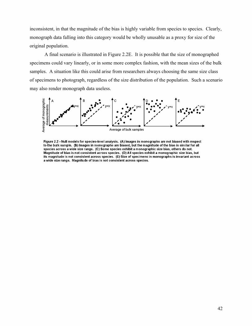
42
inconsistent, in that the magnitude of the bias is highly variable from species to species. Clearly,
monograph data falling into this category would be wholly unusable as a proxy for size of the
original population.
A final scenario is illustrated in Figure 2.2E. It is possible that the size of monographed
specimens could vary linearly, or in some more complex fashion, with the mean sizes of the bulk
samples. A situation like this could arise from researchers always choosing the same size class
of specimens to photograph, regardless of the size distribution of the population. Such a scenario
may also render monograph data useless.

43
RESULTS
Specimen-Level Analysis
The percentile-frequency distributions in Figure 2.3 summarize the results from the
specimen-level analysis. Each group of the data displays a markedly left-skewed distribution,
which indicates that the majority of monograph images in each group have sizes that fall well
above the 50th percentile for a given species’ bulk-collected size-frequency distribution. In fact,
the means of these distributions are tightly constrained between the 65th and 69th percentile (Fig.
2.4; Table 2.2, 1st group). Statistical comparisons of the distributions show no significant
difference in central tendency or distribution shape (Table 2.3).
Species-Level Analysis
Figure 2.5 shows the results of the species-level analysis. In all cases, the scatter plots
resemble the null model for biased yet predictable monographic measurements (Fig. 2.2B),
because the slopes of the least-squares regression lines are close to unity, and the R-squared
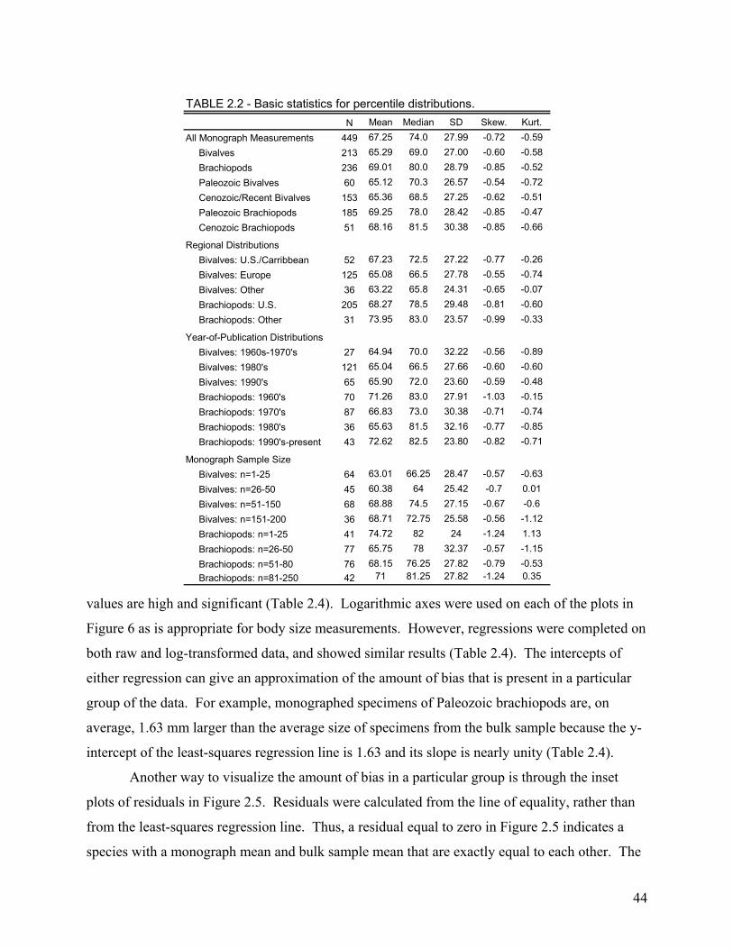
44
N Mean Median SD Skew. Kurt.449 67.25 74.0 27.99 -0.72 -0.59
Bivalves 213 65.29 69.0 27.00 -0.60 -0.58Brachiopods 236 69.01 80.0 28.79 -0.85 -0.52Paleozoic Bivalves 60 65.12 70.3 26.57 -0.54 -0.72Cenozoic/Recent Bivalves 153 65.36 68.5 27.25 -0.62 -0.51Paleozoic Brachiopods 185 69.25 78.0 28.42 -0.85 -0.47Cenozoic Brachiopods 51 68.16 81.5 30.38 -0.85 -0.66
Bivalves: U.S./Carribbean 52 67.23 72.5 27.22 -0.77 -0.26Bivalves: Europe 125 65.08 66.5 27.78 -0.55 -0.74Bivalves: Other 36 63.22 65.8 24.31 -0.65 -0.07Brachiopods: U.S. 205 68.27 78.5 29.48 -0.81 -0.60Brachiopods: Other 31 73.95 83.0 23.57 -0.99 -0.33
Bivalves: 1960s-1970's 27 64.94 70.0 32.22 -0.56 -0.89Bivalves: 1980's 121 65.04 66.5 27.66 -0.60 -0.60Bivalves: 1990's 65 65.90 72.0 23.60 -0.59 -0.48Brachiopods: 1960's 70 71.26 83.0 27.91 -1.03 -0.15Brachiopods: 1970's 87 66.83 73.0 30.38 -0.71 -0.74Brachiopods: 1980's 36 65.63 81.5 32.16 -0.77 -0.85Brachiopods: 1990's-present 43 72.62 82.5 23.80 -0.82 -0.71
Bivalves: n=1-25 64 63.01 66.25 28.47 -0.57 -0.63Bivalves: n=26-50 45 60.38 64 25.42 -0.7 0.01Bivalves: n=51-150 68 68.88 74.5 27.15 -0.67 -0.6Bivalves: n=151-200 36 68.71 72.75 25.58 -0.56 -1.12Brachiopods: n=1-25 41 74.72 82 24 -1.24 1.13Brachiopods: n=26-50 77 65.75 78 32.37 -0.57 -1.15Brachiopods: n=51-80 76 68.15 76.25 27.82 -0.79 -0.53Brachiopods: n=81-250 42 71 81.25 27.82 -1.24 0.35
TABLE 2.2 - Basic statistics for percentile distributions.
Regional Distributions
Year-of-Publication Distributions
Monograph Sample Size
All Monograph Measurements
values are high and significant (Table 2.4). Logarithmic axes were used on each of the plots in
Figure 6 as is appropriate for body size measurements. However, regressions were completed on
both raw and log-transformed data, and showed similar results (Table 2.4). The intercepts of
either regression can give an approximation of the amount of bias that is present in a particular
group of the data. For example, monographed specimens of Paleozoic brachiopods are, on
average, 1.63 mm larger than the average size of specimens from the bulk sample because the y-
intercept of the least-squares regression line is 1.63 and its slope is nearly unity (Table 2.4).
Another way to visualize the amount of bias in a particular group is through the inset
plots of residuals in Figure 2.5. Residuals were calculated from the line of equality, rather than
from the least-squares regression line. Thus, a residual equal to zero in Figure 2.5 indicates a
species with a monograph mean and bulk sample mean that are exactly equal to each other. The
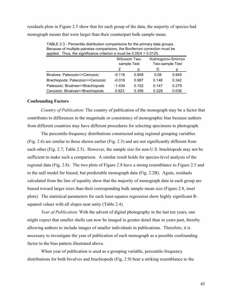
45
residuals plots in Figure 2.5 show that for each group of the data, the majority of species had
monograph means that were larger than their counterpart bulk-sample mean.
Z p D pBivalves: Paleozoic<>Cenozoic -0.116 0.908 0.08 0.945Brachiopods: Paleozoic<>Cenozoic -0.016 0.987 0.148 0.342Paleozoic: Bivalves<>Brachiopods -1.434 0.152 0.147 0.279Cenozoic: Bivalves<>Brachiopods 0.923 0.356 0.229 0.036
Wilcoxon Two-sample Test
Kolmogorov-Smirnov Two-sample Test
TABLE 2.3 - Percentile distribution comparisons for the primary data groups. Because of multiple pairwise comparisons, the Bonferroni correction must be applied. Thus, the significance criterion α must be 0.05/4 = 0.0125.
Confounding Factors
Country of Publication: The country of publication of the monograph may be a factor that
contributes to differences in the magnitude or consistency of monographic bias because authors
from different countries may have different procedures for selecting specimens to photograph.
The percentile-frequency distributions constructed using regional grouping variables
(Fig. 2.6) are similar to those shown earlier (Fig. 2.3) and are not significantly different from
each other (Fig. 2.7; Table 2.5). However, the sample size for non-U.S. brachiopods may not be
sufficient to make such a comparison. A similar result holds for species-level analysis of the
regional data (Fig. 2.8). The two plots of Figure 2.8 have a strong resemblance to Figure 2.5 and
to the null model for biased, but predictable monograph data (Fig. 2.2B). Again, residuals
calculated from the line of equality show that the majority of monograph data in each group are
biased toward larger sizes than their corresponding bulk sample mean size (Figure 2.8, inset
plots). The statistical parameters for each least-squares regression show highly significant R-
squared values with all slopes near unity (Table 2.4).
Year of Publication: With the advent of digital photography in the last ten years, one
might expect that smaller shells can now be imaged in greater detail than in years past, thereby
allowing authors to include images of smaller individuals in publications. Therefore, it is
necessary to investigate the year of publication of each monograph as a possible confounding
factor to the bias pattern illustrated above.
When year of publication is used as a grouping variable, percentile-frequency
distributions for both bivalves and brachiopods (Fig. 2.9) bear a striking resemblance to the
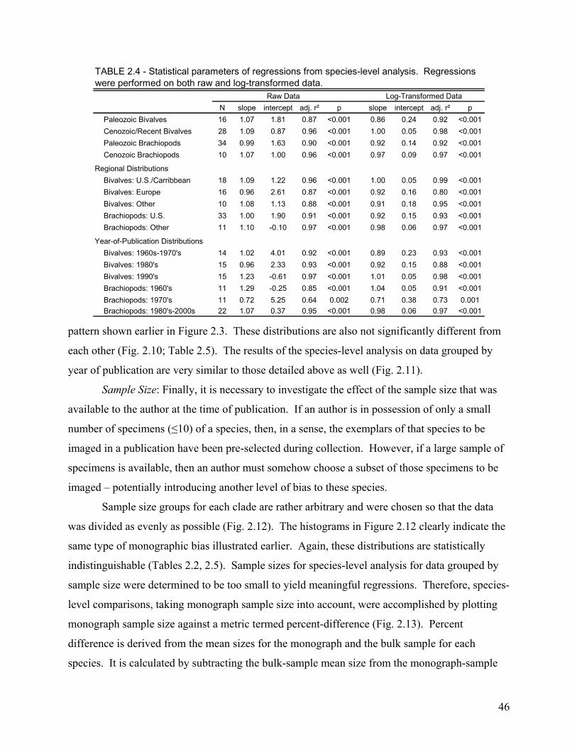
46
N slope intercept adj. r² p slope intercept adj. r² pPaleozoic Bivalves 16 1.07 1.81 0.87 <0.001 0.86 0.24 0.92 <0.001Cenozoic/Recent Bivalves 28 1.09 0.87 0.96 <0.001 1.00 0.05 0.98 <0.001Paleozoic Brachiopods 34 0.99 1.63 0.90 <0.001 0.92 0.14 0.92 <0.001Cenozoic Brachiopods 10 1.07 1.00 0.96 <0.001 0.97 0.09 0.97 <0.001
Bivalves: U.S./Carribbean 18 1.09 1.22 0.96 <0.001 1.00 0.05 0.99 <0.001Bivalves: Europe 16 0.96 2.61 0.87 <0.001 0.92 0.16 0.80 <0.001Bivalves: Other 10 1.08 1.13 0.88 <0.001 0.91 0.18 0.95 <0.001Brachiopods: U.S. 33 1.00 1.90 0.91 <0.001 0.92 0.15 0.93 <0.001Brachiopods: Other 11 1.10 -0.10 0.97 <0.001 0.98 0.06 0.97 <0.001
Bivalves: 1960s-1970's 14 1.02 4.01 0.92 <0.001 0.89 0.23 0.93 <0.001Bivalves: 1980's 15 0.96 2.33 0.93 <0.001 0.92 0.15 0.88 <0.001Bivalves: 1990's 15 1.23 -0.61 0.97 <0.001 1.01 0.05 0.98 <0.001Brachiopods: 1960's 11 1.29 -0.25 0.85 <0.001 1.04 0.05 0.91 <0.001Brachiopods: 1970's 11 0.72 5.25 0.64 0.002 0.71 0.38 0.73 0.001Brachiopods: 1980's-2000s 22 1.07 0.37 0.95 <0.001 0.98 0.06 0.97 <0.001
Log-Transformed Data
TABLE 2.4 - Statistical parameters of regressions from species-level analysis. Regressions were performed on both raw and log-transformed data.
Regional Distributions
Year-of-Publication Distributions
Raw Data
pattern shown earlier in Figure 2.3. These distributions are also not significantly different from
each other (Fig. 2.10; Table 2.5). The results of the species-level analysis on data grouped by
year of publication are very similar to those detailed above as well (Fig. 2.11).
Sample Size: Finally, it is necessary to investigate the effect of the sample size that was
available to the author at the time of publication. If an author is in possession of only a small
number of specimens (≤10) of a species, then, in a sense, the exemplars of that species to be
imaged in a publication have been pre-selected during collection. However, if a large sample of
specimens is available, then an author must somehow choose a subset of those specimens to be
imaged – potentially introducing another level of bias to these species.
Sample size groups for each clade are rather arbitrary and were chosen so that the data
was divided as evenly as possible (Fig. 2.12). The histograms in Figure 2.12 clearly indicate the
same type of monographic bias illustrated earlier. Again, these distributions are statistically
indistinguishable (Tables 2.2, 2.5). Sample sizes for species-level analysis for data grouped by
sample size were determined to be too small to yield meaningful regressions. Therefore, species-
level comparisons, taking monograph sample size into account, were accomplished by plotting
monograph sample size against a metric termed percent-difference (Fig. 2.13). Percent
difference is derived from the mean sizes for the monograph and the bulk sample for each
species. It is calculated by subtracting the bulk-sample mean size from the monograph-sample
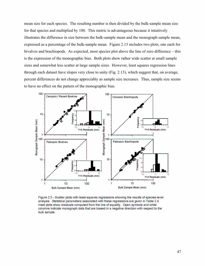
47
mean size for each species. The resulting number is then divided by the bulk-sample mean size
for that species and multiplied by 100. This metric is advantageous because it intuitively
illustrates the difference in size between the bulk-sample mean and the monograph sample mean,
expressed as a percentage of the bulk-sample mean. Figure 2.13 includes two plots, one each for
bivalves and brachiopods. As expected, most species plot above the line of zero difference – this
is the expression of the monographic bias. Both plots show rather wide scatter at small sample
sizes and somewhat less scatter at large sample sizes. However, least squares regression lines
through each dataset have slopes very close to unity (Fig. 2.13), which suggest that, on average,
percent differences do not change appreciably as sample size increases. Thus, sample size seems
to have no effect on the pattern of the monographic bias.
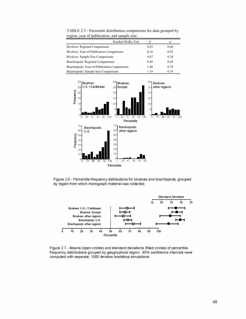
48
Kruskal-Wallis Test χ² pBivalves: Regional Comparisons 0.83 0.66Bivalves: Year-of-Publication Comparisons 0.16 0.92Bivalves: Sample Size Comparisons 4.67 0.20Brachiopods: Regional Comparisons 0.48 0.49Brachiopods: Year-of-Publication Comparisons 1.08 0.78Brachiopods: Sample Size Comparisons 1.19 0.76
TABLE 2.5 - Percentile distribution comparisons for data grouped by region, year of publication, and sample size.
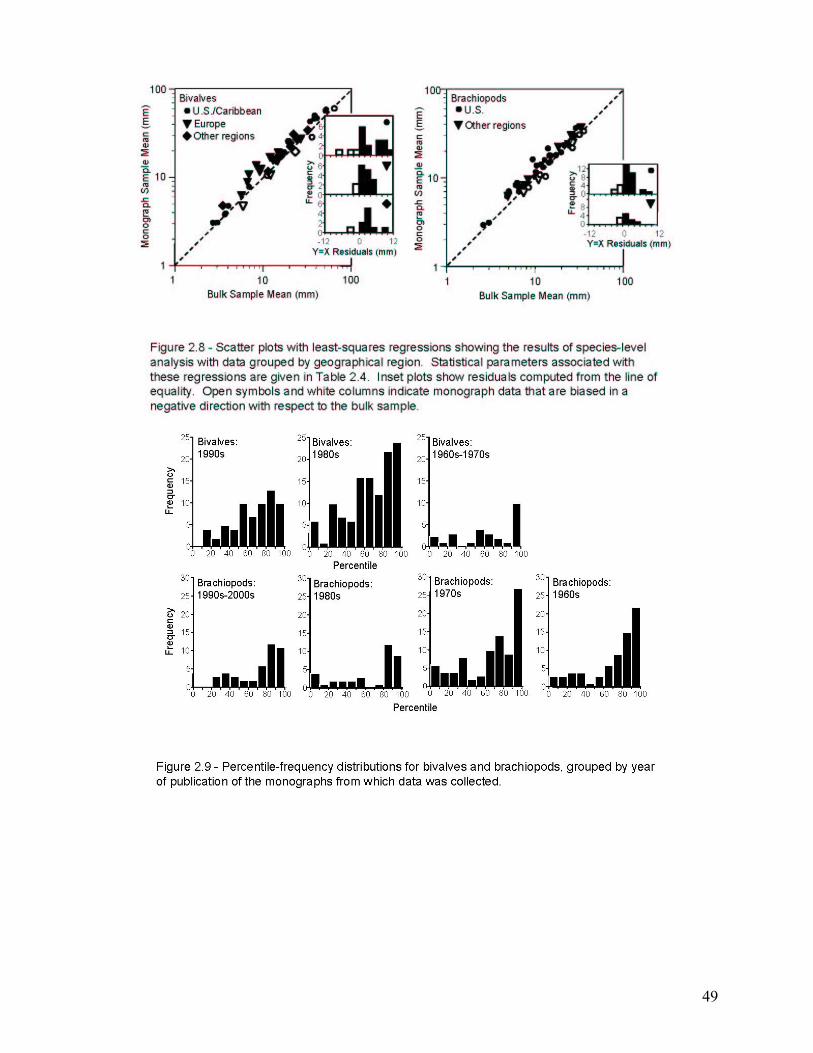
49

50
DISCUSSION
Characterization of the Bias
The principle goal of this paper has been to assess the quality of size measurements from
images in monographs with respect to three parameters: bias direction, bias magnitude, and bias
consistency.
Bias direction and magnitude can be ascertained from the specimen level analysis. The
uniformity of the bias illustrated above is striking (Figs 2.3, 2.4). Authors of monographs seem
to consistently choose a large size-class of specimens for illustration. Even though it may be an

51
inherent human trait to choose large things when presented with a size range (Gould, 1987),
there may be another factor contributing to the bias.
The focus of most monographic studies is alpha-taxonomy. In order to adequately
describe any species, one must first assemble a representative sample of specimens (Mayr et al.,
1953; Blackwelder, 1967). From this sample, a suite of exemplars must then be chosen for
photographic documentation. Intuitively, it is expected that the larger individuals in the sample
would be chosen for this purpose because they often display a full suite of ontogenetic features
that may be useful for species identification, and they may be easier to photograph as well. For
these reasons it is not surprising to see a bias toward larger specimens in the monographic
sample.
Yet, it also seems that authors do not simply choose to image the largest individual
available. If they did, then the magnitude of the bias would be greater. Figure 2.4 indicates that
the means of the percentile-frequency distributions for each data group are constrained to a
narrow interval in the 65th to 69th percentile of the population size-frequency distribution (also
see Table 2.2). Thus, the monographic data used here tended not only to be larger than the mean
of the populations from which they were drawn; they also deviated from this mean by a very
consistent magnitude.
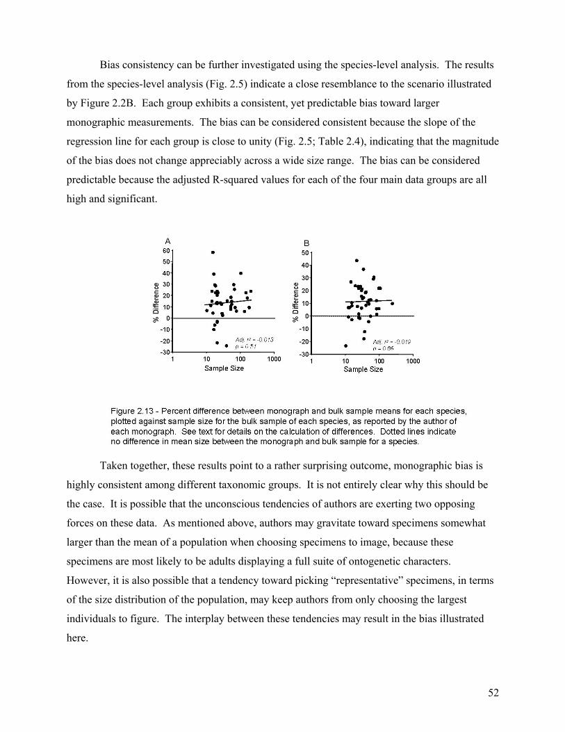
52
Bias consistency can be further investigated using the species-level analysis. The results
from the species-level analysis (Fig. 2.5) indicate a close resemblance to the scenario illustrated
by Figure 2.2B. Each group exhibits a consistent, yet predictable bias toward larger
monographic measurements. The bias can be considered consistent because the slope of the
regression line for each group is close to unity (Fig. 2.5; Table 2.4), indicating that the magnitude
of the bias does not change appreciably across a wide size range. The bias can be considered
predictable because the adjusted R-squared values for each of the four main data groups are all
high and significant.
Taken together, these results point to a rather surprising outcome, monographic bias is
highly consistent among different taxonomic groups. It is not entirely clear why this should be
the case. It is possible that the unconscious tendencies of authors are exerting two opposing
forces on these data. As mentioned above, authors may gravitate toward specimens somewhat
larger than the mean of a population when choosing specimens to image, because these
specimens are most likely to be adults displaying a full suite of ontogenetic characters.
However, it is also possible that a tendency toward picking “representative” specimens, in terms
of the size distribution of the population, may keep authors from only choosing the largest
individuals to figure. The interplay between these tendencies may result in the bias illustrated
here.

53
An Additional Confounding Factor
The results reported above indicate that the potential confounding factors of geography,
year of publication, and sample size, have little effect on the overall pattern of monograph
images yielding consistently larger sizes than bulk-collected specimens of the same species.
However, an issue that has not been addressed is the fact that monograph sample sizes of less
than ten were not included in these analyses so that bulk samples would be sufficiently large to
construct a size-frequency distribution.
It is probable that many monographs feature species for which less than ten specimens
are available. The analyses presented here cannot ascertain whether having very few specimens
to photograph makes any difference to the monographic bias. Figure 2.13 suggests that as
sample size decreases, the range of differences between species’ monograph and bulk sample
increase. Therefore, until the monographic bias for species with small sample size can be
adequately studied, we advocate not using them in literature compilations of body size.
Implications
The highly consistent monographic bias reported here is good news for researchers
interested in collecting meaningful size data from monographs. As long as one is aware of the
presence and nature of bias, it can be taken into account and/or something can be done to correct
for it. For this reason, this study does not advocate a change in the methodology of brachiopod
and bivalve systematists. Furthermore, it can be shown that the monograph sample, though
biased, provides a close approximation to the bulk sample in each case. Thus, relative changes
in size through time ought to be detected equally well by both data types. An illustration of this
point is given in Figure 2.14.
The monograph sample and the bulk sample for each species were compared by grouping
bivalve and brachiopod data into epochs (Fig. 2.14). To construct this comparison, the mean size
for each species was pooled with others from the same epoch. This was done separately for the
monograph sample and the bulk sample. Once pooled by epoch, the mean of these means was
calculated and 95% confidence intervals around this grand mean were computed with separate,
1000-iteration bootstrapping procedures.
These direct comparisons show how well the two datasets (monograph and bulk) track
each other through time for both bivalves and brachiopods (Fig. 2.14). This suggests that even
with a statistically significant bias toward larger specimens in monographs, mean values from the
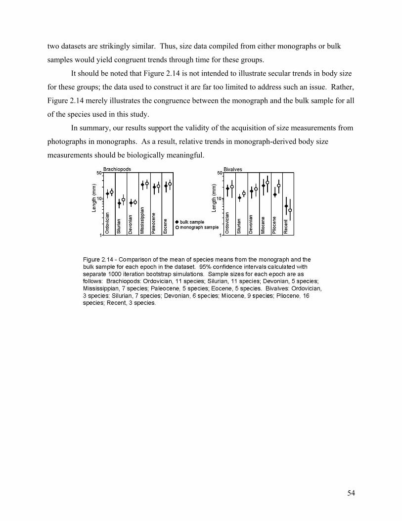
54
two datasets are strikingly similar. Thus, size data compiled from either monographs or bulk
samples would yield congruent trends through time for these groups.
It should be noted that Figure 2.14 is not intended to illustrate secular trends in body size
for these groups; the data used to construct it are far too limited to address such an issue. Rather,
Figure 2.14 merely illustrates the congruence between the monograph and the bulk sample for all
of the species used in this study.
In summary, our results support the validity of the acquisition of size measurements from
photographs in monographs. As a result, relative trends in monograph-derived body size
measurements should be biologically meaningful.

55
CONCLUSIONS
Size measurements of images of specimens in the taxonomic literature can be used to
study body size history. Such measurements represent a biased sample with respect to the mean
size of the population from which they were drawn, but the bias is similar among unrelated
species.
Most specimens studied came from the 65th to 69th percentile of their species’ bulk-
collected size-frequency distribution. This indicates a significant bias toward monograph
specimens that are larger than the mean size of the bulk sample. When compared at the species
level, this bias was found to be highly consistent among the 86 species included in the study.
Thus, size measurements of monographed specimens of bivalves and brachiopods reliably and
consistently record a similar size class for any given species. This is true regardless of
taxonomic affinity, collection locality, and age of the specimens.
The consistency of these results suggests a worker-induced bias that may occur because
of tendencies to choose larger, but not the largest, specimens as exemplars of a species. If this is
the case, then studies of this type on other groups may yield similar results. However, we do not
advocate a change in taxonomic methodologies. The consistency and predictability of the bias
makes it easy to correct for during meta-analyses.
Even when left uncorrected, monograph derived size data closely approximate size trends
exhibited by measurements on bulk-collected specimens. This enables the paleontologist to
utilize two complementary sources of data, so long as they are not mixed in the same analysis.
Field-collected specimens and images in monographs can be used as parallel, independent data
sources in the study of macroevolutionary size trends among major clades. Thus, images of
specimens in monographs represent vast archives of paleoecological information that can, and
should, be used to advance our knowledge of the history of life.
56
CHAPTER THREE1: Comparative time averaging: Age mixing among sympatric bivalves and brachiopods from a modern tropical
shelf
1 This chapter will be submitted for publication to the journal Paleobiology in May 2006. The co-authors for this publication, Susan L. Barbour Wood, Michał Kowalewski, John F. Wehmiller and Marcello G. Simões, contributed less than 20% to the data collection and analysis stages of this project. The text was written completely by R.A. Krause.
57
Abstract
Relatively little is known of how time averaging of marine skeletal accumulations
compares among different species in a single locality. Here we provide quantitative data on the
time averaging magnitude of two species with divergent physical and ecological characteristics,
the terebratellidine brachiopod Bouchardia rosea and the tellinacean bivale Semele casali,
collected from two sites (10 m and 30 m depth) off the coast of Brazil in Ubatuba Bay (Southeast
Brazilian Bight, SW Atlantic). These two species co-occur in large numbers throughout this
tropical mixed carbonate-siliciclastic shelf, and this setting provides a good climatic and
environmental analog to brachiopod- and bivalve-rich shell beds in Paleozoic successions of
North America and Europe.
A total of 161 individual shells were dated using amino acid racemization (D/L aspartic
acid) calibrated with eighteen AMS radiocarbon dates. The dated shells ranged in age from
modern to 12,000 years with a semi-quartile range of 1300 years for brachiopods and 1400 years
for bivalves. The age distributions for each grouping of the data were strongly right-skewed and
dominated by shells less than 3000 years old. The data grouped by species and by site indicates
some significant differences in time averaging magnitude (as measured by the semi-quartile
range). Comparison of brachiopods at the two sites indicates that specimens taken from the 30 m
site are significantly more time averaged than specimens from the 10 m site. No significant
difference is seen in bivalves from the two sites. The most time averaged species from the 10 m
site is S. casali, whereas the most time averaged species from the 30 m site is B. rosea. These
differences among sites are attributed to stochastic variation in the intensity of taphonomic
processes and frequency of exposure at the sediment-water interface. When the data for each
species are pooled, bivalves and brachiopods show very similar time averaging magnitude.
Analysis of the completeness of each sample, using a Monte Carlo model that simulates 100%
complete uniform or exponential distributions, indicates that brachiopods and bivalves were both
likely drawn from 100% complete exponential distributions, although individual sites exhibit
appreciable variation in their putative underlying distributions.
These findings imply an independence of the intrinsic physical characteristics of an
organism and time averaging magnitude, at least among commonly fossilized organisms.
Furthermore, our findings suggest that time averaging magnitude and water depth may be rather
closely related. A meta-analysis of previously published shell ages confirms this pattern for

58
several different latitudes and environments indicating that time averaging magnitude and depth
may have a very similar positive correlation regardless of the depositional system.

59
Introduction
The temporal resolution of the fossil record is an important determinant of the types of
biological and environmental information that can be discerned from the geologic past. It is well
known that most fossiliferous deposits are subject to a suite of postmortem processes that lead to
varying degrees of temporal mixing or time averaging. Since this phenomenon results from the
interaction of many quasi-independent factors, such as physical reworking, transport, and
bioturbation (Martin 1999), the extent of time averaging can be quite variable among different
environments (Kidwell and Bosence 1991; Walker and Voight 1994) and taxa (Kowalewski
1996a, 1997).
The magnitude of time averaging of a fossiliferous deposit is not easily estimated from
the fossil record because dating techniques typically do not provide sufficient resolution,
especially in deposits older than several million years (Brett and Baird 1993; Kidwell 1993).
This problem can be circumvented by using indirect methods such as stratigraphic bracketing
with scattered radiometric dates (Kidwell and Bosence 1991), or by dating shells from modern
sediments and using them as an analog for ancient deposits. The latter method has been used
with increasing frequency in the last decade (Flessa et al. 1993; Wehmiller et al. 1995;
Goodfriend and Stanley 1996; Martin et al. 1996; Anderson et al. 1997; Meldahl et al. 1997;
Flessa 1998; Kowalewski et al. 1998; Carroll et al. 2003; Kidwell et al. 2005), and has yielded
average age ranges of 102-104 yr for marine molluscan assemblages.
Despite this body of work, little is known of time averaging in organisms other than
mollusks (Behrensmeyer et al. 2000; but see Carroll et al. 2003). As a result, it is difficult to
determine how time averaging may vary among sympatric organisms (Martin et al. 1996).
Furthermore, the overprint of different life modes, skeletal mineralogy, and intrinsic durability
on the time averaging signature of organisms is poorly understood. Here we present quantitative
data on comparative time averaging for two sympatric bivalves and brachiopods. We focus on
these organisms because they are common components of the marine biota through much of the
Phanerozoic and one or the other of these taxa have been important contributors to shell beds
since the Ordovician (Kidwell and Brenchley 1996). These two taxa differ markedly in their
mode of life, as well as their skeletal mineralogy. Yet they are often found in similar
environments throughout their stratigraphic ranges. This makes them good candidates for a
comparative study of time averaging.

60
Material for this study was collected from Ubatuba Bay of the Southeast Brazilian Bight
marine province. This area is one of the few places in the world where brachiopods and bivalves
co-occur in appreciable numbers in a sub-tropical, open-shelf setting (Kowalewski et al. 2002;
Simões et al. 2004). As such, this locality provides a unique opportunity to assess the time
averaging characteristics of incipient bivalve and brachiopod shell beds accumulating in an
environment that is closely comparable to Paleozoic shelves.

61
Background
Study Area
Ubatuba Bay, a small embayment located off the coast of the state of São Paulo, Brazil, is
a part of the Southeast Brazilian Bight Marine Province (Campos et al., 1995; Mahiques et al.,
2004). The area is situated at 23° south latitude and is characterized by a humid tropical climate.
Water depths throughout the bay are shallow (0-30 m in the sampled area), salinity is fully
marine (34-35‰), and the mean annual temperature is ~24° C. Oceanographic studies (Campos
et al. 1995, 2000) indicate that the region is dominated by water masses of the South Brazil
Current, a warm west-boundary current flowing from the equator. The area also experiences
seasonal shelf-break upwelling associated with cyclonic meanders of the South Brazil Current,
which bring cold (<20°C) nutrient-rich waters of the South Atlantic Central Water up onto the
inner shelf (Campos et al. 1995, 2000; Braga and Muller 1998). The two sites investigated in
this study are also regularly influenced by the Coastal Water mass and can intermittently
experience fresh-water plumes associated with increased coastal runoff (Campos et al. 1995,
2000).
The sediments of the inner shelf are mixed, but dominated by terrigenous clastics
(~75wt%, Table 3.1). The median grain sizes of these sediments are highly variable, but the
collection sites for this study were dominated by coarse sands and some gravel (Table 3.1). Shell
material, dominated by brachiopods, mollusks, echinoids, bryozoans, and foraminifers, is also
locally abundant and becomes more common toward the outer portions of the bay (Mahiques
1995; Mahiques et al. 1998; Mantelatto and Fransozo 1999; Kowalewski et al. 2002; Simoes et
al. 2004; Barbour Wood et al. in review). Brachiopods and bivalve mollusks are particularly
abundant wherever shell material is present, and two of the most common constituents of the
fauna are the terebratellidine brachiopod Bouchardia rosea, and the tellinacean bivalve Semele
casali.
Bouchardia rosea
The brachiopod used in this study, Bouchardia rosea (Mawe), has a fossil record going
back to the Cretaceous (Mañcenido and Griffin 1988), but is restricted to the Southern
Hemisphere. It is a sessile epifaunal benthic organism that is free lying (Richardson 1981;
Brunton 1996) and inhabits substrates with carbonate concentrations ranging from 40-70%

62
Site Ubatuba 1 Ubatuba 9Depth (meters) 30 m 10 m
Latittude 23° 28' 53" S 23° 26' 41" SLongitude 44° 55' 21" W 45° 02' 07" W
Temperature (°C) 21.2 21.4Salinity (‰) 35 34
Gravel (%) 6.69 24.12Very coarse sand (%) 7.61 14.43Coarse sand (%) 56.63 29.81Medium sand (%) 20.64 18.04Fine sand (%) 4.55 4.81Very fine sand (%) 0.61 1.83Mud (%) 3.28 6.97
Mean diameter (phi) 0.55 0.13Mean diameter (mm) 0.68 0.91Standard deviation 0.91 1.3Skewness -0.27 0.16Kurtosis 4.15 2.34
Sorting (Folk, 1974) moderate poorPercent carbonate 25 25Percent organics 3 7
Table 3.1: Sediment characteristics for the two collection sites.
(Simoes et al. 2004; Kowalewski et al. 2002). Specimens are generally small (<20 mm), but
robust, and are characterized by a low Mg calcite shell that has a punctate fabric. The species is
further characterized by a brachidium with a simple calcareous loop and a strong hinge structure
(Brunton 1996). Like other brachiopods of this order (Terebratulida), the shell of B. rosea is
composed of a thin primary shell layer, a thick, fibrous, secondary shell layer, and lacks a tertiary
layer (Rudwick 1970). The fibrous shell layer is characteristic of extant terebratulides and
rhynchonellides. This feature was also common in Paleozoic members of these groups (Williams
et al. 1997), and was the standard fabric for all spire-bearing brachiopods, pentamerides, and
most orthides (Williams and Rowell, 1965). Thus, the shell structure of B. rosea is very similar
to the type that has been dominant among Rhynchonelliformea throughout the Phanerozoic,
except perhaps during the Permo-Carboniferous (Williams et al. 1997)
Semele casali
The bivalve used in this study, Semele casali, is an infaunal, facultative deposit feeder
that burrows in silt, sand, or mud to a depth of 5 cm, although larger specimens have been

63
recovered from a depth of 11 cm (Narchi and Domaneschi 1977; Domaneschi 1995; Stead et al.
2002). The aragonitic shell is generally small (<20 mm), and thin with weak concentric
sculpture present on the entire external surface of both valves (Narchi and Domaneschi 1977).
Specimens of S. casali have been recovered from the southwestern Atlantic from 20-35° S, and a
depth range of 10-180 m (Narchi and Domaneschi 1977).
The tellinacean genus Semele has a wide distribution in the tropical and temperate oceans
of the northern and southern hemisphere. It is particularly abundant in the eastern Pacific, where
28 species are currently recognized (Coan 1988). The western Atlantic has far fewer extant
species, (only six, including S. casali), but there were far more species in this area in the Tertiary
(Boss 1972; Domaneschi 1995). The Semelidae evolved rather recently, in the Eocene, but the
superfamily Tellinacea has a fossil record going back to the late Triassic. The earliest
representatives were probably very shallow infaunal suspension feeders judging from their lack
of a pallial sinus, but the deeper burrowing habit seen in Semele casali had evolved by the late
Jurassic (Pohlo 1982). Thus, this species represents a shell type and life habit that has been
common throughout most of the Mesozoic and Cenozoic.
Dating Technique
To estimate the scale of time averaging among these two species, we employ here amino
acid racemization (AAR) calibrated with accelerator mass spectrometry (AMS) 14C dating. This
method has been used with increasing frequency in the last several decades because it has proven
reliable and efficient for dating large numbers of specimens (Wehmiller 1982; Miller and Hare
1980; Hearty 1987; Miller et al. 1987; Goodfriend 1987, 1991). It has been applied to a wide
variety of biomineralized fossils and subfossils, including marine organisms (forams, corals,
mollusks, and brachiopods), terrestrial organisms (egg shells, mollusks, plants, bones, teeth), and
other biogenic materials (Goodfriend 1989; Wehmiller et al. 1995; Goodfriend et al. 1996;
Blackwell et al. 2000; Kaufman, 2000; Keil et al. 2000; Kimber and Griffin 2000; Manley et al.
2000; Teece et al. 2000; Waite 2000). In particular, several studies focused on time averaging
rates among marine mollusks and, to a lesser extent, brachiopods have successfully employed
this technique in multiple Holocene, and in some cases Pleistocene environments (Powell and
Davies 1990; Flessa et al. 1993; Flessa and Kowalewski 1994; Wehmiller et al. 1995; Martin et
al. 1996; Meldahl et al. 1997; Kowalewski et al. 1998, 2000; Carroll et al. 2003).

64
Materials and Methods
Sample Collection
Samples were collected as a part of an ongoing project of the marine ecology group of the
São Paulo State University. The collection sites for this study were both on the inner shelf in
Ubatuba Bay (Fig. 3.1). One site was at a depth of 30m meters and was dominated by coarse and
medium grained sands. The other site was in 10m of water and was dominated by coarse sands
and gravel. Samples were collected using a Van Veen grab sampler (1/40 m2), which collects
material from the uppermost several centimeters of the substrate. Brachiopod and bivalve
material were separated, counted and identified to species level for each sample. From each site,
a suite of specimens of the aragonitic bivalve Semele casali (10m: n=36; 30m: n=36), and the
calcitic brachiopod Bouchardia rosea (10m: n=30; 30m: n=28), were chosen randomly from
among all collected specimens for amino acid dating.
Amino Acid Racemization Dating
The age estimate for each shell was obtained by analysis of the amino acid racemization
(AAR) of a single shell fragment. In each case, the shell fragment was taken from the same
location on the shell to minimize intra-shell variability in racemization rate (Goodfriend et al.,
65
1997; Carroll et al., 2003). For brachiopods we sampled the secondary, fibrous shell layer on the
outer margin of each shell directly opposite the hinge, for bivalves, sampling was done near the
outer margin of the shell halfway between the anterior and posterior side. These shell fragments
were then processed according to the procedure outlined by Carroll et al. (2003) and Barbour
Wood et al. (in review), and analyzed for the D and L enantiomers of aspartic acid.
In addition to 129 new shells, we also include here 32 brachiopod shells that were amino
acid dated in an earlier study (Carroll et al. 2003), and were collected from the same 10 m site
that we use in this study. These shells were originally dated using alloisoleucine / isoleucine
(A/I) ratios, but they were reanalyzed for aspartic acid. We found a high positive correlation
between A/I and Asp values for these shells, suggesting that both of these amino acids can be
utilized for dating both mollusks and brachiopods (Barbour Wood et al. in review).
From the 161 shells subjected to AAR analysis, a sub-sample of 18 shells was chosen for
radiocarbon analysis at the NOSAMS Laboratory at Woods Hole Oceanographic Institute. This
sub-sample was chosen non-randomly to maximize the range of D/L Aspartic (Asp) values for
each taxon and site. The absolute ages for this sub-sample of shells were determined using
CALIB (v. 5, Stuvier et al., 2005). The Asp values of the calibrated shells were then used to
determine the ages of the remainder of the sample using the equations below, which are derived
from least-squares regression lines through each data group.
(1) ( )05
6.2
10 1063.40127.0
−×−= AspAge Bouchardia
m
(2) ( )05
6.2
30 1082.30104.0
−×−= AspAge Bouchardia
m
(3) ( )05
041.3
10 1014.11035.1
−
−
××−= AspAgeSemele
m
(4) ( )06
041.3
30 1044.61055.6
−
−
××−= AspAgeSemele
m
The aspartic acid ratio and calculated age for each shell is given in Appendix 3.1. For a
thorough discussion of the calibration of the radiocarbon dates and the derivation of equations 1-
4 refer to Barbour Wood et al. (in review).
Ages calculated using equations 1-4 are subject to the errors involved with the analytical
techniques. The measurement error for aspartic acid can be calculated as the average range in
values for the 2-5 replicates analyzed from each shell fragment. The average range of Asp
values from a single shell in this study is 0.02, which amounts to a measurement error of ~7%

66
using an average Asp value of 0.3. Because this error behaves in a percent-wise rather than an
amount-wise manner, its effects increase with age (Wehmiller and Miller 2000), and when
propagated through the age equations this error can cause age fluctuations in a single shell of
more than 100 years. Thus, to minimize this error, the Asp values used to calculate ages in this
study are the average of all the replicates for each shell. Uncertainties in uncalibrated and
calibrated radiocarbon years were much less than those for amino acid racemization. The
uncertainties for uncalibrated radiocarbon ages (as reported by NOSAMS) ranged from 25 to 90
years and averaged 35 years, while the uncertainties involved with the calibration averaged to 94
years (Barbour Wood et al. in review). Finally, for both species, the range of radiocarbon dates
is less than the total range of the sample. As a result, shell ages calculated to be older than these
radiocarbon-dated shells have a significant amount of uncertainty associated with them.
However, the portion of the dataset affected by this uncertainty is rather small; most of the
calculated shell ages are considered very reliable. Specifically, we are most confident about the
ages for bivalves that are younger than 3000 years (76% of dated bivalves), and brachiopods that
are younger than 7000 years (96% of dated brachiopods).
Quantification and Comparison of Time Averaging
Quantification of time averaging can be accomplished using several different dispersion
metrics. Many previous workers have used the range in ages for a site as an estimate of the
magnitude of time averaging (Flessa et al. 1993; Flessa and Kowalewski 1994; Meldahl et al.
1997). However, range is based on extreme outliers, and is thus particularly sensitive to sample
size. Other studies have used the shell half-life to quantify time averaging (Cummins et al. 1986;
Meldahl et al. 1997). This technique estimates the amount of time needed to remove 50% of the
shells that were initially present, using a best-fit exponential curve for the age-frequency
distribution. The problem is that this method assumes a constant input of shells through the
entire interval and is sensitive to the binning that is used. Other metrics that are commonly used
are the standard deviation (Kowalewski et al. 1998) and the semiquartile range of the age-
frequency distribution for a site (Kidwell et al. 2005).
Here we focus on the semi-quartile range (SQR), but report several other metrics for
comparison with previous studies (Table 3.2). SQR is calculated as the difference between the
fist and third quartile (25th and 75th percentile), divided by two. In other words, SQR is one-half
of the inter-quartile range. It is an intuitive metric because it is reported in the original
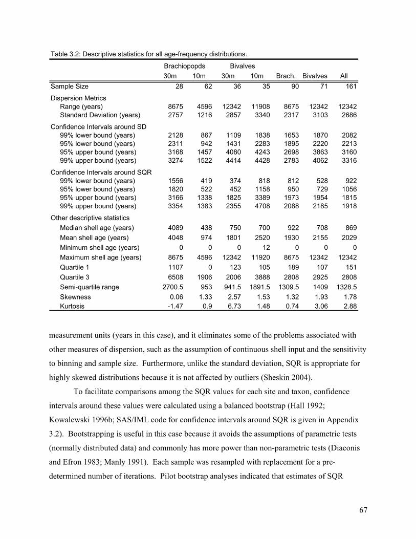
67
30m 10m 30m 10m Brach. Bivalves AllSample Size 28 62 36 35 90 71 161
Dispersion Metrics Range (years) 8675 4596 12342 11908 8675 12342 12342 Standard Deviation (years) 2757 1216 2857 3340 2317 3103 2686
Confidence Intervals around SD 99% lower bound (years) 2128 867 1109 1838 1653 1870 2082 95% lower bound (years) 2311 942 1431 2283 1895 2220 2213 95% upper bound (years) 3168 1457 4080 4243 2698 3863 3160 99% upper bound (years) 3274 1522 4414 4428 2783 4062 3316
Confidence Intervals around SQR 99% lower bound (years) 1556 419 374 818 812 528 922 95% lower bound (years) 1820 522 452 1158 950 729 1056 95% upper bound (years) 3166 1338 1825 3389 1973 1954 1815 99% upper bound (years) 3354 1383 2355 4708 2088 2185 1918
Other descriptive statistics Median shell age (years) 4089 438 750 700 922 708 869 Mean shell age (years) 4048 974 1801 2520 1930 2155 2029 Minimum shell age (years) 0 0 0 12 0 0 0 Maximum shell age (years) 8675 4596 12342 11920 8675 12342 12342 Quartile 1 1107 0 123 105 189 107 151 Quartile 3 6508 1906 2006 3888 2808 2925 2808 Semi-quartile range 2700.5 953 941.5 1891.5 1309.5 1409 1328.5 Skewness 0.06 1.33 2.57 1.53 1.32 1.93 1.78 Kurtosis -1.47 0.9 6.73 1.48 0.74 3.06 2.88
Brachiopopds Bivalves
Table 3.2: Descriptive statistics for all age-frequency distributions.
measurement units (years in this case), and it eliminates some of the problems associated with
other measures of dispersion, such as the assumption of continuous shell input and the sensitivity
to binning and sample size. Furthermore, unlike the standard deviation, SQR is appropriate for
highly skewed distributions because it is not affected by outliers (Sheskin 2004).
To facilitate comparisons among the SQR values for each site and taxon, confidence
intervals around these values were calculated using a balanced bootstrap (Hall 1992;
Kowalewski 1996b; SAS/IML code for confidence intervals around SQR is given in Appendix
3.2). Bootstrapping is useful in this case because it avoids the assumptions of parametric tests
(normally distributed data) and commonly has more power than non-parametric tests (Diaconis
and Efron 1983; Manly 1991). Each sample was resampled with replacement for a pre-
determined number of iterations. Pilot bootstrap analyses indicated that estimates of SQR
68
stabilized after approximately 4000 iterations. Thus, we report here confidence intervals
constructed from 4999 iterations for SQR. In addition, to the random samples, we included in
each case the SQR for the original sample to make 5000 total bootstrap iterations (Manly 1991).
SQR was calculated for each of the bootstrapped samples and the 0.5, 2.5, 97.5, and 99.5
percentiles of the resulting sampling distribution were used to estimate the 95% and 99%
confidence intervals (Efron 1981). For each sample, the bootstrap estimates showed a bias
toward smaller values than the actual SQR. This is a common problem when bootstrapping
dispersion metrics because random samples will often have less variation than the original
sample, but rarely will they have more. To correct for this bias, the mean SQR from each
bootstrap distribution was standardized to value for the original sample (see Kowalewski et al.
1998). The magnitude of this bias was rather variable among the samples (10-200 years) but it
did not affect our interpretations. Thus, more intensive correction methods such as accelerated
bias correction (DiCiccio and Romano 1988) were deemed unnecessary.
Completeness Analysis
The age-frequency distributions obtained in this study can offer insight into the temporal
completeness of the fossil record encompassed by the time averaged samples. This is analogous
to paleontological or stratigraphic completeness (Sadler 1981; Allmon 1989), and can be defined
as the percent of the time intervals, within the time span of a sample, that are represented by a
paleontological record (Kowalewski et al. 1998). The resolution used in this study is 100 years,
because this is the highest resolution that can considered given the accuracy and precision of
amino acid dating and the size and age range of our samples. It is important to note that since
completeness is a scale dependant phenomenon (Sadler 1981); any distribution can appear
complete or incomplete depending on the scale of observation. For example, because of the
chosen resolution for this study, and the size of the samples, it is impossible to obtain a 100%
complete record for three of the four samples considered here (i.e. there are more bins than
specimens). The maximum possible completeness for a sample can be calculated as the sample
size divided by the number of time bins, where the number of time bins is the range of the
sample divided by the resolution (Table 3.3). From these values it is apparent that gaps due to
sampling are inevitable, but it is possible to determine how complete we could expect a sample
to appear, given its size, range, and an assumption of its underlying distribution.

69
30m 10m 30m 10m Brach. Biv. All
Sanple Size 28 62 36 35 90 71 161
Maximum possible completeness (%) 32.2 100 29 29.2 100 57.2 100
Observed completness (%) 27.6 52.2 18.5 16.7 43.7 29 45.2
Uniform distribution (100% complete) Expected completeness (%) 27.8 74.5 25.4 25.6 64.9 43.8 73.1 Confidence intervals around expected 99% lower bound (years) 23.1 63.1 63.1 21 56.5 37.3 65.6 95% lower bound (years) 24.2 65.3 65.3 22.7 57.6 38.9 68.1 95% upper bound (years) 31.1 82.7 82.7 28.6 71.5 47.8 78.6 99% upper bound (years) 32.3 87 87 28.6 73.8 49.4 80.2 Probability of 100% completeness 0.33 0.001 0.001 0.001 0.001 0.001 0.001
Expected completeness (%) 23.2 49.7 21.2 21.5 44.4 32.9 48.6 Confidence intervals around expected 99% lower bound (years) 17.3 37 17 16.8 35.7 25.9 41.3 95% lower bound (years) 18.4 39.2 17.8 18.5 38 28.4 42.9 95% upper bound (years) 27.7 58.7 24.3 25.2 50.7 38.1 54.3 99% upper bound (years) 30 60.9 25.1 26 53 38.9 55.9 Probability of 100% completeness 0.037 0.366 0.052 0.003 0.37 0.043 0.116
Brachiopopds Bivalves
Exponential (right-skewed) distribution (100% complete)
Table 3.3: Results of completeness simulations. See text for discriptions of uniform and exponential distributions.
Completeness analysis (100-year resolution)
With respect to the underlying age-frequency distributions of the samples in this study,
there are two possibilities that will be assessed. First, we will test for what can be conceived as
the best-case scenario for the fossil record, that is, a 100% complete record with uniform and
continuous input of new material in each time interval, and no taphonomic loss of old shells.
Second, we will test for a scenario in which the fossil record is 100% complete, but the chance of
obtaining a paleontological record for a given interval decreases exponentially for each time step.
This is a more realistic scenario because the longer skeletal material is around; the more likely it
is to be removed from the sediment-water interface by burial or the processes of taphonomic
destruction (Kidwell and Bosence 1991; Olszewski 1999, 2004).
We performed seven independent Monte Carlo simulations (one for each sample; one
each for pooled brachiopods and bivalves; one for all of the data) in which we randomly sampled
from 100% complete uniform and exponential distributions (SAS code for these simulations are
in Appendix Three; also see Kowalewski et al. 1998). For each of the four samples, with sample
size k and observed age-range r, we drew k observations from each simulated distribution with a

70
range of r. For each simulation, 999 random samples were generated and their completeness was
calculated at a resolution of 100 years. Again, the addition of the observed completeness value
for each sample yields a sampling distribution of 1000 completeness estimates (Manly 1991),
from which confidence intervals can be calculated from the 0.5, 2.5, 97.5, and 99.5 percentiles.

71
Results
Magnitude and Variation of Time Averaging
The 161 shells dated in this study range in age from 0 (not live collected) to 12342 years,
although 76% of the shells are from the last 3000 years. The age-frequency distribution (AFD)
for all shells (not shown) is strongly right-skewed, with a median shell age of 922 years (Table
3.2). When considered separately, the two species show generally similar patterns. AFDs for
bivalves and brachiopods are each right-skewed (not shown), and their medians, standard
deviations, and semi-quartile ranges are closely comparable (Table 3.2). Consideration of each
site and species separately (Fig. 3.2) indicates that three of the four individual age-frequency
distributions exhibit a strongly right-skewed shape and are significantly different from a normal
distribution (p<0.05, Shapiro-Wilk normality test with Bonferroni correction). The sample that
is not significantly different from a normal distribution is the 30 m brachiopod sample, which has
a platykurtic shape and is multi-modal. As would be expected from the graphical representation
(Fig. 3.2), the 30 m brachiopod sample is significantly different from the other samples in terms
of median age and overall age structure (Kolmogorov-Smirnov and Wilcoxon test, p<0.05). The
other three AFDs are statistically indistinguishable, using the same tests. In addition, the inter-
quartile range for each distribution is shown in Figure 3.2. Each of these ranges overlap, but it is
obvious that the 30 m brachiopod sample is different from the other three.
Variation in time averaging among the samples can be assessed by visual inspection of
the AFDs (Fig. 3.2), and by the analysis of confidence intervals around the SQR values for each
sample (Table 3.2; Figure 3.3). Considering the SQR comparisons in Figure 3.3, the 30 m
bivalve site is the least time averaged sample, followed closely by the 10 m brachiopod site. The
30 m brachiopod site is the most time averaged, and it is significantly different from two of the
sites (10 m brachiopods and 30 m bivalves). Comparisons within each species show a significant
difference in time averaging among the brachiopods sites, and no significant difference among
the bivalve sites. Comparisons between the species indicate that the degree of time averaging for
bivalves and brachiopods at the 30 m site is significantly different, while at the 10 m site the two
species show differences in time averaging, but these differences are not significant. One
complicating factor is that brachiopods are the most time averaged species at the 30 m site, while
bivalves are the most time averaged at the 10 m site. However, when the data for each site is
pooled for each species, the differences in time averaging are no longer apparent. Thus, when
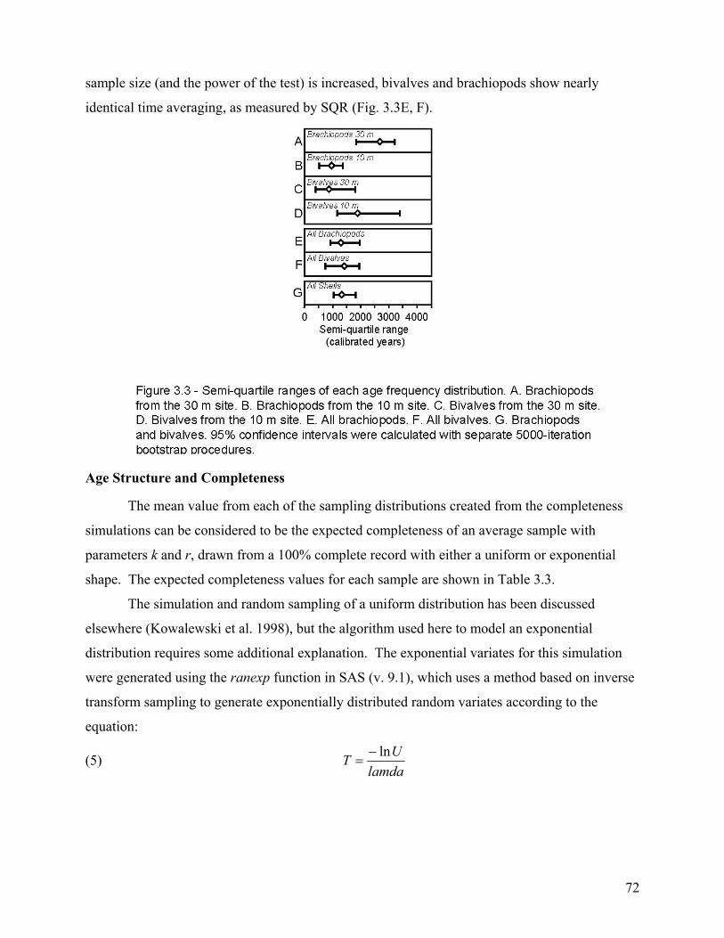
72
sample size (and the power of the test) is increased, bivalves and brachiopods show nearly
identical time averaging, as measured by SQR (Fig. 3.3E, F).
Age Structure and Completeness
The mean value from each of the sampling distributions created from the completeness
simulations can be considered to be the expected completeness of an average sample with
parameters k and r, drawn from a 100% complete record with either a uniform or exponential
shape. The expected completeness values for each sample are shown in Table 3.3.
The simulation and random sampling of a uniform distribution has been discussed
elsewhere (Kowalewski et al. 1998), but the algorithm used here to model an exponential
distribution requires some additional explanation. The exponential variates for this simulation
were generated using the ranexp function in SAS (v. 9.1), which uses a method based on inverse
transform sampling to generate exponentially distributed random variates according to the
equation:
(5) lamda
UT ln−=
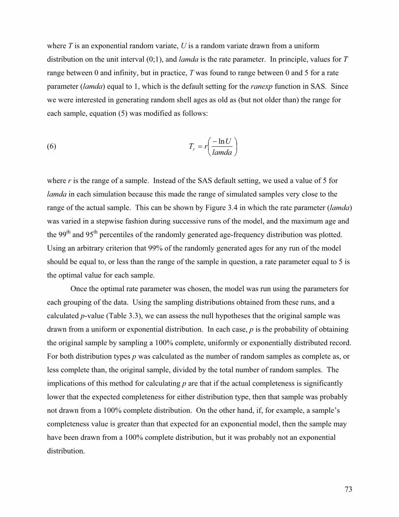
73
where T is an exponential random variate, U is a random variate drawn from a uniform
distribution on the unit interval (0;1), and lamda is the rate parameter. In principle, values for T
range between 0 and infinity, but in practice, T was found to range between 0 and 5 for a rate
parameter (lamda) equal to 1, which is the default setting for the ranexp function in SAS. Since
we were interested in generating random shell ages as old as (but not older than) the range for
each sample, equation (5) was modified as follows:
(6)
−=
lamdaUrTr
ln
where r is the range of a sample. Instead of the SAS default setting, we used a value of 5 for
lamda in each simulation because this made the range of simulated samples very close to the
range of the actual sample. This can be shown by Figure 3.4 in which the rate parameter (lamda)
was varied in a stepwise fashion during successive runs of the model, and the maximum age and
the 99th and 95th percentiles of the randomly generated age-frequency distribution was plotted.
Using an arbitrary criterion that 99% of the randomly generated ages for any run of the model
should be equal to, or less than the range of the sample in question, a rate parameter equal to 5 is
the optimal value for each sample.
Once the optimal rate parameter was chosen, the model was run using the parameters for
each grouping of the data. Using the sampling distributions obtained from these runs, and a
calculated p-value (Table 3.3), we can assess the null hypotheses that the original sample was
drawn from a uniform or exponential distribution. In each case, p is the probability of obtaining
the original sample by sampling a 100% complete, uniformly or exponentially distributed record.
For both distribution types p was calculated as the number of random samples as complete as, or
less complete than, the original sample, divided by the total number of random samples. The
implications of this method for calculating p are that if the actual completeness is significantly
lower that the expected completeness for either distribution type, then that sample was probably
not drawn from a 100% complete distribution. On the other hand, if, for example, a sample’s
completeness value is greater than that expected for an exponential model, then the sample may
have been drawn from a 100% complete distribution, but it was probably not an exponential
distribution.

74
Figure 3.5 shows the modeled completeness values for each distribution type along with
their confidence intervals for each simulation in addition to the observed completeness value for
each sample. From Figure 3.5 it can be seen that one of the samples, the 30 m brachiopod
sample, most closely resembles what would be expected from a 100% complete uniform
distribution (Table 3.3; Fig. 3.5A). Two other samples, the 10 m brachiopod sample and the 30
m bivalve sample, closely resemble the expectation for a 100% complete exponential distribution
(Table 3.3; Fig. 3.5B, C). The completeness value for the fourth sample (10 m bivalve) is lower

75
than what would be expected for either a uniform or an exponentially distributed record (Table
3.3; Fig. 3.5D). The outcome changes somewhat when samples are pooled, as shown in Figure
3.5 E-G. In the case where all shells of a particular species are pooled, the completeness value
for both the brachiopod (Fig. 3.5E) and the bivalve sample (Fig. 3.5F) are consistent with the
expectation for an exponentially distributed record. The same outcome holds when all samples
are pooled (Fig. 3.5G).

76
Discussion and Implications
Comparisons Between the Two Species and Sites
This goal of this study is to quantify and compare the time averaging of bivalves and
brachiopods collected from the same site. These two benthic invertebrate groups are
characterized by many physical differences, each of which could play a role in determining the
type of time averaged assemblage that is produced. The first major difference is skeletal
mineralogy in that (most) bivalves have an aragonitic shell whereas brachiopods are entirely
composed of calcite. This would seem to give brachiopods the advantage in surviving post-
mortem dissolution, as aragonite is unstable relative to calcite in the modern ocean. In fact, early
aragonite dissolution has been implicated in the preferential loss of molluscan material in
Paleozoic (Cherns and Wright 2000), Mesozoic (Hendry et al. 1995, 1996; Wright et al. 2003)
and modern oceans (Morse et al. 1985). Counteracting this effect somewhat is the fact that
brachiopod shells generally have a much higher organic content than bivalves, which may
greatly reduce their durability shortly after the death of the organism (Daley 1993). Shell
microstructure also differs markedly between brachiopods and bivalves. The shell of B. rosea is
punctate with two discrete layers, a thin primary layer composed of fine granular calcite, and a
thick secondary layer composed of fibrous calcite (Rudwick 1970). The shell of S. casali is
composed of several layers of crossed-lamellar aragonite. There has been no detailed
comparative study of these two shell structures, in terms strength or durability, so it is difficult to
assess which of them, if any, would increase the post-mortem survival rate of shells. An
additional physical difference between these species is skeletal robustness or thickness. B. rosea
has a much more robust shell (in terms of thickness) than that of S. casali, and this could imply
that B. rosea is much less susceptible to post-mortem skeletal breakage during transport, but
again, this hypothesis has not been rigorously tested. Finally, these two species differ notably
in their life habit: B. rosea is exclusively epifaunal, while S. casali is primarily a shallow
infaunal organism. These differences in life habit could translate into different time averaging
signatures because infaunal organisms might be more easily buried and less subject to the
physical reworking and transport that can occur at the sediment-water interface.
Their physical differences notwithstanding, we report here that brachiopods and bivalves
can show very similar magnitude of time averaging when collected from the same site or at least
the same region. This suggests that within a single depositional system brachiopods and bivalves
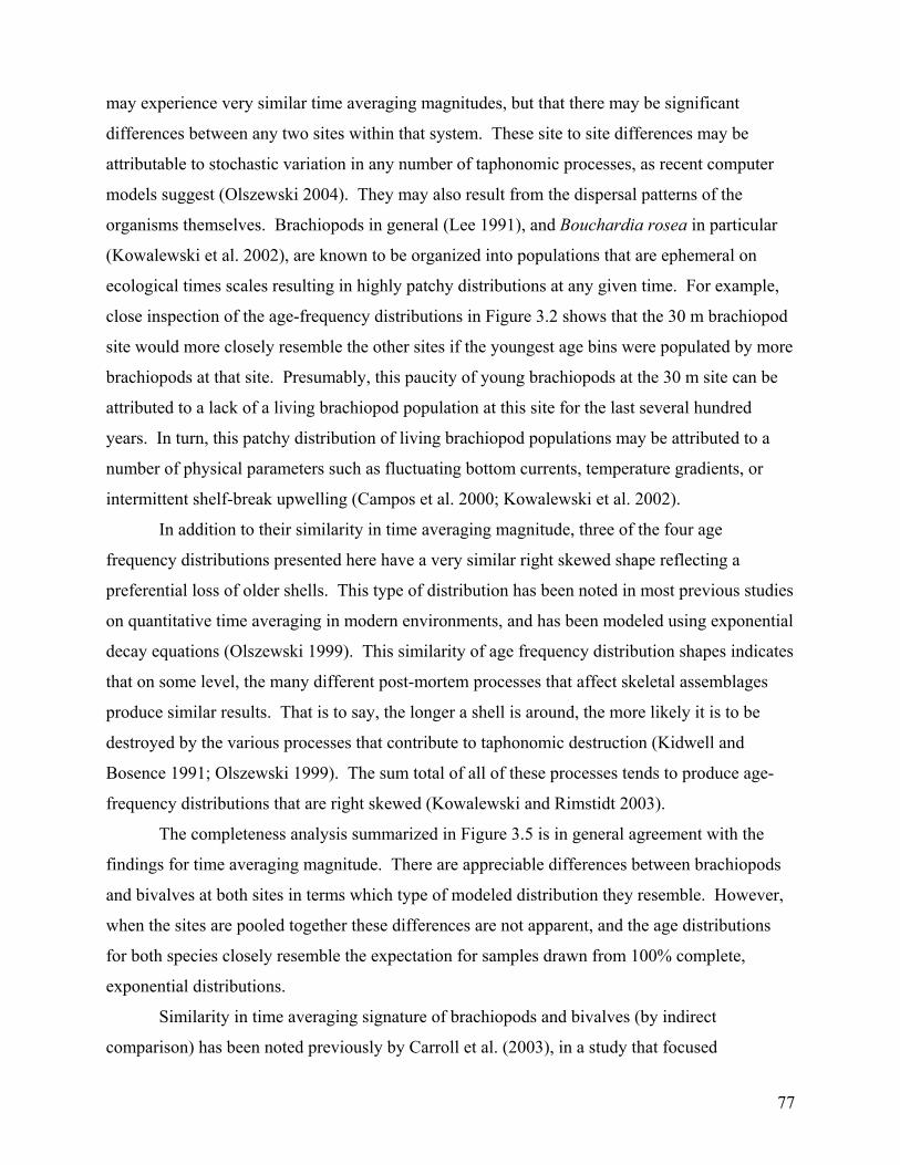
77
may experience very similar time averaging magnitudes, but that there may be significant
differences between any two sites within that system. These site to site differences may be
attributable to stochastic variation in any number of taphonomic processes, as recent computer
models suggest (Olszewski 2004). They may also result from the dispersal patterns of the
organisms themselves. Brachiopods in general (Lee 1991), and Bouchardia rosea in particular
(Kowalewski et al. 2002), are known to be organized into populations that are ephemeral on
ecological times scales resulting in highly patchy distributions at any given time. For example,
close inspection of the age-frequency distributions in Figure 3.2 shows that the 30 m brachiopod
site would more closely resemble the other sites if the youngest age bins were populated by more
brachiopods at that site. Presumably, this paucity of young brachiopods at the 30 m site can be
attributed to a lack of a living brachiopod population at this site for the last several hundred
years. In turn, this patchy distribution of living brachiopod populations may be attributed to a
number of physical parameters such as fluctuating bottom currents, temperature gradients, or
intermittent shelf-break upwelling (Campos et al. 2000; Kowalewski et al. 2002).
In addition to their similarity in time averaging magnitude, three of the four age
frequency distributions presented here have a very similar right skewed shape reflecting a
preferential loss of older shells. This type of distribution has been noted in most previous studies
on quantitative time averaging in modern environments, and has been modeled using exponential
decay equations (Olszewski 1999). This similarity of age frequency distribution shapes indicates
that on some level, the many different post-mortem processes that affect skeletal assemblages
produce similar results. That is to say, the longer a shell is around, the more likely it is to be
destroyed by the various processes that contribute to taphonomic destruction (Kidwell and
Bosence 1991; Olszewski 1999). The sum total of all of these processes tends to produce age-
frequency distributions that are right skewed (Kowalewski and Rimstidt 2003).
The completeness analysis summarized in Figure 3.5 is in general agreement with the
findings for time averaging magnitude. There are appreciable differences between brachiopods
and bivalves at both sites in terms which type of modeled distribution they resemble. However,
when the sites are pooled together these differences are not apparent, and the age distributions
for both species closely resemble the expectation for samples drawn from 100% complete,
exponential distributions.
Similarity in time averaging signature of brachiopods and bivalves (by indirect
comparison) has been noted previously by Carroll et al. (2003), in a study that focused

78
exclusively on B. rosea. This result is contradictory to several recent taphonomic reviews
(Kidwell and Bosence 1991; Kowalewski 1996; Martin 1999; Behrensmeyer et al. 2000), all of
which emphasize the potential impact of intrinsic skeletal characteristics on patterns of time
averaging. However, in a recent study, Behrensmeyer et al. (2005) showed that of the common
shell-producing taxa in the fossil record (bivalves, brachiopods, gastropods), the most common
genera are just as likely to be small, thin shelled, and unreinforced as large, thick shelled, and
ribbed or folded. To the extent that commonness can indicate a high rate of post-mortem skeletal
survivability, this implies that intrinsic shell characteristics and susceptibility to taphonomic
destruction may be independent for these groups.
This similarity of time averaging signature between two different organisms has
important implications for some of the negative aspects of time averaging including the
reduction of the temporal resolution of the fossil record (i.e. Fursich and Aberhan 1990), and the
generation of false patterns (i.e. Wilson 1988; Kowalewski 1996a; Bush et al. 2002). The
analyses presented here agree with many previous studies focused on the quantification of time
averaging patterns in that even single samples, collected to minimize their stratigraphic and
temporal span, may be significantly time averaged (Kowalewski et al. 1998). However, it is
encouraging to note that this pattern seems to be a general one that does not vary appreciably
between different shell-producing species. Thus, the temporal resolution of multi-taxic shell
assemblages in the fossil record may depend more on environmental and taphonomic factors
than it does on the intrinsic properties of their component organisms. Furthermore, since
intrinsic durability seems to play a minor role in dictating the formation of a fossil assemblage,
the fidelity of the fossil record with respect to biological parameters such as diversity,
morphology and size structure may be rather good, even for less durable shell-producers, as has
recently been suggested (Bush et al. 2002; Kowalewski et al. 2003; Krause 2004; Tomasovych
2004).
Comparisons with other regions
The estimates of time averaging presented here are of the same order of magnitude as
those reported in other recent empirical studies of time averaging duration for shelled marine
invertebrates (Flessa et al. 1993; Meldahl et al. 1997; Kowalewski et al. 1998; Carroll et al.
2003; Kidwell et al. 2005). However, the time averaging durations reported here using SQR are
consistently greater than most other studies. One of the reasons for this could be the fact that
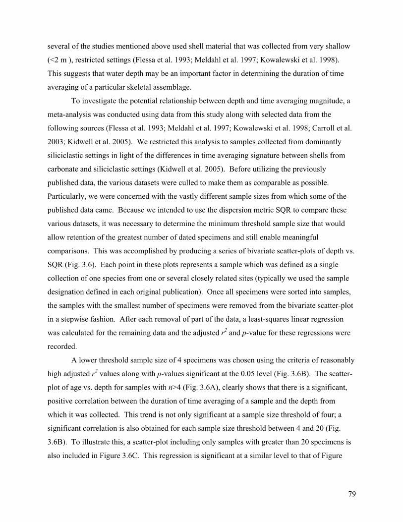
79
several of the studies mentioned above used shell material that was collected from very shallow
(<2 m ), restricted settings (Flessa et al. 1993; Meldahl et al. 1997; Kowalewski et al. 1998).
This suggests that water depth may be an important factor in determining the duration of time
averaging of a particular skeletal assemblage.
To investigate the potential relationship between depth and time averaging magnitude, a
meta-analysis was conducted using data from this study along with selected data from the
following sources (Flessa et al. 1993; Meldahl et al. 1997; Kowalewski et al. 1998; Carroll et al.
2003; Kidwell et al. 2005). We restricted this analysis to samples collected from dominantly
siliciclastic settings in light of the differences in time averaging signature between shells from
carbonate and siliciclastic settings (Kidwell et al. 2005). Before utilizing the previously
published data, the various datasets were culled to make them as comparable as possible.
Particularly, we were concerned with the vastly different sample sizes from which some of the
published data came. Because we intended to use the dispersion metric SQR to compare these
various datasets, it was necessary to determine the minimum threshold sample size that would
allow retention of the greatest number of dated specimens and still enable meaningful
comparisons. This was accomplished by producing a series of bivariate scatter-plots of depth vs.
SQR (Fig. 3.6). Each point in these plots represents a sample which was defined as a single
collection of one species from one or several closely related sites (typically we used the sample
designation defined in each original publication). Once all specimens were sorted into samples,
the samples with the smallest number of specimens were removed from the bivariate scatter-plot
in a stepwise fashion. After each removal of part of the data, a least-squares linear regression
was calculated for the remaining data and the adjusted r2 and p-value for these regressions were
recorded.
A lower threshold sample size of 4 specimens was chosen using the criteria of reasonably
high adjusted r2 values along with p-values significant at the 0.05 level (Fig. 3.6B). The scatter-
plot of age vs. depth for samples with n>4 (Fig. 3.6A), clearly shows that there is a significant,
positive correlation between the duration of time averaging of a sample and the depth from
which it was collected. This trend is not only significant at a sample size threshold of four; a
significant correlation is also obtained for each sample size threshold between 4 and 20 (Fig.
3.6B). To illustrate this, a scatter-plot including only samples with greater than 20 specimens is
also included in Figure 3.6C. This regression is significant at a similar level to that of Figure
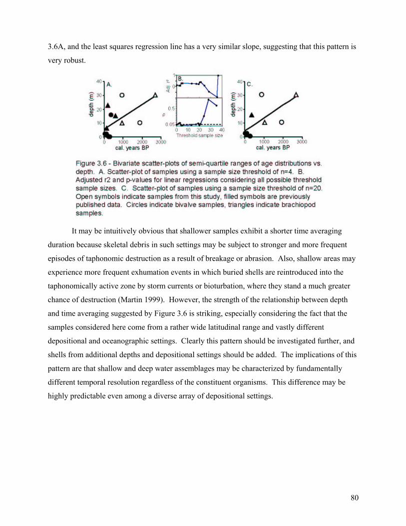
80
3.6A, and the least squares regression line has a very similar slope, suggesting that this pattern is
very robust.
It may be intuitively obvious that shallower samples exhibit a shorter time averaging
duration because skeletal debris in such settings may be subject to stronger and more frequent
episodes of taphonomic destruction as a result of breakage or abrasion. Also, shallow areas may
experience more frequent exhumation events in which buried shells are reintroduced into the
taphonomically active zone by storm currents or bioturbation, where they stand a much greater
chance of destruction (Martin 1999). However, the strength of the relationship between depth
and time averaging suggested by Figure 3.6 is striking, especially considering the fact that the
samples considered here come from a rather wide latitudinal range and vastly different
depositional and oceanographic settings. Clearly this pattern should be investigated further, and
shells from additional depths and depositional settings should be added. The implications of this
pattern are that shallow and deep water assemblages may be characterized by fundamentally
different temporal resolution regardless of the constituent organisms. This difference may be
highly predictable even among a diverse array of depositional settings.
81
Conclusions
1. Brachiopods and bivalves have a similar time averaging signature when collected from the
same depositional setting. This similarity is present when a variety of different metrics are
considered, including standard deviation, semi-quartile range and overall shape of the age-
frequency distribution.
2. Extrinsic factors such as environment and depth are more important than intrinsic factors such
as shell mineralogy, durability, and life habit in determining time averaging magnitude. As a
result, the temporal resolution of the fossil record of inherently less durable shell-producing
taxa may be much more closely comparable with that of durable taxa than has previously
been appreciated.
3. Results of simulations of temporal completeness suggest that shell accumulations from open
marine environments may be drawn from underlying distributions that are indistinguishable
from 100% complete records. The shapes of these distributions are dictated by the
population dynamics for the organism over the time averaged interval, but they need not
conform to a simple exponential model. This explains why very old shells can be relatively
common at some sites.
4. There is a significant relationship between the time averaging duration of a skeletal
assemblage and the water depth at which it accumulated. Deeper assemblages are more
likely to have longer time averaging duration than shallow assemblages perhaps because of
the increased intensity and frequency of episodes of taphonomic destruction at shallow
depths.

82
REFERENCES
ADRAIN, J. M. 2001. Systematic paleontology: Journal of Paleontology 75: 1055-1057. ALBERSTADT, L. P. 1979. The brachiopod genus Platystrophia: U S Geological Survey
Professional Paper, Report: P 1066 B, p. B1-B20. ALEXANDER, R.R. 1990. Mechanical strength of shells of selected extant articulate brachiopods:
implications for Paleozoic morphologic trends: Historical Biology 3: 169-188. ALLMON, W. D. 1989. Paleontological completeness of the record of lower Tertiary mollusks,
U.S. Gulf and Atlantic Coastal Plains: implications for phylogenetic studies. Historical Biology 3:141-158.
ALROY, J., C. R. MARSHALL, R. K. BAMBACH, K. BEZUSKO, M. FOOTE, F. T. FURSICH, T. A.
HANSEN, S. M. HOLLAND, L. C. IVANY, D. JABLONSKI, D. K. JACOBS, M. A. KOSNIK, S. LIDGARD, S. LOW, A. I. MILLER, P. M. NOVACK-GOTTSHALL, T. D. OLSZEWSKI, M. E. PATZKOWSKY, D. M. RAUP, K. ROY, J. J. SEPKOSKI, JR., M. G. SOMMERS, P. J. WAGNER, AND A. WEBBER. 2001. Effects of sampling standardization on estimates of Phanerozoic marine diversification. Proceedings of the National Academy of Sciences 98(11):6261-6266.
AMANO, K. 1986. Age and characteristics of the so-called "Atsunai-Togeshita Fauna" in
Hokkaido: in T. Kotaka, eds., Japanese Cenozoic Molluscs: Their origin and migration. Paleontological Society of Japan, p. 187-198.
AMSDEN, T. W. 1968. Articulate brachiopods of the St. Clair Limestone (Silurian), Arkansas, and
the Clarita Formation (Silurian), Oklahoma. Memoir 1, Paleontological Society, 117 p. ANDERSON, L.C., B.K. SEN GUPTA, R.A. MCBRIDE, AND M.R. BYRNES. 1997. Reduced
seasonality of Holocene climate and pervasive mixing of Holocene marine section: Northeastern Gulf of Mexico shelf. Geology 25: 127-130.
BABIN, C. AND M. MELOU. 1972. Mollusques Bivalves et Brachiopodes des "schistes de
Raguenez" (Ordovicien superieur du Finistere); consequences stratigraphiques et paleobiogeographiques. Bivalve mollusks and brachiopods of the Raguenez Shale (Upper Ordovician of Finistere); stratigraphic and paleobiogeographic consequences. Annales - Societe Geologique du Nord 92: 79-93.
BALINSKI, A. 1995. Devonian athyridoid brachiopods with double spiralia. Acta Palaeontologica
Polonica 40: 129-148. BALINSKI, A. 1997. A new atrypid genus (Brachiopoda) from the Frasnian of Poland. Acta
Palaeontologica Polonica 42: 427-435.
83
BAMBACH, R. K. 1977. Species richness in marine benthic habitats through the Phanerozoic. Paleobiology 3: 152-167.
BARBOUR WOOD, S.L., R. A. KRAUSE JR., M. KOWALEWSKI, J. F. WEHMILLER, M. G. SIMÕES,
AND G. A. GOODFRIEND. 2003. A comparison of rates of time averaging between the bivalve Macoma cleryana and brachiopod Bouchardia rosea on a shallow subtropical shelf: Geological Society of America, Abstracts with Programs v. 35, no. 6.
BARBOUR WOOD, S. L., R. A. KRAUSE JR., M. KOWALEWSKI, J. F. WEHMILLER, AND M. G.
SIMÕES. In review. Aspartic acid racemization dating of Holocene brachiopods and bivalves from the Southern Brazilian Shelf, South Atlantic. Quaternary Research.
BEHRENSMEYER, A. K., AND S. M. KIDWELL. 1985. Taphonomy's contributions to paleobiology.
Paleobiology 11:105-119. BEHRENSMEYER, A.K., S. M. KIDWELL AND R. A. GASTALDO. 2000. Taphonomy and
paleobiology, in Erwin, D.H., and Wing, S.L., eds., Deep Time: Paleobiology's Perspective: The Paleontological Society, p. 103-147.
BEHRENSMEYER, A. K., F. T. FURSICH, R. A. GASTALDO, S. M. KIDWELL, M. A. KOSNIK, M.
KOWALEWSKI, R. E. PLOTNICK, R. R. ROGERS, AND J. ALROY. 2005. Are the most durable shelly taxa also the most common in the marine fossil record? Paleobiology 31(4):607-623.
BELL, M.A., M. S. SADAGURSKY, J. V. BAUMGARTNER. 1987. Utility of lacustrine deposits for the
study of variation within fossil assemblages. Palaios 2: 455-466. BENTON, M. J. 1993. The fossil record 2. London, Chapman & Hall BIRD, S. O. 1965. Upper Tertiary Arcacea of the Mid-Atlantic coastal plain. Paleontographica
Americana 5: 1-62. BLACKWELDER, R. E. 1967. Taxonomy, a text and reference book, New York, John Wiley &
Sons, Inc., 698 p. BLACKWELL, B. A. B., W. M. LAST AND N. W. RUTTER. 2000. Biogeochemical diagenesis in
recent mammalian bones from saline lakes in western Victoria, Australia. In: Goodfriend, G. A., Collins, M. J., Fogel, M. L., Macko, S. A., and Wehmiller, J. F. (Eds.), Perspectives in Amino Acid and Protein Geochemistry. Oxford University Press, pp. 88-107.
BOOKSTEIN, F.L. 1990. Introduction to methods for landmark data, in Rohlf, F.J., and Bookstein,
F.L., eds., Proceedings of the Michigan morphometrics workshop: University of Michigan Museum of Zoology.
BOOKSTEIN, F.L. 1991. Morphometric tools for landmark data: geometry and biology:
Cambridge University Press, 435 p.
84
BOOKSTEIN, F.L. 1996. Combining the tools of geometric morphometrics in Marcus, L.F., Corti,
M., Loy, A., Naylor, G.J.P., and Slice, D.E., eds., Advances in Morphometrics: NATO ASI Series A: Life Sciences vol. 284, p.131-151.
BOSS, K. J. 1972. The genus Semele in the Western Atlantic. Johnsonia 5(49):1-32. BRAGA, E. S., AND T. J. MULLER. 1998. Observation of regeneration of nitrate, phosphate and
silicate during upwelling off Ubatuba, Brazil, 23 degrees south. Continental Shelf Research 18:915-922.
BRETT, C. E., AND G. C. BAIRD. 1993. Taphonomic approaches to temporal resolution in
stratigraphy: Examples from Paleozoic marine mudrocks. Pp. 250-274. In S. M. Kidwell, and A. K. Behrensmeyer, eds. Taphonomic approaches to time resolution in fossil assemblages. The Paleontological Society.
BRUNTON, C. H. C. 1996. The functional morphology of the Recent brachiopod Bouchardia
rosea. Acta Zoologica 77:233-240. BUSH, A.M., M. G. POWELL, W. S. ARNOLD, T. M. BERT, AND G. M. DALEY. 2002. Time
averaging, evolution, and morphologic variation. Paleobiology 28: 9-25. BUTLER, J. B., S. N. LANE, AND J. H. CHANDLER. 2001. Automated extraction of grain-size data
from gravel surfaces using digital image processing. Journal of Hydraulic Research 39(5):519-529.
CAMPOS, E. J. D., D. VELHOT, AND I. C. A. DA SILVEIRA. 2000. Shelf break upwelling driven by
Brazil Current cyclonic meanders. Geophysical Research Letters 27:751-754. CARROLL, M., M. KOWALEWSKI, M. G. SIMOES, AND G. A. GOODFRIEND. 2003. Quantitative
estimates of time-averaging in brachiopod shell accummulations from a modern tropical shelf. Paleobiology 29(3):381-402.
CHAPMAN, R. E. 1990. Conventional Procrustes Approaches. In F. J. Rohlf, and F. L. Bookstein,
eds. Proceedings of the Michigan morphometrics workshop. University of Michigan Museum of Zoology.
CHERNS, L. AND V. P. WRIGHT. 2000. Missing mollusks as evidence of large-scale, early skeletal
aragonite dissolution in a Silurian sea. Geology 28: 791-794. COAN, E. V. 1988. Recent eastern Pacific species of the bivalve genus Semele. The Veliger 31:1-
42. COOPER, G. A. 1988. Some Tertiary brachiopods of the East Coast of the United States.
Smithsonian Contributions to Paleobiology 64:1-45.

85
CRAIG, R. S. 2000. The Cenozoic brachiopods of the Carnarvon Basin, Western Australia. Palaeontology 43: 111-152.
CUMMINS, H., E. N. POWELL, J. STANTON, ROBERT J., AND G. M. STAFF. 1986. The rate of
taphonomic loss in modern benthis habitats: how much of the potentially preservable community is preserved? Palaeogeography Palaeoclimatology Palaeoecology 89:193-204.
DALEY, G. M. 1993. Passive deterioration of shelly material: A study of the Recent Eastern
Pacific articulate brachiopod Terebratalia transversa. Palaios 8:226-232. DIACONIS, P., AND B. EFRON. 1983. Computer intensive methods in statistics. Scientific
American 248:116-130. DICICCIO, T. J., AND J. P. ROMANO. 1988. A review of bootstrap confidence intervals. Journal of
the Royal Statistical Society B (Methodological) 50:338-354. DOMANESCHI, O. 1995. A comparative study of the functional morphology of Semele
purpurascens (Gmelin, 1791) and Semele proficua. The Veliger 38(4):323-342. DRYDEN, I. L., AND K. V. MARDIA. 1998. Statistical shape analysis. John Wiley and sons. DU BOIS, H. M. 1916. Variation induced in brachiopods by environmental conditions. Puget
Sound Marine Station Publications 1(16):177-183. EFREMOV, J. A. 1940. Taphonomy: a new branch of paleontology. Pan-American Geologist 74:
81-93 EFRON, B. 1981. Nonparametric standard errors and confidence intervals. Canadian Journal of
Statistics 9:139-172. FLESSA, K. W. 1998. Well-traveled cockles: Shell transport during the Holocene transgression of
the southern North Sea. Geology 26: 187-190. FLESSA, K. W., A. H. CUTLER, AND K. H. MELDAHL. 1993. Time and taphonomy: quantitative
estimates of time -averaging and stratigraphic disorder in a shallow marine habitat. Paleobiology 19(2):266-286.
FLESSA, K. W., AND M. KOWALEWSKI. 1994. Shell survival and time averaging in nearshore and
shelf environments: estimates from the radiocarbon literature. Lethaia 27:153-165. FURSICH, F. T., AND M. ABERHAN. 1990. Significance of time averaging for paleocommunity
analysis. Lethaia 23:143-152. GOODFRIEND, G. A., 1987. Chronostratigraphic studies of sediments in the Negev Desert, using
amino acid epimerization analysis of land snail shells. Quaternary Research 28: 374-392.

86
GOODFRIEND, G. A., 1989. Complementary use of amino acid epimerization and radiocarbon analysis for dating mixed-age fossil assemblages. Radiocarbon 31: 1041-1047.
GOODFRIEND, G. A., 1992. Rapid racemization of aspartic acid in mollusc shells and potential for
dating over Recent centuries. Nature 357: 399-401. GOODFRIEND, G. A., J. BRIGHAM-GRETTE AND G. H. MILLER. 1996. Enhanced age resolution of
the marine Quaternary record in the Arctic using aspartic acid racemization dating of bivalve shells. Quaternary Research 45: 176-187.
GOODFRIEND, G. A., K. W. FLESSA AND P. H. HARE. 1997. Variation in amino acid epimerization
rates and amino acid composition among shell layers in the bivalve Chione from the Gulf of California. Geochimica et Cosmochimica Acta 61, 1487-1493.
GORDON, M., JR., T. W. HENRY, AND J. D. TREWORGY. 1993. Late Mississppian productoid
brachiopods Inflatia, Keokukia, and Adairia, Ozark region of Oklahoma and Arkansas. Memoir - Paleontological Society 30:29.
GOULD, S. J. 1987. Cope's rule as psychological artefact. Nature 385:189-190. HALL, P. 1992. Efficient bootstrap simulations. Pp. 127-143. In R. Lepage, and L. L. Billard, eds.
Exploring the limits of bootstrap. Wiley, New York. HEARTY, P. J. 1987. New data on the Pleistocene of Mallorca. Quaternary Science Reviews 6:
245-257. HENDRY, J. P., P. W. DITCHFIELD AND J. D. MARSHALL. 1995. Two stage metamorphism of
Jurassic aragonitic bivalves: Implications for early diagenesis. Journal of Sedimentary Research A65: 214-224.
HENDRY, J. P., N. H. TREWIN AND A. E. FALLICK. 1996. Low Mg-calcite marine cement in
Cretaceous turbidites: Origin, spatial distribution, and relationship to sea-water chemistry. Sedimentology 43: 877-900.
HOWE, H. J. 1979. Middle and Late Ordovician plectambonitacean, rhynchonellacean,
syntrophiacean, trimerellacean, and atrypacean brachiopods: U S Geological Survey Professional Paper, Report: P 1066 C, p. C1-C18.
IBBEKEN, H. AND R. SCHLEYER. 1986. Photo-sieving: A method for grain size analysis of coarse-
grained, unconsolidated bedding surfaces. Earth Surface Processes and Landforms 11: 59-77.
JOHNSTON, P. A. 1993. Lower Devonian Pelecypoda from southeastern Australia: Memoir 14 -
Association of Australasian Paleontologists, p. 1-134.
87
JUNG, P. 1996. Neogene paleontology in the northern Dominican Republic; 17, The families Cuspidariidae and Verticordiidae (Mollusca, Bivalvia). Bulletins of American Paleontology 110: 35-75.
KAUFMAN, D. S., 2000. Amino acid racemization in ostracodes. In: Goodfriend, G. A., Collins,
M. J., Fogel, M. L., Macko, S. A., and Wehmiller, J. F. (Eds.), Perspectives in Amino Acid and Protein Geochemistry. Oxford University Press, pp. 145-160.
KEIL, R. G., E. TSAMAKIS, AND J. I. HEDGES. 2000. Early diagenesis of particulate amino acids in
marine systems. In: Goodfriend, G. A., Collins, M. J., Fogel, M. L., Macko, S. A., and Wehmiller, J. F. (Eds.), Perspectives in Amino Acid and Protein Geochemistry. Oxford University Press, pp. 69-82.
KIDWELL, S. M. 1986. Models for fossil concentrations: paleobiologic implications. Paleobiology
12(2):6-24. KIDWELL, S. M. 1993. Patterns of time averaging in the shallow marine fossil record. Pp. 275-
300. In S. M. Kidwell, and A. K. Behrensmeyer, eds. Taphonomic approaches to time resolution in fossil assemblages. Short Courses in Paleontology 6. Paleontological Society.
KIDWELL, S. M., AND D. W. J. BOSENCE. 1991. Taphonomy and time-averaging of marine shelly
faunas. Pp. 116-188. In P. A. Allison, and D. E. G. Briggs, eds. Taphonomy: Releasing the data locked in the fossil record. Plenum Press.
KIDWELL, S. M., AND P. BRENCHLEY. 1994. Patterns in bioclastic accumulation through the
Phanerozoic: Changes in input or in destruction? Geology 22:1139-1143. KIDWELL, S. M., AND P. J. BRENCHLEY. 1996. Evolution of the fossil record: Thickness trends in
marine skeletal accumulations and their implications. Pp. 290-336. In D. Jablonski, D. H. Erwin, and J. H. Lipps, eds. Evolutionary Paleobiology. University of Chicago Press.
KIDWELL, S. M., M. M. R. BEST, AND D. S. KAUFMAN. 2005. Taphonomic trade-offs in tropical
marine death assemblages: Differential time averaging, shell loss, and probable bias in siliciclastic vs. carbonate facies. Geology 33: 729-732.
KIMBER, R. W. L., AND C. V. GRIFFIN. 2000. Interpretation of D/L amino acid data from
agricultural soils. In: Goodfriend, G. A., Collins, M. J., Fogel, M. L., Macko, S. A., and Wehmiller, J. F. (Eds.), Perspectives in Amino Acid and Protein Geochemistry. Oxford University Press, pp. 195-201.
KOWALEWSKI, M. 1996a. Time-averaging, Overcompleteness, and the Geological Record.
Journal of Geology 104:317-326. KOWALEWSKI, M. 1996b. Taphonomy of a Living Fossil: The Lingulide Brachiopod Glottidia
palmeri Dall from Baja California, Mexico. Palaios 11:244-265.
88
KOWALEWSKI, M. 1997. The Reciprocal Taphonomic Model. Lethaia 30:86-88. KOWALEWSKI, M. 2002. The fossil record of predation: An overview of analytical methods in M.
Kowalewski and P. H. Kelley, eds., The fossil record of predation: The Paleontological Society, Special Publication v. 8, p. 3-42.
KOWALEWSKI, M., M. CARROLL, L. CASAZZA, N. GUPTA, B. HANNISDAL, A. HENDY, J. KRAUSE,
R.A., M. LABARBERA, D. G. LAZO, C. MESSINA, S. PUCHALSKI, T. A. ROTHFUS, J. SÄLGEBACK, J. STEMPIEN, R. C. TERRY, AND A. TOMAŠOVÝCH. 2003. Quantitative fidelity of brachiopod-mollusk assemblages from modern subtidal environments of San Juan Islands, USA. Journal of Taphonomy 1(1):43-65.
KOWALEWSKI, M., G. A. GOODFRIEND, AND K. W. FLESSA. 1998. High-resolution estimates of
temporal mixing within shell beds: the evils and virtues of time-averaging. Paleobiology 24(3):287-304.
KOWALEWSKI, M., G. E. A. SERRANO, K. W. FLESSA, AND G. A. GOODFRIEND. 2000. Dead delta's
former productivity: Two trillion shells at the mouth of the Colorado River. Geology 28(12):1059-1062.
KOWALEWSKI, M., M. G. SIMOES, F. F. TORELLO, L. H. C. MELLO, AND R. P. GHILARDI. 2000.
Drill Holes in Shells of Permian Benthic Invertebrates. Journal of Paleontology 74(3):532-543.
KOWALEWSKI, M., M. G. SIMOES, M. CARROLL, AND D. L. RODLAND. 2002. Abundant
brachiopods on a tropical upwelling-influenced shelf (Southeast Brazilian Bight, South Atlantic). Palaios 17:277-286.
KOWALEWSKI, M. AND J. D. RIMSTIDT. 2003. Average lifetime and age spectra of detrital grains:
Toward a unifying theory of sedimentary particles. Journal of Geology 111: 427-439. KRAUSE, R. A., JR. 2004. An assessment of morphological fidelity in the sub-fossil record of a
terebratulide brachiopod. Palaios 19(5):460-476. LABARBERA, M. 1977. Brachiopod orientation to water movement. 1. Theory, laboratory
behavior, and field orientations. Paleobiology 3: 270-287. LAURIAT-RAGE, A. 1982. Les Astartidae (Bivalvia) du Redonien (Pliocene atlantique de France);
systematique, biostratigraphie, biogeographie. Astartidae (Bivalvia) of the Redonian (Atlantic Pliocene of France); systematics, biostratigraphy, biogeography. Memoires du Museum National d'Histoire Naturelle, Nouvelle Serie, Serie C, Geologie, v. 48, 118 p.
LEE, D. E. 1991. Aspects of the ecology and distribution of the living Brachiopoda of New
Zealand. Pp. 273-279. In D. L. MacKinnon, D. L. Lee, and J. D. Campbell, eds. Brachiopods through time. Balkema, Rotterdam.

89
LI, R.-Y. AND B. JONES. 2003. Middle Devonian brachiopods from the Bird Fiord Formation, Arctic Canada. Journal of Paleontology 77: 243-266.
LILJEDAHL, L. 1983. Two silicified Silurian bivalves from Gotland. Sveriges Geologiska
Undersoekning, Serie C, Avhandlingar och Uppsatser, v. 799, 51 p. LILJEDAHL, L. 1984. Silurian silicified bivalves from Gotland. Sveriges Geologiska
Undersoekning, Serie C, Avhandlingar och Uppsatser, v. 804, 82 p. MACFADDEN, B.J. 1989. Dental character variation in paleopopulations and morphospecies of
fossil horses and extant analogs. in D.R. Prothero and R.M. Schoch, eds., The evolution of perissodactyls: Oxford University Press, New York, p. 128-141.
MAHIQUES, M. M. D. 1995. Sedimentary dynamics of the bays off Ubatuba, state of Sao Paolo.
Boletim do Instituto Oceanografico, Sao Paolo 43:111-122. MAHIQUES, M. M. D., M. G. TESSLER, AND V. V. FURTADO. 1998. Characterization of energy
gradient in enclosed bays of Ubatuba region, Southeastern Brazil. Estuarine, Coastal and Shelf Science 47:431-446.
MAHIQUES, M. M. D., M. G. TESSLER, A. M. CIOTTI, I. C. A. DA SILVEIRA, S. H. M. SOUSA, R. C.
L. FIGUERIA, C. C. G. TASSINARI, V. V. FURTADO, AND R. F. PASSOS. 2004. Hydrodynamically-driven patterns of recent sedimentation in the shelf and upper slope off southeast Brazil. Continental Shelf Research, Inglaterra 24:1685-1697.
MAÑCENIDO, M., AND M. GRIFFIN. 1988. Distribution and palaeoenvironmental significance of
the genus Bouchardia (Brachiopoda, Terebratellidina): its bearing on the Cenozoic evolution of the South Atlantic. Revista Brasileira de Geosciências 18: 201-211.
MANLEY, W. F., G. H. MILLER AND J. CZYWEZYNSKI. 2000. Kinetics of aspartic acid
racemization in Mya and Hiatella: modeling age and paleotemperature of high-latitude Quaternary mollusks. In: Goodfriend, G. A., Collins, M. J., Fogel, M. L., Macko, S. A., and Wehmiller, J. F. (Eds.), Perspectives in Amino Acid and Protein Geochemistry. Oxford University Press, pp. 202-218.
MANLY, B. F. J. 1991. Randomization and monte carlo methods in biology. Chapman and Hall,
London. MANTELLATO, F. L. M., AND A. FRANSOZO. 1999. Characterization of the physical and chemical
parameters of Ubatuba Bay, northern coast of Sao Paolo State, Brazil. Revista Brasileira de Biologia 59:23-31.
MARCUS, L.F. 1990. Traditional morphometrics, in Rohlf, F.J., and Bookstein, F.L., eds.,
Proceedings of the Michigan morphometrics workshop: University of Michigan Museum of Zoology, p. 77-122.
90
MARCUS, L. F., M. CORTI, A. LOY, G. J. P. NAYLOR, AND D. E. SLICE. 1996. Advances in Morphometrics. Plenum Publishing, New York.
MARTIN, R. E. 1999. Taphonomy: A Process Approach. Cambridge University Press. MARTIN, R. E., J. F. WEHMILLER, M. S. HARRIS, AND W. D. LIDDEL. 1996. Comparative
taphonomy of bivalves and foraminifera from Holocene tidal flat sediments, Bahia la Choya, Sonora, Mexico (northern Gulf of California): taphonomic grades and temporal resolution. Paleobiology 22:80-90.
MAYR, E., E. G. LINSLEY, AND R. L. USINGER. 1953. Methods and principles of systematic
zoology. McGraw-Hill, New York. MCEWAN, I. K., T. M. SHEEN, G. J. CUNNINGHAM, AND A. R. ALLEN. 2000. Estimating the size
composition of sediment surfaces through image analysis. Proceedings of the Institution of Civil Engineers, Water and Maritime Engineering 142(4):189-195.
MELDAHL, K. H., K. W. FLESSA, AND A. H. CUTLER. 1997. Time averaging and postmortem
skeletal survival in benthis fossil assemblages: quantitative comparisons among Holocene environments. Paleobiology 23:207-229.
MILLER, B. B., W. D. MCCOY AND N. K. BLEUER. 1987. Stratigraphic potential of amino acid
ratios in Pleistocene terrestrial gastropods: an example from West-Central Indiana. Boreas 16: 133-138.
MORSE, J. W., J. J. ZULLIG, L. D. BERNSTEIN, F. J. MILLERO, P. MILNE, A. MUCCI, AND G. R.
CHOPPIN. 1985. Chemistry of calcium-rich shallow water sediments in the Bahamas. American Journal of Science 285: 147-185.
NARCHI, W., AND O. DOMANESCHI. 1977. Semele casali - Jurado, 1949 (Mollusca, Bivalvia) in
the Brazilian littoral. Studies on Neotropical Fauna and Environment 12:263-272. NEWELL, N. D. 1959. Adequacy of the fossil record. Journal of Paleontology 33:488-499. NIKLAS, K. J. 1994. The scaling of plant and animal body mass, length, and diameter. Evolution
48(1):44-54. OLSZEWSKI, T. 1999. Taking advantage of time-averaging. Paleobiology 25(2):226-238. OLSZEWSKI, T. D. 2004. Modeling the influence of taphonomic destruction, reworking, and
burial, on time-averaging in fossil accumulations Palaios 19:39-50. PAINE, R.T. 1969. Growth and size distribution of the brachiopod Terebratalia transversa
Sowerby. Pacific Science 23: 337-343.

91
PARSONS, K., AND C. E. BRETT. 1991. Taphonomic processes and biases in modern marine environments: an actualistic perspective on fossil assemblage preservation. Pp. 22-65. In S. K. Donovan, ed. The processes of fossilization. Columbia University Press, New York.
PETERS, S. E., AND M. FOOTE. 2001. Biodiversity in the Phanerozoic: a reinterpretation.
Paleobiology 27(4):583-601. POHLO, R. 1982. Evolution of the Tellinacea (Bivalvia). Journal of Molluscan Studies 48:245-
256. POPE, J. K. 1982. Some silicified strophomenacean brachiopods from the Ordovician of
Kentucky, with comments on the genus Pionomena. U. S. Geological Survey Professional Paper, Report: P 1066-L, p. L1-L30.
POWELL, E. N., AND D. J. DAVIES. 1990. When is an 'old' shell really old? Journal of Geology 98,
823-844. POWELL, M. G., AND M. KOWALEWSKI. 2002. Increase in evenness and sampled alpha diversity
through the Phanerozoic: Comparison of early Paleozoic and Cenozoic marine fossil assemblages. Geology 30(4):331-334.
RAUP, D. M. 1976. Species diversity in the Phanerozoic: an interpretation. Paleobiology 2:289-
297. RICHARDSON, J. R. 1981. Brachiopods and pedicles. Paleobiology 7: 87-95. ROHLF, F. J. 1990a. Morphometrics. Annual Review of Ecological Systems 21:299-316. ROHLF, F. J. 1990b. Rotational fit (Procrustes) methods. In F. J. Rohlf, and F. L. Bookstein, eds.
Proceedings of the Michigan morphometrics workshop. University of Michigan Museum of Zoology.
ROHLF, F.J. 1996. Morphometric spaces, shape components and the effects of linear
transformations. in Marcus, L.F., Corti, M., Loy, A., Naylor, G.J.P., and Slice, D.E., eds. , Advances in Morphometrics. NATO ASI Series, Series A, Life Sciences, vol. 284, p.117-129.
ROHLF, F.J. 1999. Shape statistics: procrustes superimpositions and tangent spaces. Journal of
Classification 16: 197-223. ROHLF, F.J., AND D. SLICE. 1990. Extensions of the procrustes method for the optimal
superimposition of landmarks. Systematic Zoology 39: 40-59. ROSENBERG, G.D., W. W. HUGHES, AND R. D. TKACHUCK. 1988. Intermediary metabolism and
shell growth in the brachiopod Terebratalia transversa. Lethaia 21: 219-230.

92
ROTHFUS, T.A., M. CARROLL, L. CASAZZA, N. S. GUPTA, B. HANNISDAL, A. HENDY, M. KOWALEWSKI, R. A. KRAUSE JR., M. LABARBERA, D. G. LAZO, C. MESSINA, S. PUCHALSKI, J. SALGEBACK, J. STEMPIEN, R. C. TERRY, A. TOMASOVYCH. (In Prep.), Mollusc and brachiopod taphofacies in the San Juan Channel, WA: Palaios.
RUDWICK, M. J. S. 1970. Living and fossil brachiopods. Hutchinson, London. 199 p. SADLER, P. M. 1981. Sediment accumulation and the completeness of stratigraphic sections.
Journal of Geology 89:569-584. SANCHEZ, T. M. 1986. Una fauna de bivalvos en la Formacion Santa Gertrudis (Ordovicico) de la
Provincia de Salta (Argentina). Ameghiana 23: 131-139. SANCHEZ, T. M. 1990. Bivalvos del Ordovicico medio-tadio de la precordillera de San Juan
(Argentina). Ameghiana 27: 251-261. SANCHEZ, T. M., B. G. WAISFELD, AND B. A. TORO. 1995. Silurian and Devonian Molluscan
Bivalves from Precordillera Region, Western Argentina. Journal of Paleontology 69(5):869-886.
SCHUMANN, D. 1990. Hydrodynamic influences in brachiopod shell morphology of Terebratalia
transversa from the San Juan Islands, USA. Pp. 265-271. In MacKinnon, Lee, and Campbell, eds. Brachiopods through time. Balkema, Rotterdam.
SEPKOSKI, J. J. 1982. A compendium of fossil marine families. Milwaukee Public Museum,
Milwaukee, WI. SEPKOSKI, J. J. 1992. A compendium of fossil marine animal families. Milwaukee Public
Museum, Milwaukee, WI. SEPKOSKI, J. J. 2002. A compendium of fossil marine genera. Bulletins of American
Paleontology 363:560. SHEEHAN, P. M. 1977. Species diversity in the Phanerozoic, a reflection of labor by systematists?
Paleobiology 3:325-329. SHESKIN, D. J. 2004. Handbook of parametric and nonparametric statistical procedures, 3rd
edition. Chapman and Hall. SHIMER, H. W. 1905. A peculiar variation of Terebratalia transversa Sowerby. The American
Naturalist 39(466):691-693. SIME, L. C., AND R. I. FERGUSON. 2003. Information on grain sizes in gravel-bed rivers by
automated image analysis. Journal of Sedimentary Research 73(4):630-636.

93
SIMÕES, M. G., M. KOWALEWSKI, L. H. C. MELLO, D. L. RODLAND, AND M. CARROLL. 2004. Recent brachiopods from the Southern Brazilian Shelf: Palaeontological and biogeographical implications. Palaeontology 47: 515-533.
SLICE, D.E. 2001. Landmark coordinates aligned by procrustes analysis do not lie in Kendall's
Shape Space. Systematic Biology 50: 141-149. SOOT-RYEN, H. 1964. Nuculoid pelecypods from the Silurian of Gotland. Arkiv foer Mineralogi
och Geologi 3: 489-519. STEAD, R. A., G. URRUTIA, O. GARRIDO, E. CLASING, M. A. LARDIES, AND L. P. ARRATIA. 2002.
The significance of contrasting feeding strategies on the reproductive cycle in two coexisting tellinacean bivalves. Journal of the Marine Biological Association of the United Kingdom 82(3):443-453.
STRICKER, S.A., AND C. G. REED. 1985a. The ontogeny of shell secretion in Terebratalia
transversa (Brachiopoda, Articulata) I. Development of the mantle. Journal of Morphology 183: 233-250.
STRICKER, S.A., AND C. G. REED. 1985b. The ontogeny of shell secretion in Terebratalia
transversa (Brachiopoda, Articulata) II. Formation of the protegulum and juvenile shell. Journal of Morphology 183: 251-271.
STUIVER, M., P. J REIMER, AND R. W. REIMER. 2005. CALIB 5.0.2, Radiocarbon Calibration
Program, http://calib.qub.ac.uk/calib/. TEECE, M. A., N. TUROSS, W. M. KRESS, P. M. PETERSON, G. RUSSELL, AND M. L. FOGEL. 2000.
Preservation of amino acids in museum herbarium samples. In: Goodfriend, G. A., Collins, M. J., Fogel, M. L., Macko, S. A., and Wehmiller, J. F. (Eds.), Perspectives in Amino Acid and Protein Geochemistry. Oxford University Press, pp. 83-87.
THAYER, C. W. 1975. Strength of pedicle attachment in articulate brachiopods: ecologic and
paleoecologic significance. Paleobiology 1:388-399. THAYER, C. W. 1977. Recruitment, growth, and mortality of a living articulate brachiopod, with
implications for the interpretation of survivorship curves. Paleobiology 3:98-109. TOMAŠOVÝCH, A. 2004. Postmortem durability and population dynamics affecting the fidelity of
brachiopod size frequency distributions. Palaios 19(5):477-496. VALENTINE, J. W. 1969. Patterns of taxonomic and ecological structure of the shelf benthos
during Phanerozoic time. Palaeontology 12:684-709. WAITE, E. R., AND M. J. COLLINS. 2000. The interpretation of aspartic acid racemization of
dentine proteins. In: Goodfriend, G. A., Collins, M. J., Fogel, M. L., Macko, S. A., and Wehmiller, J. F. (Eds.), Perspectives in Amino Acid and Protein Geochemistry. Oxford University Press, pp. 182-194.

94
WALKER, S. E., AND J. R. VOIGHT. 1994. Paleoecologic and taphonomic potential of deep sea
gastropods. Palaios 9:48-59. WEHMILLER, J. F. 1982. A review of amino acid racemization studies in Quaternary mollusks:
stratigraphic and chronologic applications in coastal and interglacial sites, Pacific and Atlantic coasts, United States, United Kingdom, Baffin Island and tropical islands. Quaternary Science Reviews 1:83-120.
WEHMILLER, J. F., AND G. H. MILLER. 2000. Aminostratigraphic dating methods in Quaternary
geology. In: Noller, J. S., Sowers, J. M., and Lettis, W. R. (Eds.), Quaternary Geochronology, Methods and Applications, American Geophysical Union Reference Shelf, pp. 187-222.
WEHMILLER, J. F., L. L. YORK, AND M. L. BART. 1995. Amino-acid racemization geochronology
of reworked Quaternary mollusks on U.S. Atlantic coast beaches: implications for chronostratigraphy, taphonomy, and coastal sediment transport. Marine Geology 124:303-337.
WILLIAMS, A., AND A. J. ROWELL. 1965. Morphology. Pp. H57-H155 in A. Williams et al.
Brachiopoda 1. Part H of R. C. Moore ed. Treatise on invertebrate paleontology. Geological Society of America, Boulder, Colo., and University of Kansas, Lawrence.
WILLIAMS, A., M. A. JAMES, C. C. EMIG, S. MACKAY, AND M. C. RHODES. 1997. Anatomy. Pp. 7-
188 in A. Williams et al. Brachiopoda 1. Part H (revised) of R. L. Kaesler, ed. Treatise on invertebrate paleontology. Geological Society of America, Boulder, Colo., and University of Kansas, Lawrence.
WILSON, M. V. H. 1988. Taphonomic processes: information loss and information gain.
Geoscience Canada 15: 131-148. WRIGHT, P., L. CHERNS, AND P. HODGES. 2003. Missing molluscs: Field testing taphonomic loss
in the Mesozoic through early large-scale aragonite dissolution. Geology 31: 211-214.

95
APPENDICES
Appendix 1.1: Raw landmark coordinates – Anterior view
SPEC
IMEN
#
LIVE
/DEA
D
DEP
TH
(FA
THO
MS)
1AX 1AY 2AX 2AY 3AX 3AY 4AX 4AY 5AX 5AY 6AX 6AY 7AX 7AYB503D D 20 4.31 9.1 8.75 9.84 15.15 12.41 24.17 10.49 28.35 9.93 16.89 4.57 16.85 17.72B103D D 20 2.47 8.17 7.4 9.53 12.65 11.61 20.23 9.66 25.17 7.96 13.84 5.32 12.69 14.71B502D D 20 5.41 9.91 9.57 10.65 16.32 13.42 24.89 10.69 28.27 10.22 16.84 6.88 16.45 17.53B104D D 20 2.17 11.43 10.16 13.72 14.53 15.58 22.67 12.48 27.09 11.51 14.46 7.17 15.35 19.42B102D D 20 3.28 10.74 7.79 11.11 15.66 14.82 23.11 12.59 28.76 11.41 16.71 5.98 16.5 19.16B106D D 20 5.09 11.45 12.54 13.27 19.54 15.31 26.08 12.9 31.08 11.77 18.35 7.86 18.04 19.35B505D D 20 4.43 9.47 10.61 10.57 16.53 12.63 22.89 10.13 29.47 9.25 16.75 5.53 16.89 17.89B504D D 20 3.98 8.87 10.52 10.91 16.45 13.55 22.6 10.48 29.39 8.87 17.01 5.76 17.53 18.31B105D D 20 4.32 11.86 7.72 12.4 17.31 16.76 25.62 12.86 29.67 11.9 17.63 7.18 17.4 20.63B101D D 20 4.46 12.61 10.77 15.6 19.72 19.45 28.12 15.22 36.58 13.18 19.72 8.24 19.72 24.39B501D D 20 7.01 12.16 14.01 13.26 22.64 17.03 31.74 12.39 37.41 12.34 22.12 7.12 21.95 23.86Y102D D 25 9.92 18.5 13.2 18.83 22.79 21.45 26.07 20.33 33.59 18.77 20.33 13.26 21.23 27.52Z104D D 25 6.33 11.44 11.44 12.4 18.12 15.76 26.55 12.14 30.31 11.22 19.61 6.81 18.91 20.74Y101D D 25 10.04 16.84 12.77 16.78 23.75 21.08 32.4 17.17 35.52 17.68 23.47 11.43 22.86 27.1Z106D D 25 8.58 10.2 14.91 11.09 20.04 14.02 29.24 11.09 35.94 10.99 21.87 4.97 21.5 21.08Y103D D 25 8.63 17.27 12.81 18.1 21.78 22.06 28.91 18.72 35.15 16.99 22.34 13.43 22.34 26.91Z102D D 25 9 16.96 10.85 16.1 24.85 20.72 36.14 16.59 39.28 16.9 25.04 11.47 23.81 27.51Z105D D 25 6.61 13.54 11.09 14.11 19.64 18.54 29.95 14.43 35.26 14.01 22.08 8.96 19.64 24.58Z108D D 25 5.12 13.26 12.95 15.61 22.3 18.22 30.13 15.2 35.87 13.52 24.39 8.25 21.15 24.65Z103D D 25 9.07 12.79 15.11 15.58 22.84 20.05 33.54 14.41 36.91 13.37 24.53 8.43 23.66 24.88Z107D D 25 8.16 12.19 11.88 13.66 19 18.11 30.61 13.08 35.01 12.77 23.5 7.06 19.94 21.67C106D D 30 7.67 11.11 7.67 11.11 20.09 15.03 24.42 13.3 31.25 11.01 20.03 7.77 19.51 18.21C103D D 30 8.38 13.62 15.48 15.86 24.24 18.93 33.45 14.71 39.46 13.11 24.82 6.59 24.82 24.31C105D D 30 6.01 9.64 14.35 11.86 20.78 13.83 30.62 10.05 35.23 9.48 22.49 3.99 20.1 19.07C104D D 30 10.58 15.06 18.14 17.88 27.5 21.22 33.33 18.53 42.63 15.71 27.31 9.1 26.73 26.28C102D D 30 9.64 15.57 15.7 18.06 22.85 21.38 34.4 17.3 41.67 15.64 26.61 7.53 25.59 29.23C101D D 30 12.05 19.57 20.02 23.84 26.18 26.31 37.45 20.54 41.08 19.89 22.29 12.63 25.72 32.33D130D D 35 8.23 4.37 9.3 4.54 11.51 4.99 13.72 4.57 15.02 4.46 12.25 3.28 11.72 6.52D106D D 35 6.33 11.15 10 12.02 17.71 14.31 25.87 11.61 28.12 11.1 16.1 8.58 16.93 18.49D127D D 35 6.52 9.72 11.07 11.6 16.02 13.65 22.8 11.6 27.66 10.42 15.93 6.35 17.29 17.51D101D D 35 4.23 11.36 11.13 13.94 17.42 16.48 25.02 12.49 28.92 11.74 15.96 7.75 16.62 19.72D128D D 35 9.07 11.9 14.08 12.79 21.57 15.07 28.41 12.79 31.98 11.85 19.88 8.23 19.79 20.68K104D D 35 9.48 12.04 14.24 12.93 20.42 14.92 27.91 12.51 30.73 12.15 20.58 10.26 20.99 18.74D112D D 35 6.48 9.11 11.64 10.38 18.07 12.81 25.92 10.07 30.57 9.36 18.98 5.67 18.58 17.31K105D D 35 8.41 13.04 13.45 14.08 19.63 15.74 25.4 14.13 30.23 13.09 22.39 10.34 20 20.15D107D D 35 4.26 12.13 8.79 12.86 17.62 16.75 25.58 13.14 30.57 12.63 17.76 8.51 17.62 21.78D122D D 35 7.3 12.79 15.99 15.08 21.31 17.1 29.68 14.39 33.73 13.37 21.63 8.63 20.89 21.37D123D D 35 5.66 14.55 10.42 15.56 20.74 20.42 28.25 16.77 33.81 15.24 22.22 11.16 20.16 24.23D116D D 35 6.13 12.46 10.02 13.16 19.29 17.06 28.45 13.11 31.75 12.76 20.86 8.05 18.68 20.25K107D D 35 7.9 13.47 14.25 13.58 24.71 17.14 31.33 14.92 36.79 14.19 23.32 8.57 22.21 22.32D120D D 35 8.08 15.79 12.31 16.61 22.04 22.29 32.46 16.86 36.69 16.61 25.07 10.42 21.09 26.39D313D D 35 8.55 18.59 14.51 19.83 24.04 23.78 31.29 20.54 39.52 18.34 23.97 12.96 24.17 28.57
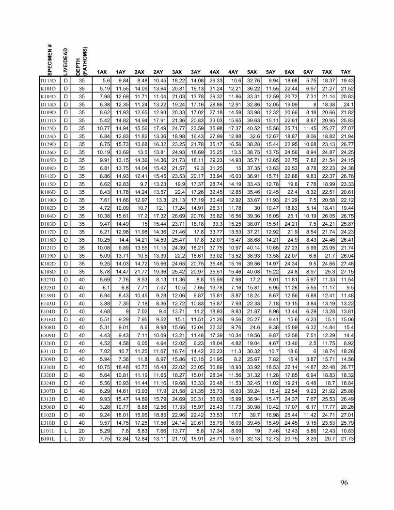
96
SPEC
IMEN
#
LIVE
/DEA
D
DEP
TH
(FA
THO
MS)
1AX 1AY 2AX 2AY 3AX 3AY 4AX 4AY 5AX 5AY 6AX 6AY 7AX 7AYD113D D 35 5.6 9.84 8.48 10.45 18.22 14.08 29.33 10.6 32.76 9.94 18.68 5.75 18.37 19.43K101D D 35 5.19 11.55 14.09 13.64 20.81 16.13 31.24 12.21 36.22 11.55 22.44 6.97 21.27 21.52K103D D 35 7.98 12.69 11.71 11.04 21.03 13.78 29.32 11.86 33.31 12.59 20.72 7.31 21.14 20.83D114D D 35 6.38 12.35 11.24 13.22 19.24 17.16 28.86 12.91 32.86 12.05 19.09 8 18.38 24.1D109D D 35 8.62 11.93 12.65 12.93 20.33 17.02 27.18 14.59 33.98 12.32 20.66 8.18 20.66 21.82D111D D 35 5.42 14.82 14.94 17.91 21.36 20.83 33.03 15.65 39.63 15.11 22.61 8.87 20.95 25.83D125D D 35 10.77 14.94 15.56 17.49 24.77 23.59 35.98 17.37 40.52 15.56 25.71 11.45 25.27 27.07D124D D 35 6.84 12.83 11.82 13.36 18.98 16.43 27.99 12.88 32.6 12.67 18.87 8.06 18.82 21.94D129D D 35 8.75 15.73 10.68 16.32 23.25 21.78 35.17 16.56 38.28 15.44 22.95 10.68 23.13 26.77D126D D 35 10.19 13.69 13.5 13.81 24.93 18.69 35.25 13.5 38.75 13.75 24.56 8.94 24.87 24.25D105D D 35 9.91 13.15 14.36 14.36 21.73 18.11 29.23 14.93 35.71 12.65 22.75 7.82 21.54 24.15D108D D 35 6.81 13.75 14.04 15.42 21.57 19.3 31.25 15 37.35 13.63 22.53 8.78 22.23 24.38D312D D 35 8.86 14.93 12.41 15.45 23.53 20.17 33.94 16.03 36.91 15.71 22.88 9.83 22.37 26.76D115D D 35 6.62 12.83 9.7 13.23 19.9 17.37 28.74 14.19 33.43 12.78 19.8 7.78 18.99 23.33K106D D 35 8.43 11.78 14.24 13.57 22.4 17.26 32.45 12.85 35.46 12.45 22.4 8.32 22.51 20.61D110D D 35 7.61 11.66 12.97 13.3 21.13 17.19 30.49 12.92 33.67 11.93 21.29 7.5 20.58 22.12D102D D 35 4.72 10.09 10.7 12.1 17.24 14.91 26.31 11.78 30 10.47 18.83 5.14 18.41 19.44D104D D 35 10.38 15.61 17.2 17.32 26.69 20.76 36.82 16.56 39.36 16.05 25.1 10.19 26.05 26.75D103D D 35 9.47 14.49 15 15.44 23.71 18.18 33.3 15.25 38.07 15.51 24.21 7.5 24.21 25.87D117D D 35 6.21 12.98 11.98 14.36 21.46 17.8 33.77 13.53 37.21 12.92 21.9 8.54 21.74 24.23D118D D 35 10.25 14.4 14.21 14.59 25.47 17.8 32.07 15.47 38.68 14.21 24.9 8.43 24.46 26.41D121D D 35 10.08 9.89 13.55 11.15 24.39 18.21 37.75 10.97 40.14 10.65 27.23 5.99 23.95 21.74D119D D 35 5.09 13.71 10.5 13.39 22.2 18.61 33.02 13.52 38.93 13.58 22.07 6.6 21.7 26.04K102D D 35 9.25 14.03 14.72 15.66 24.65 20.75 36.48 15.16 39.56 14.97 24.34 9.5 24.65 27.48K108D D 35 8.78 14.47 21.77 19.36 25.42 20.97 35.51 15.46 40.08 15.22 24.8 8.97 25.3 27.15E327D D 40 5.69 7.76 8.53 8.13 11.36 8.8 15.59 7.98 17.2 8.01 11.81 5.97 11.33 11.54E325D D 40 6.1 6.8 7.71 7.07 10.5 7.65 13.78 7.16 15.81 6.95 11.26 5.55 11.17 9.5E139D D 40 6.94 8.43 10.45 9.28 12.06 9.87 15.81 8.87 18.24 8.67 12.56 6.88 12.41 11.48E143D D 40 3.88 7.35 7.18 8.36 12.72 10.83 19.87 7.93 22.33 7.18 13.15 3.84 13.19 13.22E104D D 40 4.68 9 7.02 9.4 13.71 11.2 18.93 9.83 21.87 8.96 13.44 6.29 13.28 13.81E316D D 40 5.51 9.29 7.95 9.52 15.1 11.51 21.26 9.56 25.27 9.41 15.6 6.23 15.1 15.06E508D D 40 5.31 9.01 8.6 9.98 15.66 12.04 22.32 9.76 24.6 9.38 15.89 6.32 14.84 15.4E509D D 40 4.43 9.43 7.11 10.09 13.21 11.48 17.39 10.34 19.56 9.87 12.58 7.51 12.29 14.4E326D D 40 4.52 4.58 6.05 4.64 12.02 6.23 18.04 4.82 19.04 4.67 13.46 2.5 11.75 8.92E311D D 40 7.02 10.7 11.25 11.07 18.74 14.42 26.23 11.3 30.32 10.7 18.6 6 18.74 18.28E309D D 40 5.94 7.36 11.8 8.97 15.86 10.15 21.95 8.2 25.67 7.82 15.4 3.87 15.71 14.56E330D D 40 10.75 18.48 10.75 18.48 22.02 23.05 30.89 18.93 33.92 18.53 22.14 14.87 22.48 26.77E320D D 40 5.64 10.81 11.19 11.65 18.27 15.01 28.34 11.56 31.32 11.28 17.85 6.94 18.83 18.32E324D D 40 5.56 10.93 11.44 11.16 19.68 13.33 26.48 11.53 32.45 11.02 19.21 6.48 18.7 18.84E307D D 40 6.29 14.61 13.93 17.9 21.58 21.35 35.73 16.03 39.24 15.4 22.54 9.23 21.92 25.88E312D D 40 9.93 15.47 14.89 15.79 24.69 20.31 36.03 15.99 38.94 15.47 24.37 7.67 25.53 26.49E506D D 40 3.28 10.77 8.88 12.56 17.33 15.97 25.43 11.73 30.98 10.42 17.07 6.17 17.77 20.26E102D D 40 9.24 18.01 15.95 18.85 22.96 22.42 33.53 17.7 39.7 16.98 25.44 11.42 24.71 27.01E310D D 40 9.57 14.75 17.25 17.56 24.14 20.61 35.79 16.03 39.45 15.49 24.45 9.15 23.53 25.79L101L L 20 5.29 7.6 8.83 7.66 13.77 8.8 17.34 8.09 19 7.46 12.43 5.86 12.43 10.83B101L L 20 7.75 12.84 12.84 13.11 21.19 16.91 26.71 15.01 32.13 12.73 20.75 8.29 20.7 21.73
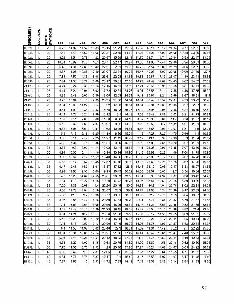
97
SPEC
IMEN
#
LIVE
/DEA
D
DEP
TH
(FA
THO
MS)
1AX 1AY 2AX 2AY 3AX 3AY 4AX 4AY 5AX 5AY 6AX 6AY 7AX 7AYB107L L 20 6.78 14.87 11.57 15.83 23.15 21.29 35.62 15.89 40.11 15.17 24.34 9.77 22.55 26.56B103L L 20 7.58 15.48 16.62 18.66 23.31 22.55 34.58 17.26 38.91 15.99 24.65 10.38 23.06 26.56B102L L 20 8.29 11.54 10.79 11.22 20.87 15.88 32.41 11.76 34.74 11.71 22.44 6.83 22.17 21.03B106L L 20 10.34 16.92 15.3 18.1 25.71 22.17 33.77 19.88 44.85 17.44 27.86 8.94 26.01 30.66B109L L 20 6.46 14.31 12.86 16.42 22.51 20.1 31.93 16.78 37.54 15.09 21.79 9.66 22.39 26.38B108L L 20 4.87 14.96 10.88 17.49 23.07 23.31 30.28 19.47 40.08 15.02 22.65 10.09 21.75 27.7B104L L 20 7.81 17.52 14.85 18.98 23.61 22.98 31.68 19.81 39.87 17.33 25.07 11.49 23.11 28.63B105L L 20 7.34 14.36 13.79 16.08 23.17 20.81 32.68 16.79 41.49 14.62 24.45 8.62 24.32 27.89Z109L L 25 4.24 10.24 9.36 11.16 17.15 14.61 23.19 12.21 29.66 10.98 16.58 6.87 17.11 19.03Z101L L 25 6.44 8.24 10.94 8.92 17.72 12.31 24.76 9.01 27.55 8.11 17.55 4.46 17.55 15.32Z106L L 25 4.35 9.43 10.02 9.89 16.05 12.93 24.31 9.43 30.61 8.21 17.69 3.67 16.51 18.1Z107L L 25 9.27 15.64 16.13 17.33 23.35 21.66 34.54 16.01 37.49 15.52 24.01 9.39 23.29 26.48Z108L L 25 8.81 12.65 14.27 14 22 17.03 30.54 13.84 35.84 12.38 23.03 6.27 22.7 23.35Z105L L 25 5.51 11.92 10.34 12.82 16.75 16.43 26.23 12.19 28.98 12.05 17.38 5.24 16.79 22.62C101L L 30 6.44 7.72 10.21 8.59 12.12 9.1 14.13 8.59 16.43 7.86 12.03 6.21 11.73 10.91D116L L 35 7.37 8.14 9.83 8.66 11.58 9.06 14.13 8.39 15.36 8.08 11.4 6.76 11.37 10.17D110L L 35 6.13 6.67 7.68 7.34 10.97 8.32 14.96 7.28 16.58 6.7 11.31 4.91 11.31 10.06D115L L 35 6.35 8.97 8.61 9.51 11.62 10.26 14.51 9.57 16.83 9.03 12.07 7.37 11.5 12.01D107L L 35 5.4 7.19 8.19 8.25 11.19 8.96 15.04 8 17.27 7.26 11.75 5.46 11.1 10.88D108L L 35 3.88 8.14 7.17 9.25 11.27 11.12 16.77 9.19 19.1 8.32 12.39 6.3 11.34 12.52D109L L 35 5.82 7.31 8.41 8.35 11.24 9.39 15.86 7.93 17.86 7.51 12.29 5.67 11.21 11.18D113L L 35 3.88 9.3 8.02 11.14 13.92 13.41 18.53 11.1 23.26 9.96 13.85 7.07 13.66 16.04D111L L 35 4.94 10.08 8.11 11.16 13.98 13.94 19.96 11.43 23.82 10.27 14.09 7.64 14.79 15.98D102L L 35 3.08 10.69 7.17 11.52 13.48 14.06 20.25 11.63 23.08 10.72 14.17 6.67 14.78 16.92D446L L 35 6.68 12.14 9.57 13.45 17.52 17.16 26.19 13.18 28.49 12.28 18.78 8.62 17.25 19.55D114L L 35 6.47 12.45 14.3 15.61 18.87 17.52 26.3 15.46 33.12 12.05 19.47 8.83 18.97 21.53D103L L 35 6.92 12.83 12.98 15.66 19.19 18.43 26.62 14.85 32.07 13.03 19.7 8.54 18.84 22.37D449L L 35 4.9 13.23 14.87 17.55 20.61 20.03 33.58 15.34 36 14.92 19.87 8.38 19.45 24.25D105L L 35 7.34 11.9 13.22 14.18 19.29 17.42 26.78 13.97 33.47 12.61 20.15 6.89 19.39 22.03D442L L 35 7.29 14.35 10.96 14.4 22.26 20.45 30.9 16.55 36.6 14.01 22.76 8.02 22.31 24.91D445L L 35 9.06 13.79 12.94 15.19 22.57 20.2 29.1 16.77 34.55 14.24 21.89 9.17 22.62 24.26D112L L 35 5.66 12.6 9.2 13.98 18.77 18.05 28.33 13.98 32.7 12.75 19.9 8.64 18.97 20.92D447L L 35 8.05 12.58 13.42 14.16 20.89 17.84 29.79 14.1 34.1 12.84 21.32 8.79 21.37 21.63D443L L 35 7.41 13.65 12.64 15.05 20.56 18.26 28.54 15.17 34.21 13.65 20.56 9.32 21.35 22.64D452L L 35 8.48 13.42 15.11 16.29 21.23 19.15 29.03 15.89 36.56 14.15 24.88 8.82 21.4 23.36D440L L 35 6.01 14.21 10.9 15.17 20.56 21.68 32.8 15.67 36.12 14.55 24.15 8.09 21.35 25.39D106L L 35 6.46 10.23 8.96 10.79 18.63 15.88 29.57 10.43 32.27 9.77 20.41 5.5 19.14 19.29D104L L 35 7.11 12.13 14.52 15.13 20.56 17.46 26.29 15.08 34.77 11.93 21.27 7.82 20.81 21.37D441L L 35 6.4 14.55 11.97 15.62 23.48 22.3 36.01 15.62 41.01 14.49 23.2 9.1 22.92 25.28D450L L 35 10.04 16.31 16.05 17.14 28.21 21.36 37.42 16.44 40.49 15.61 23.47 7.48 25.65 26.86D448L L 35 6.04 13.44 13.28 15.54 20.42 18.32 27.34 15.8 33.75 13.59 20.21 8.19 19.73 22.31D101L L 35 6.31 14.22 11.07 16.15 19.68 20.75 31.82 14.92 33.69 14.55 20.16 9.52 19.89 25.08D517L L 35 7.73 14.35 15.78 17.92 25 23.18 35.78 17.27 43.24 14.67 24.67 8.05 24.22 28.89E144L L 40 6.08 6.49 9.3 7.87 12.05 8.6 15.32 7.37 17.22 6.64 11.55 4.71 11.52 9.68E141L L 40 6.81 7.77 8.75 8.37 12.17 9.1 15.42 8.17 16.58 7.97 11.97 6.17 11.45 10.9E143L L 40 7.57 6.65 10 7.33 11.72 7.63 14.18 7.12 16.05 6.85 12.14 5.58 11.63 8.99

98
SPEC
IMEN
#
LIVE
/DEA
D
DEP
TH
(FA
THO
MS)
1AX 1AY 2AX 2AY 3AX 3AY 4AX 4AY 5AX 5AY 6AX 6AY 7AX 7AYE114L L 40 2.72 6.63 6.76 7.92 9.41 8.91 15.05 7 17.3 6.73 10.2 4.33 9.65 10.3E145L L 40 6.88 7.2 8.54 7.69 11.37 8.1 14.08 7.66 16.29 7.2 11.45 5.65 11.42 9.65E146L L 40 6.07 7.63 9.58 8.76 11.38 9.29 15.14 8.39 17.6 7.8 11.95 5.82 11.47 11.27E142L L 40 5.47 5.5 8.56 6.61 11.35 7.37 16.24 5.88 17.32 5.71 11.88 3.7 11.32 9.52E127L L 40 3.74 8.52 9.14 9.92 14.82 12.65 18.99 10.7 25.95 9.3 14.16 5.49 15.14 15.52E117L L 40 4.57 9.24 9.17 9.53 14.77 10.95 19.55 9.6 24.33 9.17 14.84 5.42 13.92 13.84E107L L 40 7.36 8.26 9.91 9.34 13.02 10.45 17.03 8.92 18.41 8.38 13.62 6.35 12.84 11.53E133L L 40 5.26 8.75 8.68 10.11 13.53 13.01 21.4 10.11 24.01 9.67 16.65 6.25 12.94 14.67E119L L 40 3.79 6.85 5.97 7.84 9.74 9.05 14.87 7.69 16.2 6.95 10.72 4.51 9.79 10.74E135L L 40 1.91 8.15 5.69 9.97 10.03 11.3 15.69 9.6 19.51 8.18 10.81 5.35 9.97 13.15E129L L 40 4.35 8.91 8.47 10.78 12.52 12.55 18.74 10.44 21.7 9.86 13.5 6.94 13.37 14.22E118L L 40 2.92 8.02 6.52 9 11.5 10.38 15.42 9.06 20.37 7.65 11.82 4.95 11.25 12.79E131L L 40 3.65 8.87 10.11 10.84 14.74 12.66 19.01 11.2 27.01 9.09 16.13 5.62 14.49 16.71E132L L 40 3.54 9.11 8.63 10.44 15.53 12.36 21.44 10.22 25.46 9.11 13.69 5.65 14.58 15.65E102L L 40 4.62 12.06 6.43 12.94 17.77 16.47 22.52 14.12 28.49 11.6 17.82 8.32 16.76 19.87E136L L 40 6.89 11.55 10.23 12.78 17.12 15.8 26.57 12.47 28.9 11.55 18.26 7.35 18.22 19.86E138L L 40 4.3 8.44 8.59 10.42 13.19 12.2 19.2 9.77 23.83 8.59 15.02 5.28 13.49 14.71E120L L 40 4.41 10 8.11 11.63 15.92 14.37 20.55 12.18 25.37 10.93 15.63 7.22 14.44 17.07E116L L 40 10.55 13.03 15.41 14.67 22.8 16.89 31.29 13.19 34.14 12.45 21.95 7.44 21.16 22.06E128L L 40 6.95 12.75 12.36 14.97 18.88 17.24 26.9 13.57 31.19 12.27 18.88 8.16 19.07 21.83E122L L 40 6.02 15.16 10.16 15.75 19.95 20.97 28.12 16.51 36.02 15 20.59 9.3 20.7 25.81E124L L 40 5.63 11.88 12.77 14.69 18.78 16.38 26.29 13.38 32.39 10.75 18.54 6.43 18.5 20.8E110L L 40 8.01 12.61 12.27 13.92 22.33 17.1 33.07 12.56 35.17 11.76 21.25 5.62 21.08 22.84E108L L 40 6.78 9.39 9.65 10.5 18.74 15.52 27.93 10.85 32.66 9.39 16.38 4.07 18.79 19.59E104L L 40 6.17 13.34 11.85 14.72 20.04 18.29 28.7 14.14 33.27 12.97 20.04 7.02 20.31 23.71E103L L 40 4.7 11.39 8.91 12.82 16.58 16.19 27.47 12.62 30.99 11.93 19.65 5.89 17.47 21.73E123L L 40 8.05 17.52 11.76 17.02 28.85 23.28 38.32 17.27 43.46 16.71 25.63 9.53 26.49 29.78E101L L 40 7.75 14.04 9.55 14.91 24.17 21.2 34.25 16.66 40.02 13.46 24 8.85 25.16 24.64E125L L 40 5.67 14.61 13.17 18.06 22.06 22.5 31.28 17.39 38.56 14.5 21.33 9.44 22.33 27.83E130L L 40 6.05 13.28 12.35 15.22 19.22 18.25 27.22 14.61 32.96 12.97 19.68 8.25 20.09 21.99E109L L 40 5.07 12.08 11 12.48 22.06 18.18 32.94 12.77 38.24 12.03 20.57 6.21 21.77 25.59E112L L 40 8.84 16.09 17.15 18.82 24.93 23.6 35.17 19.68 41.89 17.75 25.27 6.78 26.46 28.26E121L L 40 4.83 10.85 13.28 13.98 19.25 16.07 27.41 12.84 34.08 10.05 20.25 5.17 18.41 20.95E105L L 40 7.09 14.5 15.94 17.32 22.59 20.02 33.45 15.5 40.1 15.5 24.35 7.09 22.72 26.99E111L L 40 2.55 10.41 8.18 11.73 15.41 14.82 24.18 11 28.45 10.45 15.91 5.32 15.64 18.73E106L L 40 5.34 13.87 9.21 14.32 17.69 18.03 27.86 14.21 32.18 13.37 18.2 7.98 18.14 24.15E113L L 40 8.91 12.87 16.57 15.71 25.15 21.32 36.23 15.84 42.37 14.39 25.28 6.01 25.01 25.81E134L L 40 7.69 15.78 13.47 18.38 22.66 22.89 36.88 15.49 38.67 15.61 23.58 8.32 22.72 27.98
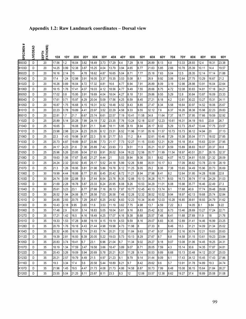
99
Appendix 1.2: Raw Landmark coordinates – Dorsal view
SPEC
IMEN
#
LIVE
/DEA
D
DEPT
H (F
ATHO
MS)
1DX 1DY 2DX 2DY 3DX 3DY 4DX 4DY 5DX 5DY 6DX 6DY 7DX 7DY 8DX 8DY 9DX 9DYB503D D 20 17.56 1.2 16.04 3.82 18.49 3.73 17.29 4.4 7.29 8.18 26.89 8.13 4.8 13.33 28.93 12.4 18.31 23.38B103D D 20 14.25 0.99 12.38 3.87 15.25 4.04 13.79 3.94 4.65 6.77 21.63 5.85 2.66 10.78 25.39 10.11 14.4 19.57B502D D 20 16.16 2.14 15 4.78 18.62 4.87 16.65 5.04 8.71 7.77 25.18 7.63 5.04 12.5 28.35 12.14 17.14 21.88B104D D 20 17.4 1.24 12.98 3.91 16.05 3.37 15.35 3.53 5.08 8.1 26.9 9.92 3.06 12.64 27.75 13.29 16.67 21.2B102D D 20 16.26 0.89 16.04 4.72 17.32 4.81 16.6 4.77 6.94 7.91 26.89 8.09 3.19 12.98 28.98 13.91 16.04 22.64B106D D 20 18.15 1.76 17.41 4.07 19.03 4.12 18.56 4.77 9.49 7.55 28.66 8.75 4.72 12.08 30.83 14.81 17.18 24.21B505D D 20 17.02 0.8 15.95 3.91 19.69 4.04 18.04 4.27 8.18 7.51 29.86 9.55 5.29 12.8 30.84 13.87 16.09 23.33B504D D 20 17.61 0.71 15.97 4.29 20.04 5.09 17.56 4.25 6.59 8.45 27.21 8.18 4.2 12.61 30.22 13.27 15.31 24.11B105D D 20 16.87 1.75 16.68 4.15 19.31 4.52 18.48 4.52 8.43 8.85 27.47 8.34 5.58 16.64 30.97 14.52 18.06 25.67B101D D 20 22.23 0.78 19.89 4.41 23.97 3.52 22.29 4.58 9.33 9.55 32.12 7.6 6.37 16.26 38.38 15.98 22.23 29.83B501D D 20 22.81 1.7 21.7 6.67 23.74 6.61 22.57 7.19 10.41 11.58 34.8 11.64 7.37 18.77 37.95 17.66 19.59 32.92Y102D D 25 20.89 5.14 20.28 7.99 24.19 7.32 23.35 7.76 13.24 12.18 32.57 12.23 10.61 16.31 34.19 19.5 23.8 26.7Z104D D 25 16.65 3 16.08 5.81 21.1 6.48 18.11 5.95 8.19 8.94 26.17 8.02 5.29 12.73 29.47 13.44 17.75 23.57Y101D D 25 23.98 2.98 22.24 6.23 25.05 6.12 23.31 6.52 11.96 11.91 35.16 11.57 10.73 15.73 36.12 14.94 20 27.13Z106D D 25 22.3 1.43 19.98 4.97 22.3 5.18 21.77 5.5 11.2 8.4 32.61 10.46 7.29 15.38 35.04 17.71 18.02 27.85Y103D D 25 20.73 4.87 19.89 8.07 23.86 7.73 21.17 7.73 12.27 11.15 33.83 12.21 8.29 15.18 35.4 15.63 22.91 27.95Z102D D 25 24.17 4.23 21.6 7.36 25.89 7.42 23.93 7.3 9.51 11.9 35.21 10.37 8.59 15.89 38.83 16.07 20.37 30.8Z105D D 25 25.96 5.26 23.85 9.04 27.63 8.91 26.02 9.04 16.22 12.56 35.77 11.99 11.54 18.97 40.51 20.7 26.15 32.37Z108D D 25 19.63 1.06 17.67 5.45 21.27 4.44 21 5.03 8.94 9.36 30.1 8.62 4.07 16.72 34.81 15.55 21.32 28.09Z103D D 25 24.24 2.32 20.92 6.45 25.17 5.52 24.18 5.99 12.26 9.88 35.51 10.17 9.3 17.09 36.62 13.78 23.19 28.19Z107D D 25 21.3 1.26 18.95 5.81 21.98 5.86 19.78 6.12 11.25 9.05 29.2 8.06 7.38 15.65 34.49 15.96 20.73 26.69C106D D 30 19.99 4.44 18.88 6.77 21.85 6.45 20.42 6.72 11.21 8.94 27.98 8.41 8.2 12.64 31.95 14.28 18.88 22.8C103D D 30 24.74 3.59 22.88 5.9 27.44 6.54 23.78 6.35 12.88 10.13 36.28 10.71 8.53 16.73 39.74 17.18 24.29 31.03C105D D 30 21.69 2.28 18.78 5.87 23.33 6.24 20.95 6.08 9.26 10.53 34.29 11.01 6.08 15.98 35.77 16.46 22.49 27.3C104D D 30 25.61 3.23 23.1 6.77 27.68 7.16 26.13 7.87 10.77 12.45 40.13 13.74 9.1 17.68 40.9 17.74 29.48 29.68C102D D 30 26.52 1.94 24.06 6.77 28.58 7.03 26.58 7.48 12.26 12.32 38.52 10.52 9.94 18.97 42.13 19.68 25.74 32.84C101D D 30 24.85 2.93 20.75 7.29 26.67 6.25 24.92 6.83 12.23 10.34 36.49 12.03 10.28 16.85 39.81 18.93 24.79 31.62D130D D 35 10.43 2.18 9.95 3.65 11.6 3.53 11.19 3.62 7.75 4.98 13.7 4.59 7.22 6.3 14.05 6.1 9.84 9.22D106D D 35 17.48 2.9 16.91 5.14 18.83 5.05 18.04 5.61 9.16 8.83 25.42 8.32 6.73 13.46 28.69 13.27 17.24 22.71D127D D 35 17.21 1.42 16.5 4.16 18.49 4.25 17.07 4.16 9.38 6.68 25.57 7.48 6.41 11.68 27.69 11.9 18 21.76D101D D 35 19.33 1.53 17.28 4.68 19.19 4.15 19.19 4.53 9.59 8.16 29.07 8.83 6.35 12.89 31.41 14.46 16.99 23.25D128D D 35 20.79 1.76 19.18 4.43 21.44 4.98 19.98 4.73 11.98 8 27.33 8 8.46 15.3 31.21 14.09 21.34 25.02K104D D 35 20.32 4.95 18.16 7.74 21.63 7.74 20.21 7.32 11.84 9.63 27.47 9.37 9.37 12.16 30.74 12.21 19.63 20.63D112D D 35 19.39 2.81 16.93 6.39 20.05 5.22 19.03 5.73 10.13 8.29 27.67 8.7 6.8 14.58 31.15 13.61 19.23 23.84K105D D 35 20.83 3.74 19.41 6.7 23.1 6.96 21.04 6.7 11.34 9.02 29.27 9.18 9.07 13.08 31.06 14.45 18.25 24.31D107D D 35 18.19 1.34 17.59 3.47 19.58 3.66 18.47 3.89 9.07 6.71 28.05 7.59 4.3 15.14 30.6 14.35 17.87 24.81D122D D 35 20.43 3.26 19.09 5.94 20.69 5.78 20.21 6.31 11.28 9.14 30.53 9.89 6.68 15.13 33.48 14.12 20.37 25.03D123D D 35 20.21 2.57 19.79 4.49 21.5 4.97 21.23 6.1 9.79 9.14 31.44 9.09 6.1 17.43 34.12 15.45 17.43 27.86D116D D 35 19.3 3.34 17.4 5.6 20.58 5.44 18.89 6.21 9.7 8.42 29.62 9.6 5.7 13.91 31.78 14.89 19.3 24.74K107D D 35 21.96 1.45 19.5 4.47 21.73 4.08 21.73 4.86 14.58 6.87 30.73 7.99 6.48 15.08 36.15 15.64 21.84 28.27D120D D 35 23.55 5.04 21.25 8.11 23.87 8.11 23.3 8.3 12 12.06 33.57 12.38 8.62 19.27 37.4 18.89 25.08 31.08
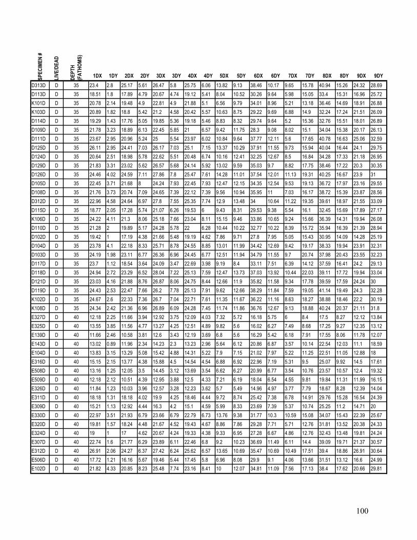
100
SPEC
IMEN
#
LIVE
/DEA
D
DEPT
H (F
ATHO
MS)
1DX 1DY 2DX 2DY 3DX 3DY 4DX 4DY 5DX 5DY 6DX 6DY 7DX 7DY 8DX 8DY 9DX 9DYD313D D 35 23.4 2.8 25.17 5.61 26.47 5.8 25.75 6.06 13.82 9.13 38.46 10.17 9.65 15.78 40.94 15.26 24.32 28.69D113D D 35 18.51 1.8 17.89 4.79 20.67 4.74 19.12 5.41 8.04 10.52 30.26 9.64 5.98 15.05 33.4 15.31 16.96 25.72K101D D 35 20.78 2.14 19.48 4.9 22.81 4.9 21.88 5.1 6.56 9.79 34.01 8.96 5.21 13.18 36.46 14.69 18.91 26.88K103D D 35 20.89 1.82 18.8 5.42 21.2 4.58 20.42 5.57 10.63 8.75 29.22 9.69 6.88 14.9 32.24 17.24 21.51 26.09D114D D 35 19.29 1.43 17.76 5.05 19.85 5.36 19.18 5.46 8.83 8.32 29.74 9.64 5.2 15.36 32.76 15.51 18.01 26.89D109D D 35 21.78 3.23 18.89 6.13 22.45 5.85 21 6.57 9.42 11.75 28.3 9.08 8.02 15.1 34.04 15.38 20.17 26.13D111D D 35 23.67 2.95 20.96 5.24 25 5.54 23.97 6.02 10.84 9.64 37.77 12.11 5.6 17.65 40.78 16.63 25.06 32.59D125D D 35 26.11 2.95 24.41 7.03 26.17 7.03 25.1 7.15 13.37 10.29 37.91 11.55 9.73 15.94 40.04 16.44 24.1 29.75D124D D 35 20.64 2.51 18.98 5.78 22.62 5.51 20.48 6.74 10.16 12.41 32.25 12.67 8.5 16.84 34.28 17.33 21.18 26.95D129D D 35 21.83 3.31 23.02 5.62 26.57 5.68 24.14 5.92 13.02 9.59 35.03 9.7 8.82 17.75 38.46 17.22 20.3 30.35D126D D 35 24.46 4.02 24.59 7.11 27.86 7.8 25.47 7.61 14.28 11.01 37.54 12.01 11.13 19.31 40.25 16.67 23.9 31D105D D 35 22.45 3.71 21.68 8 24.24 7.93 22.45 7.93 12.47 12.15 34.35 12.54 9.53 19.13 36.72 17.97 23.16 29.55D108D D 35 21.76 3.73 20.74 7.09 24.65 7.39 22.12 7.39 9.56 10.94 35.95 11 7.03 16.17 38.72 15.39 23.87 28.56D312D D 35 22.96 4.58 24.64 6.97 27.8 7.55 25.35 7.74 12.9 13.48 34 10.64 11.22 19.35 39.61 18.97 21.55 33.09D115D D 35 18.77 2.05 17.28 5.74 21.07 6.26 19.53 6 9.43 8.31 29.53 9.38 5.54 16.1 32.45 15.69 17.89 27.17K106D D 35 24.22 4.11 21.3 8.06 25.18 7.66 23.04 8.11 15.15 9.46 33.86 10.65 9.24 15.66 36.39 14.31 19.94 26.08D110D D 35 21.28 2 19.89 5.17 24.28 5.78 22 6.28 10.44 10.22 32.77 10.22 8.39 15.72 35.94 16.39 21.39 28.94D102D D 35 19.42 1 17.19 4.38 21.66 5.48 19.19 4.62 7.86 9.71 27.8 7.95 5.05 15.43 30.95 14.09 14.28 25.19D104D D 35 23.78 4.1 22.18 8.33 25.71 8.78 24.55 8.85 13.01 11.99 34.42 12.69 9.42 19.17 38.33 19.94 23.91 32.31D103D D 35 24.19 1.98 23.11 6.77 26.36 6.96 24.45 6.77 12.51 11.94 34.79 11.55 9.7 20.74 37.98 20.43 23.55 32.23D117D D 35 23.7 1.12 18.54 3.64 24.09 3.47 22.69 3.98 9.19 8.4 33.11 7.51 6.39 14.12 37.59 16.41 24.2 29.13D118D D 35 24.94 2.72 23.29 6.52 28.04 7.22 25.13 7.59 12.47 13.73 37.03 13.92 10.44 22.03 39.11 17.72 19.94 33.04D121D D 35 23.03 4.16 21.88 8.76 26.87 8.06 24.75 8.44 12.66 11.9 35.82 11.58 9.34 17.78 39.59 17.59 24.24 30D119D D 35 24.43 2.53 22.47 7.66 26.2 7.78 25.13 7.91 9.62 12.66 38.29 11.84 7.59 19.05 41.14 19.49 24.3 32.28K102D D 35 24.67 2.6 22.33 7.36 26.7 7.04 22.71 7.61 11.35 11.67 36.22 11.16 8.63 18.27 38.88 18.46 22.2 30.19K108D D 35 24.34 2.42 21.36 6.96 26.89 6.09 24.28 7.45 11.74 11.86 36.76 12.67 9.13 18.88 40.24 20.37 21.11 31.8E327D D 40 12.18 2.25 11.66 3.94 12.92 3.75 12.09 4.03 7.32 5.72 16.18 5.75 6 8.4 17.5 8.27 12.12 13.84E325D D 40 13.55 3.85 11.56 4.77 13.27 4.25 12.51 4.89 9.82 5.6 16.02 6.27 7.49 8.68 17.25 9.27 12.35 13.12E139D D 40 11.66 2.46 10.58 3.81 12.6 3.43 12.19 3.69 6.8 5.6 16.29 5.42 6.18 7.91 17.55 8.06 11.78 12.07E143D D 40 13.02 0.89 11.96 2.34 14.23 2.3 13.23 2.96 5.64 6.12 20.86 6.87 3.57 10.14 22.54 12.03 11.1 18.59E104D D 40 13.83 3.15 13.29 5.08 15.42 4.88 14.31 5.22 7.9 7.15 21.02 7.97 5.22 11.25 22.51 11.05 12.88 18E316D D 40 15.15 2.15 13.77 4.38 15.88 4.5 14.54 4.54 6.88 6.92 22.96 7.19 5.31 9.5 25.07 9.92 14.5 17.61E508D D 40 13.16 1.25 12.05 3.5 14.45 3.12 13.69 3.54 6.62 6.27 20.99 6.77 3.54 10.76 23.57 10.57 12.4 19.32E509D D 40 12.18 2.12 10.51 4.39 12.95 3.88 12.5 4.33 7.21 6.19 18.04 6.54 4.55 9.81 19.84 11.31 11.99 16.15E326D D 40 11.84 1.23 10.03 3.96 12.57 3.28 12.23 3.62 5.7 5.49 14.96 4.97 3.77 7.79 18.67 8.28 12.39 14.04E311D D 40 18.18 1.31 18.18 4.02 19.9 4.25 18.46 4.44 9.72 8.74 25.42 7.38 6.78 14.91 29.76 15.28 16.54 24.39E309D D 40 15.21 1.13 12.92 4.44 16.3 4.2 15.1 4.59 5.99 8.33 23.69 7.39 5.37 10.74 25.25 11.2 14.71 20E330D D 40 22.97 3.51 21.93 6.79 23.66 6.79 22.79 6.73 13.76 9.38 31.77 10.3 10.59 15.08 34.07 15.43 22.39 25.67E320D D 40 19.81 1.57 18.24 4.48 21.67 4.52 19.43 4.67 8.86 7.86 29.28 7.71 5.71 12.76 31.81 13.52 20.38 24.33E324D D 40 19 1 17 4.62 20.67 4.24 19.33 4.38 9.33 6.95 27.28 6.67 4.86 12.76 32.43 13.48 19.81 24.24E307D D 40 22.74 1.6 21.77 6.29 23.89 6.11 22.46 6.8 9.2 10.23 36.69 11.49 6.11 14.4 39.09 19.71 21.37 30.57E312D D 40 26.91 2.06 24.27 6.37 27.42 6.24 25.62 6.57 13.65 10.69 35.47 10.69 10.49 17.51 39.4 18.86 26.91 30.64E506D D 40 17.72 1.21 16.16 5.67 19.46 5.44 17.45 5.8 6.96 8.08 29.9 9.1 4.06 13.66 31.51 13.12 16.6 24.99E102D D 40 21.82 4.33 20.85 8.23 25.48 7.74 23.16 8.41 10 12.07 34.81 11.09 7.56 17.13 38.4 17.62 20.66 29.81
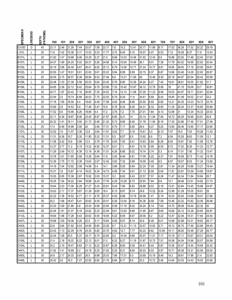
101
SPEC
IMEN
#
LIVE
/DEA
D
DEPT
H (F
ATHO
MS)
1DX 1DY 2DX 2DY 3DX 3DY 4DX 4DY 5DX 5DY 6DX 6DY 7DX 7DY 8DX 8DY 9DX 9DYE310D D 40 23.11 2.46 21.26 7.44 25.07 7.56 23.17 7.8 10.2 12.41 35.77 11.86 8.11 17.02 38.29 17.02 20.22 29.19L101L L 20 11.6 1.42 10.38 3.17 12.53 3.23 11.77 3.72 6.45 5.15 16.57 5.47 4.53 7.12 18.28 8.37 11.8 13.43B101L L 20 21.82 1.47 19.98 6.46 23.29 5.37 21.5 6.68 13.03 10.48 31.92 12.43 8.9 16.88 33.55 17.48 23.45 27.63B107L L 20 24.37 1.69 24.25 5.02 26.37 5.26 24.98 5.14 10.64 10.46 36.1 9.01 7.38 17.78 40.52 16.99 22.62 30.54B103L L 20 25.19 2.88 24.49 6.67 26.41 6.92 25.13 6.79 13.08 10.77 37.24 10.77 8.91 18.85 39.93 17.18 25.06 29.61B102L L 20 20.93 1.47 19.51 5.61 22.62 5.61 20.22 5.94 8.99 9.59 32.15 9.37 6.87 13.68 33.46 14.28 22.83 26.87B106L L 20 26.05 2.15 26.57 6.38 28.94 6.53 27.46 6.9 13.21 11.95 40 10.46 9.35 20.19 44.97 20.04 26.42 35.99B109L L 20 22.48 1.33 21.39 5.58 25.03 5.64 23.45 5.76 8.85 10.36 34.24 9.27 7.45 16.61 38.61 16.55 21.82 31.7B108L L 20 24.85 2.36 22.12 6.42 25.64 6.79 23.88 7.33 10.42 10.97 38.12 12.79 5.58 18 41.15 18.06 23.7 30.91B104L L 20 24.71 1.87 23.42 7.16 26.65 7.35 24.52 7.16 12.13 11.68 37.29 11.23 8.58 19.03 40.97 18.71 23.61 32.84B105L L 20 22.94 2.5 19.74 6.99 26.53 7.75 22.05 6.79 9.29 11.6 34.61 9.68 6.54 18.84 41.08 16.02 21.47 33.2Z109L L 25 17.18 1.85 16.56 4.4 18.63 4.49 17.58 4.93 8.06 8.99 25.55 8.55 4.85 13.21 30.35 14.23 19.73 23.79Z101L L 25 15.69 2.8 14.53 5.9 17.46 5.47 15.9 5.78 6.34 8.28 24.31 8.32 4.65 11.25 26.34 12.37 16.85 20.69Z106L L 25 17.52 0.6 15.96 4.26 18.89 4.4 17.2 3.76 7.2 7.75 27.01 7.84 4.13 12.98 31 13.34 16.33 24.53Z107L L 25 22.11 4.36 19.87 8.06 23.45 8.97 21.57 8.85 9.21 14 33.14 11.94 7.94 18.72 36.29 16.96 23.81 30.6Z108L L 25 20.32 1.41 18.11 5.95 21.73 5.46 21.35 5.73 9.89 8.49 31.78 11.95 6.16 17.35 32.86 17.46 17.51 27.08Z105L L 25 17.4 0.46 14.98 3.56 20 3.56 17.31 4.75 7.17 8.95 28.4 9.27 5.25 13.65 29.36 13.65 17.17 24.84C101L L 30 12.52 1.8 11.57 3.38 12.8 3.64 11.91 3.52 7.7 5.16 15.61 5.3 6.13 7.47 16.5 7.53 10.28 11.43D116L L 35 11.31 4.38 10.7 5.35 11.85 5.32 11.31 5.5 8.57 6.5 13.92 6.6 7.2 8.54 15.26 8.63 11.09 12.1D110L L 35 11.58 2.42 10.8 3.96 12.4 3.78 11.76 4.05 7.92 5.41 15.63 5.84 6.26 8.04 16.81 7.92 11.58 12.76D115L L 35 12.37 3.77 11.2 5.19 13.22 4.92 12.37 5.01 7.3 6.91 15.78 5.95 6.55 8.72 17.02 8.39 11.23 12.77D107L L 35 11.29 2.49 10.72 4.38 12.18 4.38 11.51 4.26 6.66 6.02 15.74 5.74 5.3 8.14 17.51 7.95 11.32 13.47D108L L 35 12.78 1.61 11.65 3.58 13.29 3.64 11.9 3.45 6.46 4.81 17.09 5.22 4.37 7.91 19.59 8.73 11.42 14.78D109L L 35 12.39 1.75 11.72 3.38 13.63 3.57 12.42 3.92 7.32 5.99 16.59 5.45 6.5 8.57 18.57 8.53 11.34 13.92D113L L 35 14.18 1.04 13.92 3.58 14.96 3.4 14.1 3.69 5.93 6.64 22.24 7.05 3.81 11.34 24.29 10.86 13.21 19.44D111L L 35 15.31 1.8 13.67 4.14 16.02 4.34 14.73 4.06 7.34 6.91 21.13 6.95 5.04 11.91 23.91 10.59 14.69 18.67D102L L 35 15.55 0.85 13.38 2.87 15.92 3.05 15.37 3.2 6.62 6.43 22.57 7.57 4.26 11.47 24.34 11.84 16.84 20.7D446L L 35 18.25 1.54 16.22 3.84 18.88 4.43 17.76 4.29 10.26 6.73 25.93 7.64 6.6 13.1 28.46 12.51 14.82 21.73D114L L 35 19.64 2.03 17.06 6.29 21.27 5.43 20.81 5.43 7.66 8.83 28.88 8.53 5.18 13.91 32.64 13.45 18.88 24.97D103L L 35 19.02 2.11 17.37 5.67 21.39 6.65 18.4 6.13 8.97 9.74 29.9 10.52 6.34 12.99 31.29 15.05 18.61 25D449L L 35 22.22 1.38 19.52 4.71 21.11 4.76 20.37 4.55 6.88 10.79 29.58 7.41 5.19 16.03 35.93 14.66 19.47 27.88D105L L 35 20.2 1.68 18.47 5.41 20.82 4.54 20.51 5.26 12.04 8.16 30.36 9.59 7.09 15.46 33.32 15.82 23.06 26.48D442L L 35 23.33 1.69 21.86 4.8 25.03 4.69 23.95 5.08 11.19 8.02 34.24 8.14 7.63 14.75 38.08 16.44 22.32 30D445L L 35 22.94 1.81 21.07 5.16 23.62 5.33 22.09 5.61 12.63 8.89 31.95 8.67 9.69 16.66 35.12 14.28 20.85 26.97D112L L 35 18.64 1.88 17.28 5.43 20.62 4.54 18.95 5.22 8.09 8.67 28.56 8.2 5.22 13.47 32.06 15.51 17.65 24.54D447L L 35 19.68 1.65 19.36 4.26 22.5 5.11 19.84 4.95 9.57 8.14 30.9 8.46 6.01 14.68 32.98 14.31 18.62 26.17D443L L 35 23.8 2.84 21.92 6.53 24.65 6.65 23.29 6.7 12.21 11.13 33.57 10.62 9.71 18.12 36.75 17.49 22.66 28.45D452L L 35 23.42 1.13 22.29 4.76 25.35 4.82 23.76 4.82 12.7 7.77 35.22 8.62 10.09 16.11 38.05 15.48 27.28 26.77D440L L 35 22.54 1.58 20.5 5.37 24.17 4.74 22.65 5.2 10.34 9.66 35.07 11.01 7.17 15.19 37.11 15.87 24.51 29.54D106L L 35 21.4 2.18 19.22 6.22 22.12 6.01 21.5 6.32 9.27 11.19 31.87 10.73 7.51 16.58 34.04 15.96 20.57 26.58D104L L 35 20.2 2.19 18.47 6.63 21.12 6.22 20.87 6.28 8.83 9.39 30.41 9.44 5.87 15.36 33.47 14.54 19.69 26.43D441L L 35 21.92 1.41 19.89 5.2 24.18 5.25 21.92 5.25 9.21 8.64 35.03 8.53 4.97 15.71 39.38 15.31 20.56 29.04D450L L 35 24.9 2.17 24.33 5.67 26.5 6.88 25.03 7.96 17.01 9.3 33.69 10.19 9.49 19.3 39.81 17.96 21.4 32.93D448L L 35 20.42 2.6 18.3 7.27 22.92 6.84 21.75 6.84 8.17 9.6 32.2 10.72 5.46 14.64 33.53 14.43 19.05 25.99

102
SPEC
IMEN
#
LIVE
/DEA
D
DEPT
H (F
ATHO
MS)
1DX 1DY 2DX 2DY 3DX 3DY 4DX 4DY 5DX 5DY 6DX 6DY 7DX 7DY 8DX 8DY 9DX 9DYD101L L 35 22.6 1.69 20.45 6.55 25.2 6.55 23.84 7.12 11.41 11.58 34.01 12.2 7.68 17.91 36.72 17.97 21.81 30.51D517L L 35 25.81 2.48 23.46 8.63 27.51 8.63 25.61 8.76 11.63 11.5 40.84 13.46 8.1 18.43 43.78 20.52 29.14 32.61E144L L 40 10.75 2.37 9.67 3.66 11.25 3.6 10.61 3.46 6.39 5.07 14.74 5.42 4.86 7.79 15.94 7.76 10.37 12.25E141L L 40 11.93 2.33 10.99 3.92 12.55 3.86 12.14 4.01 7.66 5.92 16.03 5.51 6.57 7.99 16.59 7.1 10.9 11.85E143L L 40 12.02 1.97 11.04 3.68 12.55 3.56 12.13 3.65 8.54 4.62 15.11 4.68 7.51 6.48 15.96 6.33 11.49 10.31E114L L 40 9.1 0.87 8.97 2.15 10.69 2.31 9.85 2.36 4.82 4 14.05 3.67 2.64 8.05 17.26 7.15 11.15 13.08E145L L 40 11.8 1.92 10.69 3.29 12.76 3.15 11.48 3.2 8.04 4.75 15.17 4.81 6.76 6.35 16.25 6.67 11.85 10.14E146L L 40 11.71 0.71 10.44 2.59 11.97 2.59 11.76 2.59 6.91 4.38 15.44 4.32 5.65 6.29 17.41 7.38 12.26 12.03E142L L 40 11.21 0.79 10.72 2.68 12.44 2.71 11.97 2.88 6.38 4.54 15.87 4.66 4.95 6.73 17.33 7.92 10.78 12.26E127L L 40 16.1 1.69 14.61 3.86 16.3 3.9 15.71 3.9 7.76 6.1 23.97 6.53 3.58 10.2 26.57 10.87 14.29 19.21E117L L 40 13.75 2.13 12.81 4.62 13.86 4.66 13.39 4.69 5.45 6.82 23.07 8.19 3.93 9.6 24.98 10.87 14.91 18.74E107L L 40 11.75 1.72 10.81 3.89 12.86 3.77 11.87 3.86 7.14 5.6 15.75 5.33 6.05 7.08 17.2 7.74 11.2 12.41E133L L 40 14.53 2.25 13.67 4.27 15.99 4.04 15.43 3.89 7.27 6.67 21.27 6.55 4.46 10.56 24.75 10.26 15.73 18.57E119L L 40 10.42 1.11 9.44 2.65 11.67 3.49 10.4 3.07 5.13 4.89 14.47 4.84 3.44 7.91 15.95 7.28 9.13 12.75E135L L 40 10.21 1.32 9.97 3.38 11.62 3.76 11.24 3.68 4.06 6.41 17.94 5.94 2.62 9.15 20.32 8.74 12.47 15.32E129L L 40 14.37 2.45 13.18 4.44 15.28 4.55 13.57 4.69 7.45 6.64 20.87 7.41 4.48 9.3 22.27 10.38 14.97 16.96E118L L 40 12.19 0.45 11.17 2.83 13.34 2.99 12.29 2.99 6.3 4.93 18.62 5.7 2.83 9.07 21.07 9.01 11.87 15.82E131L L 40 16.19 1.23 13.58 3.47 15.52 3.51 14.48 3.21 5.04 6.72 23.69 7.31 2.87 11.38 26.49 12.13 17.39 20.52E132L L 40 14.74 0.34 12.99 3.1 15.52 3.21 14.22 3.36 5.34 6.57 21.75 5.9 3.17 10.45 25.04 11.98 14.25 21.19E102L L 40 16.79 1.65 15.32 4.81 18.23 4.39 16.54 4.98 6.84 8.14 27.05 8.1 4.73 12.53 29.11 11.69 14.26 23.12E136L L 40 14.65 3.64 15.62 5.48 18.48 6.22 16.82 5.76 9.49 8.62 25.48 8.66 6.54 13 29.03 13.64 18.8 23.96E138L L 40 14.12 2.18 12.18 5.31 15.42 5.23 13.85 5.19 7.4 7.75 21.22 7.75 5.23 12.1 25 12.4 16.26 20.61E120L L 40 13.72 1.08 11.82 4.09 15.39 3.46 14.53 4.13 5.28 6.69 21.37 5.69 3.2 10.22 24.09 10.15 13.31 19.44E116L L 40 22.55 3.72 20.53 7.07 24.04 7.5 22.34 7.5 12.93 10.53 31.38 11.65 9.95 16.49 33.67 16.6 22.02 27.77E128L L 40 18.01 1.5 18.35 3.98 19.76 4.13 19.13 4.61 8.93 7.67 28.59 9.27 6.07 13.59 30.34 14.85 18.98 24.9E122L L 40 16.85 1.44 16.8 3.47 18.87 4.19 17.12 4.59 6.44 8.11 27.25 9.23 4.41 11.35 29.05 14.14 15.45 24.28E124L L 40 17.66 1.14 17.81 4.09 19.33 4.09 18.38 4.71 9.14 8.09 28.95 8.71 5.48 15.52 32.14 15.62 17.71 25.95E110L L 40 22.4 3.2 20.11 5.66 22 6.69 20.86 6.34 12.97 8.97 31.2 9.89 8.23 17.43 35.37 19.71 20.51 29.14E108L L 40 18.47 2.09 17.04 4.8 20.15 5 18.16 5.97 9.18 8.42 28.57 8.67 5.56 14.23 31.94 15.51 18.42 25.36E104L L 40 20.58 1.49 19.52 4.95 22.55 4.84 21.7 4.84 10.53 7.93 31.7 8.51 8.03 12.13 34.89 17.34 22.18 28.62E103L L 40 19.5 0.4 18.86 4.38 20.75 4.58 20 4.58 8.61 9.5 30.65 8.91 6.22 15.97 32.54 13.68 16.47 26.37E123L L 40 25.09 1.45 23.77 6.29 25.97 6.23 25.22 6.35 10.44 10.82 39.69 11.07 7.42 20.38 43.21 20.19 21.7 34.28E101L L 40 22.23 1.47 20 5.41 24.23 5.35 22.18 5.24 9.71 9.35 33.35 8.47 6.06 16.65 38.35 18.29 21 29.47E125L L 40 20.39 0.51 19.33 3.31 23.93 4.27 20.67 3.82 8.99 7.3 32.02 6.52 4.83 15.22 38.26 15.11 23.76 31.24E130L L 40 18.8 2.2 17.8 6.02 21.47 6.54 19.74 6.81 8.64 10.31 30.21 10.94 5.97 15.08 33.09 15.92 20.58 26.44E109L L 40 22.64 0.8 20.34 3.68 25.17 4.66 21.72 4.31 7.76 9.66 35.4 8.74 5.86 14.77 39.02 17.7 26.32 30.23E112L L 40 26.33 1.73 24.8 6.4 29.06 5.53 26.4 6.2 14.13 10.07 40 11.53 9.73 19.6 43.6 18.87 26.4 34.73E121L L 40 20.4 0.5 18.4 5.1 22.85 3.9 21.7 4.75 7.8 9.55 29.65 7.5 4.7 15.25 33.55 16.1 18.25 28.3E105L L 40 24.49 1.46 23.86 6.27 27.28 6.14 25.82 6.52 13.1 9.68 40.63 13.48 8.99 19.3 42.03 17.22 25.13 33.16E111L L 40 18.34 1.84 15.39 6.45 20.05 6.5 18.66 6.22 8.02 8.94 28.71 9.72 5.02 15.25 31.33 15.16 19.54 25.62E106L L 40 22.25 1.69 19.99 6.55 24.17 6.89 22.08 6.44 10.79 9.88 32.92 10.73 8.19 17.17 35.35 17.28 22.82 29.25E113L L 40 26.42 0.8 23.27 4.75 28.89 4.61 26.28 5.15 14.11 8.49 38.32 9.16 9.3 16.72 43.54 18.19 25.55 33.24E134L L 40 22.62 1.16 20.12 6.45 25.58 5.76 24.53 5.93 10.12 9.59 38.08 12.38 7.33 15.93 39.42 15.99 22.62 30.23

103
Appendix 2.1: Bulk Sample raw data
Plat
ystr
ophi
a an
niea
na
Plat
ystr
ophi
a co
lbie
nesi
s
Plat
ystr
ophi
a el
egan
tula
Plat
ystr
ophi
a po
nder
osa
Sow
erby
ella
sp.
Rhy
ncot
rem
a in
creb
esce
ns
Ort
horh
ynch
ula
linne
yi
Ort
horh
ynch
ula
subl
inne
yi
Oep
ikin
a m
inne
sote
nsis
Oep
ikin
a m
inne
sote
nsis
Pion
omen
a re
cens
9 4.5 10 20.9 4.4 6.2 8.2 9.6 8.62 11.62 2.210.3 5.5 10.7 20.2 4.9 6.2 8.5 11.6 8.87 11.62 2.511.4 8 11.3 27.7 4.9 6.5 8.5 11.8 9.12 11.87 2.5
8.5 8.5 12 29.1 5 6.8 9.4 13.2 9.12 12.37 3.110 8.3 14.2 32.5 5.4 8.3 9.5 13.3 9.37 12.62 3.1
11.3 9 12.8 33.7 5.6 8.3 10.1 14.1 9.87 12.62 3.311.7 10 13.1 26 5.8 8.4 10.7 14.5 10.12 12.87 3.312.9 11 14 27.5 5.8 8.4 10.9 15 10.37 13.12 3.611.9 11 14.7 27.2 5.8 8.9 11 15.3 10.87 13.12 3.812.8 11.2 15.7 24.8 5.9 9.5 11.2 15.5 11.12 13.37 3.813.4 12.9 28.4 9.5 11.7 16 11.12 13.37 3.911.9 14 28.4 5.9 9.5 11.9 16 11.87 13.37 411.7 14.1 25.6 6.5 9.8 12.2 16.2 11.87 13.62 4.1
13 13.5 28.8 6.5 10 12.2 16.3 11.87 13.62 4.214.4 29.6 6.6 10 12.7 16.4 11.87 13.62 4.213 28 6.7 10 12.9 16.6 11.87 13.62 4.2
13.7 28.5 6.9 10 12.9 16.7 11.87 13.87 4.513.2 20.4 7.2 10.3 13.7 16.8 12.12 13.87 4.512.6 20.5 7.3 10.6 14.1 16.8 12.12 13.87 4.713.5 24.8 7.6 11.4 14.1 16.9 12.12 13.87 4.7
23 7.6 11.4 14.1 17 12.37 13.87 4.913.8 19.3 7.7 11.5 14.3 17 12.37 13.87 513.5 28.2 8.4 11.8 14.8 17.2 12.62 14 5
14 28.7 8.5 11.9 15.1 17.2 12.62 14 515.7 29.5 12 15.5 17.5 12.62 14 5.214.4 23 12.1 16.2 18 12.62 14 5.2
16 27.5 12.4 16.4 18 12.87 14 5.216.3 17 12.8 17.2 18.1 12.87 14 5.517.3 19.4 13.1 18.3 18.2 13.12 14 5.515.5 20.7 19.6 18.4 13.12 14 5.516.9 30.9 19.8 18.5 13.12 14 5.5
18 27.8 19.9 18.6 13.37 14 5.818.5 26 20.7 19 13.87 14.12 620.3 23.7 20.9 19 13.87 14.12 6
21 19.3 13.87 14.12 6.221.5 19.4 14.12 14.12 6.421.6 21.3 14.12 14.12 6.422.1 21.8 14.12 14.12 6.7
22.3 14.12 14.12 6.914.12 14.12 6.914.12 14.12 6.914.37 14.12 7.214.37 14.12 7.414.37 14.12 7.414.37 14.12 7.414.37 14.37 7.414.87 14.37 7.614.87 14.37 7.8
Alberstadt, 1979 Howe, 1979 Pope, 1979Ordovician Brachiopods: Bulk Samples (length in mm)

104
Plat
ystr
ophi
a an
niea
na
Plat
ystr
ophi
a co
lbie
nesi
s
Plat
ystr
ophi
a el
egan
tula
Plat
ystr
ophi
a po
nder
osa
Sow
erby
ella
sp.
Rhy
ncot
rem
a in
creb
esce
ns
Ort
horh
ynch
ula
linne
yi
Ort
horh
ynch
ula
subl
inne
yi
Oep
ikin
a m
inne
sote
nsis
Oep
ikin
a m
inne
sote
nsis
Pion
omen
a re
cens
14.87 14.37 7.814.87 14.37 7.814.87 14.37 7.814.87 14.37 815.37 14.37 815.37 14.37 815.37 14.37 8.215.37 14.37 8.315.37 14.62 8.315.37 14.62 8.615.62 14.62 8.815.87 14.62 9.116.12 14.62 9.116.37 14.87 9.316.62 14.87 9.516.62 14.87 1016.62 14.87 11.516.62 14.8717.12 14.8717.12 14.8717.12 14.8717.12 14.8717.12 14.8717.12 14.8717.12 14.8717.37 15.1217.37 15.3717.37 15.3717.62 15.3717.62 15.6217.87 15.6217.87 15.62
15.6215.8715.8715.8716.1216.3716.3716.6216.6216.8716.8717.1217.3718.12
Ordovician Brachiopods: Bulk Samples (length in mm)Alberstadt, 1979 Howe, 1979 Pope, 1979

105
Dic
oelo
sia
bilo
bella
Dic
oelo
sia
okla
hom
ensi
s
Ant
irhyn
chon
ella
th
omas
i
Hirc
inis
ca h
avlic
eki
Eosp
irife
r ac
utol
inea
tus
acut
olin
eatu
s
Eosp
irife
r ac
utol
inea
tus
pent
agon
us
Koz
low
skie
llina
(K.)
vani
ngen
i
Atr
ypin
a er
ugat
aN
anos
pira
cl
aire
nsis
Dic
amar
opsi
s pa
rva
Mer
istin
a cl
aire
nsis
1.75 1.6 4.4 5.5 4.5 6.6 4.6 3.1 1.7 1.8 3.71.8 1.6 5.8 5.7 4.6 7.2 5.3 3.7 2 3 5.51.9 2.5 7.7 5.8 6 8.6 5.3 3.8 2.4 3 5.61.9 2.6 7 5.8 7.5 8.7 5.8 3.9 2.6 3.1 5.7
2 2.6 10 5.8 8 8.7 6.2 4 2.8 3.3 6.42 2.7 10.3 6 8.2 8.9 6.3 4.3 2.8 3.3 6.9
2.1 2.9 10.7 6 8.7 9.9 6.4 4.3 2.8 3.5 7.52.1 3 11 6 9.1 11.3 6.4 4.4 2.8 3.7 7.62.1 3.1 11.1 6.1 9.3 11.6 6.4 4.4 2.9 3.9 7.82.1 3.1 8 6.6 9.7 11.9 6.7 4.6 3 4.2 82.1 3.2 8.3 6.8 9.9 11.9 6.7 4.7 3.2 4.6 8.12.3 4 8.5 6.8 10 12.3 6.8 4.7 3.4 4.6 9.22.3 5.2 8.7 6.9 10.4 12.3 6.8 5 3.5 4.7 9.52.3 9 7 10.4 12.4 6.9 5 3.5 4.7 9.72.4 9 7.3 10.8 12.8 6.9 5.1 3.5 4.7 9.92.5 9.5 7.3 10.9 13.1 7 5.4 3.5 4.8 102.5 9.6 7.4 10.9 15 7.1 5.6 3.7 5 10.82.5 10 7.5 11.4 16.4 7.1 5.8 3.8 5 12.82.6 10 7.6 11.5 16.5 7.2 7.8 3.8 5 13.62.6 10 7.6 11.7 16.5 7.2 3.9 5 15.9
2.75 10.2 7.8 12.2 17.1 7.5 3.9 5 18.22.9 10.7 7.9 12.8 17.6 7.8 4 52.9 10.8 19.2 18.2 7.9 4 5
3 11 14.3 18.7 8.1 4 53 11.2 16.3 18.7 8.2 4 5.13 11.3 17.3 18.9 8.2 4 5.23 11.3 17.5 20 8.3 4.1 5.33 13 17.8 20 8.4 4.1 5.3
3.1 13.3 19.1 20 8.4 4.1 5.33.1 20.9 8.5 4.2 5.33.2 8.6 4.2 5.33.2 8.7 4.3 5.43.4 8.8 4.4 5.5
8.9 4.5 5.59 4.6 5.5
9.1 4.7 5.69.4 4.8 5.7
10.3 4.9 5.810.6 4.9 5.810.6 5 5.810.7 5 5.810.7 5 6
11 5 611.2 5.1 611.8 5.3 612.5 5.6 612.7 5.8 6.1
Silurian Brachiopods: Bulk Samples (length in mm)Amsden, 1968

106
Dic
oelo
sia
bilo
bella
Dic
oelo
sia
okla
hom
ensi
s
Ant
irhyn
chon
ella
th
omas
i
Hirc
inis
ca h
avlic
eki
Eosp
irife
r ac
utol
inea
tus
acut
olin
eatu
s
Eosp
irife
r ac
utol
inea
tus
pent
agon
us
Koz
low
skie
llina
(K.)
vani
ngen
i
Atr
ypin
a er
ugat
aN
anos
pira
cl
aire
nsis
Dic
amar
opsi
s pa
rva
Mer
istin
a cl
aire
nsis
5.8 6.16 6.26 6.2
6.1 6.26.1 6.26.2 6.36.7 6.56.9 6.7
7 6.77.1 6.87.2 6.87.3 6.87.3 6.97.4 77.4 77.5 78.2 78.6 7.19.5 7.39.6 7.3
7.47.67.77.9
88.18.18.18.28.28.38.4
99
9.29.39.39.49.59.69.69.8
10.110.310.510.6
Silurian Brachiopods: Bulk Samples (length in mm)Amsden, 1968
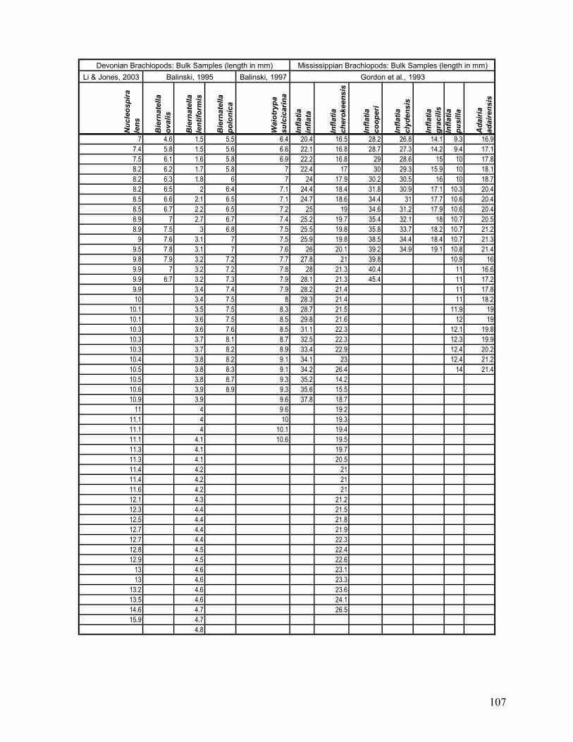
107
Li & Jones, 2003 Balinski, 1997
Nuc
leos
pira
le
ns
Bie
rnat
ella
ov
alis
Bie
rnat
ella
le
ntifo
rmis
Bie
rnat
ella
po
loni
ca
Wai
otry
pa
sulc
icar
ina
Infla
tia
infla
ta
Infla
tia
cher
okee
nsis
Infla
tia
coop
eri
Infla
tia
clyd
ensi
s
Infla
tia
grac
ilis
Infla
tia
pusi
lla
Ada
iria
adai
rens
is
7 4.6 1.5 5.5 6.4 20.4 16.5 28.2 26.8 14.1 9.3 16.97.4 5.8 1.5 5.6 6.6 22.1 16.8 28.7 27.3 14.2 9.4 17.17.5 6.1 1.6 5.8 6.9 22.2 16.8 29 28.6 15 10 17.88.2 6.2 1.7 5.8 7 22.4 17 30 29.3 15.9 10 18.18.2 6.3 1.8 6 7 24 17.9 30.2 30.5 16 10 18.78.2 6.5 2 6.4 7.1 24.4 18.4 31.8 30.9 17.1 10.3 20.48.5 6.6 2.1 6.5 7.1 24.7 18.6 34.4 31 17.7 10.6 20.48.5 6.7 2.2 6.5 7.2 25 19 34.6 31.2 17.9 10.6 20.48.9 7 2.7 6.7 7.4 25.2 19.7 35.4 32.1 18 10.7 20.58.9 7.5 3 6.8 7.5 25.5 19.8 35.8 33.7 18.2 10.7 21.2
9 7.6 3.1 7 7.5 25.9 19.8 38.5 34.4 18.4 10.7 21.39.5 7.8 3.1 7 7.6 26 20.1 39.2 34.9 19.1 10.8 21.49.8 7.9 3.2 7.2 7.7 27.8 21 39.8 10.9 169.9 7 3.2 7.2 7.8 28 21.3 40.4 11 16.69.9 6.7 3.2 7.3 7.9 28.1 21.3 45.4 11 17.29.9 3.4 7.4 7.9 28.2 21.4 11 17.810 3.4 7.5 8 28.3 21.4 11 18.2
10.1 3.5 7.5 8.3 28.7 21.5 11.9 1910.1 3.6 7.5 8.5 29.8 21.6 12 1910.3 3.6 7.6 8.5 31.1 22.3 12.1 19.810.3 3.7 8.1 8.7 32.5 22.3 12.3 19.910.3 3.7 8.2 8.9 33.4 22.9 12.4 20.210.4 3.8 8.2 9.1 34.1 23 12.4 21.210.5 3.8 8.3 9.1 34.2 26.4 14 21.410.5 3.8 8.7 9.3 35.2 14.210.6 3.9 8.9 9.3 35.6 15.510.9 3.9 9.6 37.8 18.7
11 4 9.6 19.211.1 4 10 19.311.1 4 10.1 19.411.1 4.1 10.6 19.511.3 4.1 19.711.3 4.1 20.511.4 4.2 2111.4 4.2 2111.6 4.2 2112.1 4.3 21.212.3 4.4 21.512.5 4.4 21.812.7 4.4 21.912.7 4.4 22.312.8 4.5 22.412.9 4.5 22.6
13 4.6 23.113 4.6 23.3
13.2 4.6 23.613.5 4.6 24.114.6 4.7 26.515.9 4.7
4.8
Mississippian Brachiopods: Bulk Samples (length in mm)Gordon et al., 1993
Devonian Brachiopods: Bulk Samples (length in mm)Balinski, 1995

108
Li & Jones, 2003 Balinski, 1997
Nuc
leos
pira
le
ns
Bie
rnat
ella
ov
alis
Bie
rnat
ella
le
ntifo
rmis
Bie
rnat
ella
po
loni
ca
Wai
otry
pa
sulc
icar
ina
Infla
tia
infla
ta
Infla
tia
cher
okee
nsis
Infla
tia
coop
eri
Infla
tia
clyd
ensi
s
Infla
tia
grac
ilis
Infla
tia
pusi
lla
Ada
iria
adai
rens
is
4.84.84.84.94.94.94.9
55.15.15.15.15.25.25.35.35.35.45.45.55.65.65.65.75.85.85.9
66
6.16.16.16.26.36.36.56.56.76.86.86.96.96.96.9
777
7.17.17.37.47.58.3
Balinski, 1995 Gordon et al., 1993Devonian Brachiopods: Bulk Samples (length in mm) Mississippian Brachiopods: Bulk Samples (length in mm)

109
Tere
brat
ulin
a w
ilson
i
Tere
brat
ulin
a la
chry
ma
Bas
iliol
a sp
.
Gira
liath
ryris
ju
bile
ensi
s
Vict
orith
yris
bl
akeo
rum
10 29.75 9.75 22 25 27.75 33 6.75 5.6 3.6 36.3 24.3 26.6 22.7 19.9 29.1 26.3 21.610.75 30 11.25 22 25 27.75 33 6.9 7.5 5.4 20.9 24.6 19.6 27.8 20 26.2 27.3 23
12.5 30 13.5 22.25 25.25 27.75 33 8.8 10.3 6 23.9 24.5 25.9 24.5 22.4 26.3 31.4 13.813.5 30 13.75 22.5 25.25 28 33 9.5 10.8 6.5 25.3 27.5 26.7 24.5 23.8 23.8 23.4 18.315.5 30.5 13.75 22.5 25.25 28 33.5 9.75 11.25 6.7 26.3 24.5 28.7 34.5 24.1 27.4 26.3 16.1
15.75 31 14.75 22.5 25.25 28 33.5 10 11.4 6.8 26.4 24.7 23 24.4 30.9 17.415.75 31 15.25 22.5 25.25 28 33.75 10.3 11.5 7.1 28.6 31.2 21.2 25.6 24.6 15.2
16 31.25 15.75 22.5 25.25 28 33.75 10.5 12.1 7.4 30.4 27.2 25.6 26.1 28.7 12.818 31.25 15.75 22.5 25.25 28.25 33.75 10.5 12.1 7.5 31 28.3 18.7 26.2 24.8 20.2
18.25 31.75 16 22.5 25.5 28.25 34 10.6 12.1 7.7 28 25.6 19.9 26.9 21.4 19.618.5 32.25 16.5 22.5 25.5 28.25 34 10.6 12.25 7.7 17.4 24.5 22.1 26.9 19.4 19.3
19.25 32.75 16.5 22.75 25.5 28.25 34 10.7 12.25 7.8 25 29.1 25.2 27.2 23.1 19.819.5 32.75 16.5 22.75 25.5 28.25 34.25 10.8 12.6 8 26 25 20.6 27.7 24.5 18.5
20.25 33 16.75 22.75 25.5 28.5 35.25 11 13.1 9.4 21.2 24.6 24.6 29.3 25.2 18.120.25 33 17 23 25.5 28.5 36 11 13.6 11.9 19.6 26.6 28.7 29.8 27.3 19.9
20.5 33 17.5 23 25.5 28.75 36 11.2 13.6 20.6 25 14.1 30.7 22.6 16.321 34.75 17.5 23 25.5 28.75 36 11.3 13.7 18 24.3 14.6 30.8 23 19.4
21.5 34.75 18.5 23 25.75 28.75 36.25 11.5 13.75 20.3 25.9 29.6 30.9 18.1 1721.75 35 18.75 23 25.75 28.75 36.5 11.75 13.8 26.2 17.2 20.7 31.1 29.2 17.521.75 35 19 23.25 25.75 29 37.5 11.8 14.6 27.5 24.2 19.5 31.2 23.5 19.721.75 35 19 23.25 25.75 29 38 11.8 14.6 28.6 19 19.4 31.7 30.2 18.8
22 36.25 19 23.25 25.75 29 38.75 11.8 15.5 20.4 16.9 15.6 31.8 16.3 20.722.25 36.25 19.25 23.25 25.75 29.25 39.25 12.4 15.6 17.8 18.9 25.5 31.9 35.1 18.822.75 37.25 19.5 23.25 26 29.25 39.5 12.4 15.75 24.8 21.2 22.6 32 27.6 16.522.75 37.5 19.75 23.25 26 29.25 39.5 12.4 27.9 24.6 19.3 32 30.3 18.7
23 38.5 19.75 23.25 26 29.5 41.5 12.5 23.5 33.8 25.8 32.3 33.2 17.523.25 38.5 19.75 23.25 26 29.75 41.75 12.5 25.1 28.8 25.5 32.6 26.3 20.823.75 38.75 19.75 23.5 26 29.75 12.75 22.6 29.1 23.8 33 25.3 17.6
24 39 19.75 23.5 26 30 12.75 22.2 26.9 24.4 33.5 26.8 18.124.25 39.75 19.75 23.5 26.5 30 12.75 18.5 15.1 24.5 33.6 24.6 18.2
24.5 40.25 20.25 23.5 26.5 30 12.75 18.7 20.1 28 33.9 25.3 19.424.75 20.75 23.75 26.5 30 13 16.4 19.1 26.3 34.3 25.3 18.424.75 20.75 23.75 26.5 30 13 13 23.9 34.5 26.8 17.924.75 21 23.75 26.75 30.5 13 15.2 25.2 34.6 29.5 17.2
25 21 24 26.75 30.75 13.2 15.4 26.7 35.4 28 19.725.75 21 24 26.75 31 13.3 14.4 23.8 35.7 23.4 11.5
26 21 24 27 31 13.3 13.7 24.7 36 26.3 11.126 21 24 27 31 13.5 13.1 34.4 36.3 29.1 16.726 21 24.25 27 31 13.6 20.4 26.9 36.6 24.9 23.5
26.25 21.25 24.25 27.25 31.25 13.75 22.4 32.6 37.1 27.126.25 21.5 24.25 27.25 31.25 13.75 18.9 25.6 38.3 28.826.75 21.5 24.5 27.25 31.25 13.9 27 19 39.6 19.927.25 21.5 24.5 27.25 31.75 14.1 25.1 20 16.3 22.727.25 21.75 24.5 27.5 31.75 14.1 29.5 27.6 10 23.627.25 21.75 24.5 27.75 31.75 14.1 25.1 31.8 29.127.75 21.75 24.5 27.75 31.75 14.4 19.1 27 31.227.75 21.75 24.5 27.75 32.25 14.4 23 19.5 25.1
28 21.75 25 27.75 32.25 14.4 28.9 25.2 27.329 22 25 27.75 32.25 24.2 23 28.9
Cooper, 1988 Craig, 2000Paleocene-Eocene Brachiopods: Bulk Samples (length in mm)
Vict
orith
yris
de
cape
llo
Plic
ator
ia
wilm
ingt
onen
sis
1
Plic
ator
ia
wilm
ingt
onen
sis
2
Gira
liath
yris
m
cnam
arai
Gira
liath
yris
ka
itrin
ae
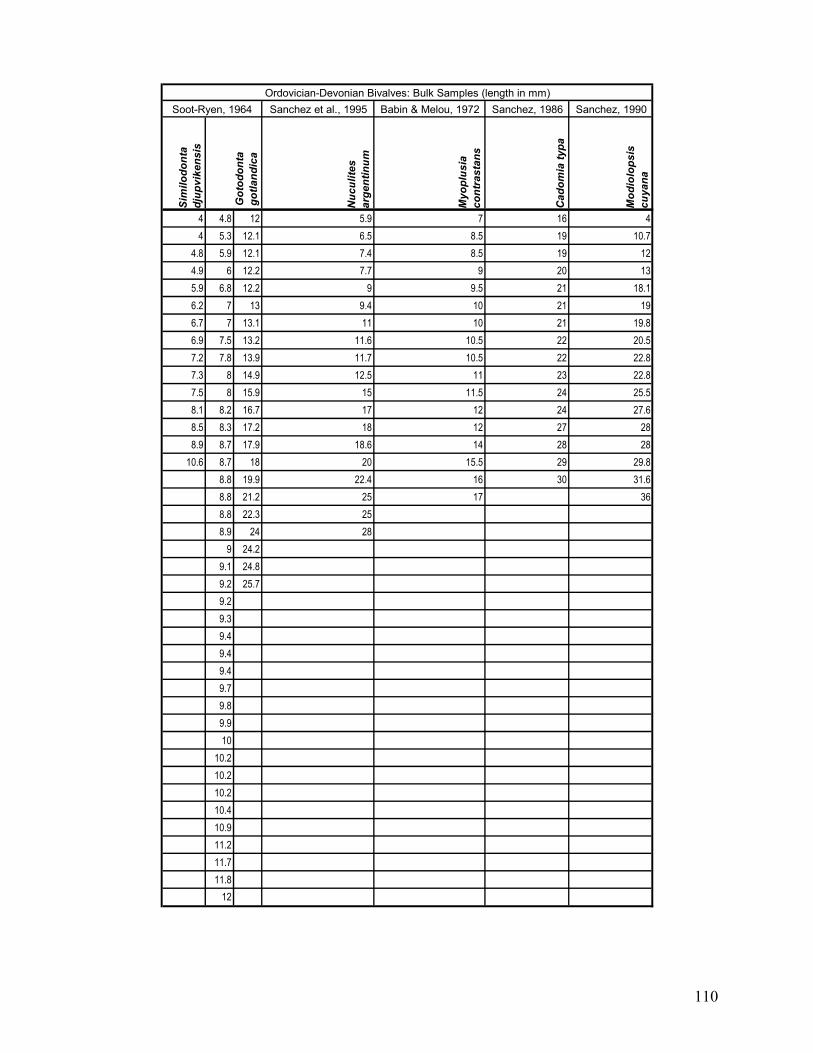
110
Sanchez et al., 1995 Babin & Melou, 1972 Sanchez, 1986 Sanchez, 1990
Sim
ilodo
nta
djup
vike
nsis
Nuc
ulite
s ar
gent
inum
Myo
plus
ia
cont
rast
ans
Cad
omia
typa
Mod
iolo
psis
cu
yana
4 4.8 12 5.9 7 16 44 5.3 12.1 6.5 8.5 19 10.7
4.8 5.9 12.1 7.4 8.5 19 124.9 6 12.2 7.7 9 20 135.9 6.8 12.2 9 9.5 21 18.16.2 7 13 9.4 10 21 196.7 7 13.1 11 10 21 19.86.9 7.5 13.2 11.6 10.5 22 20.57.2 7.8 13.9 11.7 10.5 22 22.87.3 8 14.9 12.5 11 23 22.87.5 8 15.9 15 11.5 24 25.58.1 8.2 16.7 17 12 24 27.68.5 8.3 17.2 18 12 27 288.9 8.7 17.9 18.6 14 28 28
10.6 8.7 18 20 15.5 29 29.88.8 19.9 22.4 16 30 31.68.8 21.2 25 17 368.8 22.3 258.9 24 28
9 24.29.1 24.89.2 25.79.29.39.49.49.49.79.89.910
10.210.210.210.410.911.211.711.8
12
Got
odon
ta
gotla
ndic
a
Soot-Ryen, 1964Ordovician-Devonian Bivalves: Bulk Samples (length in mm)

111
Jane
ia s
iluric
a
Myt
ilarc
a bl
oom
field
ensi
sC
orne
llite
s ca
tellu
sTo
lmai
a er
ugis
ulca
Gon
ioph
ora
dupl
isul
ca
Cyp
ricar
dini
a m
inim
a
Eosc
hizo
dus
taem
asen
sis
Cra
ssat
ello
psis
le
ntic
ular
is
2.8 7.5 11.2 1.7 6.5 10.3 11.7 3.5 0.9 9.1 8 10 12 5 1.6 12.5 6.52.8 7.5 11.2 1.7 6.5 10.3 11.7 5.25 1 9.2 13 12 15.5 5.25 1.9 12.5 6.753.1 7.7 11.2 2.2 6.5 10.3 11.7 6.75 1.3 10.2 15.5 13.5 20 8 2 15 83.1 7.7 11.3 2.2 6.5 10.3 11.7 6.75 1.3 11.1 16 14.5 22 10 2.1 17.5 8.253.3 7.9 11.3 2.3 6.7 10.4 11.8 7.5 1.7 11.8 17.5 16.5 23.5 10 2.4 18.5 9.53.4 9 11.3 2.3 6.7 10.5 11.9 11.75 1.7 11.8 19 18 24 11 2.6 18.5 9.53.5 9 11.3 2.5 6.8 10.6 11.9 12.75 2 11.9 20 22 29.5 12 2.7 19 113.5 9 11.5 2.5 6.8 10.6 11.9 15 2 12.3 20.5 22 30 12 2.9 20 113.5 9 11.5 2.7 7.4 10.6 11.9 15.1 2.3 12.7 25 24 41.5 12.5 3 22 11.53.5 9.1 11.6 2.7 7.6 10.6 11.9 16.25 2.3 12.8 26 25 41.5 14 3.2 22.5 11.753.6 9.3 11.6 3.6 7.6 10.8 11.9 17.5 2.8 12.9 27 28 46 14.5 3.75 23 12.253.8 9.3 11.6 3.6 7.7 10.8 11.9 17.5 2.8 12.9 32 38.5 50 15.5 3.8 24 143.8 9.4 11.7 3.6 7.8 10.8 12 17.9 2.8 13.2 32 40.5 57 17.25 3.8 26 14.53.9 9.4 11.8 3.8 8.1 10.8 12.1 18.1 3.1 13.7 46 58 17.5 4.8 26.5 16
4 9.5 11.8 3.8 8.3 10.8 12.1 19.9 3.2 14.6 66 18 5.1 174 9.6 11.9 4 8.4 10.9 12.2 20.1 3.2 70 18.5 5.2
4.1 9.6 12 4.2 8.5 10.9 12.3 23 3.2 19 5.24.1 9.7 12 4.2 8.7 10.9 12.3 28.75 3.3 19 5.64.2 9.7 12.1 4.3 8.8 10.9 12.3 3.5 19.254.2 9.8 12.1 4.3 8.8 10.9 12.4 3.7 19.54.5 9.8 12.1 4.3 8.9 11 12.5 4 204.5 9.8 12.1 4.4 8.9 11 12.5 4.1 20.254.8 9.9 12.2 4.4 8.9 11 12.5 4.4 20.754.8 10 12.2 4.5 9 11.1 12.6 4.6 214.9 10 12.2 4.5 9.1 11.1 12.8 4.6 22.54.9 10 12.3 4.6 9.1 11.2 12.9 4.7 26
5 10.1 12.3 4.6 9.3 11.3 12.9 4.85 10.1 12.5 4.7 9.3 11.3 12.9 5
5.2 10.1 12.5 4.7 9.3 11.3 13 5.25.3 10.1 12.6 5 9.4 11.3 13.1 5.35.6 10.2 12.8 5 9.4 11.3 13.1 5.55.6 10.3 12.8 5 9.4 11.3 13.2 5.65.8 10.3 12.8 5 9.6 11.4 13.2 5.85.8 10.3 12.8 5.1 9.6 11.4 13.2 6.55.8 10.3 13.2 5.4 9.6 11.4 13.5 6.55.8 10.3 13.5 5.4 9.7 11.5 13.5 6.7
6 10.3 14.4 5.5 9.7 11.5 13.7 6.86 10.6 14.4 5.5 9.7 11.5 13.8 7
6.2 10.7 14.4 5.5 9.7 11.5 13.8 7.26.2 10.7 14.4 5.5 9.8 11.6 14 7.36.5 10.7 14.6 5.6 9.8 11.6 14.1 7.46.7 10.9 14.7 5.7 9.9 11.7 14.2 7.86.7 10.9 14.8 5.7 10 11.7 14.4 86.8 10.9 15 5.8 10 11.7 14.5 8.2
7 10.9 5.9 10 11.7 14.6 8.47.1 11 5.9 10 11.7 14.7 8.47.3 11 6 10 11.7 14.7 8.97.4 11 6 10.1 11.7 14.7 97.4 11.1 6.5 10.1 11.7 15.3 9
15.3 9
Johnston, 1993Ordovician-Devonian Bivalves: Bulk Samples (length in mm)
Nuc
uloi
da le
ns
Nuc
ulod
onta
go
tland
ica
Liljedahl, 1983
Frej
a fe
cund
a
Liljedahl, 1984

112
Amano, 1986
Ana
dara
tr
ansv
ersa
1
Ana
dara
tr
ansv
ersa
2
Ana
dara
tr
ansv
ersa
3
Gly
cym
eris
id
ensi
s
Ast
arte
om
alii
omal
ii
Dig
itaria
di
gita
ria 2
Ast
arte
fusc
a in
cras
sata
10 27.8 15.2 28.6 10.75 8.75 13 16.8 13 6.25 14.4 17.1 5.45 8.38 4.68 6.03 5.1 7.510.3 28.9 18.4 29.3 11.6 8.75 13.25 16.8 13 7.6 14.5 17.25 5.67 8.39 4.82 5.99 5.39 9.510.6 30.5 19.1 29.4 18.2 8.75 13.3 16.9 16.7 7.9 14.5 17.5 5.97 8.51 4.89 6 5.48 10.511.3 31.2 24.6 33.8 19.8 9.25 13.3 16.9 16.8 8.9 14.5 17.75 5.87 8.51 4.9 5.97 5.51 10.512.9 31.3 26.4 30.5 21.6 9.25 13.4 16.9 22.3 10.25 14.5 17.75 6 8.83 4.86 6.1 5.61 11.5
13 32.1 28.6 36.8 22.4 9.5 13.4 17 20.6 10.3 14.7 17.9 6.06 8.68 5.12 6.17 5.61 11.513.5 33 29.4 32.6 22.5 9.5 13.6 17 20.7 10.3 14.7 17.9 6.11 8.7 5.16 5.94 5.66 12.5
14 33.6 29.5 31.8 23.5 9.75 13.6 17 21.1 10.6 14.9 18 6.09 8.57 4.93 6.05 5.66 12.514.4 33.8 36.6 28.3 23.6 9.75 13.75 17 10.75 14.9 18.4 6.19 8.7 5.35 6.4 5.68 12.514.6 34.5 37.4 33.8 23.6 10 13.8 17.25 11.1 14.9 18.7 6.19 8.69 5.42 5.89 5.69 12.514.6 35.5 40.7 36.4 23.6 10 13.9 17.25 11.25 14.9 14.4 6.25 8.77 5.33 5.99 5.7 13.514.6 35.5 42.7 35.2 23.8 10 14.2 17.4 11.3 15 14.4 6.43 9.03 5.3 6.05 5.72 13.514.7 36.1 44.8 33.4 24.5 10.25 14.5 17.4 11.6 15.1 14.4 6.37 9.08 5.46 5.75 13.5
15 36.6 45 33.3 24.9 10.25 14.5 17.4 11.6 15.25 17 6.31 9.2 5.33 5.77 13.515.1 37.7 47.4 30 25.1 10.25 14.6 17.4 11.8 15.25 17.1 6.39 9.31 5.42 5.78 13.515.2 38.1 49.1 34.4 27.4 10.25 14.6 17.5 11.9 15.25 17.1 6.52 9.35 5.52 5.78 13.515.4 38.4 50.1 29.4 28 10.25 14.7 17.5 11.9 15.4 6.61 9.59 5.64 5.78 13.515.5 40.7 52.7 38 28 10.5 14.8 17.6 12 15.5 6.79 9.73 5.17 5.8 14.515.5 41.3 53.6 27.4 28.5 10.5 14.9 17.6 12 15.6 6.55 9.8 5.24 5.8 14.515.6 42.6 54 26.1 29.4 10.5 14.9 17.7 12.1 15.6 6.36 9.87 5.33 5.84 14.5
16 31 30.4 10.75 14.9 17.7 12.25 15.6 6.32 9.91 5.33 5.85 14.516 29.4 30.5 10.75 14.9 17.75 12.4 15.6 6.49 10 5.36 5.86 14.5
16.2 28.8 31.5 10.8 15 17.75 12.4 15.7 6.46 10 5.37 5.9 14.516.3 28.1 32.4 10.8 15 17.75 12.6 15.7 6.76 10 5.4 5.91 14.516.3 29.5 33.3 10.8 15 17.75 12.6 15.8 6.7 10 5.46 5.92 14.516.5 36.4 33.75 11 15 17.75 12.7 15.8 6.65 10.2 5.49 5.93 14.516.6 34.7 36.5 11 15 17.75 12.75 15.8 6.86 10.3 5.46 5.96 14.517.2 25 36.6 11 15.1 17.75 12.75 15.8 6.94 10.4 5.51 5.97 14.517.4 34 36.9 11.1 15.3 17.9 12.8 15.8 6.91 10.5 5.56 5.98 14.517.5 29.4 11.1 15.5 17.9 12.8 15.9 6.87 10.5 5.52 5.99 14.5
18 28.9 11.25 15.5 17.9 13 15.9 6.88 10.7 5.59 6 14.518.1 31.3 11.5 15.9 18 13 16 7.03 10.8 5.58 6.04 14.518.2 32.5 11.5 15.9 18.2 13 16 7.05 10.8 5.55 6.07 15.518.2 30.3 11.75 15.9 18.2 13 16 7.18 11 5.6 6.09 15.518.2 26 11.75 15.9 18.2 13.2 16.1 7.4 11.2 5.59 6.11 15.518.3 30 11.8 16 18.25 13.25 16.1 7.79 11.3 5.68 6.15 15.518.9 35.7 11.8 16 18.25 13.25 16.2 7.03 11.4 5.68 6.19 15.519.1 35 11.9 16 18.4 13.4 16.2 7.1 12 5.62 6.24 15.519.1 34.3 11.9 16 18.6 13.4 16.2 7.29 13.3 5.7 15.519.5 31 11.9 16 18.75 13.4 16.4 7.74 12.5 5.64 15.519.5 33.5 11.9 16 18.9 13.4 16.4 7.35 13.3 5.71 15.5
20 32.7 12 16 19 13.5 16.4 7.2 8.11 5.63 15.520 33.1 12 16.1 19 13.5 16.4 7.19 8.2 5.61 15.520 32 12.25 16.1 19.4 13.6 16.5 7.27 8.32 5.63 15.520 35.8 12.25 16.1 19.4 13.6 16.5 7.52 5.66 16.5
20.3 34 12.3 16.2 19.5 13.75 16.5 7.51 5.74 16.520.4 32 12.3 16.2 19.5 13.75 16.5 8.05 5.74 16.520.5 27.5 12.3 16.3 19.6 13.8 16.5 7.95 5.81 16.520.9 29.8 12.5 16.3 19.8 13.9 16.7 7.58 5.89 16.5
21 30.4 12.5 16.3 19.8 13.9 16.7 7.64 5.86 17.522 12.6 16.5 19.8 14 16.7 7.82 5.8122 12.7 16.5 20 14 16.75 7.74 5.66
22.3 12.75 16.6 20 14 16.9 7.84 5.8222.5 12.9 16.6 20.25 14 16.9 8.34 5.92
13 16.6 20.25 14.2 16.9 8.13 5.9313 16.7 20.25 14.2 17 8.05 5.89
Ast
arte
sol
idul
a
Dig
itaria
di
gita
ria 1
Lauriat-Rage, 1982
Miocene-Pliocene Bivalves: Bulk Samples (length in mm)
Ast
arte
om
alii
scal
aris
1
Bird, 1965
Ast
arte
om
alii
scal
aris
2
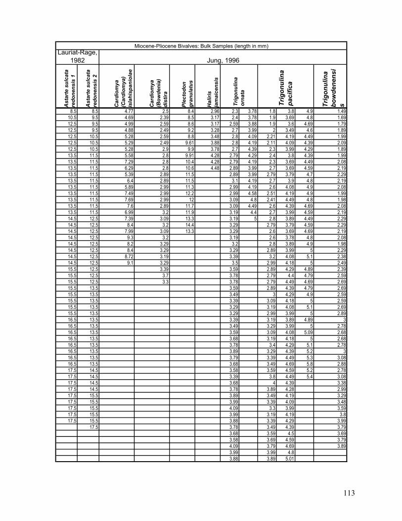
113
Ast
arte
sul
cata
re
done
nsis
1
Ast
arte
sul
cata
re
done
nsis
2
Car
diom
ya
(Car
diom
ya)
isla
hisp
anio
lae
Car
diom
ya
(Bow
deni
a)
dist
ira
Plec
todo
n gr
anul
atus
Hal
iris
jam
aice
nsis
Trig
onul
ina
bow
dene
nsi
s
8.5 8.5 4.77 2.5 8.4 2.96 2.3 3.78 1.8 3.8 4.9 1.4910.5 9.5 4.69 2.39 8.5 3.17 2.4 3.78 1.9 3.69 4.8 1.6912.5 9.5 4.99 2.59 8.6 3.17 2.59 3.88 1.9 3.6 4.69 1.7912.5 9.5 4.88 2.49 9.2 3.28 2.7 3.99 2 3.49 4.6 1.8912.5 10.5 5.28 2.59 8.8 3.48 2.8 4.09 2.21 4.19 4.49 1.9912.5 10.5 5.29 2.49 9.61 3.88 2.8 4.19 2.11 4.09 4.39 2.0912.5 10.5 5.28 2.9 9.9 3.78 2.7 4.39 2.3 3.99 4.29 1.8913.5 11.5 5.58 2.8 9.91 4.28 2.79 4.29 2.4 3.8 4.39 1.9913.5 11.5 7.29 2.8 10.4 4.28 2.79 4.19 2.3 3.69 4.49 2.0813.5 11.5 6.29 2.8 10.6 4.48 2.89 3.99 2.7 3.69 4.59 2.1913.5 11.5 5.39 2.89 11.5 2.89 3.99 2.79 3.79 4.7 2.2913.5 11.5 6.4 2.89 11.5 3.1 4.19 2.7 3.9 4.8 2.1913.5 11.5 5.89 2.99 11.3 2.99 4.19 2.6 4.08 4.9 2.0813.5 11.5 7.49 2.99 12.2 2.99 4.58 2.51 4.19 4.9 1.9913.5 11.5 7.69 2.99 12 3.09 4.8 2.41 4.49 4.8 1.9813.5 11.5 7.6 2.89 11.7 3.09 4.49 2.6 4.39 4.69 2.0813.5 11.5 6.99 3.2 11.9 3.19 4.4 2.7 3.99 4.59 2.1914.5 12.5 7.39 3.09 13.3 3.19 5 2.8 3.89 4.49 2.2914.5 12.5 8.4 3.2 14.4 3.29 2.79 3.79 4.59 2.2914.5 12.5 7.99 3.09 13.3 3.29 2.6 3.69 4.69 2.1914.5 12.5 9.3 3.2 3.19 2.6 3.78 4.8 2.0814.5 12.5 8.2 3.29 3.2 2.8 3.89 4.9 1.9814.5 12.5 8.4 3.29 3.29 2.89 3.99 5 2.2914.5 12.5 8.72 3.19 3.39 3.2 4.08 5.1 2.3814.5 12.5 9.1 3.29 3.5 2.99 4.18 5 2.4915.5 12.5 3.39 3.59 2.89 4.29 4.89 2.3915.5 12.5 3.7 3.78 2.79 4.4 4.79 2.5915.5 12.5 3.3 3.78 2.79 4.49 4.69 2.6915.5 13.5 3.59 2.89 4.39 4.79 2.6915.5 13.5 3.49 3 4.29 4.9 2.5915.5 13.5 3.39 3.09 4.18 5 2.5915.5 13.5 3.29 3.19 4.08 5.1 2.6915.5 13.5 3.29 2.99 3.99 5 2.8916.5 13.5 3.39 3.19 3.89 4.89 316.5 13.5 3.49 3.29 3.99 5 2.7816.5 13.5 3.59 3.09 4.08 5.09 2.6816.5 13.5 3.68 3.19 4.18 5 2.6816.5 13.5 3.78 3.4 4.29 5.1 2.7816.5 13.5 3.89 3.29 4.39 5.2 316.5 13.5 3.79 3.39 4.49 5.3 3.0816.5 13.5 3.68 3.49 4.69 5.8 2.8817.5 14.5 3.58 3.59 4.59 5.2 2.7817.5 14.5 3.39 3.8 4.49 5.4 3.0817.5 14.5 3.68 4 4.39 3.3817.5 14.5 3.78 3.89 4.28 2.9917.5 15.5 3.89 3.49 4.19 3.2917.5 15.5 3.99 3.39 4.09 3.4817.5 15.5 4.09 3.3 3.99 3.5917.5 15.5 3.99 3.19 4.19 3.817.5 15.5 3.88 3.39 4.29 3.99
17.5 3.78 3.49 4.39 3.793.68 3.59 4.5 3.693.58 3.69 4.59 3.794.09 3.79 4.69 3.893.99 3.99 4.83.88 3.89 5.01
Lauriat-Rage, 1982
Trig
onul
ina
orna
ta
Trig
onul
ina
paci
fica
Jung, 1996
Miocene-Pliocene Bivalves: Bulk Samples (length in mm)

114
Appendix 2.2: Monograph raw data
FIG
UR
ED
SP
EC
IME
NS
MA
GN
IFIC
ATI
ON
RA
W L
EN
GTH
(mm
)
CA
LIB
. LE
NG
TH (m
m)
RA
W W
IDTH
(mm
)
CA
LIB
. WID
TH (m
m)
PE
RC
EN
TILE
OF
BU
LK S
AM
PLE
(L
EN
GTH
)
Ordovician BrachiopodsAlberstadt, 1979Platystrophia annieana Plate 4:1 1.1 26.6 24.2 39.6 36.0 100USGS collection 7834-CO Plate 4:3 1.1 22.5 20.5 32.6 29.6 100
Plate 4:4 1.1 24.4 22.2 40.5 36.8 100Plate 4:5 1.1 21.4 19.5 30.0 27.3 96.5
Platystrophia colbienesis Plate 5:31 1.2 16.0 13.3 21.6 18.0 78.5USGS collection 7812-CO Plate 5:32 1.2 19.8 16.5 27.6 23.0 100
Plate 5:33 1.2 16.4 13.7 22.1 18.4 85Plate 5:34 1.2 14.1 11.8 19.3 16.1 71.5
Platystrophia elegantula Plate 5:70 1.2 12.5 10.4 17.1 14.3 10USGS collection 4982-CO
Platystrophia ponderosa Plate 2:22 1.1 30.9 28.1 40.6 36.9 64.5USGS collection 4556-CO Plate 2:23 1.1 27.6 25.1 38.5
Plate 2:24 1.1 21.7 19.7 29.3 26.6 3Plate 2:25 1.1 26.9 24.5 32.5Plate 2:26 1.1 26.4 24.0 34.5 31.4 32Plate 4:22 1.1 21.5 19.5 26.7 24.3 8Plate 4:23 1.1 13.6 12.4 17.4 15.8 1
Howe, 1979Sowerbyella sp. Plate 2:5 3 20.0 6.7 39.3 13.1 60.5USGS collection 8068-CO Plate 2:6 3 22.7 7.6 43.4 14.5 79
Plate 2:7 3 21.6 7.2 42.6 14.2 72Plate 2:11 3 34.0 11.3 72.2 24.1 100Plate 2:13 5 44.2 8.8 82.1 16.4 100
Rhyncotrema increbescens Plate 3:1 2.5 22.8 9.1 24.3 9.7 31.5USGS collection 5015-CO Plate 3:7 2.5 25.2 10.1 26.6 10.6 58.5
Plate 3:13 2.3 29.0 12.9 29.8 13.2 95Plate 3:18 2.3 29.1 12.9 33.8 15.0 96.5Plate 3:19 2.3 29.9 13.3 33.9 15.1 100Plate 3:22 3 33.4 11.1 32.0 10.7 65.5Plate 3:23 3 38.3 12.8 38.8 12.9 94
Orthorhynchula linneyi Plate 4:13 1.5 20.4 13.6 22.3 14.9 45USGS collection 6409-CO Plate 4:16 1.5 34.1 22.7 38.5 25.7 100
Plate 6:1 3 52.0 17.3 56.3 18.8 73

115
FIG
UR
ED
SP
EC
IME
NS
MA
GN
IFIC
ATI
ON
RA
W L
EN
GTH
(mm
)
CA
LIB
. LE
NG
TH (m
m)
RA
W W
IDTH
(mm
)
CA
LIB
. WID
TH (m
m)
PE
RC
EN
TILE
OF
BU
LK S
AM
PLE
(L
EN
GTH
)
Howe, 1979Orthorhynchula sublinneyi Plate 4:21 1.5 23.9 15.9 25.7 17.1 26USGS collection 5036-CO Plate 4:24 1.5 33.8 22.5 33.9 22.6 100USGS collection 5095-CO Plate 4:28 1.5 34.1 22.7 42.9 28.6 100
Plate 4:31 1.5 30.7 20.5 39.3 26.2 92.5Plate 5:11 3 43.3 14.4 60.3 20.1 16Plate 5:12 3 40.8 13.6 50.9 17.0 12.5Plate 5:15 3 55.8 18.6 69.3 23.1 81
Pope, 1979Oepikina minnesotensis Plate 1:2b 2 32.2 16.1 35.7 17.9 75.5USGS collection 5078-CO Plate 1:6b 2 34.6 17.3 39.6 19.8 91.5
Plate 1:7b 2 31.1 15.6 35.9 18.0 72.5Plate 1:8b 2 32.8 16.4 36.4 18.2 77Plate 1:9b 2 30.9 15.5 38.5 19.3 72.5Plate 1:10 2 31.2 15.6 37.2 18.6 73Plate 1:11b 2 27.5 13.8 30.5 15.3 40.5Plate 1:12b 2 27.2 13.6 32.3 16.2 40Plate 1:13 1 17.5 17.5 20.4 20.4 95Plate 1:14b 2 23.8 11.9 27.5 13.8 21Plate 2:1b 2 37.3 18.7 41.1 20.6 100Plate 2:2b 2 30.2 15.1 35.2 17.6 65Plate 2:3b 2 37.7 18.9 42.3 21.2 100Plate 2:4a 2 36.7 18.4 40.8 20.4 100Plate 2:7b 2 22.9 11.5 26.7 13.4 13.5Plate 2:8b 2 22.9 11.5 29.1 14.6 13.5Plate 2:9b 2 33.4 16.7 37.4 18.7 82Plate 3:9a 2 25.6 12.8 34.3 17.2 33Plate 3:10 2 25.2 12.6 30.9 15.5 28Plate 3:11 2 28.6 14.3 35.2 17.6 52Plate 3:13a 2 27.1 13.6 31.4 15.7 39.5Plate 3:14 2 24.6 12.3 28.7 14.4 25.5Plate 3:15 2 26.1 13.1 30.3 15.2 35Plate 3:17 2 30.1 15.1 34.3 17.2 64.5Plate 3:18 2 30.0 15.0 34.9 17.5 64.5Plate 3:19 2 29.1 14.6 35.9 18.0 57.5

116
FIG
UR
ED
SP
EC
IME
NS
MA
GN
IFIC
ATI
ON
RA
W L
EN
GTH
(mm
)
CA
LIB
. LE
NG
TH (m
m)
RA
W W
IDTH
(mm
)
CA
LIB
. WID
TH (m
m)
PE
RC
EN
TILE
OF
BU
LK S
AM
PLE
(L
EN
GTH
)
Oepikina minnesotensis Plate 1:1b 2 31.7 15.85 36.5 18.25 87USGS collection 7875-CO Plate 1:3b 2 33.1 16.55 32.8 16.4 92.5
Plate 1:4b 2 32.7 16.35 33.9 16.95 91Plate 1:5b 2 31.3 15.65 32.8 16.4 86Plate 2:5 2 30.8 15.4 38.9 19.45 81Plate 2:6 2 35.9 17.95 32.2 16.1 98.5Plate 3:1 2 30.3 15.15 35 17.5 78Plate 3:2 2 32.5 16.25 90.5Plate 3:3 2 30.3 15.15 37.7 18.85 78Plate 3:4 2 26.4 13.2 31.2 15.6 9.5Plate 3:5 2 30.1 15.05 35.6 17.8 77.5Plate 3:7 2 25.3 12.65 33.4 16.7 6Plate 3:8 2 29.6 14.8 35.7 17.85 65
Pionomena recens Plate 7:16 2.5 29.2 11.68 39.7 15.88 100USGS collection 5015-CO Plate 7:18 2.5 17.9 7.16 20.4 8.16 63.5
Plate 7:21a 2.5 18.2 7.28 23.5 9.4 64.5Plate 7:22a 2.5 20.5 8.2 27 10.8 84Plate 7:23 2.5 21.1 8.44 27.7 11.08 87.5Plate 7:24 2.5 25.5 10.2 34.6 13.84 98Plate 7:25 2.5 23.7 9.48 30.4 12.16 96Plate 7:26 2.5 18.5 7.4 25.8 10.32 68Plate 7:27 2.5 21.5 8.6 29.9 11.96 89Plate 7:20a 2.5 19 7.6 26.1 10.44 72
Silurian BrachiopodsAmsden, 1968Dicoelosia bilobella Fig. 3.6a USNM 158103 5 16.04 3.208 96St. Clair Limestone, Arkansas Fig. 3.6f USNM 158104 5 15.97 3.194 90
Fig. 8.2a USNM 158105 5 9.84 1.968 12Fig. 8.2c USNM 158106 5 15.21 3.042 84Fig. 8.2e USNM 158107 5 16.9 3.38 96
Dicoelosia oklahomensis Fig. 8.4a OU6283 5 15.01 3.002 61Henryhouse Fm., Oklahoma Fig. 8.4c OU6284 5 16.56 3.312 84
Fig. 8.4d OU6285 5 15.57 3.114 76

117
FIG
UR
ED
SP
EC
IME
NS
MA
GN
IFIC
ATI
ON
RA
W L
EN
GTH
(mm
)
CA
LIB
. LE
NG
TH (m
m)
RA
W W
IDTH
(mm
)
CA
LIB
. WID
TH (m
m)
PE
RC
EN
TILE
OF
BU
LK S
AM
PLE
(L
EN
GTH
)
Antirhynchonella thomasi Fig. 4.1d USNM 158137 2 16.47 8.235 17St. Clair Limestone, Arkansas Fig. 4.1e USNM 158138 2 20.34 10.17 55
Fig. 4.1i OU 6266 2 18.73 9.365 34Fig. 4.1k OU 6267 1 14.37 14.37 100Fig. 4.1l OU 6268 1 13.59 13.59 100Fig. 4.1r USNM 158139 2 20.95 10.475 62Fig. 4.1o USNM 158140 2 19 9.5 36Fig. 4.1s USNM 158143 2 17 8.5 23Fig. 4.1t USNM 158144 2 17.98 8.99 28
Hircinisca havliceki Fig. 5.5e USNM 158206 2 15.85 7.925 100St. Clair Limestone, Arkansas Fig. 5.5f USNM 158207 3 22.66 7.5533 82
Fig. 5.5k USNM 158208 3 23.29 7.7633 91Fig. 5.5n USNM 158209 3 17.11 5.7033 9
Eospirifer acutolineatus acutolineatus Fig. 1.1b USNM 158045 1 17.31 17.31 86St. Clair Limestone, Arkansas Fig. 1.1f USNM 158047 1 12.44 12.44 73
Fig. 1.1i USNM 158049 1 21.07 21.07 100Fig. 1.1l USNM 185050 2 20.79 10.395 42Fig. 1.1s USNM 158051 2 19.81 9.905 37
Eospirifer acutolineatus pentagonus Fig. 2.2a USNM 158059 1 17.97 17.97 74St. Clair Limestone, Arkansas Fig. 2.2d USNM 158060 1 19.43 19.43 87
Fig. 2.2e USNM 158061 1 18.06 18.06 74Fig. 2.2j USNM 158062 1 18.09 18.09 74Fig. 2.2k USNM 158063 1 19.58 19.58 87Fig. 2.2q USNM 158065 1 14.17 14.17 53.5
Kozlowskiellina (K.) vaningeni Fig. 2.1a USNM 158070 3 18.4 6.1333 9St. Clair Limestone, Arkansas Fig. 2.1e USNM 158071 3 20.01 6.67 20
Fig. 2.1f USNM 158072 3 21.55 7.1833 39Fig. 2.1l USNM 158073 3 14.9 4.9667 2.5Fig. 2.1q USNM 158075 1 11.69 11.69 93.5Fig. 2.1s USNM 158076 2 20.87 10.435 80.5
Atrypina erugata Fig. 10.4b USNM 158227 3 16.53 5.51 84.5St. Clair Limestone, Arkansas Fig. 10.4d USNM 158229 3 16.51 5.5033 84.5
Fig. 10.4o USNM 158231 4 21.29 5.3225 78.5Fig. 10.4h USNM 158232 3 18.92 6.3067 94.5Fig. 10.4n USNM 158233 3 24.95 8.3167 100
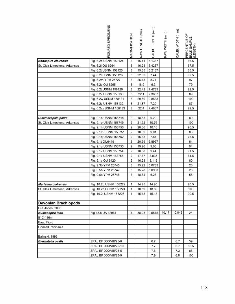
118
FIG
UR
ED
SP
EC
IME
NS
MA
GN
IFIC
ATI
ON
RA
W L
EN
GTH
(mm
)
CA
LIB
. LE
NG
TH (m
m)
RA
W W
IDTH
(mm
)
CA
LIB
. WID
TH (m
m)
PE
RC
EN
TILE
OF
BU
LK S
AM
PLE
(L
EN
GTH
)
Nanospira clairensis Fig. 6.2c USNM 158124 3 15.41 5.1367 65.5St. Clair Limestone, Arkansas Fig. 6.2i OU 6264 3 16.28 5.4267 67.5
Fig. 6.2j USNM 158125 3 15.65 5.2167 65.5Fig. 6.2l USNM 158126 3 22.32 7.44 92.5Fig. 6.2m YPM 25727 3 26.13 8.71 97Fig. 6.2s OU 6265 3 18.9 6.3 79Fig. 6.2t USNM 158129 3 22.42 7.4733 92.5Fig. 6.2v USNM 158130 3 22.1 7.3667 89Fig. 6.2w USNM 158131 3 29.59 9.8633 100Fig. 6.2y USNM 158132 3 21.87 7.29 87Fig. 6.2zz USNM 158133 3 22.4 7.4667 92.5
Dicamaropsis parva Fig. 9.1b USNM 158748 2 18.58 9.29 89St. Clair Limestone, Arkansas Fig. 9.1e USNM 158749 2 21.52 10.76 100
Fig. 9.1h USNM 158750 2 20.36 10.18 96.5Fig. 9.1m USNM 158751 2 18.02 9.01 86Fig. 9.1q USNM 158752 2 15.68 7.84 75.5Fig. 9.1t OU6419 3 20.69 6.8967 64Fig. 9.1u USNM 158753 2 19.26 9.63 94Fig. 9.1v USNM 158754 2 18.88 9.44 91.5Fig. 9.1x USNM 158755 2 17.67 8.835 84.5Fig. 9.1y OU 6420 2 16.23 8.115 80Fig. 9.3b YPM 25745 3 15.22 5.0733 26Fig. 9.5b YPM 25747 3 15.28 5.0933 26Fig. 9.6a YPM 25748 3 18.84 6.28 56
Meristina clairensis Fig. 10.2b USNM 158222 1 14.95 14.95 90.5St. Clair Limestone, Arkansas Fig. 10.2e USNM 158224 1 18.59 18.59 100
Fig. 10.2i USNM 158225 1 15.18 15.18 90.5
Devonian BrachiopodsLi & Jones, 2003Nucleospira lens Fig 13.8 UA 12961 4 38.23 9.5575 40.17 10.043 2481C-186mBaad FiordGrinnell Peninsula
Balinski, 1995Biernatella ovalis ZPAL BP XXXVIII/25-8 6.7 6.7 59
ZPAL BP XXXVIII/25-10 7.7 6.7 86.5ZPAL BP XXXVIII/25-5 7.6 7.3 86ZPAL BP XXXVIII/25-9 7.9 6.8 100

119
FIG
UR
ED
SP
EC
IME
NS
MA
GN
IFIC
ATI
ON
RA
W L
EN
GTH
(mm
)
CA
LIB
. LE
NG
TH (m
m)
RA
W W
IDTH
(mm
)
CA
LIB
. WID
TH (m
m)
PE
RC
EN
TILE
OF
BU
LK S
AM
PLE
(L
EN
GTH
)
Biernatella lentiformis ZPAL BP XXXVIII/32-76 5.8 5.7 73ZPAL BP XXXVIII/32-22 4.1 3.3 32ZPAL BP XXXVIII/32-85 6.5 6.2 84ZPAL BP XXXVIII/32-75 5.9 5.6 74ZPAL BP XXXVIII/32-97 8.4 8.8 100ZPAL BP XXXVIII/83 6.4 5.7 82.5ZPAL BP XXXVIII/32-81 6.2 6.2 80
Biernatella polonica ZPAL BP XXIII/30g 7 6.8 46
Balinski, 1997Waiotrypa sulcicarina GIUS 284/117 2 18.5 9.25 22.55 11.275 78
GIUS 284/122 2 19.79 9.895 24.25 12.125 91GIUS 284/121 2 18.69 9.345 24.24 12.12 83
Mississippian BrachiopodsGordon et al., 1993Inflatia inflata USNM 123977a 35.6 96NMNH loc. 568 USNM 123977b 37.8 98
Inflatia cherokeensis USNM 218947x 24.1 95NMNH loc. 568 & 569 CAS 6603.01 23 86
Inflatia cooperi USNM 218964 35.8 66NMNH loc. 469 USNM 218968 31.8 39
Inflatia clydensis USNM 218954 29.3 33USGS coll. 7088 USNM 218955 32.1 74
Inflatia gracilis USNM 218972 18 73NMNH loc. 568
Inflatia pusilla USNM 218981 10.9 54NMNH loc. 570
Adairia adairensis USNM 218966c 17.8 29NMNH loc. 566 & 568 USNM 218966a 21.2 87

120
FIG
UR
ED
SP
EC
IME
NS
MA
GN
IFIC
ATI
ON
RA
W L
EN
GTH
(mm
)
CA
LIB
. LE
NG
TH (m
m)
RA
W W
IDTH
(mm
)
CA
LIB
. WID
TH (m
m)
PE
RC
EN
TILE
OF
BU
LK S
AM
PLE
(L
EN
GTH
)
Paleocene-Eocene BrachiopodsCooper, 1988Plicatoria wilmingtonensis 2.21.USNM550866 1 27.33 27.33 56Wilmington, NC 2.28.USNM550870 1 32.36 32.36 74.5USGS loc. 3602 (North Carolina 1) 7.4.USNM549389i 1 39.5 39.5 98
7.5.USNM549389e 1 34.22 34.22 81.57.11.USNM549389-1 1 33.94 33.94 81.57.13.USNM549389c 1 33.95 33.95 81.57.20.USNM549389f 1 33.77 33.77 81.57.24.USNM549389d 1 36.86 36.86 90.58.2.USNM549389h 1 37.81 37.81 928.7.USNM550874 1 23.31 23.31 338.9.USNM549389k 1 33.73 33.73 81.59.9.USNM550877 1 15.48 15.48 69.15.USNM550865a 1 38.98 38.98 979.17.USNM550869 1 33.01 33.01 819.21.USNM550873 1 27 27 52.59.27.USNM551524 1 20.29 20.29 189.28.USNM550812 1 39.99 39.99 98.59.31.USNM548398n 1 25.77 25.77 449.33.USNM550876 1 43.6 43.6 1009.34.USNM550867 1 25.39 25.39 43.59.35.USNM550880 1 35.29 35.29 879.39.USNM550811 1 15.88 15.88 8.59.40.USNM550868 1 38.77 38.77 969.2.USNM550879 1 21.9 21.9 279.13.USNM550810a 1 13.61 13.61 4
Plicatoria wilmingtonensis 8.14.USNM551495a 1 31.37 31.37 84.5Ideal Cement Company Quarry 8.17.USNM551499 1 23.78 23.78 37Loc: North Carolina 2 8.21.USNM551502 1 30.81 30.81 81.5
8.22.USNM551494a 1 33.16 33.16 89.58.27.USNM551497a 1 32.45 32.45 878.29.USNM551496a 1 40.06 40.06 99.58.31.USNM551501 2 30.41 15.205 38.32.USNM551500 2 44.69 22.345 23.5
Terebratulina wilsoni 1.15.USNM551515a 3 41.57 13.857 86Loc.: South Carolina 4 6.29.USNM? 2 25.29 12.645 56.5
Terebratulina lachryma 1.16.USNM551516a 3 47.72 15.907 100Loc.: South Carolina 2

121
FIG
UR
ED
SP
EC
IME
NS
MA
GN
IFIC
ATI
ON
RA
W L
EN
GTH
(mm
)
CA
LIB
. LE
NG
TH (m
m)
RA
W W
IDTH
(mm
)
CA
LIB
. WID
TH (m
m)
PE
RC
EN
TILE
OF
BU
LK S
AM
PLE
(L
EN
GTH
)
Craig, 2000Basiliola sp. 1.10.WAM84.588c 3.8 27.53 7.3413 47Upper Paleocene 1.12.WAM84.588a 4 35.16 8.79 86.5
1.15.WAM84.584 4 30.73 7.6825 61
Giraliathyris mcnamarai 2.3.WAM96.826 3 71.22 23.74 41.5Upper Paleocene
Giraliathyris kaitrinae 3.2.WAM84.547 2 54.91 27.455 82Upper Paleocene 3.4.WAM96.609 2.6 54.37 20.912 25.5
Giraliathryris jubileensis 2.6.WAM84603e 2 74.84 37.42 95Middle Eocene 2.7.WAM84.604e 2 72.12 36.06 88.5
3.1.WAM84.604i 2 54.81 27.405 31.5
Victorithyris decapello 3.9.WAM96.645 2 59.92 29.96 87.5Upper Paleocene 4.2.WAM96.607 2 60 30 87.5
Victorithyris blakeorum 4.3.WAM96.706 2.5 54.64 21.856 94Upper Paleocene 4.5.WAM96.697 2.5 52.12 20.848 92
4.7.WAM88.111b 2.5 54.96 21.984 944.9.WAM88.111a 2.5 61.01 24.404 100
Ordovician-Devonian BivalvesSoot-Ryen, 1964Similodonta djupvikensis MO 21934 10.7 100Middle Silurian
Gotodonta gotlandica MO 150371 23.5 94Middle Silurian MO 150774 23.2 94
MO 150236 11.8 62MO 14988 8.6 21
Sanchez et al., 1995Nuculites argentinum 3.11.CORD-PZ8687 2 50.1 25.05 94Late Silurian - Early Devonian 3.12.CEGH-UNC1449 2 37.99 18.995 73
3.13.CORD-PZ8689 2.5 48.44 19.376 743.15.CEGH-UNC1441 1.5 34.2 22.8 843.16.CEGH-UNC1451 3 31.58 10.527 323.17.CORD-PZ8901 5.5 38.21 6.9473 10.53.19.CEGH-UNC1446 2 31.69 15.845 57.5
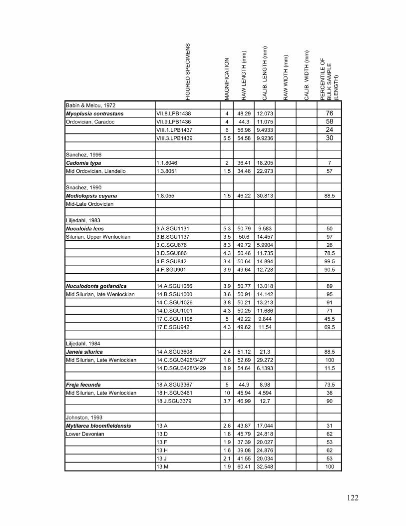
122
FIG
UR
ED
SP
EC
IME
NS
MA
GN
IFIC
ATI
ON
RA
W L
EN
GTH
(mm
)
CA
LIB
. LE
NG
TH (m
m)
RA
W W
IDTH
(mm
)
CA
LIB
. WID
TH (m
m)
PE
RC
EN
TILE
OF
BU
LK S
AM
PLE
(L
EN
GTH
)
Babin & Melou, 1972Myoplusia contrastans VII.8.LPB1438 4 48.29 12.073 76Ordovician, Caradoc VII.9.LPB1436 4 44.3 11.075 58
VIII.1.LPB1437 6 56.96 9.4933 24VIII.3.LPB1439 5.5 54.58 9.9236 30
Sanchez, 1996Cadomia typa 1.1.8046 2 36.41 18.205 7Mid Ordovician, Llandeilo 1.3.8051 1.5 34.46 22.973 57
Snachez, 1990Modiolopsis cuyana 1.8.055 1.5 46.22 30.813 88.5Mid-Late Ordovician
Liljedahl, 1983Nuculoida lens 3.A.SGU1131 5.3 50.79 9.583 50Silurian, Upper Wenlockian 3.B.SGU1137 3.5 50.6 14.457 97
3.C.SGU876 8.3 49.72 5.9904 263.D.SGU886 4.3 50.46 11.735 78.54.E.SGU842 3.4 50.64 14.894 99.54.F.SGU901 3.9 49.64 12.728 90.5
Nuculodonta gotlandica 14.A.SGU1056 3.9 50.77 13.018 89Mid Silurian, late Wenlockian 14.B.SGU1000 3.6 50.91 14.142 95
14.C.SGU1026 3.8 50.21 13.213 9114.D.SGU1001 4.3 50.25 11.686 7117.C.SGU1198 5 49.22 9.844 45.517.E.SGU942 4.3 49.62 11.54 69.5
Liljedahl, 1984Janeia silurica 14.A.SGU3608 2.4 51.12 21.3 88.5Mid Silurian, Late Wenlockian 14.C.SGU3426/3427 1.8 52.69 29.272 100
14.D.SGU3428/3429 8.9 54.64 6.1393 11.5
Freja fecunda 18.A.SGU3367 5 44.9 8.98 73.5Mid Silurian, Late Wenlockian 18.H.SGU3461 10 45.94 4.594 36
18.J.SGU3379 3.7 46.99 12.7 90
Johnston, 1993Mytilarca bloomfieldensis 13.A 2.6 43.87 17.044 31Lower Devonian 13.D 1.8 45.79 24.818 62
13.F 1.9 37.39 20.027 5313.H 1.6 39.08 24.876 6213.J 2.1 41.55 20.034 5313.M 1.9 60.41 32.548 100
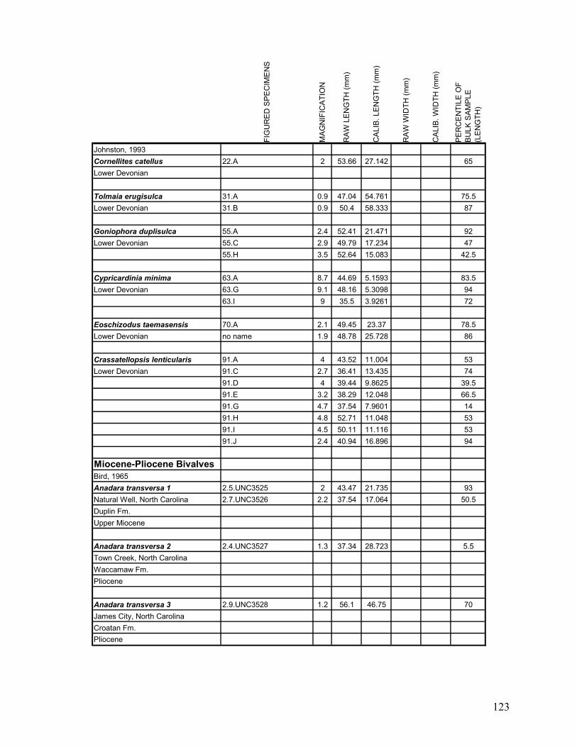
123
FIG
UR
ED
SP
EC
IME
NS
MA
GN
IFIC
ATI
ON
RA
W L
EN
GTH
(mm
)
CA
LIB
. LE
NG
TH (m
m)
RA
W W
IDTH
(mm
)
CA
LIB
. WID
TH (m
m)
PE
RC
EN
TILE
OF
BU
LK S
AM
PLE
(L
EN
GTH
)
Johnston, 1993Cornellites catellus 22.A 2 53.66 27.142 65Lower Devonian
Tolmaia erugisulca 31.A 0.9 47.04 54.761 75.5Lower Devonian 31.B 0.9 50.4 58.333 87
Goniophora duplisulca 55.A 2.4 52.41 21.471 92Lower Devonian 55.C 2.9 49.79 17.234 47
55.H 3.5 52.64 15.083 42.5
Cypricardinia minima 63.A 8.7 44.69 5.1593 83.5Lower Devonian 63.G 9.1 48.16 5.3098 94
63.I 9 35.5 3.9261 72
Eoschizodus taemasensis 70.A 2.1 49.45 23.37 78.5Lower Devonian no name 1.9 48.78 25.728 86
Crassatellopsis lenticularis 91.A 4 43.52 11.004 53Lower Devonian 91.C 2.7 36.41 13.435 74
91.D 4 39.44 9.8625 39.591.E 3.2 38.29 12.048 66.591.G 4.7 37.54 7.9601 1491.H 4.8 52.71 11.048 5391.I 4.5 50.11 11.116 5391.J 2.4 40.94 16.896 94
Miocene-Pliocene BivalvesBird, 1965Anadara transversa 1 2.5.UNC3525 2 43.47 21.735 93Natural Well, North Carolina 2.7.UNC3526 2.2 37.54 17.064 50.5Duplin Fm.Upper Miocene
Anadara transversa 2 2.4.UNC3527 1.3 37.34 28.723 5.5Town Creek, North CarolinaWaccamaw Fm.Pliocene
Anadara transversa 3 2.9.UNC3528 1.2 56.1 46.75 70James City, North CarolinaCroatan Fm.Pliocene
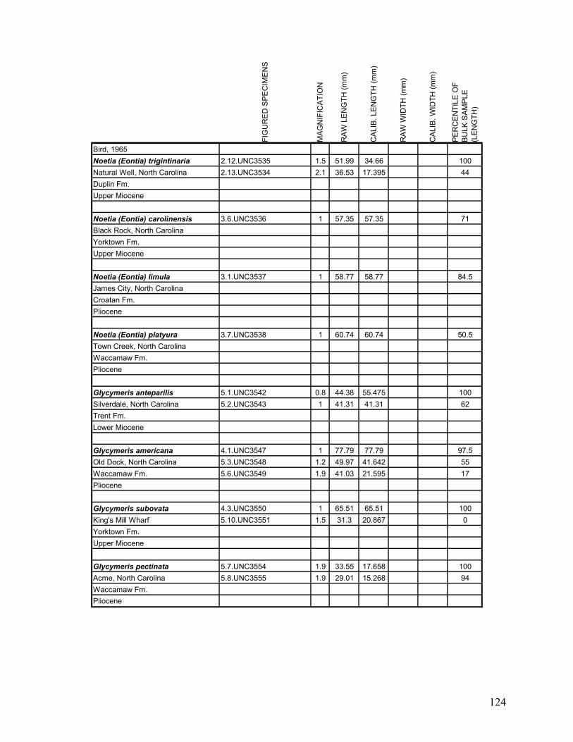
124
FIG
UR
ED
SP
EC
IME
NS
MA
GN
IFIC
ATI
ON
RA
W L
EN
GTH
(mm
)
CA
LIB
. LE
NG
TH (m
m)
RA
W W
IDTH
(mm
)
CA
LIB
. WID
TH (m
m)
PE
RC
EN
TILE
OF
BU
LK S
AM
PLE
(L
EN
GTH
)
Bird, 1965Noetia (Eontia) trigintinaria 2.12.UNC3535 1.5 51.99 34.66 100Natural Well, North Carolina 2.13.UNC3534 2.1 36.53 17.395 44Duplin Fm.Upper Miocene
Noetia (Eontia) carolinensis 3.6.UNC3536 1 57.35 57.35 71Black Rock, North CarolinaYorktown Fm.Upper Miocene
Noetia (Eontia) limula 3.1.UNC3537 1 58.77 58.77 84.5James City, North CarolinaCroatan Fm.Pliocene
Noetia (Eontia) platyura 3.7.UNC3538 1 60.74 60.74 50.5Town Creek, North CarolinaWaccamaw Fm.Pliocene
Glycymeris anteparilis 5.1.UNC3542 0.8 44.38 55.475 100Silverdale, North Carolina 5.2.UNC3543 1 41.31 41.31 62Trent Fm.Lower Miocene
Glycymeris americana 4.1.UNC3547 1 77.79 77.79 97.5Old Dock, North Carolina 5.3.UNC3548 1.2 49.97 41.642 55Waccamaw Fm. 5.6.UNC3549 1.9 41.03 21.595 17Pliocene
Glycymeris subovata 4.3.UNC3550 1 65.51 65.51 100King's Mill Wharf 5.10.UNC3551 1.5 31.3 20.867 0Yorktown Fm.Upper Miocene
Glycymeris pectinata 5.7.UNC3554 1.9 33.55 17.658 100Acme, North Carolina 5.8.UNC3555 1.9 29.01 15.268 94Waccamaw Fm.Pliocene
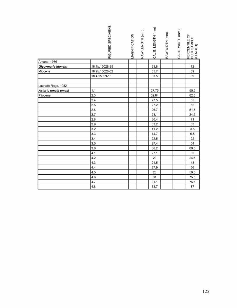
125
FIG
UR
ED
SP
EC
IME
NS
MA
GN
IFIC
ATI
ON
RA
W L
EN
GTH
(mm
)
CA
LIB
. LE
NG
TH (m
m)
RA
W W
IDTH
(mm
)
CA
LIB
. WID
TH (m
m)
PE
RC
EN
TILE
OF
BU
LK S
AM
PLE
(L
EN
GTH
)
Amano, 1986Glycymeris idensis 18.1b.15028-25 33.8 72Miocene 18.2b.15028-52 35.7 89
18.4.15029-15 33.5 69
Lauriate-Rage, 1982Astarte omalii omalii 1.1 27.75 55.5Pliocene 2.3 32.84 82.5
2.4 27.5 552.5 27.2 522.6 26.7 51.52.7 23.1 24.52.8 30.4 712.9 33.2 833.2 11.2 3.53.3 14.7 6.53.4 22.5 223.5 27.4 543.6 36.2 89.54.1 27.1 524.2 23 24.54.3 24.5 434.4 27.9 564.5 28 59.54.6 31 75.54.7 31.1 75.54.8 33.7 87

126
FIG
UR
ED
SP
EC
IME
NS
MA
GN
IFIC
ATI
ON
RA
W L
EN
GTH
(mm
)
CA
LIB
. LE
NG
TH (m
m)
RA
W W
IDTH
(mm
)
CA
LIB
. WID
TH (m
m)
PE
RC
EN
TILE
OF
BU
LK S
AM
PLE
(L
EN
GTH
)
Lauriat-Rage, 1982 1.3 19.4 91Astarte omalii scalaris 1 7.4 12.1 24.5(Nantes, France) 7.5 12.1 24.5
7.6 13.7 387.7 16.6 63.57.8 16.8 66.57.9 19.1 907.10 19.6 937.11 20.6 987.12 20.8 98.57.13 18.9 897.14 16.3 60.57.15 16.6 63.58.1 12.9 318.2 12.1 24.58.3 16.1 57.58.4 18.2 858.5 20.7 988.6 13.1 33.58.7 12.9 30.58.8 12.4 27.58.9 18.9 898.10 17.4 73.58.12 15.1 48.58.13 21 99

127
FIG
UR
ED
SP
EC
IME
NS
MA
GN
IFIC
ATI
ON
RA
W L
EN
GTH
(mm
)
CA
LIB
. LE
NG
TH (m
m)
RA
W W
IDTH
(mm
)
CA
LIB
. WID
TH (m
m)
PE
RC
EN
TILE
OF
BU
LK S
AM
PLE
(L
EN
GTH
)
Lauriat-Rage, 1982Astarte omalii scalaris 2 1.4 15.5 60(Angers, France) 5.2 10.4 5.5
5.3 10.6 65.4 13.5 335.5 16.1 73.55.6 15.6 625.7 18.2 98.55.8 18.3 98.55.9 16.3 76.55.10 14.2 435.11 16.2 75.55.12 15.5 605.13 13.1 26.55.14 16 71.55.15 14 415.17 17 906.1 16.7 84.56.2 17 906.3 14.9 53.56.4 14.9 53.56.5 18 986.6 14.8 51.56.8 11.4 96.9 13.2 276.10 15.7 646.11 16.7 84.56.12 17 906.13 16.5 80.56.14 18.7 1006.15 13.5 336.16 15.7 646.17 15.5 606.18 15.8 66.5
Astarte solidula 10.1 16.21 10010.2 14.25 10010.3 11.98 96.510.4 12.37 9710.5 13.2 98.5
Digitaria digitaria 1 14.13 5.9567 85.5le Pigeon-Blanc 14.14 6.36 99

128
FIG
UR
ED
SP
EC
IME
NS
MA
GN
IFIC
ATI
ON
RA
W L
EN
GTH
(mm
)
CA
LIB
. LE
NG
TH (m
m)
RA
W W
IDTH
(mm
)
CA
LIB
. WID
TH (m
m)
PE
RC
EN
TILE
OF
BU
LK S
AM
PLE
(L
EN
GTH
)
Lauriat-Rage, 1982 14.15 4.6767 0Digitaria digitaria 2la Gauviniere
Astarte fusca incrassata 1.5 16.13 88.5St. Michel 10.13 14.78 63.5
10.14 14.96 6410.15 17.83 10010.16 15.65 87.510.17 15.34 64.5
Astarte sulcata redonensis 1 1.6 16.17 66St. Michel 11.7 16.15 66
11.8 16.8 81.511.9 15.82 65.5
Astarte sulcata redonensis 2 11.21 15.58 98le Houx
Jung, 1996Cardiomya (Cardiomya) islahispaniolae 1.1 9.3 5.4 98.5late Miocene 1.3 8.4 5.2 84Dominican Republic 1.4 8.7 5.8 90
1.6 7.6 4.8 662.1 5 2.9 15.52.3 8 5.3 75.5
Cardiomya (Bowdenia) distira 3.5 3.2 2 73late Miocene - middle Pliocene 4.1 3 2 57Dominican Republic 4.3 2.9 2.3 44.5
4.4 3.3 2.3 91
Plectodon granulatus 2.9 11.3 6.7 52.5Recent 5.1 10.6 6.4 47.5Carribbean 6.1 8.8 5.6 17.5
6.3 11.5 6.5 60
Haliris jamaicensis 9.1 4.3 4.1 81Pliocene 9.4 4.3 3.9 81Dominican Republic 10.1 3.2 2.6 29.5
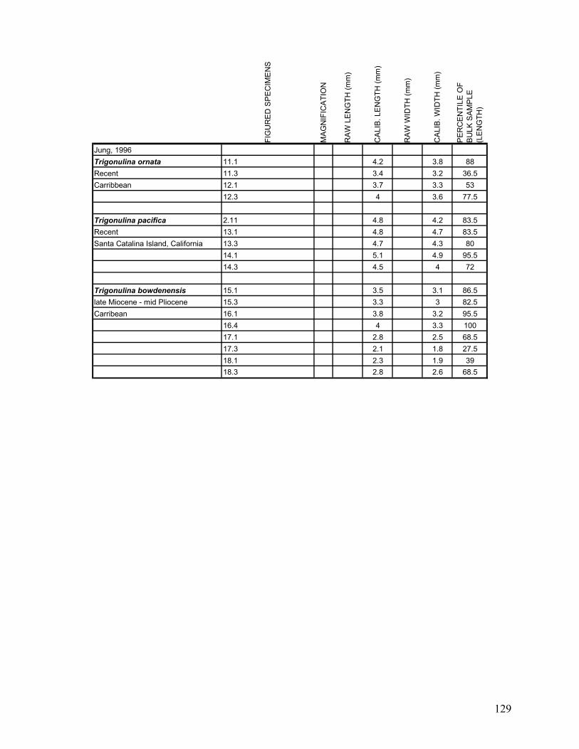
129
FIG
UR
ED
SP
EC
IME
NS
MA
GN
IFIC
ATI
ON
RA
W L
EN
GTH
(mm
)
CA
LIB
. LE
NG
TH (m
m)
RA
W W
IDTH
(mm
)
CA
LIB
. WID
TH (m
m)
PE
RC
EN
TILE
OF
BU
LK S
AM
PLE
(L
EN
GTH
)
Jung, 1996Trigonulina ornata 11.1 4.2 3.8 88Recent 11.3 3.4 3.2 36.5Carribbean 12.1 3.7 3.3 53
12.3 4 3.6 77.5
Trigonulina pacifica 2.11 4.8 4.2 83.5Recent 13.1 4.8 4.7 83.5Santa Catalina Island, California 13.3 4.7 4.3 80
14.1 5.1 4.9 95.514.3 4.5 4 72
Trigonulina bowdenensis 15.1 3.5 3.1 86.5late Miocene - mid Pliocene 15.3 3.3 3 82.5Carribean 16.1 3.8 3.2 95.5
16.4 4 3.3 10017.1 2.8 2.5 68.517.3 2.1 1.8 27.518.1 2.3 1.9 3918.3 2.8 2.6 68.5
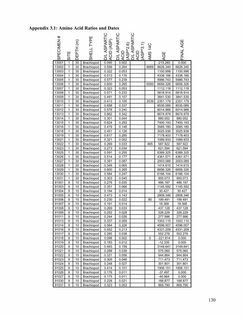
130
Appendix 3.1: Amino Acid Ratios and Dates
SPEC
IMEN
#
SITE
DEP
TH (m
)
SHEL
L TY
PE
D/L
ASP
ARTI
C
ACID
(ASP
)
D/L
ASP
ARTI
C
ACID
(A
SP^2
.6)
D/L
ASP
ARTI
C
ACID
(A
SP^3
.1)
AMS
14C
AGE
FIN
AL A
GE
13001 1 30 Brachiopod 0.095 0.002 -215.265 0.00013002 1 30 Brachiopod 0.599 0.264 6669 6626.340 6626.34013003 1 30 Brachiopod 0.322 0.053 1100.998 1100.99813004 1 30 Brachiopod 0.513 0.176 4338.166 4338.16613005 1 30 Brachiopod 0.577 0.239 5986.743 5986.74313006 1 30 Brachiopod 0.600 0.265 6550 6656.326 6656.32613007 1 30 Brachiopod 0.323 0.053 1112.118 1112.11813008 1 30 Brachiopod 0.571 0.233 5818.914 5818.91413009 1 30 Brachiopod 0.491 0.157 3841.530 3841.53013010 1 30 Brachiopod 0.413 0.100 2539 2351.179 2351.17913011 1 30 Brachiopod 0.658 0.337 8535.089 8535.08913012 1 30 Brachiopod 0.578 0.240 6014.988 6014.98813013 1 30 Brachiopod 0.662 0.342 8674.979 8674.97913014 1 30 Brachiopod 0.301 0.044 880.052 880.05213015 1 30 Brachiopod 0.624 0.293 7400.193 7400.19313016 1 30 Brachiopod 0.479 0.148 3585.180 3585.18013018 1 30 Brachiopod 0.451 0.126 3025.936 3025.93613019 1 30 Brachiopod 0.617 0.285 7178.403 7178.40313021 1 30 Brachiopod 0.321 0.052 1089.933 1089.93313022 1 30 Brachiopod 0.269 0.033 465 587.922 587.92213023 1 30 Brachiopod 0.273 0.034 621.594 621.59413025 1 30 Brachiopod 0.591 0.255 6389.325 6389.32513026 1 30 Brachiopod 0.514 0.177 4361.571 4361.57113027 1 30 Brachiopod 0.391 0.087 2003.089 2003.08913028 1 30 Brachiopod 0.349 0.065 1414.615 1414.61513029 1 30 Brachiopod 0.600 0.265 6656.326 6656.32613030 1 30 Brachiopod 0.584 0.247 6186.104 6186.10413031 1 30 Brachiopod 0.303 0.045 900.073 900.07391001 9 10 Brachiopod 0.276 0.035 486.197 486.19791003 9 10 Brachiopod 0.351 0.066 1145.592 1145.59291004 9 10 Brachiopod 0.194 0.014 30.427 30.42791005 9 10 Brachiopod 0.473 0.143 2808.346 2808.34691006 9 10 Brachiopod 0.230 0.022 80 199.491 199.49191007 9 10 Brachiopod 0.191 0.014 18.368 18.36891008 9 10 Brachiopod 0.269 0.033 437.128 437.12891009 9 10 Brachiopod 0.252 0.028 326.229 326.22991011 9 10 Brachiopod 0.244 0.026 277.996 277.99691013 9 10 Brachiopod 0.337 0.059 1003.110 1003.11091014 9 10 Brachiopod 0.564 0.226 4596.007 4596.00791016 9 10 Brachiopod 0.552 0.213 4331.209 4331.20991017 9 10 Brachiopod 0.285 0.038 552.276 552.27691018 9 10 Brachiopod 0.098 0.002 0 -221.814 0.00091019 9 10 Brachiopod 0.183 0.012 -12.335 0.00091020 9 10 Brachiopod 0.493 0.159 3149.641 3149.64191021 9 10 Brachiopod 0.288 0.039 575.060 575.06091022 9 10 Brachiopod 0.331 0.056 944.864 944.86491023 9 10 Brachiopod 0.305 0.046 711.473 711.47391024 9 10 Brachiopod 0.248 0.027 301.801 301.80191025 9 10 Brachiopod 0.414 0.101 1906.151 1906.15191026 9 10 Brachiopod 0.176 0.011 -37.497 0.00091027 9 10 Brachiopod 0.175 0.011 -40.964 0.00091030 9 10 Brachiopod 0.228 0.021 188.877 188.87791031 9 10 Brachiopod 0.323 0.053 869.790 869.790

131
SPEC
IMEN
#
SITE
DEP
TH (m
)
SHEL
L TY
PE
D/L
ASP
ARTI
C
ACID
(ASP
)
D/L
ASP
ARTI
C
ACID
(A
SP^2
.6)
D/L
ASP
ARTI
C
ACID
(A
SP^3
.1)
AMS
14C
AGE
FIN
AL A
GE
91032 9 10 Brachiopod 0.534 0.196 3825 3950.948 3950.94891033 9 10 Brachiopod 0.283 0.038 537.298 537.29891034 9 10 Brachiopod 0.443 0.120 2325.630 2325.63091036 9 10 Brachiopod 0.191 0.014 18.368 18.36891038 9 10 Brachiopod 0.398 0.091 1693.876 1693.876BB-1 9 10 Brachiopod 0.066 0.001 -254.517 0.000BB-2 9 10 Brachiopod 0.109 0.003 -205.815 0.000BB-3 9 10 Brachiopod 0.063 0.001 -257.009 0.000BB-4 9 10 Brachiopod 0.098 0.002 -221.486 0.000BB-5 9 10 Brachiopod 0.048 0.000 -265.056 0.000BB-6 9 10 Brachiopod 0.291 0.040 597.303 597.303BB-7 9 10 Brachiopod 0.060 0.001 -258.720 0.000BB-8 9 10 Brachiopod 0.170 0.010 -58.650 0.000BB-9 9 10 Brachiopod 0.062 0.001 -257.544 0.000BB-10 9 10 Brachiopod 0.044 0.000 -266.871 0.000BB-11 9 10 Brachiopod 0.120 0.004 -186.092 0.000BB-12 9 10 Brachiopod 0.248 0.027 304.678 304.678BB-13 9 10 Brachiopod 0.226 0.021 176.001 176.001BB-14 9 10 Brachiopod 0.438 0.117 2522 2251.313 2251.313BB-15 9 10 Brachiopod 0.340 0.061 784 1035.209 1035.209BB-16 9 10 Brachiopod 0.289 0.040 585.540 585.540301 9 10 Brachiopod 0.416 0.102 1938.357 1938.357376 9 10 Brachiopod 0.459 0.132 2576.398 2576.398442 9 10 Brachiopod 0.239 0.024 248.093 248.093543 9 10 Brachiopod 0.426 0.108 2067.954 2067.954546 9 10 Brachiopod 0.456 0.130 2532.186 2532.186594 9 10 Brachiopod 0.144 0.007 -132.582 0.0002 9 10 Brachiopod 0.132 0.005 -161.230 0.0003 9 10 Brachiopod 0.449 0.125 2423.188 2423.1884 9 10 Brachiopod 0.225 0.021 173.640 173.64020 9 10 Brachiopod 0.457 0.131 2549.953 2549.953
158 9 10 Brachiopod 0.241 0.025 259.521 259.521228 9 10 Brachiopod 0.269 0.033 439.144 439.144230 9 10 Brachiopod 0.240 0.024 254.957 254.957236 9 10 Brachiopod 0.333 0.057 965.218 965.218280 9 10 Brachiopod 0.455 0.129 2505.326 2505.326281 9 10 Brachiopod 0.490 0.156 3097.634 3097.634
13050 1 30 Bivalve 0.424 0.070 10761.275 10761.27513051 1 30 Bivalve 0.235 0.011 1641.822 1641.82213052 1 30 Bivalve 0.308 0.026 3917.733 3917.73313053 1 30 Bivalve 0.101 0.001 25.519 25.51913054 1 30 Bivalve 0.178 0.005 630.955 630.95513055 1 30 Bivalve 0.124 0.002 138.594 138.59413056 1 30 Bivalve 0.164 0.004 464.576 464.57613059 1 30 Bivalve 0.215 0.008 1212.141 1212.14113060 1 30 Bivalve 0.443 0.080 12342.475 12342.47513061 1 30 Bivalve 0.048 0.000 -89.012 0.00013062 1 30 Bivalve 0.303 0.025 3712.155 3712.15513063 1 30 Bivalve 0.098 0.001 14.167 14.16713064 1 30 Bivalve 0.147 0.003 305.503 305.50313066 1 30 Bivalve 0.263 0.016 2369.905 2369.90513067 1 30 Bivalve 0.112 0.001 73.575 73.57513068 1 30 Bivalve 0.210 0.008 1119.506 1119.506
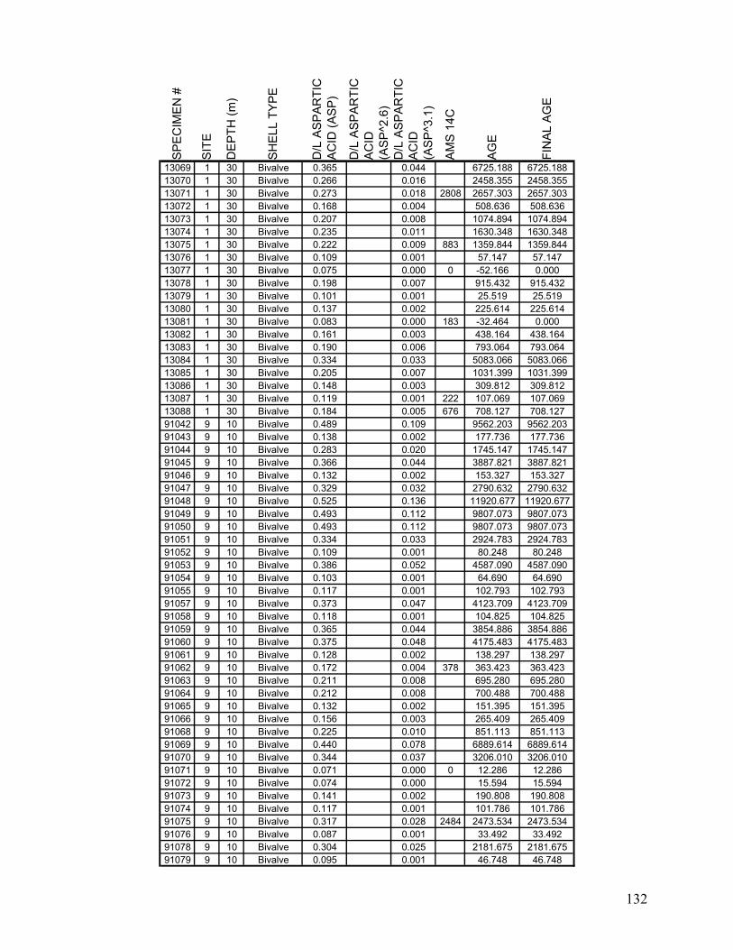
132
SPEC
IMEN
#
SITE
DEP
TH (m
)
SHEL
L TY
PE
D/L
ASP
ARTI
C
ACID
(ASP
)
D/L
ASP
ARTI
C
ACID
(A
SP^2
.6)
D/L
ASP
ARTI
C
ACID
(A
SP^3
.1)
AMS
14C
AGE
FIN
AL A
GE
13069 1 30 Bivalve 0.365 0.044 6725.188 6725.18813070 1 30 Bivalve 0.266 0.016 2458.355 2458.35513071 1 30 Bivalve 0.273 0.018 2808 2657.303 2657.30313072 1 30 Bivalve 0.168 0.004 508.636 508.63613073 1 30 Bivalve 0.207 0.008 1074.894 1074.89413074 1 30 Bivalve 0.235 0.011 1630.348 1630.34813075 1 30 Bivalve 0.222 0.009 883 1359.844 1359.84413076 1 30 Bivalve 0.109 0.001 57.147 57.14713077 1 30 Bivalve 0.075 0.000 0 -52.166 0.00013078 1 30 Bivalve 0.198 0.007 915.432 915.43213079 1 30 Bivalve 0.101 0.001 25.519 25.51913080 1 30 Bivalve 0.137 0.002 225.614 225.61413081 1 30 Bivalve 0.083 0.000 183 -32.464 0.00013082 1 30 Bivalve 0.161 0.003 438.164 438.16413083 1 30 Bivalve 0.190 0.006 793.064 793.06413084 1 30 Bivalve 0.334 0.033 5083.066 5083.06613085 1 30 Bivalve 0.205 0.007 1031.399 1031.39913086 1 30 Bivalve 0.148 0.003 309.812 309.81213087 1 30 Bivalve 0.119 0.001 222 107.069 107.06913088 1 30 Bivalve 0.184 0.005 676 708.127 708.12791042 9 10 Bivalve 0.489 0.109 9562.203 9562.20391043 9 10 Bivalve 0.138 0.002 177.736 177.73691044 9 10 Bivalve 0.283 0.020 1745.147 1745.14791045 9 10 Bivalve 0.366 0.044 3887.821 3887.82191046 9 10 Bivalve 0.132 0.002 153.327 153.32791047 9 10 Bivalve 0.329 0.032 2790.632 2790.63291048 9 10 Bivalve 0.525 0.136 11920.677 11920.67791049 9 10 Bivalve 0.493 0.112 9807.073 9807.07391050 9 10 Bivalve 0.493 0.112 9807.073 9807.07391051 9 10 Bivalve 0.334 0.033 2924.783 2924.78391052 9 10 Bivalve 0.109 0.001 80.248 80.24891053 9 10 Bivalve 0.386 0.052 4587.090 4587.09091054 9 10 Bivalve 0.103 0.001 64.690 64.69091055 9 10 Bivalve 0.117 0.001 102.793 102.79391057 9 10 Bivalve 0.373 0.047 4123.709 4123.70991058 9 10 Bivalve 0.118 0.001 104.825 104.82591059 9 10 Bivalve 0.365 0.044 3854.886 3854.88691060 9 10 Bivalve 0.375 0.048 4175.483 4175.48391061 9 10 Bivalve 0.128 0.002 138.297 138.29791062 9 10 Bivalve 0.172 0.004 378 363.423 363.42391063 9 10 Bivalve 0.211 0.008 695.280 695.28091064 9 10 Bivalve 0.212 0.008 700.488 700.48891065 9 10 Bivalve 0.132 0.002 151.395 151.39591066 9 10 Bivalve 0.156 0.003 265.409 265.40991068 9 10 Bivalve 0.225 0.010 851.113 851.11391069 9 10 Bivalve 0.440 0.078 6889.614 6889.61491070 9 10 Bivalve 0.344 0.037 3206.010 3206.01091071 9 10 Bivalve 0.071 0.000 0 12.286 12.28691072 9 10 Bivalve 0.074 0.000 15.594 15.59491073 9 10 Bivalve 0.141 0.002 190.808 190.80891074 9 10 Bivalve 0.117 0.001 101.786 101.78691075 9 10 Bivalve 0.317 0.028 2484 2473.534 2473.53491076 9 10 Bivalve 0.087 0.001 33.492 33.49291078 9 10 Bivalve 0.304 0.025 2181.675 2181.67591079 9 10 Bivalve 0.095 0.001 46.748 46.748

133
Appendix 3.2: Bootstrap program for SAS/IML This is a balanced bootstrap program for estimating the confidence intervals around the semi-quartile range. The program was written in SAS and SAS/IML (Ver. 9.1) by R. Krause. It is a modified version of a program written by M. Kowalewski (Kowalewski et al., 1998). The program should work in any version of SAS. It requires a data set of raw scores for one variable. The data should be typed or copied into the program where indicated. %let times=5000; * - enter the desired number of iterations; data data1; infile cards; input var1; cards; * - enter data in the space below (between “cards” and the floating semi colon); ; PROC UNIVARIATE data=data1 noprint; var var1; output out=initial n=n std=std pctlpre=p pctlpts=25 75; PROC PRINT data=initial; PROC IML; USE data1; READ ALL INTO X; *** MODULE 'RANVEC' creates a new vector 'v_out' by resampling without replacement the input vector 'in'; START ranvec(in,v_out); k=nrow(in); v_index=in; do i=1 to k; rand=floor((k-i+1)*ranuni(0) + 1); v_ran=v_ran||v_index[rand]; v_index=remove(v_index,rand); end; v_out=v_ran; FINISH ranvec; *** MODULE 'MIXUP' creates a template of row and column ids for balanced-bootstrap resampling; START mixup(X,times,template); n=nrow(X); template=t(1:n)*j(1,times,1); do i=1 to times; run ranvec(template[,i],out); template[,i]=t(out); end; do i=1 to n; run ranvec(t(template[i,]),out); template[i,]=out; end; FINISH mixup; *** MODULE 'RANDOM' invokes other modules and executes a simulation; START random(X,times,out); quar=quartile(X); *calculates actual semiquatile range; q1=quar[2,]; q3=quar[4,]; asqr=(q3-q1)/2; print 'Actual semi-quartile range of sample =' asqr; run mixup(X,times,template);
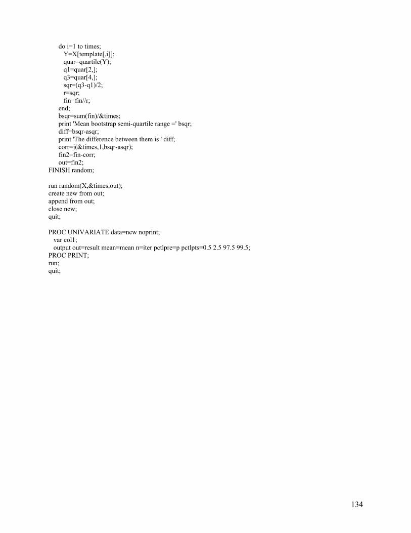
134
do i=1 to times; Y=X[template[,i]]; quar=quartile(Y); q1=quar[2,]; q3=quar[4,]; sqr=(q3-q1)/2; r=sqr; fin=fin//r; end; bsqr=sum(fin)/× print 'Mean bootstrap semi-quartile range =' bsqr; diff=bsqr-asqr; print 'The difference between them is ' diff; corr=j(×,1,bsqr-asqr); fin2=fin-corr; out=fin2; FINISH random; run random(X,×,out); create new from out; append from out; close new; quit; PROC UNIVARIATE data=new noprint; var col1; output out=result mean=mean n=iter pctlpre=p pctlpts=0.5 2.5 97.5 99.5; PROC PRINT; run; quit;
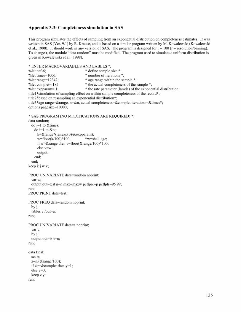
135
Appendix 3.3: Completeness simulation in SAS This program simulates the effects of sampling from an exponential distribution on completeness estimates. It was written in SAS (Ver. 9.1) by R. Krause, and is based on a similar program written by M. Kowalewski (Kowalewski et al., 1998). It should work in any version of SAS. The program is designed for r = 100 (r = resolution/binning). To change r, the module “data random” must be modified. The program used to simulate a uniform distribution is given in Kowalewski et al. (1998). * ENTER MACROVARIABLES AND LABELS *; %let n=36; * define sample size *; %let times=1000; * number of iterations *; %let range=12342; * age range within the sample *; %let complet=.185; * the actual completeness of the sample *; %let expparam=.1; * the rate parameter (lamda) of the exponential distribution; title1*simulation of sampling effect on within-sample completeness of the record*; title2*based on resampling an exponential distribution*; title3*age range=&range, n=&n, actual completeness=&complet iterations=×*; options pagesize=10000; * SAS PROGRAM (NO MODIFICATIONS ARE REQUIRED) *; data random; do j=1 to × do i=1 to &n; k=&range*(ranexp(0)/&expparam); w=floor(k/100)*100; *w=shell age; if w>&range then v=floor(&range/100)*100; else v=w ; output; end; end; keep k j w v; PROC UNIVARIATE data=random noprint; var w; output out=test n=n max=maxw pctlpre=p pctlpts=95 99; run; PROC PRINT data=test; PROC FREQ data=random noprint; by j; tables v /out=a; run; PROC UNIVARIATE data=a noprint; var v; by j; output out=b n=n; run; data final; set b; z=n/(&range/100); if z>=&complet then y=1; else y=0; keep z y; run;
136
PROC PRINT; Title4'the expected sample completeness and its 95 and 99 confidence intervals'; PROC UNIVARIATE data=final noprint; var z; output out=result mean=mean n=iter pctlpre=p pctlpts=0.5 2.5 97.5 99.5; PROC PRINT; run; PROC UNIVARIATE data=final noprint; var y; output out=result2 sum=p; run; Title5'Probability that the original sample came from 100%-complete, exponentially distributed record'; Title6'probA = the probability of greater completeness than actual'; Title7'probB = the probability of lesser completeness than actual'; data prob; set result2; probA=p/× probB=1-probA; PROC PRINT; run; quit;