Embed Size (px)
Citation preview
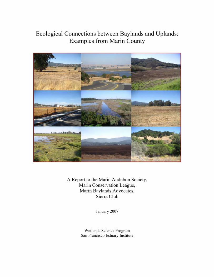
Ecological Connections between Baylands and Uplands: Examples from Marin County
A Report to the Marin Audubon Society, Marin Conservation League, Marin Baylands Advocates,
Sierra Club
January 2007
Wetlands Science Program San Francisco Estuary Institute

Ecological Connections between Baylands and Uplands: Examples from Marin County
Josh Collins, San Francisco Estuary Institute
Joe Didonato, East Bay Regional Park District
Geoff Geupel, PRBO Conservation Science
Letitia Grenier, San Francisco Estuary Institute
Tom Kucera, Kucera Consulting
Bill Lidicker, University of California Berkeley
Bill Rainey, University of California Berkeley
Steve Rottenborn, H.T. Harvey and Associates
Historical Ecology: Robin Grossinger and Elise Brewster, SFEI
Geographic Information System: Kristen Larned and Micha Salomon, SFEI
January 2007
SFEI Report No. 521

Table of Contents
Executive Summary..............................................................................................1
Purpose .............................................................................................................3
Relevance .............................................................................................................3
Methods and Results.............................................................................................5
Key Terms.................................................................................................5
Assumptions..............................................................................................5
Landscape Maps........................................................................................6
Physiography.............................................................................................9
Focal Species Selection...........................................................................10
Salt marsh harvest mouse (Reithrodontomys raviventris) .............12
California ground squirrel (Spermophilus beecheyi) .....................13
California meadow vole (Microtus californicus)...........................14
Pallid bat (Antrozous pallidus).......................................................15
Yuma bat (Myotis yumanensis)......................................................16
Song sparrow (Melospiza melodia) ...............................................17
Great blue heron and great egret (Ardea herodias and A. alba) ....18
Northern harrier (Circus cyaneus) .................................................19
Tree swallow (Tachycineta bicolor) ..............................................20
Migratory shorebirds......................................................................21
Coyote (Canis latrans)...................................................................22
Discussion ........................................................................................................23
Recommendations...............................................................................................24
Citations ........................................................................................................27
Appendix A: Definitions of Key Terms..............................................................35
Appendix B: Science Team Biographies ............................................................37
Appendix C: Science Workshop Agenda ...........................................................39
Appendix D: GIS Rules and Maps of Focal Species Distributions ……………41

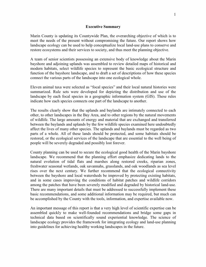
1
Executive Summary
Marin County is updating its Countywide Plan, the overarching objective of which is to meet the needs of the present without compromising the future. Our report shows how landscape ecology can be used to help conceptualize local land-use plans to conserve and restore ecosystems and their services to society, and thus meet the planning objective. A team of senior scientists possessing an extensive body of knowledge about the Marin bayshore and adjoining uplands was assembled to review detailed maps of historical and modern habitats, select wildlife species to represent the basic ecological structure and function of the bayshore landscape, and to draft a set of descriptions of how these species connect the various parts of the landscape into one ecological whole. Eleven animal taxa were selected as “focal species” and their local natural histories were summarized. Rule sets were developed for depicting the distribution and use of the landscape by each focal species in a geographic information system (GIS). These rules indicate how each species connects one part of the landscape to another. The results clearly show that the uplands and baylands are intimately connected to each other, to other landscapes in the Bay Area, and to other regions by the natural movements of wildlife. The large amounts of energy and material that are exchanged and transferred between the baylands and uplands by the few wildlife species examined here undoubtedly affect the lives of many other species. The uplands and baylands must be regarded as two parts of a whole. All of these lands should be protected, and some habitats should be restored, or the ecological services of the landscape that are essential to the well being of people will be severely degraded and possibly lost forever. County planning can be used to secure the ecological good health of the Marin bayshore landscape. We recommend that the planning effort emphasize dedicating lands to the natural evolution of tidal flats and marshes along restored creeks, riparian zones, freshwater seasonal wetlands, oak savannahs, grasslands, and oak woodlands as sea level rises over the next century. We further recommend that the ecological connectivity between the bayshore and local watersheds be improved by protecting existing habitats, and in some cases improving the conditions of habitat patches and wildlife corridors among the patches that have been severely modified and degraded by historical land-use. There are many important details that must be addressed to successfully implement these basic recommendations, and some additional information may be required, but much can be accomplished by the County with the tools, information, and expertise available now. An important message of this report is that a very high level of scientific expertise can be assembled quickly to make well-founded recommendations and bridge some gaps in technical data based on scientifically sound experiential knowledge. The science of landscape ecology provides the framework for integrating ecology and land-use planning into guidelines for achieving healthy working landscapes in the future.

2
3
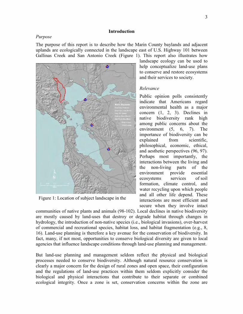
Introduction Purpose The purpose of this report is to describe how the Marin County baylands and adjacent uplands are ecologically connected in the landscape east of U.S. Highway 101 between Gallinas Creek and San Antonio Creek (Figure 1). This report also illustrates how
landscape ecology can be used to help conceptualize land-use plans to conserve and restore ecosystems and their services to society. Relevance Public opinion polls consistently indicate that Americans regard environmental health as a major concern (1, 2, 3). Declines in native biodiversity rank high among public concerns about the environment (5, 6, 7). The importance of biodiversity can be explained from scientific, philosophical, economic, ethical, and aesthetic perspectives (96, 97). Perhaps most importantly, the interactions between the living and the non-living parts of the environment provide essential ecosystems services of soil formation, climate control, and water recycling upon which people and all other life depend. These interactions are most efficient and secure when they involve intact
communities of native plants and animals (98-102). Local declines in native biodiversity are mostly caused by land-uses that destroy or degrade habitat through changes in hydrology, the introduction of non-native species (i.e., biological invasions), over-harvest of commercial and recreational species, habitat loss, and habitat fragmentation (e.g., 8, 16). Land-use planning is therefore a key avenue for the conservation of biodiversity. In fact, many, if not most, opportunities to conserve biological diversity are given to local agencies that influence landscape conditions through land-use planning and management. But land-use planning and management seldom reflect the physical and biological processes needed to conserve biodiversity. Although natural resource conservation is clearly a major concern for the design of rural zones and open space, their configuration and the regulations of land-use practices within them seldom explicitly consider the biological and physical interactions that contribute to their separate or combined ecological integrity. Once a zone is set, conservation concerns within the zone are
Figure 1: Location of subject landscape in the B A
4
addressed piecemeal through individual land-use changes, without a framework for considering their cumulative ecological effects. Unless the land-use zones reflect the spatial organization of ecosystems, and unless the decisions about land-uses within the zones are guided by a plan for overall biodiversity conservation, the natural processes that support biodiversity will tend to degrade\ and the objectives to sustain biodiversity will not be met. Empirical evidence indicates that when land-use planning is not adequately guided by the specific needs of multiple species that together represent a naturalistic ecological complexity at the landscape scale, patches of habitat get smaller and more distant from each other, with unnatural amounts of edge per unit area and less connectivity overall, which in turn increases the rates of biological invasion, local extinction, and overall declines in native biodiversity (16). Marin County is preparing an Environmental Impact Report (EIR) for the Countywide Plan Update. Meeting the needs of the present without compromising the future is the overarching theme. To help assure that the plan is consistent with this theme, the County has developed a set of ten guiding principles, the first and fourth of which relate directly to biodiversity and to the environment more generally (18):
1. Link equity, economy, and the environment locally, regionally and globally: we will improve the vitality of our community, economy, and environment. We will seek innovations that provide multiple benefits to Marin County. Examples of Community Indicators include GPI (Genuine Progress Indicator: comprehensive, aggregate measure of general well being and sustainability including economic, social and ecological costs);
2. Steward our natural and agricultural assets: we will continue to protect open space and wilderness, and enhance habitats and bio-diversity; we will protect and support agricultural lands and activities and provide markets for fresh, locally grown food (examples of Community Indicators include acres of wilderness; acres of protected land; level of fish populations; track special status plants and animals; quantity of topsoil; active farmland by crop; productivity of acreage and crop value of agricultural land; acres of organic farmland).
The Countywide Plan will have to be implemented and enforced on a case-by case basis, one land-use decision at a time. And yet the plan strives to protect attributes of the environment, such as the conservation of biodiversity and environmental vitality that can only be protected through a coordinated effort among multiple cases and decisions. Land-use zones and policies can be the right avenues for this coordination if they are consistent with the overarching conservation efforts. This brief report illustrates how basic principles of ecosystem science landscape ecology might be practically applied by local land-use planners and managers to improve the security and vitality of our human community, economy, and environment by conserving and enhancing ecological connections locally, regionally, and globally.
5
Methods and Results Key Terms This report is easier to understand given the definitions of key technical terms provided in Appendix A. Perhaps the most important of these terms are “biodiversity,” and “ecological connectivity.” Biodiversity means the variability among all living organisms from all kinds of environments within a landscape. It includes the diversity within species, between species, and of ecosystems (8). Ecological connectivity, also termed “connectivity between habitats,” is a measure of the ability of organisms to move among patches of habitat (16).
Assumptions This report makes the following basic assumptions.
• The ability of ecosystems to provide their essential services depends on natural levels of native biodiversity to maintain food-chain length, food-web complexity, and ecological redundancy which, in turn, maintains ecosystem resistance and resilience to stress and disturbance (7, 8).
• Wildlife movements within and between patches, corridors, and other landscape elements need to be understood well enough to support management actions that sustain native biodiversity (16).
• Natural landscapes encompass a suite of climatic, geologic, and ecologic processes, such as fire, flooding, and plant community succession, that tend to reproduce or sustain a particular composition and arrangement of landscape elements. Well managed, working landscapes provide the key ecological services of natural landscapes while also supporting people. Land-use planning plays a prominent role in determining the form and function of working landscapes.
• Landscapes don’t work well when land-use and natural processes are in conflict. Meeting the needs of people and wildlife takes quantities of space and time that are only available on large spatial and temporal scales.
• People and wildlife must coexist. Healthy coexistence can be achieved through landscape planning. Ecological services can be restored to landscapes through their careful design and maintenance.
• The optimal landscape configuration may not be known, but historical conditions (i.e., the form of landscapes prior to Euroamerican contact) indicate the patch composition and arrangement that tends to naturally occur, given the local template of geology and climate. While planners cannot “reach the past,” the historical landscape provides clues about achievable, alternative future landscapes (35).
• Corridors that connect relatively large patches along environmental gradients are essential aspects of landscape planning for biodiversity conservation. The gradients are important for sustaining genetic diversity that enables species to accommodate environmental change.
6
• The habitat needs of focal species can be used as design criteria for working landscapes. In other words, the optimal composition and arrangement of landscape elements to sustain focal species will yield adequate levels of most of the endemic ecological services.
• The ultimate goal of conservation biology is to permit the natural persistence and evolution of species. Landscapes need to support native plants and animals through evolutionary time. This means that landscapes need to sustain adequate ecological connectivity among key habitat patches arrayed along gradients of environmental processes.
Landscape Maps Base maps were produced of the historical landscape (i.e., pre-Euroamerican contact) and current landscape (folded Figures 2 and 3). The maps depict (as patches) all surface water features (i.e., tidal and fluvial creeks, wetlands, tidal flats, lakes, etc), major terrestrial plant communities, and developed land cover types. The classification of water features is based on the National Wetlands Inventory (NWI) of the USFWS (22), which we updated for the subject landscape. The NWI updates were based on the “1m resolution” NAIP imagery (21) dated 2005. For this imagery, a 1m ground sample distance (GSD) is within 5m of a reference ortho image. The draft NWI updates were verified with field visits. The wetland patch names on the updated NWI map were then translated into the regional nomenclature for wetlands and riparian areas according to the crosswalk provided by the California Rapid Assessment Method (23). The classification of developed land cover types is based on the National Land Cover System of the USGS (24). The classification of plant communities is derived from the CalVeg maps (19) and California Vegetation Manual (25, 26). Ancillary sources of information about the locations of wetlands included local environmental impact reports, site plans, and visits to the field. The historical landscape mapping was based on the earliest available aerial photography, 19th-century maps and surveys, and existing landscape patterns (as evidenced in contemporary aerial photography, previous environmental assessments, and fieldwork). Aerial imagery from the years 1930, 1942, 1946, and 1952 was acquired from the UC Berkeley Earth Sciences and Map Library and the Southern Sonoma Resource Conservation District. The distribution of terrestrial vegetation communities was derived from modern imagery depicting remnant community patches, early aerial photography, and the historical topographic maps (termed “T-sheets) of the United States Coast Survey/Coast and Geodetic Survey (33, 27). Since these data sets did not entirely cover the subject landscape, some amount of extrapolation based on aspect, elevation, and soils was required. A number of historical vegetation features were identified that are no longer present. A preliminary assessment was made of major historical changes in terrestrial vegetation patterns, including loss/fragmentation of forest and woodland and, in some places, increased stand density. However, this was not a full assessment of trends in terrestrial vegetation communities, which would involve more assessment of early wood cutting/timber harvest and quantification of woodlands/scrub expansion in the second half of the 20th century.
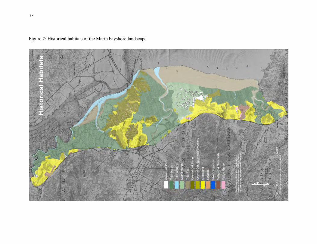
7Figure 2: Historical habitats of the Marin bayshore landscape
8
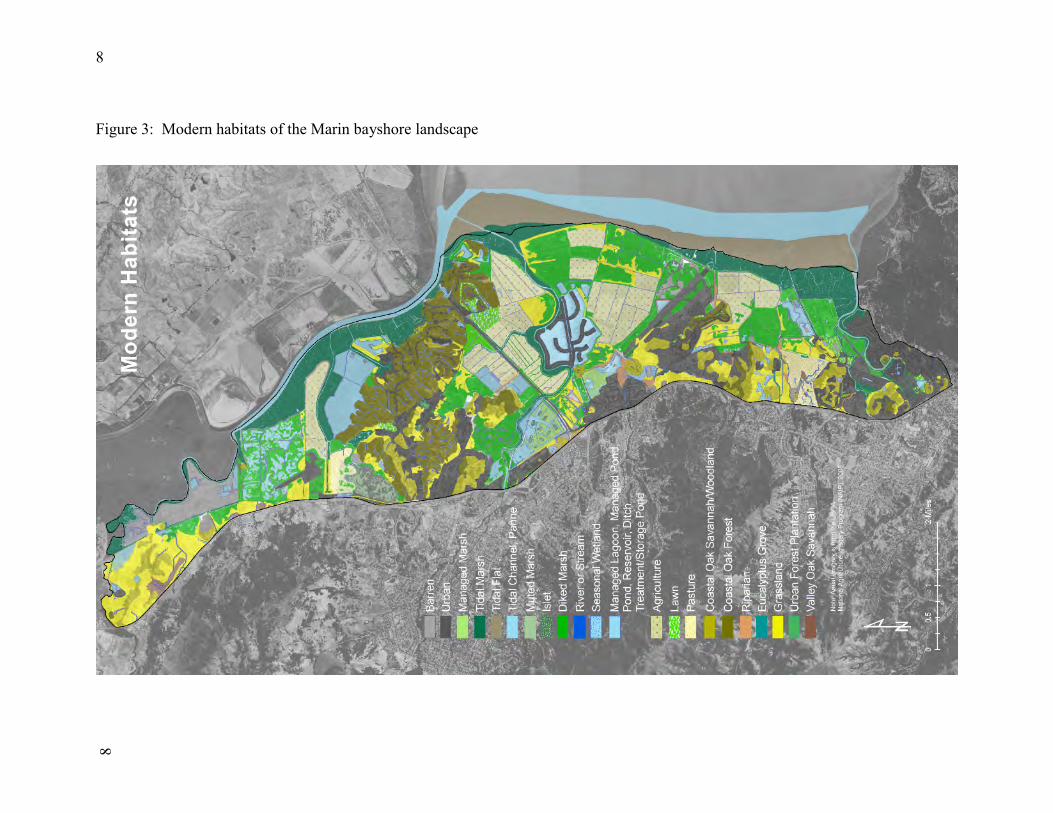
8Figure 3: Modern habitats of the Marin bayshore landscape
9
Savanna and grasslands are differentiated by the density of their trees (i.e., the number of trees per unit area of landscape). We defined valley oak savanna as having a minimum of 1-2 trees per acre (determined from historical oak savanna mapping in the Napa and Santa Clara valleys) in the characteristic pattern on low-elevation alluvial plains. Oak savanna in the northern portion of the study area was identified primarily using early aerial photography. The T-sheets provided evidence farther south. The USCGS (27) explicitly showed a large savanna adjoining the lower reaches of Miller Creek. The early T-sheet (33) erroneously shows nearly continuous forest along the Marin shoreline. This map was surveyed by Rodgers, whose tended to show less detail than other surveyors of the USCS (28, 29). For example, he shows trees covering the valley north from Pacheco Hill, whereas Loring (31), who crossed this area, shows no trees here. Early aerial photography also shows no trees. Miller Creek, Arroyo San Jose, and the creek flowing north from Pacheco Hill along Highway 101 appear to have not reached the tidal margin in well-defined channels prior to modification by European settlers (27, 33, 34). Early T-sheets show adjacent tidal channel networks terminating in small "dead-end" sloughs, and not connecting to the creeks. Present-day creek "extensions" into the baylands are obviously man-made. The lack of natural channels connecting these creeks to tidal marsh does not mean that creek flows never reached the bay. Matthewson (32), in his General Land Office survey, noted that the "confluence of Arroyo San Jose with the salt marsh" was 15 links (~10 feet) wide. However, near Burdell, Matthewson referred to a tidal slough as an “arroyo,” which suggests he wasn’t always clear about distinguishing fluvial channels from tidal channels. The actual confluence with Arroyo San Jose may have been a swale or shallow channel that was mapped by some surveyors and not others. It’s likely that flow from these creeks reached the adjacent tidal marsh during especially wet years and during major rainstorms, even if the flow was not conveyed by a well-defined channel. Several dense groves of trees willow trees are evident in the T-sheets at the downstream end of terminal streams, near the edge of tidal marsh. Some groves still exist close to their original locations near the historical termini of Miller Creek and Arroyo San Jose. Physiography The basic physiography of the landscape is determined by geology and climate. It has changed little since the Bay achieved its approximate current extent 2-3 thousand year ago. The average annual amount of rainfall still varies around 27 inches, with most rain falling between November and March. Air temperatures remain mild year-round. The local watersheds mostly consist of highly erodable sandstones, sheared shales, metavolcanic rock, serpentine, and various conglomerates (90). They continue to be uplifted, and they erode easily into narrow valleys along steep tributary streams that come together as slightly broader valleys draining to the Bay. These are all that remain of valleys being drowned by the Bay as it rises. The result is a landscape of tidal flats and marshes fronting little valleys among rolling hills of moderate height and steepness. Some of the hilltops have become islands surrounded by baylands due to the Bay rising. The geologic and climatic processes that account for the basic structure and form of the
10
landscape are ongoing and essentially unmanageable, except to the extent that we can accommodate them through landscape design and land-use planning. People have locally modified the physiography of the landscape by moving and channelizing streams, reclaiming tidal flats and marshlands, grading hilltops and valleys for military, residential, and commercial development, and by constructing roadways, These modifications have changed the distribution and abundance of habitats and the connections between them more than any natural forces and processes, While the basic physiography of the landscape has not historically changed, the number and kinds and amount of ecological services have changed, mainly due to land use. Focal Species Selection Planning for the protection of ecosystems and landscapes requires a broad range of environmental and social expertise. Here we focus on the wildlife conservation aspects only. This is a complex undertaking requiring much knowledge about a great variety of wildlife species. Our approach was to assemble a team of senior experts who are familiar with conservation planning, the particular landscape of interest, a variety of wildlife species endemic to the landscape, and the scientific literature pertaining to these topics. Recruiting team members was not difficult. The Bay Area is rich with ecological and conservation expertise. The short biographies of the participating scientists are included as Appendix B. Together the team members represent nearly 200 years of professional experience as research ecologists and practitioners of conservation biology. Each team member also represents a network of other scientists with whom technical matters pertaining to this project could be discussed at will. The science team met for a full day to select focal species and describe how they connect the baylands and uplands of the subject landscape. The agenda for that one day workshop is included as Appendix C. The team agreed to focus on the bayland-upland connectivity because this topic is most relevant to Marin County’s planning process. The selection of focal species was based on the team’s collective understanding of the species’ natural histories – their habitat needs, feeding behavior, diets, and patterns of dispersal and migration. No new data about the focal species were collected for this report. Once the focal species were selected, the science team developed rules for depicting their distribution on the base maps. The results were summarized as conceptual models of specific connections between landscape elements. Maps of the expected historical and current distribution of the focal species are presented in Appendix D. The science team selected focal species to represent a variety of ways in which the uplands and baylands are ecologically connected within the subject landscape, and how this landscape is connected to the rest of the region and beyond (Table 1). Many additional species could also be examined in the same manner. The species selected are useful for the reasons given, but they are best thought of as examples of a large suite of focal species that might be considered during a more comprehensive landscape analysis or planning effort. The species selected are ubiquitous within one or more dominant
11
elements of the subject landscape, and therefore illustrate some of the most pervasive ecological connectivity among habitat types. They are not, however, especially well connected to each other. For example they do not all belong to the same clearly defined food web. In fact, they represent a variety of different food webs that are certainly connected, but not always through the selected focal species.
Table 1: List of focal species and their rationale for selection.
Focal Species Rationale for Selection
salt marsh harvest mouse
1. Endangered species that connects baylands to fringing uplands used as refuge from flooding.
2. Food resource for predators that move between uplands and baylands. 3. Demonstrates need for contiguous habitat along major environmental gradients.
California ground squirrel
1. Daily foraging connects grasslands to tidal and diked baylands. 2. Keystone species through burrow construction in grasslands and savannas. 3. Abundant in working landscapes and easily observed by the public.
California meadow vole
1. Seasonal migration and foraging connects tidal baylands to grasslands. 2. Abundant food resource for predators including those that move between uplands
and baylands. 3. Demonstrates the need for migration corridors.
pallid bat 1. Foraging connects woodlands and urban areas to grasslands and diked baylands. 2. Demonstrates nocturnal ecological connectivity. 3. Can be abundant in working landscapes.
Yuma bat 1. Foraging connects woodlands and urban areas to wetlands and aquatic patches. 2. Significant predator on nuisance insects including mosquitoes. 3. Responds especially well to population conservation efforts.
song sparrows
1. Foraging and refuge from flooding connect tidal baylands to riparian areas. 2. Demonstrates need for contiguous habitat patches along environmental gradients. 3. Abundant in working landscapes and is easily observed by the public.
great blue heron and great egret
1. Foraging as top predators connects grassland and fringing woodland to baylands. 2. Demonstrates connectivity to other landscapes within the region. 3. Common and are easily observed by the public.
northern harrier
1. Foraging connects grasslands and savannas to tidal and diked baylands. 2. Top predator for the baylands. 3. Common in working landscapes and easily observed by the public.
tree swallow 1. Foraging connects woodlands and riparian areas to diked and tidal baylands. 2. Significant predator on nuisance insects including mosquitoes. 3. Responds especially well to population conservation efforts.
migratory shorebirds
1. Foraging connects seasonal wetlands and grasslands to tidal and diked baylands. 2. Demonstrate connectivity to other landscapes beyond region. 3. Abundant in working landscapes and easily observed by the public.
coyote 1. Foraging connects all uplands to all baylands. 2. Keystone species through regulation of other predator populations. 3. Demonstrates connectivity to adjacent landscapes.
12
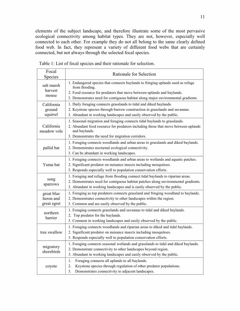
Salt marsh harvest mouse (Reithrodontomys raviventris)
The salt marsh harvest mouse is an endangered tidal marsh endemic (93) that illustrates the importance of the upland-tidal marsh transition zone (94), and the importance of connecting habitat patches along environmental gradients (95). These mice are small, relatively slow-moving, nocturnal rodents endemic to saline and brackish tidal marshes of San Francisco Bay (42, 45, 40, 36, 37). They also inhabit diked baylands that support dense salt marsh vegetation (44, 46, 92). When the marsh vegetation is flooded, the mice seek refuge in dense vegetation in the upland-tidal marsh boundary that
conceals them from their predators (44, 45). After flood waters recede, the surviving mice return to the marshland. A zone of vegetation along the marsh flood line is therefore important for the survival of salt marsh harvest mice (40, 45). The fact that these mice inhabit tidal marshes across a range of salinity conditions may be important (95). Their exposure to varying salinity regimes can help maintain their ability to survive the natural seasonal and inter-annual variability in salinity. Restricting the mice to one salinity regime could eventually eliminate this flexibility. The population of salt marsh harvest mice therefore benefits from having access among patches of tidal marsh that span the salinity gradient. Such an arrangement of patches can be provided by fringing marsh along the salinity gradient of local creeks, and by bayshore marshes that span the main estuarine gradient of the Bay. The habitat along local creeks tends to consist of small patches, however, that provide less protection than do the larger patches that usually form along the bayshore. Salt marsh harvest mice historically had very large patches of tidal marshland arrayed along the bayshore and along local creeks. Suitable upland refuge adjoined this preferred habitat (Appendix D, Figure D1). Although the amount of tidal marsh has been greatly decreased, large patches still exist along the bayshore between the local creeks (Appendix D, Figure D2) with corridors of narrow tidal marsh and diked marsh connecting the larger tidal marsh patches. But the tidal marshland along the creeks mostly consists of thin corridors and patches with narrow buffers adjoining developed land that offers little protection from outside disturbance and stress. Much of the upland refuge consists of sparsely vegetated earthen levees that serve as corridors for many predators of salt marsh harvest mice.
Figure 4: Conceptual model of connectivity provided by salt marsh harvest mice. The natural habitat is tidal marsh (dark green) but the mice also inhabit diked marsh (light-green), and require upland refuge (olive-green). They should be able to disperse easily among habitat patches arrayed along the salinity gradients of local creeks, and these small patches should be connected to larger, adjacent or nearby patches along the bayshore. Levees are important as refuge but they also provide access for predators.
SF State University
Across Diked Marsh
Upland Matrix
Tidal Marsh Along Bayshore
Alo
ngC
reek
Alo
ngC
reek
13
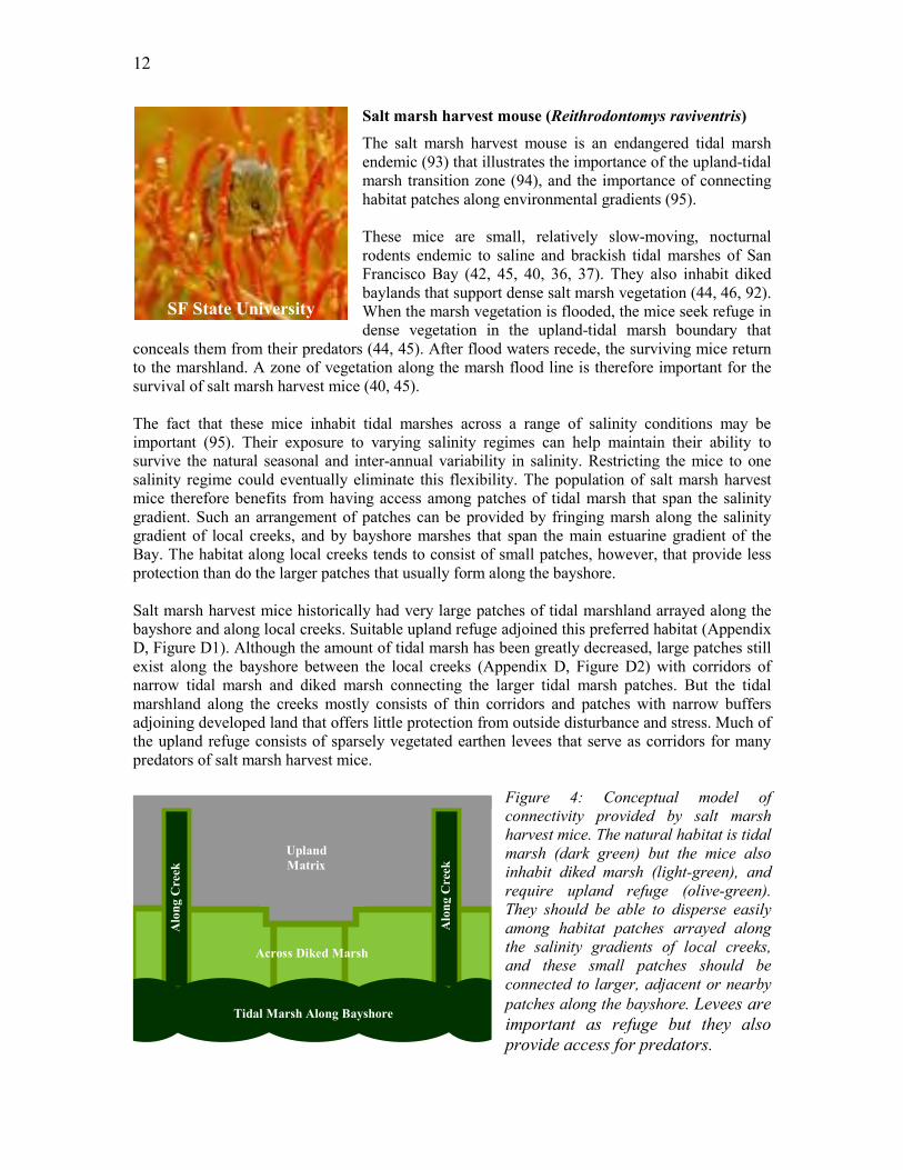
California ground squirrel (Spermophilus beecheyi) The California ground squirrel was selected because of its close association with diked baylands and the upland-tidal marsh boundary, and because many wildlife species benefit from the presence of healthy populations of ground squirrels. Ground squirrels colonize the margins of grassy hills and levees. Extensive burrow systems can support many individuals for multiple generations (47). Ground squirrels spend long periods each day above ground feeding on green
vegetation, seeds, roots, mushrooms, and insects. But they rarely venture more than about 150m from their burrows (48, 49). They are mainly a grassland species, but they also enter adjacent baylands to feed. Ground squirrels are ecological engineers (50, 51), meaning that they provide habitat for many other species. They’re especially important for species that spend time below ground but cannot excavate their own burrows. Many native predators, including hawks, coyotes, golden eagles, northern Pacific rattlesnakes, and gopher snakes are closely associated with ground squirrel colonies. The historical landscape featured abundant transition zones between grassy hillsides colonized by ground squirrels and patches of grasslands, oak savanna, and high tidal marsh that offered food resources (Appendix D, Figure D3). Most of this natural upland edge has been replaced by levees and road grades that ground squirrels readily colonize. The high tidal marsh, grasslands and oak savanna have been largely replaced by diked marsh and pasture that provide some food resources and adjoin inhabitable levees (Appendix D, Figure D4). Although the amount of natural transition zones between hillsides and foraging areas has been reduced, the remaining patches are large enough and close enough to burrow habitat to support abundant ground squirrels. Major creeks and roadways, such as Novato Creek, Black John Slough, and Highway 37 represent significant dispersal barriers. But the vegetated levees can function as inhabitable corridors linking adequate patches of foraging habitat between these barriers.
Figure 5: Conceptual model of connectivity provided by California ground squirrels. The ground squirrels colonize the levees, road grades, and upland margins (dark green) but forage in the adjoining transition zone into diked marsh, tidal marsh, pasture, and other grasslands (light-
green). They do not usually use riparian areas. The gray area represents the interior reaches of patches that are too far from the colonies to be used for foraging and are too sparsely vegetated to serve as dispersal corridors. The network of levees, roadways, and hillsides functions as a template of colony sites and adjacent foraging areas. This pattern is replicated between major barriers to dispersal, such as Novato Creek, Highway 37, and Black John Slough.
UC Davis
Tidal Marsh Matrix
Miscel.Matrix
Miscel.Matrix
Diked Matrix
Diked Matrix
Diked Matrix
Cre
ekM
atri
x
Cre
ekM
atri
x
Upland Matrix
Cre
ekm
atri
x
Upland Matrix
Woodland Matrix
14
California meadow vole (Microtus californicus)
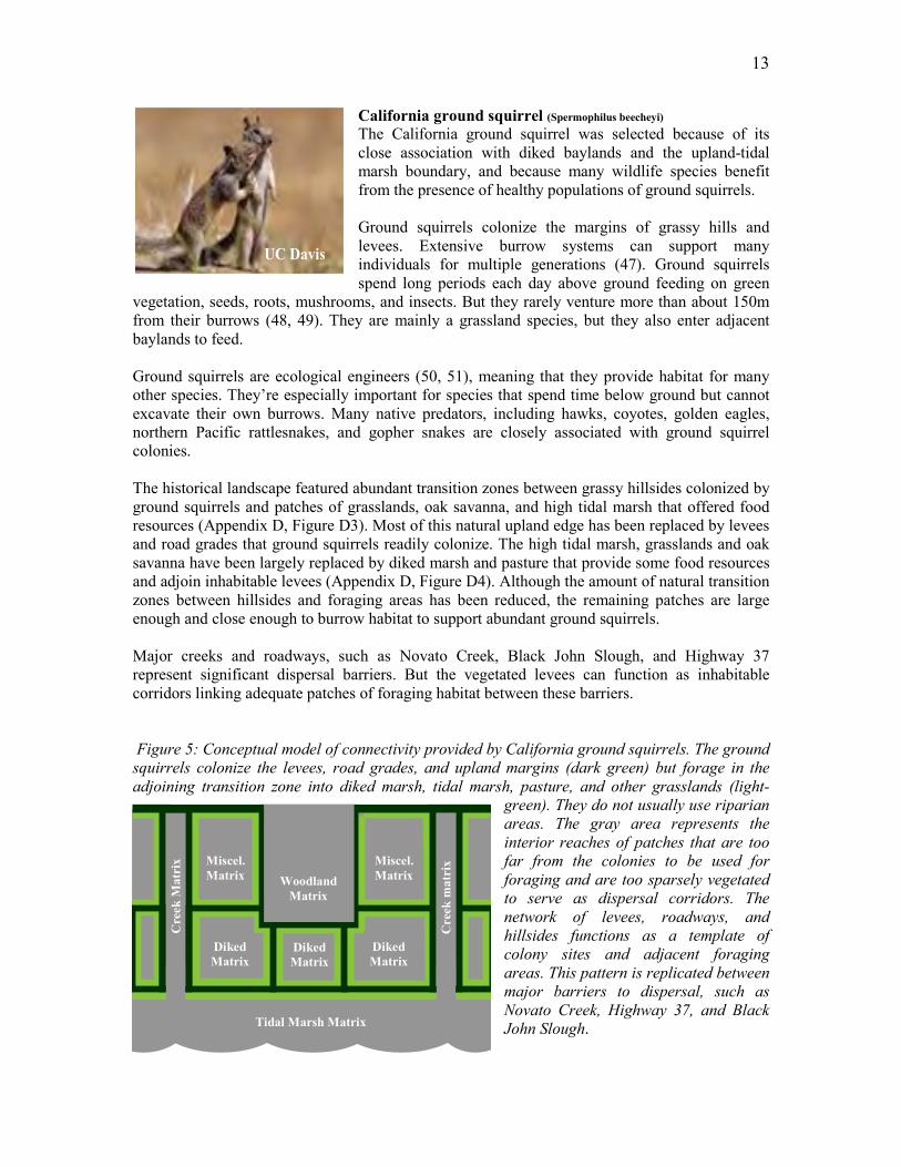
California meadow voles are small, social herbivores that mostly feed on green foliage and roots of living grasses, sedges, and forbs. They can become extremely abundant during years of ample food and reduced predation. Population densities can reach hundreds of voles per acre. The voles forage preferentially around dawn and dusk each
day, with short bursts of activity every few hours in between. In summer they are more nocturnal, and in winter more diurnal. They construct narrow runways and tunnels on the ground surface beneath dense herbaceous vegetation, grasses and surface objects such as boards and logs (52, 54). These runways also serve as the movement paths for other grassland inhabitants. California voles can dominate the diets of many native, ground-dwelling and avian predators. Their high rates of reproduction compensate for the high rates of predation by coyotes, harriers, kites, hawks, owls, herons, egrets, snakes, fox, and feral cats. The voles are known to move seasonally from uplands to tidal marsh (55). During the dry season, as the upland grasses and forbs senesce, voles migrate to wetlands, including tidal marsh, where suitable forage remains. In winter, the voles can migrate back to the uplands to forage on new terrestrial plant growth. Their predators can track the voles’ migration between the baylands and the uplands (74, 91). Some voles use fringing uplands as refuge from flood waters (53). The historical landscape offered abundant high-elevation tidal marshland in large patches for dry season foraging, and broad adjoining areas of upland habitats for foraging during the wet season (Appendix D, Figure D5). The local vole populations must have been very large at times, and their seasonal migrations must have triggered waves of predation. These migrations would account for very large transfers of energy and material between the uplands and baylands throughout the subject landscape. Voles are still vital to the bayshore landscape. But their populations have been reduced by habitat destruction and fragmentation. The grasslands and oak savanna have been replaced by pasture with much less plant cover. The oak woodlands are partly developed and generally separated from the tidal marshlands by large patches of diked marsh and hayfields, most of which do not support suitable plant cover for voles. The seasonal migrations must follow relatively narrow corridors of dense, low-growing vegetation along ditches and levees (Appendix D, Figure D6).
Figure 6: Conceptual model of connectivity provided by California meadow voles. The voles occupy the outer portions of the uplands and diked baylands during the wet season (light green areas) and some migrate to the tidal marsh during the dry season (dark green areas). The matrix (gray areas) consists of interior reaches of these patches that are too sparsely vegetated to usually serve as vole habitat.
UC Santa Barbara
Grassland Matrix
Grassland Matrix
Cre
ekSi
deT
idal
Mar
sh
Diked Marsh Matrix
Diked Marsh Matrix
Diked Marsh Matrix
Woodland Matrix
Cre
ekSi
deT
idal
Mar
sh
Tidal Marsh Along Bayshore
15
Pallid bat (Antrozous pallidus)
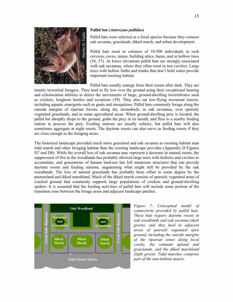
Pallid bats were selected as a focal species because they connect oak savanna, grasslands, diked marsh, and urban development. Pallid bats roost in colonies of 10-500 individuals in rock crevices, caves, mines, building attics, barns, and in hollow trees (56, 57). At lower elevations pallid bats are strongly associated with oak savannas, where they often roost in tree cavities. Large trees with hollow limbs and trunks that don’t hold water provide important roosting habitat. Pallid bats usually emerge from their roosts after dark. They are
mainly terrestrial foragers. They tend to fly low over the ground using their exceptional hearing and echolocation abilities to detect the movements of large, ground-dwelling invertebrates such as crickets, longhorn beetles and scorpions (59). They also eat low-flying nocturnal insects, including aquatic emergents such as gnats and mosquitoes. Pallid bats commonly forage along the outside margins of riparian forests, along dry streambeds, in oak savannas, over sparsely vegetated grasslands, and in some agricultural areas. When ground-dwelling prey is located, the pallid bat abruptly drops to the ground, grabs the prey in its mouth, and flies to a nearby feeding station to process the prey. Feeding stations are usually solitary, but pallid bats will also sometimes aggregate at night roosts. The daytime roosts can also serve as feeding roosts if they are close enough to the foraging areas. The historical landscape provided much more grassland and oak savanna as roosting habitat near tidal marsh and other foraging habitat than the existing landscape provides (Appendix D Figures D7 and D8). While the overall loss of oak savanna may represent a decrease in natural roosts, the suppression of fire in the woodlands has probably allowed large trees with hollows and cavities to accumulate, and generations of human land-use has left numerous structures that can provide daytime roosts and feeding stations, augmenting what might still be provided by the oak woodlands. The loss of natural grasslands has probably been offset to some degree by the pastureland and diked marshland. Much of the diked marsh consists of sparsely vegetated areas of cracked ground that commonly supports large populations of crickets and ground-dwelling spiders. It is assumed that the feeding activities of pallid bats will include some portion of the transition zone between the forage areas and adjacent landscape patches.
Figure 7: Conceptual model of connectivity provided by pallid bats. These bats require daytime roosts in oak woodlands and oak savanna (dark green), and they feed in adjacent areas of sparsely vegetated open ground, including the outside margins of the riparian zones along local creeks, the remnant upland and grasslands, and the diked marshland (light green). Tidal marshes comprise part of the non-habitat matrix.
Mer
linD
.Tut
tle
Oak Woodland
Savanna and
Grassland
Savanna and
Grassland
Cre
ekSi
deR
ipar
ian
Cre
ekSi
deR
ipar
ian
Diked Marsh
Diked Marsh
Diked Marsh
Tidal Marsh Matrix
16
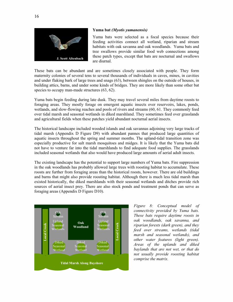
Yuma bat (Myotis yumanensis) Yuma bats were selected as a focal species because their feeding activities connect all wetland, riparian and stream habitats with oak savanna and oak woodlands. Yuma bats and tree swallows provide similar food web connections among these patch types, except that bats are nocturnal and swallows are diurnal.
These bats can be abundant and are sometimes closely associated with people. They form maternity colonies of several tens to several thousands of individuals in caves, mines, in cavities and under flaking bark of large trees and snags (63), between shingles on the outside of houses, in building attics, barns, and under some kinds of bridges. They are more likely than some other bat species to occupy man-made structures (63, 62). Yuma bats begin feeding during late dusk. They may travel several miles from daytime roosts to foraging areas. They mostly forage on emergent aquatic insects over reservoirs, lakes, ponds, wetlands, and slow-flowing reaches and pools of rivers and streams (60, 61. They commonly feed over tidal marsh and seasonal wetlands in diked marshland. They sometimes feed over grasslands and agricultural fields when these patches yield abundant nocturnal aerial insects. The historical landscape included wooded islands and oak savannas adjoining very large tracks of tidal marsh (Appendix D Figure D9) with abundant pannes that produced large quantities of aquatic insects throughout the spring and summer months. The upland-tidal transition zone was especially productive for salt marsh mosquitoes and midges. It is likely that the Yuma bats did not have to venture far into the tidal marshlands to find adequate food supplies. The grasslands included seasonal wetlands that also would have produced large amounts of aerial adult insects. The existing landscape has the potential to support large numbers of Yuma bats. Fire suppression in the oak woodlands has probably allowed large trees with roosting habitat to accumulate. These roosts are further from foraging areas than the historical roosts, however. There are old buildings and barns that might also provide roosting habitat. Although there is much less tidal marsh than existed historically, the diked marshlands with their seasonal wetlands and ditches provide rich sources of aerial insect prey. There are also stock ponds and treatment ponds that can serve as foraging areas (Appendix D Figure D10).
Figure 8: Conceptual model of connectivity provided by Yuma bats. These bats require daytime roosts in oak woodlands, oak savanna, and riparian forests (dark green), and they feed over streams, wetlands (tidal marsh and seasonal wetlands), and other water features (light green). Areas of the uplands and diked baylands that are not wet, or that do not usually provide roosting habitat comprise the matrix.
J. Scott Altenbach
Oak Woodland
Tidal Marsh Along Bayshore
Loc
alC
reek
Loc
alC
reek
Upland Seasonal Wetlands
Upland Seasonal Wetlands
Diked Seasonal Wetland
Diked Seasonal Wetland
Diked Seasonal Wetland
Oak Savann
Oak Savann

17
Song sparrow (Melospiza melodia) Song sparrows are generally territorial in the mid-canopy of trees and tall shrubbery bordering lakes, streams, and wetlands. The San Pablo song sparrow is one of three subspecies that reside in tidal marshland in the Bay Area (38, 39). They prefer high saline tidal marsh, although some individuals will use diked marsh and riparian areas (65).
San Pablo song sparrows, Melospiza melodia samuelis, are strongly associated with tidal marsh channels that have some amount of tall shrubbery (64). Marshes with lots of suitable channel-side habitat tend to support more song sparrows. The tall vegetation serves as refuge from flooding, as well as a source of invertebrate prey. Sparrows take refuge from flooding in the adjacent uplands. In this regard, intertidal song sparrows and the salt marsh harvest mice demonstrate similar connections between the uplands and the tidal baylands. Tidal marshes are transitional areas between the uplands and the Bay. The tidal marsh food web can therefore be separated into three parts, one that mainly connects the tidal marsh creeks to the Bay, one that connects the high marsh plain to the creeks, and one that connects the marsh plain to the adjacent uplands and riparian areas (66). The San Pablo Bay song sparrows play a prominent role in the latter part. They consume large amounts of terrestrial and semi-terrestrial invertebrates on the marsh plain, and they are in turn consumed by many upland predators, including hawks, harriers, kites, feral cats, coyotes, and to a lesser extent herons and egrets. The link between intertidal song sparrows and the riparian areas may be especially important. When tidal marsh and riparian are contiguous, intertidal song sparrows can associate with the closely related riparian song sparrow, Melospiza melodia gouldii (43). Salinity is probably an important selective factor in the evolution of the intertidal subspecies, and their separation from the riparian subspecies would foster further differentiation (67). Even where the subspecies don’t interbreed, access to the freshwater riparian areas helps the intertidal song sparrows maintain their ability to deal with the usual year-to-year variability in tidal marsh salinity. There was much more connection between tidal marshes and riparian areas in the historical landscape (Appendix D Figure D11) than exists now (Appendix D Figure D12). Tidal marsh reclamation, agriculture, and urban land-uses have fragmented the habitats and caused them to be much more isolated from each other.
Figure 9: Conceptual model of connectivity provided by San Pablo Bay song sparrows. These sparrows mainly reside in tidal marsh but will also move into adjoining riparian areas (dark green). They will occasionally forage and take refuge from floods in fringing diked baylands and uplands (light green). The other uplands and diked baylands that are too far from the tidal marsh or riparian areas comprise the matrix.
Peter LaTourrette
Oak Woodland
Diked Baylands and Uplands
Tidal Marsh Along Bayshore
Loc
alC
reek
Loc
alC
reek
18
Great blue heron and great egret (Ardea herodias and A. alba)
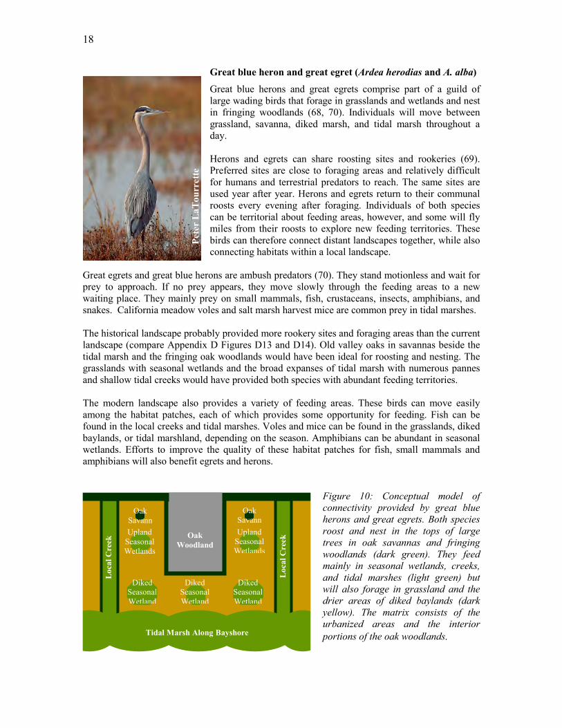
Great blue herons and great egrets comprise part of a guild of large wading birds that forage in grasslands and wetlands and nest in fringing woodlands (68, 70). Individuals will move between grassland, savanna, diked marsh, and tidal marsh throughout a day. Herons and egrets can share roosting sites and rookeries (69). Preferred sites are close to foraging areas and relatively difficult for humans and terrestrial predators to reach. The same sites are used year after year. Herons and egrets return to their communal roosts every evening after foraging. Individuals of both species can be territorial about feeding areas, however, and some will fly miles from their roosts to explore new feeding territories. These birds can therefore connect distant landscapes together, while also connecting habitats within a local landscape.
Great egrets and great blue herons are ambush predators (70). They stand motionless and wait for prey to approach. If no prey appears, they move slowly through the feeding areas to a new waiting place. They mainly prey on small mammals, fish, crustaceans, insects, amphibians, and snakes. California meadow voles and salt marsh harvest mice are common prey in tidal marshes. The historical landscape probably provided more rookery sites and foraging areas than the current landscape (compare Appendix D Figures D13 and D14). Old valley oaks in savannas beside the tidal marsh and the fringing oak woodlands would have been ideal for roosting and nesting. The grasslands with seasonal wetlands and the broad expanses of tidal marsh with numerous pannes and shallow tidal creeks would have provided both species with abundant feeding territories. The modern landscape also provides a variety of feeding areas. These birds can move easily among the habitat patches, each of which provides some opportunity for feeding. Fish can be found in the local creeks and tidal marshes. Voles and mice can be found in the grasslands, diked baylands, or tidal marshland, depending on the season. Amphibians can be abundant in seasonal wetlands. Efforts to improve the quality of these habitat patches for fish, small mammals and amphibians will also benefit egrets and herons.
Figure 10: Conceptual model of connectivity provided by great blue herons and great egrets. Both species roost and nest in the tops of large trees in oak savannas and fringing woodlands (dark green). They feed mainly in seasonal wetlands, creeks, and tidal marshes (light green) but will also forage in grassland and the drier areas of diked baylands (dark yellow). The matrix consists of the urbanized areas and the interior portions of the oak woodlands.
Pete
rLa
Tour
rette
Oak Woodland
Loc
alC
reek
Loc
alC
reek
Tidal Marsh Along Bayshore
Upland Seasonal Wetlands
Upland Seasonal Wetlands
Diked Seasonal Wetland
Diked Seasonal Wetland
Diked Seasonal Wetland
Oak Savann
Oak Savann
19
Northern harrier (Circus cyaneus)
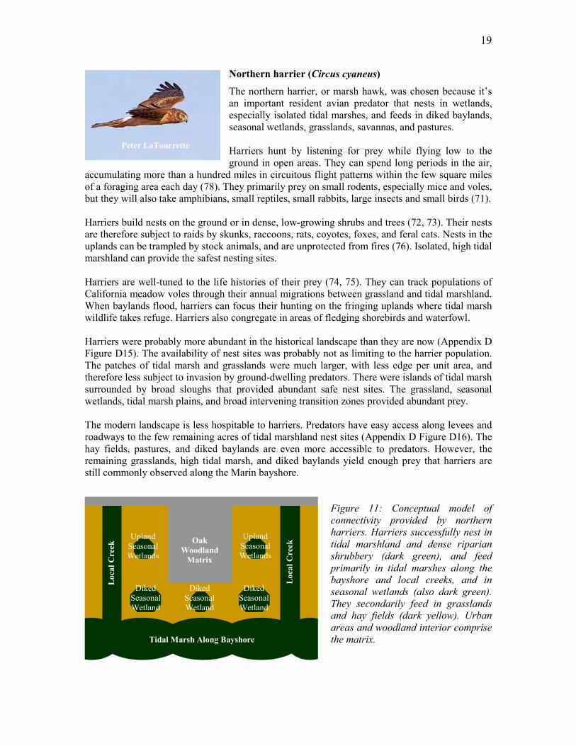
The northern harrier, or marsh hawk, was chosen because it’s an important resident avian predator that nests in wetlands, especially isolated tidal marshes, and feeds in diked baylands, seasonal wetlands, grasslands, savannas, and pastures. Harriers hunt by listening for prey while flying low to the ground in open areas. They can spend long periods in the air,
accumulating more than a hundred miles in circuitous flight patterns within the few square miles of a foraging area each day (78). They primarily prey on small rodents, especially mice and voles, but they will also take amphibians, small reptiles, small rabbits, large insects and small birds (71). Harriers build nests on the ground or in dense, low-growing shrubs and trees (72, 73). Their nests are therefore subject to raids by skunks, raccoons, rats, coyotes, foxes, and feral cats. Nests in the uplands can be trampled by stock animals, and are unprotected from fires (76). Isolated, high tidal marshland can provide the safest nesting sites. Harriers are well-tuned to the life histories of their prey (74, 75). They can track populations of California meadow voles through their annual migrations between grassland and tidal marshland. When baylands flood, harriers can focus their hunting on the fringing uplands where tidal marsh wildlife takes refuge. Harriers also congregate in areas of fledging shorebirds and waterfowl. Harriers were probably more abundant in the historical landscape than they are now (Appendix D Figure D15). The availability of nest sites was probably not as limiting to the harrier population. The patches of tidal marsh and grasslands were much larger, with less edge per unit area, and therefore less subject to invasion by ground-dwelling predators. There were islands of tidal marsh surrounded by broad sloughs that provided abundant safe nest sites. The grassland, seasonal wetlands, tidal marsh plains, and broad intervening transition zones provided abundant prey. The modern landscape is less hospitable to harriers. Predators have easy access along levees and roadways to the few remaining acres of tidal marshland nest sites (Appendix D Figure D16). The hay fields, pastures, and diked baylands are even more accessible to predators. However, the remaining grasslands, high tidal marsh, and diked baylands yield enough prey that harriers are still commonly observed along the Marin bayshore.
Figure 11: Conceptual model of connectivity provided by northern harriers. Harriers successfully nest in tidal marshland and dense riparian shrubbery (dark green), and feed primarily in tidal marshes along the bayshore and local creeks, and in seasonal wetlands (also dark green). They secondarily feed in grasslands and hay fields (dark yellow). Urban areas and woodland interior comprise the matrix.
Peter LaTourrette
Oak Woodland
Matrix
Loca
lCre
ek
Loca
lCre
ek
Tidal Marsh Along Bayshore
Upland Seasonal Wetlands
Upland Seasonal Wetlands
Diked Seasonal Wetland
Diked Seasonal Wetland
Diked Seasonal Wetland
20
Tree swallow (Tachycineta bicolor)
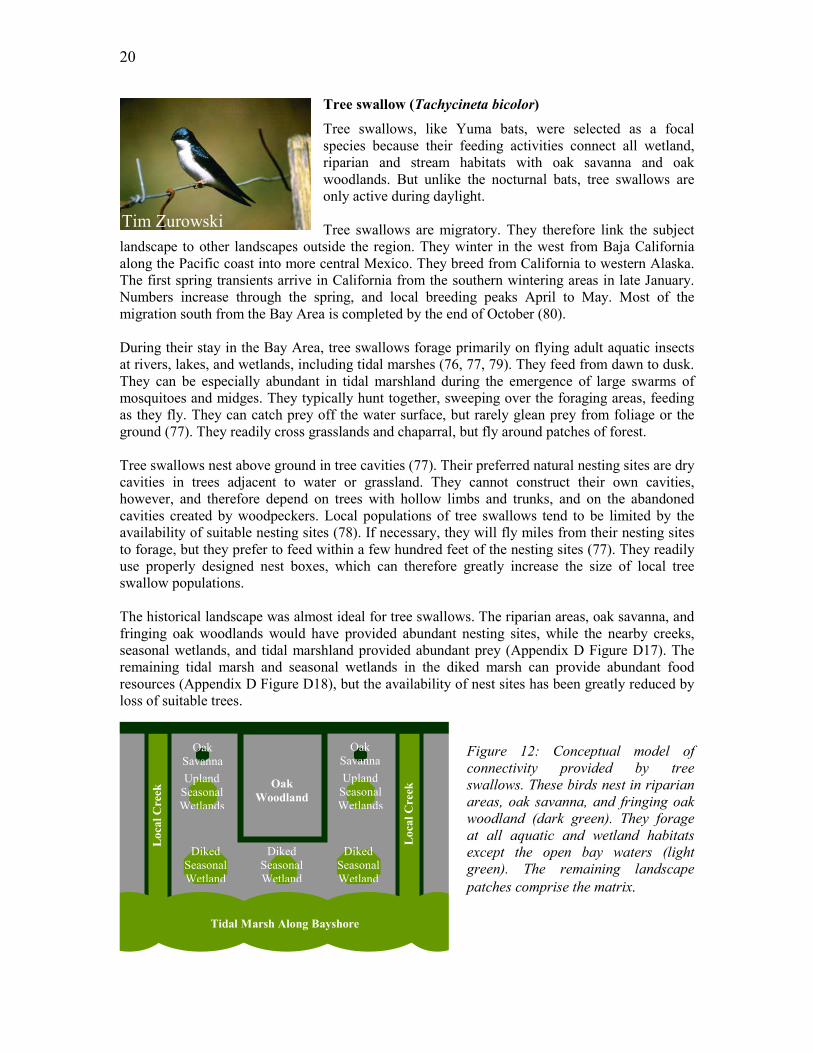
Tree swallows, like Yuma bats, were selected as a focal species because their feeding activities connect all wetland, riparian and stream habitats with oak savanna and oak woodlands. But unlike the nocturnal bats, tree swallows are only active during daylight. Tree swallows are migratory. They therefore link the subject
landscape to other landscapes outside the region. They winter in the west from Baja California along the Pacific coast into more central Mexico. They breed from California to western Alaska. The first spring transients arrive in California from the southern wintering areas in late January. Numbers increase through the spring, and local breeding peaks April to May. Most of the migration south from the Bay Area is completed by the end of October (80). During their stay in the Bay Area, tree swallows forage primarily on flying adult aquatic insects at rivers, lakes, and wetlands, including tidal marshes (76, 77, 79). They feed from dawn to dusk. They can be especially abundant in tidal marshland during the emergence of large swarms of mosquitoes and midges. They typically hunt together, sweeping over the foraging areas, feeding as they fly. They can catch prey off the water surface, but rarely glean prey from foliage or the ground (77). They readily cross grasslands and chaparral, but fly around patches of forest. Tree swallows nest above ground in tree cavities (77). Their preferred natural nesting sites are dry cavities in trees adjacent to water or grassland. They cannot construct their own cavities, however, and therefore depend on trees with hollow limbs and trunks, and on the abandoned cavities created by woodpeckers. Local populations of tree swallows tend to be limited by the availability of suitable nesting sites (78). If necessary, they will fly miles from their nesting sites to forage, but they prefer to feed within a few hundred feet of the nesting sites (77). They readily use properly designed nest boxes, which can therefore greatly increase the size of local tree swallow populations. The historical landscape was almost ideal for tree swallows. The riparian areas, oak savanna, and fringing oak woodlands would have provided abundant nesting sites, while the nearby creeks, seasonal wetlands, and tidal marshland provided abundant prey (Appendix D Figure D17). The remaining tidal marsh and seasonal wetlands in the diked marsh can provide abundant food resources (Appendix D Figure D18), but the availability of nest sites has been greatly reduced by loss of suitable trees.
Figure 12: Conceptual model of connectivity provided by tree swallows. These birds nest in riparian areas, oak savanna, and fringing oak woodland (dark green). They forage at all aquatic and wetland habitats except the open bay waters (light green). The remaining landscape patches comprise the matrix.
Tim Zurowski
Oak Woodland
Loc
alC
reek
Loc
alC
reek
Tidal Marsh Along Bayshore
Upland Seasonal Wetlands
Upland Seasonal Wetlands
Diked Seasonal Wetland
Diked Seasonal Wetland
Diked Seasonal Wetland
Oak Savanna
Oak Savanna
21
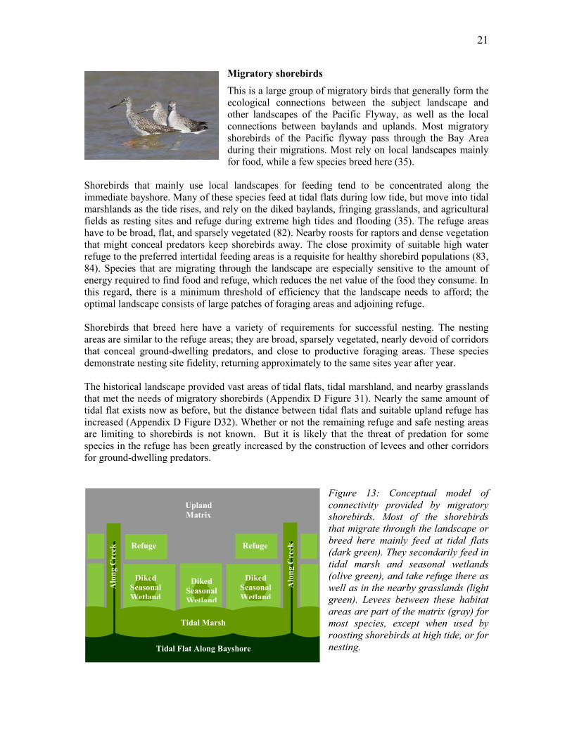
Migratory shorebirds
This is a large group of migratory birds that generally form the ecological connections between the subject landscape and other landscapes of the Pacific Flyway, as well as the local connections between baylands and uplands. Most migratory shorebirds of the Pacific flyway pass through the Bay Area during their migrations. Most rely on local landscapes mainly for food, while a few species breed here (35).
Shorebirds that mainly use local landscapes for feeding tend to be concentrated along the immediate bayshore. Many of these species feed at tidal flats during low tide, but move into tidal marshlands as the tide rises, and rely on the diked baylands, fringing grasslands, and agricultural fields as resting sites and refuge during extreme high tides and flooding (35). The refuge areas have to be broad, flat, and sparsely vegetated (82). Nearby roosts for raptors and dense vegetation that might conceal predators keep shorebirds away. The close proximity of suitable high water refuge to the preferred intertidal feeding areas is a requisite for healthy shorebird populations (83, 84). Species that are migrating through the landscape are especially sensitive to the amount of energy required to find food and refuge, which reduces the net value of the food they consume. In this regard, there is a minimum threshold of efficiency that the landscape needs to afford; the optimal landscape consists of large patches of foraging areas and adjoining refuge. Shorebirds that breed here have a variety of requirements for successful nesting. The nesting areas are similar to the refuge areas; they are broad, sparsely vegetated, nearly devoid of corridors that conceal ground-dwelling predators, and close to productive foraging areas. These species demonstrate nesting site fidelity, returning approximately to the same sites year after year. The historical landscape provided vast areas of tidal flats, tidal marshland, and nearby grasslands that met the needs of migratory shorebirds (Appendix D Figure 31). Nearly the same amount of tidal flat exists now as before, but the distance between tidal flats and suitable upland refuge has increased (Appendix D Figure D32). Whether or not the remaining refuge and safe nesting areas are limiting to shorebirds is not known. But it is likely that the threat of predation for some species in the refuge has been greatly increased by the construction of levees and other corridors for ground-dwelling predators.
Figure 13: Conceptual model of connectivity provided by migratory shorebirds. Most of the shorebirds that migrate through the landscape or breed here mainly feed at tidal flats (dark green). They secondarily feed in tidal marsh and seasonal wetlands (olive green), and take refuge there as well as in the nearby grasslands (light green). Levees between these habitat areas are part of the matrix (gray) for most species, except when used by roosting shorebirds at high tide, or for nesting.
Upland Matrix
Tidal Marsh
Alo
ngC
reek
Alo
ngC
reek
Diked Seasonal Wetland
Diked Seasonal Wetland
Diked Seasonal Wetland
Refuge Refuge
Tidal Flat Along Bayshore
22
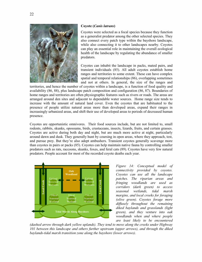
Coyote (Canis latrans)
Coyotes were selected as a focal species because they function as a generalist predator among the other selected species. They also connect every patch type within the bayshore landscape, while also connecting it to other landscapes nearby. Coyotes can play an essential role in maintaining the overall ecological health of the landscape by regulating the abundance of smaller predators. Coyotes can inhabit the landscape in packs, mated pairs, and transient individuals (85). All adult coyotes establish home ranges and territories to some extent. These can have complex spatial and temporal relationships (86), overlapping sometimes and not at others. In general, the size of the ranges and
territories, and hence the number of coyotes within a landscape, is a function of food quality and availability (86, 88), plus landscape patch composition and configuration (86, 87). Boundaries of home ranges and territories are often physiographic features such as rivers or roads. The areas are arranged around den sites and adjacent to dependable water sources. Home range size tends to increase with the amount of natural land cover. Even the coyotes that are habituated to the presence of people utilize natural areas more than developed areas, expand their ranges in increasingly urbanized areas, and shift their use of developed areas to periods of decreased human presence. Coyotes are opportunistic omnivores. Their food sources include, but are not limited to, small rodents, rabbits, skunks, opossums, birds, crustaceans, insects, lizards, fruits, and certain grasses. Coyotes are active during both day and night, but are much more active at night, particularly around dawn and dusk. They generally hunt by coursing in open areas, where they approach, test, and pursue prey. But they’re also adept ambushers. Transient coyotes generally scavenge more than coyotes in pairs or packs (85). Coyotes can help maintain native fauna by controlling smaller predators such as rats, raccoons, skunks, foxes, and feral cats (89). Coyotes have very few natural predators. People account for most of the recorded coyote deaths each year.
Figure 14: Conceptual model of connectivity provided by coyotes. Coyotes can use all the landscape patches. The riparian areas and fringing woodlands are used as corridors (dark green) to access seasonal wetlands, tidal marsh margins, and local creeks for foraging (olive green). Coyotes forage more diffusely throughout the remaining diked baylands and grasslands (light green), and they venture into oak woodlands when and where people are least likely to be encountered
(dashed arrow through dark yellow uplands). They tend to move along the creeks under Highway 101 between this landscape and others further upstream (upper arrows), and through the diked baylands-tidal marsh transition zone along the bayshore (lower arrows).
Oak Woodland
Loc
alC
reek
Loca
lCre
ek
Tidal Marsh Along Bayshore
Upland Seasonal Wetlands
Upland Seasonal Wetlands
Diked Seasonal Wetland
Diked Seasonal Wetland
Diked Seasonal Wetland
23
Discussion Essential ecological services are provided by landscapes with habitat patches that are inhabited and interconnected by stable populations of native plants and animals. Wetlands, streams, woodlands, and other habitat types provide surprisingly little ecological service in isolation. They require herbivores to maintain plant communities, predators to maintain populations of herbivores, burrowing animals to turn over and aerate the soils, birds to disperse seeds, etc. And many of the wildlife species that help maintain the landscape meet their habitat needs by moving among a variety of patches. Comparable amounts of ecological connectivity can be provided in different landscapes by different wildlife species, but persistent native biodiversity that is not overly threatened by people is an integral measure of landscape health. The health of a landscape can therefore be assessed as the amount of ecological connectivity among the habitat patches, and the connectivity can be assessed as the biological diversity that the landscape supports. The uplands and baylands of Marin County are intimately connected to each other and to other landscapes by populations of native wildlife that reside in the landscape or move through it during the normal course of their lives. Here we can find the tracks of coyotes chasing voles from wetlands into meadows, watch harriers gliding from grassland to tidal marsh, see flocks of water birds during their autumn migrations, and hear the springtime chorus of song sparrows. Some steelhead can still make their way up local creeks through the landscape to spawn in adjoining watersheds. This Marin bayshore landscape still supports important wildlife communities. But the level of wildlife support is tenuous. Survival of each focal species examined for this report is threatened by severe habitat alterations and ongoing land use practices that are inconsistent with the County’s goals of vital and sustainable ecosystems. Tidal marsh reclamation, ranching, and urbanization have carved up the landscape with buildings, levees and roadways, ditches, and fence lines. Agricultural practices have eliminated oak reproduction in historical savannahs and severely restricted the distribution of riparian forests. Most patches of habitat are smaller, dominated by edge effects, farther apart than they were, and degraded. The corridors for wildlife movement are rife with danger due to their reduced length, narrowness, lack of adequate refuge, or close association with developed lands. The risk of predation has increased for most prey, although some kinds of predators lack sufficient space for sustainable and suitable prey populations, or they lack breeding sites, or they are simply too threatened by people. Conserving the Marin bayshore landscape will require strengthening the ecological connectivity within the landscape and between it and other landscapes of the region. This in turn will require protecting existing habitat, enlarging some habitat patches, and/or improving their condition, while also improving the corridors for wildlife movement among the patches. There is little room for error. There is no excess of land for essential ecological services. All the remaining wildlife habitats are needed to secure the remaining ecological services of the landscape and to provide a basic framework of
24
habitat patches and corridors that can be enhanced to achieve the County’s goals for viable, sustainable ecosystems. It is important to recognize that the developed and undeveloped portions of the landscape are integral parts of the whole. It will be necessary in the future for local agencies to coordinate their land use management efforts to assure that the developed and undeveloped areas provide a higher level of ecological connectivity across the whole landscape than can be achieved if the areas continue to be managed as separate and unrelated to each other. In the meantime, it is essential to protect and to restore the ecological connectivity within all the undeveloped areas in ways that minimize the disconnection caused by existing developments. While we have focused on the essential need to conserve and restore ecological connectivity for the remaining undeveloped portions of the bayshore landscape, we recognize that efforts to conserve or enhance biological diversity for the landscape as a whole will need to accommodate major roadways as essential corridors for people, flood control to protect human life and property, and other societal needs that the landscape must provide. But these needs must not be met at the cost of ecological services or the County’s goals for vital, sustainable ecosystems will not be achieved. The efforts to protect and enhance ecological services will have to accommodate changes to the landscape itself. Recent forecasts of regional climate change suggest that the hydrology of creeks, the distribution and abundance of non-tidal wetlands, and the distribution and abundance of vegetation types will significantly change during the next century. The best way to address these changes is dedicating enough lands to ecological service to accommodate the range of climate change. There is no surplus of undeveloped lands to meet this need. The forecasts of sea level rise illustrate this point. As the Bay rises, the bayshore landscape will narrow. Marshes and grasslands could get squeezed against levees, roadways, and other developments. The conservation of biodiversity to secure essential ecological services may need to emphasize ecological connectivity among smaller habitat patches. Any future reductions in habitats caused by land use may eliminate the opportunity to conserve adequate habitat to offset the effects of sea level rise in the future. Agriculture and past conservation efforts have secured important opportunities to protect and even restore the native biodiversity of the bayshore landscape. Looking east from Highway 101 still brings the shoreline into view, and the East Bay hills across the Bay, and on a clear day, Mount Diablo. In between the Highway and the Bay are ranchlands and open spaces that hold the promise of ecological integrity and healthy landscapes. Good ecological health can be built into the future through careful landscape design and prudent management.
Recommendations This study was necessarily rapid and therefore somewhat preliminary. But, it revealed some fundamental recommendations for conserving and improving the landscape for all the life it can support, and for improving the quality of life for the people of Marin County and the Bay Area in general.
25
While there are sound scientific methods of data collection and analysis that might be employed in the future to provide additional information if needed, any additional studies are unlikely to alter the basic recommendations provided below.
• Avoid any further losses of wildlife habitat connectivity and function. Given the severe alterations and fragmentation of the landscape that have already happened, and the likely demands for habitat relating to climate change and especially sea level rise, any further fragmentation or isolation of wildlife habitat could significantly reduce future chances to secure vital, sustainable ecosystems along the Marin bayshore.
• Give way to the Bay. Give the Bay someplace to go. Sea level rise will accelerate. Walling-in the Bay with levees to prevent its landward transgression will ruin the Bay and the adjoining Bayshore landscape. Any consideration of how much of each valley bayward of Highway 101 should be dedicated to the Bay’s inevitable landward transgression should include the necessary linkages to adjoining grasslands, oak savannah, creeks, riparian zones, and other habitat types. Such consideration is likely to reveal that all the remaining undeveloped lands are needed to accommodate future changes in climate, including accelerated sea level rise.
• In the context of planning for landward transgression by the Bay, greatly increase the ecological connectivity along the bayshore. Tidal marshland should fringe the entire bayshore, including the tidal reach of every local creek.
• Greatly increase the connectivity between the tidal baylands and the upper watersheds. The opportunity exists to restore steelhead to local creeks, and to provide safe passage for terrestrial wildlife under and over across Highways 101 and 37. Wildlife crossings are common in other parts of the world. If dealt with properly, sea level rise and the landward transgression of the Bay will help facilitate the improved connectivity between the Bay and its watersheds.
• Extend broad corridors of riparian areas and oak savannas from the highways to the Bay. However, not all creeks should reach that far. The ones that don’t should end in willows. The historical landscape will show how creeks should flow.
• Protect and restore the valley oak savannas. Oaks can be planted in urban development if necessary. And discourage the cutting of standing dead oaks. Some large dead oaks and other tree snags are important ecological amenities.
While we strongly recommend no further fragmentation or isolation of wildlife habitat, we recognize that some conversion of habitat into developed areas or agriculture may be inevitable, and in that context we suggest the following basic ideas for minimizing the negative effects of development on ecological connectivity for the bayshore landscape.
• Any development adjoining a riparian area should include native riparian shrubs and trees within the development to increase its support of riparian ecology and to blur the ecological boundary between the developed areas and the undeveloped areas.
• Ban fences and walls in residential and other developed areas. The historic housing for officers at Hamilton Air Base now used to house Coast Guard personnel is a pretty good model for residential development that doesn’t break too many connections between woodlands and other habitat patches.
26
• Prohibit runoff from impervious surfaces from ever directly reaching creeks or the Bay. All water from impervious surfaces should be held in nearby grassy swales, seasonal wetlands, and groundwater recharge zones.
• Encourage the use of roosting and nesting boxes for bats and birds. They should adorn the larger habitat patches. Instructions for proper boxes are readily available.
• The footprint of any land developments should be constrained by the needs for focal species of wildlife to sustain their viable populations and to enable them to move securely and affectively among habitat patches throughout the landscape.
27
Citations 1. The Kentucky Environmental Quality Commission (EQC), 2003. 2002 Online
Public Opinion Poll on the Environment. http://www.eqc.ky.gov/NR/rdonlyres/FA03742C-D9A0-49E1-9A70-64ED6AF96CD3/0/onlinesurvey.pdf
2. Washington Statewide Public Opinion Poll, League of Conservation Voters, 1999. http://www.voteenvironment.org/programs/polling-research/state-polling/LCVEF_Washington-Poll_Oct1999.pdf
3. Communications Consortium Media Center. 1994. An Analysis of Public Opinion on Biodiversity and Related Environmental Issues, 1990-1994. Consultative Group on Biological Diversity. New York.
4. Jope, Katherine L. 1994. Paradigm of species conservation. Conservation Biology 8(4): 924-25.
5. Beden & Russonello Research and Communications. 1996. Current Trends in Public Opinion on the Environment: Environmental Compendium Update January 1996. Washington D.C.
6. Beden & Russonello Research and Communications. 2002. Americans and Biodiversity: New Perspectives in 2002. Washington D.C.
7. Peter H. Raven, 1997.Nature and Human Society: The Quest for a Sustainable World. National Research Council (NRC). D.C.
8. Convention on Biological Diversity, 1993. United Nations Environment Programme, United Nations, New York NY.
9. Daily, GC; S. Alexander, P.R. Ehrlich, L. Goulder, J. Lubchenco, P.A. Matson, H.A Mooney; S. Postel, S.H. Schneider, D. Tilman, and G.M. Woodwell 1997. Ecosystem Services: Benefits Supplied to Human Societies by Natural Ecosystems. Issues in Ecology [Issues Ecol.]. Vol. 1, no. 2, pp. 1-18. 1997.
10. Troll C. 1939. Luftbildplan and okologische bodenforschung. Zeitschraft der Gesellschaft fur Erdkunde Zu Berlin: 241–298.
11. Troll C. 1971. Landscape Ecology (Geoecology) and Biogeocenology - A Terminology Study. Geoforum 8/71: 43–46.
12. Wu, J. 2006. Landscape ecology, cross-disciplinarity, and sustainability science Landscape Ecology 21:1–4.
13. Forman, R.T.T. and M. Godron. 1986. Landscape Ecology. John Wiley and Sons, Inc., New York, NY, USA.
28
14. Forman, R.T.T. 1995. Land Mosaics: The Ecology of Landscapes and Regions. Cambridge University Press, Cambridge, UK.
15. Turner, M.G., R. H. Gardner and R. V. O'Neill, R.V. 2001. Landscape Ecology in Theory and Practice. Springer-Verlag, New York, NY, USA.
16. Hilty, J.A., W.Z. Lidicker Jr., and A.M. Merenlender. 2006. Corridor ecology the science and practice of linking landscapes for biodiversioty conservation. Island Press.
17. Zacharias, M. A., and J. C. Roff. 2001. Use of focal species in marine conservation and management: a review and critique. Aquatic Conservation: Marine and Freshwater Ecosystems 11:59-76.
18. Sustainability Working Group. 2001. Marin Countywide Plan Update 2001 Interim Guiding Principles. Marin County Community Development Agency, San Rafael, CA
19. Parker, I. and W.J. Matyas. 1981. CALVEG, A classification of California vegetation. U.S. Forest Service, Region 5. Mare Island, Vallejo CA.
20. Jones, C. G. and Lawton, J. H. (eds.). 1995. Linking Species and Ecosystems. Chapman and Hall, New York.
21. National Agriculture Imagery Program (NAIP). 2006. http://165.221.201.14/NAIP.html
22. USFWS. 2006. National Wetlands Inventory. http://www.fws.gov/nwi/
23. Collins, J.N., E. Stein, M. Sutula, R. Clark, A. E. Fetscher, L. Grenier, C. Grosso, and A. Wiskind. 2006. California rapid assessment method (CRAM) for wetlands and riparian areas volume 1: user’s manual version 4.2.1. http://www.cramwetlands.org/documents/CRAM%204.2.1_Vol1.pdf.
24. Multi-Resolution Land Characteristics Consortium ((MRLC). 1992. National Land Cover Data. http://landcover.usgs.gov/natllandcover.php
25. California Department of Fish and Game. 2006. The Vegetation Classification and Mapping Program. http://www.dfg.ca.gov/whdab/html/vegcamp.html.
26. Sawyer, J.O., and T. Keeler-Wolf. 1995. A manual of California vegetation. California Native Plant Society, Sacramento CA.
27. Dickins, E. F., U.S. Coast and Geodetic Survey (USCGS), 1897-98. Pacific Coast Resurvey of San Pablo Bay, California, Gallines Creek to Petaluma Creek, Register No. 2447. Washington, D.C. 1:10000. Courtesy of the National Ocean Service, Rockville, MD.
29
28. Grossinger, R. M., 1995. Historical evidence of freshwater effects on the plan form of tidal marshlands in the Golden Gate Estuary. Master's Thesis, Marine Sciences, University of California, Santa Cruz.
29. Grossinger, R. M., and R. A. Askevold, 2005. Historical analysis of California Coastal landscapes: methods for the reliable acquisition, interpretation, and synthesis of archival data. SFEI Contribution 396. San Francisco Estuary Institute, Oakland CA.
30. Grossinger, RM, RA Askevold, CJ Striplen, E Brewster, S Pearce, KN Larned, LJ McKee, and JN Collins, 2006. Coyote Creek Watershed Historical Ecology Study: Historical Condition, Landscape Change, and Restoration Potential in the Eastern Santa Clara Valley, California. SFEI Publication 426, San Francisco Estuary Institute, Oakland, CA.
31. Loring, T. R., General Land Office, 1852. Transcript of the Field Notes of a Survey of the Exterior Lines of Townships 2,3,4,5 North, Ranges 1,2,3,4,5 West. U.S. Department of the Interior, Bureau of Land Management Rectangular Survey, California, Vol. R210. Courtesy of Bureau of Land Management, Sacramento, CA.
32. Matthewson, R. C., General Land Office, 1858. Rancho San Pedro Santa Margarita y Las Gallinas. U.S. Department of the Interior, Bureau of Land Management Rectangular Survey, California, Township 2 North, Range 7 West. Courtesy of Bureau of Land Management, Sacramento, CA.
33. Rodgers, A. F., U.S. Coast Survey (USCS), 1854. San Francisco Bay, California, Plane Table Sheet XVII, Register No. 472. Washington, D.C. 1:10000. Courtesy of the National Ocean Service, Rockville, MD.
34. U.S. Geological Survey (USGS), 1914. Petaluma Quadrangle, California: 15-minute series (Topographic); 1:62,500. Courtesy of the Earth Science and Map Library, UC Berkeley.
35. Goals Project. 1999 Baylands Ecosystem Habitat Goals. A report of habitat recommendations prepared by the San Francisco Bay Area Wetlands Ecosystem Goals Project. U.S. Environmental Protection Agency, San Francisco, CA.
36. Wolfgang, G., H. Shellhammer, and H.T. Harvey. 1988. The ecology of the salt-marsh harvest mouse (Reithrodontomys raviventris) in a diked salt marsh Journal of Mammalogy, Vol. 69, No. 4: 696-703
37. Shellhammer, H.S. 1989. Salt marsh harvest mice, urban development, and rising sea levels. Conservation Biology, Vol. 3, No. 1:59-65
38. Johnson. R.F. 1956. Population structure in salt marsh song sparrows: part I. environment and annual cycle. Condor, Vol. 58, No. 1:24-44
30
39. Johnson. R.F. 1956. 1956. Population structure in salt marsh song aparrows: part II: density, age structure, and maintenance. Condor, Vol. 58, No. 4: 254-272
40. Botti, F., D. Warenycia and D. Becker. 1986. Utilization by salt marsh harvest mice Reithrodontomys raviventris halicoetes of a non-pickleweed marsh. Calif. Fish and Game 72:62-64.
41. Ferrel, G.T. 1966. Variation in blood group frequencies of song sparrows of the San Francisco Bay Region. Evolution 20:369-382.
42. Fisler, G.F. 1965. Adaptations and speciation in harvest mice of the marshes of San Francisco Bay. University of California Publication in Zoology volume 77.
43. Marshall, J.T. Jr. 1948. Ecological races of song sparrows in the San Francisco Bay region. Part I. Habitat and abundance. Condor 50:193-215.
44. Shellhammer, H.S., R. Duke, H.T. Harvey, V. Jennings, V. Johnson, and M. Newcomer. 1988. Salt marsh harvest mice in the diked salt marshes of southern San Francisco Bay. Wasmann J. Biol. 46:89-103.
45. U.S. Fish and Wildlife Service. 1984. Salt marsh harvest mouse and California clapper rail recovery plan.
46. Zetterquist, D. 1978. The salt marsh harvest mouse (Reithrodontomys raviventris raviventris) in marginal habitats. Wasmann J. Biology 12:135-153.
47. University of Californa Cooperative Extension. 2006. Division of Agriculture and Natural Resources web site: http://cecalaveras.ucdavis.edu/squirrel.htm.
48. Fitch. H.S. 1949. Ecology of the California ground squirrel on grazing land. Ecology, Vol. 30, No. 1: 112
49. Dobson, S.F. 1979. An experimental study of dispersal in the California ground squirrel. Ecology, Vol. 60, No. 6: 1103-1109.
50. Eaton. J. Best of enemies. Terrain. The Ecology Center. Terrain Web site: http://www.ecologycenter.org/terrain/article.php?id=13335.
51. Miller, B., R. Reading, J. Hoogland, T. Clark, G. Ceballos, R. List, S. Forrest, L. Hanebury, P. Manzano, J. Pacheco, and D. Uresk. 2000. The Role of prairie dogs as a keystone species: response to Stapp. Conservation Biology, Vol. 14 (1): Page 318.
52. Jameson, E.W., Jr. and H.J. Peeters. 1988. California Mammals. University of California Press, Berkeley, CA.
31
53. Hadaway, H.C. and J. R. Newman. 1971. Differential Responses of Five Species of Salt Marsh Mammals to Inundation. Journal of Mammalogy, Vol. 52, No. 4: 818-820
54. Thaeler, C.S. 1961. Variation in some salt-marsh populations of Microtus californicus. University of California Press, Berkeley Ca.
55. Howell, P.T. 1984. Use of salt marshes by meadow voles. Estuaries, Vol. 7, No. 2: 165-170.
56. Chapman, K., K. McGuiness and R. M. Brigham. 1994. Status of the Pallid bat. Wildlife Working Report No. WR-61.
57. Nagorsen, D.W., and R. M. Bingham. 1993. Bats of British Columbia. Royal British Columbia Museum Handbook.
58. Texas Parks and Wildlife, Nongame and Urban Program. 1994. The mammals of texas - online edition. http://www.nsrl.ttu.edu/tmot1/antrpall.htm
59. Johnston, D.S. and B. M. Fenton. 2001. Individual and population-level variability in diets of pallid bats (Antrozous pallidus). Journal of Mammalogy, vol. 82 (2): 362-373.
60. Brigham, R. M., H.D.J.N. Aldridge and R. L. Mackey. 1992. Variation in habitat use and prey selection by Yuma Bats, Myotis yumanensis. Journal of Mammalogy. 47:34-41.
61. Dalquest, W. W. 1947. Notes on the natural history of the bat, Myotis yumanensis, with a description of a new race. American Midland Naturalist 38:224-247.
62. Nagorsen, D. W. and R. M. Brigham. 1993. Bats of British Columbia, UBC Press, Vancouver, B.C.
63. Grindal, S. D. 1998. Habitat use by bats in second- and oldgrowth stands in the Nimpkish Valley, Vancouver Island. Pages 116-118 in J.A. Trofymow and A. MacKinnon, editors. Proceedings of a workshop on Structure, Process, and Diversity in Successional Forests of Coastal British Columbia, February 17-19, 1998, Victoria, British Columbia. Northwest Science, Vol. 72 (special issue No.2.
64. Nur. N. 2002. Tidal marsh song sparrows of San Francisco Bay. Quarterly Journal of PRBO Conservation Science. No. 128.
65. Collins, J. N., and Resh, V. H. 1985. Utilization of natural and man-made habitat by the salt marsh song sparrow Melospiza melodia samuelis (Baird). Calif. Fish Game 71:40-52.
32
66. Grenier, J. L. 2004. Ecology, behavior, and trophic adaptations of the salt marsh Song Sparrow Melospiza melodia samuelis: the importance of the tidal influence gradient. Ph.D. dissertation, University of California, Berkeley, CA.
67. Basham, M.P. and L. R. Mewaldt. 1987. Salt Water Tolerance and the Distribution of South San Francisco Bay Song Sparrows. Condor. Vol. 89, No. 4: 697-709.
68. Butler, R.W. 1997. The Great Blue Heron: A Natural History and Ecology of a Seashore Sentinel University of British Columbia Press, Vancouver.
69. Paine, J.M. 1972. A study of colonial nesting in the Great Blue Heron (Ardea herodias). Unpubl. B.Sc. thesis, Univ. Brit. Col., Vancouver.
70. McCrimmon, D. A., Jr., J. C. Ogden, and G. T. Bancroft. 2001. Great Egret (Ardea alba). In The Birds of North America, No. 570 (A. Poole and F. Gill, eds.). The Birds of North America, Inc., Philadelphia, PA.
71. Bernard, P., B. MacWhirter, R. Simmons, G.L. Hansen and P.C. Smith. 1987. Timing of breeding and the seasonal importance of passerine prey to northern harriers (Circus cyaneus). Can. J. Zool 65:1942-1946.
72. Bildstein, K. L. 1988. Northern harrier Circus cyaneus. Pp. 251 - 303 in R.S. Palmer, ed. vol 14. Handbook of North American Birds. Yale Univ. Press, New Haven, CT.
73. Hamerstrom, F. and M. Kopeny. 1981. Harrier nest-site vegetation. J. Raptor Res. 15(3):86-88.
74. Hamerstrom, F., F.N. Hamerstrom, and C.J. Burke. 1985. Effects of voles on mating systems in a central Wisconsin populations of harriers. Wilson Bull. 97(3):332-346.
75. Temeles, E.J. 1987. The relative importance of prey availability and intruder pressure in feeding territory size regulation by harriers, Circus cyaneus. Oecologia. 74:286-297.
76. Chapman, L. B. 1935. Studies of a tree swallow colony. Bird Banding 6:45-57.
77. Kuerzi, R. G. 1941. Life history studies of the tree swallow. Proc. Linn. Soc. N. Y. 52-53:1-52.
78. Rendell, WB, Robertson, RJ. 1990. Influence of forest edge on nest-site selection by tree swallows. Wilson Bulletin 102: 634-644.
79. McCarty, J. P. 1997. Aquatic community characteristics influence the foraging patterns of tree swallows. Condor 99:210-213.
33
80. Armstrong, A., E.C. Mendoza, and D. Winkler. 2005. Tree Swallow (Tachycineta bicolor). In The Riparian Bird Conservation Plan: a strategy for reversing the decline of riparian-associated birds in California. California Partners in Flight. http://www.prbo.org/calpif/htmldocs/riparian_v-2.html.
81. Armstrong, A., E.C. Mendoza, and D. Winkler. 2005. Tree Swallow (Tachycineta bicolor). In The Riparian Bird Conservation Plan: a strategy for reversing the decline of riparian-associated birds in California. California Partners in Flight. http://www.prbo.org/calpif/htmldocs/riparian_v-2.html.
82. Twedt, D. J., C. O. Nelms, V. E. Rettig, and S. R. Aycock. 1998. Shorebird use of managed wetlands in the Mississippi Alluvial Valley. Am. Midl. Nat. 140:140-152.
83. US Fish and Wildlife Service, 2003. Shorebirds waders of shores, wetland, and grasslands. USFWS Division of Migratory Bird Management, Arlington VA.
84. Erwin. R.M. 1996. Dependence of waterbirds and shorebirds on shallow-water habitats in the mid-Atlantic coastal region: An ecological profile and management recommendations Estuaries, Vol. 19, No. 2, Part A: Selected Papers from the First Annual Marine and Estuarine Shallow Water Science and Management Conference pp. 213-219.
85. Bekoff, M. 1979. Coyotes: biology, behavior, and management. Journal of Mammalogy, Vol. 60, No. 3: 658-659.
86. Chamberlain M.J., L. C. D., Leopold B.D. (2000). Spatial-use patterns, movements, and interactions among adult coyotes in central Mississippi. Canadian Journal of Zoology 78: 2087-2095.
87. Atwood, T. 2006. C. The influence of habitat patch attributes on coyote group size and interaction in a fragmented landscape. Canadian Journal of Zoology,Volume 84, Number 1: 80-87(8).
88. Prugh, L.R. 2005.Coyote prey selection and community stability during a decline in food supply. Oikos, Vol. 110 (2).
89. Henke, S. E. and F.C. Bryant. 1999. Effects of coyote removal on the faunal community in western Texas. Journal of wildlife management vol. 63, No. 4: 066-1081.
90. Sloan, D. 2006. Geology of the San Francisco Bay Region. California Natural History Guides, University of California Press, Berkeley CA.
91. Elaine K. Harding, Emiko Stevens. 2001. Using stable isotopes to assess seasonal patterns of avian predation across a terrestrial-marine landscape. Oecologia Vol. 129 (3): 436-444.
34
92. Bias, M.A. and M.L. Morrison. 2006. Habitat selection of the salt marsh harvest mouse and sympatric rodent species. Journal of Wildlife Management 70(3): 732–742.
93. Greenberg ,R.G. and J.E. Maldonado . Diversity and endemism in tidal marsh vertebrates. In: R.G. Greenberg , J.E. Maldonado, S. Droege, and M.V. McDonald (eds):Terrestrial vertebrates of tidal marshes: ecology, evolution, and conservation. Studies in Avian Biology. Forthcoming.
94. Bias, M. A. 1994. Ecology of the salt marsh harvest mouse in San Pablo Bay. Ph.D. Dissertation. Univ. Calif., Berkeley. 243pp.
95. South Bay Salt Pond Science Team. 2004. How restoration actions affect the salt marsh harvest mouse. South Bay Salt Pond Restoration Project, California Coastal Conservancy, Oakland CA. http://www.southbayrestoration.org/pdf_files/national_sci_panel/07SBSPSMHMdscrptCM100504.pdf.
96. Value of Biodiversity. 2006. Environmental Literacy Council. http://www.enviroliteracy.org/article.php/99.html.
97. Bryant, P. J. 2002. Biodiversity and conservation the origin, nature and value of biological diversity, the threats to its continued existence, and approaches to preserving what is left. Project of the Interdisciplinary Minor in Global Sustainability, School of Biological Sciences, University of California, Irvine CA. http://darwin.bio.uci.edu/~sustain/bio65/Titlpage.htm#Table%20of%20contents
98. Hector, A., J. Joshi, S. Lawler, E.M. Spehn, and A. Wilby. 2001. Conservation implications of the link between biodiversity and ecosystem functioning. Oecologia 129(4):624-628.
99. McCann, K.S. 2000. The diversity–stability debate. Nature vol. 405.
www.nature.com. 100. May, R. M. 1973. Stability and complexity in model ecosystems. Princeton
Univ. Press. Princeton NJ. 101. Tilman, D., J. Knops, D. Wedin, P. Reich, M. Ritchie, and E. Sieman. 1997. The
influence of functional diversity and composition on ecosystem processes. Science 277: 1300-1302.
102. Naeem, S., F.S. Chapin III, R. Costanza, P.R. Ehrlich, F.B. Golley, D.U.
Hooper, J.H. Lawton, R.V. O.Neill, H.A. Mooney, O.E. Sala, A.J. Symstad, and D. Tilman. 1999. Biodiversity and ecosystem functioning: maintaining natural life support processes. Issues in Ecology No. 4. http://www.epa.gov/watertrain/pdf/issue4.pdf.
35
Appendix A: Definitions of Key Terms "Biological Diversity" or “Biodiversity” means the variability among all living
organisms from all sources, including terrestrial, freshwater, marine and other aquatic ecosystems, and the ecological complexes of which they are part; this includes diversity within species, between species and of ecosystems (8).
“Ecosystem services” or “ecological services” are attributes of nature that are directly enjoyed, consumed, or used to yield human well-being (11), or the fundamental life-support services provided by natural ecosystems, without which civilization would cease to exist (10).
“Landscape Ecology” was originally defined as the study of complex causal relationships between biotic communities and their environments that are evident as landscape patterns (10, 11, 12). It has been defined more recently as the study of the distribution patterns of communities and ecosystems, the ecological processes that affect those patterns and changes in pattern and process over time (e.g., 14, 15), and more simply as the study of ecological systems having more than one type of biological community (16).
“Landscapes” are heterogeneous land areas of interacting elements in a repeating pattern (Forman 1986). Here are the most common landscape elements:
patches are relatively homogeneous areas that differ from their surroundings (often synonymous with patches of “Habitat Types”);
corridors are patches that allow organisms to move between other patches (they are essentially patches that connect other patches);
edges are boundaries between patches, corridors, and the matrix;
ecotones are transitional areas that straddle the edges between patches, corridors, and the matrix;
matrix is the most abundant element of the landscape in which patches and corridors are embedded;
buffers adjoin patches that protect them from disturbance and stress.
“Ecological Connectivity” or “Connectivity between Habitats” is a measure of the ability of organisms to move among separate patches of suitable habitat through edges, ecotones, corridors and matrix (16).
“Focal Species” are selected to address land management issues in a landscape context. Their habitat requirements are used to guide planning and management. They can include indicator species, keystone species (i.e., species having a disproportionate effect on their environment relative to their abundance), and other species chosen based on their resource requirements, conservation status, and/or sensitivity to management actions.

36
37
Appendix B: Science Team Biographies
Joshua N. Collins, Ph.D Dr. Collins received his Ph.D. in Entomological Sciences at the University of California at Berkeley and did post-doctoral studies in Geography and Ecology at the UC Berkeley and UC Davis. As an ecologist for the Pacific Gas and Electric Company, he conducted baseline ecological inventories and impact analyses in lacustrine, riverine and near-shore marine ecosystems. In private practice he designed wetland restoration projects. Dr. Collins currently directs the Wetlands Science Program at the San Francisco Estuary Institute, where he specializes in landscape ecology, regional ecological planning, and environmental monitoring. Joe Didonato Joe is a supervising wildlife ecologist for the east bay Regional Park District.
Geoffrey R. Geupel Geoff has over 23 years of experience in ornithological monitoring and conservation research. Geoff has a B.S. in Biology from Lewis and Clark College and has authored over 30 publications, many which have helped define bird-monitoring protocols throughout North America and Mexico. He has worked closely with private, state and federal agencies in California and other Western states to assess the impact of land management practices and restoration efforts on landbird populations. Geoff has taught numerous technical workshops on bird monitoring and conservation planning. He oversees 8 program areas including projects in The Great Valley, Eastern Sierra, Intermountain west shrub steppe, the Sierra Nevada, Latin America, and oak woodland and desert regions of California, that employ over 40 field biologists annually. He is currently co-Chair of California Partners in Flight, head of the Science Committee of the Riparian Habitat Joint Venture, member of the California State Steering Committee of the Intermountain West Joint Venture, technical committee member of the Central Valley Habitat Joint Venture, board member of the Sonora Joint Venture and member of the National Cowbird Advisory Council and International Important Bird Area Technical Committee. Geoff currently lives in Bolinas with his wife of 20 years Janet Kjelmyr and his two daughters and is a director on the Mesa Park Board.
J. Letitia Grenier, Ph.D. Dr. Grenier was born and raised in coastal California and maintains a lifelong interest in conservation of our native ecosystems. Dr. Grenier has been working in the tidal marshes of the San Francisco Bay estuary since 1999. She received her Ph.D. from the Environmental Science, Policy and Management Department at UC Berkeley, focusing on conservation biology and specializing in tidal marsh animal ecology. Her previous research has included tidal marsh food web structure and the relationship of song sparrow fitness and behavior to tidal marsh sub-habitats. Currently, she continues to study wetlands ecology and the bioaccumulation of contaminants in estuarine food webs, particularly mercury in tidal marsh animals. Dr. Grenier is in charge of monitoring biota in the South Bay Salt Ponds for the South Baylands Mercury Project.
38
Thomas E. Kucera, Ph.D.
Dr. Kucera received his Master’s degree in Resource Ecology from The University of Michigan and his Doctorate in Wildland Resource Science from the University of California, Berkeley. He has worked with a variety of agencies and organizations in the San Francisco Bay Area and throughout California on projects involving endangered species, ungulates, rare carnivores, raptors, wetlands, and wild turkeys. He recently finished an appointment as a research wildlife biologist at UC Berkeley, is a Project Manager with the Endangered Species Recovery Program at California State University, Stanislaus, and is a consultant for the California Department of Parks and Recreation and numerous private organizations. William Z. Lidicker, Ph.D. Dr. Lidicker Jr. is professor of integrative biology and curator of mammals emeritus at the Museum of Vertebrate Zoology, University of California, Berkeley. Bill Rainey, Ph.D. Dr. Rainey received his Doctorate in Zoology at the University of California, Berkeley, where he continues research on trophic exchange between terrestrial and aquatic communities in riparian habitats, landscape and seasonal patterns of prey production and bat community foraging activity along drainage networks; food web tracers; bat phylogeography and conservation biology. Steve Rottenborn, Ph.D. Dr. Rottenborn is a wildlife biologist and avian ecologist with a particular interest in wetland and riparian communities, as well as the effects of human activities on bird populations and communities. He received his Doctorate in Biological Sciences from Stanford University, studying the effects of urbanization on riparian bird and plant communities in the South San Francisco Bay area. As a senior ecologist for the ecological consulting firm H. T. Harvey & Associates, Steve has worked on hundreds of public and private projects in the San Francisco Bay area and beyond involving impact assessment, NEPA/CEQA documentation, endangered species issues, mitigation, and habitat restoration.
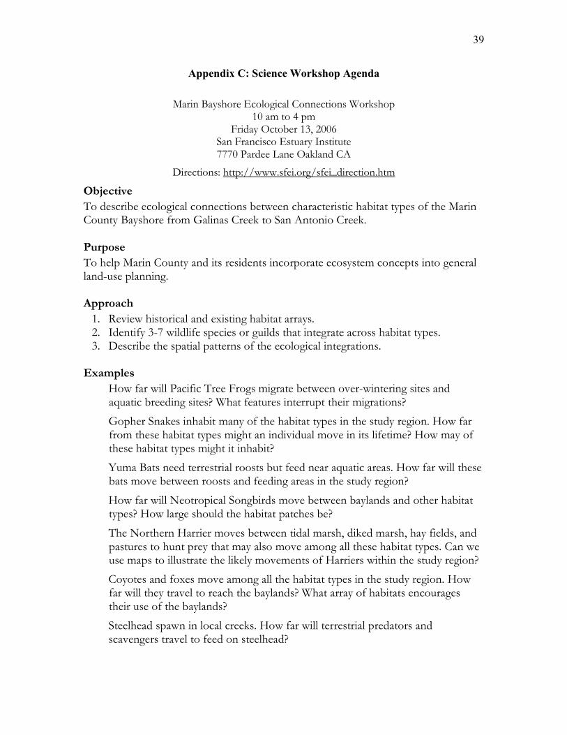
39
Appendix C: Science Workshop Agenda
Marin Bayshore Ecological Connections Workshop 10 am to 4 pm
Friday October 13, 2006 San Francisco Estuary Institute 7770 Pardee Lane Oakland CA
Directions: http://www.sfei.org/sfei_direction.htm
Objective To describe ecological connections between characteristic habitat types of the Marin County Bayshore from Galinas Creek to San Antonio Creek. Purpose To help Marin County and its residents incorporate ecosystem concepts into general land-use planning. Approach
1. Review historical and existing habitat arrays. 2. Identify 3-7 wildlife species or guilds that integrate across habitat types. 3. Describe the spatial patterns of the ecological integrations.
Examples
• How far will Pacific Tree Frogs migrate between over-wintering sites and aquatic breeding sites? What features interrupt their migrations?
• Gopher Snakes inhabit many of the habitat types in the study region. How far from these habitat types might an individual move in its lifetime? How may of these habitat types might it inhabit?
• Yuma Bats need terrestrial roosts but feed near aquatic areas. How far will these bats move between roosts and feeding areas in the study region?
• How far will Neotropical Songbirds move between baylands and other habitat types? How large should the habitat patches be?
• The Northern Harrier moves between tidal marsh, diked marsh, hay fields, and pastures to hunt prey that may also move among all these habitat types. Can we use maps to illustrate the likely movements of Harriers within the study region?
• Coyotes and foxes move among all the habitat types in the study region. How far will they travel to reach the baylands? What array of habitats encourages their use of the baylands?
• Steelhead spawn in local creeks. How far will terrestrial predators and scavengers travel to feed on steelhead?
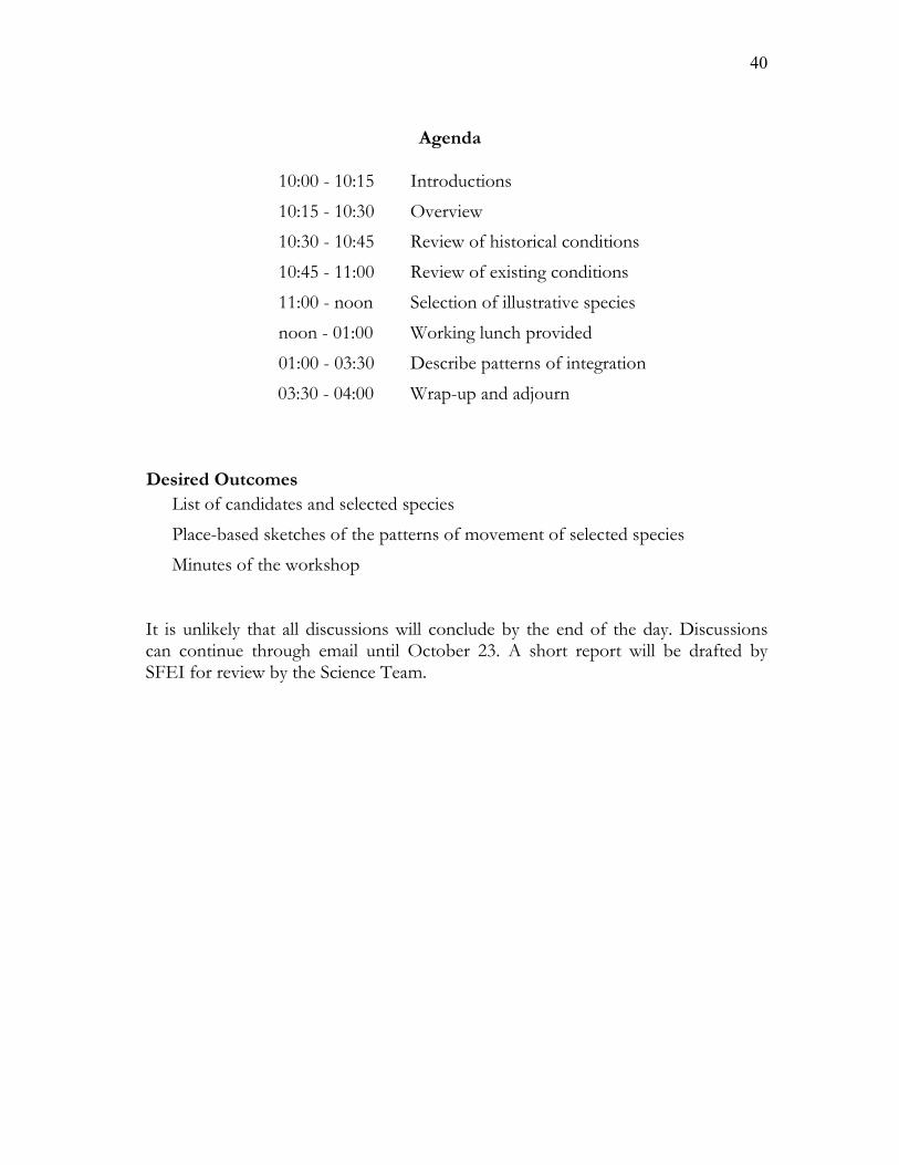
40
Agenda
10:00 - 10:15 Introductions 10:15 - 10:30 Overview 10:30 - 10:45 Review of historical conditions 10:45 - 11:00 Review of existing conditions 11:00 - noon Selection of illustrative species noon - 01:00 Working lunch provided 01:00 - 03:30 Describe patterns of integration 03:30 - 04:00 Wrap-up and adjourn
Desired Outcomes • List of candidates and selected species • Place-based sketches of the patterns of movement of selected species • Minutes of the workshop
It is unlikely that all discussions will conclude by the end of the day. Discussions can continue through email until October 23. A short report will be drafted by SFEI for review by the Science Team.
41
Appendix D: Specific Mapping Rules
1. Salt Marsh Harvest Mouse
Breeds and feeds in tidal marsh, excluding pannes and channels, and portions of diked marsh with abundant salt marsh vegetation. Refuge from flooding extends 20m into uplands and dry portions of diked marsh that adjoin breeding and feeding habitat.
2. California Ground Squirrel
Breed and feeds in coastal oak savanna, oak woodland, and grasslands. Feeding extends 20m into diked marsh and tidal marsh that adjoins breeding habitat. Colonizes levees in modern landscape.
3. California Meadow Vole
Breeds and feeds in coastal oak savanna, valley oak savanna, and grasslands during wet season. Distribution in these habitat patches may not be uniform but this was ignored for this mapping exercise. A 100m buffer was applied to the oak woodlands to account for their wet season movement into the lower limits of this patch type. Breeds and feeds in dike marsh and tidal marsh, except for pannes and channels, during the dry season.
4. Pallid Bat
Breeds and feeds in coastal oak savanna and valley oak savanna. A 50m buffer was applied to the lower limits of oak woodlands to account for roosting in this patch type. The distribution of roosts among built structures in patches of rural and urban development is localized and was ignored in this mapping exercise.
5. Yuma Bat
Feeds at all aquatic and wetland patch types except the open waters of the Bay, including tidal marsh, dike marsh, seasonal wetlands, riparian areas, streams, agricultural ditches, lakes, stock ponds, and treatment ponds. Roosts mostly in coastal oak savanna, valley oak savanna, and riparian areas. Use of built structures is common enough that urban development was included in the map of roosting habitat. A 50m buffer was applied to the lower limit of the oak woodlands to account for occurrence of roosts in fringing woodlands.
6. Song Sparrows
Breeds and feeds in tidal marsh and adjoining riparian areas. The upstream distribution of the intertidal subspecies or its genetic influence is unknown and was not represented in this mapping exercise. A 50m buffer was applied to the breeding and feeding habitat to account for the need to protect the habitat from marauding predators and to account for the tendency for song sparrows to venture into adjoining habitat patches to feed.
42
7. Herons and Egrets
Nests in coastal oak savanna, valley oak savanna, and Eucalyptus groves, and the lower limits of oak woodlands. Feeds mainly in tidal marsh (including pannes and channels), tidal flats, diked marsh, seasonal wetlands, steams, and grasslands.
8. Northern Harrier
Breeds and feeds mainly in tidal marsh (excluding large panes), diked marsh, and seasonal wetlands. Feeds secondarily in grasslands, pasture and some agricultural fields. A 50m buffer was applied to the feeding patches to account for the marginal hunting by harriers in adjoining patches.
9. Tree Swallow
Nests mainly in coastal oak savanna, valley oak savanna, riparian areas, and Eucalyptus groves. A buff of 50m was applied to the lower limits of oak woodlands to account for the nesting in the margins of this patch type. Feeds at all aquatic and wetland patches except open bay waters and tidal flats. Foraging habitats include tidal marsh (pannes included), diked marsh, streams, seasonal wetlands, lakes, stock ponds, and treatment ponds. A 50m buffer was applied to the lower limits of oak woodlands to account for roosting in fringing woodlands.
10. Migratory Shorebirds and Coyotes
Individuals of these focal species range beyond the subject landscape. Maps of their distribution within the landscape were therefore not developed. One or more migratory shorebird species feeds or takes refuge in most of the landscape patch types except oak woodlands and urban development. Individual coyotes forage throughout the landscape.
43
Appendix D: Maps of past and present distributions of focal species in the Marin bayshore landscape
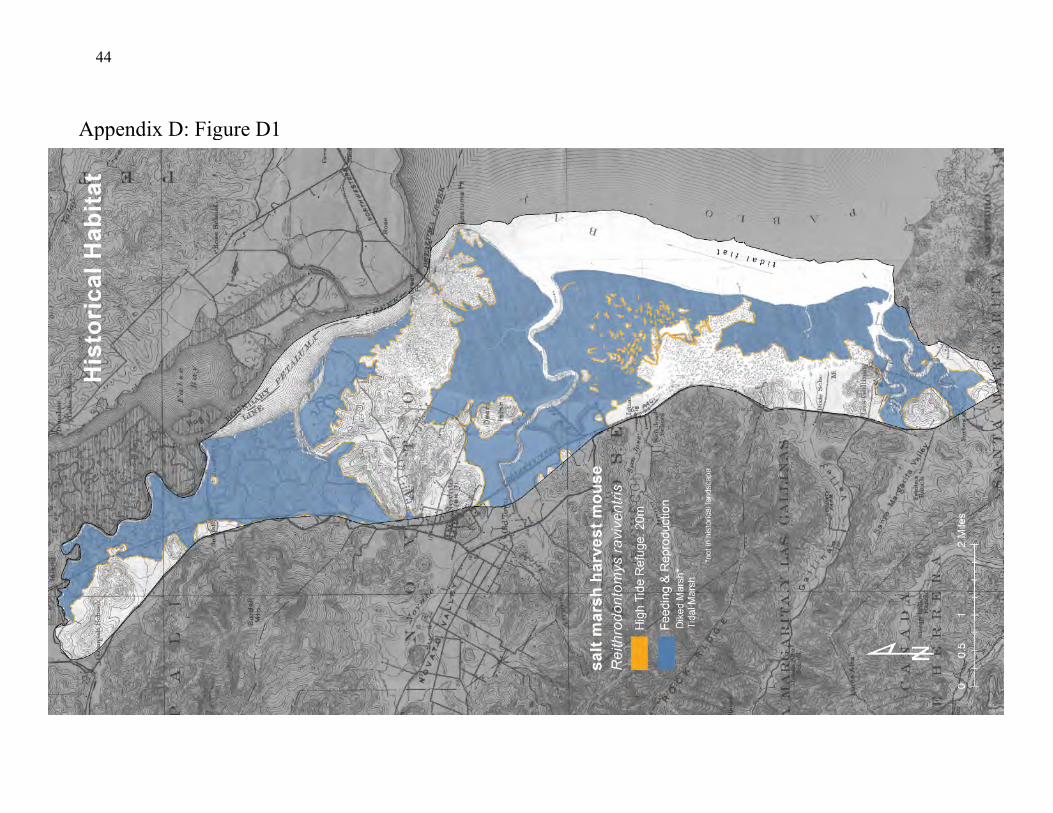
44
Appendix D: Figure D1
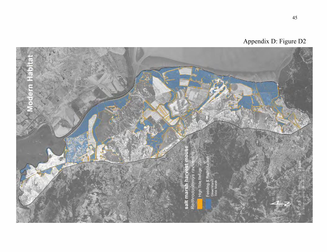
45
Appendix D: Figure D2
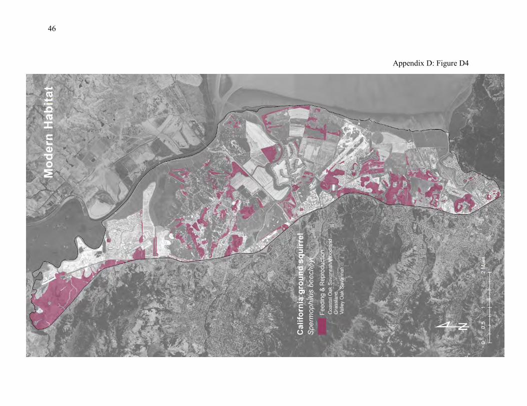
46
Appendix D: Figure D4
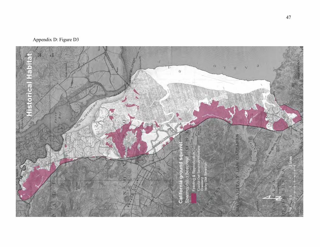
47
Appendix D: Figure D3
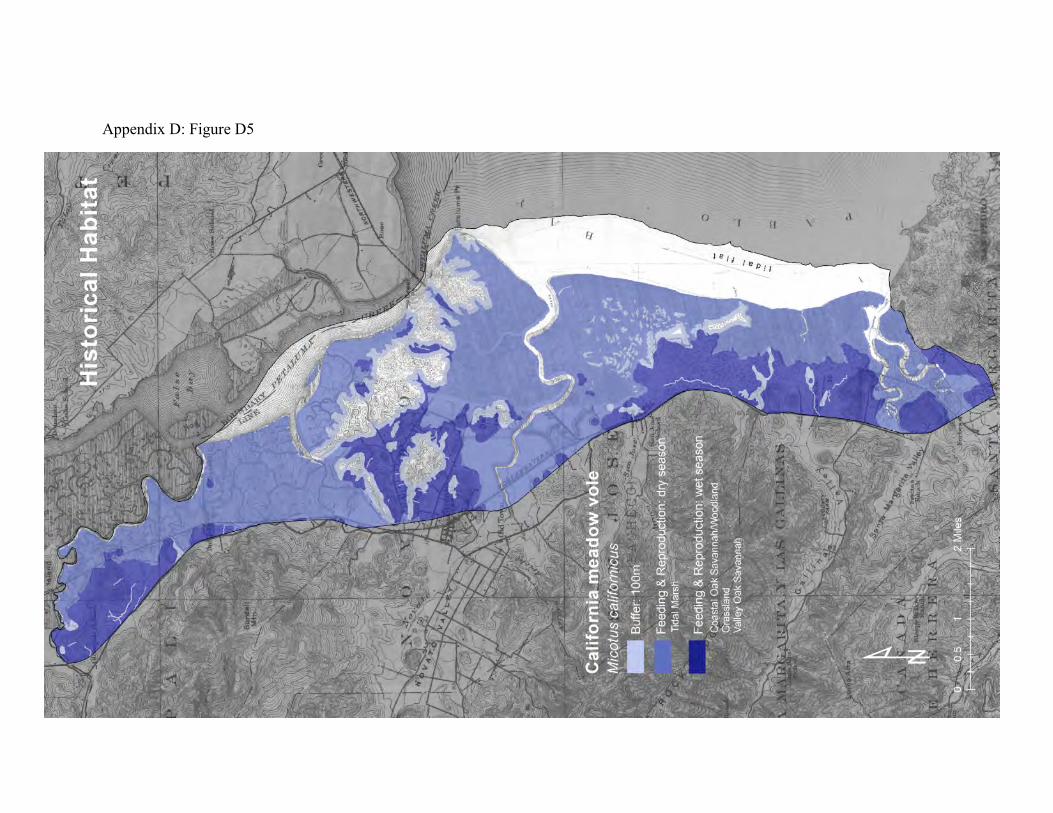
Appendix D: Figure D5
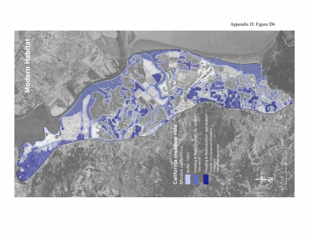
Appendix D: Figure D6
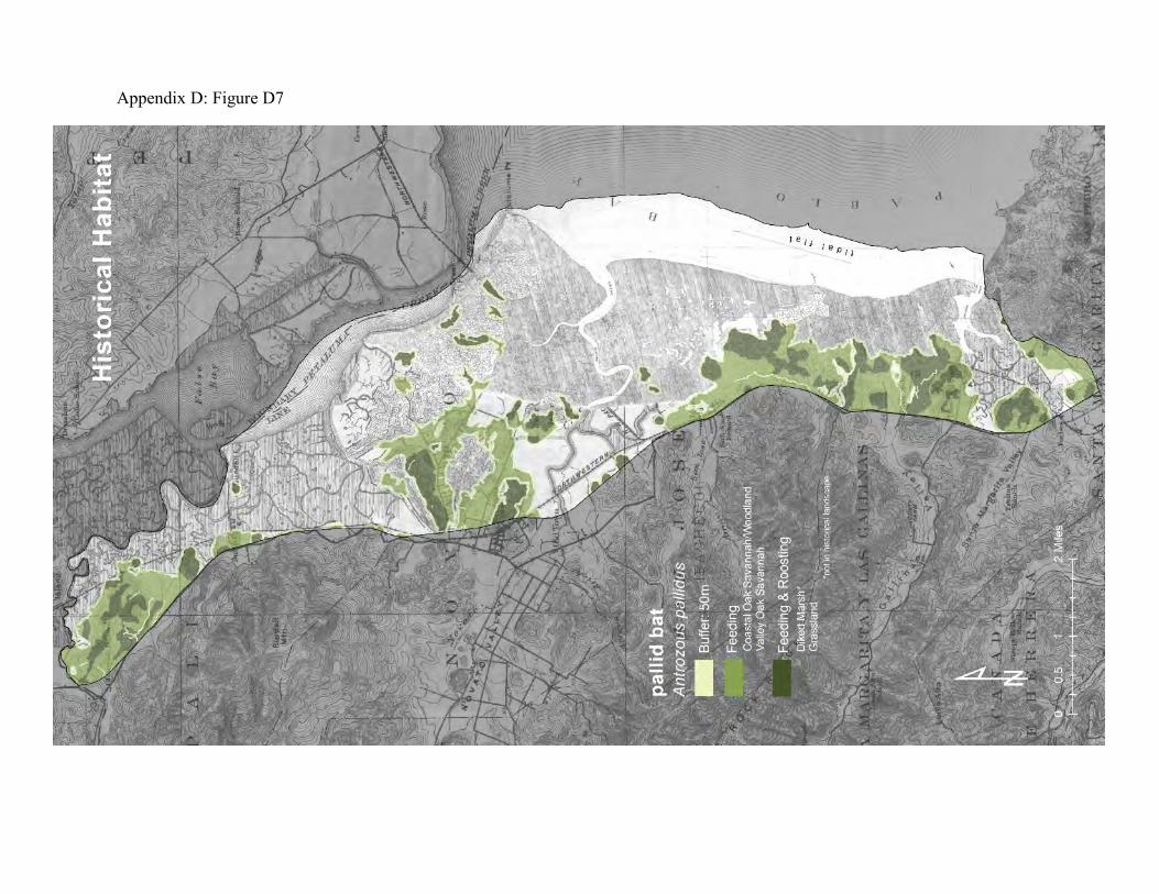
Appendix D: Figure D7
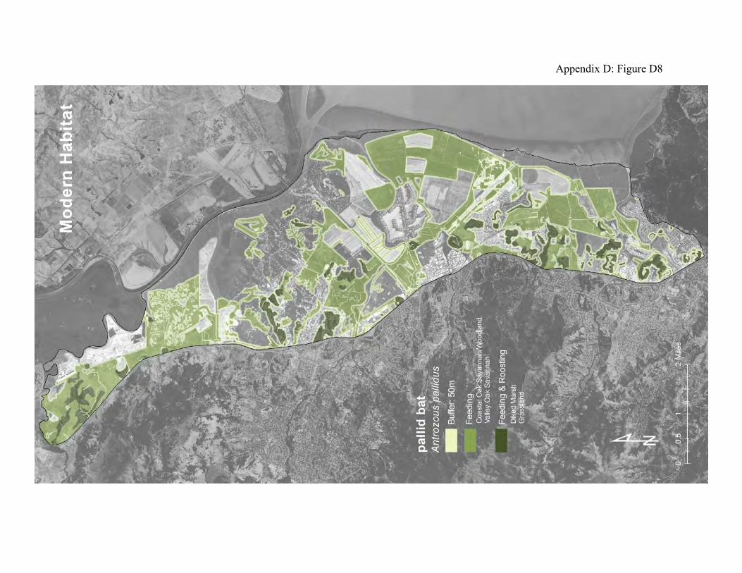
Appendix D: Figure D8
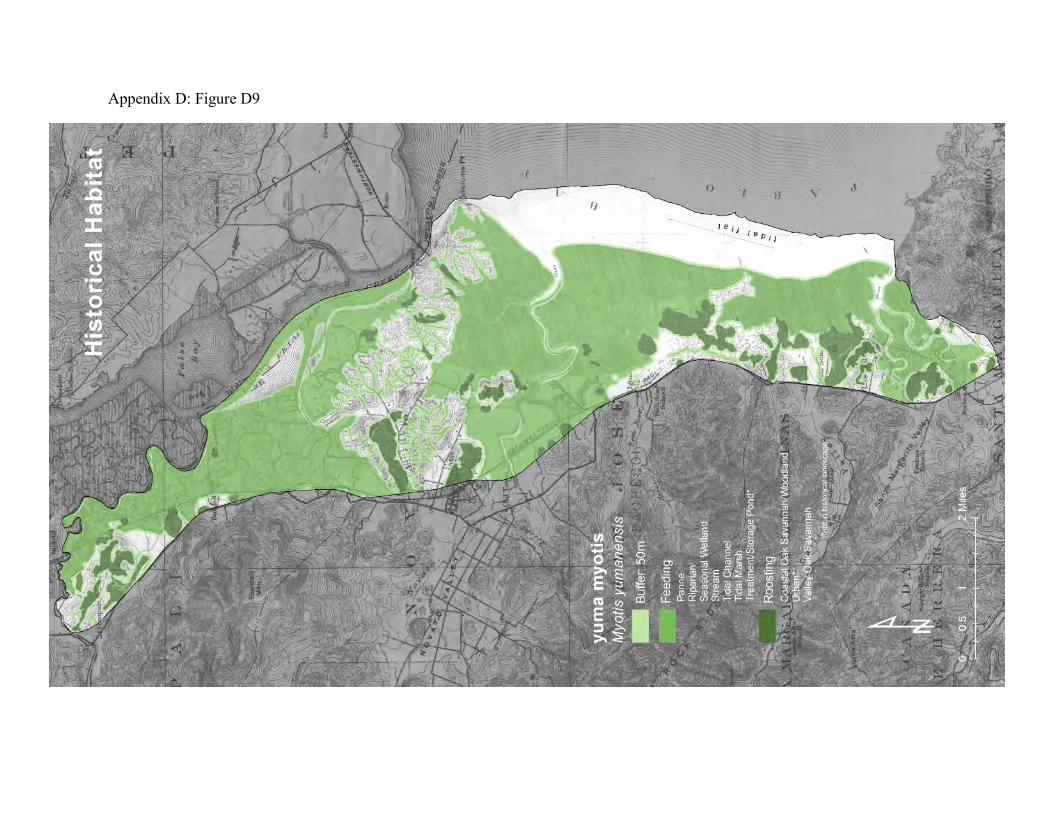
Appendix D: Figure D9
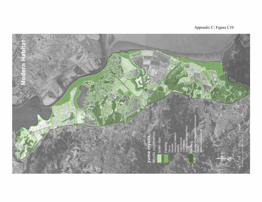
Appendix C: Figure C10
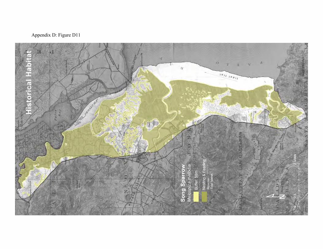
Appendix D: Figure D11
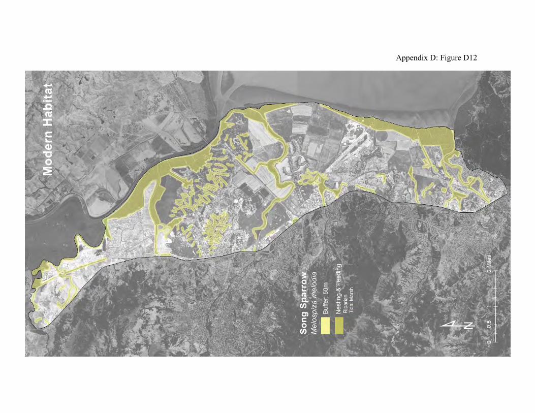
Appendix D: Figure D12
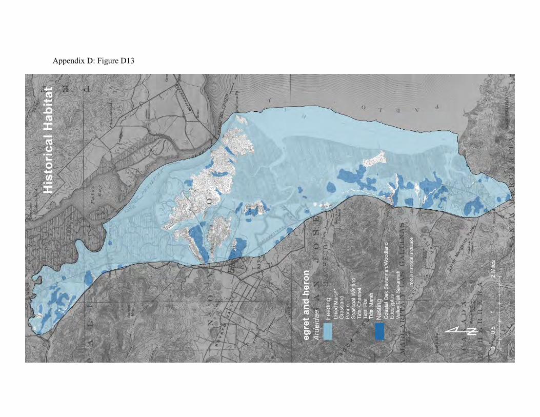
Appendix D: Figure D13
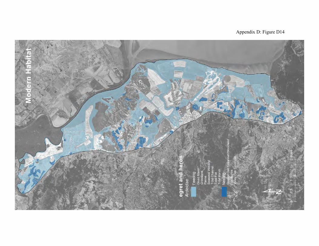
Appendix D: Figure D14
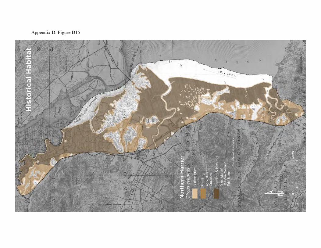
Appendix D: Figure D15
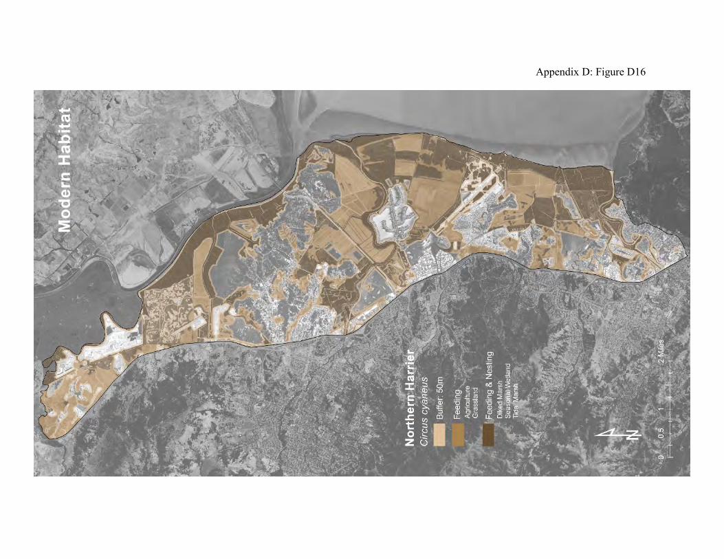
Appendix D: Figure D16
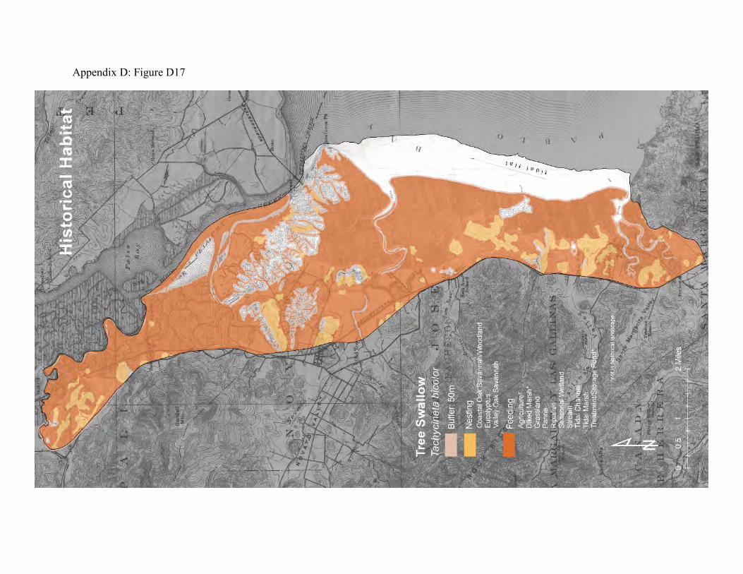
Appendix D: Figure D17

Appendix D: Figure D18