Embed Size (px)
Citation preview
ÉCOLE DE TECHNOLOGIE SUPÉRIEURE UNIVERSITÉ DU QUÉBEC
THESIS PRESENTED TO ÉCOLE DE TECHNOLOGIE SUPÉRIEURE
IN PARTIAL FULFILLMENT OF THE REQUIREMENTS FOR A MASTER’S DEGREE WITH THESIS IN AUTOMATIC MANUFACTURING
ENGINEERING M.A.Sc.
BY Sayed Salman NOURBAKHSH
VALIDATION OF A VIRTUAL PROTOTYPING METHOD USING COMPUTED TORQUE AND ILC AS CONTROLLERS ON A PARALLEL ROBOT
MONTREAL, MARCH 14TH, 2016
© Copyright Salman Nourbakhsh, 2016 All rights reserved.
© Copyright
Reproduction, saving or sharing of the content of this document, in whole or in part, is prohibited. A reader
who wishes to print this document or save it on any medium must first obtain the author’s permission.

THIS THESIS HAS BEEN EVALUATED
BY THE FOLLOWING BOARD OF EXAMINERS Mr. Guy Gauthier, Thesis Supervisor Génie de la production automatisée, at École de technologie supérieure Mr. Pascal Bigras, Thesis Co-supervisor Génie de la production automatisée, at École de technologie supérieure Mr. Vincent Duchaine, Chair, Board of Examiners Génie de la production automatisée, at École de technologie supérieure Mr. Maarouf Saad, Member of the jury Génie électrique, at École de technologie supérieure
THIS THESIS WAS PRESENTED AND DEFENDED
IN THE PRESENCE OF A BOARD OF EXAMINERS AND THE PUBLIC
ON MARCH 8TH, 2016
AT ÉCOLE DE TECHNOLOGIE SUPÉRIEURE


ACKNOWLEDGMENTS
During my master’s I learned a great deal in my field of study, but my most valuable learning
experiences came from the people in my life.
I must first thank my supervisor Dr. Guy Gauthier, and my Co-supervisor Dr. Pascal Bigras
for the trust and confidence they showed in me. What has been done here would not be
possible without their contributions.
Next I must thank my family for all their support. My parents and siblings helped me
overcome all the potential problems of immigration. I will always be grateful to them for
giving me the peace of mind I needed to concentrate on my work.
I can’t neglect my welcoming friends in Montreal. The fun environment they created was a
great source of energy. I am particularly indebted my friends Jean-Philippe Roberge and Eric
Boutet, who helped me complete a project at Hydro-Quebec, develop the chapter on virtual
prototyping, and set up the robot I used for this work.
To Dr. Looper and Dr. Shekarian, thank you for helping me to successfully continue my
education in a foreign country. I want to also express my gratitude to my friend, Kate Stern,
who helped me edit this thesis.
Finally I want to say thank you to Canada, and to Montreal. Here I felt reborn with hope and
motivation. To everyone mentioned here, and all those who have touched my life, I hope I
can someday repay even a small part of your kindness.


VALIDATION OF A VIRTUAL PROTOTYPING METHOD USING COMPUTED TORQUE AND ILC AS CONTROLLERS ON A PARALLEL ROBOT
Sayed Salman NOURBAKHSH
SUMMARY
This thesis validates a new method of virtual prototyping: a macro that automatically
generates a dynamic model from CATIA V6 and exports the model to SimMechanics. Until
now, engineers who need to verify their design with a dynamic model have either had to
calculate it by hand, or manually input all the necessary parameters in SimMechanics or
other software. Both of these methods are time-consuming and often lead to mistakes. To
demonstrate the relative difficulty of the hand-calculation method, we begin by presenting
our dynamic model of a four-bar parallel robot that we calculated using the Lagrange
method. At this stage we also calculated a computed torque controller that is used later when
comparing the performance of the macro-generated dynamic model to the actual robot. The
rest of our thesis shows how the new macro replaces both the hand-calculation and manual-
entry methods of dynamic modeling, and vastly simplifies the task of calculating the
computed-torque controller. We used the macro to export a dynamic model to SimMechanic,
where we then added a sensor and actuator to complete the dynamic model of our four-bar
parallel robot. The macro-generated model was tested in simulations using three
combinations of controller: computed torque alone, computed torque with P-type iterative
learning control (ILC), and computed torque with PD-type ILC. The third combination
produced the best results, that is, the lowest error value. To validate the performance of the
model, we then tested the performance of the real robot using the same three combinations of
controllers. Note that the computed torque used here is the one that was generated by the
macro. Again the results show that the combination of PD-type ILC and computed torque
functions best. However, the error was bigger in the practical experiment than it was in the
simulation, which used the macro-generated dynamic model. This difference is likely
because our dynamic model does not consider several factors that affect the real robot, such
as friction, the mass of screws and bolts, the moment of inertia of the rotor and pulleys, and
VIII
the stiffness of the timing belt. For the sake of simplicity, our dynamic model was not
intended to take all these factors into account. Therefore, the fact that the simulation results
closely match those of the practical experiment serves to validate this new method of virtual
prototyping.
Keywords: Validation, Virtual prototyping, Computed torque control, Iterative learning control, ILC, CATIA V6, SimMechanics.

VALIDATION D'UNE MÉTHODE DE PROTOTYPAGE VIRTUEL EN UTILISANT COUPLE PRÉ-CALCULÉ ET ILC COMME CONTRÔLEURS SUR UN ROBOT
PARALLÈLE
Sayed Salman NOURBAKHSH
RÉSUMÉ
Ce mémoire valide une nouvelle méthode de prototypage virtuel: une macro qui génère
automatiquement un modèle dynamique de CATIA V6 et exporte le modèle vers
SimMechanics. Jusqu'à présent, les ingénieurs qui avaient besoin de vérifier leur conception
d'un modèle dynamique devaient effectuer les calculs à la main, ou saisir manuellement tous
les paramètres nécessaires à SimMechanics ou d'autres logiciels. Ces deux méthodes sont
longues et conduisent souvent à des erreurs. Pour démontrer la difficulté relative de la
méthode analytique, nous commençons par présenter notre modèle dynamique d'un robot à
quatre barres parallèles, que nous avons calculé en utilisant la méthode de Lagrange. A ce
stade, nous avons aussi calculé un contrôleur de commande de couple pré-calculé qui sera
utilisé par la suite pour être comparé avec les performances du modèle dynamique généré par
la macro au robot réel. La suite de ce mémoire montrera comment la nouvelle macro
remplacera à la fois le calcul analytique et la saisie manuelle des paramètres du modèle
dynamique, et simplifiera ainsi considérablement la tâche de calcul de contrôleur de couple
pré-calculé. Nous avons utilisé la macro pour exporter le modèle dynamique vers
SimMechanic, où nous avons ajouté un capteur et un actionneur pour compléter le modèle
dynamique de notre robot à quatre barres parallèles. Le modèle généré par la macro a été
testé dans des simulations différentes, utilisant trois combinaisons de contrôleur : couple pré-
calculé seul, couple pré-calculé avec la commande d'apprentissage itératif (ILC) de type P, et
le couple pré-calculé avec l’ILC de type PD. La troisième combinaison a produit les
meilleurs résultats en donnant la valeur d'erreur la plus faible. Pour valider les performances
du modèle, nous avons ensuite testé les performances du robot réel en utilisant les trois
mêmes combinaisons de contrôleurs. A noter que le couple pré-calculé utilisé ici est celui qui
a été généré par la macro. Là encore, les résultats montrent que la combinaison de l’ILC de
type PD avec le couple pré-calculé est la meilleure des trois combinaisons. Cependant,
l'erreur est plus grande dans l'expérience pratique qu’elle ne l’est dans la simulation qui a
X
utilisé le modèle dynamique généré par la macro. Cette différence vient probablement du fait
que notre modèle dynamique ne considère pas certains facteurs qui influent sur le robot réel,
tels que le frottement, la masse des vis et des boulons, le moment d'inertie du rotor et des
poulies, et la rigidité de la courroie de distribution. En effet par souci de simplicité, nous
avions choisi de ne pas prendre en compte tous ces facteurs pour notre modèle dynamique.
Par conséquent, le fait que les résultats de la simulation correspondent étroitement à celles de
l'expérience pratique permet de valider cette nouvelle méthode de prototypage virtuel.
Mots clés: Validation, Prototypage virtuel, Couple pré-calculé, Commande d’apprentissage itératif, ILC, CATIA V6, SimMechanics.

TABLE OF CONTENT
Page
INTRODUCTION ...................................................................................................................23
REVIEW OF LITERATURE ............................................................................27 CHAPTER 11.1 Robots ..........................................................................................................................27
1.1.1 Serial robots .............................................................................................. 27 1.1.2 Parallel robots ........................................................................................... 28
1.2 Virtual prototyping.......................................................................................................29 1.3 Iterative learning control ..............................................................................................29
1.3.1 Iterative learning control definition .......................................................... 31 1.3.2 Iterative learning control history ............................................................... 31 1.3.3 Assumptions used for ILC ........................................................................ 33
ROBOT MODELING .......................................................................................35 CHAPTER 22.1 Introduction ..................................................................................................................35 2.2 Kinematic model ..........................................................................................................36
2.2.1 Direct kinematic ........................................................................................ 36 2.2.2 Singularities .............................................................................................. 40
2.3 Dynamic model ............................................................................................................40 2.4 Trajectory .....................................................................................................................51 2.5 Command law ..............................................................................................................52
2.5.1 Computed torque ....................................................................................... 52 2.6 Validation of the model ...............................................................................................55
VIRTUAL PROTOTYPING .............................................................................59 CHAPTER 33.1 Modeling the robot in CATIA V6 ...............................................................................59 3.2 Develop a macro ..........................................................................................................65 3.3 Adding sensors and actuators in SimMechanics ..........................................................67
ITERATIVE LEARNING CONTROL .............................................................73 CHAPTER 44.1 ILC algorithms .............................................................................................................73
4.1.1 P-type ILC ................................................................................................. 73 4.1.2 PD-type ILC .............................................................................................. 74
4.2 Combining ILC with computed torque ........................................................................75
SIMULATION RESULTS ................................................................................77 CHAPTER 55.1 Simulation in Simulink ................................................................................................77
5.1.1 Trajectory .................................................................................................. 78 5.1.2 Computed torque results ........................................................................... 81 5.1.3 Results of computed torque with ILC ....................................................... 83
5.1.3.1 Computed torque with P-type ILC ............................................. 84 5.1.3.2 PD-type ILC ............................................................................... 88
XII
EXPERIMENTAL RESULTS ..........................................................................93 CHAPTER 66.1 Real robot .....................................................................................................................93 6.2 Validation .....................................................................................................................93
6.2.1 SimMechanics ........................................................................................... 93 6.2.2 Hardware ................................................................................................... 97 6.2.3 Connection ................................................................................................ 97 6.2.4 Software .................................................................................................... 97
6.3 Experimental results...................................................................................................101 6.3.1 Computed torque results ......................................................................... 101 6.3.2 P-type ILC ............................................................................................... 102 6.3.3 PD-type ILC ............................................................................................ 108
6.4 Comparison of two types of ILC ...............................................................................111
CONCLUSION…. .................................................................................................................113
RECOMMENDATIONS .......................................................................................................115
LIST OF REFERENCES .......................................................................................................117
Table 2.1 Mechanical parameters of the four-bar robot ............................................56

LIST OF FIGURES
Page
Figure 1.1 An example of serial robot: the Scara Robot Taken from Merlet ((2006), p.
2) ................................................................................................................28
Figure 1.2 DexTar Robot; an example of parallel robot Taken from (Bonev, 2013) .29
Figure 1.3 ILC block diagram .....................................................................................30
Figure 1.4 Learning control configuration ..................................................................31
Figure 2.1 Four-bar parallel robot ...............................................................................35
Figure 2.2 Robot links with parameters ......................................................................36
Figure 2.3 Vector representation of robot in Cartesian space .....................................37
Figure 2.4 Possible solutions for Position up (left) – Position down (right) ...........39
Figure 2.5 Two serial singularities ..............................................................................40
Figure 2.6 Schema of drive pulley and driven pulley connected by timing belt .........42
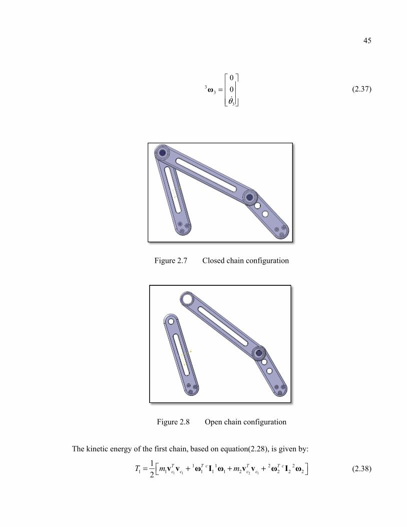
Figure 2.7 Closed chain configuration ........................................................................45
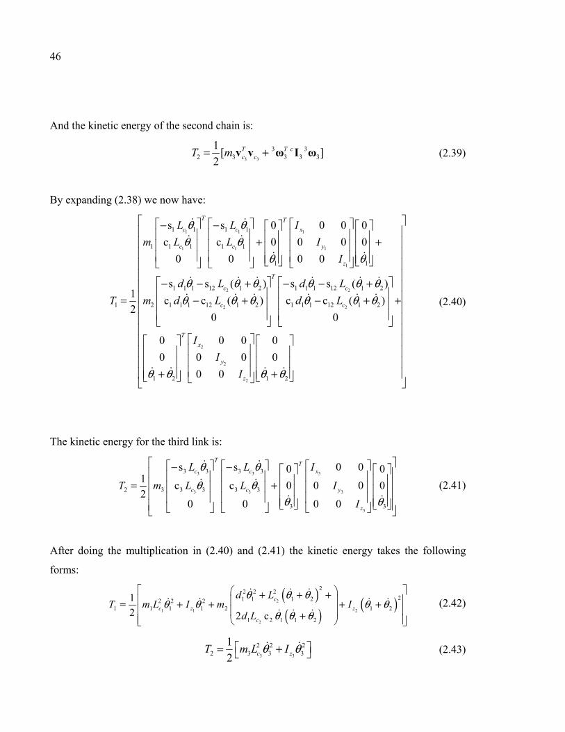
Figure 2.8 Open chain configuration ...........................................................................45
Figure 2.9 Desired trajectory for the angle of the first link of the robot .....................52
Figure 2.10 PD computed torque (top) and PID computed torque (bottom) ................55
Figure 2.11 Comparison of analytical and SimMechanics methods for the rigid model57
Figure 2.12 Comparison of the analytical and SimMechanics model by the difference of torques ...................................................................................................58
Figure 3.1 Robot composed of five subassemblies .....................................................59
Figure 3.2 Exploded view of parts for the third link subassembly ..............................61
Figure 3.3 Base subassembly as one rigid part ...........................................................62
Figure 3.4 Housing subassembly as one rigid part ......................................................62
Figure 3.5 Link one subassembly as one rigid part .....................................................63
1θ

XIV
Figure 3.6 Link two subassembly as one rigid part .....................................................63
Figure 3.7 Link three subassembly as one rigid part ...................................................64
Figure 3.8 Tools/Macro/Macros ..................................................................................65
Figure 3.9 Macros window ..........................................................................................66
Figure 3.10 Validation message ....................................................................................66
Figure 3.11 Feature selection for constraints ................................................................67
Figure 3.12 SimMechanics model of robot ...................................................................67
Figure 3.13 Simulink Library ........................................................................................68
Figure 3.14 Adding the number of actuators and sensors .............................................69
Figure 3.15 Selecting the actuation mode and its unit ..................................................69
Figure 3.16 Selecting measurement parameters and the units ......................................70
Figure 3.17 Position and velocity sensors .....................................................................70
Figure 3.18 Complete robot model ................................................................................71
Figure 4.1 P-type ILC block diagram ..........................................................................74
Figure 4.2 Combining ILC with computed torque ......................................................75
Figure 5.1 Simulation block diagram ..........................................................................77
Figure 5.2 Solver configurations .................................................................................77
Figure 5.3 Two successive cycles of trajectory of position, velocity and acceleration79
Figure 5.4 Required torque for the trajectory described in this section ......................80
Figure 5.5 Position error for computed torque controller ...........................................82
Figure 5.6 Position error for perturbed computed torque controller ...........................83
Figure 5.7 Position error for P-type ILC with ..............................................84
Figure 5.8 Position error for P-type ILC with ............................................85
Figure 5.9 RMS position error for P-type ILC with ...................................86
0.5pk =
0.05pk =
0.05pk =
XV
Figure 5.10 Maximum values of absolute error at each cycles .....................................87
Figure 5.11 Comparison between the error of the first and the last cycles for P-type ILC .............................................................................................................88
Figure 5.12 RMS position error for PD-type ILC with and ............89
Figure 5.13 Comparison between the error of the first and the last cycles for PD-type ILC .............................................................................................................90
Figure 5.14 Comparison of two types of ILC according to the RMS error convergence91
Figure 6.1 Actuator settings for obtaining the inverse dynamics model .....................94
Figure 6.2 Sensor settings for obtaining the inverse dynamics model ........................95
Figure 6.3 PID computed torque using inverse dynamic ............................................96
Figure 6.4 Configuring Simulink for TwinCAT file generation .................................96
Figure 6.5 Robot setup ..............................................................................................101
Figure 6.6 Position error for computed torque controller .........................................102
Figure 6.7 Position Error for P-type ILC with ...........................................103
Figure 6.8 RMS position error for P-type ILC with ...................................104
Figure 6.9 Position error for P-type ILC with ..........................................105
Figure 6.10 RMS position error for P-type ILC with .................................106
Figure 6.11 Maximum absolute error of position for P-type ILC with ......107
Figure 6.12 Comparison of error in first and last cycles for P-type ILC with 108
Figure 6.13 RMS position error for PD-type ILC with and ......109
Figure 6.14 Maximum absolute position error for PD-type ILC with and
..................................................................................................110
0.2pk = 0.2dk =
0.5pk =
0.5pk =
0.01pk =
0.01pk =
0.01pk =
0.01pk =
0.02pk = 0.02dk =
0.02pk =0.02dk =

XVI
Figure 6.15 Comparison of first and last cycles’ error for PD-type ILC with
and ...........................................................................................111
Figure 6.16 Comparison of the RMS of error convergence for the two types of ILC 112
0.02pk =0.02dk =
LIST OF ABBREVIATIONS 3D Three dimensions
CAD Computer aided design
CAE Computer aided engineering
CAM Computer aided manufacturing
ILC Iterative learning control
P Proportional
PD Proportional-derivative
PID Proportional-integral-derivative
TwinCAT The Windows Control and Automation Technology


LIST OF SYMBOLS AND UNITS OF MEASUREMENTS
First link length [m]
Second link length [m]
Third link length [m]
Distance between first link joint with ground and third link joint with ground
[m]
Angle between first link and horizontal line passing through two joints on
ground [rad]
Angle between first link and second link [rad]
Angle between third link and horizontal line passing through two joints on
ground [rad]
Angle between third link and second link [rad]
Torque produced in motor [N.m]
Derivation of with time [ ]
Derivation of with time [ ]
Derivation of with time [ ]
Derivation of with time [ ]
Power [Watt]
Motor shaft radius [m]
First link shaft radius connecting to ground [m]
First link mass [kg]
Second link mass [kg]
Third link mass [kg]
Kinetic energy [J]
1d
2d
3d
L
1θ
2θ
3θ
4θ
τ
1θ 1θ rad
s
2θ 2θ rad
s
3θ 3θ rad
s
1θ 1θ 2
rad
s
P
mr
1r
1m
2m
3m
T
XX
Potential energy [J]
Vector of non-conservative forces [N]
Distance between center of gravity of first link and joint of first link with
ground [m]
Distance between center of gravity of second link and the joint at either two
ends [m]
Distance between center of gravity of third link and joint of third link with
ground [m]
Position of center of gravity of link j in i coordinate [m]
Time [s]
First link desired angle [rad]
First link real angle [rad]
Velocity of first link center of gravity [ ]
Angular velocity of link j in i coordinate [ ]
Moment of inertia of link j at its center of gravity along perpendicular to
moving plane [ ]
Coriolis force matrix [N]
Mass matrix [kg]
Gear ratio
Total duration of trajectory from initial position to final position [s]
Initial position of first link [rad]
Final position of first link [rad]
Matrix of proportional gains for computed torque
dK Matrix of derivative gains for computed torque
iK Matrix of integral gains for computed torque
V
.n cQ
1cL
2cL
3cL
ijc
t
1 (t)dθ
1(t)θ
jcv m
s
ijω rad
s
cjΙ
2.kg m
F(θ,θ)
M(θ)
n
ft
0θ
fθ
pK

XXI
Derivative gain for ILC
Proportional gain for ILC
Integral gain for ILC
Response time [s]
Delay time [s]
dk
pk
ik
rT
dt


INTRODUCTION
The goal of virtual prototyping in mechanical design is to decrease the time and cost of
manufacturing. Computer aided design (CAD), computer aided manufacturing (CAM) and
computer aided engineering (CAE) are software that allow engineers to minimize the time
and cost of manufacturing. CATIA, one of the Dassault system productions, is a well-known
CAD/CAM/CAE software. However, unless a real model of the system is produced, or an
additional module is added to the software, engineers cannot observe all the facets and
defects of the system. To avoid all the defects with minimal time and cost, several
prototyping methods have been developed. In these methods engineers aim to detect the
problems of the system through testing the physical strength and geometrical limitations of
the model. Until now, the focus has been on the mechanical aspect of the system. The present
thesis will focus on the functionality of the system. In other words, our goal is to minimize
the cost and time of dynamic modeling and controller design. In robot modeling, it is difficult
to calculate the dynamics of the system with existing methods such as Lagrange or Newton-
Euler. With these methods, mistakes are often made. We will avoid this risk by using
CAD/CAM/CAE software to observe the dynamics of the system. Simulink is equipped with
lots of libraries including SimMechanics. In SimMechanics we can use geometrical
constraints to verify the behavior of the system in forward and inverse dynamics, so we no
longer need to use the time-consuming Lagrange and Newton-Euler methods.
However, this procedure is still complicated, and can be further simplified. Imagine we have
to design a robot containing hundreds of parts, including parallel or serial links, that works in
a 3D space. Even in SimMechanics, modeling hundreds of parts with geometrical and
mechanical constraints is not an easy task. We must also consider the task of manually
adding the inertial properties of these hundreds of parts in SimMechanics. So each software
has its own advantages and disadvantages: CATIA is extraordinary in 3D modeling but
unable to analyze the dynamic, whereas SimMechanics is perfect in dynamic analysis but not
user-friendly for 3D modeling. If only there were a way to use the benefits of each software
and avoid their drawbacks, then we could save lots of time and effort.
24
In a cooperative project with IREQ (Institut de recherche d’Hydro-Québec), we developed a
macro to convert CAD files from CATIA V6 to SimMechanics files, while respecting all the
geometrical and inertial properties of the system. In this thesis, the macro is validated
through a four bars parallel robot. We chose to use this simple robot, with just one degree of
freedom, for validation because the analytical model can be found manually. So the macro
will be validated by comparing the model obtained manually and the one obtained with the
macro. In order to validate the system in the context of prototyping, two control laws will be
generated using the macro: a computed torque position controller and an iterative learning
controller. The computed torque controller calculates the required torque for the actuator
based on the actual position and velocity of the robot and the desired acceleration. This
controller uses the inverse dynamics of the model to calculate the required torque.
What about the popular PID controller? While these controllers are effective and easy to
implement, they have some drawbacks which have caused engineers to turn to other kinds of
controllers. One of these flaws is the tracking error. After stability, the most critical factor in
control engineering is error. In industrial applications, most procedures are repeated through
different cycles, such as during pick-and-place tasks. Since one system is under operation
with similar trajectory and initial conditions, everything remains unchanged. In systems
controlled by PID controllers, the same error pattern will therefore emerge along the
trajectory in different cycles in the systems. However, iterative learning control (ILC) has the
potential to solve this problem. ILC, which was first introduced by Arimoto (1985), takes
advantage of the knowledge of error patterns to reduce the error in future cycles. We will use
this technique to train the system, so that knowledge of the results in the previous cycle will
be used to compensate for the error and converge it to near-zero.
The objective of this thesis is to provide a method of finding the dynamics of a mechanism
without involving the more complicated analytical methods. For our purposes, it suffices to
have the CAD model of the mechanism in CATIA V6. The dynamic model of a system
allows us to better design a controller such as computed torque. In order to reduce the

25
tracking error of the robot, which undergoes a repetitive procedure with identical conditions
at each iteration, we use ILC in a serial structure with the computed torque controller.
This work enabled users to save time when finding the dynamic model of a robot. It provides
an easy way to design a computed torque controller for the system, and shows how to reduce
the tracking error through the use of an ILC controller.
The first chapter presents a review of literature for robots, virtual prototyping, and ILC
controllers. Chapter Two concentrates on a four bars parallel robot. It explains the kinematic
and dynamic modeling of the robot, and discusses the method of trajectory planning and
computed torque design for this robot. Chapter Three presents a method of virtual
prototyping, and Chapter Four explains the different types of ILC. The simulation results are
presented in Chapter Five, and the experimental results in Chapter Six. Chapter Six also
contains some useful pieces of information about real robot set-up.


CHAPTER 1
REVIEW OF LITERATURE
1.1 Robots
A robot is a mechanical system that controls several degrees of freedom of the end-effector
(e.g., the hand of the robot) (Tsai, 1999). The links, all of which are rigid, are connected to
each other through revolute joints for rotation and prismatic joints for linear displacements.
Robots are classified into two main categories, according to the configurations of their
kinematic chains: serial robots and parallel robots.
1.1.1 Serial robots
Serial robots are made up of links that are attached in succession to each other by a one
degree of freedom joint (Tsai, 1999). This configuration makes an open kinematic chain.
Figure 1.1 shows an example of a serial robot. Serial robots typically experience problems
regarding the mass and inertia of new links when they are added to the previous links. The
actuators, from the end effector to the base, end up becoming larger and heavier. Their
additional mass results in augmentation of the position error from the base to the end effector
(Joubair, 2012).

28
Figure 1.1 An example of serial robot: the Scara Robot Taken from Merlet ((2006), p. 2)
1.1.2 Parallel robots
Usually, one can reduce the large mass and inertia of serial robot links by distributing the
load across several links, which are attached in a parallel configuration from the end effector
to the ground. In doing so, one creates a parallel robot, an example of which is shown in
Figure 1.2. A parallel manipulator is generally defined as a closed-loop kinematic chain
mechanism whose end-effector is linked to the base by several independent kinematic chains
(Merlet, 2006). Parallel robots are more rigid, due to their closed-loop mechanical structure.
Typically the actuators are attached to the base, enabling good precision since the mass of the
moving part is reduced (Joubair, 2012). Unlike with serial robots, however, not all the joints
of a parallel robot are actuated. While some of them are active (also known as actuated),
others are passive. Because of the geometrical constraints imposed by closed-loop
mechanical chains, the singularity problem is more likely to occur with parallel robots than
with serial ones.
29
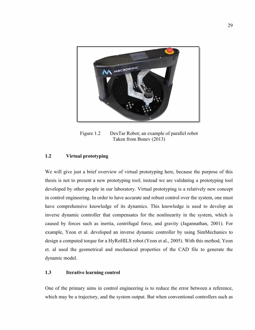
Figure 1.2 DexTar Robot; an example of parallel robot Taken from Bonev (2013)
1.2 Virtual prototyping
We will give just a brief overview of virtual prototyping here, because the purpose of this
thesis is not to present a new prototyping tool; instead we are validating a prototyping tool
developed by other people in our laboratory. Virtual prototyping is a relatively new concept
in control engineering. In order to have accurate and robust control over the system, one must
have comprehensive knowledge of its dynamics. This knowledge is used to develop an
inverse dynamic controller that compensates for the nonlinearity in the system, which is
caused by forces such as inertia, centrifugal force, and gravity (Jagannathan, 2001). For
example, Yeon et al. developed an inverse dynamic controller by using SimMechanics to
design a computed torque for a HyRoHILS robot (Yeon et al., 2005). With this method, Yeon
et. al used the geometrical and mechanical properties of the CAD file to generate the
dynamic model.
1.3 Iterative learning control
One of the primary aims in control engineering is to reduce the error between a reference,
which may be a trajectory, and the system output. But when conventional controllers such as

30
PID are combined with computed torque, and the trajectory is repetitive, the tracking error
typically does not change in different cycles.
In industry several processes are repetitive, particularly tasks accomplished by robots. The
process is repetitive when all the conditions are identically repeated in all cycles. For
example, a gripper picks up an object with mass m from point x1 and carries it through a
specific trajectory; it delivers the object to point x2 and then returns back to x1 to pick up the
next object with the same mass m. This would be one process. In the next cycle the robot
undergoes the same process and does the same duty. Under these conditions it is normal to
see the same error in each cycle of the process, since all the factors such as friction, dynamic
model, input, controller and trajectory are remaining constant.
If we can change the input of the system in a specific way so that the output will more
closely approach the desired trajectory, then we are successful in reducing the error. But what
is this specific way? This method is called Iterative Learning Control or ILC. An ILC block
diagram is shown in Figure 1.3.
With ILC, the robot tries to learn its error and correct its commands accordingly in order to
reduce the error in the next cycle. If we repeat this procedure several times, we expect that at
each cycle the error will be smaller than in the previous one, and so eventually the error will
converge to near-zero.
Figure 1.3 ILC block diagram

31
The output will be stored in memory in the -th cycle, and will be used during the ( )
-th cycle to change the input.
1.3.1 Iterative learning control definition
There are several definitions of ILC, but the following two descriptions represent the general
consensus:
• “The learning control concept stands for the repeatability of operating a given
objective system and the possibility of improving the control input on the basis of
previous actual operation data” (Arimoto, Kawamura and Miyazaki, 1986).
• ILC is a “recursive online control method that relies on less calculation and requires
less a priori knowledge about the system dynamics. The idea is to apply a simple
algorithm repetitively to an unknown plant, until perfect tracking is achieved” (Bien
and Huh, 1989).
1.3.2 Iterative learning control history
The idea of ILC was initially suggested in 1974 by (Edwards, 1974), with its first
formulation presented in Japan by Uchiyama in 1978 (Uchiyama, 1978). A learning
configuration is shown in Figure 1.4.
Figure 1.4 Learning control configuration
k 1k +

32
Later during 1980s, the idea was further developed by a group of researchers under
Arimoto’s supervision (1984). In the resulting article, Arimoto proposed this updating law:
(1.1)
The convergence is guaranteed according to the well-known small gain conditions. Here is
a constant matrix, which is the gain of the updating law. This algorithm is PD-type ILC
because it uses the derivative of the error. They also proposed other types of ILC (Arimoto,
1985), such as the following PID-type:
(1.2)
Togai and Yamano (1985) and Furuta and Yamakita (1987) focused on learning control for
discrete-time linear systems. So far, all the algorithms we have discussed used a unity
weighting on input. By contrast, Mita and Kato (1985) used separate weighting for the input
and error. Their updating law is:
(1.3)
Atkeson and McIntyre (1986) used the same approach to learning control as Arimoto et al.,
applied to linear robotic manipulator models. Hidge and Judd (1988) considered learning
control from a frequency domain point of view, which is similar to Mita and Kato’s work.
They also took the effect of disturbance into account, and applied it to the linear robotics
models. Oh, Bien and Suh (1988) proposed an approach to learning control for linear time
varying systems. Arimoto et al. (1984) also considered learning control for robotics, and
Craig (1984) and Gu and Loh (1989) suggested learning and adaptive control methods that
are similar to those of Arimoto. Harokopos (1986) worked on minimizing the functional cost
for robotics. Bondi, Casalino and Gambardella (1988) presented a high-gain feedback model
for learning control and applied it to nonlinear systems including manipulators. Yamakita
and Mita (1991) researched the domain of nonlinear systems through the use of Gateaux
derivatives. Messner, Horowitz, Kao and Boals (1991) developed a new method for
1k k ku u e+ = + Γ
Γ
1k k k k ku u e e e dt+ = + Φ + Γ + Ψ
1(s) ( )[ ( ) ( )]k k kU L s U s aE s+ = +
33
nonlinear manipulators. Hauser (1987) suggested the idea of using learning control to find
the inverse dynamics for nonlinear systems. Heinzinger, Fenwick, Paden, and Miyazaki
(1989) investigated the robustness of nonlinear systems in the ILC domain. Sugie and Ono
(1991) also worked on the robustness of iterative learning control. Lastly, (Ahn, Moore and
Chen, 2007) produced a survey of ILC research including journals articles and Ph.D.
dissertations from 1998 to 2004.
1.3.3 Assumptions used for ILC
As mentioned by Gauthier in his Ph.D. dissertation (Gauthier, 2008), the five key
assumptions used for ILC are:
• The initial state of the system remains identical throughout the process. Then,
and this initial condition gives the starting point of the desired
trajectory ;
• The system can be time-varying, but each cycle should be the same as the other
cycles. Then, for a system expressed in the state-space domain,
and ;
• The desired trajectory must be feasible. Then it should be
possible to have an input for such that the output follows the desired
trajectory. The input is a continuous function of time;
• should be unique to obtain the desired trajectory ;
• The cycle duration is similar from cycle to cycle (but there are some
exceptions)
All five of these assumptions are held throughout this thesis.
(0) (0),kx x k= ∀
(0) (0) (0),k k ky C x k= ∀
( ) ( ), ( ) ( ), ( ) ( ), [0, ]k k kA t A t B t B t C t C t t T= = = ∀ ∈ k∀
( ) (with [0, ])dy t t T∈
*( )u t [0, ]t T∈
2[0, ]L T
*( )u t (t)dy
T ∈

CHAPTER 2
ROBOT MODELING
2.1 Introduction
Parallel robots play an important role in industry. Their robustness, high speed capabilities,
and precision give them great advantages when it comes to certain manufacturing tasks.
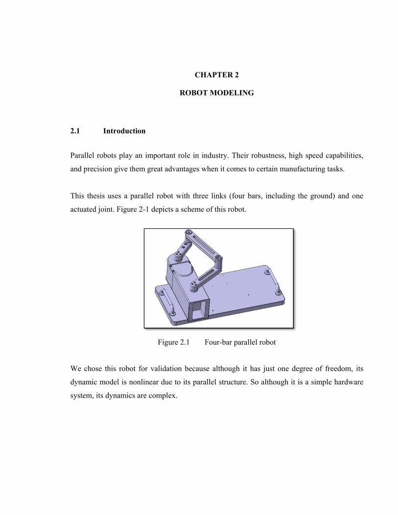
This thesis uses a parallel robot with three links (four bars, including the ground) and one
actuated joint. Figure 2-1 depicts a scheme of this robot.
Figure 2.1 Four-bar parallel robot
We chose this robot for validation because although it has just one degree of freedom, its
dynamic model is nonlinear due to its parallel structure. So although it is a simple hardware
system, its dynamics are complex.

36
2.2 Kinematic model
2.2.1 Direct kinematic
According to Figure 2-2, we find both and relative to , which is the input angle
(actuated joint). Figure 2-2 shows the geometric model of the robot links with their parameters.
Figure 2.2 Robot links with parameters
In this figure, l is the distance between the two joints attached on the base, d1 is the length of
the first link (the actuated link with motor), d2 is the length of the second link, d3 is the length
of the third link, is the angle between the first link and the line passing through two joints
on the ground, is the angle between the first and second link, is the angle between third
link and the line passing through the two joints on the ground, and is the angle between
the second and third link.
To find and relative to , we consider the links as vectors in two dimensional
Cartesian space. This consideration is shown in Figure 2.3.
2θ 3θ 1θ
1θ
2θ 3θ
4θ
2θ 3θ 1θ
37
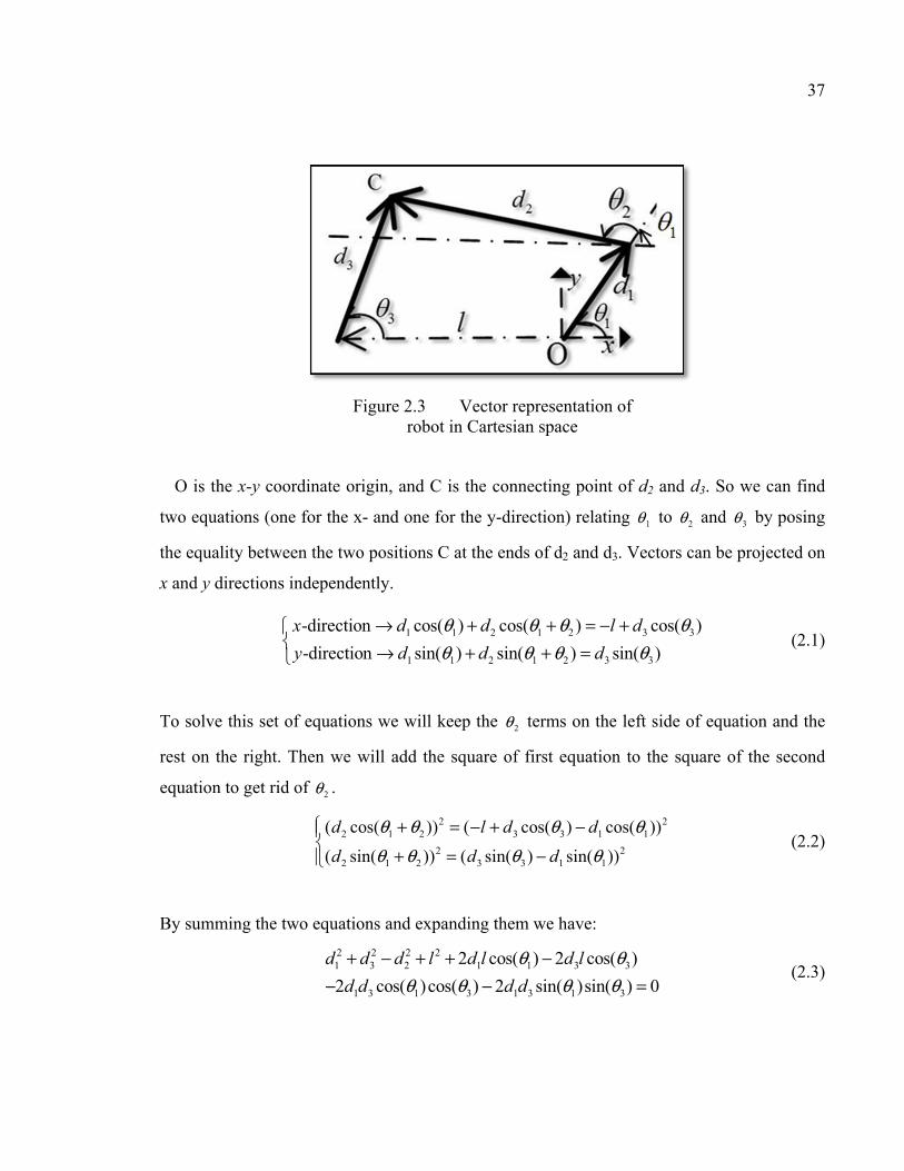
Figure 2.3 Vector representation of robot in Cartesian space
O is the x-y coordinate origin, and C is the connecting point of d2 and d3. So we can find
two equations (one for the x- and one for the y-direction) relating to and by posing
the equality between the two positions C at the ends of d2 and d3. Vectors can be projected on
x and y directions independently.
(2.1)
To solve this set of equations we will keep the terms on the left side of equation and the
rest on the right. Then we will add the square of first equation to the square of the second
equation to get rid of .
(2.2)
By summing the two equations and expanding them we have:
(2.3)
1θ 2θ 3θ
1 1 2 1 2 3 3
1 1 2 1 2 3 3
-direction cos( ) cos( ) cos( )
-direction sin( ) sin( ) sin( )
x d d l d
y d d d
θ θ θ θθ θ θ θ
→ + + = − + → + + =
2θ
2θ
2 22 1 2 3 3 1 1
2 22 1 2 3 3 1 1
( cos( )) ( cos( ) cos( ))
( sin( )) ( sin( ) sin( ))
d l d d
d d d
θ θ θ θθ θ θ θ
+ = − + −
+ = −
2 2 2 21 3 2 1 1 3 3
1 3 1 3 1 3 1 3
2 cos( ) 2 cos( )
2 cos( )cos( ) 2 sin( )sin( ) 0
d d d l d l d l
d d d d
θ θθ θ θ θ
+ − + + −− − =
38
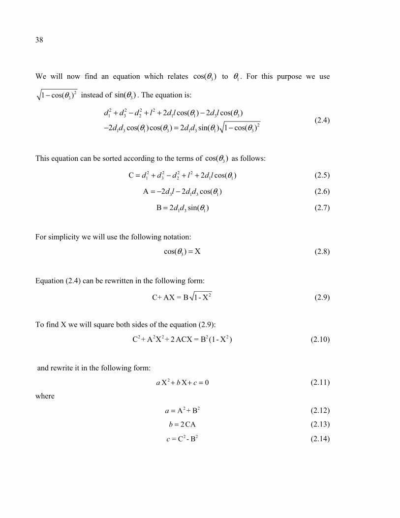
We will now find an equation which relates to . For this purpose we use
instead of . The equation is:
(2.4)
This equation can be sorted according to the terms of as follows:
(2.5)
3 1 3 12 2 cos( )d l d d θΑ = − − (2.6)
1 3 1B 2 sin( )d d θ= (2.7)
For simplicity we will use the following notation:
(2.8)
Equation (2.4) can be rewritten in the following form:
(2.9)
To find X we will square both sides of the equation (2.9):
2 2 2 2 2C + A X + 2 ACX = B (1- X ) (2.10)
and rewrite it in the following form:
(2.11)
where
(2.12)
(2.13)
(2.14)
3cos( )θ 1θ
231 cos( )θ− 3sin( )θ
2 2 2 21 3 2 1 1 3 3
21 3 1 3 1 3 1 3
2 cos( ) 2 cos( )
2 cos( )cos( ) 2 sin( ) 1 cos( )
d d d l d l d l
d d d d
θ θ
θ θ θ θ
+ − + + −
− = −
3cos( )θ2 2 2 21 3 2 1 1C 2 cos( )d d d l d l θ= + − + +
3cos( ) Xθ =
2C+ AX = B 1- X
2X X 0a b c+ + =
2 2A + Ba =
2CAb =2 2= C - Bc

39
Equation (2.11) is a simple second degree equation. To solve this equation we will calculate
the discriminant as follows:
(2.15)
And finally the answers to X (or ) are:
(2.16)
(2.17)
By solving these two equations we find the two possible answers for . So there are two
answers for angle , which corresponds to the positions of links 2 and 3 in up or down
positions, as shown in Figure 2.4.
Figure 2.4 Possible solutions for Position
up (left) – Position down (right)
The left configuration in Figure 2.4 is the current configuration of robot. Since the third link
does not go through a full rotation, due to the length of the link, the correct answer according
to our configuration choice is the one with between 0 and radians. Once we have found
, it is easy to find by using equation (2.1).
2 4b acΔ = −
3cos( )θ
3 1cos( )2
b
aθ − + Δ=
3 2cos( )2
b
aθ − − Δ=
3θ
1θ
1θ
3θ π
3θ 2θ

40
2.2.2 Singularities
For this robot, there are two positions in which we have serial singularities. Figure 2.5
presents these two singular positions, at and . The dimensions of the links are
chosen to avoid parallel singularities. There are two conditions to ensure this avoidance:
1 2 3
1 actuated link
d d d l
d
+ ≤ + →
where d1 is the length of the shortest link, which is equal to 68.58 mm. This link is actuated.
d2 is the length of the longest link, which is equal to 149.225 mm. The lengths of the two
remaining links are denoted by d3 and l, respectively, with l equal to 149.225 mm and d3
equal to 114.30 mm. In this robot design, these two conditions are respected.
Figure 2.5 Two serial singularities
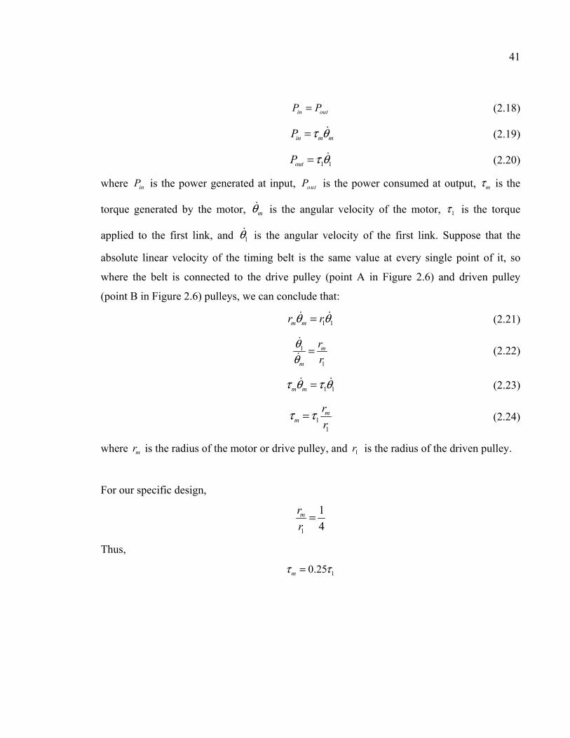
2.3 Dynamic model
For the dynamic model we will consider that the motor is directly mounted on the first link
and we will neglect any flexibility. In this section, the matrix of mass and vector of nonlinear
forces will be derived according to the Lagrange method (Craig, 2005). This is done in order
to compute the necessary torque for the motor to follow a desired trajectory. The ratio of the
driven pulley to the drive pulley is 4:1, meaning the angular velocity of the drive pulley is
four times greater than the angular velocity of the driven pulley. It is also known that (when
the mechanical loss is ignored) the power generated by the motor is equal to the power
consumed by the robot, as described by the following:
2 0θ = 2θ π=
68.58 149.225 149.225 114.30+ ≤ +
41
(2.18)
(2.19)
(2.20)
where is the power generated at input, is the power consumed at output, is the
torque generated by the motor, is the angular velocity of the motor, is the torque
applied to the first link, and is the angular velocity of the first link. Suppose that the
absolute linear velocity of the timing belt is the same value at every single point of it, so
where the belt is connected to the drive pulley (point A in Figure 2.6) and driven pulley
(point B in Figure 2.6) pulleys, we can conclude that:
(2.21)
(2.22)
(2.23)
(2.24)
where is the radius of the motor or drive pulley, and is the radius of the driven pulley.
For our specific design,
Thus,
in outP P=
in m mP τ θ=
1 1outP τ θ=
inP outP mτ
mθ 1τ
1θ
1 1m mr rθ θ=
1
1
m
m
r
r
θθ
=
1 1m mτ θ τ θ=
11
mm
r
rτ τ=
mr 1r
1
1
4mr
r=
10.25mτ τ=
42
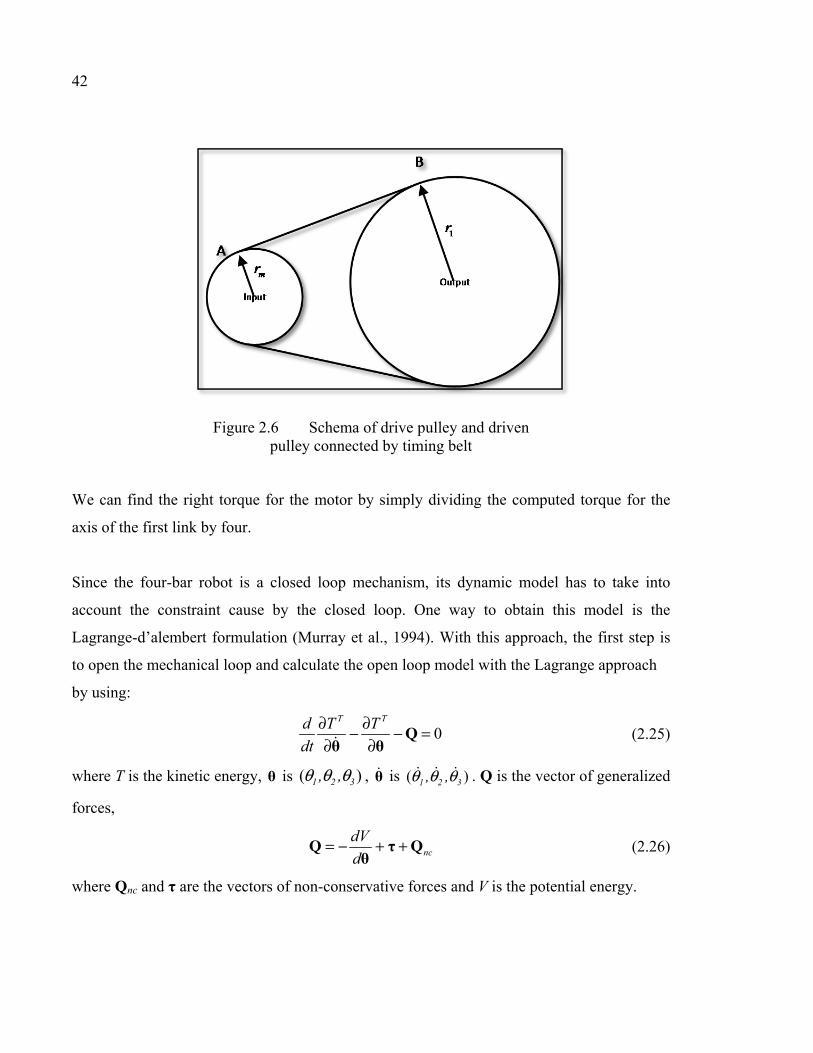
Figure 2.6 Schema of drive pulley and driven pulley connected by timing belt
We can find the right torque for the motor by simply dividing the computed torque for the
axis of the first link by four.
Since the four-bar robot is a closed loop mechanism, its dynamic model has to take into
account the constraint cause by the closed loop. One way to obtain this model is the
Lagrange-d’alembert formulation (Murray et al., 1994). With this approach, the first step is
to open the mechanical loop and calculate the open loop model with the Lagrange approach
by using:
(2.25)
where T is the kinetic energy, is , is . Q is the vector of generalized
forces,
(2.26)
where Qnc and τ are the vectors of non-conservative forces and V is the potential energy.
0T Td T T
dt
∂ ∂− − =∂ ∂
Qθ θ
θ ( )1 2 3, ,θ θ θ θ ( )1 2 3, ,θ θ θ
nc
dV
d= − + +Q τ Q
θ

43
As shown in Figures 2-7 and 2-8, we chose to open the loop at point C. For the open loop
configuration, we thus consider link one and two as the first chain and link three as the
second chain.
Since all arms are moving in a plane perpendicular to the direction of gravity, the potential
energy is constant and the variation is zero:
(2.27)
Then, the kinematic energy of the 3 links in the open loop configuration is:
(2.28)
where is the velocity of the center of gravity of link I, is the moment of
inertia of link i about its center of gravity, and is the angular velocity of link i. To find
the velocity of the center of gravity, we will first find the position of this point, and then we
will derivate it. The position of the first link’s center of gravity is:
(2.29)
where is the center of gravity of the first link, is the position of the center of gravity
of link j at the i coordinate, is , and is . Derivation of (2.29) gives the
velocity of the center of gravity of the first link. The velocity of the first link’s center of
gravity, , is:
(2.30)
The angular velocity of the first link is:
0dV =
3
1
1
2 i i
T i T c ii c c i i i
i
T m=
= + v v ω I ω
3
jc ∈v 3 3ci
×∈I
iiω
1
1
10
1 1
c
s
0
c
c
L
L
=
c
1cL ijc
1c 1cos( )θ 1s 1sin( )θ
1cv
1
1 1
1 1
1 1
0
c
c c
s L
c L
θθ
− =
v

44
(2.31)
where is the angular velocity of link j projected in i coordinate. The velocity of the
center of gravity of the second link is calculated similarly to the first link. First, the position
of this point must be found. It is:
(2.32)
where is , and is . Then the derivative of (2.32) gives the
velocity of the center of gravity of the second link:
(2.33)
The angular velocity for the second link is:
(2.34)
Just like before, we will find the position of the center of mass of the third link:
(2.35)
Consequently the velocity of this point is:
(2.36)
And the angular velocity of the third link is:
11
1
0
0
θ
=
ω
3ij ∈ω
2
2
1 1 120
2 1 1 12
c c
s s
0
c
c
d L
d L
+ = +
c
12s 1 2sin( )θ θ+ 12c 1 2cos( )θ θ+
2
2 2
1 1 1 12 1 2
1 1 1 12 1 2
s s ( )
c c ( )
0
c
c c
d L
d L
θ θ θθ θ θ
− − + = − +
v
22
1 2
0
0
θ θ
=
+
ω
1
1
10
3 1
c
s
0
c
c
L l
L
− =
c
3
3 3
3 3
3 3
s
c
0
c
c c
L
L
θθ
−
=
v
45
(2.37)
Figure 2.7 Closed chain configuration
Figure 2.8 Open chain configuration
The kinetic energy of the first chain, based on equation(2.28), is given by:
(2.38)
33
3
0
0
θ
=
ω
1 1 2 1
1 1 2 21 1 1 1 1 2 2 2 2
1
2T T c T T cc c c cT m m = + + + v v ω I ω v v ω I ω
46
And the kinetic energy of the second chain is:
(2.39)
By expanding (2.38) we now have:
(2.40)
The kinetic energy for the third link is:
(2.41)
After doing the multiplication in (2.40) and (2.41) the kinetic energy takes the following
forms:
(2.42)
(2.43)
3 3
3 32 3 3 3 3
1[ ]
2T T cc cT m= +v v ω I ω
1 1 1
1 1 1
1
2 2
2
1 1 1 1
1 1 1 1 1
1 1
1 1 1 12 1 2 1 1 1 12
1 2 1 1 1 12 1 2
s s 0 0 0 0
c c 0 0 0 0
0 0 0 0
s s ( ) s s (1
c c ( )2
0
T T
c c x
c c y
z
T
c c
c
L L I
m L L I
I
d L d L
T m d L
θ θθ θ
θ θ
θ θ θ θθ θ θ
− − + +
− − + − − = − +
2
2
2
2
1 2
1 1 1 12 1 2
1 2 1 2
)
c c ( )
0
0 0 0 0
0 0 0 0
0 0
c
T
x
y
z
d L
I
I
I
θ θθ θ θ
θ θ θ θ
+ − + +
+ +
3 3 3
3 3 3
3
3 3 3 3
2 3 3 3 3 3
3 3
s s 0 00 01
c c 0 0 0 02
0 0 0 0
TT
c c x
c c y
z
L L I
T m L L I
I
θ θθ θ
θ θ
− − = +
( )( )
( )2
1 1 2
2
22 2 221 1 1 22 2 2
1 1 1 1 2 1 2
1 2 1 1 2
1
2 2 c
c
c z z
c
d LT m L I m I
d L
θ θ θθ θ θ θ
θ θ θ
+ + + = + + + + +
3 3
2 2 22 3 3 3
1
2 c zT m L Iθ θ = +
47
In order to find the equation of motion from kinetic energy we must do some derivations, as
explained in (2.25):
(2.44)
Note that by we mean that should be partially derived with respect to and
respectively.
The time derivative of equation (2.44) is:
(2.45)
The partial derivative of kinetic energy based on is:
(2.46)
(2.47)
( )( ) ( )
( )( ) ( )
2
1 1 2
2
2 2 2
3 3
2 21 1 1 1 22
1 1 1 2 1 2111 2 1 2
1,2 12
2 1 2 1 1 1 22
223 3 3
3
c 2
T
cT c z z
cT
c c z
T
c z
T d Lm L I m IT d L
Tm L d L I
Tm L I
θ θ θθ θ θ θθ θ θ
θθ θ θ θ θθ
θ θθ
∂ + + + + + + +∂∂ += = ∂ ∂ + + + +∂
∂ = + ∂
1,2
TT
θ∂∂
TT 1θ 2θ
( )( )( )
( )
( )( ) ( )
2
1 1 2 2
2
2 2 2 2
2 21 1 1 2
21 1 1 2 1 2 2 1 2 1 2
1
1,2 1 2 2 1 2
22 1 2 1 2 1 2 1 2 1 1 2
2
s 2
c 2
s c
c
T c z c z
c
c c c z
T
d L
m L I m d L Id T
dt d L
m L d L d L I
d T
dt
θ θ θ
θ θ θ θ θ θ θ
θ θ θ θ
θ θ θ θ θ θ θ
+ + − + + + + + +∂ = ∂ + + − + + +
∂
3 3
23 3 3
3c zm L Iθ θ
θ = + ∂
θ
( )2
1
11
2 1 2 1 1 21,2 1
2
0
s
T
T
Tc
dT
dTm d LdT
d
θθ θ θθ
θ
∂ = = − +∂
[ ]2
3
0TT
θ∂ =∂

48
(2.48)
And the vector of generalized forces is:
where is the vector of the applied torque to the joints, is the vector of the non-
conservative forces like friction or external forces which in this case will be ignored, and V is
the potential energy. As mentioned before, the differentiation in potential energy in this robot
is zero since there is no elevation differentiation in robot arms.
Thus,
By taking the derivations and doing the simplification, the following equation is achieved:
(2.49)
where and .
This equation can be written in the following form:
(2.50)
where is the mass matrix, and is the matrix of the Coriolis force.
0T Td T T
dt
∂ ∂− − =∂ ∂
Qθ θ
nc
dV
d= − +Q τ+ Q
θ
τ ncQ
0
0
τ =
Q
( )( )( )
( )
( )( ) ( )
2
1 1 2 2
2
2 2 2 2
3
2 21 1 1 2
21 1 1 2 1 2 2 1 2 1 2
1
1 2 2 1 2
22 1 2 1 2 1 1 2 1 1 2
23 3
s 2 0
0c 2
s c
c
c z c z
c
c c c z
c
d L
m L I m d L I
d L
m L d L d L I
m L I
θ θ θ
θ θ θ θ θ θ θ
θ θ θ
θ θ θ θ θ θ
θ
+ + − + + + + + + − = + + − + + +
+
Q
[ ]3 3 2 0z θ − = Q
1 0
τ =
Q [ ]2 0=Q
( ) ( ), τM θ θ+ F θ θ = β
( ) 3 3×∈M θ ( ) 3∈F θ,θ
49
The mass matrix is:
(2.51)
The Coriolis force matrix is:
(2.52)
And β is the coupling matrix:
(2.53)
Up to now, we have not considered the constraints. The second step is to close the
mechanical loop by taking into account the kinematic constraint given by equation (2.1). The
constraint in x direction is gx:
(2.54)
And the constraint in y direction is gy:
(2.55)
Thus, g is the vector of constraints:
(2.56)
By differentiating this constraint relative to time, we can write:
( ) 2 2
1 2
2 2
2 2 2 2
3
1
3
2 2 22 1
1 1 2 2
1 2 1 2
2 22 1 2 2
2
2
3
( ) ( )
2 ( ) ( )
(( )
0
0
0 0
( ) ) ( )
( )
c c
c z
c
z
c
c c z c z
c
d L Lm L Ic m I m I
d L c d L c
m L d L c I m L I
I m L
c + + +
+ + + +
+ + +
=
+
M
( )2
2
2 1 2 2 1 2
22 1 2 1
2
0
c
c
m d L s
m d L s
θ θ θ
θ
− +
=
F
[ ]T1 0 0=β
1 1 2 1 2 3 3= cos( ) cos( ) - cos( ) - 0xg d d d lθ θ θ θ+ + =
1 1 2 1 2 3 3sin( ) sin( ) -d sin( ) 0yg d dθ θ θ θ= + + =
x
y
g
g
=
g

50
(2.57)
where the Jacobian matrix of the constraint g is given by:
(2.58)
After doing all the partial derivatives in(2.58), the following Jacobian is derived:
(2.59)
where is , is , is , and is . It is possible to
separate the Jacobian into two parts:
(2.60)
where is associated with coordinate 1, and is associated with the two other
coordinates, namely 2 and 3. According to (Murray et al., 1994) the constraint can be
incorporated into the model by using the Lagrange-d’Alembert formulation. Equation (2.50)
can be reduced to the following form:
1 1 1 1( ) ( , ) τ+ =M θ θ F θ θ β (2.61)
where
(2.62)
(2.63)
(2.64)
0=gJ θ
1 2 3
1 2 3
x x x
y y y
g g g
g g g
θ θ θ
θ θ θ
∂ ∂ ∂ ∂ ∂ ∂ =∂ ∂ ∂ ∂ ∂ ∂
gJ
2 12 1 1 2 12 3 3
2 12 1 1 2 12 3 3
s s s s
c c c c
d d d d
d d d d
− − − = + −
gJ
12s 1 2sin( )θ θ+ 12c 1 2cos( )θ θ+ 3s 3sin( )θ 3c 3cos( )θ
1
2
2 12 1 1
2 12 1 1
2 12 3 3
2 12 3 3
s s
c c
s s
c c
d d
d d
d d
d d
− − = +
− = −
g
g
J
J
1gJ2gJ
1 2
2 1
11( ) ( )T Tg g
g g
−−
= − −
IM θ I J J M θ
J J
1 2
2 1
1 1 1
0( ) ( ) ( )
( )T Tg g
g g
d
dt
−−
= − + − −
F θ,θ I J J F θ,θ M θ θJ J
1 21T Tg g
− = − β I J J β

51
Equation (2.61) is the final dynamic equation.
2.4 Trajectory
To validate the controllers that will be implemented on the four-bar prototype, we choose a
seventh degree polynomial trajectory:
(2.65)
(2.66)
(2.67)
(2.68)
To ensure the smooth start and stop of the trajectory, the velocity, acceleration, and
derivative of the acceleration (jerk) should be zero in the initial and final positions. By
solving (2.65), (2.66), (2.67) and (2.68) together for the initial and final conditions, and
knowing that the position at is , and at is , the parameters will be
determined with the knowledge that is the destination point, and is the desired velocity
with which we want the link to go from the initial position to the final one.
In order to respect these conditions, the parameters of the trajectory can be chosen as:
(2.69)
(2.70)
(2.71)
(2.72)
(2.73)
2 3 4 5 6 71 0 1 2 3 4 5 6 7a a t a t a t a t a t a t a tθ = + + + + + + +
2 3 4 5 61 1 2 3 4 5 6 72 3 4 5 6 7a a t a t a t a t a t a tθ = + + + + + +
2 3 4 51 2 3 4 5 6 72 6 12 20 30 42a a t a t a t a t a tθ = + + + + +
2 3 41 3 4 5 6 76 24 60 120 210a a t a t a t a tθ = + + + +
0 0t = 0θ 0fft
θ θθ−
= fθ
fθ θ
0 0a θ=
1 2 3 0a a a= = =
3 30
4 7
35( )f f ft ta
tf
θ θ− −=
5 50
5 10
1008( 1008 )
12f f ft t
atf
θ θ−=
06 6
70( )fatf
θ θ− −=

52
(2.74)
For our validation, the desired starting point of the first link is zero radian, and it has to reach
radians in 0.5 seconds . The corresponding trajectory is shown in Figure 2-9.
Figure 2.9 Desired trajectory for the angle of the first link of the robot
2.5 Command law
In this section, we use the mass matrix and Coriolis-force matrix determined in the previous
section to present the computed torque that is used to control the angle of the first link of the
robot.
2.5.1 Computed torque
The knowledge of the dynamic model of the robot enables the design of precise and energy-
efficient controllers such as computed torque. This model base controller allows the robot to
07 7
20( )fatf
θ θ−=
π
53
follow the desired trajectory very quickly and with a small error. The more precise the
model, the smaller the error will be. Another name for “computed torque” is “linearizing
controller,” since if we consider the dynamic model of the robot:
(2.75)
Here , , and denotes the real angular position, real angular velocity, and real angular
acceleration of the robot joints, so the linearizing control law will be:
(2.76)
All the terms cancel out and the linear system is now:
(2.77)
(2.78)
where and are the matrices of derivative and proportional gains.
If the matrices of and are diagonal, then the dynamic of error is:
(2.79)
For all the actuated links we have:
0i ii d i p ie K e K e+ + = (2.80)
where [1, n]i = .
The gains can be calculated in order to impose the poles of the characteristic equation. For
example, the following gains will generate a zero overshoot with response time of :
(2.81)
(2.82)
where is a pole of multiplicity two given by:
(2.83)
The linearization controller of (2.74) can also be combined with a PID:
(2.84)
( ) ( )+ =M θ θ F θ,θ τ
θ θ θ
( ) ( )=τ M θ u + F θ,θ
θ= u
d d d p du = θ + K (θ -θ) + K (θ -θ)
dK pK
dK pK
( )d d d p d−θ θ + K (θ -θ) + K (θ -θ) = 0
rT
2p λ=K I
2d λ=K I
λ
4.73
rTλ =
( ) ( ) ( )d d d p d i d dt= + − + − + −u θ K θ θ K θ θ K θ θ
54
where is the matrix of integral gain.
If the matrices of , and are diagonal, then the dynamic of error is:
(2.85)
Again the gains can be calculated in order to impose the poles of characteristic equation. For
example the following gains will generate a zero overshoot with response time of :
(2.86)
(2.87)
(2.88)
where is a pole of multiplicity three given by:
(2.89)
The PD computed torque and PID computed torque are illustrated in Figure 2-10.
iK
dK pK iK
( ) ( ) ( ) ( ) 0d d d p d i d dt− + − + − + − =θ θ K θ θ K θ θ K θ θ
rT
23p λ=K I
3i λ=K I
3d λ=K I
λ
6.27
rTλ =

55
Figure 2.10 PD computed torque (top) and PID computed torque (bottom)
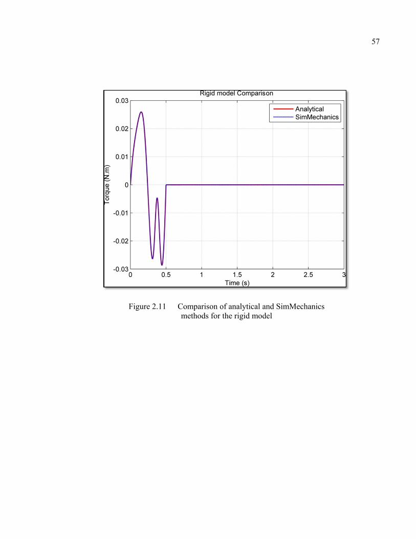
2.6 Validation of the model
For validation, the robot is modeled manually in SimMechanics according to the table of
mechanical properties shown in Table 2.1. For this purpose we used the inverse of the
dynamic model in SimMechanics as the computed torque controller. The next step is to
compare, for the same trajectory, the torques generated by the SimMechanics method with
those generated by the analytical method. If the torques are similar then the results validate

56
our analytical model. The comparison of torques for the SimMechanics method and the
analytical method can be found in Figures 2-11 and 2-12.
Table 2.1 Mechanical parameters of the four-bar robot
Parameters Variables Values Units
First link length
Second link length
Third link length
Distance between two joints attached to
ground
First link center of gravity1
Second link center of gravity
Third link center of gravity1
First link mass
Second link mass
Third link mass
First link moment of inertia2
Second link moment of inertia2
Third link moment of inertia2
Pulleys speed reduction ratio -
1 The center of gravity is measured from the joint attached to the ground. 2 The moment of inertia is about the z-axis parallel to the gravity direction. It is measured about the center of gravity.
1d 68.58 mm
2d 149.225 mm
3d 114.3 mm
l 149.225 mm
1cL 29.748 mm
2cL 149.225 74.61252 = mm
3cL 53.54 mm
1m 0.088 kg
2m 0.166 kg
3m 0.138 kg
1c I 56 .449 10 −× 2.kg m
2c I 44.63 10−× 2.kg m
3c I 42.265 10 −× 2.kg m
n 1 : 4
57
Figure 2.11 Comparison of analytical and SimMechanics methods for the rigid model
58
Figure 2.12 Comparison of the analytical and SimMechanics model by the difference of torques
Figure 2.11 shows that the two models are very similar. Figure 2.12 represents the difference
between the torque of the analytical model and the torque of the SimMechanics model. The
order of difference shows that the two models act very similarly for the same trajectory.
Consequently we can conclude that our analytical model is accurate.
CHAPTER 3
VIRTUAL PROTOTYPING
The aim of virtual prototyping is to save time in modeling the dynamics of a system without
involving the complicated equations. For this purpose we need to use the related software.
3.1 Modeling the robot in CATIA V6
To validate the virtual prototyping we modeled the four-bar mechanism in CATIA V6 with
all of the detailed parts. The proper materials were selected for the links and other parts. This
allows the software to determine the mechanical properties, such as mass and moment of
inertia, for each part. By modeling the parts geometrically, the software is also able to
determine the center of gravity and inertia. So far the mechanical properties of the system are
known by the software. We need only to impose the mechanical constraints on the system.
The mechanical constraints are applied to the parts to form the final product, as shown in
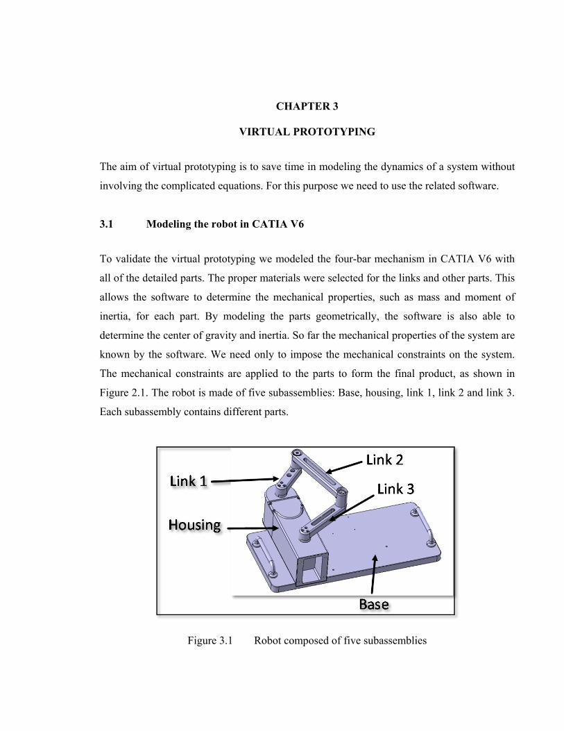
Figure 2.1. The robot is made of five subassemblies: Base, housing, link 1, link 2 and link 3.
Each subassembly contains different parts.
Figure 3.1 Robot composed of five subassemblies

60
The macro, which was developed by members of our research laboratory (The CORO Lab)
and is explained in the next section, considers only the constraints between subassemblies. It
does not matter which kind of constraint is used inside the subassemblies between parts,
because the macro treats each subassembly (with its distinct parts) as a rigid body. We will
model the robot so that the collection of all moving objects that are immobile relative to each
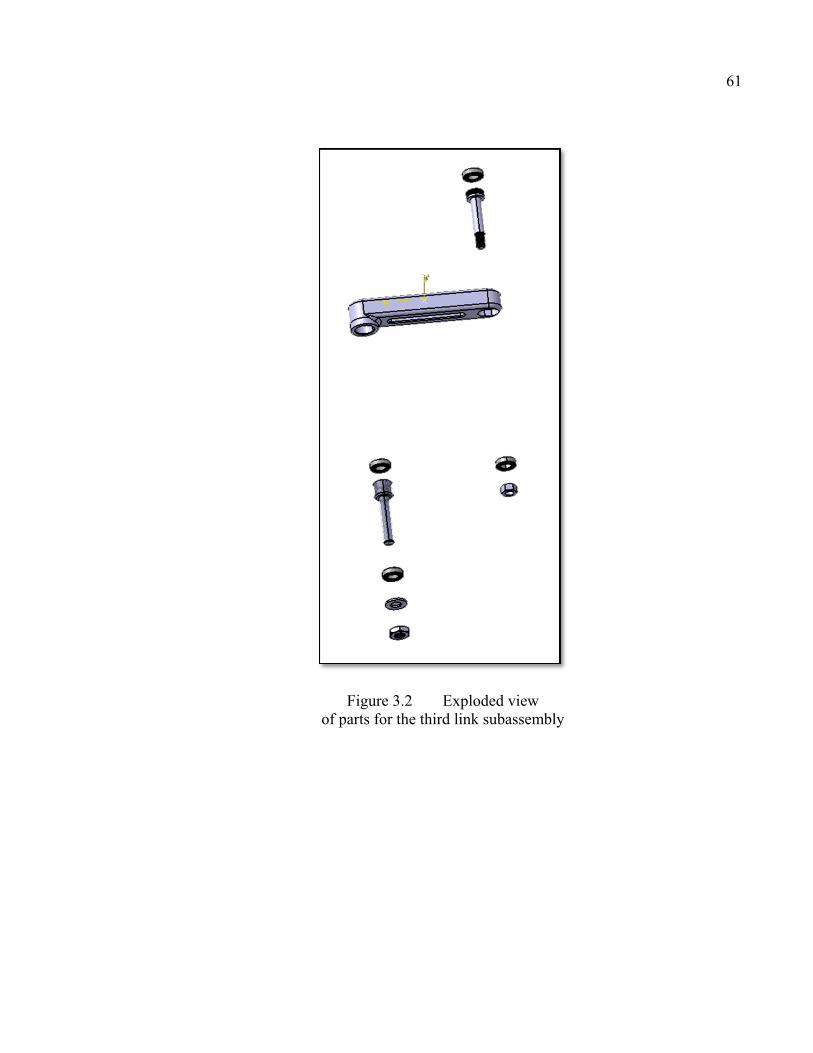
other is considered a subassembly. For example, in Figure 3.2 all the parts are moving, but
they are immobile relative to each other, and thus they form one subassembly. To simplify
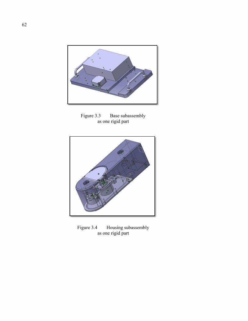
the model we divided the ground into two subassemblies, base and housing, which are
connected to each other with a fixed constraint. The complete list of subassemblies is: base,
housing, first link, second link and third link. The base and housing are connected to each
other with a fixed joint (welding joint) and the other subassemblies are connected by revolute
joints.
61
Figure 3.2 Exploded view of parts for the third link subassembly
62
Figure 3.3 Base subassembly as one rigid part
Figure 3.4 Housing subassembly as one rigid part
63
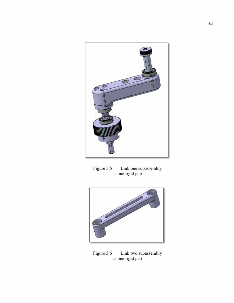
Figure 3.5 Link one subassembly as one rigid part
Figure 3.6 Link two subassembly as one rigid part
64
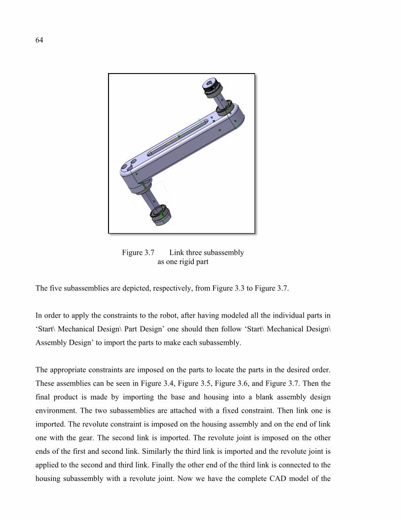
Figure 3.7 Link three subassembly as one rigid part
The five subassemblies are depicted, respectively, from Figure 3.3 to Figure 3.7.
In order to apply the constraints to the robot, after having modeled all the individual parts in
‘Start\ Mechanical Design\ Part Design’ one should then follow ‘Start\ Mechanical Design\
Assembly Design’ to import the parts to make each subassembly.
The appropriate constraints are imposed on the parts to locate the parts in the desired order.
These assemblies can be seen in Figure 3.4, Figure 3.5, Figure 3.6, and Figure 3.7. Then the
final product is made by importing the base and housing into a blank assembly design
environment. The two subassemblies are attached with a fixed constraint. Then link one is
imported. The revolute constraint is imposed on the housing assembly and on the end of link
one with the gear. The second link is imported. The revolute joint is imposed on the other
ends of the first and second link. Similarly the third link is imported and the revolute joint is
applied to the second and third link. Finally the other end of the third link is connected to the
housing subassembly with a revolute joint. Now we have the complete CAD model of the
65
robot with all its mechanical and geometrical properties. We just need a program to access
these properties.
3.2 Develop a macro
Another member of our team has developed a macro to extract the geometric and dynamic
information from the CAD model. To use this macro, the subassemblies should be connected
together with either fixed, revolute, or prismatic joints. For the present robot we used only
fixed and revolute joints to connect the subassemblies together.
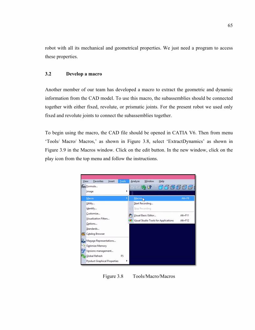
To begin using the macro, the CAD file should be opened in CATIA V6. Then from menu
‘Tools/ Macro/ Macros,’ as shown in Figure 3.8, select ‘ExtractDynamics’ as shown in
Figure 3.9 in the Macros window. Click on the edit button. In the new window, click on the
play icon from the top menu and follow the instructions.
Figure 3.8 Tools/Macro/Macros

66
Figure 3.9 Macros window
The macro will detect the five subassemblies and their constraints, as shown in Figure 3.10.
Figure 3.10 Validation message
We then select the features that define each constraint. For example, the revolute joint
between links three and two is on a bolt on the third link and a hole on the second link. So we
should select the hole and the bolt as the features for the connection. Figure 3.11 shows the
procedure of selecting the feature for the constraint between link two and link three.

67
Figure 3.11 Feature selection for constraints
This procedure should be done for all of the connections. At the end, the macro will generate
the XML file that should be saved on the computer. This file includes all geometric
properties for each subassembly, their respective centers of gravity, and the inertial
parameters, such as mass and moment of inertia. The file connects all of them with the proper
constraints.
3.3 Adding sensors and actuators in SimMechanics
The XML generated by the CATIA MACRO file should be copied in the Matlab current
folder. Using the command ‘mech_import filename.xml’ in the Matlab workspace will
generate a model for SimMechanics. See Figure 3-11 for an example.
Figure 3.12 SimMechanics model of robot
Since CATIA does not involve the movement of the mechanism, the generated model does
not have an actuator and sensor. However, we can manually add the sensor and actuator from
68
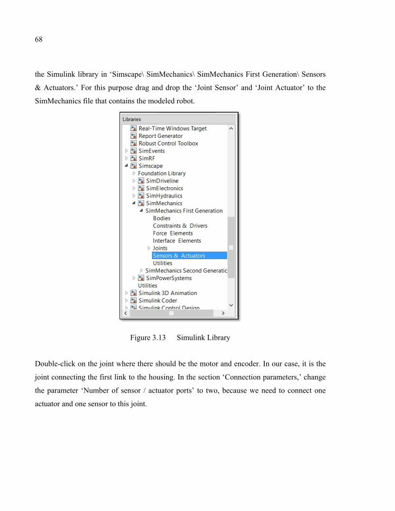
the Simulink library in ‘Simscape\ SimMechanics\ SimMechanics First Generation\ Sensors
& Actuators.’ For this purpose drag and drop the ‘Joint Sensor’ and ‘Joint Actuator’ to the
SimMechanics file that contains the modeled robot.
Figure 3.13 Simulink Library
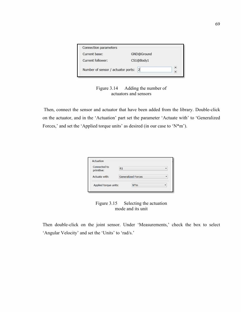
Double-click on the joint where there should be the motor and encoder. In our case, it is the
joint connecting the first link to the housing. In the section ‘Connection parameters,’ change
the parameter ‘Number of sensor / actuator ports’ to two, because we need to connect one
actuator and one sensor to this joint.
69
Figure 3.14 Adding the number of actuators and sensors
Then, connect the sensor and actuator that have been added from the library. Double-click
on the actuator, and in the ‘Actuation’ part set the parameter ‘Actuate with’ to ‘Generalized
Forces,’ and set the ‘Applied torque units’ as desired (in our case to ‘N*m’).
Figure 3.15 Selecting the actuation mode and its unit
Then double-click on the joint sensor. Under ‘Measurements,’ check the box to select
‘Angular Velocity’ and set the ‘Units’ to ‘rad/s.’

70
Figure 3.16 Selecting measurement parameters and the units
If angular velocity has been chosen, we could add an integral block from the Simulink library
to calculate the position (in our case, the position of the first link). In that case, discontinuity
will be avoided at each 2π rad position.
Figure 3.17 Position and velocity sensors
Finally the robot model can be completed with one input for torque and two outputs for
position and velocity.
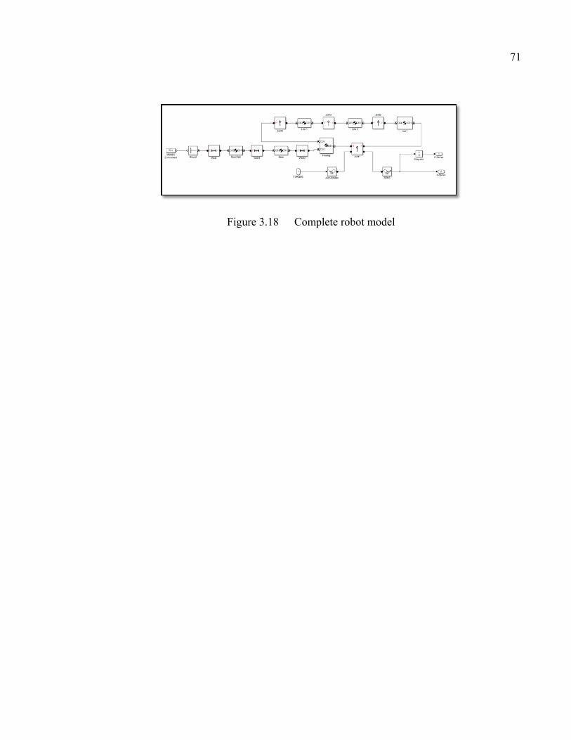
71
Figure 3.18 Complete robot model


CHAPTER 4
ITERATIVE LEARNING CONTROL
4.1 ILC algorithms
In this chapter, we will explore different approaches to iterative learning control (ILC), and
then two types of ILC will be used to validate the macro that was presented in Chapter Three.
As discussed previously, in repetitive processes with identical conditions in each cycle, the
error remains unchanged throughout the process. One way to decrease the error over time is
with ILC. For the cycle-to-cycle processes which each cycle is exactly the same as the next
one, it is possible to benefit from this method of control.
The term “iterative learning control” was first introduced by Arimoto (Moore, 1993). ILC is
a way to improve the transient response performance of systems that operate repetitively over
a fixed time interval (Moore, 1993). The idea of iterative learning control is to modify the
input of the system by training the system in such a way as to converge yk (output) as closely
as possible to yd (desired periodic trajectory) – put simply, to minimize the error (Moore,
1993). Generally speaking, there are two types of ILC updating law: P-type and PD-type
(Yang Quan and Moore, 2002). We will study P-type and PD-type ILC as applied to the
parallel robot described in previous chapters.
4.1.1 P-type ILC
The most basic ILC algorithm is the P-type ILC. The following formula is used to obtain the
input at time t inside the k+1 -th cycle:
(4.1)
where the error is:
(4.2)
1( )ku t+
1( ) ( ) ( )k k p ku t u t k e t+ = +
( )ke t
( ) ( ) ( )k d ke t y t y t= −
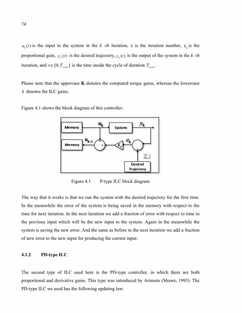
74
is the input to the system in the k -th iteration, is the iteration number, is the
proportional gain, is the desired trajectory, is the output of the system in the k -th
iteration, and is the time inside the cycle of duration .
Please note that the uppercase K denotes the computed torque gains, whereas the lowercase
denotes the ILC gains.
Figure 4.1 shows the block diagram of this controller.
Figure 4.1 P-type ILC block diagram
The way that it works is that we run the system with the desired trajectory for the first time.
In the meanwhile the error of the system is being saved in the memory with respect to the
time for next iteration. In the next iteration we add a fraction of error with respect to time to
the previous input which will be the new input to the system. Again in the meanwhile the
system is saving the new error. And the same as before in the next iteration we add a fraction
of new error to the new input for producing the current input.
4.1.2 PD-type ILC
The second type of ILC used here is the PD-type controller, in which there are both
proportional and derivative gains. This type was introduced by Arimoto (Moore, 1993). The
PD-type ILC we used has the following updating law:
( )ku t k pk
( )dy t ( )ky t
[0, ]cyclet T∈ cycleT
k

75
(4.3)
where is the derivative gain, and is the derivation of error.
Here we add a fraction of error as well as the fraction of its derivation.
4.2 Combining ILC with computed torque
In this section we combine the ILC controller with the computed torque controller. This
combination enables a ‘shortcut’ to be taken in the process of error reduction. Since the ILC
does not have any information on trajectory error in the first iteration, the computed torque
controller does all of the work here. This is the main benefit of using the computed torque
controller in combination with the ILC controller – the computed torque controller can act in
the first iteration and the subsequent ones, whereas the ILC can only act after the first
iteration.
When the two controllers are combined, the output signal from the ILC enters the computed
torque block where the required torque for the desired trajectory is calculated. This is a serial
structure, a scheme of which is depicted in Figure 4.2. We chose to use a serial structure
because we need the computed torque controller to be placed right after the robot in order to
make a linear system.
Figure 4.2 Combining ILC with computed torque
1
( )( ) ( ) ( ) k
k k p k d
de tu t u t k e t k
dt+ = + +
dk( )kde t
dt

76
The structure in Figure 4.2 shows that the ILC modify the desired trajectory provided to the
computed torque controller. This is to compensate the error done by the computed torque
approach. The new trajectory given by the ILC with the error on this trajectory, caused by
the computed torque, will give at the output of the robot a trajectory similar to the desired
trajectory provided to the computed torque.

CHAPTER 5
SIMULATION RESULTS
5.1 Simulation in Simulink
For simulation, a model has been made in Simulink. A general schema of this model is
shown in Figure 5.1.
Figure 5.1 Simulation block diagram
The solver of Simulink throughout the simulation is ‘ode8 (Dormand-Prince)’ and the sample
time is 1 ms.
Figure 5.2 Solver configurations
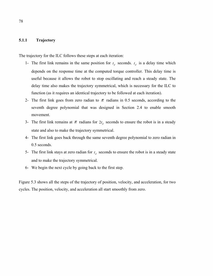
78
5.1.1 Trajectory
The trajectory for the ILC follows these steps at each iteration:
1- The first link remains in the same position for seconds. is a delay time which
depends on the response time at the computed torque controller. This delay time is
useful because it allows the robot to stop oscillating and reach a steady state. The
delay time also makes the trajectory symmetrical, which is necessary for the ILC to
function (as it requires an identical trajectory to be followed at each iteration).
2- The first link goes from zero radian to radians in 0.5 seconds, according to the
seventh degree polynomial that was designed in Section 2.4 to enable smooth
movement.
3- The first link remains at radians for seconds to ensure the robot is in a steady
state and also to make the trajectory symmetrical.
4- The first link goes back through the same seventh degree polynomial to zero radian in
0.5 seconds.
5- The first link stays at zero radian for seconds to ensure the robot is in a steady state
and to make the trajectory symmetrical.
6- We begin the next cycle by going back to the first step.
Figure 5.3 shows all the steps of the trajectory of position, velocity, and acceleration, for two
cycles. The position, velocity, and acceleration all start smoothly from zero.
dt dt
π
π 2 dt
dt

79
Figure 5.3 Two successive cycles of trajectory of position, velocity and acceleration
In order to test the computed torque controller in the simulation, only the first cycle of the
trajectory is used.
The required torque for this trajectory is shown in Figure 5.4.

80
Figure 5.4 Required torque for the trajectory described in this section
Figure 5.4 shows that the maximum absolute value of the required torque is less than 0.04
N.m. The nominal torque (maximum continuous torque) for the motor on this robot is 128
mN.m, which is greater than the maximum required torque for this trajectory. So there is no
problem for the robot motor to follow this trajectory. In other words, it is feasible, as required
by the ILC assumption stated in Section 1.3.3. In Figure 5.4 we see that close to 0.8 s and 2.1
s the torque is oscillating a little. In these two moments the robot is close to its singularity.
That is why we see some oscillation in the torque.
The mechanical parameters of the four-bars robot were presented in Table 2.1.
81
5.1.2 Computed torque results
In equation (2.89) we set the response time equal to 0.25 s for the PID computed torque
controller. The values of , and are determined from
Erreur ! Source du renvoi introuvable., Erreur ! Source du renvoi introuvable. and
(2.88) respectively:
23 1887.0192p λ= =K I
3 15775.48051i λ= =K I
3 75.24d λ= =K I
Figure 5.5 shows the position error of the closed loop system in radians for one cycle (or
one iteration). The desired trajectory is one cycle of Figure 5.3.
pK iK dK
6.2725.08
rTλ = =
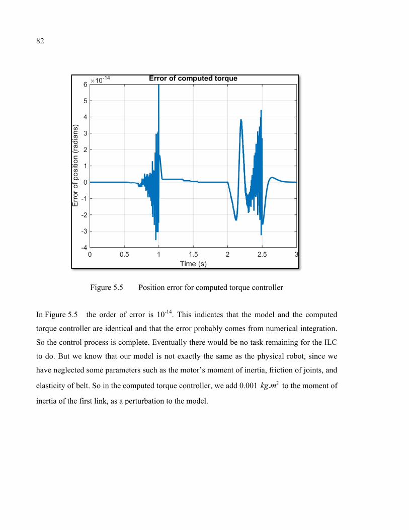
82
Figure 5.5 Position error for computed torque controller
In Figure 5.5 the order of error is 10-14. This indicates that the model and the computed
torque controller are identical and that the error probably comes from numerical integration.
So the control process is complete. Eventually there would be no task remaining for the ILC
to do. But we know that our model is not exactly the same as the physical robot, since we
have neglected some parameters such as the motor’s moment of inertia, friction of joints, and
elasticity of belt. So in the computed torque controller, we add 0.001 to the moment of
inertia of the first link, as a perturbation to the model.
2.kg m

83
Figure 5.6 Position error for perturbed computed torque controller
Figure 5.6 depicts the error of the perturbed computed torque controller. In this case we can
better verify the effect of ILC on the system. All the simulations from now on are done with
the perturbed model.
5.1.3 Results of computed torque with ILC
Here the two types of ILC are combined with the computed torque. This section describes
how they are tested, and presents the results. 200 iterations are performed for each test and
the is 0.5 seconds. In other words, the cycle time is 3 seconds. The response time of the
computed torque for all the tests is 0.25 seconds.
dt
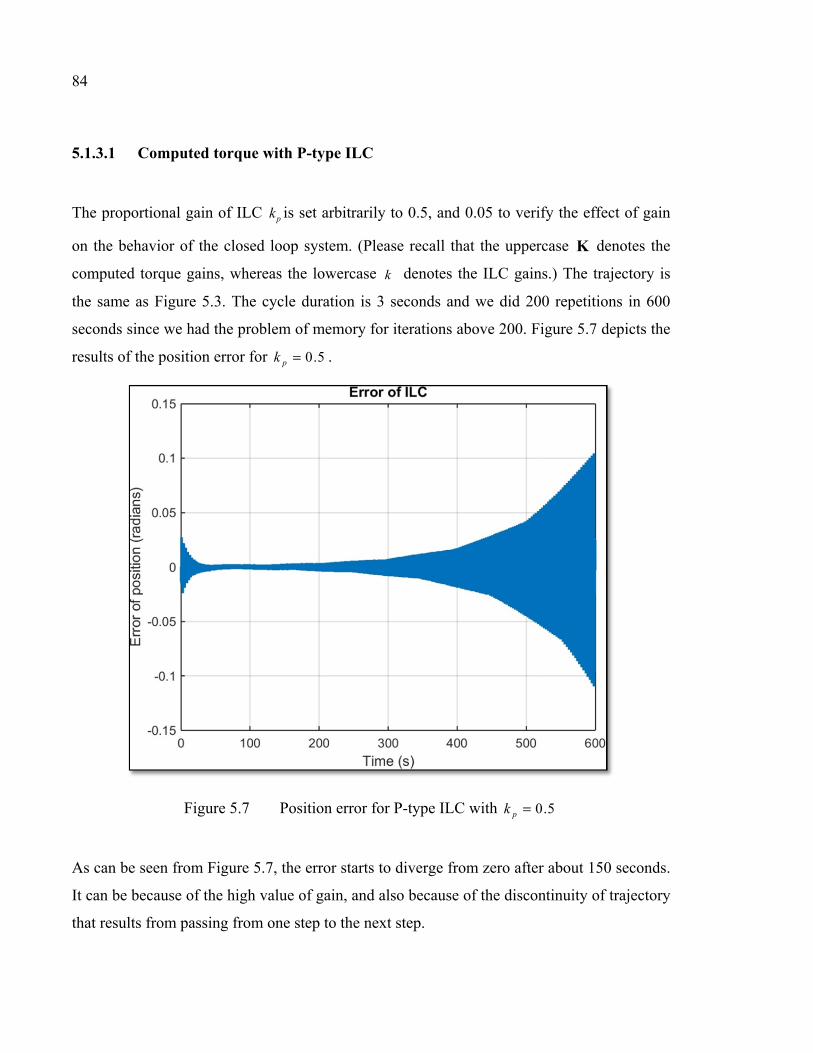
84
5.1.3.1 Computed torque with P-type ILC
The proportional gain of ILC is set arbitrarily to 0.5, and 0.05 to verify the effect of gain
on the behavior of the closed loop system. (Please recall that the uppercase denotes the
computed torque gains, whereas the lowercase denotes the ILC gains.) The trajectory is
the same as Figure 5.3. The cycle duration is 3 seconds and we did 200 repetitions in 600
seconds since we had the problem of memory for iterations above 200. Figure 5.7 depicts the
results of the position error for .
Figure 5.7 Position error for P-type ILC with
As can be seen from Figure 5.7, the error starts to diverge from zero after about 150 seconds.
It can be because of the high value of gain, and also because of the discontinuity of trajectory
that results from passing from one step to the next step.
pk
K
k
0.5pk =
0.5pk =

85
In the next step we decrease the gain to in order to see if the error converges to
zero.
Figure 5.8 Position error for P-type ILC with
From Figure 5.8 one may observe a good but slow convergence of error to zero. However,
we can still see that the error might diverge if we continued the procedure. It seems that
is satisfying for the case of P-type ILC during 600 seconds. The convergence can
be better seen in Figure 5.9, which shows the RMS of error. The RMS of error is calculated
using equation (5.1), as follows:
(5.1)
0.05pk =
0.05pk =
0.05pk =
2
1
1 n
RMS ii
error en =
=
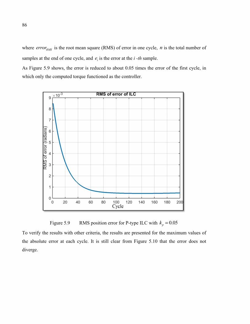
86
where is the root mean square (RMS) of error in one cycle, is the total number of
samples at the end of one cycle, and is the error at the i -th sample.
As Figure 5.9 shows, the error is reduced to about 0.05 times the error of the first cycle, in
which only the computed torque functioned as the controller.
Figure 5.9 RMS position error for P-type ILC with
To verify the results with other criteria, the results are presented for the maximum values of
the absolute error at each cycle. It is still clear from Figure 5.10 that the error does not
diverge.
RMSerror n
ie
0.05pk =
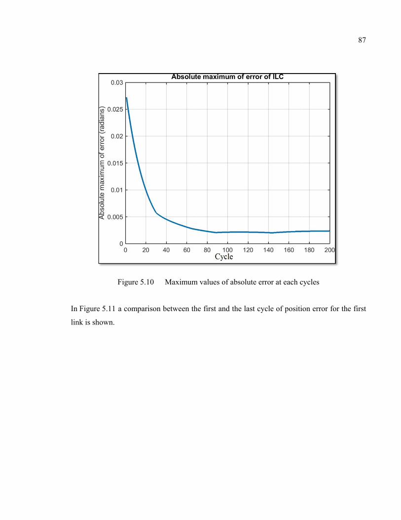
87
Figure 5.10 Maximum values of absolute error at each cycles
In Figure 5.11 a comparison between the first and the last cycle of position error for the first
link is shown.

88
Figure 5.11 Comparison between the error of the first and the last cycles for P-type ILC
5.1.3.2 PD-type ILC
Here the results of PD-type ILC are presented. Since the error plots do not give any more
information than the RMS plots, from now on we will only present the RMS error for each
case.
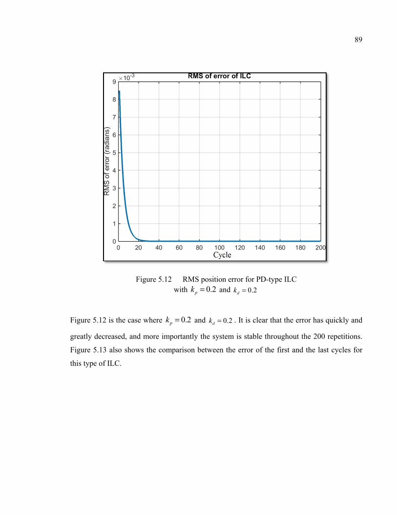
89
Figure 5.12 RMS position error for PD-type ILC with and
Figure 5.12 is the case where and . It is clear that the error has quickly and
greatly decreased, and more importantly the system is stable throughout the 200 repetitions.
Figure 5.13 also shows the comparison between the error of the first and the last cycles for
this type of ILC.
0.2pk = 0.2dk =
0.2pk = 0.2dk =
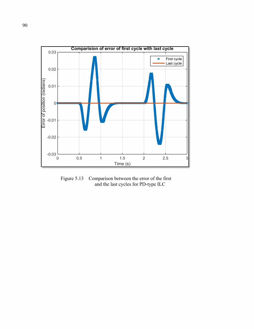
90
Figure 5.13 Comparison between the error of the first and the last cycles for PD-type ILC
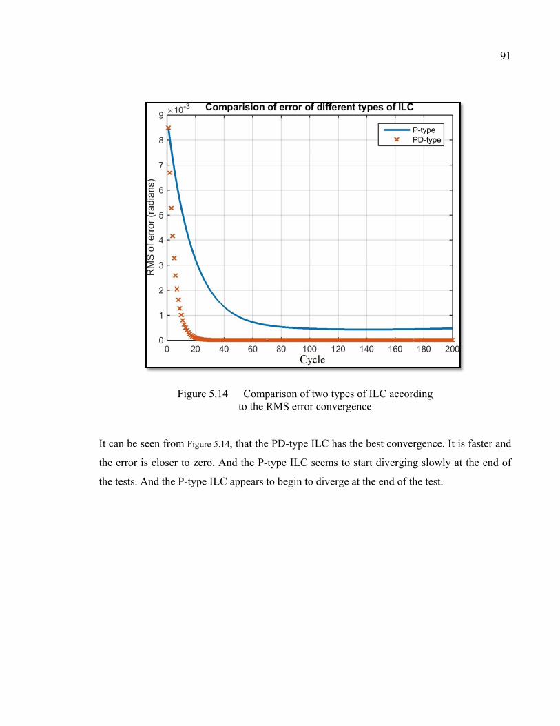
91
Figure 5.14 Comparison of two types of ILC according to the RMS error convergence
It can be seen from Figure 5.14, that the PD-type ILC has the best convergence. It is faster and
the error is closer to zero. And the P-type ILC seems to start diverging slowly at the end of
the tests. And the P-type ILC appears to begin to diverge at the end of the test.

CHAPTER 6
EXPERIMENTAL RESULTS
6.1 Real robot
In this chapter the same trajectory as in the simulation is implemented with the real robot.
We use TwinCAT 3 compiler to compile exactly the same diagram-blocks of the controller in
Simulink that we used in the simulation, so it would be able to upload on TwinCAT 3
software. Figure 6-5 presents the setup.
6.2 Validation
We will validate the macro-generated SimMechanics model that was presented in Chapter
Three by comparing its performance during a simulation with that of the real robot during a
practical experiment.
6.2.1 SimMechanics
To ensure the macro described in Chapter Three functions sufficiently, we will generate the
SimMechanics file of the parallel robot from the CAD file in CATIA. By adding the actuator
and sensor, we will have the dynamic model of the robot in SimMechanics. For the
validation, two computed torque controllers are designed using SimMechanics and the rigid
model from the previous chapter. These two controllers are used to control the position of the
first link of the real robot. If the robot follows the trajectory with just a small error, then the
controller is performing well and we can conclude that the SimMechanics model is a good
approximation of the real robot.
Once we have the forward dynamic model in SimMechanics we can use it for inverse
dynamics too. With the inverse dynamic model, we can calculate the torque that is needed for
the robot to follow a specific trajectory. To obtain the inverse dynamics model, some of the
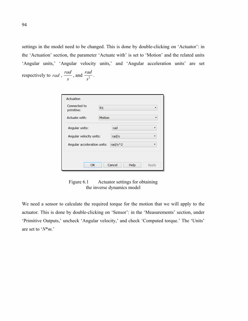
94
settings in the model need to be changed. This is done by double-clicking on ‘Actuator’: in
the ‘Actuation’ section, the parameter ‘Actuate with’ is set to ‘Motion’ and the related units
‘Angular units,’ ‘Angular velocity units,’ and ‘Angular acceleration units’ are set
respectively to , , and .
Figure 6.1 Actuator settings for obtaining the inverse dynamics model
We need a sensor to calculate the required torque for the motion that we will apply to the
actuator. This is done by double-clicking on ‘Sensor’: in the ‘Measurements’ section, under
‘Primitive Outputs,’ uncheck ‘Angular velocity,’ and check ‘Computed torque.’ The ‘Units’
are set to ‘N*m.’
radrad
s 2
rad
s

95
Figure 6.2 Sensor settings for obtaining the inverse dynamics model
It is possible to use this block for the computed torque. The position feedback from the real
robot is directly connected to the first input of the actuator, and the robot’s velocity feedback
is connected to the second input. In order to use the PID computed torque, the position error
is multiplied by the proportional gain Kp, the velocity error is multiplied by the derivative
gain Kd, and the integral of the position error is multiplied by the integral gain Ki calculated
in Section 2.5.1. The response time is 0.25 seconds. The sum of these three signals, plus the
desired acceleration, produces the signal that goes directly to the acceleration input of the
actuator. Figure 6.3 presents a schema of this implementation.

96
Figure 6.3 PID computed torque using inverse dynamic
After preparing the model, it must be compiled in a format that is compatible with the
software that communicates with the robot. On a computer where TwinCAT 3 is already
installed, we browse to find ‘TwinCAT.tlc’ in the following path from the SimMechanics file
that we have already prepared for the validation: ‘Configuration Parameters\ Code
Generation.’ In the ‘Target selection’ part, browse the ‘System target file’ to find
‘TwinCAT.tlc.’ Here we change the ‘Language’ to ‘C’ to enable compilation of the
SimMechanic blocks.
Figure 6.4 Configuring Simulink for TwinCAT file generation
After clicking on the ‘Build model’ button in the menu at the top of the window, Matlab will
begin to compile and generate the file for TwinCAT.
97
6.2.2 Hardware
For the controlling task, we use an industrial PC made by Beckhoff. The model of this PC is
C6920-0040. The operating system is real-time Windows 7. It makes it possible to run all the
executable software on Windows directly on the PC. This PC is also equipped with USB and
LAN ports.
The servo drive is from the Whistle series manufactured by Elmo Motion Control Ltd. This
digital servo drive is small but powerful (3200 W peak and 1600 W continuous power). It is
used for DC brush, brushless, and linear motors. The Elmo Whistle drive can operate in three
different modes: position, velocity and current. It is also equipped with a LAN port.
6.2.3 Connection
The connection between the servo drive and the industrial PC is through the LAN ports. The
protocol is EtherCAT. EtherCAT is developed by Beckhoff and is a real-time industrial
Ethernet. The EtherCAT protocol is suitable for hard and soft real-time requirements in
automation technology, testing, and measurement.
6.2.4 Software
TwinCAT (The Windows Control and Automation Technology) is the center of the control
system. TwinCAT 3 has many features. The most important one for our purposes is the
ability to link to Matlab/Simulink. It is possible to compile a Simulink file to generate a
TwinCAT file. Then we can load this file into TwinCAT 3 to run it in real time. In our case
the controller of the four-bar robot can also be compiled.
After compiling the SimMechanics model with the controller, we have the TwinCAT file that
will be loaded and configured in TwinCAT software. Before opening this file in TwinCAT
we need to make a new project in this software in which we define the inputs, outputs,
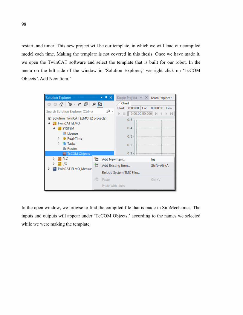
98
restart, and timer. This new project will be our template, in which we will load our compiled
model each time. Making the template is not covered in this thesis. Once we have made it,
we open the TwinCAT software and select the template that is built for our robot. In the
menu on the left side of the window in ‘Solution Explorer,’ we right click on ‘TcCOM
Objects \ Add New Item.’
In the open window, we browse to find the compiled file that is made in SimMechanics. The
inputs and outputs will appear under ‘TcCOM Objects,’ according to the names we selected
while we were making the template.

99
We double-click on each of the inputs and outputs and attach each signal to the appropriate
variable by double-clicking on it.
Then we double-click on the ‘Object’ under ‘TcCOM Objects,’ and in the second tab
‘Context’ we select the ‘Task’ that we defined while making the template. Here we have
named it ‘PID.’
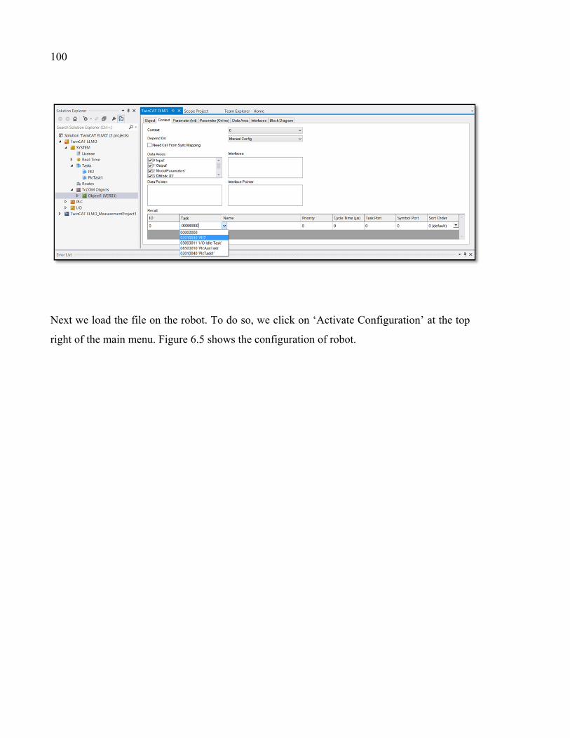
100
Next we load the file on the robot. To do so, we click on ‘Activate Configuration’ at the top
right of the main menu. Figure 6.5 shows the configuration of robot.

101
Figure 6.5 Robot setup
6.3 Experimental results
The experimental tests are done on the computed torque and the two types of ILC. This
section presents the plots of error and RMS error for these tests.
6.3.1 Computed torque results
We first verify the computed torque controller alone, before moving on to verification of the
ILC controllers. The desired trajectory is the same as the one we did our simulations with; it
is depicted in the first cycle of Figure 5.3. All the conditions are the same as in the simulation
part, including the value of the PID gains.
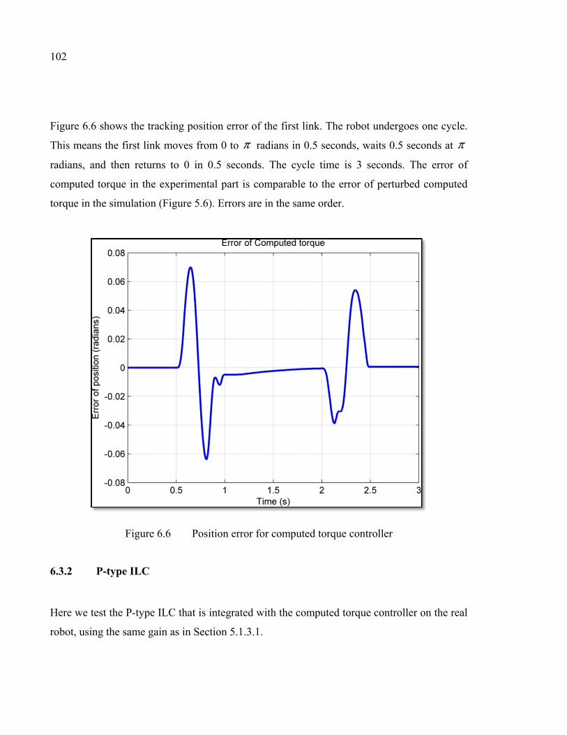
102
Figure 6.6 shows the tracking position error of the first link. The robot undergoes one cycle.
This means the first link moves from 0 to radians in 0.5 seconds, waits 0.5 seconds at
radians, and then returns to 0 in 0.5 seconds. The cycle time is 3 seconds. The error of
computed torque in the experimental part is comparable to the error of perturbed computed
torque in the simulation (Figure 5.6). Errors are in the same order.
Figure 6.6 Position error for computed torque controller
6.3.2 P-type ILC
Here we test the P-type ILC that is integrated with the computed torque controller on the real
robot, using the same gain as in Section 5.1.3.1.
π π
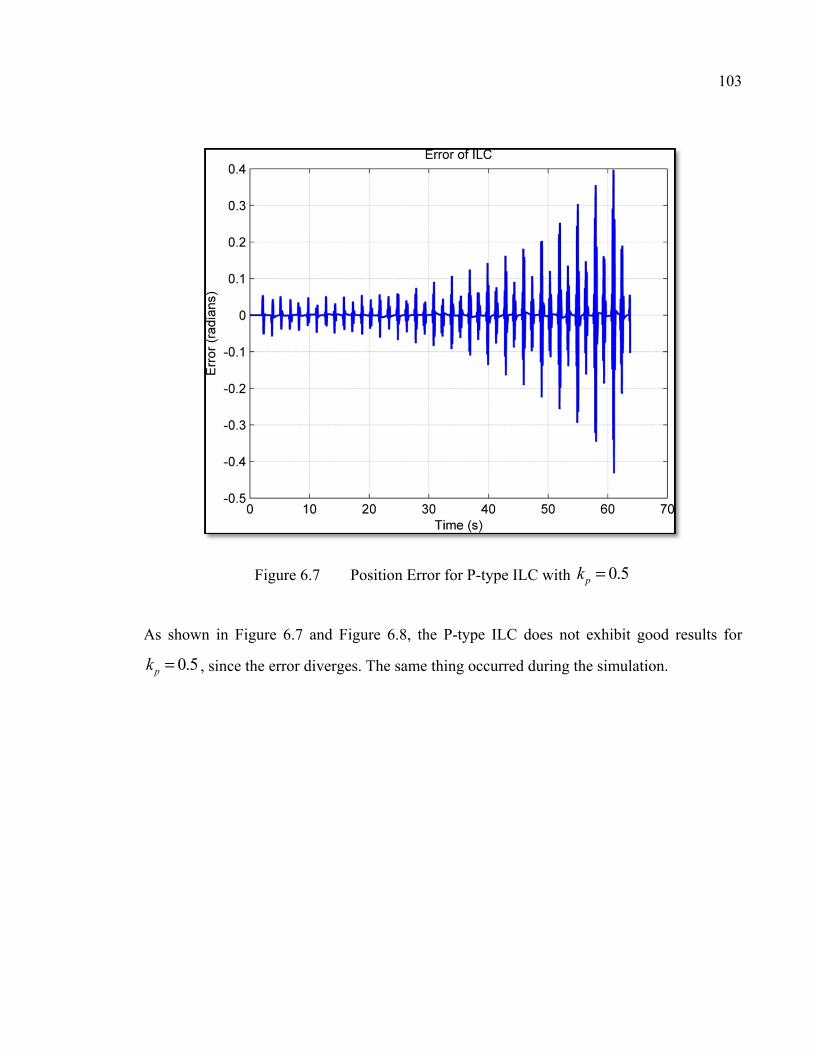
103
Figure 6.7 Position Error for P-type ILC with
As shown in Figure 6.7 and Figure 6.8, the P-type ILC does not exhibit good results for
, since the error diverges. The same thing occurred during the simulation.
0.5pk =
0.5pk =

104
Figure 6.8 RMS position error for P-type ILC with
To achieve an acceptable result by trial and error, we found that presents good
results for the P-type ILC when considering the RMS error. But Figure 6.9 shows there are
some peaks that seem to increase, so this would not be a good control approach for this
application.
0.5pk =
0.01pk =

105
Figure 6.9 Position error for P-type ILC with
0.01pk =
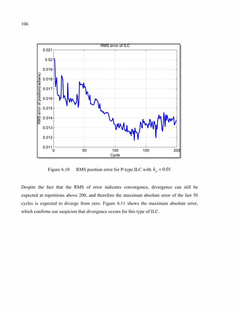
106
Figure 6.10 RMS position error for P-type ILC with
Despite the fact that the RMS of error indicates convergence, divergence can still be
expected at repetitions above 200, and therefore the maximum absolute error of the last 50
cycles is expected to diverge from zero. Figure 6.11 shows the maximum absolute error,
which confirms our suspicion that divergence occurs for this type of ILC.
0.01pk =
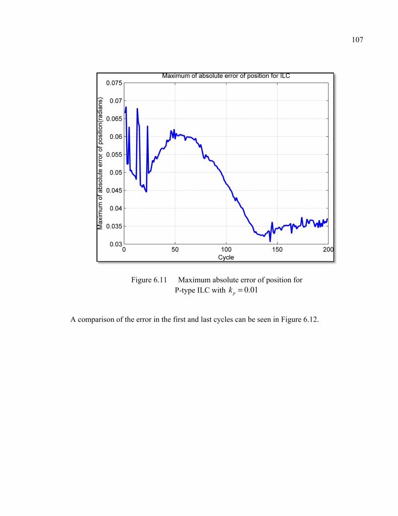
107
Figure 6.11 Maximum absolute error of position for P-type ILC with
A comparison of the error in the first and last cycles can be seen in Figure 6.12.
0.01pk =

108
Figure 6.12 Comparison of error in first and last cycles for P-type ILC with
Figure 6.12 shows that the error has overall been reduced, but still is not perfect.
6.3.3 PD-type ILC
Figure 6.13 shows better convergence of the RMS error for the PD-type ILC with
and , compared to the P-type ILC. The results indicate that the PD-type ILC is able
to shrink the error to approximately 0.25 times the error of the computed torque controller.
There is a bump at around the 60th cycle. ILC is very susceptible to change. During our
experiments, we found that even a small change in conditions (e.g. friction, stiffness, small
vibrations of the base of the robot, etc.) leads to a big change in the results.
0.01pk =
0.02pk =
0.02dk =
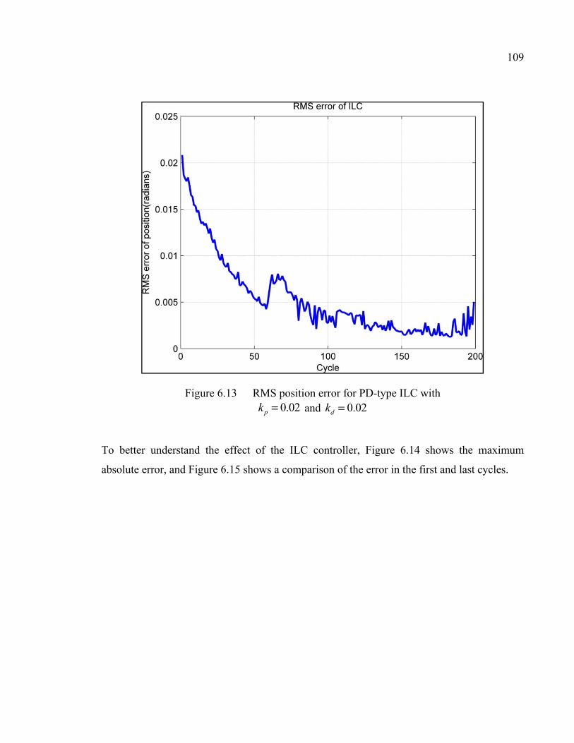
109
Figure 6.13 RMS position error for PD-type ILC with and
To better understand the effect of the ILC controller, Figure 6.14 shows the maximum
absolute error, and Figure 6.15 shows a comparison of the error in the first and last cycles.
0.02pk = 0.02dk =
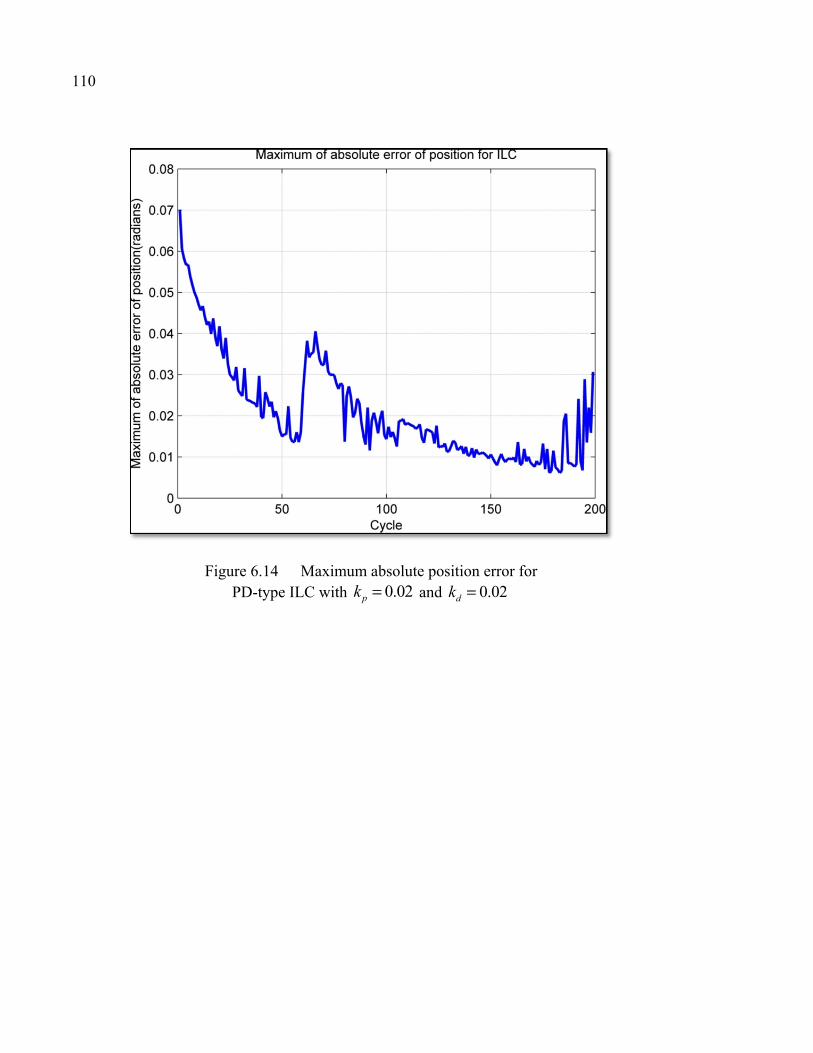
110
Figure 6.14 Maximum absolute position error for PD-type ILC with and 0.02pk = 0.02dk =
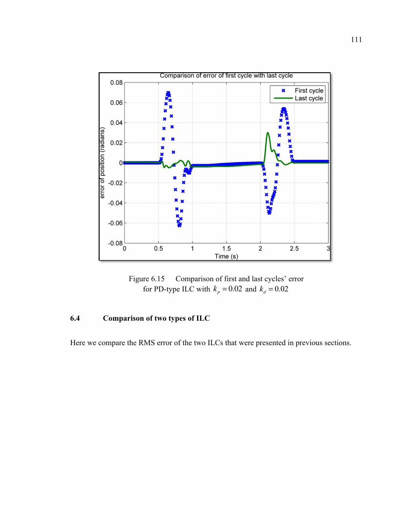
111
Figure 6.15 Comparison of first and last cycles’ error for PD-type ILC with and
6.4 Comparison of two types of ILC
Here we compare the RMS error of the two ILCs that were presented in previous sections.
0.02pk = 0.02dk =

112
Figure 6.16 Comparison of the RMS of error convergence for the two types of ILC
As seen from Figure 6.16, the PD-type ILC has the fastest convergence. The PD-type ILC
also exhibits the smallest values for error.
CONCLUSION….
In this thesis we modeled a four-bar parallel robot. This robot was selected because it is easy
to derive the equations of motion, and its dynamic model is non-linear. The dynamic model,
which we calculated manually, using the Lagrange method, treated the robot as composed of
four rigid components. After finding the equations of motion, we designed a computed
torque controller. We then made a simplified model of the robot in SimMechanics in order to
validate our manually-calculated (analytical) model. We compared the SimMechanics model
to the analytical model. The results show that the analytical model is reliable.
This thesis has validated a new method of virtual prototyping. The new method is to use a
macro that is added to CATIA V6 and enables the dynamic model to be generated and
exported to SimMechanics. Then any sensors and actuators can be added to the model in
SimMechanics, along with any other necessary modifications, to complete the dynamic
model. We used two control methods to validate the functionality of the macro: computed
torque and ILC. For the ILC we used two types, P-type and PD-type, which were used in
serial configuration with the computed torque and the robot. With these methods, we
conducted three simulations: the first used computed torque alone, the second used a
combination of computed torque and P-type ILC, and the third used a combination of
computed torque and PD-type ILC.
For the purpose of testing the controller combinations, a seventh degree polynomial was
designed for trajectory. This is a smooth and fast trajectory. The simulation results show that
the fastest convergence was done by the combination of computed torque and PD-type ILC.
This combination also resulted in the smallest error value.
To compare the performance of the model with the performance of the actual robot, the
actual robot was used with a Beckhoff controller for a controlling task. The results of the
practical experiment show that the PD-type ILC is preferable to the P-type (both types were
used in conjunction with the computed torque controller). We had to use smaller gains in the
114
practical experiment than in the simulation in order to prevent the error from diverging. The
error was bigger in the practical experiment than in the simulation. This could be because in
our virtual model we did not take into account several factors that affect the real robot, such
as friction, the mass of screws and bolts, the moment of inertia of the rotor and pulleys, and
the stiffness of the timing belt.
RECOMMENDATIONS
We have several recommendations for future research. Several changes should be made in
hardware as well as software. First, regarding software we recommend trying other
configurations of the controller. For example, the ILC controller parallel could be made with
computed torque instead of the serial structure that we verified in this paper. Second, we
recommend changing the trajectory to observe the effect of other trajectories. Here, the
trajectory of the first link was , but one might experiment with another trajectory such
as and do a complete circle. Third, there are many other types of ILCs apart from
those we mentioned. For instance, we suggest testing the ILC when using the CITE
approach, which uses previous and actual cycle error. Finally, during virtual prototyping we
only considered three types of joint constraints: revolute, prismatic and fixed. Future
researchers might improve upon our work by including other types of joint constraints such
as gear or universal.
[0, ]π
[0,2 ]π

LIST OF REFERENCES
Ahn, Hyo-Sung, Kevin L. Moore and YangQuan Chen. 2007. Iterative learning control :
robustness and monotonic convergence for interval systems. Coll. « Communications and control engineering ». London: Springer, xviii, 230 p. p.
Arimoto, S, S Kawamura and F Miyazaki. 1986. « Convergence, stability and robustness of
learning control schemes for robot manipulators ». In Proceedings of the International Symposium on Robot Manipulators on Recent trends in robotics: modeling, control and education. (Albuquerque, New Mexico, USA), p. 307-316. 23632: Elsevier North-Holland, Inc.
Arimoto, S. 1985. « Mathematical theory of learning with applications to robot control ».
Proceedings of 4th Yale Workshop on Applications of Adaptive Systems, p. 379-388. Arimoto, Suguru, Sadao Kawamura and Fumio Miyazaki. 1984. « Bettering operation of
Robots by learning ». Journal of Robotic Systems, vol. 1, no 2, p. 123-140. Bien, Z., and K.M. Huh. 1989. « Higher-order iterative learning control algorithm ». IEE
Proceedings D (Control Theory and Applications). Vol. 136, no 3, p. 105-112. < http://digital-library.theiet.org/content/journals/10.1049/ip-d.1989.0016 >.
Bondi, P., G. Casalino and L. Gambardella. 1988. « On the iterative learning control theory
for robotic manipulators ». Robotics and Automation, IEEE Journal of, vol. 4, no 1, p. 14-22.
Bonev, Ilian. 2013. « Mecademic ». < www.mecademic.com >. Craig, J. 1984. « Adaptive control of manipulators through repeated trials ». In Proceedings
of 1984 American Control Conference. (San Diego, California), p. 1566-1572. Craig, John J. 2005. Introduction to robotics: mechanics and control, 3. Pearson Prentice
Hall Upper Saddle River. Edwards, J. B. 1974. « Stability problems in the control of multipass processes ». Electrical
Engineers, Proceedings of the Institution of, vol. 121, no 11, p. 1425-1432. Gauthier, Guy. 2008. « Terminal iterative learning for cycle-to-cycle control of industrial
processes ». In /z-wcorg/. http://worldcat.org. Gu, You-Liang, and NanK Loh. 1989. « Learning control in robotic systems ». Journal of
Intelligent and Robotic Systems, vol. 2, no 2-3, p. 297-305.

118
Harokopos, E. 1986. « Optimal learning control of mechanical manipulators in repetitive motions ». In Robotics and Automation. Proceedings. 1986 IEEE International Conference on. (Apr 1986) Vol. 3, p. 396-401.
Hauser, J. 1987. « Learning control for a class of nonlinear systems ». In Proceedings of 26th
Conference on Decision and Control. (Los Angeles, California), p. 859-860. Heinzinger, Greg, D. Fenwick, B. Paden and F. Miyazaki. 1989. « Robust leaning control ».
In Decision and Control, 1989., Proceedings of the 28th IEEE Conference on. (13-15 Dec 1989), p. 436-440 vol.1.
Hideg, L. M., and R. P. Judd. 1988. « Frequency domain analysis of learning systems ». In
Decision and Control, 1988., Proceedings of the 27th IEEE Conference on. (7-9 Dec 1988), p. 586-591 vol.1.
Jagannathan, S. 2001. « Control of a multiple link robot arm at very high speeds for an
industrial application ». In American Control Conference, 2001. Proceedings of the 2001. Vol. 2, p. 793-798. IEEE.
Joubair, Ahmed. 2012. « Contribution à l’amélioration de la précision absolue des robots
parallèles ». École de technologie supérieure. Kato, T. Mita and E. 1985. « Iterative control and its application to motion control of robot
arm- adirect approach to servo-problems ». Proceedings of 24th Conference on Decision and Control, p. 1393.
M.Yamakita, K. Furuta and. 1987. « The design of a learning control system for
multivariable systems ». Proceedings of IEEE International Symoisium on Intelligent Control, p. 371-376.
McIntyre, C. Atkeson and J. 1986. « Robot trajectory learning through practice ».
Proceedings of IEEE Conference on Robotics and Automation. Merlet, J. P. 2006. Parallel robots, 2nd. Coll. « Solid mechanics and its applications », 74.
Dordrecht ; Boston, MA: Kluwer Academic Publishers, xiv, 355 p. p. Messner, W., R. Horowitz, W. W. Kao and Michael Boals. 1991. « A new adaptive learning
rule ». Automatic Control, IEEE Transactions on, vol. 36, no 2, p. 188-197. Moore, Kevin L. 1993. Iterative learning control for deterministic systems. Coll. « Advances
in industrial control ». London ; New York: Springer-Verlag, xvi, 152 p. p. Murray, Richard M, Zexiang Li, S Shankar Sastry and S Shankara Sastry. 1994. A
mathematical introduction to robotic manipulation. CRC press.
119
Sang-Rok, Oh, Bien Zeungnam and Suh Il Hong. 1988. « An iterative learning control method with application to robot manipulators ». Robotics and Automation, IEEE Journal of, vol. 4, no 5, p. 508-514.
Sugie, Toshiharu, and Toshiro Ono. 1991. « An iterative learning control law for dynamical
systems ». Automatica, vol. 27, no 4, p. 729-732. Tsai, Lung-Wen. 1999. Robot analysis : the mechanics of serial and parallel manipulators.
New York: Wiley, xiii, 505 p. p. Uchiyama, M. 1978. « Formation of high speed motion pattern of mechanical arm by trial ».
Transactions of the Society of Instrumentation and Control Engineers, vol. 19, p. 706-712.
Yamakita, M., and K. Furuta. 1991. « Iterative Generation of Virtual Reference for a
Manipulator ». Robotica, vol. 9, no 01, p. 71-80. Yamano, M. Togai and O. 1985. « Analysis and design of an optimal learning control
system: a discrete system approach ». In Proceedings of 24th Conference on Decision and Control. (Florida), p. 1399-1404.
Yang Quan, Chen, and K. L. Moore. 2002. « An optimal design of PD-type iterative learning
control with monotonic convergence ». In Intelligent Control, 2002. Proceedings of the 2002 IEEE International Symposium on. (2002), p. 55-60.
Yeon, Je Sung, Eui Jin Kim, Sang-Hun Lee, Jong Hyeon Park and Jong-Sung Hur. 2005. «
Development of Inverse Dynamic Controller for Industrial robots with HyRoHILS system ». In Proceedings of International Conference on Control, Automation and Systems (ICCAS 2005), Korea, Kyeonggi-Do.