Ecography ECOG-02034Heino, J. and de Mendoza, G. 2016. Predictability of stream insect distributions is dependent on niche position, but not on biological traits or taxonomic relatedness of species. – Ecography doi: 10.1111/ecog.02034

Supplementary material

1

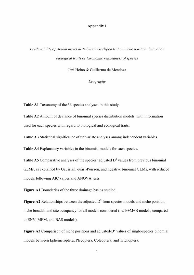
Appendix 1

Predictability of stream insect distributions is dependent on niche position, but not on

biological traits or taxonomic relatedness of species

Jani Heino & Guillermo de Mendoza

Ecography

Table A1 Taxonomy of the 36 species analysed in this study.

Table A2 Amount of deviance of binomial species distribution models, with information

used for each species with regard to biological and ecological traits.

Table A3 Statistical significance of univariate analyses among independent variables.

Table A4 Explanatory variables in the binomial models for each species.

Table A5 Comparative analyses of the species’ adjusted D2 values from previous binomial

GLMs, as explained by Gaussian, quasi-Poisson, and negative binomial GLMs, with reduced

models following AIC values and ANOVA tests.

Figure A1 Boundaries of the three drainage basins studied.

Figure A2 Relationships between the adjusted D2 from species models and niche position,

niche breadth, and site occupancy for all models considered (i.e. E+M+B models, compared

to ENV, MEM, and BAS models).

Figure A3 Comparison of niche positions and adjusted-D2 values of single-species binomial

models between Ephemeroptera, Plecoptera, Coleoptera, and Trichoptera.

2

Table A1. Taxonomy of the 36 stream insect species (class Insecta) analysed in this study, following de Jong et al. (2014).

Order Family Genus Species Ephemeroptera Baetidae Baetis B. muticus (Linnaeus 1758) Ephemeroptera Baetidae Baetis B. niger (Linnaeus 1761) Ephemeroptera Baetidae Baetis B. rhodani (Pictet 1843) Ephemeroptera Ameletidae Ameletus A. inopinatus Eaton 1887 Ephemeroptera Heptageniidae Heptagenia H. dalecarlica Bengtsson 1912 Ephemeroptera Leptophlebiidae Habrophlebia H. lauta Eaton 1884 Ephemeroptera Leptophlebiidae Leptophlebia L. marginata (Linnaeus 1767) Ephemeroptera Ephemerellidae Ephemerella E. aroni Eaton 1908 Plecoptera Perlodidae Diura D. bicaudata (Linnaeus 1758) Plecoptera Perlodidae Diura D. nanseni (Kempny 1900) Plecoptera Perlodidae Isoperla I. difformis (Klapalek 1909) Plecoptera Perlodidae Isoperla I. grammatica (Poda 1761) Plecoptera Chloroperlidae Siphonoperla S. burmeisteri (Pictet 1841) Plecoptera Nemouridae Amphinemura A. borealis (Morton 1894) Plecoptera Nemouridae Amphinemura A. sulcicollis (Stephens 1836) Plecoptera Nemouridae Protonemura P. intricata (Ris 1902) Plecoptera Nemouridae Protonemura P. meyeri (Pictet 1841) Plecoptera Capniidae Capnopsis C. schilleri (Rostock 1892) Plecoptera Leuctridae Leuctra L. digitata Kempny 1899 Plecoptera Leuctridae Leuctra L. hippopus Kempny 1899 Plecoptera Leuctridae Leuctra L. nigra (Olivier 1811) Coleoptera Hydraenidae Hydraena H. gracilis Germar 1824 Coleoptera Elmidae Elmis E. aenea (Muller 1806) Coleoptera Elmidae Limnius L. volckmari (Panzer 1793) Coleoptera Elmidae Oulimnius O. tuberculatus (Muller 1806) Megaloptera Sialidae Sialis S. fuliginosa Pictet 1836 Trichoptera Rhyacophilidae Rhyacophila R. nubila Zetterstedt 1840 Trichoptera Rhyacophilidae Rhyacophila R. obliterata McLachlan 1863 Trichoptera Polycentropodidae Plectrocnemia P. conspersa (Curtis 1834) Trichoptera Polycentropodidae Polycentropus P. flavomaculatus (Pictet 1834) Trichoptera Hydropsychidae Hydropsyche H. angustipennis (Curtis 1834) Trichoptera Hydropsychidae Hydropsyche H. saxonica McLachlan 1884 Trichoptera Brachycentridae Micrasema M. gelidum McLachlan 1876 Trichoptera Limnephilidae Potamophylax P. cingulatus (Stephens 1837) Trichoptera Goeridae Silo S. pallipes (Fabricius 1871) Trichoptera Sericostomatidae Sericostoma S. personatum (Kirby & Spence 1826)

Reference cited: de Jong, Y. et al. 2014. Fauna Europaea: all animal species on the web. – Biodiversity Data Journal 2: e4034.

3

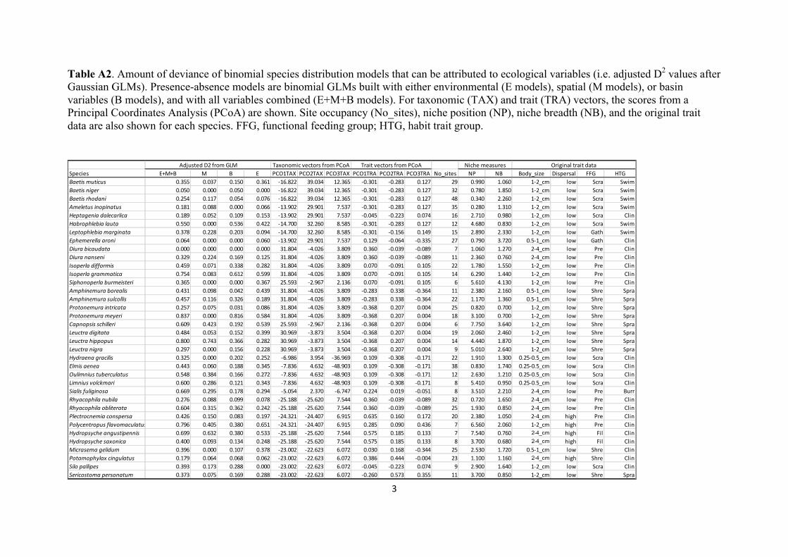
Table A2. Amount of deviance of binomial species distribution models that can be attributed to ecological variables (i.e. adjusted D2 values after Gaussian GLMs). Presence-absence models are binomial GLMs built with either environmental (E models), spatial (M models), or basin variables (B models), and with all variables combined (E+M+B models). For taxonomic (TAX) and trait (TRA) vectors, the scores from a Principal Coordinates Analysis (PCoA) are shown. Site occupancy (No_sites), niche position (NP), niche breadth (NB), and the original trait data are also shown for each species. FFG, functional feeding group; HTG, habit trait group.

Species E+M+B M B E PCO1TAX PCO2TAX PCO3TAX PCO1TRA PCO2TRA PCO3TRA No_sites NP NB Body_size Dispersal FFG HTGBaetismuticus 0.355 0.037 0.150 0.361 -16.822 39.034 12.365 -0.301 -0.283 0.127 29 0.990 1.060 1-2_cm low Scra SwimBaetisniger 0.050 0.000 0.050 0.000 -16.822 39.034 12.365 -0.301 -0.283 0.127 32 0.780 1.850 1-2_cm low Scra SwimBaetisrhodani 0.254 0.117 0.054 0.076 -16.822 39.034 12.365 -0.301 -0.283 0.127 48 0.340 2.260 1-2_cm low Scra SwimAmeletusinopinatus 0.181 0.088 0.000 0.066 -13.902 29.901 7.537 -0.301 -0.283 0.127 35 0.280 1.310 1-2_cm low Scra SwimHeptageniadalecarlica 0.189 0.052 0.109 0.153 -13.902 29.901 7.537 -0.045 -0.223 0.074 16 2.710 0.980 1-2_cm low Scra ClinHabrophlebialauta 0.550 0.000 0.536 0.422 -14.700 32.260 8.585 -0.301 -0.283 0.127 12 4.680 0.830 1-2_cm low Scra SwimLeptophlebiamarginata 0.378 0.228 0.203 0.094 -14.700 32.260 8.585 -0.301 -0.156 0.149 15 2.890 2.330 1-2_cm low Gath SwimEphemerellaaroni 0.064 0.000 0.000 0.060 -13.902 29.901 7.537 0.129 -0.064 -0.335 27 0.790 3.720 0.5-1_cm low Gath ClinDiurabicaudata 0.000 0.000 0.000 0.000 31.804 -4.026 3.809 0.360 -0.039 -0.089 7 1.060 1.270 2-4_cm low Pre ClinDiurananseni 0.329 0.224 0.169 0.125 31.804 -4.026 3.809 0.360 -0.039 -0.089 11 2.360 0.760 2-4_cm low Pre ClinIsoperladifformis 0.459 0.071 0.338 0.282 31.804 -4.026 3.809 0.070 -0.091 0.105 22 1.780 1.550 1-2_cm low Pre ClinIsoperlagrammatica 0.754 0.083 0.612 0.599 31.804 -4.026 3.809 0.070 -0.091 0.105 14 6.290 1.440 1-2_cm low Pre ClinSiphonoperlaburmeisteri 0.365 0.000 0.000 0.367 25.593 -2.967 2.136 0.070 -0.091 0.105 6 5.610 4.130 1-2_cm low Pre ClinAmphinemuraborealis 0.431 0.098 0.042 0.439 31.804 -4.026 3.809 -0.283 0.338 -0.364 11 2.380 2.160 0.5-1_cm low Shre SpraAmphinemurasulcollis 0.457 0.116 0.326 0.189 31.804 -4.026 3.809 -0.283 0.338 -0.364 22 1.170 1.360 0.5-1_cm low Shre SpraProtonemuraintricata 0.257 0.075 0.031 0.086 31.804 -4.026 3.809 -0.368 0.207 0.004 25 0.820 0.700 1-2_cm low Shre SpraProtonemurameyeri 0.837 0.000 0.816 0.584 31.804 -4.026 3.809 -0.368 0.207 0.004 18 3.100 0.700 1-2_cm low Shre SpraCapnopsisschilleri 0.609 0.423 0.192 0.539 25.593 -2.967 2.136 -0.368 0.207 0.004 6 7.750 3.640 1-2_cm low Shre SpraLeuctradigitata 0.484 0.053 0.152 0.399 30.969 -3.873 3.504 -0.368 0.207 0.004 19 2.060 2.460 1-2_cm low Shre SpraLeuctrahippopus 0.800 0.743 0.366 0.282 30.969 -3.873 3.504 -0.368 0.207 0.004 14 4.440 1.870 1-2_cm low Shre SpraLeuctranigra 0.297 0.000 0.156 0.228 30.969 -3.873 3.504 -0.368 0.207 0.004 9 5.010 2.640 1-2_cm low Shre SpraHydraenagracilis 0.325 0.000 0.202 0.252 -6.986 3.954 -36.969 0.109 -0.308 -0.171 22 1.910 1.300 0.25-0.5_cm low Scra ClinElmisaenea 0.443 0.060 0.188 0.345 -7.836 4.632 -48.903 0.109 -0.308 -0.171 38 0.830 1.740 0.25-0.5_cm low Scra ClinOulimniustuberculatus 0.548 0.384 0.166 0.272 -7.836 4.632 -48.903 0.109 -0.308 -0.171 12 2.630 1.210 0.25-0.5_cm low Scra ClinLimniusvolckmari 0.600 0.286 0.121 0.343 -7.836 4.632 -48.903 0.109 -0.308 -0.171 8 5.410 0.950 0.25-0.5_cm low Scra ClinSialisfuliginosa 0.669 0.295 0.178 0.294 -5.054 2.370 -6.747 0.224 0.019 -0.051 8 3.510 2.210 2-4_cm low Pre BurrRhyacophilanubila 0.276 0.088 0.099 0.078 -25.188 -25.620 7.544 0.360 -0.039 -0.089 32 0.720 1.650 2-4_cm low Pre ClinRhyacophilaobliterata 0.604 0.315 0.362 0.242 -25.188 -25.620 7.544 0.360 -0.039 -0.089 25 1.930 0.850 2-4_cm low Pre ClinPlectrocnemiaconspersa 0.426 0.150 0.083 0.197 -24.321 -24.407 6.915 0.635 0.160 0.172 20 2.380 1.050 2-4_cm high Pre ClinPolycentropusflavomaculatus 0.796 0.405 0.380 0.651 -24.321 -24.407 6.915 0.285 0.090 0.436 7 6.560 2.060 1-2_cm high Pre ClinHydropsycheangustipennis 0.699 0.632 0.380 0.533 -25.188 -25.620 7.544 0.575 0.185 0.133 7 7.540 0.760 2-4_cm high Fil ClinHydropsychesaxonica 0.400 0.093 0.134 0.248 -25.188 -25.620 7.544 0.575 0.185 0.133 8 3.700 0.680 2-4_cm high Fil ClinMicrasemagelidum 0.396 0.000 0.107 0.378 -23.002 -22.623 6.072 0.030 0.168 -0.344 25 2.530 1.720 0.5-1_cm low Shre ClinPotamophylaxcingulatus 0.179 0.064 0.068 0.062 -23.002 -22.623 6.072 0.386 0.444 -0.004 23 1.100 1.160 2-4_cm high Shre ClinSilopallipes 0.393 0.173 0.288 0.000 -23.002 -22.623 6.072 -0.045 -0.223 0.074 9 2.900 1.640 1-2_cm low Scra ClinSericostomapersonatum 0.373 0.075 0.169 0.288 -23.002 -22.623 6.072 -0.260 0.573 0.355 11 3.700 0.850 1-2_cm low Shre Spra

OriginaltraitdataNichemeasuresTraitvectorsfromPCoATaxonomicvectorsfromPCoAAdjustedD2fromGLM

4

Table A3. Statistical significance (P-values) of univariate analyses among independent variables (i.e. site occupancy, niche characteristics, species trait and taxonomic variables). Because this includes continuous and categorical variables, and among the latter the number of categories also varies, statistical tests may refer to the significance of the Spearman correlation coefficient, to Kruskal-Wallis tests, to Mann-Whitney tests, or to Fisher’s exact tests on a contingency table. Overall, this implies that P-values are not always strictly comparable, yet still indicate to what extent two variables can be considered as correlated. Significant P-values (i.e. P < 0.05) are highlighted in boldface. Sites, site occupancy; NP, niche position; NB, niche breadth; DP, dispersal potential; BS, body size; FFG, functional feeding group; HTG, habit trait group; TRA, trait vector; TAX, taxonomic vector. Vectors are multivariate axes of a Principal Coordinates Analysis (PCoA) combining either trait or taxonomic variables.

Sites NP NB DP BS FFG HTG TRA-1 TRA-2 TRA-3 TAX-1 TAX-2 TAX-3 Sites - NP <0.001 - NB 0.983 0.974 - DP 0.184 0.170 0.104 - BS 0.664 0.625 0.088 0.033 - FFG 0.139 0.269 0.066 0.020 <0.001 - HTG 0.092 0.237 0.557 0.267 0.010 <0.001 - TRA-1 0.372 0.965 0.086 <0.001 <0.001 <0.001 <0.001 - TRA-2 0.128 0.179 0.916 0.081 0.004 <0.001 <0.001 0.588 - TRA-3 0.385 0.114 0.458 0.013 <0.001 0.308 0.067 0.622 0.873 - TAX-1 0.403 0.968 0.358 0.002 0.238 0.081 0.031 0.009 0.457 0.014 - TAX-2 0.122 0.184 0.048 0.002 0.006 <0.001 0.002 0.002 <0.001 0.955 0.123 - TAX-3 0.033 0.098 0.256 0.122 0.013 0.149 0.001 0.704 0.647 <0.001 <0.001 0.944 -

5

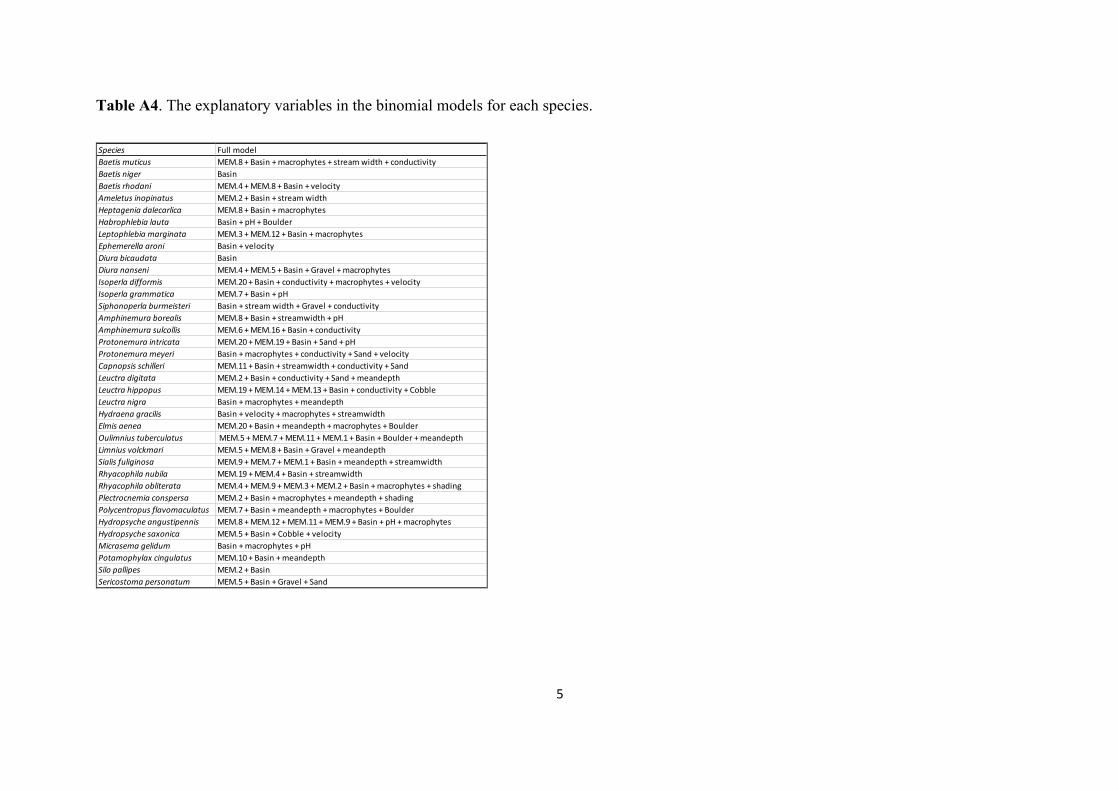
Table A4. The explanatory variables in the binomial models for each species.

Species FullmodelBaetismuticus MEM.8+Basin+macrophytes+streamwidth+conductivityBaetisniger BasinBaetisrhodani MEM.4+MEM.8+Basin+velocityAmeletusinopinatus MEM.2+Basin+streamwidthHeptageniadalecarlica MEM.8+Basin+macrophytesHabrophlebialauta Basin+pH+BoulderLeptophlebiamarginata MEM.3+MEM.12+Basin+macrophytesEphemerellaaroni Basin+velocityDiurabicaudata BasinDiurananseni MEM.4+MEM.5+Basin+Gravel+macrophytesIsoperladifformis MEM.20+Basin+conductivity+macrophytes+velocityIsoperlagrammatica MEM.7+Basin+pHSiphonoperlaburmeisteri Basin+streamwidth+Gravel+conductivityAmphinemuraborealis MEM.8+Basin+streamwidth+pHAmphinemurasulcollis MEM.6+MEM.16+Basin+conductivityProtonemuraintricata MEM.20+MEM.19+Basin+Sand+pHProtonemurameyeri Basin+macrophytes+conductivity+Sand+velocityCapnopsisschilleri MEM.11+Basin+streamwidth+conductivity+SandLeuctradigitata MEM.2+Basin+conductivity+Sand+meandepthLeuctrahippopus MEM.19+MEM.14+MEM.13+Basin+conductivity+CobbleLeuctranigra Basin+macrophytes+meandepthHydraenagracilis Basin+velocity+macrophytes+streamwidthElmisaenea MEM.20+Basin+meandepth+macrophytes+BoulderOulimniustuberculatus MEM.5+MEM.7+MEM.11+MEM.1+Basin+Boulder+meandepthLimniusvolckmari MEM.5+MEM.8+Basin+Gravel+meandepthSialisfuliginosa MEM.9+MEM.7+MEM.1+Basin+meandepth+streamwidthRhyacophilanubila MEM.19+MEM.4+Basin+streamwidthRhyacophilaobliterata MEM.4+MEM.9+MEM.3+MEM.2+Basin+macrophytes+shadingPlectrocnemiaconspersa MEM.2+Basin+macrophytes+meandepth+shadingPolycentropusflavomaculatus MEM.7+Basin+meandepth+macrophytes+BoulderHydropsycheangustipennis MEM.8+MEM.12+MEM.11+MEM.9+Basin+pH+macrophytesHydropsychesaxonica MEM.5+Basin+Cobble+velocityMicrasemagelidum Basin+macrophytes+pHPotamophylaxcingulatus MEM.10+Basin+meandepthSilopallipes MEM.2+BasinSericostomapersonatum MEM.5+Basin+Gravel+Sand

6

Table A5 Comparative analyses of the species’ adjusted D2 values from previous binomial GLMs (i.e. E, environmental models; M, spatial models; B, basin models; E+M+B, combined models), as explained by Gaussian (link = “identity”), quasi-Poisson (link = “log”), and negative binomial (link = “logit”), generalised linear models (GLMs), with niche characteristics, site occupancy, and trait and taxonomic vectors. PCO = principal coordinate, TRA = trait, TAX = taxonomy. PCOs thus describe the first three trait or taxonomic vectors. In the reduced model, variables are chosen following forward selection according to AIC values and ANOVA tests (i.e. Chi-square tests on a contingency table comparing two models at a time, specifically testing the significance of adding one variable to a previous, simpler model). AIC values could not be used in quasi-Poisson GLMs. The order in which the variables are added to the reduced models, is indicated by numbers in brackets. In negative binomial GLMs explaining the D2 of B models, the selection of the second and third variables is supported by ANOVA only. Significant P-values for variables in the full model (i.e. P < 0.05) are highlighted in boldface.

E models: Response Gaussian GLM Quasi-Poisson GLM Negative binomial GLM

D2 of E models Estimate SE t P Reduced Estimate SE t P Reduced Estimate SE t P Reduced

Intercept -0.099 0.107 -0.920 0.366 -2.509 0.514 -4.879 <0.001 -3.125 0.751 -4.160 <0.001

Site occupancy 0.008 0.003 2.348 0.027 0.025 0.017 1.461 0.156 0.046 0.024 1.917 0.066

Niche Position 0.092 0.018 5.099 <0.001 AIC/ANOVA (1) 0.283 0.073 3.896 <0.001 ANOVA (1) 0.518 0.132 3.934 <0.001 AIC/ANOVA (1)

Niche Breadth -0.033 0.028 -1.173 0.251 -0.134 0.121 -1.109 0.277 -0.202 0.183 -1.103 0.280

TRA-PCO1 -0.023 0.104 -0.223 0.826 -0.274 0.523 -0.525 0.604 -0.239 0.709 -0.337 0.738

TRA-PCO2 0.113 0.152 0.742 0.465 0.382 0.780 0.490 0.628 0.854 1.026 0.833 0.413

TRA-PCO3 -0.060 0.156 -0.384 0.704 -0.037 0.709 -0.052 0.959 -0.460 0.966 -0.476 0.638

TAX-PCO1 0.001 0.001 1.070 0.294 0.004 0.005 0.765 0.451 0.006 0.008 0.817 0.421

TAX-PCO2 0.000 0.002 -0.027 0.979 -0.003 0.011 -0.321 0.751 0.000 0.013 0.027 0.979

TAX-PCO3 -0.002 0.002 -0.906 0.373 -0.008 0.008 -1.053 0.302 -0.012 0.010 -1.160 0.256

7

M models: Response Gaussian GLM Quasi-Poisson GLM Negative binomial GLM

D2 of M models Estimate SE t P Reduced Estimate SE t P Reduced Estimate SE t P Reduced

Intercept -0.024 0.147 -0.166 0.870 -2.705 0.981 -2.756 0.011 -2.757 1.178 -2.340 0.0272

Site occupancy 0.003 0.005 0.535 0.597 0.002 0.034 0.054 0.956 0.006 0.040 0.149 0.883

Niche Position 0.055 0.025 2.232 0.035 AIC/ANOVA (1) 0.260 0.132 1.976 0.059 ANOVA (1) 0.335 0.181 1.848 0.076 AIC/ANOVA (1)

Niche Breadth -0.020 0.038 -0.518 0.609 -0.104 0.237 -0.439 0.664 -0.148 0.296 -0.499 0.622

TRA-PCO1 0.036 0.142 0.255 0.801 -0.111 0.920 -0.121 0.905 -0.088 1.109 -0.079 0.937

TRA-PCO2 0.060 0.208 0.287 0.777 0.139 1.347 0.103 0.919 0.149 1.601 0.093 0.927

TRA-PCO3 -0.048 0.213 -0.224 0.825 -0.233 1.322 -0.176 0.862 -0.271 1.640 -0.165 0.870

TAX-PCO1 -0.001 0.002 -0.333 0.742 -0.003 0.010 -0.283 0.780 -0.003 0.012 -0.275 0.786

TAX-PCO2 0.000 0.003 -0.076 0.940 -0.009 0.019 -0.488 0.630 -0.010 0.022 -0.437 0.666

TAX-PCO3 -0.001 0.002 -0.449 0.657 -0.009 0.014 -0.609 0.548 -0.010 0.017 -0.596 0.556

B models:

Response Gaussian GLM Quasi-Poisson GLM Negative binomial GLM

D2 of B models Estimate SE t P Reduced Estimate SE t P Reduced Estimate SE t P Reduced

Intercept 0.069 0.126 0.551 0.586 -2.052 0.563 -3.646 0.001 -2.075 0.759 -2.732 0.011

Site occupancy 0.006 0.004 1.491 0.148 0.023 0.019 1.208 0.238 0.035 0.026 1.353 0.188

Niche Position 0.070 0.021 3.276 0.003 AIC/ANOVA (1) 0.292 0.080 3.656 0.001 ANOVA (1) 0.408 0.124 3.296 0.003 AIC/ANOVA (1)

Niche Breadth -0.111 0.033 -3.379 0.002 AIC/ANOVA (2) -0.648 0.156 -4.169 <0.001 ANOVA (2) -0.838 0.221 -3.784 <0.001 ANOVA (2)

TRA-PCO1 -0.151 0.122 -1.246 0.224 -1.466 0.538 -2.725 0.011 ANOVA (3) -1.681 0.747 -2.251 0.033 ANOVA (3)

TRA-PCO2 -0.233 0.178 -1.308 0.202 -1.705 0.744 -2.292 0.030 -2.105 1.071 -1.966 0.060

TRA-PCO3 -0.102 0.182 -0.558 0.581 0.002 0.828 0.003 0.998 -0.010 1.074 -0.010 0.992

TAX-PCO1 0.002 0.001 1.357 0.187 0.008 0.005 1.531 0.138 0.011 0.008 1.446 0.160

TAX-PCO2 -0.003 0.002 -1.136 0.266 -0.026 0.010 -2.519 0.018 -0.031 0.014 -2.190 0.038

TAX-PCO3 0.002 0.002 1.191 0.244 0.009 0.009 1.030 0.312 0.009 0.011 0.838 0.410

8

E+M+B models: Response Gaussian GLM Quasi-Poisson GLM Negative binomial GLM

D2 of E+M+B models Estimate SE t P Reduced Estimate SE t P Reduced Estimate SE t P Reduced

Intercept 0.123 0.130 0.950 0.351 -1.460 0.355 -4.109 <0.001 -1.914 0.672 -2.848 0.008

Site occupancy 0.007 0.004 1.763 0.090 0.014 0.012 1.190 0.245 0.038 0.021 1.782 0.086

Niche Position 0.094 0.022 4.296 <0.001 AIC/ANOVA (1) 0.190 0.052 3.617 0.001 ANOVA (1) 0.492 0.137 3.591 0.001 AIC/ANOVA (1)

Niche Breadth -0.066 0.034 -1.958 0.061 -0.174 0.091 -1.915 0.067 -0.316 0.175 -1.808 0.082

TRA-PCO1 -0.141 0.125 -1.126 0.271 -0.530 0.347 -1.528 0.138 -0.732 0.597 -1.225 0.231

TRA-PCO2 -0.075 0.183 -0.408 0.687 -0.338 0.499 -0.678 0.504 -0.275 0.835 -0.329 0.745

TRA-PCO3 -0.066 0.188 -0.354 0.726 -0.019 0.501 -0.038 0.970 -0.451 0.905 -0.499 0.622

TAX-PCO1 0.001 0.001 0.781 0.442 0.003 0.004 0.734 0.469 0.004 0.007 0.561 0.579

TAX-PCO2 -0.003 0.002 -1.426 0.166 -0.012 0.007 -1.826 0.079 -0.016 0.011 -1.467 0.154

TAX-PCO3 -0.001 0.002 -0.720 0.478 -0.004 0.005 -0.844 0.406 -0.009 0.010 -0.904 0.374

9

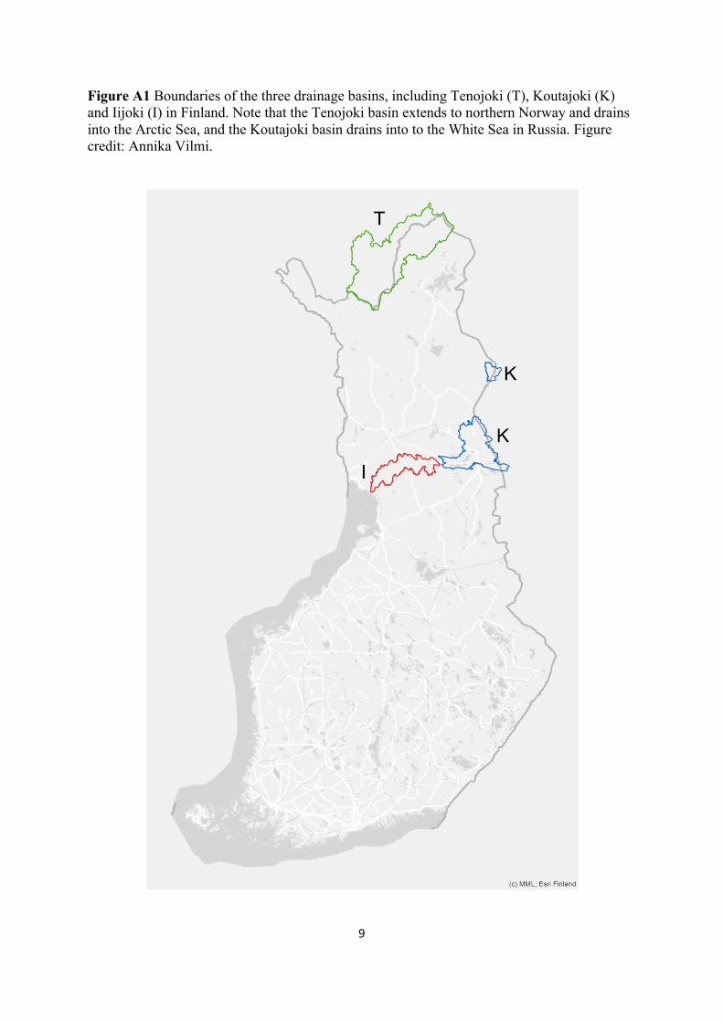
Figure A1 Boundaries of the three drainage basins, including Tenojoki (T), Koutajoki (K) and Iijoki (I) in Finland. Note that the Tenojoki basin extends to northern Norway and drains into the Arctic Sea, and the Koutajoki basin drains into to the White Sea in Russia. Figure credit: Annika Vilmi.

10

Figure A2 Scatterplots and significance of Spearman correlation coefficients showing the relationships between the adjusted D2 from species models and niche position (NP, from the OMI analysis), niche breadth (NB, from the OMI analysis) and site occupancy (sites), for all models considered (i.e. E+M+B models as shown in Fig. 6 of the main manuscript, compared to ENV, MEM, and BAS models). Asterisks indicate statistical significance: * P < 0.05, ** P < 0.01, *** P < 0.001.

11

Figure A3. Comparisons of niche positions (top) and adjusted-D2 values of single-species binomial models (bottom) between Ephemeroptera (Eph), Plecoptera (Plec), Coleoptera (Col), and Trichoptera (Trich). P-values refer to Kruskal-Wallis tests comparing all groups simultaneously.

Eph Plec Col Trich

0.0

0.2

0.4

0.6

0.8

1.0

Eph Plec Col Trich Eph Plec Col Trich Eph(a)

Plec(b)

Col(ab)

Trich(b)

Nic

he p

ositi

on

0

2

4

6

8

10

Eph(a)

Plec(b)

Col(ab)

Trich(ab)

E models (P ~ 0.223) M models (P ~ 0.307) B models (P ~ 0.545) E+M+B models (P ~ 0.083)

(P ~ 0.203)

0.0

0.2

0.4

0.6

0.8

1.0

0.0

0.2

0.4

0.6

0.8

1.0

Adj

uste

d-D

2 val

ue

0.0

0.2

0.4

0.6

0.8

1.0

Eph Plec Col Trich

0.0

0.2

0.4

0.6

0.8

1.0

Eph Plec Col Trich Eph Plec Col Trich Eph(a)

Plec(b)

Col(ab)

Trich(b)

Nic

he p

ositi

on

0

2

4

6

8

10

Eph(a)

Plec(b)

Col(ab)

Trich(ab)

E models (P ~ 0.223) M models (P ~ 0.307) B models (P ~ 0.545) E+M+B models (P ~ 0.083)

(P ~ 0.203)

0.0

0.2

0.4

0.6

0.8

1.0

0.0

0.2

0.4

0.6

0.8

1.0

Adj

uste

d-D

2 val

ue

0.0

0.2

0.4

0.6

0.8

1.0