Embed Size (px)
Citation preview

ECO 445/545: International Trade
Jack Rossbach
Spring 2016
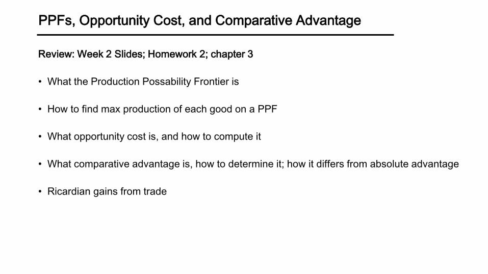
PPFs, Opportunity Cost, and Comparative Advantage
Review: Week 2 Slides; Homework 2; chapter 3
• What the Production Possability Frontier is
• How to find max production of each good on a PPF
• What opportunity cost is, and how to compute it
• What comparative advantage is, how to determine it; how it differs from absolute advantage
• Ricardian gains from trade
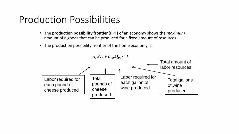
Production Possibilities• The production possibility frontier (PPF) of an economy shows the maximum
amount of a goods that can be produced for a fixed amount of resources.
• The production possibility frontier of the home economy is:
aLCQC + aLWQW ≤ L
Total gallons
of wine
produced
Labor required for
each pound of
cheese produced
Total
pounds of
cheese
produced
Labor required for
each gallon of
wine produced
Total amount of
labor resources
Production Possibilities (cont.)
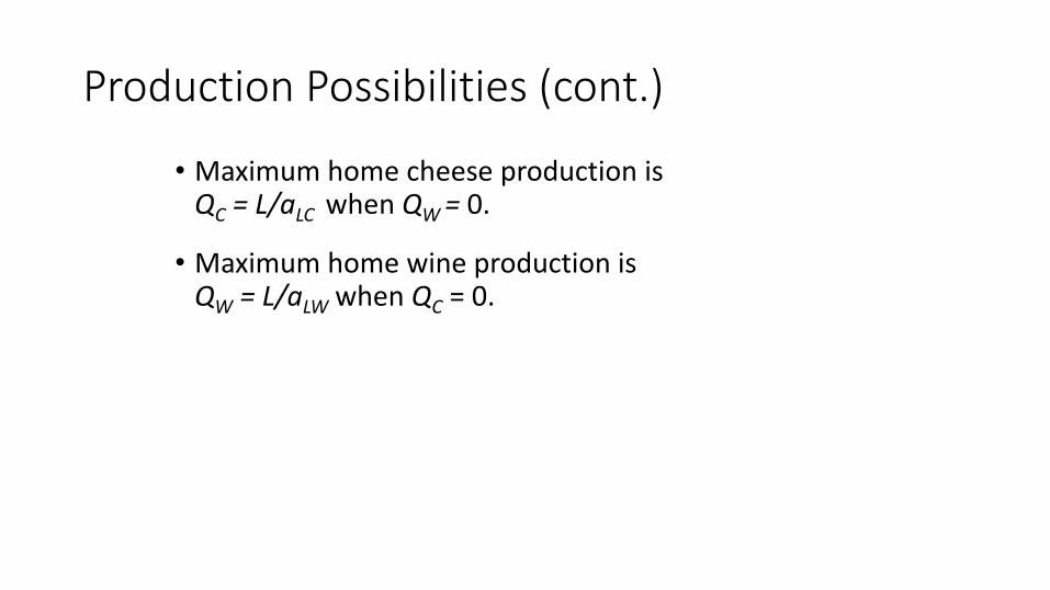
• Maximum home cheese production isQC = L/aLC when QW = 0.
• Maximum home wine production isQW = L/aLW when QC = 0.
Production Possibilities (cont.)
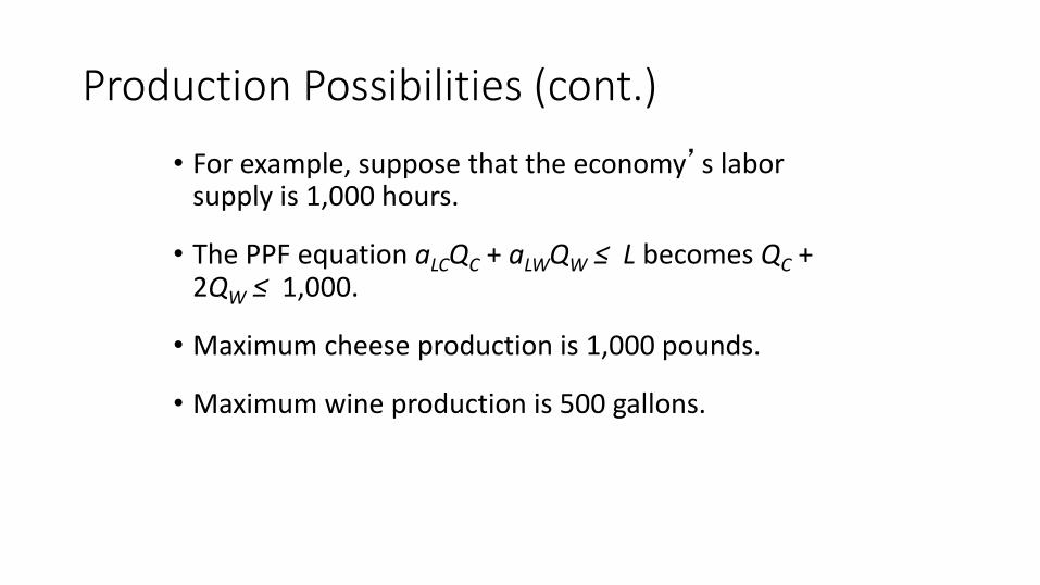
• For example, suppose that the economy’s labor supply is 1,000 hours.
• The PPF equation aLCQC + aLWQW ≤ L becomes QC + 2QW ≤ 1,000.
• Maximum cheese production is 1,000 pounds.
• Maximum wine production is 500 gallons.
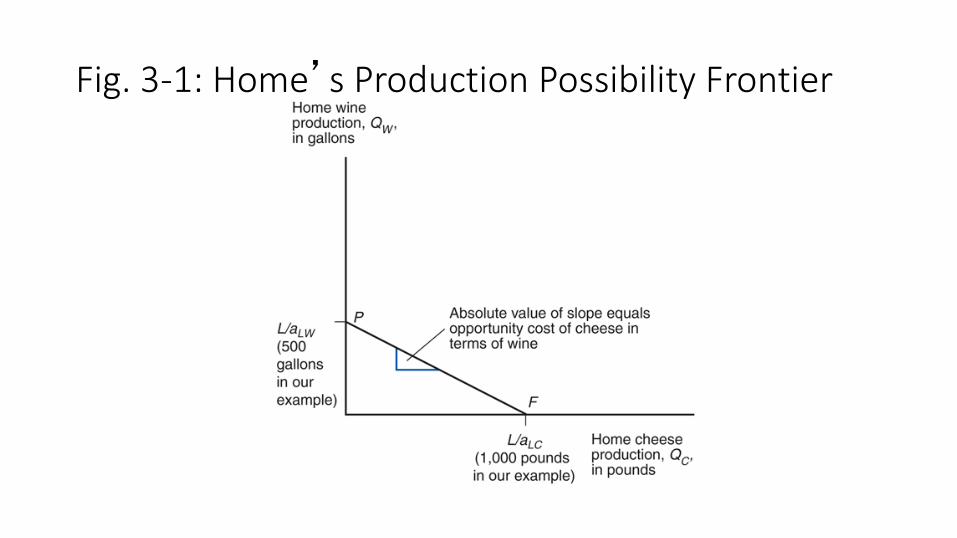
Fig. 3-1: Home’s Production Possibility Frontier
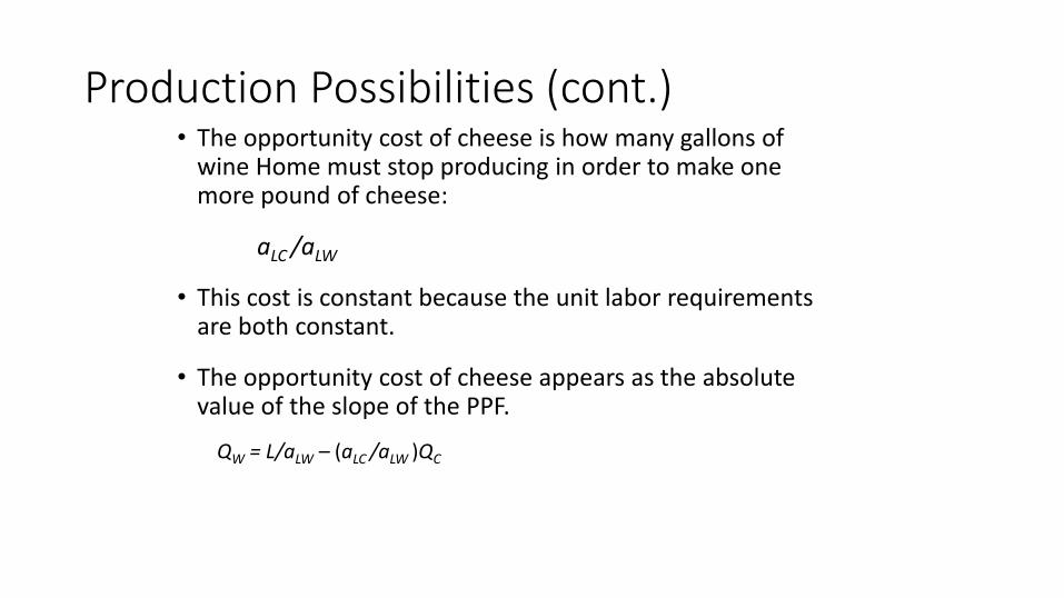
Production Possibilities (cont.)• The opportunity cost of cheese is how many gallons of
wine Home must stop producing in order to make one more pound of cheese:
aLC /aLW
• This cost is constant because the unit labor requirements are both constant.
• The opportunity cost of cheese appears as the absolute value of the slope of the PPF.
QW = L/aLW – (aLC /aLW )QC
Production Possibilities (cont.)
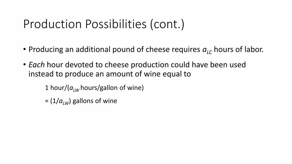
• Producing an additional pound of cheese requires aLC hours of labor.
• Each hour devoted to cheese production could have been used instead to produce an amount of wine equal to
1 hour/(aLW hours/gallon of wine)
= (1/aLW) gallons of wine
Production Possibilities (cont.)
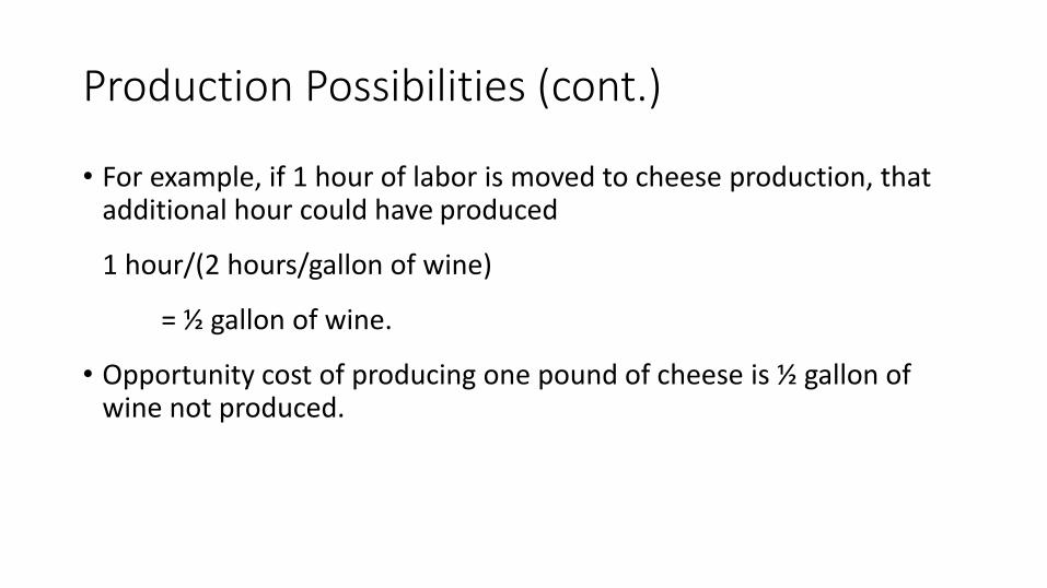
• For example, if 1 hour of labor is moved to cheese production, that additional hour could have produced
1 hour/(2 hours/gallon of wine)
= ½ gallon of wine.
• Opportunity cost of producing one pound of cheese is ½ gallon of wine not produced.
Homework Review: Comparative Advantage
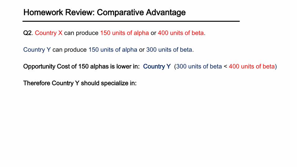
Q2. Country X can produce 150 units of alpha or 400 units of beta.
Country Y can produce 150 units of alpha or 300 units of beta.
Opportunity Cost of 150 alphas is lower in:
Therefore Country Y should specialize in:
Homework Review: Comparative Advantage
Q2. Country X can produce 150 units of alpha or 400 units of beta.
Country Y can produce 150 units of alpha or 300 units of beta.
Opportunity Cost of 150 alphas is lower in: Country Y (300 units of beta < 400 units of beta)
Therefore Country Y should specialize in:
Homework Review: Comparative Advantage
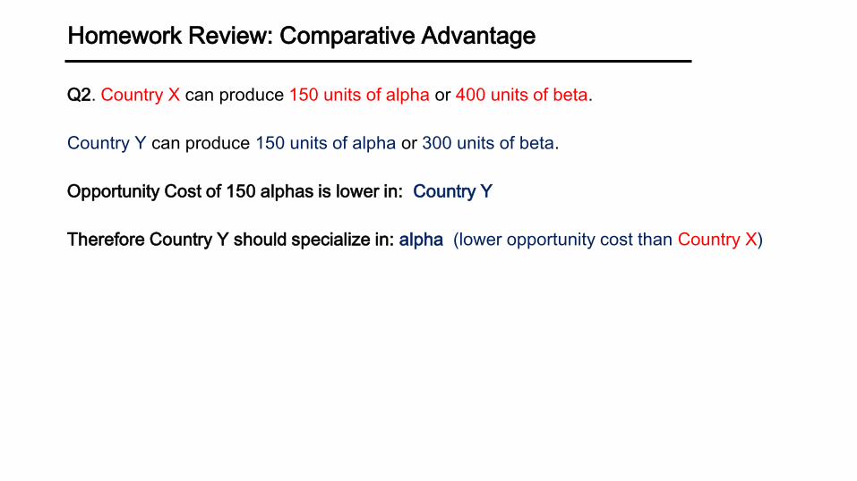
Q2. Country X can produce 150 units of alpha or 400 units of beta.
Country Y can produce 150 units of alpha or 300 units of beta.
Opportunity Cost of 150 alphas is lower in: Country Y
Therefore Country Y should specialize in: alpha (lower opportunity cost than Country X)
Homework Review: Comparative Advantage
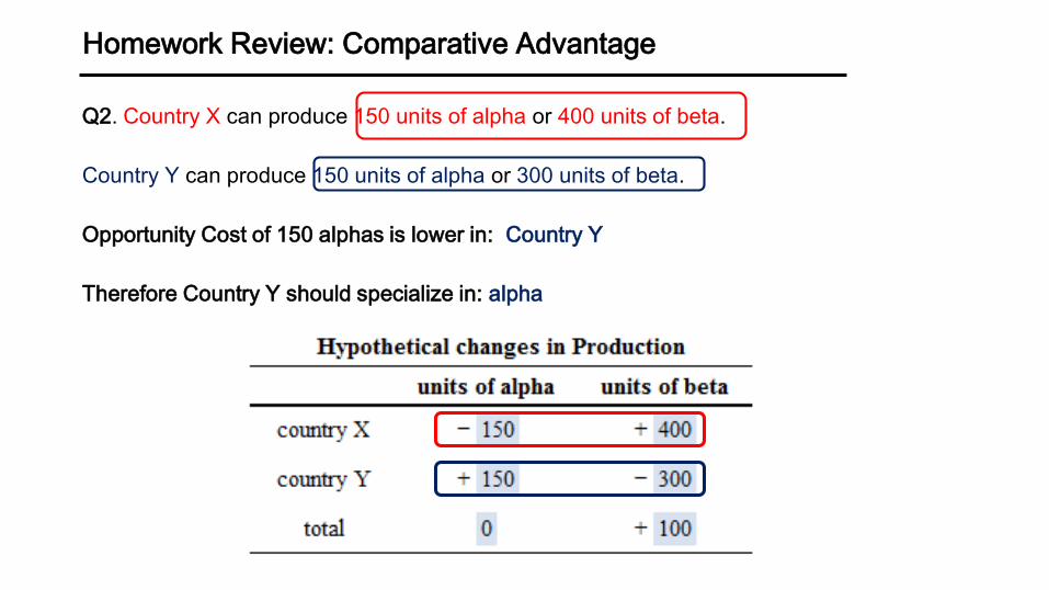
Q2. Country X can produce 150 units of alpha or 400 units of beta.
Country Y can produce 150 units of alpha or 300 units of beta.
Opportunity Cost of 150 alphas is lower in: Country Y
Therefore Country Y should specialize in: alpha
Homework Review: Comparative Advantage
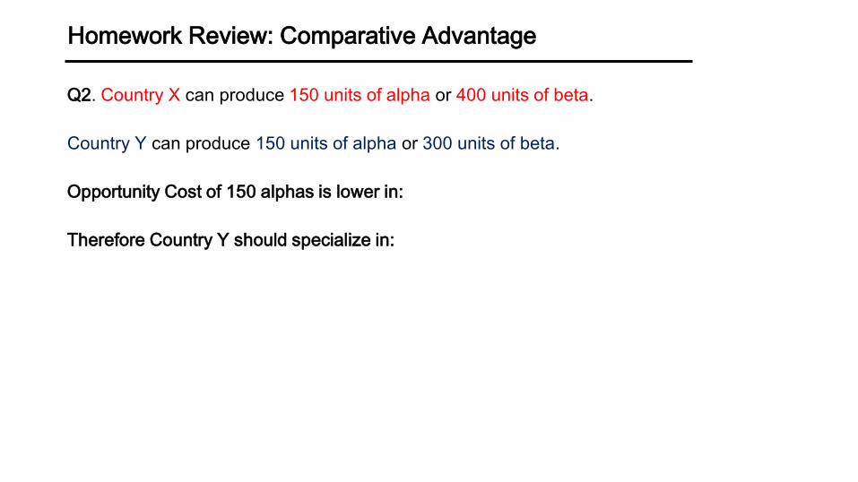
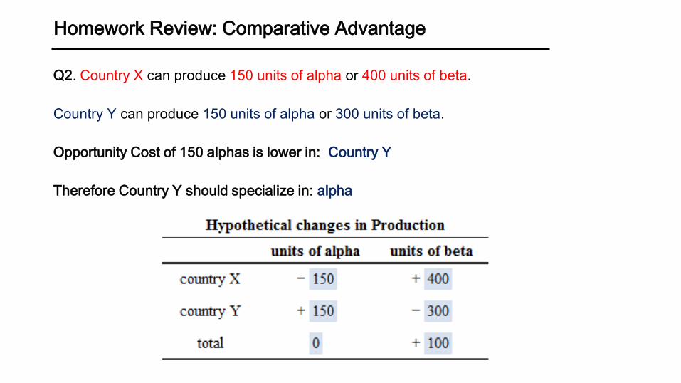
Q2. Country X can produce 150 units of alpha or 400 units of beta.
Country Y can produce 150 units of alpha or 300 units of beta.
Opportunity Cost of 150 alphas is lower in: Country Y
Therefore Country Y should specialize in: alpha

RS-RD, Relative Prices, Pattern of Specialization
Review: Week 2 Slides; Homework 2
• How relative supply and relative demand determine pattern of specialization
• How to use RS-RD graph to find equilibrium
• Pattern of Specialization
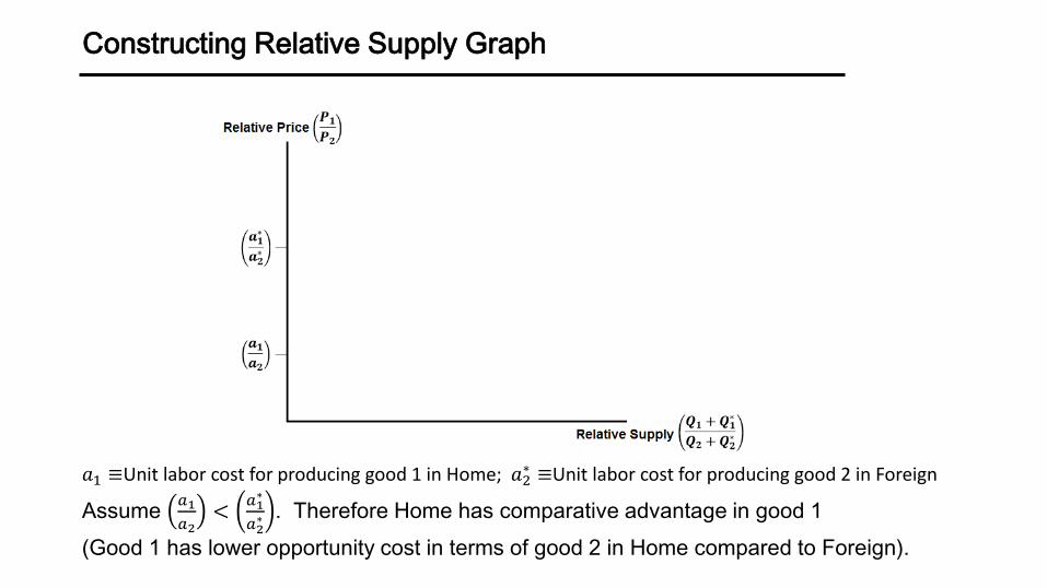
Constructing Relative Supply Graph
Assume 𝑎1
𝑎2<
𝑎1∗
𝑎2∗ . Therefore Home has comparative advantage in good 1
(Good 1 has lower opportunity cost in terms of good 2 in Home compared to Foreign).
𝑎1 ≡Unit labor cost for producing good 1 in Home; 𝑎2∗ ≡Unit labor cost for producing good 2 in Foreign
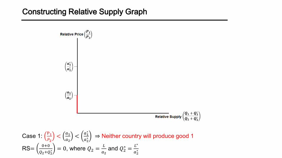
Constructing Relative Supply Graph
Case 1: P1
𝑃2<
𝑎1
𝑎2<
𝑎1∗
𝑎2∗ ⇒ Neither country will produce good 1
RS=0+0
𝑄2+𝑄2∗ = 0, where 𝑄2 =
𝐿
𝑎2and 𝑄2
∗ =𝐿∗
𝑎2∗
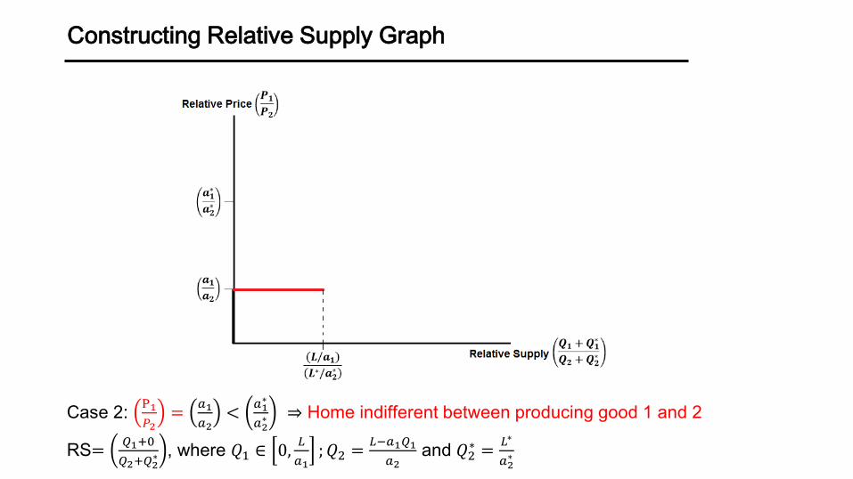
Constructing Relative Supply Graph
Case 2: P1
𝑃2=
𝑎1
𝑎2<
𝑎1∗
𝑎2∗ ⇒ Home indifferent between producing good 1 and 2
RS=𝑄1+0
𝑄2+𝑄2∗ , where 𝑄1 ∈ 0,
𝐿
𝑎1; 𝑄2 =
𝐿−𝑎1𝑄1
𝑎2and 𝑄2
∗ =𝐿∗
𝑎2∗
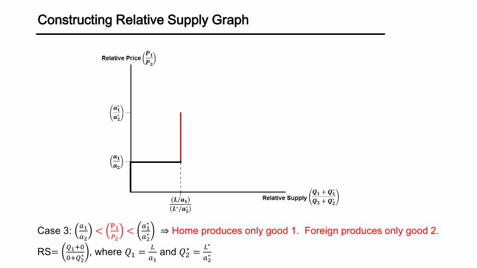
Constructing Relative Supply Graph
Case 3: 𝑎1
𝑎2<
P1
𝑃2<
𝑎1∗
𝑎2∗ ⇒ Home produces only good 1. Foreign produces only good 2.
RS=𝑄1+0
0+𝑄2∗ , where 𝑄1 =
𝐿
𝑎1and 𝑄2
∗ =𝐿∗
𝑎2∗
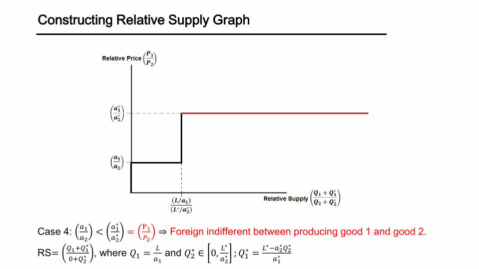
Constructing Relative Supply Graph
Case 4: 𝑎1
𝑎2<
𝑎1∗
𝑎2∗ =
P1
𝑃2⇒ Foreign indifferent between producing good 1 and good 2.
RS=𝑄1+𝑄1
∗
0+𝑄2∗ , where 𝑄1 =
𝐿
𝑎1and 𝑄2
∗ ∈ 0,𝐿∗
𝑎2∗ ; 𝑄1
∗ =𝐿∗−𝑎2
∗𝑄2∗
𝑎1∗
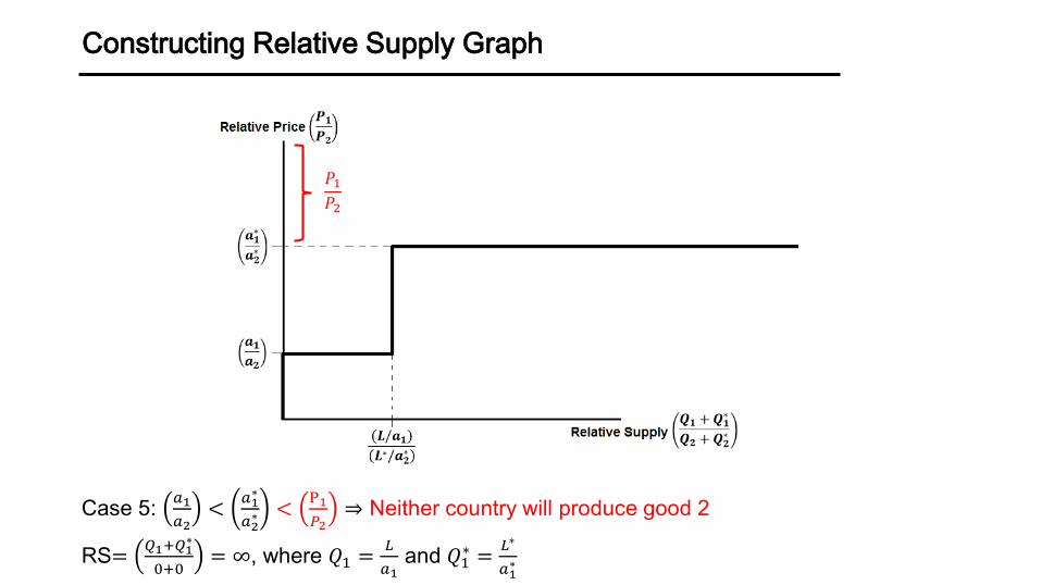
Constructing Relative Supply Graph
Case 5: 𝑎1
𝑎2<
𝑎1∗
𝑎2∗ <
P1
𝑃2⇒ Neither country will produce good 2
RS=𝑄1+𝑄1
∗
0+0= ∞, where 𝑄1 =
𝐿
𝑎1and 𝑄1
∗ =𝐿∗
𝑎1∗
𝑃1𝑃2
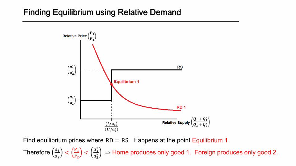
Finding Equilibrium using Relative Demand
Find equilibrium prices where RD = RS. Happens at the point Equilibrium 1.
Therefore 𝑎1
𝑎2<
P1
𝑃2<
𝑎1∗
𝑎2∗ ⇒ Home produces only good 1. Foreign produces only good 2.
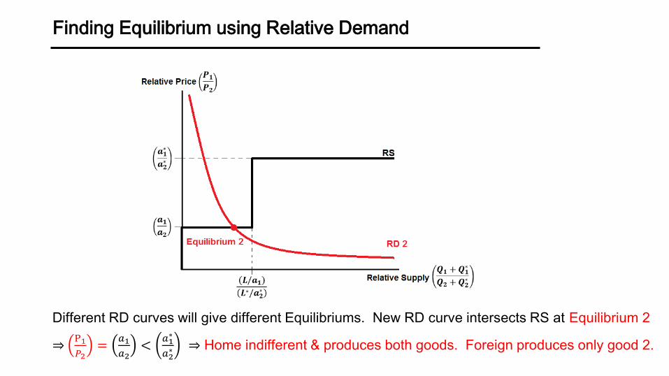
Finding Equilibrium using Relative Demand
Different RD curves will give different Equilibriums. New RD curve intersects RS at Equilibrium 2
⇒P1
𝑃2=
𝑎1
𝑎2<
𝑎1∗
𝑎2∗ ⇒ Home indifferent & produces both goods. Foreign produces only good 2.

Defining an Equilibrium
Review: Week 3 and 4 Slides, Worksheet 1, HW 3, PS1 Q1
• Endogeneous vs Exogeneous Paramters
• Monotonic transformations on Preferences (OK) vs Production Functions (not OK)
• Basic idea of Walras‘ Law.
How to define a competitive equilibrium
• Consumer‘s problem (Max utility subject to Budget Constraint)
• Firm‘s problem (Max Profits subject to production technology)
• Market Clearing for Goods and Labor
Example of Utility function
Let there be two goods: 𝑐1 is consumption of good 1, 𝑐2 is consumption of good 2.
• Cobb-Douglas Utility Function:
𝑈 𝑐1, 𝑐2 = 𝑐1𝜃1 𝑐2
𝜃2
Important: Utility doesn‘t have natural units. Only relative utility matters.
• Transformations that preserve ordering are considered equivalent utility functions.
• Common order preserving transofrmations: Addition, Multiplication, Powers, Logairthms
Example Transformation: Take logarithm
𝑈 𝑐1, 𝑐2 = 𝜃1 log 𝑐1 + 𝜃2 log 𝑐2
𝑈 𝑐1, 𝑐2 is the same utility function as 𝑈 𝑐1, 𝑐2 [Note log 0 = −∞, always consume some of both]
Consumer Problem
Consumer problem will be to maximize utility function, subject to budget constraint
Budget Constraint
• Without a budget constraint, consumers would want an infinite amount of everything
• Budget constraint enforces that consumer expenditures are less than consumer income
• Typically no borrowing or saving in this class (we focus mainly on static models)
Consumption Expenditures: Sum of expenditures (= price * quantity) across all goods.
Income Sources: Labor income (wages * labor supplied).
Other potential sources: rental rates from capital, profits from firms, taxes from government
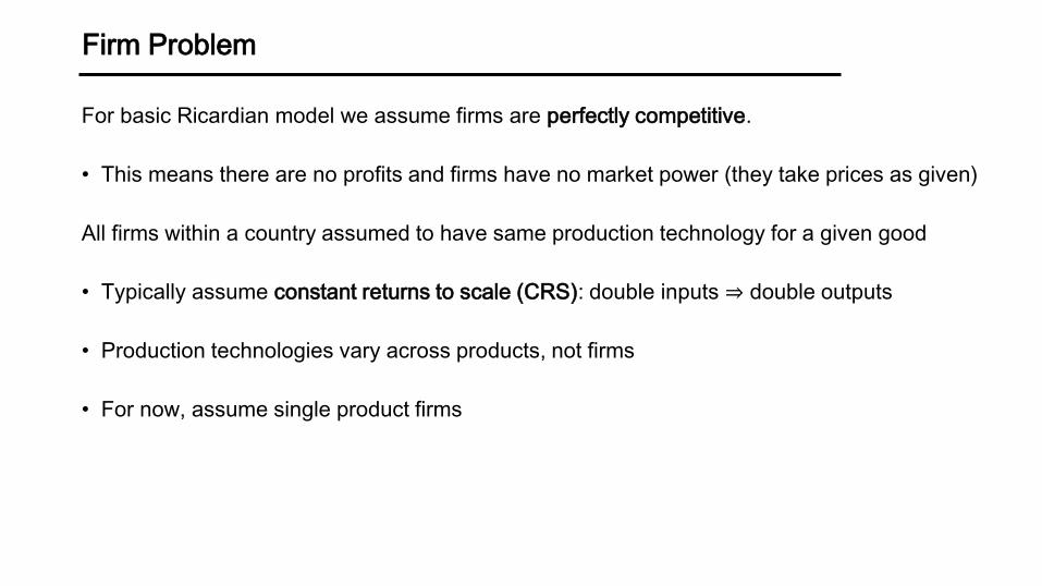
Firm Problem
For basic Ricardian model we assume firms are perfectly competitive.
• This means there are no profits and firms have no market power (they take prices as given)
All firms within a country assumed to have same production technology for a given good
• Typically assume constant returns to scale (CRS): double inputs ⇒ double outputs
• Production technologies vary across products, not firms
• For now, assume single product firms
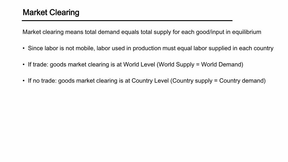
Market Clearing
Market clearing means total demand equals total supply for each good/input in equilibrium
• Since labor is not mobile, labor used in production must equal labor supplied in each country
• If trade: goods market clearing is at World Level (World Supply = World Demand)
• If no trade: goods market clearing is at Country Level (Country supply = Country demand)

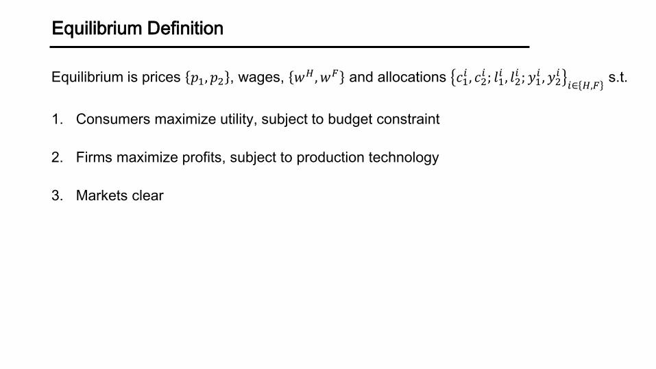
Equilibrium Definition
Equilibrium is prices 𝑝1, 𝑝2 , wages, 𝑤𝐻 , 𝑤𝐹 and allocations 𝑐1𝑖 , 𝑐2𝑖 ; 𝑙1𝑖 , 𝑙2𝑖 ; 𝑦1
𝑖 , 𝑦2𝑖𝑖∈ 𝐻,𝐹
s.t.
1. Consumers maximize utility, subject to budget constraint
2. Firms maximize profits, subject to production technology
3. Markets clear
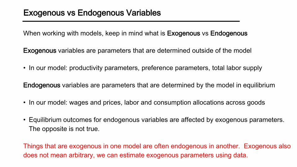
Exogenous vs Endogenous Variables
When working with models, keep in mind what is Exogenous vs Endogenous
Exogenous variables are parameters that are determined outside of the model
• In our model: productivity parameters, preference parameters, total labor supply
Endogenous variables are parameters that are determined by the model in equilibrium
• In our model: wages and prices, labor and consumption allocations across goods
• Equilibrium outcomes for endogenous variables are affected by exogenous parameters.
The opposite is not true.
Things that are exogenous in one model are often endogenous in another. Exogenous also
does not mean arbitrary, we can estimate exogenous parameters using data.
Equilibrium Definition
Equilibrium is prices 𝑝1, 𝑝2 , wages, 𝑤𝐻 , 𝑤𝐹 and allocations 𝑐1𝑖 , 𝑐2𝑖 ; 𝑙1𝑖 , 𝑙2𝑖 ; 𝑦1
𝑖 , 𝑦2𝑖𝑖∈ 𝐻,𝐹
s.t.
1. Consumers maximize utility, subject to budget constraint
2. Firms maximize profits, subject to production technology
3. Markets clear
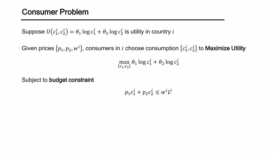
Consumer Problem
Suppose 𝑈 𝑐1𝑖 , 𝑐2𝑖 = 𝜃1 log 𝑐1
𝑖 + 𝜃2 log 𝑐2𝑖 is utility in country 𝑖
Given prices 𝑝1, 𝑝2, 𝑤𝑖 , consumers in 𝑖 choose consumption 𝑐1
𝑖 , 𝑐2𝑖 to Maximize Utility
max𝑐1,𝑐2
𝜃1 log 𝑐1𝑖 + 𝜃2 log 𝑐2
𝑖
Subject to budget constraint
𝑝1𝑐1𝑖 + 𝑝2𝑐2
𝑖 ≤ 𝑤𝑖𝐿𝑖
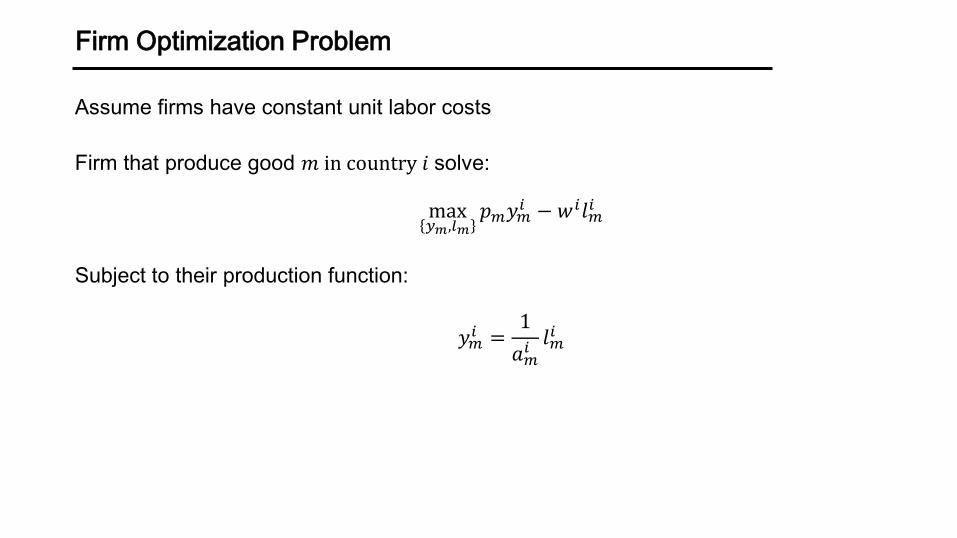
Firm Optimization Problem
Assume firms have constant unit labor costs
Firm that produce good 𝑚 in country 𝑖 solve:
max𝑦𝑚,𝑙𝑚
𝑝𝑚𝑦𝑚𝑖 − 𝑤𝑖𝑙𝑚
𝑖
Subject to their production function:
𝑦𝑚𝑖 =
1
𝑎𝑚𝑖𝑙𝑚𝑖
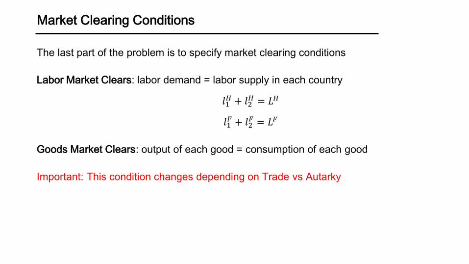
Market Clearing Conditions
The last part of the problem is to specify market clearing conditions
Labor Market Clears: labor demand = labor supply in each country
𝑙1𝐻 + 𝑙2
𝐻 = 𝐿𝐻
𝑙1𝐹 + 𝑙2
𝐹 = 𝐿𝐹
Goods Market Clears: output of each good = consumption of each good
Important: This condition changes depending on Trade vs Autarky
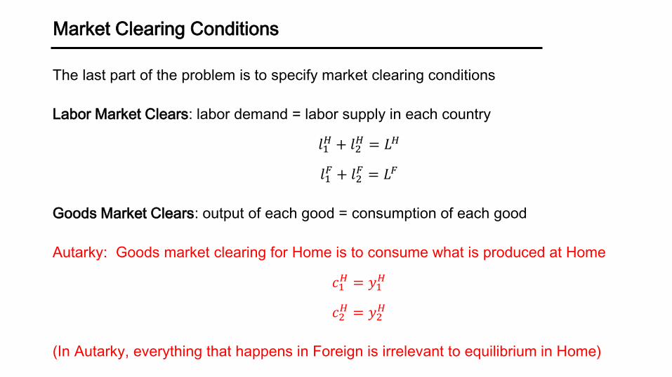
Market Clearing Conditions
The last part of the problem is to specify market clearing conditions
Labor Market Clears: labor demand = labor supply in each country
𝑙1𝐻 + 𝑙2
𝐻 = 𝐿𝐻
𝑙1𝐹 + 𝑙2
𝐹 = 𝐿𝐹
Goods Market Clears: output of each good = consumption of each good
Autarky: Goods market clearing for Home is to consume what is produced at Home
𝑐1𝐻 = 𝑦1
𝐻
𝑐2𝐻 = 𝑦2
𝐻
(In Autarky, everything that happens in Foreign is irrelevant to equilibrium in Home)
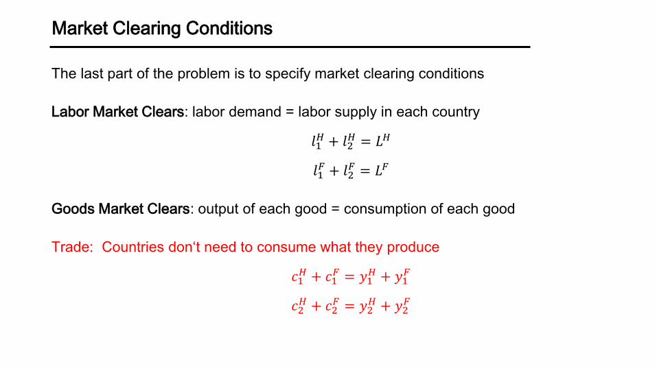
Market Clearing Conditions
The last part of the problem is to specify market clearing conditions
Labor Market Clears: labor demand = labor supply in each country
𝑙1𝐻 + 𝑙2
𝐻 = 𝐿𝐻
𝑙1𝐹 + 𝑙2
𝐹 = 𝐿𝐹
Goods Market Clears: output of each good = consumption of each good
Trade: Countries don‘t need to consume what they produce
𝑐1𝐻 + 𝑐1
𝐹 = 𝑦1𝐻 + 𝑦1
𝐹
𝑐2𝐻 + 𝑐2
𝐹 = 𝑦2𝐻 + 𝑦2
𝐹

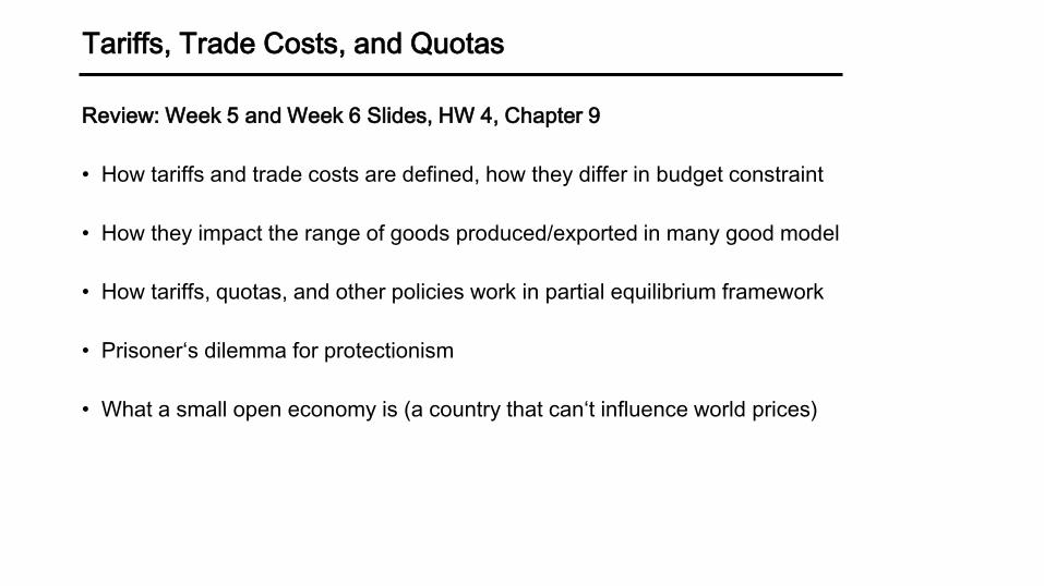
Tariffs, Trade Costs, and Quotas
Review: Week 5 and Week 6 Slides, HW 4, Chapter 9
• How tariffs and trade costs are defined, how they differ in budget constraint
• How they impact the range of goods produced/exported in many good model
• How tariffs, quotas, and other policies work in partial equilibrium framework
• Prisoner‘s dilemma for protectionism
• What a small open economy is (a country that can‘t influence world prices)
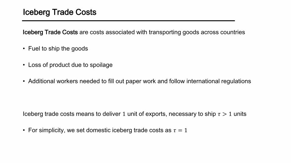
Iceberg Trade Costs
Iceberg Trade Costs are costs associated with transporting goods across countries
• Fuel to ship the goods
• Loss of product due to spoilage
• Additional workers needed to fill out paper work and follow international regulations
Iceberg trade costs means to deliver 1 unit of exports, necessary to ship 𝜏 > 1 units
• For simplicity, we set domestic iceberg trade costs as 𝜏 = 1
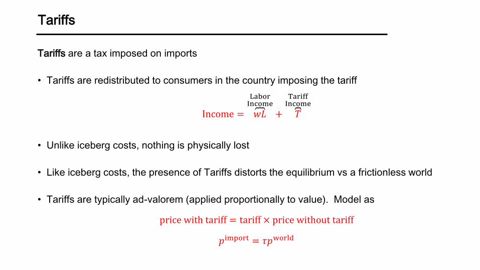
Tariffs
Tariffs are a tax imposed on imports
• Tariffs are redistributed to consumers in the country imposing the tariff
Income = 𝑤𝐿
LaborIncome
+ 𝑇
TariffIncome
• Unlike iceberg costs, nothing is physically lost
• Like iceberg costs, the presence of Tariffs distorts the equilibrium vs a frictionless world
• Tariffs are typically ad-valorem (applied proportionally to value). Model as
price with tariff = tariff × price without tariff
𝑝import = 𝜏𝑝world
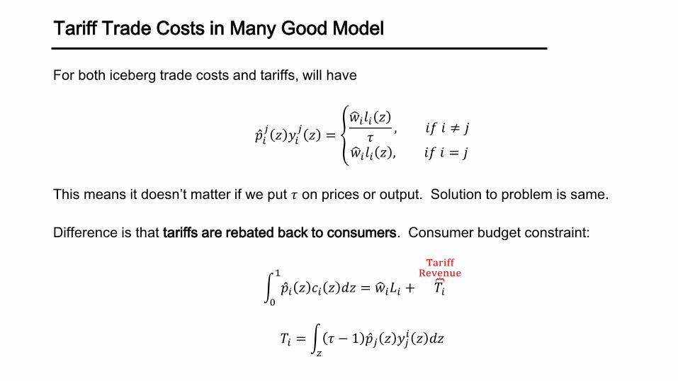
Tariff Trade Costs in Many Good Model
For both iceberg trade costs and tariffs, will have
𝑝𝑖𝑗𝑧 𝑦𝑖
𝑗𝑧 =
𝑤𝑖𝑙𝑖 𝑧
𝜏, 𝑖𝑓 𝑖 ≠ 𝑗
𝑤𝑖𝑙𝑖 𝑧 , 𝑖𝑓 𝑖 = 𝑗
This means it doesn’t matter if we put 𝜏 on prices or output. Solution to problem is same.
Difference is that tariffs are rebated back to consumers. Consumer budget constraint:
0
1
𝑝𝑖 𝑧 𝑐𝑖 𝑧 𝑑𝑧 = 𝑤𝑖𝐿𝑖 + 𝑇𝑖
TariffRevenue
𝑇𝑖 = 𝑧
𝜏 − 1 𝑝𝑗 𝑧 𝑦𝑗𝑖 𝑧 𝑑𝑧
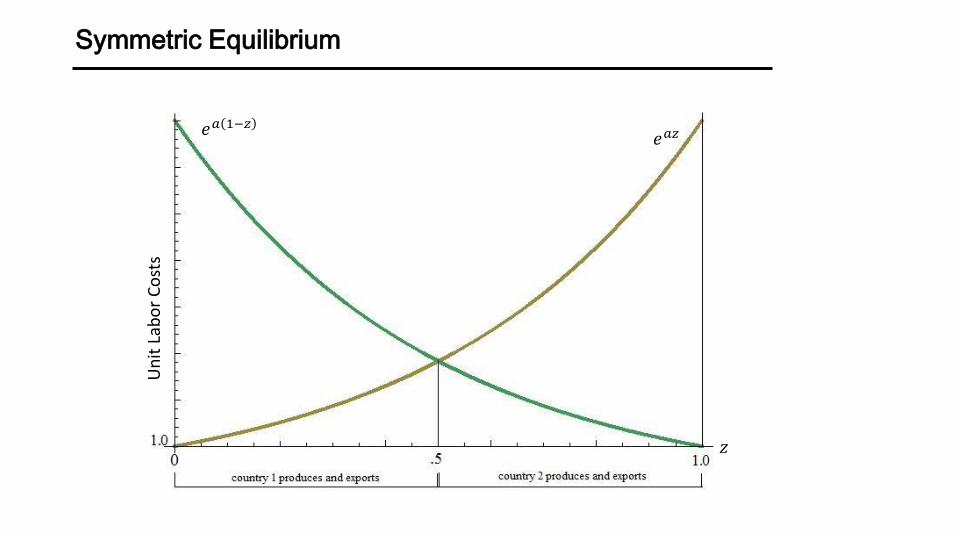
Symmetric Equilibrium
𝑒𝑎𝑧𝑒𝑎 1−𝑧
Un
it L
abo
r C
ost
s
𝑧
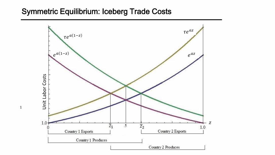
Symmetric Equilibrium: Iceberg Trade Costs
𝜏𝑒𝑎 1−𝑧
𝑧
𝑒𝑎 1−𝑧
𝜏𝑒𝑎𝑧
𝑒𝑎𝑧
Un
it L
abo
r C
ost
s
1
Instruments of Trade Policy
Many instruments available to affect international trade flows and prices. Non-exhaustive list:
• Tariffs: Taxes on Imports. Effect is to increase price of imports, decrease quantity of imports,
and collect tariff revenues.
• Export Subsidies: Subsidies on exports. Effect is to decrease price of exports and increase
quantity of exports. Must be funded by government.
• Quotas: Limits on quantity of imports. Effect is to increase price of imports, decrease quantity of
imports.
• Export Restrictions: Limits on quantity of exports. Effect is to increase price of exports, decrease
quantity of exports.
• Local Content Requirements: Requirement that a sufficient portion of value added for a good is
local. Increases price of imports (due to higher production costs), and decreases quantity.
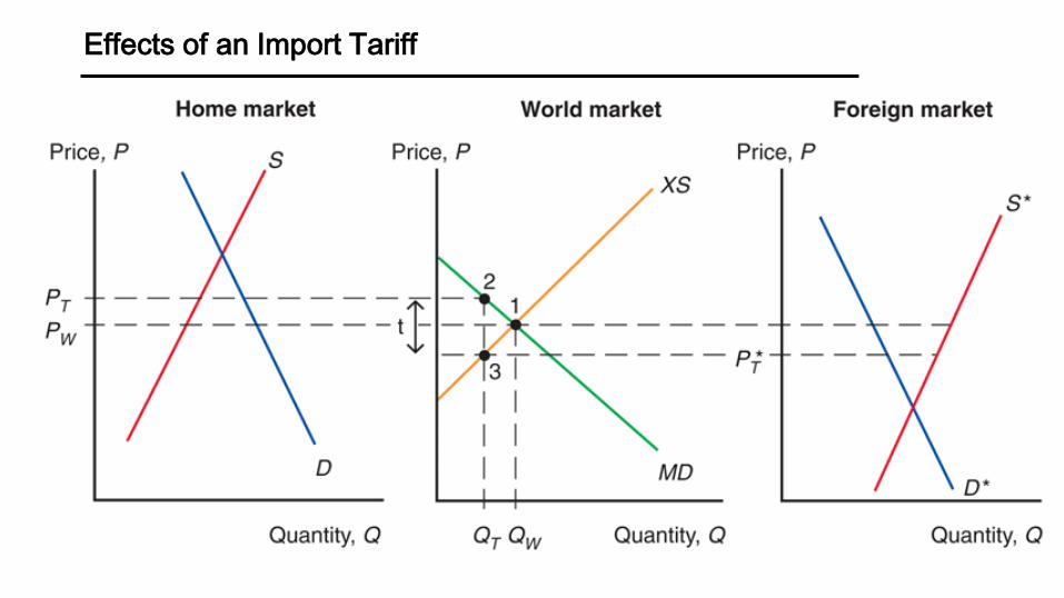
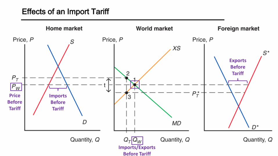
Effects of an Import Tariff
Effects of an Import Tariff
ImportsBeforeTariff
ExportsBeforeTariff
Imports/ExportsBefore Tariff
PriceBeforeTariff
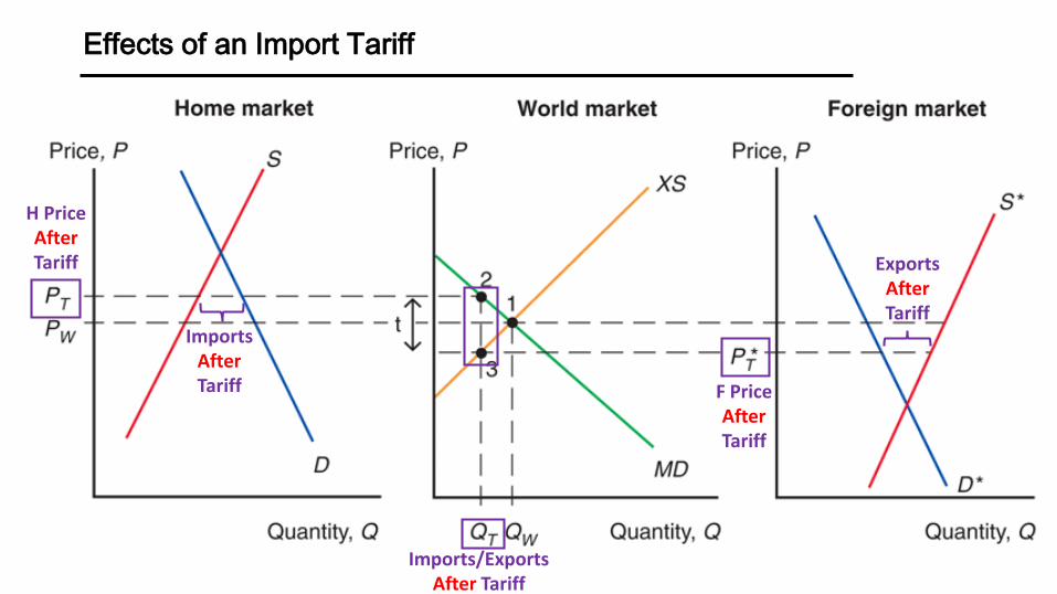
Effects of an Import Tariff
ImportsAfterTariff
ExportsAfterTariff
Imports/ExportsAfter Tariff
H PriceAfterTariff
F PriceAfterTariff
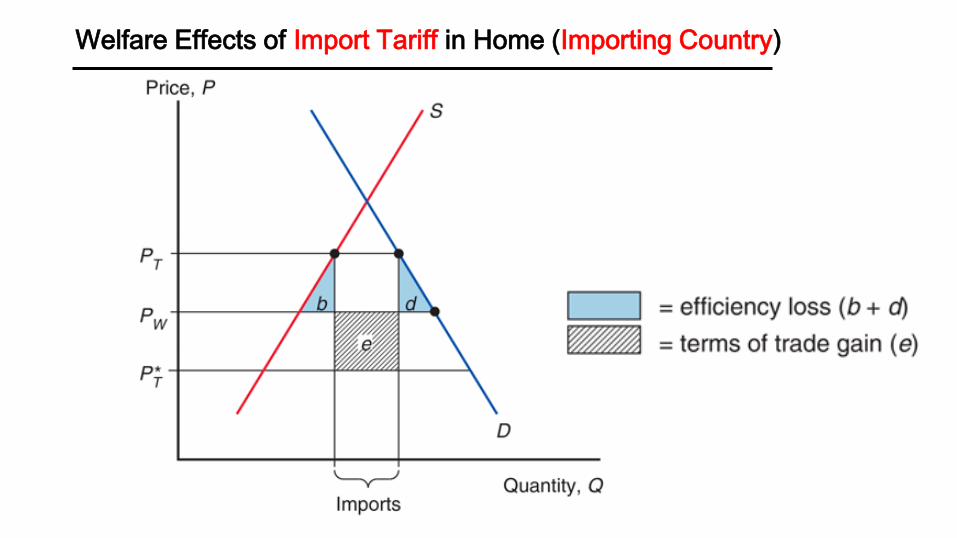
Welfare Effects of Import Tariff in Home (Importing Country)
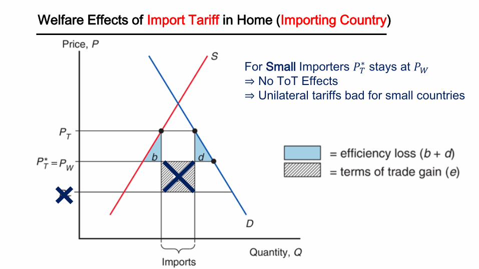
Welfare Effects of Import Tariff in Home (Importing Country)
For Small Importers 𝑃𝑇∗ stays at 𝑃𝑊
⇒ No ToT Effects
⇒ Unilateral tariffs bad for small countries
=
Effects of an Import Quota
Import Quotas restict quantity of imports
• Quotas typically enforced by issueing licenses to exporters
• Owners of quota licenses have market power, and can earn quota rents
• In practice, Government may choose to sell quota licenses. This allows government to capture
quota rents, and the quota then acts like a tariff.
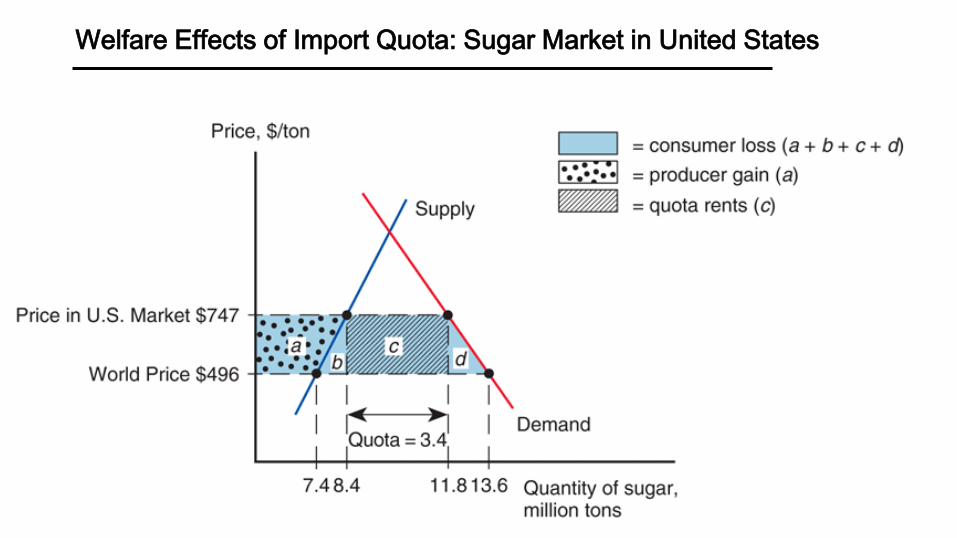
Welfare Effects of Import Quota: Sugar Market in United States


![POLICY PARTNERSHIP ON FOOD SECURITY (PPFS) APEC FOOD ... · APEC Policy Partnership on Food Security [PPFS], as primary mechanism for APEC economies to address food security issues,is](https://img.pdfslide.us/doc/110x75/5fee453683ea9127795ac612/policy-partnership-on-food-security-ppfs-apec-food-apec-policy-partnership.jpg)