ECMWF short-range forecast errors · 2007-08-17 · and mixed Rossby gravity(MRG) modes (Matsuno 1966). Indeed, equatorially trapped Kelvin, MRG and equatorial IG (EIG) waves have

Q. J. R. Meteorol. Soc. (2005), 131, pp. 987–1011 doi: 10.1256/qj.04.54

Balanced tropical data assimilation based on a study of equatorial waves inECMWF short-range forecast errors

By NEDJELJKA ZAGAR1∗, ERIK ANDERSSON2 and MICHAEL FISHER2

1Stockholm University, Sweden2European Centre for Medium-Range Weather Forecasts, Reading, UK

(Received 2 April 2004; revised 25 November 2004)

SUMMARY

This paper seeks to represent the tropical short-range forecast error covariances of the European Centre forMedium-Range Weather Forecasts (ECMWF) model in terms of equatorial waves. The motivation for undertakingthis investigation is increasing observational evidence indicating that a substantial fraction of the tropical large-scale variability can be explained by equatorially trapped wave solutions known from shallow-water theory. Short-range forecast differences from a data-assimilation ensemble were taken to serve as a proxy for background errors.

It was found that the equatorial waves coupled to convection can explain on average 60–70% of the errorvariance in the tropical free atmosphere. The largest part of this explained variance is represented by the equatorialRossby (ER) modes, and a significant percentage pertains to the equatorial inertio-gravity (EIG) modes. Eastward-propagating EIG modes have maximum variance in the stratosphere, where the short-wave variance in westward-moving waves is particularly small. This feature is most likely related to the phase of the quasi-biennial oscillationduring the study period, suggesting that significant temporal variations could be present in longer-term time seriesof such statistics.

The vertical correlations for ER modes display characteristics similar to those of their extratropical coun-terparts: correlations narrow towards shorter scales and in the stratosphere. However, the present statistics donot display the significant increase with altitude of the horizontal correlation scale for the height field which istypical for global, quasi-geostrophic statistics commonly used in current data-assimilation schemes. Furthermore,tropospheric ER correlations are vertically asymmetric and deeper for the n = 1 mode than for higher modes. Mostlikely, deep convection, acting as a generator of equatorial wave motion, is the dominant mechanism underlyingthese results.

In spite of its relatively small contribution to the tropospheric variance, the Kelvin-wave coupling plays adecisive role for determining the characteristics of the horizontal correlation near the equator. EIG modes alsoplay an important role for the tropical mass–wind coupling; these waves have a major impact by reducing themeridional correlation scales and the magnitudes of the balanced height-field increments.

KEYWORDS: Covariance modelling Ensemble methods Mass–wind coupling Tropics Variationaldata assimilation

1. INTRODUCTION

Numerical weather-prediction (NWP) models are never going to be error-free.A reliable estimate of their forecast errors poses a real challenge, since the knowledgeof the true state of the atmosphere is beyond our grasp. In data assimilation for NWP,short-range forecast errors are commonly referred to as background errors; they arefrequently represented by surrogate quantities with statistical and dynamical propertiesassumed similar to those of the unknown forecast errors (e.g. Parrish and Derber 1992).Derived dependencies are built into the background-error covariance matrix for dataassimilation; the purpose of these relationships is to spread observed information froma point to nearby grid points and levels. Moreover, the observed information is alsodistributed to other variables. In this way observations of the temperature field carryinformation about the wind field, and vice versa. This is the fundamental reason why thebalance relationships between the mass- and the wind-field variables are of such greatimportance for data assimilation, especially in regions where observations are sparseand in a Global Observing System (GOS) dominated by mass-field information.

∗ Corresponding author: Department of Meteorology, Stockholm University, SE-106 91 Stockholm, Sweden.e-mail: [email protected]© Royal Meteorological Society, 2005.

987

988 N. ZAGAR et al.

In the midlatitudes, the basic balance relationship is geostrophy, which has beenextensively used in analysis procedures (e.g. Courtier et al. 1998; Gustafsson et al.2001). The most important elements of atmospheric motion are Rossby waves; theiraccurate analysis is, therefore, the primary concern in data assimilation for NWP. Toensure that the observational information is assimilated mainly in terms of Rossbymodes, initialization procedures and methods for generating geostrophically balancedincrements have been developed. As a result, the excessive generation of inertio-gravity(IG) waves is suppressed.

In the tropics, on the other hand, a dominant relationship similar to geostrophyis lacking; the analysis here has thus traditionally been undertaken in the univariatefashion. Consequently, large-scale divergence fields, such as the Hadley and Brewer–Dobson circulations, are analysed nearly univariately. Since GOS in the tropics relieson mass-field information, uncertainties in the analysed wind field are significant (e.g.Kistler et al. 2001). Furthermore, large-scale motion in the tropics cannot be consideredwithout taking into account IG waves (e.g. Browning et al. 2000). In addition, the changeof sign of the Coriolis parameter, f , at the equator gives rise to important types of large-scale non-rotational motion, which are absent in the midlatitude atmosphere: the Kelvinand mixed Rossby–gravity (MRG) modes (Matsuno 1966).

Indeed, equatorially trapped Kelvin, MRG and equatorial IG (EIG) waves haveregularly been detected in observations since the 1960s. Recent observational studies(Wheeler and Kiladis 1999; Yang et al. 2003) identified equatorially trapped wavestructures in long-term satellite observations of outgoing long-wave radiation, a proxyfor deep tropical cloudiness. The waves have been denoted the ‘convectively-coupledequatorial waves’, as their presence in areas of moist convection implies an interactionbetween convection and the dynamics. This causes the wave characteristics to change:their frequency is lowered, i.e. the equivalent depth is becoming smaller. Availableequivalent-depth estimates according to linear shallow-water theory are in the range 12–50 m (Wheeler and Kiladis 1999, and references therein). These observational studiesthus corroborate an earlier numerical model study by Ko et al. (1989), which revealedthat ‘the gravity waves associated with the shallow vertical modes and long zonal wavesplay an important role in the balanced gravitational energy’. Normal-mode-based 3D-Var and initialization techniques (Cats and Wergen 1983; Wergen 1988; Heckley et al.1992; Andersson et al. 1998) have therefore been unsuccessful in the tropics.

In the present study we consider Kelvin, MRG and EIG waves, in addition toequatorial Rossby (ER) modes, as balanced tropical motion, and investigate the extent towhich these equatorially trapped wave solutions are present in the ECMWF (EuropeanCentre for Medium-Range Weather Forecasts) short-range forecast errors. An ultimategoal is to construct a background-error covariance matrix comprising the couplingbetween the mass and the wind field in the tropics.

In the background-error modelling, an important, commonly made, assumptionis that the forecast errors are dominated by the balances of the model’s slow modes(Phillips 1986); this implies that background-error covariances are dominated by struc-tures similar to that of growing quasi-geostrophic perturbations in a model atmosphere.In accordance with these assumptions, we employ equatorial-wave theory to replacethe quasi-geostrophic relationships that have proven to be successful in extratropicallatitudes. The idea has previously been presented in Zagar et al. (2004, henceforthZGK), summarized here in section 2. This section also describes a data-assimilationensemble, used to extract short-range forecast differences to serve as a proxy for back-ground errors; the justification is given in the appendix. We investigate how accuratelya spectral, mode-based covariance model can represent the dominant characteristics of

BALANCED TROPICAL DATA ASSIMILATION 989

the ECMWF short-range tropical forecast errors. The resulting covariance statistics arepresented in section 3. In section 4, the covariance model is implemented in the vari-ational data-assimilation scheme developed in ZGK and utilized for an examinationof horizontal structures in the troposphere and stratosphere through idealized single-observation experiments. Conclusions are presented in section 5.

2. BACKGROUND-ERROR COVARIANCE MODELLING FOR THE TROPICS

(a) An ensemble-based datasetThe current background-error covariance model in operational use within the 4D-

Var system at ECMWF (Fisher 2003) is based on statistics of concurrent short-rangeforecast differences between members of a data-assimilation ensemble. The justificationfor this approach is given in the appendix. The ensemble consists of ten independentdata assimilations that each use different sets of randomly perturbed observationsover a period of 31 days in October 2000. For the purposes of this study, forecastdifferences were extracted from the ensemble, for the tropical belt 20◦S−20◦N, whichis commonly used in observational studies. A one-degree resolution is used in bothhorizontal directions. The two wind components and geopotential height were availableat 60 model levels, for different forecast lengths: 3-, 12- and 24-hour forecasts havebeen used. The results presented here are with respect to 12-hour forecast errors, but theoutputs for other ranges are very similar.

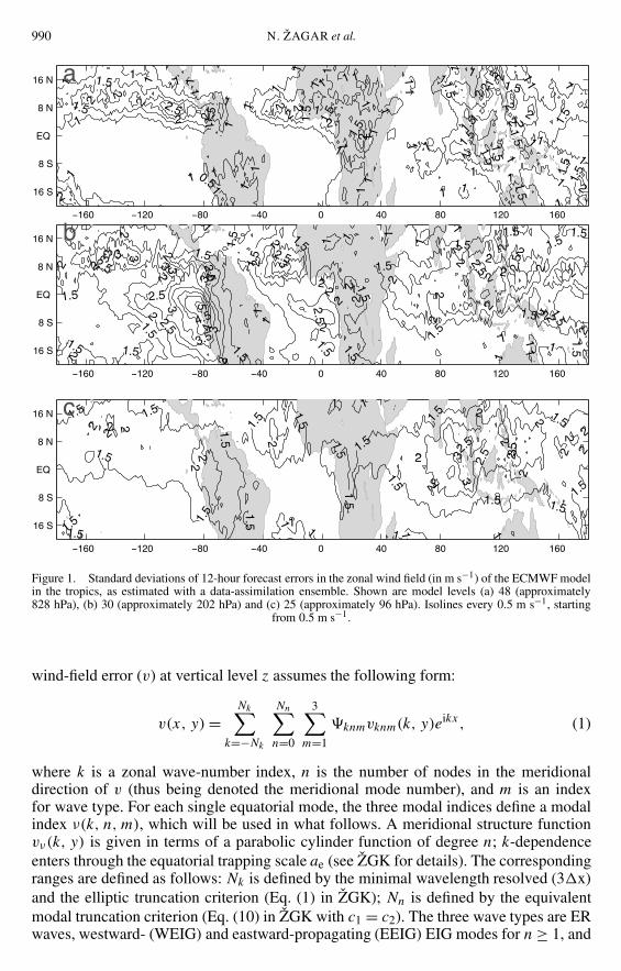
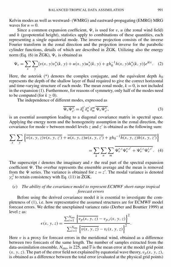
The ensemble standard deviation of error for the zonal wind is shown in Fig. 1at three model levels: in the lower and upper troposphere and near the tropopause.A striking feature in the lower troposphere is the frequent occurrence of errors alongthe intertropical convergence zone (ITCZ) and over Indonesia (Fig. 1(a)). Local maximaare located west of the tropical continents. The absolute error maximum is found in theupper troposphere, near the 200 hPa level, just west of South America (Fig. 1(b)). Higherup, the Indonesian region displays larger errors than the rest of the domain (Fig. 1(c)),whereas above the tropopause the errors become largely homogeneous.

The errors in the meridional wind field display a similar structure in the lowertroposphere (not shown), but higher up the error maxima near the South American coastand over Indonesia are weaker (up to 50 %) and the errors become more homogeneous atlower altitude as compared to the zonal wind errors. Errors in geopotential (not shown)are larger over the continents than over the oceans in the lower troposphere, with peaksassociated with orographic features. There is an error maximum over Indonesia in theupper troposphere, but above the tropopause the spatial error variations become small.

Figure 1 shows standard deviations of 12-hour forecast errors; however, patternsand magnitudes are similar for the other ranges (3 and 24 hours). The wind-field errorsgrow in time, at least in the troposphere. The growth is larger during the later 12-hourperiod (12–24 hours), and it is largest for levels between 100 and 300 hPa. Areas oflargest error growth coincide with the areas of significant error in Fig. 1, i.e. the largesterrors are located just west of South America between levels 28 (154 hPa) and 35(353 hPa). The geopotential-error growth is almost negligible. The stratospheric forecasterrors do not grow during 24 hours: on the contrary, they are on average 2% smaller thanthe 3-hour errors for all fields.

(b) Covariance-model formulationIn the present study, forecast errors are represented in terms of tropical eigenmodes

based on a parabolic cylinder function expansion. The expansion for the meridional

990 N. ZAGAR et al.

160 120 80 40 0 40 80 120 160

16 S

8 S

EQ

8 N

16 N

0.5

11

11

11

1

1

1

1

1

1

11

1 1

1

11

1

1

1

1

11

1

1

1

1

1

11

1

1

1

1

1

1

1

11

11

111

1

1

1

11

1

1

1 1.5

1.5

1.51.5

1.5

1.5

1.5

1.51.5

1.5

1.5

1.51.5

1.51.

51.5

1.51.

5

22

2

2

2222

22

222

2

2

2

2

2

2

2

2.5

a

160 120 80 40 0 40 80 120 160

16 S

8 S

EQ

8 N

16 N

1

1

1

1

1

11

1

1

11

111.5 1.5

1.5

1.5

1.5

1.5

1.5

1.5

1.5

1.5

1.5

1.5

1.5

1.5

1.5

1.5

1.51.5

1.5

1.5

1.52

2

2

22

22

2

2

2

22

2

2

2

2

22

2

2

2

2

2

2

2

2

2

2

2

2

2

222

2.5 2.5

2.5

2.5

2.5

2.5

2.5

2.5

3 3 3

3

33

3

3

3 3

33.5

4

4.5

5

b

160 120 80 40 0 40 80 120 160

16 S

8 S

EQ

8 N

16 N

1

1

1

1 1 1

1

1

1.51.5

1.5 1.51.5

1.5

1.5

1.5 1.5 1.5

1.5

1.5

1.5 1.5

1.5

1.5

1.5

1.51.5

2

2

2

2

2

2

2

2

2

22

2

2

22

2

2

2

2.5

2.52.5 3

3

3

c

Figure 1. Standard deviations of 12-hour forecast errors in the zonal wind field (in m s−1) of the ECMWF modelin the tropics, as estimated with a data-assimilation ensemble. Shown are model levels (a) 48 (approximately828 hPa), (b) 30 (approximately 202 hPa) and (c) 25 (approximately 96 hPa). Isolines every 0.5 m s−1, starting

from 0.5 m s−1.

wind-field error (v) at vertical level z assumes the following form:

v(x, y) =Nk∑

k=−Nk

Nn∑n=0

3∑m=1

�knmvknm(k, y)eikx, (1)

where k is a zonal wave-number index, n is the number of nodes in the meridionaldirection of v (thus being denoted the meridional mode number), and m is an indexfor wave type. For each single equatorial mode, the three modal indices define a modalindex ν(k, n, m), which will be used in what follows. A meridional structure functionvν(k, y) is given in terms of a parabolic cylinder function of degree n; k-dependenceenters through the equatorial trapping scale ae (see ZGK for details). The correspondingranges are defined as follows: Nk is defined by the minimal wavelength resolved (3�x)and the elliptic truncation criterion (Eq. (1) in ZGK); Nn is defined by the equivalentmodal truncation criterion (Eq. (10) in ZGK with c1 = c2). The three wave types are ERwaves, westward- (WEIG) and eastward-propagating (EEIG) EIG modes for n ≥ 1, and


Kelvin modes as well as westward- (WMRG) and eastward-propagating (EMRG) MRGwaves for n = 0.

Since a common expansion coefficient, �, is used for v, u (the zonal wind field)and h (geopotential height), statistics apply to combinations of these quantities, eachrepresenting a single equatorial mode. The inverse projection consists of the inverseFourier transform in the zonal direction and the projection inverse for the paraboliccylinder functions, details of which are described in ZGK. Utilizing also the energynorm (Eq. (6) in ZGK), �ν is obtained as

�ν =∑x

∑y

{v(x, y)v∗ν (k, y) + u(x, y)u∗

ν(k, y) + gh−10 h(x, y)h∗

ν(k, y)}eikx. (2)

Here, the asterisk (*) denotes the complex conjugate, and the equivalent depth h0represents the depth of the shallow layer of fluid required to give the correct horizontaland time-varying structure of each mode. The mean zonal mode, k = 0, is not includedin the expansion (1). Furthermore, for reasons of symmetry, only half of the modes needto be computed (for k ≥ 0).

The independence of different modes, expressed as

�ν�∗ν′ = δk′

k δn′n δm′

m �ν�∗ν′, (3)

is an essential assumption leading to a diagonal covariance matrix in spectral space.Applying the energy norm and the homogeneity assumption in the zonal direction, thecovariance for mode ν between model levels z and z′ is obtained as the following sum:

∑x

∑y

{v(x, y, z)v(x, y, z′) + u(x, y, z)u(x, y, z′) + gh0

−1h(x, y, z)h(x, y, z′)}

=∑

k

∑n

∑m

�r,zν �

r,z′ν + �

i,zν �

i,z′ν . (4)

The superscript i denotes the imaginary and r the real part of the spectral expansioncoefficient �. The overbar represents the ensemble average and the mean is removedfrom the � series. The variance is obtained for z = z′. The modal variance is denotedγ 2ν to retain consistency with Eq. (11) in ZGK.

(c) The ability of the covariance model to represent ECMWF short-range tropicalforecast errors

Before using the derived covariance model it is essential to investigate the com-pleteness of (1), i.e. how representative the assumed structures are for ECMWF modelforecast errors. We define the unexplained variance ratio (Derber and Bouttier 1999) atlevel z as:

ε(x, y, z) =∑Nens

i=1

{vp(x, y, z) − vp,i(x, y, z)

}2

∑Nensi=1

{v(x, y, z) − vi(x, y, z)

}2.

Here v is a proxy for forecast errors in the meridional wind, obtained as a differencebetween two forecasts of the same length. The number of samples extracted from thedata-assimilation ensemble, Nens, is 225, and v is the mean error at the model grid point(x, y, z). The part of the error field not explained by equatorial wave theory, vp(x, y, z),is obtained as a difference between the total error (evaluated at the physical grid points)

992 N. ZAGAR et al.

0 0.1 0.2 0.3 0.4 0.5 0.6 0.7 0.8 0.9 1.0

60

50

40

30

20

10

1

unexplained variance ratio

mod

el le

vel

1012

909

577

229

44

5

0.1

hPa

huv

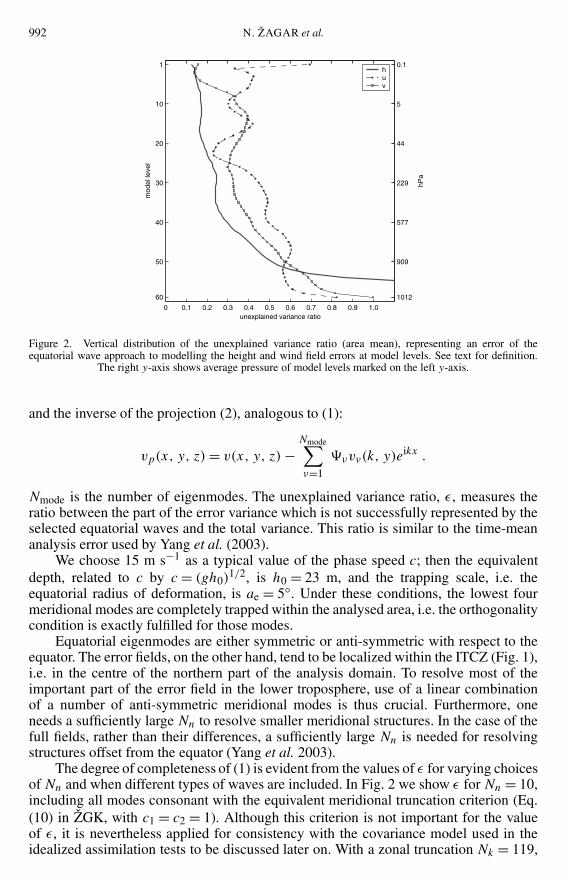
Figure 2. Vertical distribution of the unexplained variance ratio (area mean), representing an error of theequatorial wave approach to modelling the height and wind field errors at model levels. See text for definition.

The right y-axis shows average pressure of model levels marked on the left y-axis.

and the inverse of the projection (2), analogous to (1):

vp(x, y, z) = v(x, y, z) −Nmode∑ν=1

�νvν(k, y)eikx .

Nmode is the number of eigenmodes. The unexplained variance ratio, ε, measures theratio between the part of the error variance which is not successfully represented by theselected equatorial waves and the total variance. This ratio is similar to the time-meananalysis error used by Yang et al. (2003).

We choose 15 m s−1 as a typical value of the phase speed c; then the equivalentdepth, related to c by c = (gh0)

1/2, is h0 = 23 m, and the trapping scale, i.e. theequatorial radius of deformation, is ae = 5◦. Under these conditions, the lowest fourmeridional modes are completely trapped within the analysed area, i.e. the orthogonalitycondition is exactly fulfilled for those modes.

Equatorial eigenmodes are either symmetric or anti-symmetric with respect to theequator. The error fields, on the other hand, tend to be localized within the ITCZ (Fig. 1),i.e. in the centre of the northern part of the analysis domain. To resolve most of theimportant part of the error field in the lower troposphere, use of a linear combinationof a number of anti-symmetric meridional modes is thus crucial. Furthermore, oneneeds a sufficiently large Nn to resolve smaller meridional structures. In the case of thefull fields, rather than their differences, a sufficiently large Nn is needed for resolvingstructures offset from the equator (Yang et al. 2003).

The degree of completeness of (1) is evident from the values of ε for varying choicesof Nn and when different types of waves are included. In Fig. 2 we show ε for Nn = 10,including all modes consonant with the equivalent meridional truncation criterion (Eq.(10) in ZGK, with c1 = c2 = 1). Although this criterion is not important for the valueof ε, it is nevertheless applied for consistency with the covariance model used in theidealized assimilation tests to be discussed later on. With a zonal truncation Nk = 119,


a total of Nmode = 2937 eigenmodes are included in the expansion. The values shown inthe diagram are area means at each model level.

It can be seen that above the 500 hPa level (level 39), equatorial eigenmodessuccessfully represent 75–80% of the height- and 50–75% of the wind-field variances.The methodology is most successful at the levels where the errors, as measured byforecast differences, are largest. Below 500 hPa the amount of unexplained varianceincreases and becomes as large as 60% near 900 hPa (level 50). The unexplainedvariance is generally largest for the zonal wind component, except near the tropopauseand below 900 hPa. At these lowest levels, the methodology fails for all fields, especiallythat representing the height. Consequently, we shall not consider these levels in thesubsequent discussion.

A closer inspection of the spatial patterns of unexplained errors (the vp, up andhp fields) reveals that most of the tropospheric unexplained variance is located in theITCZ (not shown). This is the region where the assumed forecast errors do not displaythe expected symmetry with respect to the equator. Obviously, the number of anti-symmetric modes included in (1) do not suffice to reproduce the error pattern in theITCZ. We did not, however, try to further increase the value of Nn because of therequirement that eigenmodes remain equatorially trapped.

Figure 2 would assume a different character for other choices of eigenmodes. Forexample, in the case of Nn = 3 the unexplained variance ratio is much larger since threemeridional nodes only poorly resolve the structure of the error fields within the ITCZ.The zonal truncation, on the other hand, is of little importance since most of the spectralvariance is found below zonal wave number 20. An important part of the explainedvariance is due to EIG modes; including these has a major effect on the percentage ofthe explained wind-field variance, an effect larger than can be achieved by increasingNn. For example, in the case of Nn = 10, but without the EIG waves included in (1),the explained variance ratio for wind components is less than 40% in the troposphere,and above the tropopause it sharply decreases, invalidating the approach. On the otherhand, the representation of height errors is only slightly affected by a change of Nn,and almost wholly impervious to the choice of modes. This is due to the geopotentialgradients in the tropical atmosphere being weak and much more symmetric with respectto the equator than the wind field. Changes in c (as derived from the observed range ofh0) are unimportant for ε as compared to the two factors discussed above.

Of the three fields, the height field is best represented by the covariance model,except close to the surface, while the wind-field representation is most successful in theupper troposphere and near the tropopause. Except for the lowest ten model levels, themean values of ε range between 0.3 and 0.4, implying that in what follows we will beconcerned with the statistical structure of about 60−70% of the tropical variance.

(d) Meridional variation of errorsA spectral representation of errors retains full information about the scale variations

of the covariances but, as a consequence of the homogeneity assumption, provides no in-formation regarding their spatial variations. In the present case the homogeneity assump-tion is applied only in the zonal direction, which thus retains the meridional structurein the statistics. The implied error variances in grid-point space can be investigated byapplying a randomization method (Fisher 1996) to the spectral mode-based covariancemodel, followed by a transformation to grid-point space. This approach is based on thefact that the usual 3D-Var formulation in terms of normalized non-dimensional variables(e.g. �ν/γν) has a background-error covariance matrix equal to the identity matrix.Thus, one can take an ensemble of random vectors for �ν/γν , drawn from a Gaussian

994 N. ZAGAR et al.

0.5 1 1.5 2 2.5

20 S

15 S

10 S

5 S

EQ

5 N

10 N

15 N

20 N

(m/s), (m)

a

hmodel

htrue

umodel

utrue

vmodel

vtrue

0.5 1 1.5 2 2.5 3 3.5 4

20 S

15 S

10 S

5 S

EQ

5 N

10 N

15 N

20 N

(m/s), (m)

b

hmodel

htrue

umodel

utrue

vmodel

vtrue

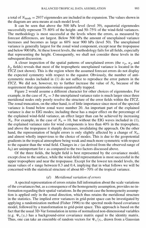
Figure 3. Meridional profiles of 12-hour forecast errors in the zonal wind (thin black lines) and the meridionalwind fields (thick grey lines) and the geopotential height (line with ◦ symbols). Dashed lines apply to the ‘truth’whereas full lines apply to the model (see text for further details). (a) Model level 43 (approximately 654 hPa),

(b) model level 27 (approximately 133 hPa).

distribution of zero mean and variance one, and obtain randomization estimates of theerror variances first in spectral space, and after further transformation, also in grid-pointspace. An application of this methodology is provided by Andersson et al. (2000).

The resulting randomization variances yield meridional profiles which can be com-pared with the zonally averaged profiles of the original error fields (generated by thedata-assimilation ensemble). The result, presented in Fig. 3 for two model levels, high-lights the main shortcomings of our methodology. In the lower troposphere (Fig. 3(a)),the error profiles of the ECMWF model have maxima at 8◦N, as illustrated in Fig. 1(a);in addition, errors increase south of 15◦S, especially those of the geopotential height. Incontrast, the error profiles modelled by equatorial waves display maxima at the equator,in particular for the wind. Error minima are located close to the meridional boundaries.The covariance model yields the best results in the upper troposphere (Fig. 3(b)), wherethe ECMWF forecast errors are not concentrated along the ITCZ (Fig. 1(b)). In thestratosphere our model retains the error maxima at the equator (not shown) while the‘true’ errors of all the fields to a large extent become homogeneous. Equatorially-centrederror profiles are caused by Kelvin-wave correlations, to be illustrated in section 4.

Another shortcoming noticeable in Fig. 3 arises from the wind and mass fieldsbeing analysed together. Their error coupling is responsible for the insufficiently largeamplitudes of the modelled height errors in the troposphere. This interaction also yieldsunrealistically large amplitudes of the wind-field errors in the stratosphere, where theECMWF geopotential errors increase.

The spectral mode-based covariance model thus captures a significant part of theerror variance that is symmetric around the equator, but far less of the asymmetric part.Note, however, that in a practical implementation of the derived covariance model in avariational data-assimilation scheme, the unexplained part of the tropical error variancewould be analysed in a univariate fashion.


0 5 10 15 20 25 30 35 40 45 50 5560

50

40

30

20

10

1

leve

l

%

EREEIGWEIGKEMRGWMRG

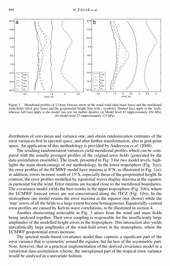
Figure 4. Vertical distribution of the variance among various equatorial eigenmodes: equatorial Rossby (ER)modes, eastward-propagating (EEIG) and westward-propagating (WEIG) equatorial inertio-gravity modes, Kelvin(K) modes, eastward- (EMRG) and westward-propagating (WMRG) mixed Rossby–gravity waves. The x-axis

notation applies to the percentage of the total explained variance.

3. VARIANCES AND VERTICAL CORRELATIONS

(a) VariancesIn Fig. 4 we illustrate the tropical covariance model in terms of its variance

distribution between the different types of equatorial waves. Among individual modes,the largest part of the variance pertains to Rossby-type motion. Its profile displays asharp decrease of the variance in the vicinity of the tropopause, with a broad minimumin the range from 5 to 50 hPa (levels 11 to 22). Such a profile shape is in agreement withstrong easterlies in the stratosphere during the study period of October 2000; in thesecircumstances westward-propagating waves do not satisfy the criterion for vertical wavepropagation (Charney and Drazin 1961). Within the troposphere, the variance assignedto ER waves is between 40% and 50%, and is largest at levels between 150 and 300 hPa(levels 28 and 34, respectively). Contributions from various meridional modes decreaseas n increases. The variance profile for the lowest two modes adheres to the shape of thetotal profile. For higher modes, stratospheric variance is small. Modes five and higherthus make no contribution to the variance in the stratosphere, whereas they contribute afew percent of the variance in the troposphere (not shown).

Profiles of ER and EIG modes have the opposite variance phase in the troposphere,while EEIG and WEIG modes are 180◦ out of phase in the stratosphere. Otherwise, thepercentage of variance contributed by EEIG and WEIG modes, respectively, is similar inthe troposphere, except at levels 26–34 corresponding to the range 100–300 hPa, whereWEIG modes play a more important role. In the stratosphere, EEIG waves have anabsolute maximum of variance around the 6 hPa level (model level 12). Together, EEIGand WEIG modes constitute 40–50% of the variance in the troposphere. In contrast toER waves, EIG modes demonstrate the same vertical profile of variance for all n (notshown).

996 N. ZAGAR et al.

1 2 3 4 6 10 20 40 70 11010

4

103

102

101

100

101

102

zonal wave number

2

a

level 15level 39level 48

1 2 3 4 6 10 20 40 70 11010

4

103

102

101

100

101

102

zonal wave number

2

b


1 2 3 4 6 10 20 40 70 11010

4

103

102

101

100

101

102

zonal wave number

2

c


1 2 3 4 6 10 20 40 70 11010

4

103

102

101

100

101

102

zonal wave number

2

d


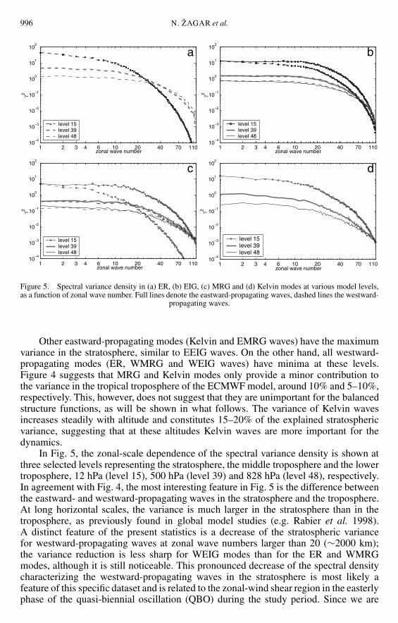
Figure 5. Spectral variance density in (a) ER, (b) EIG, (c) MRG and (d) Kelvin modes at various model levels,as a function of zonal wave number. Full lines denote the eastward-propagating waves, dashed lines the westward-

propagating waves.

Other eastward-propagating modes (Kelvin and EMRG waves) have the maximumvariance in the stratosphere, similar to EEIG waves. On the other hand, all westward-propagating modes (ER, WMRG and WEIG waves) have minima at these levels.Figure 4 suggests that MRG and Kelvin modes only provide a minor contribution tothe variance in the tropical troposphere of the ECMWF model, around 10% and 5–10%,respectively. This, however, does not suggest that they are unimportant for the balancedstructure functions, as will be shown in what follows. The variance of Kelvin wavesincreases steadily with altitude and constitutes 15–20% of the explained stratosphericvariance, suggesting that at these altitudes Kelvin waves are more important for thedynamics.

In Fig. 5, the zonal-scale dependence of the spectral variance density is shown atthree selected levels representing the stratosphere, the middle troposphere and the lowertroposphere, 12 hPa (level 15), 500 hPa (level 39) and 828 hPa (level 48), respectively.In agreement with Fig. 4, the most interesting feature in Fig. 5 is the difference betweenthe eastward- and westward-propagating waves in the stratosphere and the troposphere.At long horizontal scales, the variance is much larger in the stratosphere than in thetroposphere, as previously found in global model studies (e.g. Rabier et al. 1998).A distinct feature of the present statistics is a decrease of the stratospheric variancefor westward-propagating waves at zonal wave numbers larger than 20 (∼2000 km);the variance reduction is less sharp for WEIG modes than for the ER and WMRGmodes, although it is still noticeable. This pronounced decrease of the spectral densitycharacterizing the westward-propagating waves in the stratosphere is most likely afeature of this specific dataset and is related to the zonal-wind shear region in the easterlyphase of the quasi-biennial oscillation (QBO) during the study period. Since we are


using a sample representative of only one phase of the QBO, the present results may notbe representative of the long-term statistics for the tropics. It is likely that the statisticsfor the dataset from the opposite phase of the QBO would look different, suggestingthat significant temporal variations could be present in longer-term time series of suchstatistics. A more thorough investigation of this issue is, however, beyond the scope ofthis study.

Among the six different wave types, ER modes dominate the spectra at all scalesexcept in the stratosphere. Here, all eastward-propagating modes have a larger variancethan the ER waves for k > 10, with Kelvin waves becoming relatively more importantat long scales; the latter feature is in agreement with observational and theoreticalstudies of the role of Kelvin waves in the equatorial stratosphere. The greatest part ofthe spectral variance in the stratosphere is, however, associated with EIG waves. Theirdominance over the Kelvin and MRG modes is in agreement with recent observationaland modelling studies (e.g. Dunkerton 1997; Giorgetta et al. 2002), suggesting that thegravity waves carry approximately half of the momentum flux required to drive theQBO.

Based on a comparison between 3-, 12- and 24-hour forecasts (figure not shown),the partitioning of variance between modes and scales does not change much withforecast time. The main difference between the 3- and 24-hour forecasts is an increaseof the Kelvin- and ER-wave variance in the stratosphere (2–3% and ∼5%, respectively),at the expense of the EIG-wave variance. This quantity reduces by a few percent alsoin the troposphere, with a corresponding increase of the ER-wave variance. MRG-wavevariance remains virtually unchanged. Based on a comparison between the results forthe standard case of h0 = 23 m and those obtained when h0 is taken equal to 50 and250 m, the sensitivity with respect to c is not significant.

It might be argued that a significant fraction of the variance associated with EIGmodes could arise from model deficiencies, especially in the early stages of the forecast.Possibly the model has systematic errors, but those are ignored in strong-constraint 4D-Var. The background-error term should describe the de facto statistics of backgrounderrors. If these contain more EIG-wave motion than deemed desirable, such modeldeficiencies could be addressed through a model-error term (i.e. weak-constraint 4D-Var). In this paper, we only attempt to diagnose the equatorial background errors in thecurrent ECMWF analysis, and do not attempt to formulate a background-error term foruse in an analysis system. This latter task would first require dealing with the 30–40%of the variance not described by the projection onto equatorial modes.

(b) Vertical correlationsVertical correlations are calculated for all model levels, but we disregard levels 50–

60 (900–1012 hPa) due to the small percentage of variance here which can be explainedusing the equatorial wave approach. The shape of correlation depends on the wave typeas well as the altitude (Figs. 6–8). Moving upwards and towards smaller scales generallygives rise to more narrow correlations. The narrowing of vertical correlations for smallerscales is seen mainly for the ER and Kelvin modes, to a lesser extent for the MRG modesand almost not at all for the EIG waves.

The broadening at large scales of the ER-wave correlations (Fig. 6) begins ap-proximately at zonal wave number 20, and is larger at n = 1 (Fig. 6(a)) than for thehigher modes (Fig. 6(b)). However, comparing ER correlations for the same n it may benoted that the narrowing of the correlations with altitude primarily applies to the model-level space. If the vertical coordinate is height, the shapes of the correlations for smallzonal wave numbers would be more-or-less similar at various altitudes. Such narrowing

998 N. ZAGAR et al.

1 2 3 4 6 10 20 40 70 10060

50

40

30

20

10

1

leve

l

k

0.20.2

0.2

0.2

0.2

0.40.40.4

0.6 0.60.6

0.8 0.80.81 11 1 11 11 111

a

1 2 3 4 6 10 20 40 70 10060

50

40

30

20

10

1

leve

l

k

0.2 0.2

0.2

0.2

0.4 0.4

0.40.6

0.60.6

0.8 0.80.8 11 11 1 11 11

0.2 0.2

b

1 2 3 4 6 10 20 40 70 10060

50

40

30

20

10

1

leve

l

k

0.20.2

0.2

0.2

0.2

0.2

0.20.20.2 0.

20.2 0.2

0.20.2

0.2

0.4 0.4

0.40.40.4

0.6

0.60.6

0.8 0.8

0.81 11 1 111 111 111

c

1 2 3 4 6 10 20 40 70 10060

50

40

30

20

10

1

leve

l

k

0.2

0.20.2

0.2

0.4 0.40.4

0.60.60.6

0.8 0.80.81 1 1 11 1 11 1

0.4

0.2

0.2

0.2 0.20.2

d

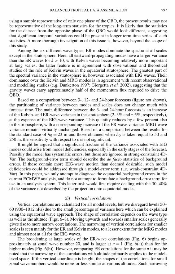
Figure 6. Vertical correlations for ER modes, as a function of zonal wave number k. (a) n = 1 and (b) n = 2 atmodel level 27 (approximately 133 hPa); (c) n = 1 at model level 43 (approximately 654 hPa); (d) n = 1 at model

level 15 (approximately 12 hPa). Isolines every 0.2 with zero isoline omitted.

in model space could indicate an insufficient vertical resolution. Thus, Lindzen andFox-Rabinovitz (1989) demonstrated that the consistency requirement for the horizontaland vertical resolution demands a higher vertical resolution in the tropics than at mid-latitudes.

Vertical correlations in the troposphere are not symmetric; throughout this re-gion correlations with levels below are much stronger than those with levels above(Figs. 6(a)–(c)). The underlying physical mechanism is, most likely, convection. Thishypothesis is given added weight by the fact that the stratospheric correlations do notdisplay such an asymmetry.

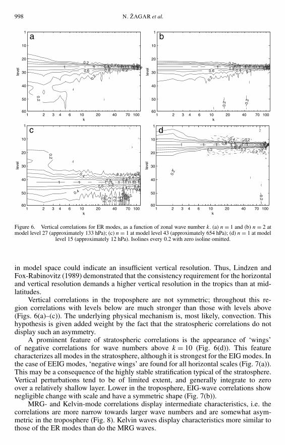
A prominent feature of stratospheric correlations is the appearance of ‘wings’of negative correlations for wave numbers above k = 10 (Fig. 6(d)). This featurecharacterizes all modes in the stratosphere, although it is strongest for the EIG modes. Inthe case of EEIG modes, ‘negative wings’ are found for all horizontal scales (Fig. 7(a)).This may be a consequence of the highly stable stratification typical of the stratosphere.Vertical perturbations tend to be of limited extent, and generally integrate to zeroover a relatively shallow layer. Lower in the troposphere, EIG-wave correlations shownegligible change with scale and have a symmetric shape (Fig. 7(b)).

MRG- and Kelvin-mode correlations display intermediate characteristics, i.e. thecorrelations are more narrow towards larger wave numbers and are somewhat asym-metric in the troposphere (Fig. 8). Kelvin waves display characteristics more similar tothose of the ER modes than do the MRG waves.


1 2 3 4 6 10 20 40 70 10060

50

40

30

20

10

1

leve

l

k

0.2

0.2

0.2

0.20.20.2

0.20.2

0.4 0.40.4

0.60.60.6

0.8 0.80.81 1 11 11 11 1 11 111

0.60.4

0.4

0.40.2

0.2

0.2 0.2

a

1 2 3 4 6 10 20 40 70 10060

50

40

30

20

10

1

leve

l

k

0.2

0.2

0.20.20.2

0.2

0.4 0.4

0.40.4

0.6 0.6

0.6

0.8 0.80.8

1 11 11 11 111 1

0.20.2

0.2

b

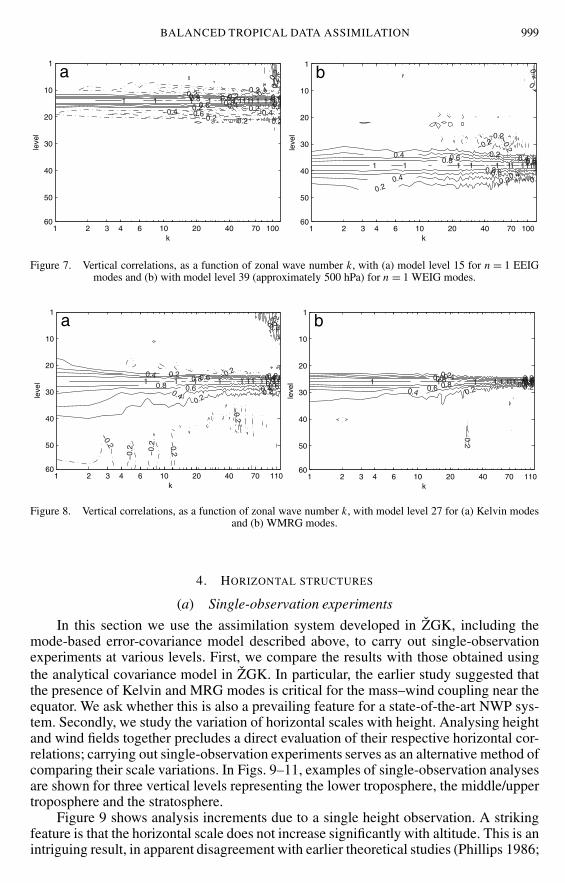
Figure 7. Vertical correlations, as a function of zonal wave number k, with (a) model level 15 for n = 1 EEIGmodes and (b) with model level 39 (approximately 500 hPa) for n = 1 WEIG modes.

1 2 3 4 6 10 20 40 70 11060

50

40

30

20

10

1

leve

l

k

0.2

0.2

0.2 0.2

0.20.2

0.2

0.4 0.4

0.40.4

0.6 0.60.6 0.6

0.8 0.80.8 0.811 1 11 11 111 11

0.2

0.2 0.2 0.2

0.2

0.2a

1 2 3 4 6 10 20 40 70 11060

50

40

30

20

10

1

leve

l

k

0.2 0.2

0.2 0.20.4 0.4

0.40.4

0.6 0.60.6 0.6

0.8 0.80.8 0.81 11 1111 111 11

0.2

b

Figure 8. Vertical correlations, as a function of zonal wave number k, with model level 27 for (a) Kelvin modesand (b) WMRG modes.

4. HORIZONTAL STRUCTURES

(a) Single-observation experiments

In this section we use the assimilation system developed in ZGK, including themode-based error-covariance model described above, to carry out single-observationexperiments at various levels. First, we compare the results with those obtained usingthe analytical covariance model in ZGK. In particular, the earlier study suggested thatthe presence of Kelvin and MRG modes is critical for the mass–wind coupling near theequator. We ask whether this is also a prevailing feature for a state-of-the-art NWP sys-tem. Secondly, we study the variation of horizontal scales with height. Analysing heightand wind fields together precludes a direct evaluation of their respective horizontal cor-relations; carrying out single-observation experiments serves as an alternative method ofcomparing their scale variations. In Figs. 9–11, examples of single-observation analysesare shown for three vertical levels representing the lower troposphere, the middle/uppertroposphere and the stratosphere.

Figure 9 shows analysis increments due to a single height observation. A strikingfeature is that the horizontal scale does not increase significantly with altitude. This is anintriguing result, in apparent disagreement with earlier theoretical studies (Phillips 1986;

1000 N. ZAGAR et al.

80 W 60 W 40 W

15 S

10 S

5 S

EQ

5 N

10 N

15 Na

1 m/s

80 W 60 W 40 W

15 S

10 S

5 S

EQ

5 N

10 N

15 Nb

80 W 60 W 40 W

15 S

10 S

5 S

EQ

5 N

10 N

15 Nc

80 W 60 W 40 W10 S

5 S

EQ

5 N

10 N

15 N

d

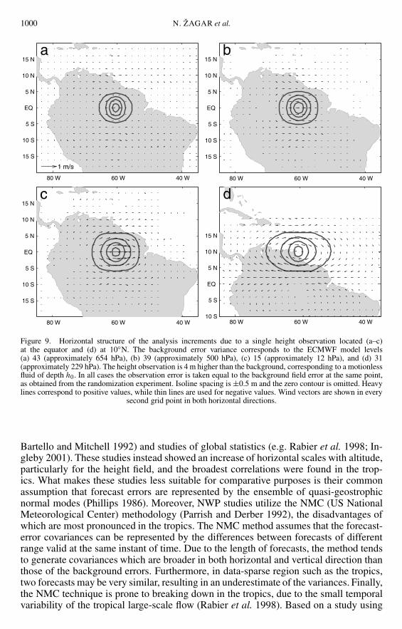
Figure 9. Horizontal structure of the analysis increments due to a single height observation located (a–c)at the equator and (d) at 10◦N. The background error variance corresponds to the ECMWF model levels(a) 43 (approximately 654 hPa), (b) 39 (approximately 500 hPa), (c) 15 (approximately 12 hPa), and (d) 31(approximately 229 hPa). The height observation is 4 m higher than the background, corresponding to a motionlessfluid of depth h0. In all cases the observation error is taken equal to the background field error at the same point,as obtained from the randomization experiment. Isoline spacing is ±0.5 m and the zero contour is omitted. Heavylines correspond to positive values, while thin lines are used for negative values. Wind vectors are shown in every

second grid point in both horizontal directions.

Bartello and Mitchell 1992) and studies of global statistics (e.g. Rabier et al. 1998; In-gleby 2001). These studies instead showed an increase of horizontal scales with altitude,particularly for the height field, and the broadest correlations were found in the trop-ics. What makes these studies less suitable for comparative purposes is their commonassumption that forecast errors are represented by the ensemble of quasi-geostrophicnormal modes (Phillips 1986). Moreover, NWP studies utilize the NMC (US NationalMeteorological Center) methodology (Parrish and Derber 1992), the disadvantages ofwhich are most pronounced in the tropics. The NMC method assumes that the forecast-error covariances can be represented by the differences between forecasts of differentrange valid at the same instant of time. Due to the length of forecasts, the method tendsto generate covariances which are broader in both horizontal and vertical direction thanthose of the background errors. Furthermore, in data-sparse region such as the tropics,two forecasts may be very similar, resulting in an underestimate of the variances. Finally,the NMC technique is prone to breaking down in the tropics, due to the small temporalvariability of the tropical large-scale flow (Rabier et al. 1998). Based on a study using


80 W 60 W 40 W

15 S

10 S

5 S

EQ

5 N

10 N

15 Na

4 m/s

80 W 60 W 40 W

15 S

10 S

5 S

EQ

5 N

10 N

15 Nb

80 W 60 W 40 W

15 S

10 S

5 S

EQ

5 N

10 N

15 Nc

80 W 60 W 40 W10 S

5 S

EQ

5 N

10 N

15 N

d

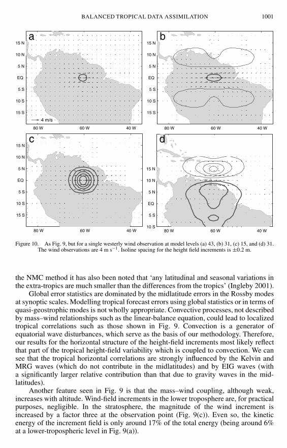
Figure 10. As Fig. 9, but for a single westerly wind observation at model levels (a) 43, (b) 31, (c) 15, and (d) 31.The wind observations are 4 m s−1. Isoline spacing for the height field increments is ±0.2 m.

the NMC method it has also been noted that ‘any latitudinal and seasonal variations inthe extra-tropics are much smaller than the differences from the tropics’ (Ingleby 2001).

Global error statistics are dominated by the midlatitude errors in the Rossby modesat synoptic scales. Modelling tropical forecast errors using global statistics or in terms ofquasi-geostrophic modes is not wholly appropriate. Convective processes, not describedby mass–wind relationships such as the linear-balance equation, could lead to localizedtropical correlations such as those shown in Fig. 9. Convection is a generator ofequatorial wave disturbances, which serve as the basis of our methodology. Therefore,our results for the horizontal structure of the height-field increments most likely reflectthat part of the tropical height-field variability which is coupled to convection. We cansee that the tropical horizontal correlations are strongly influenced by the Kelvin andMRG waves (which do not contribute in the midlatitudes) and by EIG waves (witha significantly larger relative contribution than that due to gravity waves in the mid-latitudes).

Another feature seen in Fig. 9 is that the mass–wind coupling, although weak,increases with altitude. Wind-field increments in the lower troposphere are, for practicalpurposes, negligible. In the stratosphere, the magnitude of the wind increment isincreased by a factor three at the observation point (Fig. 9(c)). Even so, the kineticenergy of the increment field is only around 17% of the total energy (being around 6%at a lower-tropospheric level in Fig. 9(a)).


80 W 60 W 40 W

15 S

10 S

5 S

EQ

5 N

10 N

15 Na

4 m/s

80 W 60 W 40 W

15 S

10 S

5 S

EQ

5 N

10 N

15 Nb

80 W 60 W 40 W

15 S

10 S

5 S

EQ

5 N

10 N

15 Nc

80 W 60 W 40 W10 S

5 S

EQ

5 N

10 N

15 N

d

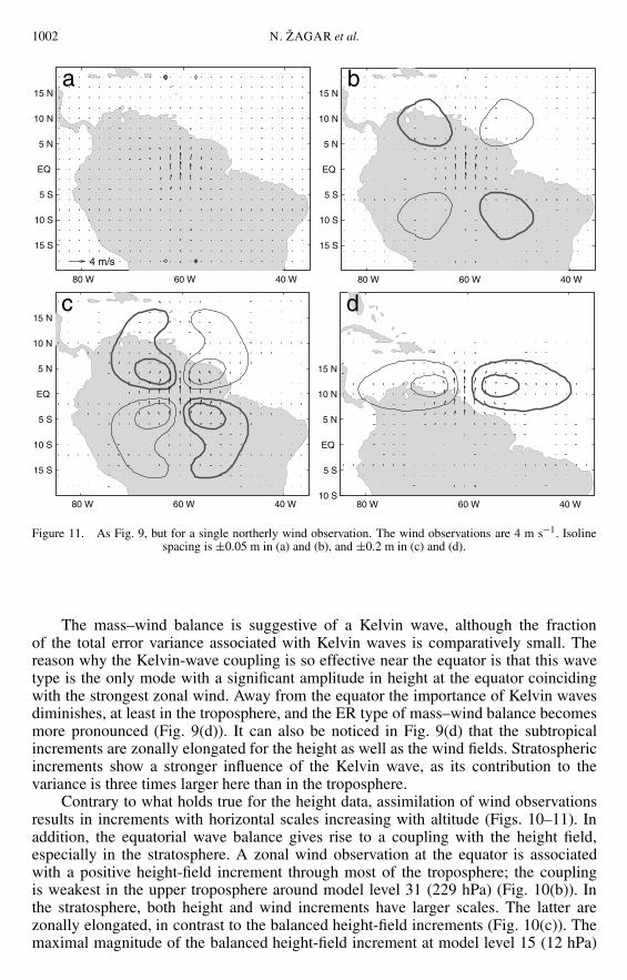
Figure 11. As Fig. 9, but for a single northerly wind observation. The wind observations are 4 m s−1. Isolinespacing is ±0.05 m in (a) and (b), and ±0.2 m in (c) and (d).

The mass–wind balance is suggestive of a Kelvin wave, although the fractionof the total error variance associated with Kelvin waves is comparatively small. Thereason why the Kelvin-wave coupling is so effective near the equator is that this wavetype is the only mode with a significant amplitude in height at the equator coincidingwith the strongest zonal wind. Away from the equator the importance of Kelvin wavesdiminishes, at least in the troposphere, and the ER type of mass–wind balance becomesmore pronounced (Fig. 9(d)). It can also be noticed in Fig. 9(d) that the subtropicalincrements are zonally elongated for the height as well as the wind fields. Stratosphericincrements show a stronger influence of the Kelvin wave, as its contribution to thevariance is three times larger here than in the troposphere.

Contrary to what holds true for the height data, assimilation of wind observationsresults in increments with horizontal scales increasing with altitude (Figs. 10–11). Inaddition, the equatorial wave balance gives rise to a coupling with the height field,especially in the stratosphere. A zonal wind observation at the equator is associatedwith a positive height-field increment through most of the troposphere; the couplingis weakest in the upper troposphere around model level 31 (229 hPa) (Fig. 10(b)). Inthe stratosphere, both height and wind increments have larger scales. The latter arezonally elongated, in contrast to the balanced height-field increments (Fig. 10(c)). Themaximal magnitude of the balanced height-field increment at model level 15 (12 hPa)


is approximately 3.6 times larger than at model level 43 (654 hPa); the correspondingpotential-energy contribution is increased from 2% at level 43 to 7% at level 15. Thebalance at the equator is dominated by Kelvin waves, but at a distance from the equator,height-field increments become geostrophic and zonally elongated (Fig. 10(d)), in fullagreement with quasi-geostrophic theory. By comparing Fig. 10(d) with Fig. 10(b) itcan also be seen that equator-centred modes considerably reduce the magnitude of thebalanced height field.

The increase of the amplitude of the balanced height increments with altitudeis largest for a meridional wind observation (Fig. 11). When this is centred on theequator (Figs. 11(a)–(c)), the shape of the increments resembles an MRG wave. Withthe observation located at 10◦N, the increments appear nearly geostrophic (Fig. 11(d))and very similar to those found in the midlatitude case (e.g. Courtier et al. 1998), exceptfor a broader zonal scale. A significant enlargement of the horizontal scale of a height-field increment with altitude is visible (note that the isoline spacing in Figs. 11(c)–(d) isfour times larger than in Figs. 11(a)–(b)). The potential-energy content increases fromzero at level 43 (654 hPa) to around 3% of the total energy at level 15 (12 hPa).

(b) Sensitivity experiments

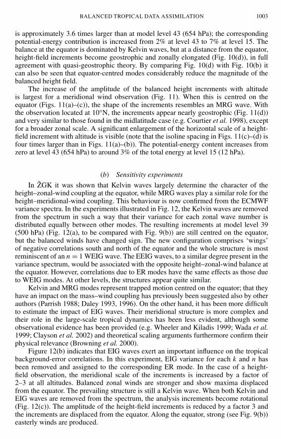
In ZGK it was shown that Kelvin waves largely determine the character of theheight–zonal-wind coupling at the equator, while MRG waves play a similar role for theheight–meridional-wind coupling. This behaviour is now confirmed from the ECMWFvariance spectra. In the experiments illustrated in Fig. 12, the Kelvin waves are removedfrom the spectrum in such a way that their variance for each zonal wave number isdistributed equally between other modes. The resulting increments at model level 39(500 hPa) (Fig. 12(a), to be compared with Fig. 9(b)) are still centred on the equator,but the balanced winds have changed sign. The new configuration comprises ‘wings’of negative correlations south and north of the equator and the whole structure is mostreminiscent of an n = 1 WEIG wave. The EEIG waves, to a similar degree present in thevariance spectrum, would be associated with the opposite height–zonal-wind balance atthe equator. However, correlations due to ER modes have the same effects as those dueto WEIG modes. At other levels, the structures appear quite similar.

Kelvin and MRG modes represent trapped motion centred on the equator; that theyhave an impact on the mass–wind coupling has previously been suggested also by otherauthors (Parrish 1988; Daley 1993, 1996). On the other hand, it has been more difficultto estimate the impact of EIG waves. Their meridional structure is more complex andtheir role in the large-scale tropical dynamics has been less evident, although someobservational evidence has been provided (e.g. Wheeler and Kiladis 1999; Wada et al.1999; Clayson et al. 2002) and theoretical scaling arguments furthermore confirm theirphysical relevance (Browning et al. 2000).

Figure 12(b) indicates that EIG waves exert an important influence on the tropicalbackground-error correlations. In this experiment, EIG variance for each k and n hasbeen removed and assigned to the corresponding ER mode. In the case of a height-field observation, the meridional scale of the increments is increased by a factor of2–3 at all altitudes. Balanced zonal winds are stronger and show maxima displacedfrom the equator. The prevailing structure is still a Kelvin wave. When both Kelvin andEIG waves are removed from the spectrum, the analysis increments become rotational(Fig. 12(c)). The amplitude of the height-field increments is reduced by a factor 3 andthe increments are displaced from the equator. Along the equator, strong (see Fig. 9(b))easterly winds are produced.


80 W 60 W 40 W

15 S

10 S

5 S

EQ

5 N

10 N

15 Na

1 m/s

80 W 60 W 40 W

15 S

10 S

5 S

EQ

5 N

10 N

15 N

1 m/s

b

80 W 60 W 40 W

15 S

10 S

5 S

EQ

5 N

10 N

15 Nc

1 m/s

80 W 60 W 40 W

15 S

10 S

5 S

EQ

5 N

10 N

15 N

4 m/s

d

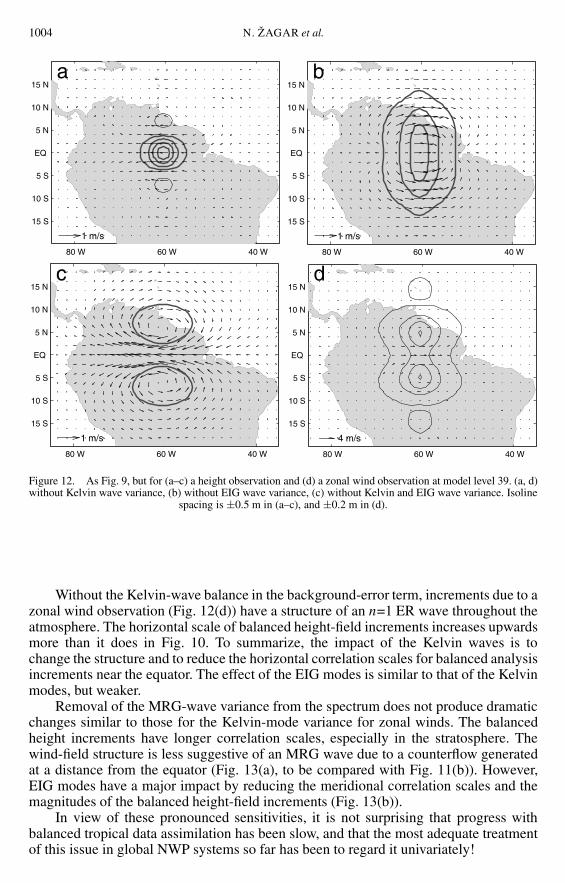
Figure 12. As Fig. 9, but for (a–c) a height observation and (d) a zonal wind observation at model level 39. (a, d)without Kelvin wave variance, (b) without EIG wave variance, (c) without Kelvin and EIG wave variance. Isoline

spacing is ±0.5 m in (a–c), and ±0.2 m in (d).

Without the Kelvin-wave balance in the background-error term, increments due to azonal wind observation (Fig. 12(d)) have a structure of an n=1 ER wave throughout theatmosphere. The horizontal scale of balanced height-field increments increases upwardsmore than it does in Fig. 10. To summarize, the impact of the Kelvin waves is tochange the structure and to reduce the horizontal correlation scales for balanced analysisincrements near the equator. The effect of the EIG modes is similar to that of the Kelvinmodes, but weaker.

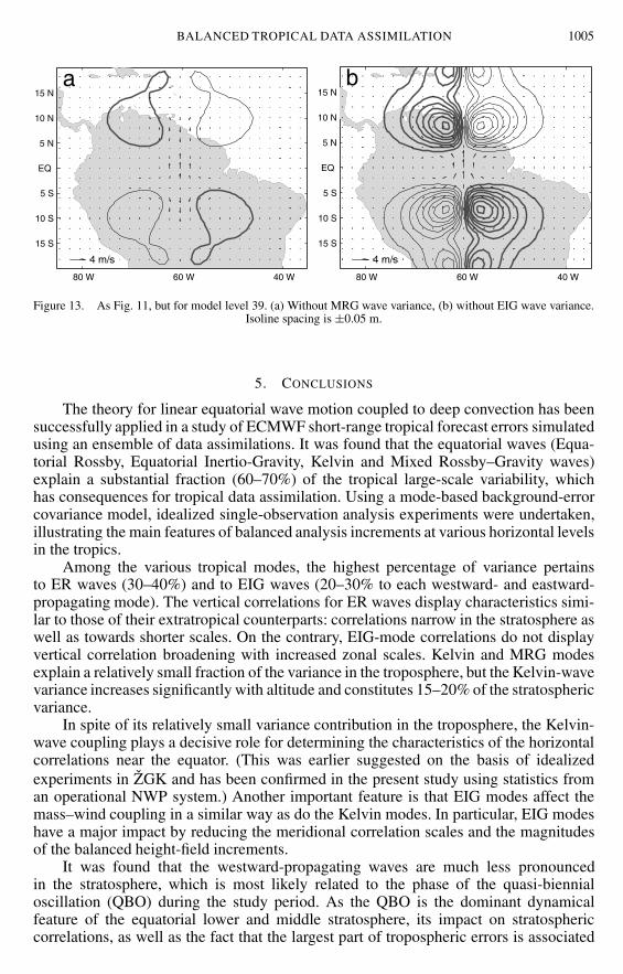
Removal of the MRG-wave variance from the spectrum does not produce dramaticchanges similar to those for the Kelvin-mode variance for zonal winds. The balancedheight increments have longer correlation scales, especially in the stratosphere. Thewind-field structure is less suggestive of an MRG wave due to a counterflow generatedat a distance from the equator (Fig. 13(a), to be compared with Fig. 11(b)). However,EIG modes have a major impact by reducing the meridional correlation scales and themagnitudes of the balanced height-field increments (Fig. 13(b)).

In view of these pronounced sensitivities, it is not surprising that progress withbalanced tropical data assimilation has been slow, and that the most adequate treatmentof this issue in global NWP systems so far has been to regard it univariately!


80 W 60 W 40 W

15 S

10 S

5 S

EQ

5 N

10 N

15 Na

4 m/s

80 W 60 W 40 W

15 S

10 S

5 S

EQ

5 N

10 N

15 Nb

4 m/s

Figure 13. As Fig. 11, but for model level 39. (a) Without MRG wave variance, (b) without EIG wave variance.Isoline spacing is ±0.05 m.

5. CONCLUSIONS

The theory for linear equatorial wave motion coupled to deep convection has beensuccessfully applied in a study of ECMWF short-range tropical forecast errors simulatedusing an ensemble of data assimilations. It was found that the equatorial waves (Equa-torial Rossby, Equatorial Inertio-Gravity, Kelvin and Mixed Rossby–Gravity waves)explain a substantial fraction (60–70%) of the tropical large-scale variability, whichhas consequences for tropical data assimilation. Using a mode-based background-errorcovariance model, idealized single-observation analysis experiments were undertaken,illustrating the main features of balanced analysis increments at various horizontal levelsin the tropics.

Among the various tropical modes, the highest percentage of variance pertainsto ER waves (30–40%) and to EIG waves (20–30% to each westward- and eastward-propagating mode). The vertical correlations for ER waves display characteristics simi-lar to those of their extratropical counterparts: correlations narrow in the stratosphere aswell as towards shorter scales. On the contrary, EIG-mode correlations do not displayvertical correlation broadening with increased zonal scales. Kelvin and MRG modesexplain a relatively small fraction of the variance in the troposphere, but the Kelvin-wavevariance increases significantly with altitude and constitutes 15–20% of the stratosphericvariance.

In spite of its relatively small variance contribution in the troposphere, the Kelvin-wave coupling plays a decisive role for determining the characteristics of the horizontalcorrelations near the equator. (This was earlier suggested on the basis of idealizedexperiments in ZGK and has been confirmed in the present study using statistics froman operational NWP system.) Another important feature is that EIG modes affect themass–wind coupling in a similar way as do the Kelvin modes. In particular, EIG modeshave a major impact by reducing the meridional correlation scales and the magnitudesof the balanced height-field increments.

It was found that the westward-propagating waves are much less pronouncedin the stratosphere, which is most likely related to the phase of the quasi-biennialoscillation (QBO) during the study period. As the QBO is the dominant dynamicalfeature of the equatorial lower and middle stratosphere, its impact on stratosphericcorrelations, as well as the fact that the largest part of tropospheric errors is associated


with the intertropical convergence zone (ITCZ), suggest that the background-errorstatistics should vary with time. The high concentration of errors along the ITCZ, i.e.an asymmetric distribution with respect to the equator, has been found to be the mainimpediment for a methodology based on equatorial wave theory.

Application of quasi-geostrophic theory in the tropics results in zonally elongatedhorizontal structures, since according to this theory the horizontal scales vary in accor-dance with the Rossby deformation radius. However, quasi-geostrophic considerationsdo not take into account the possible influence exerted by non-rotational tropical modeson the horizontal correlations near the equator. The covariance model derived in thepresent study retains this influence, as illustrated by the single-observations assimila-tion results. In particular, it was found that the increase with altitude of the horizontal-correlation scale for height is less pronounced than that which would result from thequasi-geostrophic approach or from globally-averaged error statistics. It was also foundthat the correlations are vertically asymmetric. Both features are linked to deep tropicalconvection acting to generate equatorial wave motion.

The background-error covariance model in the ECMWF 4D-Var scheme is ef-fectively univariate near the equator, similar to many other global data-assimilationschemes. An appropriate projection of tropical analysis increments onto equatorialmodes is therefore not ensured. Excessive large-scale divergence in the increments maybe a contributing factor for the overestimated Hadley circulation observed in ECMWFoperational analysis and in the ECMWF 40-year re-analysis (ERA-40) (Uppala 2001).Too large analysed amounts of gravity waves in the lower stratosphere/upper tropo-sphere may also contribute to the overestimate of the Brewer–Dobson circulation alsoobserved in the operational analyses as well as in ERA-40. An approach that combinestropical and midlatitude dynamics and produces balanced increments globally is thusrequired for further progress.

To summarize, a diagnostic study of the tropical background errors in the currentECMWF analysis has revealed a number of distinct features compared to global errorstatistics. This work can be regarded as one of several steps towards improving thebackground-error term used in a global analysis system. Remaining tasks includedealing with the 30–40% of the variance not described by the method, analysis of thevertical eigenvectors, the study of longer-term variations and not least the mathematicalchallenges involved in formulating a global three-dimensional covariance model whichincludes these equatorially trapped modes.

ACKNOWLEDGEMENTS

The authors would like to thank Erland Kallen and Nils Gustafsson (MISU) foradvice and stimulating discussions during the course of this work, and to them, AdrianSimmons (ECMWF) and Peter Lundberg (MISU) for reading the paper and theirrelevant comments. We also thank Agathe Untch (ECMWF) for discussions of theresults, and her and Joan Alexander (CORA) for commenting on the role of the QBO.

APPENDIX

A data-assimilation ensemble method for generation of background error samplesLet us consider the analysis system as a ‘black box’, which delivers an analysis xa

given a background xb and a set of observations represented by the vector y:

xa = f(xb, y). (A.1)


Note that, with the exception of the background, y includes all the inputs to the analysissystem. In particular, it may include quantities such as sea surface temperature.

We will also consider the forecast for time T with initial conditions provided by theanalysis:

xf(T ) = MT (xa). (A.2)

The analysis, background and observation errors are

εa = xa − xt (A.3)

εb = xb − xt (A.4)

εo = y − yt (A.5)

where xt is the discretization of the true state, and where yt is the vector of true valuesof the observed quantities. The forecast error is

εf(T ) = xf(T ) − xt(T ), (A.6)

where xt(T ) is the true state at time T .We will denote by εs the error of an analysis made with perfect background and

observations, and by εm(T ) the error of a forecast made with perfect initial conditions:

εs = f(xt, yt) − xt (A.7)

εm(T ) = MT (xt) − xt(T ). (A.8)

Assuming that f is differentiable at (xt, yt), the analysis error is given by a Taylorexpansion of f about (xt, yt):

εa = ∂f(xt, yt)

∂xbεb + ∂f(xt, yt)

∂yεo + εs + O(ε2), (A.9)

where ∂f/∂xb and ∂f/∂y denote the Jacobian matrices of partial derivatives of f withrespect to the elements of xb and y. Similarly, if MT is differentiable at xt, then theforecast error is

εf(T ) = ∂MT (xt)

∂xεa + εm(T ) + O(ε2). (A.10)

Now consider an analysis made by adding perturbations ζ and η to xb and y, withthe result further perturbed by the addition of ω:

xa = f(xb + ζ, y + η) + ω. (A.11)

The error in xa can be expressed as a Taylor expansion about (xt, yt):

εa = ∂f(xt, yt)

∂xb(εb + ζ ) + ∂f(xt, yt)

∂y(εo + η) + (εs + ω) + O(ε2). (A.12)

If we now consider the difference δxa between two perturbed analyses, made withdifferent perturbations, we have:

δxa = ∂f(xt, yt)

∂xbδζ + ∂f(xt, yt)

∂yδη + δω + O(ε2), (A.13)

where δζ , δη and δω are the differences between the corresponding perturbations forthe two analyses.


Suppose now that the perturbations are chosen so that the covariance matrix forthe vector (δζ, δη, δω)T is twice the corresponding covariance matrix for (εb, εo, εs)T.This may be achieved by perturbing each analysis with different random errors drawnfrom the distribution of (εb, εo, εs)T. Comparing (A.9) and (A.13), we see that, to firstorder in ε, the covariance matrix for δxa is twice the covariance matrix for the analysiserror εa of the unperturbed analysis.

Next consider a forecast with initial condition xa, and with an additional perturba-tion, ξ :

xf = MT (xa) + ξ. (A.14)

The error of this forecast is:

εf(T ) = ∂MT (xt)

∂xεa + ξ + εm(T ) + O(ε2). (A.15)

By an argument similar to that given above, the difference between two forecastsmade from differently perturbed analyses is:

δxf(T ) = ∂MT (xt)

∂xδxa + δξ + O(ε2). (A.16)

Comparing (A.10) and (A.16), we see that if the vector (δxa, δξ)T has a covariancematrix equal to twice that of (εa, εm(T ))T, then to first order, δxf(T ) will have acovariance matrix equal to twice the covariance matrix of an unperturbed forecast withinitial conditions provided by an unperturbed analysis.

Of particular interest for the purposes of this paper are forecasts which provide thebackground for the next cycle of analysis. In this case, differences between forecastshave precisely the covariance matrix required for δζ at the next analysis cycle. So, givenan initial pair of background perturbations for which δζ has the required covariancematrix, together with a sequence of perturbations (δη, δω, δξ), a sequence of perturbedanalyses and forecasts may be generated such that the difference between any pair ofcontemporaneous analyses or forecasts will have a covariance matrix equal to twice thecovariance matrix of errors in the corresponding unperturbed analysis or forecast.

The derivation presented above is based on truncated Taylor expansions, andconsequently assumes that the evolution of errors in the analysis–forecast system isweakly nonlinear. However, it is worth noting that Evensen (1997) has suggested thatthe closely related Ensemble Kalman filter method is suitable for generating samples ofbackgrounds and analyses for a system whose dynamics are strongly nonlinear.

Note that, in addition to perturbations representative of observation and backgrounderror, the method also requires perturbations which are representative of model errorand of the residual analysis error which would arise for an analysis given a perfect back-ground and perfect observations. These perturbations should have covariance matricesequal to those of the corresponding actual error. In practice, these matrices are verypoorly known. For the ensemble of analyses presented in this paper, the perturbationsδω and δζ were set to zero.

In the ECMWF analysis system, the covariance matrix of observation error isapproximated by a diagonal matrix. The perturbations δη were drawn from a Gaussiandistribution with this approximate observation error covariance matrix, whereas inprinciple they should be drawn from the true distribution of observation error.

The sea surface temperature used in the ECMWF analysis system is taken froman independent analysis (Thiebaux et al. 2001). The sea surface temperatures used in


the ensemble were perturbed using an estimate of the random error in the sea-surface-temperature analysis (Vialard et al. 2005).

In principle, perturbations to the backgrounds are required for the first cycle ofanalysis. In practice, the analysis on a given day is effectively independent of thebackground fields used several days earlier. The statistics presented in this paper weregenerated by discarding the first six days of an ensemble whose initial background fieldswere not perturbed.

The ensemble consisted of ten independent runs of the ECMWF 4D-Var analy-sis/forecast system for the period 1–31 October 2000. In most respects, the analy-sis/forecast system resembled the system that became operational at ECMWF in June2001. However, the resolution was T319, which is lower than that used operationally.Furthermore, a finite element vertical formulation was used (Untch and Hortal 2003),additional ozone data was assimilated, and background-error variances for stratospherichumidity were increased to realistic values.

REFERENCES

Andersson, E., Haseler, J.,Unden, P., Courtier, P.,Kelly, G., Vasiljevic, D.,Brankovic, C., Cardinali, C.,Gaffard, C., Hollingsworth, A.,Jakob, C., Janssen, P.,Klinker, E., Lanzinger, A.,Miller, M., Rabier, F.,Simmons, A., Strauss, B.,Thepaut, J.-N. and Viterbo, P.

1998 The ECMWF implementation of three-dimensional variationalassimilation (3D-Var). Part III: Experimental results. Q. J. R.Meteorol. Soc., 124, 1831–1860

Andersson, E., Fisher, M.,Munro. R. and McNally, A.

2000 Diagnosis of background errors for radiances and other observ-able quantities in a variational data assimilation scheme,and the explanation of a case of poor convergence. Q. J. R.Meteorol. Soc., 126, 1455–1472

Bartello, P. and Mitchell, H. L. 1992 A continuous three-dimensional model of short-range forecasterror covariances. Tellus, 44A, 217–235

Browning, G. L., Kreiss, H.-O. andSchubert, W. H.

2000 The role of gravity waves in slowly varying in time troposphericmotions near the equator. J. Atmos. Sci., 57, 4008–4019

Cats, G. and Wergen, W. 1983 ‘Analysis of large scale normal modes by the ECMWF analy-sis scheme‘. Pp. 343–372 in Proceedings of the ECMWFWorkshop on Current problems in data assimilation, 8–10November 1982, Reading, UK

Charney, J. G. and Drazin, P. G. 1961 Propagation of planetary-scale disturbances from the lower intothe upper atmosphere. J. Geophys. Res., 66, 83–109

Clayson, C. A., Strahl, B. andSchrage, J.

2002 2–3-day convective variability in the tropical western Pacific.Mon. Weather Rev., 130, 529–548

Courtier, P., Andersson, E.,Heckley, W., Pailleux, J.,Vasiljevic, D., Hamrud, M.,Hollingsworth, A., Rabier, F.and Fisher, M.

1998 The ECMWF implementation of three-dimensional variationalassimilation (3D-Var). I: Formulation. Q. J. R. Meteorol.Soc., 124, 1783–1807

Daley, R. 1993 Atmospheric data analysis on the equatorial beta plane. Atmos.–Ocean, 31, 421–450

1996 Generation of global multivariate error covariances by singular-value decomposition of the linear balance equation. Mon.Weather Rev., 124, 2574–2587

Derber, J. C. and Bouttier, F. 1999 A reformulation of the background error covariances in theECMWF global data assimilation system. Tellus, 51A,195–221

Dunkerton, T. J. 1997 The role of gravity waves in the quasi-biennial oscillation.J. Geophys. Res., 102, 26053–26076

Evensen, G. 1997 Advanced data assimilation for strongly nonlinear dynamics.Mon. Weather Rev., 125, 1342–1354


Fisher, M. 1996 ‘The specification of background error variances in the ECMWFvariational analysis system’. Pp. 645–652 in Proceedingsof the ECMWF Workshop on Non-linear aspects of dataassimilation, 9–11 September 1996, Reading, UK

2003 ‘Background error covariance modelling’. Pp. 45–64 in Proceed-ings of the ECMWF Workshop on Recent developments indata assimilation for atmosphere and ocean, 8–12 September2003, Reading, UK

Giorgetta, M. A., Manzini, E. andRoeckner, E.

2002 Forcing of the quasi-biennial oscillation from a broad spectrum ofatmospheric waves. Geophys. Res. Lett., 29, 861–864

Gustafsson, N., Berre, L.,Hornquist, S., Huang, X.-Y.,Lindskog, M., Navascues, B.,Mogensen, K. S. andThorsteinsson, S.

2001 Three-dimensional variational data assimilation for a limited areamodel. Part I: General formulation and the background errorconstraint. Tellus, 53A, 425–446

Heckley, W., Courtier, P.,Pailleux, J. and Andersson, E.

1992 ‘The ECMWF variational analysis: General formulation and useof background information’. Pp. 49–93 in Proceedings of theECMWF Workshop on Variational assimilation, with spe-cial emphasis on three dimensional aspects, 9–12 November1992, Reading, UK

Ingleby, N. B. 2001 The statistical structure of forecast errors and its representationin The Met. Office Global 3-D Variational Data AssimilationScheme. Q. J. R. Meteorol. Soc., 127, 209–231

Kistler, R., Kalnay, E., Collins, W.,Saha, S., White, G.,Woollen, J., Chelliah, M.,Ebisuzaki, W., Kanamitsu, M.,Kousky, V., van den Dool, H.,Jenne, R. and Fiorino, M.

2001 The NCEP-NCAR 50-year reanalysis: monthly means CD-ROMand documentation. Bull. Am. Meteorol. Soc., 82, 247–267

Ko, S. D., Tribbia, J. J. andBoyd, J. P.

1989 Energetics analysis of a multilevel global spectral model. Part I:Balanced energy and transient energy. Mon. Weather Rev.,117, 1941–1953

Lindzen, R. S. andFox-Rabinovitz, M.

1989 Consistent vertical and horizontal resolution. Mon. Weather Rev.,117, 2575–2583

Matsuno, T. 1966 Quasi-geostrophic motions in the equatorial area. J. Meteorol.Soc. Jpn, 44, 25–43

Parrish, D. 1988 ‘The introduction of Hough functions into optimum interpola-tion’. Pp. 191–196 in Proceedings of the Eighth Conferenceon NWP, American Meteorological Society, Boston, USA

Parrish, D. F. and Derber, J. C. 1992 The National Meteorological Center’s spectral statistical-interpolation analysis system. Mon. Weather Rev., 120,1747–1763

Phillips, N. 1986 The spatial statistics of random geostrophic modes and first-guesserrors. Tellus, 38A, 314–322

Rabier, F., McNally, A.,Andersson, E., Courtier. P.,Unden, P., Eyre, J. R.,Hollingsworth , A. andBouttier, F.

1998 The ECMWF implementation of three-dimensional variationalassimilation (3D-Var). II: Structure functions. Q. J. R.Meteorol. Soc., 124, 1809–1829

Thiebaux, J., Katz, B. and Wang, W. 2001 ‘New sea-surface temperature analysis implemented at NCEP’.Pp. J159–J163 in Preprints of 18th Conf. on WeatherAnalysis and Forecasting, American Meteorological Society,Ft. Lauderdale, FL, USA

Untch, A. and Hortal, M. 2004 A finite-element scheme for the vertical discretization of the semi-Lagrangian version of the ECMWF forecast model. Q. J. R.Meteorol. Soc., 130, 1505–1530

Uppala, S. 2001 ECMWF Re-analysis, 1957–2001, ERA-40. ERA-40 ProjectSeries, 3, 1–10

Vialard, J., Vitart, F.,Balmaseda, M. A.,Stockdale, T. N. andAnderson, D. L. T.

2005 An ensemble generation method for seasonal forecasting withan ocean-atmosphere coupled model. Submitted to Mon.Weather Rev. (in press)

Wada, K., Nitta, T. and Sato, K. 1999 Equatorial inertia-gravity waves in the lower stratosphere revealedby TOGA-COARE IOP data. J. Meteorol. Soc. Jpn, 77, 721–736

Wergen, W. 1988 The diabatic ECMWF normal mode initialization scheme. Beitr.Phys. Atmos., 61, 274–302


Wheeler, M. and Kiladis, G. N. 1999 Convectively coupled equatorial waves: analysis of clouds andtemperature in the wavenumber-frequency domain. J. Atmos.Sci., 56, 374–399

Yang, G.-Y., Hoskins, B. J. andSlingo, J.

2003 Convectively coupled equatorial waves: a new methodology foridentifying wave structures in observational data. J. Atmos.Sci., 60, 1637–1654

Zagar, N., Gustafsson, N. andKallen, E.

2004 Variational data assimilation in the tropics: The impact of abackground-error constraint. Q. J. R. Meteorol. Soc., 130,103–125

Documents

ECMWF short-range forecast errors · 2007-08-17 · and mixed Rossby gravity(MRG) modes (Matsuno 1966). Indeed, equatorially trapped Kelvin, MRG and equatorial IG (EIG) waves have