Embed Size (px)
Citation preview
Craig Schulman TEXAS A&M UNIVERSITY | DEPARTMENT OF ECONOMICS
4228 TAMU | COLLEGE STATION, TX 77843
Econometrics461LECTURE NOTES


Updated January 13, 2020
Econometrics 461 | Lecture Notes
All rights reserved.
No part of this publication may be reproduced, copied, or transmitted in any form without the prior permission of the author. Requests for permission should be directed to:
Craig Schulman Texas A&M University | Department Of Economics
4228 TAMU | College Station, TX 77843
i
ECONOMETRICS 461 | LECTURE NOTES CRAIG SCHULMAN
TABLE OF CONTENTS
Section 0. Introduction ................................................................................................. 1
Section 1. Data and Data Descriptions ........................................................................ 2
A. Variables and Values in Lists ....................................................................... 2
B. Random Variables, Populations and Random Samples ......................... 3
C. Scales of Measurement – Data Types ......................................................... 4
D. Numeric Scales ................................................................................................ 4
E. Graphs to Describe Data ............................................................................... 5
F. Frequency Distributions for Numerical Data ........................................ 10
G. Example Problems ........................................................................................ 16
Section 2. Measures of Central Tendency, Variability and Co-Movement .............. 18
A. Measures of Central Tendency .................................................................. 18
B. Distance Measures of Variability .............................................................. 23
C. Variance and Standard Deviation ............................................................ 25
D. Measures of Co-Movement .......................................................................... 27
E. Example Problems ........................................................................................ 29
Section 3. Probability and the Normal Probability Distribution.............................. 32
A. Probability and Probability Distribution Functions ........................... 32
B. Binomial Distribution .................................................................................. 34
C. Poisson Distribution .................................................................................... 36
D. Hypergeometric Distribution .................................................................... 37
E. Exponential Distribution ............................................................................ 38
F. The Normal Distribution ............................................................................ 39
G. Normal Approximation to the Binomial Distribution .......................... 43
H. Sampling Distributions ............................................................................... 44
I. Normal Probability Plots ............................................................................ 45
J. Example Problems ........................................................................................ 48
Section 4. Estimation and Hypothesis Testing ......................................................... 51
A. Sampling Distributions ............................................................................... 51
ii
B. Confidence Intervals: Single Sample ...................................................... 52
C. Hypothesis Testing: One Sample Tests ................................................... 54
D. Confidence Intervals: Two Sample .......................................................... 58
E. Hypothesis Testing: Two Sample Tests .................................................. 62
F. P-Values .......................................................................................................... 64
G. Example Problems ........................................................................................ 65
Section 5. Analysis of Variance .................................................................................. 69
A. One-Way Analysis of Variance ................................................................... 69
B. Two-Way Analysis of Variance .................................................................. 73
Section 6. Linear Regression ...................................................................................... 79
A. The Bivariate Regression Model ............................................................... 79
B. Correlation Analysis .................................................................................... 83
C. Bivariate Regression with Multiple Groups ........................................... 85
D. Alternative Tests for Differences in Sub-Sample Correlations .......... 87
E. ANOVA as Multiple Regression ................................................................. 89
Section 7. Nonparametric Statistical Tests ............................................................... 93
A. Introduction ................................................................................................... 93
B. Chi-Square Goodness-of-Fit Test .............................................................. 93
C. Chi-Square Test of Homogeneity/Independence ................................... 95
Section 8. Introduction to Time Series Analysis ....................................................... 98
Section 9. Classical Probability Appendix ................................................................. 99
A. Basic Definitions ........................................................................................... 99
B. Conditional Probabilities ......................................................................... 100
C. Bayes Theorem ............................................................................................ 103
Section 10. Microsoft Excel Appendix .................................................................... 105
A. Excel Basics .................................................................................................... 105
SECTION 0 ECONOMETRICS 461 | LECTURE OUTLINE
CRAIG SCHULMAN | TEXAS A&M UNIVERSITY | DEPARTMENT OF ECONOMICS
1
Section 0. INTRODUCTION
These notes are intended to accompany lectures for Econometrics 461: Introduction to Economic Data Analysis. Economic Data Analysis concerns data (numeric and categorical), statistics, and statistical inference. My approach to these topics is decidedly applied in nature. Statistics necessarily involves a certain amount of mathematics. This course will cover the formal mathematical models of statistics and statistical inference. However, the focus will not be on derivations and proofs, but rather how these models and methods are used in practice. Throughout these notes you will find references for “how-to” examples for using Microsoft Excel® that are collected in Section 10. For better or worse, Excel has become the ubiquitous standard software tool for many types of data analysis, simulations, and data reporting in business and applied economics. There are certainly more powerful software tools available (e.g. SAS, Stata, SQL based software, SAP, etc.) but many entry level jobs open to Economics majors will require the use of Excel in some form, which is why I emphasize its use.
You should find in these notes all the essential concepts and mathematical formulas that will be covered in the course of the semester. In addition, I have included example problems and solutions in each substantive section similar to what you will see in your homework sets and on exams.
ECONOMETRICS 461 | LECTURE OUTLINE SECTION 1
CRAIG SCHULMAN | TEXAS A&M UNIVERSITY | DEPARTMENT OF ECONOMICS
2
Section 1. DATA AND DATA DESCRIPTIONS
“In God we trust. All others must use data.”
A. Variables and Values in Lists
Economic data analysis is fundamentally about data. Webster defines data as follows:
Data: Information, especially information organized for analysis or used as the basis for decision making.1
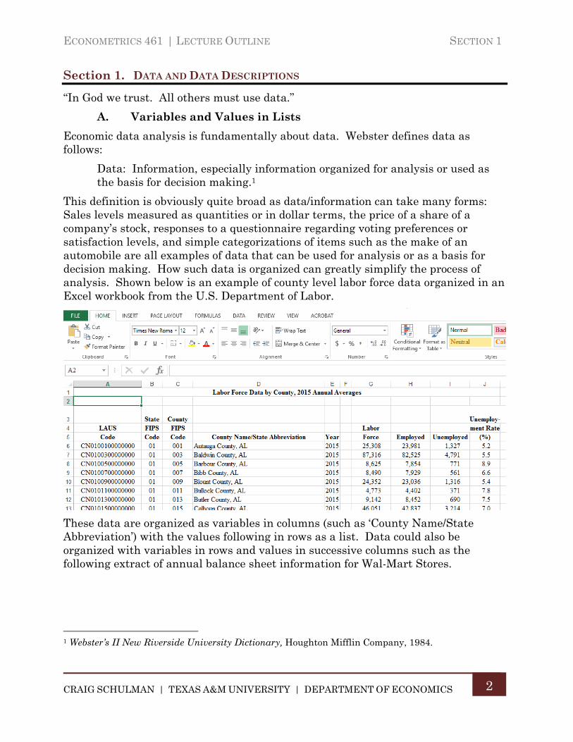
This definition is obviously quite broad as data/information can take many forms: Sales levels measured as quantities or in dollar terms, the price of a share of a company’s stock, responses to a questionnaire regarding voting preferences or satisfaction levels, and simple categorizations of items such as the make of an automobile are all examples of data that can be used for analysis or as a basis for decision making. How such data is organized can greatly simplify the process of analysis. Shown below is an example of county level labor force data organized in an Excel workbook from the U.S. Department of Labor.
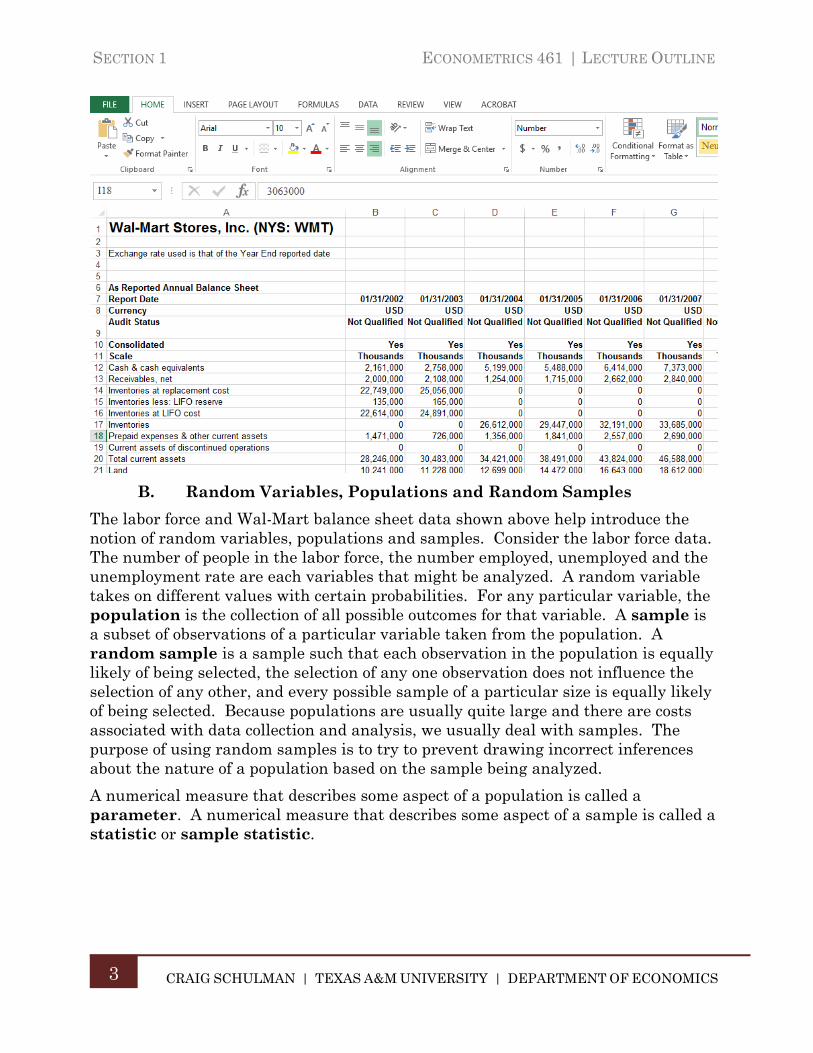
These data are organized as variables in columns (such as ‘County Name/State Abbreviation’) with the values following in rows as a list. Data could also be organized with variables in rows and values in successive columns such as the following extract of annual balance sheet information for Wal-Mart Stores.
1 Webster’s II New Riverside University Dictionary, Houghton Mifflin Company, 1984.
SECTION 1 ECONOMETRICS 461 | LECTURE OUTLINE
CRAIG SCHULMAN | TEXAS A&M UNIVERSITY | DEPARTMENT OF ECONOMICS
3
B. Random Variables, Populations and Random Samples
The labor force and Wal-Mart balance sheet data shown above help introduce the notion of random variables, populations and samples. Consider the labor force data. The number of people in the labor force, the number employed, unemployed and the unemployment rate are each variables that might be analyzed. A random variable takes on different values with certain probabilities. For any particular variable, the population is the collection of all possible outcomes for that variable. A sample is a subset of observations of a particular variable taken from the population. A random sample is a sample such that each observation in the population is equally likely of being selected, the selection of any one observation does not influence the selection of any other, and every possible sample of a particular size is equally likely of being selected. Because populations are usually quite large and there are costs associated with data collection and analysis, we usually deal with samples. The purpose of using random samples is to try to prevent drawing incorrect inferences about the nature of a population based on the sample being analyzed.
A numerical measure that describes some aspect of a population is called a parameter. A numerical measure that describes some aspect of a sample is called a statistic or sample statistic.
ECONOMETRICS 461 | LECTURE OUTLINE SECTION 1
CRAIG SCHULMAN | TEXAS A&M UNIVERSITY | DEPARTMENT OF ECONOMICS
4
C. Scales of Measurement – Data Types
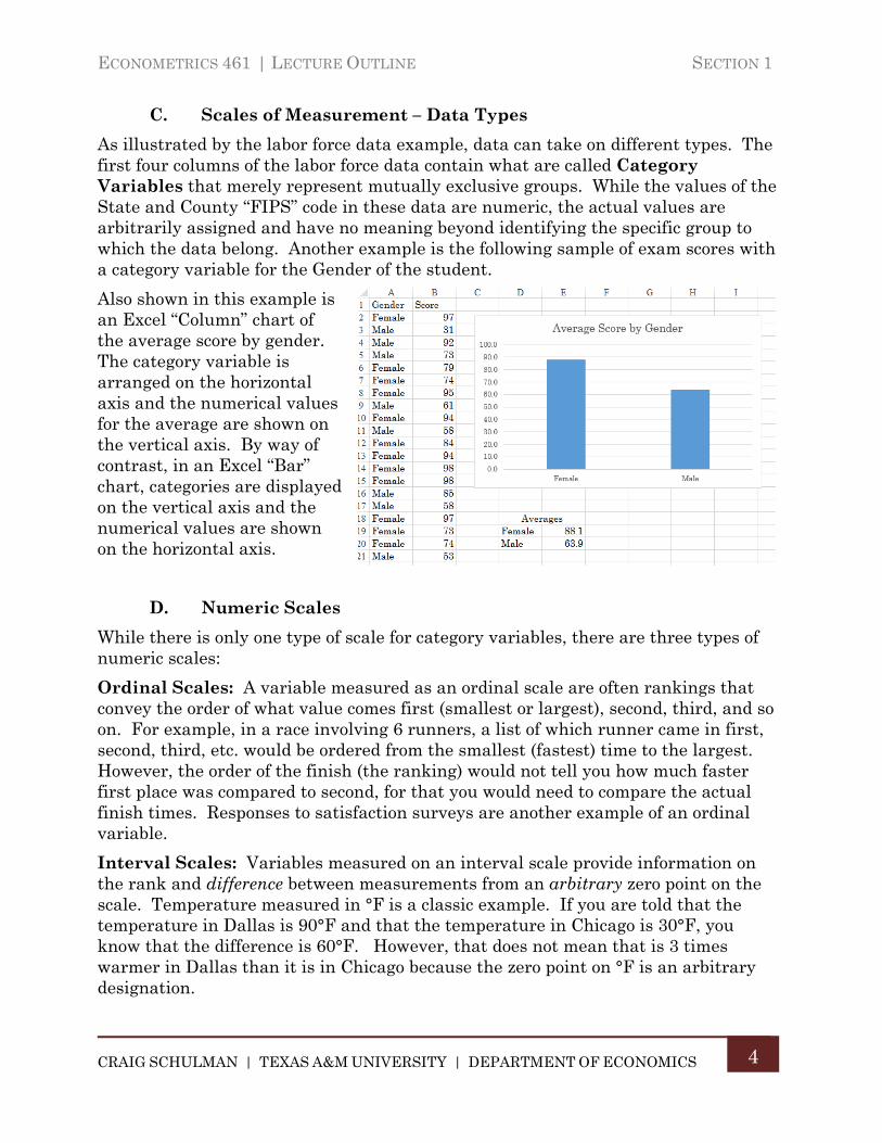
As illustrated by the labor force data example, data can take on different types. The first four columns of the labor force data contain what are called Category Variables that merely represent mutually exclusive groups. While the values of the State and County “FIPS” code in these data are numeric, the actual values are arbitrarily assigned and have no meaning beyond identifying the specific group to which the data belong. Another example is the following sample of exam scores with a category variable for the Gender of the student.
Also shown in this example is an Excel “Column” chart of the average score by gender. The category variable is arranged on the horizontal axis and the numerical values for the average are shown on the vertical axis. By way of contrast, in an Excel “Bar” chart, categories are displayed on the vertical axis and the numerical values are shown on the horizontal axis.
D. Numeric Scales
While there is only one type of scale for category variables, there are three types of numeric scales:
Ordinal Scales: A variable measured as an ordinal scale are often rankings that convey the order of what value comes first (smallest or largest), second, third, and so on. For example, in a race involving 6 runners, a list of which runner came in first, second, third, etc. would be ordered from the smallest (fastest) time to the largest. However, the order of the finish (the ranking) would not tell you how much faster first place was compared to second, for that you would need to compare the actual finish times. Responses to satisfaction surveys are another example of an ordinal variable.
Interval Scales: Variables measured on an interval scale provide information on the rank and difference between measurements from an arbitrary zero point on the scale. Temperature measured in °F is a classic example. If you are told that the temperature in Dallas is 90°F and that the temperature in Chicago is 30°F, you know that the difference is 60°F. However, that does not mean that is 3 times warmer in Dallas than it is in Chicago because the zero point on °F is an arbitrary designation.
SECTION 1 ECONOMETRICS 461 | LECTURE OUTLINE
CRAIG SCHULMAN | TEXAS A&M UNIVERSITY | DEPARTMENT OF ECONOMICS
5
Ratio Scales: Variables measured on a ratio scale provide information on the rank and distance from a natural zero point, with the ratio of two values having meaning. A person that is 50 years old is twice the age of someone who is 25. If per capita personal income in Mississippi is $35,000 and in Texas it is $47,000 personal income in Texas is about 34% higher than that in Mississippi.
E. Graphs to Describe Data
Categorical variables can be described with frequency tables and graphs such as bar charts and pie charts. These types of graphs are quite simple to construct and can provide a very powerful visual description of the underlying data.
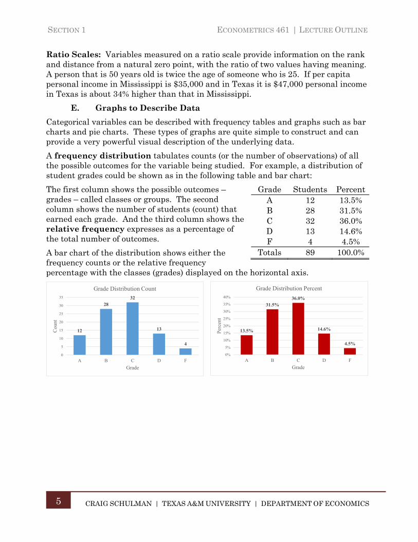
A frequency distribution tabulates counts (or the number of observations) of all the possible outcomes for the variable being studied. For example, a distribution of student grades could be shown as in the following table and bar chart:
The first column shows the possible outcomes – grades – called classes or groups. The second column shows the number of students (count) that earned each grade. And the third column shows the relative frequency expresses as a percentage of the total number of outcomes.
A bar chart of the distribution shows either the frequency counts or the relative frequency percentage with the classes (grades) displayed on the horizontal axis.
13.5%
31.5%36.0%
14.6%
4.5%
0%
5%
10%
15%
20%
25%
30%
35%
40%
A B C D F
Per
cent
Grade
Grade Distribution Percent
Grade Students Percent A 12 13.5% B 28 31.5% C 32 36.0% D 13 14.6% F 4 4.5%
Totals 89 100.0%
12
2832
13
4
0
5
10
15
20
25
30
35
A B C D F
Cou
nt
Grade
Grade Distribution Count
ECONOMETRICS 461 | LECTURE OUTLINE SECTION 1
CRAIG SCHULMAN | TEXAS A&M UNIVERSITY | DEPARTMENT OF ECONOMICS
6
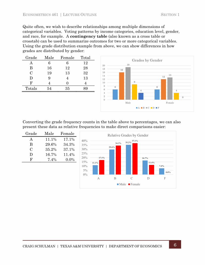
Quite often, we wish to describe relationships among multiple dimensions of categorical variables. Voting patterns by income categories, education level, gender, and race, for example. A contingency table (also known as a cross table or crosstab) can be used to summarize outcomes for two or more categorical variables. Using the grade distribution example from above, we can show differences in how grades are distributed by gender:
Converting the grade frequency counts in the table above to percentages, we can also present these data as relative frequencies to make direct comparisons easier:
11.1%
29.6%
35.2%
16.7%
7.4%
17.1%
34.3%37.1%
11.4%
0.0%0%5%
10%15%20%25%30%35%40%
A B C D F
Relative Grades by Gender
Male Female
Grade Male Female Total A 6 6 12 B 16 12 28 C 19 13 32 D 9 4 13 F 4 0 4
Totals 54 35 89
Grade Male Female A 11.1% 17.1% B 29.6% 34.3% C 35.2% 37.1% D 16.7% 11.4% F 7.4% 0.0%
6 6
16
12
19
13
9
44
002468
101214161820
Male Female
Grades by Gender
A B C D F
SECTION 1 ECONOMETRICS 461 | LECTURE OUTLINE
CRAIG SCHULMAN | TEXAS A&M UNIVERSITY | DEPARTMENT OF ECONOMICS
7
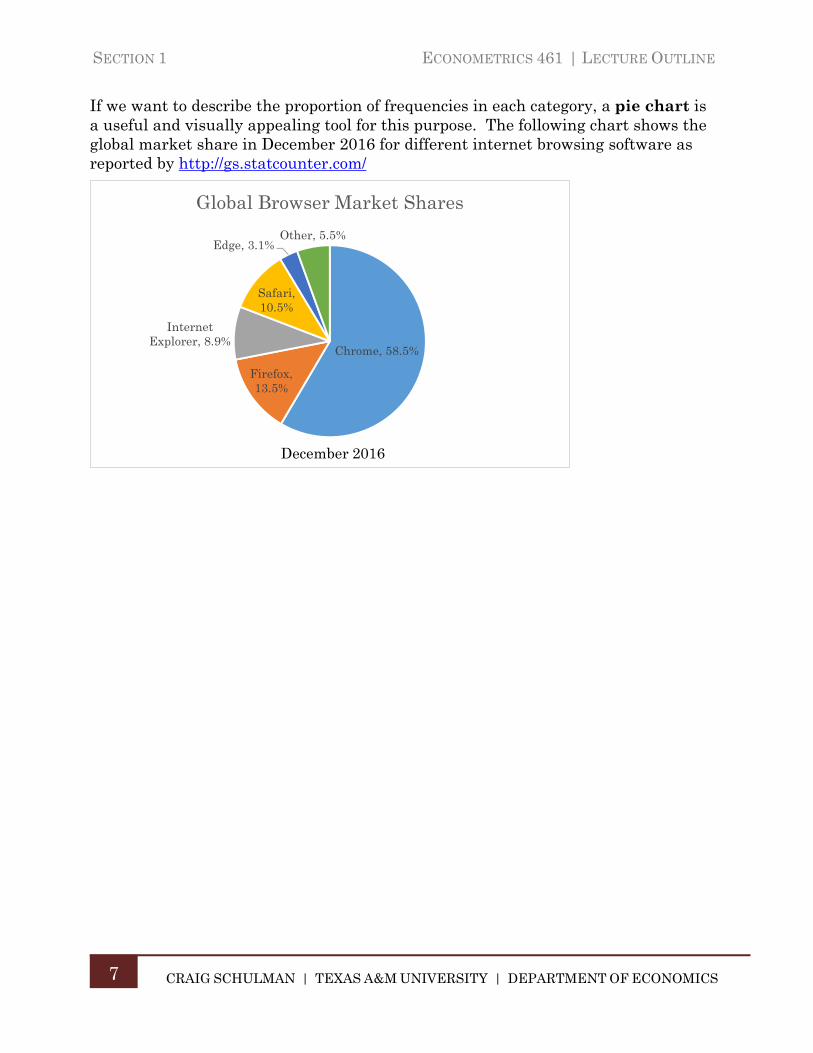
If we want to describe the proportion of frequencies in each category, a pie chart is a useful and visually appealing tool for this purpose. The following chart shows the global market share in December 2016 for different internet browsing software as reported by http://gs.statcounter.com/
Chrome, 58.5%
Firefox, 13.5%
Internet Explorer, 8.9%
Safari, 10.5%
Edge, 3.1%Other, 5.5%
Global Browser Market Shares
December 2016
ECONOMETRICS 461 | LECTURE OUTLINE SECTION 1
CRAIG SCHULMAN | TEXAS A&M UNIVERSITY | DEPARTMENT OF ECONOMICS
8
Time Series Data
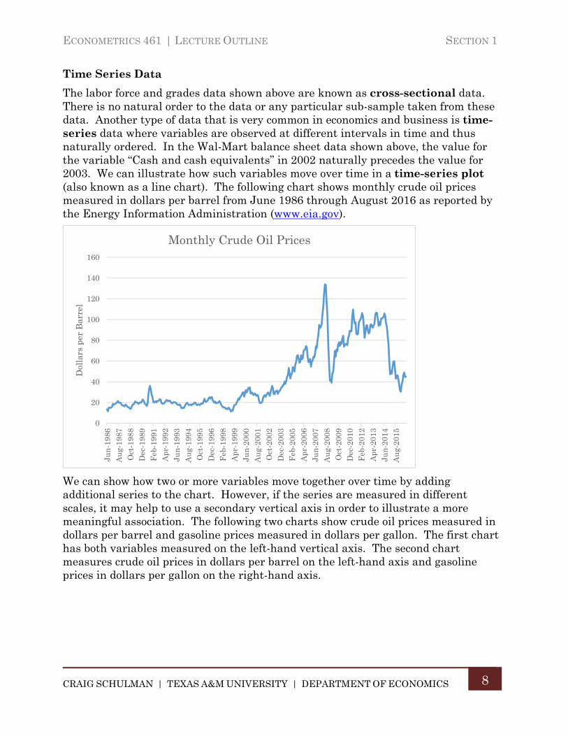
The labor force and grades data shown above are known as cross-sectional data. There is no natural order to the data or any particular sub-sample taken from these data. Another type of data that is very common in economics and business is time-series data where variables are observed at different intervals in time and thus naturally ordered. In the Wal-Mart balance sheet data shown above, the value for the variable “Cash and cash equivalents” in 2002 naturally precedes the value for 2003. We can illustrate how such variables move over time in a time-series plot (also known as a line chart). The following chart shows monthly crude oil prices measured in dollars per barrel from June 1986 through August 2016 as reported by the Energy Information Administration (www.eia.gov).
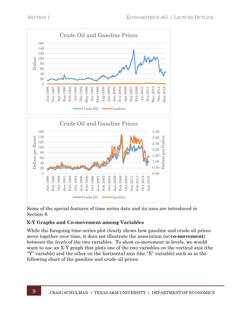
We can show how two or more variables move together over time by adding additional series to the chart. However, if the series are measured in different scales, it may help to use a secondary vertical axis in order to illustrate a more meaningful association. The following two charts show crude oil prices measured in dollars per barrel and gasoline prices measured in dollars per gallon. The first chart has both variables measured on the left-hand vertical axis. The second chart measures crude oil prices in dollars per barrel on the left-hand axis and gasoline prices in dollars per gallon on the right-hand axis.
0
20
40
60
80
100
120
140
160
Jun-
1986
Au
g-19
87O
ct-1
988
Dec
-198
9F
eb-1
991
Apr
-199
2
Jun-
1993
Au
g-19
94O
ct-1
995
Dec
-199
6
Feb
-199
8A
pr-1
999
Jun-
2000
Au
g-20
01O
ct-2
002
Dec
-200
3F
eb-2
005
Apr
-200
6Ju
n-20
07
Au
g-20
08O
ct-2
009
Dec
-201
0F
eb-2
012
Apr
-201
3Ju
n-20
14A
ug-
2015
Dol
lars
per
Bar
rel
Monthly Crude Oil Prices
SECTION 1 ECONOMETRICS 461 | LECTURE OUTLINE
CRAIG SCHULMAN | TEXAS A&M UNIVERSITY | DEPARTMENT OF ECONOMICS
9
Some of the special features of time series data and its uses are introduced in Section 8.
X-Y Graphs and Co-movement among Variables
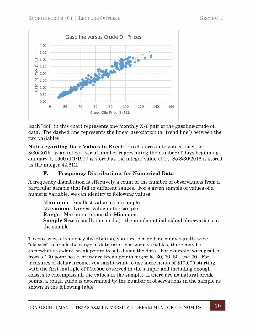
While the foregoing time-series plot clearly shows how gasoline and crude oil prices move together over time, it does not illustrate the association (or co-movement) between the levels of the two variables. To show co-movement in levels, we would want to use an X-Y graph that plots one of the two variables on the vertical axis (the “Y” variable) and the other on the horizontal axis (the “X” variable) such as in the following chart of the gasoline and crude oil prices:
020406080
100120140160
Jun-
1986
Nov
-198
7
Apr
-198
9
Sep
-199
0
Feb
-199
2
Jul-
1993
Dec
-199
4
May
-199
6
Oct
-199
7
Mar
-199
9
Au
g-20
00
Jan
-200
2
Jun-
2003
Nov
-200
4
Apr
-200
6
Sep
-200
7
Feb
-200
9
Jul-
2010
Dec
-201
1
May
-201
3
Oct
-201
4
Mar
-201
6
Dol
lars
Crude Oil and Gasoline Prices
Crude Oil Gasoline
0.00
0.50
1.00
1.50
2.00
2.50
3.00
3.50
020406080
100120140160
Jun-
1986
Feb
-198
8
Oct
-198
9
Jun-
1991
Feb
-199
3
Oct
-199
4
Jun-
1996
Feb
-199
8
Oct
-199
9
Jun-
2001
Feb
-200
3
Oct
-200
4
Jun-
2006
Feb
-200
8
Oct
-200
9
Jun-
2011
Feb
-201
3
Oct
-201
4
Jun-
2016
Dol
lars
per
Gal
lon
Dol
lars
per
Bar
rel
Crude Oil and Gasoline Prices
Crude Oil Gasoline
ECONOMETRICS 461 | LECTURE OUTLINE SECTION 1
CRAIG SCHULMAN | TEXAS A&M UNIVERSITY | DEPARTMENT OF ECONOMICS
10
Each “dot” in this chart represents one monthly X-Y pair of the gasoline-crude oil data. The dashed line represents the linear association (a “trend line”) between the two variables.
Note regarding Date Values in Excel: Excel stores date values, such as 8/30/2016, as an integer serial number representing the number of days beginning January 1, 1900 (1/1/1900 is stored as the integer value of 1). So 8/30/2016 is stored as the integer 42,612.
F. Frequency Distributions for Numerical Data
A frequency distribution is effectively a count of the number of observations from a particular sample that fall in different ranges. For a given sample of values of a numeric variable, we can identify to following values:
Minimum: Smallest value in the sample Maximum: Largest value in the sample Range: Maximum minus the Minimum Sample Size (usually denoted n): the number of individual observations in the sample.
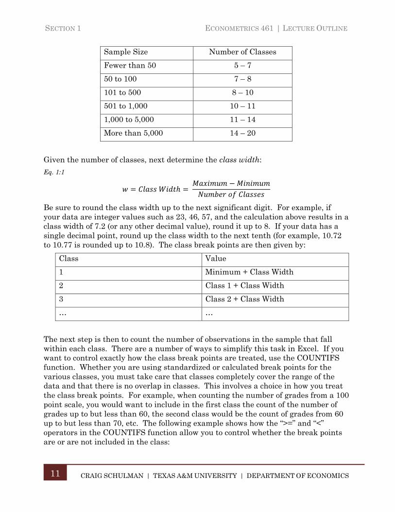
To construct a frequency distribution, you first decide how many equally wide “classes” to break the range of data into. For some variables, there may be somewhat standard break points to sub-divide the data. For example, with grades from a 100 point scale, standard break points might be 60, 70, 80, and 90. For measures of dollar income, you might want to use increments of $10,000 starting with the first multiple of $10,000 observed in the sample and including enough classes to encompass all the values in the sample. If there are no natural break points, a rough guide is determined by the number of observations in the sample as shown in the following table:
0.00
0.50
1.00
1.50
2.00
2.50
3.00
3.50
4.00
0 20 40 60 80 100 120 140 160
Gasolin
e Price ($/G
al)
Crude Oile Price ($/BBL)
Gasoline versus Crude Oil Prices
SECTION 1 ECONOMETRICS 461 | LECTURE OUTLINE
CRAIG SCHULMAN | TEXAS A&M UNIVERSITY | DEPARTMENT OF ECONOMICS
11
Sample Size Number of Classes
Fewer than 50 5 – 7
50 to 100 7 – 8
101 to 500 8 – 10
501 to 1,000 10 – 11
1,000 to 5,000 11 – 14
More than 5,000 14 – 20
Given the number of classes, next determine the class width:
Eq. 1:1
Be sure to round the class width up to the next significant digit. For example, if your data are integer values such as 23, 46, 57, and the calculation above results in a class width of 7.2 (or any other decimal value), round it up to 8. If your data has a single decimal point, round up the class width to the next tenth (for example, 10.72 to 10.77 is rounded up to 10.8). The class break points are then given by:
Class Value
1 Minimum + Class Width
2 Class 1 + Class Width
3 Class 2 + Class Width
… …
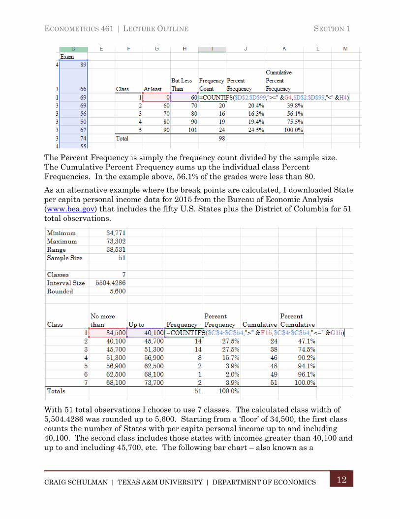
The next step is then to count the number of observations in the sample that fall within each class. There are a number of ways to simplify this task in Excel. If you want to control exactly how the class break points are treated, use the COUNTIFS function. Whether you are using standardized or calculated break points for the various classes, you must take care that classes completely cover the range of the data and that there is no overlap in classes. This involves a choice in how you treat the class break points. For example, when counting the number of grades from a 100 point scale, you would want to include in the first class the count of the number of grades up to but less than 60, the second class would be the count of grades from 60 up to but less than 70, etc. The following example shows how the “>=” and “<” operators in the COUNTIFS function allow you to control whether the break points are or are not included in the class:
ECONOMETRICS 461 | LECTURE OUTLINE SECTION 1
CRAIG SCHULMAN | TEXAS A&M UNIVERSITY | DEPARTMENT OF ECONOMICS
12
The Percent Frequency is simply the frequency count divided by the sample size. The Cumulative Percent Frequency sums up the individual class Percent Frequencies. In the example above, 56.1% of the grades were less than 80.
As an alternative example where the break points are calculated, I downloaded State per capita personal income data for 2015 from the Bureau of Economic Analysis (www.bea.gov) that includes the fifty U.S. States plus the District of Columbia for 51 total observations.
With 51 total observations I choose to use 7 classes. The calculated class width of 5,504.4286 was rounded up to 5,600. Starting from a ‘floor’ of 34,500, the first class counts the number of States with per capita personal income up to and including 40,100. The second class includes those states with incomes greater than 40,100 and up to and including 45,700, etc. The following bar chart – also known as a
SECTION 1 ECONOMETRICS 461 | LECTURE OUTLINE
CRAIG SCHULMAN | TEXAS A&M UNIVERSITY | DEPARTMENT OF ECONOMICS
13
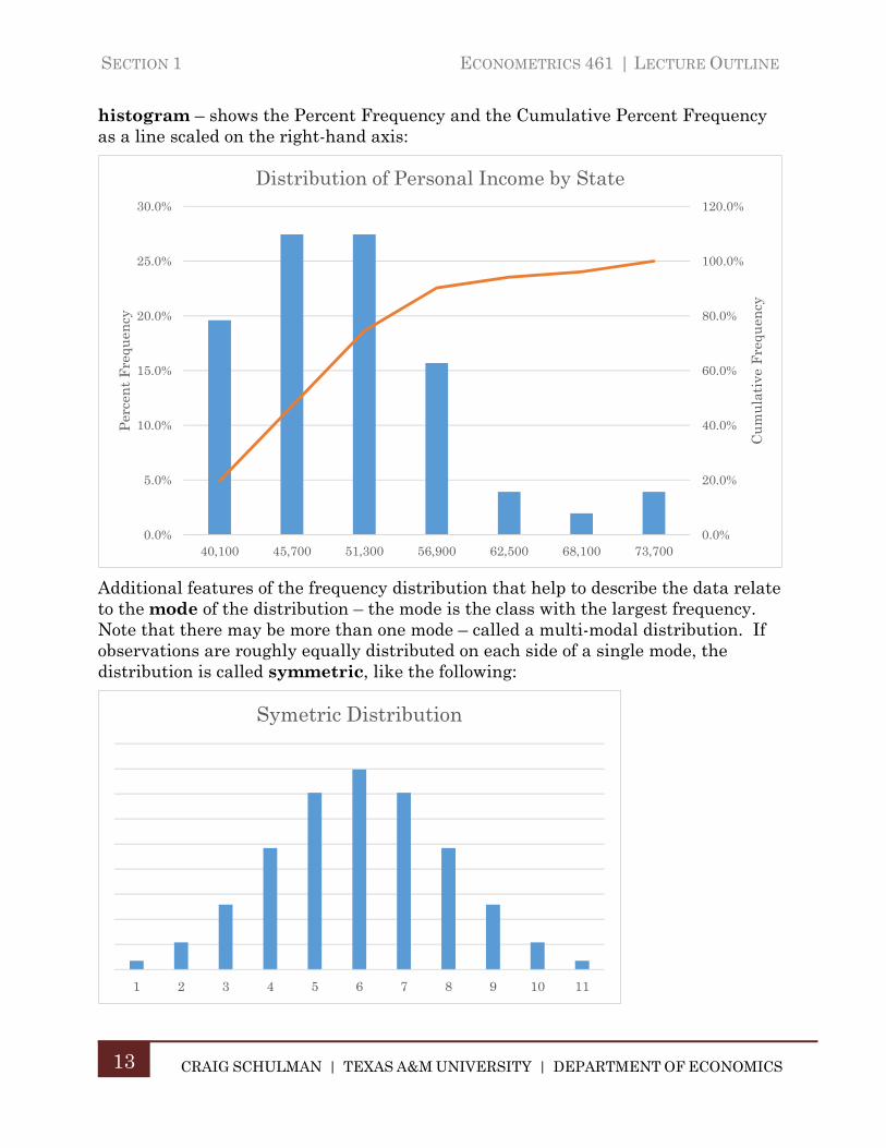
histogram – shows the Percent Frequency and the Cumulative Percent Frequency as a line scaled on the right-hand axis:
Additional features of the frequency distribution that help to describe the data relate to the mode of the distribution – the mode is the class with the largest frequency. Note that there may be more than one mode – called a multi-modal distribution. If observations are roughly equally distributed on each side of a single mode, the distribution is called symmetric, like the following:
0.0%
20.0%
40.0%
60.0%
80.0%
100.0%
120.0%
0.0%
5.0%
10.0%
15.0%
20.0%
25.0%
30.0%
40,100 45,700 51,300 56,900 62,500 68,100 73,700
Cu
mu
lati
ve F
requ
ency
Per
cen
t F
requ
ency
Distribution of Personal Income by State
1 2 3 4 5 6 7 8 9 10 11
Symetric Distribution
ECONOMETRICS 461 | LECTURE OUTLINE SECTION 1
CRAIG SCHULMAN | TEXAS A&M UNIVERSITY | DEPARTMENT OF ECONOMICS
14
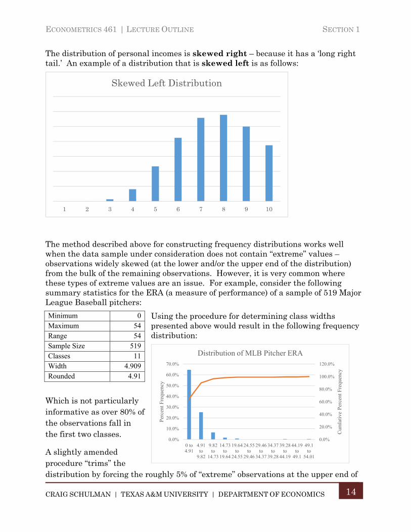
The distribution of personal incomes is skewed right – because it has a ‘long right tail.’ An example of a distribution that is skewed left is as follows:
The method described above for constructing frequency distributions works well when the data sample under consideration does not contain “extreme” values – observations widely skewed (at the lower and/or the upper end of the distribution) from the bulk of the remaining observations. However, it is very common where these types of extreme values are an issue. For example, consider the following summary statistics for the ERA (a measure of performance) of a sample of 519 Major League Baseball pitchers:
Using the procedure for determining class widths presented above would result in the following frequency distribution:
Which is not particularly informative as over 80% of the observations fall in the first two classes.
A slightly amended procedure “trims” the distribution by forcing the roughly 5% of “extreme” observations at the upper end of
1 2 3 4 5 6 7 8 9 10
Skewed Left Distribution
Minimum 0 Maximum 54 Range 54 Sample Size 519 Classes 11 Width 4.909 Rounded 4.91
0.0%
20.0%
40.0%
60.0%
80.0%
100.0%
120.0%
0.0%
10.0%
20.0%
30.0%
40.0%
50.0%
60.0%
70.0%
0 to4.91
4.91to
9.82
9.82to
14.73
14.73to
19.64
19.64to
24.55
24.55to
29.46
29.46to
34.37
34.37to
39.28
39.28to
44.19
44.19to
49.1
49.1to
54.01
Cum
lativ
e P
erce
nt F
requ
ency
Per
cent
Fre
quen
cy
Distribution of MLB Pitcher ERA
SECTION 1 ECONOMETRICS 461 | LECTURE OUTLINE
CRAIG SCHULMAN | TEXAS A&M UNIVERSITY | DEPARTMENT OF ECONOMICS
15
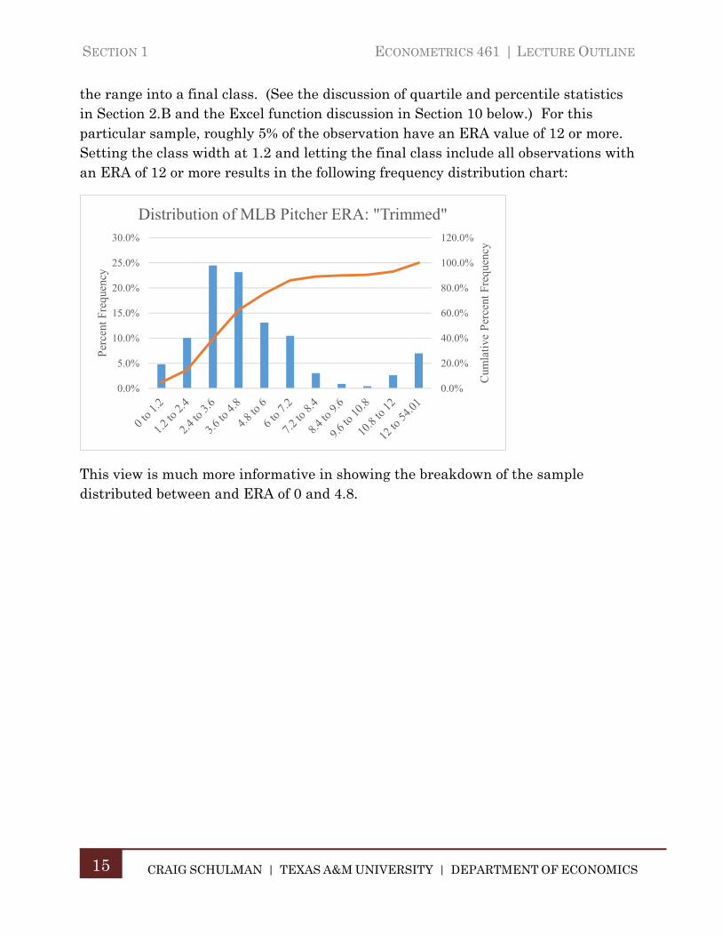
the range into a final class. (See the discussion of quartile and percentile statistics in Section 2.B and the Excel function discussion in Section 10 below.) For this particular sample, roughly 5% of the observation have an ERA value of 12 or more. Setting the class width at 1.2 and letting the final class include all observations with an ERA of 12 or more results in the following frequency distribution chart:
This view is much more informative in showing the breakdown of the sample distributed between and ERA of 0 and 4.8.
0.0%
20.0%
40.0%
60.0%
80.0%
100.0%
120.0%
0.0%
5.0%
10.0%
15.0%
20.0%
25.0%
30.0%
Cum
lati
ve P
erce
nt F
requ
ency
Per
cent
Fre
quen
cy
Distribution of MLB Pitcher ERA: "Trimmed"
ECONOMETRICS 461 | LECTURE OUTLINE SECTION 1
CRAIG SCHULMAN | TEXAS A&M UNIVERSITY | DEPARTMENT OF ECONOMICS
16
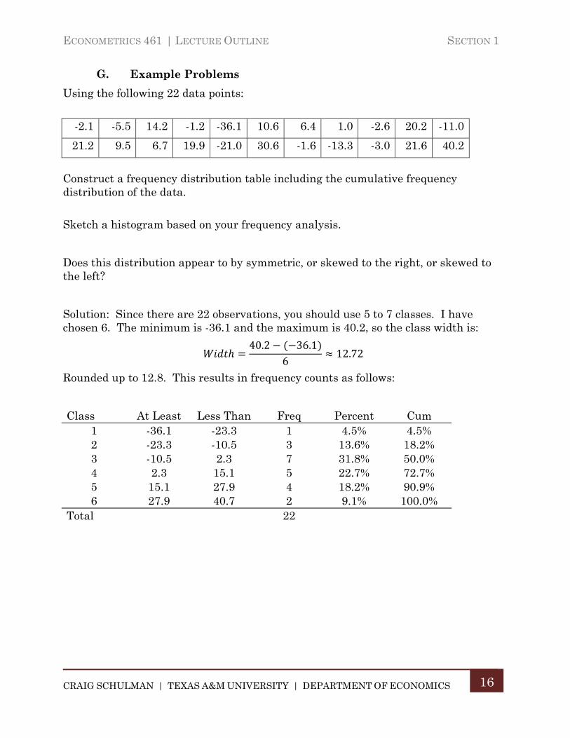
G. Example Problems
Using the following 22 data points:
-2.1 -5.5 14.2 -1.2 -36.1 10.6 6.4 1.0 -2.6 20.2 -11.0
21.2 9.5 6.7 19.9 -21.0 30.6 -1.6 -13.3 -3.0 21.6 40.2
Construct a frequency distribution table including the cumulative frequency distribution of the data.
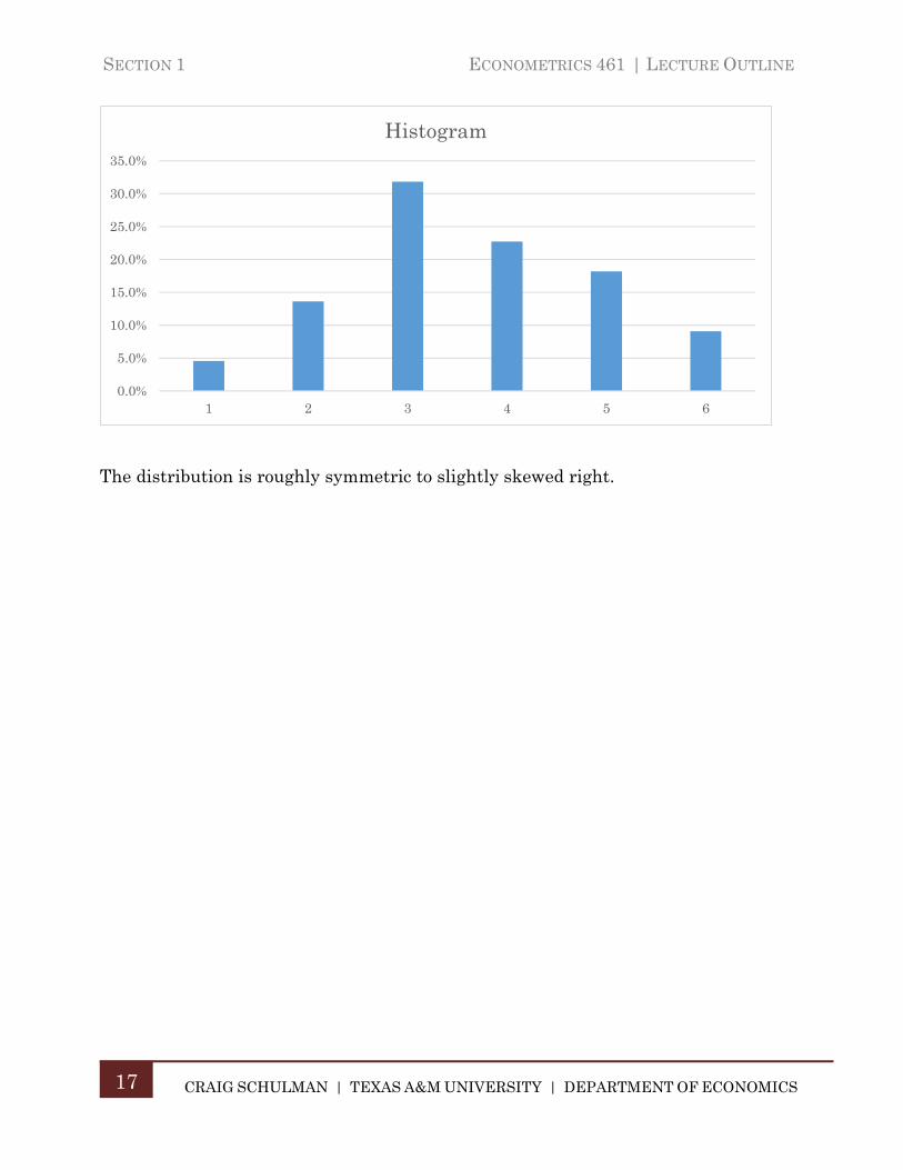
Sketch a histogram based on your frequency analysis.
Does this distribution appear to by symmetric, or skewed to the right, or skewed to the left?
Solution: Since there are 22 observations, you should use 5 to 7 classes. I have chosen 6. The minimum is -36.1 and the maximum is 40.2, so the class width is:
40.2 36.16
12.72
Rounded up to 12.8. This results in frequency counts as follows:
Class At Least Less Than Freq Percent Cum 1 -36.1 -23.3 1 4.5% 4.5% 2 -23.3 -10.5 3 13.6% 18.2% 3 -10.5 2.3 7 31.8% 50.0% 4 2.3 15.1 5 22.7% 72.7% 5 15.1 27.9 4 18.2% 90.9% 6 27.9 40.7 2 9.1% 100.0%
Total 22
SECTION 1 ECONOMETRICS 461 | LECTURE OUTLINE
CRAIG SCHULMAN | TEXAS A&M UNIVERSITY | DEPARTMENT OF ECONOMICS
17
The distribution is roughly symmetric to slightly skewed right.
0.0%
5.0%
10.0%
15.0%
20.0%
25.0%
30.0%
35.0%
1 2 3 4 5 6
Histogram
ECONOMETRICS 461 | LECTURE OUTLINE SECTION 2
CRAIG SCHULMAN | TEXAS A&M UNIVERSITY | DEPARTMENT OF ECONOMICS
18
Section 2. MEASURES OF CENTRAL TENDENCY, VARIABILITY AND CO-MOVEMENT
In analyzing any particular numerical variable, the frequency distributions we explored in Section1 help illustrate that with many economic variables, certain values (or ranges of values) are observed more frequently than others. Ultimately, we want to be able to make statements in probability about the likelihood of a particular variable taking on either a specific value or a value in specific range. For a single variable, this will require constructing measures that help indicate whether observations are centered or clustered around a particular value and the degree to which observations deviate around that central value. These are called measures of central tendency and variability. When two or more variables are the focus of the analysis, we will examine measures of co-movement that provide an indication of how observations my cluster together.
A. Measures of Central Tendency
For a sample of a single random variable, measures of central tendency provide a single value for the “center” of the data. We will examine three different measures of central tendency: the mean, median and mode. In addition, we will examine three different types of measures of the mean: the arithmetic mean, the weighted mean, and the geometric mean.
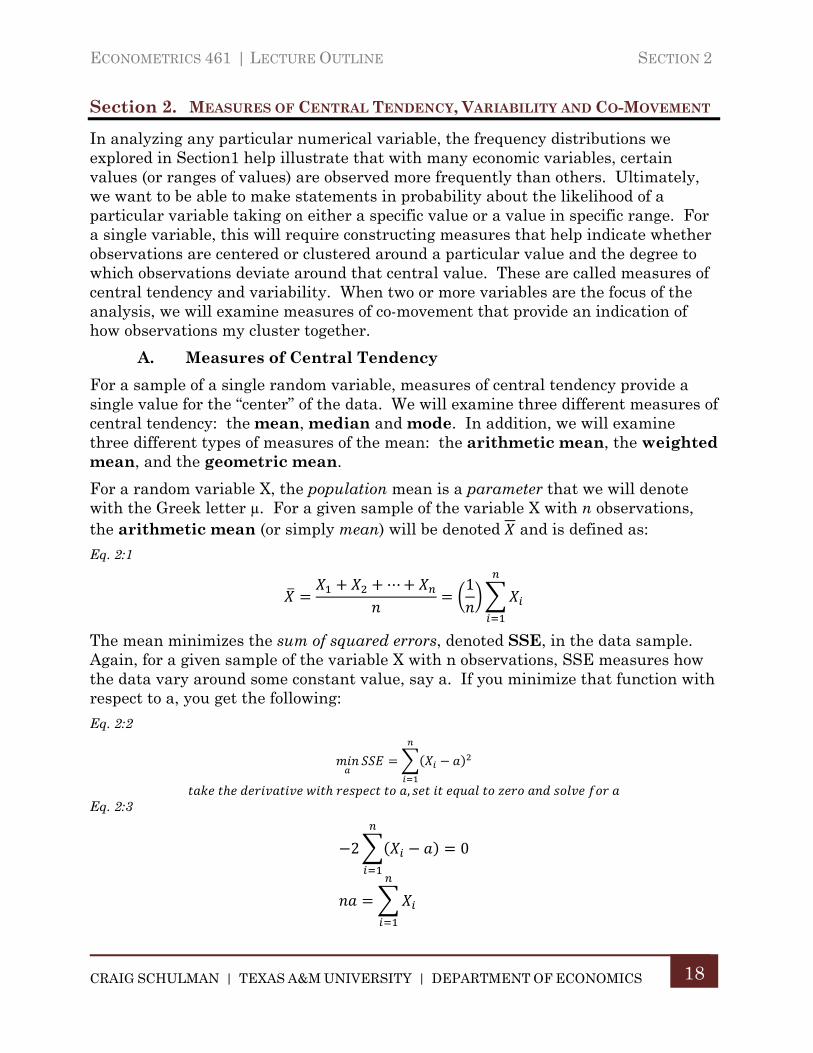
For a random variable X, the population mean is a parameter that we will denote with the Greek letter µ. For a given sample of the variable X with n observations, the arithmetic mean (or simply mean) will be denoted and is defined as:
Eq. 2:1
⋯ 1
The mean minimizes the sum of squared errors, denoted SSE, in the data sample. Again, for a given sample of the variable X with n observations, SSE measures how the data vary around some constant value, say a. If you minimize that function with respect to a, you get the following:
Eq. 2:2
, Eq. 2:3
2 0
SECTION 2 ECONOMETRICS 461 | LECTURE OUTLINE
CRAIG SCHULMAN | TEXAS A&M UNIVERSITY | DEPARTMENT OF ECONOMICS
19
1
Note: You will not be required to derive the minimum SSE result above. However, we will see the notion of minimum SSE statistics throughout the semester and you will see this concept again in detail in your Econometrics 463 course.
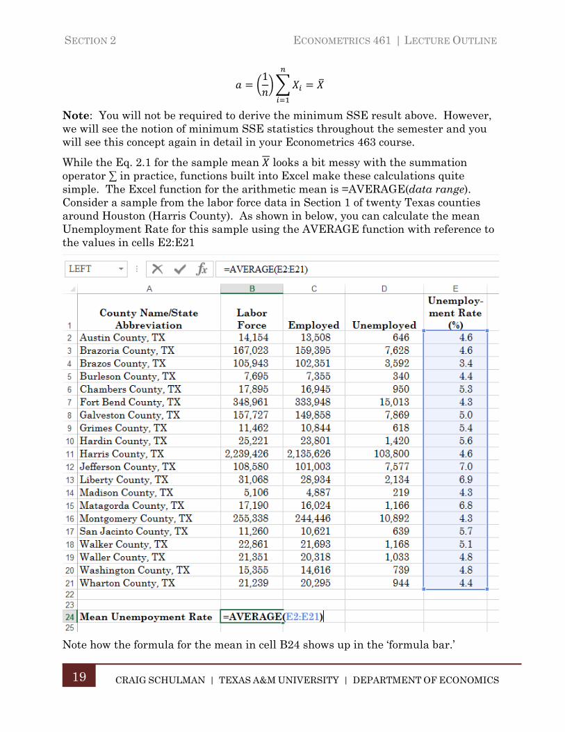
While the Eq. 2.1 for the sample mean looks a bit messy with the summation operator ∑ in practice, functions built into Excel make these calculations quite simple. The Excel function for the arithmetic mean is =AVERAGE(data range). Consider a sample from the labor force data in Section 1 of twenty Texas counties around Houston (Harris County). As shown in below, you can calculate the mean Unemployment Rate for this sample using the AVERAGE function with reference to the values in cells E2:E21
Note how the formula for the mean in cell B24 shows up in the ‘formula bar.’
ECONOMETRICS 461 | LECTURE OUTLINE SECTION 2
CRAIG SCHULMAN | TEXAS A&M UNIVERSITY | DEPARTMENT OF ECONOMICS
20
Effect of changing scale on the Sample Mean: If you rescale a variable – by multiplying and/or adding a constant – this will affect the calculated value of the sample mean. For example, suppose an instructor gives an exam worth a total of 60 points and the mean score is 43. If scores are rescaled to a 100 point basis by multiplying by 10/6, and the instructor then applies a curve by adding 4 points, what is the new mean score? To see the solution, let the original set of scores be represented by the variable X, let a and b be constants, and let the rescaled scores be represented by the variable Y with: Y . Then,
Eq. 2:4
Applying this formula to the exam example, the new mean score is about 75.67.
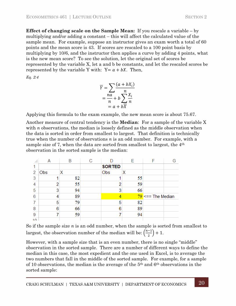
Another measure of central tendency is the Median: For a sample of the variable X with n observations, the median is loosely defined as the middle observation when the data is sorted in order from smallest to largest. That definition is technically true when the number of observations n is an odd number. For example, with a sample size of 7, when the data are sorted from smallest to largest, the 4th observation in the sorted sample is the median:
So if the sample size n is an odd number, when the sample is sorted from smallest to largest, the observation number of the median will be: 1.
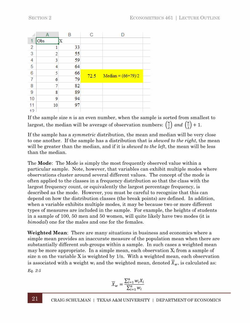
However, with a sample size that is an even number, there is no single “middle” observation in the sorted sample. There are a number of different ways to define the median in this case, the most expedient and the one used in Excel, is to average the two numbers that fall in the middle of the sorted sample. For example, for a sample of 10 observations, the median is the average of the 5th and 6th observations in the sorted sample:
SECTION 2 ECONOMETRICS 461 | LECTURE OUTLINE
CRAIG SCHULMAN | TEXAS A&M UNIVERSITY | DEPARTMENT OF ECONOMICS
21
If the sample size n is an even number, when the sample is sorted from smallest to largest, the median will be average of observation numbers: 1.
If the sample has a symmetric distribution, the mean and median will be very close to one another. If the sample has a distribution that is skewed to the right, the mean will be greater than the median, and if it is skewed to the left, the mean will be less than the median.
The Mode: The Mode is simply the most frequently observed value within a particular sample. Note, however, that variables can exhibit multiple modes where observations cluster around several different values. The concept of the mode is often applied to the classes in a frequency distribution so that the class with the largest frequency count, or equivalently the largest percentage frequency, is described as the mode. However, you must be careful to recognize that this can depend on how the distribution classes (the break points) are defined. In addition, when a variable exhibits multiple modes, it may be because two or more different types of measures are included in the sample. For example, the heights of students in a sample of 100, 50 men and 50 women, will quite likely have two modes (it is bimodal) one for the males and one for the females.
Weighted Mean: There are many situations in business and economics where a simple mean provides an inaccurate measure of the population mean when there are substantially different sub-groups within a sample. In such cases a weighted mean may be more appropriate. In a simple mean, each observation Xi from a sample of size n on the variable X is weighted by 1/n. With a weighted mean, each observation is associated with a weight wi and the weighted mean, denoted , is calculated as:
Eq. 2:5
∑∑

ECONOMETRICS 461 | LECTURE OUTLINE SECTION 2
CRAIG SCHULMAN | TEXAS A&M UNIVERSITY | DEPARTMENT OF ECONOMICS
22
An example where a weighted mean would be appropriate is when you have summary measures on a number of groups (for example, unemployment rates for different counties) and the groups are different sizes (counties have different sized labor forces). For example, in the 20 county sample of labor force data shown above, the simple mean of the unemployment rate is 5.07. When rates are weighted by the size of the labor force, the weighted mean is 4.65. In this example, the weighted mean is less than the simple mean because the counties with the largest labor force tend to have unemployment rates less than that of the simple mean. It is straightforward to calculate a weighted mean in Excel using a combination of the SUMPRODUCT and SUM functions via: =SUMPRODUCT(range for weights, range for X values)/SUM(range for weights) such as the following:
Another specialize measure of central tendency is the Geometric Mean. The Geometric Mean, denoted , is a specialized average used in business and economics with growth rates and rates of return. Instead of adding the values in a sample and dividing by the sample size, the values are multiplied together (you take
SECTION 2 ECONOMETRICS 461 | LECTURE OUTLINE
CRAIG SCHULMAN | TEXAS A&M UNIVERSITY | DEPARTMENT OF ECONOMICS
23
the product of the series) and the nth root is applied to the result. The geometric mean of X for a sample of size n is given by:
Eq. 2:6
…
Where the Greek letter Π is used to denote the product of the values. If Xi is the periodic gross rate of growth between period i-1 and i: , then the geometric
mean measures the Average Compound Periodic Return, and the calculation simplifies to:
Eq. 2:7
You can calculate a geometric mean in Excel using the GEOMEAN(data range) function.
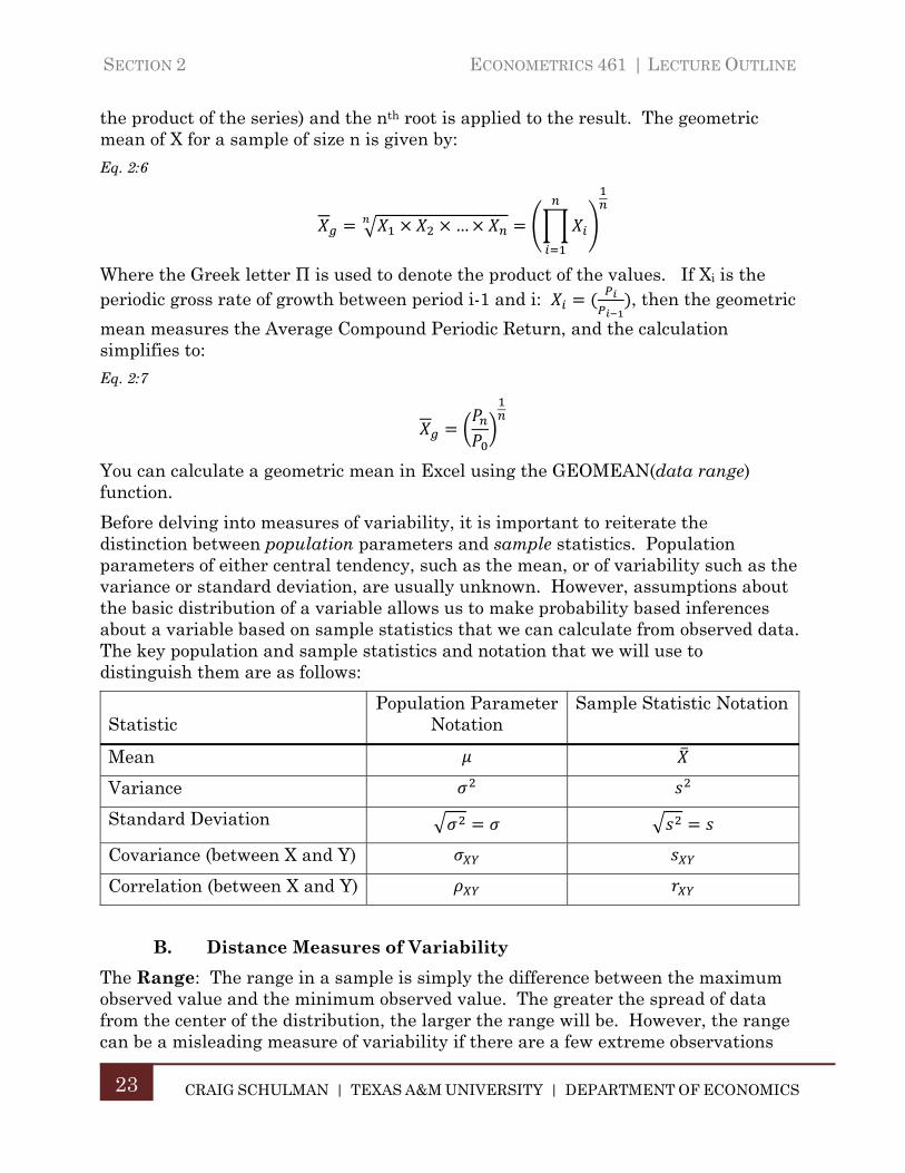
Before delving into measures of variability, it is important to reiterate the distinction between population parameters and sample statistics. Population parameters of either central tendency, such as the mean, or of variability such as the variance or standard deviation, are usually unknown. However, assumptions about the basic distribution of a variable allows us to make probability based inferences about a variable based on sample statistics that we can calculate from observed data. The key population and sample statistics and notation that we will use to distinguish them are as follows:
Statistic Population Parameter
Notation Sample Statistic Notation
Mean
Variance
Standard Deviation
Covariance (between X and Y)
Correlation (between X and Y)
B. Distance Measures of Variability
The Range: The range in a sample is simply the difference between the maximum observed value and the minimum observed value. The greater the spread of data from the center of the distribution, the larger the range will be. However, the range can be a misleading measure of variability if there are a few extreme observations
ECONOMETRICS 461 | LECTURE OUTLINE SECTION 2
CRAIG SCHULMAN | TEXAS A&M UNIVERSITY | DEPARTMENT OF ECONOMICS
24
(either very large or very small), called outliers. To control for this possibility, it is helpful to look at the range of the middle 50% of the data: the interquartile range.
Interquartile Range: The first quartile, denoted Q1, is the value below which 25% of the observations fall. The first quartile is also known as the 25th percentile. The third quartile, Q3, is the value below which 75% of the observations fall (a.k.a., the 75th percentile). The interquartile range is then: . Note that the second quartile, a.k.a. the 50th percentile, is the median. In practice, there are a number of different methods for calculating quartiles, none of which are absolutely definitive. Excel includes two different functions for calculating quartiles: QUARTILE.INC and QUARTILE.EXC (Excel also includes a ‘legacy’ function QUARTILE that is the same as QUARTILE.INC). For a number of reasons, I would suggest using the QUARTILE.EXC function. For more information on calculating quartiles see the blog post: http://datapigtechnologies.com/blog/index.php/why-excel-has-multiple-quartile-functions-and-how-to-replicate-the-quartiles-from-r-and-other-statistical-packages/ .
The PERCENTILE.EXC function is similar to the QUARTILE.EXC function. It returns the value in a data array below which any percentage between 0 and 1 of the sample fall. For example, PERCENTILE.EXC(array,0.9) returns the value in array below which 90% of the observations fall.
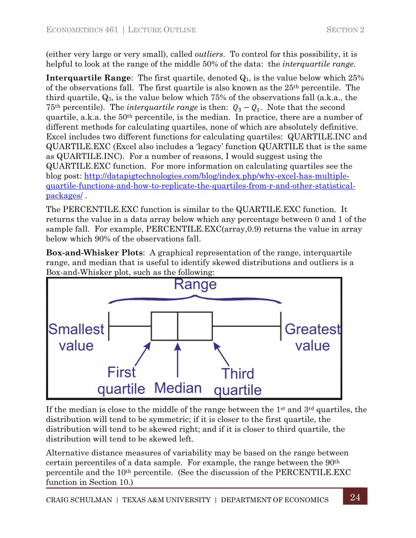
Box-and-Whisker Plots: A graphical representation of the range, interquartile range, and median that is useful to identify skewed distributions and outliers is a Box-and-Whisker plot, such as the following:
If the median is close to the middle of the range between the 1st and 3rd quartiles, the distribution will tend to be symmetric; if it is closer to the first quartile, the distribution will tend to be skewed right; and if it is closer to third quartile, the distribution will tend to be skewed left.
Alternative distance measures of variability may be based on the range between certain percentiles of a data sample. For example, the range between the 90th percentile and the 10th percentile. (See the discussion of the PERCENTILE.EXC function in Section 10.)
SECTION 2 ECONOMETRICS 461 | LECTURE OUTLINE
CRAIG SCHULMAN | TEXAS A&M UNIVERSITY | DEPARTMENT OF ECONOMICS
25
C. Variance and Standard Deviation
The preceding distance measures of variability all measure ranges based in specific pairs of observations in a sample. Variance and standard deviation statistics are averages of variability across all observations either in the population or in a particular sample. The population variance, , is the sum of the squared differences between each observation and the population mean, µ, divided by the population size N:
Eq. 2:8
∑
The sample variance, s2, is the sum of the squared differences between each observation and the sample mean, , divided by the sample size n, minus 1:
Eq. 2:9
∑
1
The (n – 1) in the denominator is called the degrees of freedom, and is used instead of simply the sample size to make the sample variance s2 an unbiased estimator of the population variance: that is, on average, s2 will equal the population variance. A computational shortcut that is handy if you are calculating a sample variance manually is as follows:
Eq. 2:10
∑
1
Standard deviation, for either the population or the sample, is the square root of the variance. Thus the population standard deviation is:
Eq. 2:11
∑
And the sample standard deviation is:
Eq. 2:12
∑1
ECONOMETRICS 461 | LECTURE OUTLINE SECTION 2
CRAIG SCHULMAN | TEXAS A&M UNIVERSITY | DEPARTMENT OF ECONOMICS
26
The Excel functions for variance and standard deviation are summarized in the following table.
Function Result
VAR.P Population variance – uses N in the denominator
VAR.S Sample variance – using n-1 in the denominator
STDEV.P Population standard deviation – the square root of VAR.P
STDEV.S Sample standard deviation – the square root of VAR.S
Changing Scales: If you add (or subtract) a constant from a variable X, there is NO effect on the variance or standard deviation since the mean will change by the same constant. However, if you multiply by a constant k, the resulting variance will be times the original variance, and the standard deviation will be k times the original standard deviation.
The importance of the standard deviation is illustrated by the Empirical Rule: for any variable that has approximately a normal bell-shaped distribution, approximately 68% if the observations will lie within the interval , approximately 96% of the observations will lie within the interval 2 , and almost all the observations will lie within the interval 3 .
Coefficient of Variation: With measures of the standard deviation on different variables, it may be tempting to make a direct comparison among the standard deviation statistics to address the question of which variable exhibits more or less variability about its mean. However, if the variables have different means, such a comparison does not have much meaning. To remove these scale effects, we can compare the coefficient of variation, denoted CV, which is the ratio of a variable’s standard deviation to its mean (either population of sample measures) provided the means are positive, and is usually expressed as a percentage. Thus, the population coefficient of variation is:
Eq. 2:13
And the sample coefficient of variation is:
Eq. 2:14
Z-Score: A z-score is a standardized value that indicates the number of standard deviations a specific data value is from the mean. It can be positive (value is greater than the mean) negative (value is less than the mean) or zero (equal to the mean):
SECTION 2 ECONOMETRICS 461 | LECTURE OUTLINE
CRAIG SCHULMAN | TEXAS A&M UNIVERSITY | DEPARTMENT OF ECONOMICS
27
Eq. 2:15
The z-score can also be calculated based on the sample measures of the mean and standard deviation:
Eq. 2:16
For a given sample, if all the observations are converted to z-scores, it is straightforward to show that the sample mean of the z-scores is zero and its standard deviation is one.
D. Measures of Co-Movement
The measures of central tendency discussed above help us understand how the observations of a random variance will cluster around a central point while measures of variability help us understand the extent of variation. We now turn to how two random variables tend to move together – or co-movement. The base measure of co-movement in a pair of random variables X and Y, is their covariance. The sample measure of the covariance between X and Y is:
Eq. 2:17
∑
1
The covariance provides a measure of the tendency of the variable X to move together with the variable Y. If the variable Y tends to increase at the same time that the variable X increases, the covariance will be positive. If Y tends to decrease as X increases, the covariance will be negative. Beyond the sign or direction of the relationship, however, the covariance is not very informative because it is subject to scale effects. If the variable X is multiplied by a constant kX, then the covariance will change by kX. Similarly for a change in the scale of Y. To eliminate scale effects, we use the correlation between X and Y – the covariance of X and Y divided by their standard errors:
Eq. 2:18
Since changing the scale of X and/or Y will change both the covariance and the standard deviations by the same scale, the correlation eliminates any scale effects. Moreover, by the nature of its definition, the correlation coefficient is bound on the interval [-1, 1]. If observations of X and Y fall exactly on a downward sloping straight line, then the correlation will be -1. If the line is upward sloping, the correlation will be 1.
ECONOMETRICS 461 | LECTURE OUTLINE SECTION 2
CRAIG SCHULMAN | TEXAS A&M UNIVERSITY | DEPARTMENT OF ECONOMICS
28
The Excel functions for calculating a covariance are CONVARIANCE.P (population covariance that uses N in the denominator) and COVARIANCE.S (the sample covariance that uses n-1 in the denominator as in Eq. 2:17). To calculate correlations in Excel, you can use of combination of the COVARIANCE.S and STDEV.S functions to replicate Eq. 2:18, or use the CORREL function.
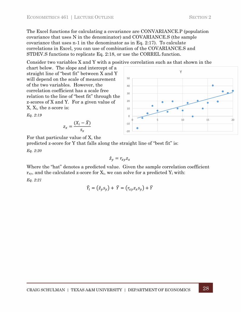
Consider two variables X and Y with a positive correlation such as that shown in the chart below. The slope and intercept of a straight line of “best fit” between X and Y will depend on the scale of measurement of the two variables. However, the correlation coefficient has a scale free relation to the line of “best fit” through the z-scores of X and Y. For a given value of X, Xi, the z-score is:
Eq. 2:19
For that particular value of X, the predicted z-score for Y that falls along the straight line of “best fit” is:
Eq. 2:20
Where the “hat” denotes a predicted value. Given the sample correlation coefficient rxy, and the calculated z-score for Xi, we can solve for a predicted Yi with:
Eq. 2:21
‐20
‐10
0
10
20
30
40
50
0 5 10 15 20
Y
SECTION 2 ECONOMETRICS 461 | LECTURE OUTLINE
CRAIG SCHULMAN | TEXAS A&M UNIVERSITY | DEPARTMENT OF ECONOMICS
29
E. Example Problems
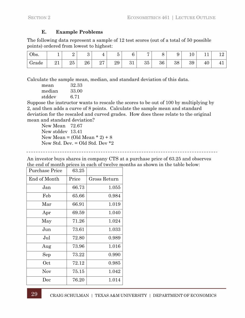
The following data represent a sample of 12 test scores (out of a total of 50 possible points) ordered from lowest to highest:
Obs. 1 2 3 4 5 6 7 8 9 10 11 12
Grade 21 25 26 27 29 31 35 36 38 39 40 41
Calculate the sample mean, median, and standard deviation of this data. mean 32.33 median 33.00 stddev 6.71
Suppose the instructor wants to rescale the scores to be out of 100 by multiplying by 2, and then adds a curve of 8 points. Calculate the sample mean and standard deviation for the rescaled and curved grades. How does these relate to the original mean and standard deviation?
New Mean 72.67 New stddev 13.41 New Mean = (Old Mean * 2) + 8 New Std. Dev. = Old Std. Dev *2
An investor buys shares in company CTS at a purchase price of 63.25 and observes the end of month prices in each of twelve months as shown in the table below: Purchase Price 63.25
End of Month Price Gross Return
Jan 66.73 1.055
Feb 65.66 0.984
Mar 66.91 1.019
Apr 69.59 1.040
May 71.26 1.024
Jun 73.61 1.033
Jul 72.80 0.989
Aug 73.96 1.016
Sep 73.22 0.990
Oct 72.12 0.985
Nov 75.15 1.042
Dec 76.20 1.014

ECONOMETRICS 461 | LECTURE OUTLINE SECTION 2
CRAIG SCHULMAN | TEXAS A&M UNIVERSITY | DEPARTMENT OF ECONOMICS
30
Calculate the geometric mean of the Gross Return data to get the Average Compound Monthly (Gross) Return.
√1.055 0.984 1.019 … 1.014 1.0156
OR
76.2063.25
1.0156
An investor purchases stock in two different companies, ABC and XYZ. Over a period of time, the following summary statistics of the two company’s stock prices are observed:
ABC XYZ
Mean Price 11.34 33.66
Std. Dev. Price 3.107 6.811
Covariance -16.129
Which of the two company’s stock prices exhibits more variability? Explain the basis for your answer.
Coefficient of Variation: ABC = 0.27 XYZ = 0.20 So ABC is more variable relative to the mean.
Calculate the correlation coefficient for the two company’s stock prices.
16.12911.34 33.66
0.762
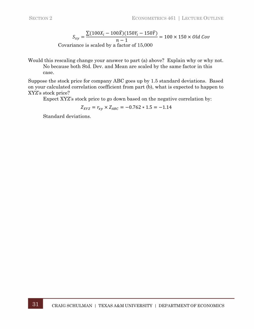
Suppose the stock prices are rescaled to account for number of shares purchased. ABC’s prices are rescaled by multiplying by 100 and XYZ’s prices are rescaled by multiplying by 150. What happens to the covariance of the stock prices from this rescaling?
SECTION 2 ECONOMETRICS 461 | LECTURE OUTLINE
CRAIG SCHULMAN | TEXAS A&M UNIVERSITY | DEPARTMENT OF ECONOMICS
31
∑ 100 100 150 1501
100 150
Covariance is scaled by a factor of 15,000
Would this rescaling change your answer to part (a) above? Explain why or why not. No because both Std. Dev. and Mean are scaled by the same factor in this case.
Suppose the stock price for company ABC goes up by 1.5 standard deviations. Based on your calculated correlation coefficient from part (b), what is expected to happen to XYZ’s stock price?
Expect XYZ’s stock price to go down based on the negative correlation by:
0.762 ∗ 1.5 1.14
Standard deviations.
ECONOMETRICS 461 | LECTURE OUTLINE SECTION 3
CRAIG SCHULMAN | TEXAS A&M UNIVERSITY | DEPARTMENT OF ECONOMICS
32
Section 3. PROBABILITY AND THE NORMAL PROBABILITY DISTRIBUTION
A. Probability and Probability Distribution Functions
The first two sections dealt with various measures of central tendency, variability, and co-movement. We now turn to the methods by which we can make statements in probability about random variables. A random variable X is a variable that takes on values out of a defined set of possibilities. We learned that a key measure of central tendency for X is the population mean, denoted µ. Our sample measure of the mean is the (arithmetic) mean, denoted . The key measures of variability were the population variance (σ2) and standard deviation (σ) with sample measures denoted as s2 and s. These measures give us an indication of how values of X may cluster around a particular point (the mean) and the degree to which values of X vary around that point (the standard deviation). What we need is a means of linking specific values of X to the probability of observing that value – this is the Probability Distribution Function or PDF, denoted f(X). The PDF maps specific values of the random variable X to the probability of that value being observed. Thus, for a specific value of X, say X0, the PDF f(X0) is such that
Eq. 3:1
By definition, all probabilities are bound on the interval [0, 1]. A probability of 1 means an event is certain to occur while a probability of zero means it is certain not to occur, and any value in between zero and one indicates the likelihood of observing a particular value. The probability function, f(X) is therefore also bound on the interval [0, 1].
The specific form of f(X) will depend on the nature of the random variable X. Random variables can be either discrete (X takes on a set of countable values, usually integers) or continuous (X can take on any value in an interval). Note that a discrete random variable could involve an infinite number of possibilities (any positive integer, for example) and that a continuous random variable could involve a very narrow range (any fractional value between 1 and 2, for example).
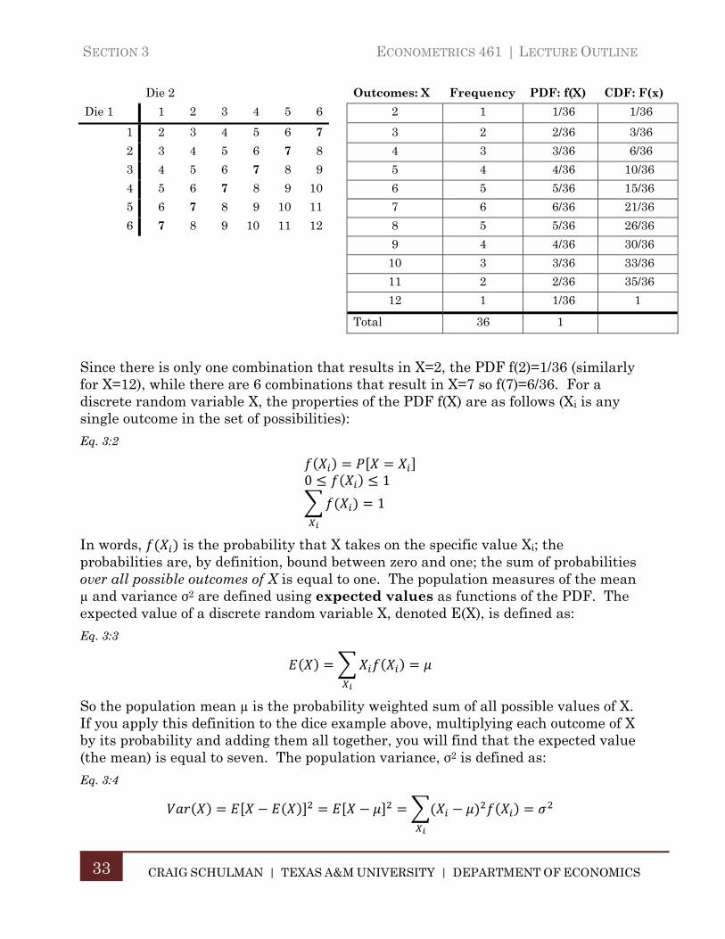
An example of a discrete random variable is the roll of a pair of six-sided dice with the faces numbered 1 to 6 and the outcome is the sum of the two die. As shown in the following table, there are 36 possible combinations of 11 discrete outcomes in the set {2, 3, 4, 5, 6, 7, 8, 9, 10, 11, 12}. Assuming the dice are “fair” so that the chances of any given number being rolled on one of the individual dies is equally likely, the probabilities of each outcome – the PDF, f(X) – is as shown in the following table:
SECTION 3 ECONOMETRICS 461 | LECTURE OUTLINE
CRAIG SCHULMAN | TEXAS A&M UNIVERSITY | DEPARTMENT OF ECONOMICS
33
Die 2 Outcomes: X Frequency PDF: f(X) CDF: F(x)
Die 1 1 2 3 4 5 6 2 1 1/36 1/36
1 2 3 4 5 6 7 3 2 2/36 3/36
2 3 4 5 6 7 8 4 3 3/36 6/36
3 4 5 6 7 8 9 5 4 4/36 10/36
4 5 6 7 8 9 10 6 5 5/36 15/36
5 6 7 8 9 10 11 7 6 6/36 21/36
6 7 8 9 10 11 12 8 5 5/36 26/36
9 4 4/36 30/36
10 3 3/36 33/36
11 2 2/36 35/36
12 1 1/36 1
Total 36 1
Since there is only one combination that results in X=2, the PDF f(2)=1/36 (similarly for X=12), while there are 6 combinations that result in X=7 so f(7)=6/36. For a discrete random variable X, the properties of the PDF f(X) are as follows (Xi is any single outcome in the set of possibilities):
Eq. 3:2
0 1
1
In words, is the probability that X takes on the specific value Xi; the probabilities are, by definition, bound between zero and one; the sum of probabilities over all possible outcomes of X is equal to one. The population measures of the mean µ and variance σ2 are defined using expected values as functions of the PDF. The expected value of a discrete random variable X, denoted E(X), is defined as:
Eq. 3:3
So the population mean µ is the probability weighted sum of all possible values of X. If you apply this definition to the dice example above, multiplying each outcome of X by its probability and adding them all together, you will find that the expected value (the mean) is equal to seven. The population variance, σ2 is defined as:
Eq. 3:4
ECONOMETRICS 461 | LECTURE OUTLINE SECTION 3
CRAIG SCHULMAN | TEXAS A&M UNIVERSITY | DEPARTMENT OF ECONOMICS
34
The standard deviation of X is simply the square root of the variance. While the PDF gives the probability that X will take on a particular value, the Cumulative Distribution Function, or CDF, is denoted F(X) and is the probability that X is less than or equal to a particular value. For a discrete random variable, the CDF has the following properties:
Eq. 3:5
0 1
Given the definition of the CDF and since the PDF must sum to 1, if we know the probability P[X ≤ Xi] = F(Xi) then P[X > Xi] = 1 – F(Xi). In the dice example above, for example, we know that the probability that X ≤ 5 from the CDF is 10/36 so the probability that X > 5 is 1 – 10/36 = 26/36. We can also use these properties to find the probability that X falls in a particular range. For example:
Eq. 3:6
For continuous random variables, the same basic properties of the PDF and CDF remain but the summations in the definitions above are replaced with integrals to measure the area under a continuous function. For example:
Eq. 3:7
The results related to rescaling a random variable by applying a linear function adding a constant a, and multiplying by a constant b that we covered previously, continue to hold in this context. For the random variable X and constants a and b, for example:
Eq. 3:8
B. Binomial Distribution
A Binomial random variable is one that can take on one of only two values: a “success” or a “failure.” The properties of such a random variable are as follows:
A fixed number of observations, n; for example, 13 tosses of a coin; 11 cell phones taken from a production line.
SECTION 3 ECONOMETRICS 461 | LECTURE OUTLINE
CRAIG SCHULMAN | TEXAS A&M UNIVERSITY | DEPARTMENT OF ECONOMICS
35
Two mutually exclusive and collectively exhaustive categories; “Heads” or “tails” on the toss of a coin; “Defective” or “not defective” for a given cell phone;
Constant probability of “success” for each observation;
Observations are independent: the outcome of one observation does not affect the outcome of another.
The form of the Binomial Distribution is derived from the number of possible successes that are possible in n independent experiments. The number of sequences with x successes in n independent experiments is given by:
Eq. 3:9
!! !
Where ! 1 2 … , 0! 1 Let P be the probability of a success for any single observation. Then Probability Distribution Function P(x) – the probability of x successes in n trials – for the Binomial Distribution is: Eq. 3:10
!! !
1
The Cumulative Distribution Function, F(x), is Eq. 3:11
!! !
1
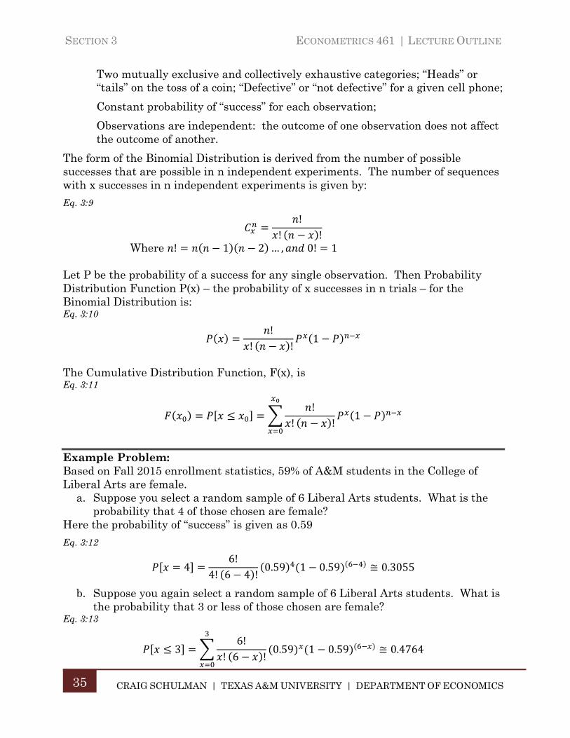
Example Problem: Based on Fall 2015 enrollment statistics, 59% of A&M students in the College of Liberal Arts are female.
a. Suppose you select a random sample of 6 Liberal Arts students. What is the probability that 4 of those chosen are female?
Here the probability of “success” is given as 0.59
Eq. 3:12
46!
4! 6 4 !0.59 1 0.59 ≅ 0.3055
b. Suppose you again select a random sample of 6 Liberal Arts students. What is the probability that 3 or less of those chosen are female?
Eq. 3:13
36!
! 6 !0.59 1 0.59 ≅ 0.4764
ECONOMETRICS 461 | LECTURE OUTLINE SECTION 3
CRAIG SCHULMAN | TEXAS A&M UNIVERSITY | DEPARTMENT OF ECONOMICS
36
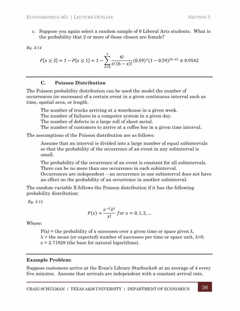
c. Suppose you again select a random sample of 6 Liberal Arts students. What is the probability that 2 or more of those chosen are female?
Eq. 3:14
2 1 1 16!
! 6 !0.59 1 0.59 ≅ 0.9542
C. Poisson Distribution
The Poisson probability distribution can be used the model the number of occurrences (or successes) of a certain event in a given continuous interval such as time, spatial area, or length.
The number of trucks arriving at a warehouse in a given week. The number of failures in a computer system in a given day. The number of defects in a large roll of sheet metal. The number of customers to arrive at a coffee bar in a given time interval.
The assumptions of the Poisson distribution are as follows:
Assume that an interval is divided into a large number of equal subintervals so that the probability of the occurrence of an event in any subinterval is small.
The probability of the occurrence of an event is constant for all subintervals. There can be no more than one occurrence in each subinterval. Occurrences are independent – an occurrence in one subinterval does not have an effect on the probability of an occurrence in another subinterval.
The random variable X follows the Poisson distribution if it has the following probability distribution:
Eq. 3:15
! 0, 1, 2, …
Where:
P(x) = the probability of x successes over a given time or space given λ. λ = the mean (or expected) number of successes per time or space unit, λ>0. e = 2.71828 (the base for natural logarithms).
Example Problem:
Suppose customers arrive at the Evan’s Library Starbucks® at an average of 4 every five minutes. Assume that arrivals are independent with a constant arrival rate,
SECTION 3 ECONOMETRICS 461 | LECTURE OUTLINE
CRAIG SCHULMAN | TEXAS A&M UNIVERSITY | DEPARTMENT OF ECONOMICS
37
and that arrivals follow the Poisson distribution, with X denoting the number of arrivals in a given five minute period and mean λ = 4.
a) Find the probability that 2 or fewer customers arrive in a five minute period.
The probability that X is 2 or less, P(X≤2) = P(X=0) + P(X=1) + P(X=2). With λ = 4, then
04
0!≅ 0.0183
14
1!≅ 0.0733
24
2!≅ 0.1465
So P(X≤2) = 0.0183 + 0.0733 + 0.1465 = 0.2381
b) Find the probability that more than 3 customers arrive in a five minute period.
The probability that X is more than 3, P(X>3) = 1 – P(X≤3). We found P(X≤2) in part a, above, and
34
3!≅ 0.1954
So P(X>3) = 1 – P(X≤3) = 1 – (0.0183 + 0.0733 + 0.1465 + 0.1954) = 0.5665
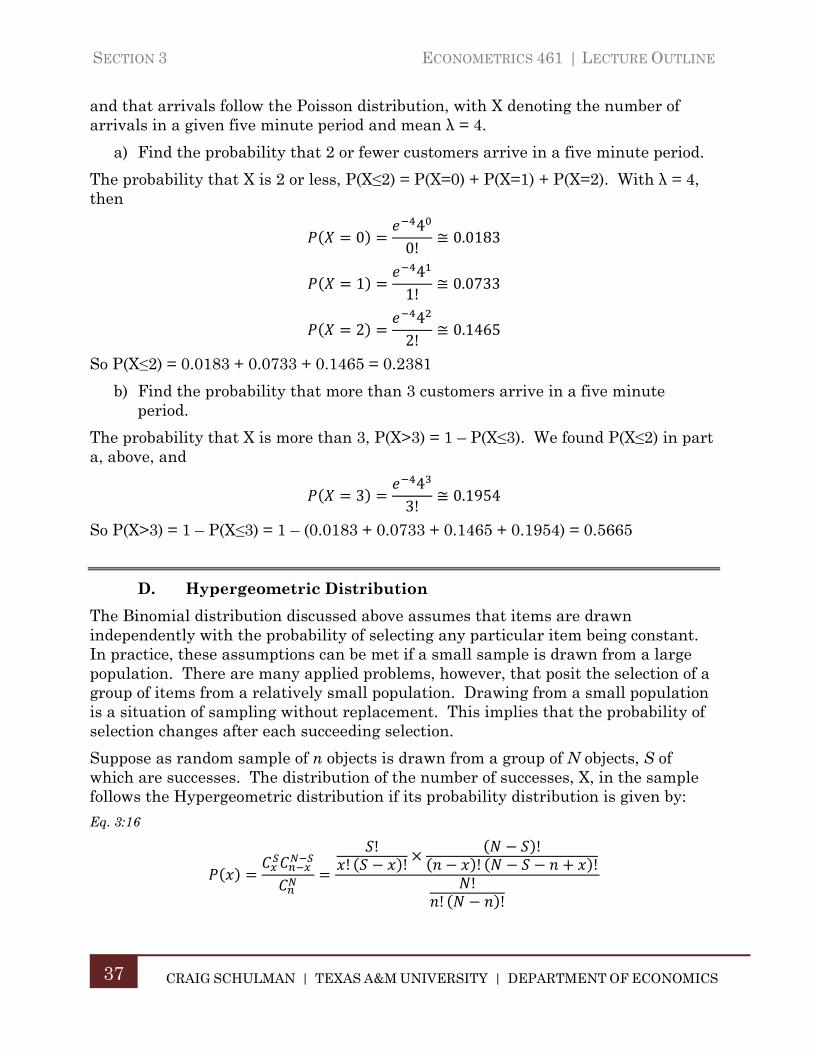
D. Hypergeometric Distribution
The Binomial distribution discussed above assumes that items are drawn independently with the probability of selecting any particular item being constant. In practice, these assumptions can be met if a small sample is drawn from a large population. There are many applied problems, however, that posit the selection of a group of items from a relatively small population. Drawing from a small population is a situation of sampling without replacement. This implies that the probability of selection changes after each succeeding selection.
Suppose as random sample of n objects is drawn from a group of N objects, S of which are successes. The distribution of the number of successes, X, in the sample follows the Hypergeometric distribution if its probability distribution is given by:
Eq. 3:16
!! !
!! !!
! !
ECONOMETRICS 461 | LECTURE OUTLINE SECTION 3
CRAIG SCHULMAN | TEXAS A&M UNIVERSITY | DEPARTMENT OF ECONOMICS
38
Where x can take on integer values from the larger of 0 and [n – (N – S)] and the smaller of n and S.
Example problem:
A financial analyst is given a list of 14 corporate bonds. Out of this list, 5 of the bonds would subsequently be downgraded. Suppose the analyst randomly selected 3 bonds from the list. What is the probability that at least 2 of the bonds chosen by the analyst were among those to be downgraded?
Here, the population size N=14, the number of success in the population S=4, and the sample size n=3. We want P(X≥2) = 1 – P(X≤1) = 1 – P(X=0) – P(X=1):
0
5!0! 5 0 !
14 5 !3 0 ! 14 5 3 0 !
14!3! 14 3 !
≅ 0.2308
1
5!1! 5 1 !
14 5 !3 1 ! 14 5 3 1 !
14!3! 14 3 !
≅ 0.4945
So, P(X≥2) = 1 – 0.2308 – 0.4945 = 0.2747
E. Exponential Distribution
The Binomial, Poisson, and Hypergeometric distributions are discrete distributions in that outcomes are countable (even though they by infinitely countable such as the number of grains of sand in a beach). The Exponential Distribution Function is a continuous distribution in that outcomes can take on any value greater than zero. It can be used to model the length of time between occurrences of an event.
Time between trucks arriving at a warehouse. Time between customers calling a help-line.
An Exponential random variable T (t>0) has a probability distribution function, f(t) as follows:
Eq. 3:17
Where:
λ is the mean number of occurrences per unit t (a time dimension or space dimension)
t is the number of units (time or space) e is the nature number = 2.71828 …
SECTION 3 ECONOMETRICS 461 | LECTURE OUTLINE
CRAIG SCHULMAN | TEXAS A&M UNIVERSITY | DEPARTMENT OF ECONOMICS
39
The mean number of units per occurrence is given by 1/λ
The Cumulative Distribution Function F(t) is given by:
Eq. 3:18
1 , 0
Example Problem:
For Cheryl’s Burger-Max restaurant, assume customer arrivals during the “lunch rush” follow the exponential distribution and that, on average, there are 45 customer arrivals per hour.
a) What is the probability that more than 2 minutes will elapse between customer arrivals?
Here λ=45 and t is measured in hours, so 2 minutes is (2/60) hours.
2 1 2 1 1 1 0.7779 0.2231
b) What is the probability that 3 minutes or less will elapse between customer arrivals?
3 1 0.8946
c) What is the probability that between 1.5 minutes and 2.5 minutes will elapse between customer arrivals?
2.5 1.5. .
0.1713
F. The Normal Distribution
The Normal Probability distribution is a symmetric bell-shaped distribution that is widely observed in nature and economics. A continuous random variable X with mean (expected value) µ and variance σ2 follows the normal probability distribution if the PDF of X has the following mathematical form:
Eq. 3:19
1
√2
And is denoted X~N(µ, σ2). Because of the mathematical form of the distribution, the integration required to derive the mean and variance cannot be directly solved, it must be computed numerically for different specific values of µ and σ2. However, because of the properties of linear functions of a random variable, any Normal random variable X can be standardized as its Z-score to get a Normal variable with a mean of zero and a standard deviation of 1. Thus, if X~N(µ, σ2), then:
ECONOMETRICS 461 | LECTURE OUTLINE SECTION 3
CRAIG SCHULMAN | TEXAS A&M UNIVERSITY | DEPARTMENT OF ECONOMICS
40
Eq. 3:20
~ 0, 1
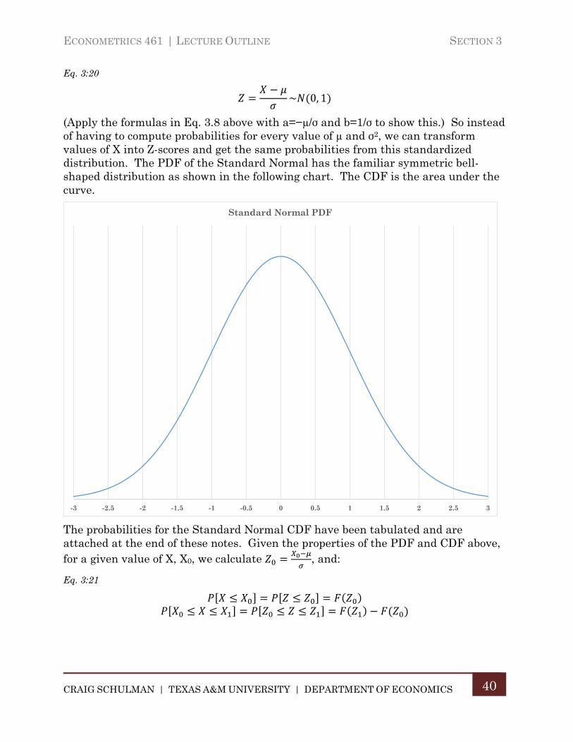
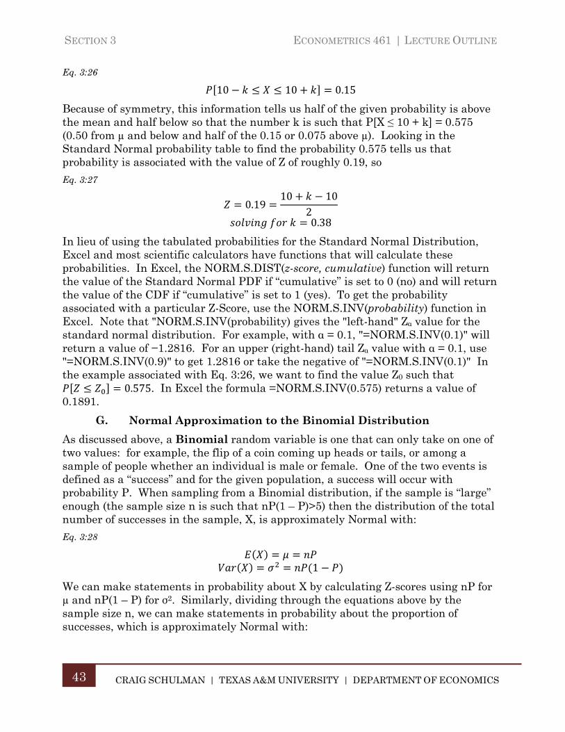
(Apply the formulas in Eq. 3.8 above with a=−µ/σ and b=1/σ to show this.) So instead of having to compute probabilities for every value of µ and σ2, we can transform values of X into Z-scores and get the same probabilities from this standardized distribution. The PDF of the Standard Normal has the familiar symmetric bell-shaped distribution as shown in the following chart. The CDF is the area under the curve.
The probabilities for the Standard Normal CDF have been tabulated and are attached at the end of these notes. Given the properties of the PDF and CDF above, for a given value of X, X0, we calculate , and:
Eq. 3:21
-3 -2.5 -2 -1.5 -1 -0.5 0 0.5 1 1.5 2 2.5 3
Standard Normal PDF
SECTION 3 ECONOMETRICS 461 | LECTURE OUTLINE
CRAIG SCHULMAN | TEXAS A&M UNIVERSITY | DEPARTMENT OF ECONOMICS
41
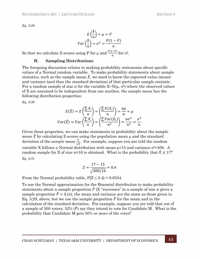
‐3 ‐2.5 ‐2 ‐1.5 ‐1 ‐0.5 0 0.5 1 1.5 2 2.5 3
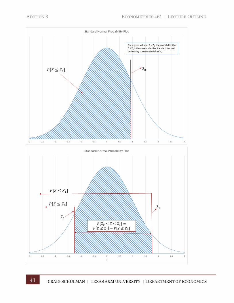
Standard Normal Probability Plot
For a given value of Z = Z0, the probability that Z ≤ Z0 is the area under the Standard Normal probability curve to the left of Z0
Z0
‐3 ‐2.5 ‐2 ‐1.5 ‐1 ‐0.5 0 0.5 1 1.5 2 2.5 3
Z
Standard Normal Probability Plot
Z1
Z0
ECONOMETRICS 461 | LECTURE OUTLINE SECTION 3
CRAIG SCHULMAN | TEXAS A&M UNIVERSITY | DEPARTMENT OF ECONOMICS
42
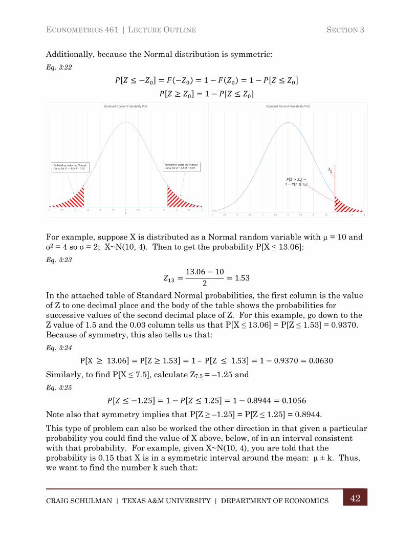
Additionally, because the Normal distribution is symmetric:
Eq. 3:22
1 1
1
For example, suppose X is distributed as a Normal random variable with µ = 10 and σ2 = 4 so σ = 2; X~N(10, 4). Then to get the probability P[X ≤ 13.06]:
Eq. 3:23
13.06 102
1.53
In the attached table of Standard Normal probabilities, the first column is the value of Z to one decimal place and the body of the table shows the probabilities for successive values of the second decimal place of Z. For this example, go down to the Z value of 1.5 and the 0.03 column tells us that P[X ≤ 13.06] = P[Z ≤ 1.53] = 0.9370. Because of symmetry, this also tells us that:
Eq. 3:24
P X 13.06 P Z 1.53 1– P Z 1.53 1 0.9370 0.0630
Similarly, to find P[X ≤ 7.5], calculate Z7.5 = –1.25 and
Eq. 3:25
1.25 1 1.25 1 0.8944 0.1056
Note also that symmetry implies that P[Z ≥ –1.25] = P[Z ≤ 1.25] = 0.8944.
This type of problem can also be worked the other direction in that given a particular probability you could find the value of X above, below, of in an interval consistent with that probability. For example, given X~N(10, 4), you are told that the probability is 0.15 that X is in a symmetric interval around the mean: µ ± k. Thus, we want to find the number k such that:
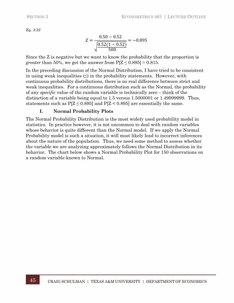
‐3 ‐2.5 ‐2 ‐1.5 ‐1 ‐0.5 0 0.5 1 1.5 2 2.5 3
Standard Normal Probability Plot
Z0
‐3 ‐2.5 ‐2 ‐1.5 ‐1 ‐0.5 0 0.5 1 1.5 2 2.5 3
Z
Standard Normal Probability Plot
Probability under the Normal Curve for Z > 1.645 = 0.05
Probability under the Normal Curve for Z < -1.645 = 0.05
SECTION 3 ECONOMETRICS 461 | LECTURE OUTLINE
CRAIG SCHULMAN | TEXAS A&M UNIVERSITY | DEPARTMENT OF ECONOMICS
43
Eq. 3:26
10 10 0.15
Because of symmetry, this information tells us half of the given probability is above the mean and half below so that the number k is such that P[X ≤ 10 + k] = 0.575 (0.50 from µ and below and half of the 0.15 or 0.075 above µ). Looking in the Standard Normal probability table to find the probability 0.575 tells us that probability is associated with the value of Z of roughly 0.19, so
Eq. 3:27
0.1910 10
2
0.38
In lieu of using the tabulated probabilities for the Standard Normal Distribution, Excel and most scientific calculators have functions that will calculate these probabilities. In Excel, the NORM.S.DIST(z-score, cumulative) function will return the value of the Standard Normal PDF if “cumulative” is set to 0 (no) and will return the value of the CDF if “cumulative” is set to 1 (yes). To get the probability associated with a particular Z-Score, use the NORM.S.INV(probability) function in Excel. Note that "NORM.S.INV(probability) gives the "left-hand" Zα value for the standard normal distribution. For example, with α = 0.1, "=NORM.S.INV(0.1)" will return a value of −1.2816. For an upper (right-hand) tail Zα value with α = 0.1, use "=NORM.S.INV(0.9)" to get 1.2816 or take the negative of "=NORM.S.INV(0.1)" In the example associated with Eq. 3:26, we want to find the value Z0 such that
0.575. In Excel the formula =NORM.S.INV(0.575) returns a value of 0.1891.
G. Normal Approximation to the Binomial Distribution
As discussed above, a Binomial random variable is one that can only take on one of two values: for example, the flip of a coin coming up heads or tails, or among a sample of people whether an individual is male or female. One of the two events is defined as a “success” and for the given population, a success will occur with probability P. When sampling from a Binomial distribution, if the sample is “large” enough (the sample size n is such that nP(1 – P)>5) then the distribution of the total number of successes in the sample, X, is approximately Normal with:
Eq. 3:28
1
We can make statements in probability about X by calculating Z-scores using nP for µ and nP(1 – P) for σ2. Similarly, dividing through the equations above by the sample size n, we can make statements in probability about the proportion of successes, which is approximately Normal with:
ECONOMETRICS 461 | LECTURE OUTLINE SECTION 3
CRAIG SCHULMAN | TEXAS A&M UNIVERSITY | DEPARTMENT OF ECONOMICS
44
Eq. 3:29
1
So that we calculate Z-scores using P for µ and for σ2.
H. Sampling Distributions
The foregoing discussion relates to making probability statements about specific values of a Normal random variable. To make probability statements about sample statistics, such as the sample mean , we need to know the expected value (mean) and variance (and thus the standard deviation) of that particular sample statistic. For a random sample of size n for the variable X~N(µ, σ2) where the observed values of X are assumed to be independent from one another, the sample mean has the following distribution properties:
Eq. 3:30
∑ ∑
∑ ∑
Given these properties, we can make statements in probability about the sample mean by calculating Z-scores using the population mean µ and the standard deviation of the sample mean
√. For example, suppose you are told the random
variable X follows a Normal distribution with mean µ=15 and variance σ2=400. A random sample for X of size n=16 is obtained. What is the probability that 17?
Eq. 3:31
17 15
400/160.4
From the Normal probability table, P[Z ≤ 0.4] = 0.6554.
To use the Normal approximation for the Binomial distribution to make probability statements about a sample proportion (X “successes” in a sample of size n gives a sample proportion / ), the mean and variance are the same as those given in Eq. 3:29, above, but we use the sample proportion for the mean and in the calculation of the standard deviation. For example, suppose you are told that out of a sample of 500 voters, 52% ( ) say they intend to vote for Candidate M. What is the probability that Candidate M gets 50% or more of the votes?
SECTION 3 ECONOMETRICS 461 | LECTURE OUTLINE
CRAIG SCHULMAN | TEXAS A&M UNIVERSITY | DEPARTMENT OF ECONOMICS
45
Eq. 3:32
0.50 0.52
0.52 1 0.52500
0.895
Since the Z is negative but we want to know the probability that the proportion is greater than 50%, we get the answer from P[Z ≤ 0.895] ≈ 0.815.
In the preceding discussion of the Normal Distribution, I have tried to be consistent in using weak inequalities (≤) in the probability statements. However, with continuous probability distributions, there is no real difference between strict and weak inequalities. For a continuous distribution such as the Normal, the probability of any specific value of the random variable is technically zero – think of the distinction of a variable being equal to 1.5 versus 1.5000001 or 1.49999999. Thus, statements such as P[Z ≤ 0.895] and P[Z < 0.895] are essentially the same.
I. Normal Probability Plots
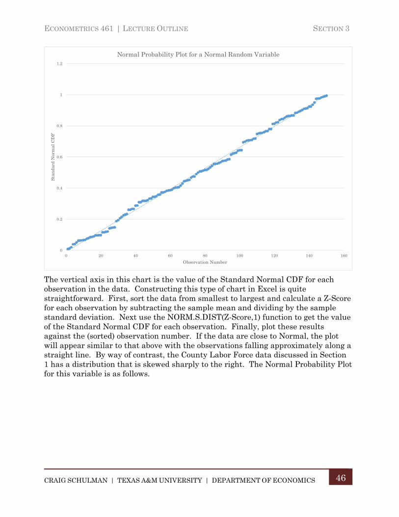
The Normal Probability Distribution is the most widely used probability model in statistics. In practice however, it is not uncommon to deal with random variables whose behavior is quite different than the Normal model. If we apply the Normal Probability model is such a situation, it will most likely lead to incorrect inferences about the nature of the population. Thus, we need some method to assess whether the variable we are analyzing approximately follows the Normal Distribution in its behavior. The chart below shows a Normal Probability Plot for 150 observations on a random variable known to Normal.
ECONOMETRICS 461 | LECTURE OUTLINE SECTION 3
CRAIG SCHULMAN | TEXAS A&M UNIVERSITY | DEPARTMENT OF ECONOMICS
46
The vertical axis in this chart is the value of the Standard Normal CDF for each observation in the data. Constructing this type of chart in Excel is quite straightforward. First, sort the data from smallest to largest and calculate a Z-Score for each observation by subtracting the sample mean and dividing by the sample standard deviation. Next use the NORM.S.DIST(Z-Score,1) function to get the value of the Standard Normal CDF for each observation. Finally, plot these results against the (sorted) observation number. If the data are close to Normal, the plot will appear similar to that above with the observations falling approximately along a straight line. By way of contrast, the County Labor Force data discussed in Section 1 has a distribution that is skewed sharply to the right. The Normal Probability Plot for this variable is as follows.
0
0.2
0.4
0.6
0.8
1
1.2
0 20 40 60 80 100 120 140 160
Sta
nda
rd N
orm
al C
DF
Observation Number
Normal Probability Plot for a Normal Random Variable
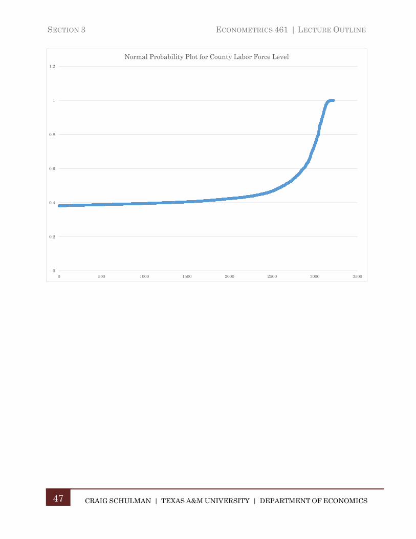
SECTION 3 ECONOMETRICS 461 | LECTURE OUTLINE
CRAIG SCHULMAN | TEXAS A&M UNIVERSITY | DEPARTMENT OF ECONOMICS
47
0
0.2
0.4
0.6
0.8
1
1.2
0 500 1000 1500 2000 2500 3000 3500
Normal Probability Plot for County Labor Force Level
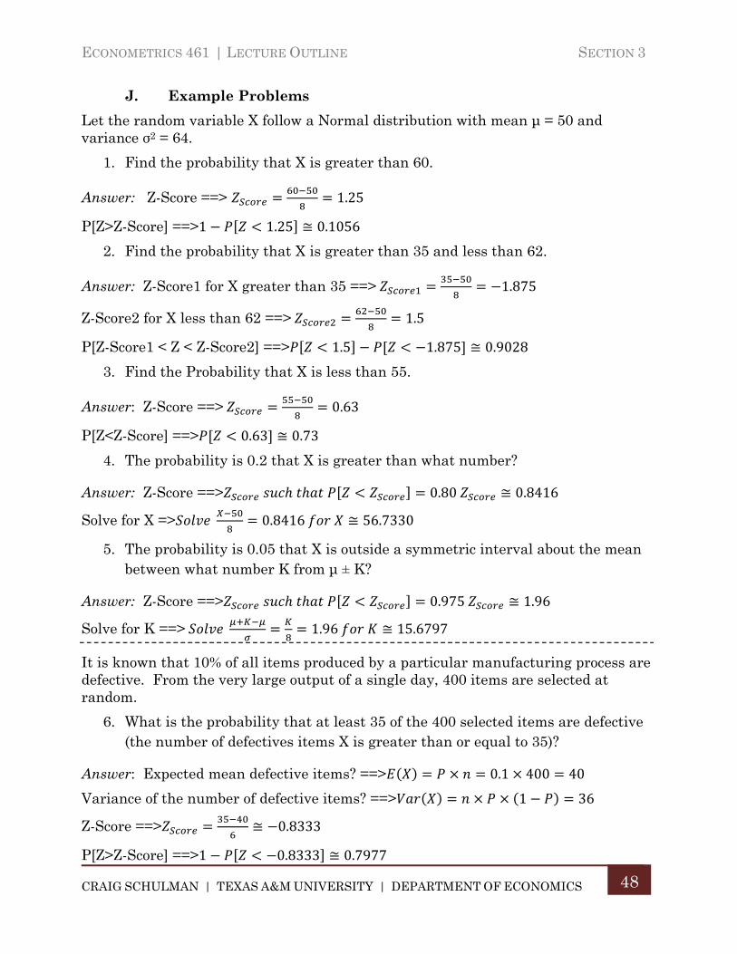
ECONOMETRICS 461 | LECTURE OUTLINE SECTION 3
CRAIG SCHULMAN | TEXAS A&M UNIVERSITY | DEPARTMENT OF ECONOMICS
48
J. Example Problems
Let the random variable X follow a Normal distribution with mean μ = 50 and variance σ2 = 64.
1. Find the probability that X is greater than 60.
Answer: Z-Score ==> 1.25
P[Z>Z-Score] ==>1 1.25 ≅ 0.1056
2. Find the probability that X is greater than 35 and less than 62.
Answer: Z-Score1 for X greater than 35 ==> 1.875
Z-Score2 for X less than 62 ==> 1.5
P[Z-Score1 < Z < Z-Score2] ==> 1.5 1.875 ≅ 0.9028
3. Find the Probability that X is less than 55.
Answer: Z-Score ==> 0.63
P[Z<Z-Score] ==> 0.63 ≅ 0.73
4. The probability is 0.2 that X is greater than what number?
Answer: Z-Score ==> 0.80 ≅ 0.8416
Solve for X => 0.8416 ≅ 56.7330
5. The probability is 0.05 that X is outside a symmetric interval about the mean between what number K from μ ± K?
Answer: Z-Score ==> 0.975 ≅ 1.96
Solve for K ==> 1.96 ≅ 15.6797
It is known that 10% of all items produced by a particular manufacturing process are defective. From the very large output of a single day, 400 items are selected at random.
6. What is the probability that at least 35 of the 400 selected items are defective (the number of defectives items X is greater than or equal to 35)?
Answer: Expected mean defective items? ==> 0.1 400 40
Variance of the number of defective items? ==> 1 36
Z-Score ==> ≅ 0.8333
P[Z>Z-Score] ==>1 0.8333 ≅ 0.7977
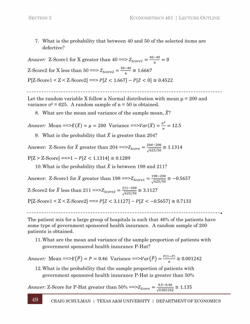
SECTION 3 ECONOMETRICS 461 | LECTURE OUTLINE
CRAIG SCHULMAN | TEXAS A&M UNIVERSITY | DEPARTMENT OF ECONOMICS
49
7. What is the probability that between 40 and 50 of the selected items are defective?
Answer: Z-Score1 for X greater than 40 ==> 0
Z-Score2 for X less than 50 ==> ≅ 1.6667
P[Z-Score1 < Z < Z-Score2] ==> 1.667 0 ≅ 0.4522
Let the random variable X follow a Normal distribution with mean μ = 200 and variance σ2 = 625. A random sample of n = 50 is obtained.
8. What are the mean and variance of the sample mean, ?
Answer: Mean ==> 200 Variance ==> 12.5
9. What is the probability that is greater than 204?
Answer: Z-Score for greater than 204 ==>/
≅ 1.1314
P[Z > Z-Score] ==>1 1.1314 ≅ 0.1289
10. What is the probability that is between 198 and 211?
Answer: Z-Score1 for greater than 198 ==>/
≅ 0.5657
Z-Score2 for less than 211 ==>/
≅ 3.1127
P[Z-Score1 < Z < Z-Score2] ==> 3.1127 0.5657 ≅ 0.7133
The patient mix for a large group of hospitals is such that 46% of the patients have some type of government sponsored health insurance. A random sample of 200 patients is obtained.
11. What are the mean and variance of the sample proportion of patients with government sponsored health insurance P-Hat?
Answer: Mean ==> 0.46 Variance ==> ≅ 0.001242
12. What is the probability that the sample proportion of patients with government sponsored health insurance P-Hat is greater than 50%
Answer: Z-Score for P-Hat greater than 50% ==> . .
√ .≅ 1.135
ECONOMETRICS 461 | LECTURE OUTLINE SECTION 3
CRAIG SCHULMAN | TEXAS A&M UNIVERSITY | DEPARTMENT OF ECONOMICS
50
P[Z > Z-Score] ==>1 1.135 ≅ 0.1282
13. What is the probability that the sample proportion of patients with government sponsored health insurance P-Hat is between 42% and 48%?
Answer: Z-Score1 for P-Hat greater than 42% ==> . .
√ .≅ 1.135
Z-Score2 for p-Hat less than 48%==> . .
√ .≅ 0.5675
P[Z-Score1 < Z < Z-Score2] ==> 0.5675 1.135 ≅ 0.5866
SECTION 4 ECONOMETRICS 461 | LECTURE OUTLINE
CRAIG SCHULMAN | TEXAS A&M UNIVERSITY | DEPARTMENT OF ECONOMICS
51
Section 4. ESTIMATION AND HYPOTHESIS TESTING
A. Sampling Distributions
We introduced the notion of Sampling Distributions in Section 3, above, but the topic bears repeating. Given a random sample of a random variable X that has a constant mean µ and constant variance σ2 (denoted X~(µ, σ2)) the Sampling Distribution is the PDF of the various sample statistics such as the sample mean, sample variance, and sample proportion. Given the random variable X~(µ, σ2), the sample mean has the following distribution properties:
Eq. 4:1
∑
/ /√~ 0, 1
The Central Limit Theorem states that for a random variable X~(µ, σ2), as the sample size n becomes “large” then Z as defined above is approximately Normally distributed. Thus, for any random variable with a constant mean and variance, we can make statements in probability about the sample mean based on the Normal probability distribution when we have a sufficiently large sample (usually, 20 or more observations is a sufficiently large sample).
If X is a binomial random variable that takes on a value of one (a “success”) with probability P and is zero with probability (1 – P), the sample proportion ∑ / has the following distribution properties:
Eq. 4:2
1
1 /~ 0, 1 " "
To get the sampling distribution of the sample variance S2, we need to introduce a probability distribution related to the Normal. If Z~N(0, 1) then Z2 is distributed as a Chi-Squared random variable with 1 degree of freedom. This is denoted . If Z1, Z2, …, Zn are independently distributed N(0, 1) then ∑ ~ (Chi-Squared with n degrees of freedom). The sample variance then has the following distribution properties:
ECONOMETRICS 461 | LECTURE OUTLINE SECTION 4
CRAIG SCHULMAN | TEXAS A&M UNIVERSITY | DEPARTMENT OF ECONOMICS
52
Eq. 4:3
1
~
The Chi-Square distribution is not symmetric so you must be careful to identify whether you are looking at lower tail versus upper tail probabilities. A copy of the Chi-Square probability tables are attached at the end of these notes. In Excel, the CHISQ.DIST(stat, degrees-of-freedom, cumulative) returns the “left tail” probability (the probability of finding a value less than “stat”) under the Chi-Square distribution if cumulative is set to yes (1). CHISQ.DIST.RT returns the “right tail” probability.
B. Confidence Intervals: Single Sample
The forgoing distribution properties allow us to make probability statements about the various sample statistics similar to those we constructed for Normal random variables. In particular, we can construct Confidence Intervals for the various sample statistics. For the random variable X~(µ,σ2) where the population variance σ2 is known, given a sufficiently large sample of size n, we can construct the Z-score for the sample mean:
Eq. 4:4
/√~ 0, 1
Now if we choose a Confidence Level, (1 – α) where α is the chosen significance level between zero and one: for example, for a 90% confidence level, α=0.1 or 10%. Next, split α in half so that there is a probability of α/2 in each tail of the Normal distribution. Finding the Z value associated with α/2 then allows us to set up the following:
Eq. 4:5
1
√
1
Rearranging the terms inside the brackets, we can say that there is a probability of (1 – α) that the population mean µ is in the interval:
Eq. 4:6
√ √,
:√
,
:√
,
SECTION 4 ECONOMETRICS 461 | LECTURE OUTLINE
CRAIG SCHULMAN | TEXAS A&M UNIVERSITY | DEPARTMENT OF ECONOMICS
53
:√
,
:√
For example, suppose the random variable X has a known variance σ2=144. With a random sample of 25 observations, if we wanted to construct of 90% confidence interval, we need to find the value of Z such there is 5% in the upper right tail:
0.05, or 1 0.95. From the Normal probability table Zα/2 ≈
1.645. Because of symmetry of the Normal this also tells us that 0.05.
Therefore, there is a 90% probability that the population mean is in the interval:
Eq. 4:7
12
√251.645
2.4 1.645 3.948
If the population variance for our random variable X is unknown, we need to use yet another distribution related to the Normal: the t-distribution. The t-distribution is a ratio of a Standard Normal random variable and the square root of a Chi-Square random variable and makes use of the sampling distribution of the sample variance in Eq. 4:3 above. Like the Normal distribution, the t-distribution is symmetric and gets closer and closer to the Normal as the sample size increases. Replacing the population standard deviation σ in our Z-score with the sample standard deviation S, we get the tStat:
Eq. 4:8
/√~
A t-distribution with (n-1) degrees of freedom. The interval for a (1 – α)% confidence level is then given by:
Eq. 4:9
√, /
Thus, we replace the population standard deviation with the sample standard deviation and use values out of the table of probabilities for the t-distribution rather than the standard Normal distribution. A copy of the probability tables for the t-distribution is attached at the end of these notes.
For the sample proportion from a binomial random variable (see Eq. 4:2, above) if the sample size n is “large” ( 1 5 then the (1 – α)% confidence interval is calculated from:
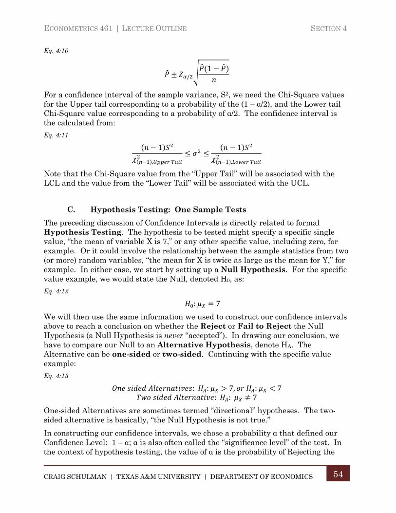
ECONOMETRICS 461 | LECTURE OUTLINE SECTION 4
CRAIG SCHULMAN | TEXAS A&M UNIVERSITY | DEPARTMENT OF ECONOMICS
54
Eq. 4:10
/1
For a confidence interval of the sample variance, S2, we need the Chi-Square values for the Upper tail corresponding to a probability of the (1 – α/2), and the Lower tail Chi-Square value corresponding to a probability of α/2. The confidence interval is the calculated from:
Eq. 4:11
1
,
1
,
Note that the Chi-Square value from the “Upper Tail” will be associated with the LCL and the value from the “Lower Tail” will be associated with the UCL.
C. Hypothesis Testing: One Sample Tests
The preceding discussion of Confidence Intervals is directly related to formal Hypothesis Testing. The hypothesis to be tested might specify a specific single value, “the mean of variable X is 7,” or any other specific value, including zero, for example. Or it could involve the relationship between the sample statistics from two (or more) random variables, “the mean for X is twice as large as the mean for Y,” for example. In either case, we start by setting up a Null Hypothesis. For the specific value example, we would state the Null, denoted H0, as:
Eq. 4:12
: 7
We will then use the same information we used to construct our confidence intervals above to reach a conclusion on whether the Reject or Fail to Reject the Null Hypothesis (a Null Hypothesis is never “accepted”). In drawing our conclusion, we have to compare our Null to an Alternative Hypothesis, denote HA. The Alternative can be one-sided or two-sided. Continuing with the specific value example:
Eq. 4:13
: : 7, : 7 : : 7
One-sided Alternatives are sometimes termed “directional” hypotheses. The two-sided alternative is basically, “the Null Hypothesis is not true.”
In constructing our confidence intervals, we chose a probability α that defined our Confidence Level: 1 – α; α is also often called the “significance level” of the test. In the context of hypothesis testing, the value of α is the probability of Rejecting the
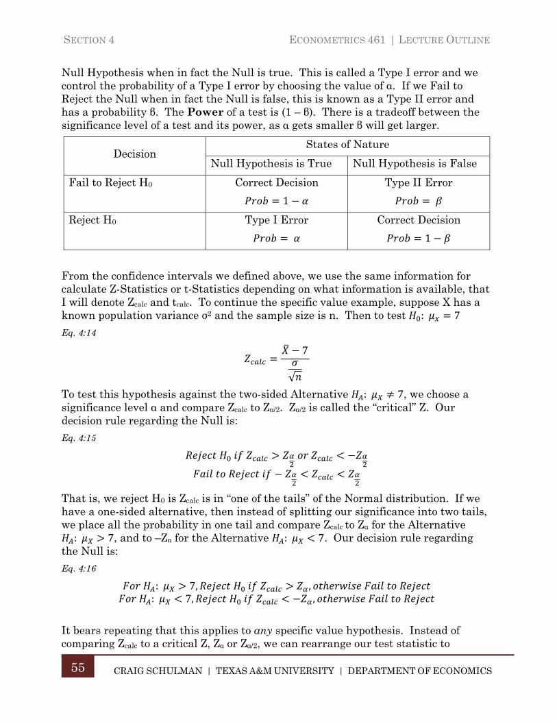
SECTION 4 ECONOMETRICS 461 | LECTURE OUTLINE
CRAIG SCHULMAN | TEXAS A&M UNIVERSITY | DEPARTMENT OF ECONOMICS
55
Null Hypothesis when in fact the Null is true. This is called a Type I error and we control the probability of a Type I error by choosing the value of α. If we Fail to Reject the Null when in fact the Null is false, this is known as a Type II error and has a probability β. The Power of a test is (1 – β). There is a tradeoff between the significance level of a test and its power, as α gets smaller β will get larger.
Decision States of Nature
Null Hypothesis is True Null Hypothesis is False
Fail to Reject H0 Correct Decision
1
Type II Error
Reject H0 Type I Error
Correct Decision
1
From the confidence intervals we defined above, we use the same information for calculate Z-Statistics or t-Statistics depending on what information is available, that I will denote Zcalc and tcalc. To continue the specific value example, suppose X has a known population variance σ2 and the sample size is n. Then to test : 7
Eq. 4:14
7
√
To test this hypothesis against the two-sided Alternative : 7, we choose a significance level α and compare Zcalc to Zα/2. Zα/2 is called the “critical” Z. Our decision rule regarding the Null is:
Eq. 4:15
That is, we reject H0 is Zcalc is in “one of the tails” of the Normal distribution. If we have a one-sided alternative, then instead of splitting our significance into two tails, we place all the probability in one tail and compare Zcalc to Zα for the Alternative : 7, and to –Zα for the Alternative : 7. Our decision rule regarding
the Null is:
Eq. 4:16
: 7, , : 7, ,
It bears repeating that this applies to any specific value hypothesis. Instead of comparing Zcalc to a critical Z, Zα or Zα/2, we can rearrange our test statistic to
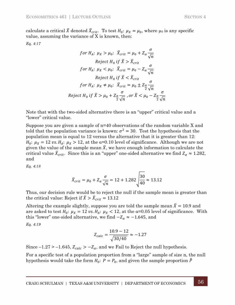
ECONOMETRICS 461 | LECTURE OUTLINE SECTION 4
CRAIG SCHULMAN | TEXAS A&M UNIVERSITY | DEPARTMENT OF ECONOMICS
56
calculate a critical denoted . To test : , where µ0 is any specific value, assuming the variance of X is known, then:
Eq. 4:17
: :√
: :√
: :√
√
, √
Note that with the two-sided alternative there is an “upper” critical value and a “lower” critical value.
Suppose you are given a sample of n=40 observations of the random variable X and told that the population variance is known: 30. Test the hypothesis that the population mean is equal to 12 versus the alternative that it is greater than 12: : 12 . : 12, at the α=0.10 level of significance. Although we are not
given the value of the sample mean , we have enough information to calculate the critical value . Since this is an “upper” one-sided alternative we find 1.282, and
Eq. 4:18
√12 1.282
3040
13.12
Thus, our decision rule would be to reject the null if the sample mean is greater than the critical value: Reject if 13.12
Altering the example slightly, suppose you are told the sample mean 10.9 and are asked to test : 12 . : 12, at the α=0.05 level of significance. With this “lower” one-sided alternative, we find 1.645, and
Eq. 4:19
10.9 12
30/401.27
Since –1.27 > –1.645, , and we Fail to Reject the null hypothesis.
For a specific test of a population proportion from a “large” sample of size n, the null hypothesis would take the form : , and given the sample proportion
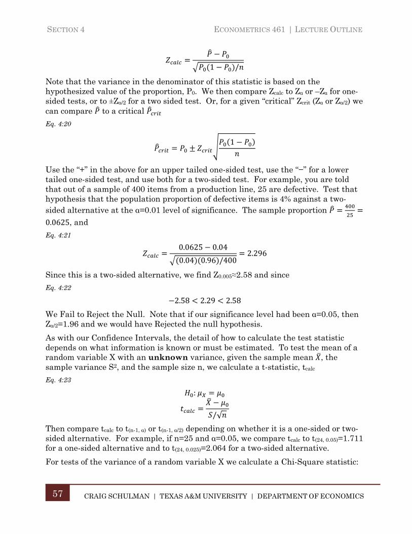
SECTION 4 ECONOMETRICS 461 | LECTURE OUTLINE
CRAIG SCHULMAN | TEXAS A&M UNIVERSITY | DEPARTMENT OF ECONOMICS
57
1 /
Note that the variance in the denominator of this statistic is based on the hypothesized value of the proportion, P0. We then compare Zcalc to Zα or –Zα for one-sided tests, or to ±Zα/2 for a two sided test. Or, for a given “critical” Zcrit (Zα or Zα/2) we can compare to a critical
Eq. 4:20
1
Use the “+” in the above for an upper tailed one-sided test, use the “−” for a lower tailed one-sided test, and use both for a two-sided test. For example, you are told that out of a sample of 400 items from a production line, 25 are defective. Test that hypothesis that the population proportion of defective items is 4% against a two-sided alternative at the α=0.01 level of significance. The sample proportion
0.0625, and
Eq. 4:21
0.0625 0.04
0.04 0.96 /4002.296
Since this is a two-sided alternative, we find Z0.005≈2.58 and since
Eq. 4:22
2.58 2.29 2.58
We Fail to Reject the Null. Note that if our significance level had been α=0.05, then Zα/2=1.96 and we would have Rejected the null hypothesis.
As with our Confidence Intervals, the detail of how to calculate the test statistic depends on what information is known or must be estimated. To test the mean of a random variable X with an unknown variance, given the sample mean , the sample variance S2, and the sample size n, we calculate a t-statistic, tcalc
Eq. 4:23
:
/√
Then compare tcalc to t(n-1, α) or t(n-1, α/2) depending on whether it is a one-sided or two-sided alternative. For example, if n=25 and α=0.05, we compare tcalc to t(24, 0.05)=1.711 for a one-sided alternative and to t(24, 0.025)=2.064 for a two-sided alternative.
For tests of the variance of a random variable X we calculate a Chi-Square statistic:
ECONOMETRICS 461 | LECTURE OUTLINE SECTION 4
CRAIG SCHULMAN | TEXAS A&M UNIVERSITY | DEPARTMENT OF ECONOMICS
58
Eq. 4:24
: 1
, ,
D. Confidence Intervals: Two Sample
We now turn to intervals for the difference between the sample statistics for two random variables. Suppose you have a random variable X with mean and variance : ~ , ; and the random variable Y with mean and variance : ~ , . The nature of the sampling distributions for the difference between the
sample statistics of these two random variables will depend on whether the samples are dependent or independent.
Dependent Samples
A dependent sample is such that each specific observation in the sample for X can be linked with a specific observation in the sample for Y. Consider the following example. A sample of n students is given an aptitude test and the scores are recorded. Call this initial set of scores the random variable X. The same set of students then participate in a test preparation course, after which they retake the aptitude test. Call the recorded set of scores for this second round of testing the random variable Y. The score for each specific student in the first round of testing, Xi, can be linked to that student’s score on the second round of testing, Yi. Define the difference between the two test scores as: . In this example, I have defined the difference as “before” minus “after” but it can be defined the other way as well. The difference variable di has the following properties:
Eq. 4:25
∑ ∑
∑
1
12
Given the sample mean of the difference variable, and its sample variance , and assuming the sample size is large enough to apply the Central Limit Theorem, the (1 – α)% confidence interval with significance for the difference in the population means is given by:
Eq. 4:26
√ ,
√ ,
SECTION 4 ECONOMETRICS 461 | LECTURE OUTLINE
CRAIG SCHULMAN | TEXAS A&M UNIVERSITY | DEPARTMENT OF ECONOMICS
59
√ ,
:√ ,
Note that the interval is calculated using the sample standard deviation of the difference variable and uses the t-distribution with degrees of freedom based on the number of pairs of observations, n – 1.
Independent Samples
Suppose we have two random variables X and Y with means and variances as defined in (1) above. Now, however, suppose that the samples for X and Y are independent of one another. To continue with a modified version of the testing example above, suppose a sample of students who are Economics majors are administered the aptitude test and scores are recorded as the random variable X. A second sample of students who are Sociology majors are also administered the test and their scores recorded as the random variable Y. If the population variances of the two variables are known, then the difference in the sample means, , has the following properties:
Eq. 4:27
And the (1 – α)% confidence interval for the difference in the population means is given by:
Eq. 4:28
Now suppose that the population variances for our two independent samples are unknown but assumed to be equal, so: . The variance of the difference in the sample means is now:
Eq. 4:29
1 1
ECONOMETRICS 461 | LECTURE OUTLINE SECTION 4
CRAIG SCHULMAN | TEXAS A&M UNIVERSITY | DEPARTMENT OF ECONOMICS
60
Since the (assumed equal) population variance σ2 is unknown, we need a sample estimate. Given the sample variance for X and Y, and , as an estimate of the (assumed equal) variance σ2 we calculate a pooled sample variance as:
Eq. 4:30
1 12
And the (1 – α)% confidence interval for the difference in the population means is given by:
Eq. 4:31
,
So we use a pooled estimate of the population variance and the t-distribution with degrees of freedom based on the sum of the sample sizes: 2 .
Now suppose that the population variances for our two independent samples are unknown but not assumed to be equal. The variance of the difference in the sample means is now:
Eq. 4:32
Given the sample variances for X and Y, and , the (1 – α)% confidence interval for the difference in the population means is similar to that in (9) above, but the extra uncertainty introduced by the unequal variances requires a complicated adjustment to the degrees of freedom for the t-distribution.
Eq. 4:33
,
Where the degrees of freedom, m is calculated from:
Eq. 4:34
1 1
SECTION 4 ECONOMETRICS 461 | LECTURE OUTLINE
CRAIG SCHULMAN | TEXAS A&M UNIVERSITY | DEPARTMENT OF ECONOMICS
61
Rounded down to the next integer. Obviously, this is a messy calculation but the Excel T.TEST function includes an option for the two-sample unequal variances case (see the Excel help for the T.TEST function for a description).
For the difference in two sample proportions, and , assuming the sample sizes are “large” the (1 – α)% confidence interval for the difference is:
Eq. 4:35
1 1
Summary of Confidence Interval formulas:
Statistic Confidence Interval
Sample Mean, Known Variance √
Sample Mean, Unknown Variance √
, /
Sample Proportion /
1
Sample Variance 1
,
1
,
Two Sample Means, Dependent Samples
√ ,
Two Sample Means, Known Variances
Two Sample Means, Unknown Variances assumed Equal
,
Where the pooled variance is calculated as
1 12
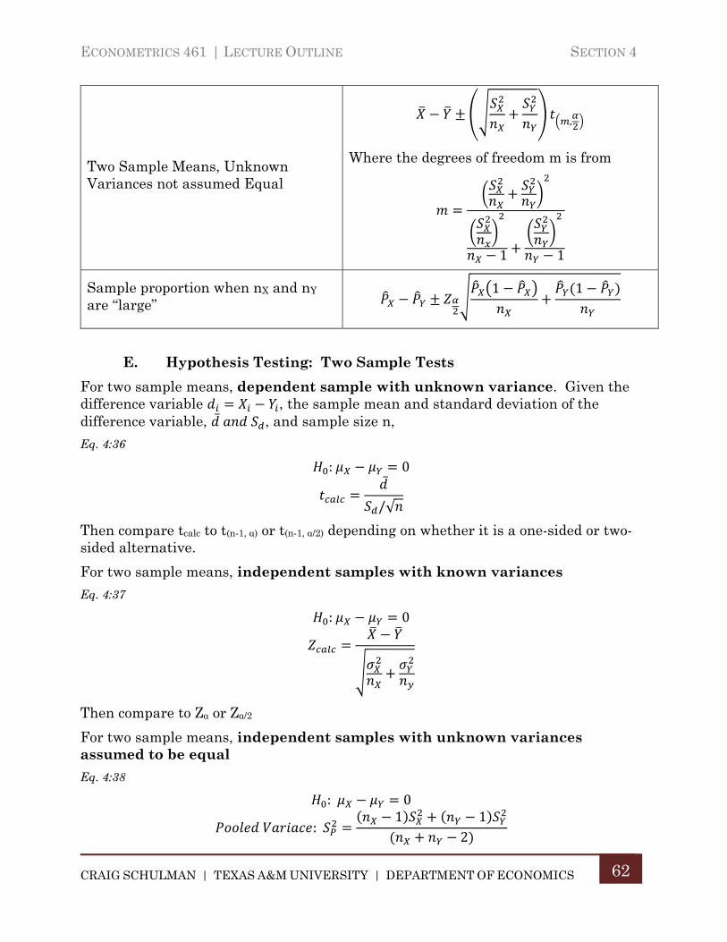
ECONOMETRICS 461 | LECTURE OUTLINE SECTION 4
CRAIG SCHULMAN | TEXAS A&M UNIVERSITY | DEPARTMENT OF ECONOMICS
62
Two Sample Means, Unknown Variances not assumed Equal
,
Where the degrees of freedom m is from
1 1
Sample proportion when nX and nY are “large”
1 1
E. Hypothesis Testing: Two Sample Tests
For two sample means, dependent sample with unknown variance. Given the difference variable , the sample mean and standard deviation of the difference variable, , and sample size n,
Eq. 4:36
: 0
/√
Then compare tcalc to t(n-1, α) or t(n-1, α/2) depending on whether it is a one-sided or two-sided alternative.
For two sample means, independent samples with known variances
Eq. 4:37
: 0
Then compare to Zα or Zα/2
For two sample means, independent samples with unknown variances assumed to be equal
Eq. 4:38
: 0
:1 1
2
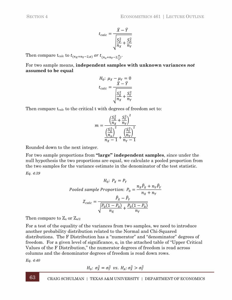
SECTION 4 ECONOMETRICS 461 | LECTURE OUTLINE
CRAIG SCHULMAN | TEXAS A&M UNIVERSITY | DEPARTMENT OF ECONOMICS
63
Then compare tcalc to , , .
For two sample means, independent samples with unknown variances not assumed to be equal
: 0
Then compare tcalc to the critical t with degrees of freedom set to:
1 1
Rounded down to the next integer.
For two sample proportions from “large” independent samples, since under the null hypothesis the two proportions are equal, we calculate a pooled proportion from the two samples for the variance estimate in the denominator of the test statistic.
Eq. 4:39
:
:
1 1
Then compare to Zα or Zα/2
For a test of the equality of the variances from two samples, we need to introduce another probability distribution related to the Normal and Chi-Squared distributions. The F Distribution has a “numerator” and “denominator” degrees of freedom. For a given level of significance, α, in the attached table of “Upper Critical Values of the F Distribution,” the numerator degrees of freedom is read across columns and the denominator degrees of freedom is read down rows.
Eq. 4:40
: . :
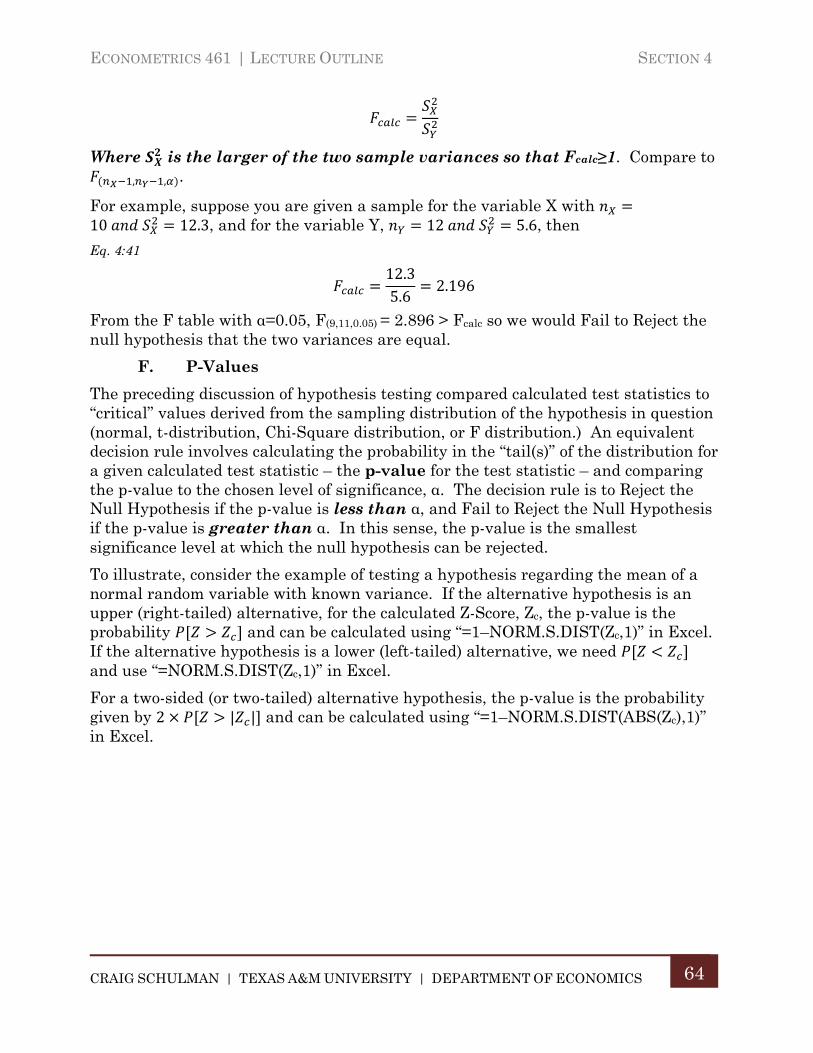
ECONOMETRICS 461 | LECTURE OUTLINE SECTION 4
CRAIG SCHULMAN | TEXAS A&M UNIVERSITY | DEPARTMENT OF ECONOMICS
64
Where is the larger of the two sample variances so that Fcalc≥1. Compare to , , .
For example, suppose you are given a sample for the variable X with 10 12.3, and for the variable Y, 12 5.6, then
Eq. 4:41
12.35.6
2.196
From the F table with α=0.05, F(9,11,0.05) = 2.896 > Fcalc so we would Fail to Reject the null hypothesis that the two variances are equal.
F. P-Values
The preceding discussion of hypothesis testing compared calculated test statistics to “critical” values derived from the sampling distribution of the hypothesis in question (normal, t-distribution, Chi-Square distribution, or F distribution.) An equivalent decision rule involves calculating the probability in the “tail(s)” of the distribution for a given calculated test statistic – the p-value for the test statistic – and comparing the p-value to the chosen level of significance, α. The decision rule is to Reject the Null Hypothesis if the p-value is less than α, and Fail to Reject the Null Hypothesis if the p-value is greater than α. In this sense, the p-value is the smallest significance level at which the null hypothesis can be rejected.
To illustrate, consider the example of testing a hypothesis regarding the mean of a normal random variable with known variance. If the alternative hypothesis is an upper (right-tailed) alternative, for the calculated Z-Score, Zc, the p-value is the probability and can be calculated using “=1–NORM.S.DIST(Zc,1)” in Excel. If the alternative hypothesis is a lower (left-tailed) alternative, we need and use “=NORM.S.DIST(Zc,1)” in Excel.
For a two-sided (or two-tailed) alternative hypothesis, the p-value is the probability given by 2 | | and can be calculated using “=1–NORM.S.DIST(ABS(Zc),1)” in Excel.
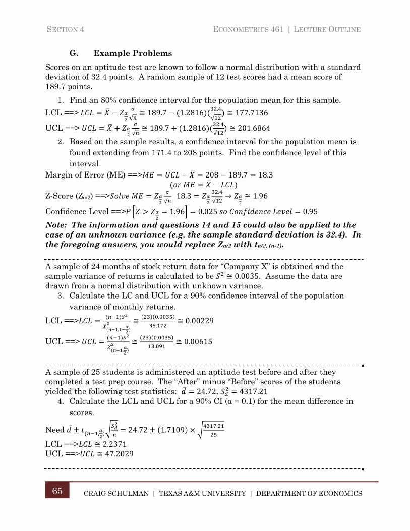
SECTION 4 ECONOMETRICS 461 | LECTURE OUTLINE
CRAIG SCHULMAN | TEXAS A&M UNIVERSITY | DEPARTMENT OF ECONOMICS
65
G. Example Problems
Scores on an aptitude test are known to follow a normal distribution with a standard deviation of 32.4 points. A random sample of 12 test scores had a mean score of 189.7 points.
1. Find an 80% confidence interval for the population mean for this sample.
LCL ==>√≅ 189.7 1.2816 .
√≅ 177.7136
UCL ==>√≅ 189.7 1.2816 .
√≅ 201.6864
2. Based on the sample results, a confidence interval for the population mean is found extending from 171.4 to 208 points. Find the confidence level of this interval.
Margin of Error (ME) ==> 208 189.7 18.3
Z-Score (Zα/2) ==> √18.3 .
√→ ≅ 1.96
Confidence Level ==> 1.96 0.025 0.95
Note: The information and questions 14 and 15 could also be applied to the case of an unknown variance (e.g. the sample standard deviation is 32.4). In the foregoing answers, you would replace Zα/2 with tα/2, (n-1).
A sample of 24 months of stock return data for “Company X” is obtained and the sample variance of returns is calculated to be ≅ 0.0035. Assume the data are drawn from a normal distribution with unknown variance.
3. Calculate the LC and UCL for a 90% confidence interval of the population variance of monthly returns.
LCL ==>,
≅ .
.≅ 0.00229
UCL ==>,
≅ .
.≅ 0.00615
A sample of 25 students is administered an aptitude test before and after they completed a test prep course. The “After” minus “Before” scores of the students yielded the following test statistics: 24.72, 4317.21
4. Calculate the LCL and UCL for a 90% CI (α = 0.1) for the mean difference in scores.
Need , 24.72 1.7109 .
LCL ==> ≅ 2.2371 UCL ==> ≅ 47.2029
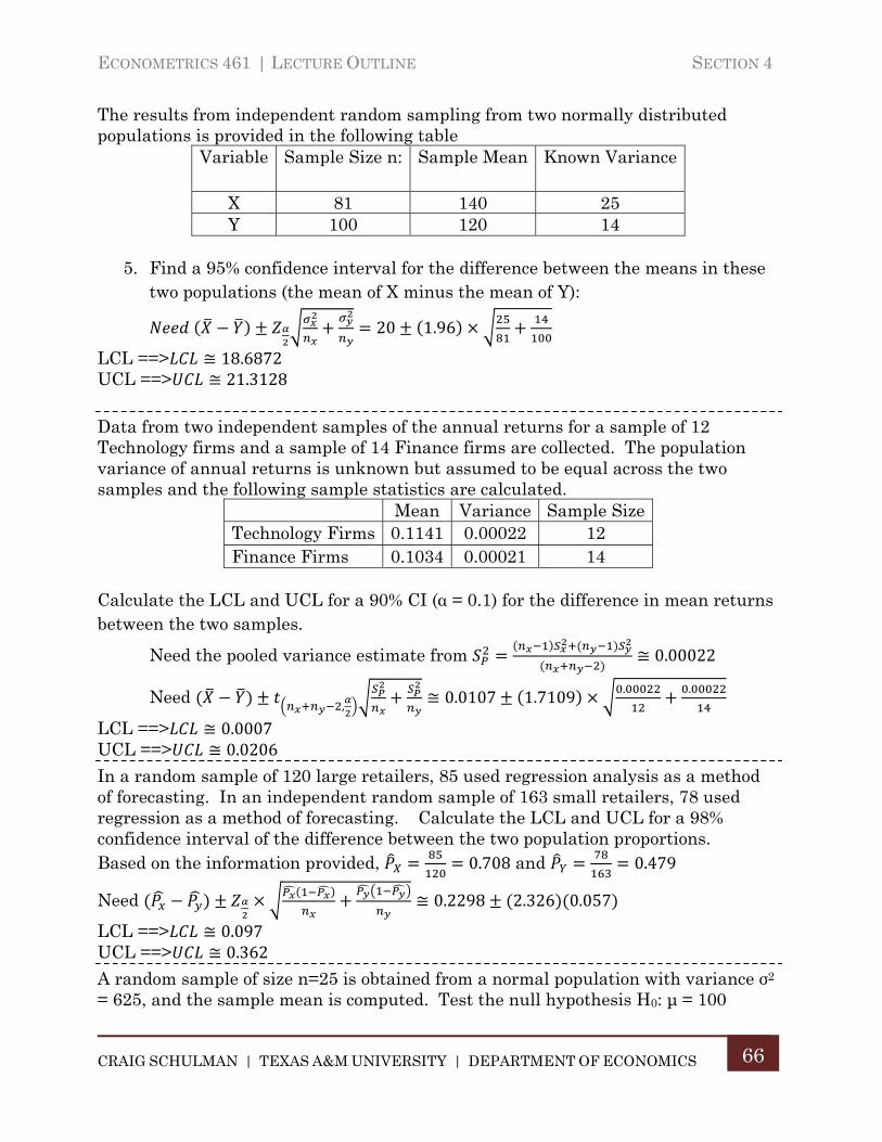
ECONOMETRICS 461 | LECTURE OUTLINE SECTION 4
CRAIG SCHULMAN | TEXAS A&M UNIVERSITY | DEPARTMENT OF ECONOMICS
66
The results from independent random sampling from two normally distributed populations is provided in the following table
Variable Sample Size n: Sample Mean Known Variance
X 81 140 25 Y 100 120 14
5. Find a 95% confidence interval for the difference between the means in these
two populations (the mean of X minus the mean of Y):
20 1.96
LCL ==> ≅ 18.6872 UCL ==> ≅ 21.3128
Data from two independent samples of the annual returns for a sample of 12 Technology firms and a sample of 14 Finance firms are collected. The population variance of annual returns is unknown but assumed to be equal across the two samples and the following sample statistics are calculated.
Mean Variance Sample Size Technology Firms 0.1141 0.00022 12 Finance Firms 0.1034 0.00021 14
Calculate the LCL and UCL for a 90% CI (α = 0.1) for the difference in mean returns between the two samples.
Need the pooled variance estimate from ≅ 0.00022
Need , ≅ 0.0107 1.7109 . .
LCL ==> ≅ 0.0007 UCL ==> ≅ 0.0206
In a random sample of 120 large retailers, 85 used regression analysis as a method of forecasting. In an independent random sample of 163 small retailers, 78 used regression as a method of forecasting. Calculate the LCL and UCL for a 98% confidence interval of the difference between the two population proportions. Based on the information provided, 0.708 and 0.479
Need ≅ 0.2298 2.326 0.057
LCL ==> ≅ 0.097 UCL ==> ≅ 0.362
A random sample of size n=25 is obtained from a normal population with variance σ2 = 625, and the sample mean is computed. Test the null hypothesis H0: μ = 100
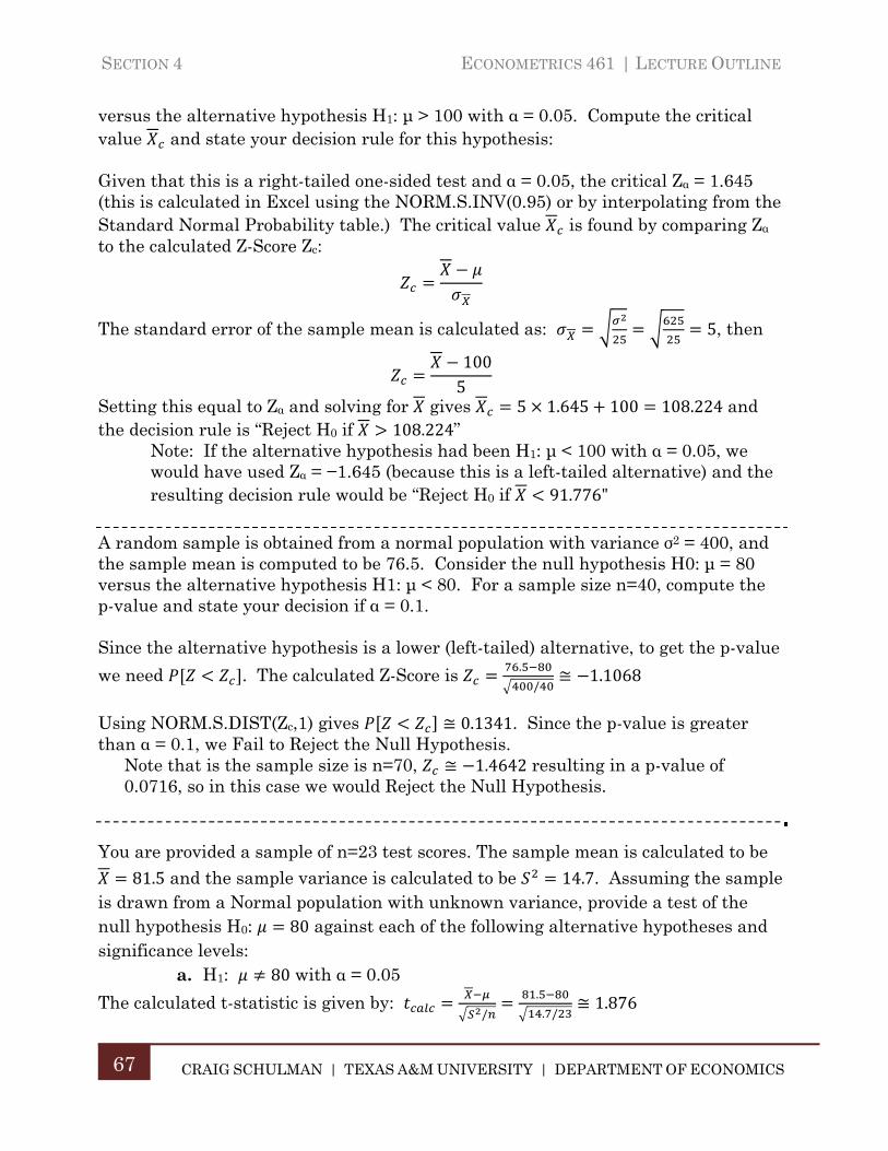
SECTION 4 ECONOMETRICS 461 | LECTURE OUTLINE
CRAIG SCHULMAN | TEXAS A&M UNIVERSITY | DEPARTMENT OF ECONOMICS
67
versus the alternative hypothesis H1: μ > 100 with α = 0.05. Compute the critical value and state your decision rule for this hypothesis:
Given that this is a right-tailed one-sided test and α = 0.05, the critical Zα = 1.645 (this is calculated in Excel using the NORM.S.INV(0.95) or by interpolating from the Standard Normal Probability table.) The critical value is found by comparing Zα to the calculated Z-Score Zc:
The standard error of the sample mean is calculated as: 5, then
1005
Setting this equal to Zα and solving for gives 5 1.645 100 108.224 and the decision rule is “Reject H0 if 108.224”
Note: If the alternative hypothesis had been H1: μ < 100 with α = 0.05, we would have used Zα = −1.645 (because this is a left-tailed alternative) and the resulting decision rule would be “Reject H0 if 91.776"
A random sample is obtained from a normal population with variance σ2 = 400, and the sample mean is computed to be 76.5. Consider the null hypothesis H0: μ = 80 versus the alternative hypothesis H1: μ < 80. For a sample size n=40, compute the p-value and state your decision if α = 0.1. Since the alternative hypothesis is a lower (left-tailed) alternative, to get the p-value
we need . The calculated Z-Score is .
/≅ 1.1068
Using NORM.S.DIST(Zc,1) gives ≅ 0.1341. Since the p-value is greater than α = 0.1, we Fail to Reject the Null Hypothesis.
Note that is the sample size is n=70, ≅ 1.4642 resulting in a p-value of 0.0716, so in this case we would Reject the Null Hypothesis.
You are provided a sample of n=23 test scores. The sample mean is calculated to be
81.5 and the sample variance is calculated to be 14.7. Assuming the sample is drawn from a Normal population with unknown variance, provide a test of the null hypothesis H0: 80 against each of the following alternative hypotheses and significance levels:
a. H1: 80 with α = 0.05
The calculated t-statistic is given by: /
.
. /≅ 1.876
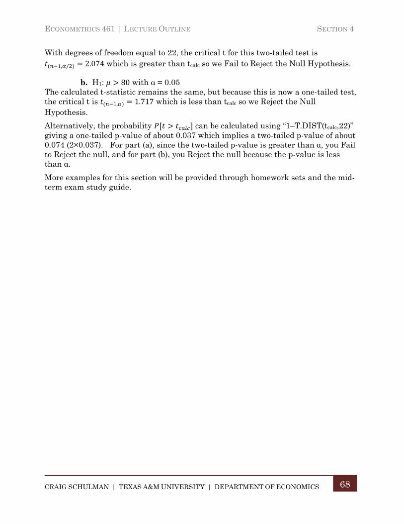
ECONOMETRICS 461 | LECTURE OUTLINE SECTION 4
CRAIG SCHULMAN | TEXAS A&M UNIVERSITY | DEPARTMENT OF ECONOMICS
68
With degrees of freedom equal to 22, the critical t for this two-tailed test is
, / 2.074 which is greater than tcalc so we Fail to Reject the Null Hypothesis.
b. H1: 80 with α = 0.05 The calculated t-statistic remains the same, but because this is now a one-tailed test, the critical t is , 1.717 which is less than tcalc so we Reject the Null Hypothesis.
Alternatively, the probability can be calculated using “1–T.DIST(tcalc,22)” giving a one-tailed p-value of about 0.037 which implies a two-tailed p-value of about 0.074 (2×0.037). For part (a), since the two-tailed p-value is greater than α, you Fail to Reject the null, and for part (b), you Reject the null because the p-value is less than α.
More examples for this section will be provided through homework sets and the mid-term exam study guide.
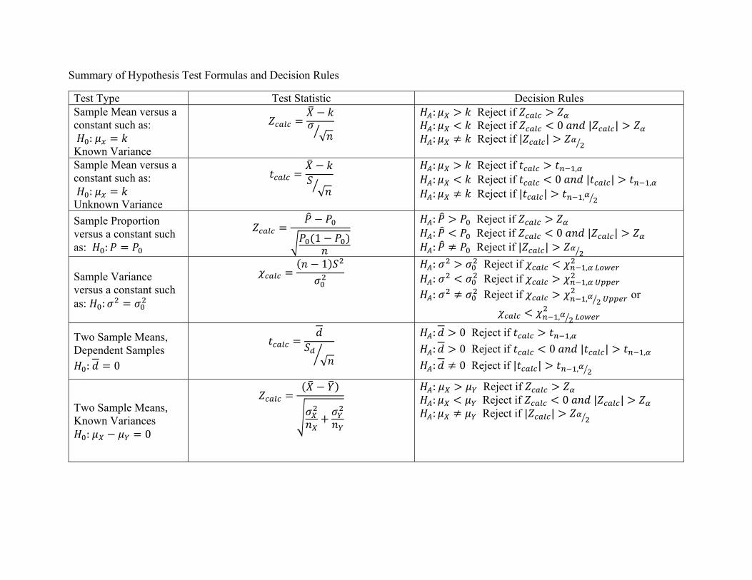
Summary of Hypothesis Test Formulas and Decision Rules
Test Type Test Statistic Decision Rules Sample Mean versus a constant such as: : Known Variance
√
: Reject if : Reject if 0 | | : Reject if | |
Sample Mean versus a constant such as: : Unknown Variance
√
: Reject if , : Reject if 0 | | , : Reject if | | ,
Sample Proportion versus a constant such as: :
1
: Reject if : Reject if 0 | | : Reject if | |
Sample Variance versus a constant such as: :
1
: Reject if , : Reject if ,
: Reject if , or
,
Two Sample Means, Dependent Samples : 0 √
: 0 Reject if ,
: 0 Reject if 0 | | ,
: 0 Reject if | | ,
Two Sample Means, Known Variances : 0
: Reject if : Reject if 0 | | : Reject if | |
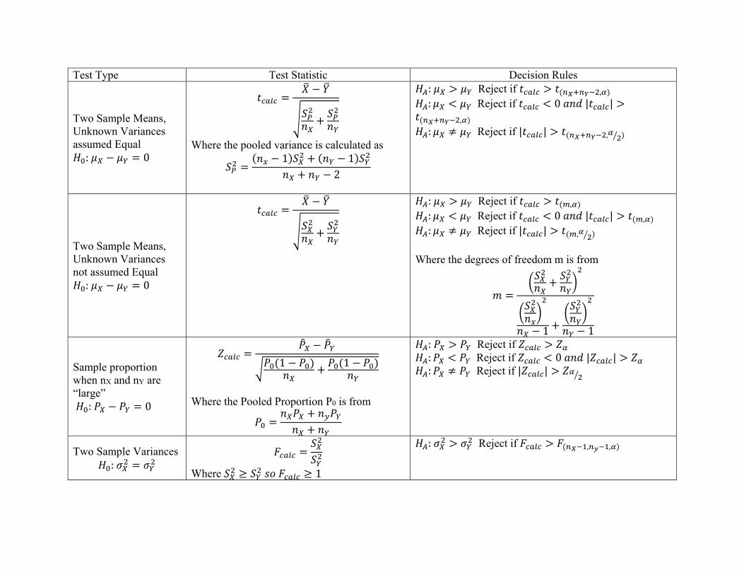
Test Type Test Statistic Decision Rules
Two Sample Means, Unknown Variances assumed Equal : 0
Where the pooled variance is calculated as 1 1
2
: Reject if , : Reject if 0 | |
, : Reject if | | ,
Two Sample Means, Unknown Variances not assumed Equal : 0
: Reject if , : Reject if 0 | | , : Reject if | | ,
Where the degrees of freedom m is from
1 1
Sample proportion when nX and nY are “large” : 0
1 1
Where the Pooled Proportion P0 is from
: Reject if : Reject if 0 | | : Reject if | |
Two Sample Variances :
Where 1
: Reject if , ,
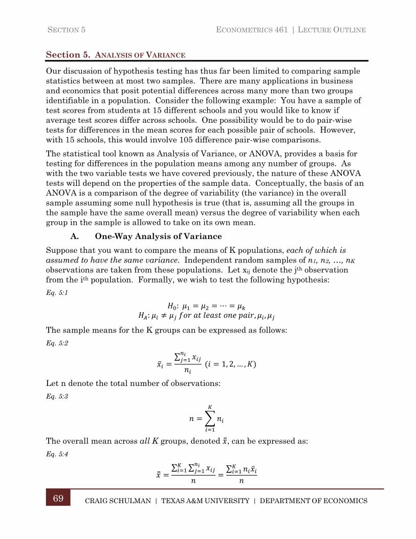
SECTION 5 ECONOMETRICS 461 | LECTURE OUTLINE
CRAIG SCHULMAN | TEXAS A&M UNIVERSITY | DEPARTMENT OF ECONOMICS
69
Section 5. ANALYSIS OF VARIANCE
Our discussion of hypothesis testing has thus far been limited to comparing sample statistics between at most two samples. There are many applications in business and economics that posit potential differences across many more than two groups identifiable in a population. Consider the following example: You have a sample of test scores from students at 15 different schools and you would like to know if average test scores differ across schools. One possibility would be to do pair-wise tests for differences in the mean scores for each possible pair of schools. However, with 15 schools, this would involve 105 difference pair-wise comparisons.
The statistical tool known as Analysis of Variance, or ANOVA, provides a basis for testing for differences in the population means among any number of groups. As with the two variable tests we have covered previously, the nature of these ANOVA tests will depend on the properties of the sample data. Conceptually, the basis of an ANOVA is a comparison of the degree of variability (the variance) in the overall sample assuming some null hypothesis is true (that is, assuming all the groups in the sample have the same overall mean) versus the degree of variability when each group in the sample is allowed to take on its own mean.
A. One-Way Analysis of Variance
Suppose that you want to compare the means of K populations, each of which is assumed to have the same variance. Independent random samples of n1, n2, …, nK observations are taken from these populations. Let xij denote the jth observation from the ith population. Formally, we wish to test the following hypothesis:
Eq. 5:1
: ⋯ : , ,
The sample means for the K groups can be expressed as follows:
Eq. 5:2
∑
1, 2, … ,
Let n denote the total number of observations:
Eq. 5:3
The overall mean across all K groups, denoted , can be expressed as:
Eq. 5:4
∑ ∑ ∑
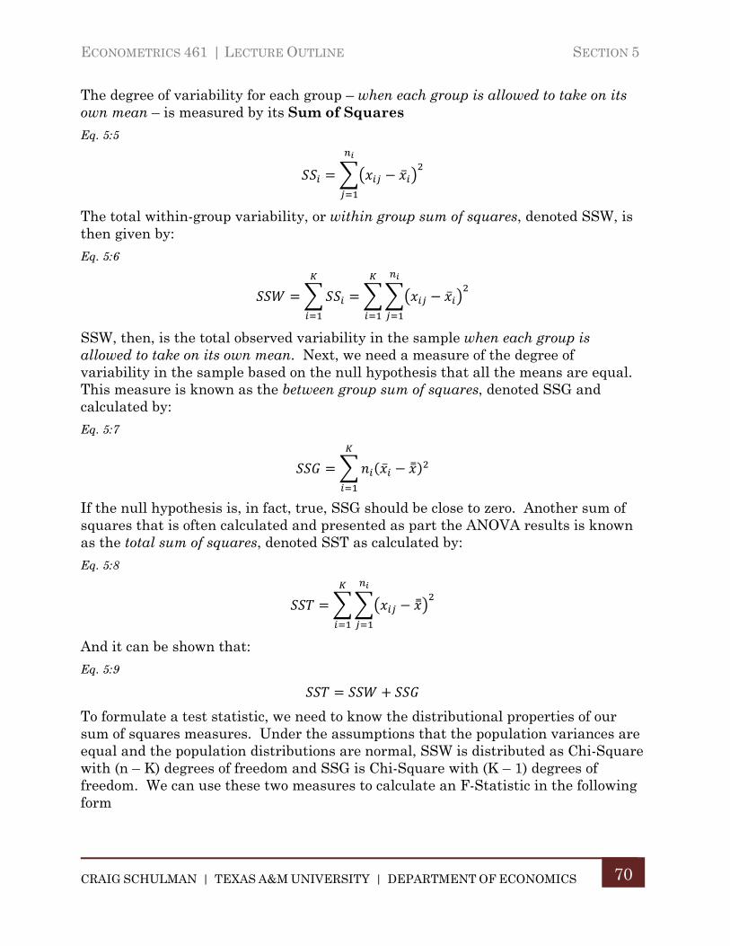
ECONOMETRICS 461 | LECTURE OUTLINE SECTION 5
CRAIG SCHULMAN | TEXAS A&M UNIVERSITY | DEPARTMENT OF ECONOMICS
70
The degree of variability for each group – when each group is allowed to take on its own mean – is measured by its Sum of Squares
Eq. 5:5
The total within-group variability, or within group sum of squares, denoted SSW, is then given by:
Eq. 5:6
SSW, then, is the total observed variability in the sample when each group is allowed to take on its own mean. Next, we need a measure of the degree of variability in the sample based on the null hypothesis that all the means are equal. This measure is known as the between group sum of squares, denoted SSG and calculated by:
Eq. 5:7
If the null hypothesis is, in fact, true, SSG should be close to zero. Another sum of squares that is often calculated and presented as part the ANOVA results is known as the total sum of squares, denoted SST as calculated by:
Eq. 5:8
And it can be shown that:
Eq. 5:9
To formulate a test statistic, we need to know the distributional properties of our sum of squares measures. Under the assumptions that the population variances are equal and the population distributions are normal, SSW is distributed as Chi-Square with (n – K) degrees of freedom and SSG is Chi-Square with (K – 1) degrees of freedom. We can use these two measures to calculate an F-Statistic in the following form
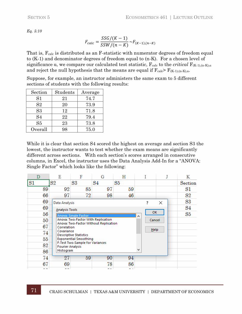
SECTION 5 ECONOMETRICS 461 | LECTURE OUTLINE
CRAIG SCHULMAN | TEXAS A&M UNIVERSITY | DEPARTMENT OF ECONOMICS
71
Eq. 5:10
/ 1/
~ ,
That is, Fcalc is distributed as an F-statistic with numerator degrees of freedom equal to (K-1) and denominator degrees of freedom equal to (n-K). For a chosen level of significance α, we compare our calculated test statistic, Fcalc to the critical F(K-1),(n-K),α and reject the null hypothesis that the means are equal if Fcalc> F(K-1),(n-K),α.
Suppose, for example, an instructor administers the same exam to 5 different sections of students with the following results:
Section Students Average S1 21 74.7 S2 20 73.9 S3 12 71.8 S4 22 79.4 S5 23 73.8
Overall 98 75.0
While it is clear that section S4 scored the highest on average and section S3 the lowest, the instructor wants to test whether the exam means are significantly different across sections. With each section’s scores arranged in consecutive columns, in Excel, the instructor uses the Data Analysis Add-In for a “ANOVA: Single Factor” which looks like the following:
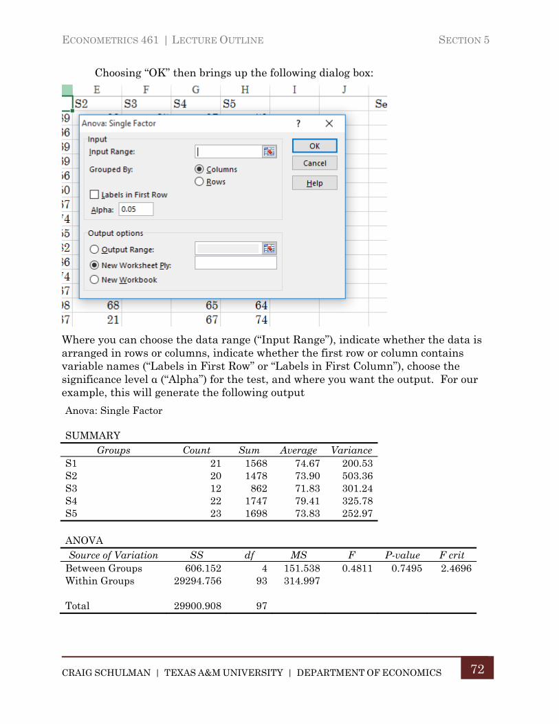
ECONOMETRICS 461 | LECTURE OUTLINE SECTION 5
CRAIG SCHULMAN | TEXAS A&M UNIVERSITY | DEPARTMENT OF ECONOMICS
72
Choosing “OK” then brings up the following dialog box:
Where you can choose the data range (“Input Range”), indicate whether the data is arranged in rows or columns, indicate whether the first row or column contains variable names (“Labels in First Row” or “Labels in First Column”), choose the significance level α (“Alpha”) for the test, and where you want the output. For our example, this will generate the following output
Anova: Single Factor
SUMMARY Groups Count Sum Average Variance
S1 21 1568 74.67 200.53 S2 20 1478 73.90 503.36 S3 12 862 71.83 301.24 S4 22 1747 79.41 325.78 S5 23 1698 73.83 252.97
ANOVA Source of Variation SS df MS F P-value F crit
Between Groups 606.152 4 151.538 0.4811 0.7495 2.4696 Within Groups 29294.756 93 314.997
Total 29900.908 97
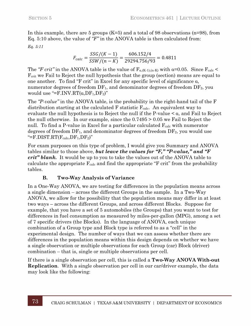
SECTION 5 ECONOMETRICS 461 | LECTURE OUTLINE
CRAIG SCHULMAN | TEXAS A&M UNIVERSITY | DEPARTMENT OF ECONOMICS
73
In this example, there are 5 groups (K=5) and a total of 98 observations (n=98), from Eq. 5:10 above, the value of “F” in the ANOVA table is then calculated from:
Eq. 5:11
/ 1/
606.152/429294.756/93
0.4811
The “F crit” in the ANOVA table is the value of Fα,(K-1),(n-K) with α=0.05. Since Fcalc < Fcrit we Fail to Reject the null hypothesis that the group (section) means are equal to one another. To find “F crit” in Excel for any specific level of significance α, numerator degrees of freedom DF1, and denominator degrees of freedom DF2, you would use “=F.INV.RT(α,DF1,DF2)”
The “P-value” in the ANOVA table, is the probability in the right-hand tail of the F distribution starting at the calculated F statistic Fcalc. An equivalent way to evaluate the null hypothesis is to Reject the null if the P-value < α, and Fail to Reject the null otherwise. In our example, since the 0.7495 > 0.05 we Fail to Reject the null. To find a P-value in Excel for a particular calculated Fcalc with numerator degrees of freedom DF1, and denominator degrees of freedom DF2, you would use “=F.DIST.RT(Fcalc,DF1,DF2)”
For exam purposes on this type of problem, I would give you Summary and ANOVA tables similar to those above, but leave the values for “F,” “P-value,” and “F crit” blank. It would be up to you to take the values out of the ANOVA table to calculate the appropriate Fcalc and find the appropriate “F crit” from the probability tables.
B. Two-Way Analysis of Variance
In a One-Way ANOVA, we are testing for differences in the population means across a single dimension – across the different Groups in the sample. In a Two-Way ANOVA, we allow for the possibility that the population means may differ in at least two ways – across the different Groups, and across different Blocks. Suppose for example, that you have a set of 5 automobiles (the Groups) that you want to test for differences in fuel consumption as measured by miles-per-gallon (MPG), among a set of 7 specific drivers (the Blocks). In the language of ANOVA, each unique combination of a Group type and Block type is referred to as a “cell” in the experimental design. The number of ways that we can assess whether there are differences in the population means within this design depends on whether we have a single observation or multiple observations for each Group (car) Block (driver) combination – that is, single or multiple observations per cell.
If there is a single observation per cell, this is called a Two-Way ANOVA With-out Replication. With a single observation per cell in our car/driver example, the data may look like the following:
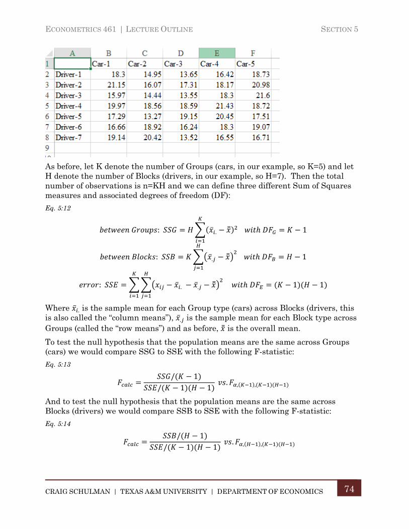
ECONOMETRICS 461 | LECTURE OUTLINE SECTION 5
CRAIG SCHULMAN | TEXAS A&M UNIVERSITY | DEPARTMENT OF ECONOMICS
74
As before, let K denote the number of Groups (cars, in our example, so K=5) and let H denote the number of Blocks (drivers, in our example, so H=7). Then the total number of observations is n=KH and we can define three different Sum of Squares measures and associated degrees of freedom (DF):
Eq. 5:12
: . 1
: . 1
: . . 1 1
Where . is the sample mean for each Group type (cars) across Blocks (drivers, this is also called the “column means”), . is the sample mean for each Block type across Groups (called the “row means”) and as before, is the overall mean.
To test the null hypothesis that the population means are the same across Groups (cars) we would compare SSG to SSE with the following F-statistic:
Eq. 5:13
/ 1/ 1 1
. , ,
And to test the null hypothesis that the population means are the same across Blocks (drivers) we would compare SSB to SSE with the following F-statistic:
Eq. 5:14
/ 1/ 1 1
. , ,
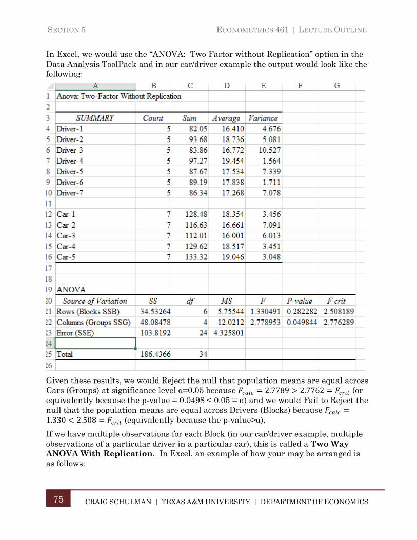
SECTION 5 ECONOMETRICS 461 | LECTURE OUTLINE
CRAIG SCHULMAN | TEXAS A&M UNIVERSITY | DEPARTMENT OF ECONOMICS
75
In Excel, we would use the “ANOVA: Two Factor without Replication” option in the Data Analysis ToolPack and in our car/driver example the output would look like the following:
Given these results, we would Reject the null that population means are equal across Cars (Groups) at significance level α=0.05 because 2.7789 2.7762 (or equivalently because the p-value = 0.0498 < 0.05 = α) and we would Fail to Reject the null that the population means are equal across Drivers (Blocks) because 1.330 2.508 (equivalently because the p-value>α).
If we have multiple observations for each Block (in our car/driver example, multiple observations of a particular driver in a particular car), this is called a Two Way ANOVA With Replication. In Excel, an example of how your may be arranged is as follows:
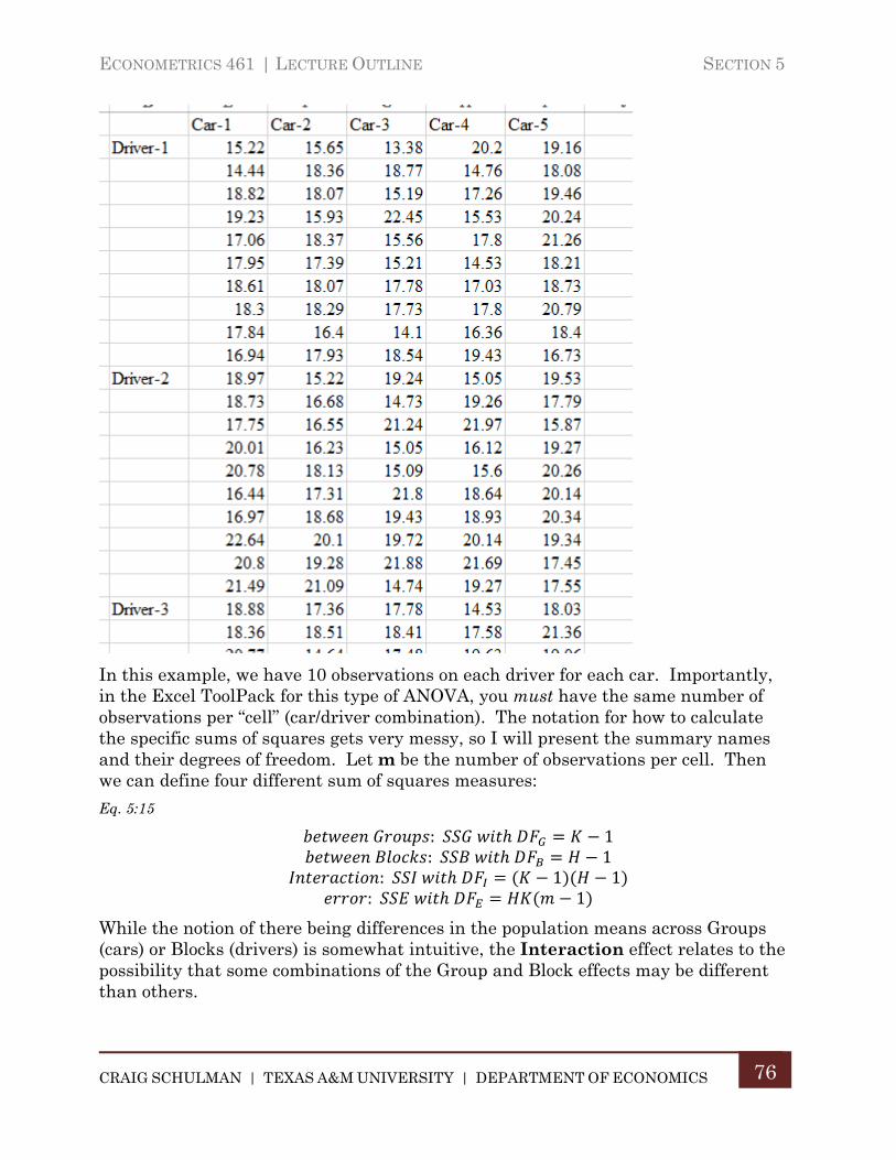
ECONOMETRICS 461 | LECTURE OUTLINE SECTION 5
CRAIG SCHULMAN | TEXAS A&M UNIVERSITY | DEPARTMENT OF ECONOMICS
76
In this example, we have 10 observations on each driver for each car. Importantly, in the Excel ToolPack for this type of ANOVA, you must have the same number of observations per “cell” (car/driver combination). The notation for how to calculate the specific sums of squares gets very messy, so I will present the summary names and their degrees of freedom. Let m be the number of observations per cell. Then we can define four different sum of squares measures:
Eq. 5:15
: 1 : 1: 1 1
: 1
While the notion of there being differences in the population means across Groups (cars) or Blocks (drivers) is somewhat intuitive, the Interaction effect relates to the possibility that some combinations of the Group and Block effects may be different than others.
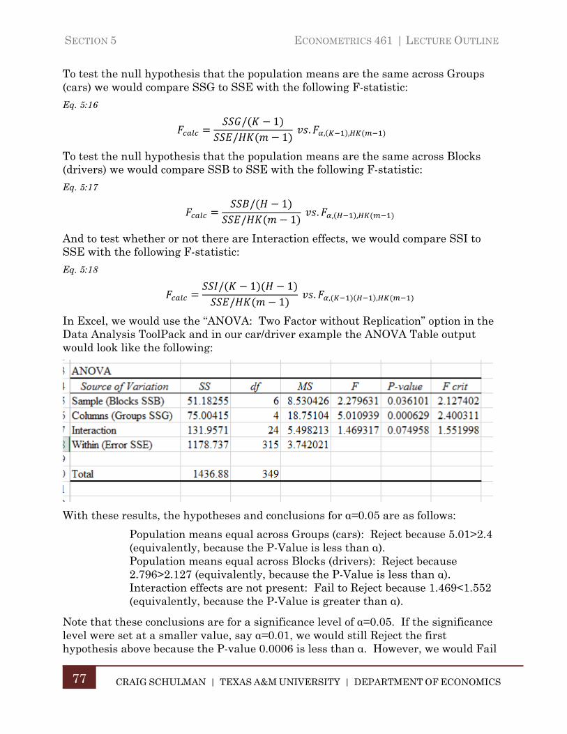
SECTION 5 ECONOMETRICS 461 | LECTURE OUTLINE
CRAIG SCHULMAN | TEXAS A&M UNIVERSITY | DEPARTMENT OF ECONOMICS
77
To test the null hypothesis that the population means are the same across Groups (cars) we would compare SSG to SSE with the following F-statistic:
Eq. 5:16
/ 1/ 1
. , ,
To test the null hypothesis that the population means are the same across Blocks (drivers) we would compare SSB to SSE with the following F-statistic:
Eq. 5:17
/ 1/ 1
. , ,
And to test whether or not there are Interaction effects, we would compare SSI to SSE with the following F-statistic:
Eq. 5:18
/ 1 1/ 1
. , ,
In Excel, we would use the “ANOVA: Two Factor without Replication” option in the Data Analysis ToolPack and in our car/driver example the ANOVA Table output would look like the following:
With these results, the hypotheses and conclusions for α=0.05 are as follows:
Population means equal across Groups (cars): Reject because 5.01>2.4 (equivalently, because the P-Value is less than α). Population means equal across Blocks (drivers): Reject because 2.796>2.127 (equivalently, because the P-Value is less than α). Interaction effects are not present: Fail to Reject because 1.469<1.552 (equivalently, because the P-Value is greater than α).
Note that these conclusions are for a significance level of α=0.05. If the significance level were set at a smaller value, say α=0.01, we would still Reject the first hypothesis above because the P-value 0.0006 is less than α. However, we would Fail

ECONOMETRICS 461 | LECTURE OUTLINE SECTION 5
CRAIG SCHULMAN | TEXAS A&M UNIVERSITY | DEPARTMENT OF ECONOMICS
78
to Reject the second hypothesis because the P-value 0.036 is now greater than α. Similarly, if we set α=0.1, we would Reject the hypothesis that there are no Interaction effects because it’s P-value of 0.075 is less than α.
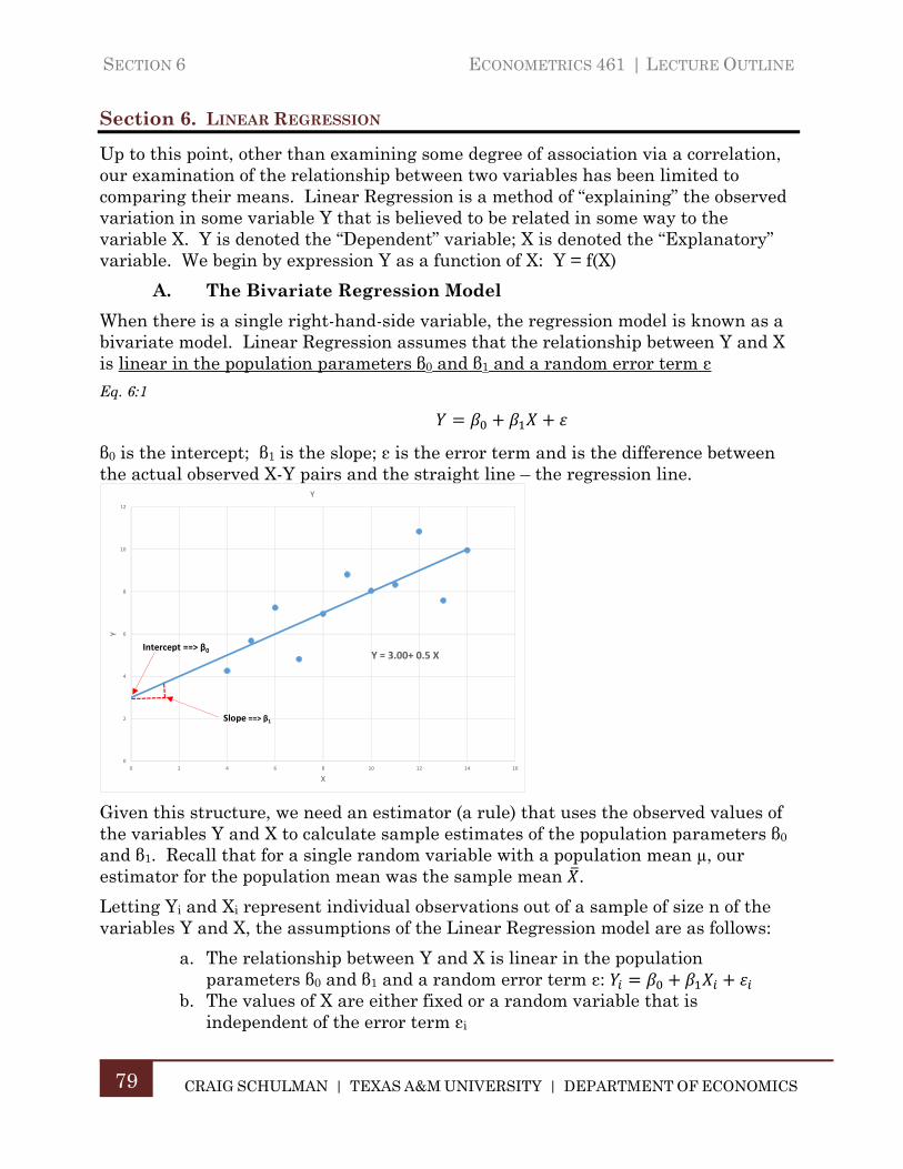
SECTION 6 ECONOMETRICS 461 | LECTURE OUTLINE
CRAIG SCHULMAN | TEXAS A&M UNIVERSITY | DEPARTMENT OF ECONOMICS
79
Section 6. LINEAR REGRESSION
Up to this point, other than examining some degree of association via a correlation, our examination of the relationship between two variables has been limited to comparing their means. Linear Regression is a method of “explaining” the observed variation in some variable Y that is believed to be related in some way to the variable X. Y is denoted the “Dependent” variable; X is denoted the “Explanatory” variable. We begin by expression Y as a function of X: Y = f(X)
A. The Bivariate Regression Model
When there is a single right-hand-side variable, the regression model is known as a bivariate model. Linear Regression assumes that the relationship between Y and X is linear in the population parameters β0 and β1 and a random error term ε
Eq. 6:1
β0 is the intercept; β1 is the slope; ε is the error term and is the difference between the actual observed X-Y pairs and the straight line – the regression line.
Given this structure, we need an estimator (a rule) that uses the observed values of the variables Y and X to calculate sample estimates of the population parameters β0 and β1. Recall that for a single random variable with a population mean µ, our estimator for the population mean was the sample mean .
Letting Yi and Xi represent individual observations out of a sample of size n of the variables Y and X, the assumptions of the Linear Regression model are as follows:
a. The relationship between Y and X is linear in the population parameters β0 and β1 and a random error term ε:
b. The values of X are either fixed or a random variable that is independent of the error term εi
Y = 3.00+ 0.5 X
0
2
4
6
8
10
12
0 2 4 6 8 10 12 14 16
Y
X
Y
Intercept ==> β0
Slope ==> β1
ECONOMETRICS 461 | LECTURE OUTLINE SECTION 6
CRAIG SCHULMAN | TEXAS A&M UNIVERSITY | DEPARTMENT OF ECONOMICS
80
c. The random error term εi is distributed with a mean of zero and a constant variance σ2: εi ~ (0, σ2)
The estimator that we will use to calculation sample estimates for the population parameters β0 and β1 and a random error term ε is the Least Squares Procedure which is based on finding the sample estimators b0 (for β0) and b1 (for β1) that minimize the Sum of Squared Errors – SSE – defined as follows:
Eq. 6:2
Taking derivatives of SSE with respect to b0 and b1, setting them equal to zero and solving for b0 and b1 gives (after some manipulation) the following Least Squares estimators of β0 and β1
Eq. 6:3
∑
∑
The Least Squares estimator of the random error term is:
Eq. 6:4
.
Note that so long as the regression equation includes an intercept term, b0, the Least Squares procedure will give the result: ∑ 0. The Least Squares Estimator for the variance of ε, σ2 is denoted S2 and given by:
Eq. 6:5
2
Given the assumptions of the Least Squares procedure in (4) above, the Least Squares Estimators b0 and b1 are Unbiased:
Eq. 6:6
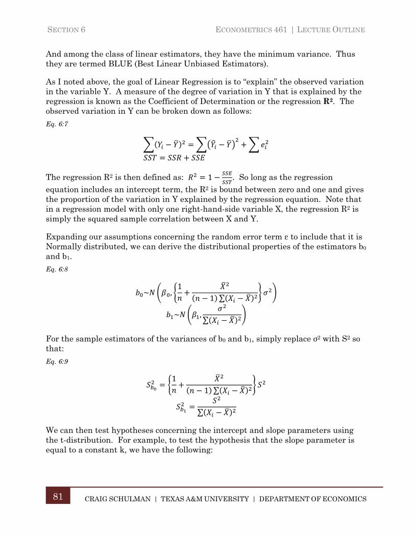
SECTION 6 ECONOMETRICS 461 | LECTURE OUTLINE
CRAIG SCHULMAN | TEXAS A&M UNIVERSITY | DEPARTMENT OF ECONOMICS
81
And among the class of linear estimators, they have the minimum variance. Thus they are termed BLUE (Best Linear Unbiased Estimators).
As I noted above, the goal of Linear Regression is to “explain” the observed variation in the variable Y. A measure of the degree of variation in Y that is explained by the regression is known as the Coefficient of Determination or the regression R2. The observed variation in Y can be broken down as follows:
Eq. 6:7
The regression R2 is then defined as: 1 . So long as the regression equation includes an intercept term, the R2 is bound between zero and one and gives the proportion of the variation in Y explained by the regression equation. Note that in a regression model with only one right-hand-side variable X, the regression R2 is simply the squared sample correlation between X and Y.
Expanding our assumptions concerning the random error term ε to include that it is Normally distributed, we can derive the distributional properties of the estimators b0 and b1.
Eq. 6:8
~ ,1
1 ∑
~ ,∑
For the sample estimators of the variances of b0 and b1, simply replace σ2 with S2 so that:
Eq. 6:9
11 ∑
∑
We can then test hypotheses concerning the intercept and slope parameters using the t-distribution. For example, to test the hypothesis that the slope parameter is equal to a constant k, we have the following:
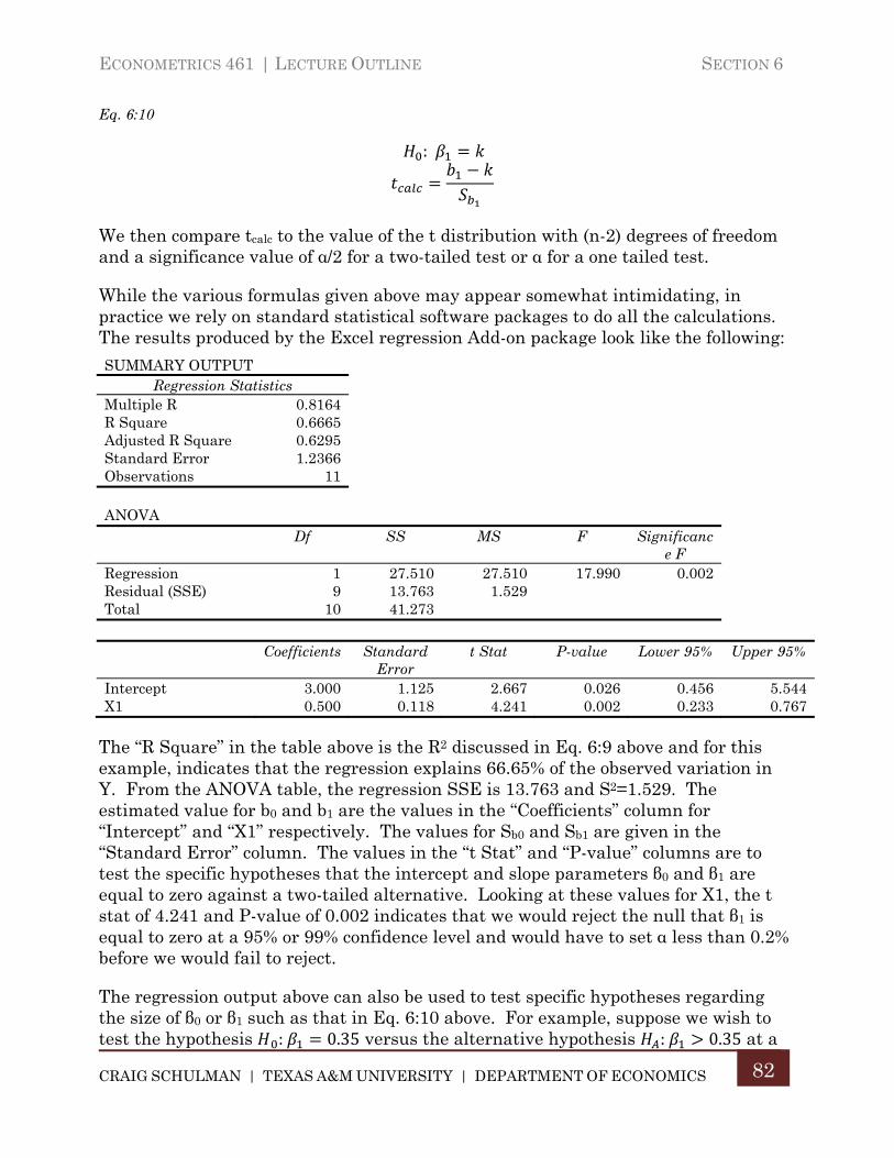
ECONOMETRICS 461 | LECTURE OUTLINE SECTION 6
CRAIG SCHULMAN | TEXAS A&M UNIVERSITY | DEPARTMENT OF ECONOMICS
82
Eq. 6:10
:
We then compare tcalc to the value of the t distribution with (n-2) degrees of freedom and a significance value of α/2 for a two-tailed test or α for a one tailed test.
While the various formulas given above may appear somewhat intimidating, in practice we rely on standard statistical software packages to do all the calculations. The results produced by the Excel regression Add-on package look like the following:
SUMMARY OUTPUT Regression Statistics
Multiple R 0.8164 R Square 0.6665 Adjusted R Square 0.6295 Standard Error 1.2366 Observations 11
ANOVA
Df SS MS F Significance F
Regression 1 27.510 27.510 17.990 0.002 Residual (SSE) 9 13.763 1.529 Total 10 41.273
Coefficients Standard
Error t Stat P-value Lower 95% Upper 95%
Intercept 3.000 1.125 2.667 0.026 0.456 5.544 X1 0.500 0.118 4.241 0.002 0.233 0.767
The “R Square” in the table above is the R2 discussed in Eq. 6:9 above and for this example, indicates that the regression explains 66.65% of the observed variation in Y. From the ANOVA table, the regression SSE is 13.763 and S2=1.529. The estimated value for b0 and b1 are the values in the “Coefficients” column for “Intercept” and “X1” respectively. The values for Sb0 and Sb1 are given in the “Standard Error” column. The values in the “t Stat” and “P-value” columns are to test the specific hypotheses that the intercept and slope parameters β0 and β1 are equal to zero against a two-tailed alternative. Looking at these values for X1, the t stat of 4.241 and P-value of 0.002 indicates that we would reject the null that β1 is equal to zero at a 95% or 99% confidence level and would have to set α less than 0.2% before we would fail to reject.
The regression output above can also be used to test specific hypotheses regarding the size of β0 or β1 such as that in Eq. 6:10 above. For example, suppose we wish to test the hypothesis : 0.35 versus the alternative hypothesis : 0.35 at a
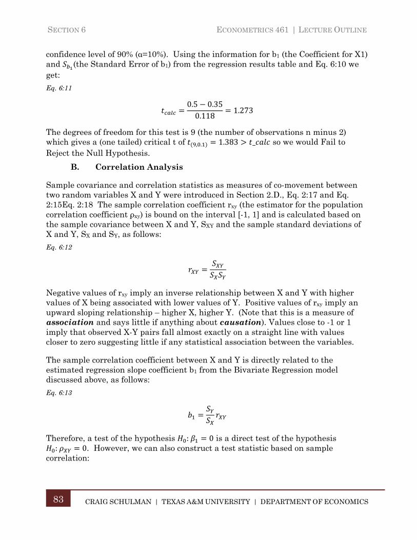
SECTION 6 ECONOMETRICS 461 | LECTURE OUTLINE
CRAIG SCHULMAN | TEXAS A&M UNIVERSITY | DEPARTMENT OF ECONOMICS
83
confidence level of 90% (α=10%). Using the information for b1 (the Coefficient for X1) and (the Standard Error of b1) from the regression results table and Eq. 6:10 we get:
Eq. 6:11
0.5 0.350.118
1.273
The degrees of freedom for this test is 9 (the number of observations n minus 2) which gives a (one tailed) critical t of , . 1.383 _ so we would Fail to Reject the Null Hypothesis.
B. Correlation Analysis
Sample covariance and correlation statistics as measures of co-movement between two random variables X and Y were introduced in Section 2.D., Eq. 2:17 and Eq. 2:15Eq. 2:18 The sample correlation coefficient rxy (the estimator for the population correlation coefficient ρxy) is bound on the interval [-1, 1] and is calculated based on the sample covariance between X and Y, SXY and the sample standard deviations of X and Y, SX and SY, as follows:
Eq. 6:12
Negative values of rxy imply an inverse relationship between X and Y with higher values of X being associated with lower values of Y. Positive values of rxy imply an upward sloping relationship – higher X, higher Y. (Note that this is a measure of association and says little if anything about causation). Values close to -1 or 1 imply that observed X-Y pairs fall almost exactly on a straight line with values closer to zero suggesting little if any statistical association between the variables.
The sample correlation coefficient between X and Y is directly related to the estimated regression slope coefficient b1 from the Bivariate Regression model discussed above, as follows:
Eq. 6:13
Therefore, a test of the hypothesis : 0 is a direct test of the hypothesis : 0. However, we can also construct a test statistic based on sample
correlation:
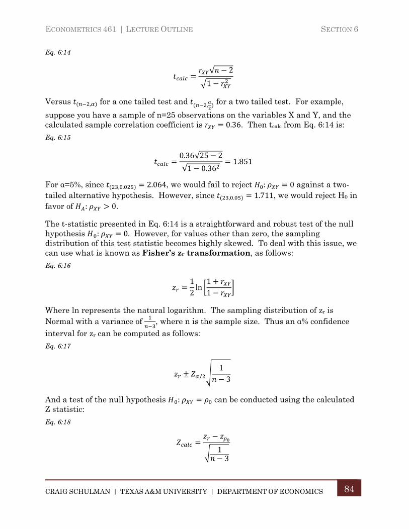
ECONOMETRICS 461 | LECTURE OUTLINE SECTION 6
CRAIG SCHULMAN | TEXAS A&M UNIVERSITY | DEPARTMENT OF ECONOMICS
84
Eq. 6:14
√ 2
1
Versus , for a one tailed test and , for a two tailed test. For example,
suppose you have a sample of n=25 observations on the variables X and Y, and the calculated sample correlation coefficient is 0.36. Then tcalc from Eq. 6:14 is:
Eq. 6:15
0.36√25 2
√1 0.361.851
For α=5%, since , . 2.064, we would fail to reject : 0 against a two-tailed alternative hypothesis. However, since , . 1.711, we would reject H0 in favor of : 0.
The t-statistic presented in Eq. 6:14 is a straightforward and robust test of the null hypothesis : 0. However, for values other than zero, the sampling distribution of this test statistic becomes highly skewed. To deal with this issue, we can use what is known as Fisher’s zr transformation, as follows:
Eq. 6:16
12ln
11
Where ln represents the natural logarithm. The sampling distribution of zr is Normal with a variance of , where n is the sample size. Thus an α% confidence interval for zr can be computed as follows:
Eq. 6:17
/13
And a test of the null hypothesis : can be conducted using the calculated Z statistic:
Eq. 6:18
13
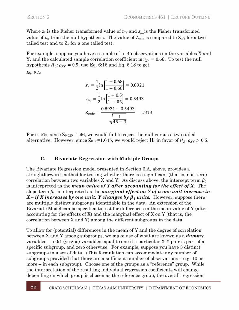
SECTION 6 ECONOMETRICS 461 | LECTURE OUTLINE
CRAIG SCHULMAN | TEXAS A&M UNIVERSITY | DEPARTMENT OF ECONOMICS
85
Where zr is the Fisher transformed value of rxy and is the Fisher transformed value of from the null hypothesis. The value of Zcalc is compared to Zα/2 for a two-tailed test and to Zα for a one tailed test.
For example, suppose you have a sample of n=45 observations on the variables X and Y, and the calculated sample correlation coefficient is 0.68. To test the null hypothesis : 0.5, use Eq. 6:16 and Eq. 6:18 to get:
Eq. 6:19
12ln
1 0.681 0.68
0.8921
12ln
1 0.51 .05
0.5493
0.8921 0.5493
145 3
1.813
For α=5%, since Z0.025=1.96, we would fail to reject the null versus a two tailed alternative. However, since Z0.05=1.645, we would reject H0 in favor of : 0.5.
C. Bivariate Regression with Multiple Groups
The Bivariate Regression model presented in Section 6.A, above, provides a straightforward method for testing whether there is a significant (that is, non-zero) correlation between two variables X and Y. As discuss above, the intercept term is interpreted as the mean value of Y after accounting for the effect of X. The slope term is interpreted as the marginal effect on Y of a one unit increase in X – if X increases by one unit, Y changes by units. However, suppose there are multiple distinct subgroups identifiable in the data. An extension of the Bivariate Model can be specified to test for differences in the mean value of Y (after accounting for the effects of X) and the marginal effect of X on Y (that is, the correlation between X and Y) among the different subgroups in the data.
To allow for (potential) differences in the mean of Y and the degree of correlation between X and Y among subgroups, we make use of what are known as a dummy variables – a 0/1 (yes/no) variables equal to one if a particular X-Y pair is part of a specific subgroup, and zero otherwise. For example, suppose you have 3 distinct subgroups in a set of data. (This formulation can accommodate any number of subgroups provided that there are a sufficient number of observations – e.g. 10 or more – in each subgroup). Choose one of the groups as a “reference” group. While the interpretation of the resulting individual regression coefficients will change depending on which group is chosen as the reference group, the overall regression
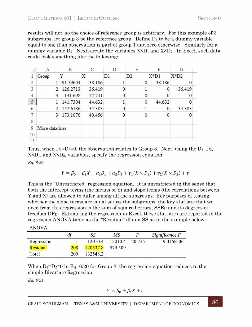
ECONOMETRICS 461 | LECTURE OUTLINE SECTION 6
CRAIG SCHULMAN | TEXAS A&M UNIVERSITY | DEPARTMENT OF ECONOMICS
86
results will not, so the choice of reference group is arbitrary. For this example of 3 subgroups, let group 3 be the reference group. Define D1 to be a dummy variable equal to one if an observation is part of group 1 and zero otherwise. Similarly for a dummy variable D2. Next, create the variables X×D1 and X×D2. In Excel, such data could look something like the following:
Thus, when D1=D2=0, the observation relates to Group 3. Next, using the D1, D2, X×D1, and X×D2, variables, specify the regression equation:
Eq. 6:20
This is the “Unrestricted” regression equation. It is unrestricted in the sense that both the intercept terms (the means of Y) and slope terms (the correlations between Y and X) are allowed to differ among all the subgroups. For purposes of testing whether the slope terms are equal across the subgroups, the key statistic that we need from this regression is the sum of squared errors, SSEU and its degrees of freedom DFU. Estimating the regression in Excel, these statistics are reported in the regression ANOVA table as the “Residual” df and SS as in the example below:
ANOVA
df SS MS F Significance F Regression 1 12010.4 12010.4 20.725 9.016E-06 Residual 208 120537.8 579.509 Total 209 132548.2
When D1=D2=0 in Eq. 6:20 for Group 3, the regression equation reduces to the simple Bivariate Regression:
Eq. 6:21
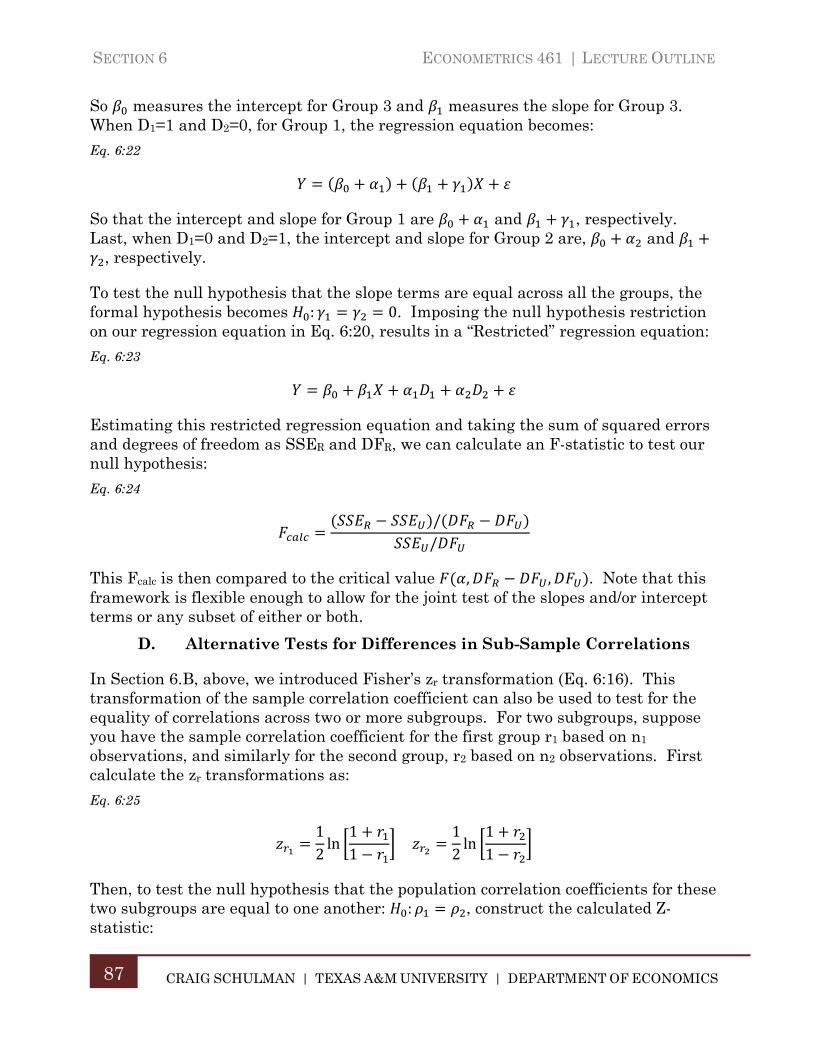
SECTION 6 ECONOMETRICS 461 | LECTURE OUTLINE
CRAIG SCHULMAN | TEXAS A&M UNIVERSITY | DEPARTMENT OF ECONOMICS
87
So measures the intercept for Group 3 and measures the slope for Group 3. When D1=1 and D2=0, for Group 1, the regression equation becomes:
Eq. 6:22
So that the intercept and slope for Group 1 are and , respectively. Last, when D1=0 and D2=1, the intercept and slope for Group 2 are, and
, respectively.
To test the null hypothesis that the slope terms are equal across all the groups, the formal hypothesis becomes : 0. Imposing the null hypothesis restriction on our regression equation in Eq. 6:20, results in a “Restricted” regression equation:
Eq. 6:23
Estimating this restricted regression equation and taking the sum of squared errors and degrees of freedom as SSER and DFR, we can calculate an F-statistic to test our null hypothesis:
Eq. 6:24
//
This Fcalc is then compared to the critical value , , . Note that this framework is flexible enough to allow for the joint test of the slopes and/or intercept terms or any subset of either or both.
D. Alternative Tests for Differences in Sub-Sample Correlations
In Section 6.B, above, we introduced Fisher’s zr transformation (Eq. 6:16). This transformation of the sample correlation coefficient can also be used to test for the equality of correlations across two or more subgroups. For two subgroups, suppose you have the sample correlation coefficient for the first group r1 based on n1 observations, and similarly for the second group, r2 based on n2 observations. First calculate the zr transformations as:
Eq. 6:25
12ln
11
12ln
11
Then, to test the null hypothesis that the population correlation coefficients for these two subgroups are equal to one another: : , construct the calculated Z-statistic:
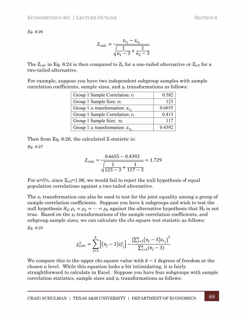
ECONOMETRICS 461 | LECTURE OUTLINE SECTION 6
CRAIG SCHULMAN | TEXAS A&M UNIVERSITY | DEPARTMENT OF ECONOMICS
88
Eq. 6:26
13
13
The Zcalc in Eq. 6:24 is then compared to Zα for a one-tailed alternative or Zα/2 for a two-tailed alternative.
For example, suppose you have two independent subgroup samples with sample correlation coefficients, sample sizes, and zr transformations as follows:
Group 1 Sample Correlation: r1 0.582 Group 1 Sample Size: n1 123 Group 1 zr transformation: 0.6655 Group 1 Sample Correlation: r2 0.413 Group 1 Sample Size: n2 117
Group 1 zr transformation: 0.4392
Then from Eq. 6:26, the calculated Z-statistic is:
Eq. 6:27
0.6655 0.4392
1123 3
1117 3
1.729
For α=5%, since Zα/2=1.96, we would fail to reject the null hypothesis of equal population correlations against a two-tailed alternative.
The zr transformation can also be used to test for the joint equality among a group of sample correlation coefficients. Suppose you have k subgroups and wish to test the null hypothesis : ⋯ against the alternative hypothesis that H0 is not true. Based on the zr transformations of the sample correlation coefficients, and subgroup sample sizes, we can calculate the chi-square test statistic as follows:
Eq. 6:28
3∑ 3
∑ 3
We compare this to the upper chi-square value with 1 degrees of freedom at the chosen α level. While this equation looks a bit intimidating, it is fairly straightforward to calculate in Excel. Suppose you have four subgroups with sample correlation statistics, sample sizes and zr transformations as follows:
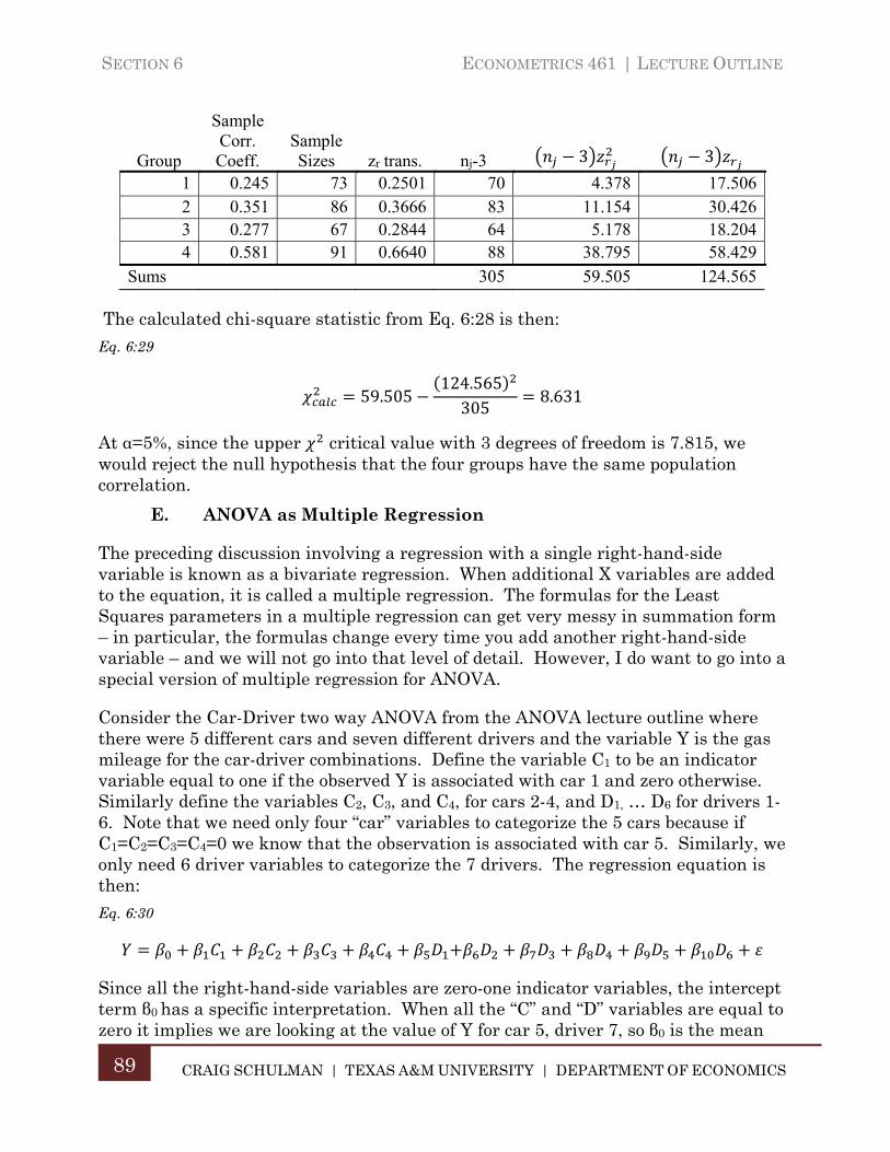
SECTION 6 ECONOMETRICS 461 | LECTURE OUTLINE
CRAIG SCHULMAN | TEXAS A&M UNIVERSITY | DEPARTMENT OF ECONOMICS
89
Group
Sample Corr. Coeff.
Sample Sizes zr trans. nj-3 3 3
1 0.245 73 0.2501 70 4.378 17.506 2 0.351 86 0.3666 83 11.154 30.426 3 0.277 67 0.2844 64 5.178 18.204 4 0.581 91 0.6640 88 38.795 58.429
Sums 305 59.505 124.565
The calculated chi-square statistic from Eq. 6:28 is then:
Eq. 6:29
59.505124.565305
8.631
At α=5%, since the upper critical value with 3 degrees of freedom is 7.815, we would reject the null hypothesis that the four groups have the same population correlation.
E. ANOVA as Multiple Regression
The preceding discussion involving a regression with a single right-hand-side variable is known as a bivariate regression. When additional X variables are added to the equation, it is called a multiple regression. The formulas for the Least Squares parameters in a multiple regression can get very messy in summation form – in particular, the formulas change every time you add another right-hand-side variable – and we will not go into that level of detail. However, I do want to go into a special version of multiple regression for ANOVA.
Consider the Car-Driver two way ANOVA from the ANOVA lecture outline where there were 5 different cars and seven different drivers and the variable Y is the gas mileage for the car-driver combinations. Define the variable C1 to be an indicator variable equal to one if the observed Y is associated with car 1 and zero otherwise. Similarly define the variables C2, C3, and C4, for cars 2-4, and D1, … D6 for drivers 1-6. Note that we need only four “car” variables to categorize the 5 cars because if C1=C2=C3=C4=0 we know that the observation is associated with car 5. Similarly, we only need 6 driver variables to categorize the 7 drivers. The regression equation is then:
Eq. 6:30
Since all the right-hand-side variables are zero-one indicator variables, the intercept term β0 has a specific interpretation. When all the “C” and “D” variables are equal to zero it implies we are looking at the value of Y for car 5, driver 7, so β0 is the mean
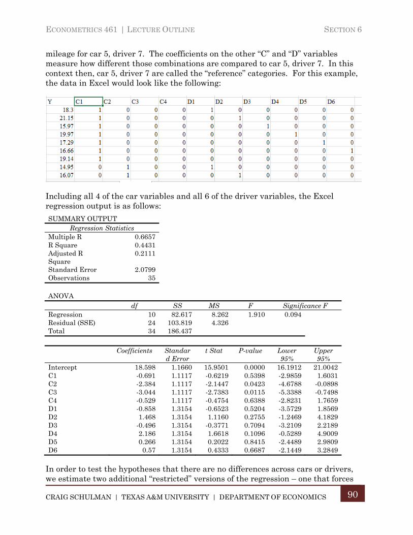
ECONOMETRICS 461 | LECTURE OUTLINE SECTION 6
CRAIG SCHULMAN | TEXAS A&M UNIVERSITY | DEPARTMENT OF ECONOMICS
90
mileage for car 5, driver 7. The coefficients on the other “C” and “D” variables measure how different those combinations are compared to car 5, driver 7. In this context then, car 5, driver 7 are called the “reference” categories. For this example, the data in Excel would look like the following:
Including all 4 of the car variables and all 6 of the driver variables, the Excel regression output is as follows:
SUMMARY OUTPUT Regression Statistics
Multiple R 0.6657 R Square 0.4431 Adjusted R Square
0.2111
Standard Error 2.0799 Observations 35
ANOVA
df SS MS F Significance F Regression 10 82.617 8.262 1.910 0.094 Residual (SSE) 24 103.819 4.326 Total 34 186.437
Coefficients Standar
d Error t Stat P-value Lower
95% Upper 95%
Intercept 18.598 1.1660 15.9501 0.0000 16.1912 21.0042 C1 -0.691 1.1117 -0.6219 0.5398 -2.9859 1.6031 C2 -2.384 1.1117 -2.1447 0.0423 -4.6788 -0.0898 C3 -3.044 1.1117 -2.7383 0.0115 -5.3388 -0.7498 C4 -0.529 1.1117 -0.4754 0.6388 -2.8231 1.7659 D1 -0.858 1.3154 -0.6523 0.5204 -3.5729 1.8569 D2 1.468 1.3154 1.1160 0.2755 -1.2469 4.1829 D3 -0.496 1.3154 -0.3771 0.7094 -3.2109 2.2189 D4 2.186 1.3154 1.6618 0.1096 -0.5289 4.9009 D5 0.266 1.3154 0.2022 0.8415 -2.4489 2.9809 D6 0.57 1.3154 0.4333 0.6687 -2.1449 3.2849
In order to test the hypotheses that there are no differences across cars or drivers, we estimate two additional “restricted” versions of the regression – one that forces
SECTION 6 ECONOMETRICS 461 | LECTURE OUTLINE
CRAIG SCHULMAN | TEXAS A&M UNIVERSITY | DEPARTMENT OF ECONOMICS
91
all the car effects to be zero (it leaves out the car variables) and another that forces all the driver effects to be zero. The general form of the test statistic for these hypotheses is as follows:
Eq. 6:31
//
~ ,
Where SSEU is the SSE from the “unrestricted” regression above, DFU is the degrees of freedom for the unrestricted regression, SSER is the SSE from a regression that “restricts” either the car effects or the driver effects to be zero. For this example, the ANOVA tables from the two “restricted” regressions are as follows:
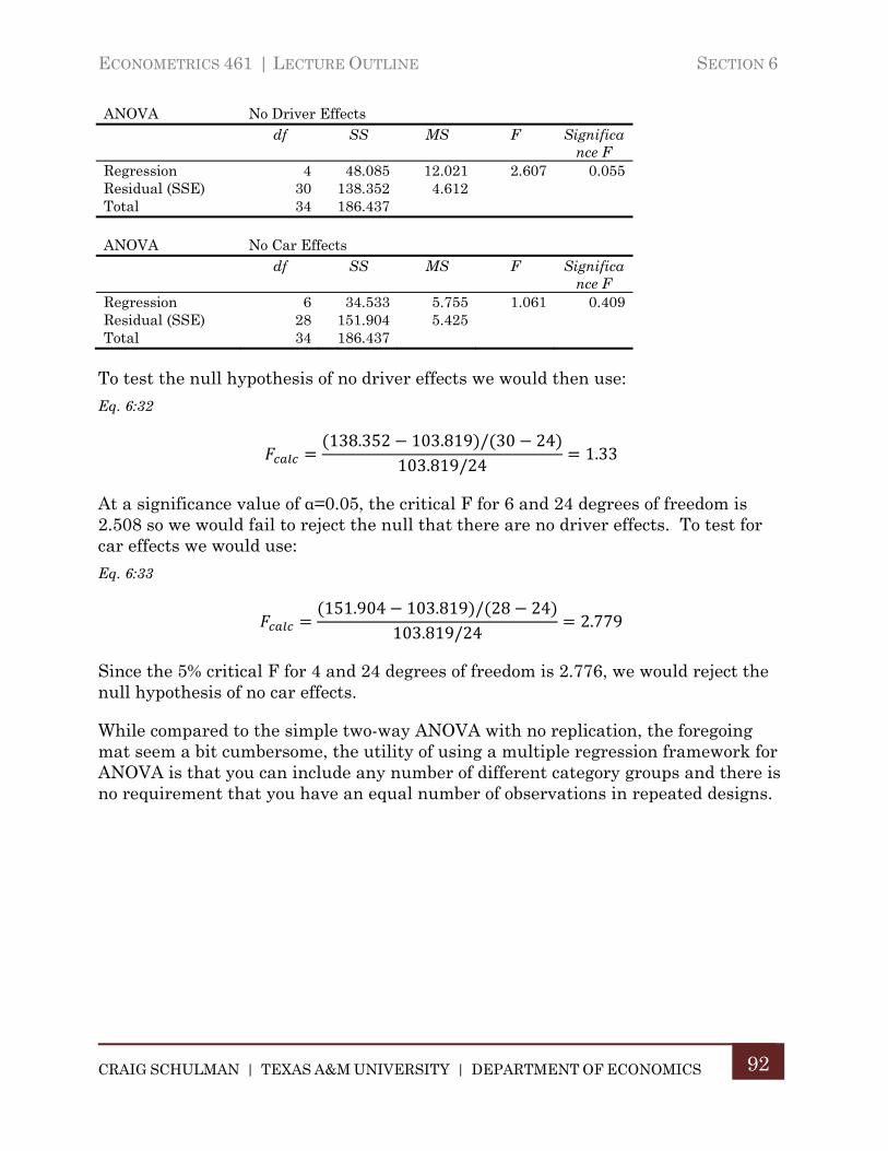
ECONOMETRICS 461 | LECTURE OUTLINE SECTION 6
CRAIG SCHULMAN | TEXAS A&M UNIVERSITY | DEPARTMENT OF ECONOMICS
92
ANOVA No Driver Effects df SS MS F Significa
nce F Regression 4 48.085 12.021 2.607 0.055 Residual (SSE) 30 138.352 4.612 Total 34 186.437
ANOVA No Car Effects
df SS MS F Significance F
Regression 6 34.533 5.755 1.061 0.409 Residual (SSE) 28 151.904 5.425 Total 34 186.437
To test the null hypothesis of no driver effects we would then use:
Eq. 6:32
138.352 103.819 / 30 24103.819/24
1.33
At a significance value of α=0.05, the critical F for 6 and 24 degrees of freedom is 2.508 so we would fail to reject the null that there are no driver effects. To test for car effects we would use:
Eq. 6:33
151.904 103.819 / 28 24103.819/24
2.779
Since the 5% critical F for 4 and 24 degrees of freedom is 2.776, we would reject the null hypothesis of no car effects.
While compared to the simple two-way ANOVA with no replication, the foregoing mat seem a bit cumbersome, the utility of using a multiple regression framework for ANOVA is that you can include any number of different category groups and there is no requirement that you have an equal number of observations in repeated designs.
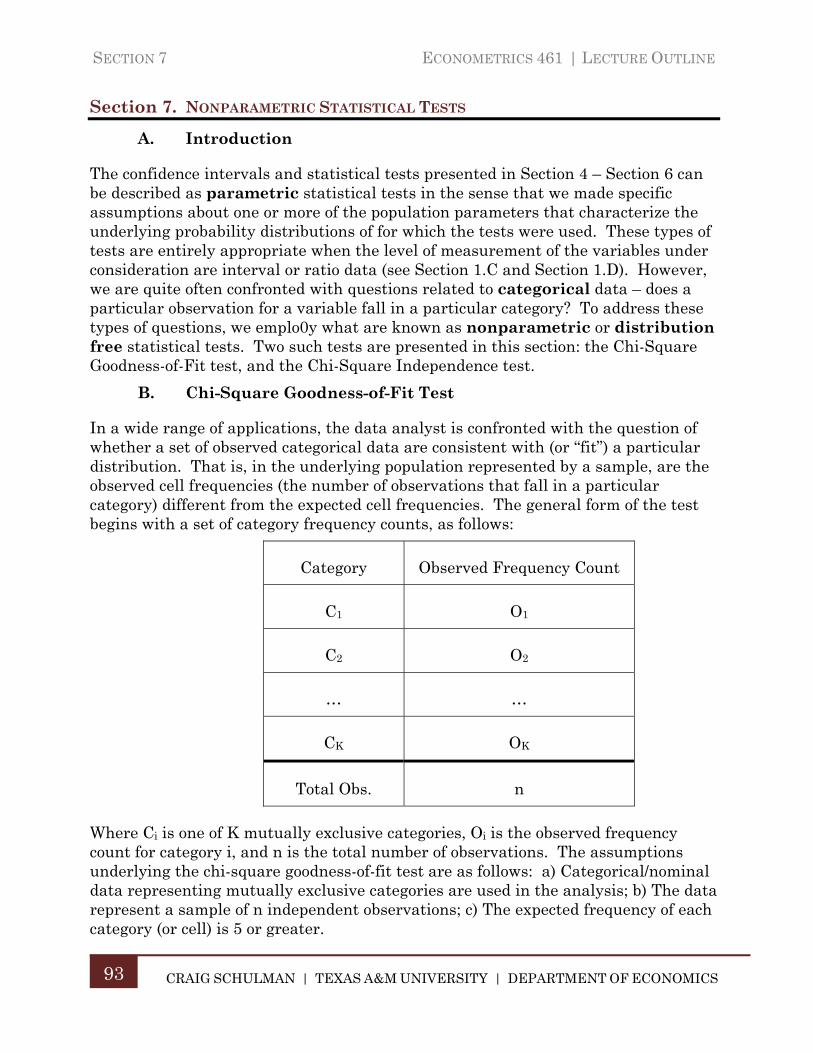
SECTION 7 ECONOMETRICS 461 | LECTURE OUTLINE
CRAIG SCHULMAN | TEXAS A&M UNIVERSITY | DEPARTMENT OF ECONOMICS
93
Section 7. NONPARAMETRIC STATISTICAL TESTS
A. Introduction
The confidence intervals and statistical tests presented in Section 4 – Section 6 can be described as parametric statistical tests in the sense that we made specific assumptions about one or more of the population parameters that characterize the underlying probability distributions of for which the tests were used. These types of tests are entirely appropriate when the level of measurement of the variables under consideration are interval or ratio data (see Section 1.C and Section 1.D). However, we are quite often confronted with questions related to categorical data – does a particular observation for a variable fall in a particular category? To address these types of questions, we emplo0y what are known as nonparametric or distribution free statistical tests. Two such tests are presented in this section: the Chi-Square Goodness-of-Fit test, and the Chi-Square Independence test.
B. Chi-Square Goodness-of-Fit Test
In a wide range of applications, the data analyst is confronted with the question of whether a set of observed categorical data are consistent with (or “fit”) a particular distribution. That is, in the underlying population represented by a sample, are the observed cell frequencies (the number of observations that fall in a particular category) different from the expected cell frequencies. The general form of the test begins with a set of category frequency counts, as follows:
Category Observed Frequency Count
C1 O1
C2 O2
… …
CK OK
Total Obs. n
Where Ci is one of K mutually exclusive categories, Oi is the observed frequency count for category i, and n is the total number of observations. The assumptions underlying the chi-square goodness-of-fit test are as follows: a) Categorical/nominal data representing mutually exclusive categories are used in the analysis; b) The data represent a sample of n independent observations; c) The expected frequency of each category (or cell) is 5 or greater.

ECONOMETRICS 461 | LECTURE OUTLINE SECTION 7
CRAIG SCHULMAN | TEXAS A&M UNIVERSITY | DEPARTMENT OF ECONOMICS
94
If there are K different categories of outcomes, Oi is the number of observed outcomes for category i, and Ei is the number of expected outcomes for category i (based on the distribution postulated in the null hypothesis), the null hypothesis to be tested is, : for all K categories, versus the alternative hypothesis : for at least one category. The following chi-square statistic then provides
a test of the null hypothesis that the data are consistent with (“fit”) the hypothesized distribution:
Eq. 7:1
This is distributed as and is always evaluated as a one-tailed (upper or right hand value) alternative. Thus we would reject the null hypothesis if
, . For example, suppose you have data that reflect 5 different categories of outcomes, with observed and expected outcomes as follows:
Category Observed Expected
1 35 50 4.50 2 40 30 3.33 3 20 12 5.33 4 1 6 4.17 5 4 2 2.00
19.33
For 0.05, the upper critical value 9.49 so we would reject the null hypothesis.
This type of test can be used for many types of discrete probability distributions. As another example, suppose you roll a six-sided die 120 times and wish to test whether the die is “fair.” With a fair die, the probability of any individual outcome {1, 2, …, 6} on a particular roll is 1/6. Thus, with a sample of n=120 rolls, the expected frequency of each possible outcome under the null hypothesis of a “fair” die is: 120 20. Using the framework above, suppose you observe outcome frequencies as shown in the following table:
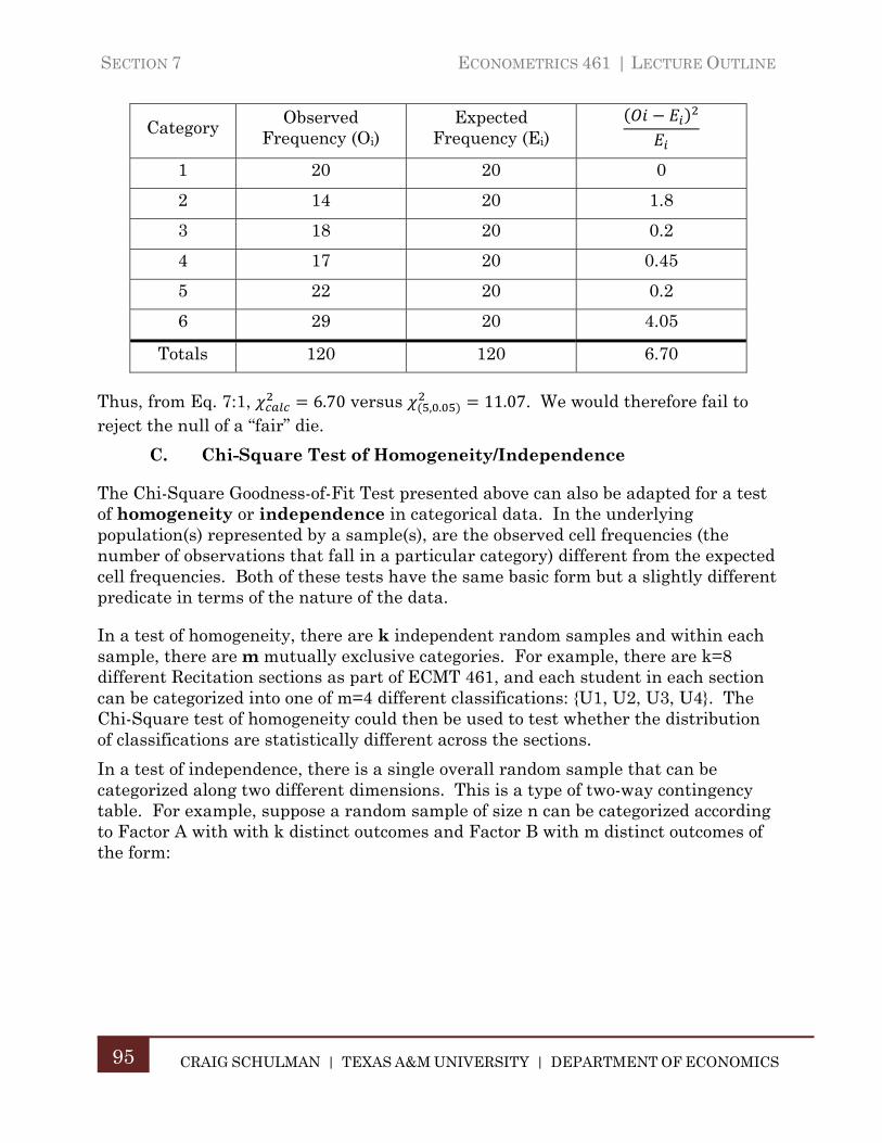
SECTION 7 ECONOMETRICS 461 | LECTURE OUTLINE
CRAIG SCHULMAN | TEXAS A&M UNIVERSITY | DEPARTMENT OF ECONOMICS
95
Category Observed Frequency (Oi)
Expected Frequency (Ei)
1 20 20 0
2 14 20 1.8
3 18 20 0.2
4 17 20 0.45
5 22 20 0.2
6 29 20 4.05
Totals 120 120 6.70
Thus, from Eq. 7:1, 6.70 versus , . 11.07. We would therefore fail to reject the null of a “fair” die.
C. Chi-Square Test of Homogeneity/Independence
The Chi-Square Goodness-of-Fit Test presented above can also be adapted for a test of homogeneity or independence in categorical data. In the underlying population(s) represented by a sample(s), are the observed cell frequencies (the number of observations that fall in a particular category) different from the expected cell frequencies. Both of these tests have the same basic form but a slightly different predicate in terms of the nature of the data.
In a test of homogeneity, there are k independent random samples and within each sample, there are m mutually exclusive categories. For example, there are k=8 different Recitation sections as part of ECMT 461, and each student in each section can be categorized into one of m=4 different classifications: {U1, U2, U3, U4}. The Chi-Square test of homogeneity could then be used to test whether the distribution of classifications are statistically different across the sections.
In a test of independence, there is a single overall random sample that can be categorized along two different dimensions. This is a type of two-way contingency table. For example, suppose a random sample of size n can be categorized according to Factor A with with k distinct outcomes and Factor B with m distinct outcomes of the form:
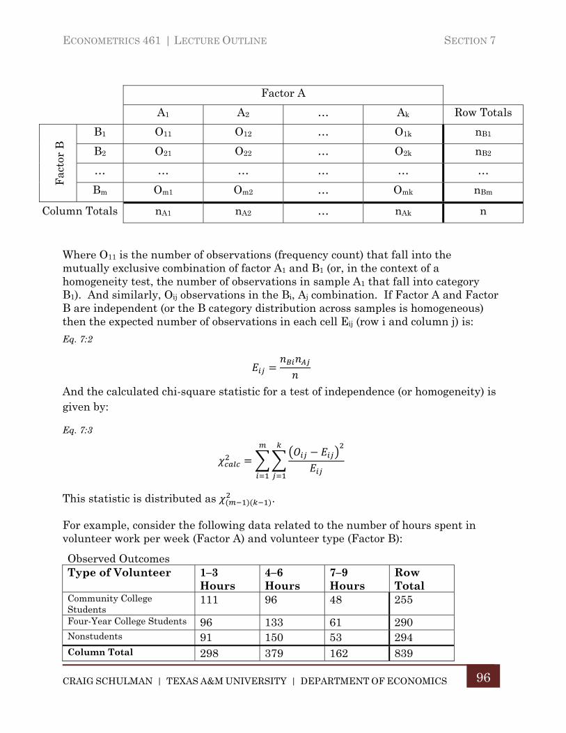
ECONOMETRICS 461 | LECTURE OUTLINE SECTION 7
CRAIG SCHULMAN | TEXAS A&M UNIVERSITY | DEPARTMENT OF ECONOMICS
96
Factor A
A1 A2 … Ak Row Totals
B1 O11 O12 … O1k nB1
B2 O21 O22 … O2k nB2
… … … … … …
Bm Om1 Om2 … Omk nBm
Column Totals nA1 nA2 … nAk n
Where O11 is the number of observations (frequency count) that fall into the mutually exclusive combination of factor A1 and B1 (or, in the context of a homogeneity test, the number of observations in sample A1 that fall into category B1). And similarly, Oij observations in the Bi, Aj combination. If Factor A and Factor B are independent (or the B category distribution across samples is homogeneous) then the expected number of observations in each cell Eij (row i and column j) is:
Eq. 7:2
And the calculated chi-square statistic for a test of independence (or homogeneity) is given by:
Eq. 7:3
This statistic is distributed as .
For example, consider the following data related to the number of hours spent in volunteer work per week (Factor A) and volunteer type (Factor B):
Observed Outcomes Type of Volunteer 1–3
Hours 4–6 Hours
7–9 Hours
Row Total
Community College Students
111 96 48 255
Four-Year College Students 96 133 61 290 Nonstudents 91 150 53 294 Column Total 298 379 162 839
Fac
tor
B

SECTION 7 ECONOMETRICS 461 | LECTURE OUTLINE
CRAIG SCHULMAN | TEXAS A&M UNIVERSITY | DEPARTMENT OF ECONOMICS
97
Based on these data, we can calculate Expected Outcomes under the null hypothesis of independence:
Expected Outcomes Type of Volunteer 1–3
Hours 4–6 Hours
7–9 Hours
Row Total
Community College Students
91 115 49 255
Four-Year College Students 103 131 56 290 Nonstudents 104 133 57 294 Column Total 298 379 162 839
And the elements of the test statistic:
4.607 3.197 0.031 0.476 0.030 0.447 1.726 2.225 0.250
12.991
Since there are 3 of each factor type, this statistic is distributed as – chi-squared with 4 degrees of freedom. At α=0.05, the critical value is 9.488, and we would therefore reject the null hypothesis of independence.

ECONOMETRICS 461 | LECTURE OUTLINE SECTION 8
CRAIG SCHULMAN | TEXAS A&M UNIVERSITY | DEPARTMENT OF ECONOMICS
98
Section 8. INTRODUCTION TO TIME SERIES ANALYSIS
Coming soon. In production…
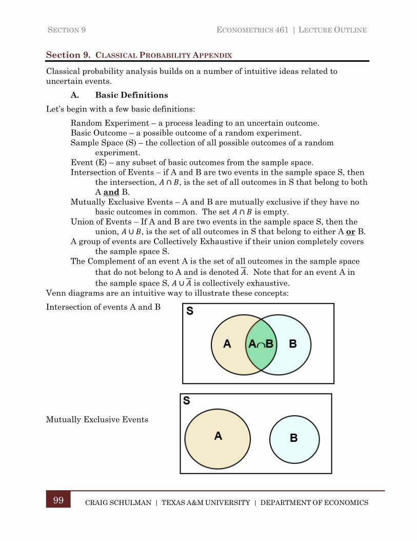
SECTION 9 ECONOMETRICS 461 | LECTURE OUTLINE
CRAIG SCHULMAN | TEXAS A&M UNIVERSITY | DEPARTMENT OF ECONOMICS
99
Section 9. CLASSICAL PROBABILITY APPENDIX
Classical probability analysis builds on a number of intuitive ideas related to uncertain events.
A. Basic Definitions
Let’s begin with a few basic definitions:
Random Experiment – a process leading to an uncertain outcome. Basic Outcome – a possible outcome of a random experiment. Sample Space (S) – the collection of all possible outcomes of a random
experiment. Event (E) – any subset of basic outcomes from the sample space. Intersection of Events – if A and B are two events in the sample space S, then
the intersection, ∩ , is the set of all outcomes in S that belong to both A and B.
Mutually Exclusive Events – A and B are mutually exclusive if they have no basic outcomes in common. The set ∩ is empty.
Union of Events – If A and B are two events in the sample space S, then the union, ∪ , is the set of all outcomes in S that belong to either A or B.
A group of events are Collectively Exhaustive if their union completely covers the sample space S.
The Complement of an event A is the set of all outcomes in the sample space that do not belong to A and is denoted . Note that for an event A in the sample space S, ∪ is collectively exhaustive.
Venn diagrams are an intuitive way to illustrate these concepts:
Intersection of events A and B
Mutually Exclusive Events
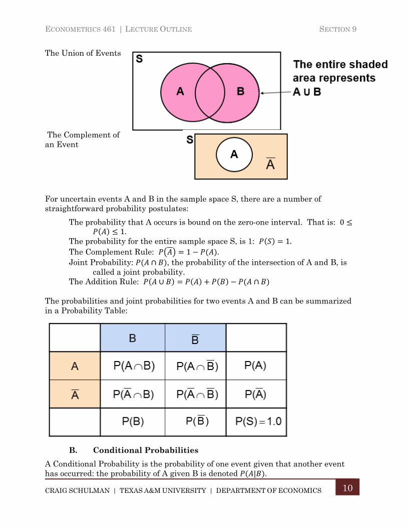
ECONOMETRICS 461 | LECTURE OUTLINE SECTION 9
CRAIG SCHULMAN | TEXAS A&M UNIVERSITY | DEPARTMENT OF ECONOMICS
10
The Union of Events
The Complement of an Event
For uncertain events A and B in the sample space S, there are a number of straightforward probability postulates:
The probability that A occurs is bound on the zero-one interval. That is: 01.
The probability for the entire sample space S, is 1: 1. The Complement Rule: 1 . Joint Probability: ∩ , the probability of the intersection of A and B, is
called a joint probability. The Addition Rule: ∪ ∩
The probabilities and joint probabilities for two events A and B can be summarized in a Probability Table:
B. Conditional Probabilities
A Conditional Probability is the probability of one event given that another event has occurred: the probability of A given B is denoted | .
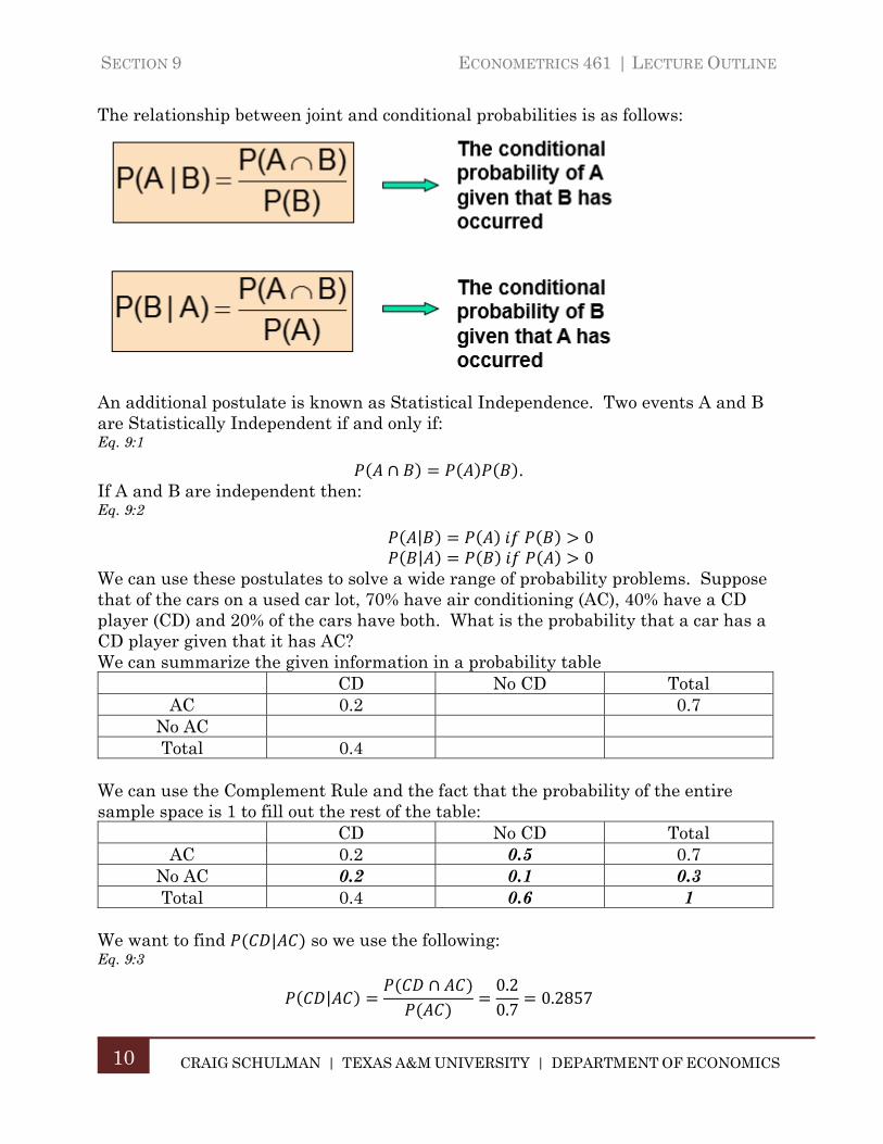
SECTION 9 ECONOMETRICS 461 | LECTURE OUTLINE
CRAIG SCHULMAN | TEXAS A&M UNIVERSITY | DEPARTMENT OF ECONOMICS
10
The relationship between joint and conditional probabilities is as follows:
An additional postulate is known as Statistical Independence. Two events A and B are Statistically Independent if and only if: Eq. 9:1
∩ . If A and B are independent then: Eq. 9:2
| 0 | 0
We can use these postulates to solve a wide range of probability problems. Suppose that of the cars on a used car lot, 70% have air conditioning (AC), 40% have a CD player (CD) and 20% of the cars have both. What is the probability that a car has a CD player given that it has AC? We can summarize the given information in a probability table
CD No CD Total AC 0.2 0.7
No AC Total 0.4
We can use the Complement Rule and the fact that the probability of the entire sample space is 1 to fill out the rest of the table:
CD No CD Total AC 0.2 0.5 0.7
No AC 0.2 0.1 0.3 Total 0.4 0.6 1
We want to find | so we use the following: Eq. 9:3
|∩ 0.2
0.70.2857
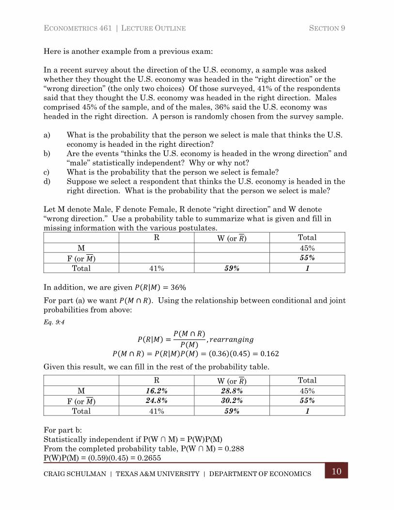
ECONOMETRICS 461 | LECTURE OUTLINE SECTION 9
CRAIG SCHULMAN | TEXAS A&M UNIVERSITY | DEPARTMENT OF ECONOMICS
10
Here is another example from a previous exam: In a recent survey about the direction of the U.S. economy, a sample was asked whether they thought the U.S. economy was headed in the “right direction” or the “wrong direction” (the only two choices) Of those surveyed, 41% of the respondents said that they thought the U.S. economy was headed in the right direction. Males comprised 45% of the sample, and of the males, 36% said the U.S. economy was headed in the right direction. A person is randomly chosen from the survey sample. a) What is the probability that the person we select is male that thinks the U.S.
economy is headed in the right direction? b) Are the events “thinks the U.S. economy is headed in the wrong direction” and
“male” statistically independent? Why or why not? c) What is the probability that the person we select is female? d) Suppose we select a respondent that thinks the U.S. economy is headed in the
right direction. What is the probability that the person we select is male? Let M denote Male, F denote Female, R denote “right direction” and W denote “wrong direction.” Use a probability table to summarize what is given and fill in missing information with the various postulates.
R W (or ) Total M 45%
F (or ) 55% Total 41% 59% 1
In addition, we are given | 36%
For part (a) we want ∩ . Using the relationship between conditional and joint probabilities from above:
Eq. 9:4
|∩
,
∩ | 0.36 0.45 0.162
Given this result, we can fill in the rest of the probability table.
R W (or ) Total M 16.2% 28.8% 45%
F (or ) 24.8% 30.2% 55% Total 41% 59% 1
For part b: Statistically independent if P(W ∩ M) = P(W)P(M) From the completed probability table, P(W ∩ M) = 0.288 P(W)P(M) = (0.59)(0.45) = 0.2655
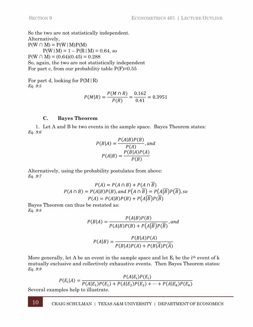
SECTION 9 ECONOMETRICS 461 | LECTURE OUTLINE
CRAIG SCHULMAN | TEXAS A&M UNIVERSITY | DEPARTMENT OF ECONOMICS
10
So the two are not statistically independent. Alternatively, P(W ∩ M) = P(W|M)P(M) P(W|M) = 1 – P(R|M) = 0.64, so P(W ∩ M) = (0.64)(0.45) = 0.288 So, again, the two are not statistically independent For part c, from our probability table P(F)=0.55 For part d, looking for P(M|R) Eq. 9:5
|∩ 0.162
0.410.3951
C. Bayes Theorem
1. Let A and B be two events in the sample space. Bayes Theorem states: Eq. 9:6
||
,
||
Alternatively, using the probability postulates from above: Eq. 9:7
∩ ∩ ∩ | , ∩ ,
| Bayes Theorem can thus be restated as: Eq. 9:8
||
|,
||
| |
More generally, let A be an event in the sample space and let Ei be the ith event of k mutually exclusive and collectively exhaustive events. Then Bayes Theorem states: Eq. 9:9
||
| | ⋯ |
Several examples help to illustrate.
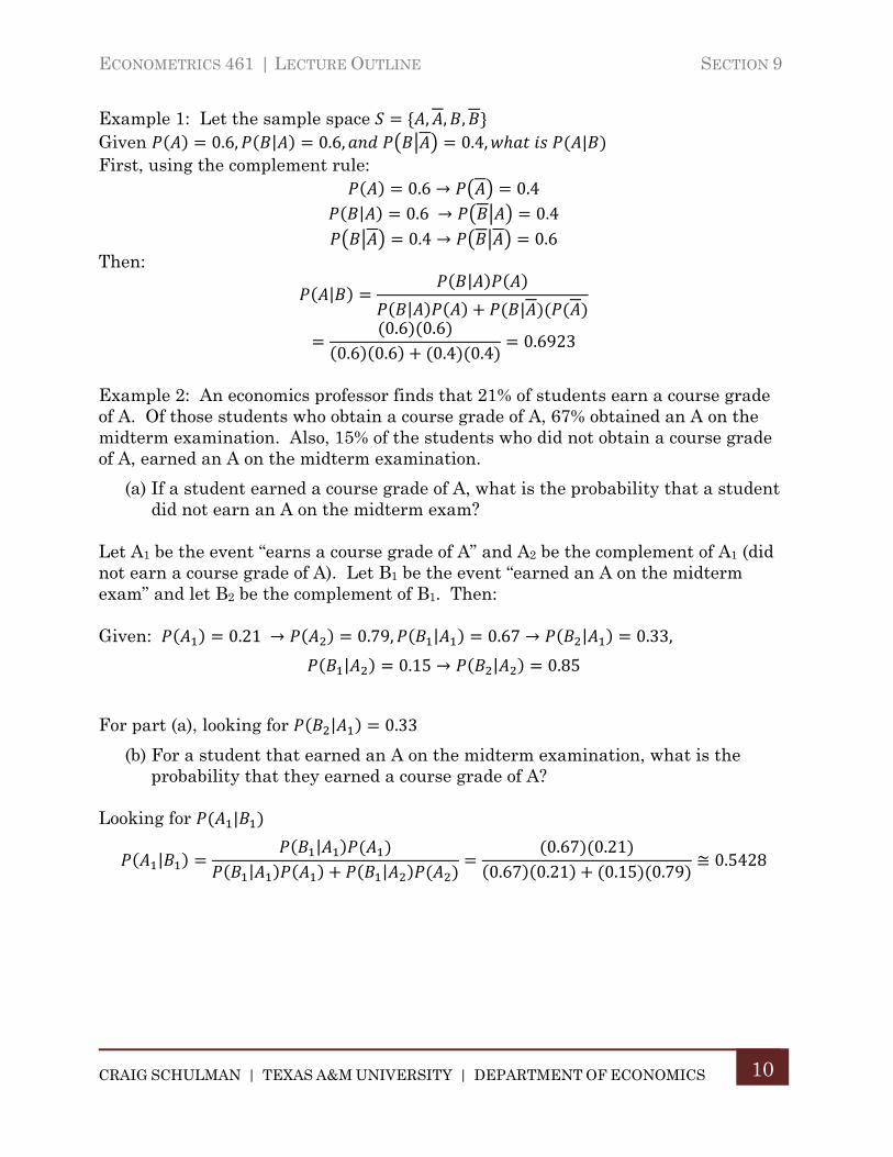
ECONOMETRICS 461 | LECTURE OUTLINE SECTION 9
CRAIG SCHULMAN | TEXAS A&M UNIVERSITY | DEPARTMENT OF ECONOMICS
10
Example 1: Let the sample space , , , Given 0.6, | 0.6, 0.4, | First, using the complement rule:
0.6 → 0.4| 0.6 → 0.4
0.4 → 0.6 Then:
||
| |
0.6 0.60.6 0.6 0.4 0.4
0.6923
Example 2: An economics professor finds that 21% of students earn a course grade of A. Of those students who obtain a course grade of A, 67% obtained an A on the midterm examination. Also, 15% of the students who did not obtain a course grade of A, earned an A on the midterm examination.
(a) If a student earned a course grade of A, what is the probability that a student did not earn an A on the midterm exam?
Let A1 be the event “earns a course grade of A” and A2 be the complement of A1 (did not earn a course grade of A). Let B1 be the event “earned an A on the midterm exam” and let B2 be the complement of B1. Then: Given: 0.21 → 0.79, | 0.67 → | 0.33,
| 0.15 → | 0.85
For part (a), looking for | 0.33
(b) For a student that earned an A on the midterm examination, what is the probability that they earned a course grade of A?
Looking for |
||
| |0.67 0.21
0.67 0.21 0.15 0.79≅ 0.5428

SECTION 10 ECONOMETRICS 461 | LECTURE OUTLINE
CRAIG SCHULMAN | TEXAS A&M UNIVERSITY | DEPARTMENT OF ECONOMICS
10
Section 10. MICROSOFT EXCEL APPENDIX
A. Excel Basics
In progress …
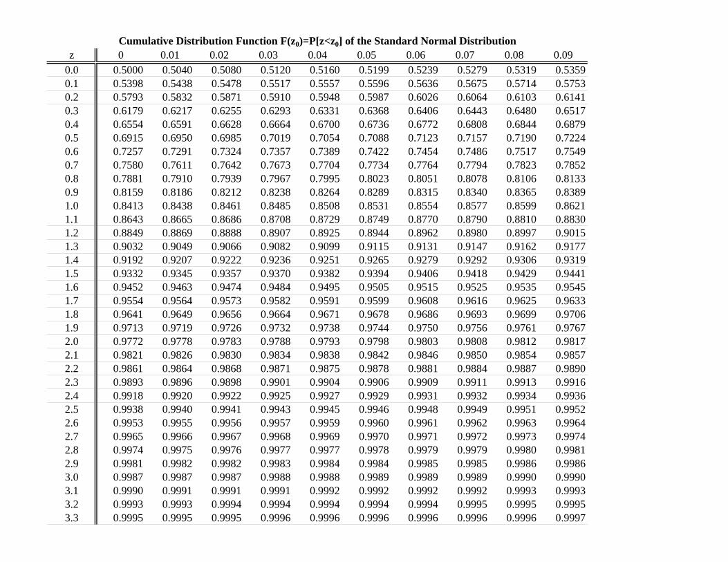
Cumulative Distribution Function F(z0)=P[z<z0] of the Standard Normal Distributionz 0 0.01 0.02 0.03 0.04 0.05 0.06 0.07 0.08 0.09
0.0 0.5000 0.5040 0.5080 0.5120 0.5160 0.5199 0.5239 0.5279 0.5319 0.53590.1 0.5398 0.5438 0.5478 0.5517 0.5557 0.5596 0.5636 0.5675 0.5714 0.57530.2 0.5793 0.5832 0.5871 0.5910 0.5948 0.5987 0.6026 0.6064 0.6103 0.61410.3 0.6179 0.6217 0.6255 0.6293 0.6331 0.6368 0.6406 0.6443 0.6480 0.65170.4 0.6554 0.6591 0.6628 0.6664 0.6700 0.6736 0.6772 0.6808 0.6844 0.68790.5 0.6915 0.6950 0.6985 0.7019 0.7054 0.7088 0.7123 0.7157 0.7190 0.72240.6 0.7257 0.7291 0.7324 0.7357 0.7389 0.7422 0.7454 0.7486 0.7517 0.75490.7 0.7580 0.7611 0.7642 0.7673 0.7704 0.7734 0.7764 0.7794 0.7823 0.78520.8 0.7881 0.7910 0.7939 0.7967 0.7995 0.8023 0.8051 0.8078 0.8106 0.81330.9 0.8159 0.8186 0.8212 0.8238 0.8264 0.8289 0.8315 0.8340 0.8365 0.83891.0 0.8413 0.8438 0.8461 0.8485 0.8508 0.8531 0.8554 0.8577 0.8599 0.86211.1 0.8643 0.8665 0.8686 0.8708 0.8729 0.8749 0.8770 0.8790 0.8810 0.88301.2 0.8849 0.8869 0.8888 0.8907 0.8925 0.8944 0.8962 0.8980 0.8997 0.90151.3 0.9032 0.9049 0.9066 0.9082 0.9099 0.9115 0.9131 0.9147 0.9162 0.91771.4 0.9192 0.9207 0.9222 0.9236 0.9251 0.9265 0.9279 0.9292 0.9306 0.93191.5 0.9332 0.9345 0.9357 0.9370 0.9382 0.9394 0.9406 0.9418 0.9429 0.94411.6 0.9452 0.9463 0.9474 0.9484 0.9495 0.9505 0.9515 0.9525 0.9535 0.95451.7 0.9554 0.9564 0.9573 0.9582 0.9591 0.9599 0.9608 0.9616 0.9625 0.96331.8 0.9641 0.9649 0.9656 0.9664 0.9671 0.9678 0.9686 0.9693 0.9699 0.97061.9 0.9713 0.9719 0.9726 0.9732 0.9738 0.9744 0.9750 0.9756 0.9761 0.97672.0 0.9772 0.9778 0.9783 0.9788 0.9793 0.9798 0.9803 0.9808 0.9812 0.98172.1 0.9821 0.9826 0.9830 0.9834 0.9838 0.9842 0.9846 0.9850 0.9854 0.98572.2 0.9861 0.9864 0.9868 0.9871 0.9875 0.9878 0.9881 0.9884 0.9887 0.98902.3 0.9893 0.9896 0.9898 0.9901 0.9904 0.9906 0.9909 0.9911 0.9913 0.99162.4 0.9918 0.9920 0.9922 0.9925 0.9927 0.9929 0.9931 0.9932 0.9934 0.99362.5 0.9938 0.9940 0.9941 0.9943 0.9945 0.9946 0.9948 0.9949 0.9951 0.99522.6 0.9953 0.9955 0.9956 0.9957 0.9959 0.9960 0.9961 0.9962 0.9963 0.99642.7 0.9965 0.9966 0.9967 0.9968 0.9969 0.9970 0.9971 0.9972 0.9973 0.99742.8 0.9974 0.9975 0.9976 0.9977 0.9977 0.9978 0.9979 0.9979 0.9980 0.99812.9 0.9981 0.9982 0.9982 0.9983 0.9984 0.9984 0.9985 0.9985 0.9986 0.99863.0 0.9987 0.9987 0.9987 0.9988 0.9988 0.9989 0.9989 0.9989 0.9990 0.99903.1 0.9990 0.9991 0.9991 0.9991 0.9992 0.9992 0.9992 0.9992 0.9993 0.99933.2 0.9993 0.9993 0.9994 0.9994 0.9994 0.9994 0.9994 0.9995 0.9995 0.99953.3 0.9995 0.9995 0.9995 0.9996 0.9996 0.9996 0.9996 0.9996 0.9996 0.9997
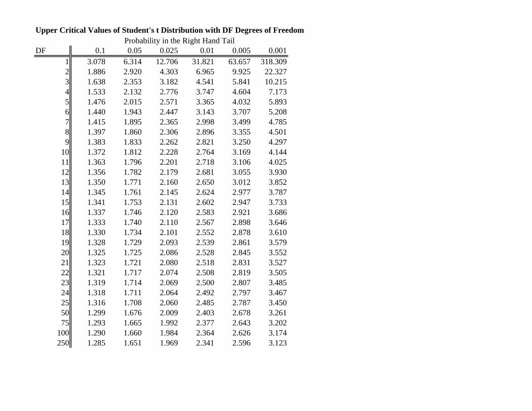
Upper Critical Values of Student's t Distribution with DF Degrees of FreedomProbability in the Right Hand Tail
DF 0.1 0.05 0.025 0.01 0.005 0.0011 3.078 6.314 12.706 31.821 63.657 318.3092 1.886 2.920 4.303 6.965 9.925 22.3273 1.638 2.353 3.182 4.541 5.841 10.2154 1.533 2.132 2.776 3.747 4.604 7.1735 1.476 2.015 2.571 3.365 4.032 5.8936 1.440 1.943 2.447 3.143 3.707 5.2087 1.415 1.895 2.365 2.998 3.499 4.7858 1.397 1.860 2.306 2.896 3.355 4.5019 1.383 1.833 2.262 2.821 3.250 4.297
10 1.372 1.812 2.228 2.764 3.169 4.14411 1.363 1.796 2.201 2.718 3.106 4.02512 1.356 1.782 2.179 2.681 3.055 3.93013 1.350 1.771 2.160 2.650 3.012 3.85214 1.345 1.761 2.145 2.624 2.977 3.78715 1.341 1.753 2.131 2.602 2.947 3.73316 1.337 1.746 2.120 2.583 2.921 3.68617 1.333 1.740 2.110 2.567 2.898 3.64618 1.330 1.734 2.101 2.552 2.878 3.61019 1.328 1.729 2.093 2.539 2.861 3.57920 1.325 1.725 2.086 2.528 2.845 3.55221 1.323 1.721 2.080 2.518 2.831 3.52722 1.321 1.717 2.074 2.508 2.819 3.50523 1.319 1.714 2.069 2.500 2.807 3.48524 1.318 1.711 2.064 2.492 2.797 3.46725 1.316 1.708 2.060 2.485 2.787 3.45050 1.299 1.676 2.009 2.403 2.678 3.26175 1.293 1.665 1.992 2.377 2.643 3.202
100 1.290 1.660 1.984 2.364 2.626 3.174250 1.285 1.651 1.969 2.341 2.596 3.123
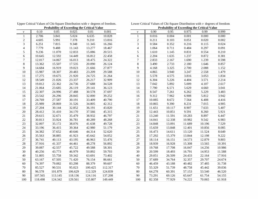
Upper Critical Values of Chi-Square Distribution with v degrees of freedom. Lower Critical Values of Chi-Square Distribution with v degrees of freedom.Probability of Exceeding the Critical Value Probability of Exceeding the Critical Value
v 0.10 0.05 0.025 0.01 0.001 v 0.90 0.95 0.975 0.99 0.9991 2.706 3.841 5.024 6.635 10.828 1 0.016 0.004 0.001 0.000 0.0002 4.605 5.991 7.378 9.210 13.816 2 0.211 0.103 0.051 0.020 0.0023 6.251 7.815 9.348 11.345 16.266 3 0.584 0.352 0.216 0.115 0.0244 7.779 9.488 11.143 13.277 18.467 4 1.064 0.711 0.484 0.297 0.0915 9.236 11.070 12.833 15.086 20.515 5 1.610 1.145 0.831 0.554 0.2106 10.645 12.592 14.449 16.812 22.458 6 2.204 1.635 1.237 0.872 0.3817 12.017 14.067 16.013 18.475 24.322 7 2.833 2.167 1.690 1.239 0.5988 13.362 15.507 17.535 20.090 26.124 8 3.490 2.733 2.180 1.646 0.8579 14.684 16.919 19.023 21.666 27.877 9 4.168 3.325 2.700 2.088 1.15210 15.987 18.307 20.483 23.209 29.588 10 4.865 3.940 3.247 2.558 1.47911 17.275 19.675 21.920 24.725 31.264 11 5.578 4.575 3.816 3.053 1.83412 18.549 21.026 23.337 26.217 32.909 12 6.304 5.226 4.404 3.571 2.21413 19.812 22.362 24.736 27.688 34.528 13 7.042 5.892 5.009 4.107 2.61714 21.064 23.685 26.119 29.141 36.123 14 7.790 6.571 5.629 4.660 3.04115 22.307 24.996 27.488 30.578 37.697 15 8.547 7.261 6.262 5.229 3.48316 23.542 26.296 28.845 32.000 39.252 16 9.312 7.962 6.908 5.812 3.94217 24.769 27.587 30.191 33.409 40.790 17 10.085 8.672 7.564 6.408 4.41618 25.989 28.869 31.526 34.805 42.312 18 10.865 9.390 8.231 7.015 4.90519 27.204 30.144 32.852 36.191 43.820 19 11.651 10.117 8.907 7.633 5.40720 28.412 31.410 34.170 37.566 45.315 20 12.443 10.851 9.591 8.260 5.92121 29.615 32.671 35.479 38.932 46.797 21 13.240 11.591 10.283 8.897 6.44722 30.813 33.924 36.781 40.289 48.268 22 14.041 12.338 10.982 9.542 6.98323 32.007 35.172 38.076 41.638 49.728 23 14.848 13.091 11.689 10.196 7.52924 33.196 36.415 39.364 42.980 51.179 24 15.659 13.848 12.401 10.856 8.08525 34.382 37.652 40.646 44.314 52.620 25 16.473 14.611 13.120 11.524 8.64926 35.563 38.885 41.923 45.642 54.052 26 17.292 15.379 13.844 12.198 9.22227 36.741 40.113 43.195 46.963 55.476 27 18.114 16.151 14.573 12.879 9.80328 37.916 41.337 44.461 48.278 56.892 28 18.939 16.928 15.308 13.565 10.39129 39.087 42.557 45.722 49.588 58.301 29 19.768 17.708 16.047 14.256 10.98630 40.256 43.773 46.979 50.892 59.703 30 20.599 18.493 16.791 14.953 11.58840 51.805 55.758 59.342 63.691 73.402 40 29.051 26.509 24.433 22.164 17.91650 63.167 67.505 71.420 76.154 86.661 50 37.689 34.764 32.357 29.707 24.67460 74.397 79.082 83.298 88.379 99.607 60 46.459 43.188 40.482 37.485 31.73870 85.527 90.531 95.023 100.425 112.317 70 55.329 51.739 48.758 45.442 39.03680 96.578 101.879 106.629 112.329 124.839 80 64.278 60.391 57.153 53.540 46.52090 107.565 113.145 118.136 124.116 137.208 90 73.291 69.126 65.647 61.754 54.155100 118.498 124.342 129.561 135.807 149.449 100 82.358 77.929 74.222 70.065 61.918
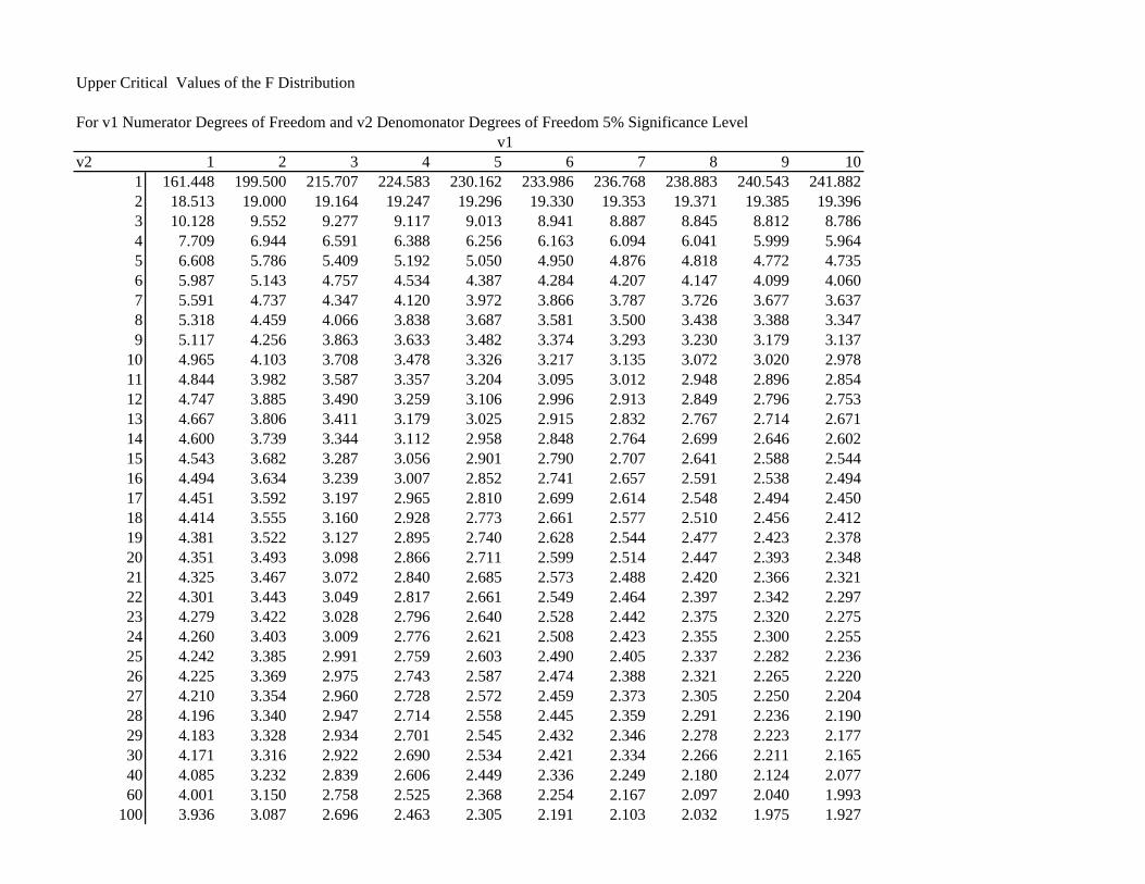
Upper Critical Values of the F Distribution
For v1 Numerator Degrees of Freedom and v2 Denomonator Degrees of Freedom 5% Significance Levelv1
v2 1 2 3 4 5 6 7 8 9 101 161.448 199.500 215.707 224.583 230.162 233.986 236.768 238.883 240.543 241.8822 18.513 19.000 19.164 19.247 19.296 19.330 19.353 19.371 19.385 19.3963 10.128 9.552 9.277 9.117 9.013 8.941 8.887 8.845 8.812 8.7864 7.709 6.944 6.591 6.388 6.256 6.163 6.094 6.041 5.999 5.9645 6.608 5.786 5.409 5.192 5.050 4.950 4.876 4.818 4.772 4.7356 5.987 5.143 4.757 4.534 4.387 4.284 4.207 4.147 4.099 4.0607 5.591 4.737 4.347 4.120 3.972 3.866 3.787 3.726 3.677 3.6378 5.318 4.459 4.066 3.838 3.687 3.581 3.500 3.438 3.388 3.3479 5.117 4.256 3.863 3.633 3.482 3.374 3.293 3.230 3.179 3.137
10 4.965 4.103 3.708 3.478 3.326 3.217 3.135 3.072 3.020 2.97811 4.844 3.982 3.587 3.357 3.204 3.095 3.012 2.948 2.896 2.85412 4.747 3.885 3.490 3.259 3.106 2.996 2.913 2.849 2.796 2.75313 4.667 3.806 3.411 3.179 3.025 2.915 2.832 2.767 2.714 2.67114 4.600 3.739 3.344 3.112 2.958 2.848 2.764 2.699 2.646 2.60215 4.543 3.682 3.287 3.056 2.901 2.790 2.707 2.641 2.588 2.54416 4.494 3.634 3.239 3.007 2.852 2.741 2.657 2.591 2.538 2.49417 4.451 3.592 3.197 2.965 2.810 2.699 2.614 2.548 2.494 2.45018 4.414 3.555 3.160 2.928 2.773 2.661 2.577 2.510 2.456 2.41219 4.381 3.522 3.127 2.895 2.740 2.628 2.544 2.477 2.423 2.37820 4.351 3.493 3.098 2.866 2.711 2.599 2.514 2.447 2.393 2.34821 4.325 3.467 3.072 2.840 2.685 2.573 2.488 2.420 2.366 2.32122 4.301 3.443 3.049 2.817 2.661 2.549 2.464 2.397 2.342 2.29723 4.279 3.422 3.028 2.796 2.640 2.528 2.442 2.375 2.320 2.27524 4.260 3.403 3.009 2.776 2.621 2.508 2.423 2.355 2.300 2.25525 4.242 3.385 2.991 2.759 2.603 2.490 2.405 2.337 2.282 2.23626 4.225 3.369 2.975 2.743 2.587 2.474 2.388 2.321 2.265 2.22027 4.210 3.354 2.960 2.728 2.572 2.459 2.373 2.305 2.250 2.20428 4.196 3.340 2.947 2.714 2.558 2.445 2.359 2.291 2.236 2.19029 4.183 3.328 2.934 2.701 2.545 2.432 2.346 2.278 2.223 2.17730 4.171 3.316 2.922 2.690 2.534 2.421 2.334 2.266 2.211 2.16540 4.085 3.232 2.839 2.606 2.449 2.336 2.249 2.180 2.124 2.07760 4.001 3.150 2.758 2.525 2.368 2.254 2.167 2.097 2.040 1.993
100 3.936 3.087 2.696 2.463 2.305 2.191 2.103 2.032 1.975 1.927