Embed Size (px)
Citation preview
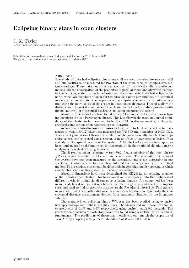
Mon. Not. R. Astron. Soc. 000, 000–000 (0000) Printed 11 April 2006 (MN LATEX style file v2.2)
Eclipsing binary stars in open clusters
J. K. TaylorDepartment of Chemistry and Physics, Keele University, Staffordshire, ST5 5BG, UK
Submitted for postgraduate research degree qualification on 3rd February 2005This is not the version which was accepted on 1st March 2006
ABSTRACTThe study of detached eclipsing binary stars allows accurate absolute masses, radiiand luminosities to be measured for two stars of the same chemical composition, dis-tance and age. These data can provide a good test of theoretical stellar evolutionarymodels, aid the investigation of the properties of peculiar stars, and allow the distanceto the eclipsing system to be found using empirical methods. Detached eclipsing bi-naries which are members of open clusters provide a more powerful test of theoreticalmodels, which must match the properties of the eclipsing system whilst simultaneouslypredicting the morphology of the cluster in photometric diagrams. They also allow thedistance and the metal abundance of the cluster to be found, avoiding problems withfitting empirical or theoretical isochrones in colour-magnitude diagrams.
Absolute dimensions have been found for V615Per and V618Per, which are eclips-ing members of the hPersei open cluster. This has allowed the fractional metal abun-dance of the cluster to be measured to be Z ≈ 0.01, in disagreement with the solarchemical composition often assumed in the literature.
Accurate absolute dimensions (masses to 1.4%, radii to 1.1% and effective temper-atures to within 800K) have been measured for V453 Cygni, a member of NGC 6871.The current generation of theoretical stellar models can successfully match these prop-erties, as well as the central concentration of mass of the primary star as derived froma study of the apsidal motion of the system. A Monte Carlo analysis technique hasbeen implemented to determine robust uncertainties in the results of the photometricanalysis of detached eclipsing binaries.
The B-type subgiant eclipsing system V621 Per, a member of the open clusterχPersei, which is related to h Persei, has been studied. The absolute dimensions ofthe system have not been measured as the secondary star is not detectable in ourspectroscopic observations, but have been inferred from a comparison with theoreticalmodels. The secondary star should be detectable in very high-quality spectra, in whichcase further study of this system will be very rewarding.
Absolute dimensions have been determined for HD 23642, an eclipsing memberof the Pleiades open cluster. This has allowed an investigation into the usefulness ofdifferent methods to find the distances to eclipsing binaries. A new method has beenintroduced, based on calibrations between surface brightness and effective tempera-ture, and used to find an accurate distance to the Pleiades of 139± 4 pc. This value isin good agreement with other distance measurements but does not agree with the con-troversial distance measurement derived from parallaxes obtained by the Hipparcossatellite.
The metallic-lined eclipsing binary WWAur has been studied using extensivenew spectroscopy and published light curves. The masses and radii have been found,to accuracies of 0.4% and 0.6% respectively, using entirely empirical methods. Theeffective temperatures of both stars have been found using a method which is almostfundamental. The predictions of theoretical models can only match the properties ofWWAur by adopting a large metal abundance of Z = 0.060± 0.005.
c© 0000 RAS
2 J. K. Taylor
1 Stellar properties . . . . . . . . . . . . . . . . . . . . . . . . . . . . . . . . . . . . . . . . . . . . . . . . . . . 3
1.1 Spectral classification . . . . . . . . . . . . . . . . . . . . . . . . . . . . . . . . . . . . . . . . . . . . . 3
1.2 Brightness and distance . . . . . . . . . . . . . . . . . . . . . . . . . . . . . . . . . . . . . . . . . . . 3
1.2.1 Interstellar extinction . . . . . . . . . . . . . . . . . . . . . . . . . . . . . . . . . . . . . . . . . . . 4
1.3 Stellar characteristics . . . . . . . . . . . . . . . . . . . . . . . . . . . . . . . . . . . . . . . . . . . . . 5
1.3.1 Stellar interferometry . . . . . . . . . . . . . . . . . . . . . . . . . . . . . . . . . . . . . . . . . . . 5
1.3.2 The effective temperature scale . . . . . . . . . . . . . . . . . . . . . . . . . . . . . . . . . .5
1.3.3 Teff s and angular diameters from the IRFM . . . . . . . . . . . . . . . . . . . . . 6
1.3.4 Stellar chemical compositions . . . . . . . . . . . . . . . . . . . . . . . . . . . . . . . . . . . 6
1.3.5 Bolometric corrections . . . . . . . . . . . . . . . . . . . . . . . . . . . . . . . . . . . . . . . . . . 7
1.3.6 Surface brightness relations . . . . . . . . . . . . . . . . . . . . . . . . . . . . . . . . . . . . . 7
1.4 Limb darkening . . . . . . . . . . . . . . . . . . . . . . . . . . . . . . . . . . . . . . . . . . . . . . . . . . . 9
1.4.1 Limb darkening laws . . . . . . . . . . . . . . . . . . . . . . . . . . . . . . . . . . . . . . . . . . . 10
1.4.2 Limb darkening and eclipsing binaries . . . . . . . . . . . . . . . . . . . . . . . . . . 11
1.5 Gravity darkening . . . . . . . . . . . . . . . . . . . . . . . . . . . . . . . . . . . . . . . . . . . . . . . 11
2 Stellar evolution . . . . . . . . . . . . . . . . . . . . . . . . . . . . . . . . . . . . . . . . . . . . . . . . . . . 12
2.1 The evolution of single stars . . . . . . . . . . . . . . . . . . . . . . . . . . . . . . . . . . . . . 12
2.1.1 The formation of stars . . . . . . . . . . . . . . . . . . . . . . . . . . . . . . . . . . . . . . . . . 12
2.1.2 Main sequence evolution . . . . . . . . . . . . . . . . . . . . . . . . . . . . . . . . . . . . . . . 13
2.1.3 The evolution of low-mass stars . . . . . . . . . . . . . . . . . . . . . . . . . . . . . . . . 13
2.1.4 The evolution of intermediate-mass stars . . . . . . . . . . . . . . . . . . . . . . . 13
2.1.5 The evolution of massive stars . . . . . . . . . . . . . . . . . . . . . . . . . . . . . . . . . 14
3 Modelling of stars . . . . . . . . . . . . . . . . . . . . . . . . . . . . . . . . . . . . . . . . . . . . . . . . . 14
3.1 Physical phenomena in models . . . . . . . . . . . . . . . . . . . . . . . . . . . . . . . . . . . 14
3.1.1 Equation of state . . . . . . . . . . . . . . . . . . . . . . . . . . . . . . . . . . . . . . . . . . . . . . 14
3.1.2 Opacity . . . . . . . . . . . . . . . . . . . . . . . . . . . . . . . . . . . . . . . . . . . . . . . . . . . . . . . . 14
3.1.3 Energy transport . . . . . . . . . . . . . . . . . . . . . . . . . . . . . . . . . . . . . . . . . . . . . . .14
3.1.4 Convective core overshooting . . . . . . . . . . . . . . . . . . . . . . . . . . . . . . . . . . . 15
3.1.5 Convective efficiency . . . . . . . . . . . . . . . . . . . . . . . . . . . . . . . . . . . . . . . . . . . 16
3.1.6 The effect of stellar rotation . . . . . . . . . . . . . . . . . . . . . . . . . . . . . . . . . . . 16
3.1.7 The effect of mass loss . . . . . . . . . . . . . . . . . . . . . . . . . . . . . . . . . . . . . . . . . 16
3.1.8 The effect of diffusion . . . . . . . . . . . . . . . . . . . . . . . . . . . . . . . . . . . . . . . . . . 17
3.1.9 The effect of magnetic fields. . . . . . . . . . . . . . . . . . . . . . . . . . . . . . . . . . . .17
3.2 Available theoretical stellar models . . . . . . . . . . . . . . . . . . . . . . . . . . . . . . 17
3.2.1 Hejlesen theoretical models. . . . . . . . . . . . . . . . . . . . . . . . . . . . . . . . . . . . .17
3.2.2 Granada theoretical models . . . . . . . . . . . . . . . . . . . . . . . . . . . . . . . . . . . . 17
3.2.3 Geneva theoretical models. . . . . . . . . . . . . . . . . . . . . . . . . . . . . . . . . . . . . .17
3.2.4 Padova theoretical models . . . . . . . . . . . . . . . . . . . . . . . . . . . . . . . . . . . . . .17
3.2.5 Cambridge theoretical models . . . . . . . . . . . . . . . . . . . . . . . . . . . . . . . . . . 17
3.2.6 Other theoretical models . . . . . . . . . . . . . . . . . . . . . . . . . . . . . . . . . . . . . . . 18
3.3 Comments on stellar models . . . . . . . . . . . . . . . . . . . . . . . . . . . . . . . . . . . . . 18
4 Spectral characteristics of stars . . . . . . . . . . . . . . . . . . . . . . . . . . . . . . . . . . . . 18
4.1 Spectral lines . . . . . . . . . . . . . . . . . . . . . . . . . . . . . . . . . . . . . . . . . . . . . . . . . . . . 18
4.1.1 Spectral line broadening . . . . . . . . . . . . . . . . . . . . . . . . . . . . . . . . . . . . . . . 19
4.2 Spectral features in stars. . . . . . . . . . . . . . . . . . . . . . . . . . . . . . . . . . . . . . . . .20
4.3 Stellar model atmospheres . . . . . . . . . . . . . . . . . . . . . . . . . . . . . . . . . . . . . . . 20
4.3.1 The current status of model atmospheres . . . . . . . . . . . . . . . . . . . . . . . 20
4.3.2 Convection in model atmospheres . . . . . . . . . . . . . . . . . . . . . . . . . . . . . . 21
4.3.3 The future of stellar model atmospheres . . . . . . . . . . . . . . . . . . . . . . . . 21
4.4 Calculation of theoretical stellar spectra . . . . . . . . . . . . . . . . . . . . . . . . . 21
4.4.1 Microturbulence velocity . . . . . . . . . . . . . . . . . . . . . . . . . . . . . . . . . . . . . . . 21
4.4.2 The uclsyn spectral synthesis code . . . . . . . . . . . . . . . . . . . . . . . . . . . . . 22
4.4.3 Abundance analysis of stellar spectra. . . . . . . . . . . . . . . . . . . . . . . . . . .22
4.5 Spectral peculiarity in stars . . . . . . . . . . . . . . . . . . . . . . . . . . . . . . . . . . . . . . 22
4.5.1 Metallic-lined stars. . . . . . . . . . . . . . . . . . . . . . . . . . . . . . . . . . . . . . . . . . . . .22
4.5.2 Chemically peculiar stars . . . . . . . . . . . . . . . . . . . . . . . . . . . . . . . . . . . . . . 23
5 Multiple stars . . . . . . . . . . . . . . . . . . . . . . . . . . . . . . . . . . . . . . . . . . . . . . . . . . . . . 23
5.1 Dynamical characteristics of multiple stars . . . . . . . . . . . . . . . . . . . . . . . 23
5.2 Binary star systems . . . . . . . . . . . . . . . . . . . . . . . . . . . . . . . . . . . . . . . . . . . . . . 24
5.3 Eclipsing binary star systems . . . . . . . . . . . . . . . . . . . . . . . . . . . . . . . . . . . . 25
6 Detached eclipsing binary star systems. . . . . . . . . . . . . . . . . . . . . . . . . . . . .26
6.1 Comparison with theoretical stellar models. . . . . . . . . . . . . . . . . . . . . . .28
6.1.1 The methods of comparison . . . . . . . . . . . . . . . . . . . . . . . . . . . . . . . . . . . . 28
6.1.2 Further work . . . . . . . . . . . . . . . . . . . . . . . . . . . . . . . . . . . . . . . . . . . . . . . . . . . 29
6.1.3 The difference between binary and single stars . . . . . . . . . . . . . . . . . 30
6.2 Metal and helium abundances of nearby stars . . . . . . . . . . . . . . . . . . . . 30
6.3 Detached eclipsing binaries as standard candles . . . . . . . . . . . . . . . . . . 31
6.3.1 Distances from bolometric corrections . . . . . . . . . . . . . . . . . . . . . . . . . . 31
6.3.2 Distances from surface brightness relations . . . . . . . . . . . . . . . . . . . . . 32
6.3.3 Distances from modelling of stellar SEDs . . . . . . . . . . . . . . . . . . . . . . . 32
6.3.4 Recent results for the distance to eclipsing binaries . . . . . . . . . . . . .32
6.4 Detached eclipsing binaries in stellar systems . . . . . . . . . . . . . . . . . . . . 33
6.4.1 Literature results on dEBs in open clusters . . . . . . . . . . . . . . . . . . . . . 33
7 Tidal effects . . . . . . . . . . . . . . . . . . . . . . . . . . . . . . . . . . . . . . . . . . . . . . . . . . . . . . . 34
7.1 Orbital circularization and rotational synchronism . . . . . . . . . . . . . . . 34
7.1.1 The theory of Zahn . . . . . . . . . . . . . . . . . . . . . . . . . . . . . . . . . . . . . . . . . . . . 34
7.1.2 The theory of Tassoul & Tassoul . . . . . . . . . . . . . . . . . . . . . . . . . . . . . . . 35
7.1.3 The theory of Press, Wiita & Smarr . . . . . . . . . . . . . . . . . . . . . . . . . . . . 35
7.1.4 The theory of Hut. . . . . . . . . . . . . . . . . . . . . . . . . . . . . . . . . . . . . . . . . . . . . .35
7.1.5 Comparison with observations . . . . . . . . . . . . . . . . . . . . . . . . . . . . . . . . . .35
7.1.6 Summary . . . . . . . . . . . . . . . . . . . . . . . . . . . . . . . . . . . . . . . . . . . . . . . . . . . . . . 36
7.2 Apsidal motion . . . . . . . . . . . . . . . . . . . . . . . . . . . . . . . . . . . . . . . . . . . . . . . . . . 37
7.2.1 Relativistic apsidal motion . . . . . . . . . . . . . . . . . . . . . . . . . . . . . . . . . . . . . 37
7.2.2 Comparison with theoretical models . . . . . . . . . . . . . . . . . . . . . . . . . . . . 38
7.2.3 Comparison between observations and theory . . . . . . . . . . . . . . . . . . 38
8 Open clusters . . . . . . . . . . . . . . . . . . . . . . . . . . . . . . . . . . . . . . . . . . . . . . . . . . . . . . 38
8.1 Photometric characteristics of open clusters . . . . . . . . . . . . . . . . . . . . . . 39
8.2 Colour-magnitude diagrams of open clusters . . . . . . . . . . . . . . . . . . . . . 40
8.3 Dynamical characteristics of open clusters. . . . . . . . . . . . . . . . . . . . . . . .42
9 The galactic and extragalactic distance scale . . . . . . . . . . . . . . . . . . . . . . .42
9.1 Parallax-based distances to stars . . . . . . . . . . . . . . . . . . . . . . . . . . . . . . . . . 42
9.1.1 Trigonometrical parallax . . . . . . . . . . . . . . . . . . . . . . . . . . . . . . . . . . . . . . . 42
9.1.2 Spectroscopic and photometric parallax . . . . . . . . . . . . . . . . . . . . . . . . 43
9.2 Distances to binary stars. . . . . . . . . . . . . . . . . . . . . . . . . . . . . . . . . . . . . . . . .43
9.2.1 Visual binaries . . . . . . . . . . . . . . . . . . . . . . . . . . . . . . . . . . . . . . . . . . . . . . . . . 43
9.2.2 Eclipsing binaries . . . . . . . . . . . . . . . . . . . . . . . . . . . . . . . . . . . . . . . . . . . . . . 43
9.3 Variable stars as standard candles . . . . . . . . . . . . . . . . . . . . . . . . . . . . . . . 43
9.3.1 δ Cepheid variables . . . . . . . . . . . . . . . . . . . . . . . . . . . . . . . . . . . . . . . . . . . . . 43
9.3.2 RRLyrae variables . . . . . . . . . . . . . . . . . . . . . . . . . . . . . . . . . . . . . . . . . . . . . 43
9.3.3 Type Ia supernovae. . . . . . . . . . . . . . . . . . . . . . . . . . . . . . . . . . . . . . . . . . . . .44
9.4 Distances to stellar clusters . . . . . . . . . . . . . . . . . . . . . . . . . . . . . . . . . . . . . . 44
9.5 The Galactic and extragalactic distance scale . . . . . . . . . . . . . . . . . . . . 44
10 Obtaining and reducing astronomical data . . . . . . . . . . . . . . . . . . . . . . . . 45
10.1 Telescopes . . . . . . . . . . . . . . . . . . . . . . . . . . . . . . . . . . . . . . . . . . . . . . . . . . . . . . 45
10.1.1 Optical aberration . . . . . . . . . . . . . . . . . . . . . . . . . . . . . . . . . . . . . . . . . . . . 45
10.2 Charge-coupled devices . . . . . . . . . . . . . . . . . . . . . . . . . . . . . . . . . . . . . . . . . 45
10.2.1 Advantages and disadvantages of CCDs . . . . . . . . . . . . . . . . . . . . . . . 46
10.2.2 Reduction of CCD data . . . . . . . . . . . . . . . . . . . . . . . . . . . . . . . . . . . . . . . 46
10.2.3 Debiassing CCD images . . . . . . . . . . . . . . . . . . . . . . . . . . . . . . . . . . . . . . . 46
10.2.4 Flat-fielding CCD images . . . . . . . . . . . . . . . . . . . . . . . . . . . . . . . . . . . . . 47
10.2.5 Photometry from CCD images . . . . . . . . . . . . . . . . . . . . . . . . . . . . . . . . 47
10.2.6 Aperture photometry . . . . . . . . . . . . . . . . . . . . . . . . . . . . . . . . . . . . . . . . . 47
10.2.7 Point spread function photometry . . . . . . . . . . . . . . . . . . . . . . . . . . . . . 48
10.2.8 Optimal photometry . . . . . . . . . . . . . . . . . . . . . . . . . . . . . . . . . . . . . . . . . . 48
10.3 Grating spectrographs . . . . . . . . . . . . . . . . . . . . . . . . . . . . . . . . . . . . . . . . . . 48
10.3.1 Reduction of CCD grating spectra . . . . . . . . . . . . . . . . . . . . . . . . . . . . 48
10.4 Echelle spectrographs . . . . . . . . . . . . . . . . . . . . . . . . . . . . . . . . . . . . . . . . . . . 49
10.5 Observational procedures for the study of dEBs . . . . . . . . . . . . . . . . . 49
10.5.1 CCD photometry . . . . . . . . . . . . . . . . . . . . . . . . . . . . . . . . . . . . . . . . . . . . . 49
10.5.2 Grating spectroscopy. . . . . . . . . . . . . . . . . . . . . . . . . . . . . . . . . . . . . . . . . .49
11 Determination of spectroscopic orbits . . . . . . . . . . . . . . . . . . . . . . . . . . . . . 50
11.1 The equations of spectroscopic orbits . . . . . . . . . . . . . . . . . . . . . . . . . . . 50
11.2 The fundamental concept of radial velocity . . . . . . . . . . . . . . . . . . . . . 50
11.3 Radial velocities from observed spectra . . . . . . . . . . . . . . . . . . . . . . . . . 50
11.3.1 Radial velocities from spectral lines . . . . . . . . . . . . . . . . . . . . . . . . . . . 51
11.3.2 Radial velocities using 1D cross-correlation. . . . . . . . . . . . . . . . . . . .52
11.3.3 Directly observing cross-correlation functions . . . . . . . . . . . . . . . . . 53
11.3.4 Radial velocities using 2D cross-correlation. . . . . . . . . . . . . . . . . . . .53
11.3.5 Radial velocities using spectral disentangling . . . . . . . . . . . . . . . . . . 54
11.3.6 Radial velocities using Doppler tomography . . . . . . . . . . . . . . . . . . . 54
11.4 Determination of spectroscopic orbits . . . . . . . . . . . . . . . . . . . . . . . . . . . 55
11.4.1 sbop – Spectroscopic Binary Orbit Program . . . . . . . . . . . . . . . . . . . 56
11.5 Determination of rotational velocities . . . . . . . . . . . . . . . . . . . . . . . . . . . 56
12 Photometry . . . . . . . . . . . . . . . . . . . . . . . . . . . . . . . . . . . . . . . . . . . . . . . . . . . . . . 56
12.1 Photometric systems. . . . . . . . . . . . . . . . . . . . . . . . . . . . . . . . . . . . . . . . . . . . 56
12.1.1 Broad-band photometric systems . . . . . . . . . . . . . . . . . . . . . . . . . . . . . . 57
12.1.2 Broad-band photometric calibrations . . . . . . . . . . . . . . . . . . . . . . . . . . 58
12.1.3 Stromgren photometry . . . . . . . . . . . . . . . . . . . . . . . . . . . . . . . . . . . . . . . . 58
12.1.4 Stromgren photometric calibrations . . . . . . . . . . . . . . . . . . . . . . . . . . . 59
12.1.5 Other photometric systems. . . . . . . . . . . . . . . . . . . . . . . . . . . . . . . . . . . .61
13 Light curve analysis of dEBs. . . . . . . . . . . . . . . . . . . . . . . . . . . . . . . . . . . . . .61
13.1 Models for the simulation of dEB light curves . . . . . . . . . . . . . . . . . . . 62
13.1.1 Rectification . . . . . . . . . . . . . . . . . . . . . . . . . . . . . . . . . . . . . . . . . . . . . . . . . . 62
13.1.2 ebop – Eclipsing Binary Orbit Program. . . . . . . . . . . . . . . . . . . . . . . .62
13.1.3 wink by D. B. Wood . . . . . . . . . . . . . . . . . . . . . . . . . . . . . . . . . . . . . . . . . . 63
13.1.4 The Wilson-Devinney (wd) code . . . . . . . . . . . . . . . . . . . . . . . . . . . . . . 63
13.1.5 Comparison between light curve codes . . . . . . . . . . . . . . . . . . . . . . . . 64
13.1.6 Other light curve fitting codes . . . . . . . . . . . . . . . . . . . . . . . . . . . . . . . . 65
13.1.7 Least-squares fitting algorithms . . . . . . . . . . . . . . . . . . . . . . . . . . . . . . . 65
13.2 Solving light curves . . . . . . . . . . . . . . . . . . . . . . . . . . . . . . . . . . . . . . . . . . . . . 65
13.2.1 Calculation of the orbital ephemeris. . . . . . . . . . . . . . . . . . . . . . . . . . .66
13.2.2 Initial conditions. . . . . . . . . . . . . . . . . . . . . . . . . . . . . . . . . . . . . . . . . . . . . .66
13.2.3 Parameter determinacy and correlations. . . . . . . . . . . . . . . . . . . . . . .67
13.2.4 Final parameter values . . . . . . . . . . . . . . . . . . . . . . . . . . . . . . . . . . . . . . . . 68
13.3 Uncertainties in the parameters . . . . . . . . . . . . . . . . . . . . . . . . . . . . . . . . . 69
13.3.1 The problem . . . . . . . . . . . . . . . . . . . . . . . . . . . . . . . . . . . . . . . . . . . . . . . . . . 69
13.3.2 The solutions . . . . . . . . . . . . . . . . . . . . . . . . . . . . . . . . . . . . . . . . . . . . . . . . . 69
14 V615Persei and V618Persei in hPersei . . . . . . . . . . . . . . . . . . . . . . . . . . . 70
14 V453Cygni in NGC6871 . . . . . . . . . . . . . . . . . . . . . . . . . . . . . . . . . . . . . . . . . 70
14 V621Persei in χ Persei . . . . . . . . . . . . . . . . . . . . . . . . . . . . . . . . . . . . . . . . . . . .70
14 HD23642 in the Pleiades . . . . . . . . . . . . . . . . . . . . . . . . . . . . . . . . . . . . . . . . . 70
14 The metallic-lined system WWAurigae . . . . . . . . . . . . . . . . . . . . . . . . . . . 70
15 Conclusion . . . . . . . . . . . . . . . . . . . . . . . . . . . . . . . . . . . . . . . . . . . . . . . . . . . . . . . 71
15.1 What this work can tell us . . . . . . . . . . . . . . . . . . . . . . . . . . . . . . . . . . . . . . 71
15.1.1 The observation and analysis of dEBs . . . . . . . . . . . . . . . . . . . . . . . . . 71
15.1.2 Studying stellar clusters using dEBs . . . . . . . . . . . . . . . . . . . . . . . . . . 71
15.1.3 Theoretical evolutionary models and dEBs . . . . . . . . . . . . . . . . . . . . 71
15.2 Further work . . . . . . . . . . . . . . . . . . . . . . . . . . . . . . . . . . . . . . . . . . . . . . . . . . . 72
15.2.1 Further study of the dEBs in this work. . . . . . . . . . . . . . . . . . . . . . . .72
15.2.2 Other dEBs in open clusters . . . . . . . . . . . . . . . . . . . . . . . . . . . . . . . . . . 72
15.2.3 dEBs in globular clusters . . . . . . . . . . . . . . . . . . . . . . . . . . . . . . . . . . . . . 72
15.2.4 dEBs in other galaxies . . . . . . . . . . . . . . . . . . . . . . . . . . . . . . . . . . . . . . . . 72
15.2.5 dEBs in clusters containing δ Cepheids . . . . . . . . . . . . . . . . . . . . . . . . 72
15.2.6 dEBs which are otherwise interesting. . . . . . . . . . . . . . . . . . . . . . . . . .73
15.2.7 dEBs found by large-scale variability studies . . . . . . . . . . . . . . . . . . 73
c© 0000 RAS, MNRAS 000, 000–000
Eclipsing binary stars in open clusters 3
1 STARS
A star is a sphere of matter held together by its own gravityand generating energy by means of nuclear fusion in its interior(Wordsworth Dictionary of Science and Technology, 1995).
Stars form from large clouds of gas and dust which attain asufficient density to gravitationally collapse and form a protostar.The gravitational energy of the cloud is converted to thermal en-ergy, which is transported by convection to the surface and thenlost in the form of radiation. This gravitational collapse continuesuntil the centre of the protostar is sufficiently hot and dense forthermonuclear fusion of hydrogen to begin. The minimum massfor this to occur is approximately 0.08 M¯. The maximum initialmass of a star is strongly dependent on the chemical compositionof the material from which it formed, but is of the order of 100 M¯for a solar chemical composition. Once thermonuclear fusion be-comes the main source of energy for the protostar, it ceases tocontract and settles down into a steady state.
The fundamental original properties of a star are its ini-tial mass (M), chemical composition, rotational velocity and age.Given these quantities, stellar evolutionary theories can predictthe radius (R), effective temperature (Teff), luminosity (L), andstructure of any star. The luminosity of the star is defined tobe the total amount of radiative energy emitted, summed overall wavelengths, per unit time in all directions (Hilditch 2001).The radius of a star is actually not a precisely defined quantity,because stars do not have exact radii but merely a progressiveloss of density (Scholz 1998), but is usually taken as the radius ofthe photosphere at an optical depth of 2
3(e.g., Siess, Dufour &
Forestini 2000). Teff is defined to be the temperature of a blackbody emitting the same flux per surface area as the star. Use ofgeometry and the Stefan-Boltzmann law gives, by definition,
L = 4πR2σSBT4
eff (1)
where the Stefan-Boltzmann constant σSB = 5.670400(40)×10−8 W m−2 K−4 (Institute of Physics, UK). The uncertainty inthe final digit of this value is given in parentheses; this conven-tion will be used below. The properties of a star are often givenin units of the equivalent value for the Sun. The fundamentalproperties of the Sun are given in Table 1.
1.1 The spectral classification of stars
The first classification system for stellar spectra was introducedby the Italian Jesuit astronomer A. Secchi in the 1860s. To-wards the end of the 19th century a scheme was developed byastronomers in which the spectra of stars were assigned letters be-tween A and P depending on the strength of the hydrogen Balmerlines, where A had the strongest lines and P had no detectablelines (Zeilick & Gregory 1998).
In the early 20th century, a team led by E. C. Pickering(Harvard College Observatory) developed a spectral classificationscheme where the strengths of spectral features change smoothlybetween classes. The team applied this to 225 300 stars to pro-duce the Henry Draper Catalogue, which was named after thewealthy amateur astronomer who financed their work. The teamdropped some of the previously used spectral classes and rear-ranged the remaining ones into the order of decreasing temper-ature: OBAFGKM. One member of the Harvard team, A. Can-non, further divided each class into ten numerically-designatedsubclasses, where number 0 refers to the hottest and number 9 tothe coolest stars in each spectral class (Kaufmann 1990).
Stars can also be divided into luminosity classes which arerepresented, in increasing order of luminosity, by VI (subdwarfs),V (MS stars), IV (subgiants), III (giant stars), II (bright giants)and I (supergiants). The original scheme, by W. S. Adams and A.Kohlschutter, was refined by W. W. Morgan and P. C. Keenan(see Morgan, Keenan & Kellman 1943). These researchers usedthe letters a, ab, b (in order of decreasing luminosity) to indi-cate luminosity subclasses (Zeilik & Gregory 1998, p. 255). TheMK luminosity classification scheme is still in use today, but thesubclasses are rarely used by researchers except for supergiants.
Spectral classification is an indicator of the ionisation and
Table 1. The fundamental properties of the Sun. Note thatMbol¯ is a defined quantity and not a measured value.References: (1) Zombeck (1990); (2) Bessell, Castelli & Plez(1998); (3) Anders & Grevesse (1989).
Quantity Value Units Ref
Mass 1.9891×1030 kg 1Radius 6.9599×10⁸ m 1log g 4.4377 cm s−2 1Spectral type G2 V 1Luminosity 3.855(6)×1026 W 2Teff 5781 K 2Mbol +4.74 mag 2MV +4.81 mag 2Bolometric correction −0.07 mag 2Hydrogen abundance 0.70683 3Helium abundance 0.27431 3Metal abundance 0.01886 3
excitation state of a stellar photosphere, which depends mainlyon Teff . Surface gravity also has some effect through the pro-cess of collisional excitation; supergiants have Teffs up to 8000 Klower than MS stars with the same spectral class (Bohm-Vitense1981). Luminosity classification is made using the ratios of widthsof strong spectral lines, which depend mainly on surface grav-ity through the effect of pressure broadening. A two-dimensionalspectral type (consisting of a spectral and a luminosity class) istherefore an indicator of the Teff and surface gravity of a star.
Spectral types are unimportant when studying relatively wellunderstood stars; for example dwarfs and giants of spectral typesB, A, F, G and K; for which Teffs and surface gravities can beestimated with relative ease. As spectral types are discrete and at-mospheric parameters are continuous, the only reason to continuequoting spectral types is to provide a convenient and straight-forward indicator of the properties of a star. For classes of starwhich are less well understood, for example O stars, M dwarfs andcooler objects, and supergiants, the procedure of spectral typinghas continued to be important. This is because it depends entirelyon observed spectral features, so provides a means of classifyingstars before their properties are understood in detail.
The spectral classification sequence for cool stars has beenextended from M to L and T. The L classification was formalisedby Kirkpatrick et al. (1999) and the T class by Burgasser et al.(2002); the transition between them seems to be caused by cloudcharacteristics rather than a change in Teff (Leggett et al. 2004).The next spectral class has been suggested to be Y, which willrefer to objects as small as Jupiter and Saturn (H. R. A. Jones,in Leggett et al. 2004).
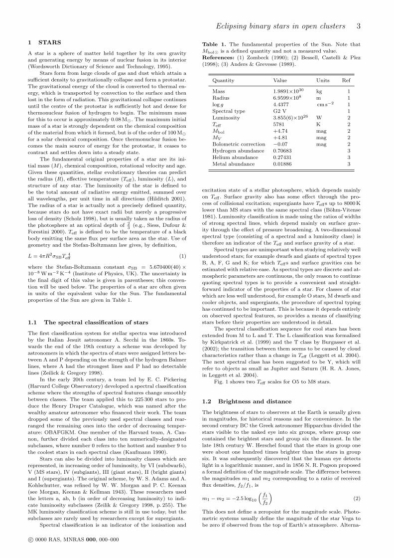
Fig. 1 shows two Teff scales for O5 to M8 stars.
1.2 Brightness and distance
The brightness of stars to observers at the Earth is usually givenin magnitudes, for historical reasons and for convenience. In thesecond century BC the Greek astronomer Hipparchus divided thestars visible to the naked eye into six groups, where group onecontained the brightest stars and group six the dimmest. In thelate 18th century W. Herschel found that the stars in group onewere about one hundred times brighter than the stars in groupsix. It was subsequently discovered that the human eye detectslight in a logarithmic manner, and in 1856 N. R. Pogson proposeda formal definition of the magnitude scale. The difference betweenthe magnitudes m1 and m2 corresponding to a ratio of receivedflux densities, f2/f1, is
m1 −m2 = −2.5 log10
(f1
f2
)(2)
This does not define a zeropoint for the magnitude scale. Photo-metric systems usually define the magnitude of the star Vega tobe zero if observed from the top of Earth’s atmosphere. Alterna-
c© 0000 RAS, MNRAS 000, 000–000
4 J. K. Taylor
Figure 1. Two Teff scales plotted against spectral type. The Teff
scales from Allen (1973) are plotted for (in decreasing Teff) MS,giant and supergiant stars (dotted lines). The Teff scales fromZombeck (1990) are plotted for (in decreasing Teff) MS and giantstars (dashed lines).
tive systems exist based on a more useful physical definition, e.g.,the ABν system used by the Sloan Digital Sky Survey (Oke &Gunn 1983; Fukugita et al. 1996).
As stars generally have a different spectral energy distribu-tion to Vega, the magnitudes of stars relative to Vega depend onthe wavelength at which observations are undertaken. The usualconvention is to use the visual magnitudes of stars, which is takento be the magnitude as viewed through the Johnson V passband(see Sec. 12), and denoted as mV . The absolute magnitude of astar is a measure of its intrinsic brightness and is defined to bethe apparent magnitude of the stars as viewed from a distance often parsecs. Using eq. 2 gives the equation
mV −MV = 5 log10(d)− 5 (3)
where d is the distance in parsecs and the quantity (mV −MV )is the apparent distance modulus.
The absolute magnitude of a star when considering the ra-ditation it emits summed over all wavelengths is the absolutebolometric magnitude (Mbol). This is usually given relative tothe Sun using the equation
Mbol −Mbol¯ = −2.5 log10
(L
L¯
)(4)
The relation between the absolute visual magnitude, MV , andabsolute bolometric magnitude, Mbol, of a star is
MV = Mbol −BCV (5)
where BCV is the V -band bolometric correction (see Sec. 1.3.5)
Colour indices for stars are the ratio of flux densities at twodifferent wavelengths (or viewed through two different passbands)relative to Vega, for example the colour index for a star betweenthe B and V passbands is
mB −mV = −2.5 log10
[(fB
fV
)star
(fV
fB
)Vega
](6)
The colour indices for Vega are all zero by definition.
1.2.1 Interstellar extinction
The matter between stars attenuates the light which passesthrough it. The amount of light which is attenuated is a func-tion of wavelength, so interstellar material affects the colours ofstars as well as their apparent brightnesses. The main attenua-tion is due to scattering, but some light is also absorbed. As blue
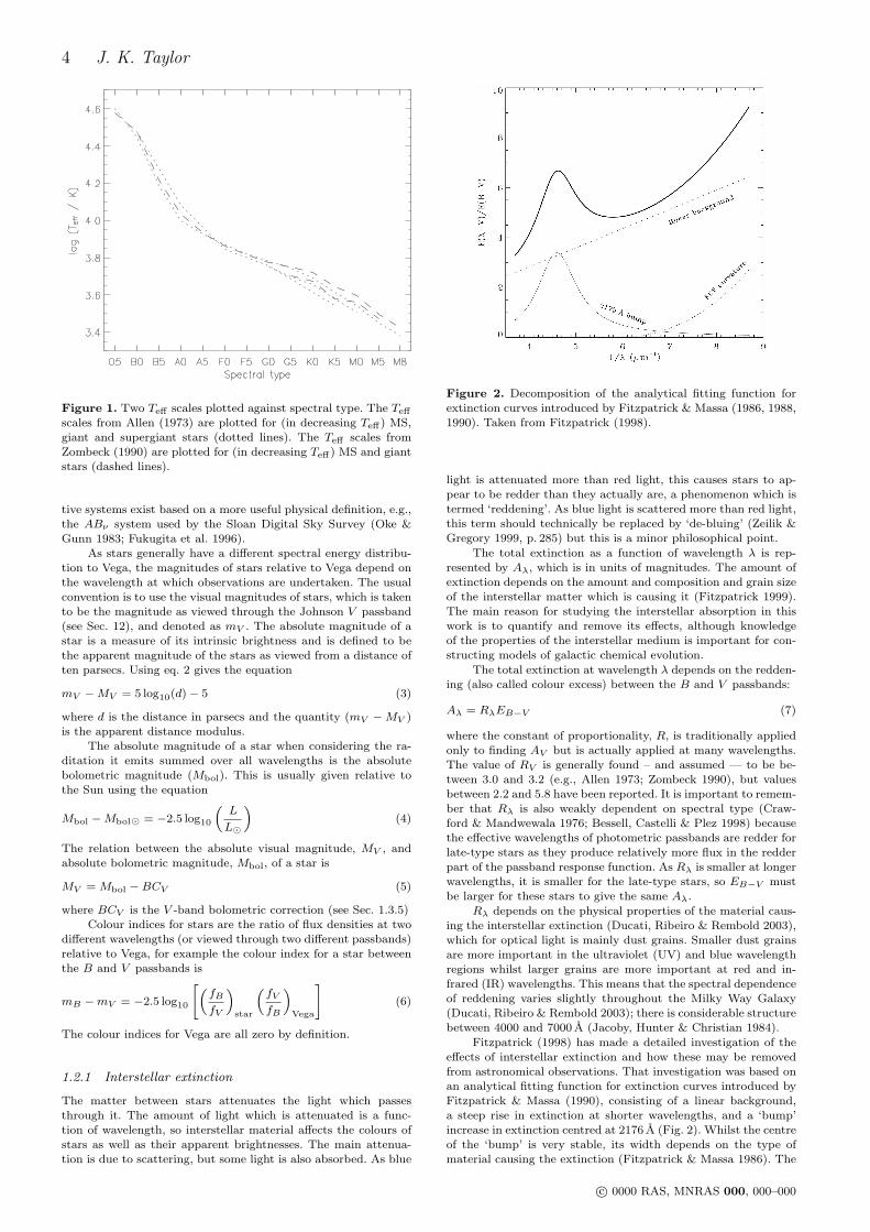
Figure 2. Decomposition of the analytical fitting function forextinction curves introduced by Fitzpatrick & Massa (1986, 1988,1990). Taken from Fitzpatrick (1998).
light is attenuated more than red light, this causes stars to ap-pear to be redder than they actually are, a phenomenon which istermed ‘reddening’. As blue light is scattered more than red light,this term should technically be replaced by ‘de-bluing’ (Zeilik &Gregory 1999, p. 285) but this is a minor philosophical point.
The total extinction as a function of wavelength λ is rep-resented by Aλ, which is in units of magnitudes. The amount ofextinction depends on the amount and composition and grain sizeof the interstellar matter which is causing it (Fitzpatrick 1999).The main reason for studying the interstellar absorption in thiswork is to quantify and remove its effects, although knowledgeof the properties of the interstellar medium is important for con-structing models of galactic chemical evolution.
The total extinction at wavelength λ depends on the redden-ing (also called colour excess) between the B and V passbands:
Aλ = RλEB−V (7)
where the constant of proportionality, R, is traditionally appliedonly to finding AV but is actually applied at many wavelengths.The value of RV is generally found – and assumed — to be be-tween 3.0 and 3.2 (e.g., Allen 1973; Zombeck 1990), but valuesbetween 2.2 and 5.8 have been reported. It is important to remem-ber that Rλ is also weakly dependent on spectral type (Craw-ford & Mandwewala 1976; Bessell, Castelli & Plez 1998) becausethe effective wavelengths of photometric passbands are redder forlate-type stars as they produce relatively more flux in the redderpart of the passband response function. As Rλ is smaller at longerwavelengths, it is smaller for the late-type stars, so EB−V mustbe larger for these stars to give the same Aλ.
Rλ depends on the physical properties of the material caus-ing the interstellar extinction (Ducati, Ribeiro & Rembold 2003),which for optical light is mainly dust grains. Smaller dust grainsare more important in the ultraviolet (UV) and blue wavelengthregions whilst larger grains are more important at red and in-frared (IR) wavelengths. This means that the spectral dependenceof reddening varies slightly throughout the Milky Way Galaxy(Ducati, Ribeiro & Rembold 2003); there is considerable structurebetween 4000 and 7000 A (Jacoby, Hunter & Christian 1984).
Fitzpatrick (1998) has made a detailed investigation of theeffects of interstellar extinction and how these may be removedfrom astronomical observations. That investigation was based onan analytical fitting function for extinction curves introduced byFitzpatrick & Massa (1990), consisting of a linear background,a steep rise in extinction at shorter wavelengths, and a ‘bump’increase in extinction centred at 2176 A (Fig. 2). Whilst the centreof the ‘bump’ is very stable, its width depends on the type ofmaterial causing the extinction (Fitzpatrick & Massa 1986). The
c© 0000 RAS, MNRAS 000, 000–000
Eclipsing binary stars in open clusters 5
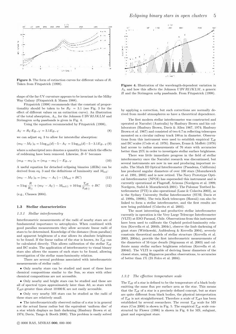
Figure 3. The form of extinction curves for different values of R.Taken from Fitzpatrick (1998).
shape of the far-UV curvature appears to be invariant in the MilkyWay Galaxy (Fitzpatrick & Massa 1988).
Fitzpatrick (1998) recommends that the constant of propor-tionality should be taken to be RV = 3.1 (see Fig. 3 for theeffect of different values on an extinction curve). An illustrationof the total absorption, Aλ, for the Johnson UBV RIJKLM andStromgren uvby passbands is given in Fig. 4.
Using the equation recommended by Fitzpatrick (1998),
AV = RV EB−V = 3.1EB−V (8)
we can adjust eq. 3 to allow for interstellar absorption:
(mV −MV )0 = 5 log10(d)−5−AV = 5 log10(d)−5−3.1EB−V (9)
where a subscripted zero denotes a quantity from which the effectsof reddening have been removed. Likewise, B−V becomes
(mB −mV )0 = (mB −mV )− EB−V (10)
A useful equation for detached eclipsing binaries (dEBs) can bederived from eq. 3 and the definitions of luminosity and Mbol:
(mV −MV )0 = (mV −AV )− (Mbol +BC) (11)
= 5 logR
R¯+ (mV −AV )−Mbol¯ + 10 log
Teff
Teff¯+BC (12)
(e.g., Clausen 2004).
1.3 Stellar characteristics
1.3.1 Stellar interferometry
Interferometric measurements of the radii of nearby stars are offundamental importance to astrophysics. When combined withgood parallax measurements they allow accurate linear radii ofstars to be determined. Knowledge of the distance (from parallax)and apparent brightness of a star allows its absolute brightnessto be found. If the linear radius of the star is known, its Teff canbe calculated directly. This allows calibration of the stellar Teff
and BC scales. The application of interferometry to visual binarystars also allows the masses of such stars to be found, allowinginvestigation of the stellar mass-luminosity relation.
There are several problems associated with interferometricmeasurements of stellar radii:–
• Only nearby stars can be studied and most of these havechemical compositions similar to the Sun, so stars with otherchemical compositions are not accessible.
• Only nearby and bright stars can be studied and these areall of spectral types approximately later than A0, so stars withTeffs greater than about 10 000 K are not easily accessible.
• Only very nearby MS stars can be studied as the radii ofthese stars are relatively small.
• The interferometrically observed radius of a star is in generalnot the actual linear radius but the equivalent ‘uniform disc’ ofa star which displays no limb darkening (Hanbury Brown et al.1974; Davis, Tango & Booth 2000). This problem is easily solved
Figure 4. Illustration of the wavelength-dependent variation inAλ and how this affects the Johnson UBV RIJKLM , a genericH and the Stromgren uvby passbands. From Fitzpatrick (1998).
by applying a correction, but such corrections are normally de-rived from model atmospheres so have a theoretical dependence.
The first modern stellar interferometer was constructed andoperated at Narrabri (Australia) by Hanbury Brown and his col-laborators (Hanbury Brown, Davis & Allen 1967, 1974; HanburyBrown et al. 1967) and consisted of two 6.7 m reflecting telescopesmounted on a circular railway track 188 m in diameter. Observa-tions from this instrument were used to establish empirical Teff
and BC scales (Code et al. 1976). Barnes, Evans & Moffett (1978)had access to radius measurements of 76 stars with accuraciesbetter than 25% in order to investigate stellar surface brightness.
There was little immediate progress in the field of stellarinterferometry once the Narrabri research was discontinued, butseveral instruments are now in use and producing important re-sults. The Mark III Optical Interferometer (Pasadena, California)has produced angular diameters of over 100 stars (Mozurkewichet al. 1991, 2003) and is now retired. The Navy Prototype Opti-cal Interferometer (NPOI) has superseded this instrument and iscurrently operational at Flagstaff, Arizona (Nordgren et al. 1999;Nordgren, Sudol & Mozurkewich 2001). The Palomar Testbed In-terferometer (PTI) is also operational (Lane & Colavita 2003), asis the Sydney University Stellar Interferometer (SUSI; Davis etal. 1999a, 1999b). The twin Keck telescopes (Hawaii) can also belinked to form a stellar interferometer, and the first results arenow being published (Colavita et al. 2003).
The most interesting and productive stellar interferometercurrently in operation is the Very Large Telescope Interferometer(VLTI) at ESO Paranal, Chile. Observations from this instrumenthave been used to calibrate the Cepheid period-luminosity rela-tion (Kervella et al. 2004b, 2004c), observe the limb darkening ofgiant stars (Wittkowski, Aufdenberg & Kervella 2004), severelyconstrain theoretical models of stellar structure (Kervella et al.2003, 2004a), provide the first interferometric measurements ofthe diameters of M-type dwarfs (Segransan et al. 2003) and cal-ibrate many stellar surface brightness relations (Kervella et al.2004d). The VLTI is capable of deriving linear diameters of theclosest stars, using Hipparcos parallax observations, to accuraciesof better than 1% (Di Folco et al. 2004).
1.3.2 The effective temperature scale
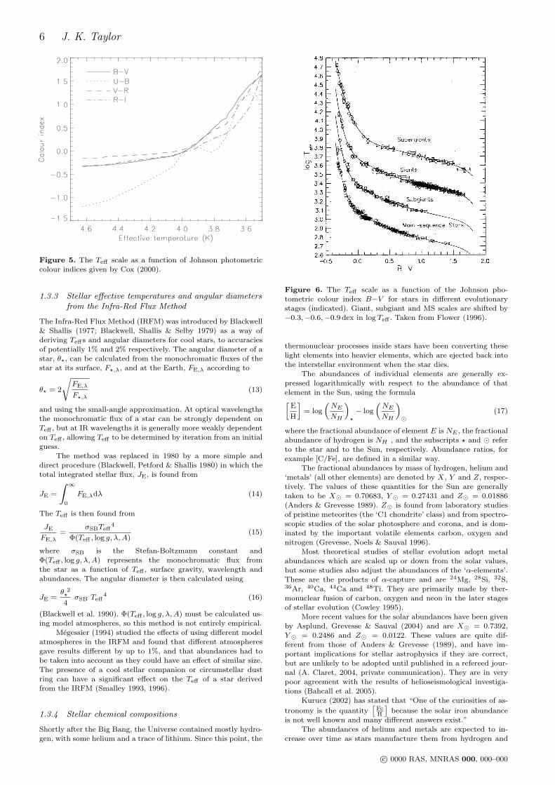
The Teff of a star is defined to be the temperature of a black bodyemitting the same flux per surface area as the star. This meansthat the Teff of a star is a precisely defined concept, but as starsare quite different from black bodies, the physical interpretationof Teff is not straightforward. Therefore a scale of Teffs has beenestablished by several researchers. The recent Teff scale for MSstars (Cox 2000) is shown in Fig. 5. The empirical Teff scale con-structed by Flower (1996) is shown in Fig. 6 for MS, subgiant,giant and supergiant stars.
c© 0000 RAS, MNRAS 000, 000–000
6 J. K. Taylor
Figure 5. The Teff scale as a function of Johnson photometriccolour indices given by Cox (2000).
1.3.3 Stellar effective temperatures and angular diametersfrom the Infra-Red Flux Method
The Infra-Red Flux Method (IRFM) was introduced by Blackwell& Shallis (1977; Blackwell, Shallis & Selby 1979) as a way ofderiving Teffs and angular diameters for cool stars, to accuraciesof potentially 1% and 2% respectively. The angular diameter of astar, θ?, can be calculated from the monochromatic fluxes of thestar at its surface, F?,λ, and at the Earth, FE,λ according to
θ? = 2
√FE,λ
F?,λ(13)
and using the small-angle approximation. At optical wavelengthsthe monochromatic flux of a star can be strongly dependent onTeff , but at IR wavelengths it is generally more weakly dependenton Teff , allowing Teff to be determined by iteration from an initialguess.
The method was replaced in 1980 by a more simple anddirect procedure (Blackwell, Petford & Shallis 1980) in which thetotal integrated stellar flux, JE, is found from
JE =
∫ ∞
0
FE,λdλ (14)
The Teff is then found from
JE
FE,λ=
σSBTeff4
Φ(Teff , log g, λ,A)(15)
where σSB is the Stefan-Boltzmann constant andΦ(Teff , log g, λ,A) represents the monochromatic flux fromthe star as a function of Teff , surface gravity, wavelength andabundances. The angular diameter is then calculated using
JE =θ 2?
4σSB Teff
4 (16)
(Blackwell et al. 1990). Φ(Teff , log g, λ,A) must be calculated us-ing model atmospheres, so this method is not entirely empirical.
Megessier (1994) studied the effects of using different modelatmospheres in the IRFM and found that different atmospheresgave results different by up to 1%, and that abundances had tobe taken into account as they could have an effect of similar size.The presence of a cool stellar companion or circumstellar dustring can have a significant effect on the Teff of a star derivedfrom the IRFM (Smalley 1993, 1996).
1.3.4 Stellar chemical compositions
Shortly after the Big Bang, the Universe contained mostly hydro-gen, with some helium and a trace of lithium. Since this point, the
Figure 6. The Teff scale as a function of the Johnson pho-tometric colour index B−V for stars in different evolutionarystages (indicated). Giant, subgiant and MS scales are shifted by−0.3,−0.6,−0.9 dex in log Teff . Taken from Flower (1996).
thermonuclear processes inside stars have been converting theselight elements into heavier elements, which are ejected back intothe interstellar environment when the star dies.
The abundances of individual elements are generally ex-pressed logarithmically with respect to the abundance of thatelement in the Sun, using the formula[
E
H
]= log
(NE
NH
)?
− log
(NE
NH
)¯
(17)
where the fractional abundance of element E is NE , the fractionalabundance of hydrogen is NH , and the subscripts ? and ¯ referto the star and to the Sun, respectively. Abundance ratios, forexample [C/Fe], are defined in a similar way.
The fractional abundances by mass of hydrogen, helium and‘metals’ (all other elements) are denoted by X, Y and Z, respec-tively. The values of these quantities for the Sun are generallytaken to be X¯ = 0.70683, Y ¯ = 0.27431 and Z¯ = 0.01886(Anders & Grevesse 1989). Z¯ is found from laboratory studiesof pristine meteorites (the ‘C1 chondrite’ class) and from spectro-scopic studies of the solar photosphere and corona, and is dom-inated by the important volatile elements carbon, oxygen andnitrogen (Grevesse, Noels & Sauval 1996).
Most theoretical studies of stellar evolution adopt metalabundances which are scaled up or down from the solar values,but some studies also adjust the abundances of the ‘α-elements’.These are the products of α-capture and are 24Mg, 28Si, 32S,36Ar, 40Ca, 44Ca and 48Ti. They are primarily made by ther-monuclear fusion of carbon, oxygen and neon in the later stagesof stellar evolution (Cowley 1995).
More recent values for the solar abundances have been givenby Asplund, Grevesse & Sauval (2004) and are X¯ = 0.7392,Y ¯ = 0.2486 and Z¯ = 0.0122. These values are quite dif-ferent from those of Anders & Grevesse (1989), and have im-portant implications for stellar astrophysics if they are correct,but are unlikely to be adopted until published in a refereed jour-nal (A. Claret, 2004, private communication). They are in verypoor agreement with the results of helioseismological investiga-tions (Bahcall et al. 2005).
Kurucz (2002) has stated that “One of the curiosities of as-
tronomy is the quantity[
FeH
]because the solar iron abundance
is not well known and many different answers exist.”
The abundances of helium and metals are expected to in-crease over time as stars manufacture them from hydrogen and
c© 0000 RAS, MNRAS 000, 000–000
Eclipsing binary stars in open clusters 7
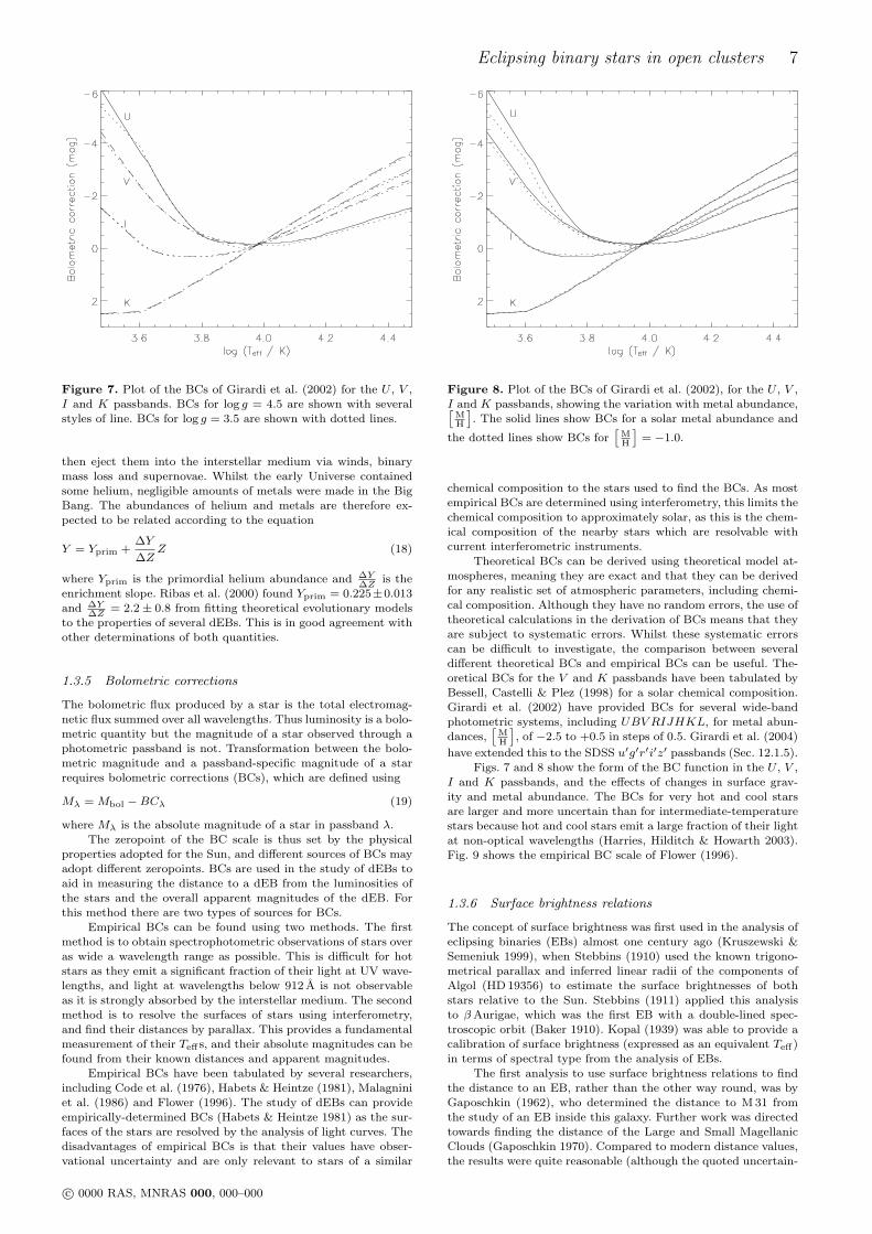
Figure 7. Plot of the BCs of Girardi et al. (2002) for the U , V ,I and K passbands. BCs for log g = 4.5 are shown with severalstyles of line. BCs for log g = 3.5 are shown with dotted lines.
then eject them into the interstellar medium via winds, binarymass loss and supernovae. Whilst the early Universe containedsome helium, negligible amounts of metals were made in the BigBang. The abundances of helium and metals are therefore ex-pected to be related according to the equation
Y = Yprim +∆Y
∆ZZ (18)
where Yprim is the primordial helium abundance and ∆Y∆Z
is theenrichment slope. Ribas et al. (2000) found Yprim = 0.225±0.013and ∆Y
∆Z= 2.2± 0.8 from fitting theoretical evolutionary models
to the properties of several dEBs. This is in good agreement withother determinations of both quantities.
1.3.5 Bolometric corrections
The bolometric flux produced by a star is the total electromag-netic flux summed over all wavelengths. Thus luminosity is a bolo-metric quantity but the magnitude of a star observed through aphotometric passband is not. Transformation between the bolo-metric magnitude and a passband-specific magnitude of a starrequires bolometric corrections (BCs), which are defined using
Mλ = Mbol −BCλ (19)
where Mλ is the absolute magnitude of a star in passband λ.
The zeropoint of the BC scale is thus set by the physicalproperties adopted for the Sun, and different sources of BCs mayadopt different zeropoints. BCs are used in the study of dEBs toaid in measuring the distance to a dEB from the luminosities ofthe stars and the overall apparent magnitudes of the dEB. Forthis method there are two types of sources for BCs.
Empirical BCs can be found using two methods. The firstmethod is to obtain spectrophotometric observations of stars overas wide a wavelength range as possible. This is difficult for hotstars as they emit a significant fraction of their light at UV wave-lengths, and light at wavelengths below 912 A is not observableas it is strongly absorbed by the interstellar medium. The secondmethod is to resolve the surfaces of stars using interferometry,and find their distances by parallax. This provides a fundamentalmeasurement of their Teffs, and their absolute magnitudes can befound from their known distances and apparent magnitudes.
Empirical BCs have been tabulated by several researchers,including Code et al. (1976), Habets & Heintze (1981), Malagniniet al. (1986) and Flower (1996). The study of dEBs can provideempirically-determined BCs (Habets & Heintze 1981) as the sur-faces of the stars are resolved by the analysis of light curves. Thedisadvantages of empirical BCs is that their values have obser-vational uncertainty and are only relevant to stars of a similar
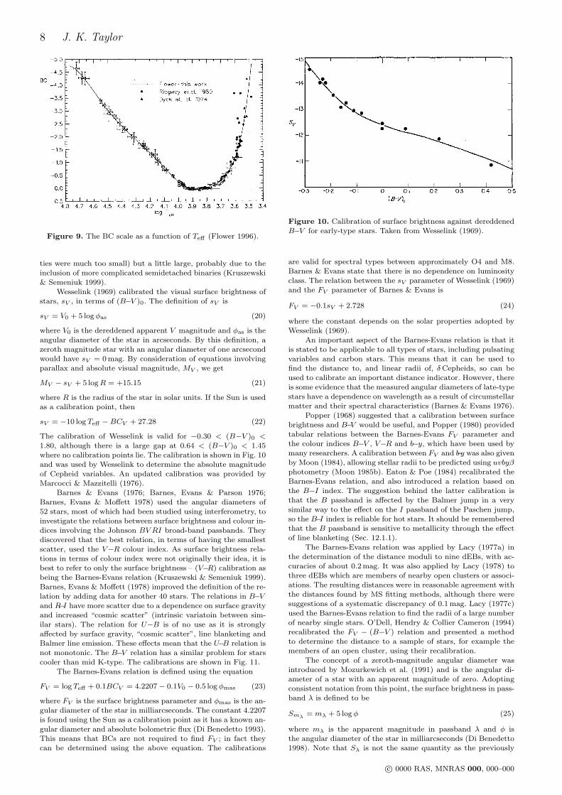
Figure 8. Plot of the BCs of Girardi et al. (2002), for the U , V ,I and K passbands, showing the variation with metal abundance,[
MH
]. The solid lines show BCs for a solar metal abundance and
the dotted lines show BCs for[
MH
]= −1.0.
chemical composition to the stars used to find the BCs. As mostempirical BCs are determined using interferometry, this limits thechemical composition to approximately solar, as this is the chem-ical composition of the nearby stars which are resolvable withcurrent interferometric instruments.
Theoretical BCs can be derived using theoretical model at-mospheres, meaning they are exact and that they can be derivedfor any realistic set of atmospheric parameters, including chemi-cal composition. Although they have no random errors, the use oftheoretical calculations in the derivation of BCs means that theyare subject to systematic errors. Whilst these systematic errorscan be difficult to investigate, the comparison between severaldifferent theoretical BCs and empirical BCs can be useful. The-oretical BCs for the V and K passbands have been tabulated byBessell, Castelli & Plez (1998) for a solar chemical composition.Girardi et al. (2002) have provided BCs for several wide-bandphotometric systems, including UBV RIJHKL, for metal abun-dances,
[MH
], of −2.5 to +0.5 in steps of 0.5. Girardi et al. (2004)
have extended this to the SDSS u′g′r′i′z′ passbands (Sec. 12.1.5).
Figs. 7 and 8 show the form of the BC function in the U , V ,I and K passbands, and the effects of changes in surface grav-ity and metal abundance. The BCs for very hot and cool starsare larger and more uncertain than for intermediate-temperaturestars because hot and cool stars emit a large fraction of their lightat non-optical wavelengths (Harries, Hilditch & Howarth 2003).Fig. 9 shows the empirical BC scale of Flower (1996).
1.3.6 Surface brightness relations
The concept of surface brightness was first used in the analysis ofeclipsing binaries (EBs) almost one century ago (Kruszewski &Semeniuk 1999), when Stebbins (1910) used the known trigono-metrical parallax and inferred linear radii of the components ofAlgol (HD 19356) to estimate the surface brightnesses of bothstars relative to the Sun. Stebbins (1911) applied this analysisto βAurigae, which was the first EB with a double-lined spec-troscopic orbit (Baker 1910). Kopal (1939) was able to provide acalibration of surface brightness (expressed as an equivalent Teff)in terms of spectral type from the analysis of EBs.
The first analysis to use surface brightness relations to findthe distance to an EB, rather than the other way round, was byGaposchkin (1962), who determined the distance to M 31 fromthe study of an EB inside this galaxy. Further work was directedtowards finding the distance of the Large and Small MagellanicClouds (Gaposchkin 1970). Compared to modern distance values,the results were quite reasonable (although the quoted uncertain-
c© 0000 RAS, MNRAS 000, 000–000
8 J. K. Taylor
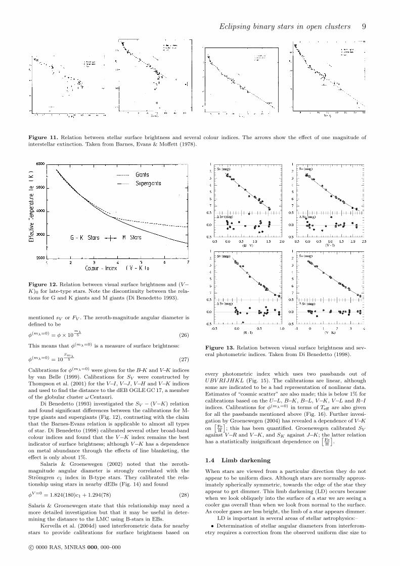
Figure 9. The BC scale as a function of Teff (Flower 1996).
ties were much too small) but a little large, probably due to theinclusion of more complicated semidetached binaries (Kruszewski& Semeniuk 1999).
Wesselink (1969) calibrated the visual surface brightness ofstars, sV , in terms of (B−V )0. The definition of sV is
sV = V0 + 5 log φas (20)
where V0 is the dereddened apparent V magnitude and φas is theangular diameter of the star in arcseconds. By this definition, azeroth magnitude star with an angular diameter of one arcsecondwould have sV = 0 mag. By consideration of equations involvingparallax and absolute visual magnitude, MV , we get
MV − sV + 5 logR = +15.15 (21)
where R is the radius of the star in solar units. If the Sun is usedas a calibration point, then
sV = −10 log Teff −BCV + 27.28 (22)
The calibration of Wesselink is valid for −0.30 < (B−V )0 <1.80, although there is a large gap at 0.64 < (B−V )0 < 1.45where no calibration points lie. The calibration is shown in Fig. 10and was used by Wesselink to determine the absolute magnitudeof Cepheid variables. An updated calibration was provided byMarcocci & Mazzitelli (1976).
Barnes & Evans (1976; Barnes, Evans & Parson 1976;Barnes, Evans & Moffett 1978) used the angular diameters of52 stars, most of which had been studied using interferometry, toinvestigate the relations between surface brightness and colour in-dices involving the Johnson BV RI broad-band passbands. Theydiscovered that the best relation, in terms of having the smallestscatter, used the V−R colour index. As surface brightness rela-tions in terms of colour index were not originally their idea, it isbest to refer to only the surface brightness – (V−R) calibration asbeing the Barnes-Evans relation (Kruszewski & Semeniuk 1999).Barnes, Evans & Moffett (1978) improved the definition of the re-lation by adding data for another 40 stars. The relations in B−Vand R−I have more scatter due to a dependence on surface gravityand increased “cosmic scatter” (intrinsic variatoin between sim-ilar stars). The relation for U−B is of no use as it is stronglyaffected by surface gravity, “cosmic scatter”, line blanketing andBalmer line emission. These effects mean that the U−B relation isnot monotonic. The B−V relation has a similar problem for starscooler than mid K-type. The calibrations are shown in Fig. 11.
The Barnes-Evans relation is defined using the equation
FV = log Teff + 0.1BCV = 4.2207− 0.1V0 − 0.5 log φmas (23)
where FV is the surface brightness parameter and φmas is the an-gular diameter of the star in milliarcseconds. The constant 4.2207is found using the Sun as a calibration point as it has a known an-gular diameter and absolute bolometric flux (Di Benedetto 1993).This means that BCs are not required to find FV ; in fact theycan be determined using the above equation. The calibrations
Figure 10. Calibration of surface brightness against dereddenedB−V for early-type stars. Taken from Wesselink (1969).
are valid for spectral types between approximately O4 and M8.Barnes & Evans state that there is no dependence on luminosityclass. The relation between the sV parameter of Wesselink (1969)and the FV parameter of Barnes & Evans is
FV = −0.1sV + 2.728 (24)
where the constant depends on the solar properties adopted byWesselink (1969).
An important aspect of the Barnes-Evans relation is that itis stated to be applicable to all types of stars, including pulsatingvariables and carbon stars. This means that it can be used tofind the distance to, and linear radii of, δCepheids, so can beused to calibrate an important distance indicator. However, thereis some evidence that the measured angular diameters of late-typestars have a dependence on wavelength as a result of circumstellarmatter and their spectral characteristics (Barnes & Evans 1976).
Popper (1968) suggested that a calibration between surfacebrightness and B−V would be useful, and Popper (1980) providedtabular relations between the Barnes-Evans FV parameter andthe colour indices B−V , V−R and b−y, which have been used bymany researchers. A calibration between FV and b−y was also givenby Moon (1984), allowing stellar radii to be predicted using uvbyβphotometry (Moon 1985b). Eaton & Poe (1984) recalibrated theBarnes-Evans relation, and also introduced a relation based onthe B−I index. The suggestion behind the latter calibration isthat the B passband is affected by the Balmer jump in a verysimilar way to the effect on the I passband of the Paschen jump,so the B−I index is reliable for hot stars. It should be rememberedthat the B passband is sensitive to metallicity through the effectof line blanketing (Sec. 12.1.1).
The Barnes-Evans relation was applied by Lacy (1977a) inthe determination of the distance moduli to nine dEBs, with ac-curacies of about 0.2 mag. It was also applied by Lacy (1978) tothree dEBs which are members of nearby open clusters or associ-ations. The resulting distances were in reasonable agreement withthe distances found by MS fitting methods, although there weresuggestions of a systematic discrepancy of 0.1 mag. Lacy (1977c)used the Barnes-Evans relation to find the radii of a large numberof nearby single stars. O’Dell, Hendry & Collier Cameron (1994)recalibrated the FV − (B−V ) relation and presented a methodto determine the distance to a sample of stars, for example themembers of an open cluster, using their recalibration.
The concept of a zeroth-magnitude angular diameter wasintroduced by Mozurkewich et al. (1991) and is the angular di-ameter of a star with an apparent magnitude of zero. Adoptingconsistent notation from this point, the surface brightness in pass-band λ is defined to be
Smλ = mλ + 5 log φ (25)
where mλ is the apparent magnitude in passband λ and φ isthe angular diameter of the star in milliarcseconds (Di Benedetto1998). Note that Sλ is not the same quantity as the previously
c© 0000 RAS, MNRAS 000, 000–000
Eclipsing binary stars in open clusters 9
Figure 11. Relation between stellar surface brightness and several colour indices. The arrows show the effect of one magnitude ofinterstellar extinction. Taken from Barnes, Evans & Moffett (1978).
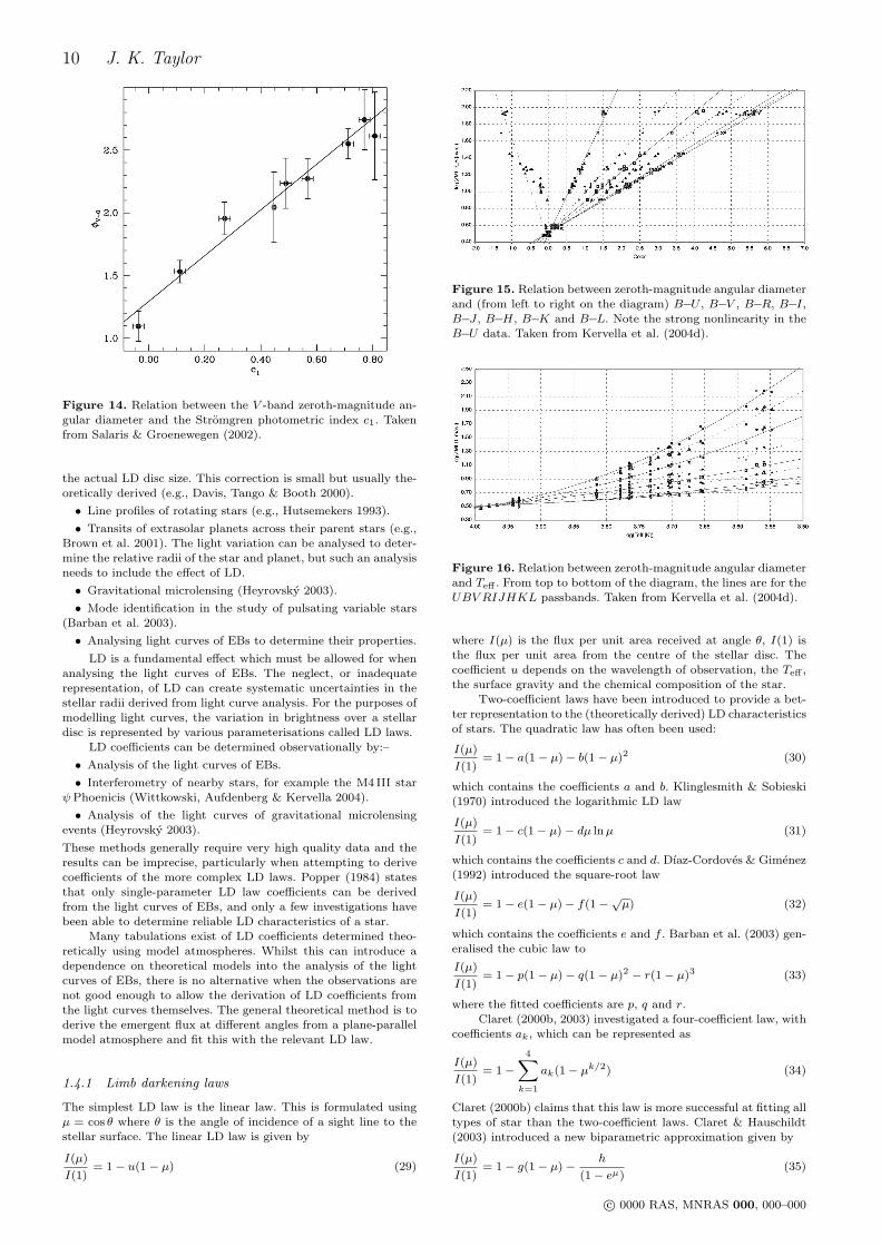
Figure 12. Relation between visual surface brightness and (V−K)0 for late-type stars. Note the discontinuity between the rela-tions for G and K giants and M giants (Di Benedetto 1993).
mentioned sV or FV . The zeroth-magnitude angular diameter isdefined to be
φ(mλ=0) = φ× 10mλ5 (26)
This means that φ(mλ=0) is a measure of surface brightness:
φ(mλ=0) = 10Smλ
5 (27)
Calibrations for φ(mλ=0) were given for the B−K and V−K indicesby van Belle (1999). Calibrations for SV were constructed byThompson et al. (2001) for the V−I, V−J , V−H and V−K indicesand used to find the distance to the dEB OGLE GC 17, a memberof the globular cluster ωCentauri.
Di Benedetto (1993) investigated the SV − (V−K) relationand found significant differences between the calibrations for M-type giants and supergiants (Fig. 12), contrasting with the claimthat the Barnes-Evans relation is applicable to almost all typesof star. Di Benedetto (1998) calibrated several other broad-bandcolour indices and found that the V−K index remains the bestindicator of surface brightness; although V−K has a dependenceon metal abundance through the effects of line blanketing, theeffect is only about 1%.
Salaris & Groenewegen (2002) noted that the zeroth-magnitude angular diameter is strongly correlated with theStromgren c1 index in B-type stars. They calibrated the rela-tionship using stars in nearby dEBs (Fig. 14) and found
φV =0 = 1.824(180)c1 + 1.294(78) (28)
Salaris & Groenewegen state that this relationship may need amore detailed investigation but that it may be useful in deter-mining the distance to the LMC using B-stars in EBs.
Kervella et al. (2004d) used interferometric data for nearbystars to provide calibrations for surface brightness based on
Figure 13. Relation between visual surface brightness and sev-eral photometric indices. Taken from Di Benedetto (1998).
every photometric index which uses two passbands out ofUBV RIJHKL (Fig. 15). The calibrations are linear, althoughsome are indicated to be a bad representation of nonlinear data.Estimates of “cosmic scatter” are also made; this is below 1% forcalibrations based on the U−L, B−K, B−L, V−K, V−L and R−Iindices. Calibrations for φ(mλ=0) in terms of Teff are also givenfor all the passbands mentioned above (Fig. 16). Further invesi-gation by Groenewegen (2004) has revealed a dependence of V−Kon
[FeH
]; this has been quantified. Groenewegen calibrated SV
against V−R and V−K, and SK against J−K; the latter relationhas a statistically insignificant dependence on
[FeH
].
1.4 Limb darkening
When stars are viewed from a particular direction they do notappear to be uniform discs. Although stars are normally approx-imately spherically symmetric, towards the edge of the star theyappear to get dimmer. This limb darkening (LD) occurs becausewhen we look obliquely into the surface of a star we are seeing acooler gas overall than when we look from normal to the surface.As cooler gases are less bright, the limb of a star appears dimmer.
LD is important in several areas of stellar astrophysics:–
• Determination of stellar angular diameters from interferom-etry requires a correction from the observed uniform disc size to
c© 0000 RAS, MNRAS 000, 000–000
10 J. K. Taylor
Figure 14. Relation between the V -band zeroth-magnitude an-gular diameter and the Stromgren photometric index c1. Takenfrom Salaris & Groenewegen (2002).
the actual LD disc size. This correction is small but usually the-oretically derived (e.g., Davis, Tango & Booth 2000).
• Line profiles of rotating stars (e.g., Hutsemekers 1993).
• Transits of extrasolar planets across their parent stars (e.g.,Brown et al. 2001). The light variation can be analysed to deter-mine the relative radii of the star and planet, but such an analysisneeds to include the effect of LD.
• Gravitational microlensing (Heyrovsky 2003).
• Mode identification in the study of pulsating variable stars(Barban et al. 2003).
• Analysing light curves of EBs to determine their properties.
LD is a fundamental effect which must be allowed for whenanalysing the light curves of EBs. The neglect, or inadequaterepresentation, of LD can create systematic uncertainties in thestellar radii derived from light curve analysis. For the purposes ofmodelling light curves, the variation in brightness over a stellardisc is represented by various parameterisations called LD laws.
LD coefficients can be determined observationally by:–
• Analysis of the light curves of EBs.
• Interferometry of nearby stars, for example the M4 III starψPhoenicis (Wittkowski, Aufdenberg & Kervella 2004).
• Analysis of the light curves of gravitational microlensingevents (Heyrovsky 2003).
These methods generally require very high quality data and theresults can be imprecise, particularly when attempting to derivecoefficients of the more complex LD laws. Popper (1984) statesthat only single-parameter LD law coefficients can be derivedfrom the light curves of EBs, and only a few investigations havebeen able to determine reliable LD characteristics of a star.
Many tabulations exist of LD coefficients determined theo-retically using model atmospheres. Whilst this can introduce adependence on theoretical models into the analysis of the lightcurves of EBs, there is no alternative when the observations arenot good enough to allow the derivation of LD coefficients fromthe light curves themselves. The general theoretical method is toderive the emergent flux at different angles from a plane-parallelmodel atmosphere and fit this with the relevant LD law.
1.4.1 Limb darkening laws
The simplest LD law is the linear law. This is formulated usingµ = cos θ where θ is the angle of incidence of a sight line to thestellar surface. The linear LD law is given by
I(µ)
I(1)= 1− u(1− µ) (29)
Figure 15. Relation between zeroth-magnitude angular diameterand (from left to right on the diagram) B−U , B−V , B−R, B−I,B−J , B−H, B−K and B−L. Note the strong nonlinearity in theB−U data. Taken from Kervella et al. (2004d).
Figure 16. Relation between zeroth-magnitude angular diameterand Teff . From top to bottom of the diagram, the lines are for theUBV RIJHKL passbands. Taken from Kervella et al. (2004d).
where I(µ) is the flux per unit area received at angle θ, I(1) isthe flux per unit area from the centre of the stellar disc. Thecoefficient u depends on the wavelength of observation, the Teff ,the surface gravity and the chemical composition of the star.
Two-coefficient laws have been introduced to provide a bet-ter representation to the (theoretically derived) LD characteristicsof stars. The quadratic law has often been used:
I(µ)
I(1)= 1− a(1− µ)− b(1− µ)2 (30)
which contains the coefficients a and b. Klinglesmith & Sobieski(1970) introduced the logarithmic LD law
I(µ)
I(1)= 1− c(1− µ)− dµ lnµ (31)
which contains the coefficients c and d. Dıaz-Cordoves & Gimenez(1992) introduced the square-root law
I(µ)
I(1)= 1− e(1− µ)− f(1−√µ) (32)
which contains the coefficients e and f . Barban et al. (2003) gen-eralised the cubic law to
I(µ)
I(1)= 1− p(1− µ)− q(1− µ)2 − r(1− µ)3 (33)
where the fitted coefficients are p, q and r.Claret (2000b, 2003) investigated a four-coefficient law, with
coefficients ak, which can be represented as
I(µ)
I(1)= 1−
4∑k=1
ak(1− µk/2) (34)
Claret (2000b) claims that this law is more successful at fitting alltypes of star than the two-coefficient laws. Claret & Hauschildt(2003) introduced a new biparametric approximation given by
I(µ)
I(1)= 1− g(1− µ)− h
(1− eµ)(35)
c© 0000 RAS, MNRAS 000, 000–000
Eclipsing binary stars in open clusters 11
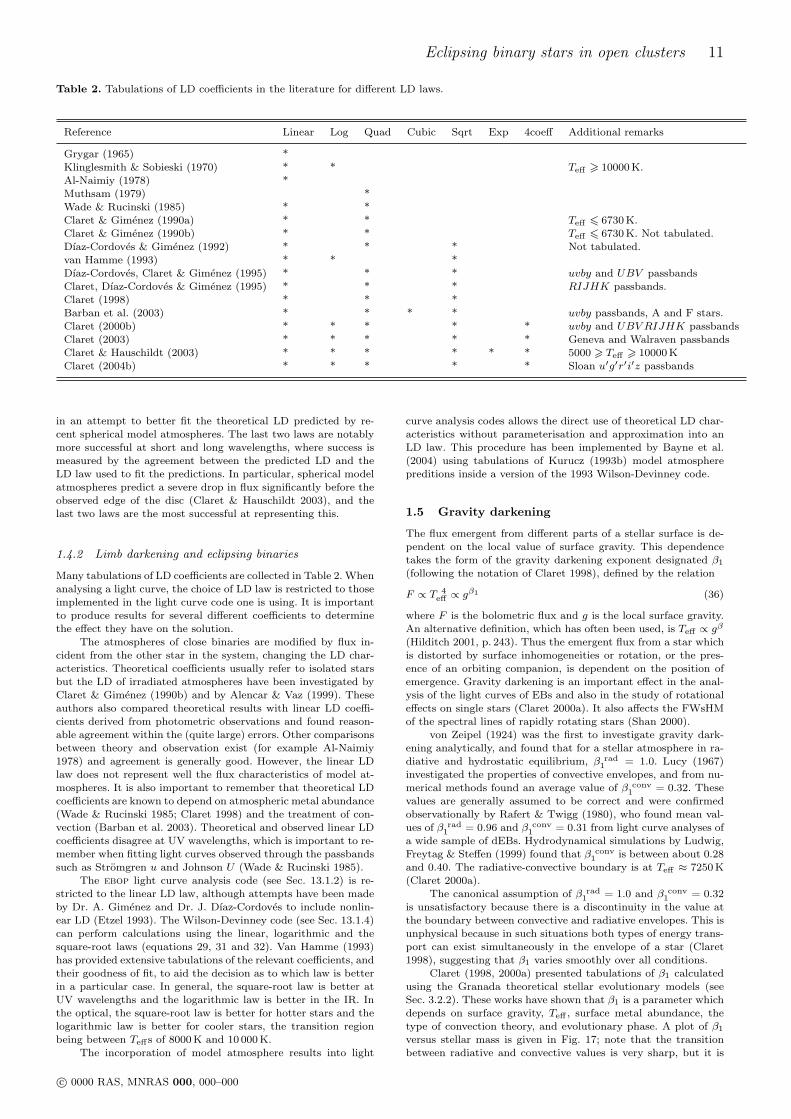
Table 2. Tabulations of LD coefficients in the literature for different LD laws.
Reference Linear Log Quad Cubic Sqrt Exp 4coeff Additional remarks
Grygar (1965) *Klinglesmith & Sobieski (1970) * * Teff > 10000 K.Al-Naimiy (1978) *Muthsam (1979) *Wade & Rucinski (1985) * *Claret & Gimenez (1990a) * * Teff 6 6730 K.Claret & Gimenez (1990b) * * Teff 6 6730 K. Not tabulated.Dıaz-Cordoves & Gimenez (1992) * * * Not tabulated.van Hamme (1993) * * *Dıaz-Cordoves, Claret & Gimenez (1995) * * * uvby and UBV passbandsClaret, Dıaz-Cordoves & Gimenez (1995) * * * RIJHK passbands.Claret (1998) * * *Barban et al. (2003) * * * * uvby passbands, A and F stars.Claret (2000b) * * * * * uvby and UBV RIJHK passbandsClaret (2003) * * * * * Geneva and Walraven passbandsClaret & Hauschildt (2003) * * * * * * 5000 > Teff > 10000 KClaret (2004b) * * * * * Sloan u′g′r′i′z passbands
in an attempt to better fit the theoretical LD predicted by re-cent spherical model atmospheres. The last two laws are notablymore successful at short and long wavelengths, where success ismeasured by the agreement between the predicted LD and theLD law used to fit the predictions. In particular, spherical modelatmospheres predict a severe drop in flux significantly before theobserved edge of the disc (Claret & Hauschildt 2003), and thelast two laws are the most successful at representing this.
1.4.2 Limb darkening and eclipsing binaries
Many tabulations of LD coefficients are collected in Table 2. Whenanalysing a light curve, the choice of LD law is restricted to thoseimplemented in the light curve code one is using. It is importantto produce results for several different coefficients to determinethe effect they have on the solution.
The atmospheres of close binaries are modified by flux in-cident from the other star in the system, changing the LD char-acteristics. Theoretical coefficients usually refer to isolated starsbut the LD of irradiated atmospheres have been investigated byClaret & Gimenez (1990b) and by Alencar & Vaz (1999). Theseauthors also compared theoretical results with linear LD coeffi-cients derived from photometric observations and found reason-able agreement within the (quite large) errors. Other comparisonsbetween theory and observation exist (for example Al-Naimiy1978) and agreement is generally good. However, the linear LDlaw does not represent well the flux characteristics of model at-mospheres. It is also important to remember that theoretical LDcoefficients are known to depend on atmospheric metal abundance(Wade & Rucinski 1985; Claret 1998) and the treatment of con-vection (Barban et al. 2003). Theoretical and observed linear LDcoefficients disagree at UV wavelengths, which is important to re-member when fitting light curves observed through the passbandssuch as Stromgren u and Johnson U (Wade & Rucinski 1985).
The ebop light curve analysis code (see Sec. 13.1.2) is re-stricted to the linear LD law, although attempts have been madeby Dr. A. Gimenez and Dr. J. Dıaz-Cordoves to include nonlin-ear LD (Etzel 1993). The Wilson-Devinney code (see Sec. 13.1.4)can perform calculations using the linear, logarithmic and thesquare-root laws (equations 29, 31 and 32). Van Hamme (1993)has provided extensive tabulations of the relevant coefficients, andtheir goodness of fit, to aid the decision as to which law is betterin a particular case. In general, the square-root law is better atUV wavelengths and the logarithmic law is better in the IR. Inthe optical, the square-root law is better for hotter stars and thelogarithmic law is better for cooler stars, the transition regionbeing between Teffs of 8000 K and 10 000 K.
The incorporation of model atmosphere results into light
curve analysis codes allows the direct use of theoretical LD char-acteristics without parameterisation and approximation into anLD law. This procedure has been implemented by Bayne et al.(2004) using tabulations of Kurucz (1993b) model atmospherepreditions inside a version of the 1993 Wilson-Devinney code.
1.5 Gravity darkening
The flux emergent from different parts of a stellar surface is de-pendent on the local value of surface gravity. This dependencetakes the form of the gravity darkening exponent designated β1
(following the notation of Claret 1998), defined by the relation
F ∝ T 4eff ∝ gβ1 (36)
where F is the bolometric flux and g is the local surface gravity.An alternative definition, which has often been used, is Teff ∝ gβ
(Hilditch 2001, p. 243). Thus the emergent flux from a star whichis distorted by surface inhomogeneities or rotation, or the pres-ence of an orbiting companion, is dependent on the position ofemergence. Gravity darkening is an important effect in the anal-ysis of the light curves of EBs and also in the study of rotationaleffects on single stars (Claret 2000a). It also affects the FWsHMof the spectral lines of rapidly rotating stars (Shan 2000).
von Zeipel (1924) was the first to investigate gravity dark-ening analytically, and found that for a stellar atmosphere in ra-diative and hydrostatic equilibrium, β rad
1 = 1.0. Lucy (1967)investigated the properties of convective envelopes, and from nu-merical methods found an average value of β conv
1 = 0.32. Thesevalues are generally assumed to be correct and were confirmedobservationally by Rafert & Twigg (1980), who found mean val-ues of β rad
1 = 0.96 and β conv1 = 0.31 from light curve analyses of
a wide sample of dEBs. Hydrodynamical simulations by Ludwig,Freytag & Steffen (1999) found that β conv
1 is between about 0.28and 0.40. The radiative-convective boundary is at Teff ≈ 7250 K(Claret 2000a).
The canonical assumption of β rad1 = 1.0 and β conv
1 = 0.32is unsatisfactory because there is a discontinuity in the value atthe boundary between convective and radiative envelopes. This isunphysical because in such situations both types of energy trans-port can exist simultaneously in the envelope of a star (Claret1998), suggesting that β1 varies smoothly over all conditions.
Claret (1998, 2000a) presented tabulations of β1 calculatedusing the Granada theoretical stellar evolutionary models (seeSec. 3.2.2). These works have shown that β1 is a parameter whichdepends on surface gravity, Teff , surface metal abundance, thetype of convection theory, and evolutionary phase. A plot of β1
versus stellar mass is given in Fig. 17; note that the transitionbetween radiative and convective values is very sharp, but it is
c© 0000 RAS, MNRAS 000, 000–000
12 J. K. Taylor
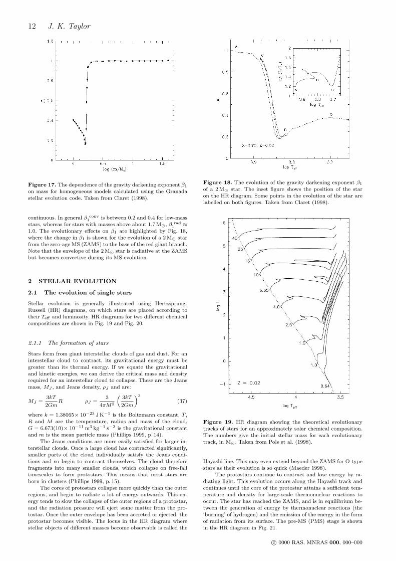
Figure 17. The dependence of the gravity darkening exponent β1
on mass for homogeneous models calculated using the Granadastellar evolution code. Taken from Claret (1998).
continuous. In general β conv1 is between 0.2 and 0.4 for low-mass
stars, whereas for stars with masses above about 1.7 M¯, β rad1 ≈
1.0. The evolutionary effects on β1 are highlighted by Fig. 18,where the change in β1 is shown for the evolution of a 2 M¯ starfrom the zero-age MS (ZAMS) to the base of the red giant branch.Note that the envelope of the 2 M¯ star is radiative at the ZAMSbut becomes convective during its MS evolution.
2 STELLAR EVOLUTION
2.1 The evolution of single stars
Stellar evolution is generally illustrated using Hertzsprung-Russell (HR) diagrams, on which stars are placed according totheir Teff and luminosity. HR diagrams for two different chemicalcompositions are shown in Fig. 19 and Fig. 20.
2.1.1 The formation of stars
Stars form from giant interstellar clouds of gas and dust. For aninterstellar cloud to contract, its gravitational energy must begreater than its thermal energy. If we equate the gravitationaland kinetic energies, we can derive the critical mass and densityrequired for an interstellar cloud to collapse. These are the Jeansmass, MJ , and Jeans density, ρJ and are:
MJ =3kT
2GmR ρJ =
3
4πM2
(3kT
2Gm
)3
(37)
where k = 1.38065× 10⁻²³ J K−1 is the Boltzmann constant, T ,R and M are the temperature, radius and mass of the cloud,G = 6.673(10)× 10−11 m3 kg−1 s−2 is the gravitational constantand m is the mean particle mass (Phillips 1999, p. 14).
The Jeans conditions are more easily satisfied for larger in-terstellar clouds. Once a large cloud has contracted significantly,smaller parts of the cloud individually satisfy the Jeans condi-tions and so begin to contract themselves. The cloud thereforefragments into many smaller clouds, which collapse on free-falltimescales to form protostars. This means that most stars areborn in clusters (Phillips 1999, p. 15).
The cores of protostars collapse more quickly than the outerregions, and begin to radiate a lot of energy outwards. This en-ergy tends to slow the collapse of the outer regions of a protostar,and the radiation pressure will eject some matter from the pro-tostar. Once the outer envelope has been accreted or ejected, theprotostar becomes visible. The locus in the HR diagram wherestellar objects of different masses become observable is called the
Figure 18. The evolution of the gravity darkening exponent β1
of a 2 M¯ star. The inset figure shows the position of the staron the HR diagram. Some points in the evolution of the star arelabelled on both figures. Taken from Claret (1998).
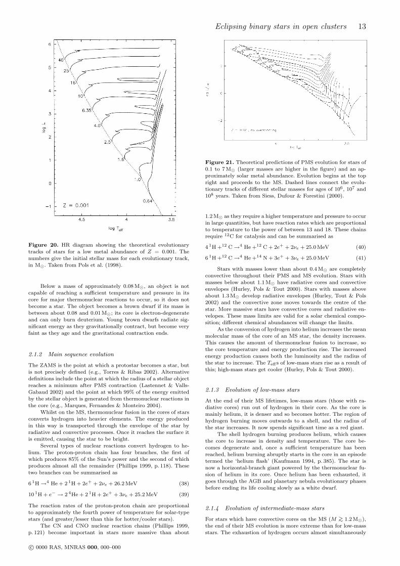
Figure 19. HR diagram showing the theoretical evolutionarytracks of stars for an approximately solar chemical composition.The numbers give the initial stellar mass for each evolutionarytrack, in M¯. Taken from Pols et al. (1998).
Hayashi line. This may even extend beyond the ZAMS for O-typestars as their evolution is so quick (Maeder 1998).
The protostars continue to contract and lose energy by ra-diating light. This evolution occurs along the Hayashi track andcontinues until the core of the protostar attains a sufficient tem-perature and density for large-scale thermonuclear reactions tooccur. The star has reached the ZAMS, and is in equilibrium be-tween the generation of energy by thermonuclear reactions (the‘burning’ of hydrogen) and the emission of the energy in the formof radiation from its surface. The pre-MS (PMS) stage is shownin the HR diagram in Fig. 21.
c© 0000 RAS, MNRAS 000, 000–000
Eclipsing binary stars in open clusters 13
Figure 20. HR diagram showing the theoretical evolutionarytracks of stars for a low metal abundance of Z = 0.001. Thenumbers give the initial stellar mass for each evolutionary track,in M¯. Taken from Pols et al. (1998).
Below a mass of approximately 0.08 M¯, an object is notcapable of reaching a sufficient temperature and pressure in itscore for major thermonuclear reactions to occur, so it does notbecome a star. The object becomes a brown dwarf if its mass isbetween about 0.08 and 0.01 M¯; its core is electron-degenerateand can only burn deuterium. Young brown dwarfs radiate sig-nificant energy as they gravitationally contract, but become veryfaint as they age and the gravitational contraction ends.
2.1.2 Main sequence evolution
The ZAMS is the point at which a protostar becomes a star, butis not precisely defined (e.g., Torres & Ribas 2002). Alternativedefinitions include the point at which the radius of a stellar objectreaches a minimum after PMS contraction (Lastennet & Valls-Gabaud 2002) and the point at which 99% of the energy emittedby the stellar object is generated from thermonuclear reactions inthe core (e.g., Marques, Fernandes & Monteiro 2004).
Whilst on the MS, thermonuclear fusion in the cores of starsconverts hydrogen into heavier elements. The energy producedin this way is transported through the envelope of the star byradiative and convective processes. Once it reaches the surface itis emitted, causing the star to be bright.
Several types of nuclear reactions convert hydrogen to he-lium. The proton-proton chain has four branches, the first ofwhich produces 85% of the Sun’s power and the second of whichproduces almost all the remainder (Phillips 1999, p. 118). Thesetwo branches can be summarised as
6 1H →4 He + 2 1H + 2e+ + 2νe + 26.2 MeV (38)
10 1H + e− → 2 4He + 2 1H + 2e+ + 3νe + 25.2 MeV (39)
The reaction rates of the proton-proton chain are proportionalto approximately the fourth power of temperature for solar-typestars (and greater/lesser than this for hotter/cooler stars).
The CN and CNO nuclear reaction chains (Phillips 1999,p. 121) become important in stars more massive than about
Figure 21. Theoretical predictions of PMS evolution for stars of0.1 to 7 M¯ (larger masses are higher in the figure) and an ap-proximately solar metal abundance. Evolution begins at the topright and proceeds to the MS. Dashed lines connect the evolu-tionary tracks of different stellar masses for ages of 106, 107 and108 years. Taken from Siess, Dufour & Forestini (2000).
1.2 M¯ as they require a higher temperature and pressure to occurin large quantities, but have reaction rates which are proportionalto temperature to the power of between 13 and 18. These chainsrequire 12C for catalysis and can be summarised as
4 1H +12 C →4 He +12 C + 2e+ + 2νe + 25.0 MeV (40)
6 1H +12 C →4 He +14 N + 3e+ + 3νe + 25.0 MeV (41)
Stars with masses lower than about 0.4 M¯ are completelyconvective throughout their PMS and MS evolution. Stars withmasses below about 1.1 M¯ have radiative cores and convectiveenvelopes (Hurley, Pols & Tout 2000). Stars with masses aboveabout 1.3 M¯ develop radiative envelopes (Hurley, Tout & Pols2002) and the convective zone moves towards the centre of thestar. More massive stars have convective cores and radiative en-velopes. These mass limits are valid for a solar chemical compo-sition; different chemical abundances will change the limits.
As the conversion of hydrogen into helium increases the meanmolecular mass of the core of an MS star, the density increases.This causes the amount of thermonuclear fusion to increase, sothe core temperature and energy production rise. The increasedenergy production causes both the luminosity and the radius ofthe star to increase. The Teffs of low-mass stars rise as a result ofthis; high-mass stars get cooler (Hurley, Pols & Tout 2000).
2.1.3 Evolution of low-mass stars
At the end of their MS lifetimes, low-mass stars (those with ra-diative cores) run out of hydrogen in their core. As the core ismainly helium, it is denser and so becomes hotter. The region ofhydrogen burning moves outwards to a shell, and the radius ofthe star increases. It now spends significant time as a red giant.
The shell hydrogen burning produces helium, which causesthe core to increase in density and temperature. The core be-comes degenerate and, once a sufficient temperature has beenreached, helium burning abruptly starts in the core in an episodetermed the ‘helium flash’ (Kaufmann 1994, p. 385). The star isnow a horizontal-branch giant powered by the thermonuclear fu-sion of helium in its core. Once helium has been exhausted, itgoes through the AGB and planetary nebula evolutionary phasesbefore ending its life cooling slowly as a white dwarf.
2.1.4 Evolution of intermediate-mass stars
For stars which have convective cores on the MS (M >∼ 1.2 M¯),the end of their MS evolution is more extreme than for low-massstars. The exhaustion of hydrogen occurs almost simultaneously
c© 0000 RAS, MNRAS 000, 000–000
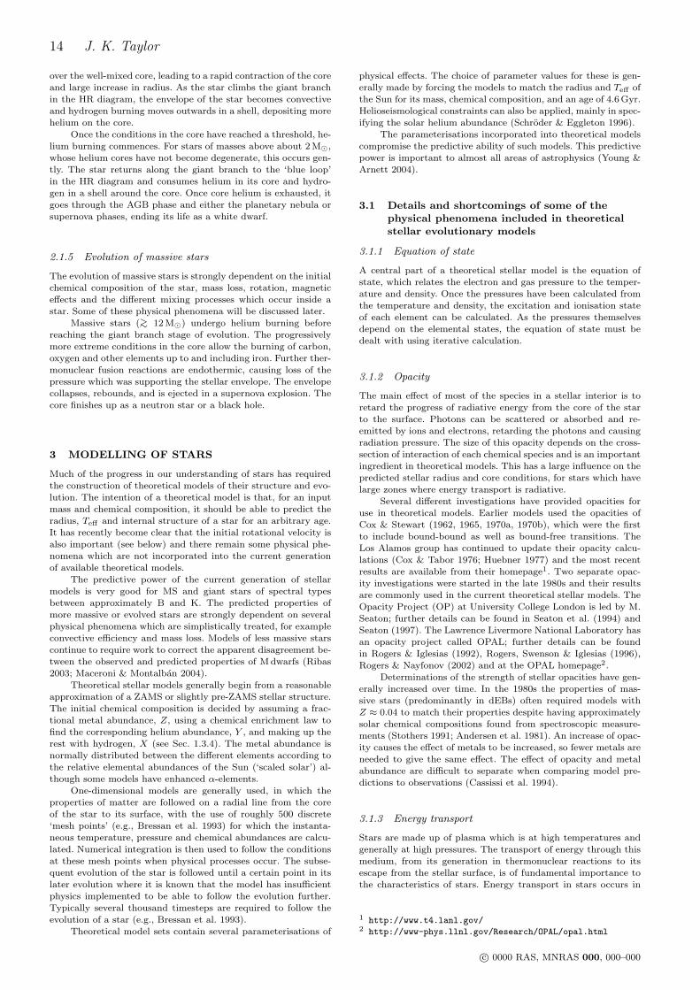
14 J. K. Taylor
over the well-mixed core, leading to a rapid contraction of the coreand large increase in radius. As the star climbs the giant branchin the HR diagram, the envelope of the star becomes convectiveand hydrogen burning moves outwards in a shell, depositing morehelium on the core.
Once the conditions in the core have reached a threshold, he-lium burning commences. For stars of masses above about 2 M¯,whose helium cores have not become degenerate, this occurs gen-tly. The star returns along the giant branch to the ‘blue loop’in the HR diagram and consumes helium in its core and hydro-gen in a shell around the core. Once core helium is exhausted, itgoes through the AGB phase and either the planetary nebula orsupernova phases, ending its life as a white dwarf.
2.1.5 Evolution of massive stars
The evolution of massive stars is strongly dependent on the initialchemical composition of the star, mass loss, rotation, magneticeffects and the different mixing processes which occur inside astar. Some of these physical phenomena will be discussed later.
Massive stars (>∼ 12 M¯) undergo helium burning beforereaching the giant branch stage of evolution. The progressivelymore extreme conditions in the core allow the burning of carbon,oxygen and other elements up to and including iron. Further ther-monuclear fusion reactions are endothermic, causing loss of thepressure which was supporting the stellar envelope. The envelopecollapses, rebounds, and is ejected in a supernova explosion. Thecore finishes up as a neutron star or a black hole.
3 MODELLING OF STARS
Much of the progress in our understanding of stars has requiredthe construction of theoretical models of their structure and evo-lution. The intention of a theoretical model is that, for an inputmass and chemical composition, it should be able to predict theradius, Teff and internal structure of a star for an arbitrary age.It has recently become clear that the initial rotational velocity isalso important (see below) and there remain some physical phe-nomena which are not incorporated into the current generationof available theoretical models.
The predictive power of the current generation of stellarmodels is very good for MS and giant stars of spectral typesbetween approximately B and K. The predicted properties ofmore massive or evolved stars are strongly dependent on severalphysical phenomena which are simplistically treated, for exampleconvective efficiency and mass loss. Models of less massive starscontinue to require work to correct the apparent disagreement be-tween the observed and predicted properties of M dwarfs (Ribas2003; Maceroni & Montalban 2004).
Theoretical stellar models generally begin from a reasonableapproximation of a ZAMS or slightly pre-ZAMS stellar structure.The initial chemical composition is decided by assuming a frac-tional metal abundance, Z, using a chemical enrichment law tofind the corresponding helium abundance, Y , and making up therest with hydrogen, X (see Sec. 1.3.4). The metal abundance isnormally distributed between the different elements according tothe relative elemental abundances of the Sun (‘scaled solar’) al-though some models have enhanced α-elements.
One-dimensional models are generally used, in which theproperties of matter are followed on a radial line from the coreof the star to its surface, with the use of roughly 500 discrete‘mesh points’ (e.g., Bressan et al. 1993) for which the instanta-neous temperature, pressure and chemical abundances are calcu-lated. Numerical integration is then used to follow the conditionsat these mesh points when physical processes occur. The subse-quent evolution of the star is followed until a certain point in itslater evolution where it is known that the model has insufficientphysics implemented to be able to follow the evolution further.Typically several thousand timesteps are required to follow theevolution of a star (e.g., Bressan et al. 1993).
Theoretical model sets contain several parameterisations of
physical effects. The choice of parameter values for these is gen-erally made by forcing the models to match the radius and Teff ofthe Sun for its mass, chemical composition, and an age of 4.6 Gyr.Helioseismological constraints can also be applied, mainly in spec-ifying the solar helium abundance (Schroder & Eggleton 1996).
The parameterisations incorporated into theoretical modelscompromise the predictive ability of such models. This predictivepower is important to almost all areas of astrophysics (Young &Arnett 2004).
3.1 Details and shortcomings of some of thephysical phenomena included in theoreticalstellar evolutionary models
3.1.1 Equation of state
A central part of a theoretical stellar model is the equation ofstate, which relates the electron and gas pressure to the temper-ature and density. Once the pressures have been calculated fromthe temperature and density, the excitation and ionisation stateof each element can be calculated. As the pressures themselvesdepend on the elemental states, the equation of state must bedealt with using iterative calculation.
3.1.2 Opacity
The main effect of most of the species in a stellar interior is toretard the progress of radiative energy from the core of the starto the surface. Photons can be scattered or absorbed and re-emitted by ions and electrons, retarding the photons and causingradiation pressure. The size of this opacity depends on the cross-section of interaction of each chemical species and is an importantingredient in theoretical models. This has a large influence on thepredicted stellar radius and core conditions, for stars which havelarge zones where energy transport is radiative.
Several different investigations have provided opacities foruse in theoretical models. Earlier models used the opacities ofCox & Stewart (1962, 1965, 1970a, 1970b), which were the firstto include bound-bound as well as bound-free transitions. TheLos Alamos group has continued to update their opacity calcu-lations (Cox & Tabor 1976; Huebner 1977) and the most recentresults are available from their homepage1. Two separate opac-ity investigations were started in the late 1980s and their resultsare commonly used in the current theoretical stellar models. TheOpacity Project (OP) at University College London is led by M.Seaton; further details can be found in Seaton et al. (1994) andSeaton (1997). The Lawrence Livermore National Laboratory hasan opacity project called OPAL; further details can be foundin Rogers & Iglesias (1992), Rogers, Swenson & Iglesias (1996),Rogers & Nayfonov (2002) and at the OPAL homepage2.
Determinations of the strength of stellar opacities have gen-erally increased over time. In the 1980s the properties of mas-sive stars (predominantly in dEBs) often required models withZ ≈ 0.04 to match their properties despite having approximatelysolar chemical compositions found from spectroscopic measure-ments (Stothers 1991; Andersen et al. 1981). An increase of opac-ity causes the effect of metals to be increased, so fewer metals areneeded to give the same effect. The effect of opacity and metalabundance are difficult to separate when comparing model pre-dictions to observations (Cassissi et al. 1994).
3.1.3 Energy transport
Stars are made up of plasma which is at high temperatures andgenerally at high pressures. The transport of energy through thismedium, from its generation in thermonuclear reactions to itsescape from the stellar surface, is of fundamental importance tothe characteristics of stars. Energy transport in stars occurs in
1 http://www.t4.lanl.gov/2 http://www-phys.llnl.gov/Research/OPAL/opal.html
c© 0000 RAS, MNRAS 000, 000–000
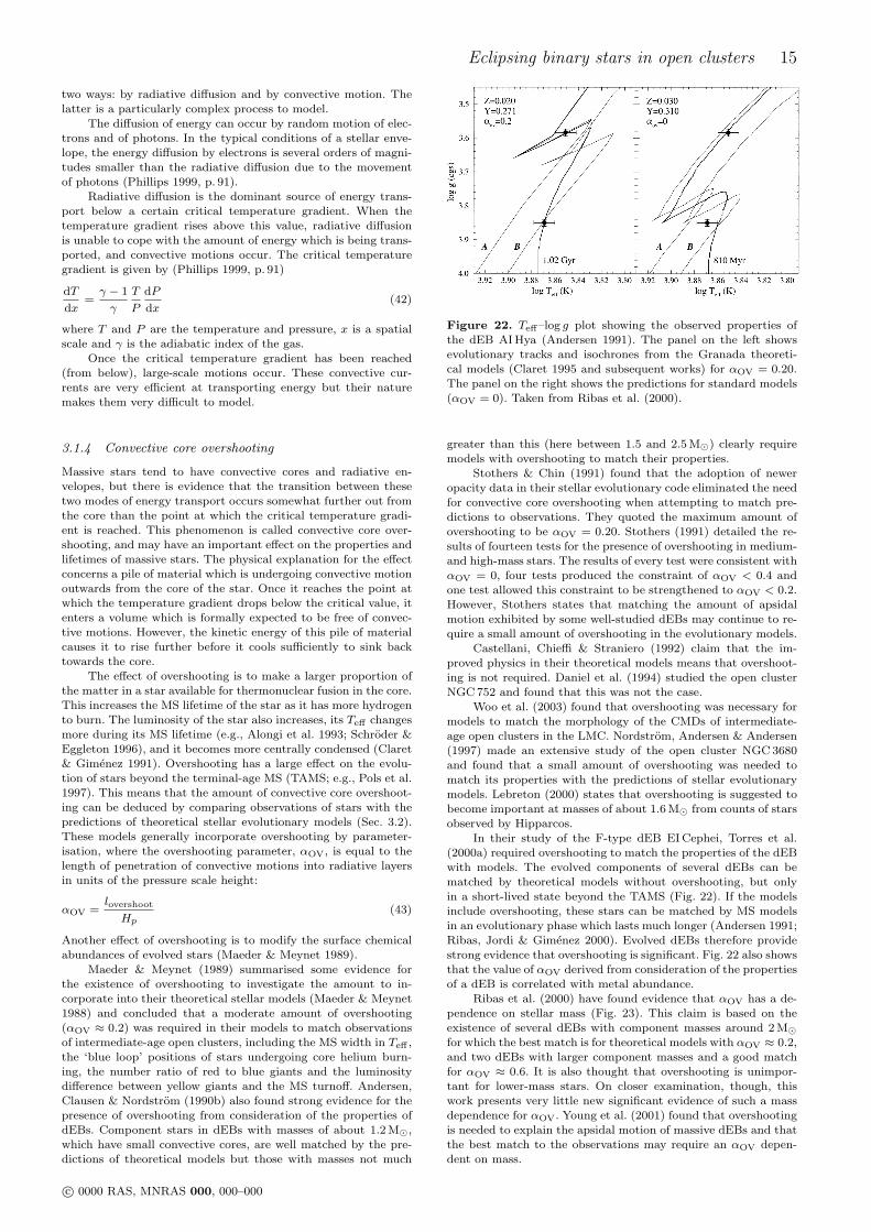
Eclipsing binary stars in open clusters 15
two ways: by radiative diffusion and by convective motion. Thelatter is a particularly complex process to model.
The diffusion of energy can occur by random motion of elec-trons and of photons. In the typical conditions of a stellar enve-lope, the energy diffusion by electrons is several orders of magni-tudes smaller than the radiative diffusion due to the movementof photons (Phillips 1999, p. 91).
Radiative diffusion is the dominant source of energy trans-port below a certain critical temperature gradient. When thetemperature gradient rises above this value, radiative diffusionis unable to cope with the amount of energy which is being trans-ported, and convective motions occur. The critical temperaturegradient is given by (Phillips 1999, p. 91)
dT
dx=γ − 1
γ
T
P
dP
dx(42)
where T and P are the temperature and pressure, x is a spatialscale and γ is the adiabatic index of the gas.
Once the critical temperature gradient has been reached(from below), large-scale motions occur. These convective cur-rents are very efficient at transporting energy but their naturemakes them very difficult to model.
3.1.4 Convective core overshooting
Massive stars tend to have convective cores and radiative en-velopes, but there is evidence that the transition between thesetwo modes of energy transport occurs somewhat further out fromthe core than the point at which the critical temperature gradi-ent is reached. This phenomenon is called convective core over-shooting, and may have an important effect on the properties andlifetimes of massive stars. The physical explanation for the effectconcerns a pile of material which is undergoing convective motionoutwards from the core of the star. Once it reaches the point atwhich the temperature gradient drops below the critical value, itenters a volume which is formally expected to be free of convec-tive motions. However, the kinetic energy of this pile of materialcauses it to rise further before it cools sufficiently to sink backtowards the core.
The effect of overshooting is to make a larger proportion ofthe matter in a star available for thermonuclear fusion in the core.This increases the MS lifetime of the star as it has more hydrogento burn. The luminosity of the star also increases, its Teff changesmore during its MS lifetime (e.g., Alongi et al. 1993; Schroder &Eggleton 1996), and it becomes more centrally condensed (Claret& Gimenez 1991). Overshooting has a large effect on the evolu-tion of stars beyond the terminal-age MS (TAMS; e.g., Pols et al.1997). This means that the amount of convective core overshoot-ing can be deduced by comparing observations of stars with thepredictions of theoretical stellar evolutionary models (Sec. 3.2).These models generally incorporate overshooting by parameter-isation, where the overshooting parameter, αOV, is equal to thelength of penetration of convective motions into radiative layersin units of the pressure scale height:
αOV =lovershoot
Hp(43)
Another effect of overshooting is to modify the surface chemicalabundances of evolved stars (Maeder & Meynet 1989).
Maeder & Meynet (1989) summarised some evidence forthe existence of overshooting to investigate the amount to in-corporate into their theoretical stellar models (Maeder & Meynet1988) and concluded that a moderate amount of overshooting(αOV ≈ 0.2) was required in their models to match observationsof intermediate-age open clusters, including the MS width in Teff ,the ‘blue loop’ positions of stars undergoing core helium burn-ing, the number ratio of red to blue giants and the luminositydifference between yellow giants and the MS turnoff. Andersen,Clausen & Nordstrom (1990b) also found strong evidence for thepresence of overshooting from consideration of the properties ofdEBs. Component stars in dEBs with masses of about 1.2 M¯,which have small convective cores, are well matched by the pre-dictions of theoretical models but those with masses not much
Figure 22. Teff–log g plot showing the observed properties ofthe dEB AI Hya (Andersen 1991). The panel on the left showsevolutionary tracks and isochrones from the Granada theoreti-cal models (Claret 1995 and subsequent works) for αOV = 0.20.The panel on the right shows the predictions for standard models(αOV = 0). Taken from Ribas et al. (2000).
greater than this (here between 1.5 and 2.5 M¯) clearly requiremodels with overshooting to match their properties.
Stothers & Chin (1991) found that the adoption of neweropacity data in their stellar evolutionary code eliminated the needfor convective core overshooting when attempting to match pre-dictions to observations. They quoted the maximum amount ofovershooting to be αOV = 0.20. Stothers (1991) detailed the re-sults of fourteen tests for the presence of overshooting in medium-and high-mass stars. The results of every test were consistent withαOV = 0, four tests produced the constraint of αOV < 0.4 andone test allowed this constraint to be strengthened to αOV < 0.2.However, Stothers states that matching the amount of apsidalmotion exhibited by some well-studied dEBs may continue to re-quire a small amount of overshooting in the evolutionary models.
Castellani, Chieffi & Straniero (1992) claim that the im-proved physics in their theoretical models means that overshoot-ing is not required. Daniel et al. (1994) studied the open clusterNGC 752 and found that this was not the case.
Woo et al. (2003) found that overshooting was necessary formodels to match the morphology of the CMDs of intermediate-age open clusters in the LMC. Nordstrom, Andersen & Andersen(1997) made an extensive study of the open cluster NGC 3680and found that a small amount of overshooting was needed tomatch its properties with the predictions of stellar evolutionarymodels. Lebreton (2000) states that overshooting is suggested tobecome important at masses of about 1.6 M¯ from counts of starsobserved by Hipparcos.
In their study of the F-type dEB EI Cephei, Torres et al.(2000a) required overshooting to match the properties of the dEBwith models. The evolved components of several dEBs can bematched by theoretical models without overshooting, but onlyin a short-lived state beyond the TAMS (Fig. 22). If the modelsinclude overshooting, these stars can be matched by MS modelsin an evolutionary phase which lasts much longer (Andersen 1991;Ribas, Jordi & Gimenez 2000). Evolved dEBs therefore providestrong evidence that overshooting is significant. Fig. 22 also showsthat the value of αOV derived from consideration of the propertiesof a dEB is correlated with metal abundance.
Ribas et al. (2000) have found evidence that αOV has a de-pendence on stellar mass (Fig. 23). This claim is based on theexistence of several dEBs with component masses around 2 M¯for which the best match is for theoretical models with αOV ≈ 0.2,and two dEBs with larger component masses and a good matchfor αOV ≈ 0.6. It is also thought that overshooting is unimpor-tant for lower-mass stars. On closer examination, though, thiswork presents very little new significant evidence of such a massdependence for αOV. Young et al. (2001) found that overshootingis needed to explain the apsidal motion of massive dEBs and thatthe best match to the observations may require an αOV depen-dent on mass.
c© 0000 RAS, MNRAS 000, 000–000
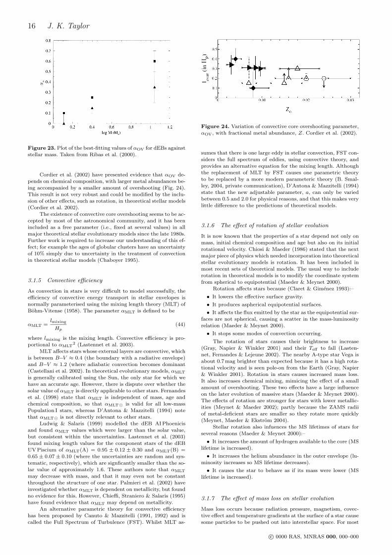
16 J. K. Taylor
Figure 23. Plot of the best-fitting values of αOV for dEBs againststellar mass. Taken from Ribas et al. (2000).
Cordier et al. (2002) have presented evidence that αOV de-pends on chemical composition, with larger metal abundances be-ing accompanied by a smaller amount of overshooting (Fig. 24).This result is not very robust and could be modified by the inclu-sion of other effects, such as rotation, in theoretical stellar models(Cordier et al. 2002).
The existence of convective core overshooting seems to be ac-cepted by most of the astronomical community, and it has beenincluded as a free parameter (i.e., fixed at several values) in allmajor theoretical stellar evolutionary models since the late 1980s.Further work is required to increase our understanding of this ef-fect; for example the ages of globular clusters have an uncertaintyof 10% simply due to uncertainty in the treatment of convectionin theoretical stellar models (Chaboyer 1995).
3.1.5 Convective efficiency
As convection in stars is very difficult to model successfully, theefficiency of convective energy transport in stellar envelopes isnormally parameterised using the mixing length theory (MLT) ofBohm-Vitense (1958). The parameter αMLT is defined to be
αMLT =lmixing
Hp(44)
where lmixing is the mixing length. Convective efficiency is pro-portional to αMLT
2 (Lastennet et al. 2003).
MLT affects stars whose external layers are convective, whichis between B−V ≈ 0.4 (the boundary with a radiative envelope)and B−V ≈ 1.2 (where adiabatic convection becomes dominant(Castellani et al. 2002). In theoretical evolutionary models, αMLT
is generally calibrated using the Sun, the only star for which wehave an accurate age. However, there is dispute over whether thesolar value of αMLT is directly applicable to other stars. Fernandeset al. (1998) state that αMLT is independent of mass, age andchemical composition, so that αMLT¯ is valid for all low-massPopulation I stars, whereas D’Antona & Mazzitelli (1994) notethat αMLT¯ is not directly relevant to other stars.
Ludwig & Salaris (1999) modelled the dEB AI Phoenicisand found αMLT values which were larger than the solar value,but consistent within the uncertainties. Lastennet et al. (2003)found mixing length values for the component stars of the dEBUV Piscium of αMLT(A) = 0.95 ± 0.12 ± 0.30 and αMLT(B) =0.65 ± 0.07 ± 0.10 (where the uncertainties are random and sys-tematic, respectively), which are signficantly smaller than the so-lar value of approximately 1.6. These authors note that αMLT
may decrease with mass, and that it may even not be constantthroughout the structure of one star. Palmieri et al. (2002) haveinvestigated whether αMLT is dependent on metallicity, but foundno evidence for this. However, Chieffi, Straniero & Salaris (1995)have found evidence that αMLT may depend on metallicity.
An alternative parametric theory for convective efficiencyhas been proposed by Canuto & Mazzitelli (1991, 1992) and iscalled the Full Spectrum of Turbulence (FST). Whilst MLT as-
Figure 24. Variation of convective core overshooting parameter,αOV, with fractional metal abundance, Z. Cordier et al. (2002).
sumes that there is one large eddy in stellar convection, FST con-siders the full spectrum of eddies, using convective theory, andprovides an alternative equation for the mixing length. Althoughthe replacement of MLT by FST causes one parametric theoryto be replaced by a more modern parameteric theory (B. Smal-ley, 2004, private communication), D’Antona & Mazzitelli (1994)state that the new adjustable parameter, a, can only be variedbetween 0.5 and 2.0 for physical reasons, and that this makes verylittle difference to the predictions of theoretical models.
3.1.6 The effect of rotation of stellar evolution
It is now known that the properties of a star depend not only onmass, initial chemical composition and age but also on its initialrotational velocity. Chiosi & Maeder (1986) stated that the nextmajor piece of physics which needed incorporation into theoreticalstellar evolutionary models is rotation. It has been included inmost recent sets of theoretical models. The usual way to includerotation in theoretical models is to modify the coordinate systemfrom spherical to equipotential (Maeder & Meynet 2000).
Rotation affects stars because (Claret & Gimenez 1993):–
• It lowers the effective surface gravity.
• It produces aspherical equipotential surfaces.
• It affects the flux emitted by the star as the equipotential sur-faces are not spherical, causing a scatter in the mass-luminosityrelation (Maeder & Meynet 2000).
• It stops some modes of convection occurring.
The rotation of stars causes their brightness to increase(Gray, Napier & Winkler 2001) and their Teff to fall (Lasten-net, Fernandes & Lejeune 2002). The nearby A-type star Vega isabout 0.7 mag brighter than expected because it has a high rota-tional velocity and is seen pole-on from the Earth (Gray, Napier& Winkler 2001). Rotation in stars causes increased mass loss.It also increases chemical mixing, mimicing the effect of a smallamount of overshooting. These two effects have a large influenceon the later evolution of massive stars (Maeder & Meynet 2000).The effects of rotation are stronger for stars with lower metallic-ities (Meynet & Maeder 2002); partly because the ZAMS radiiof metal-deficient stars are smaller so they rotate more quickly(Meynet, Maeder & Ekstrom 2004).
Stellar rotation also infuences the MS lifetimes of stars forseveral reasons (Maeder & Meynet 2000):–
• It increases the amount of hydrogen available to the core (MSlifetime is increased).
• It increases the helium abundance in the outer envelope (lu-minosity increases so MS lifetime decreases).
• It causes the star to behave as if its mass were lower (MSlifetime is increased).
3.1.7 The effect of mass loss on stellar evolution
Mass loss occurs because radiation pressure, magnetism, covec-tive effect and temperature gradients at the surface of a star causesome particles to be pushed out into interstellar space. For most
c© 0000 RAS, MNRAS 000, 000–000
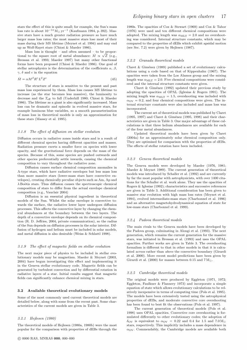
Eclipsing binary stars in open clusters 17
stars the effect of this is quite small; for example, the Sun’s massloss rate is about 10−14 M¯ yr−1 (Kaufmann 1994, p. 392). Mas-sive stars have a much greater radiation pressure so have muchlarger mass loss rates; the most massive stars lose most of theirmass during their MS lifetime (Meynet et al. 1994) and may endup as Wolf-Rayet stars (Chiosi & Maeder 1986).
Mass loss is thought – and often assumed – to be propor-tional to the square root of metal abundance: M ∝
√Z (e.g.,
Bressan et al. 1993; Maeder 1997) but many other functionalforms have been proposed (Chiosi & Maeder 1986). One goal ofstellar astrophysics is the determination of the coefficients α, β,γ, δ and ε in the equation
M = αMβRγLδZε (45)
The structure of stars is sensitive to the present and pastmass loss experienced by them. Mass loss causes MS lifetime toincrease (as the star becomes less massive), the luminosity todecrease and the Teff to fall (Underhill 1980; Chiosi & Maeder1986). The lifetime as a giant is also significantly increased. Massloss can be dramatic and episodic in evolved massive stars, forexample luminous blue variables, so a smooth parameterisationof mass loss in theoretical models is only an approximation forthese stars (Massey et al. 1995).
3.1.8 The effect of diffusion on stellar evolution
Diffusion occurs in radiative zones inside stars and is a result ofdifferent chemical species having different opacities and masses.Radiation pressure exerts a smaller force on species with loweropacity, and the gravitational force depends on the mass of thespecies. Because of this, some species are pushed outwards andother species preferentially settle inwards, causing the chemicalcomposition to vary throughout the radiative zone.
Diffusion causes surface chemical composition anomalies inA-type stars, which have radiative envelopes but less mass lossthan more massive stars (lower-mass stars have convective en-velopes), creating chemically peculiar objects such as Am, Ap andλBootis stars. Thus diffusion causes the spectroscopic chemicalcomposition of stars to differ from the actual envelope chemicalcomposition (e.g., Vauclair 2004)
Diffusion is an essential physical ingredient in theoreticalmodels of the Sun. Whilst the solar envelope is convective to-wards the surface, the radiative lower layer undergoes diffusionprocesses. This affects the convective layer by changing the chem-ical abundances at the boundary between the two layers. Thedepth of a convective envelope depends on its chemical composi-tion (R. D. Jeffries, 2004, private communication), so the radiusof the Sun depends on diffusion processes in the solar interior. Dif-fusion of hydrogen and helium must be included in solar models,and metal diffusion is also desirable (Weiss & Schlattl 1998).
3.1.9 The effect of magnetic fields on stellar evolution
The next major piece of physics to be included in stellar evo-lutionary models may be magnetism. Maeder & Meynet (2003,2004) have begun investigating this effect and implementing itin the Geneva stellar evolutionary code. Magnetic fields can begenerated by turbulent convection and by differential rotation inradiative layers of a star. Initial results suggest that magneticfields can significantly enhance chemical mixing in stars.
3.2 Available theoretical evolutionary models
Some of the most commonly used current theoretical models aredetailed below, along with some from the recent past. Some char-acteristics of the current models are given in Table 3.
3.2.1 Hejlesen (1980)
The theoretical models of Hejlesen (1980a, 1980b) were the mostpopular for the comparison with properties of dEBs through the
1980s. The opacities of Cox & Stewart (1969) and Cox & Tabor(1976) were used and ten different chemical compositions wereadopted. The mixing length was αMLT = 2.0 and no overshoot-ing was considered. Internal structure constants, which may becompared to the properties of dEBs which exhibit apsidal motion(see Sec. 7.2) were given by Hejlesen (1987).
3.2.2 Granada theoretical models
Claret & Gimenez (1989) published a set of evolutionary calcu-lations using a code based on that of Kippenhahn (1967). Theopacities were taken from the Los Alamos group and the mixinglength was αMLT = 2.0. Five chemical compositions were consid-ered and the internal structure constants were given.
Claret & Gimenez (1992) updated their previous study byadopting the opacities of OPAL (Iglesias & Rogers 1991). Themixing length was αMLT = 1.5, overshooting was included withαOV = 0.2, and four chemical compositions were given. The in-ternal structure constants were also included and mass loss wasincorporated.
The current set of theoretical models was published by Claret(1995, 1997) and Claret & Gimenez (1995, 1998) and their char-acteristics are given in Table 3. One major advantage of these cal-culations is that three helium abundances are available for eachof the four metal abundances.
Updated theoretical models have been given by Claret(2004a) for an approximately solar chemical composition only.They are optimised for comparison with the properties of dEBs.The effects of stellar rotation have been included.
3.2.3 Geneva theoretical models
The Geneva models were developed by Maeder (1976, 1981;Maeder & Meynet 1989). The current generation of theoreticalmodels was introduced by Schaller et al. (1992) and are currentlyby far the most popular with astrophysicists, with over 1400 cita-tions for the Schaller et al. work alone. They use the opacities ofRogers & Iglesias (1992); characteristics and successive referencesare given in Table 3. Additional consideration has been given tomassive star evolution with high mass loss rates (Meynet et al.1994), evolved intermediate-mass stars (Charbonnel et al. 1996)and an alternative magnetohydrodynamical equation of state forlow-mass stars (Charbonnel et al. 1999).
3.2.4 Padova theoretical models
The main rivals to the Geneva models have been developed bythe Padova group, culminating in Alongi et al. (1993). The nextgeneration, which remains the current generation for the massivestars, was initiated in Bressan et al. (1993) and uses the OPALopacities. Further works are given in Table 3. The overshootingformalism is different to that in other models in that it is calcu-lated across rather than above the convective boundary (Girardiet al. 2000). More recent model predictions have been given byGirardi et al. (2000) for masses between 0.15 and 7 M¯.
3.2.5 Cambridge theoretical models
The original models were produced by Eggleton (1971, 1972;Eggleton, Faulkner & Flannery 1973) and incorporate a simpleequation of state which allows evolutionary calculations to be rel-atively inexpensive in terms of computing time (Pols et al. 1995).The models have been extensively tested using the astrophysicalproperties of dEBs, and moderate convective core overshootinghas been found to best fit the observations (Pols et al. 1997).
The current generation of theoretical models (Pols et al.1998) uses OPAL opacities. Convective core overshooting is for-mulated differently to other evolutionary codes; the adoption ofδOV is equivalent to αOV = 0.22 and 0.4 for 1.5 and 7.0 M¯stars, respectively. This implicitly includes a mass dependence inαOV. Commendably, the Cambridge models are available both
c© 0000 RAS, MNRAS 000, 000–000
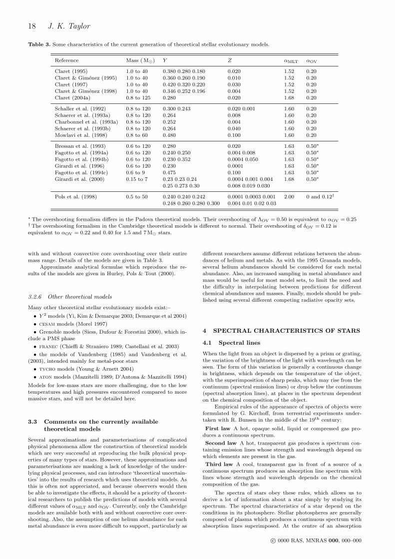
18 J. K. Taylor
Table 3. Some characteristics of the current generation of theoretical stellar evolutionary models.
Reference Mass ( M¯) Y Z αMLT αOV
Claret (1995) 1.0 to 40 0.380 0.280 0.180 0.020 1.52 0.20Claret & Gimenez (1995) 1.0 to 40 0.360 0.260 0.190 0.010 1.52 0.20Claret (1997) 1.0 to 40 0.420 0.320 0.220 0.030 1.52 0.20Claret & Gimenez (1998) 1.0 to 40 0.346 0.252 0.196 0.004 1.52 0.20Claret (2004a) 0.8 to 125 0.280 0.020 1.68 0.20
Schaller et al. (1992) 0.8 to 120 0.300 0.243 0.020 0.001 1.60 0.20Schaerer et al. (1993a) 0.8 to 120 0.264 0.008 1.60 0.20Charbonnel et al. (1993a) 0.8 to 120 0.252 0.004 1.60 0.20Schaerer et al. (1993b) 0.8 to 120 0.264 0.040 1.60 0.20Mowlavi et al. (1998) 0.8 to 60 0.480 0.100 1.60 0.20
Bressan et al. (1993) 0.6 to 120 0.280 0.020 1.63 0.50∗
Fagotto et al. (1994a) 0.6 to 120 0.240 0.250 0.004 0.008 1.63 0.50∗
Fagotto et al. (1994b) 0.6 to 120 0.230 0.352 0.0004 0.050 1.63 0.50∗
Girardi et al. (1996) 0.6 to 120 0.230 0.0001 1.63 0.50∗
Fagotto et al. (1994c) 0.6 to 9 0.475 0.100 1.63 0.50∗
Girardi et al. (2000) 0.15 to 7 0.23 0.23 0.24 0.0004 0.001 0.004 1.68 0.50∗
0.25 0.273 0.30 0.008 0.019 0.030
Pols et al. (1998) 0.5 to 50 0.240 0.240 0.242 0.0001 0.0003 0.001 2.00 0 and 0.12†
0.248 0.260 0.280 0.300 0.004 0.01 0.02 0.03
∗ The overshooting formalism differs in the Padova theoretical models. Their overshooting of ΛOV = 0.50 is equivalent to αOV = 0.25† The overshooting formalism in the Cambridge theoretical models is different to normal. Their overshooting of δOV = 0.12 isequivalent to αOV = 0.22 and 0.40 for 1.5 and 7 M¯ stars.
with and without convective core overshooting over their entiremass range. Details of the models are given in Table 3.
Approximate analytical formulae which reproduce the re-sults of the models are given in Hurley, Pols & Tout (2000).
3.2.6 Other theoretical models
Many other theoretical stellar evolutionary models exist:–
• Y 2 models (Yi, Kim & Demarque 2003; Demarque et al 2004)
• cesam models (Morel 1997)
• Grenoble models (Siess, Dufour & Forestini 2000), which in-clude a PMS phase
• franec (Chieffi & Straniero 1989; Castellani et al. 2003)
• the models of Vandenberg (1985) and Vandenberg et al.(2003), intended mainly for metal-poor stars
• tycho models (Young & Arnett 2004)
• aton models (Mazzitelli 1989; D’Antona & Mazzitelli 1994)
Models for low-mass stars are more challenging, due to the lowtemperatures and high pressures encountered compared to moremassive stars, and will not be detailed here.
3.3 Comments on the currently availabletheoretical models
Several approximations and parameterisations of complicatedphysical phenomena allow the construction of theoretical modelswhich are very successful at reproducing the bulk physical prop-erties of many types of stars. However, these approximations andparameterisations are masking a lack of knowledge of the under-lying physical processes, and can introduce ‘theoretical uncertain-ties’ into the results of research which uses theoretical models. Asthis is often not appreciated, and because observers would thenbe able to investigate the effects, it should be a priority of theoret-ical researchers to publish the predictions of models with severaldifferent values of αMLT and αOV. Currently, only the Cambridgemodels are available both with and without convective core over-shooting. Also, the assumption of one helium abundance for eachmetal abundance is even more difficult to support, particularly as
different researchers assume different relations between the abun-dances of helium and metals. As with the 1995 Granada models,several helium abundances should be considered for each metalabundance. Also, an increased sampling in metal abundance andmass would be useful for most model sets, to limit the need andthe difficulty in interpolating between predictions for differentchemical abundances and masses. Finally, models should be pub-lished using several different competing radiative opacity sets.
4 SPECTRAL CHARACTERISTICS OF STARS
4.1 Spectral lines
When the light from an object is dispersed by a prism or grating,the variation of the brightness of the light with wavelength can beseen. The form of this variation is generally a continuous changein brightness, which depends on the temperature of the object,with the superimposition of sharp peaks, which may rise from thecontinuum (spectral emission lines) or drop below the continuum(spectral absorption lines), at places in the spectrum dependenton the chemical composition of the object.
Empirical rules of the appearance of spectra of objects wereformulated by G. Kirchoff, from terrestrial experiments under-taken with R. Bunsen in the middle of the 19th century:
First law A hot, opaque solid, liquid or compressed gas pro-duces a continuous spectrum.
Second law A hot, transparent gas produces a spectrum con-taining emission lines whose strength and wavelength depend onwhich elements are present in the gas.
Third law A cool, transparent gas in front of a source of acontinuous spectrum produces an absorption line spectrum withlines whose strength and wavelength depends on the chemicalcomposition of the gas.
The spectra of stars obey these rules, which allows us toderive a lot of information about a star simply by studying itsspectrum. The spectral characteristics of a star depend on theconditions in its photosphere. Stellar photospheres are generallycomposed of plasma which produces a continuous spectrum withabsorption lines superimposed. At the centre of an absorption
c© 0000 RAS, MNRAS 000, 000–000
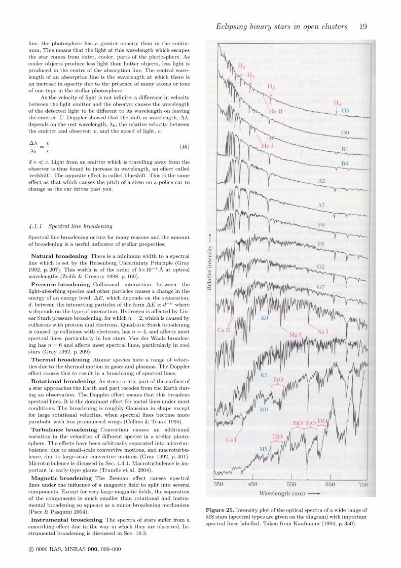
Eclipsing binary stars in open clusters 19
line, the photosphere has a greater opacity than in the contin-uum. This means that the light at this wavelength which escapesthe star comes from outer, cooler, parts of the photosphere. Ascooler objects produce less light than hotter objects, less light isproduced in the centre of the absorption line. The central wave-length of an absorption line is the wavelength at which there isan increase in opacity due to the presence of many atoms or ionsof one type in the stellar photosphere.
As the velocity of light is not infinite, a difference in velocitybetween the light emitter and the observer causes the wavelengthof the detected light to be different to its wavelength on leavingthe emitter. C. Doppler showed that the shift in wavelength, ∆λ,depends on the rest wavelength, λ0, the relative velocity betweenthe emitter and observer, v, and the speed of light, c:
∆λ
λ0=v
c(46)
if v ¿ c. Light from an emitter which is travelling away from theobserver is thus found to increase in wavelength, an effect called‘redshift’. The opposite effect is called blueshift. This is the sameeffect as that which causes the pitch of a siren on a police car tochange as the car drives past you.
4.1.1 Spectral line broadening
Spectral line broadening occurs for many reasons and the amountof broadening is a useful indicator of stellar properties.
Natural broadening There is a minimum width to a spectralline which is set by the Heisenberg Uncertainty Principle (Gray1992, p. 207). This width is of the order of 5×10⁻⁴ A at opticalwavelengths (Zeilik & Gregory 1998, p. 169).
Pressure broadening Collisional interaction between thelight-absorbing species and other particles causes a change in theenergy of an energy level, ∆E, which depends on the separation,d, between the interacting particles of the form ∆E ∝ d−n wheren depends on the type of interaction. Hydrogen is affected by Lin-ear Stark pressure broadening, for which n = 2, which is caused bycollisions with protons and electrons. Quadratic Stark broadeningis caused by collisions with electrons, has n = 4, and affects mostspectral lines, particularly in hot stars. Van der Waals broaden-ing has n = 6 and affects most spectral lines, particularly in coolstars (Gray 1992, p. 209).
Thermal broadening Atomic species have a range of veloci-ties due to the thermal motion in gases and plasmas. The Dopplereffect causes this to result in a broadening of spectral lines.
Rotational broadening As stars rotate, part of the surface ofa star approaches the Earth and part recedes from the Earth dur-ing an observation. The Doppler effect means that this broadensspectral lines. It is the dominant effect for metal lines under mostconditions. The broadening is roughly Gaussian in shape exceptfor large rotational velocites, when spectral lines become moreparabolic with less pronounced wings (Collins & Truax 1995).
Turbulence broadening Convection causes an additionalvariation in the velocities of different species in a stellar photo-sphere. The effects have been arbitrarily separated into microtur-bulence, due to small-scale convective motions, and macroturbu-lence, due to large-scale convective motions (Gray 1992, p. 401).Microturbulence is dicussed in Sec. 4.4.1. Macroturbulence is im-portant in early-type giants (Trundle et al. 2004).
Magnetic broadening The Zeeman effect causes spectrallines under the influence of a magnetic field to split into severalcomponents. Except for very large magnetic fields, the separationof the components is much smaller than rotational and instru-mental broadening so appears as a minor broadening mechanism(Pace & Pasquini 2004).
Instrumental broadening The spectra of stars suffer from asmoothing effect due to the way in which they are observed. In-strumental broadening is discussed in Sec. 10.3.
Figure 25. Intensity plot of the optical spectra of a wide range ofMS stars (spectral types are given on the diagram) with importantspectral lines labelled. Taken from Kaufmann (1994, p. 350).
c© 0000 RAS, MNRAS 000, 000–000
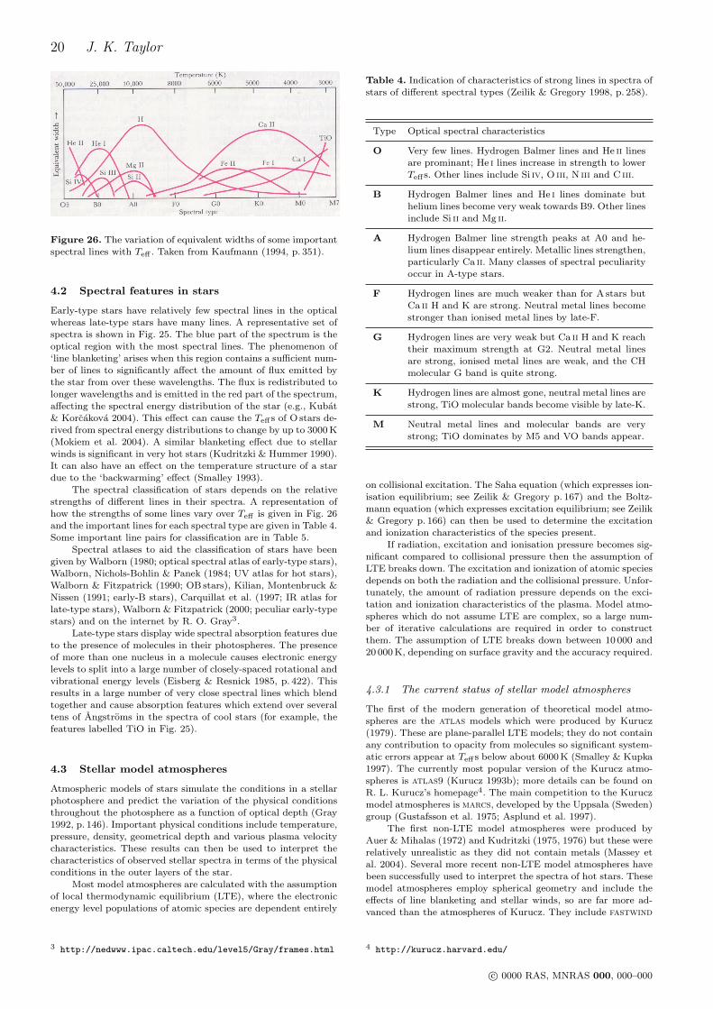
20 J. K. Taylor
Figure 26. The variation of equivalent widths of some importantspectral lines with Teff . Taken from Kaufmann (1994, p. 351).
4.2 Spectral features in stars
Early-type stars have relatively few spectral lines in the opticalwhereas late-type stars have many lines. A representative set ofspectra is shown in Fig. 25. The blue part of the spectrum is theoptical region with the most spectral lines. The phenomenon of‘line blanketing’ arises when this region contains a sufficient num-ber of lines to significantly affect the amount of flux emitted bythe star from over these wavelengths. The flux is redistributed tolonger wavelengths and is emitted in the red part of the spectrum,affecting the spectral energy distribution of the star (e.g., Kubat& Korcakova 2004). This effect can cause the Teffs of O stars de-rived from spectral energy distributions to change by up to 3000 K(Mokiem et al. 2004). A similar blanketing effect due to stellarwinds is significant in very hot stars (Kudritzki & Hummer 1990).It can also have an effect on the temperature structure of a stardue to the ‘backwarming’ effect (Smalley 1993).
The spectral classification of stars depends on the relativestrengths of different lines in their spectra. A representation ofhow the strengths of some lines vary over Teff is given in Fig. 26and the important lines for each spectral type are given in Table 4.Some important line pairs for classification are in Table 5.
Spectral atlases to aid the classification of stars have beengiven by Walborn (1980; optical spectral atlas of early-type stars),Walborn, Nichols-Bohlin & Panek (1984; UV atlas for hot stars),Walborn & Fitzpatrick (1990; OB stars), Kilian, Montenbruck &Nissen (1991; early-B stars), Carquillat et al. (1997; IR atlas forlate-type stars), Walborn & Fitzpatrick (2000; peculiar early-typestars) and on the internet by R. O. Gray3.
Late-type stars display wide spectral absorption features dueto the presence of molecules in their photospheres. The presenceof more than one nucleus in a molecule causes electronic energylevels to split into a large number of closely-spaced rotational andvibrational energy levels (Eisberg & Resnick 1985, p. 422). Thisresults in a large number of very close spectral lines which blendtogether and cause absorption features which extend over severaltens of Angstroms in the spectra of cool stars (for example, thefeatures labelled TiO in Fig. 25).
4.3 Stellar model atmospheres
Atmospheric models of stars simulate the conditions in a stellarphotosphere and predict the variation of the physical conditionsthroughout the photosphere as a function of optical depth (Gray1992, p. 146). Important physical conditions include temperature,pressure, density, geometrical depth and various plasma velocitycharacteristics. These results can then be used to interpret thecharacteristics of observed stellar spectra in terms of the physicalconditions in the outer layers of the star.
Most model atmospheres are calculated with the assumptionof local thermodynamic equilibrium (LTE), where the electronicenergy level populations of atomic species are dependent entirely
3 http://nedwww.ipac.caltech.edu/level5/Gray/frames.html
Table 4. Indication of characteristics of strong lines in spectra ofstars of different spectral types (Zeilik & Gregory 1998, p. 258).
Type Optical spectral characteristics
O Very few lines. Hydrogen Balmer lines and He ii linesare prominant; He i lines increase in strength to lowerTeffs. Other lines include Si iv, O iii, N iii and C iii.
B Hydrogen Balmer lines and He i lines dominate buthelium lines become very weak towards B9. Other linesinclude Si ii and Mg ii.
A Hydrogen Balmer line strength peaks at A0 and he-lium lines disappear entirely. Metallic lines strengthen,particularly Ca ii. Many classes of spectral peculiarityoccur in A-type stars.
F Hydrogen lines are much weaker than for A stars butCa ii H and K are strong. Neutral metal lines becomestronger than ionised metal lines by late-F.
G Hydrogen lines are very weak but Ca ii H and K reachtheir maximum strength at G2. Neutral metal linesare strong, ionised metal lines are weak, and the CHmolecular G band is quite strong.
K Hydrogen lines are almost gone, neutral metal lines arestrong, TiO molecular bands become visible by late-K.
M Neutral metal lines and molecular bands are verystrong; TiO dominates by M5 and VO bands appear.
on collisional excitation. The Saha equation (which expresses ion-isation equilibrium; see Zeilik & Gregory p. 167) and the Boltz-mann equation (which expresses excitation equilibrium; see Zeilik& Gregory p. 166) can then be used to determine the excitationand ionization characteristics of the species present.
If radiation, excitation and ionisation pressure becomes sig-nificant compared to collisional pressure then the assumption ofLTE breaks down. The excitation and ionization of atomic speciesdepends on both the radiation and the collisional pressure. Unfor-tunately, the amount of radiation pressure depends on the exci-tation and ionization characteristics of the plasma. Model atmo-spheres which do not assume LTE are complex, so a large num-ber of iterative calculations are required in order to constructthem. The assumption of LTE breaks down between 10 000 and20 000 K, depending on surface gravity and the accuracy required.
4.3.1 The current status of stellar model atmospheres
The first of the modern generation of theoretical model atmo-spheres are the atlas models which were produced by Kurucz(1979). These are plane-parallel LTE models; they do not containany contribution to opacity from molecules so significant system-atic errors appear at Teffs below about 6000 K (Smalley & Kupka1997). The currently most popular version of the Kurucz atmo-spheres is atlas9 (Kurucz 1993b); more details can be found onR. L. Kurucz’s homepage4. The main competition to the Kuruczmodel atmospheres is marcs, developed by the Uppsala (Sweden)group (Gustafsson et al. 1975; Asplund et al. 1997).
The first non-LTE model atmospheres were produced byAuer & Mihalas (1972) and Kudritzki (1975, 1976) but these wererelatively unrealistic as they did not contain metals (Massey etal. 2004). Several more recent non-LTE model atmospheres havebeen successfully used to interpret the spectra of hot stars. Thesemodel atmospheres employ spherical geometry and include theeffects of line blanketing and stellar winds, so are far more ad-vanced than the atmospheres of Kurucz. They include fastwind
4 http://kurucz.harvard.edu/
c© 0000 RAS, MNRAS 000, 000–000
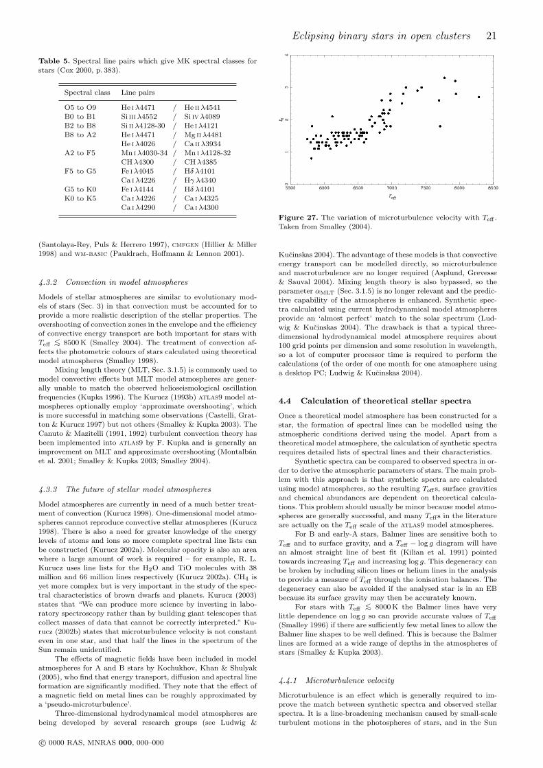
Eclipsing binary stars in open clusters 21
Table 5. Spectral line pairs which give MK spectral classes forstars (Cox 2000, p. 383).
Spectral class Line pairs
O5 to O9 He iλ4471 / He iiλ4541B0 to B1 Si iiiλ4552 / Si ivλ4089B2 to B8 Si iiλ4128-30 / He iλ4121B8 to A2 He iλ4471 / Mg iiλ4481
He iλ4026 / Ca iiλ3934A2 to F5 Mn iλ4030-34 / Mn iλ4128-32
CHλ4300 / CHλ4385F5 to G5 Fe iλ4045 / Hδ λ4101
Ca iλ4226 / Hγ λ4340G5 to K0 Fe iλ4144 / Hδ λ4101K0 to K5 Ca iλ4226 / Ca iλ4325
Ca iλ4290 / Ca iλ4300
(Santolaya-Rey, Puls & Herrero 1997), cmfgen (Hillier & Miller1998) and wm-basic (Pauldrach, Hoffmann & Lennon 2001).
4.3.2 Convection in model atmospheres
Models of stellar atmospheres are similar to evolutionary mod-els of stars (Sec. 3) in that convection must be accounted for toprovide a more realistic description of the stellar properties. Theovershooting of convection zones in the envelope and the efficiencyof convective energy transport are both important for stars withTeff <∼ 8500 K (Smalley 2004). The treatment of convection af-fects the photometric colours of stars calculated using theoreticalmodel atmospheres (Smalley 1998).
Mixing length theory (MLT, Sec. 3.1.5) is commonly used tomodel convective effects but MLT model atmospheres are gener-ally unable to match the observed helioseismological oscillationfrequencies (Kupka 1996). The Kurucz (1993b) atlas9 model at-mospheres optionally employ ‘approximate overshooting’, whichis more successful in matching some observations (Castelli, Grat-ton & Kurucz 1997) but not others (Smalley & Kupka 2003). TheCanuto & Mazitelli (1991, 1992) turbulent convection theory hasbeen implemented into atlas9 by F. Kupka and is generally animprovement on MLT and approximate overshooting (Montalbanet al. 2001; Smalley & Kupka 2003; Smalley 2004).
4.3.3 The future of stellar model atmospheres
Model atmospheres are currently in need of a much better treat-ment of convection (Kurucz 1998). One-dimensional model atmo-spheres cannot reproduce convective stellar atmospheres (Kurucz1998). There is also a need for greater knowledge of the energylevels of atoms and ions so more complete spectral line lists canbe constructed (Kurucz 2002a). Molecular opacity is also an areawhere a large amount of work is required – for example, R. L.Kurucz uses line lists for the H2O and TiO molecules with 38million and 66 million lines respectively (Kurucz 2002a). CH4 isyet more complex but is very important in the study of the spec-tral characteristics of brown dwarfs and planets. Kurucz (2003)states that “We can produce more science by investing in labo-ratory spectroscopy rather than by building giant telescopes thatcollect masses of data that cannot be correctly interpreted.” Ku-rucz (2002b) states that microturbulence velocity is not constanteven in one star, and that half the lines in the spectrum of theSun remain unidentified.
The effects of magnetic fields have been included in modelatmospheres for A and B stars by Kochukhov, Khan & Shulyak(2005), who find that energy transport, diffusion and spectral lineformation are significantly modified. They note that the effect ofa magnetic field on metal lines can be roughly approximated bya ‘pseudo-microturbulence’.
Three-dimensional hydrodynamical model atmospheres arebeing developed by several research groups (see Ludwig &
Figure 27. The variation of microturbulence velocity with Teff .Taken from Smalley (2004).
Kucinskas 2004). The advantage of these models is that convectiveenergy transport can be modelled directly, so microturbulenceand macroturbulence are no longer required (Asplund, Grevesse& Sauval 2004). Mixing length theory is also bypassed, so theparameter αMLT (Sec. 3.1.5) is no longer relevant and the predic-tive capability of the atmospheres is enhanced. Synthetic spec-tra calculated using current hydrodynamical model atmospheresprovide an ‘almost perfect’ match to the solar spectrum (Lud-wig & Kucinskas 2004). The drawback is that a typical three-dimensional hydrodynamical model atmosphere requires about100 grid points per dimension and some resolution in wavelength,so a lot of computer processor time is required to perform thecalculations (of the order of one month for one atmosphere usinga desktop PC; Ludwig & Kucinskas 2004).
4.4 Calculation of theoretical stellar spectra
Once a theoretical model atmosphere has been constructed for astar, the formation of spectral lines can be modelled using theatmospheric conditions derived using the model. Apart from atheoretical model atmosphere, the calculation of synthetic spectrarequires detailed lists of spectral lines and their characteristics.
Synthetic spectra can be compared to observed spectra in or-der to derive the atmospheric parameters of stars. The main prob-lem with this approach is that synthetic spectra are calculatedusing model atmospheres, so the resulting Teffs, surface gravitiesand chemical abundances are dependent on theoretical calcula-tions. This problem should usually be minor because model atmo-spheres are generally successful, and many Teffs in the literatureare actually on the Teff scale of the atlas9 model atmospheres.
For B and early-A stars, Balmer lines are sensitive both toTeff and to surface gravity, and a Teff − log g diagram will havean almost straight line of best fit (Kilian et al. 1991) pointedtowards increasing Teff and increasing log g. This degeneracy canbe broken by including silicon lines or helium lines in the analysisto provide a measure of Teff through the ionisation balances. Thedegeneracy can also be avoided if the analysed star is in an EBbecause its surface gravity may then be accurately known.
For stars with Teff <∼ 8000 K the Balmer lines have verylittle dependence on log g so can provide accurate values of Teff
(Smalley 1996) if there are sufficiently few metal lines to allow theBalmer line shapes to be well defined. This is because the Balmerlines are formed at a wide range of depths in the atmospheres ofstars (Smalley & Kupka 2003).
4.4.1 Microturbulence velocity
Microturbulence is an effect which is generally required to im-prove the match between synthetic spectra and observed stellarspectra. It is a line-broadening mechanism caused by small-scaleturbulent motions in the photospheres of stars, and in the Sun
c© 0000 RAS, MNRAS 000, 000–000
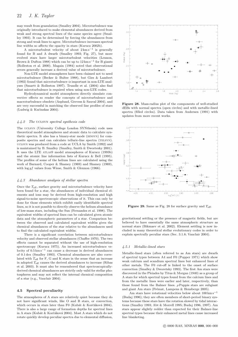
22 J. K. Taylor
may result from granulation (Smalley 2004). Microturbulence wasoriginally introduced to make elemental abundances derived fromweak and strong spectral lines of the same species agree (Smal-ley 1993). It can be determined by forcing the abundances fromstrong and weak lines to agree. Microturbulence increases spectralline widths so affects the opacity in stars (Kurucz 2002b).
A microturbulent velocity of about 2 km s−1 is generallyfound for B and A dwarfs (Smalley 1993; Fig. 27), but moreevolved stars have larger microturbulent velocities (Lennon,Brown & Dufton 1988) which can be up to 12 km s−1 for B giants(Rolleston et al. 2000). Magain (1984) noted that observationalerrors generally increase a derived value of microturbulence.
Non-LTE model atmospheres have been claimed not to needmicroturbulence (Becker & Bulter 1988), but Gies & Lambert(1992) found that microturbulence is important in non-LTE anal-yses (Smartt & Rolleston 1997). Trundle et al. (2004) also findthat microturbulence is required when using non-LTE codes.
Hydrodynamical model atmospheres directly simulate con-vective effects so render the concepts of microturbulence andmacroturbulence obsolete (Asplund, Grevess & Sauval 2004), andare very successful in matching the observed line profiles of stars(Ludwig & Kucinskas 2004).
4.4.2 The uclsyn spectral synthesis code
The uclsyn (University College London SYNthesis) code usestheoretical model atmospheres and atomic data to calculate syn-thetic spectra. It also has a binary-star mode (binsyn) for com-posite spectra and can calculate telluric-line spectra (telsyn).uclsyn was produced from a code at UCLA by Smith (1992) andis maintained by B. Smalley (Smalley, Smith & Dwortesky 2001).It uses the LTE atlas9 model atmospheres of Kurucz (1993b)and the atomic line information lists of Kurucz & Bell (1995).The profiles of some of the helium lines are calculated using thework of Barnard, Cooper & Shamey (1969) and Shamey (1969),with log gf values from Wiese, Smith & Glennon (1966).
4.4.3 Abundance analysis of stellar spectra
Once the Teff , surface gravity and microturbulence velocity havebeen found for a star, the abundances of individual chemical el-ements and ions may be derived from high-resolution and highsignal-to-noise spectroscopic observations of it. This can only bedone for those elements which exhibit easily identifiable spectrallines, so it is not possible to directly observe the helium abundanceof low-mass stars, including the Sun (Fernandes et al. 1998). Theequivalent widths of spectral lines can be calculated given atomicdata and the atmospheric parameters of a star. Comparison be-tween the observed and calculated equivalent widths gives thechemical abundances of the star relative to the abundances usedto find the calculated equivalent widths.
There is a significant correlation between microturbulencevelocity and observed stellar abundances (Chaffee 1970). The twoeffects cannot be separated without the use of high-resolutionspectroscopy (Kurucz 1975). An increased microturbulence ve-locity of 0.5 km s−1 can cause a decrease in derived abundancesof 0.1 dex (Smalley 1993). Chemical abundances are also corre-lated with Teff for F, G and K stars in the sense that an increasein adopted Teff causes the derived abundances to increase (Ribaset al. 2003). It must also be remembered that spectroscopically-derived chemical abundances are strictly only valid for stellar pho-tospheres and may not reflect the internal chemical compositionof a star (e.g., Vauclair 2004).
4.5 Spectral peculiarity
The atmospheres of A stars are relatively quiet because they donot have significant winds, like O and B stars, or convection,which occurs in stars later than F0 (Kubat & Korcakova 2004).There is also a large range of formation depths for spectral linesin A stars (Kubat & Korcakova 2004). Most A stars which do notrotate quickly develop peculiar spectra due to elemental diffusion,
Figure 28. Mass-radius plot of the components of well-studieddEBs with normal spectra (open circles) and with metallic-linedspectra (filled circles). Data taken from Andersen (1991) withupdates from more recent works.
Figure 29. Same as Fig. 28 for surface gravity and Teff .
gravitational settling or the presence of magnetic fields, but arebelieved to have essentially the same atmospheric structure asnormal stars (Bikmaev et al. 2002). Element settling is now in-cluded in many theoretical stellar evolutionary codes in order toexplain spectrally peculiar stars (Sec. 3.1.8; Vauclair 2004).
4.5.1 Metallic-lined stars
Metallic-lined stars (often referred to as Am stars) are dwarfsof spectral types between A4 and F0 (Popper 1971) which showweak calcium and scandium spectral lines but enhanced lines ofother metals. The F0 cut-off is linked to the onset of surfaceconvection (Smalley & Dworetsky 1993). The first Am stars werediscovered in the Pleiades by Titus & Morgan (1940) as a group ofA stars for which spectral types found from the calcium lines andfrom the metallic lines were earlier and later, respectively, thanthose found from the Balmer lines. ρPuppis stars are subgiantand giant Am stars (Fremat, Lampens & Hensberge 2005).
Am stars have rotational velocities below about 100 km s−1
(Budaj 1996); they are often members of short-period binary sys-tems because these stars have the rotation slowed by tidal interac-tions (Smalley 1993; Abt & Morrell 1995; Budaj 1996, 1997). Amstars appear slightly redder than expected for their Balmer-linespectral types because their enhanced metal lines cause increasedline blanketing.
c© 0000 RAS, MNRAS 000, 000–000

Eclipsing binary stars in open clusters 23
Figure 30. Same as Fig. 28 for orbital period and mass.
Figure 31. Same as Fig. 28 for orbital period and radius.
Am stars have often been found to be slightly evolved (e.g.,Kitamura & Kondo 1978) but Dworetsky & Moon (1986) foundthat Am stars in clusters had surface gravities which were negli-gibly different to those of normal A stars. The Am phenomenonends at log g ≈ 3.05 due to the onset of convection (Richer,Michaud & Turcotte 2000).
The metallic-lined phenomenon in stars arises because diffu-sion and gravitational settling cause metallic ions and atoms tomigrate towards the stellar surface. The phenomenon can there-fore be likened to a ‘skin disease’ (J. Andersen, private comunica-tion) in which the surface chemical composition does not reflectthe interior chemical composition of the star. Several well-studieddEBs show metallic-lined spectral characteristics, so their prop-erties can be used to shed light on the Am phenomenon. Figs. 28,29, 30 and 31 compare the characteristics of metallic-lined dEBcomponents to those which exhibit normal spectra. It can be seenthat there is no obvious region in parameter space where all starsare Am, which is consistent with the phenomenon being a surfaceeffect which depends partially on physical properties which havenot been considered here.
4.5.2 Other chemically peculiar stars
Three categories of chemically peculiar (CP) A stars have beenintroduced. CP1 stars are metallic lined stars (see above). CP2stars are Ap (A-type peculiar) stars. CP3 stars are also termedHgMn stars (North, Studer & Kunzli 1997).
Ap stars have variable spectral line profiles and also ex-
hibit photometric variability. They are slow rotators so are ableto exhibit strong magnetic fields, creating starspots which causethe spectral and photometric variability. The magnetic fields alsocause extreme abundance anomalies in which the surface abun-dances of some elements are a thousand times different from nor-mal stars (Abt & Morrell 1995), affecting their spectral energydistributions (Napiwotzki, Schonberger & Wenske 1993).
HgMn stars have Teffs between 11 000 and 15 000 K (spec-tral types B6 to B9) and display abnormally strong mercury andmanganese lines (Wolff 1983, p. 144). These enhancements canbe up to 6 dex for mercury and 3 dex for manganese (Castelli &Hubrig 2004). They are not magnetic stars and their abundanceanomalies are thought to be due to elemental diffusion.
λBootis stars are A-type dwarfs which show normal abun-dances of C, N, O and S, but abnormally weak spectral lines of allother metallic elements (Turcotte 2002). They are spectroscopi-cally similar to Population II stars but have the kinematics ofPopulation I stars, including no dependence of the phenomenonon rotational velocity. They may occur due to the accretion of gaswhich has been depleted by the formation of dust grains (Abt &Morrell 1995). Most λBoo stars are photometrically variable dueto pulsations of the δ Scuti type (Turcotte 2002). Diffusion modelscan simulate λBoo stars, but with difficulty (Turcotte 2002).
5 MULTIPLE STARS
The processes by which stars form naturally also create systemswhich contain two or more stars. Data on stellar multiplicity canbe used to constrain the theories of the formation of star clus-ters, single stars, and of other celestial objects such as planets.The evolution of stars in multiple systems can be very differentto the evolution of single stars. Close binary systems are the soleprogenitors of many exotic objects, so their study and characteri-sation can be very rewarding. The study of binary systems can beregarded as a window through which we can study single stars.
Reasons for studying the multiplicity of stars and the char-acteristics of multiple stars include:–
• constraining star formation theory by statistical study of thedistribution of orbital elements (e.g., Mazeh et al. 1992)
• characterisation of large stellar populations and the lightthey produce (which contains a significant contribution from ob-jects which are only formed by interaction between stars in abinary system)
• finding the age of large stellar systems from comparison ofthe eccentricities of binary systems with tidal evolution theories(section 7.1.5)
• investigating the physics of the evolution of close binaries
• calibrating the M − L relation (Duquennoy & Mayor 1991)
• finding high-mass stellar remnants (Duquennoy & Mayor1991)
• studying how our Galaxy formed (Duquennoy & Mayor 1991)
• multiple stars play an important role in the evolution of grav-itationally bound stellar systems (Mermilliod et al. 1992)
5.1 Dynamical characteristics of multiple stars
From the radial velocity (RV) study of Duquennoy & Mayor(Duquennoy & Mayor 1991; Duquennoy, Mayor & Halbwachs1991), the fraction of nearby F, G and K-type dwarfs which haveone or more companion star is 0.43 and each star has on average0.50 companions. The completeness of this study will drop to-wards low mass ratios as lower-mass secondary components willhave a progressively smaller effect on the radial velocities of theprimary stars. The orbital elements were derived for 37 binary sys-tems and studied statistically. The orbital period distribution wasfound to approximate a Gaussian with a peak at about 180 years,and the median orbital eccentricity was found to be 0.31. Thislast finding is relevant only for systems with periods greater thanabout eleven days, which have not been significantly affected bytidal effects. The binary fraction of evolved stars is much lower
c© 0000 RAS, MNRAS 000, 000–000
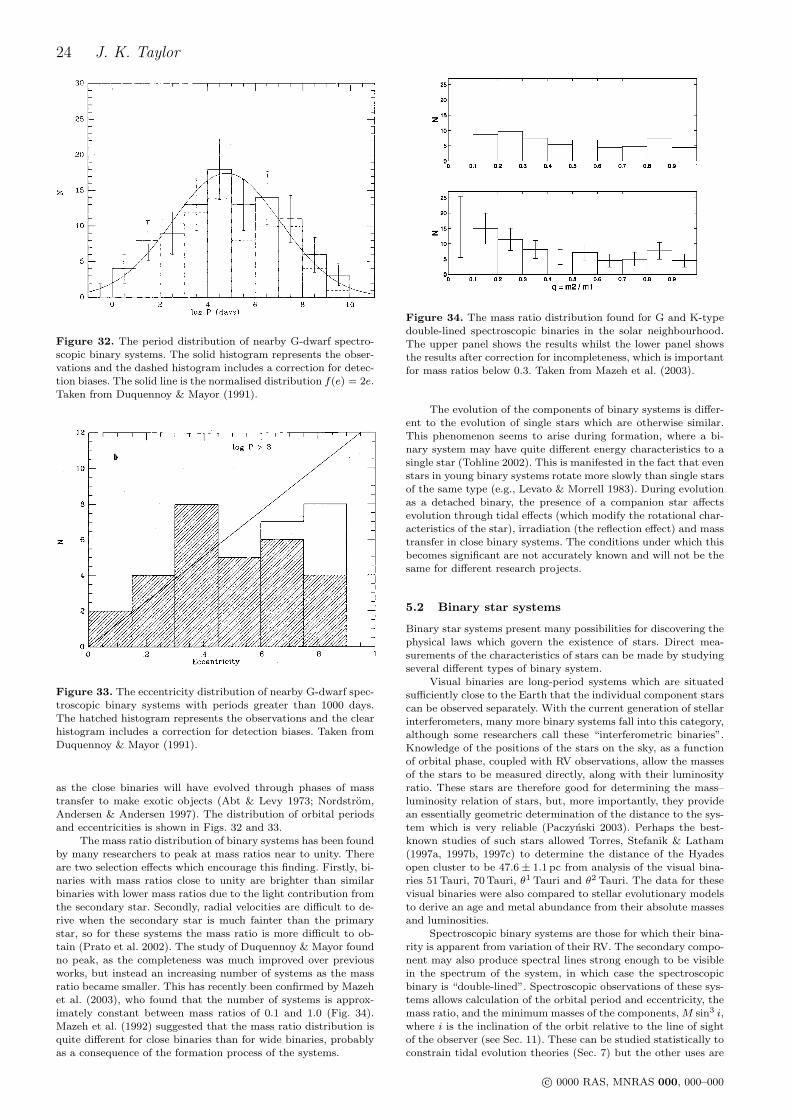
24 J. K. Taylor
Figure 32. The period distribution of nearby G-dwarf spectro-scopic binary systems. The solid histogram represents the obser-vations and the dashed histogram includes a correction for detec-tion biases. The solid line is the normalised distribution f(e) = 2e.Taken from Duquennoy & Mayor (1991).
Figure 33. The eccentricity distribution of nearby G-dwarf spec-troscopic binary systems with periods greater than 1000 days.The hatched histogram represents the observations and the clearhistogram includes a correction for detection biases. Taken fromDuquennoy & Mayor (1991).
as the close binaries will have evolved through phases of masstransfer to make exotic objects (Abt & Levy 1973; Nordstrom,Andersen & Andersen 1997). The distribution of orbital periodsand eccentricities is shown in Figs. 32 and 33.
The mass ratio distribution of binary systems has been foundby many researchers to peak at mass ratios near to unity. Thereare two selection effects which encourage this finding. Firstly, bi-naries with mass ratios close to unity are brighter than similarbinaries with lower mass ratios due to the light contribution fromthe secondary star. Secondly, radial velocities are difficult to de-rive when the secondary star is much fainter than the primarystar, so for these systems the mass ratio is more difficult to ob-tain (Prato et al. 2002). The study of Duquennoy & Mayor foundno peak, as the completeness was much improved over previousworks, but instead an increasing number of systems as the massratio became smaller. This has recently been confirmed by Mazehet al. (2003), who found that the number of systems is approx-imately constant between mass ratios of 0.1 and 1.0 (Fig. 34).Mazeh et al. (1992) suggested that the mass ratio distribution isquite different for close binaries than for wide binaries, probablyas a consequence of the formation process of the systems.
Figure 34. The mass ratio distribution found for G and K-typedouble-lined spectroscopic binaries in the solar neighbourhood.The upper panel shows the results whilst the lower panel showsthe results after correction for incompleteness, which is importantfor mass ratios below 0.3. Taken from Mazeh et al. (2003).
The evolution of the components of binary systems is differ-ent to the evolution of single stars which are otherwise similar.This phenomenon seems to arise during formation, where a bi-nary system may have quite different energy characteristics to asingle star (Tohline 2002). This is manifested in the fact that evenstars in young binary systems rotate more slowly than single starsof the same type (e.g., Levato & Morrell 1983). During evolutionas a detached binary, the presence of a companion star affectsevolution through tidal effects (which modify the rotational char-acteristics of the star), irradiation (the reflection effect) and masstransfer in close binary systems. The conditions under which thisbecomes significant are not accurately known and will not be thesame for different research projects.
5.2 Binary star systems
Binary star systems present many possibilities for discovering thephysical laws which govern the existence of stars. Direct mea-surements of the characteristics of stars can be made by studyingseveral different types of binary system.
Visual binaries are long-period systems which are situatedsufficiently close to the Earth that the individual component starscan be observed separately. With the current generation of stellarinterferometers, many more binary systems fall into this category,although some researchers call these “interferometric binaries”.Knowledge of the positions of the stars on the sky, as a functionof orbital phase, coupled with RV observations, allow the massesof the stars to be measured directly, along with their luminosityratio. These stars are therefore good for determining the mass–luminosity relation of stars, but, more importantly, they providean essentially geometric determination of the distance to the sys-tem which is very reliable (Paczynski 2003). Perhaps the best-known studies of such stars allowed Torres, Stefanik & Latham(1997a, 1997b, 1997c) to determine the distance of the Hyadesopen cluster to be 47.6± 1.1 pc from analysis of the visual bina-ries 51 Tauri, 70 Tauri, θ1 Tauri and θ2 Tauri. The data for thesevisual binaries were also compared to stellar evolutionary modelsto derive an age and metal abundance from their absolute massesand luminosities.
Spectroscopic binary systems are those for which their bina-rity is apparent from variation of their RV. The secondary compo-nent may also produce spectral lines strong enough to be visiblein the spectrum of the system, in which case the spectroscopicbinary is “double-lined”. Spectroscopic observations of these sys-tems allows calculation of the orbital period and eccentricity, themass ratio, and the minimum masses of the components, M sin3 i,where i is the inclination of the orbit relative to the line of sightof the observer (see Sec. 11). These can be studied statistically toconstrain tidal evolution theories (Sec. 7) but the other uses are
c© 0000 RAS, MNRAS 000, 000–000
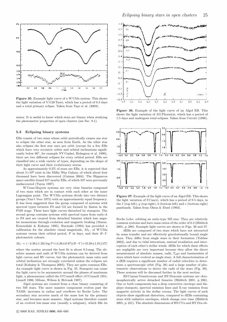
Eclipsing binary stars in open clusters 25
Figure 35. Example light curve of a W UMa system. This showsthe light variation of V1128 Tauri, which has a period of 0.3 daysand a total primary eclipse. Taken from Tacs et al. (2003).
minor. It is useful to know which stars are binary when studyingthe photometric properties of open clusters (see Sec. 8.1).
5.3 Eclipsing binary systems
EBs consist of two stars whose orbit periodically causes one starto eclipse the other star, as seen from Earth. As the other staralso eclipses the first star once per orbit (except for a few EBswhich have very eccentric orbits and orbital inclinations signifi-cantly below 90, for example NY Cephei, Holmgren et al. 1990),there are two different eclipses for every orbital period. EBs areclassified into a wide variety of types, depending on the shape oftheir light curve and their evolutionary status.
As approximately 0.2% of stars are EBs, it is expected thatabout 5×10⁶ exist in the Milky Way Galaxy, of which about fourthousand have been discovered (Guinan 2004). The Hipparcosspace satellite found 917 nearby EBs, of which 347 were previouslyundiscovered (Turon 1997).
W Ursae Majoris systems are very close binaries composedof two stars which are in contact with each other at the innerLagrangian point. The W UMa systems divide into two distinctgroups (Van’t Veer 1975) with an approximately equal frequency.It has been suggested that the group composed of systems withspectral types between F8 and G2 are formed by fission in thePMS stage. These have light curves disturbed by starspots. Thesecond group contains systems with spectral types from early-Ato F8 and are created from detached binaries which lose angu-lar momentum through evolution and magnetic braking (Mazur,Krzeminski & KaÃluzny 1995). Rucinski (1994) has provided acalibration for the absolute visual magnitude, MV , of W UMasystems versus their orbital period, P in days, and their B−Vphotometric colours:
MV = (−2.38±1.20) logP+(4.26±0.87)(B−V )+(0.28±1.01)(47)
where the scatter around the best fit is about 0.5 mag. The ab-solute masses and radii of W UMa systems can be derived fromlight curves and RV curves, but the photometric mass ratio andorbital inclination are strongly correlated unless the eclipses aretotal (KaÃluzny & Thompson 2003). They are quite common EBs.An example light curve is shown in Fig. 35. Starspots can causethe light curve to be asymmetric around the phases of maximumlight, a phenomenon called the O’Connell effect (O’Connell 1951;Linnell 1986; Milone, Wilson & Hrivnak 1987).
Algol systems are created from a close binary consisting oftwo MS stars. The more massive component evolves past theTAMS, increases in radius and overflows its Roche Lobe. Thesecondary star accretes much of the mass lost by the primarystar, and becomes more massive. Algol systems therefore consistof an evolved low-mass star (usually a subgiant), which fills its
Figure 36. Example of the light curve of an Algol EB. Thisshows the light variation of AG Phoenicis, which has a period of1.5 days and undergoes total eclipses. Taken from Cerruti (1996).
Figure 37. Example of the light curve of an Algol EB. This showsthe light variation of S Cancri, which has a period of 9.5 days, inthe I (top left), y (top right), b (bottom left) and v (bottom right)passbands. Taken from Olson & Etzel (1993).
Roche Lobe, orbiting an early-type MS star. They are relativelycommon systems and have mass ratios of the order of 0.3 (Hilditch2001, p. 288). Example light curves are shown in Figs. 36 and 37.
dEBs are composed of two stars which have not interactedby mass transfer and are effectively gravitationally bound singlestars. They differ from single stars in their formation (Tohline2002), and due to tidal interations, mutual irradiation and inter-ception of each other’s stellar winds. dEBs for which these effectsare negligible are very important because they allow the directmeasurement of absolute masses, radii, Teffs and luminosities ofstars which have evolved as single stars. A full characterisation ofa dEB requires a significant number of radial velocities to deter-mine a spectroscopic orbit (Fig. 38) and a large number of pho-tometric observations to derive the radii of the stars (Fig. 39).These systems will be discussed further in the next section.
RS Canum Venaticorum and BY Draconis systems are chro-mospherically active detached binaries (Hilditch 2001, p. 286).One or both components has a deep convective envelope and dis-plays starspots, spectral emission lines and X-ray emission frommagnetic activity in the stellar corona. The light curves of suchobjects show significant distortion, compared to dEBs containingstars with radiative envelopes, which change over time (Hilditch2001, p. 221). The absolute dimensions of RS CVn and BY Dra ob-
c© 0000 RAS, MNRAS 000, 000–000
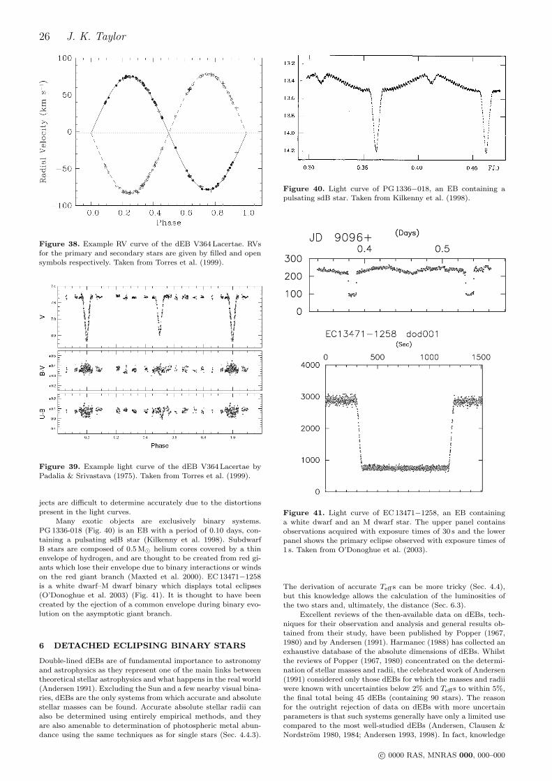
26 J. K. Taylor
Figure 38. Example RV curve of the dEB V364 Lacertae. RVsfor the primary and secondary stars are given by filled and opensymbols respectively. Taken from Torres et al. (1999).
Figure 39. Example light curve of the dEB V364 Lacertae byPadalia & Srivastava (1975). Taken from Torres et al. (1999).
jects are difficult to determine accurately due to the distortionspresent in the light curves.
Many exotic objects are exclusively binary systems.PG 1336-018 (Fig. 40) is an EB with a period of 0.10 days, con-taining a pulsating sdB star (Kilkenny et al. 1998). SubdwarfB stars are composed of 0.5 M¯ helium cores covered by a thinenvelope of hydrogen, and are thought to be created from red gi-ants which lose their envelope due to binary interactions or windson the red giant branch (Maxted et al. 2000). EC 13471−1258is a white dwarf–M dwarf binary which displays total eclipses(O’Donoghue et al. 2003) (Fig. 41). It is thought to have beencreated by the ejection of a common envelope during binary evo-lution on the asymptotic giant branch.
6 DETACHED ECLIPSING BINARY STARS
Double-lined dEBs are of fundamental importance to astronomyand astrophysics as they represent one of the main links betweentheoretical stellar astrophysics and what happens in the real world(Andersen 1991). Excluding the Sun and a few nearby visual bina-ries, dEBs are the only systems from which accurate and absolutestellar masses can be found. Accurate absolute stellar radii canalso be determined using entirely empirical methods, and theyare also amenable to determination of photospheric metal abun-dance using the same techniques as for single stars (Sec. 4.4.3).
Figure 40. Light curve of PG 1336−018, an EB containing apulsating sdB star. Taken from Kilkenny et al. (1998).
Figure 41. Light curve of EC 13471−1258, an EB containinga white dwarf and an M dwarf star. The upper panel containsobservations acquired with exposure times of 30 s and the lowerpanel shows the primary eclipse observed with exposure times of1 s. Taken from O’Donoghue et al. (2003).
The derivation of accurate Teffs can be more tricky (Sec. 4.4),but this knowledge allows the calculation of the luminosities ofthe two stars and, ultimately, the distance (Sec. 6.3).
Excellent reviews of the then-available data on dEBs, tech-niques for their observation and analysis and general results ob-tained from their study, have been published by Popper (1967,1980) and by Andersen (1991). Harmanec (1988) has collected anexhaustive database of the absolute dimensions of dEBs. Whilstthe reviews of Popper (1967, 1980) concentrated on the determi-nation of stellar masses and radii, the celebrated work of Andersen(1991) considered only those dEBs for which the masses and radiiwere known with uncertainties below 2% and Teffs to within 5%,the final total being 45 dEBs (containing 90 stars). The reasonfor the outright rejection of data on dEBs with more uncertainparameters is that such systems generally have only a limited usecompared to the most well-studied dEBs (Andersen, Clausen &Nordstrom 1980, 1984; Andersen 1993, 1998). In fact, knowledge
c© 0000 RAS, MNRAS 000, 000–000

Eclipsing binary stars in open clusters 27
Figure 42. Logarithmic mass-radius diagram containing thecomponents of well-studied dEBs. Uncertainties are shown as er-rorbars and the theoretical ZAMS for a solar composition, takenfrom the Cambridge stellar evolutionary models (Pols et al. 1998),is given by a solid line.
Figure 43. Logarithmic mass-radius diagram containing thecomponents of well-studied dEBs. The primary components ofdEBs are shown using filled circles and the secondary compo-nents by open circles. Dotted lines connect the components ofindividual dEBs. The theoretical ZAMS for a solar composition,taken from the Cambridge stellar evolutionary models (Pols et al.1998), is given by a solid line.
of the dimensions of a dEB to within 5% is no longer in generaluseful (e.g., Andersen 1991, Gimenez 1992).
Whilst there are a good number of well-studied MS dEBsof spectral types between B and G, very few exist outside theseboundaries. Whilst several O star dEBs have been studied (e.g.,V1007 Scorpii, Sana, Rauw & Gosset 2001), these systems ex-hibit complications which makes determination of accurate pa-rameters very difficult. dEBs known to contain K or M dwarfsare very rare as the small sizes of these stars means that fewexhibit deep eclipses (Popper 1993). Starspots can also be prob-lematic when analysing the light curves of such systems (seee.g., Torres & Ribas 2002; Ribas 2003). There is also a short-age of dEB components which are close to the ZAMS (Ander-sen 1991, Gimenez 1992), particularly for high-mass stars, andbeyond the TAMS (with the important exceptions of the giantsystem TZ Fornacis, Andersen et al. 1991, and SZ Centauri, An-dersen 1975c). This is because dEBs which contain an evolvedstar tend to exhibit single-lined spectra as the unevolved star is alot dimmer than the evolved star. Therefore dEBs which containan evolved star but are double-lined must have a mass ratio closeto unity (Andersen 1975c), so are very rare. Recent work has be-gun to focus on dEBs containing substellar objects (e.g., 2MASS
Figure 44. Logarithmic Teff -log g diagram containing the com-ponents of well-studied dEBs. Symbols are as in Fig. 42.
Figure 45. Logarithmic Teff -log g diagram containing the com-ponents of well-studied dEBs. Symbols are as in Fig. 43.
J0516288+260738, which appears to be an eclipsing M dwarf –brown dwarf system, Schuh et al. 2003).
The available data on dEBs with masses and radii accurateto 2%, and Teffs to within 5%, has been collected from Andersen(1991). Results from more recent publications have been added,with an emphasis on the inclusion of interesting dEBs rather thanthose which conform precisely to the above limits on accuracy.These have been plotted in mass-radius diagrams (Figs. 42 and43) with errors (Fig. 42) or with lines connecting different starsin one dEB (Fig. 43). The corresponding Teff -log g diagrams andHR diagrams have also been plotted in Figs. 44, 45, 46 and 47.
There are two main uses of the fundamental astrophysical pa-rameters of dEBs: as calibrators and checks of theoretical models,and as standard candles. The methods of determining the distanceto different types of dEB will be covered in the next section; otheruses of dEBs will be discussed here.
Knowledge of the masses and radii of the components ofdEBs has allowed Ribas et al. (1997) to construct photometriccalibrations which predict the masses and radii of single stars us-ing Stromgren photometric indices (Sec. 12.1.3). This study up-dates the calibration contained in the uvbybeta code of Moon &Dworetsky (Moon 1985a), which was based on finding the abso-lute magnitude and surface brightness of a star in order to predictits radius. Calibrations of surface brightness could be aided bystudy of the dEBs suggested by Kruszewski & Semeniuk (1999).
c© 0000 RAS, MNRAS 000, 000–000
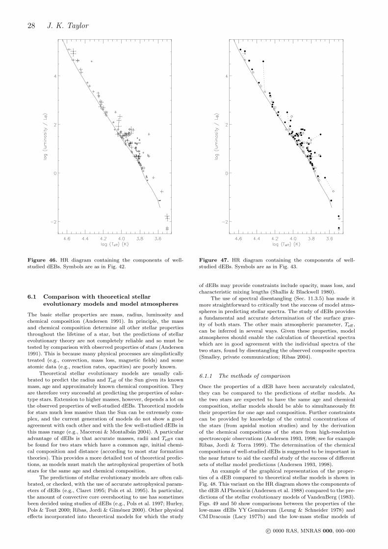
28 J. K. Taylor
Figure 46. HR diagram containing the components of well-studied dEBs. Symbols are as in Fig. 42.
6.1 Comparison with theoretical stellarevolutionary models and model atmospheres
The basic stellar properties are mass, radius, luminosity andchemical composition (Andersen 1991). In principle, the massand chemical composition determine all other stellar propertiesthroughout the lifetime of a star, but the predictions of stellarevolutionary theory are not completely reliable and so must betested by comparison with observed properties of stars (Andersen1991). This is because many physical processes are simplisticallytreated (e.g., convection, mass loss, magnetic fields) and someatomic data (e.g., reaction rates, opacities) are poorly known.
Theoretical stellar evolutionary models are usually cali-brated to predict the radius and Teff of the Sun given its knownmass, age and approximately known chemical composition. Theyare therefore very successful at predicting the properties of solar-type stars. Extension to higher masses, however, depends a lot onthe observed properties of well-studied dEBs. Theoretical modelsfor stars much less massive than the Sun can be extremely com-plex, and the current generation of models do not show a goodagreement with each other and with the few well-studied dEBs inthis mass range (e.g., Maceroni & Montalban 2004). A particularadvantage of dEBs is that accurate masses, radii and Teffs canbe found for two stars which have a common age, initial chemi-cal composition and distance (according to most star formationtheories). This provides a more detailed test of theoretical predic-tions, as models must match the astrophysical properties of bothstars for the same age and chemical composition.
The predictions of stellar evolutionary models are often cali-brated, or checked, with the use of accurate astrophysical param-eters of dEBs (e.g., Claret 1995; Pols et al. 1995). In particular,the amount of convective core overshooting to use has sometimesbeen decided using studies of dEBs (e.g., Pols et al. 1997; Hurley,Pols & Tout 2000; Ribas, Jordi & Gimenez 2000). Other physicaleffects incorporated into theoretical models for which the study
Figure 47. HR diagram containing the components of well-studied dEBs. Symbols are as in Fig. 43.
of dEBs may provide constraints include opacity, mass loss, andcharacteristic mixing lengths (Shallis & Blackwell 1980).
The use of spectral disentangling (Sec. 11.3.5) has made itmore straightforward to critically test the success of model atmo-spheres in predicting stellar spectra. The study of dEBs providesa fundamental and accurate determination of the surface grav-ity of both stars. The other main atmospheric parameter, Teff ,can be inferred in several ways. Given these properties, modelatmospheres should enable the calculation of theoretical spectrawhich are in good agreement with the individual spectra of thetwo stars, found by disentangling the observed composite spectra(Smalley, private communication; Ribas 2004).
6.1.1 The methods of comparison
Once the properties of a dEB have been accurately calculated,they can be compared to the predictions of stellar models. Asthe two stars are expected to have the same age and chemicalcomposition, stellar models should be able to simultaneously fittheir properties for one age and composition. Further constraintscan be provided by knowledge of the central concentrations ofthe stars (from apsidal motion studies) and by the derivationof the chemical compositions of the stars from high-resolutionspectroscopic observations (Andersen 1993, 1998; see for exampleRibas, Jordi & Torra 1999). The determination of the chemicalcompositions of well-studied dEBs is suggested to be important inthe near future to aid the careful study of the success of differentsets of stellar model predictions (Andersen 1993, 1998).
An example of the graphical representation of the proper-ties of a dEB compared to theoretical stellar models is shown inFig. 48. This variant on the HR diagram shows the components ofthe dEB AI Phoenicis (Andersen et al. 1988) compared to the pre-dictions of the stellar evolutionary models of VandenBerg (1983).Figs. 49 and 50 show comparisons between the properties of thelow-mass dEBs YY Geminorum (Leung & Schneider 1978) andCM Draconis (Lacy 1977b) and the low-mass stellar models of
c© 0000 RAS, MNRAS 000, 000–000
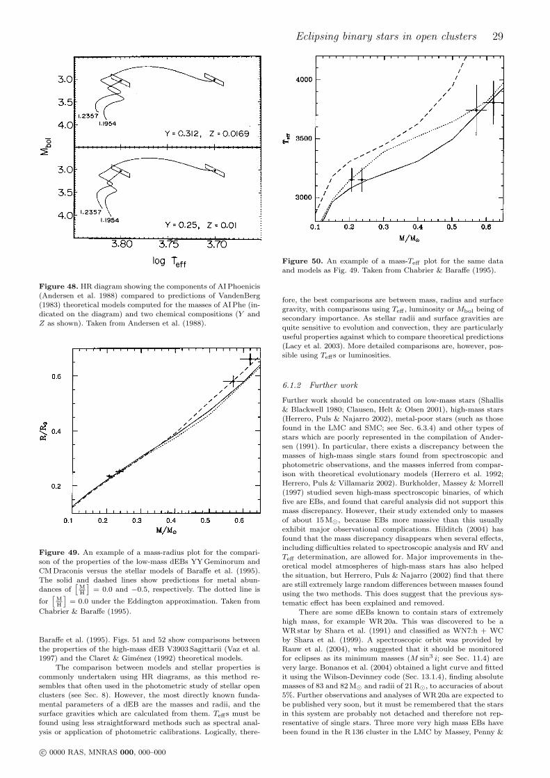
Eclipsing binary stars in open clusters 29
Figure 48. HR diagram showing the components of AI Phoenicis(Andersen et al. 1988) compared to predictions of VandenBerg(1983) theoretical models computed for the masses of AI Phe (in-dicated on the diagram) and two chemical compositions (Y andZ as shown). Taken from Andersen et al. (1988).
Figure 49. An example of a mass-radius plot for the compari-son of the properties of the low-mass dEBs YY Geminorum andCM Draconis versus the stellar models of Baraffe et al. (1995).The solid and dashed lines show predictions for metal abun-dances of
[MH
]= 0.0 and −0.5, respectively. The dotted line is
for[
MH
]= 0.0 under the Eddington approximation. Taken from
Chabrier & Baraffe (1995).
Baraffe et al. (1995). Figs. 51 and 52 show comparisons betweenthe properties of the high-mass dEB V3903 Sagittarii (Vaz et al.1997) and the Claret & Gimenez (1992) theoretical models.
The comparison between models and stellar properties iscommonly undertaken using HR diagrams, as this method re-sembles that often used in the photometric study of stellar openclusters (see Sec. 8). However, the most directly known funda-mental parameters of a dEB are the masses and radii, and thesurface gravities which are calculated from them. Teffs must befound using less straightforward methods such as spectral anal-ysis or application of photometric calibrations. Logically, there-
Figure 50. An example of a mass-Teff plot for the same dataand models as Fig. 49. Taken from Chabrier & Baraffe (1995).
fore, the best comparisons are between mass, radius and surfacegravity, with comparisons using Teff , luminosity or Mbol being ofsecondary importance. As stellar radii and surface gravities arequite sensitive to evolution and convection, they are particularlyuseful properties against which to compare theoretical predictions(Lacy et al. 2003). More detailed comparisons are, however, pos-sible using Teffs or luminosities.
6.1.2 Further work
Further work should be concentrated on low-mass stars (Shallis& Blackwell 1980; Clausen, Helt & Olsen 2001), high-mass stars(Herrero, Puls & Najarro 2002), metal-poor stars (such as thosefound in the LMC and SMC; see Sec. 6.3.4) and other types ofstars which are poorly represented in the compilation of Ander-sen (1991). In particular, there exists a discrepancy between themasses of high-mass single stars found from spectroscopic andphotometric observations, and the masses inferred from compar-ison with theoretical evolutionary models (Herrero et al. 1992;Herrero, Puls & Villamariz 2002). Burkholder, Massey & Morrell(1997) studied seven high-mass spectroscopic binaries, of whichfive are EBs, and found that careful analysis did not support thismass discrepancy. However, their study extended only to massesof about 15 M¯, because EBs more massive than this usuallyexhibit major observational complications. Hilditch (2004) hasfound that the mass discrepancy disappears when several effects,including difficulties related to spectroscopic analysis and RV andTeff determination, are allowed for. Major improvements in the-oretical model atmospheres of high-mass stars has also helpedthe situation, but Herrero, Puls & Najarro (2002) find that thereare still extremely large random differences between masses foundusing the two methods. This does suggest that the previous sys-tematic effect has been explained and removed.
There are some dEBs known to contain stars of extremelyhigh mass, for example WR 20a. This was discovered to be aWR star by Shara et al. (1991) and classified as WN7:h + WCby Shara et al. (1999). A spectroscopic orbit was provided byRauw et al. (2004), who suggested that it should be monitoredfor eclipses as its minimum masses (M sin3 i; see Sec. 11.4) arevery large. Bonanos et al. (2004) obtained a light curve and fittedit using the Wilson-Devinney code (Sec. 13.1.4), finding absolutemasses of 83 and 82 M¯ and radii of 21 R¯, to accuracies of about5%. Further observations and analyses of WR 20a are expected tobe published very soon, but it must be remembered that the starsin this system are probably not detached and therefore not rep-resentative of single stars. Three more very high mass EBs havebeen found in the R 136 cluster in the LMC by Massey, Penny &
c© 0000 RAS, MNRAS 000, 000–000
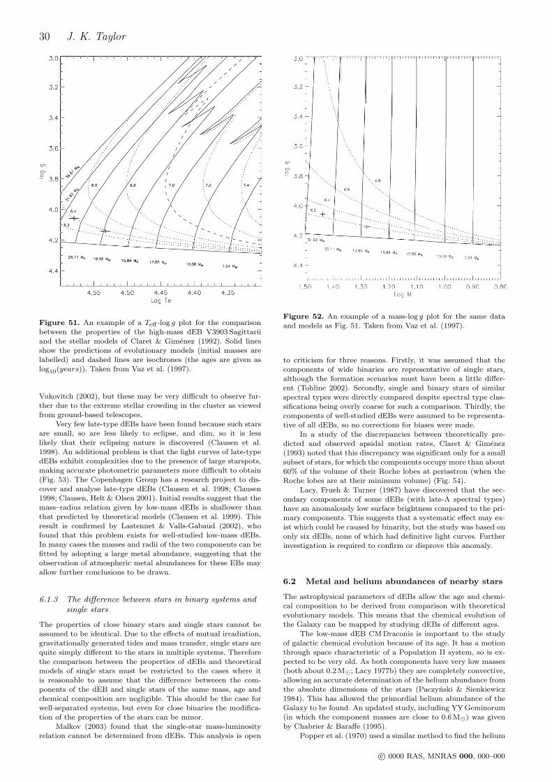
30 J. K. Taylor
Figure 51. An example of a Teff -log g plot for the comparisonbetween the properties of the high-mass dEB V3903 Sagittariiand the stellar models of Claret & Gimenez (1992). Solid linesshow the predictions of evolutionary models (initial masses arelabelled) and dashed lines are isochrones (the ages are given aslog10(years)). Taken from Vaz et al. (1997).
Vukovitch (2002), but these may be very difficult to observe fur-ther due to the extreme stellar crowding in the cluster as viewedfrom ground-based telescopes.
Very few late-type dEBs have been found because such starsare small, so are less likely to eclipse, and dim, so it is lesslikely that their eclipsing nature is discovered (Clausen et al.1998). An additional problem is that the light curves of late-typedEBs exhibit complexities due to the presence of large starspots,making accurate photometric parameters more difficult to obtain(Fig. 53). The Copenhagen Group has a research project to dis-cover and analyse late-type dEBs (Clausen et al. 1998; Clausen1998; Clausen, Helt & Olsen 2001). Initial results suggest that themass–radius relation given by low-mass dEBs is shallower thanthat predicted by theoretical models (Clausen et al. 1999). Thisresult is confirmed by Lastennet & Valls-Gabaud (2002), whofound that this problem exists for well-studied low-mass dEBs.In many cases the masses and radii of the two components can befitted by adopting a large metal abundance, suggesting that theobservation of atmospheric metal abundances for these EBs mayallow further conclusions to be drawn.
6.1.3 The difference between stars in binary systems andsingle stars
The properties of close binary stars and single stars cannot beassumed to be identical. Due to the effects of mutual irradiation,gravitationally generated tides and mass transfer, single stars arequite simply different to the stars in multiple systems. Thereforethe comparison between the properties of dEBs and theoreticalmodels of single stars must be restricted to the cases where itis reasonable to assume that the difference betweeen the com-ponents of the dEB and single stars of the same mass, age andchemical composition are negligible. This should be the case forwell-separated systems, but even for close binaries the modifica-tion of the properties of the stars can be minor.
Malkov (2003) found that the single-star mass-luminosityrelation cannot be determined from dEBs. This analysis is open
Figure 52. An example of a mass-log g plot for the same dataand models as Fig. 51. Taken from Vaz et al. (1997).
to criticism for three reasons. Firstly, it was assumed that thecomponents of wide binaries are representative of single stars,although the formation scenarios must have been a little differ-ent (Tohline 2002). Secondly, single and binary stars of similarspectral types were directly compared despite spectral type clas-sifications being overly coarse for such a comparison. Thirdly, thecomponents of well-studied dEBs were assumed to be representa-tive of all dEBs, so no corrections for biases were made.
In a study of the discrepancies between theoretically pre-dicted and observed apsidal motion rates, Claret & Gimenez(1993) noted that this discrepancy was significant only for a smallsubset of stars, for which the components occupy more than about60% of the volume of their Roche lobes at periastron (when theRoche lobes are at their minimum volume) (Fig. 54).
Lacy, Frueh & Turner (1987) have discovered that the sec-ondary components of some dEBs (with late-A spectral types)have an anomalously low surface brightness compared to the pri-mary components. This suggests that a systematic effect may ex-ist which could be caused by binarity, but the study was based ononly six dEBs, none of which had definitive light curves. Furtherinvestigation is required to confirm or disprove this anomaly.
6.2 Metal and helium abundances of nearby stars
The astrophysical parameters of dEBs allow the age and chemi-cal composition to be derived from comparison with theoreticalevolutionary models. This means that the chemical evolution ofthe Galaxy can be mapped by studying dEBs of different ages.
The low-mass dEB CM Draconis is important to the studyof galactic chemical evolution because of its age. It has a motionthrough space characteristic of a Population II system, so is ex-pected to be very old. As both components have very low masses(both about 0.2 M¯; Lacy 1977b) they are completely convective,allowing an accurate determination of the helium abundance fromthe absolute dimensions of the stars (Paczynski & Sienkiewicz1984). This has allowed the primordial helium abundance of theGalaxy to be found. An updated study, including YY Geminorum(in which the component masses are close to 0.6 M¯) was givenby Chabrier & Baraffe (1995).
Popper et al. (1970) used a similar method to find the helium
c© 0000 RAS, MNRAS 000, 000–000
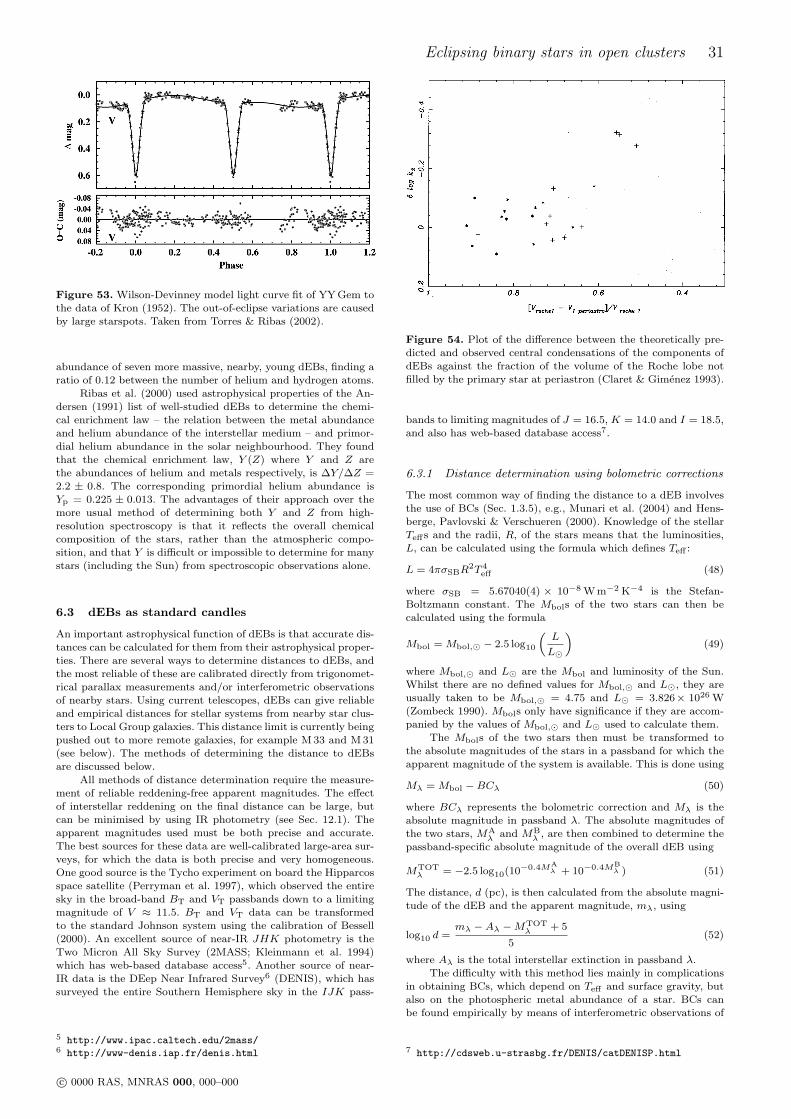
Eclipsing binary stars in open clusters 31
Figure 53. Wilson-Devinney model light curve fit of YY Gem tothe data of Kron (1952). The out-of-eclipse variations are causedby large starspots. Taken from Torres & Ribas (2002).
abundance of seven more massive, nearby, young dEBs, finding aratio of 0.12 between the number of helium and hydrogen atoms.
Ribas et al. (2000) used astrophysical properties of the An-dersen (1991) list of well-studied dEBs to determine the chemi-cal enrichment law – the relation between the metal abundanceand helium abundance of the interstellar medium – and primor-dial helium abundance in the solar neighbourhood. They foundthat the chemical enrichment law, Y (Z) where Y and Z arethe abundances of helium and metals respectively, is ∆Y/∆Z =2.2 ± 0.8. The corresponding primordial helium abundance isYp = 0.225 ± 0.013. The advantages of their approach over themore usual method of determining both Y and Z from high-resolution spectroscopy is that it reflects the overall chemicalcomposition of the stars, rather than the atmospheric compo-sition, and that Y is difficult or impossible to determine for manystars (including the Sun) from spectroscopic observations alone.
6.3 dEBs as standard candles
An important astrophysical function of dEBs is that accurate dis-tances can be calculated for them from their astrophysical proper-ties. There are several ways to determine distances to dEBs, andthe most reliable of these are calibrated directly from trigonomet-rical parallax measurements and/or interferometric observationsof nearby stars. Using current telescopes, dEBs can give reliableand empirical distances for stellar systems from nearby star clus-ters to Local Group galaxies. This distance limit is currently beingpushed out to more remote galaxies, for example M 33 and M 31(see below). The methods of determining the distance to dEBsare discussed below.
All methods of distance determination require the measure-ment of reliable reddening-free apparent magnitudes. The effectof interstellar reddening on the final distance can be large, butcan be minimised by using IR photometry (see Sec. 12.1). Theapparent magnitudes used must be both precise and accurate.The best sources for these data are well-calibrated large-area sur-veys, for which the data is both precise and very homogeneous.One good source is the Tycho experiment on board the Hipparcosspace satellite (Perryman et al. 1997), which observed the entiresky in the broad-band BT and VT passbands down to a limitingmagnitude of V ≈ 11.5. BT and VT data can be transformedto the standard Johnson system using the calibration of Bessell(2000). An excellent source of near-IR JHK photometry is theTwo Micron All Sky Survey (2MASS; Kleinmann et al. 1994)which has web-based database access5. Another source of near-IR data is the DEep Near Infrared Survey6 (DENIS), which hassurveyed the entire Southern Hemisphere sky in the IJK pass-
5 http://www.ipac.caltech.edu/2mass/6 http://www-denis.iap.fr/denis.html
Figure 54. Plot of the difference between the theoretically pre-dicted and observed central condensations of the components ofdEBs against the fraction of the volume of the Roche lobe notfilled by the primary star at periastron (Claret & Gimenez 1993).
bands to limiting magnitudes of J = 16.5, K = 14.0 and I = 18.5,and also has web-based database access7.
6.3.1 Distance determination using bolometric corrections
The most common way of finding the distance to a dEB involvesthe use of BCs (Sec. 1.3.5), e.g., Munari et al. (2004) and Hens-berge, Pavlovski & Verschueren (2000). Knowledge of the stellarTeffs and the radii, R, of the stars means that the luminosities,L, can be calculated using the formula which defines Teff :
L = 4πσSBR2T 4
eff (48)
where σSB = 5.67040(4) × 10−8 W m−2 K−4 is the Stefan-Boltzmann constant. The Mbols of the two stars can then becalculated using the formula
Mbol = Mbol,¯ − 2.5 log10
(L
L¯
)(49)
where Mbol,¯ and L¯ are the Mbol and luminosity of the Sun.Whilst there are no defined values for Mbol,¯ and L¯, they areusually taken to be Mbol,¯ = 4.75 and L¯ = 3.826× 1026 W(Zombeck 1990). Mbols only have significance if they are accom-panied by the values of Mbol,¯ and L¯ used to calculate them.
The Mbols of the two stars then must be transformed tothe absolute magnitudes of the stars in a passband for which theapparent magnitude of the system is available. This is done using
Mλ = Mbol −BCλ (50)
where BCλ represents the bolometric correction and Mλ is theabsolute magnitude in passband λ. The absolute magnitudes ofthe two stars, MA
λ and MBλ , are then combined to determine the
passband-specific absolute magnitude of the overall dEB using
MTOTλ = −2.5 log10(10−0.4MA
λ + 10−0.4MBλ ) (51)
The distance, d (pc), is then calculated from the absolute magni-tude of the dEB and the apparent magnitude, mλ, using
log10 d =mλ −Aλ −MTOT
λ + 5
5(52)
where Aλ is the total interstellar extinction in passband λ.
The difficulty with this method lies mainly in complicationsin obtaining BCs, which depend on Teff and surface gravity, butalso on the photospheric metal abundance of a star. BCs canbe found empirically by means of interferometric observations of
7 http://cdsweb.u-strasbg.fr/DENIS/catDENISP.html
c© 0000 RAS, MNRAS 000, 000–000
32 J. K. Taylor
nearby stars with accurate trigonometrical parallaxes, or by UV,optical and IR spectrophotometry (e.g., Code et al. 1976; Ha-bets & Heintze 1981; Malagnini et al. 1986; Flower 1996), butthe resulting BCs are subject to observational uncertainties andare often only relevant to stars with an approximately solar metalabundance. Alternatively, theoretical BCs can be calculated usingmodel atmospheres (e.g., Bessell, Castelli & Plez 1998; Girardi etal. 2002). The advantage of this approach is that observationaluncertainties are entirely avoided and BCs can be calculated fora wide range of chemical compositions. However, using theoreti-cal BCs does introduce a dependence on stellar models into theresulting distance, so theoretical BCs should be avoided, if pos-sible, or carefully compared to empirical BCs. Further discussionon BCs can be found in Sec. 1.3.5.
BCs are quite uncertain for hot stars because these starsemit a large fraction of their radiation in the UV, where it isstrongly absorbed by the interstellar medium. Therefore this dis-tance determination method is not a good one for OB stars (Har-ries, Hilditch & Howarth 2003).
The zeropoint of the BC scale is set by the assumption ofcertain values for Mbol,¯, L¯ and BC¯. This means that BCsare only relevant if they are applied to Mbols which have beencalculated using the same values for Mbol,¯ and L¯. In this case,the zeropoints coincide and a meaningful answer is found (Bessell,Castelli & Plez 1998). The use of different zeropoints means thatthe final answer is meaningless (e.g., Munari et al. 2004).
The measurement of distances using BCs requires that theTeffs of the stars must be derived consistently with the funda-mental definition of Teff ; so the Teff scale has known small ornegligible systematic errors. Determination of Teff is discussed inSec. 4.4. This constraint is important as it can be very difficultto quantify systematic errors in Teff scales.
A good example of this distance determination technique, us-ing empirical BCs, is for V578 Monocerotis (Hensberge, Pavlovski& Verschueren 2000). This method has also been discussed byClausen (2004); he finds that the main uncertainty comes fromthe calibrations for empirical BCs.
6.3.2 Distances using surface brightness calibrations
In this method, the angular diameter of each component of anEB is estimated using the apparent magnitude of the star andcalibrations between surface brightness and one or several photo-metric properties. The linear radius of each star is known froma light and RV curve analysis, and comparison between this andthe angular diameter of each star gives its distance (Lacy 1977a).One distance estimate is obtained for each star – the two esti-mates should be in agreement – and these can be combined usingweighted means, although careful consideration of the uncertain-ties and the correlations in the results is necessary.
Surface brightness relations have been discussed in Sec. 1.3.6and generally comprise a calibration between some measure ofthe visual surface brightness of a star (in magnitudes) and anobserved photometric index. Lacy (1977a) adopted the Barnes-Evans relation (Barnes & Evans 1976) between FV and the V−Rindex. FV is defined to be
FV = log Teff + 0.1BC = 4.2207− 0.1V0 − 0.5 log φ (53)
where BC is the bolometric correction, V0 is the dereddened ap-parent visual magnitude and φ is the angular diameter in milliarc-seconds. FV is given as linear functions of (V−R)0 for differenttypes of star. The distance (in parsecs) is then found from
d = 9.3048R
φ(54)
where R is the stellar radius (in solar units). Individual V0 mag-nitudes and (V−R)0 indices must be determined for the two starsin the dEB from the apparent V magnitude, light curves in theV and R passbands, and a known visual absorption, AV .
Lacy (1977a) applied the above method to nine dEBs forwhich accurate parallaxes were available, finding that distancemoduli derived using the Barnes-Evans relation had accuracies of
about 0.2 mag and were in agreement with distances found us-ing the parallax measurements. Lacy (1978) applied the methodto CW Cephei, V453 Cygni and AG Persei, all members of nearbyopen clusters or associations, and found that the distances derivedwere in agreement with, although slightly larger than, distancesfound from main-sequence fitting analyses of the stellar associa-tions of which the dEBs were members. Lacy (1979) then appliedthe tested method to 48 dEBs, finding that their absolute mag-nitudes were in good agreement with theoretical predictions.
Semeniuk (2000) has compared the method of Lacy (1977a)to other distance determination methods and found that it is ro-bust as long as it is used on well-behaved dEBs; single-star surfacebrightness relations are not applicable to interacting binaries.
6.3.3 Distance determination by modelling stellar spectralenergy distributions
This distance determination method was introduced by Fitz-patrick & Massa (1999) and has been used to find the distance tofour EBs in the LMC: HV 2274 (Guinan et al. 1998; Ribas et al.2000), HV 982 (Fitzpatrick et al. 2002), EROS 1044 (Ribas et al.2002) and HV 5936 (Fitzpatrick et al. 2003).
The principle of this method is to determine the physicalparameters of an early-type EB by fitting Kurucz atlas9 theo-retical model atmospheres to UV and optical spectrophotometry.The observed spectral energy distribution of an EB at the Earthis a function of wavelength, λ;
fλ,⊕ =R 2
A FA,λ +R 2B FB,λ
d2× 10−0.4Aλ (55)
where Fi,λ (i = A,B) are the emergent fluxes at the surfaces ofthe two stars, Ri are the radii of the stars and Aλ is the totalextinction along the line of sight of the EB. Therefore
fλ,⊕ =
(RA
d
)2[FA,λ +
(RB
RA
)2
FB,λ
]10−0.4EB−V
[k(λ−V )+RV
](56)
where EB−V is the reddening, k(λ − V ) ≡ E(λ−V )EB−V
is the ex-
tinction curve and RV = AVEB−V
is the ratio of selective to total
absorption in the V passband.
Synthetic spectra from the model atmospheres are fitted tothe observed fλ,⊕, using nonlinear least squares algorithms, to
derive values for(
RAd
)2, Fi,λ, EB−V and k(λ−V ). The distance
estimate is found directly from(
RAd
)2and the radius of the pri-
mary star. The atlas9 model atmospheres, which represent thesurface fluxes, Fi,λ, depend on Teff , surface gravity, metallicityand microturbulence velocity. Fitzpatrick & Massa (1999) foundthat the atlas9 predictions provide a match to observations at alevel consistent with current uncertainties in spectrophotometricobservations. In addition, it can be assumed that the metallicityand microturbulence velocity of both components is the same.The ratio of the Teffs of the stars is also known from light curveanalysis. Thus there are only five parameters needed to specifyatlas9 model spectral energy distributions of the two stars.
6.3.4 Recent results for the distance to EBs
The main research area currently involving the observation andanalysis of EBs is to use their properties as standard candlesto determine the distances to Local Group galaxies. The first de-tailed photometric study of a dEB outside the Milky Way Galaxywas that of Jensen, Clausen & Gimenez (1988), who provided thefirst CCD light curves of dEBs in the Magellanic Clouds.
The Copenhagen (Denmark) group has continued to studydEBs in the Magellanic Clouds (see Clausen 2000 and Clausenet al. 2003) in order to test the predictions of theoretical stel-lar evolutionary models in the low-metallicity environment of theMagellanic Clouds. The Villanova (USA) group (Guinan et al.1998; Ribas et al. 2000, 2002; Fitzpatrick et al. 2002, 2003) arecontinuing their efforts (detailed above). The Mount John (NewZealand) group are also running an observing program to obtain
c© 0000 RAS, MNRAS 000, 000–000
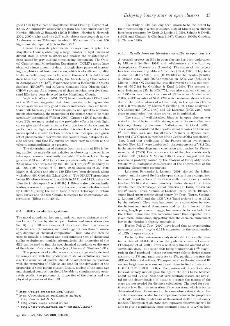
Eclipsing binary stars in open clusters 33
good CCD light curves of Magellanic Cloud EBs (e.g., Bayne et al.2004). An impressive observing program has been undertaken byHarries, Hilditch & Howarth (2003; Hilditch, Harries & Howarth2004, 2005), who used the 2dF multi-object spectrograph at theAnglo-Australian Telescope to obtain RV curves of about 100high-mass short-period EBs in the SMC.
Recent large-scale photometric surveys have targeted theMagellanic Clouds, obtaining a large number of light curves ofdistant stars in order to detect and analyse the brightening ef-fects caused by gravitational microlensing phenomena. The Opti-cal Gravitational Microlensing Experiment (OGLE8) group haveobtained a huge amount of data, through three phases of increas-ingly sophisticated instrumentation, which is of sufficient qualityto derive preliminary results for several thousand EBs. Additionaldata have also been obtained by the Microlensing Observationsin Astrophysics (MOA9), Experience pour la Recherche d’ObjetsSombres (EROS10) and MAssive Compact Halo Objects (MA-CHO11) groups. As a byproduct of these searches, over five thou-sand EBs have been detected in the Magellanic Clouds.
Wyithe & Wilson (2001, 2002) have investigated EBs foundin the SMC and suggested that close binaries, including semide-tached systems, are very good distance indicators. They are betterthan dEBs because, given the same quality and quantity of photo-metric observations, the properties of the system tend to be moreaccurately determined (Wilson 2004). Graczyk (2003) agrees thatclose EBs are more useful as the proximity effects in their lightcurves give useful constraints on the properties of the systems, inparticular third light and mass ratio. It is also clear that close bi-naries spend a greater fraction of their time in eclipse, so a givenset of photometric observations will contain more datapoints in-side eclipses, and that RV curves are more easy to obtain as thevelocity semiamplitudes are greater.
The determination of distance from the study of EBs is be-ing applied to more distant galaxies as observing time on largetelescopes becomes more easily available. The large Local Groupgalaxies M 31 and M 33 (which are gravitationally bound; Guinan2004) have been targeted by the DIRECT project12 (KaÃluzny etal. 1998, 1999; Stanek et al. 1998, 1999; Mochejska et al. 1999;Macri et al. 2001) and about 130 EBs have been detected, alongwith about 600 Cepheids (Macri 2004a). The DIRECT group havebegun RV observations of four dEBs in M 31 and M 33, using the10 m Keck telescopes (Macri 2004b). I. Ribas is also independentlyleading a research program to further study some EBs discoveredby DIRECT, using the 2.5 m Isaac Newton Telescope to obtainlight curves and the 8 m Gemini telescopes for spectroscopic ob-servations (Ribas et al. 2004).
6.4 dEBs in stellar systems
The metal abundance, helium abundance, age or distance are of-ten known for nearby stellar open clusters and associations (seeSec. 8). If a dEB is a member of the cluster, then it is possibleto derive accurate masses, radii and Teffs for two stars of knownage, distance or chemical composition. These data can then beused to provide a detailed and discriminating test of theoreticalstellar evolutionary models. Alternatively, the properties of thedEB can be used to find the age, chemical abundance or distanceof the cluster of stars as a whole (e.g., Clausen & Gimenez 1991).
The properties of stellar open clusters are generally derivedby comparison with the predictions of stellar evolutionary mod-els. The same set of models should be adopted for comparisonwith the properties of dEBs as are used for the derivation of theproperties of their parent cluster. Ideally, models of the same ageand chemical composition should be able to simultaneously accu-rately predict the photometric properties of the cluster and thephysical properties of the dEB.
8 http://bulge.princeton.edu/∼ogle/9 http://www.physics.auckland.ac.nz/moa/10 http://eros.in2p3.fr/11 http://www.macho.mcmaster.ca/12 http://cfa-www.harvard.edu/∼kstanek/DIRECT/
The study of EBs has long been known to be facilitated bytheir membership of a stellar cluster. Lists of EBs in open clustershave been presented by Kraft & Landolt (1959), Sahade & Davila(1963) and Clausen & Gimenez (1987; Clausen 1996b; Gimenez& Clausen 1996).
6.4.1 Results from the literature on dEBs in open clusters
A research project on EBs in open clusters has been undertakenby Milone & Schiller (1991) and collaborators at the RothneyAstrophysical Observatory (Canada). The status of the projecthas been discussed by Milone & Schiller (1984, 1988). They havestudied the dEBs V818 Tauri (HD 27130) in the Hyades (Schiller& Milone 1987) and DS Andromedae in NGC 752 (Schiller &Milone 1988); OX Cassiopeiae was discovered to be a nonmem-ber of NGC 381 by Crinklaw & Etzel (1989). The contact bi-nary Heinemann 235, in NGC 752, was also studied (Milone etal. 1995) as was the curious case of SS Lacertae (Milone et al.2000), a dEB member of NGC 7209 which no longer shows eclipsesdue to the perturbations of a third body in the system (Torres2001). It was stated by Milone & Schiller (1991) that analyses ofQX Cassiopeiae (NGC 7790) and CN Lacertae (NGC 7209) wereclose to completion, but these are yet to be published.
The study of well-detached binaries in open clusters wasstated to be able to provide strong constraints on stellar evo-lutionary theory by Lastennet, Valls-Gabaud & Oblak (2000).These authors considered the Hyades visual binaries 51 Tauri andθ2 Tauri (Sec. 5.2), and the dEBs V818 Tauri (a Hyades mem-ber) and CW Cephei (a member of the Cepheus OB3 association).They found that predictions of the Padova stellar evolutionarymodels (Sec. 3.2.4) were unable to fit the components of V818 Tauin the mass-radius diagram, a conclusion also reached by Pinson-neault et al. (2003). From consideration of the photometric studyof this dEB (Schiller & Milone 1987) I would suggest that theproblem is probably caused by the analysis of low-quality obser-vations with inadequate consideration of the uncertainties of theresulting photometric parameters.
Lebreton, Fernandes & Lejeune (2001) derived the heliumcontent and the age of the Hyades open cluster from a comparisonbetween the predictions of the cesam stellar evolutionary models(see Sec. 3.2.6) and a mass-luminosity relation derived from threedouble-lined spectroscopic visual binaries (51 Tauri, Finsen 342and θ2 Tauri; Torres, Stefanik & Latham 1997a, 1997b, 1997c), asingle-lined spectroscopic visual binary (θ1 Tauri; Torres, Stefanik& Latham 1997c) and the dEB V818 Tauri (referred to as vB 22by the authors). They were hampered by a correlation betweenthe helium and metal abundances and by the influence of themixing length parameter, αMLT, but were able to conclude thatthe helium abundance was somewhat lower than expected for agiven metal abundance, suggesting that the chemical enrichmentlaw in the Hyades is slightly anomalous.
Hurley, Pols & Tout (2000) have found that an overshootingparameter value of αOV ≈ 0.12 is supported by the considerationof dEBs in open clusters.
Probably the best-known analysis of a dEB in a stellar clus-ter is that of OGLE GC 17 in the globular cluster ωCentauri(Thompson et al. 2001). From a relatively limited amount of ob-servational data – due to the dEB being dimmer than 17th magni-tude in the I passband – these authors were able to derive massesaccurate to 7% and radii accurate to 3%, partially because thedEB exhibits total eclipses. Thompson et al. calibrated several IRsurface brightness relations and used these to find a distance toOGLE GC 17 of 5360± 300 pc. Comparison with theoretical stel-lar evolutionary models gave the age of the dEB to be betweenabout 13 and 17 Gyr. Note that very accurate masses are not vi-tal for the determination of distance because the masses of thestars are not needed for distance calculation. The need for spec-troscopy is to find the separation of the two stars, which is betterdetermined than the masses for the same observational data. Ac-curate masses are needed for a comparison between the propertiesof the dEB and the predictions of theoretical stellar evolutionarymodels. Thompson et al. state that improved observations will beable to give a significantly more accurate distance to ωCen from
c© 0000 RAS, MNRAS 000, 000–000
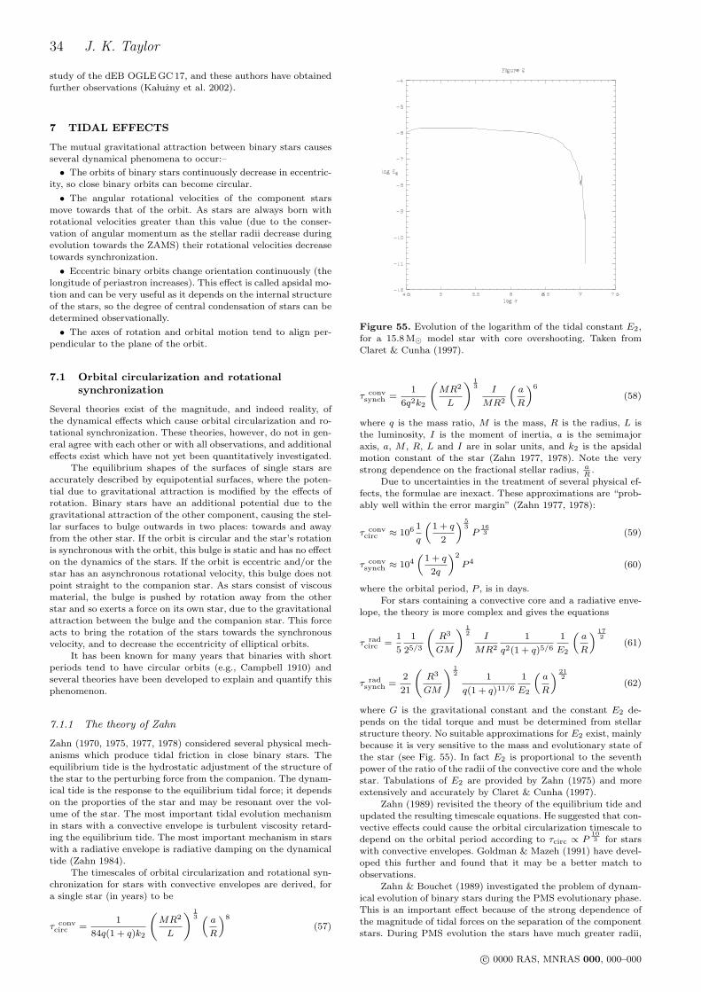
34 J. K. Taylor
study of the dEB OGLE GC 17, and these authors have obtainedfurther observations (KaÃluzny et al. 2002).
7 TIDAL EFFECTS
The mutual gravitational attraction between binary stars causesseveral dynamical phenomena to occur:–
• The orbits of binary stars continuously decrease in eccentric-ity, so close binary orbits can become circular.
• The angular rotational velocities of the component starsmove towards that of the orbit. As stars are always born withrotational velocities greater than this value (due to the conser-vation of angular momentum as the stellar radii decrease duringevolution towards the ZAMS) their rotational velocities decreasetowards synchronization.
• Eccentric binary orbits change orientation continuously (thelongitude of periastron increases). This effect is called apsidal mo-tion and can be very useful as it depends on the internal structureof the stars, so the degree of central condensation of stars can bedetermined observationally.
• The axes of rotation and orbital motion tend to align per-pendicular to the plane of the orbit.
7.1 Orbital circularization and rotationalsynchronization
Several theories exist of the magnitude, and indeed reality, ofthe dynamical effects which cause orbital circularization and ro-tational synchronization. These theories, however, do not in gen-eral agree with each other or with all observations, and additionaleffects exist which have not yet been quantitatively investigated.
The equilibrium shapes of the surfaces of single stars areaccurately described by equipotential surfaces, where the poten-tial due to gravitational attraction is modified by the effects ofrotation. Binary stars have an additional potential due to thegravitational attraction of the other component, causing the stel-lar surfaces to bulge outwards in two places: towards and awayfrom the other star. If the orbit is circular and the star’s rotationis synchronous with the orbit, this bulge is static and has no effecton the dynamics of the stars. If the orbit is eccentric and/or thestar has an asynchronous rotational velocity, this bulge does notpoint straight to the companion star. As stars consist of viscousmaterial, the bulge is pushed by rotation away from the otherstar and so exerts a force on its own star, due to the gravitationalattraction between the bulge and the companion star. This forceacts to bring the rotation of the stars towards the synchronousvelocity, and to decrease the eccentricity of elliptical orbits.
It has been known for many years that binaries with shortperiods tend to have circular orbits (e.g., Campbell 1910) andseveral theories have been developed to explain and quantify thisphenomenon.
7.1.1 The theory of Zahn
Zahn (1970, 1975, 1977, 1978) considered several physical mech-anisms which produce tidal friction in close binary stars. Theequilibrium tide is the hydrostatic adjustment of the structure ofthe star to the perturbing force from the companion. The dynam-ical tide is the response to the equilibrium tidal force; it dependson the proporties of the star and may be resonant over the vol-ume of the star. The most important tidal evolution mechanismin stars with a convective envelope is turbulent viscosity retard-ing the equilibrium tide. The most important mechanism in starswith a radiative envelope is radiative damping on the dynamicaltide (Zahn 1984).
The timescales of orbital circularization and rotational syn-chronization for stars with convective envelopes are derived, fora single star (in years) to be
τ convcirc =
1
84q(1 + q)k2
(MR2
L
) 13 (
a
R
)8
(57)
Figure 55. Evolution of the logarithm of the tidal constant E2,for a 15.8 M¯ model star with core overshooting. Taken fromClaret & Cunha (1997).
τ convsynch =
1
6q2k2
(MR2
L
) 13 I
MR2
(a
R
)6
(58)
where q is the mass ratio, M is the mass, R is the radius, L isthe luminosity, I is the moment of inertia, a is the semimajoraxis, a, M , R, L and I are in solar units, and k2 is the apsidalmotion constant of the star (Zahn 1977, 1978). Note the verystrong dependence on the fractional stellar radius, a
R.
Due to uncertainties in the treatment of several physical ef-fects, the formulae are inexact. These approximations are “prob-ably well within the error margin” (Zahn 1977, 1978):
τ convcirc ≈ 106 1
q
(1 + q
2
) 53P
163 (59)
τ convsynch ≈ 104
(1 + q
2q
)2
P 4 (60)
where the orbital period, P , is in days.
For stars containing a convective core and a radiative enve-lope, the theory is more complex and gives the equations
τ radcirc =
1
5
1
25/3
(R3
GM
) 12 I
MR2
1
q2(1 + q)5/6
1
E2
(a
R
) 172
(61)
τ radsynch =
2
21
(R3
GM
) 12 1
q(1 + q)11/6
1
E2
(a
R
) 212
(62)
where G is the gravitational constant and the constant E2 de-pends on the tidal torque and must be determined from stellarstructure theory. No suitable approximations for E2 exist, mainlybecause it is very sensitive to the mass and evolutionary state ofthe star (see Fig. 55). In fact E2 is proportional to the seventhpower of the ratio of the radii of the convective core and the wholestar. Tabulations of E2 are provided by Zahn (1975) and moreextensively and accurately by Claret & Cunha (1997).
Zahn (1989) revisited the theory of the equilibrium tide andupdated the resulting timescale equations. He suggested that con-vective effects could cause the orbital circularization timescale todepend on the orbital period according to τcirc ∝ P
103 for stars
with convective envelopes. Goldman & Mazeh (1991) have devel-oped this further and found that it may be a better match toobservations.
Zahn & Bouchet (1989) investigated the problem of dynam-ical evolution of binary stars during the PMS evolutionary phase.This is an important effect because of the strong dependence ofthe magnitude of tidal forces on the separation of the componentstars. During PMS evolution the stars have much greater radii,
c© 0000 RAS, MNRAS 000, 000–000
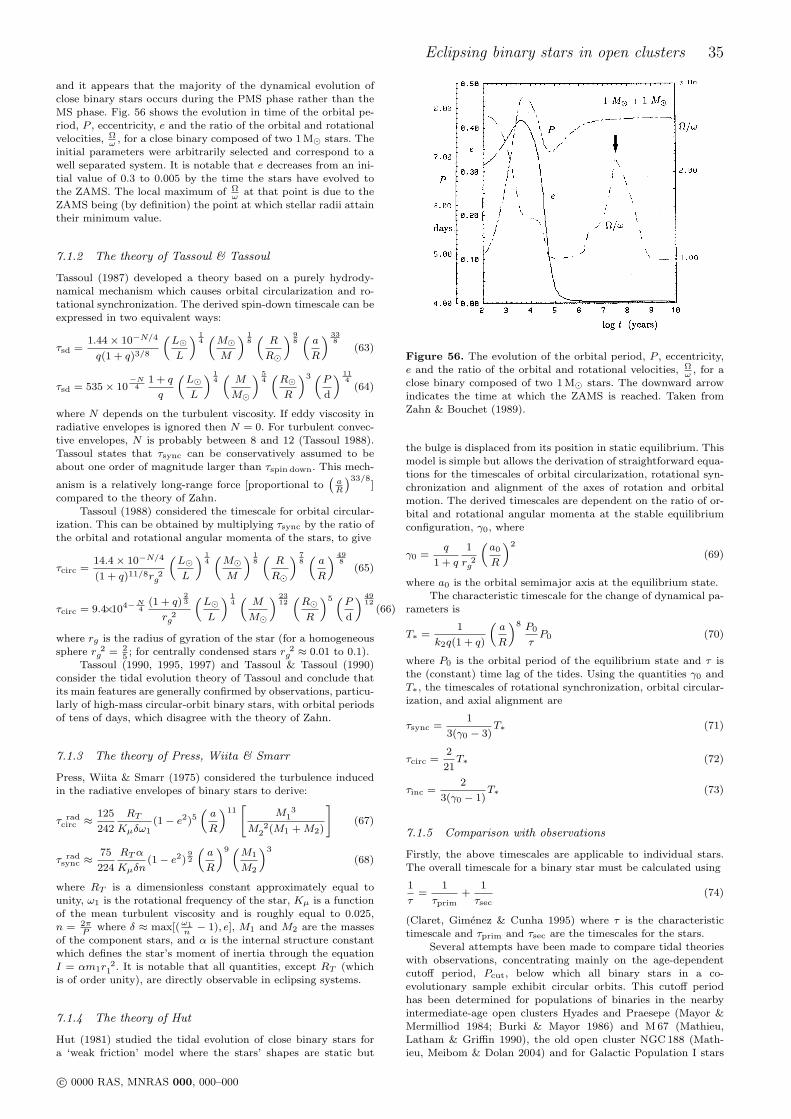
Eclipsing binary stars in open clusters 35
and it appears that the majority of the dynamical evolution ofclose binary stars occurs during the PMS phase rather than theMS phase. Fig. 56 shows the evolution in time of the orbital pe-riod, P , eccentricity, e and the ratio of the orbital and rotationalvelocities, Ω
ω, for a close binary composed of two 1 M¯ stars. The
initial parameters were arbitrarily selected and correspond to awell separated system. It is notable that e decreases from an ini-tial value of 0.3 to 0.005 by the time the stars have evolved tothe ZAMS. The local maximum of Ω
ωat that point is due to the
ZAMS being (by definition) the point at which stellar radii attaintheir minimum value.
7.1.2 The theory of Tassoul & Tassoul
Tassoul (1987) developed a theory based on a purely hydrody-namical mechanism which causes orbital circularization and ro-tational synchronization. The derived spin-down timescale can beexpressed in two equivalent ways:
τsd =1.44× 10−N/4
q(1 + q)3/8
(L¯L
) 14(M¯M
) 18(R
R¯
) 98(a
R
) 338
(63)
τsd = 535× 10−N4
1 + q
q
(L¯L
) 14(M
M¯
) 54(R¯R
)3 (P
d
) 114
(64)
where N depends on the turbulent viscosity. If eddy viscosity inradiative envelopes is ignored then N = 0. For turbulent convec-tive envelopes, N is probably between 8 and 12 (Tassoul 1988).Tassoul states that τsync can be conservatively assumed to beabout one order of magnitude larger than τspin down. This mech-
anism is a relatively long-range force [proportional to(
aR
)33/8]
compared to the theory of Zahn.Tassoul (1988) considered the timescale for orbital circular-
ization. This can be obtained by multiplying τsync by the ratio ofthe orbital and rotational angular momenta of the stars, to give
τcirc =14.4× 10−N/4
(1 + q)11/8r 2g
(L¯L
) 14(M¯M
) 18(R
R¯
) 78(a
R
) 498
(65)
τcirc = 9.4×10⁴−N4
(1 + q)23
r 2g
(L¯L
) 14(M
M¯
) 2312
(R¯R
)5 (P
d
) 4912
(66)
where rg is the radius of gyration of the star (for a homogeneoussphere r 2
g = 25
; for centrally condensed stars r 2g ≈ 0.01 to 0.1).
Tassoul (1990, 1995, 1997) and Tassoul & Tassoul (1990)consider the tidal evolution theory of Tassoul and conclude thatits main features are generally confirmed by observations, particu-larly of high-mass circular-orbit binary stars, with orbital periodsof tens of days, which disagree with the theory of Zahn.
7.1.3 The theory of Press, Wiita & Smarr
Press, Wiita & Smarr (1975) considered the turbulence inducedin the radiative envelopes of binary stars to derive:
τ radcirc ≈ 125
242
RT
Kµδω1(1− e2)5
(a
R
)11[
M 31
M 22 (M1 +M2)
](67)
τ radsync ≈
75
224
RTα
Kµδn(1− e2)
92
(a
R
)9 (M1
M2
)3
(68)
where RT is a dimensionless constant approximately equal tounity, ω1 is the rotational frequency of the star, Kµ is a functionof the mean turbulent viscosity and is roughly equal to 0.025,n = 2π
Pwhere δ ≈ max[( ω1
n− 1), e], M1 and M2 are the masses
of the component stars, and α is the internal structure constantwhich defines the star’s moment of inertia through the equationI = αm1r 2
1 . It is notable that all quantities, except RT (whichis of order unity), are directly observable in eclipsing systems.
7.1.4 The theory of Hut
Hut (1981) studied the tidal evolution of close binary stars fora ‘weak friction’ model where the stars’ shapes are static but
Figure 56. The evolution of the orbital period, P , eccentricity,e and the ratio of the orbital and rotational velocities, Ω
ω, for a
close binary composed of two 1 M¯ stars. The downward arrowindicates the time at which the ZAMS is reached. Taken fromZahn & Bouchet (1989).
the bulge is displaced from its position in static equilibrium. Thismodel is simple but allows the derivation of straightforward equa-tions for the timescales of orbital circularization, rotational syn-chronization and alignment of the axes of rotation and orbitalmotion. The derived timescales are dependent on the ratio of or-bital and rotational angular momenta at the stable equilibriumconfiguration, γ0, where
γ0 =q
1 + q
1
r 2g
(a0
R
)2
(69)
where a0 is the orbital semimajor axis at the equilibrium state.The characteristic timescale for the change of dynamical pa-
rameters is
T∗ =1
k2q(1 + q)
(a
R
)8 P0
τP0 (70)
where P0 is the orbital period of the equilibrium state and τ isthe (constant) time lag of the tides. Using the quantities γ0 andT∗, the timescales of rotational synchronization, orbital circular-ization, and axial alignment are
τsync =1
3(γ0 − 3)T∗ (71)
τcirc =2
21T∗ (72)
τinc =2
3(γ0 − 1)T∗ (73)
7.1.5 Comparison with observations
Firstly, the above timescales are applicable to individual stars.The overall timescale for a binary star must be calculated using
1
τ=
1
τprim+
1
τsec(74)
(Claret, Gimenez & Cunha 1995) where τ is the characteristictimescale and τprim and τsec are the timescales for the stars.
Several attempts have been made to compare tidal theorieswith observations, concentrating mainly on the age-dependentcutoff period, Pcut, below which all binary stars in a co-evolutionary sample exhibit circular orbits. This cutoff periodhas been determined for populations of binaries in the nearbyintermediate-age open clusters Hyades and Praesepe (Mayor &Mermilliod 1984; Burki & Mayor 1986) and M 67 (Mathieu,Latham & Griffin 1990), the old open cluster NGC 188 (Math-ieu, Meibom & Dolan 2004) and for Galactic Population I stars
c© 0000 RAS, MNRAS 000, 000–000
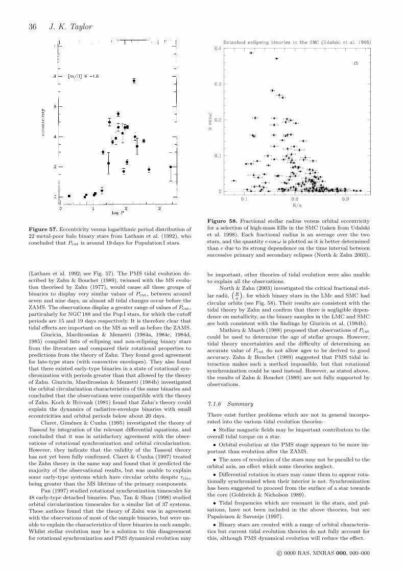
36 J. K. Taylor
Figure 57. Eccentricity versus logarithmic period distribution of22 metal-poor halo binary stars from Latham et al. (1992), whoconcluded that Pcut is around 19 days for Population I stars.
(Latham et al. 1992; see Fig. 57). The PMS tidal evolution de-scribed by Zahn & Bouchet (1989), twinned with the MS evolu-tion theorised by Zahn (1977), would cause all these groups ofbinaries to display very similar values of Pcut, between aroundseven and nine days, as almost all tidal changes occur before theZAMS. The observations display a greater range of values of Pcut,particularly for NGC 188 and the Pop I stars, for which the cutoffperiods are 15 and 19 days respectively. It is therefore clear thattidal effects are important on the MS as well as before the ZAMS.
Giuricin, Mardirossian & Mezzetti (1984a, 1984c, 1984d,1985) compiled lists of eclipsing and non-eclipsing binary starsfrom the literature and compared their rotational properties topredictions from the theory of Zahn. They found good agreementfor late-type stars (with convective envelopes). They also foundthat there existed early-type binaries in a state of rotational syn-chronization with periods greater than that allowed by the theoryof Zahn. Giuricin, Mardirossian & Mezzetti (1984b) investigatedthe orbital circularization characteristics of the same binaries andconcluded that the observations were compatible with the theoryof Zahn. Koch & Hrivnak (1981) found that Zahn’s theory couldexplain the dynamics of radiative-envelope binaries with smalleccentricities and orbital periods below about 20 days.
Claret, Gimenez & Cunha (1995) investigated the theory ofTassoul by integration of the relevant differential equations, andconcluded that it was in satisfactory agreement with the obser-vations of rotational synchronization and orbital circularization.However, they indicate that the validity of the Tassoul theoryhas not yet been fully confirmed. Claret & Cunha (1997) treatedthe Zahn theory in the same way and found that it predicted themajority of the observational results, but was unable to explainsome early-type systems which have circular orbits despite τcircbeing greater than the MS lifetime of the primary components.
Pan (1997) studied rotational synchronization timescales for48 early-type detached binaries. Pan, Tan & Shan (1998) studiedorbital circularization timescales for a similar list of 37 systems.These authors found that the theory of Zahn was in agreementwith the observations of most of the sample binaries, but were un-able to explain the characteristics of three binaries in each sample.Whilst stellar evolution may be a solution to this disagreementfor rotational synchronization and PMS dynamical evolution may
Figure 58. Fractional stellar radius versus orbital eccentricityfor a selection of high-mass EBs in the SMC (taken from Udalskiet al. 1998). Each fractional radius is an average over the twostars, and the quantity e cosω is plotted as it is better determinedthan e due to its strong dependence on the time interval betweensuccessive primary and secondary eclipses (North & Zahn 2003).
be important, other theories of tidal evolution were also unableto explain all the observations.
North & Zahn (2003) investigated the critical fractional stel-
lar radii,(
Ra
), for which binary stars in the LMc and SMC had
circular orbits (see Fig. 58). Their results are consistent with thetidal theory by Zahn and confirm that there is negligible depen-dence on metallicity, as the binary samples in the LMC and SMCare both consistent with the findings by Giuricin et al. (1984b).
Mathieu & Mazeh (1988) proposed that observations of Pcut
could be used to determine the age of stellar groups. However,tidal theory uncertainties and the difficulty of determining anaccurate value of Pcut do not allow ages to be derived to goodaccuracy. Zahn & Bouchet (1989) suggested that PMS tidal in-teraction makes such a method impossible, but that rotationalsynchronization could be used instead. However, as stated above,the results of Zahn & Bouchet (1989) are not fully supported byobservations.
7.1.6 Summary
There exist further problems which are not in general incorpo-rated into the various tidal evolution theories:–
• Stellar magnetic fields may be important contributors to theoverall tidal torque on a star.
• Orbital evolution at the PMS stage appears to be more im-portant than evolution after the ZAMS.
• The axes of revolution of the stars may not be parallel to theorbital axis, an effect which some theories neglect.
• Differential rotation in stars may cause them to appear rota-tionally synchronized when their interior is not. Synchronizationhas been suggested to proceed from the surface of a star towardsthe core (Goldreich & Nicholson 1989).
• Tidal frequencies which are resonant in the stars, and pul-sations, have not been included in the above theories, but seePapaloizou & Savonije (1997).
• Binary stars are created with a range of orbital characteris-tics but current tidal evolution theories do not fully account forthis, although PMS dynamical evolution will reduce the effect.
c© 0000 RAS, MNRAS 000, 000–000
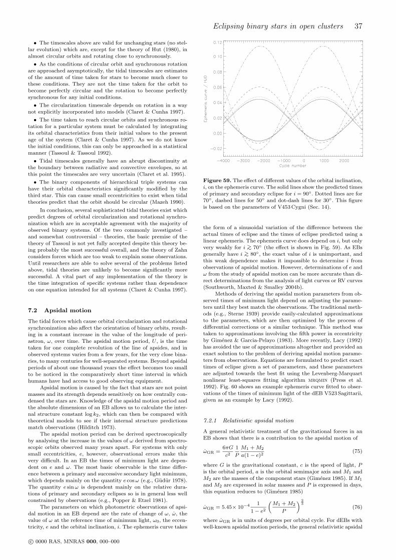
Eclipsing binary stars in open clusters 37
• The timescales above are valid for unchanging stars (no stel-lar evolution) which are, except for the theory of Hut (1980), inalmost circular orbits and rotating close to synchronously.
• As the conditions of circular orbit and synchronous rotationare approached asymptotically, the tidal timescales are estimatesof the amount of time taken for stars to become much closer tothese conditions. They are not the time taken for the orbit tobecome perfectly circular and the rotation to become perfectlysynchronous for any initial conditions.
• The circularization timescale depends on rotation in a waynot explicitly incorporated into models (Claret & Cunha 1997).
• The time taken to reach circular orbits and synchronous ro-tation for a particular system must be calculated by integratingits orbital characteristics from their initial values to the presentage of the system (Claret & Cunha 1997). As we do not knowthe initial conditions, this can only be approached in a statisticalmanner (Tassoul & Tassoul 1992).
• Tidal timescales generally have an abrupt discontinuity atthe boundary between radiative and convective envelopes, so atthis point the timescales are very uncertain (Claret et al. 1995).
• The binary components of hierarchical triple systems canhave their orbital characteristics significantly modified by thethird star. This can cause small eccentricities to exist when tidaltheories predict that the orbit should be circular (Mazeh 1990).
In conclusion, several sophisticated tidal theories exist whichpredict degrees of orbital circularization and rotational synchro-nization which are in acceptable agreement with the majority ofobserved binary systems. Of the two commonly investigated –and somewhat controversial – theories, the basic premise of thetheory of Tassoul is not yet fully accepted despite this theory be-ing probably the most successful overall, and the theory of Zahnconsiders forces which are too weak to explain some observations.Until researchers are able to solve several of the problems listedabove, tidal theories are unlikely to become significantly moresuccessful. A vital part of any implementation of the theory isthe time integration of specific systems rather than dependenceon one equation intended for all systems (Claret & Cunha 1997).
7.2 Apsidal motion
The tidal forces which cause orbital circularization and rotationalsynchronization also affect the orientation of binary orbits, result-ing in a constant increase in the value of the longitude of peri-astron, ω, over time. The apsidal motion period, U , is the timetaken for one complete revolution of the line of apsides, and inobserved systems varies from a few years, for the very close bina-ries, to many centuries for well-separated systems. Beyond apsidalperiods of about one thousand years the effect becomes too smallto be noticed in the comparatively short time interval in whichhumans have had access to good observing equipment.
Apsidal motion is caused by the fact that stars are not pointmasses and its strength depends sensitively on how centrally con-densed the stars are. Knowledge of the apsidal motion period andthe absolute dimensions of an EB allows us to calculate the inter-nal structure constant log k2, which can then be compared withtheoretical models to see if their internal structure predictionsmatch observations (Hilditch 1973).
The apsidal motion period can be derived spectroscopicallyby analysing the increase in the values of ω derived from spectro-scopic orbits observed many years apart. For systems with onlysmall eccentricities, e, however, observational errors make thisvery difficult. In an EB the times of minimum light are depen-dent on e and ω. The most basic observable is the time differ-ence between a primary and successive secondary light minimum,which depends mainly on the quantity e cosω (e.g., Gudur 1978).The quantity e sinω is dependent mainly on the relative dura-tions of primary and secondary eclipses so is in general less wellconstrained by observations (e.g., Popper & Etzel 1981).
The parameters on which photometric observations of apsi-dal motion in an EB depend are the rate of change of ω, ω, thevalue of ω at the reference time of minimum light, ω0, the eccen-tricity, e and the orbital inclination, i. The ephemeris curve takes
Figure 59. The effect of different values of the orbital inclination,i, on the ephemeris curve. The solid lines show the predicted timesof primary and secondary eclipse for i = 90. Dotted lines are for70, dashed lines for 50 and dot-dash lines for 30. This figureis based on the parameters of V453 Cygni (Sec. 14).
the form of a sinusoidal variation of the difference between theactual times of eclipse and the times of eclipse predicted using alinear ephemeris. The ephemeris curve does depend on i, but onlyvery weakly for i >∼ 70 (the effect is shown in Fig. 59). As EBsgenerally have i >∼ 80, the exact value of i is unimportant, andthis weak dependence makes it impossible to determine i fromobservations of apsidal motion. However, determinations of e andω from the study of apsidal motion can be more accurate than di-rect determinations from the analysis of light curves or RV curves(Southworth, Maxted & Smalley 2004b).
Methods of deriving the apsidal motion parameters from ob-served times of minimum light depend on adjusting the parame-ters until they best match the observations. The traditional meth-ods (e.g., Sterne 1939) provide easily-calculated approximationsto the parameters, which are then optimised by the process ofdifferential corrections or a similar technique. This method wastaken to approximations involving the fifth power in eccentricityby Gimenez & Garcia-Pelayo (1983). More recently, Lacy (1992)has avoided the use of approximations altogether and provided anexact solution to the problem of deriving apsidal motion parame-ters from observations. Equations are formulated to predict exacttimes of eclipse given a set of parameters, and these parametersare adjusted towards the best fit using the Levenberg-Marquartnonlinear least-squares fitting algorithm mrqmin (Press et al.1992). Fig. 60 shows an example ephemeris curve fitted to obser-vations of the times of minimum light of the dEB V523 Sagittarii,given as an example by Lacy (1992).
7.2.1 Relativistic apsidal motion
A general relativistic treatment of the gravitational forces in anEB shows that there is a contribution to the apsidal motion of
ωGR =6πG
c21
P
M1 +M2
a(1− e)2(75)
where G is the gravitational constant, c is the speed of light, Pis the orbital period, a is the orbital semimajor axis and M1 andM2 are the masses of the component stars (Gimenez 1985). If M1
and M2 are expressed in solar masses and P is expressed in days,this equation reduces to (Gimenez 1985)
ωGR = 5.45× 10⁻⁴ 1
1− e2
(M1 +M2
P
) 23
(76)
where ωGR is in units of degrees per orbital cycle. For dEBs withwell-known apsidal motion periods, the general relativistic apsidal
c© 0000 RAS, MNRAS 000, 000–000
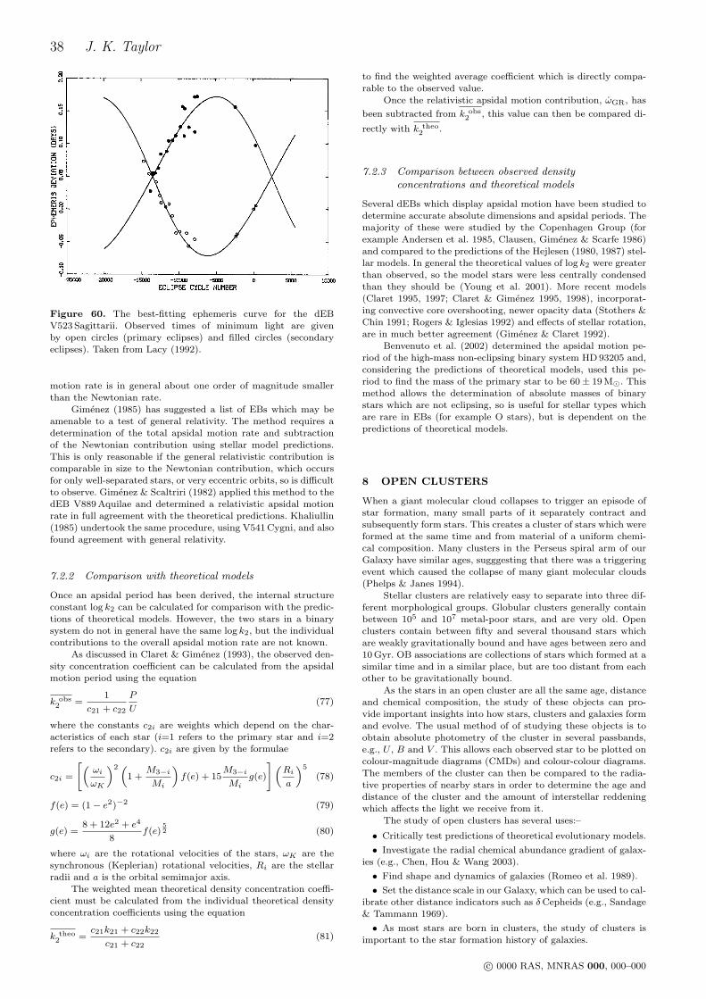
38 J. K. Taylor
Figure 60. The best-fitting ephemeris curve for the dEBV523 Sagittarii. Observed times of minimum light are givenby open circles (primary eclipses) and filled circles (secondaryeclipses). Taken from Lacy (1992).
motion rate is in general about one order of magnitude smallerthan the Newtonian rate.
Gimenez (1985) has suggested a list of EBs which may beamenable to a test of general relativity. The method requires adetermination of the total apsidal motion rate and subtractionof the Newtonian contribution using stellar model predictions.This is only reasonable if the general relativistic contribution iscomparable in size to the Newtonian contribution, which occursfor only well-separated stars, or very eccentric orbits, so is difficultto observe. Gimenez & Scaltriri (1982) applied this method to thedEB V889 Aquilae and determined a relativistic apsidal motionrate in full agreement with the theoretical predictions. Khaliullin(1985) undertook the same procedure, using V541 Cygni, and alsofound agreement with general relativity.
7.2.2 Comparison with theoretical models
Once an apsidal period has been derived, the internal structureconstant log k2 can be calculated for comparison with the predic-tions of theoretical models. However, the two stars in a binarysystem do not in general have the same log k2, but the individualcontributions to the overall apsidal motion rate are not known.
As discussed in Claret & Gimenez (1993), the observed den-sity concentration coefficient can be calculated from the apsidalmotion period using the equation
k obs2 =
1
c21 + c22
P
U(77)
where the constants c2i are weights which depend on the char-acteristics of each star (i=1 refers to the primary star and i=2refers to the secondary). c2i are given by the formulae
c2i =
[(ωi
ωK
)2 (1 +
M3−i
Mi
)f(e) + 15
M3−i
Mig(e)
](Ri
a
)5
(78)
f(e) = (1− e2)−2 (79)
g(e) =8 + 12e2 + e4
8f(e)
52 (80)
where ωi are the rotational velocities of the stars, ωK are thesynchronous (Keplerian) rotational velocities, Ri are the stellarradii and a is the orbital semimajor axis.
The weighted mean theoretical density concentration coeffi-cient must be calculated from the individual theoretical densityconcentration coefficients using the equation
k theo2 =
c21k21 + c22k22
c21 + c22(81)
to find the weighted average coefficient which is directly compa-rable to the observed value.
Once the relativistic apsidal motion contribution, ωGR, has
been subtracted from k obs2 , this value can then be compared di-
rectly with k theo2 .
7.2.3 Comparison between observed densityconcentrations and theoretical models
Several dEBs which display apsidal motion have been studied todetermine accurate absolute dimensions and apsidal periods. Themajority of these were studied by the Copenhagen Group (forexample Andersen et al. 1985, Clausen, Gimenez & Scarfe 1986)and compared to the predictions of the Hejlesen (1980, 1987) stel-lar models. In general the theoretical values of log k2 were greaterthan observed, so the model stars were less centrally condensedthan they should be (Young et al. 2001). More recent models(Claret 1995, 1997; Claret & Gimenez 1995, 1998), incorporat-ing convective core overshooting, newer opacity data (Stothers &Chin 1991; Rogers & Iglesias 1992) and effects of stellar rotation,are in much better agreement (Gimenez & Claret 1992).
Benvenuto et al. (2002) determined the apsidal motion pe-riod of the high-mass non-eclipsing binary system HD 93205 and,considering the predictions of theoretical models, used this pe-riod to find the mass of the primary star to be 60± 19 M¯. Thismethod allows the determination of absolute masses of binarystars which are not eclipsing, so is useful for stellar types whichare rare in EBs (for example O stars), but is dependent on thepredictions of theoretical models.
8 OPEN CLUSTERS
When a giant molecular cloud collapses to trigger an episode ofstar formation, many small parts of it separately contract andsubsequently form stars. This creates a cluster of stars which wereformed at the same time and from material of a uniform chemi-cal composition. Many clusters in the Perseus spiral arm of ourGalaxy have similar ages, sugggesting that there was a triggeringevent which caused the collapse of many giant molecular clouds(Phelps & Janes 1994).
Stellar clusters are relatively easy to separate into three dif-ferent morphological groups. Globular clusters generally containbetween 105 and 107 metal-poor stars, and are very old. Openclusters contain between fifty and several thousand stars whichare weakly gravitationally bound and have ages between zero and10 Gyr. OB associations are collections of stars which formed at asimilar time and in a similar place, but are too distant from eachother to be gravitationally bound.
As the stars in an open cluster are all the same age, distanceand chemical composition, the study of these objects can pro-vide important insights into how stars, clusters and galaxies formand evolve. The usual method of of studying these objects is toobtain absolute photometry of the cluster in several passbands,e.g., U , B and V . This allows each observed star to be plotted oncolour-magnitude diagrams (CMDs) and colour-colour diagrams.The members of the cluster can then be compared to the radia-tive properties of nearby stars in order to determine the age anddistance of the cluster and the amount of interstellar reddeningwhich affects the light we receive from it.
The study of open clusters has several uses:–
• Critically test predictions of theoretical evolutionary models.
• Investigate the radial chemical abundance gradient of galax-ies (e.g., Chen, Hou & Wang 2003).
• Find shape and dynamics of galaxies (Romeo et al. 1989).
• Set the distance scale in our Galaxy, which can be used to cal-ibrate other distance indicators such as δCepheids (e.g., Sandage& Tammann 1969).
• As most stars are born in clusters, the study of clusters isimportant to the star formation history of galaxies.
c© 0000 RAS, MNRAS 000, 000–000
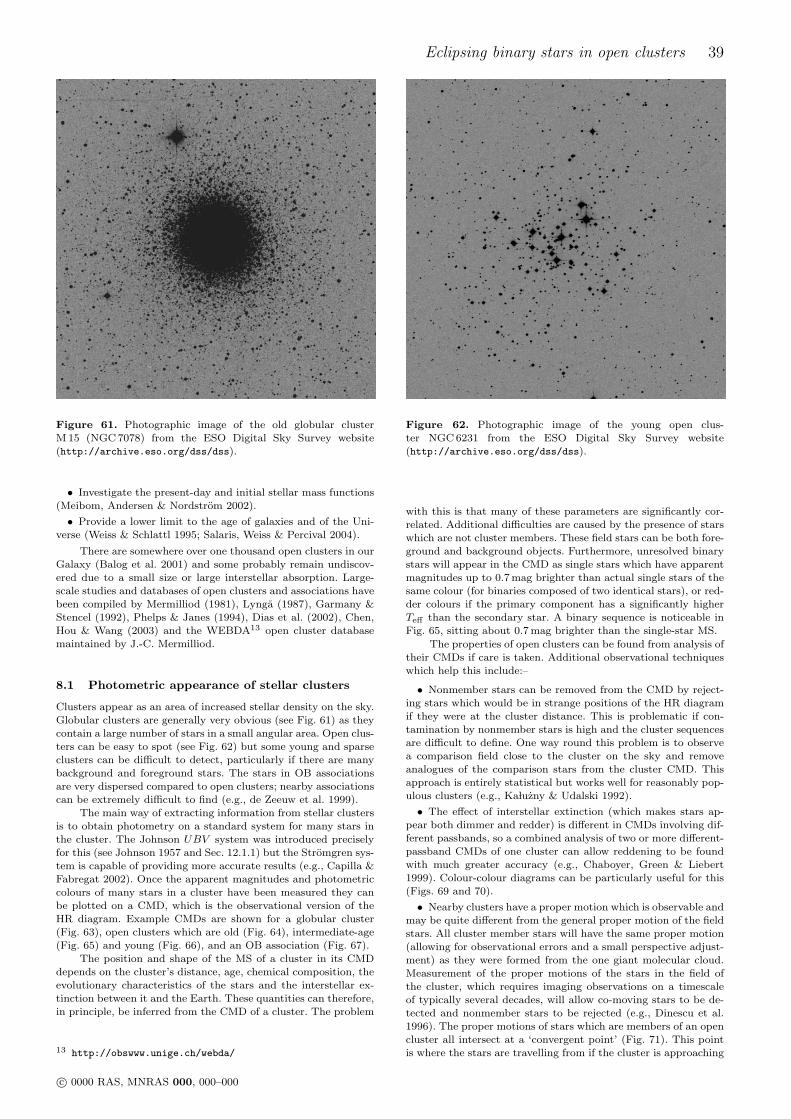
Eclipsing binary stars in open clusters 39
Figure 61. Photographic image of the old globular clusterM 15 (NGC 7078) from the ESO Digital Sky Survey website(http://archive.eso.org/dss/dss).
• Investigate the present-day and initial stellar mass functions(Meibom, Andersen & Nordstrom 2002).
• Provide a lower limit to the age of galaxies and of the Uni-verse (Weiss & Schlattl 1995; Salaris, Weiss & Percival 2004).
There are somewhere over one thousand open clusters in ourGalaxy (Balog et al. 2001) and some probably remain undiscov-ered due to a small size or large interstellar absorption. Large-scale studies and databases of open clusters and associations havebeen compiled by Mermilliod (1981), Lynga (1987), Garmany &Stencel (1992), Phelps & Janes (1994), Dias et al. (2002), Chen,Hou & Wang (2003) and the WEBDA13 open cluster databasemaintained by J.-C. Mermilliod.
8.1 Photometric appearance of stellar clusters
Clusters appear as an area of increased stellar density on the sky.Globular clusters are generally very obvious (see Fig. 61) as theycontain a large number of stars in a small angular area. Open clus-ters can be easy to spot (see Fig. 62) but some young and sparseclusters can be difficult to detect, particularly if there are manybackground and foreground stars. The stars in OB associationsare very dispersed compared to open clusters; nearby associationscan be extremely difficult to find (e.g., de Zeeuw et al. 1999).
The main way of extracting information from stellar clustersis to obtain photometry on a standard system for many stars inthe cluster. The Johnson UBV system was introduced preciselyfor this (see Johnson 1957 and Sec. 12.1.1) but the Stromgren sys-tem is capable of providing more accurate results (e.g., Capilla &Fabregat 2002). Once the apparent magnitudes and photometriccolours of many stars in a cluster have been measured they canbe plotted on a CMD, which is the observational version of theHR diagram. Example CMDs are shown for a globular cluster(Fig. 63), open clusters which are old (Fig. 64), intermediate-age(Fig. 65) and young (Fig. 66), and an OB association (Fig. 67).
The position and shape of the MS of a cluster in its CMDdepends on the cluster’s distance, age, chemical composition, theevolutionary characteristics of the stars and the interstellar ex-tinction between it and the Earth. These quantities can therefore,in principle, be inferred from the CMD of a cluster. The problem
13 http://obswww.unige.ch/webda/
Figure 62. Photographic image of the young open clus-ter NGC 6231 from the ESO Digital Sky Survey website(http://archive.eso.org/dss/dss).
with this is that many of these parameters are significantly cor-related. Additional difficulties are caused by the presence of starswhich are not cluster members. These field stars can be both fore-ground and background objects. Furthermore, unresolved binarystars will appear in the CMD as single stars which have apparentmagnitudes up to 0.7 mag brighter than actual single stars of thesame colour (for binaries composed of two identical stars), or red-der colours if the primary component has a significantly higherTeff than the secondary star. A binary sequence is noticeable inFig. 65, sitting about 0.7 mag brighter than the single-star MS.
The properties of open clusters can be found from analysis oftheir CMDs if care is taken. Additional observational techniqueswhich help this include:–
• Nonmember stars can be removed from the CMD by reject-ing stars which would be in strange positions of the HR diagramif they were at the cluster distance. This is problematic if con-tamination by nonmember stars is high and the cluster sequencesare difficult to define. One way round this problem is to observea comparison field close to the cluster on the sky and removeanalogues of the comparison stars from the cluster CMD. Thisapproach is entirely statistical but works well for reasonably pop-ulous clusters (e.g., KaÃluzny & Udalski 1992).
• The effect of interstellar extinction (which makes stars ap-pear both dimmer and redder) is different in CMDs involving dif-ferent passbands, so a combined analysis of two or more different-passband CMDs of one cluster can allow reddening to be foundwith much greater accuracy (e.g., Chaboyer, Green & Liebert1999). Colour-colour diagrams can be particularly useful for this(Figs. 69 and 70).
• Nearby clusters have a proper motion which is observable andmay be quite different from the general proper motion of the fieldstars. All cluster member stars will have the same proper motion(allowing for observational errors and a small perspective adjust-ment) as they were formed from the one giant molecular cloud.Measurement of the proper motions of the stars in the field ofthe cluster, which requires imaging observations on a timescaleof typically several decades, will allow co-moving stars to be de-tected and nonmember stars to be rejected (e.g., Dinescu et al.1996). The proper motions of stars which are members of an opencluster all intersect at a ‘convergent point’ (Fig. 71). This pointis where the stars are travelling from if the cluster is approaching
c© 0000 RAS, MNRAS 000, 000–000
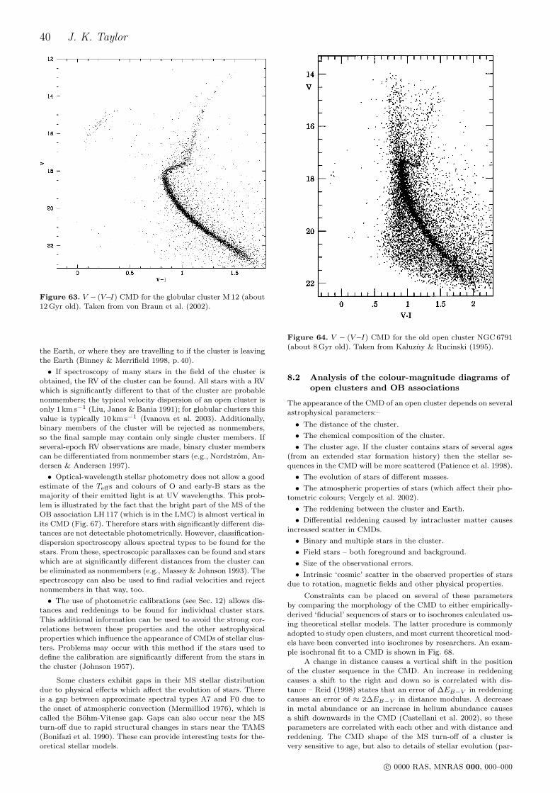
40 J. K. Taylor
Figure 63. V − (V−I) CMD for the globular cluster M 12 (about12 Gyr old). Taken from von Braun et al. (2002).
the Earth, or where they are travelling to if the cluster is leavingthe Earth (Binney & Merrifield 1998, p. 40).
• If spectroscopy of many stars in the field of the cluster isobtained, the RV of the cluster can be found. All stars with a RVwhich is significantly different to that of the cluster are probablenonmembers; the typical velocity dispersion of an open cluster isonly 1 km s−1 (Liu, Janes & Bania 1991); for globular clusters thisvalue is typically 10 km s−1 (Ivanova et al. 2003). Additionally,binary members of the cluster will be rejected as nonmembers,so the final sample may contain only single cluster members. Ifseveral-epoch RV observations are made, binary cluster memberscan be differentiated from nonmember stars (e.g., Nordstrom, An-dersen & Andersen 1997).
• Optical-wavelength stellar photometry does not allow a goodestimate of the Teffs and colours of O and early-B stars as themajority of their emitted light is at UV wavelengths. This prob-lem is illustrated by the fact that the bright part of the MS of theOB association LH 117 (which is in the LMC) is almost vertical inits CMD (Fig. 67). Therefore stars with significantly different dis-tances are not detectable photometrically. However, classification-dispersion spectroscopy allows spectral types to be found for thestars. From these, spectroscopic parallaxes can be found and starswhich are at significantly different distances from the cluster canbe eliminated as nonmembers (e.g., Massey & Johnson 1993). Thespectroscopy can also be used to find radial velocities and rejectnonmembers in that way, too.
• The use of photometric calibrations (see Sec. 12) allows dis-tances and reddenings to be found for individual cluster stars.This additional information can be used to avoid the strong cor-relations between these properties and the other astrophysicalproperties which influence the appearance of CMDs of stellar clus-ters. Problems may occur with this method if the stars used todefine the calibration are significantly different from the stars inthe cluster (Johnson 1957).
Some clusters exhibit gaps in their MS stellar distributiondue to physical effects which affect the evolution of stars. Thereis a gap between approximate spectral types A7 and F0 due tothe onset of atmospheric convection (Mermilliod 1976), which iscalled the Bohm-Vitense gap. Gaps can also occur near the MSturn-off due to rapid structural changes in stars near the TAMS(Bonifazi et al. 1990). These can provide interesting tests for the-oretical stellar models.
Figure 64. V − (V−I) CMD for the old open cluster NGC 6791(about 8 Gyr old). Taken from KaÃluzny & Rucinski (1995).
8.2 Analysis of the colour-magnitude diagrams ofopen clusters and OB associations
The appearance of the CMD of an open cluster depends on severalastrophysical parameters:–
• The distance of the cluster.
• The chemical composition of the cluster.
• The cluster age. If the cluster contains stars of several ages(from an extended star formation history) then the stellar se-quences in the CMD will be more scattered (Patience et al. 1998).
• The evolution of stars of different masses.
• The atmospheric properties of stars (which affect their pho-tometric colours; Vergely et al. 2002).
• The reddening between the cluster and Earth.
• Differential reddening caused by intracluster matter causesincreased scatter in CMDs.
• Binary and multiple stars in the cluster.
• Field stars – both foreground and background.
• Size of the observational errors.
• Intrinsic ‘cosmic’ scatter in the observed properties of starsdue to rotation, magnetic fields and other physical properties.
Constraints can be placed on several of these parametersby comparing the morphology of the CMD to either empirically-derived ‘fiducial’ sequences of stars or to isochrones calculated us-ing theoretical stellar models. The latter procedure is commonlyadopted to study open clusters, and most current theoretical mod-els have been converted into isochrones by researchers. An exam-ple isochronal fit to a CMD is shown in Fig. 68.
A change in distance causes a vertical shift in the positionof the cluster sequence in the CMD. An increase in reddeningcauses a shift to the right and down so is correlated with dis-tance – Reid (1998) states that an error of ∆EB−V in reddeningcauses an error of ≈ 2∆EB−V in distance modulus. A decreasein metal abundance or an increase in helium abundance causesa shift downwards in the CMD (Castellani et al. 2002), so theseparameters are correlated with each other and with distance andreddening. The CMD shape of the MS turn-off of a cluster isvery sensitive to age, but also to details of stellar evolution (par-
c© 0000 RAS, MNRAS 000, 000–000
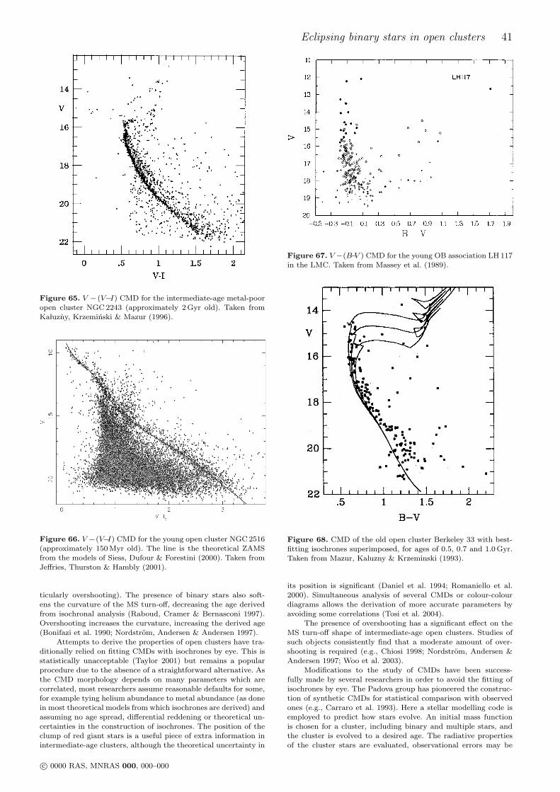
Eclipsing binary stars in open clusters 41
Figure 65. V − (V−I) CMD for the intermediate-age metal-pooropen cluster NGC 2243 (approximately 2 Gyr old). Taken fromKaÃluzny, Krzeminski & Mazur (1996).
Figure 66. V −(V−I) CMD for the young open cluster NGC 2516(approximately 150 Myr old). The line is the theoretical ZAMSfrom the models of Siess, Dufour & Forestini (2000). Taken fromJeffries, Thurston & Hambly (2001).
ticularly overshooting). The presence of binary stars also soft-ens the curvature of the MS turn-off, decreasing the age derivedfrom isochronal analysis (Raboud, Cramer & Bernasconi 1997).Overshooting increases the curvature, increasing the derived age(Bonifazi et al. 1990; Nordstrom, Andersen & Andersen 1997).
Attempts to derive the properties of open clusters have tra-ditionally relied on fitting CMDs with isochrones by eye. This isstatistically unacceptable (Taylor 2001) but remains a popularprocedure due to the absence of a straightforward alternative. Asthe CMD morphology depends on many parameters which arecorrelated, most researchers assume reasonable defaults for some,for example tying helium abundance to metal abundance (as donein most theoretical models from which isochrones are derived) andassuming no age spread, differential reddening or theoretical un-certainties in the construction of isochrones. The position of theclump of red giant stars is a useful piece of extra information inintermediate-age clusters, although the theoretical uncertainty in
Figure 67. V −(B−V ) CMD for the young OB association LH 117in the LMC. Taken from Massey et al. (1989).
Figure 68. CMD of the old open cluster Berkeley 33 with best-fitting isochrones superimposed, for ages of 0.5, 0.7 and 1.0 Gyr.Taken from Mazur, Kaluzny & Krzeminski (1993).
its position is significant (Daniel et al. 1994; Romaniello et al.2000). Simultaneous analysis of several CMDs or colour-colourdiagrams allows the derivation of more accurate parameters byavoiding some correlations (Tosi et al. 2004).
The presence of overshooting has a significant effect on theMS turn-off shape of intermediate-age open clusters. Studies ofsuch objects consistently find that a moderate amount of over-shooting is required (e.g., Chiosi 1998; Nordstrom, Andersen &Andersen 1997; Woo et al. 2003).
Modifications to the study of CMDs have been success-fully made by several researchers in order to avoid the fitting ofisochrones by eye. The Padova group has pioneered the construc-tion of synthetic CMDs for statistical comparison with observedones (e.g., Carraro et al. 1993). Here a stellar modelling code isemployed to predict how stars evolve. An initial mass functionis chosen for a cluster, including binary and multiple stars, andthe cluster is evolved to a desired age. The radiative propertiesof the cluster stars are evaluated, observational errors may be
c© 0000 RAS, MNRAS 000, 000–000
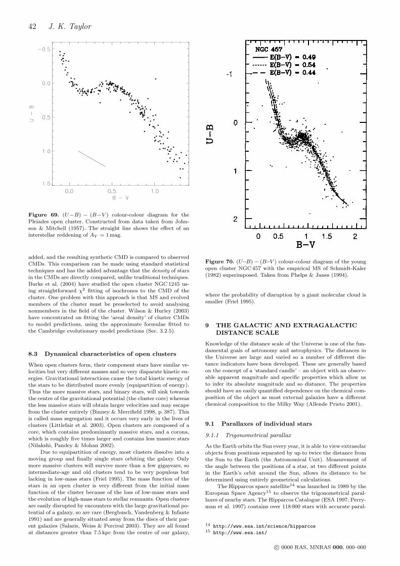
42 J. K. Taylor
Figure 69. (U−B) − (B−V ) colour-colour diagram for thePleiades open cluster. Constructed from data taken from John-son & Mitchell (1957). The straight line shows the effect of aninterstellar reddening of AV = 1 mag.
added, and the resulting synthetic CMD is compared to observedCMDs. This comparison can be made using standard statisticaltechniques and has the added advantage that the density of starsin the CMDs are directly compared, unlike traditional techniques.Burke et al. (2004) have studied the open cluster NGC 1245 us-ing straightforward χ2 fitting of isochrones to the CMD of thecluster. One problem with this approach is that MS and evolvedmembers of the cluster must be preselected to avoid analysingnonmembers in the field of the cluster. Wilson & Hurley (2003)have concentrated on fitting the ‘areal density’ of cluster CMDsto model predictions, using the approximate formulae fitted tothe Cambridge evolutionary model predictions (Sec. 3.2.5).
8.3 Dynamical characteristics of open clusters
When open clusters form, their component stars have similar ve-locities but very different masses and so very disparate kinetic en-ergies. Gravitational interactions cause the total kinetic energy ofthe stars to be distributed more evenly (equipartition of energy).Thus the more massive stars, and binary stars, will sink towardsthe centre of the gravitational potential (the cluster core) whereasthe less massive stars will obtain larger velocities and may escapefrom the cluster entirely (Binney & Merrifield 1998, p. 387). Thisis called mass segregation and it occurs very early in the lives ofclusters (Littlefair et al. 2003). Open clusters are composed of acore, which contains predominantly massive stars, and a corona,which is roughly five times larger and contains less massive stars(Nilakshi, Pandey & Mohan 2002).
Due to equipartition of energy, most clusters dissolve into amoving group and finally single stars orbiting the galaxy. Onlymore massive clusters will survive more than a few gigayears, sointermediate-age and old clusters tend to be very populous butlacking in low-mass stars (Friel 1995). The mass function of thestars in an open cluster is very different from the initial massfunction of the cluster because of the loss of low-mass stars andthe evolution of high-mass stars to stellar remnants. Open clustersare easily disrupted by encounters with the large gravitational po-tential of a galaxy, so are rare (Bergbusch, Vandenberg & Infante1991) and are generally situated away from the discs of their par-ent galaxies (Salaris, Weiss & Percival 2003). They are all foundat distances greater than 7.5 kpc from the centre of our galaxy,
Figure 70. (U−B)− (B−V ) colour-colour diagram of the youngopen cluster NGC 457 with the empirical MS of Schmidt-Kaler(1982) superimposed. Taken from Phelps & Janes (1994).
where the probability of disruption by a giant molecular cloud issmaller (Friel 1995).
9 THE GALACTIC AND EXTRAGALACTICDISTANCE SCALE
Knowledge of the distance scale of the Universe is one of the fun-damental goals of astronomy and astrophysics. The distances inthe Universe are large and varied so a number of different dis-tance indicators have been developed. These are generally basedon the concept of a ‘standard candle’ – an object with an observ-able apparent magnitude and specific properties which allow usto infer its absolute magnitude and so distance. The propertiesshould have an easily quantified dependence on the chemical com-position of the object as most external galaxies have a differentchemical composition to the Milky Way (Allende Prieto 2001).
9.1 Parallaxes of individual stars
9.1.1 Trigonometrical parallax
As the Earth orbits the Sun every year, it is able to view extrasolarobjects from positions separated by up to twice the distance fromthe Sun to the Earth (the Astronomical Unit). Measurement ofthe angle between the positions of a star, at two different pointsin the Earth’s orbit around the Sun, allows its distance to bedetermined using entirely geometrical calculations.
The Hipparcos space satellite14 was launched in 1989 by theEuropean Space Agency15 to observe the trigonometrical paral-laxes of nearby stars. The Hipparcos Catalogue (ESA 1997; Perry-man et al. 1997) contains over 118 000 stars with accurate paral-
14 http://www.esa.int/science/hipparcos15 http://www.esa.int/
c© 0000 RAS, MNRAS 000, 000–000
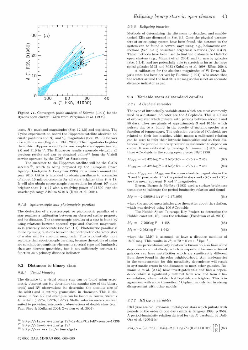
Eclipsing binary stars in open clusters 43
Figure 71. Convergent point analysis of Schwan (1991) for theHyades open cluster. Taken from Perryman et al. (1998).
laxes, HP -passband magnitudes (Sec. 12.1.5) and positions. TheTycho experiment on board the Hipparcos satellite observed ac-curate positions and BT and VT magnitudes (Sec. 12.1.5) for overone million stars (Høg et al. 1998, 2000). The magnitudes brighterthan which Hipparcos and Tycho are complete are approximately8.0 and 11.0 in V . The Hipparcos results supersede virtually allprevious results and can be obtained online16 from the VizieRservice operated by the CDS17 at Strasbourg.
The successor to the Hipparcos satellite will be the GAIAsatellite18, which is being prepared by the European SpaceAgency (Lindegren & Perryman 1996) for a launch around theyear 2010. GAIA is intended to obtain parallaxes to accuraciesof about 10 microarcseconds for all stars brighter than V ≈ 18.It will also obtain spectroscopic observations for about 108 starsbrighter than V ≈ 17 with a resolving power of 11 500 over thewavelength range 8480 to 8740 A (Katz et al. 2004).
9.1.2 Spectroscopic and photometric parallax
The derivation of a spectroscopic or photometric parallax of astar requires a calibration between an observed stellar propertyand its distance. The spectroscopic parallax of a star is found byusing relations between spectral type and absolute magnitude,so is generally inaccurate (see Sec. 1.1). Photometric parallax isfound by using relations between the photometric characteristicsof a star and its absolute magnitude. This is potentially moreaccurate than spectroscopic parallax, because the colours of a starare continuous quantities whereas its spectral type and luminosityclass are discrete quantities, but is not sufficiently accurate tofunction as a primary distance indicator.
9.2 Distances to binary stars
9.2.1 Visual binaries
The distance to a visual binary star can be found using astro-metric observations (to determine the angular size of the binaryorbit) and RV observations (to determine the absolute size ofthe orbit) and is entirely geometrical in character. This is dis-cussed in Sec. 5.2 and examples can be found in Torres, Stefanik& Latham (1997a, 1997b, 1997c). Stellar interferometers are wellsuited to providing astrometric observations of double stars (e.g.,Pan, Shao & Kulkarni 2004; Zwahlen et al. 2004).
16 http://vizier.u-strasbg.fr/viz-bin/VizieR?-source=I/23917 http://cdsweb.u-strasbg.fr/18 http://www.esa.int/science/gaia
9.2.2 Eclipsing binaries
Methods of determining the distances to detached and semide-tached EBs are discussed in Sec. 6.3. Once the physical parame-ters of an eclipsing system have been found, the distance to thesystem can be found in several ways using, e.g., bolometric cor-rections (Sec. 6.3.1) or surface brightness relations (Sec. 6.3.2).These methods have been used to find the distances to Galacticopen clusters (e.g., Munari et al. 2004) and to nearby galaxies(Sec. 6.3.4), and are potentially able to stretch as far as the largespiral galaxies M 31 and M 33 (KaÃluzny et al. 1998; Ribas 2004).
A calibration for the absolute magnitudes of W Ursae Ma-joris stars has been derived by Rucinski (1994), who states thatthe scatter around the best fit is 0.5 mag so this is not an accuratedistance indicator as yet.
9.3 Variable stars as standard candles
9.3.1 δ Cepheid variables
The type of intrinsically-variable stars which are most commonlyused as a distance indicator are the δCepheids. This is a classof evolved star which pulsate with periods between about 1 and50 days. They are giants of approximately 3 and 10 M¯ whichpulsate due to a ‘bump’ in the opacity of metallic species as afunction of temperature. The pulsation periods of δCepheids arerelated to their luminosities, which means a calibrated relationcan be used to infer their intrinsic luminosities and so their dis-tances. The period-luminosity relation is also known to depend oncolour. It was calibrated by Sandage & Tammann (1969), usingthree δCepheids in the young open cluster NGC 7790:
M<V> = −3.425 logP + 2.52(<B> − <V>)− 2.459 (82)
M<B> = −3.425 logP + 3.52(<B> − <V>)− 2.459 (83)
where M<V> and M<B> are the mean absolute magnitudes in theB and V passbands, P is the period in days and <B> and <V>are the mean apparent B and V magnitudes.
Gieren, Barnes & Moffett (1993) used a surface brightnesstechnique to calibrate the period-luminosity relation and found
MV = −2.986(94) logP − 1.371(95) (84)
where the quoted uncertainties give the scatter about the relation,which was derived using 100 δCepheids.
The Hubble Space Telescope Key Project to determine theHubble constant, H0, uses the relations (Freedman et al. 2001)
MV = −2.760 logP − 1.458 (85)
MI = −2.962 logP − 1.942 (86)
where the LMC is assumed to have a distance modulus of18.50 mag. This results in H0 = 72± 8 km s−1 kpc−1.
This period-luminosity relation is known to also have somedependence on metallicity, which is important because externalgalaxies can have metallicities which are significantly differentfrom those found in the solar neighbourhood. Any inadequaciesin the compensation for this metallicity dependence will resultin systematic errors in the distances to most other galaxies. Ro-maniello et al. (2005) have investigated this and find a depen-dence which is significantly different from zero and from a lin-ear relation, where metal-rich δCepheids are brighter. This is inagreement with some theoretical δCepheid models but in strongdisagreement with other models.
9.3.2 RRLyrae variables
RR Lyrae are old, low-mass, metal-poor stars which pulsate withperiods of the order of one day (Zeilik & Gregory 1998, p. 356).A period-luminosity relation derived for the K passband by Dall-Ora et al. (2004) is
<MK>= (−0.770±0.044)−2.101 logP+(0.231±0.012)
[Fe
H
](87)
c© 0000 RAS, MNRAS 000, 000–000
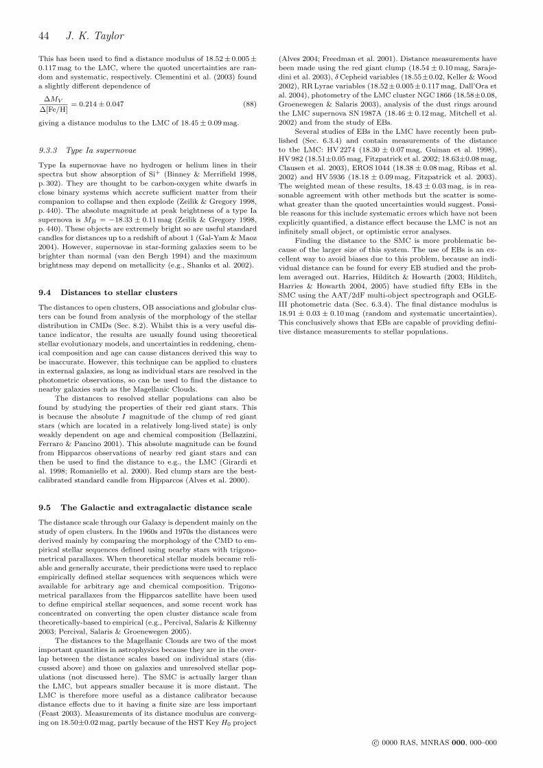
44 J. K. Taylor
This has been used to find a distance modulus of 18.52± 0.005±0.117 mag to the LMC, where the quoted uncertainties are ran-dom and systematic, respectively. Clementini et al. (2003) founda slightly different dependence of
∆MV
∆[Fe/H]= 0.214± 0.047 (88)
giving a distance modulus to the LMC of 18.45± 0.09 mag.
9.3.3 Type Ia supernovae
Type Ia supernovae have no hydrogen or helium lines in theirspectra but show absorption of Si+ (Binney & Merrifield 1998,p. 302). They are thought to be carbon-oxygen white dwarfs inclose binary systems which accrete sufficient matter from theircompanion to collapse and then explode (Zeilik & Gregory 1998,p. 440). The absolute magnitude at peak brightness of a type Iasupernova is MB = −18.33 ± 0.11 mag (Zeilik & Gregory 1998,p. 440). These objects are extremely bright so are useful standardcandles for distances up to a redshift of about 1 (Gal-Yam & Maoz2004). However, supernovae in star-forming galaxies seem to bebrighter than normal (van den Bergh 1994) and the maximumbrightness may depend on metallicity (e.g., Shanks et al. 2002).
9.4 Distances to stellar clusters
The distances to open clusters, OB associations and globular clus-ters can be found from analysis of the morphology of the stellardistribution in CMDs (Sec. 8.2). Whilst this is a very useful dis-tance indicator, the results are usually found using theoreticalstellar evolutionary models, and uncertainties in reddening, chem-ical composition and age can cause distances derived this way tobe inaccurate. However, this technique can be applied to clustersin external galaxies, as long as individual stars are resolved in thephotometric observations, so can be used to find the distance tonearby galaxies such as the Magellanic Clouds.
The distances to resolved stellar populations can also befound by studying the properties of their red giant stars. Thisis because the absolute I magnitude of the clump of red giantstars (which are located in a relatively long-lived state) is onlyweakly dependent on age and chemical composition (Bellazzini,Ferraro & Pancino 2001). This absolute magnitude can be foundfrom Hipparcos observations of nearby red giant stars and canthen be used to find the distance to e.g., the LMC (Girardi etal. 1998; Romaniello et al. 2000). Red clump stars are the best-calibrated standard candle from Hipparcos (Alves et al. 2000).
9.5 The Galactic and extragalactic distance scale
The distance scale through our Galaxy is dependent mainly on thestudy of open clusters. In the 1960s and 1970s the distances werederived mainly by comparing the morphology of the CMD to em-pirical stellar sequences defined using nearby stars with trigono-metrical parallaxes. When theoretical stellar models became reli-able and generally accurate, their predictions were used to replaceempirically defined stellar sequences with sequences which wereavailable for arbitrary age and chemical composition. Trigono-metrical parallaxes from the Hipparcos satellite have been usedto define empirical stellar sequences, and some recent work hasconcentrated on converting the open cluster distance scale fromtheoretically-based to empirical (e.g., Percival, Salaris & Kilkenny2003; Percival, Salaris & Groenewegen 2005).
The distances to the Magellanic Clouds are two of the mostimportant quantities in astrophysics because they are in the over-lap between the distance scales based on individual stars (dis-cussed above) and those on galaxies and unresolved stellar pop-ulations (not discussed here). The SMC is actually larger thanthe LMC, but appears smaller because it is more distant. TheLMC is therefore more useful as a distance calibrator becausedistance effects due to it having a finite size are less important(Feast 2003). Measurements of its distance modulus are converg-ing on 18.50±0.02 mag, partly because of the HST KeyH0 project
(Alves 2004; Freedman et al. 2001). Distance measurements havebeen made using the red giant clump (18.54 ± 0.10 mag, Saraje-dini et al. 2003), δCepheid variables (18.55±0.02, Keller & Wood2002), RR Lyrae variables (18.52±0.005±0.117 mag, Dall’Ora etal. 2004), photometry of the LMC cluster NGC 1866 (18.58±0.08,Groenewegen & Salaris 2003), analysis of the dust rings aroundthe LMC supernova SN 1987A (18.46 ± 0.12 mag, Mitchell et al.2002) and from the study of EBs.
Several studies of EBs in the LMC have recently been pub-lished (Sec. 6.3.4) and contain measurements of the distanceto the LMC: HV 2274 (18.30 ± 0.07 mag, Guinan et al. 1998),HV 982 (18.51±0.05 mag, Fitzpatrick et al. 2002; 18.63±0.08 mag,Clausen et al. 2003), EROS 1044 (18.38 ± 0.08 mag, Ribas et al.2002) and HV 5936 (18.18 ± 0.09 mag, Fitzpatrick et al. 2003).The weighted mean of these results, 18.43 ± 0.03 mag, is in rea-sonable agreement with other methods but the scatter is some-what greater than the quoted uncertainties would suggest. Possi-ble reasons for this include systematic errors which have not beenexplicitly quantified, a distance effect because the LMC is not aninfinitely small object, or optimistic error analyses.
Finding the distance to the SMC is more problematic be-cause of the larger size of this system. The use of EBs is an ex-cellent way to avoid biases due to this problem, because an indi-vidual distance can be found for every EB studied and the prob-lem averaged out. Harries, Hilditch & Howarth (2003; Hilditch,Harries & Howarth 2004, 2005) have studied fifty EBs in theSMC using the AAT/2dF multi-object spectrograph and OGLE-III photometric data (Sec. 6.3.4). The final distance modulus is18.91 ± 0.03 ± 0.10 mag (random and systematic uncertainties).This conclusively shows that EBs are capable of providing defini-tive distance measurements to stellar populations.
c© 0000 RAS, MNRAS 000, 000–000
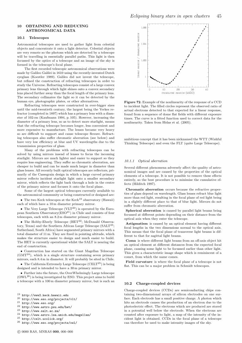
Eclipsing binary stars in open clusters 45
10 OBTAINING AND REDUCINGASTRONOMICAL DATA
10.1 Telescopes
Astronomical telescopes are used to gather light from celestialobjects and concentrate it onto a light detector. Celestial objectsare very remote so the photons which are detected by a telescopewill be travelling in essentially parallel paths. This light is thenfocussed by the optics of a telescope and an image of the sky isformed in the telescope’s focal plane.
The first recorded telescopic astronomical observations weremade by Galileo Galilei in 1610 using the recently-invented Dutcheyeglass (Koestler 1989). Galileo did not invent the telescope,but refined the construction of refracting telescopes in order tostudy the Universe. Refracting telescopes consist of a large convexprimary lens through which light shines onto a convex secondarylens placed further away than the focal length of the primary lens.The secondary collimates the light so it can be detected by thehuman eye, photographic plates, or other alternatives.
Refracting telescopes were constructed in ever-bigger sizesuntil the mid-twentieth century, the largest being the Yerkes re-fractor (completed in 1897) which has a primary lens with a diam-eter of 102 cm (Kaufmann 1994, p. 105). However, increasing thediameter of a primary lens, so as to detect more starlight, meansthat the refracting telescope becomes longer, less convenient andmore expensive to manufacture. The lenses became very heavyso are difficult to support and cause telescope flexure. Refract-ing telescopes also suffer chromatic aberration (see below) andhave very low efficiency at blue and UV wavelengths due to thetransmission properties of glass.
Many of the problems with refracting telescopes can besolved by using mirrors insead of lenses to focus the incomingstarlight. Mirrors are much lighter and easier to support so theyrequire less engineering. They suffer no chromatic aberration, arecheaper to build and can be made much larger in diameter thanglass lenses. All recently built optical telescopes are reflectors, pri-marily of the Cassegrain design in which a large curved primarymirror reflects incident starlight light onto a smaller secondarymirror, which reflects the light back through a hole in the centreof the primary mirror and focuses it onto the focal plane.
Some of the largest optical telescopes currently available tothe astronomical community or being constructed or designed are:
• The two Keck telescopes at the Keck19 observatory (Hawaii)each of which have a 10 m diameter primary mirror.
• The Very Large Telescope (VLT20) is operated by the Euro-pean Southern Observatory(ESO21) in Chile and consists of fourtelescopes, each with an 8.2 m diameter primary mirror.
• The Hobby-Eberly Telescope (HET22; McDonald Observa-tory, Texas) and the Southern African Large Telescope (SALT23;Sutherland, South Africa) have segmented primary mirrors with atotal diameter of 11 m. They are fixed in pointing altitude, whichmakes the structure easier to design and much easier to build.The HET is currently operational whilst the SALT is nearing theend of construction.
• Construction has started on the Giant Magellan Telescope(GMT24), which is a single structure containing seven primarymirrors, each 8.4 m in diameter. It will probably be sited in Chile.
• The California Extremely Large Telescope (CELT25) is beingdesigned and is intended to have a 30 m primary mirror.
• Further into the future, the OverWhelmingly Large telescope(OWL26) is being investigated by ESO. This project aims to builda telescope with a 100 m diameter primary mirror, but is such an
19 http://www2.keck.hawaii.edu20 http://www.eso.org/projects/vlt/21 http://www.eso.org/22 http://www.astro.psu.edu/het/23 http://www.salt.ac.za/24 http://www.astro.lsa.umich.edu/magellan/25 http://celt.ucolick.org/26 http://www.eso.org/projects/owl/
Figure 72. Example of the nonlinearity of the response of a CCDto incident light. The filled circles represent the observed ratio ofactual electrons detected to that expected for a linear response,found from a sequence of dome flat fields with different exposuretimes. The curve is a fitted function used to correct data for thenonlinearity. Taken from Hidas et al. (2005).
ambitious concept that it has been nicknamed the WTT (WishfulThinking Telescope) and even the FLT (quite Large Telescope).
10.1.1 Optical aberration
Several different phenomena adversely affect the quality of astro-nomical images and are caused by the properties of the opticalelements of a telescope. It is not possible to remove these effectsentirely, so the best procedure is to minimise the cumulative ef-fects (Hilditch 1997).
Chromatic aberration occurs because the refractive proper-ties of glass depend on wavelength. Glass lenses refract blue lightmore than red light, resulting in the focal plane of red light beingin a slightly different place to that of blue light. Mirrors do notsuffer from chromatic aberration.
Spherical aberration is caused by parallel light beams beingfocussed at different points depending on their distance from theoptical axis when they enter the telescope.
Astigmatism is caused by an optical element having differentfocal lengths in the two dimensions normal to the optical axis.This means that the focal plane of transverse light beams is dif-ferent to that for sagittal light beams.
Coma is where different light beams from an off-axis object hitan optical element at different distances from the expected focalplane, causing some light to be focussed earlier than other light.This gives a characteristic image shape which is reminiscent of acomet, from which the name comes.
Field curvature is where the focal plane of a telescope is notflat. This can be a major problem in Schmidt telescopes.
10.2 Charge-coupled devices
Charge-coupled devices (CCDs) are semiconducting chips con-taining two-dimensional arrays of silicon electrodes on one sur-face. Each electrode has a small positive charge. A photon whichhits an electrode causes the production of an electron due to thephotoelectric effect. The electrons which are produced are storedin a potential well below the electrode. When the electrons arecounted after exposure to light, a map of the intensity of the in-cident light is obtained. CCDs in the focal plane of a telescopecan therefore be used to make intensity images of the sky.
c© 0000 RAS, MNRAS 000, 000–000
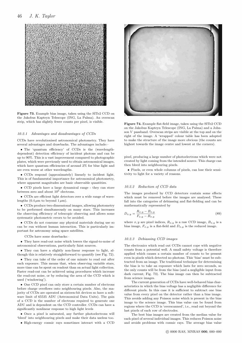
46 J. K. Taylor
Figure 73. Example bias image, taken using the SITe2 CCD onthe Jakobus Kapteyn Telescope (ING, La Palma). An overscanstrip, which has slightly fewer counts per pixel, is visible.
10.2.1 Advantages and disadvantages of CCDs
CCDs have revolutionised astronomical photometry. They haveseveral advantages and drawbacks. The advantages include:–
• The ‘quantum efficiency’ of CCDs is the (wavelength-dependent) detection efficiency of incident photons and can beup to 90%. This is a vast improvement compared to photographicplates, which were previously used to obtain astronomical images,which have quantum efficiencies of around 2% for blue light andare even worse at other wavelengths.
• CCDs respond (approximately) linearly to incident light.This is of fundamental importance for astronomical photometry,where apparent magnitudes are basic observable quantities.
• CCD pixels have a large dynamical range - they can storebetween zero and about 105 electrons.
• CCDs are efficient light detectors over a wide range of wave-lengths (0.4µm to beyond 1µm).
• CCDs produce two-dimensional images, allowing photometryto be performed simultaneously on many stars. This increasesthe observing efficiency of telescopic observing and allows somesystematic photometric errors to be avoided.
• CCDs do not consume any physical materials during use socan be run without human interaction. This is particularly im-portant for astronomy using space satellites.
CCDs have some drawbacks:–
• They have read-out noise which lowers the signal-to-noise ofastronomical observations, particularly faint sources.
• They can have a slightly non-linear response to light, al-though this is relatively straightforward to quantify (see Fig. 72).
• They can take of the order of one minute to read out aftereach exposure. This means that, when observing variable stars,more time can be spent on readout than on actual light collection.Faster read-out can be achieved using procedures which increasethe read-out noise, or by reducing the area of the CCD which isused (‘windowing’).
• One CCD pixel can only store a certain number of electronsbefore charge overflows onto neighbouring pixels. Also, the ma-jority of CCDs are operated as sixteen-bit devices so have a soft-ware limit of 65535 ADU (Astronomical Data Units). The gainof a CCD is the number of electrons required to generate oneADU and is dependent on the CCD controller. CCDs can have asignificantly nonlinear response to high light levels
• Once a pixel is saturated, any further photoelectrons will‘bleed’ into neighbouring pixels and make their data useless too.
• High-energy cosmic rays sometimes interact with a CCD
Figure 74. Example flat-field image, taken using the SITe2 CCDon the Jakobus Kapteyn Telescope (ING, La Palma) and a John-son V passband. Overscan strips are visible at the top and on theright of the image. A ‘wrapped’ colour table has been adoptedto make the structure of the image more obvious (the counts arehighest towards the image centre and lowest at the corners).
pixel, producing a large number of photoelectrons which were notcreated by light coming from the intended source. This charge canthen bleed into neighbouring pixels.
• Pixels, or even whole columns of pixels, can lose their sensi-tivity to light for a variety of reasons.
10.2.2 Reduction of CCD data
The images produced by CCD detectors contain some effectswhich must be removed before the images are analysed. Thesefall into the categories of debiassing and flat-fielding and can bemathematically represented by
Dx,y =Rx,y −Bx,y
Fx,y −Bx,y(89)
where x, y are pixel indices, Rx,y is a raw CCD image, Bx,y is abias image, Fx,y is a flat-field and Dx,y is the reduced image.
10.2.3 Debiassing CCD images
The electronics which read out CCDs cannot cope with negativecounts from a potential well. A small safety voltage is thereforeapplied which causes a certain number of counts to be presenteven in pixels which detected no photons. This ‘bias’ must be sub-tracted from an image. The traditional technique for determiningthe bias is to take an exposure which lasts for zero seconds, sothe only counts will be from the bias (and a negligible input fromdark current; Fig. 73). The bias image can then be subtractedfrom science images.
The current generation of CCDs have well-behaved bias char-acteristics in which the bias voltage has a negligible difference fordifferent pixels. In this case it is sufficient to subtract one biasvalue from every pixel on the detector rather than a bias image.This avoids adding any Poisson noise which is present in the biasimage to the science image. This bias value can be found fromregions where the CCD is ‘overscanned’, i.e., read out beyond thelast pixels of each row of electrodes.
The best bias images are created from the median value foreach pixel of several individual images. This reduces Poisson noiseand avoids problems with cosmic rays. The average bias value
c© 0000 RAS, MNRAS 000, 000–000
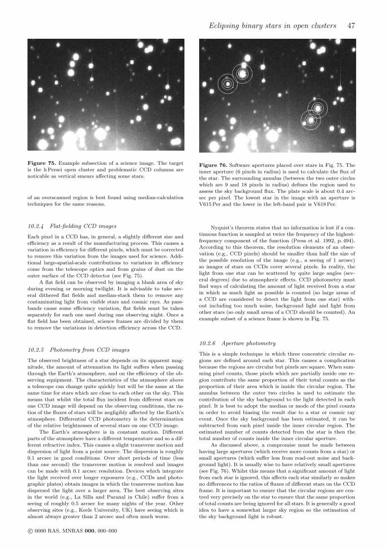
Eclipsing binary stars in open clusters 47
Figure 75. Example subsection of a science image. The targetis the h Persei open cluster and problematic CCD columns arenoticable as vertical smears affecting some stars.
of an overscanned region is best found using median-calculationtechniques for the same reasons.
10.2.4 Flat-fielding CCD images
Each pixel in a CCD has, in general, a slightly different size andefficiency as a result of the manufacturing process. This causes avariation in efficiency for different pixels, which must be correctedto remove this variation from the images used for science. Addi-tional large-spatial-scale contributions to variation in efficiencycome from the telescope optics and from grains of dust on theouter surface of the CCD detector (see Fig. 75).
A flat field can be observed by imaging a blank area of skyduring evening or morning twilight. It is advisable to take sev-eral dithered flat fields and median-stack them to remove anycontaminating light from visible stars and cosmic rays. As pass-bands cause some efficiency variation, flat fields must be takenseparately for each one used during one observing night. Once aflat field has been obtained, science frames are divided by themto remove the variations in detection efficiency across the CCD.
10.2.5 Photometry from CCD images
The observed brightness of a star depends on its apparent mag-nitude, the amount of attenuation its light suffers when passingthrough the Earth’s atmosphere, and on the efficiency of the ob-serving equipment. The characteristics of the atmosphere abovea telescope can change quite quickly but will be the same at thesame time for stars which are close to each other on the sky. Thismeans that whilst the total flux incident from different stars onone CCD image will depend on the observing conditions, the ra-tios of the fluxes of stars will be negligibly affected by the Earth’satmosphere. Differential CCD photometry is the determinationof the relative brightnesses of several stars on one CCD image.
The Earth’s atmosphere is in constant motion. Differentparts of the atmosphere have a different temperature and so a dif-ferent refractive index. This causes a slight transverse motion anddispersion of light from a point source. The dispersion is roughly0.1 arcsec in good conditions. Over short periods of time (lessthan one second) the transverse motion is resolved and imagescan be made with 0.1 arcsec resolution. Devices which integratethe light received over longer exposures (e.g., CCDs and photo-graphic plates) obtain images in which the transverse motion hasdispersed the light over a larger area. The best observing sitesin the world (e.g., La Silla and Paranal in Chile) suffer from aseeing of roughly 0.5 arcsec for many nights of the year. Otherobserving sites (e.g., Keele University, UK) have seeing which isalmost always greater than 2 arcsec and often much worse.
Figure 76. Software apertures placed over stars in Fig. 75. Theinner aperture (6 pixels in radius) is used to calculate the flux ofthe star. The surrounding annulus (between the two outer circleswhich are 9 and 18 pixels in radius) defines the region used toassess the sky background flux. The plate scale is about 0.4 arc-sec per pixel. The lowest star in the image with an aperture isV615 Per and the lower in the left-hand pair is V618 Per.
Nyquist’s theorem states that no information is lost if a con-tinuous function is sampled at twice the frequency of the highest-frequency component of the function (Press et al. 1992, p. 494).According to this theorem, the resolution elements of an obser-vation (e.g., CCD pixels) should be smaller than half the size ofthe possible resolution of the image (e.g., a seeing of 1 arcsec)so images of stars on CCDs cover several pixels. In reality, thelight from one star can be scattered by quite large angles (sev-eral degrees) due to atmospheric effects. CCD photometry mustfind ways of calculating the amount of light received from a starin which as much light as possible is counted (so large areas ofa CCD are considered to detect the light from one star) with-out including too much noise, background light and light fromother stars (so only small areas of a CCD should be counted). Anexample subset of a science frame is shown in Fig. 75.
10.2.6 Aperture photometry
This is a simple technique in which three concentric circular re-gions are defined around each star. This causes a complicationbecause the regions are circular but pixels are square. When sum-ming pixel counts, those pixels which are partially inside one re-gion contribute the same proportion of their total counts as theproportion of their area which is inside the circular region. Theannulus between the outer two circles is used to estimate thecontribution of the sky background to the light detected in eachpixel. It is best to adopt the median or mode of the pixel countsin order to avoid biasing the result due to a star or cosmic rayevent. Once the sky background has been estimated, it can besubtracted from each pixel inside the inner circular region. Theestimated number of counts detected from the star is then thetotal number of counts inside the inner circular aperture.
As discussed above, a compromise must be made betweenhaving large apertures (which receive more counts from a star) orsmall apertures (which suffer less from read-out noise and back-ground light). It is usually wise to have relatively small apertures(see Fig. 76). Whilst this means that a significant amount of lightfrom each star is ignored, this affects each star similarly so makesno differences to the ratios of fluxes of different stars on the CCDframe. It is important to ensure that the circular regions are cen-tred very precisely on the star to ensure that the same proportionof total counts are being ignored for all stars. It is generally a goodidea to have a somewhat larger sky region so the estimation ofthe sky background light is robust.
c© 0000 RAS, MNRAS 000, 000–000
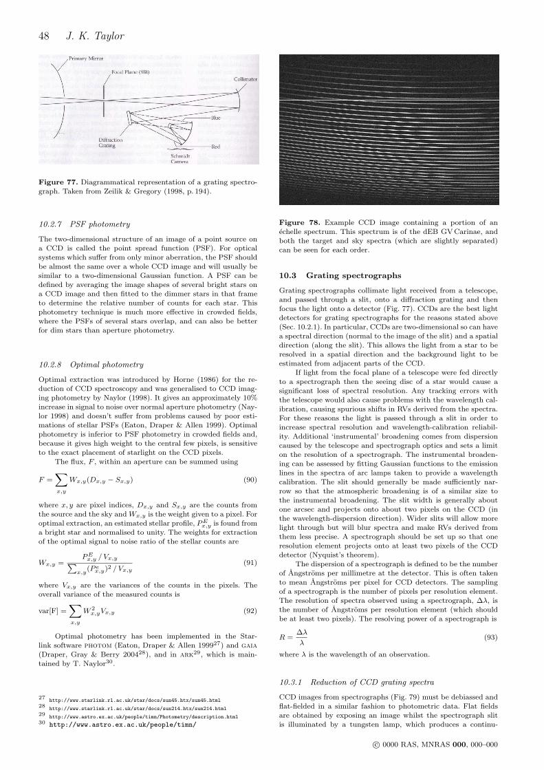
48 J. K. Taylor
Figure 77. Diagrammatical representation of a grating spectro-graph. Taken from Zeilik & Gregory (1998, p. 194).
10.2.7 PSF photometry
The two-dimensional structure of an image of a point source ona CCD is called the point spread function (PSF). For opticalsystems which suffer from only minor aberration, the PSF shouldbe almost the same over a whole CCD image and will usually besimilar to a two-dimensional Gaussian function. A PSF can bedefined by averaging the image shapes of several bright stars ona CCD image and then fitted to the dimmer stars in that frameto determine the relative number of counts for each star. Thisphotometry technique is much more effective in crowded fields,where the PSFs of several stars overlap, and can also be betterfor dim stars than aperture photometry.
10.2.8 Optimal photometry
Optimal extraction was introduced by Horne (1986) for the re-duction of CCD spectroscopy and was generalised to CCD imag-ing photometry by Naylor (1998). It gives an approximately 10%increase in signal to noise over normal aperture photometry (Nay-lor 1998) and doesn’t suffer from problems caused by poor esti-mations of stellar PSFs (Eaton, Draper & Allen 1999). Optimalphotometry is inferior to PSF photometry in crowded fields and,because it gives high weight to the central few pixels, is sensitiveto the exact placement of starlight on the CCD pixels.
The flux, F , within an aperture can be summed using
F =∑x,y
Wx,y(Dx,y − Sx,y) (90)
where x, y are pixel indices, Dx,y and Sx,y are the counts fromthe source and the sky and Wx,y is the weight given to a pixel. Foroptimal extraction, an estimated stellar profile, PE
x,y is found froma bright star and normalised to unity. The weights for extractionof the optimal signal to noise ratio of the stellar counts are
Wx,y =PE
x,y / Vx,y∑x,y
(P ex,y)2 / Vx,y
(91)
where Vx,y are the variances of the counts in the pixels. Theoverall variance of the measured counts is
var[F] =∑x,y
W 2x,yVx,y (92)
Optimal photometry has been implemented in the Star-link software photom (Eaton, Draper & Allen 199927) and gaia(Draper, Gray & Berry 200428), and in ark29, which is main-tained by T. Naylor30.
27http://www.starlink.rl.ac.uk/star/docs/sun45.htx/sun45.html
28http://www.starlink.rl.ac.uk/star/docs/sun214.htx/sun214.html
29http://www.astro.ex.ac.uk/people/timn/Photometry/description.html
30 http://www.astro.ex.ac.uk/people/timn/
Figure 78. Example CCD image containing a portion of anechelle spectrum. This spectrum is of the dEB GV Carinae, andboth the target and sky spectra (which are slightly separated)can be seen for each order.
10.3 Grating spectrographs
Grating spectrographs collimate light received from a telescope,and passed through a slit, onto a diffraction grating and thenfocus the light onto a detector (Fig. 77). CCDs are the best lightdetectors for grating spectrographs for the reasons stated above(Sec. 10.2.1). In particular, CCDs are two-dimensional so can havea spectral direction (normal to the image of the slit) and a spatialdirection (along the slit). This allows the light from a star to beresolved in a spatial direction and the background light to beestimated from adjacent parts of the CCD.
If light from the focal plane of a telescope were fed directlyto a spectrograph then the seeing disc of a star would cause asignificant loss of spectral resolution. Any tracking errors withthe telescope would also cause problems with the wavelength cal-ibration, causing spurious shifts in RVs derived from the spectra.For these reasons the light is passed through a slit in order toincrease spectral resolution and wavelength-calibration reliabil-ity. Additional ‘instrumental’ broadening comes from dispersioncaused by the telescope and spectrograph optics and sets a limiton the resolution of a spectrograph. The instrumental broaden-ing can be assessed by fitting Gaussian functions to the emissionlines in the spectra of arc lamps taken to provide a wavelengthcalibration. The slit should generally be made sufficiently nar-row so that the atmospheric broadening is of a similar size tothe instrumental broadening. The slit width is generally aboutone arcsec and projects onto about two pixels on the CCD (inthe wavelength-dispersion direction). Wider slits will allow morelight through but will blur spectra and make RVs derived fromthem less precise. A spectrograph should be set up so that oneresolution element projects onto at least two pixels of the CCDdetector (Nyquist’s theorem).
The dispersion of a spectrograph is defined to be the numberof Angstroms per millimetre at the detector. This is often takento mean Angstroms per pixel for CCD detectors. The samplingof a spectrograph is the number of pixels per resolution element.The resolution of spectra observed using a spectrograph, ∆λ, isthe number of Angstroms per resolution element (which shouldbe at least two pixels). The resolving power of a spectrograph is
R =∆λ
λ(93)
where λ is the wavelength of an observation.
10.3.1 Reduction of CCD grating spectra
CCD images from spectrographs (Fig. 79) must be debiassed andflat-fielded in a similar fashion to photometric data. Flat fieldsare obtained by exposing an image whilst the spectrograph slitis illuminated by a tungsten lamp, which produces a continu-
c© 0000 RAS, MNRAS 000, 000–000
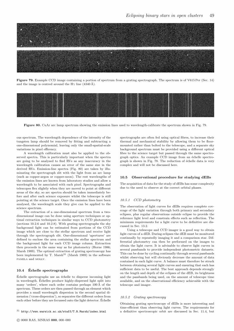
Eclipsing binary stars in open clusters 49
Figure 79. Example CCD image containing a portion of spectrum from a grating spectrograph. The spectrum is of V615 Per (Sec. 14)and the image is centred around the Hγ line (4340 A).
Figure 80. CuAr arc lamp spectrum showing the emission lines used to wavelength-calibrate the spectrum shown in Fig. 79.
ous spectrum. The wavelength dependence of the intensity of thetungsten lamp should be removed by fitting and subtracting aone-dimensional polynomial, leaving only the small-spatial-scalevariations in pixel efficency.
A wavelength calibration must also be applied to the ob-served spectra. This is particularly important when the spectraare going to be analysed to find RVs as any inaccuracy in thewavelength calibration causes an error of the same size in thederived RVs. Emission-line spectra (Fig. 80) are taken by illu-minating the spectrograph slit with the light from an arc lamp(such as copper-argon or copper-neon). The rest wavelengths ofthe emission lines are known from laboratory studies and allow awavelength to be associated with each pixel. Spectrographs andtelescopes flex slightly when they are moved to point at differentareas of the sky, so arc spectra should be taken immediately be-fore and after each science exposure whilst the telescope is stillpointing at the science target. Once the emission lines have beenanalysed, the wavelength scale they give can be applied to thescience spectrum.
The extraction of a one-dimensional spectrum from a two-dimensional image can be done using aperture techniques or op-timal extraction techniques in similar ways to CCD photometry(sections 10.2.6 and 10.2.8). With grating spectrographs the skybackground light can be estimated from portions of the CCDimage which are close to the stellar spectrum and receive lightthrough the spectrograph slit. One-dimensional ‘apertures’ aredefined to enclose the area containing the stellar spectrum andthe background light for each CCD image column. Extractionthen proceeds in the same way as for photometry (Horne 1986;Marsh 1989). The optimal extraction of grating spectroscopy hasbeen implemented by T. Marsh31 (Marsh 1989) in the softwarepamela and molly.
10.4 Echelle spectrographs
Echelle spectrographs use an echelle to disperse incoming lightin wavelength. Echelles produce highly-dispersed light split intomany ‘orders’, where each order contains perhaps 100 A of thespectrum. These orders are then passed through an element whichprovides a small wavelength dispersion in the second spatial di-mension (‘cross-dispersion’), so separates the different orders fromeach other before they are focussed onto the light detector. Echelle
31 http://www.warwick.ac.uk/staff/T.R.Marsh/index.html
spectrographs are often fed using optical fibres, to increase theirthermal and mechanical stability by allowing them to be floor-mounted rather than bolted to the telescope, and a separate skybackground spectrum must be provided using a different opticalfibre to the science target but passed through the same spectro-graph optics. An example CCD image from an echelle spectro-graph is shown in Fig. 78. The reduction of echelle data is verycomplex and will not be discussed here.
10.5 Observational procedure for studying dEBs
The acquisition of data for the study of dEBs has some complexitydue to the need to observe at the correct orbital phases.
10.5.1 CCD photometry
The observation of light curves for dEBs requires complete cov-erage of the light variation through both primary and secondaryeclipses, plus regular observations outside eclipse to provide thereference light level and constrain effects such as reflection. Theminimum requirements for a light curve to be definitive are dis-cussed in Sec. 13.2.
Using a telescope and CCD imager is a good way to obtainlight curves of a dEB. During eclipses the dEB must be monitoredcontinually by repeatedly imaging it and a comparison star. Dif-ferential photometry can then be performed on the images toobtain the light curve. It is advisable to observe light curves inseveral passbands to provide independent photometric datasets.This can be done by cycling continually through several passbandswhilst observing but will obviously decrease the amount of datacontained in each light curve. A balance must therefore be struckbetween obtaining several light curves and ensuring that each hassufficient data to be useful. The best approach depends stronglyon the length and depth of the eclipses of the dEB, its brightnessand the passbands being used, on the amount of telescope timeavailable, and on the observational efficiency achievable with thetelescope and imager.
10.5.2 Grating spectroscopy
Obtaining grating spectroscopy of dEBs is more interesting andtime-efficient than observing light curves. The requirements fora definitive spectroscopic orbit are discussed in Sec. 11.4, but
c© 0000 RAS, MNRAS 000, 000–000
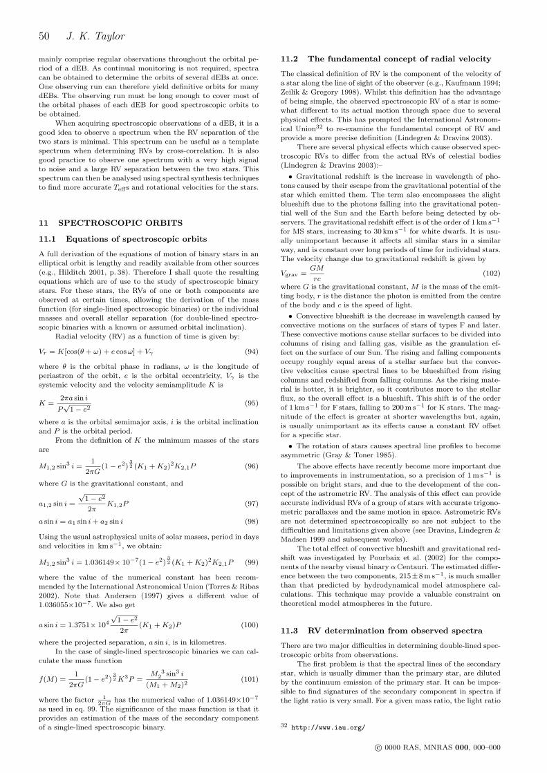
50 J. K. Taylor
mainly comprise regular observations throughout the orbital pe-riod of a dEB. As continual monitoring is not required, spectracan be obtained to determine the orbits of several dEBs at once.One observing run can therefore yield definitive orbits for manydEBs. The observing run must be long enough to cover most ofthe orbital phases of each dEB for good spectroscopic orbits tobe obtained.
When acquiring spectroscopic observations of a dEB, it is agood idea to observe a spectrum when the RV separation of thetwo stars is minimal. This spectrum can be useful as a templatespectrum when determining RVs by cross-correlation. It is alsogood practice to observe one spectrum with a very high signalto noise and a large RV separation between the two stars. Thisspectrum can then be analysed using spectral synthesis techniquesto find more accurate Teffs and rotational velocities for the stars.
11 SPECTROSCOPIC ORBITS
11.1 Equations of spectroscopic orbits
A full derivation of the equations of motion of binary stars in anelliptical orbit is lengthy and readily available from other sources(e.g., Hilditch 2001, p. 38). Therefore I shall quote the resultingequations which are of use to the study of spectroscopic binarystars. For these stars, the RVs of one or both components areobserved at certain times, allowing the derivation of the massfunction (for single-lined spectroscopic binaries) or the individualmasses and overall stellar separation (for double-lined spectro-scopic binaries with a known or assumed orbital inclination).
Radial velocity (RV) as a function of time is given by:
Vr = K[cos(θ + ω) + e cosω] + Vγ (94)
where θ is the orbital phase in radians, ω is the longitude ofperiastron of the orbit, e is the orbital eccentricity, Vγ is thesystemic velocity and the velocity semiamplitude K is
K =2πa sin i
P√
1− e2(95)
where a is the orbital semimajor axis, i is the orbital inclinationand P is the orbital period.
From the definition of K the minimum masses of the starsare
M1,2 sin3 i =1
2πG(1− e2)
32 (K1 +K2)2K2,1P (96)
where G is the gravitational constant, and
a1,2 sin i =
√1− e2
2πK1,2P (97)
a sin i = a1 sin i+ a2 sin i (98)
Using the usual astrophysical units of solar masses, period in daysand velocities in km s−1, we obtain:
M1,2 sin3 i = 1.036149× 10⁻⁷(1− e2)32 (K1 +K2)2K2,1P (99)
where the value of the numerical constant has been recom-mended by the International Astronomical Union (Torres & Ribas2002). Note that Andersen (1997) gives a different value of1.036055×10−7. We also get
a sin i = 1.3751× 10⁴
√1− e2
2π(K1 +K2)P (100)
where the projected separation, a sin i, is in kilometres.
In the case of single-lined spectroscopic binaries we can cal-culate the mass function
f(M) =1
2πG(1− e2)
32K3P =
M 32 sin3 i
(M1 +M2)2(101)
where the factor 12πG
has the numerical value of 1.036149×10⁻⁷
as used in eq. 99. The significance of the mass function is that itprovides an estimation of the mass of the secondary componentof a single-lined spectroscopic binary.
11.2 The fundamental concept of radial velocity
The classical definition of RV is the component of the velocity ofa star along the line of sight of the observer (e.g., Kaufmann 1994;Zeilik & Gregory 1998). Whilst this definition has the advantageof being simple, the observed spectroscopic RV of a star is some-what different to its actual motion through space due to severalphysical effects. This has prompted the International Astronom-ical Union32 to re-examine the fundamental concept of RV andprovide a more precise definition (Lindegren & Dravins 2003).
There are several physical effects which cause observed spec-troscopic RVs to differ from the actual RVs of celestial bodies(Lindegren & Dravins 2003):–
• Gravitational redshift is the increase in wavelength of pho-tons caused by their escape from the gravitational potential of thestar which emitted them. The term also encompasses the slightblueshift due to the photons falling into the gravitational poten-tial well of the Sun and the Earth before being detected by ob-servers. The gravitational redshift effect is of the order of 1 km s−1
for MS stars, increasing to 30 km s−1 for white dwarfs. It is usu-ally unimportant because it affects all similar stars in a similarway, and is constant over long periods of time for individual stars.The velocity change due to gravitational redshift is given by
Vgrav =GM
rc(102)
where G is the gravitational constant, M is the mass of the emit-ting body, r is the distance the photon is emitted from the centreof the body and c is the speed of light.
• Convective blueshift is the decrease in wavelength caused byconvective motions on the surfaces of stars of types F and later.These convective motions cause stellar surfaces to be divided intocolumns of rising and falling gas, visible as the granulation ef-fect on the surface of our Sun. The rising and falling componentsoccupy roughly equal areas of a stellar surface but the convec-tive velocities cause spectral lines to be blueshifted from risingcolumns and redshifted from falling columns. As the rising mate-rial is hotter, it is brighter, so it contributes more to the stellarflux, so the overall effect is a blueshift. This shift is of the orderof 1 km s−1 for F stars, falling to 200 m s−1 for K stars. The mag-nitude of the effect is greater at shorter wavelengths but, again,is usually unimportant as its effects cause a constant RV offsetfor a specific star.
• The rotation of stars causes spectral line profiles to becomeasymmetric (Gray & Toner 1985).
The above effects have recently become more important dueto improvements in instrumentation, so a precision of 1 m s−1 ispossible on bright stars, and due to the development of the con-cept of the astrometric RV. The analysis of this effect can provideaccurate individual RVs of a group of stars with accurate trigono-metric parallaxes and the same motion in space. Astrometric RVsare not determined spectroscopically so are not subject to thedifficulties and limitations given above (see Dravins, Lindegren &Madsen 1999 and subsequent works).
The total effect of convective blueshift and gravitational red-shift was investigated by Pourbaix et al. (2002) for the compo-nents of the nearby visual binary αCentauri. The estimated differ-ence between the two components, 215±8 m s−1, is much smallerthan that predicted by hydrodynamical model atmosphere cal-culations. This technique may provide a valuable constraint ontheoretical model atmospheres in the future.
11.3 RV determination from observed spectra
There are two major difficulties in determining double-lined spec-troscopic orbits from observations.
The first problem is that the spectral lines of the secondarystar, which is usually dimmer than the primary star, are dilutedby the continuum emission of the primary star. It can be impos-sible to find signatures of the secondary component in spectra ifthe light ratio is very small. For a given mass ratio, the light ratio
32 http://www.iau.org/
c© 0000 RAS, MNRAS 000, 000–000
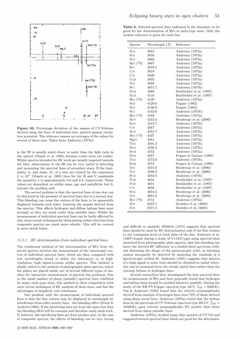
Eclipsing binary stars in open clusters 51
Figure 82. Percentage deviation of the masses of CV Velorumderived using the lines of individual ions, plotted against excita-tion potential. The reference masses are averages of the values forseveral of these ions. Taken from Andersen (1975a).
in the IR is usually much closer to unity than the light ratio inthe optical (Mazeh et al. 1995) because cooler stars are redder.Whilst spectra intended for RV work are usually targeted towardsthe blue, observations in the IR can be very useful in detectingand measuring the spectral lines of secondary stars. If the lumi-nosity, L, and mass, M , of a star are related by the expressionL ∝ Mx (Mazeh et al. 1995) then for the B and V passbandsthe quanitity x is approximately 9.8 and 8.3, respectively. Thesevalues are dependent on stellar mass, age and metallicity but il-lustrate the problem well.
The second problem is that the spectral lines of one star canbe distorted by the presence of spectral lines due to a second star.This blending can cause the centres of the lines to be apparentlydisplaced towards each other, lowering the masses derived fromthe spectra. This affects hydrogen and diffuse helium lines moststrongly as they are much wider than metallic lines. Whilst themeasurement of individual spectral lines can be badly affected bythis, more recent techniques for determining radial velocities fromcomposite spectra are much more reliable. This will be coveredin more detail below.
11.3.1 RV determination from individual spectral lines
The traditional method of the determination of RVs from ob-served spectra involves the measurement of the wavelength cen-tres of individual spectral lines, which are then compared withrest wavelengths found in either the laboratory or in high-resolution, high signal-to-noise stellar spectra. This method isideally suited to the analysis of photographic plate spectra, wherethe plates are placed inside one of several different types of ma-chine for interactive measurement of spectral line positions. Dueto the small number of sharp (metallic) spectral lines exhibitedby many early-type stars, this method is often competitive withmore recent techniques of RV analysis of these stars, and has theadvantages of simplicity and robustness.
One problem with the measurement of individual spectrallines is that the line centres may be displaced in wavelength byinterference from other nearby lines – the blending effect (Petrie &Andrews 1966). If the interfering lines are from the same star thenthe blending effect will be constant and therefore easily dealt with.If, however, the interfering lines are from another star, in the caseof composite spectra, the effects of blending can be very strong
Table 6. Selected spectral lines indicated in the literature to begood for the determination of RVs in early-type stars. Only theearliest reference is given for each line.
Species Wavelength (A) Reference
Si ii 3853 Andersen (1975a)Si ii 3856 Andersen (1975a)Si ii 3862 Andersen (1975a)He i (3S) 3867 Andersen (1975a)Fe i 3878.5 Andersen (1975b)C ii 3919 Andersen (1975a)C ii 3920 Andersen (1975a)Ca ii 3933 Andersen (1975a)N ii 3995 Andersen (1975a)Fe i 4071.7 Andersen (1975b)Si iii 4089 Burkholder et al. (1997)Si iii 4116 Burkholder et al. (1997)He i (3S) 4120 Andersen (1975a)Si ii 4128.0 Popper (1982)Si ii 4130.9 Popper (1982)Fe i 4143.6 Andersen (1975b)He i (1S) 4169 Andersen (1975a)Si iv 4212.4 Hensberge et al. (2000)Sr ii 4215.7 Andersen (1975b)C ii 4267 Andersen (1975a)Fe ii 4351.7 Andersen (1975b)He i (1S) 4437 Andersen (1975a)Mg ii 4481 Andersen (1975a)Ti ii 4501.3 Andersen (1975b)Fe ii 4508.3 Andersen (1975b)Si iii 4552 Andersen (1975a)Si iii 4567 Popper & Guinan (1998)Ti ii 4572.0 Andersen (1975b)Si iii 4574 Popper & Guinan (1998)O ii 4591.0 Hensberge et al. (2000)O ii 4596.2 Hensberge et al. (2000)Fe ii 4583.8 Andersen (1975b)N iii 4634 Burkholder et al. (1997)N iii 4641 Burkholder et al. (1997)C ii 4650 Burkholder et al. (1997)Si iv 4654.3 Hensberge et al. (2000)O ii 4661.6 Hensberge et al. (2000)He i (3S) 4713 Andersen (1975a)Si ii 6347.1 Zwahlen et al. (2004)Si ii 6371.4 Zwahlen et al. (2004)
and difficult to quantify. Hilditch (1973) suggests that spectrallines should be used for RV determination only if the flux returnsto the continuum level on both sides of the line. Andersen et al.(1987) found, during a study of V1143 Cygni using spectral linesmeasured from photographic plate spectra, that line blending canlower the derived RV difference in a double-lined spectrum with-out distorting the shape of the spectroscopic orbit, so blendingcannot necessarily be detected by analysing the residuals of aspectroscopic orbital fit. Andersen (1991) suggests that spectraof a high signal to noise ratio should be obtained so radial veloci-ties can be measured from the (weak) metal lines rather than the(strong) helium or hydrogen lines.
Several researchers have investigated the best spectral linesfor measurement of RVs and have generally found that hydrogenand helium lines should be avoided wherever possible. During thestudy of the EB PV Puppis (spectral type A8 V, Teff = 6920 K),Vaz & Andersen (1984) found that the velocity semiamplitudesderived from analysis of hydrogen lines were 72% of those derivedusing sharp metal lines. Andersen (1975a) noted that the heliumlines in the spectrum of CV Velorum (spectral type B2.5 V, Teff =18300 K), gave velocity semiamplitudes 8% smaller than thosederived from sharp metallic lines.
Andersen (1975a) studied many blue spectra of CV Vel andsuggested several spectral lines which are good for the determina-
c© 0000 RAS, MNRAS 000, 000–000
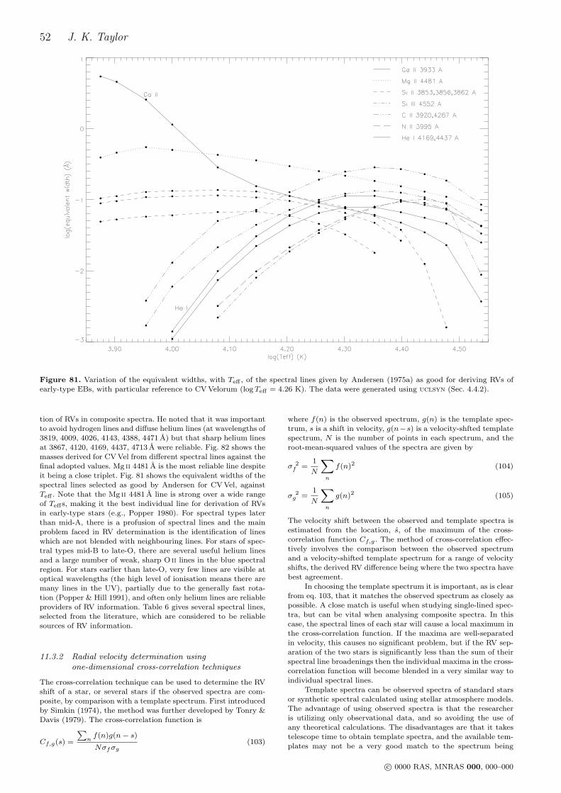
52 J. K. Taylor
Figure 81. Variation of the equivalent widths, with Teff , of the spectral lines given by Andersen (1975a) as good for deriving RVs ofearly-type EBs, with particular reference to CV Velorum (logTeff = 4.26 K). The data were generated using uclsyn (Sec. 4.4.2).
tion of RVs in composite spectra. He noted that it was importantto avoid hydrogen lines and diffuse helium lines (at wavelengths of3819, 4009, 4026, 4143, 4388, 4471 A) but that sharp helium linesat 3867, 4120, 4169, 4437, 4713 A were reliable. Fig. 82 shows themasses derived for CV Vel from different spectral lines against thefinal adopted values. Mg ii 4481 A is the most reliable line despiteit being a close triplet. Fig. 81 shows the equivalent widths of thespectral lines selected as good by Andersen for CV Vel, againstTeff . Note that the Mg ii 4481 A line is strong over a wide rangeof Teffs, making it the best individual line for derivation of RVsin early-type stars (e.g., Popper 1980). For spectral types laterthan mid-A, there is a profusion of spectral lines and the mainproblem faced in RV determination is the identification of lineswhich are not blended with neighbouring lines. For stars of spec-tral types mid-B to late-O, there are several useful helium linesand a large number of weak, sharp O ii lines in the blue spectralregion. For stars earlier than late-O, very few lines are visible atoptical wavelengths (the high level of ionisation means there aremany lines in the UV), partially due to the generally fast rota-tion (Popper & Hill 1991), and often only helium lines are reliableproviders of RV information. Table 6 gives several spectral lines,selected from the literature, which are considered to be reliablesources of RV information.
11.3.2 Radial velocity determination usingone-dimensional cross-correlation techniques
The cross-correlation technique can be used to determine the RVshift of a star, or several stars if the observed spectra are com-posite, by comparison with a template spectrum. First introducedby Simkin (1974), the method was further developed by Tonry &Davis (1979). The cross-correlation function is
Cf,g(s) =
∑nf(n)g(n− s)
Nσfσg(103)
where f(n) is the observed spectrum, g(n) is the template spec-trum, s is a shift in velocity, g(n−s) is a velocity-shfted templatespectrum, N is the number of points in each spectrum, and theroot-mean-squared values of the spectra are given by
σ 2f =
1
N
∑n
f(n)2 (104)
σ 2g =
1
N
∑n
g(n)2 (105)
The velocity shift between the observed and template spectra isestimated from the location, s, of the maximum of the cross-correlation function Cf,g . The method of cross-correlation effec-tively involves the comparison between the observed spectrumand a velocity-shifted template spectrum for a range of velocityshifts, the derived RV difference being where the two spectra havebest agreement.
In choosing the template spectrum it is important, as is clearfrom eq. 103, that it matches the observed spectrum as closely aspossible. A close match is useful when studying single-lined spec-tra, but can be vital when analysing composite spectra. In thiscase, the spectral lines of each star will cause a local maximum inthe cross-correlation function. If the maxima are well-separatedin velocity, this causes no significant problem, but if the RV sep-aration of the two stars is significantly less than the sum of theirspectral line broadenings then the individual maxima in the cross-correlation function will become blended in a very similar way toindividual spectral lines.
Template spectra can be observed spectra of standard starsor synthetic spectral calculated using stellar atmosphere models.The advantage of using observed spectra is that the researcheris utilizing only observational data, and so avoiding the use ofany theoretical calculations. The disadvantages are that it takestelescope time to obtain template spectra, and the available tem-plates may not be a very good match to the spectrum being
c© 0000 RAS, MNRAS 000, 000–000
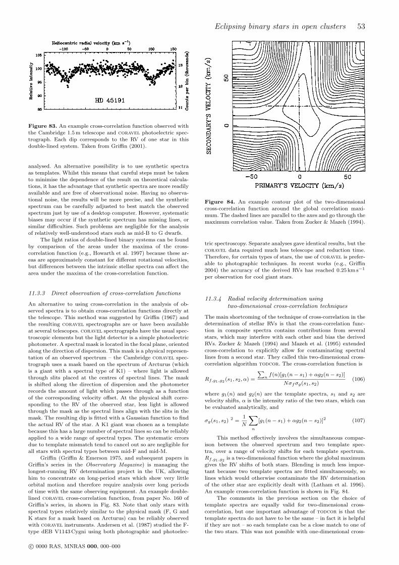
Eclipsing binary stars in open clusters 53
Figure 83. An example cross-correlation function observed withthe Cambridge 1.5 m telescope and coravel photoelectric spec-trograph. Each dip corresponds to the RV of one star in thisdouble-lined system. Taken from Griffin (2001).
analysed. An alternative possibility is to use synthetic spectraas templates. Whilst this means that careful steps must be takento minimise the dependence of the result on theoretical calcula-tions, it has the advantage that synthetic spectra are more readilyavailable and are free of observational noise. Having no observa-tional noise, the results will be more precise, and the syntheticspectrum can be carefully adjusted to best match the observedspectrum just by use of a desktop computer. However, systematicbiases may occur if the synthetic spectrum has missing lines, orsimilar difficulties. Such problems are negligible for the analysisof relatively well-understood stars such as mid-B to G dwarfs.
The light ratios of double-lined binary systems can be foundby comparison of the areas under the maxima of the cross-correlation function (e.g., Howarth et al. 1997) because these ar-eas are approximately constant for different rotational velocities,but differences between the intrinsic stellar spectra can affect thearea under the maxima of the cross-correlation function.
11.3.3 Direct observation of cross-correlation functions
An alternative to using cross-correlation in the analysis of ob-served spectra is to obtain cross-correlation functions directly atthe telescope. This method was suggested by Griffin (1967) andthe resulting coravel spectrographs are or have been availableat several telescopes. coravel spectrographs have the usual spec-troscopic elements but the light detector is a simple photoelectricphotometer. A spectral mask is located in the focal plane, orientedalong the direction of dispersion. This mask is a physical represen-tation of an observed spectrum – the Cambridge coravel spec-trograph uses a mask based on the spectrum of Arcturus (whichis a giant with a spectral type of K1) – where light is allowedthrough slits placed at the centres of spectral lines. The maskis shifted along the direction of dispersion and the photometerrecords the amount of light which passes through as a functionof the corresponding velocity offset. At the physical shift corre-sponding to the RV of the observed star, less light is allowedthrough the mask as the spectral lines align with the slits in themask. The resulting dip is fitted with a Gaussian function to findthe actual RV of the star. A K1 giant was chosen as a templatebecause this has a large number of spectral lines so can be reliablyapplied to a wide range of spectral types. The systematic errorsdue to template mismatch tend to cancel out so are negligible forall stars with spectral types between mid-F and mid-M.
Griffin (Griffin & Emerson 1975, and subsequent papers inGriffin’s series in the Observatory Magazine) is managing thelongest-running RV determination project in the UK, allowinghim to concentrate on long-period stars which show very littleorbital motion and therefore require analysis over long periodsof time with the same observing equipment. An example double-lined coravel cross-correlation function, from paper No. 160 ofGriffin’s series, in shown in Fig. 83. Note that only stars withspectral types relatively similar to the physical mask (F, G andK stars for a mask based on Arcturus) can be reliably observedwith coravel instruments. Andersen et al. (1987) studied the F-type dEB V1143 Cygni using both photographic and photoelec-
Figure 84. An example contour plot of the two-dimensionalcross-correlation function around the global correlation maxi-mum. The dashed lines are parallel to the axes and go through themaximum correlation value. Taken from Zucker & Mazeh (1994).
tric spectroscopy. Separate analyses gave identical results, but thecoravel data required much less telescope and reduction time.Therefore, for certain types of stars, the use of coravel is prefer-able to photographic techniques. In recent works (e.g., Griffin2004) the accuracy of the derived RVs has reached 0.25 km s−1
per observation for cool giant stars.
11.3.4 Radial velocity determination usingtwo-dimensional cross-correlation techniques
The main shortcoming of the technique of cross-correlation in thedetermination of stellar RVs is that the cross-correlation func-tion in composite spectra contains contributions from severalstars, which may interfere with each other and bias the derivedRVs. Zucker & Mazeh (1994) and Mazeh et al. (1995) extendedcross-correlation to explicitly allow for contaminating spectrallines from a second star. They called this two-dimensional cross-correlation algorithm todcor. The cross-correlation function is
Rf,g1,g2 (s1, s2, α) =
∑nf(n)[g1(n− s1) + αg2(n− s2)]
Nσfσg(s1, s2)(106)
where g1(n) and g2(n) are the template spectra, s1 and s2 arevelocity shifts, α is the intensity ratio of the two stars, which canbe evaluated analytically, and
σg(s1, s2) 2 =1
N
∑n
[g1(n− s1) + αg2(n− s2)]2 (107)
This method effectively involves the simultaneous compar-ison between the observed spectrum and two template spec-tra, over a range of velocity shifts for each template spectrum.Rf,g1,g2 is a two-dimensional function where the global maximumgives the RV shifts of both stars. Blending is much less impor-tant because two template spectra are fitted simultaneously, solines which would otherwise contaminate the RV determinationof the other star are explicitly dealt with (Latham et al. 1996).An example cross-correlation function is shown in Fig. 84.
The comments in the previous section on the choice oftemplate spectra are equally valid for two-dimensional cross-correlation, but one important advantage of todcor is that thetemplate spectra do not have to be the same – in fact it is helpfulif they are not – so each template can be a close match to one ofthe two stars. This was not possible with one-dimensional cross-
c© 0000 RAS, MNRAS 000, 000–000
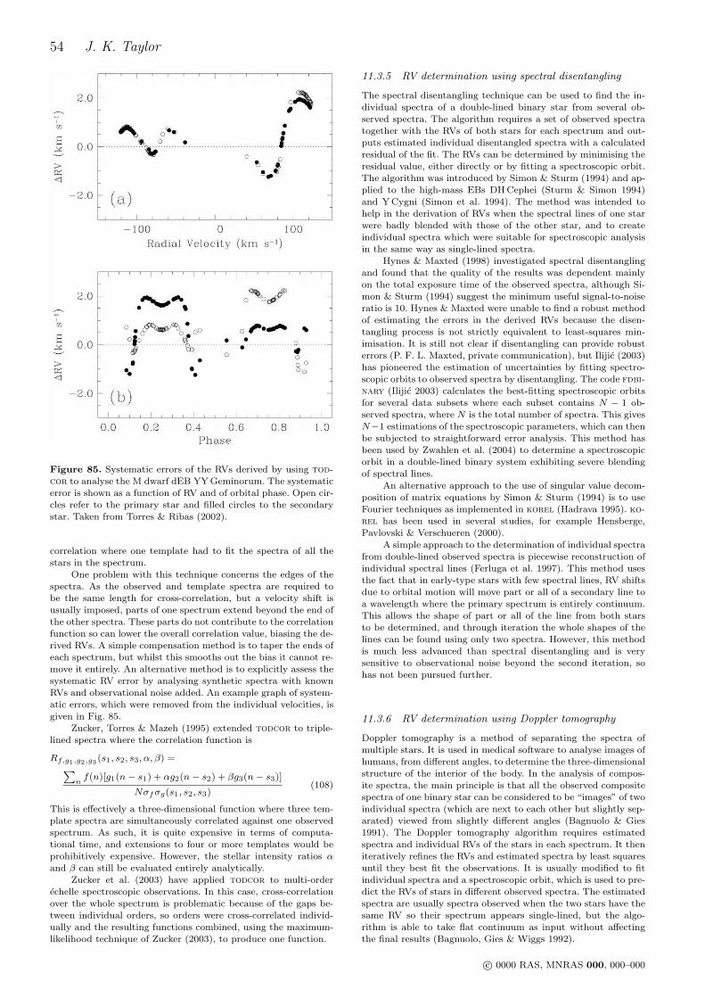
54 J. K. Taylor
Figure 85. Systematic errors of the RVs derived by using tod-cor to analyse the M dwarf dEB YY Geminorum. The systematicerror is shown as a function of RV and of orbital phase. Open cir-cles refer to the primary star and filled circles to the secondarystar. Taken from Torres & Ribas (2002).
correlation where one template had to fit the spectra of all thestars in the spectrum.
One problem with this technique concerns the edges of thespectra. As the observed and template spectra are required tobe the same length for cross-correlation, but a velocity shift isusually imposed, parts of one spectrum extend beyond the end ofthe other spectra. These parts do not contribute to the correlationfunction so can lower the overall correlation value, biasing the de-rived RVs. A simple compensation method is to taper the ends ofeach spectrum, but whilst this smooths out the bias it cannot re-move it entirely. An alternative method is to explicitly assess thesystematic RV error by analysing synthetic spectra with knownRVs and observational noise added. An example graph of system-atic errors, which were removed from the individual velocities, isgiven in Fig. 85.
Zucker, Torres & Mazeh (1995) extended todcor to triple-lined spectra where the correlation function is
Rf,g1,g2,g3 (s1, s2, s3, α, β) =∑
nf(n)[g1(n− s1) + αg2(n− s2) + βg3(n− s3)]
Nσfσg(s1, s2, s3)(108)
This is effectively a three-dimensional function where three tem-plate spectra are simultaneously correlated against one observedspectrum. As such, it is quite expensive in terms of computa-tional time, and extensions to four or more templates would beprohibitively expensive. However, the stellar intensity ratios αand β can still be evaluated entirely analytically.
Zucker et al. (2003) have applied todcor to multi-orderechelle spectroscopic observations. In this case, cross-correlationover the whole spectrum is problematic because of the gaps be-tween individual orders, so orders were cross-correlated individ-ually and the resulting functions combined, using the maximum-likelihood technique of Zucker (2003), to produce one function.
11.3.5 RV determination using spectral disentangling
The spectral disentangling technique can be used to find the in-dividual spectra of a double-lined binary star from several ob-served spectra. The algorithm requires a set of observed spectratogether with the RVs of both stars for each spectrum and out-puts estimated individual disentangled spectra with a calculatedresidual of the fit. The RVs can be determined by minimising theresidual value, either directly or by fitting a spectroscopic orbit.The algorithm was introduced by Simon & Sturm (1994) and ap-plied to the high-mass EBs DH Cephei (Sturm & Simon 1994)and Y Cygni (Simon et al. 1994). The method was intended tohelp in the derivation of RVs when the spectral lines of one starwere badly blended with those of the other star, and to createindividual spectra which were suitable for spectroscopic analysisin the same way as single-lined spectra.
Hynes & Maxted (1998) investigated spectral disentanglingand found that the quality of the results was dependent mainlyon the total exposure time of the observed spectra, although Si-mon & Sturm (1994) suggest the minimum useful signal-to-noiseratio is 10. Hynes & Maxted were unable to find a robust methodof estimating the errors in the derived RVs because the disen-tangling process is not strictly equivalent to least-squares min-imisation. It is still not clear if disentangling can provide robusterrors (P. F. L. Maxted, private communication), but Ilijic (2003)has pioneered the estimation of uncertainties by fitting spectro-scopic orbits to observed spectra by disentangling. The code fdbi-nary (Ilijic 2003) calculates the best-fitting spectroscopic orbitsfor several data subsets where each subset contains N − 1 ob-served spectra, where N is the total number of spectra. This givesN−1 estimations of the spectroscopic parameters, which can thenbe subjected to straightforward error analysis. This method hasbeen used by Zwahlen et al. (2004) to determine a spectroscopicorbit in a double-lined binary system exhibiting severe blendingof spectral lines.
An alternative approach to the use of singular value decom-position of matrix equations by Simon & Sturm (1994) is to useFourier techniques as implemented in korel (Hadrava 1995). ko-rel has been used in several studies, for example Hensberge,Pavlovski & Verschueren (2000).
A simple approach to the determination of individual spectrafrom double-lined observed spectra is piecewise reconstruction ofindividual spectral lines (Ferluga et al. 1997). This method usesthe fact that in early-type stars with few spectral lines, RV shiftsdue to orbital motion will move part or all of a secondary line toa wavelength where the primary spectrum is entirely continuum.This allows the shape of part or all of the line from both starsto be determined, and through iteration the whole shapes of thelines can be found using only two spectra. However, this methodis much less advanced than spectral disentangling and is verysensitive to observational noise beyond the second iteration, sohas not been pursued further.
11.3.6 RV determination using Doppler tomography
Doppler tomography is a method of separating the spectra ofmultiple stars. It is used in medical software to analyse images ofhumans, from different angles, to determine the three-dimensionalstructure of the interior of the body. In the analysis of compos-ite spectra, the main principle is that all the observed compositespectra of one binary star can be considered to be “images” of twoindividual spectra (which are next to each other but slightly sep-arated) viewed from slightly different angles (Bagnuolo & Gies1991). The Doppler tomography algorithm requires estimatedspectra and individual RVs of the stars in each spectrum. It theniteratively refines the RVs and estimated spectra by least squaresuntil they best fit the observations. It is usually modified to fitindividual spectra and a spectroscopic orbit, which is used to pre-dict the RVs of stars in different observed spectra. The estimatedspectra are usually spectra observed when the two stars have thesame RV so their spectrum appears single-lined, but the algo-rithm is able to take flat continuum as input without affectingthe final results (Bagnuolo, Gies & Wiggs 1992).
c© 0000 RAS, MNRAS 000, 000–000
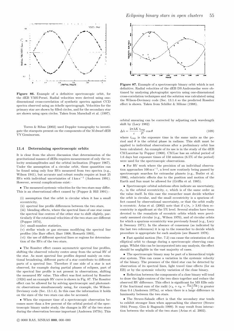
Eclipsing binary stars in open clusters 55
Figure 86. Example of a definitive spectroscopic orbit, forthe dEB V505 Persei. Radial velocities were derived using one-dimensional cross-correlation of synthetic spectra against CCDspectra observed using an echelle spectrograph. Velocities for theprimary star are shown by filled circles, and for the secondary starare shown using open circles. Taken from Marschall et al. (1997).
Torres & Ribas (2002) used Doppler tomography to investi-gate the starspots present on the components of the M dwarf dEBYY Geminorum.
11.4 Determining spectroscopic orbits
It is clear from the above discussion that determination of thegravitational masses of dEBs requires measurement of only the ve-locity semiamplitudes and the orbital inclination (Popper 1967).Under the assumption of a circular orbit, these quantities canbe found using only four RVs measured from two spectra (e.g.,Wilson 1941), but accurate and robust results require at least 25RVs with individual uncertainties of 1 km s−1 (Andersen 1991).However, several complications exist:–
• The measured systemic velocities for the two stars may differ.This is an observational effect caused by (Popper & Hill 1991):–
(i) assumption that the orbit is circular when it has a smalleccentricity,
(ii) spectral line profile differences between the two stars,
(iii) blending effects, where the spectral lines of one star causethe spectral line centres of the other star to shift slightly, par-ticularly if the rotational velocities of the two stars are different(Popper 1974),
(iv) small-number statistics,
(v) stellar winds or gas streams modifying the spectral lineprofiles (the Barr effect; Barr 1908; Howarth 1993),
(vi) the use of different spectral lines or regions for determina-tion of the RVs of the two stars.
• The Rossiter effect causes asymmetric spectral line profiles,shifting the observed velocity centre away from the actual RV ofthe star. As most spectral line profiles depend mainly on rota-tional broadening, different parts of a star contribute to differentparts of a spectral line. Therefore if one side of a star is notobserved, for example during partial phases of eclipses, part ofthe spectral line profile is not present in observations, shiftingthe measured RV value. This effect was first noticed by Rossiter(1924) and an example RV curve is shown in Fig. 87. The Rossitereffect can be allowed for by solving spectroscopic and photomet-ric observations simultaneously using, for example, the Wilson-Devinney code (Sec. 13.1.4). In this case the information it holdson the sizes of the two stars can also be accessed.
• When the exposure time of a spectroscopic observation be-comes more than a few percent of the orbital period of the spec-troscopic binary under study, the changes in RV of the two starsduring the observation become important (Andersen 1975b). This
Figure 87. Example of a spectroscopic binary orbit which is notdefinitive. Radial velocities of the dEB DS Andromedae were ob-tianed by analysing photographic spectra using one-dimensionalcross-correlation techniques and the solution was calculated usingthe Wilson-Devinney code (Sec. 13.1.4 so the predicted Rossitereffect is shown. Taken from Schiller & Milone (1988).
orbital smearing can be corrected by adjusting each wavelengthshift by (Lacy 1982)
∆λ =2πλK
c
texp
Pcos θ (109)
where texp is the exposure time in the same units as the pe-riod and θ is the orbital phase in radians. This shift must beapplied to individual observations after a preliminary orbit hasbeen calculated. An example of its use is in the study of the dEBCM Lacertae by Popper (1968). CM Lac has an orbital period of1.6 days but exposure times of 150 minutes (6.5% of the period)were used for the spectroscopic observations.
• For RV work where the precision of an individual observa-tion approaches 100 m s−1, a level now routinely being passed byspectroscopic searches for extrasolar planets (e.g., Butler et al.1996), relativistic effects due to the position and motion of theEarth and Sun must be allowed for (Griffin et al. 1985).
• Spectroscopic orbital solutions often indicate an uncertainty,σe, in the orbital eccentricity, e, which is of the same order asthe value itself. In this case the researcher must decide whetherthe orbit is circular, and the small eccentricity is a spurious ef-fect caused by observational uncertainty, or that the orbit reallyis eccentric. Arias et al. (2002) note that if e/σe > 3.83 then ec-centricity is significant at the 5% level. Several studies have beendevoted to the reanalysis of eccentric orbits which were previ-ously assumed circular (e.g., Wilson 1970), and of circular orbitsfor which a spurious eccentricity was previously found (e.g., Lucy& Sweeney 1971). In the absence of consensus (as indicated bythe last two references) it is up to the researcher to decide whichprocedure is appropriate for each analysis (see Bassett 1978).
• Fast apsidal motion (Sec. 7.2) can cause the orientation of anelliptical orbit to change during a spectroscopic observing cam-paign. Whilst this can be incorporated into any analysis, the effectshould be negligible in the vast majority of cases.
• The spectroscopic binary may be part of a hierarchical triplestar system. This can cause a variation in the systemic velocityof the binary. The presence of the third star can be detected byobservation of its spectral lines, light travel time effects (for anEB) or by the systemic velocity variation of the close binary.
• Reflection between the components of a close binary will tendto draw the light-centres of the two discs together and reduce theobserved RV difference. This effect is significant for MS EBs onlyif the fractional sum of the radii (rA + rB = RA+RB
a) is greater
than 0.4 (Andersen 1975a), or when there is a large difference inluminosity between the two stars.
• The Struve-Sahade effect is that the secondary star tendsto exhibit stronger lines when approaching the observer (Struve1944; Penny, Gies & Bagnuolo 1999). It may result from interac-tion between the winds of the two stars (Arias et al. 2002).
c© 0000 RAS, MNRAS 000, 000–000
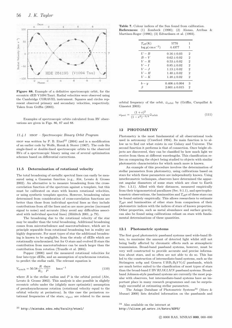
56 J. K. Taylor
Figure 88. Example of a definitive spectroscopic orbit, for theeccentric dEB V1094 Tauri. Radial velocities were observed usingthe Cambridge CORAVEL instrument. Squares and circles rep-resent observed primary and secondary velocities, respectively.Taken from Griffin (2003).
Examples of spectroscopic orbits calculated from RV obser-vations are given in Figs. 86, 87 and 88.
11.4.1 sbop – Spectroscopic Binary Orbit Program
sbop was written by P. B. Etzel33 (2004) and is a modificationof an earlier code by Wolfe, Horak & Storer (1967). The code fitssingle-lined or double-lined spectroscopic orbits to the observedRVs of a spectroscopic binary using one of several optimisationschemes based on differential corrections.
11.5 Determination of rotational velocity
The total broadening of metallic spectral lines can easily be mea-sured using a Gaussian function (e.g., Abt, Levato & Grosso2002). An alternative is to measure broadening from the cross-correlation function of the spectrum against a template, but thismust be calibrated on stars with known rotational velocities,or using synthetic template spectra. However, broadening valuesdetermined from consideration of cross-correlation functions arebetter than those from individual spectral lines as they includecontributions from all the lines and so are more precise (increasedsignal to noise) and accurate (they avoid any difficulties associ-ated with individual spectral lines) (Hilditch 2001, p. 79).
The broadening due to the rotational velocity of the starmay be smaller than the total broadening. Additional broadeningcomes from microturbulence and macroturbulence, which are inprinciple separable from rotational broadening but in reality arehighly degenerate. For most types of star the additional broaden-ing is known to be negligible, from the study of dEBs which arerotationally synchronized, but for O stars and evolved B stars thecontribution from macroturbulence can be much larger than thecontribution from rotation (Trundle et al. 2004).
Popper (2000) used the measured rotational velocities forfour late-type dEBs, and an assumption of synchronous rotation,to predict the stellar radii. The relevant equation is
Vsynch = 50.58R
R¯days
Pkm s−1 (110)
where R is the stellar radius and P is the orbital period (Abt,Levato & Grosso 2002). This analysis is also possible in slightlyeccentric orbits under the (slightly more optimistic) assumptionof pseudosynchronous rotation (rotational velocity equal to theorbital velocity at periastron). In this case the periastron ro-tational frequencies of the stars, ωperi are related to the mean
33 http://mintaka.sdsu.edu/faculty/etzel/
Table 7. Colour indices of the Sun found from calibration.References: (1) Zombeck (1990); (2) Alonso, Arribas &Martınez-Roger (1996); (3) Edvardssen et al. (1993).
Teff(K) 5770 1log g( cm s−2) 4.4377 1
U −B 0.16± 0.03 2B − V 0.62± 0.02 2V −R 0.53± 0.02 2V − I 0.85± 0.02 2V − J 1.13± 0.02 2V −H 1.40± 0.02 2V −K 1.48± 0.02 2
b− y 0.406± 0.004 3β 2.601± 0.015 2
orbital frequency of the orbit, ωorbit by (Griffin, Carquillat &Ginestet 2003):
ωperi =(1 + e)2
(1− e2)−3/2ωorbit (111)
12 PHOTOMETRY
Photometry is the most fundamental of all observational toolsused in astronomy (Crawford 1994). Its main function is to al-low us to find out what exists in our Galaxy and Universe. Thesecond function it performs is that of connection. Once bright ob-jects are discovered, they can be classified by how much light wereceive from them at different wavelengths. This classification re-lies on comparing the object being studied to objects with similarphotometric characteristics for which much more is known.
An example of this procedure involves the determination ofstellar parameters from photometry, using calibrations based onstars for which these parameters are independently known. Usinginterferometric techniques, observers have determined the appar-ent angular diameters of some stars which are close to Earth(Sec. 1.3.1). Allied with their distances, measured empiricallyfrom their trigonometrical parallaxes (Sec. 9.1.1), and spectropho-tometric observations, the luminosities and Teffs of these stars canbe found entirely empirically. This allows researchers to estimateTeffs and luminosities of other stars from comparison of theirphotometric indices with the indices of stars of known properties.Other properties, such as metal abundance and surface gravity,can also be found using calibrations reliant on stars with funda-mental determinations of these quantities.
12.1 Photometric systems
The first good photometric passband systems used wide-band fil-ters, to maximise the amount of detected light whilst still notbeing badly affected by chromatic effects such as atmospherictransmission. Broad-band passband systems, however, must bevery well constructed to provide accurate and precise informa-tion about stars, and so often are not able to do so. This hasled to the construction of intermediate-band systems, such as theStromgren uvby and Geneva UBB1B2V V1G passbands, whichare much better suited to the classification of most types of starsthan the broad-band UBV RIJKLMN passband systems. Broad-band Johnson-style passband systems are currently the most pop-ular with observers, but intermediate-band systems have an im-portant place in many research programmes and can be surpris-ingly successful at estimating stellar parameters.
The Asiago Database of Photometric Systems34 (Moro &Munari 2000) lists detailed information on the passbands and
34 Also available on the internet athttp://ulisse.pd.astro.it/Astro/ADPS/
c© 0000 RAS, MNRAS 000, 000–000
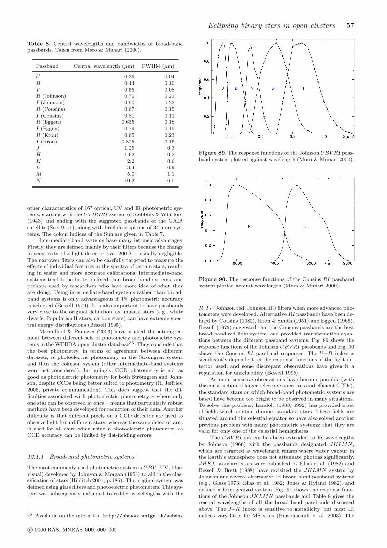
Eclipsing binary stars in open clusters 57
Table 8. Central wavelengths and bandwidths of broad-bandpassbands. Taken from Moro & Munari (2000).
Passband Central wavelength (µm) FWHM (µm)
U 0.36 0.04B 0.44 0.10V 0.55 0.08R (Johnson) 0.70 0.21I (Johnson) 0.90 0.22R (Cousins) 0.67 0.15I (Cousins) 0.81 0.11R (Eggen) 0.635 0.18I (Eggen) 0.79 0.15R (Kron) 0.65 0.23I (Kron) 0.825 0.15J 1.25 0.3H 1.62 0.2K 2.2 0.6L 3.4 0.9M 5.0 1.1N 10.2 6.0
other characteristics of 167 optical, UV and IR photometric sys-tems, starting with the UV BGRI system of Stebbins & Whitford(1943) and ending with the suggested passbands of the GAIAsatellite (Sec. 9.1.1), along with brief descriptions of 34 more sys-tems. The colour indices of the Sun are given in Table 7.
Intermediate band systems have many intrinsic advantages.Firstly, they are defined mainly by their filters because the changein sensitivity of a light detector over 200 A is usually negligible.The narrower filters can also be carefully targeted to measure theeffects of individual features in the spectra of certain stars, result-ing in easier and more accurate calibrations. Intermediate-bandsystems tend to be better defined than broad-band systems, andperhaps used by researchers who have more idea of what theyare doing. Using intermediate-band systems rather than broad-band systems is only advantageous if 1% photometric accuracyis achieved (Bessell 1979). It is also important to have passbandsvery close to the original definition, as unusual stars (e.g., whitedwarfs, Population II stars, carbon stars) can have extreme spec-tral energy distributions (Bessell 1995).
Mermilliod & Paunzen (2003) have studied the interagree-ment between different sets of photometry and photometric sys-tems in the WEBDA open cluster database35. They conclude thatthe best photometry, in terms of agreement between differentdatasets, is photoelectric photometry in the Stromgren systemand then the Johnson system (other intermediate-band systemswere not considered). Intriguingly, CCD photometry is not asgood as photoelectric photometry for both Stromgren and John-son, despite CCDs being better suited to photometry (R. Jeffries,2005, private communication). This does suggest that the dif-ficulties associated with photoelectric photometry – where onlyone star can be observed at once – means that particularly robustmethods have been developed for reduction of their data. Anotherdifficulty is that different pixels on a CCD detector are used toobserve light from different stars, whereas the same detector areais used for all stars when using a photoelectric photometer, soCCD accuracy can be limited by flat-fielding errors.
12.1.1 Broad-band photometric systems
The most commonly used photometric system is UBV (UV, blue,visual) developed by Johnson & Morgan (1953) to aid in the clas-sification of stars (Hilditch 2001, p. 186). The original system wasdefined using glass filters and photoelectric photometers. This sys-tem was subsequently extended to redder wavelengths with the
35 Available on the internet at http://obswww.unige.ch/webda/
Figure 89. The response functions of the Johnson UBV RI pass-band system plotted against wavelength (Moro & Munari 2000).
Figure 90. The response functions of the Cousins RI passbandsystem plotted against wavelength (Moro & Munari 2000).
RJIJ (Johnson red, Johnson IR) filters when more advanced pho-tometers were developed. Alternative RI passbands have been de-fined by Cousins (1980), Kron & Smith (1951) and Eggen (1965).Bessell (1979) suggested that the Cousins passbands are the bestbroad-band red-light system, and provided transformation equa-tions between the different passband systems. Fig. 89 shows theresponse functions of the Johnson UBV RI passbands and Fig. 90shows the Cousins RI passband responses. The U−B index issignificantly dependent on the response functions of the light de-tector used, and some discrepant observations have given it areputation for unreliability (Bessell 1995).
As more sensitive observations have become possible (withthe construction of larger telescope apertures and efficient CCDs),the standard stars on which broad-band photometric systems arebased have become too bright to be observed in many situations.To solve this problem, Landolt (1983, 1992) has provided a setof fields which contain dimmer standard stars. These fields aresituated around the celestial equator so have also solved anotherprevious problem with many photometric systems; that they arevalid for only one of the celestial hemispheres.
The UBV RI system has been extended to IR wavelengthsby Johnson (1966) with the passbands designated JKLMN ,which are targeted at wavelength ranges where water vapour inthe Earth’s atmosphere does not attenuate photons significantly.JHKL standard stars were published by Elias et al. (1982) andBessell & Brett (1988) have revisited the JKLMN system byJohnson and several alternative IR broad-band passband systems(e.g., Glass 1973; Elias et al. 1982; Jones & Hyland 1982), anddefined a homogenized system. Fig. 91 shows the response func-tions of the Johnson JKLMN passbands and Table 8 gives thecentral wavelengths of all the broad-band passbands discussedabove. The J−K index is sensitive to metallicity, but most IRindices vary little for MS stars (Pinsonneault et al. 2003). The
c© 0000 RAS, MNRAS 000, 000–000
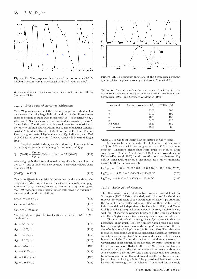
58 J. K. Taylor
Figure 91. The response functions of the Johnson JKLMNpassband system versus wavelength. (Moro & Munari 2000).
K passband is very insensitive to surface gravity and metallicity(Johnson 1966).
12.1.2 Broad-band photometric calibrations
UBV RI photometry is not the best way to get individual stellarparameters, but the large light throughput of the filters causesthem to remain popular with researchers. B−V is sensitive to Teff
whereas U−B is sensitive to Teff and surface gravity (Phelps &Janes 1994). The B passband is also known to be sensitive tometallicity via flux redistribution due to line blanketing (Alonso,Arribas & Martınez-Roger 1996). However, for F, G and K starsV−I is a good metallicity-independent Teff indicator, and R−Iis useful for later-type stars (Alonso, Arribas & Martınez-Roger1996)
The photometric index Q was introduced by Johnson & Mor-gan (1953) to provide a reddening-free estimator of Teff :
Q = (U−B)− EU−B
EB−V(B−V ) = (U−B)− 0.72(B−V ) (112)
where EX−Y is the interstellar reddening effect in the colour in-dex X−Y . The Q index can also be used to deredden colours using(Johnson 1958):
(B−V )0 = 0.332Q (113)
The ratioEU−B
EB−Vis empirically determined and depends on the
properties of the interstellar matter which causes reddening (e.g.,Reimann 1989). Barnes, Evans & Moffett (1978) investigatedUBV RI reddening using interferometrically measured angular di-ameters and found the relations
EU−B = 0.75EB−V (114)
EV−R = 0.75EB−V (115)
ER−I = 0.76EB−V (116)
Moro & Munari give the total extinction in the UBV RIJKLbands to be
AU = 4.4EB−V (117)
AB = 4.1EB−V (118)
AV = 3.1EB−V (119)
AR = 2.3EB−V (120)
AI = 1.5EB−V (121)
AJ = 0.87EB−V (122)
AK = 0.38EB−V (123)
AL = 0.16EB−V (124)
Figure 92. The response functions of the Stromgren passbandsystem plotted against wavelength (Moro & Munari 2000).
Table 9. Central wavelengths and spectral widths for theStromgren-Crawford uvbyβ photometric system. Data taken fromStromgren (1963) and Crawford & Mander (1966).
Passband Central wavelength (A) FWHM (A)
u 3500 300v 4110 190b 4670 180y 5470 220Hβ wide 4861 150Hβ narrow 4861 30
where AV is the total interstellar extinction in the V band.Q is a useful Teff indicator for hot stars, but the value
of Q for MS stars with masses greater than 30 M¯ is almostconstant. Therefore higher-mass stars must be studied usingspectroscopy (Massey & Johnson 1993). Massey, Waterhouse &DeGioia-Eastwood (2000) found theoretical relations between Teff
and Q, using Kurucz model atmospheres, for stars of luminosityclasses I, III and V, respectively:
log TeffI = −0.9894−22.76738Q−33.09637Q2−16.19307Q3(125)
log TeffIII = 5.2618− 3.42004Q− 2.93489Q2 (126)
log TeffV = 4.2622− 0.64525Q− 1.09174Q2 (127)
12.1.3 Stromgren photometry
The Stromgren uvby photometric system was defined byStromgren (1963, 1966), and is designed to be used for the simul-taneous determination of the parameters of early-type stars andthe amount of interstellar reddening affecting their light. The Hβindex was defined independently by Crawford (1958) and Craw-ford & Mander (1966) and complements the uvby passbands verywell. Fig. 92 shows the response functions of the uvbyβ passbandsand Table 9 gives the central wavelengths and spectral widths.
The main drawback of using the uvbyβ system is that thepassbands allow much less light through than broad-band pass-bands; the original uvby passbands had peak transmission efficien-cies of only about 50% (Crawford & Barnes 1970). The advantageis that the passbands are good at measuring particular features inearly-type stellar spectra. The u passband measures flux densitybluewards of the Balmer discontinuity, but does not extend towavelengths short enough to be affected by water vapour in theEarth’s atmosphere (Hilditch 2001, p. 192). The v passband istargeted at a part of the spectrum where iron lines are abundantso is sensitive to metallicity. The b and y passbands are intendedto measure continuum flux and are sufficiently red to not be sub-ject to line blanketing effects. The y passband has a very simi-lar central wavelength to the Johnson V passband and is closely
c© 0000 RAS, MNRAS 000, 000–000
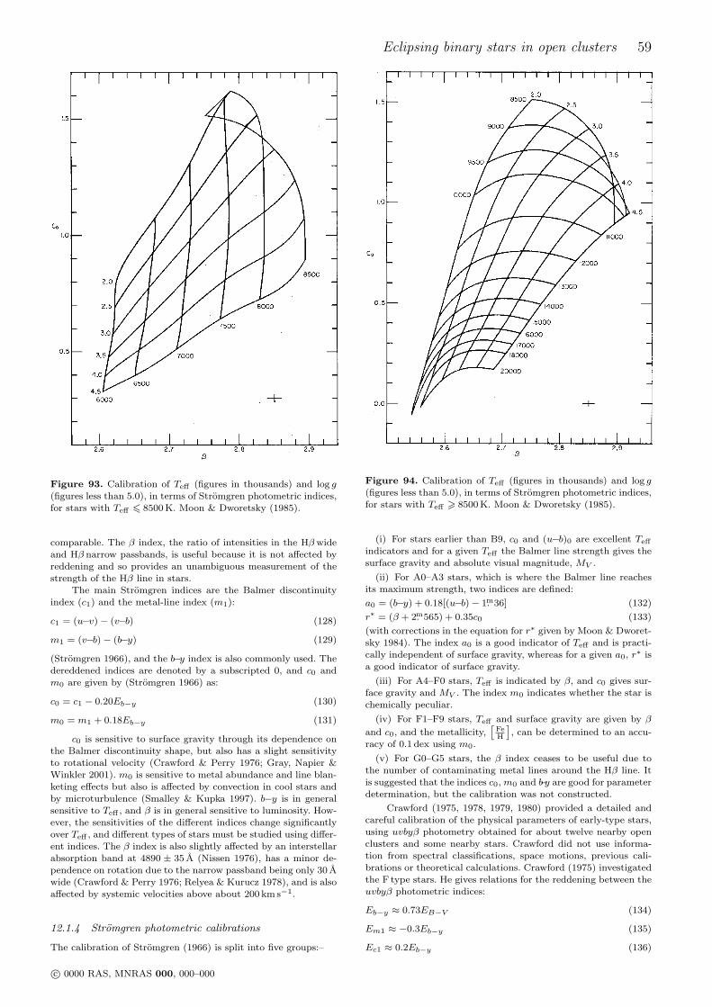
Eclipsing binary stars in open clusters 59
Figure 93. Calibration of Teff (figures in thousands) and log g(figures less than 5.0), in terms of Stromgren photometric indices,for stars with Teff 6 8500 K. Moon & Dworetsky (1985).
comparable. The β index, the ratio of intensities in the Hβwideand Hβ narrow passbands, is useful because it is not affected byreddening and so provides an unambiguous measurement of thestrength of the Hβ line in stars.
The main Stromgren indices are the Balmer discontinuityindex (c1) and the metal-line index (m1):
c1 = (u−v)− (v−b) (128)
m1 = (v−b)− (b−y) (129)
(Stromgren 1966), and the b−y index is also commonly used. Thedereddened indices are denoted by a subscripted 0, and c0 andm0 are given by (Stromgren 1966) as:
c0 = c1 − 0.20Eb−y (130)
m0 = m1 + 0.18Eb−y (131)
c0 is sensitive to surface gravity through its dependence onthe Balmer discontinuity shape, but also has a slight sensitivityto rotational velocity (Crawford & Perry 1976; Gray, Napier &Winkler 2001). m0 is sensitive to metal abundance and line blan-keting effects but also is affected by convection in cool stars andby microturbulence (Smalley & Kupka 1997). b−y is in generalsensitive to Teff , and β is in general sensitive to luminosity. How-ever, the sensitivities of the different indices change significantlyover Teff , and different types of stars must be studied using differ-ent indices. The β index is also slightly affected by an interstellarabsorption band at 4890 ± 35 A (Nissen 1976), has a minor de-pendence on rotation due to the narrow passband being only 30 Awide (Crawford & Perry 1976; Relyea & Kurucz 1978), and is alsoaffected by systemic velocities above about 200 km s−1.
12.1.4 Stromgren photometric calibrations
The calibration of Stromgren (1966) is split into five groups:–
Figure 94. Calibration of Teff (figures in thousands) and log g(figures less than 5.0), in terms of Stromgren photometric indices,for stars with Teff > 8500 K. Moon & Dworetsky (1985).
(i) For stars earlier than B9, c0 and (u−b)0 are excellent Teff
indicators and for a given Teff the Balmer line strength gives thesurface gravity and absolute visual magnitude, MV .
(ii) For A0–A3 stars, which is where the Balmer line reachesits maximum strength, two indices are defined:
a0 = (b−y) + 0.18[(u−b)− 1.m36] (132)
r∗ = (β + 2.m565) + 0.35c0 (133)
(with corrections in the equation for r∗ given by Moon & Dworet-sky 1984). The index a0 is a good indicator of Teff and is practi-cally independent of surface gravity, whereas for a given a0, r∗ isa good indicator of surface gravity.
(iii) For A4–F0 stars, Teff is indicated by β, and c0 gives sur-face gravity and MV . The index m0 indicates whether the star ischemically peculiar.
(iv) For F1–F9 stars, Teff and surface gravity are given by β
and c0, and the metallicity,[
FeH
], can be determined to an accu-
racy of 0.1 dex using m0.
(v) For G0–G5 stars, the β index ceases to be useful due tothe number of contaminating metal lines around the Hβ line. Itis suggested that the indices c0, m0 and b−y are good for parameterdetermination, but the calibration was not constructed.
Crawford (1975, 1978, 1979, 1980) provided a detailed andcareful calibration of the physical parameters of early-type stars,using uvbyβ photometry obtained for about twelve nearby openclusters and some nearby stars. Crawford did not use informa-tion from spectral classifications, space motions, previous cali-brations or theoretical calculations. Crawford (1975) investigatedthe F type stars. He gives relations for the reddening between theuvbyβ photometric indices:
Eb−y ≈ 0.73EB−V (134)
Em1 ≈ −0.3Eb−y (135)
Ec1 ≈ 0.2Eb−y (136)
c© 0000 RAS, MNRAS 000, 000–000
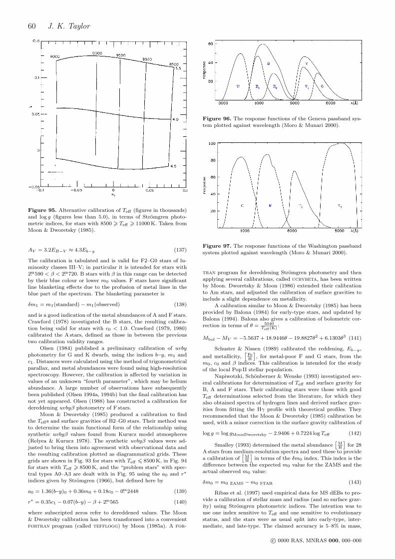
60 J. K. Taylor
Figure 95. Alternative calibration of Teff (figures in thousands)and log g (figures less than 5.0), in terms of Stromgren photo-metric indices, for stars with 8500 > Teff > 11000 K. Taken fromMoon & Dworetsky (1985).
AV = 3.2EB−V ≈ 4.3Eb−y (137)
The calibration is tabulated and is valid for F2–G0 stars of lu-minosity classes III–V; in particular it is intended for stars with2.m590 < β < 2.m720. B stars with β in this range can be detectedby their blue colour or lower m0 values. F stars have significantline blanketing effects due to the profusion of metal lines in theblue part of the spectrum. The blanketing parameter is
δm1 = m1(standard)−m1(observed) (138)
and is a good indication of the metal abundances of A and F stars.Crawford (1978) investigated the B stars, the resulting calibra-tion being valid for stars with c0 < 1.0. Crawford (1979, 1980)calibrated the A stars, defined as those in between the previoustwo calibration validity ranges.
Olsen (1984) published a preliminary calibration of uvbyphotometry for G and K dwarfs, using the indices b−y, m1 andc1. Distances were calculated using the method of trigonometricalparallax, and metal abundances were found using high-resolutionspectroscopy. However, the calibration is affected by variation invalues of an unknown “fourth parameter”, which may be heliumabundance. A large number of observations have subsequentlybeen published (Olsen 1994a, 1994b) but the final calibration hasnot yet appeared. Olsen (1988) has constructed a calibration fordereddening uvbyβ photometry of F stars.
Moon & Dworetsky (1985) produced a calibration to findthe Teffs and surface gravities of B2–G0 stars. Their method wasto determine the main functional form of the relationship usingsynthetic uvbyβ values found from Kurucz model atmospheres(Relyea & Kurucz 1978). The synthetic uvbyβ values were ad-justed to bring them into agreement with observational data andthe resulting calibration plotted as diagrammatical grids. Thesegrids are shown in Fig. 93 for stars with Teff 6 8500 K, in Fig. 94for stars with Teff > 8500 K, and the “problem stars” with spec-tral types A0–A3 are dealt with in Fig. 95 using the a0 and r∗
indices given by Stromgren (1966), but defined here by
a0 = 1.36(b−y)0 + 0.36m0 + 0.18c0 − 0.m2448 (139)
r∗ = 0.35c1 − 0.07(b−y)− β + 2.m565 (140)
where subscripted zeros refer to dereddened values. The Moon& Dworetsky calibration has been transformed into a convenientfortran program (called tefflogg) by Moon (1985a). A for-
Figure 96. The response functions of the Geneva passband sys-tem plotted against wavelength (Moro & Munari 2000).
Figure 97. The response functions of the Washington passbandsystem plotted against wavelength (Moro & Munari 2000).
tran program for dereddening Stromgren photometry and thenapplying several calibrations, called ucbybeta, has been writtenby Moon. Dworetsky & Moon (1986) extended their calibrationto Am stars, and adjusted the calibration of surface gravities toinclude a slight dependence on metallicity.
A calibration similar to Moon & Dworetsky (1985) has beenprovided by Balona (1984) for early-type stars, and updated byBalona (1994). Balona also gives a calibration of bolometric cor-rection in terms of θ = 5040
Teff (K):
Mbol −MV = −5.5637 + 18.9446θ − 19.8827θ2 + 6.1303θ3 (141)
Schuster & Nissen (1989) calibrated the reddening, Eb−y ,
and metallicity,[
FeH
], for metal-poor F and G stars, from the
m0, c0 and β indices. This calibration is intended for the studyof the local Pop II stellar population.
Napiwotzki, Schonberner & Wenske (1993) investigated sev-eral calibrations for determination of Teff and surface gravity forB, A and F stars. Their calibrating stars were those with goodTeff determinations selected from the literature, for which theyalso obtained spectra of hydrogen lines and derived surface grav-ities from fitting the Hγ profile with theoretical profiles. Theyrecommended that the Moon & Dworetsky (1985) calibration beused, with a minor correction in the surface gravity calibration of
log g = log gMoonDworetsky − 2.9406 + 0.7224 log Teff (142)
Smalley (1993) determined the metal abundance[
MH
]for 28
A stars from medium-resolution spectra and used these to providea calibration of
[MH
]in terms of the δm0 index. This index is the
difference between the expected m0 value for the ZAMS and theactual observed m0 value:
δm0 = m0 ZAMS −m0 STAR (143)
Ribas et al. (1997) used empirical data for MS dEBs to pro-vide a calibration of stellar mass and radius (and so surface grav-ity) using Stromgren photometric indices. The intention was touse one index sensitive to Teff and one sensitive to evolutionarystatus, and the stars were as usual split into early-type, inter-mediate, and late-type. The claimed accuracy is 5–8% in mass,
c© 0000 RAS, MNRAS 000, 000–000
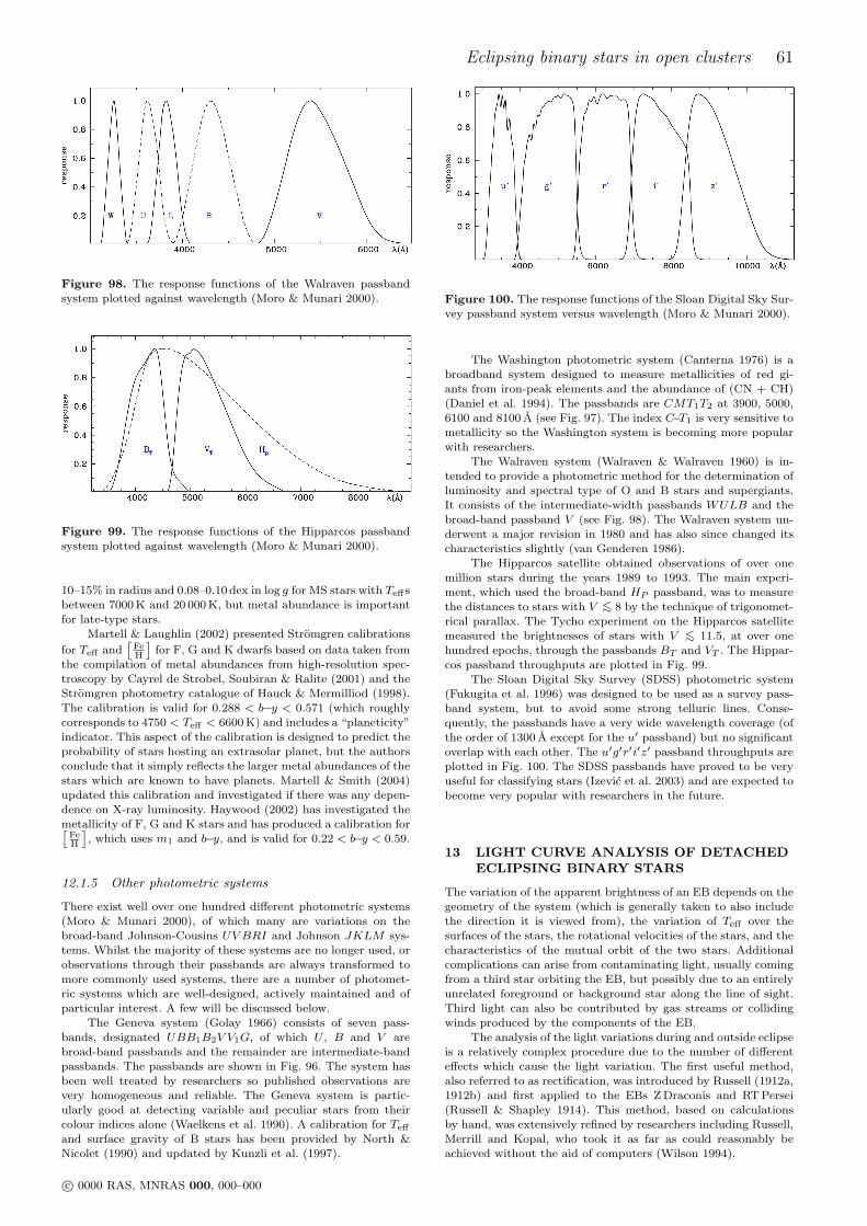
Eclipsing binary stars in open clusters 61
Figure 98. The response functions of the Walraven passbandsystem plotted against wavelength (Moro & Munari 2000).
Figure 99. The response functions of the Hipparcos passbandsystem plotted against wavelength (Moro & Munari 2000).
10–15% in radius and 0.08–0.10 dex in log g for MS stars with Teffsbetween 7000 K and 20 000 K, but metal abundance is importantfor late-type stars.
Martell & Laughlin (2002) presented Stromgren calibrations
for Teff and[
FeH
]for F, G and K dwarfs based on data taken from
the compilation of metal abundances from high-resolution spec-troscopy by Cayrel de Strobel, Soubiran & Ralite (2001) and theStromgren photometry catalogue of Hauck & Mermilliod (1998).The calibration is valid for 0.288 < b−y < 0.571 (which roughlycorresponds to 4750 < Teff < 6600 K) and includes a “planeticity”indicator. This aspect of the calibration is designed to predict theprobability of stars hosting an extrasolar planet, but the authorsconclude that it simply reflects the larger metal abundances of thestars which are known to have planets. Martell & Smith (2004)updated this calibration and investigated if there was any depen-dence on X-ray luminosity. Haywood (2002) has investigated themetallicity of F, G and K stars and has produced a calibration for[
FeH
], which uses m1 and b−y, and is valid for 0.22 < b−y < 0.59.
12.1.5 Other photometric systems
There exist well over one hundred different photometric systems(Moro & Munari 2000), of which many are variations on thebroad-band Johnson-Cousins UV BRI and Johnson JKLM sys-tems. Whilst the majority of these systems are no longer used, orobservations through their passbands are always transformed tomore commonly used systems, there are a number of photomet-ric systems which are well-designed, actively maintained and ofparticular interest. A few will be discussed below.
The Geneva system (Golay 1966) consists of seven pass-bands, designated UBB1B2V V1G, of which U , B and V arebroad-band passbands and the remainder are intermediate-bandpassbands. The passbands are shown in Fig. 96. The system hasbeen well treated by researchers so published observations arevery homogeneous and reliable. The Geneva system is partic-ularly good at detecting variable and peculiar stars from theircolour indices alone (Waelkens et al. 1990). A calibration for Teff
and surface gravity of B stars has been provided by North &Nicolet (1990) and updated by Kunzli et al. (1997).
Figure 100. The response functions of the Sloan Digital Sky Sur-vey passband system versus wavelength (Moro & Munari 2000).
The Washington photometric system (Canterna 1976) is abroadband system designed to measure metallicities of red gi-ants from iron-peak elements and the abundance of (CN + CH)(Daniel et al. 1994). The passbands are CMT1T2 at 3900, 5000,6100 and 8100 A (see Fig. 97). The index C−T1 is very sensitive tometallicity so the Washington system is becoming more popularwith researchers.
The Walraven system (Walraven & Walraven 1960) is in-tended to provide a photometric method for the determination ofluminosity and spectral type of O and B stars and supergiants.It consists of the intermediate-width passbands WULB and thebroad-band passband V (see Fig. 98). The Walraven system un-derwent a major revision in 1980 and has also since changed itscharacteristics slightly (van Genderen 1986).
The Hipparcos satellite obtained observations of over onemillion stars during the years 1989 to 1993. The main experi-ment, which used the broad-band HP passband, was to measurethe distances to stars with V <∼ 8 by the technique of trigonomet-rical parallax. The Tycho experiment on the Hipparcos satellitemeasured the brightnesses of stars with V <∼ 11.5, at over onehundred epochs, through the passbands BT and VT . The Hippar-cos passband throughputs are plotted in Fig. 99.
The Sloan Digital Sky Survey (SDSS) photometric system(Fukugita et al. 1996) was designed to be used as a survey pass-band system, but to avoid some strong telluric lines. Conse-quently, the passbands have a very wide wavelength coverage (ofthe order of 1300 A except for the u′ passband) but no significantoverlap with each other. The u′g′r′i′z′ passband throughputs areplotted in Fig. 100. The SDSS passbands have proved to be veryuseful for classifying stars (Izevic et al. 2003) and are expected tobecome very popular with researchers in the future.
13 LIGHT CURVE ANALYSIS OF DETACHEDECLIPSING BINARY STARS
The variation of the apparent brightness of an EB depends on thegeometry of the system (which is generally taken to also includethe direction it is viewed from), the variation of Teff over thesurfaces of the stars, the rotational velocities of the stars, and thecharacteristics of the mutual orbit of the two stars. Additionalcomplications can arise from contaminating light, usually comingfrom a third star orbiting the EB, but possibly due to an entirelyunrelated foreground or background star along the line of sight.Third light can also be contributed by gas streams or collidingwinds produced by the components of the EB.
The analysis of the light variations during and outside eclipseis a relatively complex procedure due to the number of differenteffects which cause the light variation. The first useful method,also referred to as rectification, was introduced by Russell (1912a,1912b) and first applied to the EBs Z Draconis and RT Persei(Russell & Shapley 1914). This method, based on calculationsby hand, was extensively refined by researchers including Russell,Merrill and Kopal, who took it as far as could reasonably beachieved without the aid of computers (Wilson 1994).
c© 0000 RAS, MNRAS 000, 000–000
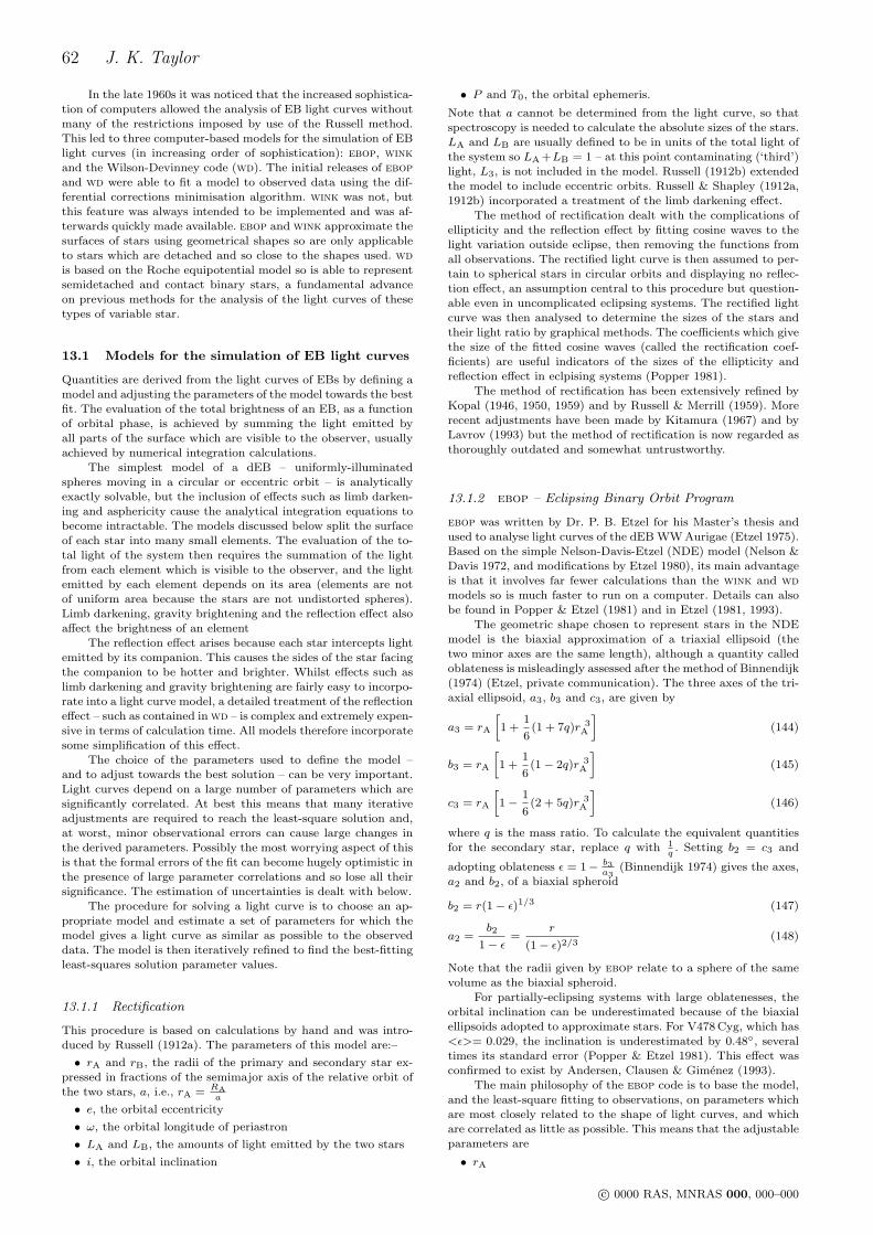
62 J. K. Taylor
In the late 1960s it was noticed that the increased sophistica-tion of computers allowed the analysis of EB light curves withoutmany of the restrictions imposed by use of the Russell method.This led to three computer-based models for the simulation of EBlight curves (in increasing order of sophistication): ebop, winkand the Wilson-Devinney code (wd). The initial releases of ebopand wd were able to fit a model to observed data using the dif-ferential corrections minimisation algorithm. wink was not, butthis feature was always intended to be implemented and was af-terwards quickly made available. ebop and wink approximate thesurfaces of stars using geometrical shapes so are only applicableto stars which are detached and so close to the shapes used. wdis based on the Roche equipotential model so is able to representsemidetached and contact binary stars, a fundamental advanceon previous methods for the analysis of the light curves of thesetypes of variable star.
13.1 Models for the simulation of EB light curves
Quantities are derived from the light curves of EBs by defining amodel and adjusting the parameters of the model towards the bestfit. The evaluation of the total brightness of an EB, as a functionof orbital phase, is achieved by summing the light emitted byall parts of the surface which are visible to the observer, usuallyachieved by numerical integration calculations.
The simplest model of a dEB – uniformly-illuminatedspheres moving in a circular or eccentric orbit – is analyticallyexactly solvable, but the inclusion of effects such as limb darken-ing and asphericity cause the analytical integration equations tobecome intractable. The models discussed below split the surfaceof each star into many small elements. The evaluation of the to-tal light of the system then requires the summation of the lightfrom each element which is visible to the observer, and the lightemitted by each element depends on its area (elements are notof uniform area because the stars are not undistorted spheres).Limb darkening, gravity brightening and the reflection effect alsoaffect the brightness of an element
The reflection effect arises because each star intercepts lightemitted by its companion. This causes the sides of the star facingthe companion to be hotter and brighter. Whilst effects such aslimb darkening and gravity brightening are fairly easy to incorpo-rate into a light curve model, a detailed treatment of the reflectioneffect – such as contained in wd – is complex and extremely expen-sive in terms of calculation time. All models therefore incorporatesome simplification of this effect.
The choice of the parameters used to define the model –and to adjust towards the best solution – can be very important.Light curves depend on a large number of parameters which aresignificantly correlated. At best this means that many iterativeadjustments are required to reach the least-square solution and,at worst, minor observational errors can cause large changes inthe derived parameters. Possibly the most worrying aspect of thisis that the formal errors of the fit can become hugely optimistic inthe presence of large parameter correlations and so lose all theirsignificance. The estimation of uncertainties is dealt with below.
The procedure for solving a light curve is to choose an ap-propriate model and estimate a set of parameters for which themodel gives a light curve as similar as possible to the observeddata. The model is then iteratively refined to find the best-fittingleast-squares solution parameter values.
13.1.1 Rectification
This procedure is based on calculations by hand and was intro-duced by Russell (1912a). The parameters of this model are:–
• rA and rB, the radii of the primary and secondary star ex-pressed in fractions of the semimajor axis of the relative orbit ofthe two stars, a, i.e., rA = RA
a
• e, the orbital eccentricity
• ω, the orbital longitude of periastron
• LA and LB, the amounts of light emitted by the two stars
• i, the orbital inclination
• P and T0, the orbital ephemeris.
Note that a cannot be determined from the light curve, so thatspectroscopy is needed to calculate the absolute sizes of the stars.LA and LB are usually defined to be in units of the total light ofthe system so LA +LB = 1 – at this point contaminating (‘third’)light, L3, is not included in the model. Russell (1912b) extendedthe model to include eccentric orbits. Russell & Shapley (1912a,1912b) incorporated a treatment of the limb darkening effect.
The method of rectification dealt with the complications ofellipticity and the reflection effect by fitting cosine waves to thelight variation outside eclipse, then removing the functions fromall observations. The rectified light curve is then assumed to per-tain to spherical stars in circular orbits and displaying no reflec-tion effect, an assumption central to this procedure but question-able even in uncomplicated eclipsing systems. The rectified lightcurve was then analysed to determine the sizes of the stars andtheir light ratio by graphical methods. The coefficients which givethe size of the fitted cosine waves (called the rectification coef-ficients) are useful indicators of the sizes of the ellipticity andreflection effect in eclpising systems (Popper 1981).
The method of rectification has been extensively refined byKopal (1946, 1950, 1959) and by Russell & Merrill (1959). Morerecent adjustments have been made by Kitamura (1967) and byLavrov (1993) but the method of rectification is now regarded asthoroughly outdated and somewhat untrustworthy.
13.1.2 ebop – Eclipsing Binary Orbit Program
ebop was written by Dr. P. B. Etzel for his Master’s thesis andused to analyse light curves of the dEB WW Aurigae (Etzel 1975).Based on the simple Nelson-Davis-Etzel (NDE) model (Nelson &Davis 1972, and modifications by Etzel 1980), its main advantageis that it involves far fewer calculations than the wink and wdmodels so is much faster to run on a computer. Details can alsobe found in Popper & Etzel (1981) and in Etzel (1981, 1993).
The geometric shape chosen to represent stars in the NDEmodel is the biaxial approximation of a triaxial ellipsoid (thetwo minor axes are the same length), although a quantity calledoblateness is misleadingly assessed after the method of Binnendijk(1974) (Etzel, private communication). The three axes of the tri-axial ellipsoid, a3, b3 and c3, are given by
a3 = rA
[1 +
1
6(1 + 7q)r 3
A
](144)
b3 = rA
[1 +
1
6(1− 2q)r 3
A
](145)
c3 = rA
[1− 1
6(2 + 5q)r 3
A
](146)
where q is the mass ratio. To calculate the equivalent quantitiesfor the secondary star, replace q with 1
q. Setting b2 = c3 and
adopting oblateness ε = 1− b3a3
(Binnendijk 1974) gives the axes,a2 and b2, of a biaxial spheroid
b2 = r(1− ε)1/3 (147)
a2 =b2
1− ε=
r
(1− ε)2/3(148)
Note that the radii given by ebop relate to a sphere of the samevolume as the biaxial spheroid.
For partially-eclipsing systems with large oblatenesses, theorbital inclination can be underestimated because of the biaxialellipsoids adopted to approximate stars. For V478 Cyg, which has<ε>= 0.029, the inclination is underestimated by 0.48, severaltimes its standard error (Popper & Etzel 1981). This effect wasconfirmed to exist by Andersen, Clausen & Gimenez (1993).
The main philosophy of the ebop code is to base the model,and the least-square fitting to observations, on parameters whichare most closely related to the shape of light curves, and whichare correlated as little as possible. This means that the adjustableparameters are
• rA
c© 0000 RAS, MNRAS 000, 000–000

Eclipsing binary stars in open clusters 63
• k = rBrA
, the ratio of the stellar radii (where rB is the radius
of the secondary star)
• J = JBJA
, the surface brightness ratio where JA and JB are
the central surface brightnesses of the primary and secondary starrespectively
• L3
• i
• q
• uA and uB, the linear limb darkening coefficient for each star
• βA and βB, the gravity brightening exponent for each star
• e sinω
• e cosω
The orbital period, P , and reference time of primary eclipse mind-minimum, T0, are also required but must be fixed during least-squares fitting by differential corrections. Another two parame-ters, the outside-eclipse light of the system and the phase differ-ence between the midpoint of primary eclipse and phase zero, arealso needed to place the light curve properly in parameter space.
The quantities e sinω and e cosω, rather than e and ω, havebeen chosen as model parameters because they tend to be betterdetermined when the orbit is only slightly eccentric (Etzel 1993).To a first approximation, e cosω depends on the phase of midpointof secondary eclipse and e sinω depends on the relative durationsof the eclipses. More formally, and ignoring terms in eccentricityto powers greater than one,
e cosω ≈ π(φMin II − 0.5)
1 + cosec2i(149)
where φMin II is the phase difference between secondary minimumand the immediately preceding primary minimum (Gudur 1978).Zakirov (2001) gives the ratio of the durations of secondary andprimary eclipses to be
δφ(Min II)
δφ(Min I)=
1 + e sinω
1− e sinω(150)
e sinω is generally less well-determined than e cosω, although theopposite situation exists in the calculation of spectroscopic orbits(Sec. 11).
Limb darkening is incorporated in ebop using the linear law(Sec. 1.4.1, eq. 29) – the simple nature of the NDE models meansthat more complex limb darkening laws are of limited impor-tance. However, their inclusion is advantageous and has been im-plemented by A. Gimenez and J. Dıaz-Cordoves. Their revisedversion of ebop also has a slightly improved geometrical basisand the ability to allow for apsidal motion (7.2), and was usedby Gimenez & Quintana (1992) in a study of the eccentric dEBV477 Cygni.
The reflection effect in ebop is dealt with in a very simplebolometric manner based on Binnendijk (1960) and is usuallycalculated from the geometry of the system being analysed. Thisapproximation becomes less accurate when the Teffs of the twostars are very different or vary significantly over the stellar sur-faces, but in any case it is not recommended to use ebop forsystems with a significant reflection effect (Etzel 1980).
The proximity effects (reflection and asphericity) are notincluded in the calculation of the light lost during eclipse, soonly well-detached systems, where the change in proximity effectsthroughout eclipse is negligible, can be studied.
Popper & Etzel (1981) find that the NDE model and theebop code are trustworthy for stars with oblateness ε < 0.04. Be-yond this point, biaxial ellipsoids are unable to satisfactorily ap-proximate the shape of the distorted star. North & Zahn (2004b)studied dEBs in the Magellanic Clouds using ebop and wd. Theyfound that for average fractional radii of 0.25 and 0.3, the radiiderived using ebop were 1% and 5% different, respectively, to theradii found using wd. These studies provide good estimates of thelimits of applicability of ebop. A study of the LMC dEB HV 2274by Watson et al. (1992) found that the differences between anebop and wink solution were minor for this system, for whichrA + rB ≈ 0.5.
13.1.3 wink
The wink light curve model was written by D. B. Wood (Wood1971a, 1972) and made available to the astronomical community(Wood 1973b). It is a geometrical model which approximates thesurfaces of stars with triaxial ellipsoids (equations 144, 145 and146 in previous section) and incorporates the model parameters:–
• P and T0
• a
• e cosω
• e sinω
• i
• q
• aA, bA, cA, the fractional semiaxes of the primary star
• aB, bB, cB, the fractional semiaxes of the secondary star
• IA, IB, the central surface brightnesses at quadrature
• L3
• uA, uB
• βA, βB
• wA, wB, the reflection coefficient (albedo) for each star
The model is fitted to observations using the method of differen-tial corrections.
The six stellar semiaxes are actually replaced in the modelby the dimensionless quantities rA, k, εA, εB, ζA and ζB where
aA = rAa (151)
aB = krAa (152)
bA = εArAa (153)
bB = εBkrAa (154)
cA = (1 + ζA)ε 2A rAa (155)
cB = (1 + ζB)ε 2B krAa (156)
Here the rA is the fractional major semiaxis of the primary starand k is effectively the ratio of the radii. The ε are the elliptic-ities in the ab (orbital) plane and the ζ measure how much theellipticities in the bc plane differ from those in the ab plane.
Limb darkening is included using the linear law (Sec. 1.4.1),as with ebop. Gravity brightening is defined in a similar mannerwith the equation
I = I0
[1− β + β
(r
r0
)](157)
where I0 is the central surface brightness, r is the local radiusand r0 is the radius of the central point of the stellar disc. Thisdefinition means that β is aproximately four times the quantityreferred to as β1 in Sec. 1.5.
The initial treatment of reflection (Wood 1971a) was to cal-culate the amount of light incident at a point on the surfaceand to reradiate some fraction w of it. A more advanced treat-ment was incorporated by Wood (1973a) but was shown to stillbe inadequate for high-precision work. Synchronous rotation wasinitially assumed but the effects of rotation were subsequentlyadded. wink corrects the stellar radii for the expansion effectsdue to rotation (Clausen et al. 2003) whereas wd does not.
13.1.4 The Wilson-Devinney (wd) code
The wd code is probably the most commonly used light curveanalysis code, partly due to its much greater sophistication com-pared to ebop and wink. Rather than modelling the discs of starsusing geometrical shapes, the components of a binary systemare modelled in three dimensions using the Roche prescriptionof equipotential surfaces. This is implemented by defining pointson the surface of the star, distributed approximately uniformlyin a spherical coordinate system. The number of points is of theorder of one thousand per star, although the wd code allows theuser to choose the approximate amount.
Adoption of the Roche model for calculating the shapes and
c© 0000 RAS, MNRAS 000, 000–000
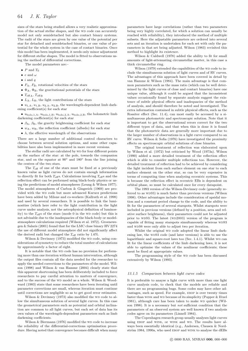
64 J. K. Taylor
sizes of the stars being studied allows a very realistic approxima-tion of the actual stellar shapes, and the wd code can accuratelymodel not only semidetached but also contact binary systems.The radii of the stars are given by one value of the potential perstar for detached and semidetached binaries, or one value of po-tential for the whole system in the case of contact binaries. Oncethis model has been implemented, it needs only minor adjustmentfor different stellar shapes. The model is fitted to observations us-ing the method of differential corrections.
The model parameters are:–
• P and T0
• e and ω
• i and q
• FA, FB, rotational velocities of the stars
• ΦA, ΦB, the gravitational potentials of the stars
• TeffA, TeffB
• LA, LB, the light contributions of the stars
• u1,A, u1,B, u2,A, u2,B, the wavelength-dependent limb dark-ening coefficient(s) for each star
• ubolo,1,A, ubolo,1,B, ubolo,2,A, ubolo,2,B, the bolometric limbdarkening coefficient(s) for each star
• βA, βB, the gravity brightening coefficient for each star
• wA, wB, the reflection coefficient (albedo) for each star
• λ, the effective wavelength of the observations
There are a large number of additional control characters tochoose between several solution options, and some other capa-bilities have also been implemented in more recent versions.
The stellar radii are calculated by wd for four different pointson the surface of the star: at the pole, towards the companionstar, and on the equator at 90 and 180 from the line joiningthe centres of the two stars.
The Teff of one of the stars must be fixed at a previouslyknown value as light curves do not contain enough informationto directly fit for both Teffs. Calculations involving Teffs and thereflection effect can be performed using black-body physics or us-ing the predictions of model atmospheres (Leung & Wilson 1977).The model atmospheres of Carbon & Gingerich (1969) are pro-vided with the wd code but more advanced Kurucz predictionshave been added by Milone and co-workers (Kallrath et al. 1998)and used by several researchers. It is possible to link the lumi-nosities (which here refer to the light contribution in the lightcurve under analysis, not the astrophysical definition of luminos-ity) to the Teffs of the stars (mode 0 in the wd code) but this isnot advisable due to the inadequacies of the black-body or model-atmosphere calculations required (Wilson et al. 1972). Groenewe-gen & Salaris (2001) found that for the LMC close binary HV 2274the use of different model atmosphere did not significantly affectthe derived radii but changed the Teff ratio by 1.6%.
Wilson & Devinney (1973) modified the wd code, using con-siderations of symmetry to reduce the total number of calculationsby approximately a factor of eight.
It is notable that the wd code has no provision for perform-ing more than one iteration without human intervention, althoughthe output files contain all the data needed for the researcher toapply the needed corrections to the parameters of the model. Wil-son (1998) and Wilson & van Hamme (2004) clearly state thatthis apparent shortcoming has been deliberately included to forceresearchers to pay careful attention to matters of convergence,and to the success of the wd model as a whole. Wilson & Wood-ward (1983) state that some researchers have been iterating untilparameter corrections are small, whereas iteration must continueuntil corrections are negligible so as to get good error estimates.
Wilson & Devinney (1973) also modified the wd code to al-low the simultaneous solution of several light curves. In this casethe geometrical parameters such as potential and orbital inclina-tion are common to all light curves, but each set of data has itsown values of the wavelength-dependent parameters such as limbdarkening coefficients.
Wilson & Biermann (1976) modified the wd code to increasethe reliability of the differential-corrections optimisation proce-dure. Having noted that convergence becomes difficult when many
parameters have large correlations (rather than two parametersbeing very highly correlated, for which a solution can usually bereached with reliability), they introduced the method of multiplesubsets. Here the adjustable parameters are ordered into severalsets and an iteration is undertaken for each set with only the pa-rameters in that set being adjusted. Wilson (1983) revisited thismethod to highlight its existence.
Wilson & Caldwell (1978) added the ability to fit for smallamounts of light-attenuating circumstellar matter, in this case athick circumstellar ring.
Wilson (1979) extended the capabilities of the wd code to in-clude the simultaneous solution of light curves and of RV curves.The advantages of this approach have been covered in detail byvan Hamme & Wilson (1984). The main advantage is that com-mon parameters such as the mass ratio (which can be well deter-mined by the light curves of close and contact binaries) have oneunique value, although it could be argued that the inconsistentvalues occasionally found by separate analysis suggest the exis-tence of subtle physical effects and inadequacies of the methodof analysis, and should therefore be noted and investigated. Theextra information contained in subtle physical effects, such as theRossiter effect (Sec. 11.4), can most easily be accessed by a si-multaneous photometric and spectroscopic solution. Note that itis important to get the observational errors correct for the twodifferent types of data, and that when this is done it is foundthat the photometric data are generally more important due tothe larger number of observations in a light curve compared to anRV curve. Wilson & Sofia (1976) have investigated the proximityeffects on spectroscopic orbital solutions of close binaries.
The original treatment of reflection was elaborated uponby Wilson et al. (1972) but criticised by Wood (1973a). Wilson(1990) added a more detailed treatment of the reflection effectwhich is able to consider multiple reflections too. However, thedetailed treatment of reflection had to be achieved by consideringthe light incident from each surface element on one star to eachsurface element on the other star, so can be very expensive interms of computing time when analysing eccentric systems. Thisis because the reflection effect in eccentric EBs is dependent onorbital phase, so must be calculated once for every datapoint.
The 1993 version of the Wilson-Devinney code (generally re-ferred to as wd93) is much faster than previous versions (Wilson1998). Other advantages include the consideration of apsidal mo-tion and a constant period change to the code, and the ability tofit for the parameters of several starspots. Whilst starspots wereincluded in previous versions (defined by a position, area and rel-ative surface brightness), their parameters could not be adjustedprior to wd93. The latest (wd2003) version of the program iscapable of fitting many starspots simultaneously whereas wd93and wd98 were only able to adjust two per iteration.
Whilst the original wd code adopted the linear limb dark-ening law, the wd93 code (and later versions) is able to use thelogarithmic and square-root laws too (Sec. 1.4.1). Whilst wd canfit for the linear coefficients of the limb darkening laws, it is notable to optimise the values of the nonlinear coefficients; thesemsut be fixed at appropriate values.
The programming style of the wd code has been discussedextensively by Wilson (1993).
13.1.5 Comparison between light curve codes
It is preferable to anayse a light curve with more than one lightcurve analysis code, to check that the models are reliable andthere are no programming bugs. Some codes may have other ad-vantages, such as speed. For example, ebop is over twenty timesfaster than wink and wd because of its simplicity (Popper & Etzel1981), although care has been taken to make wd quicker (Wil-son 1998). It is a necessary but not sufficient condition that theparameters of an observed system are well known if two analysiscodes agree on its parameters (Linnell 1984).
The Copenhagen research group usually analyses light curvesusing ebop and wink, or wink and wd. The results have al-ways been essentially identical (e.g., Andersen, Clausen & Nord-strom 1984, 1990a, who used ebop and wink to analyse the dEBs
c© 0000 RAS, MNRAS 000, 000–000
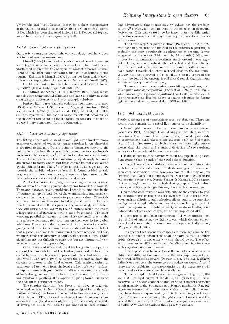
Eclipsing binary stars in open clusters 65
VV Pyxidis and V1031 Orionis) except for a slight disagreementin the value of orbital inclination (Andersen, Clausen & Gimenez1993), which has been discussed in Sec. 13.1.2. Popper (1980) alsonotes that ebop and wink agree very well.
13.1.6 Other light curve fitting codes
Quite a few computer-based light curve analysis tools have beenwritten and used by researchers.
Linnell (1984) introduced a physical model based on numer-ical integration between points on a surface. This model is so-phisticated enough for the analysis of contact binaries (Linnell1986) and has been equipped with a simplex least-squares fittingroutine (Kallrath & Linnell 1987), but has not been widely used.It is more complex than the wd code (Kallrath & Linnell 1987).
G. Hill has constructed the light curve model light, followedby light2 (Hill & Hutchings 1970; Hill 1979).
P. Hadrava has written fotel (Hadrava 1990, 1995), whichmodels stars using triaxial ellipsoids and has the ability to makesimultaneous photometric and spectroscopic solutions.
Further light curve analysis codes are mentioned in Linnell(1984) and Wilson (1994). Lorentz, Mayer & Drechsel (1998)use the code moro (Drechsel et al. 1995) to study the dEBSZ Camelopardalis. This code is based on wd but accounts forthe change in radius caused by the radiation pressure incident ona close binary component from its companion.
13.1.7 Least-squares fitting algorithms
The fitting of a model to an observed light curve involves manyparameters, some of which are quite correlated. An algorithmis required to navigate from a point in parameter space to thepoint where the best fit occurs. It is instructive to visualise thisproblem in the form of a χ2 surface in two dimensions, althoughit must be remembered there are usually significantly far moredimensions to worry about and these cannot be easily visualisedby the human brain. The χ2 surface is high at its edges and lowtowards the middle, where the best fit is found. Added to thislarge-scale form are many valleys, bumps and dips, caused by theparameters correlations and observational errors.
All least-squares fitting algorithms navigate in steps (iter-ations) from the starting parameter values towards the best fit.There are, however, several problems. Large local gradients in theχ2 surface can give a bad idea of the overall surface and cause ex-cessive adjustments to be made to parameter values. Often thiswill result in values diverging to infinity and causing the solu-tion to break down. If two parameters are strongly correlated,they will cause a deep valley in the χ2 surface which can causea large number of iterations until a good fit is found. The mostworrying possibility, though, is that there are small dips in theχ2 surface which can catch solutions on their way to the globalminimum. These local minima can be difficult to detect and oftengive plausible results. In many cases it is difficult to be confidentthat a global, and not local, minimum has been reached, and alsowhether or not this difficulty is actually important. Global searchalgorithms are not difficult to construct but are impractically ex-pensive in terms of computer time.
ebop, wink and wd are all capable of adjusting the param-eters of their models to find the least-squares best fit to an ob-served light curve. They use the process of differential corrections(see Wyse 1939; Irwin 1947) to adjust the parameters from thestarting estimates to the final solution. This method estimatesparameter adjustments from the local gradient of the χ2 surface.It requires reasonably good initial conditions because it is capableof both divergence and of settling in local minima (it is a localminimisation algorithm). It is capable of giving formal errors onthe final fitted parameter values.
The simplex algorithm (see Press et al. 1992, p. 402, whohave implemented the Nelder-Mead simplex algorithm in the sub-routine amoeba) has been implemented in the wd code by Kall-rath & Linnell (1987). As used by these authors it has some char-acteristics of a global search algorithm; it is certainly incapableof divergence but is still able to get trapped in local minima.
One advantage is that it uses only χ2 values, not the gradientof the χ2 surface, so does not require the calculation of partialderivatives. This can cause it to be faster than the differentialcorrections process, but it may often require more iterations sowill be slower.
The Levenberg-Marquardt method (Press et al. 1992, p. 678,who have implemented the method in the mrqmin algorithm) isprobably the most popular fitting algorithm at present. It wassuggested by Levenberg (1944) and by Marquardt (1963), andutilises two minimisation algorithms simultaneously, one algo-rithm being slow and robust, the other fast and less reliable.The former method is used far from minimum, with a contin-uous switch towards the latter method close to the minimum.mrqmin also has a provision for calculating formal errors of thefit (but see Sec. 13.3). mrqmin is still a local search algorithm andis technically capable of diverging.
There are many more least-squares fitting algorithms, suchas singular value decomposition (Press et al. 1992, p. 670), simu-lated annealing and genetic algorithms (Ford 2003) available, butthe three methods detailed above are quite adequate for fittinglight curve models to observed data (Wilson 1994).
13.2 Solving light curves
Firstly a decent set of observations must be obtained. There areseveral requirements for a set of light curves to be definitive:–
• Good light curves in two or more passbands are needed(Andersen 1991), although I would suggest that data in threepassbands has become the minimum requirement, preferablyin intermediate band photometric systems such as Stromgren(Sec. 12.1.3). Separately analysing three or more light curvesmeans that the mean and standard deviation of the resultingvalues can be calculated for each parameter.
• Both eclipses must be covered without any gaps in the phaseddata greater than a tenth of the total eclipse duration.
• The eclipses must contain at least one hundred datapointswith low observational errors. If limb darkening is to be studiedthen each observation must have an error of 0.005 mag or less(Popper 1984, 2000) for simple systems. More complicated dEBswill require better data. North, Studer & Kunzli (1997) suggestthat meaningful results for limb darkening require five hundredpoints per eclipse, although this may be a little conservative.
• Sufficient data must be available outside the eclipses to givean accurate reference brightness, to cover any outside-eclipse vari-ation such as ellipticity and reflection effects, and to be sure thatno significant complications could exist without being noticed. Aminimum requirement is perhaps twenty accurate and well-spaceddatapoints between each eclipse for an uncomplicated dEB.
• There are no significant night errors. If they are present thenthe results of analysing the light curves, which depend on ob-servational errors being random, could be systematically wrong(Popper & Etzel 1981).
It appears that secondary eclipses are more sensitive to thevariation of model parameters than primary eclipses (Popper1986) although it is not clear why this should be so. The effectwill be smaller for dEBs composed of similar stars than for thosewith very dissimilar components.
It is a good idea to have two different sets of observationsobtained at different times and with different equipment, and pos-sibly with different observers (Popper 1981). This can highlightdifficulties such as night errors or data reduction errors. Also, ifthere are no problems, the uncertainties on the parameters willbe reduced as there are more data available.
Three example sets of light curves are given in Figs. 101, 102and 103. The light curves of the dEB GG Lupi in Fig. 101 wereobserved using a four-channel photoelectric photometer observingsimultaneously in the Stromgren u, v, b and y passbands. Fig. 102shows an example of a light curve which is not definitive andmay have been compromised by difficult observing conditions.Fig. 103 shows the most complete light curve obtained (until theyear 2002), consisting of 5759 robotic-telescope observations ofthe dEB WW Camelopardalis through a V passband.
c© 0000 RAS, MNRAS 000, 000–000
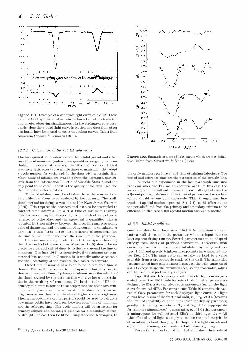
66 J. K. Taylor
Figure 101. Example of a definitive light curve of a dEB. Thesedata, of GG Lupi, were taken using a four-channel photoelectricphotometer observing simultaneously in the Stromgren uvby pass-bands. Here the y-band light curve is plotted and data from otherpassbands have been used to construct colour curves. Taken fromAndersen, Clausen & Gimenez (1993).
13.2.1 Calculation of the orbital ephemeris
The first quantities to calculate are the orbital period and refer-ence time of minimum (unless these quantities are going to be in-cluded in the overall fit using e.g., the wd code). For most dEBs itis entirely satisfactory to assemble times of minimum light, adopta cycle number for each, and fit the data with a straight line.Many times of minima are available from the literature, particu-larly from the Information Bulletin of Variable Stars36, and theonly point to be careful about is the quality of the data used andthe method of determination.
Times of minima must be obtained from the observationaldata which are about to be analysed by least-squares. The tradi-tional method for doing so was outlined by Kwee & van Woerden(1956). This requires the observational data to be resampled toconstant time intervals. For a trial time of minimum (halfwaybetween two resampled datapoints), one branch of the eclipse isreflected onto the other and the agreement is quantified. This isrepeated for times midway between the preceding and proceedingpairs of datapoints and the amount of agreement is calculated. Aparabola is then fitted to the three measures of agreement andthe time of minimum found from the minimum of the parabola.
If the minima are asymmetric (due to the shape of the orbit)then the method of Kwee & van Woerden (1956) should be re-placed by a parabola fitted directly to the data around the time ofminimum (Gimenez 1985). Alternatively, if the minima are sym-metrical but not total, a Gaussian fit is usually quite acceptableand the uncertainty of the result is then easier to estimate.
Once times of minima have been found, a reference time ischosen. The particular choice is not important but it is best tochoose an accurate time of primary minimum near the middle ofthe times covered by the data, as this will give lower uncertain-ties in the resulting reference time, T0. In the study of EBs theprimary minimum is defined to be deeper than the secondary min-imum, so in general refers to a transit of the star of lower surfacebrightness across the disc of the star of higher surface brightness.Then an approximate orbital period should be used to calculatehow many orbits have occurred between each time of minimumand the reference time. This cycle number will be an integer forprimary eclipses and an integer plus 0.5 for a secondary eclipse.A straight line can then be fitted, using standard techniques, to
36 http://www.konkoly.hu/IBVS/IBVS.html
Figure 102. Example of a set of light curves which are not defini-tive. Taken from Srivastava & Sinha (1985).
the cycle numbers (ordinate) and time of minima (abscissa). Theperiod and reference time are the parameters of the straight line.
The technique expounded in the last paragraph runs intoproblems when the EB has an eccentric orbit. In this case thesecondary minima will not in general occur halfway between theadjacent primary minima and the times of primary and secondaryeclipse should be analysed separately. This, though, runs intotrouble if apsidal motion is present (Sec. 7.2), as this effect causesthe periods found from the primary and secondary minima to bedifferent. In this case a full apsidal motion analysis is needed.
13.2.2 Initial conditions
Once the data have been assembled it is important to esti-mate a realistic set of initial parameter values to input into theleast-squares fitting routine. Several parameters can be adopteddirectly from theory or previous observation. Theoretical limbdarkening coefficients have been tabulated by many authors(Sec. 1.4.1) and gravity brightening exponents have expected val-ues (Sec. 1.5). The mass ratio can usually be fixed to a valueavailable from a spectroscopic study of the dEB. The quantitiesjust mentioned have only a minor impact on the light variation ofa dEB except in specific circumstances, so any reasonable valuescan be used for a preliminary analysis.
Figs. 104 and 105 display a set of model light curves gen-erated using the ebop code for sets of photometric parametersdesigned to illustrate the effect each parameter has on the lightcurve for typical dEBs. For convenience Table 10 contains the val-ues of these parameters for each displayed light curve. All lightcurves have: a sum of the fractional radii, rA +rB, of 0.4 (towardsthe limit of capability of ebop but chosen for display purposes);gravity brightening coefficients, βA and βB, of 1.0 (appropriatefor radiative atmospheres); a mass ratio, q, of 1.0 (this parameteris unimportant for well-detached EBs); no third light, L3 = 0.0(the effect of third light is simply to reduce the total magnitudeof variation without changing the shape of the light curve); andequal limb darkening coefficients for both stars, uA = uB.
Panels (a), (b) and (c) of Fig. 104 each show three sets of
c© 0000 RAS, MNRAS 000, 000–000
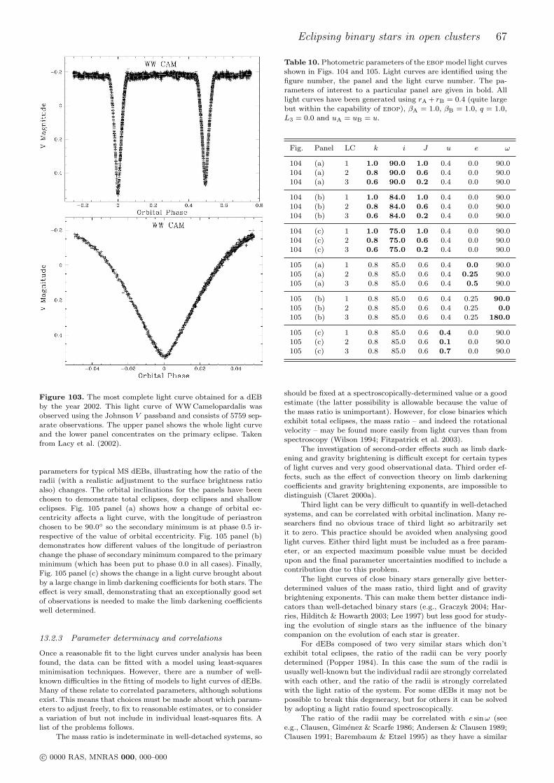
Eclipsing binary stars in open clusters 67
Figure 103. The most complete light curve obtained for a dEBby the year 2002. This light curve of WW Camelopardalis wasobserved using the Johnson V passband and consists of 5759 sep-arate observations. The upper panel shows the whole light curveand the lower panel concentrates on the primary eclipse. Takenfrom Lacy et al. (2002).
parameters for typical MS dEBs, illustrating how the ratio of theradii (with a realistic adjustment to the surface brightness ratioalso) changes. The orbital inclinations for the panels have beenchosen to demonstrate total eclipses, deep eclipses and shalloweclipses. Fig. 105 panel (a) shows how a change of orbital ec-centricity affects a light curve, with the longitude of periastronchosen to be 90.0 so the secondary minimum is at phase 0.5 ir-respective of the value of orbital eccentricity. Fig. 105 panel (b)demonstrates how different values of the longitude of periastronchange the phase of secondary minimum compared to the primaryminimum (which has been put to phase 0.0 in all cases). Finally,Fig. 105 panel (c) shows the change in a light curve brought aboutby a large change in limb darkening coefficients for both stars. Theeffect is very small, demonstrating that an exceptionally good setof observations is needed to make the limb darkening coefficientswell determined.
13.2.3 Parameter determinacy and correlations
Once a reasonable fit to the light curves under analysis has beenfound, the data can be fitted with a model using least-squaresminimisation techniques. However, there are a number of well-known difficulties in the fitting of models to light curves of dEBs.Many of these relate to correlated parameters, although solutionsexist. This means that choices must be made about which param-eters to adjust freely, to fix to reasonable estimates, or to considera variation of but not include in individual least-squares fits. Alist of the problems follows.
The mass ratio is indeterminate in well-detached systems, so
Table 10. Photometric parameters of the ebop model light curvesshown in Figs. 104 and 105. Light curves are identified using thefigure number, the panel and the light curve number. The pa-rameters of interest to a particular panel are given in bold. Alllight curves have been generated using rA + rB = 0.4 (quite largebut within the capability of ebop), βA = 1.0, βB = 1.0, q = 1.0,L3 = 0.0 and uA = uB = u.
Fig. Panel LC k i J u e ω
104 (a) 1 1.0 90.0 1.0 0.4 0.0 90.0104 (a) 2 0.8 90.0 0.6 0.4 0.0 90.0104 (a) 3 0.6 90.0 0.2 0.4 0.0 90.0
104 (b) 1 1.0 84.0 1.0 0.4 0.0 90.0104 (b) 2 0.8 84.0 0.6 0.4 0.0 90.0104 (b) 3 0.6 84.0 0.2 0.4 0.0 90.0
104 (c) 1 1.0 75.0 1.0 0.4 0.0 90.0104 (c) 2 0.8 75.0 0.6 0.4 0.0 90.0104 (c) 3 0.6 75.0 0.2 0.4 0.0 90.0
105 (a) 1 0.8 85.0 0.6 0.4 0.0 90.0105 (a) 2 0.8 85.0 0.6 0.4 0.25 90.0105 (a) 3 0.8 85.0 0.6 0.4 0.5 90.0
105 (b) 1 0.8 85.0 0.6 0.4 0.25 90.0105 (b) 2 0.8 85.0 0.6 0.4 0.25 0.0105 (b) 3 0.8 85.0 0.6 0.4 0.25 180.0
105 (c) 1 0.8 85.0 0.6 0.4 0.0 90.0105 (c) 2 0.8 85.0 0.6 0.1 0.0 90.0105 (c) 3 0.8 85.0 0.6 0.7 0.0 90.0
should be fixed at a spectroscopically-determined value or a goodestimate (the latter possibility is allowable because the value ofthe mass ratio is unimportant). However, for close binaries whichexhibit total eclipses, the mass ratio – and indeed the rotationalvelocity – may be found more easily from light curves than fromspectroscopy (Wilson 1994; Fitzpatrick et al. 2003).
The investigation of second-order effects such as limb dark-ening and gravity brightening is difficult except for certain typesof light curves and very good observational data. Third order ef-fects, such as the effect of convection theory on limb darkeningcoefficients and gravity brightening exponents, are impossible todistinguish (Claret 2000a).
Third light can be very difficult to quantify in well-detachedsystems, and can be correlated with orbital inclination. Many re-searchers find no obvious trace of third light so arbitrarily setit to zero. This practice should be avoided when analysing goodlight curves. Either third light must be included as a free param-eter, or an expected maximum possible value must be decidedupon and the final parameter uncertainties modified to include acontribution due to this problem.
The light curves of close binary stars generally give better-determined values of the mass ratio, third light and of gravitybrightening exponents. This can make them better distance indi-cators than well-detached binary stars (e.g., Graczyk 2004; Har-ries, Hilditch & Howarth 2003; Lee 1997) but less good for study-ing the evolution of single stars as the influence of the binarycompanion on the evolution of each star is greater.
For dEBs composed of two very similar stars which don’texhibit total eclipses, the ratio of the radii can be very poorlydetermined (Popper 1984). In this case the sum of the radii isusually well-known but the individual radii are strongly correlatedwith each other, and the ratio of the radii is strongly correlatedwith the light ratio of the system. For some dEBs it may not bepossible to break this degeneracy, but for others it can be solvedby adopting a light ratio found spectroscopically.
The ratio of the radii may be correlated with e sinω (seee.g., Clausen, Gimenez & Scarfe 1986; Andersen & Clausen 1989;Clausen 1991; Barembaum & Etzel 1995) as they have a similar
c© 0000 RAS, MNRAS 000, 000–000
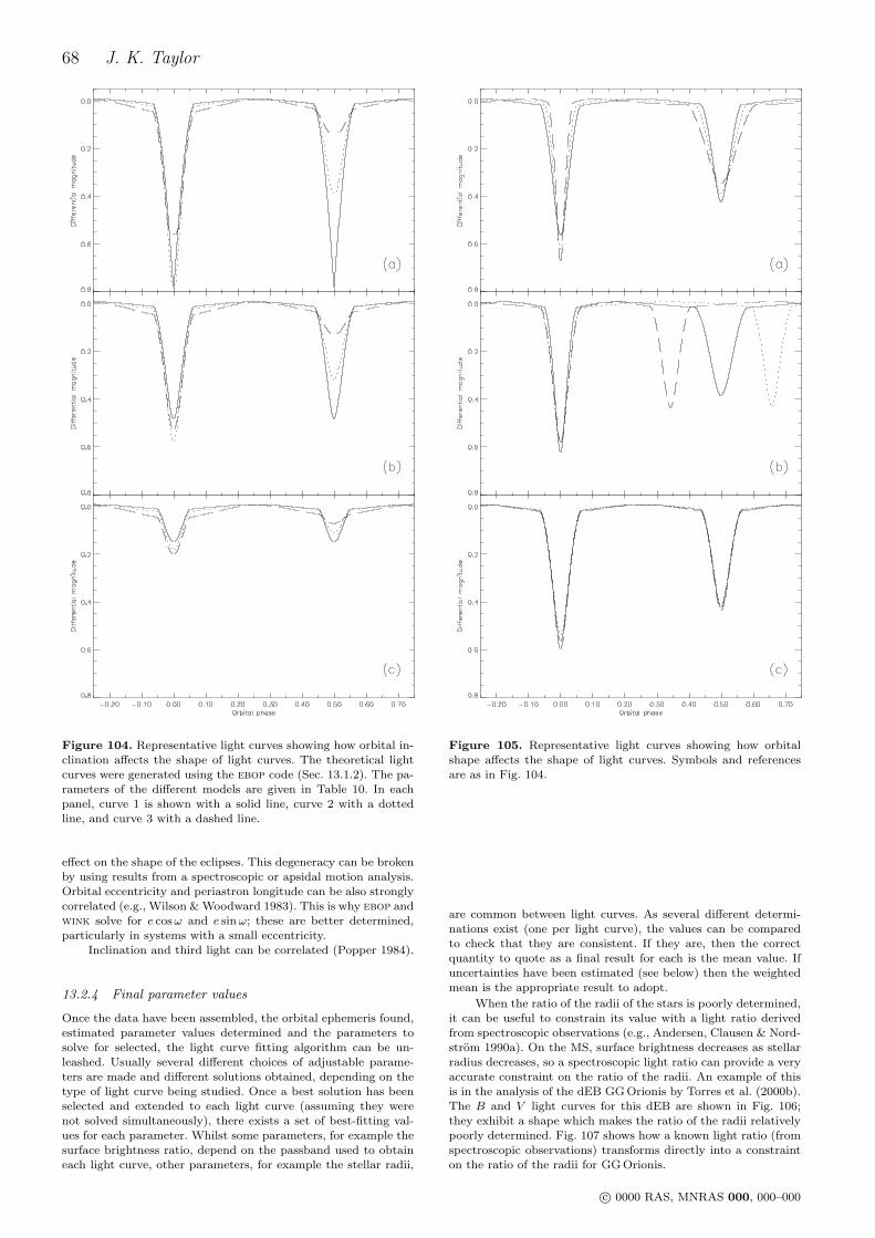
68 J. K. Taylor
Figure 104. Representative light curves showing how orbital in-clination affects the shape of light curves. The theoretical lightcurves were generated using the ebop code (Sec. 13.1.2). The pa-rameters of the different models are given in Table 10. In eachpanel, curve 1 is shown with a solid line, curve 2 with a dottedline, and curve 3 with a dashed line.
effect on the shape of the eclipses. This degeneracy can be brokenby using results from a spectroscopic or apsidal motion analysis.Orbital eccentricity and periastron longitude can be also stronglycorrelated (e.g., Wilson & Woodward 1983). This is why ebop andwink solve for e cosω and e sinω; these are better determined,particularly in systems with a small eccentricity.
Inclination and third light can be correlated (Popper 1984).
13.2.4 Final parameter values
Once the data have been assembled, the orbital ephemeris found,estimated parameter values determined and the parameters tosolve for selected, the light curve fitting algorithm can be un-leashed. Usually several different choices of adjustable parame-ters are made and different solutions obtained, depending on thetype of light curve being studied. Once a best solution has beenselected and extended to each light curve (assuming they werenot solved simultaneously), there exists a set of best-fitting val-ues for each parameter. Whilst some parameters, for example thesurface brightness ratio, depend on the passband used to obtaineach light curve, other parameters, for example the stellar radii,
Figure 105. Representative light curves showing how orbitalshape affects the shape of light curves. Symbols and referencesare as in Fig. 104.
are common between light curves. As several different determi-nations exist (one per light curve), the values can be comparedto check that they are consistent. If they are, then the correctquantity to quote as a final result for each is the mean value. Ifuncertainties have been estimated (see below) then the weightedmean is the appropriate result to adopt.
When the ratio of the radii of the stars is poorly determined,it can be useful to constrain its value with a light ratio derivedfrom spectroscopic observations (e.g., Andersen, Clausen & Nord-strom 1990a). On the MS, surface brightness decreases as stellarradius decreases, so a spectroscopic light ratio can provide a veryaccurate constraint on the ratio of the radii. An example of thisis in the analysis of the dEB GG Orionis by Torres et al. (2000b).The B and V light curves for this dEB are shown in Fig. 106;they exhibit a shape which makes the ratio of the radii relativelypoorly determined. Fig. 107 shows how a known light ratio (fromspectroscopic observations) transforms directly into a constrainton the ratio of the radii for GG Orionis.
c© 0000 RAS, MNRAS 000, 000–000
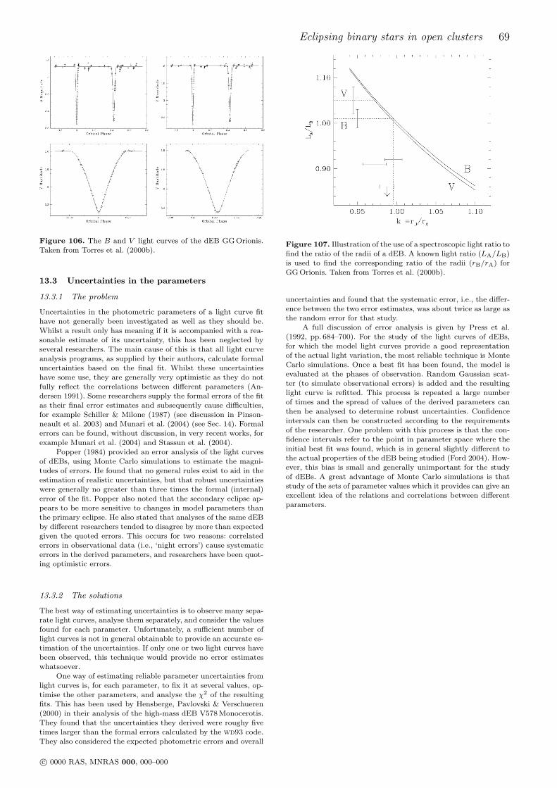
Eclipsing binary stars in open clusters 69
Figure 106. The B and V light curves of the dEB GG Orionis.Taken from Torres et al. (2000b).
13.3 Uncertainties in the parameters
13.3.1 The problem
Uncertainties in the photometric parameters of a light curve fithave not generally been investigated as well as they should be.Whilst a result only has meaning if it is accompanied with a rea-sonable estimate of its uncertainty, this has been neglected byseveral researchers. The main cause of this is that all light curveanalysis programs, as supplied by their authors, calculate formaluncertainties based on the final fit. Whilst these uncertaintieshave some use, they are generally very optimistic as they do notfully reflect the correlations between different parameters (An-dersen 1991). Some researchers supply the formal errors of the fitas their final error estimates and subsequently cause difficulties,for example Schiller & Milone (1987) (see discussion in Pinson-neault et al. 2003) and Munari et al. (2004) (see Sec. 14). Formalerrors can be found, without discussion, in very recent works, forexample Munari et al. (2004) and Stassun et al. (2004).
Popper (1984) provided an error analysis of the light curvesof dEBs, using Monte Carlo simulations to estimate the magni-tudes of errors. He found that no general rules exist to aid in theestimation of realistic uncertainties, but that robust uncertaintieswere generally no greater than three times the formal (internal)error of the fit. Popper also noted that the secondary eclipse ap-pears to be more sensitive to changes in model parameters thanthe primary eclipse. He also stated that analyses of the same dEBby different researchers tended to disagree by more than expectedgiven the quoted errors. This occurs for two reasons: correlatederrors in observational data (i.e., ‘night errors’) cause systematicerrors in the derived parameters, and researchers have been quot-ing optimistic errors.
13.3.2 The solutions
The best way of estimating uncertainties is to observe many sepa-rate light curves, analyse them separately, and consider the valuesfound for each parameter. Unfortunately, a sufficient number oflight curves is not in general obtainable to provide an accurate es-timation of the uncertainties. If only one or two light curves havebeen observed, this technique would provide no error estimateswhatsoever.
One way of estimating reliable parameter uncertainties fromlight curves is, for each parameter, to fix it at several values, op-timise the other parameters, and analyse the χ2 of the resultingfits. This has been used by Hensberge, Pavlovski & Verschueren(2000) in their analysis of the high-mass dEB V578 Monocerotis.They found that the uncertainties they derived were roughy fivetimes larger than the formal errors calculated by the wd93 code.They also considered the expected photometric errors and overall
Figure 107. Illustration of the use of a spectroscopic light ratio tofind the ratio of the radii of a dEB. A known light ratio (LA/LB)is used to find the corresponding ratio of the radii (rB/rA) forGG Orionis. Taken from Torres et al. (2000b).
uncertainties and found that the systematic error, i.e., the differ-ence between the two error estimates, was about twice as large asthe random error for that study.
A full discussion of error analysis is given by Press et al.(1992, pp. 684–700). For the study of the light curves of dEBs,for which the model light curves provide a good representationof the actual light variation, the most reliable technique is MonteCarlo simulations. Once a best fit has been found, the model isevaluated at the phases of observation. Random Gaussian scat-ter (to simulate observational errors) is added and the resultinglight curve is refitted. This process is repeated a large numberof times and the spread of values of the derived parameters canthen be analysed to determine robust uncertainties. Confidenceintervals can then be constructed according to the requirementsof the researcher. One problem with this process is that the con-fidence intervals refer to the point in parameter space where theinitial best fit was found, which is in general slightly different tothe actual properties of the dEB being studied (Ford 2004). How-ever, this bias is small and generally unimportant for the studyof dEBs. A great advantage of Monte Carlo simulations is thatstudy of the sets of parameter values which it provides can give anexcellent idea of the relations and correlations between differentparameters.
c© 0000 RAS, MNRAS 000, 000–000
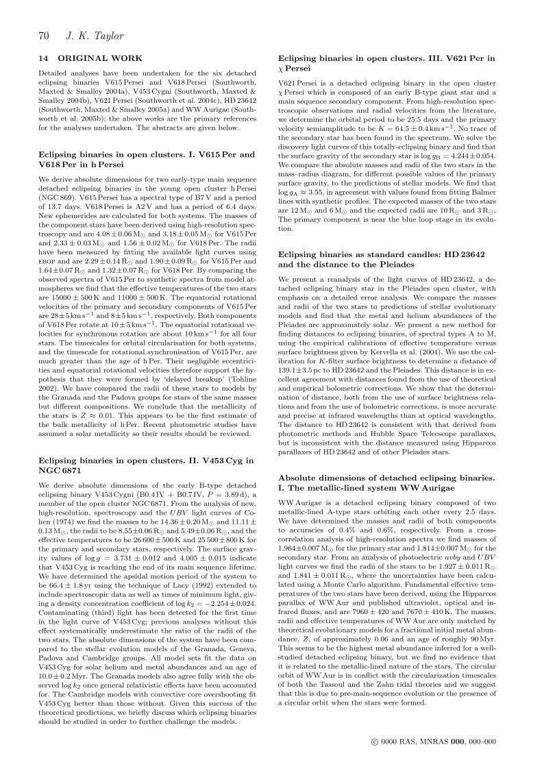
70 J. K. Taylor
14 ORIGINAL WORK
Detailed analyses have been undertaken for the six detachedeclipsing binaries V615 Persei and V618 Persei (Southworth,Maxted & Smalley 2004a), V453 Cygni (Southworth, Maxted &Smalley 2004b), V621 Persei (Southworth et al. 2004c), HD 23642(Southworth, Maxted & Smalley 2005a) and WW Aurigae (South-worth et al. 2005b); the above works are the primary referencesfor the analyses undertaken. The abstracts are given below.
Eclipsing binaries in open clusters. I. V615 Per andV618Per in hPersei
We derive absolute dimensions for two early-type main sequencedetached eclipsing binaries in the young open cluster h Persei(NGC 869). V615 Persei has a spectral type of B7 V and a periodof 13.7 days. V618 Persei is A2 V and has a period of 6.4 days.New ephemerides are calculated for both systems. The masses ofthe component stars have been derived using high-resolution spec-troscopy and are 4.08±0.06 M¯ and 3.18±0.05 M¯ for V615 Perand 2.33 ± 0.03 M¯ and 1.56 ± 0.02 M¯ for V618 Per. The radiihave been measured by fitting the available light curves usingebop and are 2.29±0.14 R¯ and 1.90±0.09 R¯ for V615 Per and1.64±0.07 R¯ and 1.32±0.07 R¯ for V618 Per. By comparing theobserved spectra of V615 Per to synthetic spectra from model at-mospheres we find that the effective temperatures of the two starsare 15000 ± 500 K and 11000 ± 500 K. The equatorial rotationalvelocities of the primary and secondary components of V615 Perare 28±5 km s−1 and 8±5 km s−1, respectively. Both componentsof V618 Per rotate at 10±5 km s−1. The equatorial rotational ve-locities for synchronous rotation are about 10 km s−1 for all fourstars. The timescales for orbital circularisation for both systems,and the timescale for rotational synchronisation of V615 Per, aremuch greater than the age of h Per. Their negligible eccentrici-ties and equatorial rotational velocities therefore support the hy-pothesis that they were formed by ‘delayed breakup’ (Tohline2002). We have compared the radii of these stars to models bythe Granada and the Padova groups for stars of the same massesbut different compositions. We conclude that the metallicity ofthe stars is Z ≈ 0.01. This appears to be the first estimate ofthe bulk metallicity of h Per. Recent photometric studies haveassumed a solar metallicity so their results should be reviewed.
Eclipsing binaries in open clusters. II. V453Cyg inNGC6871
We derive absolute dimensions of the early B-type detachedeclipsing binary V453 Cygni (B0.4 IV + B0.7 IV, P = 3.89 d), amember of the open cluster NGC 6871. From the analysis of new,high-resolution, spectroscopy and the UBV light curves of Co-hen (1974) we find the masses to be 14.36± 0.20 M¯ and 11.11±0.13 M¯, the radii to be 8.55±0.06 R¯ and 5.49±0.06 R¯, and theeffective temperatures to be 26 600±500 K and 25 500±800 K forthe primary and secondary stars, respectively. The surface grav-ity values of log g = 3.731 ± 0.012 and 4.005 ± 0.015 indicatethat V453 Cyg is reaching the end of its main sequence lifetime.We have determined the apsidal motion period of the system tobe 66.4 ± 1.8 yr using the technique of Lacy (1992) extended toinclude spectroscopic data as well as times of minimum light, giv-ing a density concentration coefficient of log k2 = −2.254±0.024.Contaminating (third) light has been detected for the first timein the light curve of V453 Cyg; previous analyses without thiseffect systematically underestimate the ratio of the radii of thetwo stars. The absolute dimensions of the system have been com-pared to the stellar evolution models of the Granada, Geneva,Padova and Cambridge groups. All model sets fit the data onV453 Cyg for solar helium and metal abundances and an age of10.0±0.2 Myr. The Granada models also agree fully with the ob-served log k2 once general relativistic effects have been accountedfor. The Cambridge models with convective core overshooting fitV453 Cyg better than those without. Given this success of thetheoretical predictions, we briefly discuss which eclipsing binariesshould be studied in order to further challenge the models.
Eclipsing binaries in open clusters. III. V621Per inχ Persei
V621 Persei is a detached eclipsing binary in the open clusterχPersei which is composed of an early B-type giant star and amain sequence secondary component. From high-resolution spec-troscopic observations and radial velocities from the literature,we determine the orbital period to be 25.5 days and the primaryvelocity semiamplitude to be K = 64.5± 0.4 km s−1. No trace ofthe secondary star has been found in the spectrum. We solve thediscovery light curves of this totally-eclipsing binary and find thatthe surface gravity of the secondary star is log gB = 4.244±0.054.We compare the absolute masses and radii of the two stars in themass–radius diagram, for different possible values of the primarysurface gravity, to the predictions of stellar models. We find thatlog gA ≈ 3.55, in agreement with values found from fitting Balmerlines with synthetic profiles. The expected masses of the two starsare 12 M¯ and 6 M¯ and the expected radii are 10 R¯ and 3 R¯.The primary component is near the blue loop stage in its evolu-tion.
Eclipsing binaries as standard candles: HD23642and the distance to the Pleiades
We present a reanalysis of the light curves of HD 23642, a de-tached eclipsing binary star in the Pleiades open cluster, withemphasis on a detailed error analysis. We compare the massesand radii of the two stars to predictions of stellar evolutionarymodels and find that the metal and helium abundances of thePleiades are approximately solar. We present a new method forfinding distances to eclipsing binaries, of spectral types A to M,using the empirical calibrations of effective temperature versussurface brightness given by Kervella et al. (2004). We use the cal-ibration for K-filter surface brightness to determine a distance of139.1±3.5 pc to HD 23642 and the Pleiades. This distance is in ex-cellent agreement with distances found from the use of theoreticaland empirical bolometric corrections. We show that the determi-nation of distance, both from the use of surface brightness rela-tions and from the use of bolometric corrections, is more accurateand precise at infrared wavelengths than at optical wavelengths.The distance to HD 23642 is consistent with that derived fromphotometric methods and Hubble Space Telecscope parallaxes,but is inconsistent with the distance measured using Hipparcosparallaxes of HD 23642 and of other Pleiades stars.
Absolute dimensions of detached eclipsing binaries.I. The metallic-lined system WW Aurigae
WW Aurigae is a detached eclipsing binary composed of twometallic-lined A-type stars orbiting each other every 2.5 days.We have determined the masses and radii of both componentsto accuracies of 0.4% and 0.6%, respectively. From a cross-correlation analysis of high-resolution spectra we find masses of1.964±0.007 M¯ for the primary star and 1.814±0.007 M¯ for thesecondary star. From an analysis of photoelectric uvby and UBVlight curves we find the radii of the stars to be 1.927± 0.011 R¯and 1.841 ± 0.011 R¯, where the uncertainties have been calcu-lated using a Monte Carlo algorithm. Fundamental effective tem-peratures of the two stars have been derived, using the Hipparcosparallax of WW Aur and published ultraviolet, optical and in-frared fluxes, and are 7960± 420 and 7670± 410 K. The masses,radii and effective temperatures of WW Aur are only matched bytheoretical evolutionary models for a fractional initial metal abun-dance, Z, of approximately 0.06 and an age of roughly 90 Myr.This seems to be the highest metal abundance inferred for a well-studied detached eclipsing binary, but we find no evidence thatit is related to the metallic-lined nature of the stars. The circularorbit of WW Aur is in conflict with the circularization timescalesof both the Tassoul and the Zahn tidal theories and we suggestthat this is due to pre-main-sequence evolution or the presence ofa circular orbit when the stars were formed.
c© 0000 RAS, MNRAS 000, 000–000
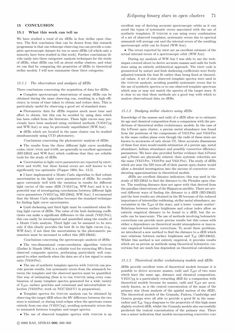
Eclipsing binary stars in open clusters 71
15 CONCLUSION
15.1 What this work can tell us
We have studied a total of six dEBs in four stellar open clus-ters. The first conclusion that can be drawn from this researchprogramme is that one telescope observing run can provide a com-plete spectroscopic dataset for ten or more dEBs (of which only aminority have been studied in this work). Further conclusions di-vide easily into three categories: analysis techniques for the studyof dEBs, what dEBs can tell us about stellar clusters, and whatwe can find by comparing the properties of dEBs to theoreticalstellar models. I will now summarise these three categories.
15.1.1 The observation and analysis of dEBs
Three conclusions concerning the acquisition of data for dEBs:
• Complete spectroscopic observations of many dEBs can beobtained during the same observing run, resulting in a high effi-ciency in terms of time taken to obtain and reduce data. This isparticularly useful for observing a good set of standard stars.
• Photometric data for dEBs requires much more time andeffort to obtain, but this can be avoided by using data whichhas been culled from the literature. These light curves may pre-viously have been analysed using outdated methods (V453 Cygand WW Aur) or may be previously unpublished (WW Aur).
• dEBs which are located in the same cluster can be studiedsimultaneously using CCD photometry.
Conclusions concerning the photometric analysis of dEBs:
• The results from the three different light curve modellingcodes, ebop, wink and wd98, are generally in excellent agreement(HD 23642 and WW Aur) which confirms that they are reliabletools for the study of dEBs.
• Uncertainties in light curve parameters are reported by ebop,wink and wd98, but these formal errors are well known to besignificantly too optimistic (Popper 1984; Sec. 13.3).
• I have implemented a Monte Carlo algorithm to find robustuncertainties in the light curve parameters of dEBs. Its resultsagree extremely well with the variation in results for differentlight curves of the same dEB (V453 Cyg, WW Aur) and it is apowerful way of investigating correlations between different lightcurve parameters (V453 Cyg, HD 23642, WW Aur). I recommendthat the Monte Carlo algorithm becomes the standard techniquefor finding light curve uncertainties.
• Limb darkening and third light must be considered when fit-ting light curves of dEBs. The value of the limb darkening coeffi-cients can make a significant difference to the result (V621 Per);this can easily be investigated and quantified using the results ofa Monte Carlo analysis. Third light can be assumed to be zeroonly if this clearly provides the best fit to the light curves (e.g.,WW Aur); if not then the uncertainties in the photometric pa-rameters must be increased to reflect this (HD 23642).
Conclusions concerning the spectroscopic analysis of dEBs:
• The two-dimensional cross-correlation algorithm todcor(Zucker & Mazeh 1994) is a reliable tool for extracting RVs fromobserved composite spectra, performing particularly well com-pared to other methods when the data are of a low signal to noiseratio (V618 Per).
• The use of synthetic template spectra with todcor can pro-vide precise results, but systematic errors from the mismatch be-tween the template and the observed spectra must be quantified.One way of estimating these is to run todcor using every com-bination of many template spectra generated for a wide varietyof Teffs, surface gravities and rotational and microturbulent ve-locities (V618 Per; work on NGC 2243 V1 in preparation).
• Template spectra for todcor analysis can be obtained byobserving the target dEB when the RV difference between the twostars is minimal, or during total eclipse when the spectrum comesentirely from one star (V453 Cyg), avoiding systematic errors dueto mismatch between template and target spectra.
• The use of observed template spectra with todcor is an
excellent way of deriving accurate spectroscopic orbits as it canavoid the types of systematic errors associated with the use ofsynthetic templates. If todcor is run using every combinationof a set of observed templates, systematic errors due to spectralmismatch will average out and the internal errors of the resultingspectroscopic orbit can be found (WW Aur).
• The errors reported by sbop are an excellent estimate of theactual internal errors of a spectroscopic orbit (WW Aur).
During my analysis of WW Aur I was able to use the tech-niques covered above to derive accurate masses and radii for bothstars using an entirely arithmetical approach. The ebop code isgeometrical by nature and limb darkening coefficients were freelyadjusted towards the best fit rather than being fixed at theoreti-cal values. A set of nine observed template spectra were used inthe todcor analysis, avoiding possible systematic errors due tothe use of synthetic spectra or to one observed template spectrumwhich may or may not match the spectra of the target stars. Itis clear to me that these methods are a good way with which toanalyse observational data on dEBs.
15.1.2 Studying stellar clusters using dEBs
Knowledge of the masses and radii of a dEB allow us to estimateits age and chemical composition from a comparison with the pre-dictions of theoretical stellar evolutionary models. In the case ofthe h Persei open cluster, a precise metal abundance was foundfrom the positions of the components of V615 Per and V618 Perin the mass–radius plane even though the radii of these stars areknown to accuracies of only about 5%. More accurate dimensionsof these four stars would enable estimation of a precise age, metalabundance, helium abundance and possibly convective efficiencyparameters. We have also provided further evidence that h Perseiand χPersei are physically related; their systemic velocities arethe same (V615 Per, V618 Per and V621 Per). The study of dEBswhich are near the MS turn-off of their parent open cluster wouldallow a detailed investigation into the success of convective over-shooting approximations in theoretical models.
dEBs are excellent distance indicators: this was used in thestudy of HD 23642 to find the distance to the Pleiades open clus-ter. The resulting distance does not agree with that derived fromthe parallax observations of the Hipparcos satellite. There are sev-eral different ways of finding the distance to a dEB (HD 23642)and the best results are obtained in the IR because of the reducedimportance of interstellar reddening, stellar metal abundance, un-certainties in the Teffs of the stars, and a lower ‘cosmic scatter’.Relations between surface brightness and colour index allow anentirely empirical distance to be found to a dEB, but the re-sults can be inaccurate. The use of methods involving bolometriccorrections can provide more precise results but this comes witheither a dependence on theoretical model atmospheres or inaccu-rate empirical bolometric corrections. To avoid these problems,we introduced a new method to find the distance to a dEB whichuses relations between surface brightness and Teff (HD 23642).Whilst this method is not entirely empirical, it provides resultswhich are as precise as methods using theoretical bolometric cor-rections but are much less dependent on theoretical calculations.
15.1.3 Theoretical stellar evolutionary models and dEBs
dEBs provide excellent tests of theoretical models because it ispossible to derive accurate masses, radii and Teffs of two starswhich have the same age, distance and chemical composition.V453 Cyg is a particularly rewarding dEB for a comparison withtheoretical models because its masses, radii and Teffs are accu-rately known, as is the central concentration of the mass of theprimary star (from analysis of the apsidal motion of the dEB).The theoretical models of the Granada, Padova, Cambridge andGeneva groups were all able to provide a good fit in the mass–radius and Teff–log g diagrams to the properties of this high-massslightly-evolved dEB, whilst the Granada models also successfullypredicted the central concentration of the primary star. Therewas a minor indication that models incorporating convective core
c© 0000 RAS, MNRAS 000, 000–000
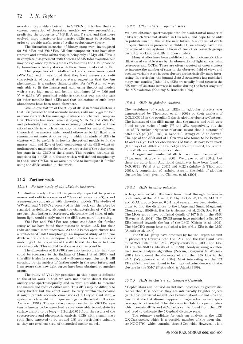
72 J. K. Taylor
overshooting provide a better fit to V453 Cyg. It is clear that thecurrent generation of theoretical models are very successful atpredicting the properties of MS B, A and F stars, and that moreevolved, more massive or less massive dEBs must be studied inorder to provide useful tests of stellar evolutionary theory.
The formation scenarios of binary stars were investigatedfor V615 Per and V618 Per. All four component stars have slowrotation and circular orbits despite being only 13 Myr old. This isin complete disagreement with theories of MS tidal evolution butmay be explained by strong tidal effects during the PMS phase orby formation of binary stars with these characteristics at birth.
The properties of metallic-lined stars were investigated(WW Aur) and it was found that they have masses and radiicharacteristic of normal A-type stars, suggesting that the Amphenomenon is a surface characteristic. For WW Aur we wereonly able to fit the masses and radii using theoretical modelswith a very high metal and helium abundance (Z = 0.06 andY = 0.36). We presented evidence that this was not the casefor other metallic-lined dEBs and that indications of such largeabundances have been noted elsewhere.
One unique feature of the study of dEBs in stellar clusters isthat it is possible to find accurate masses, radii and Teffs for fouror more stars with the same age, distance and chemical composi-tion. This was first noted when studying V615 Per and V618 Perand potentially can provide an extremely detailed test of theo-retical models in which values may be found for many differenttheoretical parameters which would otherwise be left fixed at areasonable estimate. Another way in which the study of dEBs inclusters will be useful is in forcing theoretical models to fit themasses, radii and Teffs of both components of the dEB whilst si-multaneously matching the radiative properties of the other mem-ber stars in the CMD of the cluster. This requires accurate di-mensions for a dEB in a cluster with a well-defined morphologyin the cluster CMDs, so we were not able to investigate it furtherusing the dEBs studied in this work.
15.2 Further work
15.2.1 Further study of the dEBs in this work
A definitive study of a dEB is generally expected to providemasses and radii to accuracies of 2% as well as accurate Teffs anda reasonable comparison with theoretical models. The studies ofWW Aur and V453 Cyg presented in this work can therefore beregarded as definitive, although the characteristics of V453 Cygare such that further spectroscopy, photometry and times of min-imum light would clearly make the dEB even more interesting.
V615 Per and V618 Per are prime candidates for furtherstudy as we have found their masses to within 1.5% but theirradii are much more uncertain. As the h Persei open cluster hasa well-defined CMD morphology, an improved study of the twodEBs will allow the development of tools for the simultaneousmatching of the properties of the dEBs and the cluster to theo-retical models. This should be done as soon as possible.
The dimensions of HD 23642 are also less accurate than theycould be (contrary to the findings of Munari et al. 2004) andthis dEB is also in a nearby and well-known open cluster. It willcertainly be the subject of further study in the near future, andI am aware that new light curves have been obtained by anothergroup.
The study of V621 Per presented in this paper is differentto the other work in that we were not able to detect the sec-ondary star spectroscopically and so were not able to measurethe masses and radii of either star. This dEB may be difficult tostudy further but the effort would be very worthwhile becauseit might provide accurate dimensions of a B-type giant star, asystem which would be unique amongst well-studied dEBs (seeAndersen 1991). The secondary component in the V621 Per sys-tem is known to be unevolved as we were able to calculate itssurface gravity to be log g = 4.244± 0.054 from the results of thespectroscopic and photometric analysis. dEBs with a small massratio (here expected to be around 0.5) are particularly valuableas they are excellent tests of theoretical stellar models.
15.2.2 Other dEBs in open clusters
We have obtained spectroscopic data for a substantial number ofdEBs which were not studied in this work, and hope to be ableto publish much of this in the near future. A short list of dEBsin open clusters is presented in Table 11; we already have datafor some of these systems. I know of two other research groupscurrently working on dEBs in open clusters.
Many studies have been published on the photometric iden-tification of variable stars by the observation of light curves usingtelescopes and CCDs. These are often targeted at open clustersto increase the number of stars in the observed field of view, andbecause variable stars in open clusters are intrinsically more inter-esting. In particular, the journal Acta Astronomica has publishedmany such studies (Table 11). dEBs are usually found towards theMS turn-off as stars increase in radius during the latter stages ofthe MS evolution (KaÃluzny & Rucinski 1993).
15.2.3 dEBs in globular clusters
The usefulness of studying dEBs in globular clusters wasdemonstrated by Thompson et al. (2001) by their analysis ofOGLE GC 17 in the peculiar Galactic globular cluster ωCentauri.The faintness of this dEB meant that the masses and radii werefound to accuracies of only 7% and 3%, respectively, but theuse of IR surface brightness relations meant that a distance of5360 ± 300 pc ((M −m)0 = 13.65 ± 0.12 mag) could be derived.The age of the dEB and of ωCen was also found to be between13 and 17 Gyr. Further observations of this dEB have been made(KaÃluzny et al. 2002) but have not yet been published, and severalmore dEBs are known in this cluster.
A significant number of dEBs have been discovered in47 Tucanae (Albrow et al. 2001; Weldrake et al. 2004), butthese are quite faint. Additional candidates have been found inNGC 6641 (Pritzl et al. 2001) and M 22 (KaÃluzny & Thompson2001). A compilation of variable stars in the fields of globularclusters has been given by Clement et al. (2001).
15.2.4 dEBs in other galaxies
A large number of dEBs have been found through time-seriesphotometry of the LMC and SMC by the OGLE, EROS, MACHOand MOA groups (see sec 6.3.4) and several have been studied inorder to find the distances to the LArge and Small MagellanicClouds (e.g., Hilditch, Harries & Howarth et al. 2005; Sec. 6.3.4).The MOA group have published details of 167 EBs in the SMC(Bayne et al. 2004). The EROS group have published a list of 79EBs located towards the bar of the LMC (Grison et al. 1995).The MACHO group have published a list of 611 EBs in the LMC(Alcock et al. 1997).
The OGLE group have obtained by far the largest amountof photometry towards both the LMC and the SMC and havefound 2580 EBs in the LMC (Wyrzykowski et al. 2003) and 1459EBs in the SMC (Udalski et al. 1998). Analysis using a differ-ence image analysis algorithm (Zebrun, Soszynski & Wozniak2001) has allowed the discovery of a further 455 EBs in theSMC (Wyrzykowski et al. 2004). Most interesting are the 127EBs which have been found to be in optical coincidence with starclusters in the SMC (Pietrzynski & Udalski 1999).
15.2.5 dEBs in clusters containing δ Cepheids
δCephei stars can be used as distance indicators at greater dis-tances than EBs because they are intrinsically brighter objects(with absolute visual magnitudes between about −2 and −6) andcan be studied at dimmer apparent magnitudes because spec-troscopy is not needed. The distances to Galactic open clusterswhich contain dEBs and δCepheids can be found from the dEBand used to calibrate the δCepheid distance scale.
The primary candidate for such an analysis is the dEBQX Cassiopeiae, which is a possible member of the open clus-ter NGC 7790, which contains three δCepheids. However, it is a
c© 0000 RAS, MNRAS 000, 000–000
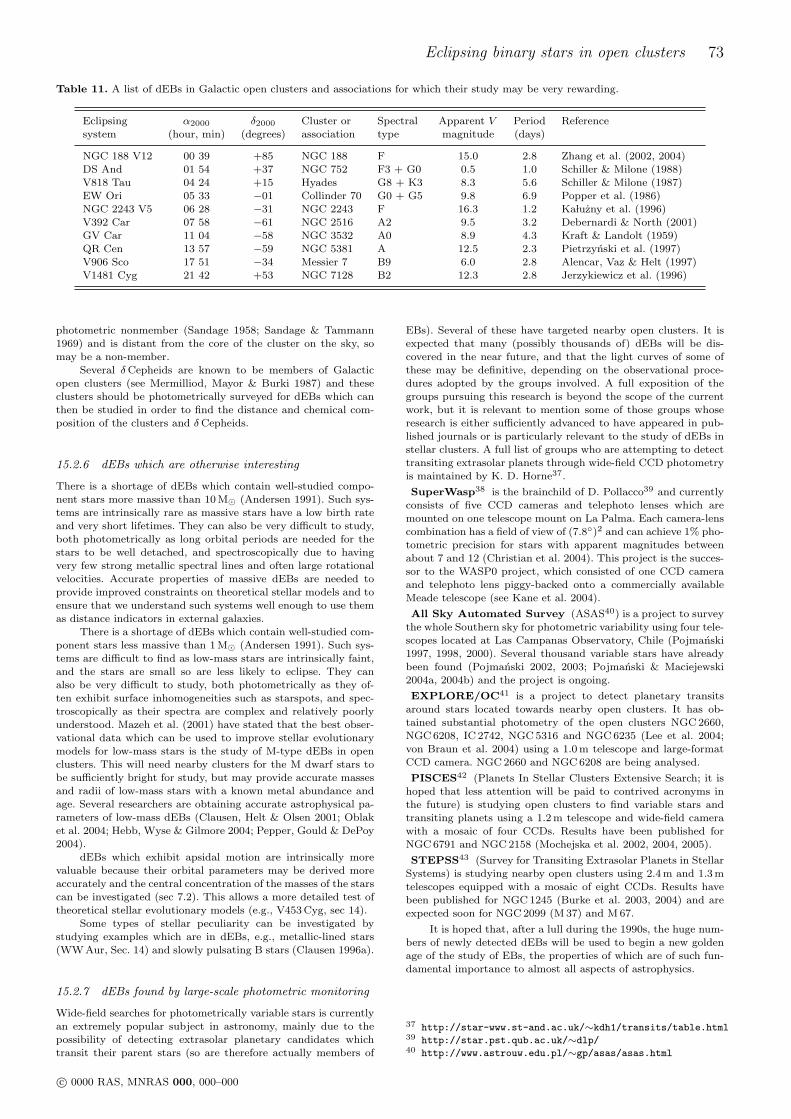
Eclipsing binary stars in open clusters 73
Table 11. A list of dEBs in Galactic open clusters and associations for which their study may be very rewarding.
Eclipsing α2000 δ2000 Cluster or Spectral Apparent V Period Referencesystem (hour, min) (degrees) association type magnitude (days)
NGC 188 V12 00 39 +85 NGC 188 F 15.0 2.8 Zhang et al. (2002, 2004)DS And 01 54 +37 NGC 752 F3 + G0 0.5 1.0 Schiller & Milone (1988)V818 Tau 04 24 +15 Hyades G8 + K3 8.3 5.6 Schiller & Milone (1987)EW Ori 05 33 −01 Collinder 70 G0 + G5 9.8 6.9 Popper et al. (1986)NGC 2243 V5 06 28 −31 NGC 2243 F 16.3 1.2 KaÃluzny et al. (1996)V392 Car 07 58 −61 NGC 2516 A2 9.5 3.2 Debernardi & North (2001)GV Car 11 04 −58 NGC 3532 A0 8.9 4.3 Kraft & Landolt (1959)QR Cen 13 57 −59 NGC 5381 A 12.5 2.3 Pietrzynski et al. (1997)V906 Sco 17 51 −34 Messier 7 B9 6.0 2.8 Alencar, Vaz & Helt (1997)V1481 Cyg 21 42 +53 NGC 7128 B2 12.3 2.8 Jerzykiewicz et al. (1996)
photometric nonmember (Sandage 1958; Sandage & Tammann1969) and is distant from the core of the cluster on the sky, somay be a non-member.
Several δCepheids are known to be members of Galacticopen clusters (see Mermilliod, Mayor & Burki 1987) and theseclusters should be photometrically surveyed for dEBs which canthen be studied in order to find the distance and chemical com-position of the clusters and δCepheids.
15.2.6 dEBs which are otherwise interesting
There is a shortage of dEBs which contain well-studied compo-nent stars more massive than 10 M¯ (Andersen 1991). Such sys-tems are intrinsically rare as massive stars have a low birth rateand very short lifetimes. They can also be very difficult to study,both photometrically as long orbital periods are needed for thestars to be well detached, and spectroscopically due to havingvery few strong metallic spectral lines and often large rotationalvelocities. Accurate properties of massive dEBs are needed toprovide improved constraints on theoretical stellar models and toensure that we understand such systems well enough to use themas distance indicators in external galaxies.
There is a shortage of dEBs which contain well-studied com-ponent stars less massive than 1 M¯ (Andersen 1991). Such sys-tems are difficult to find as low-mass stars are intrinsically faint,and the stars are small so are less likely to eclipse. They canalso be very difficult to study, both photometrically as they of-ten exhibit surface inhomogeneities such as starspots, and spec-troscopically as their spectra are complex and relatively poorlyunderstood. Mazeh et al. (2001) have stated that the best obser-vational data which can be used to improve stellar evolutionarymodels for low-mass stars is the study of M-type dEBs in openclusters. This will need nearby clusters for the M dwarf stars tobe sufficiently bright for study, but may provide accurate massesand radii of low-mass stars with a known metal abundance andage. Several researchers are obtaining accurate astrophysical pa-rameters of low-mass dEBs (Clausen, Helt & Olsen 2001; Oblaket al. 2004; Hebb, Wyse & Gilmore 2004; Pepper, Gould & DePoy2004).
dEBs which exhibit apsidal motion are intrinsically morevaluable because their orbital parameters may be derived moreaccurately and the central concentration of the masses of the starscan be investigated (sec 7.2). This allows a more detailed test oftheoretical stellar evolutionary models (e.g., V453 Cyg, sec 14).
Some types of stellar peculiarity can be investigated bystudying examples which are in dEBs, e.g., metallic-lined stars(WW Aur, Sec. 14) and slowly pulsating B stars (Clausen 1996a).
15.2.7 dEBs found by large-scale photometric monitoring
Wide-field searches for photometrically variable stars is currentlyan extremely popular subject in astronomy, mainly due to thepossibility of detecting extrasolar planetary candidates whichtransit their parent stars (so are therefore actually members of
EBs). Several of these have targeted nearby open clusters. It isexpected that many (possibly thousands of) dEBs will be dis-covered in the near future, and that the light curves of some ofthese may be definitive, depending on the observational proce-dures adopted by the groups involved. A full exposition of thegroups pursuing this research is beyond the scope of the currentwork, but it is relevant to mention some of those groups whoseresearch is either sufficiently advanced to have appeared in pub-lished journals or is particularly relevant to the study of dEBs instellar clusters. A full list of groups who are attempting to detecttransiting extrasolar planets through wide-field CCD photometryis maintained by K. D. Horne37.
SuperWasp38 is the brainchild of D. Pollacco39 and currentlyconsists of five CCD cameras and telephoto lenses which aremounted on one telescope mount on La Palma. Each camera-lenscombination has a field of view of (7.8)2 and can achieve 1% pho-tometric precision for stars with apparent magnitudes betweenabout 7 and 12 (Christian et al. 2004). This project is the succes-sor to the WASP0 project, which consisted of one CCD cameraand telephoto lens piggy-backed onto a commercially availableMeade telescope (see Kane et al. 2004).
All Sky Automated Survey (ASAS40) is a project to surveythe whole Southern sky for photometric variability using four tele-scopes located at Las Campanas Observatory, Chile (Pojmanski1997, 1998, 2000). Several thousand variable stars have alreadybeen found (Pojmanski 2002, 2003; Pojmanski & Maciejewski2004a, 2004b) and the project is ongoing.
EXPLORE/OC41 is a project to detect planetary transitsaround stars located towards nearby open clusters. It has ob-tained substantial photometry of the open clusters NGC 2660,NGC 6208, IC 2742, NGC 5316 and NGC 6235 (Lee et al. 2004;von Braun et al. 2004) using a 1.0 m telescope and large-formatCCD camera. NGC 2660 and NGC 6208 are being analysed.
PISCES42 (Planets In Stellar Clusters Extensive Search; it ishoped that less attention will be paid to contrived acronyms inthe future) is studying open clusters to find variable stars andtransiting planets using a 1.2 m telescope and wide-field camerawith a mosaic of four CCDs. Results have been published forNGC 6791 and NGC 2158 (Mochejska et al. 2002, 2004, 2005).
STEPSS43 (Survey for Transiting Extrasolar Planets in StellarSystems) is studying nearby open clusters using 2.4 m and 1.3 mtelescopes equipped with a mosaic of eight CCDs. Results havebeen published for NGC 1245 (Burke et al. 2003, 2004) and areexpected soon for NGC 2099 (M 37) and M 67.
It is hoped that, after a lull during the 1990s, the huge num-bers of newly detected dEBs will be used to begin a new goldenage of the study of EBs, the properties of which are of such fun-damental importance to almost all aspects of astrophysics.
37 http://star-www.st-and.ac.uk/∼kdh1/transits/table.html39 http://star.pst.qub.ac.uk/∼dlp/40 http://www.astrouw.edu.pl/∼gp/asas/asas.html
c© 0000 RAS, MNRAS 000, 000–000
74 J. K. Taylor
REFERENCES
Abt H. A., 1958, ApJ, 128, 139.
Abt H. A., Levato H., 1978, PASP, 90, 201.
Abt H. A., Levy S. G., 1973, ApJ, 184, 167.
Abt H. A., Morrell N. I., 1995, ApJS, 99, 135.
Abt H. A., Levy S. G., Gandet L., 1972, AJ, 77, 138.
Abt H. A., Levato H., Grosso M., 2002, ApJ, 573, 359.
Adelman S. J., Gulliver A. F., Smalley B., Pazder J. S., YoungerP. F., Boyd L., Epand D., 2004, in Zverko J., Weiss W. W.,Ziznovsky J., Adelman S. J., eds., IAU Symp. 224, The A-StarPuzzle, Cambridge Univ. Press, 911.
Albrow M. D., Gilliland R. L., Brown T. M., Edmonds P. D.,Guhathakurta P., Sarajedini A., 2001, ApJ, 559, 1060.
Alcock C., Allsman R. A., Alves D., 1997, AJ, 114, 326.
Alencar S. H. P., Vaz L. P. R., 1999, A&AS, 135, 555.
Alencar S. H. P., Vaz L. P. R., Helt B. E., 1997, A&A, 326, 709.
Allen C. W., 1973, Astrophysical Quantities (Third edition), TheAthlone Press, University of London.
Allende Prieto C., 2001, ApJ, 547, 200.
Al-Naimiy H. M. K., 1978, Ap&SS, 53, 181.
Alongi M., Bertelli G., Bressan A., Chiosi C., Fagotto F., GreggioL., Nasi E., 1993, A&AS, 97, 851.
Alonso A., Arribas S., Martınez-Roger C., 1996, A&A, 313, 873.
Alves D. R., 2004, New Astron. Rev., 48, 659.
Alves D. R., Rejkuba M., Minniti D., Cook K. H., 2002, ApJ,573, L51.
Anders E., Grevesse N., 1989, Geochimica et Cosmochimica Acta,53, 197.
Andersen J., 1975a, A&A, 44, 355.
Andersen J., 1975b, A&A, 44, 445.
Andersen J., 1975c, A&A, 45, 203.
Andersen J., 1991, A&AR, 3, 91.
Andersen J., 1993, in Weiss W. W., Baglin A., eds., ASP Conf.40., Inside the stars, 347.
Andersen J., 1998, in Bedding T. R., Booth A. J., Davis J., eds.,IAU Symp. 189, Fundamental Stellar Properties: The Inter-action between Observation and Theory, Kluwer, Dordrecht,99.
Andersen J., Clausen J. V., 1989, A&A, 213, 183.
Andersen J., Vaz L. P. R., 1984, A&A, 130, 102.
Andersen J., Vaz L. P. R., 1987, A&A, 175, 355.
Andersen J., Clausen J. V., Gimenez A., 1993, A&A, 277, 439.
Andersen J., Clausen J. V., Nordstrom B., 1980, in M. J. Plavec,D. M. Popper, R. K. Ulrich, eds., IAU Symp. 88, Close binarystars: Observations and interpretation, 81.
Andersen J., Clausen J. V., Nordstrom B., 1984, A&A, 134, 147.
Andersen J., Clausen J. V., Nordstrom B., 1990a, A&A, 228, 365.
Andersen J., Clausen J. V., Nordstrom B., 1990b, ApJ, 363, L33.
Andersen J., Clausen J. V., Nordstrom B., Reipurth B., 1981,A&A, 101, 7.
Andersen J., Clausen J. V., Jørgensen H. E., Nordstrom B., 1984,in Maeder A., Renzini A., eds., IAU Symp. 105, ObservationalTests of the Stellar Evolution Theory, 391.
Andersen J., Clausen J. V., Nordstrom B., Popper D. M., 1985,A&A, 151, 329.
Andersen J., Nordstrom B., Garcıa J. M., Gimenez A., 1987,A&A, 174, 107.
Andersen J., Clausen J. V., Nordstrom B., Gustafsson B., Van-denBerg D. A., 1988, A&A, 196, 128.
Andersen J., Clausen J. V., Nordstrom B., Tomkin J., Mayor A.,1991, A&A, 246, 99.
Argelander F., 1903, Bonner Durchmusterung des nordlichenHimmels, Eds Marcus and Weber’s Verlag, Bonn.
Arias J. I., Morrell N. I., Barba R. H., Bosch G. L., Grosso M.,Corcoran M., 2002, MNRAS, 333, 202.
Asplund M., Gustafsson B., Kiselman D., Eriksson K., 1997,A&A, 318, 521.
Asplund M., Grevesse N., Sauval A. J., 2004, in Bash F. N.,Barnes T. G.,eds., ASP Conf. Ser., Cosmic abundances asrecords of stellar evolution and nucleosynthesis, 25.
Auer L. H., Mihalas D, 1972, ApJS, 24, 193.
Bagnuolo W. G., Gies D. R., 1991, ApJ, 376, 266.
Bagnuolo W. G., Gies D. R., Wiggs M. S., 1992, ApJ, 385, 708.
Bahcall J. N., Basu S., Pinsonneault M., Serenelli A. M., 2005,ApJ, 618, 1049.
Baker R. H., 1910, Publ. Allegheny Obs., 1, 163.
Baldwin M. E., 1973, IBVS, 795.
Balog Z., Delgado A. J., Moitinho A., Furesz G., Kaszas G., VinkoJ., Alfaro E. J., 2001, MNRAS, 323, 872.
Balona L. A., 1984, MNRAS, 211, 973.
Balona L. A., 1994, MNRAS, 268, 119.
Balona L. A., Shobbrook R. R., 1984, MNRAS, 211, 375.
Baraffe I., Chabrier G., Allard F., Hauschildt P. H., 1995, ApJ,446, L35.
Barban C., Goupil M. J., Van’t Veer-Menneret C., Garrido R.,Kupka F., Heiter U., 2003, A&A, 405, 1095.
Barbosa C. l., Figer D., 2004, in press (astro-ph/0408491).
Barembaum M. J., Etzel P. B., 1995, AJ, 109, 2680.
Barnard A. J., Cooper J., Shamey L. J., 1969, A&A, 1, 28.
Barnes T. G., Evans D. S., 1976, MNRAS, 174, 489.
Barnes T. G., Evans D. S., Parsons S., 1976, MNRAS, 174, 503.
Barnes T. G., Evans D. S., Moffett T. J., 1978, MNRAS, 183,285.
Barr J. M., 1908, Journal of the Royal Astron. Soc. Canada, 2,70.
Bayne G., Tobin W., Pritchard J. D., et al., 2002, MNRAS, 331,609.
Bayne G. P., Tobin W., Pritchard J. D., Pollard K. R., AlbrowM. D., 2004, MNRAS, 349, 833.
Becker S. R., Butler K., 1988, A&AS, 76, 331.
Bellazzini M., Ferraro F. R., Pancino E., 2001, ApJ, 556, 635.
Benvenuto O. G., Serenelli A. M., Althaus L. G., Barba R. H.,Morrell N. I., 2002, MNRAS, 330, 435.
Bergbusch P. A., Vandenberg D. A., Infante L., 1991, AJ, 101,2102.
Bessell M. S., 1979, PASP, 91, 589.
Bessell M. S., 1995, PASP, 107, 672.
Bessell M. S., 2000, PASP, 112, 961.
Bessell M. S., Brett J. M., 1988, PASP, 100, 1134.
Bessell M. S., Castelli F., Plez B., 1998, A&A, 333, 231.
Bessell M. S., Castelli F., Plez B., 1998, A&A, 337, 321.
Bidelman W. P., 1943, ApJ, 98, 61.
Bikmaev I. F., Ryabchikova T. A., Bruntt H., Musaev F. A.,Mashonkina L. I., Belyakova E. V., Shimansky V. V., BarklemP. S., Galazutdinov G., 2002, A&A, 389, 537.
Binnendijk L., 1960, Properties of Double Stars, University ofPennsylvania Press, Philadelphia.
Binnendijk L., 1974, Vistas in Astronomy, 16, 61.
Binney J., Merrifield M., 1998, Galactic Astronomy, PrincetonUniversity Press.
Bıro I. B., Borkovits T., Hegedus T., Paragi Z., 1998, IBVS, 4555.
Blackwell D. E., Shallis M. J., 1977, MNRAS, 180, 177.
Blackwell D. E., Shallis M. J., Selby M. J., 1979, MNRAS, 188,847.
Blackwell D. E., Petford A. D., Shallis M. J., 1980, A&A, 82, 249.
Blackwell D. E., Petford A. D., Arribas S., Haddock D. J., SelbyM. J., 1990, A&A, 232, 396.
Boesgaard A. M., Friel E. D., 1990, ApJ, 351, 467.
Bohm-Vitense E., 1958, Zeitschrift fur Astrophysik, 46, 135.
Bohm-Vitense E., 1981, ARA&A, 19, 295.
Bonanos A. Z., Stanek K. Z., Udalski A., Wyrzykowski L., ZebrunK., Kubiak M., Szyma’nski M. K., Szewczyk O., PietrzynskiG., Soszynski I., 2004, ApJ, 611, L33.
Bonifazi A., Tosi M., Fusi Pecci F., Romeo G., 1990, MNRAS,245, 15.
Bonnell I. A., 1999, in undergraduate lecture notes, University ofSt. Andrews.
Breger M., 1988, PASP, 100, 751.
Bressan A., Fagotto F., Bertelli G., Chiosi C., 1993, A&AS, 100,647.
Broglia P., Lenouvel F., 1960, Mem. Soc. Astron. It., 30, 199.
Brown T. M., Charbonneau D., Gilliland R., Noyes R. W., Bur-rows A, 2001, ApJ, 552, 699.
Budaj J., 1996, A&A, 313, 523.
Budaj J., 1997, A&A, 326, 655.
Burgasser A. J., Kirkpatrick J. D., Brown M. E., 2002, ApJ, 564,
c© 0000 RAS, MNRAS 000, 000–000
Eclipsing binary stars in open clusters 75
421.
Burkholder V., Massey P., Morrell N., 1997, ApJ, 490, 328.
Burke C. J., DePoy D. L., Gaudi B. S., Marshall J. L., Pogge R.W., 2002, in Deming D., Seager S., eds., ASP Conf. Ser. 294,Scientific Frontiers in Research on Extrasolar Planets, 379.
Burke C. J., Gaudi B. S., DePoy D. L., Pogge R. W., PinsonneaultM. H., 2004, AJ, 127, 2382.
Burki G., Mayor M., 1986, in Earnshaw J. B., Cottrell P. L., eds.,IAU Symp. 118, Instrumentation and Research Programmesfor Small Telescopes, 385.
Butler R. P., Marcy G. W., Williams E., McCarthy C., DosanjhP., Vogt S. S., 1996, PASP, 108, 500.
Campbell W. W., 1910, Lick Obs. Bull., 6, 17.
Cannon A. J., Pickering E. C., 1918, Annals of the Astron. Obs.Harvard College, 92, 1.
Cannon A. J., Pickering E. C., 1923, Annals of the Astron. Obs.Harvard College, 98, 1.
Canterna R. W., 1976, AJ, 81, 228.
Canuto V. M., Mazzitelli I., 1991, ApJ, 370, 295.
Canuto V. M., Mazzitelli I., 1992, ApJ, 389, 724.
Capilla G., Fabregat J., 2002, A&A, 394, 479.
Carbon D. F., Gingerich O., 1969, in Gingerich O., ed., Proc.Third Harvard-Smithsonian Conference on Stellar Atmo-spheres, Cambridge, Massachusetts, 377.
Carpenter J. M., 2001, AJ, 121, 2851.
Carquillat M. J., Jaschek C., Jaschek M., Ginestet N., 1997,A&AS, 123, 5.
Carraro G., Bertelli G., Bressan A., Chiosi C., 1993, A&AS, 101,381.
Cassisi S., Castellani V., Salaris M., Straniero O., 1994, A&A,282, 760.
Castellani V., Chieffi A., Straniero O., 1992, ApJS, 78, 517.
Castellani V., Degl’Innocenti S., Prada Moroni P. G., TordiglioneV., 2002, MNRAS, 334, 193.
Castellani V., Degl’Innocenti S., Marconi M., Prada Moroni P.G., Sestito P., 2003, A&A, 404, 645.
Castelli F., Hubrig S., 2004, A&A, 425, 263.
Castelli F., Gratton R. G., Kurucz R. L., 1997, A&A, 318, 841.
Catala C., Foing B. H., Baudrand J., et al., 1993, A&A, 275, 245.
Caton D. B.; Burns W. C.; Hawkins R. L., 1991, IBVS, 3552.
Cayrel de Strobel G., Soubiran C, Ralite N, 2001, A&A, 373, 159.
Cerruti M. A., 1996, AcA, 46, 429.
Cester B., Fedel B., Giuricin G., Mardirossian F., Mezzetti M.,1978, A&AS, 33, 91.
Chaboyer B., 1995, ApJ, 444, L9.
Chaboyer B., Green E. M., Liebert J., 1999, AJ, 117, 1360.
Chabrier G., Baraffe I., 1995, ApJ, 451, L29.
Chaffee F. H., 1970, A&A, 4, 291.
Charbonnel C., Meynet, G., Maeder A., Schaerer D., 1996, A&AS,115, 339.
Charbonnel C., Dappen W., Schaerer D., Bernasconi P. A.,Maeder A., Meynet G., Mowlavi N., 1999, A&AS, 135, 405.
Chen L., Hou J., Wang J. J., 2003, AJ, 125, 1397.
Chieffi A., Straniero O., 1989, ApJS, 71, 47.
Chieffi A., Straniero O., Salaris M., 1995, ApJ, 445, L39.
Chiosi C., 1990, PASP, 102, 412.
Chiosi C., 1998, in Bedding T. R., Booth A. J., Davis J., eds., IAUSymp. 189, Fundamental Stellar Properties: The Interactionbetween Observation and Theory, Kluwer, Dordrecht, 323.
Chiosi C., Maeder A., 1986, ARA&A, 24, 329.
Chou K. C., 1959, AJ, 64, 468.
Christian D. J., Pollacco D. L., Clarkson W. L., et al., 2004, inF. Favata ed., Proceedings of the 13th Cool Stars Workshop,in press (preprint: astro-ph/0411019).
Claret A., 1995, A&AS, 109, 441.
Claret A., 1997, A&AS, 125, 439.
Claret A., 1998, A&AS, 131, 395.
Claret A., 2000a, A&A, 359, 289.
Claret A., 2000b, A&A, 363, 1081.
Claret A., 2003, A&A, 401, 657.
Claret A., 2004a, A&A, 424, 919.
Claret A., 2004b, A&A, 428, 1001.
Claret A., Cunha N. C. S., 1997, A&A, 318, 187.
Claret A., Gimenez A., 1989, A&AS, 81, 1.
Claret A., Gimenez A., 1990a, A&A, 230, 412.
Claret A., Gimenez A., 1990b, Ap&SS, 169, 223.
Claret A., Gimenez A., 1991, A&A, 244, 319.
Claret A., Gimenez A., 1992, A&AS, 96, 255.
Claret A., Gimenez A., 1993, A&A, 277, 487.
Claret A., Gimenez A., 1995, A&AS, 114, 549.
Claret A., Gimenez A., 1998, A&AS, 133, 123.
Claret A., Hauschildt P. H., 2003, A&A, 412, 241.
Claret A., Dıaz-Cordoves J., Gimenez A., 1995, A&AS, 114, 247.
Claret A., Gimenez A., Cunha N. C. S., 1995, A&A, 299, 724.
Clausen J. V., 1991, 246, 397.
Clausen J. V., 1996a, A&A, 308, 151.
Clausen J. V., 1996b, in Milone E. F., Mermilliod J.-C., eds., ASPConf. Ser. 90, The origins, evolution, and destinies of binarystars in clusters, 154.
Clausen J. V., 1998, in Kjeldsen H., Bedding T. R., eds., The FirstMONS Workshop: Science with a Small Space Telescope, 105.
Clausen J. V., 2000, in Bergeron J., Renzini A., eds., From Extra-solar Planets to Cosmology: The VLT Opening Symposium,225.
Clausen J. V., 2004, New Astron. Rev., 48, 679.
Clausen J. V., Gimenez A., 1987, in J. Palous, ed., 10th EuropeanRegional Astronomy Meeting of the IAU, Prague, 185.
Clausen J. V., Gimenez A., 1991, A&A, 241, 98.
Clausen J. V., Gimenez A., Scarfe C., 1986, A&A, 167, 287.
Clausen J. V., Gimenez A., van Houten C. J., 1995, A&AS, 109,425.
Clausen J. V., Helt B. E., Olsen E. H., 2001, A&A, 374, 980.
Clausen J. V., Helt B. E., Olsen E. H., Garcıa J. M., 1998, inBedding T. R., Booth A. J., Davis J., eds., IAU Symp. 189,Fundamental Stellar Properties: The Interaction between Ob-servation and Theory, Kluwer, Dordrecht, poster proceedingsp. 56.
Clausen J. V., Baraffe I., Claret A., Vandenberg D. A., 1999, in A.Gimenez, E. F. Guinan & B. Montesinos, eds., ASP Conf. Ser.173, Stellar Structure: Theory and Test of Connective EnergyTransport, 265.
Clausen J. V., Storm J., Larsen S. S., Gimenez A., 2003, A&A,402, 509.
Clement C. M., Muzzin A., Dufton Q., et al., 2001, AJ, 122, 2587.
Clementini G., Gratton R., Bragaglia A., Carretta E., Di FabrizioL., Maio M., 2003, AJ, 125, 1309.
Code A. D., Bless R. C., Davis J., Brown R. H., 1976, ApJ, 203,417.
Cohen H. L., 1969, AJ, 74, 1168.
Cohen H. L., 1971, PASP, 83, 677.
Cohen H. L., 1974, A&AS, 15, 181.
Colavita M., Akeson R., Wizinowich P., et al. 2003, ApJ, 592,L83.
Collins G. W., Truax R. J., 1995, ApJ, 439, 860.
Cordier D., Lebreton Y., Goupil M.-J., Lejeune T., Beaulieu J.-P.,Arenou F., 2002, A&A, 392, 169.
Cousins A. W. J., 1980, SAAO Circular, 1, 234.
Cowley C. R., 1995, An Introduction to Cosmochemistry, Cam-bridge University Press.
Cox A. N., Stewart J. N., 1962, AJ, 67, 113.
Cox A. N., Stewart J. N., 1965, ApJS, 11, 22.
Cox A. N., Stewart J. N., 1970a, ApJS, 19, 243.
Cox A. N., Stewart J. N., 1970b, ApJS, 19, 261.
Cox A. N., Tabor J. E., 1976, ApJS, 31, 271.
Cox A. N., 2000, Allen’s Astrophysical Quantities (Fourth Edi-tion), AIP Press, New York.
Crawford D. L., 1958, ApJ, 128, 185.
Crawford D. L., 1975, AJ, 80, 955.
Crawford D. L., 1978, AJ, 83, 48.
Crawford D. L., 1979, AJ, 84, 1858.
Crawford D. L., 1980, AJ, 85, 621.
Crawford D. L., 1994, Rev. Mex. Astron. Astroph., 29, 115.
Crawford D. L., Barnes J. V., 1970, 75, 987.
Crawford D. L., Mander J. V., 1966, AJ, 71, 114.
Crawford D. L., Mandwewala N., 1976, PASP, 88, 917.
Crawford D. L., Perry C. L., 1976, AJ, 81, 419.
c© 0000 RAS, MNRAS 000, 000–000
76 J. K. Taylor
Crawford D. L., Barnes J. V., Warren W. H., 1974, AJ, 79, 623.
Crawford D. L., Glaspey J. W., Perry C. L., 1970, AJ, 75, 822.
Crawford D. L., Barnes J. V., Gibson J., Golson J. C., Perry C.L., Crawford M. L., 1972, A&AS, 5, 109.
Crinklaw G., Etzel P. B., 1989, AJ, 98, 1418.
Daflon S., Cunha K., Butler K., Smith V. V., 2001, ApJ, 563,325.
D’Antona F., Mazzitelli I, 1994, ApJS, 90, 467.
Dall’Ora M., Storm J., Bono G., et al., 2004, ApJ, 610, 269.
Daniel S. A., Latham D. W., Mathieu R. D., Twarog B. A., 1994,PASP, 106, 281.
Davis J., Tango W. J., Booth A. J., 2000, MNRAS, 318, 387.
Davis J., Tango W. J., Booth A. J., Ten Brummelaar T. A., Mi-nard R. A., Owens S. M., 1999a, MNRAS, 303, 773.
Davis J., Tango W. J., Booth A. J., Thorvaldson E. D., GiovannisJ., 1999b, MNRAS, 303, 783.
de Zeeuw P. T., Hoogerwerf R., de Bruijne J. H. J., Brown A. G.A., Blaauw A., 1999, AJ, 117, 354.
Debernardi Y., North P., 2001, A&A, 374, 204.
Demarque P., Woo J.-H., Kim Y.-C., Yi S. K., 2004, ApJS, 155,667.
di Benedetto G. P., 1993, A&A, 270, 315.
di Benedetto G. P., 1998, A&A, 339, 858.
Di Folco E., Thevenin F., Kervella P., Domiciano de Souza A.,Coude du Foresto V., Segransan D., Morel P., 2004, A&A,426, 601.
Dias W. S., Alessi B. S., Moitinho A., Lepine J. R. D., 2002,A&A, 389, 871.
Dıaz-Cordoves J., Gimenez A., 1992, A&A, 259, 227.
Dıaz-Cordoves J., Claret A., Gimenez A., 1995, A&AS, 110, 329.
Dinescu D. I., Girard T. M., van Altena W. F., Yang T.-G., LeeY.-W., 1996, AJ, 111, 1205.
Draper P. W., Gray N., Berry D. S., 2004, Software User NoteSUN/214.15, Starlink.
Dravins D., Lindegren L., Madsen S., 1999, A&A, 348, 1040.
Drechsel H., Haas S., Lorenz R., Gayler S., 1995, A&A, 294, 723.
Ducati J. R., Ribeiro D., Rembold S. B., 2003, ApJ, 588, 344.
Dufton P. L., Brown P. J. F., Fitzsimmons A., Lennon D. J., 1990,A&A, 232, 431.
Dugan T. S., 1930, Contributions from the Princeton UniversityObservatory, 10.
Duquennoy A., Mayor M., 1991, A&A, 248, 485.
Duquennoy A., Mayor M., Halbwachs J.-L., 1991, A&AS, 88, 281.
Dworetsky M. M, Moon T. T., 1986, MNRAS, 220, 787.
Eaton J. A., Poe C. H., 1984, AcA, 34, 97.
Eaton N., Draper P. W., Allen A., 1999, Software User NoteSUN/45.9, Starlink.
Ebersberger J., Pohl E., Kizilirmak A., 1978, IBVS, 1449.
Edvardsson B., Andersen J., Gustafsson B., Lambert D. L., NissenP. E., Tomkin J., 1993, A&A, 275, 101.
Eggen O. J., 1965, AJ, 70, 19.
Eggleton P. P., 1971, MNRAS, 151, 351.
Eggleton P. P., 1972, MNRAS, 156, 361.
Eggleton P. P., Faulkner J., Flannery B. P., 1973, A&A, 23, 325.
Eisberg R., Resnick R., 1985, Quantum Physics of Atoms,Molecules, Solids, Nuclei and Particles (Second Edition), JohnWiley & Sons, USA.
Elias J. H., Frogel J. A., Matthews K., Neugebauer G., 1982, AJ,87, 1029.
Etzel P. B., 1975, Masters Thesis, San Diego State University.
Etzel P. B., 1980, ebop Users Guide (San Diego State University.
Etzel P. B., 1981, Photometric and Spectroscopic Binary Systems,NATO ASI, 111.
Etzel P. B., 1993, in Milone E. F., ed., Light Curve Modelling ofEclipsing Binary Stars, Springer-Verlag, 113.
Etzel P. B., 2004, sbop: Spectroscopic Binary Orbit Program, SanDiego State Univ.
Fagotto F., Bressan A., Bertelli G., Chiosi C., 1994a, A&AS, 104,365.
Fagotto F., Bressan A., Bertelli G., Chiosi C., 1994b, A&AS, 105,29.
Fagotto F., Bressan A., Bertelli G., Chiosi C., 1994c, A&AS, 105,39.
Feast M. W., 2003, Lecture Notes in Physics, 635, 45 (preprint:astro-ph/0301100).
Ferluga S., Floreano L., Bravar U., Bedalo C., 1997, A&AS, 121,201.
Fernandes J., Lebreton Y., Baglin A., Morel P., 1998, A&A, 338,455.
Fitch W. S., 1964, AJ, 69, 316.
Fitzpatrick E. L., 1999, PASP, 111, 63.
Fitzpatrick E. L., Massa D., 1986, ApJ, 307, 286.
Fitzpatrick E. L., Massa D., 1988, ApJ, 328, 734.
Fitzpatrick E. L., Massa D., 1990, ApJS, 72, 163.
Fitzpatrick E. L., Massa D., 1999, ApJ, 525, 1011.
Fitzpatrick E. L., Ribas I., Guinan E. F., DeWarf L. E., MaloneyF. P., Massa D., 2002, ApJ, 564, 260.
Fitzpatrick E. L., Ribas I., Guinan E. F., Maloney F. P., ClaretA., 2003, ApJ, 587, 685.
Flower P. J., 1996, ApJ, 469, 355.
Fremat Y., Lampens P., Hensberge H., 2005, MNRAS, 356, 545.
Ford E. B., 2005, AJ, 129, 1706.
Freedman W. L., Madore B. F., Gibson B. K., et al., 2001, ApJ,553, 47.
Friel E. D., 1995, ARA&A, 33, 381.
Fukugita M., Ichikawa T., Gunn J. E., Doi M., Shimasaku K.,Schneider D. P., 1996, AJ, 111, 1748.
Gal-Yam A., Maoz D., 2004, MNRAS, 347, 942.
Gaposchkin S., 1962, AJ, 67, 358.
Gaposchkin S., 1970, IBVS, 496.
Garmany C. D., Stencel R. E., 1992, A&AS, 94, 211.
Gatewood G., de Jonge J. K., Han I., 2000, ApJ, 533, 938.
Gieren W. P., Barnes T. G., Moffett T. J., 1993, ApJ, 418, 135.
Gies D. R., Lambert D. L., 1992, ApJ, 387, 673.
Gimenez A., 1985, ApJ, 297, 405.
Gimenez A., 1992, in Kondo Y., Sistero R. F., Polidan R. S., eds.,IAU Symp. 151, Evolutionary Processes in Interacting BinaryStars, 31.
Gimenez A., Claret A., 1992, in Kondo Y., Sistero R. F., Pol-idan R. S., eds., IAU Symp. 151, Evolutionary Processes inInteracting Binary Stars, 277.
Gimenez A., Clausen J. V., 1994, A&A, 291, 795.
Gimenez A., Clausen J. V., 1996, in Milone E. F., MermilliodJ.-C., eds., ASP Conf. Ser. 90, The origins, evolution, anddestinies of binary stars in clusters, 44.
Gimenez A., Garcia-Pelayo J. M., 1983, Ap&SS, 92, 203.
Gimenez A., Quintana J. M., 1992, A&A, 260, 227.
Gimenez A., Scaltriri F., 1982, A&A, 115, 321.
Girardi L., Bressan A., Chiosi C., Bertelli G., Nasi E., 1996,A&AS, 117, 113.
Girardi L, Groenewegen M. A. T., Weiss A., Salaris M., 1998,MNRAS, 301, 149.
Girardi L., Bressan A., Bertelli G., Chiosi C., 2000, A&AS, 141,371.
Girardi L., Bertelli G., Bressan A., Chiosi C., Groenewegen M. A.T., Marigo P., Salasnich B., Weiss A., 2002, A&A, 391, 195.
Girardi L., Grebel E. K., Odenkirchen M., Chiosi C., 2004, A&A,422, 205.
Giuricin G., Mardirossian F., Mezzetti M., 1984a, A&A, 131, 152.
Giuricin G., Mardirossian F., Mezzetti M., 1984b, A&A, 134, 365.
Giuricin G., Mardirossian F., Mezzetti M., 1984c, A&A, 135, 393.
Giuricin G., Mardirossian F., Mezzetti M., 1984d, A&A, 141, 227.
Giuricin G., Mardirossian F., Mezzetti M., 1985, A&AS, 59, 37.
Glass I. S., 1973, MNRAS, 164, 155.
Goldman I., Mazeh T., 1991, ApJ, 376, 260.
Goldreich P., Nicholson P. D., 1989, ApJ, 342, 1079.
Golay M., 1966, in Loden K., Loden L. O., Sinnerstand U., eds.,IAU Symp. 24, Spectral Classification and Multicolour Pho-tometry, 262
Gonzalez J. F., Lapasset E., 2002, AJ, 123, 3318.
Graczyk D., 2003, MNRAS, 342, 1334.
Gray D. F., 1992, The Observation and Analysis of Stellar Pho-tospheres (Second Edition), Cambridge University Press.
Gray D. F., Toner C. G., 1985, PASP, 97, 543.
Gray R. O., Napier M. G., Winkler L. I., 2001, AJ, 121, 2148.
Grevesse N., Noels A, Sauval A. J., 1996, in Holt S. S., Sonneborn
c© 0000 RAS, MNRAS 000, 000–000
Eclipsing binary stars in open clusters 77
G.,eds., ASP Conf. Ser. 99, Cosmic Abundances, 117.
Griffin R. F., 1967, ApJ, 148, 465.
Griffin R. F., 2001, The Observatory, 121, 315.
Griffin R. F., 2003, The Observatory, 123, 203.
Griffin R. F., 2004, The Observatory, 124, 97.
Griffin R. F., Emerson B., 1975, The Observatory, 95, 23.
Griffin R. F., Carquillat J.-M., Ginestet N., 2003, The Observa-tory, 123, 69.
Griffin R. F., Griffin R. E. M., Gunn J. E., Zimmerman B. A.,1985, AJ, 90, 609.
Grison P., Beaulieu J.-P., Pritchard J. D., 1995, A&AS, 109, 447.
Groenewegen M. A. T., Salaris M., 2001, A&A, 366, 752.
Groenewegen M. A. T., Salaris M., 2003, A&A, 410, 887.
Groenewegen M. A. T., 2004, MNRAS, 353, 903.
Grygar J., 1965, Bull. Astron. Inst. Czechoslovakia, 16, 195.
Gudur N., 1978, Ap&SS, 57, 17.
Guinan E. F., 2004, New Astron. Rev., 48, 647.
Guinan E. F., Fitzpatrick E. L., DeWarf L. E., et al., 1998, ApJ,509, L21.
Gustafsson B., Bell R. A., Eriksson K., Nordlund A., 1975, A&A,42, 407.
Habets G. M. H. J., Heintze J. R. W., 1981, A&AS, 46, 193.
Hadrava P., 1990, Contr. Astron. Obs. Skalnate Pleso, 20, 23.
Hadrava P., 1995, A&AS, 114, 393.
Hanbury Brown R., Davis J., Allen L. R., 1967, MNRAS, 137,375.
Hanbury Brown R., Davis J., Allen L. R., 1974, MNRAS, 167,121.
Hanbury Brown R., Davis J., Allen L. R., Rome J. M., 1967,MNRAS, 137, 393.
Hanbury Brown R., Davis J., Lake R. J. W., Thompson R. J.,1974, MNRAS, 167, 475.
Harmanec P., 1988, Bull. Astron. Inst. Czechoslovakia, 39, 329.
Harries T. J., Hilditch R. W., Howarth I. D., 2003, MNRAS, 339,157.
Hauck B., Mermilliod M., 1998, A&AS, 129, 431.
Haywood M., 2002, MNRAS, 337, 151.
Hebb L., Wyse R. F. G., Gilmore G., 2004, AJ, 128, 2881.
Hejlesen P. M., 1980a, A&A, 84, 135.
Hejlesen P. M., 1980, A&AS, 39, 347.
Hejlesen P. M., 1987, A&AS, 69, 251.
Hensberge H., Pavlovski K., Verschueren V., 2000, A&A, 358,553.
Herrero A., Puls J., Najarro F., 2002, A&A, 396, 949.
Herrero A., Puls J., Villamariz M. R., 2000, A&A, 354, 193.
Herrero A., Kudritzki R. P., Vilchez J. M., Kunze D., Butler K.,Haser S., 1992, A&A, 261, 209.
Heyrovsky D., 2003, ApJ, 594, 464.
Hidas M. G., Ashley M. C. B., Webb J. K., et al., 2005, MNRAS,360, 703.
Hilditch R. W., 1973, MNRAS, 164, 101.
Hilditch R. W., 1997, in undergraduate lecture notes, Universityof St. Andrews.
Hilditch R. W., 2001, An Introduction to Close Binary Stars,Cambridge University Press.
Hilditch R. W., 2004, in Hilditch R. W., Hensberge H., PavlovskiK., eds., ASP Conf. Ser. 318, Spectroscopically and SpatiallyResolving the Components of Close Binary Stars, 318.
Hilditch R. W., Harries T. J., Howarth I. D., 2004, New Astron.Rev., 48, 687.
Hilditch R. W., Harries T. J., Howarth I. D., 2005, MNRAS, 357,304.
Hill G., 1979, Pub. Dominion Astroph. Obs. Victoria, 15, 322.
Hill G., Hutchings J. B., 1970, ApJ, 162, 265.
Hillier D. J., Miller D. L., 1998, ApJ, 496, 407.
Høg E., Kuzmin A., Bastian U., Fabricius C., Kuimov K., Linde-gren L., Makarov V. V., Roser S., 1998, A&A, 335, L65.
Høg E., Fabricius C., Makarov V. V., et al., 2000, A&A, 355, L27.
Hoag A. A., Johnson H. L., Iriarte B., Mitchell R. I., Hallam K.L., Sharpless S., 1961, Publ. U. S. Naval Obs., 17, 450.
Holmgren D., Wolf M., 1996, Obs, 116, 307.
Holmgren D. E., Scarfe C. D., Hill G., Fisher W., 1990, A&A,231, 89.
Horne K., 1986, PASP, 98, 609.
Howarth I. D., 1993, The Observatory, 113, 75.
Howarth I. D., Siebert K. W., Hussain G. A., Prinja R. K., 1997,MNRAS, 284, 265.
Hron J., 1987, A&A, 176, 34.
Huebner W. F., Merts A. L., Magee N. H., Argo M. F., 1977, LosAlamos Scientific Laboratory Report, LA-6760-M.
Huffer C. M., Kopal Z., 1951, ApJ, 114, 297.
Humphreys R. M., 1978, ApJS, 38, 309.
Hurley J. R., Pols O. R., Tout C. A., 2000, MNRAS, 315, 543.
Hurley J. R., Tout C. A., Pols O. R., 2002, MNRAS, 329, 897.
Hut P., 1981, A&A, 99, 126.
Hutsemekers D., 1993, ApJ, 417, 97.
Hynes R. I., Maxted P. F. L., 1998, A&A, 331, 167.
Iglesias C. A., Rogers F. J., 1991, ApJ, 371, 408.
Ilijic S., 2003, MSc. Thesis, University of Zagreb.
Irwin J. B., 1947, ApJ, 106, 380.
Ivanova N., Belczynski K., Fregeau J. M., Rasio F. A., 2005, MN-RAS, 358, 572.
Ivezic, Z., Lupton R. H., Anderson S., et al., 2003, Mem. Soc.Astron. It., 74, 978.
Jacoby G. H., Hunter D. A., Christian C. A., 1984, ApJS, 56, 257.
Jensen K. S., Clausen J. V., Gimenez A., 1988, A&AS, 74, 331.
Jeffries R. D., Thurston M. R., Hambly N. C., 2001, A&A, 375,863.
Jerzykiewicz M., Pigulski A., Kopacki G., MiaÃlkowska A., Niczy-poruk S., 1996, AcA, 46, 253.
Johnson H. L., 1957, ApJ, 126, 121.
Johnson H. L., 1958, Lowell. Obs. Bull., 4, 37.
Johnson H. L., 1965, ApJ, 141, 923.
Johnson H. L., 1966, ARA&A, 4, 193.
Johnson H. L., Mitchell R. I., 1958, ApJ, 128, 31.
Johnson H. L., Morgan W. W., 1953, ApJ, 117, 313.
Jones T. J., Hyland A R., 1982, MNRAS, 200, 509.
Joy A. H., 1918, PASP, 30, 253.
Kallrath J., Linnell A. P., 1987, ApJ, 313, 364.
Kallrath J., Milone E. F., Terrell D., Young, A. T., 1998, ApJ,508, 308.
KaÃluzny J., Rucinski S. M., 1993, MNRAS, 265, 34.
KaÃluzny J., Rucinski S. M., 1995, A&AS, 114, 1.
KaÃluzny J., Thompson I. B., 2001, A&A, 373, 899.
KaÃluzny J., Thompson I. B., 2003, AJ, 125, 2534.
KaÃluzny J., Udalski A., 1992, AcA, 42, 9.
KaÃluzny J., Krzeminski W., Mazur B., 1996, A&AS, 118, 303.
KaÃluzny J., Stanek K. Z., Krockenberger M., Sasselov D. D.,Tonry J. L., Mateo M., 1998, AJ, 115, 1016.
KaÃluzny J., Mochejska B. J., Stanek K. Z., Krockenberger M.,Sasselov D. D., Tonry J. L., Mateo M., 1999, AJ, 118, 346.
KaÃluzny J., Thompson W., Krzeminski A., Olech W., Pych B.,Mochejska B., 2002, in F. van Leeuwen, J. D. Hughes and G.Piotto, eds., ASP Conf. Proc. 265, Omega Centauri, A UniqueWindow into Astrophysics, 155.
Kane S. R., Collier Cameron A., Horne K. D., James D., Lister T.A., Pollacco D. L., Street R. A., Tsapras Y., 2004, MNRAS,353, 689.
Katz D., Munari U., Cropper M., 2004, MNRAS, 354, 1223.
Kaufmann W. J., 1994, Universe (Fourth Edition), W. H. Free-man and Company.
Keller S. C., Wood P. R., 2002, ApJ, 578, 144.
Keller S. C., Grebel E. K., Miller G. J., Yoss K. M., 2001, AJ,122, 248.
Kervella P., Thevenin F., Morel P., Borde P., Di Folco E., 2003,A&A, 408, 681.
Kervella P., Thevenin F., Morel P., Berthomieu G., Borde P.,Provost J., 2004a, A&A, 413, 251.
Kervella P., Nardetto N., Bersier D., Mourard D., Coude duForesto V., 2004b, A&A, 416, 941.
Kervella P., Bersier D., Mourard D., Nardetto N., Coude duForesto V., 2004c, A&A, 423, 327.
Kervella P., Thevenin F., Di Folco E., Segransan D., 2004, A&A,426, 297.
Khaliullin Kh. F., 1985, ApJ, 299, 668.
Kharitonov A. V., Tereshchenko V. M., Knjazeva L. N., 1988,
c© 0000 RAS, MNRAS 000, 000–000

78 J. K. Taylor
Alma-Ata, Nauka, 484 (CDS catalogue: III/202).
Khopolov P. N., Samus N. N., Frolov M. S., et al., 1999, VizieROn-line Data Catalogue II/214A.
Kilian J., Montenbruck O., Nissen P. E., 1991, A&AS, 88, 101.
Kilkenny D., O’Donoghue D., Koen C., Lynas-Gray A. E., vanWyk F., 1998, MNRAS, 296, 329.
Kim C., 1990, Ap&SS, 168, 153.
Kippenhahn R., Weigert A., Hofmeister E., 1967, in Methods inComputational Physics, Vol. 7 (Academic Press, New York),129.
Kirkpatrick J. D., Reid I. N., Liebert J., et al., 1999, ApJ, 519,802.
Kiss L. L., Szabo Gy. M., Sziladi K., Furesz G., Sarneczky K.,Csak B., 2001, A&A, 376, 561.
Kitamura M., 1967, Tables of the characteristic functions of theeclipse and the related delta-functions for solution of lightcurves of eclipsing binary systems, University of Tokyo Press,Tokyo.
Kitamura M., Kondo M., 1978, Ap&SS, 56, 341.
Kitamura M., Kim T.-H., Kiyokawa M., 1976, Ann. Tokyo Astron.Obs., 16, 22.
Kiyokawa M., Kitamura M.,1975, Ann. Tokyo Astron. Obs., 15,117.
Kizilirmak A., Pohl E., 1974, IBVS, 937.
Kleinmann S. G., Lysaght M. G., Pughe W. L., et al., 1994,Ap&SS, 217, 11.
Klinglesmith D. A., Sobieski S., 1970, AJ, 75, 175.
Koch R. H., Hrivnak B. J., 1981, AJ, 86, 438.
Kochukhov O., Khan S., Shulyak D., 2005, A&A, 433, 671.
Koestler A., 1989, The Sleepwalkers, Penguin Books, UK.
Kopal Z., 1939, ApJ, 90, 289.
Kopal Z., 1946, Harvard Obs. Monograph No. 6, Harvard CollegeObservatory.
Kopal Z., 1950, Harvard Obs. Monograph No. 8, Harvard CollegeObservatory.
Kopal Z., 1959, Close Binary Systems, Chapman & Hall, London.
Kraft R. P., Landolt A. U., 1959, ApJ, 129, 287.
Kristenson H., 1966, Bull. Astron. Inst. Czechoslovakia, 17, 123.
Kron G. E., 1952, ApJ, 115, 301.
Kron G. E., Smith J. L., 1951, ApJ, 113, 324.
Kruszewski A., Semeniuk I., 1999, AcA, 49, 561.
Krzesinski J., Pigulski A., 1997, A&A, 325, 987 (KP97).
Krzesinski J., Pigulski A., KoÃlaczkowski Z., 1999, A&A, 345, 505(KPK99).
Kubat J., Korcakova D., 2004, in Zverko J., Weiss W. W.,Ziznovsky J., Adelman S. J., eds., IAU Symp. 224, The A-Star Puzzle, Cambridge Univ. Press, 13.
Kudritzki R. P., 1975, Astron. Gesellschaft, 36, 81.
Kudritzki R. P., 1976, A&A, 52, 11.
Kudritzki R. P., Hummer D. G., 1990, ARA&A, 28, 303.
Kunzli M., North P., Kurucz R. L., Nicolet B., 1997, A&AS, 122,51.
Kupka F., 1996, in Adelman S. J., Kupka F., Weiss W. W., ASPConf. Ser. 108, Model Atmospheres and Spectrum Synthesis,73.
Kurucz R. L., 1975, in Philip A. G. D., Hayes D. S., eds., Multi-colour Photometry and the Theoretical HR Diagram, DudleyObs. Rep., 9, 271.
Kurucz R. L., 1979, ApJS, 40, 1.
Kurucz R. L., 1993a, in Milone E. F., ed., Light Curve Modellingof Eclipsing Binary Stars, Springer-Verlag, 93.
Kurucz R. L., 1993b, CD-ROM 13, SAO.
Kurucz R. L., 1998, in Bedding T. R., Booth A. J., Davis J., eds.,IAU Symp. 189, Fundamental Stellar Properties: The Inter-action between Observation and Theory, Kluwer, Dordrecht,217.
Kurucz R. L., 2002c, in Chavez M., Bressan A., Buzzoni A.,Mayya D., New quests in stellar astrophysics: the link betweenstars and cosmology, 3.
Kurucz R. L., 2002a, in Schultz D. R., Predrag S. K., OwnbyF., in AIP Conf. Proc. 636, Atomic and Molecular Data andTheir Applications, 134.
Kurucz R. L., 2002b, Baltic Astron., 11, 101.
Kurucz R. L., 2003, in Piskunov N., Weiss W. W., Gray D. F.,eds., IAU. Symp. 210, Modelling of Stellar Atmospheres, 45.
Kurucz R. L., Bell B., 1995, CD-ROM 23, SAO.
Kwee K. K., van Woerden H., 1956, Bull. Ast. Inst. Netherlands,12, 327.
Lacy C. H., 1977a, ApJ, 213, 458.
Lacy C. H., 1977b, ApJ, 218, 444.
Lacy C. H., 1977c, ApJS, 34, 479.
Lacy C. H., 1978, ApJ, 228, 138.
Lacy C. H., 1979, ApJ, 28, 817.
Lacy C. H., 1982, ApJ, 261, 612.
Lacy C. H., Frueh M. L., Turner A. E., 1987, AJ, 94, 1035.
Lacy C. H. S., 1992, AJ, 104, 2213.
Lacy C. H. S., Claret A., Sabby J. A., 2004, AJ, 128, 1340.
Lacy C. H. S., Torres G., Claret A., Sabby J. A., 2002, AJ, 123,1013.
Lacy C. H. S., Torres G., Claret A., Sabby J. A., 2003, AJ, 126,1905.
Lacy C. H. S., Vaz L. P. R., Claret A., Sabby J. A., 2004, AJ,128, 1324.
Landolt A. U., 1983, AJ, 88, 439.
Landolt A. U., 1992, AJ, 104, 340.
Lane B. F., Colavita M. M., 2003, AJ, 125, 1623.
Lastennet E., Valls-Gabaud D., 2002, A&A, 396, 551.
Lastennet E., Fernandes J., Lejeune Th., 2002, A&A, 388, 309.
Lastennet E., Valls-Gabaud D., Oblak E., 2000, in Reipurth B.,Zinnecker H., eds., IAU Symp. 200, Birth and Evolution ofBinary Stars, 164.
Lastennet E., Fernandes J., Valls-Gabaud D., Oblak E., 2003,A&A, 409, 611.
Latham D. W., Mazeh T., Stefanik R. P., Davis R. J., CarneyB. W., Krymolowski Y., Laird J. B., Torres G., Morse J. A.,1992, AJ, 104, 774.
Latham D. W., Nordstrom B., Andersen J., Torres G., StefanikR. P., Thaller M., Bester M. J., 1996, A&A, 314, 864.
Lavrov M. I., 1993, Tr. Kazansk. Gor. Astron. Obs., 53, 34.
Lebovitz N. R., 1974, ApJ, 190, 121.
Lebovitz N. R., 1984, ApJ, 284, 364.
Lebreton Y., 2000, ARA&A, 38, 35.
Lebreton Y., Fernandes J., Lejeune T., 2001, A&A, 374, 540.
Lee B. L., von Braun K., Mallen-Ornelas G., Yee H. K. C., SeagerS., Gladders M. D., 2004, in Holt S. S., Deming D., eds., AIPConf. Proc. 713, The Search for Other Worlds, 177.
Lee E. B., 1997, AJ, 113, 1106.
Leggett S. K., Allard F., Burgasser A. J., Jones H. R. A., MarleyM. S., Tsuji T., 2004, Proc. 13th Cool Stars Workshop, inpress (preprint astro-ph/0409389).
Lennon D. J., Brown P. J. F., Dufton P. L., 1988, A&A, 195, 208.
Leung K.-C., Schneider D. P., 1978, AJ, 83, 618.
Leung K.-C., Wilson R. E., 1977, ApJ, 211, 853.
Levato H., Morrell N., 1983, Astroph. Lett., 23, 183.
Levenberg K., 1944, Q. Appl. Math., 2, 164.
Lindegren L., Perryman M. A. C., 1996, A&AS, 116, 579.
Linnell A. P., 1984, ApJS, 54, 17.
Linnell A. P., 1986, ApJ, 300, 304.
Lindegren L., Dravins D., 2003, A&A, 401, 1185.
Littlefair S. P., Naylor T, Jeffries R. D., Devey C. R., Vine S.,2003, MNRAS, 345, 1205.
Liu T., Janes K. A., Bania T. M., 1989, AJ, 98, 626.
Liu T., Janes K. A., Bania T. M., 1991, AJ, 102, 1103.
Lorenz R., Mayer P., Drechsel H., 1998, A&A, 332, 909.
Lucy L. B., 1967, Zeitschrift fur Astrophysik, 65, 89.
Lucy L. B., Sweeney M. A., 1971, AJ, 76, 544.
Ludwig H.-G., Kucinskas A., 2004, in F. Favata, et al., eds.,Proc. 13th Cool Stars Workshop, in press (preprint: astro-ph/0409712).
Ludwig H.-G., Salaris M., 1999, in Gimenez A., Guinan E. F.,Montesinos B., eds., ASP Conf. 173, Stellar Structure: Theoryand Test of Convective Energy Transport, 229.
Ludwig H.-G., Freytag B., Steffen M., 1999, A&A, 346, 111.
Lynga G., 1987, Computer Based Catalogue of Open Cluster Data(Fifth Edition), (CDS catalogue: VII/92A).
Maceroni C., Montalban J., 2004, A&A, 426, 577.
c© 0000 RAS, MNRAS 000, 000–000
Eclipsing binary stars in open clusters 79
Macri L. M., 2004a, in Kurtz D. W., Pollard K. R., eds., IAUColl. 193, Variable Stars in the Local Group, 33.
Macri L. M., 2004b, New Astron. Rev., 48, 675.
Macri L. M., Stanek K. Z., Sasselov D. D., Krockenberger M.,KaÃluzny J., 2001, AJ, 121, 870.
Maeder A., 1976, A&A, 47, 389.
Maeder A., 1981, A&A, 102, 401.
Maeder A., 1998, in Bedding T. R., Booth A. J., Davis J., eds.,IAU Symp. 189, Fundamental Stellar Properties: The Inter-action between Observation and Theory, Kluwer, Dordrecht,313.
Maeder A., Meynet G., 1988, A&AS, 76, 411.
Maeder A., Meynet G., 1989, A&A, 210, 155.
Maeder A., Meynet G., 2000, ARA&A, 38, 143.
Maeder A., Meynet G., 2003, A&A, 411, 543.
Maeder A., Meynet G., 2004, A&A, 422, 225.
Magain P., 1984, A&A, 134, 189.
Makarov V. V., 2002, AJ, 124, 3299.
Malagnini M. L., Morossi C., Rossi L., Kurucz R. L., 1986, A&A,162, 140.
Malkov O. Yu, 2003, A&A, 402, 1055.
Marquardt D. W., 1963, Journal for the Society of Industrial andApplied Mathematics, 11, 431.
Marques J. P., Fernandes J., Monteiro M. J. P. F. G., 2004, A&A,422, 239.
Marco A., Bernabeu G., 2001, A&A, 372, 477.
Marcocci M., Mazzitelli I., 1976, Ap&SS, 40, 141.
Marschall L. A., Stefanik R. P., Lacy C. H., Torres G., WilliamsD. B., Agerer F., 1997, AJ, 114, 793.
Marsh T. R., 1989, PASP, 101, 1032.
Martell S., Smith G. H., 2004, PASP, 116, 920.
Martell S., Laughlin G., 2002, ApJ, 577, L45.
Massey P., Johnson J., 1993, AJ, 105, 980.
Massey P., Johnson K. E., DeGioia-Eastwood K., 1995, ApJ, 454,151.
Massey P., Penny L. R., Vukovich J., 2002, ApJ, 565, 982.
Massey P., Waterhouse E., DeGioia-Eastwood K., 2000, AJ, 119,2214.
Massey P., Silkey M., Garmany C. D., DeGioia-Eastwood K.,1989, AJ, 97, 107.
Massey P., Bresolin F., Kudritzki R. P., Puls J., Pauldrach A. W.A., 2004, ApJ, 608, 1001.
Mathieu R. D., Mazeh T., 1988, ApJ, 326, 256
Mathieu R. D., Latham D. W., Griffin R. F., 1990, AJ, 100, 1859.
Mathieu R. D., Meibom S., Dolan C. J., 2004, ApJ, 602, L121.
Maxted P. F. L., Moran C. K. J., Marsh T. R., Gatti A. A., 2000,MNRAS, 311, 877.
Mayor M., Mermilliod J.-C., 1984, in Maeder A., Renzini A., eds.,IAU Symp. 105, Observational tests of the Stellar EvolutionTheory, 411.
Mazeh T., 1990, AJ, 99, 675.
Mazeh T., Latham D. W., Goldberg E., 2001, MNRAS, 325, 343.
Mazeh T., Goldberg D., Duquennoy A., Mayor M., 1992, ApJ,401, 265.
Mazeh T., Zucker S., Goldberg D., Latham D. W., Stefanik R.P., Carney B. W., 1995, ApJ, 449, 909.
Mazeh T., Simon M., Prato L., Markus B., Zucker S., 2003, ApJ,599, 1344.
Mazur B., KaÃluzny J., Krzeminski W., 1993, MNRAS, 265, 405.
Mazur B., Krzeminski W., KaÃluzny J., 1995, MNRAS, 273, 59.
Mazzitelli I., 1989, ApJ, 340, 249.
Megessier C., 1994, A&A, 289, 202.
Meibom S., Andersen J., Nordstrom B., 2002, A&A, 386, 187.
Mermilliod J.-C., 1976, A&A, 53, 289.
Mermilliod J.-C., 1981, A&AS, 44, 467.
Mermilliod J.-C., Paunzen E., 2003, A&A, 410, 511.
Mermilliod J.-C., Mayor M., Burki G., 1987, A&AS, 70, 389.
Mermilliod J.-C., Rosvick J. M., Duquennoy A., Mayor M., 1992,A&A, 265, 513.
Meynet G., Maeder A., 2002, A&A, 390, 561.
Meynet G., Maeder A., Ekstrom, 2004, in R. Humphreys, K.Stanek, eds., ASP Conf. Ser., The Fate of the Most MassiveStars, 232.
Meynet G., Mermilliod J.-C., Maeder A., 1993, A&AS, 98, 477.
Meynet G., Maeder A., Schaller G., Schaerer D., Charbonnel C.,1994, A&AS, 103, 97.
Milone E. F., Schiller S. J., 1984, PASP, 96, 791.
Milone E. F., Schiller S. J., 1988, PASP, 100, 1223.
Milone E. F., Schiller S. J., 1991, in Janes K., ed., ASP. Conf.Ser. 13, The formation and evolution of star clusters, 427.
Milone E. F., Wilson R. E., Hrivnak B. J., 1987, ApJ, 319, 325.
Milone E. F., Stagg C. R., Sugars B. A., McVean J. R., SchillerS. J., Kallrath J., Bradstreet D. H., 1995, AJ, 109, 359.
Milone E. F., Schiller S. J., Munari U., Kallrath J., 2000, AJ, 119,1405.
Mitchell R. C., Baron E., Branch D., Hauschildt P. H., Nugent P.E., Lundqvist P., Blinnikov S., Pun C. S. J., 2002, ApJ, 574,293.
Mochejska B. J., KaÃluzny J., Stanek K. Z., Krockenberger M.,Sasselov D. D., 1999, AJ, 118, 2211.
Mochejska B. J., Stanek K. Z., Sasselov D. D., Szentgyorgyi A.H., 2002, AJ, 123, 3460.
Mochejska B. J., Stanek K. Z., Sasselov D. D., Szentgyorgyi A.H., Westover M., Winn J. N., 2004, AJ, 128, 312.
Mochejska B. J., Stanek K. Z., Sasselov D. D., et al., 2005, AJ,129, 285.
Mokiem M. R., Martın-Hernandez N. L., Lenorzer A., de KoterA., Tielens A. G. G. M., 2004, A&A, 419, 319.
Montalban J., Kupka F., D’Antona F., Schmidt W., 2001, A&A,370, 982.
Moon T. T., 1984, MNRAS, 211, 21.
Moon T. T., 1985, Commun. Univ. London Obs. No. 78.
Moon T. T., 1985b, Ap&SS, 117, 261
Moon T. T., Dworetsky M. M, 1984, The Observatory, 104, 273.
Moon T. T., Dworetsky M. M, 1985, MNRAS, 217, 305.
Morgan W. W., Keenan P. C., Kellman E., 1943, An Atlas ofStellar Spectra, Univ. Chicago Press.
Morel P., 1997, A&AS, 124, 597.
Moro D., Munari U., 2000, A&AS, 147, 361.
Mowlavi N., Schaerer D., Meynet G., Bernasconi P. A., Charbon-nel C., Maeder A., 1998, A&AS, 128, 471.
Mozurkewich D., Johnston K. J., Simon R. S., Bowers P. F.,Gaume R., Hutter D. J., Colavita M. M., Shao M., Pan X.P., 1991, AJ, 101, 2207.
Mozurkewich D., Armstrong J. T., Hindsley R. B., et al., 2003,AJ, 126, 2502.
Munari U., Dallaporta S., Siviero A., Soubiran C., Fiorucci M.,Girard P., 2004, A&A, 418, L31.
Muthsam H., 1979, A&AS, 35, 253.
Napiwotzki R., Schonberner D., Wenske V., 1993, A&A, 268, 653.
Narayanan V. K., Gould A., 1999, ApJ, 523, 328.
Naylor T., 1998, MNRAS, 296, 339.
Nelder J. A., Mead R., 1965, Computer Journal, 7, 308.
Nelson B., Davis W. D., 1972, ApJ, 174, 617.
Nilakshi S. R., Pandey A. K., Mohan V., 2002, A&A, 383, 153.
Nissan P. E., 1976, A&A, 50, 343.
Nordgren T. E., Sudol J. J., Mozurkewich D., 2001, AJ, 122, 2707.
Nordgren T. E., Germain M. E., Benson J. A., et al., 1999, AJ,118, 3032.
Nordstrom B., Andersen J., Andersen M. I., 1997, A&A, 322, 460.
North P., Nicolet B., 1990, A&A, 228, 78.
North P., Zahn J.-P., 2004, A&A, 405, 677.
North P., Zahn J.-P., 2004, New Astron. Rev., 48, 741.
North P., Studer M., Kunzli M., 1997, A&A, 324, 137.
O’Connell D. J. K., 1951, Pub. Riverview College Obs., 2, 85.
O’Dell M. A., Hendry M. A., Collier Cameron A., 1994, MNRAS,268, 181.
O’Donoghue D., Koen C., Kilkenny D., Stobie R. S., Koester D.,Bessell M. S., Hambly N., MacGillivray H., 2003, MNRAS,345, 506.
Oblak E., Lastennet E., Fernandes J., Kurpinska-Winiarska M.,Valls-Gabaud D., 2004, in Hilditch R. W., Hensberge H.,Pavlovski K., eds., ASP Conf. Ser. 318, Spectroscopically andSpatially Resolving the Components of Close Binary Stars,175.
Oke J. B., Gunn J. E., 1983, ApJ, 266, 713.
c© 0000 RAS, MNRAS 000, 000–000
80 J. K. Taylor
Olsen E. H., 1984, A&AS, 57, 443.
Olsen E. H., 1988, A&A, 189, 173.
Olsen E. H., 1994a, A&AS, 104, 429.
Olsen E. H., 1994b, A&AS, 106, 257.
Olson E. C., 1984, PASP, 96, 376.
Olson E. C., Etzel P. B., 1993, AJ, 106, 1162.
Oosterhoff P. Th., 1937, Ann. Sternw. Leiden, 17, 1.
Pace G., Pasquini L., 2004, A&A, 426, 1021.
Paczynski B., 2003, AcA, 53, 209.
Paczynski B., Sienkiewicz R., 1984, ApJ, 286, 332.
Padalia T. D., Srivastava R. K., 1975, Ap&SS, 32, 285.
Palmieri R., Piotto G., Saviane I., Girardi L., Castellani V., 2002,A&A, 392, 115.
Pan K.-K., 1997, A&A, 321, 202.
Pan K.-K., Tan H., Shan H, 1998, A&A, 335, 179.
Pan X., Shao M., Kulkarni S. S. 2004, Nature, 427, 326.
Patience J., Ghez A. M., Reid I. N., Weinberger A. J., MatthewsK., 1998, AJ, 115, 1972.
Pauldrach A. W. A., Hoffmann T. L., Lennon M., 2001, A&A,375, 161.
Pearce J. A., 1941, Pub. Amer. Astron. Soc., 10, 223.
Pearce J. A., 1957, Pub. Dominion Astroph. Obs. Victoria, 10,435.
Penny L. R., Gies D. R., Bagnuolo W. G., 1999, ApJ, 518, 450.
Pepper J., Gould A., DePoy D. L., 2004, in Holt S. S., DemingD., eds., AIP Conf. Proc. 713, The Search for Other Worlds,185.
Percival S. M., Salaris M., Groenewegen M. A. T., 2005, A&A,429, 887.
Percival S. M., Salaris M., Kilkenny D., 2003, A&A, 400, 541.
Perryman M. A. C., Lindegren L., Kovalevsky J., et al., 1997,A&A, 323, L49.
Peters A. R., Hoffleit D. E., 1992, Bull. Inf. CDS, 40, 71.
Petrie R. M., Andrews D. H., 1966, AJ, 71.
Phelps R. L., Janes K. A., 1994, ApJS, 90, 31.
Phillips A. C., 1999, The Physics of Stars (Second Edition), JohnWiley and Sons Ltd., West Sussex, UK.
Pietrzynski G., Udalski A., 1999, AcA, 49, 149.
Pietrzynski G., Kubiak M., Udalski A., Szymanski M., 1997, AcA,47, 437.
Pinsonneault M. H., Terndrup D. M., Hanson R. B., Stauffer J.R., 2003, ApJ, 598, 588.
Pinsonneault M. H., Terndrup D. M., Hanson R. B., Stauffer J.R., 2004, ApJ, 600, 946.
Piotrowski S., Serkowski K., 1956, AcA, 6, 205.
Pohl E., Kizilirmak A., 1966, Astron. Nachr., 289, 191.
Pohl E., Kizilirmak A., 1970, IBVS, 456.
Pohl E., Kizilirmak A., 1972, IBVS, 647.
Pohl E., Evren S., Tumer O., Sezer C., 1982, IBVS, 2189.
Pojmanski G., 1997, AcA, 47, 467.
Pojmanski G., 1998, AcA, 48, 35.
Pojmanski G., 2000, AcA, 50, 177.
Pojmanski G., 2002, AcA, 52, 397.
Pojmanski G., 2003, AcA, 53, 341.
Pojmanski G., Maciejewski G., 2004, AcA, 54, 153.
Pojmanski G., Maciejewski G., 2005, AcA, in press (preprint:astro-ph/0412645).
Pols O. R., Tout C. A., Eggleton P. P., Han Z., 1995, MNRAS,274, 964.
Pols O. R., Tout C. A., Schroder K.-P., Eggleton P. P., MannersJ., 1997, MNRAS, 289, 869.
Pols O. R., Schroder K.-P., Hurley J. R., Tout C. A., Eggleton P.P., 1998, MNRAS, 298, 525.
Popovici C., 1968, IBVS, 322.
Popovici C., 1971, IBVS, 508.
Popper D. M., 1967, ARA&A, 5, 85.
Popper D. M., 1968, ApJ, 154, 191.
Popper D. M., 1971, ApJ, 169, 549.
Popper D. M., 1974, AJ, 79, 1307.
Popper D. M., 1980, ARA&A, 18, 115.
Popper D. M., 1981, Rev. Mex. Astron. Astroph., 6, 99.
Popper D. M., 1982, ApJ, 254, 203.
Popper D. M., 1984, AJ, 89, 132.
Popper D. M., 1993, ApJ, 404, L67.
Popper D. M., 2000, AJ, 119, 2391.
Popper D. M., Etzel P. B., 1981, AJ, 86, 102.
Popper D. M., Guinan E. F., 1998, PASP, 110, 572.
Popper D. M., Hill G., 1991, AJ, 101, 600.
Popper D. M., Jørgensen H. E., Morton D. C., Leckrone D. S.,1970, ApJ, 161, L57.
Popper D. M., Lacy C. H., Frueh M. L., Turner A. E., 1986, AJ,91, 383.
Pourbaix D., Nidever D., McCarthy C., et al., 2002, A&A, 386,280.
Prato L., Simon M., Mazeh T., McLean I. S., Norman D., ZuckerS., 2002, ApJ, 569, 863.
Press W. H., Wiita P. J., Smarr L. L., 1975, ApJ, 202, L135.
Press W. H., Teukolsky S. A., Vetterling, W. T., Flannery B. P.,1992, Numerical Recipes in Fortran 77: The Art of ScientificComputing, Cambridge University Press, p. 402.
Pritzl B. J., Smith H. A., Catelan M., Sweigart A. V., 2001, AJ,122, 2600.
Raboud D., Cramer N., Bernasconi P. A., 1997, A&A, 325, 167.
Rafert J. B., 1982, PASP, 94, 485.
Rafert J. B., Twigg L. W., 1980, MNRAS, 193, 79.
Rastorguev A. S., Glushkova E. V., Dambis A. K., ZabolotskikhM. V., 1999, Ast. Lett., 25, 595.
Rauw G., De Becker M., Naze Y., Crowther P. A., Gosset E.,Sana H., van der Hucht K. A., Vreux J.-M., Williams P. M.,2004, A&A, 420, L9.
Relyea L. J., Kurucz R. L., 1978, ApJS, 37, 45.
Reimann H.-G., 1989, Astron. Nachr., 310, 273.
Ribas I., 2003, A&A, 398, 239.
Ribas I., 2004, New Astron. Rev., 48, 731.
Ribas I., Guinan E. F., Fitzpatrick,E. L., 2000, ApJ, 528, 692.
Ribas I., Jordi C., Gimenez A., 2000, MNRAS, 318, L55.
Ribas I., Jordi C., Torra J., 1999, MNRAS, 309, 199.
Ribas I., Jordi C., Torra J., Gimenez A., 1997, A&A, 327, 207.
Ribas I., Gimenez A., Torra J., Jordi C., Oblak E., 1998, A&A,330, 600.
Ribas I., Jordi C., Torra J., Gimenez A., 2000, MNRAS, 313, 99.
Ribas I., Fitzpatrick E. L., Maloney F. P., Guinan E. F., UdalskiA., 2002, ApJ, 574, 771.
Ribas I., Jordi C., Vilardell F., Gimenez A., Guinan E. F., 2004,New Astron. Rev., 48, 755.
Richer J., Michaud G., Turcotte S., 2000, ApJ, 529, 338.
Richichi A., Roccataglia V., 2005, A&A, 433, 305.
Robinson L. J., Ashbrook J., 1968, IBVS, 247.
Rogers F. J., Iglesias C. A., 1992, ApJS, 79, 507.
Rogers F. J., Nayfonov A., 2002, ApJ, 576, 1064.
Rogers F. J., Swenson F. J., Iglesias C. A., 1996, ApJ, 456, 902.
Rolleston W. R. J., Smartt S. J., Dufton P. L., Ryans R. S. I.,2000, A&A, 363, 537.
Romaniello M., Salaris M., Cassisi S., Panagia N., 2000, ApJ, 530,738.
Romaniello M., Primas F., Mottini M., Groenewegen M., BonoG., Francois P., 2005, A&A, 429, L37.
Romeo G., Fusi Pecci F., Bonifazi A., Tosi M., 1989, MNRAS,240, 459.
Rossiter R. A., 1924, ApJ, 60, 15.
Rucinski S. M., KaÃluzny J., Hilditch R. W., 1996, MNRAS, 282,705.
Rufener F., 1976, A&AS, 26, 275R.
Russell H. N., 1912a, ApJ, 35, 315.
Russell H. N., 1912b, ApJ, 36, 54.
Russell H. N., Merrill J. E., 1959, Contr. Princeton Univ. Obs.,No. 24.
Russell H. N., Shapley H., 1912a, ApJ, 36, 239.
Russell H. N., Shapley H., 1912b, ApJ, 36, 385.
Russell H. N., Shapley H., 1914, ApJ, 39, 405.
Sahade J., Ber Davila F., 1963, Annales d’Astrophysique, 26, 153.
Salaris M., Groenewegen M. A. T., 2002, A&A, 381, 440.
Salaris M., Weiss A., Percival S. M., 2004, A&A, 414, 163.
Sana H., Rauw G., Gosset E., 2001, A&A, 370, 121.
Sandage A., 1958, ApJ, 128, 150.
Sandage A., Tammann G. A., 1969, ApJ, 157, 683.
c© 0000 RAS, MNRAS 000, 000–000
Eclipsing binary stars in open clusters 81
Santolaya-Rey A. E., Puls J., Herrero A., 1997, A&A, 323, 488.
Sarajedini A., Grocholski A. J., Levine J., Lada E., 2002, AJ, 124,2625.
Schaerer D., Meynet, G., Maeder A., Schaller G., 1993a, A&AS,98, 523.
Schaerer D., Charbonnel C., Meynet, G., Maeder A., Schaller G.,1993b, A&AS, 102, 339.
Schaller G., Schaerer D., Meynet G., Maeder A., 1992, A&AS,96, 269.
Schild R. E., 1965, ApJ, 142, 979.
Schild R. E., 1967, ApJ, 148, 449.
Schiller S. J., Milone E. F., 1987, AJ, 93, 1471.
Schiller S. J., Milone E. F., 1988, AJ, 95, 1466.
Schmidt-Kaler T., 1982, in Stars and Star Clusters, Springer-Verlag, Berlin.
Scholz M., 1998, in Bedding T. R., Booth A. J., Davis J., eds., IAUSymp. 189, Fundamental Stellar Properties: The Interactionbetween Observation and Theory, Kluwer, Dordrecht, 51.
Schroder K.-P., Eggleton P. P., 1996, Rev. in Modern Astron., 9,221.
Schuh S. L., Handler G., Drechsel H., et al., 2003, A&A, 410, 649.
Schuster W. J., Nissen P. E., 1989, A&A, 221, 65.
Schwab F., 1918, Astron. Nachr., 206, 67.
Schwan H., 1991, A&A, 243, 386.
Seaton M. J., Yan Y., Mihalas D., Pradhan A. K., 1994, MNRAS,266, 805.
Seaton M. J., 1997, MNRAS, 289, 700.
Segransan D., Kervella P., Forveille T., Queloz D., 2003, A&A,397, L5.
Semeniuk I., 2000, AcA, 50, 381.
Shallis M. J., Blackwell D. E., 1980, A&A, 81, 336.
Shamey L. J., 1969, Ph.D. Thesis, University of Colorado.
Shan H.-G., 2000, Chinese A&A, 24, 81.
Shanks T., Allen P. D., Hoyle F., Tanvir N. R., 2002, in Met-calfe N., Shanks T., eds., ASP Conf. Proc. 283, A New Era inCosmology, 274.
Shara M. M., Smith L. F., Potter M., Moffat A. F. J., 1991, AJ,102, 716.
Shara M. M., Moffat A. F. J., Smith L. F., Niemela V. S., PotterM., Lamontagne R., 1999, AJ, 118, 390.
Siess L., Dufour E., Forestini M., 2000, A&A, 358, 593.
Simkin S. M., 1974, A&A, 31, 129.
Simon K. P., Sturm F., 1994, A&A, 281, 286.
Simon K. P., Sturm F., Fiedler A., 1994, A&A, 292, 507.
Slesnick C. L., Hillenbrand L. A., Massey P., 2002, ApJ, 576, 880.
Smalley B., 1993, A&A, 274, 391.
Smalley B., 1993, MNRAS, 265, 1035.
Smalley B., 1996, in Adelman S. J., Kupka F., Weiss W. W.,eds., ASP Conf. Ser. 108, Model Atmospheres and SpectrumSynthesis, 43.
Smalley B., 2004, in Zverko J., Weiss W. W., Ziznovsky J., Adel-man S. J., eds., IAU Symp. 224, The A-Star Puzzle, Cam-bridge Univ. Press, 131.
Smalley B., Dworetsky M. M., 1993, A&A, 271, 515.
Smalley B., Dworetsky M. M., 1995, A&A, 293, 446.
Smalley B., Kupka F., 1997, A&A, 328, 349.
Smalley B., Kupka F., 1998, Contr. Astron. Obs. Skalnate Pleso,27, 233.
Smalley B., Kupka F., 2003, in Piskunov N., Weiss W. W., GrayD. F., eds., IAU. Symp. 210, Modelling of Stellar Atmospheres,poster C10.
Smalley B., Smith K. C., Dworetsky M. M., 2001, uclsyn User-guide.
Smalley B., Gardiner R. B., Kupka F., Bessell M. S., 2002, A&A,395, 601.
Smartt S. J., Rolleston W. R. J., 1997, ApJ, 481, L47.
Smith K. C., 1992, Ph.D. Thesis, University of London.
Soderblom D. R., Nelan E., Benedict G. F., McArthur B.,Ramirez I., Spiesman W., Jones B. F., 2005, AJ, 129, 1616.
Soloviev A., 1918, Poulkovo Bull., 8, 6 (4), No. 86.
Southworth J., Maxted P. F. L. M., Smalley B., 2004a, MNRAS,349, 547.
Southworth J., Maxted P. F. L. M., Smalley B., 2004b, MNRAS,
351, 1277.
Southworth J., Zucker A., Maxted P. F. L. M., Smalley B., 2004c,MNRAS, 355, 986.
Southworth J., Maxted P. F. L. M., Smalley B., 2005a, A&A, 429,645.
Southworth J., Maxted P. F. L. M., Smalley B., Claret A., EtzelP. B., 2005b, MNRAS, 363, 529.
Srivastava R. K., Sinha B. K., 1985, Ap&SS, 111, 225.
Stanek K. Z., KaÃluzny J., Krockenberger M., Sasselov D. D.,Tonry J. L., Mateo M., 1998, AJ, 115, 1894.
Stanek K. Z., KaÃluzny J., Krockenberger M., Sasselov D. D.,Tonry J. L., Mateo M., 1999, AJ, 117, 2810.
Stassun K. G., Mathieu R. D., Vaz L. P. R., Stroud N., Vrba F.J., 2004, ApJS, 151, 357.
Stauffer J. R., Schultz G., Kirkpatrick J. D., 1998, ApJ, 499, L199.
Stauffer J. R., Jones B. F., Backman D., Hartmann L. W., Bar-rado y Navascues D., Pinsonneault M. H., Terndrup D. M.,Muench A. A., 2003, AJ, 126, 833.
Stebbins J., 1910, ApJ, 32, 185.
Stebbins J., 1911, ApJ, 34, 112.
Stebbins J., Whitford A. E., 1943, ApJ, 98, 20.
Stello D., Nissen P. E., 2001, A&A, 374, 105.
Sterne T. E., 1939, MNRAS, 99, 662.
Stothers R. B., 1991, ApJ, 383, 820.
Stothers R. B., Chin C.-W.,1991, ApJ, 381, L67.
Straizys V., Kuriliene G., 1981, Ap&SS, 80, 353.
Stromgren B., 1963, QJRAS, 4, 8.
Stromgren B., 1966, ARA&A, 4, 433.
Struve O., 1944, ApJ, 100, 189.
Sturm F., Simon K. P., 1994, A&A, 282, 93.
Tacs G., Evren S., Cakirli O., Ibanoglu C., 2003, A&A, 411, 161.
Tapia M., Roth M., Costero R., Navarro S., 1984, Rev. Mex.Astron. Astroph., 9, 65.
Tassoul J.-L., 1987, ApJ, 322, 856.
Tassoul J.-L., 1988, ApJ, 324, L71.
Tassoul J.-L., 1990, ApJ, 358, 196.
Tassoul J.-L., 1995, ApJ, 444, 338.
Tassoul J.-L., 1997, ApJ, 481, 363.
Tassoul J.-L., Tassoul M., 1992, ApJ, 395, 259.
Tassoul M., Tassoul J.-L., 1990, ApJ, 359, 155.
Taylor B. J., 2001, A&A, 377, 473.
Thompson I. B., KaÃluzny J., Pych W., Burley G., Krzeminski W.,Paczynski B., Persson S. E., Preston G. W., 2001, AJ, 121,3089.
Titus J., Morgan W. W., 1940, ApJ, 92, 256.
Tohline J. E., 2002, ARA&A, 40, 349.
Tonry J., Davis M., 1979, AJ, 84, 1511.
Torres G., 2001, AJ, 121, 2227.
Torres G., 2003, IBVS, 5402.
Torres G., Ribas I., 2002, ApJ, 567, 1140.
Torres G., Stefanik R. P., Latham D. W., 1997a, ApJ, 474, 256.
Torres G., Stefanik R. P., Latham D. W., 1997b, ApJ, 479, 268.
Torres G., Stefanik R. P., Latham D. W., 1997c, ApJ, 485, 167.
Torres G., Lacy C. H. S., Claret A., Zakirov M. M., ArzumanyantsG. C., Bayramov N., Hojaev A. S., Stefanik R. P., Latham D.W., Sabby J. A., 1999, AJ, 118, 1831.
Torres G., Andersen J., Nordstrom B., Latham D. W., 2000a, AJ,119, 1942.
Torres G., Lacy C. H. S., Claret A., Sabby J. A., 2000b, AJ, 120,3226.
Tosi M., Di Fabrizio L., Bragaglia A., Carusillo P. A., MarconiG., 2004, MNRAS, 354, 225.
Trundle C., Lennon D. J., Puls J., Dufton P. L., 2004, A&A, 417,217.
Turcotte S., 2002, ApJ, 573, L129.
Turon C., 1998, in Bedding T. R., Booth A. J., Davis J., eds., IAUSymp. 189, Fundamental Stellar Properties: The Interactionbetween Observation and Theory, Kluwer, Dordrecht, 9.
Twarog B. A., Anthony-Twarog B. J., De Lee N., 2003, AJ, 125,1383.
Udalski A., Soczynski I., Szymanski M., Kubiak M., PietrzynskiG., Wozniak P., Zebrun K., 1998, AcA, 48, 563.
Underhill A. B., 1980, ApJ, 239, 220.
c© 0000 RAS, MNRAS 000, 000–000
82 J. K. Taylor
Uribe A., Garcıa-Varela J.-A., Sabogal-Martınez B.-E., HigueraG., Mario A., Brieva E., 2002, PASP, 114, 233.
Valtonen, M. J., 1998, A&A, 334, 169.
van Belle G. T., 1999, PASP, 111, 1515.
van den Bergh S., 1994, PASP, 106, 1113.
van Genderen A. M., 1986, A&A, 158, 361.
Van Hamme W., 1993, AJ, 106, 2096.
Van Hamme W., Wilson R. E., 1984, A&A, 141, 1.
van Leeuwen F., 1999, A&A, 341, L71.
van Leeuwen F., 2004, in Kurtz D. W., Bromage G. E., eds., IAUColl. 196, Transit of Venus: New Views of the Solar Systemand Galaxy, 347.
van Leeuwen F., Hansen Ruiz C. S., 1997, in Proc. ESA Symp.Hipparcos – Venice ’97’, 689.
van Maanen A., 1944, ApJ, 100, 31.
Van’t Veer F., 1975, A&A, 44, 437.
VandenBerg D. A., 1983, ApJS, 51, 29.
VandenBerg D. A., 1985, ApJS, 58, 711.
VandenBerg D. A., Swenson F. J., Rogers F. J., Iglesias C. A.,Alexander D. R., 2000, ApJ, 532, 430.
Vauclair S, 2004, in Kurtz D. W., Pollard K. R., eds., IAU Coll.193, Variable Stars in the Local Group, 413.
Vaz L. P. R., Andersen J., 1984, A&A, 132, 219.
Vaz L. P. R., Cunha N. C. S., Vieira E. F., Myrrha M. L. M.,1997, A&A, 327, 1094.
Vergely J.-L., Koppen J., Egret D., Bienayme O., 2002, A&A,390, 917.
von Braun K., Mateo M., Chiboucas K., Athey A., Hurley-KellerD., 2002, AJ, 124, 2067.
von Braun K., Lee B. L., Mallen-Ornelas G., Yee H. K. C., SeagerS., Gladders M. D., 2004, in Holt S. S., Deming D., eds., AIPConf. Proc. 713, The Search for Other Worlds, 181.
von Zeipel H., 1924, MNRAS, 84, 665.
Vrancken M., Lennon D. J., Dufton P. L., Lambert D. L., 2000,A&A, 358, 639.
Wachmann A. A., 1939, Beob. Zirk. Astron. Nachr., 21, 136.
Wachmann A. A., 1973, A&A, 25, 157.
Wachmann A. A., 1974, A&A, 34, 317.
Wade R. A., Rucinski S. M., 1985, A&AS, 60, 471.
Waelkens C., Lampens P., Heynderickx D., Cuypers J., DegryseK., Poedts S., Polfliet R., Denoyelle J., van den Abeele K.,Rufener F., Smeyers P., 1990, A&AS, 83, 11.
Walborn N. R., 1980, ApJS, 44, 535.
Walborn N. R., Fitzpatrick E. L., 1990, PASP, 102, 379.
Walborn N. R., Fitzpatrick E. L., 2000, PASP, 112, 50.
Walborn N. R., Nichols-Bohlin J., Panek R. J., 1985, Interna-tional Ultraviolet Explorer Atlas of O-type spectra from 1200to 1900A.
Walraven Th., Walraven J. H., 1960, Bull. Astron. Inst. Nether-lands, 15, 67.
Watson R. D., West S. R. D., Tobin W., Gilmore A. C., 1992,MNRAS, 258, 527.
Weiss A., Schlattl H., 1998, A&A, 332, 215.
Weldrake D. T. F., Sackett P. D., Bridges T. J., Freeman K. C.,2004, AJ, 128, 736.
Wesselink A. J., 1969, MNRAS, 144, 297.
Wiese W. L., Smith M. W., Glennon B. M., 1966, Atomic Tran-sition Probabilities I., US Government Printing Office, Wash-ington DC.
Wildey R. L., 1964, ApJS, 8, 439.
Wilson O. C., 1941, ApJ, 93, 29.
Wilson R. E., 1970, PASP, 82, 815.
Wilson R. E., 1979, ApJ, 234, 1054.
Wilson R. E., 1983, Ap&SS, 92, 229.
Wilson R. E., 1990, ApJ, 356, 613.
Wilson R. E., 1993, in Leung K.-C., Nha I.-S., eds., ASP Conf.Ser. 38, New Frontiers in Binary Star Research, 91.
Wilson R. E., 1994, PASP, 106, 921.
Wilson R. E., 1998, Computing Binary Star observables, unpub-lished.
Wilson R. E., 2004, New Astron. Rev., 48, 695.
Wilson R. E., Biermann P., 1976, A&A, 48, 349.
Wilson R. E., Caldwell C. N., 1978, ApJ, 221, 917.
Wilson R. E., Devinney E. J., 1971, ApJ, 166, 605.Wilson R. E., Devinney E. J., 1973, ApJ, 182, 539.Wilson R. E., Hurley J. R., 2003, MNRAS, 344, 1175.Wilson R. E., Sofia S., 1976, ApJ, 203, 182.Wilson R. E., Van Hamme W., 2004, Computing Binary Star
observables, unpublished.Wilson R. E., Woodward E. J., 1983, Ap&SS, 89, 5.Wilson R. E., de Luccia M., Johnston K., Mango S. A., 1972,
ApJ, 177, 191.Wittkowski M., Aufdenberg J. P., Kervella P., 2004, A&A, 413,
711.Wolfe R. H., Horak H. G., Storer N. W., 1967, in Hack M., ed.,
Modern Astrophysics: A Memorial to Otto Struve, 251.Wolff S. C., 1983, The A-stars: Problems and perspectives, Mono-
graph series on nonthermal phenomena in stellar atmospheres,CNRS/NASA.
Wolff S. C., Heasley J. N, 1985, ApJ, 292, 589.Woo J.-H., Gallart C., Demarque P., Yi S., Zoccali M., 2003, AJ,
125, 754.Wood D. B., 1971a, AJ, 76, 701.Wood D. B., 1971b, PASP, 83, 286.Wood D. B., 1972, A computer program for modelling non-
spherical eclipsing binary star systems.Wood D. B., 1973a, MNRAS, 164, 53.Wood D. B., 1973b, PASP, 85, 253.Wyithe J. S. B., Wilson R. E., 2001, ApJ, 559, 260.Wyithe J. S. B., Wilson R. E., 2002, ApJ, 571, 293.Wylie, C. C., 1923, Popular Astronomy, 31, 93.Wyrzykowski ÃL., Pietrzynski G., Szewczyk O., 2002, AcA, 52,
105.Wyrzykowski ÃL., Udalski A., Kubiak M., Szymanski M. K.,
Zebrun K., Soszynski I., Wozniak P. R., Pietrzynski G.,Szewczyk O., 2003, AcA, 53, 1.
Wyrzykowski ÃL., Udalski A., Kubiak M., Szymanski M. K.,Zebrun K., Soszynski I., Wozniak P. R., Pietrzynski G.,Szewczyk O., 2004, AcA, 54, 1.
Wyse A. B., Kron G. E., 1939, Lick Obs. Bull., 29, 17 (No. 496).Yi S. K., Kim Y.-C., Demarque P., 2003, ApJS, 144, 259.Young P. A., Arnett D., 2004, ApJ, 618, 908.Young P. A., Mamajek E. E., Arnett D., Liebert J., 2001, ApJ,
556, 230.Zahn J.-P., 1970, A&A, 4, 452.Zahn J.-P., 1975, A&A, 41, 329.Zahn J.-P., 1977, A&A, 57, 383.Zahn J.-P., 1978, A&A, 67, 162.Zahn J.-P., 1984, in Maeder A., Renzini A., eds., IAU Symp. 105,
Observational Tests of the Stellar Evolution Theory, 379.Zahn J.-P., 1989, A&A, 220, 112.Zahn J.-P., Bouchet L., 1989, A&A, 223, 112.Zakirov M. M., 1992, Kinematika i Fizika Nebesnykh Tel, 8, 38.Zakirov M. M., 2001, Ast. Lett., 27, 379.Zebrun K., Soszynski I., Wozniak P. R., 2001, AcA, 51, 303.Zeilik M., Gregory S. A., 1998, Introductory Astronomy and As-
trophysics (Fourth Edition), Saunders College Publishing.Zhang X. B., Deng L., Tian B., Zhou X., 2002, AJ, 123, 1548.Zhang X. B., Deng L., Zhou X., Xin Y., 2004, MNRAS, 355, 1369.Zombeck M. V., 1990, Handbook of Astronomy and Astrophysics
(Second Edition), Cambridge Univ. Press.Zucker S., 2003, MNRAS, 342, 1291.Zucker S., Mazeh T., 1994, ApJ, 420, 806.Zucker S., Torres G., Mazeh T., 1995, ApJ, 452, 863.Zucker S., Mazeh T., Santos N. C., Udry S., Mayor M., 2003,
A&A, 404, 775.Zwahlen N., North P., Debernardi Y., Eyer L., Galland F., Groe-
newegen M. A. T., Hummel C., 2004, A&A, 425, L45.
c© 0000 RAS, MNRAS 000, 000–000