Embed Size (px)
Citation preview
The VLDB Journal manuscript No.(will be inserted by the editor)
Efficiently Processing Snapshot and Continuous Reverse kNearest Neighbors Queries
Muhammad Aamir Cheema ⋅ Wenjie Zhang ⋅ Xuemin Lin∗⋅ Ying Zhang
Received: date / Accepted: date
Abstract Given a set of objects and a query q, a pointp is called the reverse k nearest neighbor (RkNN) of q if
q is one of the k closest objects of p. In this paper, we in-
troduce the concept of influence zone which is the area
such that every point inside this area is the RkNN of qand every point outside this area is not the RkNN. The
influence zone has several applications in location based
services, marketing and decision support systems. It can
also be used to efficiently process RkNN queries. First,
we present efficient algorithm to compute the influencezone. Then, based on the influence zone, we present
efficient algorithms to process RkNN queries that sig-
nificantly outperform existing best known techniques
for both the snapshot and continuous RkNN queries.We also present a detailed theoretical analysis to anal-
yse the area of the influence zone and IO costs of our
RkNN processing algorithms. Our experiments demon-
strate the accuracy of our theoretical analysis. This pa-
per is an extended version of our previous work [9]. Wemake the following new contributions in this extended
version: 1) we conduct a rigorous complexity analysis
and show that the complexity of one of our proposed
algorithms in [9] can be reduced from O(m2) to O(km)where m > k is the number of objects used to compute
the influence zone ; 2) we show that our techniques can
Muhammad Aamir Cheema, Wenjie Zhang, Ying ZhangSchool of Computer Science and Engineering,The University of New South Wales, AustraliaE-mail: {macheema,zhangw,yingz}@cse.unsw.edu.au
Xuemin LinSoftware College, East China Normal University, ChinaandSchool of Computer Science and Engineering,The University of New South Wales, AustraliaE-mail: [email protected]∗ corresponding author
be applied to dimensionality higher than two; and 3)we present efficient techniques to handle data updates.
1 Introduction
The reverse k nearest neighbors (RkNN) query [24,45,
28,33,36,41,34,23] has received significant research at-
tention ever since it was introduced in [24]. A RkNNquery finds every data point for which the query point q
is one of its k nearest neighbors. Since q is close to such
data points, q is said to have high influence on these
points. Hence, the set of points that are the RkNNs ofa query is called its influence set [24]. Consider the ex-
ample of a gas station. The drivers for which this gas
station is one of the k nearest gas stations are its poten-
tial customers. In this paper, the objects that provide a
facility or service (e.g., gas stations) are called facilitiesand the objects (e.g., the drivers) that use the facility
are called users. The influence set of a given facility q is
then the set consisting of every user for which q is one
of its k closest facilities.
In this paper, we first introduce a more generic con-cept called influence zone and then we show that the
influence zone can be used to efficiently compute the
influence set (i.e., RkNNs). Consider a set of facilities
F = {f1, f2, ⋅ ⋅ ⋅ , fn} where fi represents a point in Eu-
clidean space and denotes the location of the itℎ facility.Given a query q ∈ F , the influence zone Zk is the area
such that for every point p ∈ Zk, q is one of its k closest
facilities and for every point p′ /∈ Zk, q is not one of its
k closest facilities.
The influence zone has various applications in lo-cation based services, marketing and decision support
systems. Consider the example of a coffee shop. Its in-
fluence zone may be used for market analysis as well
2
as targeted marketing. For instance, the demographics
of its influence zone may be used by the market re-
searchers to analyse its business. The influence zone can
also be used for marketing, e.g., advertising bill boards
or posters may be placed in its influence zone becausethe people in this area are more likely to be influenced
by the marketing. Similarly, the people in its influence
zone may be sent SMS advertisements.
Note that the concept of the influence zone is moregeneric than the influence set, i.e., the RkNNs of q can
be computed by finding the set of users that are lo-
cated in its influence zone. In this paper, we show that
our influence zone based RkNN algorithms significantly
outperform existing best known algorithms for both thesnapshot and continuous RkNN queries (formally de-
fined in Section 2).
Existing RkNN processing techniques [33,36,41,10,
23] require a verification phase to answer the queries.Initially, the space is pruned by using the locations of
the facility points. Then, the users that are located in
the unpruned space are retrieved. These users are the
possible RkNNs and are called candidates. Finally, in
the verification phase, a range query is issued for everycandidate to check if it is a RkNN or not.
In contrast to the existing approaches, our influence
zone based algorithm does not require the verification
phase. Initially, we use our algorithm to efficiently com-
pute the influence zone. Then, every user that is locatedin the influence zone is reported as RkNN. This is be-
cause a user can be the RkNN if and only if it is located
in the influence zone. Similarly, to continuously mon-
itor RkNNs, initially the influence zone is computed.Then, to update the results, we only need to monitor
the users that enter or leave the influence zone (i.e.,
the users that enter in the influence zone become the
RkNNs and the users that leave the influence zone are
no more the RkNNs). To further improve the perfor-mance, we present efficient methods to check whether
a point lies in the influence zone or not.
It is important to note that the influence zone of a
query is the same as the Voronoi cell of the query whenk = 1 [34]. For arbitrary value of k, there does not exist
an equivalent representation in literature (i.e., order k
Voronoi cell is different from the influence zone). Nev-
ertheless, we show that a precomputed order k Voronoi
diagram can be used to compute the influence zone (seeSection 5.1). However, using the precomputed Voronoi
diagrams is not a good approach to process spatial
queries as mentioned in [49]. For instance, the value
of k is not known in advance and precomputing severalVoronoi diagrams for different values of k is expensive
and incurs high space requirement. In Section 5.1, we
state several other limitations of this approach.
Below, we summarize our contributions.
– We present an efficient algorithm to compute the in-
fluence zone. Based on the influence zone computa-
tion algorithm, we present efficient algorithms thatoutperform best known techniques for both snap-
shot and continuous RkNN queries.
– Our main algorithm uses an algorithm similar to the
one proposed in [41]. It was shown that the complex-
ity of that algorithm is O(m2) [41] where m is thenumber of facilities used to prune the search space.
In this extended version, we conduct a rigorous com-
plexity analysis and show that the complexity of
the algorithm can be reduced to O(km) when k issmaller than m.
– We demonstrate that the influence zone computa-
tion technique can be extended for dimensionality
higher than two. We also present techniques to ef-
ficiently update the influence zone when the under-lying data sets issue updates.
– We provide a detailed theoretical analysis to analyse
the IO costs of our influence zone and RkNN com-
putation algorithms, the area of the influence zoneand the number of RkNNs. The analysis is applica-
ble to arbitrary dimensionality and the experiment
results demonstrate the accuracy of our theoretical
analysis.
– Our extensive experiments on real and syntheticdata demonstrate that our proposed algorithms are
several times faster than the existing best known
algorithms for two dimensional snapshot and con-
tinuous RkNN queries.
This paper is an extended version of our previous
work [9]. In this extended version, we conduct a rigor-
ous complexity analysis and show that the complexity
of one important algorithm (Algorithm 2) can be re-duced from O(m2) to O(km) when k is smaller than m
(see Section 5.4). In this version, we also demonstrate
that our influence zone computation technique can be
extended for the dimensionality higher than two (see
Section 3.4). We also present a theoretical analysis thatis applicable to arbitrary dimensionality and its accu-
racy is verified by experimental results. In Section 6,
we extend our techniques to efficiently update the in-
fluence zone when the underlying data set is updatedby insertions or deletions.
The rest of the paper is organized as follows. In Sec-
tion 2, we define the problem and describe the related
work. Section 3 presents our technique to efficiently
compute the influence zone. In Section 4, we presentefficient techniques to answer RkNN queries by using
the influence zone. A detailed theoretical analysis is
presented in Section 5. The techniques to handle data
3
updates are presented in Section 6 followed by the ex-
periment results in Section 7. Section 8 concludes the
paper.
2 Preliminaries
2.1 Problem Definition
First, we define a few terms and notations. Consider a
set of facilities F = {f1, f2, ⋅ ⋅ ⋅ fn} and a query q ∈ F
in a Euclidean space1. Given a point p, Cp denotes a
circle centered at p with radius equal to dist(p, q) where
dist(p, q) is the distance between p and q. ∣Cp∣ denotesthe number of facilities that lie within the circle Cp
(i.e., the count of facilities such that for each facility f ,
dist(p, f) < dist(p, q)). Please note that the query q can
be one of the k closest facilities of a point p iff ∣Cp∣ < k.Now, we define influence zone and RkNN queries.
Influence zone Zk. Given a set of facilities F and a
query q ∈ F , the influence zone Zk is the area suchthat for every point p ∈ Zk, ∣Cp∣ < k and for every
point p′ /∈ Zk, ∣Cp′ ∣ ≥ k.
Now, we define the reverse k nearest neighbor (RkNN)
queries. RkNN queries are classified [24] into bichro-
matic and monochromatic RkNN queries. Below, we
define both.
Bichromatic RkNN queries. Given a set of facilities
F , a set of users U and a query q ∈ F , a bichromatic
RkNN query is to retrieve every user u ∈ U for which∣Cu∣ < k.
Consider that the supermarkets and the houses in
a city correspond to the set of facilities and users, re-spectively. A bichromatic RkNN query may be used to
find every house for which a given supermarket is one
of the k closest supermarkets.
Monochromatic RkNN queries. Given a set of fa-
cilities F and a query q ∈ F , a monochromatic RkNN
query is to retrieve every facility f ∈ F for which
∣Cf ∣ < k + 1.
Please note that for every f , Cf contains the facil-
ity f . Hence we have condition ∣Cf ∣ < k + 1 instead of∣Cf ∣ < k. Consider a set of police stations. For a given
police station q, its monochromatic RkNNs are the po-
lice stations for which q is one of the k nearest police
stations. Such police stations may seek assistance (e.g.,
extra policemen) from q in case of an emergency event.
Snapshot vs continuous RkNN queries. In a snap-
shot query, the results of the query are computed onlyonce. In contrast, in a continuous query, the results are
1 Although, like existing techniques [41,10], the focus of thispaper is two dimensional location data, in Section 3.4, we showthat the techniques can be extended to higher dimensionality.
to be continuously updated as the objects in the un-
derlying data sets change their locations. In this paper,
we focus on a special case of continuous RkNN queries
where only the users change their locations.
Given a set of facilities F , a query q ∈ F and a set
of users U , a continuous RkNN query is to continuouslyupdate the bichromatic RkNNs of q when one or more
users change their locations.
A gas station may want to continuously monitor the
vehicles for which it is one of the k closest gas stations.
It may issue a continuous RkNN query to do so.
Throughout this paper, we use RNN query to refer
to the RkNN query for which k = 1. Table 1 definesother notations used throughout this paper.
Table 1 Notations
Notation Definition
q the query point
Cp a circle centered at p with radius dist(p, q)
∣Cp∣ the number of facilities located inside Cp
Bx:q a perpendicular bisector between point x and q
Hx:q a half-plane defined by Bx:q containing point x
Hq:x a half-plane defined by Bx:q containing point q
2.2 Related work
2.2.1 Snapshot RkNN Queries
Korn et al. [24] were first to study RNN queries. They
answer the RNN query by pre-calculating a circle foreach data object p such that the nearest neighbor of p
lies on the perimeter of the circle. RNN of a query q is
every point that contains q in its circle. Techniques to
improve their work were proposed in [45,28].
Now, we briefly describe the existing techniques that
do not require preprocessing. These techniques havethree phases namely pruning, containment and veri-
fication. In the pruning phase, the space that cannot
contain any RkNN is pruned by using the set of facili-
ties. In the containment phase, the users that lie within
the unpruned space are retrieved. These are the possibleRkNNs and are called the candidates. In the verifica-
tion phase, a range query is issued for each candidate
object to check if q is one of its k nearest facility or not.
First technique that does not need any preprocess-
ing was proposed by Stanoi et al. [33]. They solve RNN
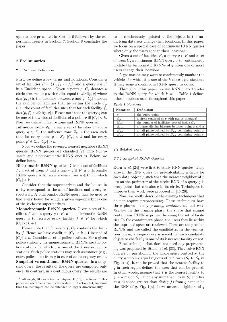
queries by partitioning the whole space centred at thequery q into six equal regions of 60∘ each (S1 to S6 in
Fig. 1(a)). It can be proved that the nearest facility to
q in each region defines the area that can be pruned.
In other words, assume that f is the nearest facility toq in a region Si. Then any user that lies in Si and lies
at a distance greater than dist(q, f) from q cannot be
the RNN of q. Fig. 1(a) shows nearest neighbors of q
4
in each region and the white area can be pruned. Only
the users that lie in the shaded area can be the RNNs.
The RkNN queries can be solved in a similar way, i.e.,
in each region, the k-th nearest facility of q defines the
pruned area.
Tao et al. [36] proposed TPL that uses the property
of perpendicular bisectors to prune the search space.
Consider the example of Fig. 1(b), where a bisectorbetween q and a is shown as Ba:q which divides the
space into two half-spaces. The half-space that contains
a is denoted as Ha:q and the half-space that contains q
is denoted as Hq:a. Any point that lies in the half-space
Ha:q is always closer to a than to q and cannot be theRNN for this reason. Similarly, any point p that lies in
k such half-spaces cannot be the RkNN. TPL algorithm
prunes the space by the bisectors drawn between q and
its neighbors in the unpruned area. Fig. 1(b) shows theexample where the bisectors between q and a, b and c
are drawn (Ba:q, Bb:q and Bc:q, respectively). If k = 2,
the white area can be pruned because every point in it
lies in at least two half-spaces.
S1
c
60o
S2S
3
S4 S
5S6
d
q 60o
a
b
e
f
g
(a) Six-regions pruning
b
a
Ba:q
Bb:q
Bc:q
qc
M
N
O P
(b) TPL and FINCH
Fig. 1 Related techniques
In the containment phase, TPL retrieves the users
that lie in the unpruned area by traversing an R-tree
that indexes the locations of the users. Let m be the
number of facility points for which the bisectors are con-sidered. An area that is the intersection of any combi-
nation of k half-spaces can be pruned. The total pruned
area corresponds to the union of pruned regions by all
such possible combinations of k bisectors (a total of
m!/k!(m−k)! combinations). Since the number of com-binations is too large, TPL uses an alternative approach
which has less pruning power but is cheaper. First, TPL
sorts the m facility points by their Hilbert values. Then,
only the combination of k consecutive facility points areconsidered to prune the space (total m combinations).
Achtert et al. [1] and Emrich et al. [13] propose
pruning techniques that can be applied on the rect-
angles. They use these pruning techniques to prune theintermediate entries of the R-tree that indexes the facil-
ities. It was demonstrated that the proposed techniques
reduce the number of accessed pages. Moreover, prun-
ing techniques proposed in [13] are more effective than
the pruning techniques of [1].
Wu et al. [41] propose an algorithm called FINCH.
Instead of using bisectors to prune the objects, they use
a convex polygon that approximates the unpruned area.
Any object that lies outside the polygon can be pruned.Fig. 1(b) shows an example where the shaded area is
the unpruned area. FINCH approximates the unpruned
area by a polygon MNOP . The algorithm can prune
the intermediate nodes of the R-tree and the objects
that lie outside this polygon. Clearly, the containmentchecking is cheaper than TPL (e.g., point containment
can be done in logarithmic time for convex polygons).
FINCH was shown to be superior to TPL [36].
It is worth mentioning that some of the existing
work focus on computing Voronoi cell (or order k Voronoi
cell) on the fly. More specifically, Stanoi et al. [34] com-pute Voronoi cell to answer RNN queries. On fly com-
putation of order k Voronoi cell was presented in [49,
18] to monitor kNN queries. Yiu et al. [46] study the
problem of common influence join and propose tech-niques for computing order k Voronoi cell on the fly.
Unfortunately, none of the above mentioned approaches
is applicable for RkNN queries. A straight forward ex-
tension is to compute several order k Voronoi cells and
join them to construct the influence zone. However, thisis computationally expensive because it requires con-
structing every order k Voronoi cell that contains q (see
Section 5.1). The pre-processing based approach is also
not suitable as discussed later in Section 5.1.
2.2.2 Continuous RNN Queries
Computation-efficient monitoring of continuous rangequeries [14,25,7], nearest neighbor queries [29,48,44,
21,37] and reverse nearest neighbor queries [2,42,23,
40] has received significant attention. Below, we briefly
describe the algorithms that monitor continuous RNNqueries.
Benetis et al. [2] presented the first continuous RNNmonitoring algorithm. However, they assume that ve-
locities of the objects are known. First work that does
not assume any knowledge of objects’ motion patterns
was presented by Xia et al. [42]. Their proposed so-lution is based on the six 60o regions based approach
described earlier in this section. Kang et al. [23] pro-
posed a continuous monitoring RNN algorithm based
on the bisector based (TPL) pruning approach. Both
of these algorithms continuously monitor RNN queriesby monitoring the unpruned area.
Wu et al. [40] propose the first technique to moni-
tor RkNNs. Their technique is based on the six-regions
based RNN monitoring presented in [42]. More specif-
5
ically, they issue k nearest neighbor (kNN) queries in
each region instead of the single nearest neighbor queries.
The users that are closer than the k-th NN in each re-
gion are the candidate objects and they are verified if q
is one of their k closest facilities. To monitor the results,for each candidate object, they continuously monitor
the circle around it that contains k nearest facilities.
Cheema et al. [10] propose Lazy Updates that is the
best known algorithm to continuously monitor RkNN
queries. Emrich et al. [12] independently proposed anapproach similar to Lazy Updates [10]. Lazy Updates
not only reduces the computation cost but also signif-
icantly reduces the communication cost. The existing
approaches call the expensive pruning phase wheneverthe query or a candidate object changes the location.
Lazy Updates saves the computation time by reduc-
ing the number of calls to the expensive pruning phase.
They assign each moving object a safe region and pro-
pose the pruning techniques to prune the space basedon the safe regions. The pruning phase is not needed to
be called as long as the related objects remain inside
their safe regions.
It is worth mentioning that all of the existing tech-
niques solve the general problem where every data pointincluding the query point is moving. In this paper, we
solve a special case of the problem where the facilities
do not move and the users are moving.
2.2.3 RNN queries under other settings
In this section, we provide an overview of the RNN
queries studied in other popular problem settings.
RNN queries in road networks. Yiu at al. [47] are
the first to study RNN queries in large graphs. They
present an interesting observation that is used to prune
the search space while traversing the graph in searchof RNN. Safar et al. [32] use Network Voronoi Diagram
(NVD) [30] to efficiently process the RNN queries in
spatial networks. In a following work [39], they extend
their technique to answer snapshot RkNN queries andreverse k furthest neighbor queries in spatial network.
Sun et al. [35] study the continuous monitoring of
RNN queries in spatial networks. The main idea is that
for each query a multi-way tree is created that helps in
defining the monitoring region. Only the updates in themonitoring region affect the results.
Li et al. [26] present a technique to continuously
monitor RkNN queries in spatial networks. They pro-
pose a novel data structure called dual layer multiway
tree (DLM tree) which is used to represent the mon-itoring region of RkNN queries. They present several
observations to reduce the size of the region that is to
be monitored for a RkNN query.
Cheema et al. [11] propose Lazy Updates that an-
swers continuous RkNN queries in Euclidean space as
well as in spatial networks. Each object and query is as-
signed a safe region and the expensive pruning phase is
not required as long as the query and relevant objectsremain in their respective safe regions. The proposed
technique reduces the computation cost as well as the
communication cost.
RNN queries on uncertain data. Probabilistic RNNqueries [8,27,3,4] has also received significant attention
from the research community. The basic idea behind
these techniques is as follows. Each uncertain object
and query is approximated by a rectangular [8,4] or a
circular [27] region. Pruning techniques are developedto prune the space based on these regions. Then, each
object that cannot be pruned is treated as a candidate
object and its probability of being the RNN is com-
puted.
3 Computing Influence Zone
3.1 Problem Characteristics
Given two facility points a and q, a perpendicular bi-
sector Ba:q between these two points divides the space
into two halves as shown in Fig 2(a). The half plane
that contains a is denoted as Ha:q and the half plane
that contains q is denoted as Hq:a. The perpendicularbisector has the property that any point p (depicted by
a star in Fig. 2(a)) that lies in Ha:q is closer to a than q
(i.e., dist(p, a) ≤ dist(p, q)) and any point y that lies in
Hq:a is closer to q than a (i.e., dist(y, q) ≤ dist(y, a)).Hence, q cannot be the closest facility of any point p
that lies in Ha:q, i.e., Cp contains at least one facility a.
We say that the point p is pruned by the bisector Ba:q
if p lies in Ha:q. Alternatively, we say that the point a
prunes the point p. In general, if a point p is pruned byat least k bisectors then Cp contains at least k facilities
(i.e., ∣Cp∣ ≥ k).
Existing work [36,41,10] use this observation to prune
the space that cannot contain any RkNN of q. Morespecifically, an area can be pruned if at least k bisec-
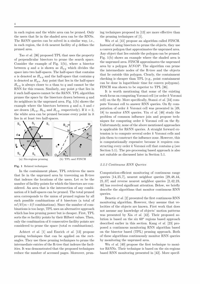
tors prune it. In Fig. 2, five facility points (q, a, b, c
and d) are shown. In Fig. 2(a) the bisectors between
q and two facility points a and b are drawn (see Ba:q
and Bb:q). If k is 2, then the white area can be prunedbecause it lies in two half-planes (Ha:q and Hb:q) and
∣Cp′ ∣ ≥ 2 for any point p′ in it. The area that is not
pruned is called unpruned area and is shown shaded.
Although it can be guaranteed that for every pointp′ in the pruned area ∣Cp′ ∣ ≥ k, it cannot be guaranteed
that for every point p in the unpruned area ∣Cp∣ < k if
we only consider a subset of the bisectors instead of all
6
q
a
b
cp
Ba:q
Bb:q
d
(a) Unpruned area is not influ-ence zone
q
a
b
c
Ba:q
Bb:q
Bc:q
d
Bd:q
(b) Unpruned area is influencezone
Fig. 2 Computing influence zone Zk (k = 2)
bisectors. In other words, the unpruned area is not the
influence zone. For example, in Fig. 2(a), the point plies in the unpruned area but ∣Cp∣ = 2 (i.e., Cp contains
a and c). Hence, the shaded area of Fig. 2(a) is not the
influence zone.
One straight forward approach to compute the in-
fluence zone is to consider the bisectors of q with every
facility point f . If the bisectors of q and all facilitiesare considered, then the unpruned area is the area that
is pruned by less than k bisectors. Fig. 2(b) shows the
unpruned area (the shaded polygon) after the bisectors
Bc:q and Bd:q are also considered. It can be verified thatthe shaded area is the influence zone (i.e., for every p
in the shaded area ∣Cp∣ < 2 and for every p′ outside it
∣Cp′ ∣ ≥ 2).
However, this straight forward approach is too ex-
pensive because it requires computing the bisectors be-
tween q and all facility points. We note that for some
facilities, we do not need to consider their bisectors. InFig. 2(b), it can be seen that the bisector Bd:q (shown in
broken line) does not affect the unpruned area (shown
shaded). In other words, if the bisectors of a, b and c
are considered then the bisector Bd:q does not prunemore area. Hence, even if Bd:q is ignored, the influence
zone can be computed.
Next, we present some lemmas that help us in iden-
tifying the facilities that can be ignored. Without loss of
generality, we assume that the data universe is bounded
by a square. Since we use bisectors to prune the space,the unpruned area is always a polygon and is inter-
changeably called unpruned polygon hereafter. Below
we present several lemmas that not only guide us to
the final lemma but also help us in few other proofs in
the paper.
Lemma 1 A facility f can be ignored if, for every
point p of the unpruned polygon, the facility f lies out-side Cp.
Proof As described earlier, a point p can be pruned
by the bisector Bf :q iff dist(p, f) < dist(p, q). In other
words, the point p can be pruned iff Cp contains f .
Hence, if f lies outside Cp, it cannot prune p. If f lies
outside Cp for every point p, it cannot prune any point
of the unpruned polygon and can be ignored for this
reason. ⊓⊔
Checking containment of f in Cp for every pointp is not feasible. In next few lemmas, we simplify the
procedure to check if a facility point can be ignored.
p
p'
q
(a) Lemma 2 and 3
qA
B
p
(b) Lemma 4
Fig. 3
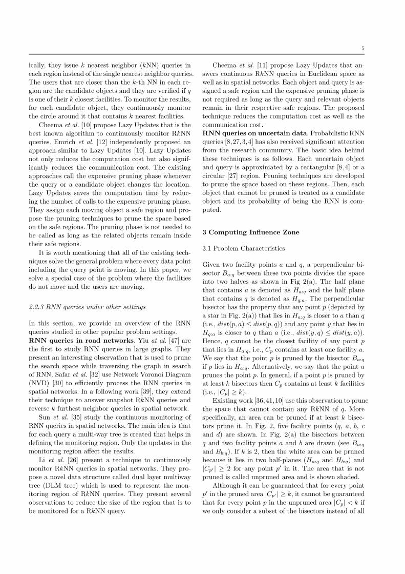
Lemma 2 Let pq be a line segment between two points
q and p. Let p′ be a point on pq. The circle Cp′ is con-tained by the circle Cp.
Fig. 3(a) shows an example where the circle Cp′ (the
shaded circle) is contained by Cp (the large circle). The
proof is straight forward and is omitted. Based on this
lemma, we present our next lemma.
Lemma 3 A facility f can be ignored if, for every
point p on the boundary of the unpruned polygon, f
lies outside Cp.
Proof We prove the lemma by showing that we do not
need to check containment of f in Cp′ for any point p′
that lies within the polygon. Let p′ be a point that
lies within the polygon. We draw a line that passes
through q and p′ and cuts the polygon at a point p
(see Fig. 3(a)). From Lemma 2, we know that Cp con-tains Cp′ . Hence, if f lies outside Cp, then it also lies
outside Cp′ . Hence, it suffices to check the containment
of f in Cp for every point p on the boundary of the
polygon. ⊓⊔
The next two lemmas show that we can check if a
facility f can be ignored or not by only checking thecontainment of f in Cv for every vertex v of the un-
pruned polygon.
Lemma 4 Given a line segment AB and a point p on
AB. The circle Cp is contained by CA ∪CB, i.e., everypoint in the circle Cp is either contained by CA or by
CB (see Fig. 3(b)).
7
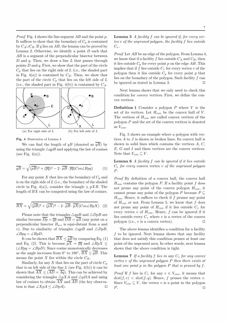
Proof Fig. 4 shows the line segmentAB and the point p.
It suffices to show that the boundary of Cp is contained
by CA∪CB . If q lies on AB, the lemma can be proved by
Lemma 2. Otherwise, we identify a point D such that
AB is a segment of the perpendicular bisector betweenD and q. Then, we draw a line L that passes through
pointsD and q. First, we show that the part of the circle
Cp that lies on the right side of L (i.e., the shaded part
in Fig. 4(a)) is contained by CB . Then, we show thatthe part of the circle Cp that lies on the left side of L
(i.e., the shaded part in Fig. 4(b)) is contained by CA.
q
X
A
B
EpD
L
(a) For right side of L
q
X
A
B
pD
L
(b) For left side of L
Fig. 4 Illustration of Lemma 4
We can find the length of qB (denoted as qB) by
using the triangle△qpB and applying the law of cosines(see Fig. 4(a)).
qB =
√
(pB)2 + (pq)2 − 2 ⋅ pB ⋅ pq(Cos∡Bpq) (1)
For any point X that lies on the boundary of Cp and
is on the right side of L (i.e., the boundary of the shaded
circle in Fig. 4(a)), consider the triangle △ pXB. Thelength of BX can be computed using the law of cosines.
BX =
√
(pB)2 + (pX)2 − 2 ⋅ pB ⋅ pX(Cos∡BpX) (2)
Please note that the triangles△qpB and △DpB are
similar because Dp = qp and DB = qB (any point on aperpendicular bisector Bu:v is equi-distant from u and
v). Due to similarity of triangles △qpB and △DpB,
∡Bpq = ∡BpD.
It can be shown thatBX ≤ qB by comparing Eq. (1)
and Eq. (2). This is because pX = pq and ∡BpX ≤
(∡Bpq = ∡BpD). Since cosine monotonically decreasesas the angle increases from 0∘ to 180∘, BX ≤ qB. This
means the point X lies within the circle CB.
Similarly, for any X that lies on the part of circle Cp
that is on left side of the line L (see Fig. 4(b)) it can be
shown that AX ≤ (AD = Aq). This can be achieved by
considering the triangles △pXA and △pDA and usinglaw of cosines to obtain AX and AD (the key observa-
tion is that ∡XpA ≤ ∡DpA). ⊓⊔
Lemma 5 A facility f can be ignored if, for every ver-
tex v of the unpruned polygon, the facility f lies outside
Cv.
Proof Let AB be an edge of the polygon. From Lemma 4,
we know that if a facility f lies outside CA and CB, thenit lies outside Cp for every point p on the edge AB. This
implies that if f lies outside Cv for every vertex v of the
polygon then it lies outside Cp for every point p that
lies on the boundary of the polygon. Such facility f canbe ignored as stated in Lemma 3. ⊓⊔
Next lemma shows that we only need to check this
condition for convex vertices. First, we define the con-
vex vertices.
Definition 1 Consider a polygon P where V is theset of its vertices. Let Hcon be the convex hull of V .
The vertices of Hcon are called convex vertices of the
polygon P and the set of the convex vertices is denoted
as Vcon.
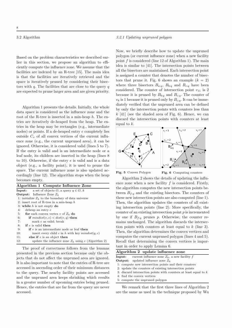
Fig. 5 shows an example where a polygon with ver-
tices A to J is shown in broken lines. Its convex hull is
shown in solid lines which contains the vertices A, C,
E, G and I and these vertices are the convex vertices.
Note that Vcon ⊆ V .
Lemma 6 A facility f can be ignored if it lies outside
Cv for every convex vertex v of the unpruned polygon
P .
Proof By definition of a convex hull, the convex hullHcon contains the polygon P . If a facility point f does
not prune any point of the convex polygon Hcon, it
cannot prune any point of the polygon P because P ⊆
Hcon. Hence, it suffices to check if f prunes any point
of Hcon or not. From Lemma 5, we know that f doesnot prune any point of Hcon if it lies outside Cv for
every vertex v of Hcon. Hence, f can be ignored if it
lies outside every Cv where v is a vertex of the convex
polygon (i.e., v is a convex vertex). ⊓⊔
The above lemma identifies a condition for a facility
f to be ignored. Next lemma shows that any facility
that does not satisfy this condition prunes at least one
point of the unpruned area. In other words, next lemma
shows that the above condition is tight.
Lemma 7 If a facility f lies in any Cv for any convex
vertex v of the unpruned polygon P then there exists at
least one point p in the polygon P that is pruned by f .
Proof If f lies in Cv for any v ∈ Vcon, it means thatdist(f, v) < dist(f, q). Hence, f prunes the vertex v.
Since Vcon ⊆ V , the vertex v is a point in the polygon
P . ⊓⊔
8
3.2 Algorithm
Based on the problem characteristics we described ear-
lier in this section, we propose an algorithm to effi-
ciently compute the influence zone. We assume that the
facilities are indexed by an R-tree [15]. The main idea
is that the facilities are iteratively retrieved and thespace is iteratively pruned by considering their bisec-
tors with q. The facilities that are close to the query q
are expected to prune larger area and are given priority.
Algorithm 1 presents the details. Initially, the wholedata space is considered as the influence zone and the
root of the R-tree is inserted in a min-heap ℎ. The en-
tries are iteratively de-heaped from the heap. The en-
tries in the heap may be rectangles (e.g., intermediate
nodes) or points. If a de-heaped entry e completely liesoutside Cv of all convex vertices of the current influ-
ence zone (e.g., the current unpruned area), it can be
ignored. Otherwise, it is considered valid (lines 5 to 7).
If the entry is valid and is an intermediate node or aleaf node, its children are inserted in the heap (lines 8
to 10). Otherwise, if the entry e is valid and is a data
object (e.g., a facility point), it is used to prune the
space. The current influence zone is also updated ac-
cordingly (line 12). The algorithm stops when the heapbecomes empty.
Algorithm 1 Compute Influence ZoneInput: a set of objects O, a query q ∈ O, kOutput: Influence Zone Zk
1: initialize Zk to the boundary of data universe2: insert root of R-tree in a min-heap ℎ3: while ℎ is not empty do
4: deheap an entry e5: for each convex vertex v of Zk do
6: if mindist(v, e) < dist(v, q) then
7: mark e as valid; break8: if e is valid then
9: if e is an intermediate node or leaf then
10: insert every child c in ℎ with key mindist(q, c)11: else if e is an object then
12: update the influence zone Zk using e (Algorithm 2)
The proof of correctness follows from the lemmas
presented in the previous section because only the ob-
jects that do not affect the unpruned area are ignored.It is also important to note that the entries of R-tree are
accessed in ascending order of their minimum distances
to the query. The nearby facility points are accessed
and the unpruned area keeps shrinking which resultsin a greater number of upcoming entries being pruned.
Hence, the entries that are far from the query are never
accessed.
3.2.1 Updating unpruned polygon
Now, we briefly describe how to update the unpruned
polygon (or current influence zone) when a new facility
point f is considered (line 12 of Algorithm 1). The mainidea is similar to [41]. The intersection points between
all the bisectors are maintained. Each intersection point
is assigned a counter that denotes the number of bisec-
tors that prune it. Fig. 6 shows an example (k = 2)
where three bisectors Ba:q, Bb:q and Bc:q have beenconsidered. The counter of intersection point v11 is 2
because it is pruned by Bb:q and Bc:q. The counter of
v8 is 1 because it is pruned only by Bc:q. It can be imme-
diately verified that the unpruned area can be definedby only the intersection points with counters less than
k [41] (see the shaded area of Fig. 6). Hence, we can
discard the intersection points with counters at least
equal to k.
qA
B
C
D
E
F
G
H
I
J
Fig. 5 Convex Polygon
q
v1 = 3
Ba:q
Bb:q
Bc:q
v2 = 1
v3 = 0v
6 = 2 v
5 = 1 v
4 = 0
v7 = 0
v8 = 1
v9 = 0
v10 = 0
v11 = 2
v12 = 2
Fig. 6 Computing counters
Algorithm 2 shows the details of updating the influ-ence zone when a new facility f is considered. Firstly,
the algorithm computes the new intersection points be-
tween Bf :q and the existing bisectors. The counters of
these new intersection points are also computed (line 1).Then, the algorithm updates the counters of all exist-
ing intersection points (line 2). More specifically, the
counter of an existing intersection point p is incremented
by one if Bf :q prunes p. Otherwise, the counter re-
mains unchanged. The algorithm discards the intersec-tion points with counters at least equal to k (line 3).
Then, the algorithm determines the convex vertices and
computes the current unpruned polygon (lines 4 and 5).
Recall that determining the convex vertices is impor-tant in order to apply Lemma 6.
Algorithm 2 update influence zoneInput: current influence zone Zk, a new facility fOutput: updated influence zone Zk
1: compute new intersection points and their counters2: update the counters of existing intersection points3: discard intersection points with counters at least equal to k4: find the convex vertices5: compute the unpruned polygon
We remark that the first three lines of Algorithm 2
are the same as used in the technique proposed by Wu
9
et. al [41]. They showed that the complexity of these
lines is O(m2) where m is the number of existing bi-
sectors contributing to the unpruned polygon. Later
in Section 5.4, we conduct a more rigorous complexity
analysis and show that the overall complexity of Algo-rithm 2 can be reduced to O(km) when k is smaller
than m.
3.2.2 Optimizations
In this section, we present few optimizations to improve
the efficiency of Algorithm 1. It can be shown that the
number of convex vertices is O(m) where m is the num-ber of bisectors considered so far [41] (i.e., m is the
number of facilities used to update the current influ-
ence zone at line 12 of Algorithm 1). Hence, checking
whether an entry of the R-tree is valid or not requires
O(m) distance computations (see lines 5 to 7 of Algo-rithm 1). Next, we present few observations and show
that we can determine the validity of some entries by a
single distance computation.
qA
B
CD
E
F
GH
I
rmin
rmax
p
e
(a) Lemma 8
q
rmax
p
e
(b) Lemma 9
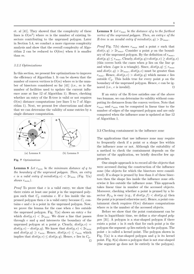
Fig. 7 Optimizations
Lemma 8 Let rmin be the minimum distance of q to
the boundary of the unpruned polygon. Then, an entry
e is a valid entry if mindist(q, e) < 2rmin (Fig. 7(a)shows rmin).
Proof To prove that e is a valid entry, we show that
there exists at least one point p in the unpruned poly-gon such that Cp contains e. If e lies inside the un-
pruned polygon then e is a valid entry because Ce con-
tains e and e is a point in the unpruned polygon. Now,
we prove the lemma for the case when e lies outside
the unpruned polygon. Fig. 7(a) shows an entry e forwhich dist(q, e) < 2rmin. We draw a line that passes
through e and q and intersects the boundary of the
unpruned polygon at a point p. Clearly, dist(p, e) =
dist(q, e)− dist(p, q). We know that dist(q, e) < 2rmin
and dist(p, q) ≥ rmin. Hence, dist(p, e) ≤ rmin which
implies that dist(p, e) ≤ dist(p, q). Hence, e lies in Cp.
⊓⊔
Lemma 9 Let rmax be the distance of q to the furthest
vertex of the unpruned polygon. Then, an entry e of the
R-tree is an invalid entry if mindist(e, q) > 2rmax.
Proof Fig. 7(b) shows rmax and a point e such that
dist(e, q) > 2rmax. Consider a point p on the bound-
ary of the unpruned polygon. By the definition of rmax,
dist(p, q) ≤ rmax. Clearly, dist(p, q)+dist(p, e) ≥ dist(q, e)(this covers both the cases when p lies on the line qe
and when △qpe is a triangle). Since, dist(p, q) ≤ rmax
and dist(e, q) > 2rmax, dist(p, e) must be greater than
rmax. Hence, dist(p, e) > dist(p, q) which means e liesoutside Cp. This holds true for every point p on the
boundary of the unpruned polygon. Hence, e can be ig-
nored (i.e., e is invalid). ⊓⊔
If an entry of the R-tree satisfies one of the above
two lemmas, we can determine its validity without com-
puting its distances from the convex vertices. Note that
rmax and rmin can be computed in linear time to thenumber of edges of the unpruned polygon and are only
computed when the influence zone is updated at line 12
of Algorithm 1.
3.3 Checking containment in the influence zone
The applications that use influence zone may require
to frequently check if a point or a shape lies within
the influence zone or not. Although the suitability of
a method to check the containment depends on thenature of the application, we briefly describe few ap-
proaches.
One simple approach is to record all the objects that
were accessed during the construction of the influencezone (the objects for which the bisectors were consid-
ered). If a shape is pruned by less than k of these bisec-
tors then the shape lies inside the influence zone oth-
erwise it lies outside the influence zone. This approachtakes linear time in number of the accessed objects.
Moreover, checking whether a point is pruned by a bi-
sector Bf :q is easy (e.g., if dist(p, f) < dist(p, q) then
the point p is pruned otherwise not). Hence, a point con-
tainment check requires O(m) distance computationswhere m is the number of the accessed objects.
Before we show that the point containment can be
done in logarithmic time, we define a star-shaped poly-gon [31]. A polygon is a star-shaped polygon if there
exists a point z in it such that for each point p in the
polygon the segment zp lies entirely in the polygon. The
point z is called a kernel point. The polygon shown inFig. 7(a) is a star-shaped polygon and q is its kernel
point. Fig. 8(a) shows a polygon that is not star-shaped
(the segment qp does not lie entirely in the polygon).
10
Let n be the number of vertices of a star-shaped poly-
gon. After a linear time pre-processing, every point con-
tainment check can be done in O(log n) if a kernel point
of the polygon is known [31]. Please see [31] for more
details.
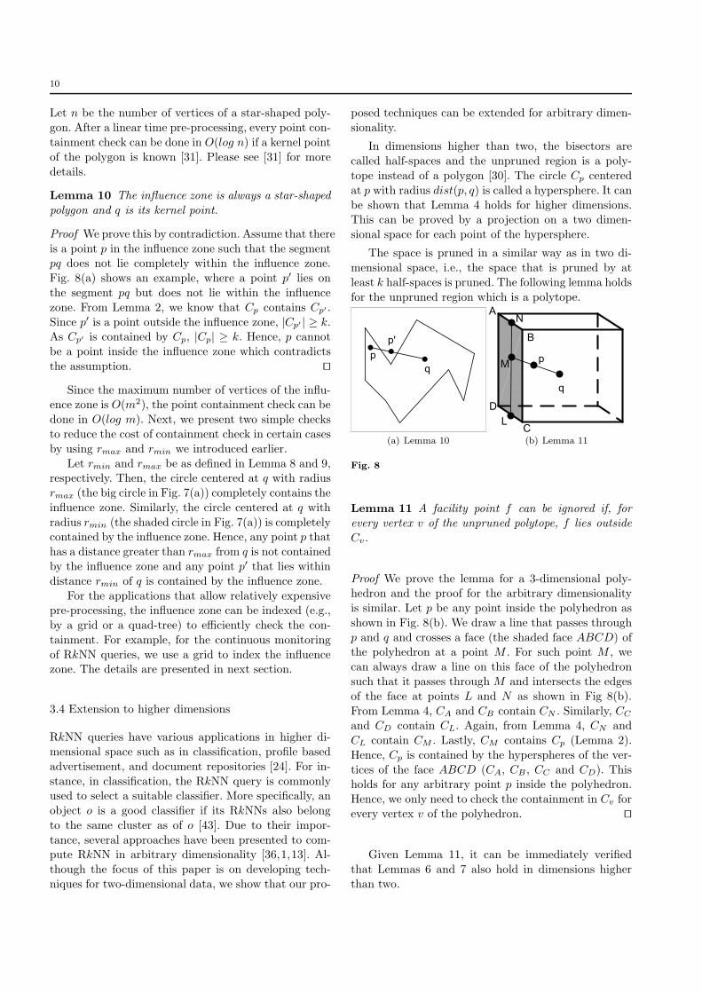
Lemma 10 The influence zone is always a star-shaped
polygon and q is its kernel point.
Proof We prove this by contradiction. Assume that there
is a point p in the influence zone such that the segmentpq does not lie completely within the influence zone.
Fig. 8(a) shows an example, where a point p′ lies on
the segment pq but does not lie within the influence
zone. From Lemma 2, we know that Cp contains Cp′ .
Since p′ is a point outside the influence zone, ∣Cp′ ∣ ≥ k.As Cp′ is contained by Cp, ∣Cp∣ ≥ k. Hence, p cannot
be a point inside the influence zone which contradicts
the assumption. ⊓⊔
Since the maximum number of vertices of the influ-ence zone is O(m2), the point containment check can be
done in O(log m). Next, we present two simple checks
to reduce the cost of containment check in certain cases
by using rmax and rmin we introduced earlier.
Let rmin and rmax be as defined in Lemma 8 and 9,respectively. Then, the circle centered at q with radius
rmax (the big circle in Fig. 7(a)) completely contains the
influence zone. Similarly, the circle centered at q with
radius rmin (the shaded circle in Fig. 7(a)) is completelycontained by the influence zone. Hence, any point p that
has a distance greater than rmax from q is not contained
by the influence zone and any point p′ that lies within
distance rmin of q is contained by the influence zone.
For the applications that allow relatively expensivepre-processing, the influence zone can be indexed (e.g.,
by a grid or a quad-tree) to efficiently check the con-
tainment. For example, for the continuous monitoring
of RkNN queries, we use a grid to index the influencezone. The details are presented in next section.
3.4 Extension to higher dimensions
RkNN queries have various applications in higher di-
mensional space such as in classification, profile based
advertisement, and document repositories [24]. For in-
stance, in classification, the RkNN query is commonlyused to select a suitable classifier. More specifically, an
object o is a good classifier if its RkNNs also belong
to the same cluster as of o [43]. Due to their impor-
tance, several approaches have been presented to com-pute RkNN in arbitrary dimensionality [36,1,13]. Al-
though the focus of this paper is on developing tech-
niques for two-dimensional data, we show that our pro-
posed techniques can be extended for arbitrary dimen-
sionality.
In dimensions higher than two, the bisectors are
called half-spaces and the unpruned region is a poly-
tope instead of a polygon [30]. The circle Cp centered
at p with radius dist(p, q) is called a hypersphere. It can
be shown that Lemma 4 holds for higher dimensions.This can be proved by a projection on a two dimen-
sional space for each point of the hypersphere.
The space is pruned in a similar way as in two di-
mensional space, i.e., the space that is pruned by at
least k half-spaces is pruned. The following lemma holds
for the unpruned region which is a polytope.
p
p'
q
(a) Lemma 10
q
A
B
C
D
pM
N
L
(b) Lemma 11
Fig. 8
Lemma 11 A facility point f can be ignored if, forevery vertex v of the unpruned polytope, f lies outside
Cv.
Proof We prove the lemma for a 3-dimensional poly-hedron and the proof for the arbitrary dimensionality
is similar. Let p be any point inside the polyhedron as
shown in Fig. 8(b). We draw a line that passes through
p and q and crosses a face (the shaded face ABCD) ofthe polyhedron at a point M . For such point M , we
can always draw a line on this face of the polyhedron
such that it passes through M and intersects the edges
of the face at points L and N as shown in Fig 8(b).
From Lemma 4, CA and CB contain CN . Similarly, CC
and CD contain CL. Again, from Lemma 4, CN and
CL contain CM . Lastly, CM contains Cp (Lemma 2).
Hence, Cp is contained by the hyperspheres of the ver-
tices of the face ABCD (CA, CB , CC and CD). Thisholds for any arbitrary point p inside the polyhedron.
Hence, we only need to check the containment in Cv for
every vertex v of the polyhedron. ⊓⊔
Given Lemma 11, it can be immediately verified
that Lemmas 6 and 7 also hold in dimensions higher
than two.
11
4 Applications in RkNN Processing
4.1 Snapshot Bichromatic RkNN Queries
Our algorithm consists of two phases namely pruning
phase and containment phase.
Pruning Phase. In this phase, the influence zone Zk
is computed using the given set of facilities.
Containment Phase. By the definition of influence
zone Zk, a user u can be the bichromatic RkNN if and
only if it lies within the influence zone Zk. We assume
that the set of users are indexed by an R-tree. TheR-tree is traversed and the entries that lie outside the
influence zone are pruned. The objects that lie in the
influence zone are RkNNs.
4.2 Snapshot Monochromatic RkNN Queries
By definition of a monochromatic RkNN query (see Sec-
tion 2.1), a facility f is the RkNN iff ∣Cf ∣ < k+1. Hence,
a facility that lies in Zk+1 is the monochromatic RkNN
of q where Zk+1 is the influence zone computed by set-ting k to k + 1. Below, we highlight our technique.
Pruning Phase. In this phase, we compute the influ-
ence zone Zk+1 using the given set of facilities F . We
also record the facility points that are accessed duringthe construction of the influence zone and call them the
candidate objects.
Containment Phase. Please note that every facility
point that is contained in the influence zone Zk+1 willbe accessed during the pruning phase. This is because
every facility that lies in the influence zone cannot be
ignored during the construction of the influence zone
(inferred from Lemma 1). Hence, the set of candidateobject contains all possible RkNNs. For each of the can-
didate object, we report it as RkNN if it lies within the
influence zone Zk+1.
4.3 Continuous monitoring of RkNNs
In this section, we present our technique to continuously
monitor bichromatic RkNN queries (see the problem
definition in Section 2.1). The basic idea is to index
the influence zone by a grid. Then, the RkNNs can bemonitored by tracking the users that enter or leave the
influence zone.
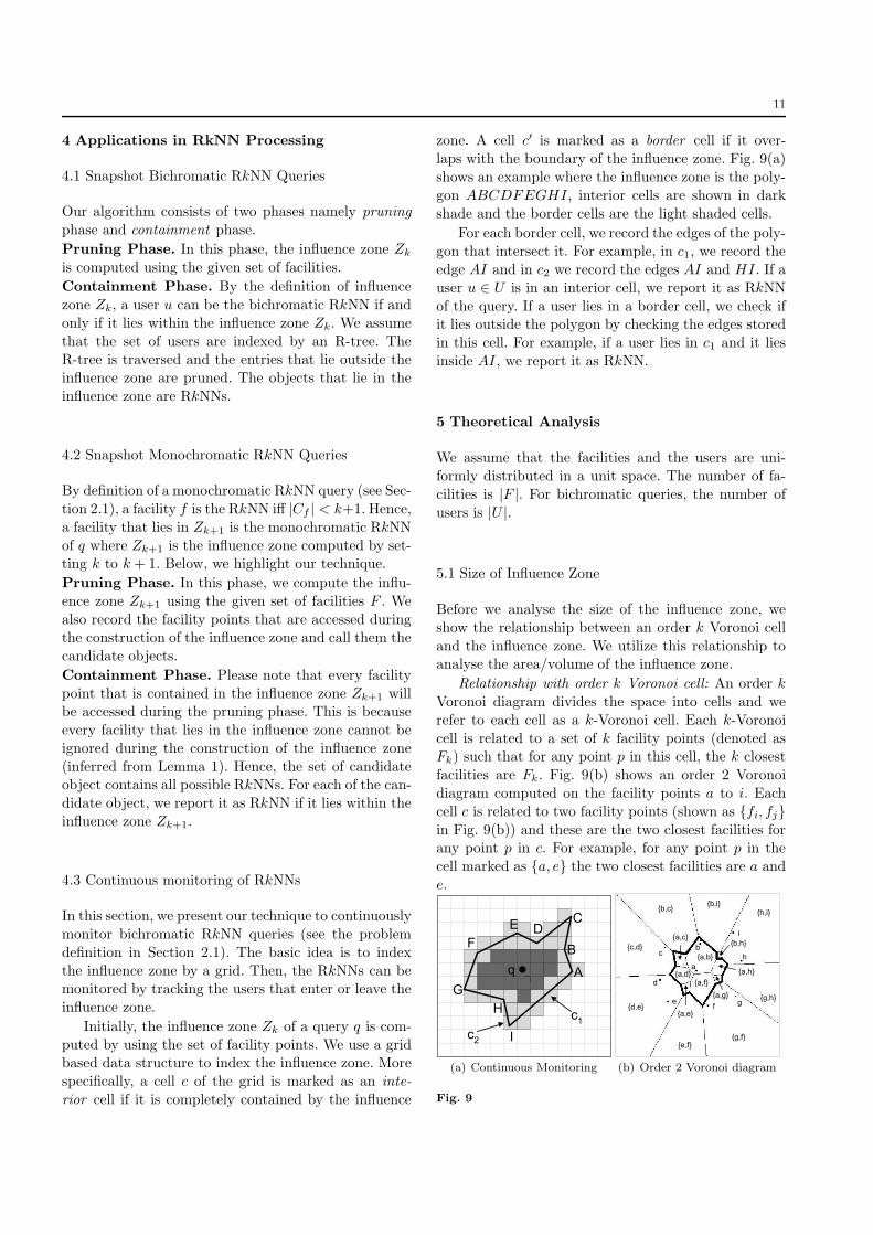
Initially, the influence zone Zk of a query q is com-
puted by using the set of facility points. We use a gridbased data structure to index the influence zone. More
specifically, a cell c of the grid is marked as an inte-
rior cell if it is completely contained by the influence
zone. A cell c′ is marked as a border cell if it over-
laps with the boundary of the influence zone. Fig. 9(a)
shows an example where the influence zone is the poly-
gon ABCDFEGHI, interior cells are shown in dark
shade and the border cells are the light shaded cells.
For each border cell, we record the edges of the poly-gon that intersect it. For example, in c1, we record the
edge AI and in c2 we record the edges AI and HI. If a
user u ∈ U is in an interior cell, we report it as RkNN
of the query. If a user lies in a border cell, we check ifit lies outside the polygon by checking the edges stored
in this cell. For example, if a user lies in c1 and it lies
inside AI, we report it as RkNN.
5 Theoretical Analysis
We assume that the facilities and the users are uni-
formly distributed in a unit space. The number of fa-
cilities is ∣F ∣. For bichromatic queries, the number of
users is ∣U ∣.
5.1 Size of Influence Zone
Before we analyse the size of the influence zone, we
show the relationship between an order k Voronoi cell
and the influence zone. We utilize this relationship toanalyse the area/volume of the influence zone.
Relationship with order k Voronoi cell: An order k
Voronoi diagram divides the space into cells and we
refer to each cell as a k-Voronoi cell. Each k-Voronoi
cell is related to a set of k facility points (denoted asFk) such that for any point p in this cell, the k closest
facilities are Fk. Fig. 9(b) shows an order 2 Voronoi
diagram computed on the facility points a to i. Each
cell c is related to two facility points (shown as {fi, fj}
in Fig. 9(b)) and these are the two closest facilities forany point p in c. For example, for any point p in the
cell marked as {a, e} the two closest facilities are a and
e.
q A
B
CDE
F
G
H
I
c1
c2
(a) Continuous Monitoring
a
cb
d
ef
i
g
h{a,b}
{a,h}
{a,g}
{a,f}
{a,e}
{a,d}
{a,c}{b,h}
{h,i}
{g,h}
{g,f}{e,f}
{d,e}
{c,d}
{b,i}{b,c}
(b) Order 2 Voronoi diagram
Fig. 9
12
Clearly, when k = 1 the k-Voronoi cell related to q
is exactly the same as the influence zone. For k > 1, the
influence zone corresponds to the union of all k-Voronoi
cells that are related to q (i.e., have q in their Fk). For
example, in Fig. 9(b), the influence zone of the facilitya is shown in bold boundary and it corresponds to the
union of the cells related to a.
Now, we analyse the area of the influence zone.
Consider the influence zones of all the facilities in
the data set. Every point in the unit space lies in a cell
that is related to k facilities. This implies that every
point lies in exactly k influence zones (e.g., in Fig. 9(b),every point in the cell marked as {a, f} lies in the influ-
ence zone of a as well as the influence zone of f). Hence,
the sum of the areas of all the influence zones is k. Since
the total number of facility points is ∣F ∣, the expected
area of a randomly chosen facility point is k/∣F ∣.
Note that the above discussion does not depend on
the dimensionality. Hence, the volume of the influence
zone is k/∣F ∣ regardless of the dimensionality.
Remark: The above discussion shows that the influ-ence zone can be computed by using a pre-computed or-
der k Voronoi diagram. However, as mentioned in [49],
a technique that uses a pre-computed order k Voronoi
diagram may not be practical for the following reasons :
i) the value of k may not be known in advance; ii) evenif k is known in advance, order k Voronoi diagrams are
very expensive to compute and incur high space require-
ment; iii) spatial indexes are useful for all query types
and pre-computed Voronoi diagrams may not be usedfor all queries. In contrast, R-tree based indexes used
by our algorithm are used for many important queries.
5.2 Result size of RkNN queries
First, we analyse the result size for bichromatic RkNNs
queries. We assume that the users are uniformly dis-
tributed in the space. Recall that every user that lies
in the influence zone is a bichromatic RkNN object.Hence, the expected result size (i.e., number of bichro-
matic RkNNs) can be obtained by multiplying ∣U ∣ with
the expected area (volume for higher dimensionality)
of the influence zone. Hence, the expected number of
bichromatic RkNNs is ∣U ∣.k/∣F ∣ (regardless of the di-mensionality).
Now, we analyse the result size for monochromatic
RkNN queries. The area/volume of the influence zone
Zk+1 for a monochromatic RkNN query is (k+ 1)/∣F ∣.The number of facilities in this zone is (k+1) which in-
cludes the query. Hence the expected number of monochro-
matic RkNNs is k (regardless of the dimensionality).
5.3 IO cost of our algorithms
In this section, we present IO cost analysis for our algo-
rithms which is applicable to arbitrary dimensionality.
Before we analyse the IO costs of our proposed algo-
rithms, we analyse the cost of a circular range query ind-dimensional space. Then, we analyse the costs of our
algorithms by using the IO cost of the circular range
queries.
5.3.1 IO cost of a circular range query
A circular range query [6] finds the objects that lie
within distance r of the query location. We assume that
the objects are indexed by an R-tree and analyse thenumber of nodes that lie within the range of the query.
The approach to analyse the IO cost of the circular
range query is similar to the IO cost analysis of window
queries presented in [38]. Assume a hypersphere in a d-dimensional space that has a radius R. Let VR denote
the volume of this hypersphere. Let Nl be the number
of rectangles at level l of the R-tree. We assume that the
centers of the rectangles at each level follow a uniform
distribution. The expected number of rectangles at alevel l that have their centers in the hypersphere is VR×
Nl.
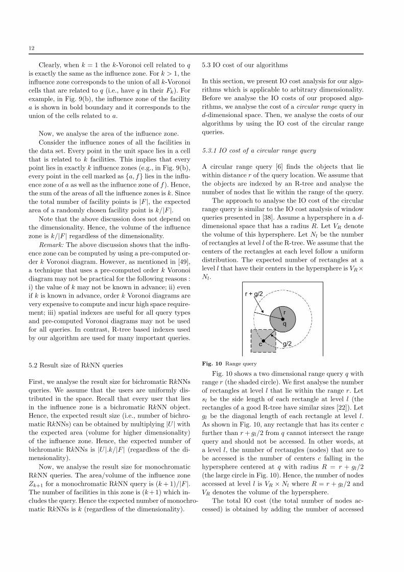
Fig. 10 Range query
Fig. 10 shows a two dimensional range query q withrange r (the shaded circle). We first analyse the number
of rectangles at level l that lie within the range r. Let
sl be the side length of each rectangle at level l (the
rectangles of a good R-tree have similar sizes [22]). Let
gl be the diagonal length of each rectangle at level l.As shown in Fig. 10, any rectangle that has its center c
further than r+ gl/2 from q cannot intersect the range
query and should not be accessed. In other words, at
a level l, the number of rectangles (nodes) that are tobe accessed is the number of centers c falling in the
hypersphere centered at q with radius R = r + gl/2
(the large circle in Fig. 10). Hence, the number of nodes
accessed at level l is VR × Nl where R = r + gl/2 and
VR denotes the volume of the hypersphere.
The total IO cost (the total number of nodes ac-
cessed) is obtained by adding the number of accessed
13
nodes for each level l. The total number of levels ex-
cluding the root is ⌊logfS⌋ where f is the fanout of
R-tree and S is the total number of objects indexed
by the R-tree. The root is accessed anyway, so one is
added to this cost. Hence, the total IO cost is obtainedby Eq. (3).
Range query cost = 1 +
⌊logfS⌋∑
l=1
VR ×Nl (3)
Now, we need to compute VR, and Nl for each level
l. To compute VR, we need to compute gl. The numberof rectangles Nl at level l of the R-tree is S/f
l (e.g., leaf
nodes are at level 1 and the number of leaf level rect-
angles is S/f). Since we assume uniform distribution of
points, each rectangle at level l contains f l points. Inother words, the area/volume of each node (rectangle)
is f l/S. Assuming that the side length of a rectangle
on each dimension is the same, the side length sl is
(f l/S)1/d. Given sl of a rectangle, the diagonal length
gl can be computed by using Eq. (4).
gl =
√
√
√
⎷
d∑
i=1
s2l =
√
√
√
⎷
d∑
i=1
(f l
S)
2d =
√
d× (f l
S)
2d (4)
Finally, we need to compute VR. Let R be the radius
of a hypersphere. The volume VR of the hypersphere isVR = Cd × Rd where d denotes the dimensionality of
the hypersphere2. Cd for even dimensionality is �d/2
(d/2)!
where x! denotes the factorial of a number x. Cd for
odd dimensionality is 2(d+1)/2�(d−1)/2
d!! where x!! denotes
the double factorial of x. The double factorial of x is
the multiplication of all odd numbers from 1 to x.
By using gl shown in Eq. (4), we can compute R(and VR). Plugging the values of VR and Nl in Eq. (3)
gives us the IO cost of the range query. Based on the
IO cost of the range query, first we analyse the cost of
computing the influence zone and then we analyse thecosts of our RkNN algorithms.
5.3.2 IO cost of computing the influence zone
We approximate the influence zone to a hyperspherical
region that has the same area/volume as that of the in-
fluence zone (we noted that as k gets larger the shape of
the influence zone has more resemblance with a hyper-
sphere). Since the area/volume of the influence zone Zk
is k/∣F ∣, the radius rk of the hypersphere can be com-
puted. More specifically, Vrk = k/∣F ∣ = Cd × rdk which
implies that rk = ( k∣F ∣×Cd
)1/d. As implied by Lemma 5,
2 http://www.en.wikipedia.org/wiki/N-sphere
an object can be ignored if it lies at a distance greater
than dist(q, v) from every vertex v of the unpruned re-
gion. Since we assume that each vertex is at the same
distance rk from the query (i.e., influence zone is a hy-
persphere), an object can be ignored if it lies at a dis-tance greater than 2rk from q. Hence, the objects within
the range 2rk of the query are accessed during the com-
putation of the influence zone. The IO cost is then the
cost of a range query with range 2rk = 2( k∣F ∣×Cd
)1/d.
5.3.3 IO cost of a monochromatic RkNN query
The IO cost for a monochromatic RkNN query is the
same as the IO cost of computing the influence zone
Zk+1. This is because the R-tree is traversed only dur-
ing the construction of the influence zone (i.e., the con-
tainment phase does not access R-tree). Hence, IO costof a monochromatic query is the IO cost of a range
query with range set as 2rk+1 = 2( k+1∣F ∣×Cd
)1/d.
5.3.4 IO cost of a bichromatic RkNN query
The cost of the pruning phase is the same as the cost of
computing the influence zone Zk which we have anal-
ysed earlier. The cost of the containment phase is thecost of accessing the users that lie within the influence
zone which can be computed in a similar way. More
specifically, only the users that lie within distance rk(the radius of the influence zone) of q are accessed.Hence, the cost of the containment phase is the IO cost
of the range query with range set to rk = 2( k∣F ∣×Cd
)1/d.
5.4 Complexity Analysis
The complexity of Algorithm 2 for arbitrarily dimen-
sionality d is exponential in d because the number of
intersection points of m half-spaces in d dimensionalspace is O(md). Nevertheless, our experimental results
demonstrate that the performance of our algorithms is
reasonable as compared to other approaches (for di-
mensionality up to 4). In this section, we show that the
complexity of Algorithm 2 in two dimensional spacecan be reduced from O(m2) to O(km) where m is the
number of facilities (or bisectors) considered so far. In
the rest of the paper, our discussion is based on two
dimensional space unless specifically mentioned other-wise. Below, we define a few terms and notations and
present a lemma that helps us in analysing the com-
plexity.
14
5.4.1 Preliminaries
Valid intersection point. An intersection point that
has a counter less than k is called a valid intersectionpoint.
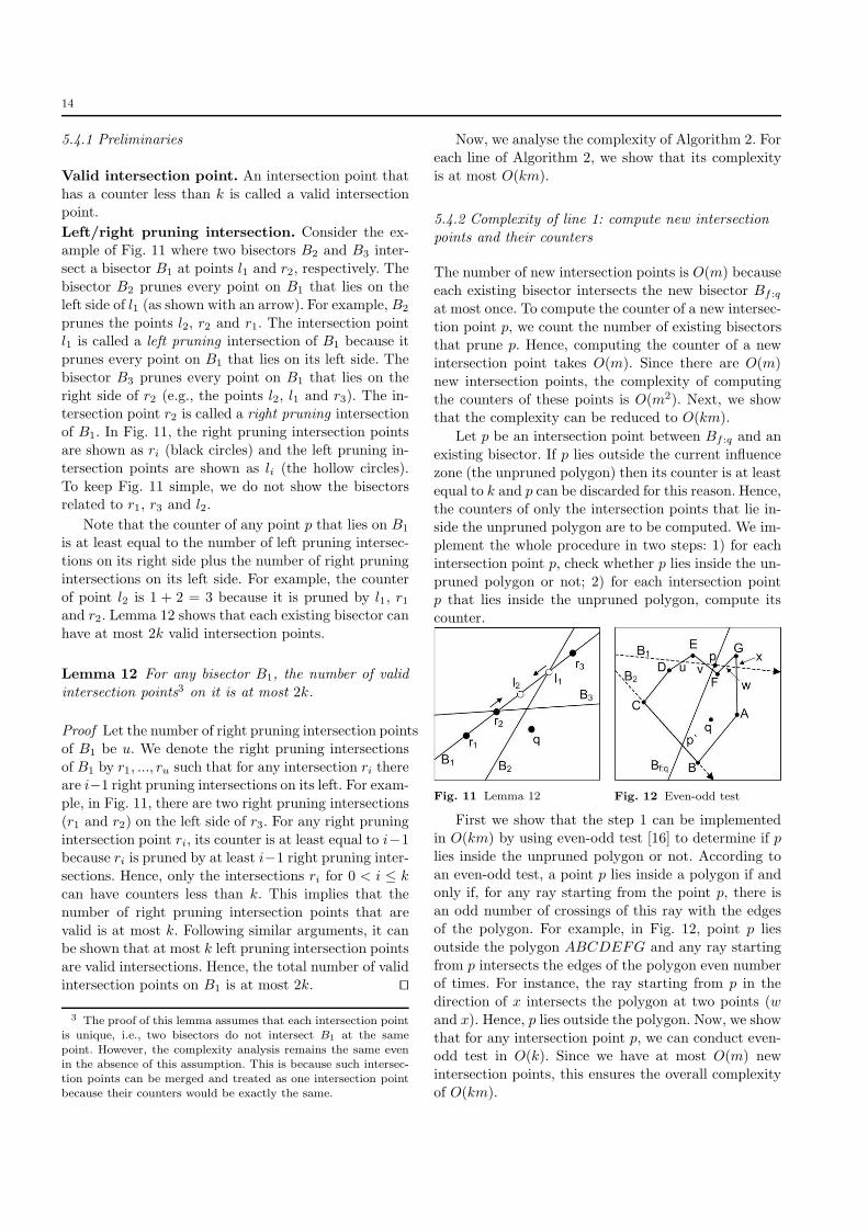
Left/right pruning intersection. Consider the ex-ample of Fig. 11 where two bisectors B2 and B3 inter-
sect a bisector B1 at points l1 and r2, respectively. The
bisector B2 prunes every point on B1 that lies on the
left side of l1 (as shown with an arrow). For example, B2
prunes the points l2, r2 and r1. The intersection pointl1 is called a left pruning intersection of B1 because it
prunes every point on B1 that lies on its left side. The
bisector B3 prunes every point on B1 that lies on the
right side of r2 (e.g., the points l2, l1 and r3). The in-tersection point r2 is called a right pruning intersection
of B1. In Fig. 11, the right pruning intersection points
are shown as ri (black circles) and the left pruning in-
tersection points are shown as li (the hollow circles).
To keep Fig. 11 simple, we do not show the bisectorsrelated to r1, r3 and l2.
Note that the counter of any point p that lies on B1
is at least equal to the number of left pruning intersec-
tions on its right side plus the number of right pruning
intersections on its left side. For example, the counter
of point l2 is 1 + 2 = 3 because it is pruned by l1, r1and r2. Lemma 12 shows that each existing bisector can
have at most 2k valid intersection points.
Lemma 12 For any bisector B1, the number of valid
intersection points3 on it is at most 2k.
Proof Let the number of right pruning intersection points
of B1 be u. We denote the right pruning intersections
of B1 by r1, ..., ru such that for any intersection ri thereare i−1 right pruning intersections on its left. For exam-
ple, in Fig. 11, there are two right pruning intersections
(r1 and r2) on the left side of r3. For any right pruning
intersection point ri, its counter is at least equal to i−1because ri is pruned by at least i−1 right pruning inter-
sections. Hence, only the intersections ri for 0 < i ≤ k
can have counters less than k. This implies that the
number of right pruning intersection points that are
valid is at most k. Following similar arguments, it canbe shown that at most k left pruning intersection points
are valid intersections. Hence, the total number of valid
intersection points on B1 is at most 2k. ⊓⊔
3 The proof of this lemma assumes that each intersection pointis unique, i.e., two bisectors do not intersect B1 at the samepoint. However, the complexity analysis remains the same evenin the absence of this assumption. This is because such intersec-tion points can be merged and treated as one intersection pointbecause their counters would be exactly the same.
Now, we analyse the complexity of Algorithm 2. For
each line of Algorithm 2, we show that its complexity
is at most O(km).
5.4.2 Complexity of line 1: compute new intersection
points and their counters
The number of new intersection points is O(m) because
each existing bisector intersects the new bisector Bf :q
at most once. To compute the counter of a new intersec-
tion point p, we count the number of existing bisectorsthat prune p. Hence, computing the counter of a new
intersection point takes O(m). Since there are O(m)
new intersection points, the complexity of computing
the counters of these points is O(m2). Next, we showthat the complexity can be reduced to O(km).
Let p be an intersection point between Bf :q and an
existing bisector. If p lies outside the current influence
zone (the unpruned polygon) then its counter is at least
equal to k and p can be discarded for this reason. Hence,
the counters of only the intersection points that lie in-side the unpruned polygon are to be computed. We im-
plement the whole procedure in two steps: 1) for each
intersection point p, check whether p lies inside the un-
pruned polygon or not; 2) for each intersection pointp that lies inside the unpruned polygon, compute its
counter.
Fig. 11 Lemma 12 Fig. 12 Even-odd test
First we show that the step 1 can be implemented
in O(km) by using even-odd test [16] to determine if p
lies inside the unpruned polygon or not. According to
an even-odd test, a point p lies inside a polygon if andonly if, for any ray starting from the point p, there is
an odd number of crossings of this ray with the edges
of the polygon. For example, in Fig. 12, point p lies
outside the polygon ABCDEFG and any ray starting
from p intersects the edges of the polygon even numberof times. For instance, the ray starting from p in the
direction of x intersects the polygon at two points (w
and x). Hence, p lies outside the polygon. Now, we show
that for any intersection point p, we can conduct even-odd test in O(k). Since we have at most O(m) new
intersection points, this ensures the overall complexity
of O(km).
15
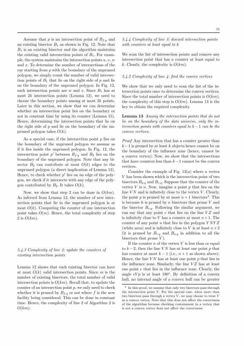
Assume that p is an intersection point of Bf :q and
an existing bisector B1 as shown in Fig. 12. Note that
B1 is an existing bisector and the algorithm maintains
the existing valid intersection points of B1. For exam-
ple, the system maintains the intersection points u, v, wand x. To determine the number of intersections of the
ray starting from p with the boundary of the unpruned
polygon, we simply count the number of valid intersec-
tion points of B1 that lie on the right side of p and lieon the boundary of the unpruned polygon. In Fig. 12,
such intersection points are w and x. Since B1 has at
most 2k intersection points (Lemma 12), we need to
choose the boundary points among at most 2k points.
Later in this section, we show that we can determinewhether an intersection point lies on the boundary or
not in constant time by using its counter (Lemma 15).
Hence, determining the intersection points that lie on
the right side of p and lie on the boundary of the un-pruned polygon takes O(k).
As a special case, if the intersection point p lies on
the boundary of the unpruned polygon we assume as
if it lies inside the unpruned polygon. In Fig. 12, the
intersection point p′ between Bf :q and B2 lies on theboundary of the unpruned polygon. Note that any bi-
sector B2 can contribute at most O(k) edges to the
unpruned polygon (a direct implication of Lemma 12).
Hence, to check whether p′ lies on an edge of the poly-
gon, we check if it intersects with any edge of the poly-gon contributed by B2. It takes O(k).
Now, we show that step 2 can be done in O(km).
As inferred from Lemma 12, the number of new inter-
section points that lie in the unpruned polygon is at
most O(k). Computing the counter of one intersectionpoint takes O(m). Hence, the total complexity of step
2 is O(km).
5.4.3 Complexity of line 2: update the counters of
existing intersection points
Lemma 12 shows that each existing bisector can have
at most O(k) valid intersection points. Since m is thenumber of existing bisectors, the total number of valid
intersection points is O(km). Recall that, to update the
counter of an intersection point p, we only need to check
whether it is pruned by Bf :q or not where f is the newfacility being considered. This can be done in constant
time. Hence, the complexity of line 2 of Algorithm 2 is
O(km).
5.4.4 Complexity of line 3: discard intersection points
with counters at least equal to k
We scan the list of intersection points and remove anyintersection point that has a counter at least equal to
k. Clearly, the complexity is O(km).
5.4.5 Complexity of line 4: find the convex vertices
We show that we only need to scan the list of the in-
tersection points once to determine the convex vertices.
Since the total number of intersection points is O(km),
the complexity of this step is O(km). Lemma 13 is thekey to obtain the required complexity.
Lemma 13 Among the intersection points that do not
lie on the boundary of the data universe, only the in-tersection points with counters equal to k− 1 can be the
convex vertices.
Proof Any intersection that has a counter greater than
k−1 is pruned by at least k objects hence cannot be on
the boundary of the influence zone (hence, cannot be
a convex vertex). Now, we show that the intersectionsthat have counters less than k−1 cannot be the convex
vertices.
Consider the example of Fig. 13(a) where a vertex
V has been shown which is the intersection point of two
bisectors Ba:q and Bc:q. Suppose that the counter of the
vertex V is n. Now, imagine a point p that lies on theline V N and is infinitely close to the vertex V . Clearly,
the point p is pruned by at most n+ 1 bisectors4. This
is because it is pruned by n bisectors that prune V and
the bisector Bc:q. Following the similar argument, we
can say that any point e that lies on the line V Z andis infinitely close to V has a counter at most n+1. The
counter of any point u that lies in the polygon V NY Z
(white area) and is infinitely close to V is at least n+2
(it is pruned by Bc:q and Ba:q in addition to all thebisectors that prune V ).
If the counter n of the vertex V is less than or equalto k− 2, then the line V N has at least one point p that
has counter at most k − 1 (i.e., n+ 1 as shown above).
Hence, the line V N has at least one point p that lies in
the influence zone. Similarly, the line V Z has at leastone point e that lies in the influence zone. Clearly, the
angle eV p is at least 180∘. By definition of a convex
hull, no internal angle of a convex hull can be greater
4 In this proof, we assume that only two bisectors pass throughthe intersection point V . For the special case, when more thantwo bisectors pass through a vertex V , we may choose to treat Vas a convex vertex. Note that this does not affect the correctnessof the algorithm because checking containment in a vertex thatis not a convex vertex does not affect the correctness.

16
than 1800. Hence, the vertex V is not a convex vertex
if its counter is less than or equal to k − 2. ⊓⊔
(a) Lemma 13 (b) Counters
Fig. 13 Finding convex vertices
In Fig. 13(b), we revisit the example of Fig. 6. The
vertices v7 and v9 do not lie on the boundary of the data
universe and have counters less than k − 1 (where k =
2). Hence, they are not the convex vertices. Among thepoints that lie on the boundary of the data universe and
have counters less than k, only the two extreme points
for each boundary line can be the convex vertices. For
example, in Fig. 6, the lower horizontal boundary linecontains 4 vertices (v3, v4, v5 and v6). The vertex v6has counter not less than k and can be ignored. Among
the remaining vertices, we consider the extreme vertices
(v3 and v5) as the convex vertices. Following the above
strategy, the convex vertices in Fig. 6 are v3, v2, v8 andv5.
The above discussion shows that the convex vertices
can be found by scanning the list of intersection points
once. Hence, the cost of finding the convex vertices isO(km).
5.4.6 Complexity of line 5: compute the unpruned
polygon
For any point p, we use �p to denote the angle formed
by the horizontal line passing through q and the line
segment pq (see Fig. 13(b)). Recall that line 1 addsO(k) new intersection points. These intersection points
are always inserted in sorted order of �p and this takes
O(k ⋅ log m) because O(k) points are inserted and each
insertion takes O(log m) (the maximum number of ex-
isting intersection points is O(m2)). Next, we show thatthe unpruned polygon can be computed in O(km) if all
the intersection points are sorted according to �p.
Lemma 14 The unpruned polygon is always a star-
shaped polygon and q is its kernel point.
Proof Consider that F ′ ⊂ F is a set of facilities thatconsist of only the facilities that have been considered
so far. Clearly, the current unpruned polygon is the
influence zone of q for the data set F ′. Hence, Lemma 6
can be immediately applied to prove that the unpruned
polygon is always a star-shaped polygon. ⊓⊔
Since the unpruned polygon P is a star-shaped poly-
gon and q is its kernel point, every point on its boundary
is visible from q [20]. This implies that �p is unique for
every point p on the boundary of P , i.e., �p ∕= �p′ forany two points p and p′ that lie on the boundary of P .
Hence, given a list of points that lie on the boundary
of P , we can construct the polygon P by connecting
the points in sorted order of the angles they make with
q. Finally, we need to determine the intersection pointsthat lie on the boundary of the unpruned polygon.
Lemma 15 Among the intersection points that do not
lie on the boundary of the data universe, any intersec-
tion point V that has a counter less than k− 2 does not
lie on the boundary of the unpruned polygon. Secondly,any intersection point V that has a counter equal to
k − 2 lies on the boundary of the unpruned polygon.
Proof Consider the vertex V as shown in Fig. 13(a) and
assume that it has a counter equal to n. The counter of
any point u that lies infinitely close to V and lies in the
white area is n+2. This is because it is pruned by the nbisectors that prune V and the bisectors Ba:q and Bc:q.
Note that any point u that is infinitely close to V can
be pruned by at most n+ 2 bisectors (n bisectors that
prune V and Ba:q and Bc:q). If the counter of V is lessthan k−2 then the counter of any such point u is always
smaller than k. Hence, u is a point inside the unpruned
polygon. Since every u that lies infinitely close to V (in
any direction) is a point of the unpruned polygon, V
does not lie on the boundary of the unpruned polygon.
Now, we prove the second part of the lemma. As-
sume that the counter of V is equal to k − 2. Clearly,
the counter of u is k. Hence, u lies outside the unpruned
polygon. Since u is infinitely close to V , V is a point onthe boundary of the unpruned polygon. ⊓⊔
Lemma 15 along with Lemma 13 show that the
boundary of the unpruned polygon consists of only the
valid intersection points that either lie on the boundary
of the data universe or have counters equal to k − 1 or
k − 2. Hence, the list containing all intersection pointssorted according to �p is scanned and the points that do
not lie on the boundary of the polygon are ignored. Re-
maining points are connected in sorted order of �p to ob-
tain the unpruned polygon. For example, in Fig. 13(b),the unpruned polygon is obtained by connecting the
vertices in counter clock wise order, i.e., v10, v2, v9, v8,
v7, v5, v4 and v3 in this order.
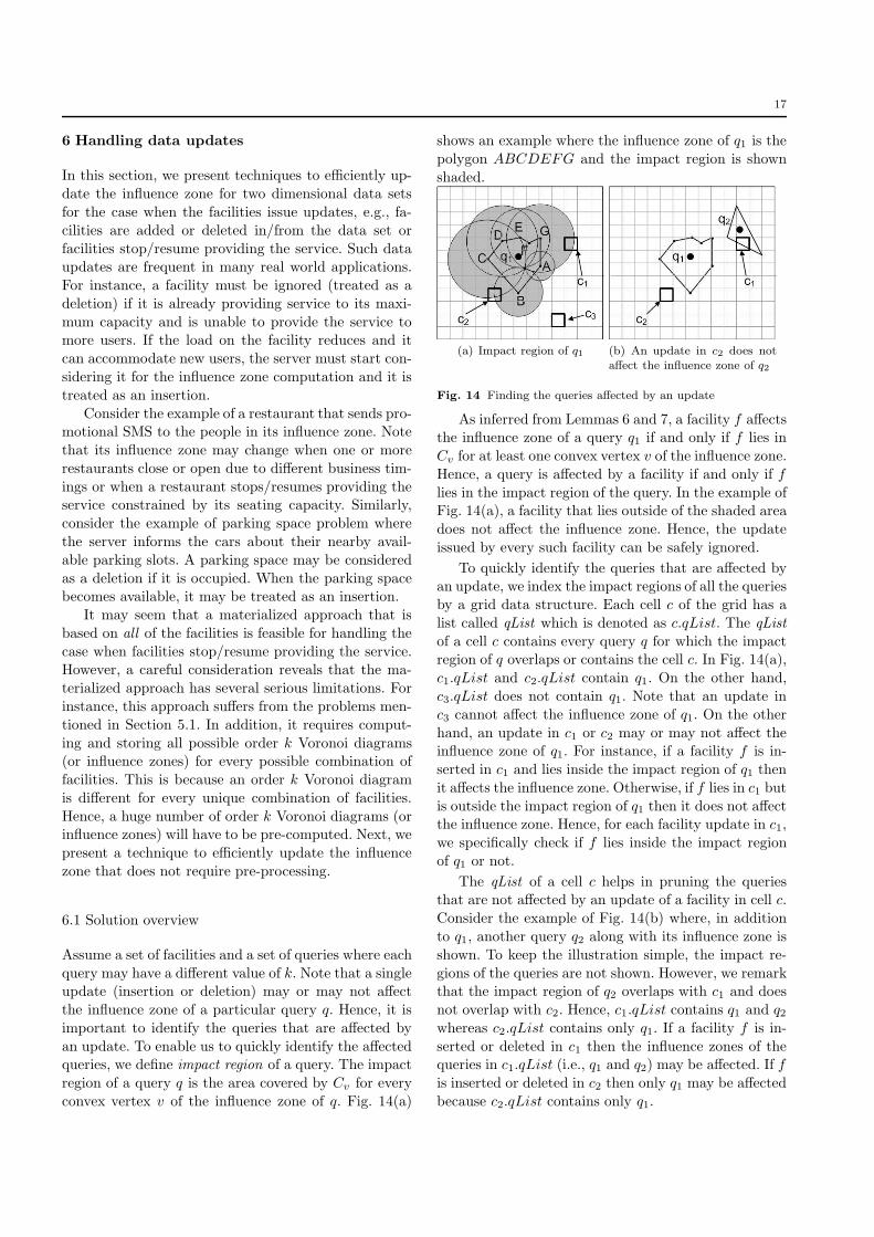
17
6 Handling data updates
In this section, we present techniques to efficiently up-
date the influence zone for two dimensional data sets
for the case when the facilities issue updates, e.g., fa-
cilities are added or deleted in/from the data set or
facilities stop/resume providing the service. Such dataupdates are frequent in many real world applications.
For instance, a facility must be ignored (treated as a
deletion) if it is already providing service to its maxi-
mum capacity and is unable to provide the service tomore users. If the load on the facility reduces and it
can accommodate new users, the server must start con-
sidering it for the influence zone computation and it is
treated as an insertion.
Consider the example of a restaurant that sends pro-motional SMS to the people in its influence zone. Note
that its influence zone may change when one or more
restaurants close or open due to different business tim-
ings or when a restaurant stops/resumes providing theservice constrained by its seating capacity. Similarly,
consider the example of parking space problem where
the server informs the cars about their nearby avail-
able parking slots. A parking space may be considered
as a deletion if it is occupied. When the parking spacebecomes available, it may be treated as an insertion.
It may seem that a materialized approach that is
based on all of the facilities is feasible for handling the
case when facilities stop/resume providing the service.However, a careful consideration reveals that the ma-
terialized approach has several serious limitations. For
instance, this approach suffers from the problems men-
tioned in Section 5.1. In addition, it requires comput-
ing and storing all possible order k Voronoi diagrams(or influence zones) for every possible combination of
facilities. This is because an order k Voronoi diagram
is different for every unique combination of facilities.
Hence, a huge number of order k Voronoi diagrams (orinfluence zones) will have to be pre-computed. Next, we
present a technique to efficiently update the influence
zone that does not require pre-processing.
6.1 Solution overview
Assume a set of facilities and a set of queries where each
query may have a different value of k. Note that a singleupdate (insertion or deletion) may or may not affect
the influence zone of a particular query q. Hence, it is
important to identify the queries that are affected by
an update. To enable us to quickly identify the affectedqueries, we define impact region of a query. The impact
region of a query q is the area covered by Cv for every
convex vertex v of the influence zone of q. Fig. 14(a)
shows an example where the influence zone of q1 is the
polygon ABCDEFG and the impact region is shown
shaded.
(a) Impact region of q1 (b) An update in c2 does notaffect the influence zone of q2
Fig. 14 Finding the queries affected by an update
As inferred from Lemmas 6 and 7, a facility f affectsthe influence zone of a query q1 if and only if f lies in
Cv for at least one convex vertex v of the influence zone.
Hence, a query is affected by a facility if and only if f
lies in the impact region of the query. In the example ofFig. 14(a), a facility that lies outside of the shaded area
does not affect the influence zone. Hence, the update
issued by every such facility can be safely ignored.
To quickly identify the queries that are affected byan update, we index the impact regions of all the queries
by a grid data structure. Each cell c of the grid has a
list called qList which is denoted as c.qList. The qList
of a cell c contains every query q for which the impactregion of q overlaps or contains the cell c. In Fig. 14(a),
c1.qList and c2.qList contain q1. On the other hand,
c3.qList does not contain q1. Note that an update in
c3 cannot affect the influence zone of q1. On the other
hand, an update in c1 or c2 may or may not affect theinfluence zone of q1. For instance, if a facility f is in-
serted in c1 and lies inside the impact region of q1 then
it affects the influence zone. Otherwise, if f lies in c1 but
is outside the impact region of q1 then it does not affectthe influence zone. Hence, for each facility update in c1,
we specifically check if f lies inside the impact region
of q1 or not.
The qList of a cell c helps in pruning the queriesthat are not affected by an update of a facility in cell c.
Consider the example of Fig. 14(b) where, in addition
to q1, another query q2 along with its influence zone is
shown. To keep the illustration simple, the impact re-
gions of the queries are not shown. However, we remarkthat the impact region of q2 overlaps with c1 and does
not overlap with c2. Hence, c1.qList contains q1 and q2whereas c2.qList contains only q1. If a facility f is in-
serted or deleted in c1 then the influence zones of thequeries in c1.qList (i.e., q1 and q2) may be affected. If f
is inserted or deleted in c2 then only q1 may be affected
because c2.qList contains only q1.
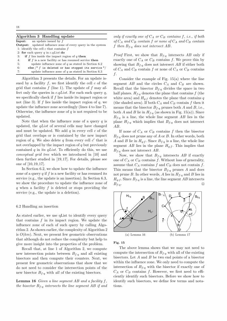
18
Algorithm 3 Handling updateInput: an update issued by fOutput: updated influence zone of every query in the system1: identify the cell c that contains f2: for each query q in c.qList do3: if f lies inside the impact region of q then
4: if f is a new facility or has resumed service then
5: update influence zone of q as stated in Section 6.26: else /* f is deleted or has stopped its service */7: update influence zone of q as stated in Section 6.3
Algorithm 3 presents the details. For an update is-
sued by a facility f , we first identify the cell c of thegrid that contains f (line 1). The update of f may af-
fect only the queries in c.qList. For each such query q,
we specifically check if f lies inside its impact region or
not (line 3). If f lies inside the impact region of q, we
update the influence zone accordingly (lines 4 to line 7).Otherwise, the influence zone of q is not required to be
updated.
Note that when the influence zone of a query q is
updated, the qList of several cells may have changed
and must be updated. We add q in every cell c of the
grid that overlaps or is contained by the new impactregion of q. We also delete q from every cell c′ that is
not overlapped by the impact region of q but previously
contained q in its qList. To efficiently do this, we use
conceptual grid tree which we introduced in [10] andthen further studied in [19,17]. For details, please see
one of [10,19,17].
In Section 6.2, we show how to update the influence
zone of a query q if f is a new facility or has resumed its
service (e.g., the update is an insertion). In Section 6.3,
we show the procedure to update the influence zone ofq when a facility f is deleted or stops providing the
service (e.g., the update is a deletion).
6.2 Handling an insertion
As stated earlier, we use qList to identify every query
that contains f in its impact region. We update the
influence zone of each of such query by calling Algo-
rithm 2. As shown earlier, the complexity of Algorithm 2is O(km). Next, we present few geometric observations
that although do not reduce the complexity but help to
give more insight into the properties of the problem.
Recall that, at line 1 of Algorithm 2, we compute
new intersection points between Bf :q and all existing
bisectors and then compute their counters. Next, wepresent few geometric observations that show that we
do not need to consider the intersection points of the
new bisector Bf :q with all of the existing bisectors.
Lemma 16 Given a line segment AB and a facility f ,
the bisector Bf :q intersects the line segment AB if and
only if exactly one of CA or CB contains f , i.e., if both
of CA and CB contain f or none of CA and CB contain
f then Bf :q does not intersect AB.
Proof First, we show that Bf :q intersects AB only if
exactly one of CA or CB contains f . We prove this by
showing that Bf :q does not intersect AB if either both
of CA and CB contain f or none of CA or CB containsf .
Consider the example of Fig. 15(a) where the line
segment AB and the circles CA and CB are shown.
Recall that the bisector Bf :q divides the space in two
half planes. Hf :q denotes the plane that contains f (the
white area) and Hq:f denotes the plane that contains q(the shaded area). If both CA and CB contain f then it
means that the bisector Bf :q prunes both A and B, i.e.,
both A and B lie in Hf :q (as shown in Fig. 15(a)). Since
Bf :q is a line, the whole line segment AB lies in theplane Hf :q which implies that Bf :q does not intersect
AB.
If none of CA or CB contains f then the bisector
Bf :q does not prune any of A or B. In other words, both
A and B lie in Hq:f . Since Bf :q is a line, the whole line
segment AB lies in the plane Hq:f . This implies thatBf :q does not intersect AB.
Now, we show that Bf :q intersects AB if exactly
one of CA or CB contains f . Without loss of generality,
assume that CA contains f and CB does not contain f .
This means that the bisector Bf :q prunes A and doesnot prune B. In other words, A lies in Hf :q and B lies in
Hq:f . Since Bf :q is a line, the line segment AB intersects
Bf :q. ⊓⊔
(a) Lemma 16 (b) Lemma 17
Fig. 15
The above lemma shows that we may not need to
compute the intersection of Bf :q with all of the existingbisectors. Let A and B be two end points of a bisector
within the influence zone. We only need to compute the
intersection of Bf :q with the bisector if exactly one of
CA or CB contains f . However, we first need to effi-ciently identify such bisectors. Before we show how to
identify such bisectors, we define few terms and nota-
tions.
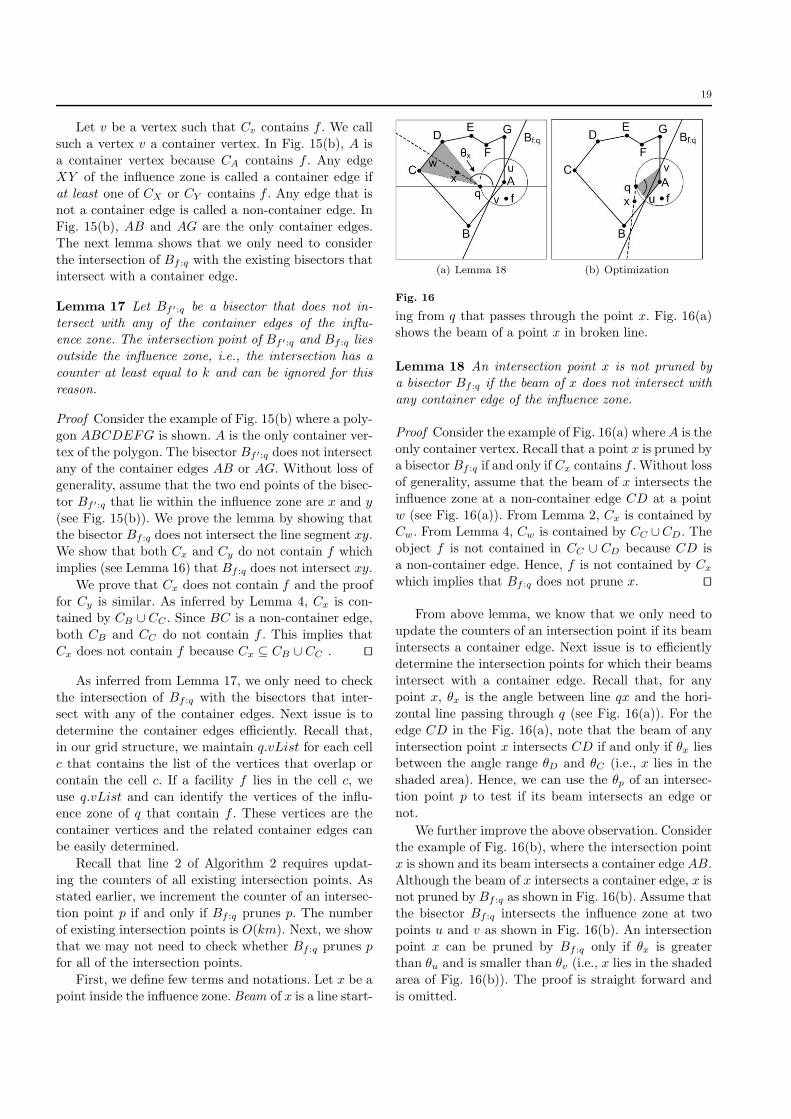
19
Let v be a vertex such that Cv contains f . We call
such a vertex v a container vertex. In Fig. 15(b), A is
a container vertex because CA contains f . Any edge
XY of the influence zone is called a container edge if
at least one of CX or CY contains f . Any edge that isnot a container edge is called a non-container edge. In
Fig. 15(b), AB and AG are the only container edges.
The next lemma shows that we only need to consider
the intersection of Bf :q with the existing bisectors thatintersect with a container edge.
Lemma 17 Let Bf ′:q be a bisector that does not in-
tersect with any of the container edges of the influ-ence zone. The intersection point of Bf ′:q and Bf :q lies
outside the influence zone, i.e., the intersection has a
counter at least equal to k and can be ignored for this
reason.
Proof Consider the example of Fig. 15(b) where a poly-
gon ABCDEFG is shown. A is the only container ver-
tex of the polygon. The bisector Bf ′:q does not intersectany of the container edges AB or AG. Without loss of
generality, assume that the two end points of the bisec-
tor Bf ′:q that lie within the influence zone are x and y
(see Fig. 15(b)). We prove the lemma by showing thatthe bisector Bf :q does not intersect the line segment xy.
We show that both Cx and Cy do not contain f which
implies (see Lemma 16) that Bf :q does not intersect xy.
We prove that Cx does not contain f and the proof
for Cy is similar. As inferred by Lemma 4, Cx is con-tained by CB ∪ CC . Since BC is a non-container edge,
both CB and CC do not contain f . This implies that
Cx does not contain f because Cx ⊆ CB ∪CC . ⊓⊔
As inferred from Lemma 17, we only need to check
the intersection of Bf :q with the bisectors that inter-
sect with any of the container edges. Next issue is to
determine the container edges efficiently. Recall that,in our grid structure, we maintain q.vList for each cell
c that contains the list of the vertices that overlap or
contain the cell c. If a facility f lies in the cell c, we
use q.vList and can identify the vertices of the influ-ence zone of q that contain f . These vertices are the
container vertices and the related container edges can
be easily determined.
Recall that line 2 of Algorithm 2 requires updat-
ing the counters of all existing intersection points. Asstated earlier, we increment the counter of an intersec-
tion point p if and only if Bf :q prunes p. The number
of existing intersection points is O(km). Next, we show
that we may not need to check whether Bf :q prunes pfor all of the intersection points.
First, we define few terms and notations. Let x be a
point inside the influence zone. Beam of x is a line start-
(a) Lemma 18 (b) Optimization
Fig. 16
ing from q that passes through the point x. Fig. 16(a)shows the beam of a point x in broken line.
Lemma 18 An intersection point x is not pruned bya bisector Bf :q if the beam of x does not intersect with
any container edge of the influence zone.
Proof Consider the example of Fig. 16(a) whereA is the
only container vertex. Recall that a point x is pruned bya bisectorBf :q if and only if Cx contains f . Without loss
of generality, assume that the beam of x intersects the
influence zone at a non-container edge CD at a point
w (see Fig. 16(a)). From Lemma 2, Cx is contained byCw. From Lemma 4, Cw is contained by CC ∪CD. The
object f is not contained in CC ∪ CD because CD is
a non-container edge. Hence, f is not contained by Cx
which implies that Bf :q does not prune x. ⊓⊔
From above lemma, we know that we only need to
update the counters of an intersection point if its beam
intersects a container edge. Next issue is to efficiently
determine the intersection points for which their beamsintersect with a container edge. Recall that, for any
point x, �x is the angle between line qx and the hori-
zontal line passing through q (see Fig. 16(a)). For the
edge CD in the Fig. 16(a), note that the beam of any
intersection point x intersects CD if and only if �x liesbetween the angle range �D and �C (i.e., x lies in the
shaded area). Hence, we can use the �p of an intersec-
tion point p to test if its beam intersects an edge or
not.
We further improve the above observation. Consider
the example of Fig. 16(b), where the intersection point
x is shown and its beam intersects a container edge AB.
Although the beam of x intersects a container edge, x isnot pruned by Bf :q as shown in Fig. 16(b). Assume that
the bisector Bf :q intersects the influence zone at two
points u and v as shown in Fig. 16(b). An intersection
point x can be pruned by Bf :q only if �x is greaterthan �u and is smaller than �v (i.e., x lies in the shaded
area of Fig. 16(b)). The proof is straight forward and
is omitted.
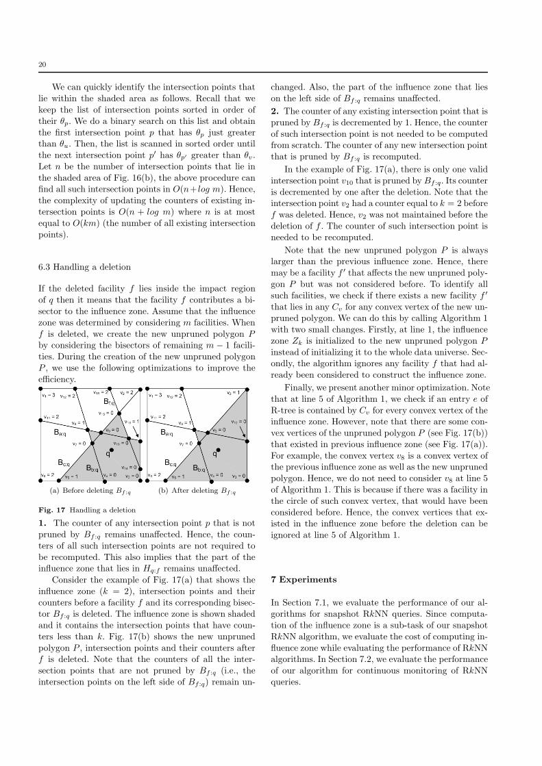
20
We can quickly identify the intersection points that
lie within the shaded area as follows. Recall that we
keep the list of intersection points sorted in order of
their �p. We do a binary search on this list and obtain
the first intersection point p that has �p just greaterthan �u. Then, the list is scanned in sorted order until
the next intersection point p′ has �p′ greater than �v.
Let n be the number of intersection points that lie in
the shaded area of Fig. 16(b), the above procedure canfind all such intersection points in O(n+ log m). Hence,
the complexity of updating the counters of existing in-
tersection points is O(n + log m) where n is at most
equal to O(km) (the number of all existing intersection
points).
6.3 Handling a deletion
If the deleted facility f lies inside the impact region
of q then it means that the facility f contributes a bi-
sector to the influence zone. Assume that the influence
zone was determined by considering m facilities. When
f is deleted, we create the new unpruned polygon Pby considering the bisectors of remaining m − 1 facili-
ties. During the creation of the new unpruned polygon
P , we use the following optimizations to improve the
efficiency.
(a) Before deleting Bf :q (b) After deleting Bf :q
Fig. 17 Handling a deletion
1. The counter of any intersection point p that is not
pruned by Bf :q remains unaffected. Hence, the coun-
ters of all such intersection points are not required to
be recomputed. This also implies that the part of theinfluence zone that lies in Hq:f remains unaffected.
Consider the example of Fig. 17(a) that shows the
influence zone (k = 2), intersection points and their
counters before a facility f and its corresponding bisec-tor Bf :q is deleted. The influence zone is shown shaded
and it contains the intersection points that have coun-
ters less than k. Fig. 17(b) shows the new unpruned
polygon P , intersection points and their counters afterf is deleted. Note that the counters of all the inter-
section points that are not pruned by Bf :q (i.e., the
intersection points on the left side of Bf :q) remain un-
changed. Also, the part of the influence zone that lies
on the left side of Bf :q remains unaffected.
2. The counter of any existing intersection point that is
pruned by Bf :q is decremented by 1. Hence, the counter
of such intersection point is not needed to be computedfrom scratch. The counter of any new intersection point
that is pruned by Bf :q is recomputed.
In the example of Fig. 17(a), there is only one valid
intersection point v10 that is pruned by Bf :q. Its counter
is decremented by one after the deletion. Note that theintersection point v2 had a counter equal to k = 2 before
f was deleted. Hence, v2 was not maintained before the
deletion of f . The counter of such intersection point is
needed to be recomputed.
Note that the new unpruned polygon P is alwayslarger than the previous influence zone. Hence, there
may be a facility f ′ that affects the new unpruned poly-
gon P but was not considered before. To identify all
such facilities, we check if there exists a new facility f ′
that lies in any Cv for any convex vertex of the new un-pruned polygon. We can do this by calling Algorithm 1
with two small changes. Firstly, at line 1, the influence
zone Zk is initialized to the new unpruned polygon P
instead of initializing it to the whole data universe. Sec-ondly, the algorithm ignores any facility f that had al-
ready been considered to construct the influence zone.
Finally, we present another minor optimization. Note
that at line 5 of Algorithm 1, we check if an entry e of
R-tree is contained by Cv for every convex vertex of theinfluence zone. However, note that there are some con-
vex vertices of the unpruned polygon P (see Fig. 17(b))
that existed in previous influence zone (see Fig. 17(a)).
For example, the convex vertex v8 is a convex vertex ofthe previous influence zone as well as the new unpruned
polygon. Hence, we do not need to consider v8 at line 5
of Algorithm 1. This is because if there was a facility in
the circle of such convex vertex, that would have been
considered before. Hence, the convex vertices that ex-isted in the influence zone before the deletion can be
ignored at line 5 of Algorithm 1.
7 Experiments
In Section 7.1, we evaluate the performance of our al-gorithms for snapshot RkNN queries. Since computa-
tion of the influence zone is a sub-task of our snapshot
RkNN algorithm, we evaluate the cost of computing in-
fluence zone while evaluating the performance of RkNNalgorithms. In Section 7.2, we evaluate the performance
of our algorithm for continuous monitoring of RkNN
queries.
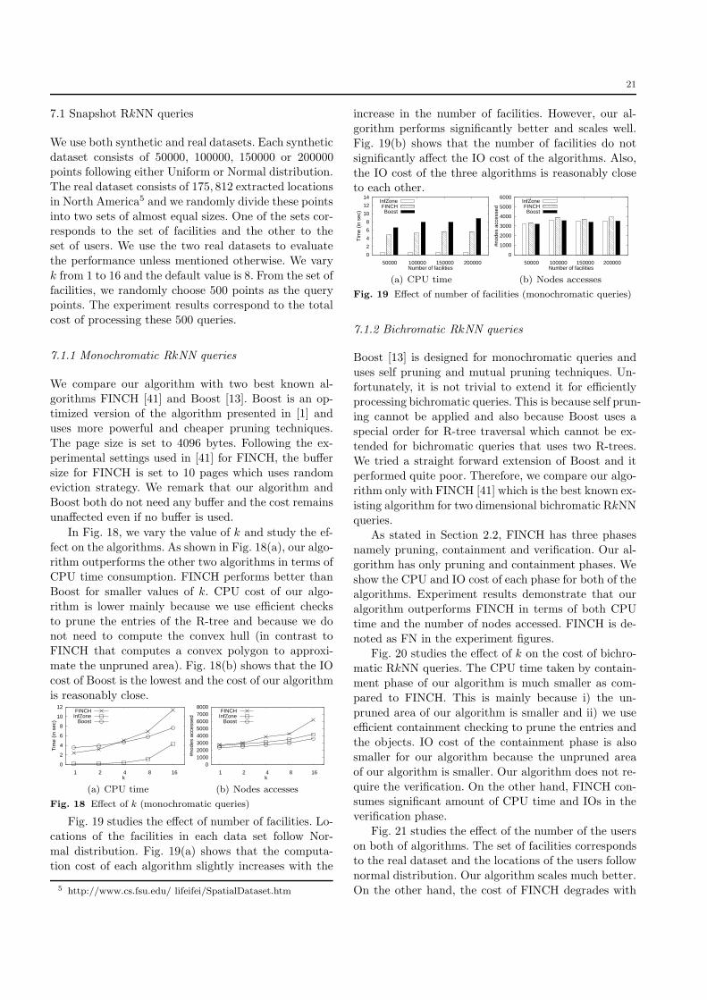
21
7.1 Snapshot RkNN queries
We use both synthetic and real datasets. Each synthetic
dataset consists of 50000, 100000, 150000 or 200000points following either Uniform or Normal distribution.
The real dataset consists of 175, 812 extracted locations
in North America5 and we randomly divide these points
into two sets of almost equal sizes. One of the sets cor-responds to the set of facilities and the other to the
set of users. We use the two real datasets to evaluate
the performance unless mentioned otherwise. We vary
k from 1 to 16 and the default value is 8. From the set of
facilities, we randomly choose 500 points as the querypoints. The experiment results correspond to the total
cost of processing these 500 queries.
7.1.1 Monochromatic RkNN queries
We compare our algorithm with two best known al-
gorithms FINCH [41] and Boost [13]. Boost is an op-timized version of the algorithm presented in [1] and
uses more powerful and cheaper pruning techniques.
The page size is set to 4096 bytes. Following the ex-
perimental settings used in [41] for FINCH, the buffer
size for FINCH is set to 10 pages which uses randomeviction strategy. We remark that our algorithm and
Boost both do not need any buffer and the cost remains
unaffected even if no buffer is used.
In Fig. 18, we vary the value of k and study the ef-
fect on the algorithms. As shown in Fig. 18(a), our algo-
rithm outperforms the other two algorithms in terms ofCPU time consumption. FINCH performs better than
Boost for smaller values of k. CPU cost of our algo-
rithm is lower mainly because we use efficient checks
to prune the entries of the R-tree and because we donot need to compute the convex hull (in contrast to
FINCH that computes a convex polygon to approxi-
mate the unpruned area). Fig. 18(b) shows that the IO
cost of Boost is the lowest and the cost of our algorithm
is reasonably close.
0
2
4
6
8
10
12
1 2 4 8 16
Tim
e (in
sec
)
k
FINCHInfZone
Boost
(a) CPU time
0 1000 2000 3000 4000 5000 6000 7000 8000
1 2 4 8 16
#nod
es a
cces
sed
k
FINCHInfZone
Boost
(b) Nodes accesses
Fig. 18 Effect of k (monochromatic queries)
Fig. 19 studies the effect of number of facilities. Lo-
cations of the facilities in each data set follow Nor-
mal distribution. Fig. 19(a) shows that the computa-
tion cost of each algorithm slightly increases with the
5 http://www.cs.fsu.edu/ lifeifei/SpatialDataset.htm
increase in the number of facilities. However, our al-
gorithm performs significantly better and scales well.
Fig. 19(b) shows that the number of facilities do not
significantly affect the IO cost of the algorithms. Also,
the IO cost of the three algorithms is reasonably closeto each other.
0
2
4
6
8
10
12
14
50000 100000 150000 200000
Tim
e (in
sec
)
Number of facilities
InfZoneFINCHBoost
(a) CPU time
0
1000
2000
3000
4000
5000
6000
50000 100000 150000 200000
#nod
es a
cces
sed
Number of facilities
InfZoneFINCHBoost
(b) Nodes accesses
Fig. 19 Effect of number of facilities (monochromatic queries)
7.1.2 Bichromatic RkNN queries
Boost [13] is designed for monochromatic queries and
uses self pruning and mutual pruning techniques. Un-
fortunately, it is not trivial to extend it for efficientlyprocessing bichromatic queries. This is because self prun-
ing cannot be applied and also because Boost uses a
special order for R-tree traversal which cannot be ex-
tended for bichromatic queries that uses two R-trees.We tried a straight forward extension of Boost and it
performed quite poor. Therefore, we compare our algo-
rithm only with FINCH [41] which is the best known ex-
isting algorithm for two dimensional bichromatic RkNN
queries.As stated in Section 2.2, FINCH has three phases
namely pruning, containment and verification. Our al-
gorithm has only pruning and containment phases. We
show the CPU and IO cost of each phase for both of thealgorithms. Experiment results demonstrate that our
algorithm outperforms FINCH in terms of both CPU
time and the number of nodes accessed. FINCH is de-
noted as FN in the experiment figures.
Fig. 20 studies the effect of k on the cost of bichro-matic RkNN queries. The CPU time taken by contain-
ment phase of our algorithm is much smaller as com-
pared to FINCH. This is mainly because i) the un-
pruned area of our algorithm is smaller and ii) we useefficient containment checking to prune the entries and
the objects. IO cost of the containment phase is also
smaller for our algorithm because the unpruned area
of our algorithm is smaller. Our algorithm does not re-
quire the verification. On the other hand, FINCH con-sumes significant amount of CPU time and IOs in the
verification phase.
Fig. 21 studies the effect of the number of the users
on both of algorithms. The set of facilities correspondsto the real dataset and the locations of the users follow
normal distribution. Our algorithm scales much better.
On the other hand, the cost of FINCH degrades with
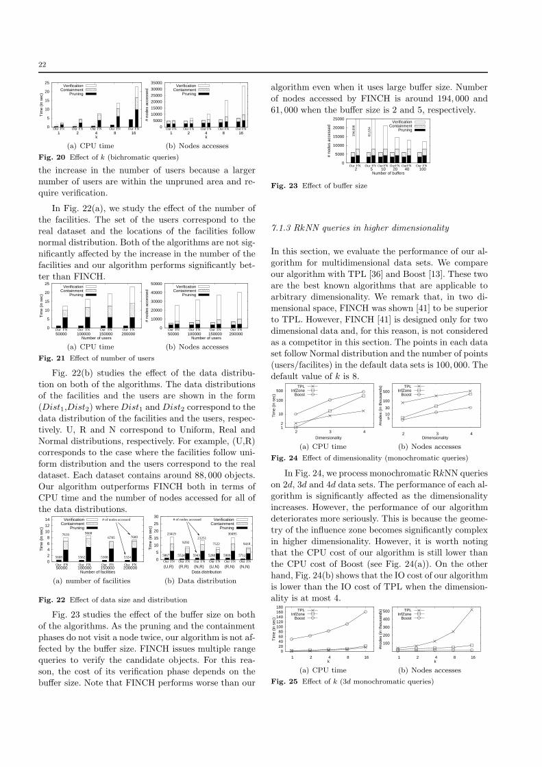
22
0
5
10
15
20
25
1 2 4 8 16
Tim
e (in
sec
)
k
Our Our Our Our OurFN FN FN FN FN
VerificationContainment
Pruning
(a) CPU time
0
5000
10000
15000
20000
25000
30000
35000
1 2 4 8 16
# no
des
acce
ssed
k
Our Our Our Our OurFN FN FN FN FN
VerificationContainment
Pruning
(b) Nodes accesses
Fig. 20 Effect of k (bichromatic queries)
the increase in the number of users because a larger
number of users are within the unpruned area and re-quire verification.
In Fig. 22(a), we study the effect of the number of
the facilities. The set of the users correspond to the
real dataset and the locations of the facilities follownormal distribution. Both of the algorithms are not sig-
nificantly affected by the increase in the number of the
facilities and our algorithm performs significantly bet-
ter than FINCH.
0
5
10
15
20
25
50000 100000 150000 200000
Tim
e (in
sec
)
Number of users
Our Our Our OurFN FN FN FN
VerificationContainment
Pruning
(a) CPU time
0
10000
20000
30000
40000
50000
50000 100000 150000 200000
# no
des
acce
ssed
Number of users
Our Our Our OurFN FN FN FN
VerificationContainment
Pruning
(b) Nodes accesses
Fig. 21 Effect of number of users
Fig. 22(b) studies the effect of the data distribu-
tion on both of the algorithms. The data distributionsof the facilities and the users are shown in the form
(Dist1,Dist2) whereDist1 and Dist2 correspond to the
data distribution of the facilities and the users, respec-
tively. U, R and N correspond to Uniform, Real and
Normal distributions, respectively. For example, (U,R)corresponds to the case where the facilities follow uni-
form distribution and the users correspond to the real
dataset. Each dataset contains around 88, 000 objects.
Our algorithm outperforms FINCH both in terms ofCPU time and the number of nodes accessed for all of
the data distributions.
0
2
4
6
8
10
12
14
50000 100000 150000 200000
Tim
e (in
sec
)
Number of facilities
Our Our Our OurFN FN FN FN
5608 5562 5308 5324
7619 96686785 7600
# of nodes accessedVerificationContainment
Pruning
(a) number of facilities
0
5
10
15
20
25
30
(U,R) (R,R) (N,R) (U,N) (R,N) (N,N)
Tim
e (in
sec
)
Data distribution
Our Our Our Our Our OurFN FN FN FN FN FN
5867 5524 5943 5288 5989 5711
23419
929221251
7522
30495
9418
# of nodes accessed VerificationContainment
Pruning
(b) Data distribution
Fig. 22 Effect of data size and distribution
Fig. 23 studies the effect of the buffer size on both
of the algorithms. As the pruning and the containment
phases do not visit a node twice, our algorithm is not af-
fected by the buffer size. FINCH issues multiple rangequeries to verify the candidate objects. For this rea-
son, the cost of its verification phase depends on the
buffer size. Note that FINCH performs worse than our
algorithm even when it uses large buffer size. Number
of nodes accessed by FINCH is around 194, 000 and
61, 000 when the buffer size is 2 and 5, respectively.
0
5000
10000
15000
20000
25000
2 5 10 20 40 100
# no
des
acce
ssed
Number of buffers
Our Our Our Our Our OurFN FN FN FN FN FN
194,
698
61,6
34
VerificationContainment
Pruning
Fig. 23 Effect of buffer size
7.1.3 RkNN queries in higher dimensionality
In this section, we evaluate the performance of our al-
gorithm for multidimensional data sets. We compare
our algorithm with TPL [36] and Boost [13]. These two
are the best known algorithms that are applicable to
arbitrary dimensionality. We remark that, in two di-mensional space, FINCH was shown [41] to be superior
to TPL. However, FINCH [41] is designed only for two
dimensional data and, for this reason, is not considered
as a competitor in this section. The points in each dataset follow Normal distribution and the number of points
(users/facilites) in the default data sets is 100, 000. The
default value of k is 8.
1 2
10
100
500
2 3 4
Tim
e (in
sec
)
Dimensionality
TPLInfZone
Boost
(a) CPU time
510
30
100
500
2 3 4
#nod
es (
in th
ousa
nds)
Dimensionality
TPLInfZone
Boost
(b) Nodes accesses
Fig. 24 Effect of dimensionality (monochromatic queries)
In Fig. 24, we process monochromatic RkNN queries
on 2d, 3d and 4d data sets. The performance of each al-gorithm is significantly affected as the dimensionality
increases. However, the performance of our algorithm
deteriorates more seriously. This is because the geome-
try of the influence zone becomes significantly complex
in higher dimensionality. However, it is worth notingthat the CPU cost of our algorithm is still lower than
the CPU cost of Boost (see Fig. 24(a)). On the other
hand, Fig. 24(b) shows that the IO cost of our algorithm
is lower than the IO cost of TPL when the dimension-ality is at most 4.
0 20 40 60 80
100 120 140 160 180
1 2 4 8 16
Tim
e (in
sec
)
k
TPLInfZone
Boost
(a) CPU time
100
200
300
400
500
1 2 4 8 16
#nod
es (
in th
ousa
nds)
k
TPLInfZone
Boost
(b) Nodes accesses
Fig. 25 Effect of k (3d monochromatic queries)
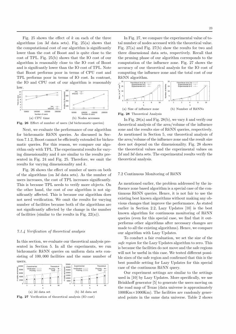
23
Fig. 25 shows the effect of k on each of the three
algorithms (on 3d data sets). Fig. 25(a) shows that
the computational cost of our algorithm is significantly
lower than the cost of Boost and is quite close to the
cost of TPL. Fig. 25(b) shows that the IO cost of ouralgorithm is reasonably close to the IO cost of Boost
and is signifcantly lower than the IO cost of TPL. Note
that Boost performs poor in terms of CPU cost and
TPL performs poor in terms of IO cost. In contrast,the IO and CPU cost of our algorithm is reasonably
low.
0
2
4
6
8
10
12
14
50000 100000 150000 200000
Tim
e (in
sec
)
Number of users
TPLInfZone
(a) CPU time
100
200
300
400
50000 100000 150000 200000
#nod
es (
in th
ousa
nds)
Number of users
TPLInfZone
(b) Nodes accesses
Fig. 26 Effect of number of users (3d bichromatic queries)
Next, we evaluate the performance of our algorithm
for bichromatic RkNN queries. As discussed in Sec-
tion 7.1.2, Boost cannot be efficiently extended for bichro-matic queries. For this reason, we compare our algo-
rithm only with TPL. The experimental results for vary-
ing dimensionality and k are similar to the results pre-
sented in Fig. 24 and Fig. 25. Therefore, we omit theresults for varying dimensionality and k.
Fig. 26 shows the effect of number of users on both
of the algorithms (on 3d data sets). As the number of
users increases, the cost of TPL increases significantly.
This is because TPL needs to verify more objects. On
the other hand, the cost of our algorithm is not sig-nificantly affected. This is because our algorithm does
not need verification. We omit the results for varying
number of facilities because both of the algorithms are
not significantly affected by the change in the numberof facilities (similar to the results in Fig. 22(a)).
7.1.4 Verification of theoretical analysis
In this section, we evaluate our theoretical analysis pre-
sented in Section 5. In all the experiments, we run
bichromatic RkNN queries on uniform data sets con-
sisting of 100, 000 facilities and the same number of
users.
0
2000
4000
6000
8000
10000
1 2 4 8 16
# no
des
acce
ssed
k
Experimental TheoreticalVerification
PruningPruning
Total
(a) 2d data set
0
5000
10000
15000
20000
25000
30000
35000
1 2 4 8 16
# no
des
acce
ssed
k
Experimental TheoreticalVerification
PruningPruning
Total
(b) 3d data set
Fig. 27 Verification of theoretical analysis (IO cost)
In Fig. 27, we compare the experimental value of to-
tal number of nodes accessed with the theoretical value.
Fig. 27(a) and Fig. 27(b) show the results for two and
three dimensional data sets, respectively. Recall that
the pruning phase of our algorithm corresponds to thecomputation of the influence zone. Fig. 27 shows the
accuracy of our theoretical analysis for the IO cost of
computing the influence zone and the total cost of our
RkNN algorithm.
0
5
10
15
20
1 2 4 8 16
Siz
e (
in 1
0-5 u
nits
d )
k
Theoretical 2d & 3dExperimental d=2Experimental d=3
(a) Size of influence zone
0
5
10
15
20
1 2 4 8 16
Num
ber
of R
kNN
s
k
Theoretical 2d & 3dExperimental d=2Experimental d=3
(b) Number of RkNNs
Fig. 28 Theoretical Analysis
In Fig. 28(a) and Fig. 28(b), we vary k and verify our
theoretical analysis of the area/volume of the influencezone and the results size of RkNN queries, respectively.
As mentioned in Section 5, our theoretical analysis of
the area/volume of the influence zone and the result size
does not depend on the dimensionality. Fig. 28 showsthe theoretical values and the experimental values on
2d and 3d data sets. The experimental results verify the
theoretical analysis.
7.2 Continuous Monitoring of RkNN
As mentioned earlier, the problem addressed by the in-
fluence zone based algorithm is a special case of the con-
tinuous RkNN queries. Hence, it is not fair to use the
existing best known algorithms without making any ob-
vious changes that improve the performance. As statedearlier in Section 2.2, Lazy Updates [10] is the best
known algorithm for continuous monitoring of RkNN
queries (even for this special case, we find that it out-
performs other algorithms after necessary changes aremade to all the existing algorithms). Hence, we compare
our algorithm with Lazy Updates.
To conduct a fair evaluation, we set the size of the
safe region for the Lazy Updates algorithm to zero. This
is because the facilities do not move and the safe regions
will not be useful in this case. We tested different possi-ble sizes of the safe region and confirmed that this is the
best possible setting for Lazy Updates for this special
case of the continuous RkNN query.
Our experiment settings are similar to the settings
used in [10] by Lazy Updates. More specifically, we use
Brinkhoff generator [5] to generate the users moving onthe road map of Texas (data universe is approximately
1000Km×1000Km). The facilities are randomly gener-
ated points in the same data universe. Table 2 shows
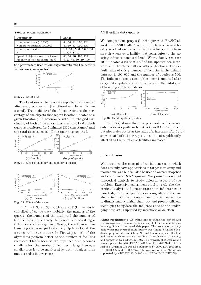
24
Table 2 System Parameters
Parameter Range
Number of users (×1000) 40, 60, 80, 100, 120
Number of facilities (×1000) 40, 60, 80, 100, 120
Number of queries 100, 300, 500, 700, 1000
k 1, 2, 4, 8, 16
Speed of objects (users) in km/ℎr 40, 60, 80, 100, 120
Mobility of objects (users) in % 5, 20, 40, 60, 80, 100
the parameters used in our experiments and the defaultvalues are shown in bold.
0
50
100
150
200
250
300
1 2 4 8 16
Tim
e (s
econ
ds)
k
LazyUpdatesInfZone
Fig. 29 Effect of k
The locations of the users are reported to the server
after every one second (i.e., timestamp length is one
second). The mobility of the objects refers to the per-
centage of the objects that report location updates at agiven timestamp. In accordance with [10], the grid car-
dinality of both of the algorithms is set to 64×64. Each
query is monitored for 5 minutes (300 timestamps) and
the total time taken by all the queries is reported.
0
20
40
60
80
100
120
140
5 20 40 60 80 100
Tim
e (in
sec
)
Mobility (in %)
LazyUpdatesInfZone
(a) Mobility
0
50
100
150
200
250
100 300 500 700 1000
Tim
e (s
econ
ds)
Number of queries
LazyUpdatesInfZone
(b) # of queries
Fig. 30 Effect of mobility and number of queries
0
20
40
60
80
100
120
140
40 60 80 100 120
Tim
e (s
econ
ds)
Number of users (in thousands)
LazyUpdatesInfZone
(a) # of users
0 20 40 60 80
100 120 140 160 180 200
40 60 80 100 120
Tim
e (in
sec
)
Number of Facilities (in thousands)
LazyUpdatesInfZone
(b) # of facilities
Fig. 31 Effect of data size
In Fig. 29, 30(a), 30(b), 31(a) and 31(b), we study
the effect of k, the data mobility, the number of the
queries, the number of the users and the number of
the facilities, respectively. Influence zone based algo-
rithm is shown as InfZone. Clearly, the influence zonebased algorithm outperforms Lazy Updates for all the
settings and scales better. In Fig. 31(b), both of the
algorithms perform better as the number of facilities
increases. This is because the unpruned area becomessmaller when the number of facilities is large. Hence, a
smaller area is to be monitored by both the algorithms
and it results in lower cost.
7.3 Handling data updates
We compare our proposed technique with BASIC al-
gorithm. BASIC calls Algorithm 2 whenever a new fa-cility is added and recomputes the influence zone from
scratch whenever a facility that contributes to the ex-
isting influence zone is deleted. We randomly generate
1000 updates such that half of the updates are inser-
tions and the other half consists of deletions. The de-fault value of k is 8, number of facilities in the default
data set is 100, 000 and the number of queries is 500.
The influence zone of each of the query is updated after
every data update and the results show the total costof handling all data updates.
0
5
10
15
20
25
30
35
1 2 4 8 16
Tim
e (s
econ
ds)
k
BasicOUR
(a) effect of k
0
5
10
15
20
25
50000 100000 150000 200000
Tim
e (s
econ
ds)
number of facilities
BasicOUR
(b) # of facilities
Fig. 32 Handling data updates
Fig. 32(a) shows that our proposed technique notonly performs significantly better than BASIC approach
but also scales better as the value of k increases. Fig. 32(b)
shows that both of the algorithms are not significantly
affected as the number of facilities increases.
8 Conclusion
We introduce the concept of an influence zone which
does not only have applications in target marketing andmarket analysis but can also be used to answer snapshot
and continuous RkNN queries. We present a detailed
theoretical analysis to study different aspects of the
problem. Extensive experiment results verify the the-oretical analysis and demonstrate that influence zone
based algorithm outperforms existing algorithms. We
also extend our technique to compute influence zone
in dimensionality higher than two. and present efficient
techniques to update the influence zone as the under-lying data set is updated by insertions or deletion.
Acknowledgements We would like to thank the editors andthe anonymous reviewers for their very helpful comments thathave significantly improved this paper. The work was partiallydone when the corresponding author was taking a Chinese aca-demic program at East China Normal University; and the firstand second authors were visiting East China Normal University,and supported by NSFC61021004. The research of Wenjie Zhangwas supported by ARC DP120104168 and DE120102144. The re-search of Xuemin Lin was also supported by ARC DP120104168,DP110102937 and DP0987557. The research of Ying Zhang wassupported by ARC DP110104880 and UNSW ECR PSE1799.
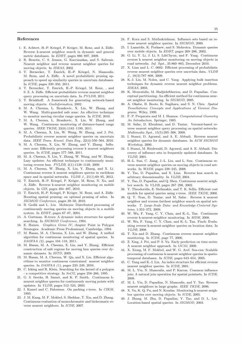
25
References
1. E. Achtert, H.-P. Kriegel, P. Kroger, M. Renz, and A. Zufle.Reverse k-nearest neighbor search in dynamic and generalmetric databases. In EDBT, pages 886–897, 2009.
2. R. Benetis, C. S. Jensen, G. Karciauskas, and S. Saltenis.Nearest neighbor and reverse nearest neighbor queries formoving objects. In IDEAS, 2002.
3. T. Bernecker, T. Emrich, H.-P. Kriegel, N. Mamoulis,M. Renz, and A. Zufle. A novel probabilistic pruning ap-proach to speed up similarity queries in uncertain databases.In ICDE, pages 339–350, 2011.
4. T. Bernecker, T. Emrich, H.-P. Kriegel, M. Renz, , andS. Z. A. Zufle. Efficient probabilistic reverse nearest neighborquery processing on uncertain data. In PVLDB, 2011.
5. T. Brinkhoff. A framework for generating network-basedmoving objects. GeoInformatica, 2002.
6. M. A. Cheema, L. Brankovic, X. Lin, W. Zhang, andW. Wang. Multi-guarded safe zone: An effective techniqueto monitor moving circular range queries. In ICDE, 2010.
7. M. A. Cheema, L. Brankovic, X. Lin, W. Zhang, andW. Wang. Continuous monitoring of distance-based rangequeries. IEEE TKDE, 23(8):1182–1199, 2011.
8. M. A. Cheema, X. Lin, W. Wang, W. Zhang, and J. Pei.
Probabilistic reverse nearest neighbor queries on uncertaindata. IEEE Trans. Knowl. Data Eng., 22(4):550–564, 2010.
9. M. A. Cheema, X. Lin, W. Zhang, and Y. Zhang. Influ-ence zone: Efficiently processing reverse k nearest neighborsqueries. In ICDE, pages 577–588, 2011.
10. M. A. Cheema, X. Lin, Y. Zhang, W. Wang, and W. Zhang.Lazy updates: An efficient technique to continuously moni-toring reverse knn. PVLDB, 2(1):1138–1149, 2009.
11. M. A. Cheema, W. Zhang, X. Lin, Y. Zhang, and X. Li.Continuous reverse k nearest neighbors queries in euclideanspace and in spatial networks. VLDB J., 21(1):69–95, 2012.
12. T. Emrich, H.-P. Kriegel, P. Kroger, M. Renz, N. Xu, andA. Zufle. Reverse k-nearest neighbor monitoring on mobileobjects. In GIS, pages 494–497, 2010.
13. T. Emrich, H.-P. Kriegel, P. Kroger, M. Renz, and A. Zufle.Boosting spatial pruning: on optimal pruning of mbrs. InSIGMOD Conference, pages 39–50, 2010.
14. B. Gedik and L. Liu. Mobieyes: Distributed processing ofcontinuously moving queries on moving objects in a mobilesystem. In EDBT, pages 67–87, 2004.
15. A. Guttman. R-trees: A dynamic index structure for spatialsearching. In SIGMOD Conference, 1984.
16. E. Haines. Graphics Gems IV, chapter Point in PolygonStrategies. Academic Press Professional, Cambridge, 1994.
17. M. Hasan, M. A. Cheema, X. Lin, and W. Zhang. A unifiedalgorithm for continuous monitoring of spatial queries. InDASFAA (2), pages 104–118, 2011.
18. M. Hasan, M. A. Cheema, X. Lin, and Y. Zhang. Efficientconstruction of safe regions for moving knn queries over dy-
namic datasets. In SSTD, 2009.19. M. Hasan, M. A. Cheema, W. Qu, and X. Lin. Efficient algo-
rithms to monitor continuous constrained nearest neighborqueries. In DASFAA (1), pages 233–249, 2010.
20. C. Icking and R. Klein. Searching for the kernel of a polygon- a competitive strategy. In SoCG, pages 258–266, 1995.
21. G. S. Iwerks, H. Samet, and K. P. Smith. Continuous k-nearest neighbor queries for continuously moving points withupdates. In VLDB, pages 512–523, 2003.
22. I. Kamel and C. Faloutsos. On packing r-trees. In CIKM,1993.
23. J. M. Kang, M. F. Mokbel, S. Shekhar, T. Xia, and D. Zhang.Continuous evaluation of monochromatic and bichromatic re-verse nearest neighbors. In ICDE, 2007.
24. F. Korn and S. Muthukrishnan. Influence sets based on re-verse nearest neighbor queries. In SIGMOD, 2000.
25. I. Lazaridis, K. Porkaew, and S. Mehrotra. Dynamic queriesover mobile objects. In EDBT, pages 269–286, 2002.
26. G. Li, Y. Li, J. Li, S. LihChyun, and F. Yang. Continuousreverse k nearest neighbor monitoring on moving objects inroad networks. Inf. Syst., 35:860–883, December 2010.
27. X. Lian and L. C. 0002. Efficient processing of probabilisticreverse nearest neighbor queries over uncertain data. VLDBJ., 18(3):787–808, 2009.
28. K.-I. Lin, M. Nolen, and C. Yang. Applying bulk insertiontechniques for dynamic reverse nearest neighbor problems.IDEAS, 2003.
29. K. Mouratidis, M. Hadjieleftheriou, and D. Papadias. Con-ceptual partitioning: An efficient method for continuous near-est neighbor monitoring. In SIGMOD, 2005.
30. A. Okabe, B. Boots, K. Sugihara, and S. N. Chiu. SpatialTessellations: Concepts and Applications of Voronoi Dia-grams. Wiley, 1999.
31. F. P. Preparata and M. I. Shamos. Computational GeometryAn Introduction. Springer, 1985.
32. M. Safar, D. Ebrahimi, and D. Taniar. Voronoi-based re-verse nearest neighbor query processing on spatial networks.Multimedia Syst., 15(5):295–308, 2009.
33. I. Stanoi, D. Agrawal, and A. E. Abbadi. Reverse nearestneighbor queries for dynamic databases. In ACM SIGMODWorkshop, 2000.
34. I. Stanoi, M. Riedewald, D. Agrawal, and A. E. Abbadi. Dis-covery of influence sets in frequently updated databases. InVLDB, 2001.
35. H.-L. Sun, C. Jiang, J.-L. Liu, and L. Sun. Continuous re-verse nearest neighbor queries on moving objects in road net-works. In WAIM, pages 238–245, 2008.
36. Y. Tao, D. Papadias, and X. Lian. Reverse knn search inarbitrary dimensionality. In VLDB, 2004.
37. Y. Tao, D. Papadias, and Q. Shen. Continuous nearest neigh-bor search. In VLDB, pages 287–298, 2002.
38. Y. Theodoridis, E. Stefanakis, and T. K. Sellis. Efficient costmodels for spatial queries using r-trees. IEEE TKDE, 2000.
39. Q. T. Tran, D. Taniar, and M. Safar. Reverse k nearestneighbor and reverse farthest neighbor search on spatial net-works. T. Large-Scale Data- and Knowledge-Centered Sys-tems, 1:353–372, 2009.
40. W. Wu, F. Yang, C. Y. Chan, and K.-L. Tan. Continuousreverse k-nearest-neighbor monitoring. In MDM, 2008.
41. W. Wu, F. Yang, C. Y. Chan, and K.-L. Tan. Finch: Evalu-ating reverse k-nearest-neighbor queries on location data. InVLDB, 2008.
42. T. Xia and D. Zhang. Continuous reverse nearest neighbormonitoring. In ICDE, page 77, 2006.
43. Z. Xing, J. Pei, and P. S. Yu. Early prediction on time series:A nearest neighbor approach. In IJCAI, 2009.
44. X. Xiong, M. F. Mokbel, and W. G. Aref. Sea-cnn: Scalableprocessing of continuous k-nearest neighbor queries in spatio-temporal databases. In ICDE, pages 643–654, 2005.
45. C. Yang and K.-I. Lin. An index structure for efficient reversenearest neighbor queries. In ICDE, 2001.
46. M. L. Yiu, N. Mamoulis, and P. Karras. Common influencejoin: A natural join operation for spatial pointsets. In ICDE,2008.
47. M. L. Yiu, D. Papadias, N. Mamoulis, and Y. Tao. Reversenearest neighbors in large graphs. IEEE TKDE, 2006.
48. X. Yu, K. Q. Pu, and N. Koudas. Monitoring k-nearest neigh-bor queries over moving objects. In ICDE, 2005.
49. J. Zhang, M. Zhu, D. Papadias, Y. Tao, and D. L. Lee.Location-based spatial queries. In SIGMOD, 2003.