Submitted to the special edition of Physical Review Special Topic Accelerator andBeam

Efficient Numerical and Parallel Methods for

Beam Dynamics Simulations

Jin Xu1,2, Brahim Mustapha1, and Misun Min2

1Physics Division2Mathematics and Computer Science Division

Argonne National Laboratory9700 S. Cass Ave., Argonne, IL 60439, USA

Abstract

Efficient numerical and parallel methods have been used at Argonne National Labora-tory (ANL) to develop petascalable software packages for beam dynamics simulations. Thispaper is an summary of the numerical methods and parallel algorithms used and developedin the past five years at ANL. It is an extension to the paper “Developing petascalablealgorithms for beam dynamics simulations,” on proceeding of the first International Parti-cle Accelerator Conference IPAC-2010 [33]. In this paper, numerical methods and parallelalgorithms for our beam dynamics simulations are summarized. These include the standardparticle-in-cell (PIC) method, direct Vlasov solvers and scalable Poisson solvers. Efficientparallel algorithms for these methods on supercomputers have been implemented and havesuccessfully used tens of thousands processors on the IBM Blue Gene/P system at theArgonne Leadership Computing Facility (ALCF). Among them, scalable Poisson solversin three dimensions, to account for space charge effects, are the most challenging. Severalmethods have been used to solve Poisson’s equation efficiently in different situations. TheALCF provides a suitable environment to perform large scale beam dynamics simulations.High-order numerical methods have been adopted to increase the accuracy. Domain de-composition methods have been used for parallelizing the solvers, and good scaling hasbeen achieved. Preliminary results for the direct Vlasov solvers have been obtained in up tofour dimensions. The parallel beam dynamics code PTRACK, which uses the PIC methodto solve Poisson’s equation, has been used as a workhorse for end-to-end simulations andlarge-scale design optimizations for linear accelerators.

Key words: Poisson’s Equation, Vlasov Equation, hp-FEM, Semi-Lagrangian Method,Discontinuous Galerkin Method, High Dimension, Multigrid Technique

PACS subject classifications: 02.60.-x; 02.70.-c; 07.05.Tp; 52.65.-y;

1 Introduction

Beam dynamics simulations (BDS) play a significant role in accelerator model-ing, they are important for both the design and operation phases of an accelerator.Computational beam dynamics have become more powerful with the development ofsupercomputers capable of simulating more complex effects and phenomena in beamphysics. As the computing era enters petascale, more accurate accelerator simulationscan be conducted. In order to efficiently use this computing power, we need to developmore efficient numerical and parallel methods. This paper introduces our efforts inthis direction that is to apply efficient numerical methods and develop scalable meth-ods necessary for large scale BDS. We explain various numerical and parallel methodsin a way that is easy to understand, and we direct the interested reader to relatedjournals for more detailed information [28,30–32]. These efforts are limited and stillon going, and there are many other efficient numerical methods not been included.We will try and report them in the future studies.

Charged particle beams are at the core of accelerator technology. Since chargedbeam is a kind of plasma, most of the methods used for plasma simulations could beadopted and used for charged beam simulations. The methods for simulating plasmacan be divided into three categories: microscopic models, kinetic models, and fluidmodels. In the microscopic model, each charged particle is described by six variables(x, y, z, vx, vy, vz). Therefore, for N particles, there are 6N variables in total. Sinceeach two particles have mutual force interaction, this leads to a group of 6N equa-tions which has 6N variables in each of them. Solving the beam dynamics equationin 6N dimensions exceeds the capability of current supercomputers for large N. Thefluid model is the simplest, because it treats the plasma as a conducting fluid withelectromagnetic forces exerted on it. This leads to solving the magnetohydrodynam-ics (MHD) equations in 3D (x, y, z); MHD techniques solve for average quantities,such as density and charge. Since charged beams are often accelerated and focusedin bunches makes the fluid model, which is successful to describe a continuous flowof fluid, not suitable for charged beam simulations. Between these two models is thekinetic model, which is used by most current beam dynamics simulations. This modelobtains the charge density function by solving the Boltzmann or Vlasov equations in6 dimensions (x, y, z, vx, vy, vz). The Vlasov equation describes the evolution of a sys-tem of particles under the effects of self-consistent electromagnetic fields. The Vlasovequation can be solved in two ways. The dominant way is the so-called particle-in-cell (PIC) method, which uses the motion of the particles along the characteristicsof the Vlasov equation using an Euler-Lagrange approach. The PIC method is fastand easy to implement; and, with the arrival of petascale computing, one-to-one sim-ulation can be realized for low-density beams. But for more intensive beams, thePIC method still uses macro particles, making it difficult to capture detailed beamstructure. Furthermore, noise is associated with the finite number of particles in thesimulations. Another way to solve the kinetic model is to solve the Vlasov equationdirectly, which requires solving in 2D dimensions (D is the dimension of the physi-cal space). For example, in order to simulate beams in three dimensions, the Vlasov

2

equation must be solved in 6 dimensions. Clearly, petascale computing is required,and petascale algorithms are critical to a successful solution. During the past 5 years,we have applied efficient numerical methods and developed several software packagesto meet these demands. This paper presents our efforts in applying these efficientnumerical methods to develop petascale software packages for BDSs for linear accel-erators. The paper is organized as follows. The numerical methods are explained inSection 2 and the parallel methods in Section 3. Further comparisons and discussionsof these numerical methods are presented in Section 4. We draw our conclusions inSection 5.

2 Numerical Methods

In this section, we present numerical methods for BDS. These methods includePIC and direct Vlasov methods. Two methods for time integration of the Vlasovequation are also presented. Since space charge effects are included in both the PICand the Vlasov solutions, the numerical methods for solving the Poisson’s equationis discussed separately at the end of the section.

2.1 Particle-in-Cell Method

The particle-in-cell method is the most widely used approach in the kineticmodel for BDS. It uses macro particles to represent the real charged particles in thebeam, integrating the beam dynamics equations under external and internal forces.The external force usually comes from electromagnetic fields of accelerator compo-nents and the internal force comes from the space charge effect, which is accountedfor by solving the Poisson’s equation on a fixed grid. Considering the relativisticeffect, the beam dynamics equation should be solved in the appropriate coordinatesystem. Many ray-tracing codes are available, such as RAYTRACE, PARMILA andIMPACT. Another approach is to use the matrix formalism for the design and studyof beam-optics systems, for example, TRANSPORT, TRACE3D, or GIOS. We willfocus here on the ray-tracing method. A ray-tracing or particle-tracking code hasmany advantages over a matrix-based code, we mention for example: (i) the externalfield can be represented more accurately within the physical aperture of the deviceincluding fringe fields and field superpositions; (ii) the 6D particle coordinates areknown at any point along the accelerator; (iii) non-electromagnetic elements, suchas beam degraders or strippers, can be accurately simulated; (iv) beam space chargefields, especially for multi-components ion beams, can be calculated with high accu-racy; and (v) beam losses can be calculated in the presence of complex sets of fielderrors and device misalignments. Our BDS research is based on the beam dynamicscode TRACK, developed in the Physics Division at Argonne National Laboratoryover the last 10 years. The basic method is presented below.

3

The transport of a charged particle is described by the equation of motion:

d~p

dt= Q( ~E + ~v × ~B), (1)

,where ~p is the particle momentum and Q is its charge; ~E = ~Eext+ ~Eint and ~B = ~Bext+~Bint are the sums of external and internal electric and magnetic fields, respectively;and ~v is the particle velocity. TRACK uses 6 independent variables for tracking thephase-space coordinates of the particles, (x, x′ = dx/dz, y, y′ = dy/dz, β = v/c, φ),where v =| ~v | and φ is the particle phase shift with respect to a reference particle.Since the relativistic effect is being considered, the set of equations used for thestep-by-step integration routine is

dx

dz= x′,

dy

dz= y′,

dφ

dz=

2πf0h

βc(2)

dx′

dz= χ

Q

A

h

βγ[h

βc(Ex − x′Ez) + x′y′Bx − (1 + x′2)By + y′Bz] (3)

dy′

dz= χ

Q

A

h

βγ[h

βc(Ey − y′Ez) − x′y′Bx + (1 + y′2)Bx − x′Bz] (4)

dβ

dz= χ

Q

A

h

βγ3c(x′Ex + y′Ey + Ez), (5)

where γ = 1/√

1 − β2; h = 1/√

1 + x′2 + y′2; χ = 1/mac2; A is the mass number; ma

is the atomic mass unit; and Bx, By, Bz, Ex, Ey, Ez are the components of magneticand electric fields. TRACK uses the 4th order Runge-Kutta method to integrate theequation (2), every time step is subdivided into 4 substeps. Currently, the externalelectromagnetic fields are computed from commercial software packages, such as CSTMWS, EMS, ANSYS, etc. Several Poisson solvers have been developed and will beintroduced in the following sections. The code TRACK supports the following elec-tromagnetic elements for acceleration, transport and focusing of multi-component ionbeams:

• Any type of RF accelerating resonator with realistic 3D fields.• Radio Frequency Quadrupoles (RFQ).• Solenoids with fringing fields.• Bending magnets with fringing fields.• Electrostatic and magnetic multipoles (quadrupoles,sextupoles, ... ) with fringing

fields.• Multi-harmonic bunchers.• Axial-symmetric electrostatic lenses.• Entrance and exit of a high voltage (HV) deck.• Accelerating tubes with DC distributed voltage.• Transverse beam steering elements.

4

• Stripping foils or films (for FRIB, not general yet).• Horizontal and vertical jaw slits for beam collimation.• Static ion-optics devices with both electric and magnetic• realistic three-dimensional fields.

More details can be found in [3,28].

2.2 Direct Vlasov Method

PIC solvers have their shortcomings, such as the noise associated with a finitenumber of macro particles and the difficulty in describing the beam tail and eventualbeam halo formation. An alternative approach, which has the potential to compen-sate for the limitations of the PIC method, is to solve the Vlasov equation directly.The beam is described as a distribution function in the six-dimensional phase space(x, y, z, vx, vy, vz). The evolution of the distribution function of particles f(~x,~v, t) inthe phase space (~x,~v) ∈ Rd × Rd, with d =1,2,3 and time t, is given by the dimen-sionless Vlasov equation,

∂f(~x,~v, t)

∂t+ ~v(~x, t) · ∇xf(~x,~v, t) + ~F (~x,~v, t) · ∇vf(~x,~v, t) = 0, (6)

where the force field ~F (~x,~v, t) can be coupled to the distribution function f . For theVlasov-Poisson system, this coupling is done through the macroscopic beam densityρ.

ρ(~x,~v, t) =∫

Rd

f(~x,~v, t)dv (7)

The force field, which depends only on t and ~x, makes the system nonlinear. Itis determined by solving Poisson’s equation,

~F (~x,~v, t) = ~E(~x, t), ~E(~x, t) = −∇~xφ(~x, t), −∆~xφ(~x, t) = ρ(~x, t) − 1, (8)

where ~E is the electric field and φ the electric potential.

Since the Vlasov equation could involve higher dimensions than the PIC method,a time-splitting scheme has been used for time integration, as proposed by Cheng andKnorr [5]. This transforms the Vlasov equation from high dimension to two lowerdimension equations. Details are given in the following subsections.

5

0

0.5

1

Fij

0

5

10

15

x

0

5

10

15

y

X Y

Z

0 0.005x

-0.004

-0.003

-0.002

-0.001

0

0.001

0.002

0.003

0.004

0.005

y

Fig. 1. Modal bases (left) and mesh (right) on quadrilateral.

2.2.1 Vlasov Equation in 1P1V Phase-Space

In 1P1V phase space, the normalized Vlasov equation can be written as follows[1].

∂f(x, v, t)

∂t+ v(x, t)

∂f(x, v, t)

∂x+ E(x, t)

∂f(x, v, t)

∂v= 0 (9)

E(x, t) =−∂φ(x, t)

∂x,−∆φ(x, t) =

∂E(x, t)

∂x= ρ(x, t) − 1 (10)

ρ(x, t) =

∞∫

−∞

f(x, v, t)dv (11)

The distribution function f(x, v, t) is expanded on a structured quadrilateralgrid, as shown on the right of Fig. 1. Modal bases, shown on the left of Fig. 1, havebeen used. A semi-Lagrangian method, explained in Section 2.3, was also used. Toincrease the accuracy, we have adopted the algorithm proposed in [25]. Each timestep has been subdivided into three substeps: the first and the third substeps are invelocity space, and the second substep is in physical space. The detailed procedurefollows.. . . . . .

Do istep=1,nstep:- Compute jn = q

∫

fn(xn, vn)vndv;- Compute Epred = En − jn∆t from Ampere’s law;- Do until | En+1 − Epred |< ε

· Substep1: vn+1/2 = vn+1 − Epred(xn+1)∆t/2· Substep2: xn = xn+1 − vn+1/2∆t;· Substep3: vn = vn+1/2 − En(xn)∆t/2;· Interpolate to compute charge density;· Solve Poisson’s equation for En+1;· Update new Epred = En+1.

- Enddo

6

Enddo. . . . . .

Other methods can be developed to increase the order of accuracy for timeintegration. The interpolation is performed on each quadrilateral, and its accuracydepends on the polynomial order used. During each time step iteration, Poisson’sequation must be solved on a structured grid. The method is explained in Subsection2.5.3. Detailed information can be found in [31].

2.2.2 Vlasov Equation in 2P2V Phase-Space

Next, we study the Vlasov equation in higher dimensions, 2P2V. In beam dy-namics, a simplified model has been developed in 2P2V [12] as a paraxial model basedon the following assumptions:

• The beam is in a steady state: all particle coordinates derivatives with respect totime vanish.

• The beam is sufficiently long so that longitudinal self-consistent forces can beneglected.

• The beam is propagating at constant velocity vb along the propagation axis z.• Electromagnetic self-forces are included.• ~p = (px, py, pz), pz ∼ pb and px, py pb, where pb = γmvb is the beam momentum.

It follows in particular that

β ≈ βb = vb/c, γ ≈ γb = (1 − β2

b )−1/2. (12)

• The beam is thin: the transverse dimensions of the beam are small compared tothe characteristic longitudinal dimension.

The paraxial model can be written as

∂f

∂z+

~v

vb

· ∇~xf +q

γbmvb

(− 1

γ2b

∇Φs + ~Ee + (~v, vb)T × ~Be) · ∇~vf = 0 (13)

coupled with the Poisson’s equation

−∆~xΦs =

q

ε0

∫

R2

f(z, ~x,~v)d~v, (14)

where Φs is the self-consistent electric potential due to space charge; ~Ee and ~Be arethe external electric and magnetic fields, respectively; and vb is the reference beamvelocity.

In 2P2V simulations, since it is expensive to interpolate in four dimensions,the distribution function is updated after each substep. The distribution function

7

tt ∆−

t

Fig. 2. Semi-Lagrangian method (left) and Shur complement method (right)

f(x, y, vx, vy, t) is expanded on an unstructured triangular grid, as shown in the rightside of Fig. 4. Nodal bases shown on the left of Fig. 4 have been used. A DiscontinuousGalerkin (DG) method, explained in Section 2.4, has been used. Time splitting is thesame as that proposed by Cheng and Knorr [5]. Each time step has been dividedinto three substeps: the first and third substeps are in physical space, and the secondsubstep is in velocity space. The detailed procedure follows.. . . . . .

Do istep=1,nstep:- Substep 1: Perform a half time step shift in the (x,y) plane: f ∗(~x,~v) = f(tn, ~x −

~v∆t/2, ~v)- Compute the electric field at time tn+1/2 by substituting f ∗ in the Poisson’s

equation;- Substep 2: Perform a full time step shift in the (vx, vy) plane: f ∗∗(~x,~v) = f ∗(~x,~v−

~E(tn+1/2, ~x)∆t);- Substep 3: Perform a second half time step shift in the (x,y) plane: f(tn+1, ~x, ~v) =

f ∗∗(~x − ~v∆t/2, ~v);Enddo

. . . . . .

On each two-dimensional space, the Vlasov equation transforms into a lineartransport equation in 2D. The Semi-Lagrangian method has been used in 2P2V as in1P1V. Instead of solving Poisson’s equation and interpolating in 1D, they have beensolved in 2D on structured quadrilaterals. Details can be found in [31]. As for thetransport equation, researchers have successfully applied the discontinuous Galerkinmethod to transient Maxwell and Euler equations in 2D and 3D. Therefore, insteadof using the semi-Lagrangian method, DG has been adopted on unstructured grid.Similarly, during the time step iteration, Poisson’s equation must be solved on anunstructured grid. The method is explained in Subsection 2.5.3. Detailed informationcan be found in [32].

8

2.3 Semi-Lagrangian Method (SLM)

As shown on the left of Fig. 2, the semi-Lagrangian method consists of comput-ing the distribution function at each grid point by following the characteristic curvesbackward and interpolating the distribution function at the previous time step. Ac-cording to Liouville’s theorem, the phase-space distribution function is constant alongthe trajectories of the system. Therefore, the interpolation at the previous time stepequals the function value at the present time step. In contrast to the Eulerian frame-work, the semi-Lagrangian scheme allows the use of large time-steps without losingstability. The limitations for stability are that trajectories should not cross and thatparticles should not “overtake” one another. Therefore, the choice of time step sizein the Semi-Lagrangian scheme is limited only by numerical accuracy.

2.4 Discontinuous Galerkin Method (DGM)

In 1973, Reed and Hill [21] introduced the first discontinuous Galerkin methodfor hyperbolic equations. Since that time there has been active development of DGmethods for hyperbolic and nearly hyperbolic problems, resulting in a variety of meth-ods. DG methods are locally conservative, stable, and high-order accurate methods.Originally, the DG method was realized with finite-difference and finite-volume meth-ods. Later, it was extended to finite-element, hp-finite element, and spectral elementmethods. These make it easy to handle complex geometries, irregular meshes withhanging nodes, and approximations that have polynomials of different degrees indifferent elements. These properties have brought the DG method into many disci-plines of scientific computing, such as computational fluid dynamics, especially forcompressible flows, computational electromagnetics, computational plasma, semicon-ductor device simulation, chemical transport, and flow in porous media, as well asto a wide variety of problems such as Hamilton-Jacobi equations, elliptic problems,elasticity, and Korteweg-deVries equations. More details can be found in [6–8,17].

In the literature, the DG method has been used only in up to three dimensions.Since the Vlasov equation could be in higher dimensions, it brings new challenges tothe DG method. Based on our successful experience of using a time-splitting schemefor solving the Vlasov equation directly [31], we have tried the DG method to sub-stitute the semi-Lagrangian method in each substep, which is advanced in 2D phasespaces separately. Suppose that a 4D phase space ΩK is composed of the tensor prod-uct of two 2D phase spaces, Ω1

K1 × Ω2

K2, and the total degrees of freedom (DOF) inΩi

Ki is F i, then the total DOF in ΩK is F 1 × F 2.

Substituting t for z in Equation (13), we can write the time-splitting schemecombined with the DG method as follows:

9

∂f(~x,~v, t)

∂t+

1

2∇~x · [~V (x, y)f(~x,~v, t)] = 0, (15)

∂f(~x,~v, t)

∂t+ ∇~v · [~U(vx, vy)f(~x,~v, t)] = 0, (16)

∂f(~x,~v, t)

∂t+

1

2∇~x · [~V (x, y)f(~x,~v, t)] = 0. (17)

The velocity in physical and velocity spaces is

~V (x, y)=~v

vb=

(vx, vy)

vb, (18)

~U(vx, vy) =q

γbmvb[− 1

γ2b

∇φ(x, y) + ~E(x, y)]. (19)

Another challenge in applying the DG method to solve the Vlasov equation isthat the computer time increases as N2, where N is the total DOF in physical andvelocity spaces. Since in each subspace the transport equation is totally decoupled, itis well suited for large-scale parallel computing. Therefore, a highly scalable schemecould be developed, and the DG method matches this requirement, offering the addedpromise of high efficiency. More details can be found in [32].

2.5 Methods for Solving Poisson’s Equation

Since the space charge effects are accounted for by solving the Poisson’s equa-tion, several numerical methods have been adopted. Each has advantages in specificconditions, which will be explained separately in the following. Poisson’s equation isa standard second-order elliptic partial differential equation, which has been studiedextensively in scientific computing. Some of the methods have been reported in ourprevious publications and will be presented here briefly. The other methods will bepresented in more detail. The most common methods for solving the Poisson’s equa-tion, such as finite difference method, finite volume method, etc, are not included inthe paper, since they are available in most text book of scientific computing. Themethods presented below are numerical methods of high order accuracy.

2.5.1 Fourier Spectral Method (FSM)

The Fourier spectral method is the standard method for solving Poisson’s equa-tion in a box region in a cartesian coordinate system. The potential has been ex-panded in Fourier series in all three directions. Either periodic or Dirichlet boundary

10

conditions can be applied in all three directions.

φ(x, y, z, t) =M/2−1

∑

m=−M/2

P/2−1∑

p=−P/2

N/2−1∑

n=−N/2

φ(m, p, n, t)e−iαmxe−iβpye−iγnz (20)

Then the Poisson’s equation can be expressed as:

f(x, y, z, t) = ∆φ(x, y, z, t) = ∇2φ(x, y, z, t)

=M/2−1

∑

m=−M/2

P/2−1∑

p=−P/2

N/2−1∑

n=−N/2

f(m, p, n, t)e−iαmxe−iβpye−iγnz

= −M/2−1

∑

m=−M/2

P/2−1∑

p=−P/2

N/2−1∑

n=−N/2

K(m, p, n)φ(m, p, n, t)e−iαmxe−iβpye−iγnz (21)

K(m, p, n) = α2m2 + β2p2 + γ2n2 (22)

From this it is easy to see that φ(m, p, n, t) = f(m, p, n, t)/K(m, p, n). Parallelalgorithms for this method are given in Subsection 3.3.1.

2.5.2 Fourier hp-Finite Element Method (Fhp-FEM)

Since most accelerating devices have round apertures, solving Poisson’s equationin a cylindrical coordinate system (CYLCS) is more appropriate in this case. InCYLCS, Poisson’s equation has the following form:

∇2φ(r, θ, z) =∂2φ

∂r2+

1

r

∂φ

∂r+

1

r2

∂2φ

∂θ2+

∂2φ

∂z2= − ρ

ε0

, (23)

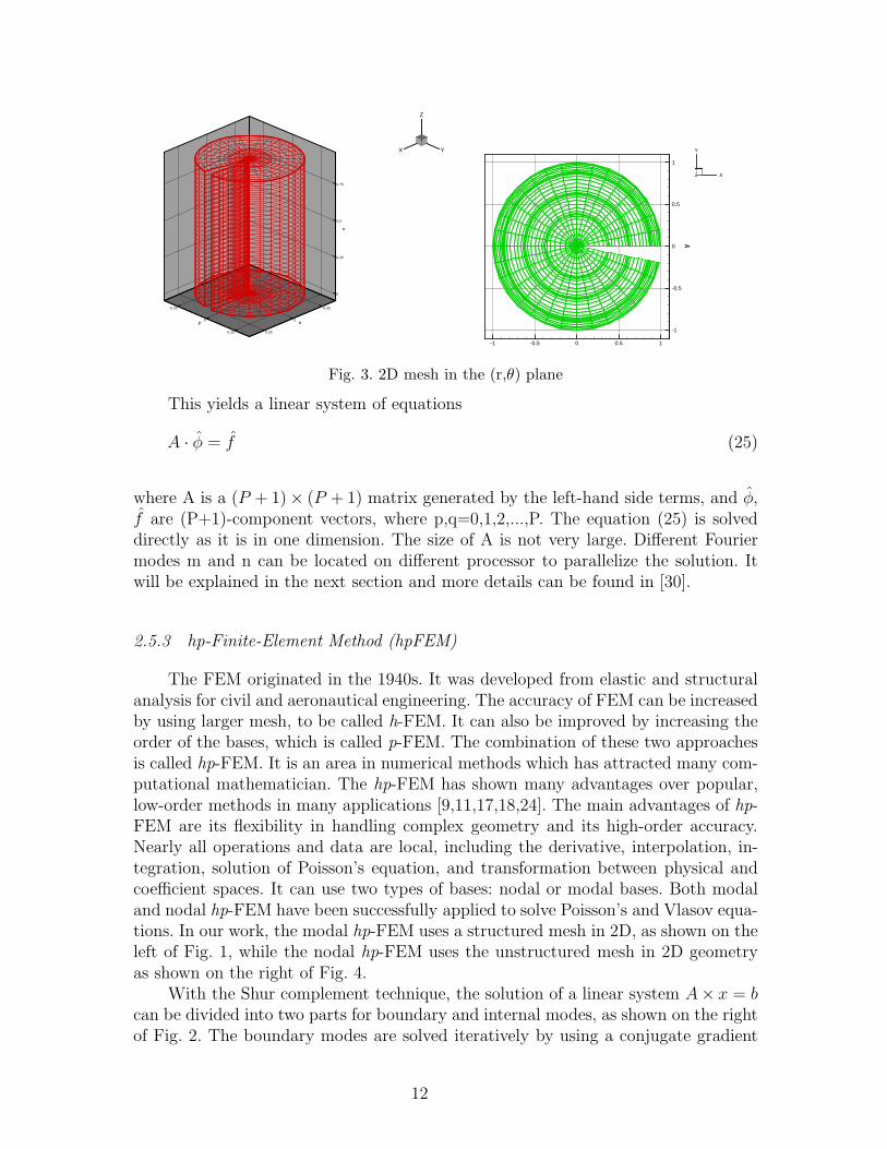
where φ is the electrostatic potential, ρ is the charge density, and ε0 is the permittivityof vacuum. The 3D mesh is shown on the left of Fig. 3. The 2D mesh in the (r,θ)plane is shown on the right of Fig. 3. We use Gauss-Radau-Legendre quadraturepoints [18] in the first element close to the center to avoid the 1/r singularity. Inthis case, there are four unequal elements in the radial direction. Each element hasnine points, and each pair of adjacent elements share the boundary points. Periodicboundary condition (B.C.) have been applied in the longitudinal and circumferentialdirections, and a natural B.C. has been applied in the center of the cylinder. ADirichlet zero B.C. has been applied at r = r0, where r0 is the radius of the cylinder.

By transfroming from the (r, θ, z) space to the (r, m, n) space through FourierTransform, we obtain

1

r

∂

∂r(r

∂φ

∂r) − m2

r2φ − n2φ = − ρ

ε0

(24)

11

0

0.25

0.5

0.75

z

-0.25

0

0.25

x

-0.25

0

0.25

y

X Y

Z

-1

-0.5

0

0.5

1

y

-1 -0.5 0 0.5 1

X

Y

Z

Fig. 3. 2D mesh in the (r,θ) plane

This yields a linear system of equations

A · φ = f (25)

where A is a (P + 1)× (P + 1) matrix generated by the left-hand side terms, and φ,f are (P+1)-component vectors, where p,q=0,1,2,...,P. The equation (25) is solveddirectly as it is in one dimension. The size of A is not very large. Different Fouriermodes m and n can be located on different processor to parallelize the solution. Itwill be explained in the next section and more details can be found in [30].

2.5.3 hp-Finite-Element Method (hpFEM)

The FEM originated in the 1940s. It was developed from elastic and structuralanalysis for civil and aeronautical engineering. The accuracy of FEM can be increasedby using larger mesh, to be called h-FEM. It can also be improved by increasing theorder of the bases, which is called p-FEM. The combination of these two approachesis called hp-FEM. It is an area in numerical methods which has attracted many com-putational mathematician. The hp-FEM has shown many advantages over popular,low-order methods in many applications [9,11,17,18,24]. The main advantages of hp-FEM are its flexibility in handling complex geometry and its high-order accuracy.Nearly all operations and data are local, including the derivative, interpolation, in-tegration, solution of Poisson’s equation, and transformation between physical andcoefficient spaces. It can use two types of bases: nodal or modal bases. Both modaland nodal hp-FEM have been successfully applied to solve Poisson’s and Vlasov equa-tions. In our work, the modal hp-FEM uses a structured mesh in 2D, as shown on theleft of Fig. 1, while the nodal hp-FEM uses the unstructured mesh in 2D geometryas shown on the right of Fig. 4.

With the Shur complement technique, the solution of a linear system A× x = bcan be divided into two parts for boundary and internal modes, as shown on the rightof Fig. 2. The boundary modes are solved iteratively by using a conjugate gradient

12

Y

X

Z

-0.1 0 0.1x

-0.1

-0.05

0

0.05

0.1

y

Fig. 4. Modal bases (left) and mesh (right) on triangle.

method. The internal modes in each element can then be solved directly. The discretesystem for the Poisson equation can be written as follows:

Abb Cbi

CTbi Aii

ub

ui

=

fb

fi

, where b and i correspond to boundary and interior variables and ub and ui can besolved separately by the following equations:

(Abb − CbiA−1

ii CTbi)ub = fb − CbiA

−1

ii fi (26)

ui = A−1

ii (fi − CTbiub) (27)

More details can be found in [9,18].

Since the Vlasov solver on an unstructured grid is built on the DG framework, Itis better to solve the Poisson’s equation with the DG method too. The method beenused in DG framework is called interior penalty (IP) method [2,10,26], more detailscan be found in [32].

3 Parallel Methods

In order to use petascale supercomputers, the numerical methods explainedabove must be parallelized. As in the preceding section, the parallel methods willbe explained in three subsections. Since the Poisson solver is of special importancein BDS and its parallelization is the most challenging, it is explained separately.

13

3.1 Parallel Method for PIC Software

A BDS has two components: particle tracking and space charge (SC) calculation.For the PIC solver in PTRACK, we use domain decomposition only for the SCcomponent of the calculation, which is the parallel Poisson solver explained below.The parallel algorithm for the PTRACK is shown in Fig. 5. At the beginning of thecalculation, the internally generated or read-in initial particle distribution is equallydistributed among all the processors. That is, each processor has only part of thetotal particles. But each processor has information about the full external fields forthe beamline or accelerator element being simulated. The SC grid is also defined onall the processors. Before every tracking step the internal SC fields of the beam mustbe computed and combined with the external fields. The first step in the calculationof SC fields is the particle charge deposition on the nodes of the SC grid. This is donelocally; that is, each processor deposits the charges of particles that are located on it.At the end of this step, every processor will have a partial SC distribution includingonly the charge of its particles. To calculate the SC distribution of the whole beam, wesum the partial SC distributions on the SC grid using the “MPI Allreduce” routineof the MPI Library [23], To use domain decompositions of the Poisson solver shownin Fig. 7, we subdivide the full SC grid into smaller-scale SC grids using 1D, 2D,and 3D space decompositions. Each processor will have a local SC grid containingonly part of the SC data. FSM has been used for all these three decompositions.Since the FFT is a global transformation, in order to perform FFT in one directionall data in that direction should be collected on one processor. Then after FFT,they will be distributed back to their original processors. After solving the Poissonequation, we have the solution in the form of potential data distributed on the localgrids of each processor. In order to have all potential on each processor, a secondglobal communication using “MPI Allreduce” will bring the potential data from thelocal grids to the global grid to be ready for the tracking part of the calculation.The complete procedure is summarized in Fig. 5. The domain decomposition methodhas been used for the parallelization of other Poisson solvers, such as the Fourierhp-Finite Element Method. More details can be found in [28].

3.2 Parallel Method for direct Vlasov Solvers

For 1P1V, which is equivalent to a 2D simulation, 1D domain decomposition inboth physical x and velocity vx space has been adopted. Two MPI communicators,comx and comv, have been generated for operations in different spaces. For 2P2Vsimulation using the structured grid, the parallel model performs 2D domain decom-positions in both physical (x, y) and velocity (vx, vy) planes; therefore, completely 4Ddomain decomposition has been used, as shown on the left of the Fig. 6. This makes iteasy to use a large number of processors and is particularly helpful for direct solutionof the Vlasov equation. Three splitting substeps are associated with different com-

14

Partial SC on each processor

Charge deposition on SC grid

Next Tracking step

Previous Tracking step

Sum−up partial SC’s for full SC

Parallel Poisson Solver

Solution (Potential) on local SC grids

Full Potential data on each processor Collect local Potential data to global grid

Main Sequence (Serial) Parallel sequence

Distribute full SC data to N local SC grids

Fig. 5. Parallel algorithm of PTRACK

x’

y’

o’

x

y

o

4D Phase Space

Fig. 6. Structured (left) and unstructured (right) grid in 2D plane

municators. This makes it possible to solve the Vlasov in high dimensions. In thesesimulations, two more communicators, comxy and comvxvy, have been generatedfor operations in different planes. The communicator comxy contains all processorswith the same (vx, vy) location, and comvxvy contains all processors with the same(x, y) location. These two communicators are used for computing the beam statistics.When using the unstructured grid, only two communicators can be created, whichare comxy and comvxvy, because it is impossible to distinguish x from y on the (x,y) plane and vx from vy on the (vx, vy) plane. Details in each case can be found in[31,32].

15

xo

y

zxo

y

z

Fig. 7. Parallel models for the Fourier spectral method

3.3 Parallel Methods for Poisson Solvers

Because of the global nature of Poisson’s equation, involving the whole chargedistribution to calculate an effective self-field created by all the particles in the beam,its parallelization is the most challenging part in developing scalable algorithms forBDS. Especially when the grid is small and a large number of processors is used.In this section, we summarize the parallel algorithms developed with the domaindecomposition method.

3.3.1 Parallel Method for FSM

Since FSM is the most popular method for solving Poisson’s equation, more workhas been devoted to this method. Three domain decomposition methods have beenimplemented, as shown in Fig. 7. With the appropriate model, it is easy to use tens ofthousands of processors with a relatively small grid for the space charge calculation.For example, if the grid used for Poisson’s equation is 323, then the maximum numberof processors that can be used is 32 for the 1D decomposition model, 322 = 1024 forthe 2D decomposition model and 323 = 32, 768 for the 3D decomposition model.If the data is not located in one processor in any direction, a global MPI Alltoallneeds to be called to transfer the data into one processor. Another call is needed totransfer back the data to their original processors. Good scaling has been obtainedwith a relatively small grid for the space charge calculation, see [27–29].

3.3.2 Parallel Method for Fhp-FEM

For the Fhp-FEM in CYLCS, 2D domain decomposition has been developed,as shown in Fig. 8. The model on the right has the benefit of solving the 1D linearsystem A × x = b on each processor, as they are totally decoupled. While the modelon the left has to solve the boundary modes first, then the internal modes in eachelements in the r direction. Since the element number in the r direction is not very

16

Fig. 8. Parallel models for the Fourier hp-finite element method

large, this model is also efficient and it is being used for BDS. It is also possibleto develop 3D domain decomposition, as was done for FSM, which can use a largenumber of processors. Details can be found in [31].

3.3.3 Parallel Method for hp-FEM

Parallel Poisson solvers using hp-FEM are achieved by using the Shur comple-ment technique, shown on the right of Fig. 2. The boundary mode, equation (26), hasbeen solved using an iterative conjugate gradient (CG) method, whereas the internalmode of each element, equation (27), has been solved by the direct method. Themesh should be partitioned appropriately so that all processors have approximatelythe same numbers of elements to ensure load balance. In order to speedup the CGmethod, an efficient preconditioner can be used. For the multigrid technique, boththe coarse and fine meshes use the same mesh partition. This makes it convenientto perform prolongation and restriction operations on each element. A good meshpartition is to minimize the modes located on the interfaces of different processors,as this will reduce the communication cost during global operations. More details canbe found in [32].

4 Comparison and Discussion

In this section we compare the performance of the numerical methods presentedin the paper. The comparison may help to understand these methods in more depth.

4.1 PIC vs. DVM

The common point of PIC and DVM is that they both need to solve the Poisson’sequation during each time step. PIC and DVM have many differences, however. PICuses a Lagrangian approach, while DVM uses an Euler approach. Using Lagrangian

17

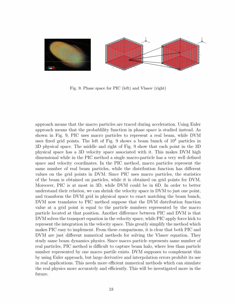
Fig. 9. Phase space for PIC (left) and Vlasov (right)

approach means that the macro particles are traced during acceleration. Using Eulerapproach means that the probablility function in phase space is studied instead. Asshown in Fig. 9, PIC uses macro particles to represent a real beam, while DVMuses fixed grid points. The left of Fig. 9 shows a beam bunch of 108 particles in3D physical space. The middle and right of Fig. 9 show that each point in the 3Dphysical space has a 3D velocity space associated with it. This makes DVM highdimensional while in the PIC method a single macro-particle has a very well definedspace and velocity coordinates. In the PIC method, macro particles represent thesame number of real beam particles, while the distribution function has differentvalues on the grid points in DVM. Since PIC uses macro particles, the statisticsof the beam is obtained on particles, while it is obtained on grid points for DVM.Moreover, PIC is at most in 3D, while DVM could be in 6D. In order to betterunderstand their relation, we can shrink the velocity space in DVM to just one point,and transform the DVM grid in physical space to exact matching the beam bunch,DVM now translates to PIC method suppose that the DVM distribution functionvalue at a grid point is equal to the particle numbers represented by the macroparticle located at that position. Another difference between PIC and DVM is thatDVM solves the transport equation in the velocity space, while PIC apply force kick torepresent the integration in the velocity space. This greatly simplify the method whichmakes PIC easy to implement. From these comparisons, it is clear that both PIC andDVM are just different numerical methods for solving the Vlasov equation. Theystudy same beam dynamics physics. Since macro particle represents same number ofreal particles, PIC method is difficult to capture beam halo, where less than particlenumber represented by one macro partile exists. DVM supposes to complement thisby using Euler approach, but large derivative and interpolation errors prohibit its usein real applications. This needs more efficient numerical methods which can simulatethe real physics more accurately and efficiently. This will be investigated more in thefuture.

18

4.2 SLM vs. DGM

SLM and DGM are two efficient methods for time integration. Both methodshave strong stability. While DGM has stronger stability than the continuous Gar-lekin method (CGM), SLM is supposed to be unconditionally stable. DGM has strictlimitation on the time step size while SLM is less limited. Therefore, with the ap-propriate choice of the time step size, SLM could be more stable than DGM. Since abeam is a concentrated bunch of particles, the distribution function could have sharpstructures; this makes the errors of interpolation and derivation much larger thanin usual plasma simulations. The greatest challenge comes from these large operatorerrors. In practical, SLM is easier to develop than the DGM. For the parallelization,as DG has completely independent bases on each element, the communication is lessexcept for the DG Poisson solver. While the SLM has to redistribute all back tracingpoints on different processors, which makes it more complicated than DG. There isalso a load balancing problem in SLM, since only small portion of the phase spacehas probability function larger than some value. Depending on the mesh partition,usually most back tracing points are located on some processors. This wastes thecomputing time, while DG has more balanced computing load as all processor haveequal mount of work to be done.

4.3 Poisson Solvers

Several numerical methods to solve Poisson’s equation have been presentedbriefly. Among them, FSM is the most popular and efficient one. Since the FastFourier Transform (FFT) algorithm can be used and public FFT libraries are easilyavailable. The drawback of FSM is the global characteristics of Fourier Transforma-tion. This requires the data in one direction must locate on one processor to completethe FFT. The large ratio of communication cost over the FFT cost makes the parallelefficiency low on large number of processors. As the total time is small compared toother time in PIC and direct Vlasov solvers, the overall parallel efficiency still good.This fits in all three parallel methods been developed for FSM, especially the oneusing 3D domain decomposition which can be run efficiently on tens of thousands ofprocessors. Fhp-FEM is designed for CYLCS, which gives a more accurate solutionfor a cylindrical geometry because the B.C. is more precisely defined on a cylinderwall. Since the hp-FEM has been used in the radial direction, this limit the numberof processors that can be used. The number of processors used in Fhp-FEM usuallyis less than that of FSM. High-order accuracy can be achieved by hp-FEM Poissonsolvers when using high-order polynomials. Similar to FSM, there is some inherentrestriction on scalability. Since the modes on interface between elements is solvedglobally through conjugate gradient method, the parallel efficiency usually becomeworse when the number of processors increases. The parallel efficiency usually be-comes better as the polynomial order increases for both CG and DG methods. The

19

convergence of CG usually is better than the DG method. Using an unstructuredgrid makes it easy to handle complex geometries, which also requires more work inthe development. These Poisson solvers are more or less effective in different config-urations and the choice of the appropriate solver should be based on the geometryand boundary conditions.

4.4 Structured vs. Unstructured meshes

Unstructured mesh is more appropriate for complex geometries, and finer meshcan be generated in the central part of the beam. Both structured and unstructuredmeshes can apply CG or DG methods, but of course the unstructured mesh is morecomplicated to develop. One significant difference between structured and unstruc-tured meshes for the 2P2V Vlasov solvers is that we don’t have access to the samestatistical quantities. As explained in the previous section for parallel models forVlasov solvers, using an unstructured mesh it is not possible to seperate the x andy directions. There is no way to find all (x, vx) points for a given (y, vy) point. Sim-ilarly There is no way to find all (y, vy) points for a given (x, vx) point. Therefore,the statistical quantities XX ′

rms and Y Y ′

rms can not be calculated, while the statis-tical quantities Xrms, Yrms, X ′

rms, and Y ′

rms can be obtained on both meshes. Thedefinitions of these statistics can be found in [31].

5 Summary

We presented a summary of efficient numerical and parallel methods used anddeveloped in our research for large scale beam dynamics simulations during the past5 years at ANL. Hope it will be helpful to other researchers in accelerator simula-tions. They have been explained in brief and readers should consult the cited journalarticles for more details. These numerical methods have been discussed in three cat-egories: PIC, DVM, and Poisson solvers. Parallel methods for all of them have alsobeen described in following. These methods are intended to enable the numericalmethods to take advantage of petascale supercomputers. The parallel methods havebeen implemented in software packages and successfully run on tens of thousands ofprocessors of the IBM Blue Gene/P at the Argonne Leadership Computing Facil-ity. The parallel PIC solver, PTRACK, has been used for large-scale beam dynamicoptimization and real accelerator simulations. The parallel DVM solvers have beendeveloped in 1P1V and 2P2V simulations, they have provided much more detail in-formation on the physics, such as halo generation and filamentation in low dimensionand with smooth initial distribution functions. Due to the large derivation and in-terpolation errors, they are difficult being used in real accelerator simulations now.More efficient numerical methods need to be developed to simulate complex beamdynamics more accurately. This will be investigated more in the future. More ever,

20

direct Vlasov solevrs have more potential applications in plasma physics. Necessaryfor the success of PIC and VDM, several numerical methods for solving the Poisson’sequation in different situations have been presented and compared. They are criticalto perform the large scale simulations of BDS. Overall, these numerical and parallelmethods serve as a basis for BDS, and they can be applied to more broad areas inthe future. The numerical methods discussed in this paper are only summary in ourresearch at ANL, there are many other efficient numerical methods which have notbeen included. In the future, more efficient numerical methods will be adopted toimprove current BDS. At the same time, the current ones will be further optimized.

Acknowledgment

This paper is based on research conducted in the Physics and Mathematics andComputer Science Divisions at ANL during the past 5 years. Besides the co-authorslisted, many other people have contributed to the work reported here, and we thankthem for their contributions. We also thank Gail Pieper in MCS at ANL for theproofreading. This work was supported by the U.S. Department of Energy, Office ofNuclear Physics, under Contract No. DE-AC02-06CH11357.

References

[1] T.D. Arber and R.G.L. Vann, A critical comparison of Eulerian-grid-based Valsovsolvers, J. Sci. Comp., 180, 339–357 (2002).

[2] D.N. Arnold, F. Brezzi, B. Cockburn, and L.D. Marini, Unified analysis of discontinuousGalerkin methods for elliptic problems, SIAM J. Numer. Anal., 39, no. 5, 1749–1779(2002).

[3] V.N. Aseev, P.N. Ostroumov, E.S. Lessner, and B. Mustapha, TRACK: The new beamdynamics code. In Proceedings of PAC-05 Conference, Knoxville, Tennessee, May 16–20, 2005.

[4] C. Canuto, M.Y. Hussaini, A. Quarteroni, and T.A. Zang, Spectral Methods in FluidMechanics, Springer-Verlag, New York, 1987.

[5] C.Z. Cheng and G. Knorr, The integration of the Vlasov equation in configurationspace, J. Sci. Comp., 22, 330–351 1976.

[6] B. Cockburn, Discontinuous Galerkin methods for convection-dominated problems. InHigh-Order Methods for Computational Physics, edited by T. Barth and H. Deconink,Lecture Notes in Computational Science and Engineering, Vol. 9, Springer Verlag,Berlin, 1999, pp. 69–224.

21

[7] B. Cockburn, G. Karniadakis, and C.W. Shu, eds., The development of discontinuousGalerkin methods. In Discontinuous Galerkin Methods. Theory, Computation andApplications, Lecture Notes in Computational Science and Engineering, Vol. 11,Springer Verlag, Berlin, 2000, pp. 3–50.

[8] B. Cockburn and C.W. Shu, Runge-Kutta discontinuous Galerkin methods forconvection-dominated problems, J. Sci. Comp., 16, 173–261 (2001).

[9] M.O. Deville, P.F. Fischer, and E.H. Mund, High-Order Methods for IncompressibleFluid Flow, Cambridge University Press, Cambridge, 2002.

[10] J. Douglas, Jr., and T. Dupont, Interior Penalty Procedures for Elliptic and ParabolicGalerkin Methods, Lecture Notes in Physics, Vol. 58, Springer Verlag, Berlin, 1976.

[11] M. Dubiner, Spectral methods on triangles and other domains, J. Sci. Comp., 6, 345–390, (1991).

[12] F. Filbet and E. Sonnendrucker, Modeling and numerical simulation of space chargedominated beams in the paraxial approximation, Mathematical Models and Methods inApplied Sciences, 16, no.5, 763–791 (2006).

[13] Paul Fischer, James Lottes, David Pointer, and Andew Siegel, Petascale algorithms forreactor hydrodynamics, Journal of Physics: Conference Proceedings, 125, no. 1, 012976(2008).

[14] D. Gottlieb and S.A. Orszag, Numerical Analysis of Spectral Methods: Theory andApplications, SIAM-CMBS, 1977.

[15] L. Greengard and J. Lee, A direct adaptive Poisson solver of arbitrary order accuracy,J. Comput. Phys., 125, 415–424 (1996).

[16] J.S. Hesthaven and T. Warburton, Nodal high-order methods on unstructured grids, I:Time-domain solution of Maxwell’s equations, J. Comput. Phys., 181, 186–221 (2002).

[17] J.S. Hesthaven and T. Warburton, Nodal Discontinuous Galerkin Methods: Algorithms,Analysis and Applications, Springer, New York, 2008.

[18] G.E. Karniadakis and S.J. Sherwin, Spectral/hp Element Methods for CFD, OxfordUniversity Press, London, 1999.

[19] T. Koornwinder, Two-variable analogues of the classical orthogonal polynomials. InTheory and Applications of Special Functions, edited by M. Ismail and E. Koelink,Academic Press, San Diego, 1975.

[20] A.T. Patera, A spectral element method for fluid dynamics: Laminar flow in a channelexpansion, J. Comput. Phys., 54, 468–488 (1984).

[21] W.H. Reed and T.R. Hill, Triangular mesh methods for the beutron transport equation,Tech. Report LA-UR-73-479, Los Alamos Scientific Laboratory, Los Alamos, NM, 1973.

[22] G. Strang and G.J. Fix, An Analysis of the Finite Element Method, Wellesley-Cambridge Press, Wellesley, 2008.

[23] B. Szabo and I. Babuska, Finite Element Analysis, Wiley, New York, 1991.

22

[24] J. Shen and T. Tang, Spectral and High-Order Methods with Applications, Science Pressof China, 2006.

[25] E. Sonnendrucker, F. Filbet, A. Friedman, E. Oudet, and J.-L. Vay, Vlasov simulationsof beams with a moving grid, Comput. Phys. Comm., 164, 2390–395 (2004).

[26] M.F. Wheeler, An elliptic collocation-finite element method with interior penalties,SIAM J. Numer. Anal., 15, 152–161 (1978).

[27] J. Xu, Benchmarks on Tera-scalable Models for DNS of Channel Turbulent Flow,Parallel Computing. 33/12, 780-794, 2007.

[28] J. Xu, B. Mustapha, V.N. Aseev, and P.N. Ostroumov, Parallelization of a beamdynamics code and first large scale radio frequency quadrupole simulations, PhysicsReview Special Topic–Accelerator and Beams, 10, 014201 (2007).

[29] J. Xu, B. Mustapha, V. N. Aseev, and P.N. Ostroumov, Simulations of high-intensitybeams using BG/P supercomputer at ANL. In Proceedings of HB 2008, Nashville,Tennessee, Aug. 25–29, 2008.

[30] J. Xu and P.N. Ostroumov, Parallel 3D Poisson solver for space charge calculation incylinder coordinate system, Computer Physics Communications, 178, 290–300 (2008).

[31] J. Xu, B. Mustapha, P.N. Ostroumov, and J. Nolen, Solving 2D2V Vlasov equationwith high order spectral element method, Communication in Computational Physics,8, 159–184 (2010).

[32] J. Xu, P.N. Ostroumov, J. Nolen, and K.J. Kim, Scalable direct Vlasov solver withdiscontinuous Galerkin method on unstructured mesh, SIAM Journal on ScientificComputing.

[33] J. Xu , P. N. Ostroumov, B. Mustapha, M. Min and J. Nolen Developing Peta-scalableAlgorithms for Beam Dynamic Simulations, Proceeding of IPAC10, Kyoto, Japan, May23-28, (2010).

23