Efficient estimation for case-cohort studies

By BIN NAN

Department of Biostatistics, University of Michigan, 1420 Washington Heights,

Ann Arbor, Michigan 48109, U.S.A.

bnan@umich.edu

December 2, 2002

Summary

In this paper we consider time-to-event data from case-cohort designs. In view of the fact

that the existing methods are either inefficient or requiring particular censoring assumptions,

we develop a semiparametrically efficient estimator under the usual assumptions for Cox re-

gression models. The estimator is obtained by one iteration of the Newton-Raphson algorithm

that solves the efficient score equations with initial values being obtained from existing meth-

ods, and shown to be consistent, asymptotically efficient and normally distributed. Simulations

show that the proposed estimators perform well in finite samples, and considerably improve the

efficiency of the existing pseudo-likelihood estimators when a correlate of the missing covariate

is available. We focus on the situation where covariates are discrete, and also explore how to

apply the method to models with continuous covariates.

Some key words: Case-cohort design, Cox model, efficient score, integral equation, martingale operators,

mean residual life operators, missing at random, Newton-Raphson algorithm

1

1. Introduction

Case-cohort designs, a type of cost effective biased sampling designs originally proposed by

Prentice (1986) and further studied by Self & Prentice (1988), are widely used in epidemiology

studies with time-to-event data. In a case-cohort design, the complete information is observed

for all failures and a simple random sub-sample of the entire cohort. It is essentially equivalent

to collecting complete information for all failures and a simple random sub-sample of the non-

failures, which can be viewed as an example of two-phase sampling studies. Borgan et al. (2000)

studied the so-called exposure stratified case-cohort designs, where the complete information

is collected for all the failures and a stratified random sub-sample of the non-failures. The

stratification is based on some easily observable covariate, a correlate of the true “exposure”,

which is available for the entire cohort. They showed that the stratified sampling designs can

increase estimating efficiency dramatically using the weighted version of the pseudo-likelihood

estimating methods.

Case-cohort designs are very useful in designing large epidemiological cohort studies for

rare diseases when the information of some covariates is hard or expensive to collect, in which

the information is only collected for a small proportion of the study subjects. It is very

easy to obtain a long list of recent publications using such studies by searching PubMed.

Since the classical case-cohort designs can be viewed as special cases of the exposure stratified

case-cohort designs, we call both of them case-cohort designs throughout in the paper except

where they need to be distinguished. When these designs are conducted using independent and

identically distributed sampling scheme, which is what we assume in this paper, they are within

the framework of two-phase sampling designs. Studies of efficient scores for semiparametric

regression models in two-phase designs can be found in the author’s 2001 dissertation.

2

The existing estimating methods are based on the pseudo-likelihood proposed originally by

Prentice (1986). As being pointed out by Nan et al. (2002), these methods are inefficient and

can lose efficiency dramatically in certain situations. The research on efficient estimators for

Cox regression with missing data starts to appear recently. Chen & Little (1999) and Herring

& Ibrahim (2001) proposed likelihood-based methods via an EM algorithm assuming that (i)

the censoring time distribution does not depend upon the covariates that are only observable

for a sub-sample of the subjects; and (ii) the joint distribution of covariates is known up to

a finite-dimensional parameter. Under these assumptions, the terms that are related to the

censoring distribution are factored out from the full likelihood, and the integration with respect

to the covariates with missing data in the likelihood function is computable. Thus maximizing

the likelihood becomes possible via an EM algorithm approach. But their assumptions are

not often realistic in practice. Our goal is to find efficient estimators without these extra

assumptions.

In Section 2 we review existing estimating methods for case-cohort studies briefly. In

Section 3 we discuss the efficient score functions for case-cohort designs. In Section 4 we

propose the efficient estimators for the case-cohort designs with discrete covariates by solving

the efficient score equations using one step Newton-Raphson approximation. Large sample

properties for the proposed estimators are discussed in Section 5. Simulations are listed in

Section 6, which follows by a brief discussion. Proofs are provided in the Appendix.

2. Existing Estimating Methods

We briefly review current estimating methods for analyzing data from case-cohort studies.

Let T be the failure time and C be the censoring time. Suppose the underlying “full” data con-

sist of n independent and identically distributed copies of (Y, ∆, X, V ), where Y = min{T, C}

3

is the observed time, ∆ = 1(T ≤ C) is the failure indicator, X is the covariate (vector) of

interest, and V is a covariate (vector) that is correlated with X. We assume that given (X,V ),

T and C are independent. We will mainly discuss the situation that V is the surrogate of

X, which means that T is independent of V given X, or equivalently that V is a variable

that is not involved in the Cox model for failure time. There are situations that some other

covariates V ′ should be included in the Cox model and their information is easily collectable

for all subjects. These situations can be converted to the situation with only (X, V ) by making

an identical copy of V ′ and combining each of the two copies of V ′ into X and V , separately.

So it is adequate to discuss the situation with (X, V ) only, where V is not involved in the Cox

model.

In an exposure stratified case-cohort design, we observe (∆, V ) for every subject in the study

cohort, which is the Phase-I of the two-phase sampling study. Then we obtain a sub-sample by

stratified sampling, the Phase-II of the study, based on Phase-I data with sampling probabilities

P (R = 1|Y,∆, X, V ) = P (R = 1|∆, V ) ≡ π(∆, V ) = 1 if ∆ = 1, and 0 < σ ≤ π(∆, V ) ≤ 1 if

∆ = 0. Here R is an indicator with value 1 if subject is in the sub-sample and 0 otherwise. And

we observe (Y, X) for the sub-sample obtained at Phase-II. In a classical case-cohort design, V

is not available or not used. Then the Phase-II sampling probabilities are only dependent on ∆.

We want to estimate the effect of the covariate X on the survival time, the parameter θ, based

upon the Cox proportional hazards assumption, which assumes that the survival probability

conditional on X has the following form

SF (t) ≡ 1− F (t|X = x) = P (T > t|X = x) = exp(− Λ(t)eθ′x

),

where we assume T |X ∼ F (· |X).

These designs can be used both prospectively and retrospectively. Suppose X is some kind

of biology measurement(s) from tissue samples. In a prospective study, we measure V for every

4

subjects at the very beginning, and then select a random sub-sample from the study cohort

with pre-specified probabilities based on V . We follow the entire cohort up to the end of study

and collect the information of X for all the failures and the subjects in the sub-sample. The

measuring of X can be done whenever the tissue is available. In an retrospective study, we

do Phase-II sampling retrospectively with probabilities π(∆, V ) and measure X only for the

selected sub-sample from their frozen tissues, assuming that the measurements of X do not

deteriorate.

Suppose π(∆, V ) is given by the investigators who design the studies, then the above

problems are missing data problems with data missing at random, a terminology of Little &

Rubin (1987), and known missingness probabilities. Currently, most of the estimating methods

for θ are based on modifications of the partial likelihood estimating equations for full data

proposed by Cox (1972, 1975), which is, using integration notation, as following:

n∑

i=1

∫ τ

0

{Xi −

∑nj=1 1(Yj ≥ t)eθ′XjXj∑n

j=1 1(Yj ≥ t)eθ′Xj

}dNi(t) = 0. (1)

Here n is the total number of subjects in the study cohort, τ is the time of the end of study,

and {N(t) : 0 ≤ t ≤ τ} is the failure counting process.

Prentice (1986) proposed pseudo-likelihood estimating equations for the classical case-

cohort studies, where V is not available or not used:

m∑

i=1

∫ τ

0

{Xi −

∑j∈C 1(Yj ≥ t)eθ′XjXj∑

j∈C 1(Yj ≥ t)eθ′Xj

}dNi(t) = 0. (2)

Here m is the total number of subjects with X being measured and C is a simple random sub-

sample of the study cohort, the so-called sub-cohort. Every subjects in the sub-cohort are fully

observed. Since all failures are fully observed, the real difference between (1) and (2) is the

second term inside the integrals. Both of them are consistent estimators of E[X|Y = t,∆ = 1].

The term in (1) is estimated by the full data, and the term in (2) is estimated by a simple

5

random sub-sample of the full data. Large sample properties of the estimators based on (2)

are studied by Self & Prentice (1988).

Exposure stratified case-cohort designs are more general than classical case-cohort designs.

A family of estimating equations for θ in these designs is a weighted version of the pseudo-

likelihood estimating equation (2):

m∑

i=1

∫ τ

0

{Xi −

∑mj=1 1(Yj ≥ t)eθ′XjXjwj∑m

j=1 1(Yj ≥ t)eθ′Xjwj

}dNi(t) = 0 , (3)

where wj are weights for subjects. The most often used weights are the inverse sampling

probabilities. Equation (2) can be modified into (3) by including all fully observed subjects

(subcohort plus all failures) in the second term within the integrals. Many authors have

studied the estimating equation (3) for missing data problems in Cox regression, including

Lin & Ying (1993), Chen & Lo (1999), and Borgan et al. (2000). Though we know that the

partial likelihood estimators based on equation (1) are fully efficient if there is no missing data,

the estimators based on equations (2) or (3) are known not to be efficient for missing data

problems, see e.g. Nan et al. (2002).

Other inefficient estimating methods include imputation of missing covariate values for the

partial likelihood score equation, see e.g. Paik & Tsai (1997); or estimating the partial likeli-

hood function with missing values based on observed data and then maximizing the estimated

partial likelihood, see e.g. Zhou & Pepe (1995).

3. Efficient Score Function

We derive in this section the efficient score of θ under the Cox proportional hazards as-

sumption for case-cohort studies. Define an operator D as

Du(Y, ∆, X, V ) =∫

u(t,X, V ) dM(t),

6

where M(t) is the martingale of failure counting process N(t) with the following form under

the Cox proportional hazards assumption:

M(t) = ∆1(Y ≤ t)−∫

1(Y ≥ s)eθ′X dΛ(s) ,

where Λ(·) is the cumulative baseline hazard.

For case-cohort studies, π(∆, V ) = 1 if ∆ = 1. Following Nan et al. (2002), one can show

that the efficient score function for θ can be written as

l∗θ =R

π(∆, V )Du(Y,∆, X, V )− R− π(∆, V )

π(∆, V )E[Du(Y,∆, X, V )|∆, V ] ; (4)

where the function u(y, x, v) is determined by the following operator equation

u(y, x, v)−{

Ku(y, x, v)− E[Ku(Y, X, V )|Y = y, ∆ = 1]}

= x− E[X|Y = y, ∆ = 1] , (5)

and the operator K is given by

Ku(y, x, v) = E[b(Y, ∆, X, V )|Y > y, X = x, V = v] (6)

with

b(Y, ∆, X, V ) =1− π(∆, V )

π(∆, V )

{Du(Y,∆, X, V )− E[Du(Y, ∆, X, V )|∆, V ]

}.

Since b(Y, 1, X, V ) = 0, by the equation (6) and the definition of R1 operator in Nan et al.

(2002), we have

Ku(y, x, v) =1

1−W (y|x, v)

∫ ∞

yb(t, 0, x, v) dW 0(t|x, v) , (7)

where W (y|x, v) = W 1(y|x, v) + W 0(y|x, v) is the conditional distribution function of Y given

(X, V ) = (x, v), and W 1(y|x, v) and W 0(y|x, v) are the conditional sub-distributions of Y given

(X, V ) = (x, v) corresponding to ∆ = 1 and ∆ = 0, separately.

7

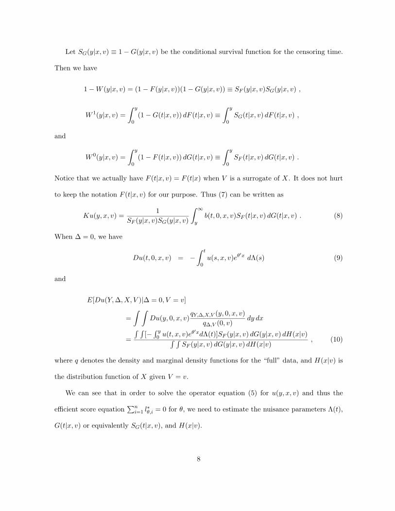
Let SG(y|x, v) ≡ 1−G(y|x, v) be the conditional survival function for the censoring time.

Then we have

1−W (y|x, v) = (1− F (y|x, v))(1−G(y|x, v)) ≡ SF (y|x, v)SG(y|x, v) ,

W 1(y|x, v) =∫ y

0(1−G(t|x, v)) dF (t|x, v) ≡

∫ y

0SG(t|x, v) dF (t|x, v) ,

and

W 0(y|x, v) =∫ y

0(1− F (t|x, v)) dG(t|x, v) ≡

∫ y

0SF (t|x, v) dG(t|x, v) .

Notice that we actually have F (t|x, v) = F (t|x) when V is a surrogate of X. It does not hurt

to keep the notation F (t|x, v) for our purpose. Thus (7) can be written as

Ku(y, x, v) =1

SF (y|x, v)SG(y|x, v)

∫ ∞

yb(t, 0, x, v)SF (t|x, v) dG(t|x, v) . (8)

When ∆ = 0, we have

Du(t, 0, x, v) = −∫ t

0u(s, x, v)eθ′x dΛ(s) (9)

and

E[Du(Y,∆, X, V )|∆ = 0, V = v]

=∫ ∫

Du(y, 0, x, v)qY,∆,X,V (y, 0, x, v)

q∆,V (0, v)dy dx

=

∫ ∫[− ∫ y

0 u(t, x, v)eθ′xdΛ(t)]SF (y|x, v) dG(y|x, v) dH(x|v)∫ ∫SF (y|x, v) dG(y|x, v) dH(x|v)

, (10)

where q denotes the density and marginal density functions for the “full” data, and H(x|v) is

the distribution function of X given V = v.

We can see that in order to solve the operator equation (5) for u(y, x, v) and thus the

efficient score equation∑n

i=1 l∗θ,i = 0 for θ, we need to estimate the nuisance parameters Λ(t),

G(t|x, v) or equivalently SG(t|x, v), and H(x|v).

8

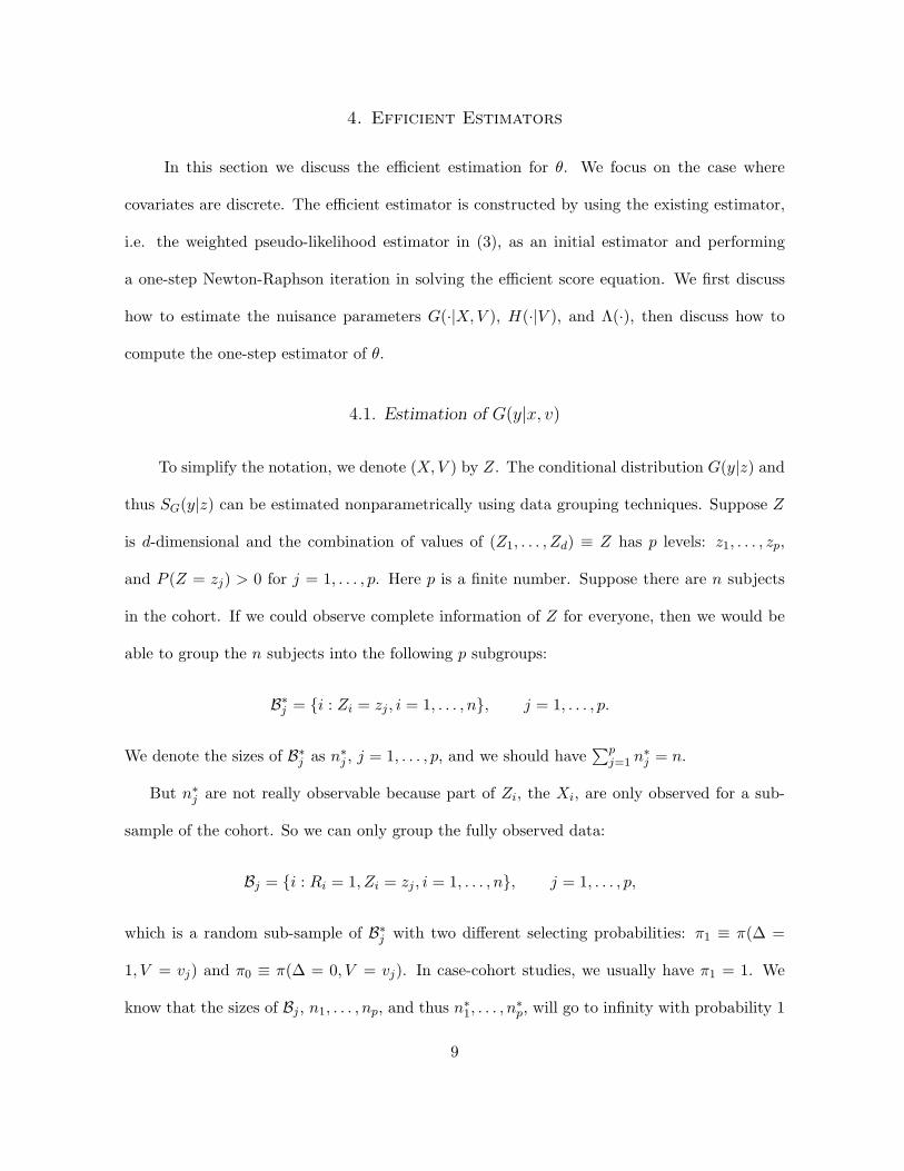
4. Efficient Estimators

In this section we discuss the efficient estimation for θ. We focus on the case where

covariates are discrete. The efficient estimator is constructed by using the existing estimator,

i.e. the weighted pseudo-likelihood estimator in (3), as an initial estimator and performing

a one-step Newton-Raphson iteration in solving the efficient score equation. We first discuss

how to estimate the nuisance parameters G(·|X, V ), H(·|V ), and Λ(·), then discuss how to

compute the one-step estimator of θ.

4.1. Estimation of G(y|x, v)

To simplify the notation, we denote (X, V ) by Z. The conditional distribution G(y|z) and

thus SG(y|z) can be estimated nonparametrically using data grouping techniques. Suppose Z

is d-dimensional and the combination of values of (Z1, . . . , Zd) ≡ Z has p levels: z1, . . . , zp,

and P (Z = zj) > 0 for j = 1, . . . , p. Here p is a finite number. Suppose there are n subjects

in the cohort. If we could observe complete information of Z for everyone, then we would be

able to group the n subjects into the following p subgroups:

B∗j = {i : Zi = zj , i = 1, . . . , n}, j = 1, . . . , p.

We denote the sizes of B∗j as n∗j , j = 1, . . . , p, and we should have∑p

j=1 n∗j = n.

But n∗j are not really observable because part of Zi, the Xi, are only observed for a sub-

sample of the cohort. So we can only group the fully observed data:

Bj = {i : Ri = 1, Zi = zj , i = 1, . . . , n}, j = 1, . . . , p,

which is a random sub-sample of B∗j with two different selecting probabilities: π1 ≡ π(∆ =

1, V = vj) and π0 ≡ π(∆ = 0, V = vj). In case-cohort studies, we usually have π1 = 1. We

know that the sizes of Bj , n1, . . . , np, and thus n∗1, . . . , n∗p, will go to infinity with probability 1

9

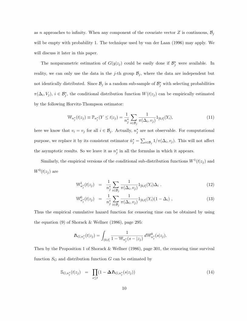
as n approaches to infinity. When any component of the covariate vector Z is continuous, Bj

will be empty with probability 1. The technique used by van der Laan (1996) may apply. We

will discuss it later in this paper.

The nonparametric estimation of G(y|zj) could be easily done if B∗j were available. In

reality, we can only use the data in the j-th group Bj , where the data are independent but

not identically distributed. Since Bj is a random sub-sample of B∗j with selecting probabilities

π(∆i, Vj), i ∈ B∗j , the conditional distribution function W (t|zj) can be empirically estimated

by the following Horvitz-Thompson estimator:

Wn∗j (t|zj) ≡ Pn∗j (Y ≤ t|zj) =1n∗j

∑

i∈Bj

1π(∆i, vj)

1[0,t](Yi), (11)

here we know that vi = vj for all i ∈ Bj . Actually, n∗j are not observable. For computational

purpose, we replace it by its consistent estimator n∗j =∑

i∈Bj1/π(∆i, vj). This will not affect

the asymptotic results. So we leave it as n∗j in all the formulas in which it appears.

Similarly, the empirical versions of the conditional sub-distribution functions W 1(t|zj) and

W 0(t|zj) are

W1n∗j

(t|zj) =1n∗j

∑

i∈Bj

1π(∆i, vj)

1[0,t](Yi)∆i . (12)

W0n∗j

(t|zj) =1n∗j

∑

i∈Bj

1π(∆i, vj)

1[0,t](Yi)(1−∆i) , (13)

Thus the empirical cumulative hazard function for censoring time can be obtained by using

the equation (9) of Shorack & Wellner (1986), page 295:

IΛG,n∗j (t|zj) =∫

(0,t]

11−Wn∗j (s− |zj)

dW0n∗j

(s|zj).

Then by the Proposition 1 of Shorack & Wellner (1986), page 301, the censoring time survival

function SG and distribution function G can be estimated by

SG,n∗j (t|zj) =∏

s≤t

(1−∆IΛG,n∗j (s|zj)) (14)

10

=∏

Ynj :i≤t,i∈Bj

{1− 1/π(∆(i), vj)

n∗j −∑i−1

k=1 1/π(∆(k), vj)

}1−∆(i)

,

and

Gn∗j (t|zj) = 1− SG,n∗j (t|zj)

= 1−∏

Ynj :i≤t,i∈Bj

{1− 1/π(∆(i), vj)

n∗j −∑i−1

k=1 1/π(∆(k), vj)

}1−∆(i)

, (15)

where ∆IΛG,n∗j (s|zj) is the jump of IΛG,n∗j (t|zj) at time t = s, Ynj :i are the ordered times,

and ∆(i) and π(∆(i), vj) are the corresponding values of censoring indicators and sampling

probabilities.

Another way to think of estimating ΛG(t|zj) is to solve the following inverse-probability-

weighted estimating equation for all subjects in Bj :

∑

i∈Bj

1π(∆i, vj)

{(1−∆i)1[0,t](Yi)−

∫

[0,t]1[Yi≥s] dΛG(s|zj)

}= 0 .

By discretizing ΛG(t|zj) we will obtain the same ∆IΛG,n∗j (Yn∗j :i) as in (14).

4.2. Estimation of H(x|v)

In order to estimate the conditional distribution function H(x|v), we group data based

on the values of V similarly to that in the previous subsection:

C∗j = {i : Vi = vj , i = 1, . . . , n}, and Cj = {i : Ri = 1, Vi = vj , i = 1, . . . , n}.

Let the size of C∗j be n∗j and the size of Cj be nj . Similar to the estimation of W (t|zj), a

Horvitz-Thompson type of estimator for H(x|V = vj) would be

Hn∗j (x|vj) =1n∗j

∑

i∈Ci

1π(∆i, vj)

1[Xi≤x] . (16)

Here n∗j is not observable, but can be estimated by∑

i∈Cj1/π(∆i, vj).

11

4.3. Estimation of Λ(t)

For a given θ, the cumulative baseline hazard Λ(·) can be estimated by a generalization

of the Breslow estimator where full data are available:

Λn,θ(t) =n∑

i=1

1(Yi ≤ t)λi,θ, with λi,θ =∆i∑n

j=1 1(Yj ≥ Yi)Rj

πjeθ′Xj

, (17)

which is n1/2-consistent, see e.g. Borgan et al. (1995). Thus SF (y|x, v) = SF (y|x) = e−Λ(y)eθ′x

and dF (y|x, v) = dF (y|x) = eθ′x−Λ(y)eθ′xdΛ(y) can be estimated by replacing Λ(·) by Λn,θ.

4.4. Estimation of θ

An efficient estimator for θ can be obtained by replacing all the parameters by their

preliminary estimators in equation (5) to solve for u(y, x, v), and then plugging those estimated

parameters and the solution of equation (5) into the efficient score function (4) to solve the

equation∑n

i=1 l∗θ,i = 0 for θ. We mainly discuss the one-step estimator here, since an initial

n1/2-consistent estimator for θ, θn, can be easily obtained from existing methods, such as

solving the equation (3). The comparison of the converged solution from multiple iterations

and its one iteration approximation, the one-step estimator, is illustrated by simulations.

Now we show how to handle the pieces of the integral equation (5). For any initial θ, an

estimator Kθ(u) for the operator K(u) in (8) can be obtained by plugging the estimators of

all other parameters into (9), (10), and then (8). Then we can estimate

E[K(u)(Y, X, V )|Y = y, ∆ = 1] =E[1(Y ≥ y)eθ′XK(u)(Y, X, V )]

E[1(Y ≥ y)eθ′X ](18)

by estimating both the numerator and denominator using weighted averages. Thus the above

conditional expectation of operator K can be estimated by

E[K(u)(Y, X, V )|Y = y, ∆ = 1] =n∑

i=1

1(Yi ≥ y) Riπ(∆i,Vi)

eθ′Xi

∑nk=1 1(Yk ≥ y) Rk

π(∆k,Vk)eθ′Xk

Kθ(u)(Yi, Xi, Vi) . (19)

12

Since the nonparametric estimators SG(y|x, v) and H(x|v) only jump on observed data points,

both Kθ(u) and E[K(u)(Y, X, V )|Y, ∆ = 1] will be linear combinations of the values of u(y, x, v)

on the grid of {observed Yi’s}⊗{observed (Xi, Vi)’s}. Assume that the number of distinct

values of observed Yi’s is nY . Then the integral equation (5) automatically becomes a linear

system as follows:

u(Yi, Xj , Vj)− Kθ(u)(Yi, Xj , Vj) +n∑

k=1

1(Yk ≥ Yi) Rkπ(∆k,Vk)e

θ′Xk

∑ns=1 1(Ys ≥ Yi) Rs

π(∆s,Vs)eθ′Xs

Kθ(u)(Yk, Xk, Vk)

= Xj −n∑

k=1

1(Yk ≥ Yi) Rkπ(∆k,Vk)e

θ′Xk

∑ns=1 1(Ys ≥ Yi) Rs

π(∆s,Vs)eθ′Xs

Xk, (20)

where i = 1, . . . , nY , j = 1, . . . , p, and p is the number of distinct values of (Xi, Vi)’s as before.

If Y is continuous, the number of distinct values of Y will be the number of fully observed

records with probability 1.

The above linear system has a unique solution, which will be discussed in the next section.

Solving for nY × p unknown values of u(y, x, v), we obtain the solution uθ(Yi, Xj , Vj). Thus

the efficient score in (4) can be estimated by replacing u by uθ and all the parameters by their

preliminary estimators:

l∗n,θ(Ui) =Ri

π(∆i, Vi)

{∆iuθ(Yi, Xi, Vi)−

n∑

k=1

1(Yk ≤ Yi)uθ(Yk, Xi, Vi)eθ′Xi λk,θ

}

− Ri − π(∆i, Vi)π(∆i, Vi)

E[D(uθ(Y, ∆, X, V )|∆ = ∆i, V = Vi] . (21)

Here Ui ≡ (Ri, RiYi, ∆i, RiXi, Vi) denotes the i-th record in the cohort. If ∆i = 1, we do not

need to worry about the conditional expectation in (21), because Ri = π(∆i, Vi) = 1. We only

need to calculate the estimators of (10) for all the records with ∆ = 0.

Let I(θ) = E[l∗θ l∗Tθ ] be the information for θ. Then we have I(θ) = −E[∂l∗θ/∂θ], since

0 =∫

l∗θdPθ,η and thus

0 =∫

(∂l∗θ/∂θ)dPθ,η +∫

l∗θ lTθ dPθ,η = E

[ ∂

∂θl∗θ

]+ E[l∗θ l

Tθ ] = E

[ ∂

∂θl∗θ

]+ E[l∗θ l

∗Tθ ]. (22)

13

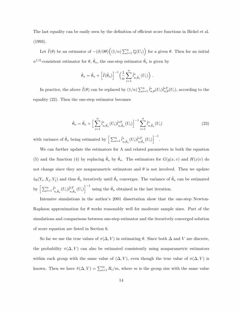
The last equality can be easily seen by the definition of efficient score functions in Bickel et al.

(1993).

Let I(θ) be an estimator of −(∂/∂θ)((1/n)

∑ni=1 l∗θ(Ui)

)for a given θ. Then for an initial

n1/2-consistent estimator for θ, θn, the one-step estimator θn is given by

θn = θn +[I(θn)

]−1( 1n

n∑

i=1

l∗n,θn

(Ui))

.

In practice, the above I(θ) can be replaced by (1/n)∑n

i=1 l∗n,θ(Ui)l∗Tn,θ(Ui), according to the

equality (22). Then the one-step estimator becomes

θn = θn +[ n∑

i=1

l∗n,θn

(Ui)l∗Tn,θn(Ui)

]−1n∑

i=1

l∗n,θn

(Ui) (23)

with variance of θn being estimated by[ ∑n

i=1 l∗n,θn

(Ui)l∗Tn,θn(Ui)

]−1.

We can further update the estimators for Λ and related parameters in both the equation

(5) and the function (4) by replacing θn by θn. The estimators for G(y|x, v) and H(x|v) do

not change since they are nonparametric estimators and θ is not involved. Then we update

uθ(Yi, Xj , Vj) and thus θn iteratively until θn converges. The variance of θn can be estimated

by[ ∑n

i=1 l∗n,θn

(Ui)l∗Tn,θn(Ui)

]−1using the θn obtained in the last iteration.

Intensive simulations in the author’s 2001 dissertation show that the one-step Newton-

Raphson approximation for θ works reasonably well for moderate sample sizes. Part of the

simulations and comparisons between one-step estimator and the iteratively converged solution

of score equation are listed in Section 6.

So far we use the true values of π(∆, V ) in estimating θ. Since both ∆ and V are discrete,

the probability π(∆, V ) can also be estimated consistently using nonparametric estimators

within each group with the same value of (∆, V ), even though the true value of π(∆, V ) is

known. Then we have π(∆, V ) =∑m

i=1 Ri/m, where m is the group size with the same value

14

of (∆, V ), and the sum of the second term of (21) will be zero. Thus the calculation of the

sum of the score functions in (21) can be simplified to

n∑

i=1

l∗n,θ(Ui) =n∑

i=1

Ri

π(∆i, Vi)

{∆iuθ(Yi, Xi, Vi)−

n∑

k=1

1(Yk ≤ Yi)uθ(Yk, Xi, Vi)eθ′Xi λk,θ

}.

This calculation should be asymptotically equivalent to the previous calculation with true

π(∆, V ). The simulations conducted in Section 6 use the true π(∆, V ).

5. Large Sample Properties

In this section, we will discuss the solutions of the integral equation (5) and the asymptotic

properties of the estimators of all the parameter under the following assumptions:

Assumption 1: The covariate Z ≡ (X, V ) is bounded, and the conditional distribution of

T given Z possesses a continuous Lebesgue density.

Assumption 2: The study stops at a finite time t = τ > 0 such that infz∈ZP (C ≥ τ |Z =

z) = infz∈ZP (C = τ |Z = z) = σ1 > 0 and infz∈ZP (T > τ |Z = z) = σ2 ∈ (0, 1).

The linear operator equation (5) can be rewritten as an integral equation with following

form:

u(y, x, v)−∫

M1(y, y′, x, v)u(y′, x, v) dy′

−∫

M2(y, x, y′, x′, v)u(y′, x′, v) dµ(y′, x′)

−∫

M3(y, x, v, y′, x′, v′)u(y′, x′, v′) dν(y′, x′, v′) = f(y, x, v).

In general, this is not a standard Fredholm integral equation of the second kind, though

similar. The properties of this kind of integral equation remain unknown. But when the

covariates Z = (X,V ) are discrete with p distinct levels, the above integral equation reduces

to a system of p Fredholm integral equations of the second kind.

15

For simplicity, we look at a simple example with a single binary covariate Z = X ∈ {x1, x2}.

Let u(y, x1) = u1(y) and u(y, x2) = u2(y). Then the equation (5) can be written as the

following system of linear integral equations with two unknown functions u1(y) and u2(y):

{u1 −A11u1 −A12u2 = f1,

u2 −A21u1 −A22u2 = f2.(24)

Under Assumptions 1 and 2, the integral operators Aij , i, j = 1, 2 are Hilbert-Schmidt and

thus compact, see e.g. Reed & Simon (1972). The argument about the compactness of these

integral operators can be found in the author’s 2001 dissertation and the lengthy details shall

not be repeated in this paper.

Using the idea of Pogorzelski (1966), pages 181-182, the above system of integral equations

(24) can be reduced to one Fredholm equation. Consequently, the theory of a system of

Fredholm integral equations can be reduced to the theory of one Fredholm equation without

any new difficulties. Thus the compactness of the integral operators in (24) guarantees that

the Riesz theory applies to the reduced one Fredholm equation of the second kind, see e.g.

Kress (1999), Chapter 3. This also holds for cases with p > 2.

Lemma 5.1. Suppose all the preliminary estimators for the parameters θ, Λ, G(y|x, v),

and H(x|v) are n1/2-consistent, and the terms in equation (5) are continuously differentiable

with respect to these parameters, then the solution of equation (20) is also n1/2-consistent to

the solution of equation (5).

Proof. This is a direct consequence of Theorem 10.1 in Kress (1999), page 164. 2

Lemma 5.2. (i) Suppose that the random covariate vector Z is discrete with finite number

of levels p, and suppose that Assumptions 1 and 2 hold. Then ‖Gn∗j ( · |zj) − G( · |zj)‖∞ → 0

almost surely for j = 1, . . . , p as n →∞. Furthermore, n1/2(Gn∗j ( · |zj)−G( · |zj)), j = 1, . . . , p,

converge weakly to zero-mean Gaussian processes as n → ∞. Here ‖ · ‖∞ is the supremum

norm.

16

(ii) If V is discrete with finite number of levels pv, then ‖Hn∗j ( · |vj)−H( · |vj)‖∞ → 0 almost

surely for j = 1, . . . , pv as n → ∞. Furthermore, n1/2(Hn∗j ( · |vj) − H( · |vj)), j = 1, . . . , pv,

converge weakly to zero-mean Gaussian processes as n →∞.

The proof of Lemma 5.2 is deferred to the Appendix. The following theorem gives us the

desirable asymptotic properties of the one-step estimator for θ, and the proof is also deferred

to the Appendix.

Theorem 5.3. Suppose that the following conditions are satisfied:

1. l∗θ and l∗n,θ are continuously differentiable in a neighborhood Θ of θ0;

2. supθ∈Θ‖l∗n,θ − l∗θ‖ = op(n−1/2);

3. I(θ) is nonsingular and continuous at θ0;

4. supθ∈Θ‖I(θ)− I(θ)‖ → 0 in probability;

5. n1/2(θn − θ0) = Op(1).

Then for the one-step estimator θn in (23), we have n1/2(θn − θ0) → N(0, I(θ0)−1) in

distribution.

In Theorem 5.3, it is easily seen from (4) and (21) that Condition 1 holds for the Cox

regression models in case-cohort studies. Condition 2 holds since Λn,θ, ΛG, H, and uθ are

n1/2-consistent, and the random vector (Y,∆, X, V ) is bounded under Assumptions 1 and 2.

Condition 3 is a usual assumption. Condition 4 is related to Condition 2. Finally, Condition

5 is guaranteed from previous studies, see e. g. Borgan et al. (2000).

6. Simulation Studies

In the simulation studies, we consider the situation in which covariates X and V are binary,

{0, 1}, and failure time is exponentially distributed with constant failure rate λ. We investigate

two types of censoring distributions: C ≡ 1 and C ∼ Uniform. For the point mass censoring

17

time situation, we have the advantage of being able to compare the finite sample variances of

the one-step estimators to the theoretical information bounds that have been developed by the

author, see e.g. the author’s 2001 dissertation or Nan et al. (2002). We compare bias, variance,

etc., of the efficient estimator to the inverse-probability-weighted pseudo-likelihood estimator

as well as the partial likelihood estimator for the full data in several different situations, i.e.

different values for the parameters in the joint distribution. We also compare the performance

between the one-step estimator and the iteratively converged solution of the efficient score

equations.

When the censoring time C is 1, we always observe Y = 1 for censored subjects in the

sample. So dG(y|z) = dG(y|z) = 1 if y = 1 and 0 elsewhere. The survival time is exponentially

distributed with failure rate λeθx, where λ is determined to obtain 10% number of failures in

the cohort prior time t = 1, i.e. P (∆ = 1) = 0.1. When θ = 0, λ = 0.105; when θ = log(2)

and P (X = 1) ≡ hX(1) = 0.5, λ = 0.071.

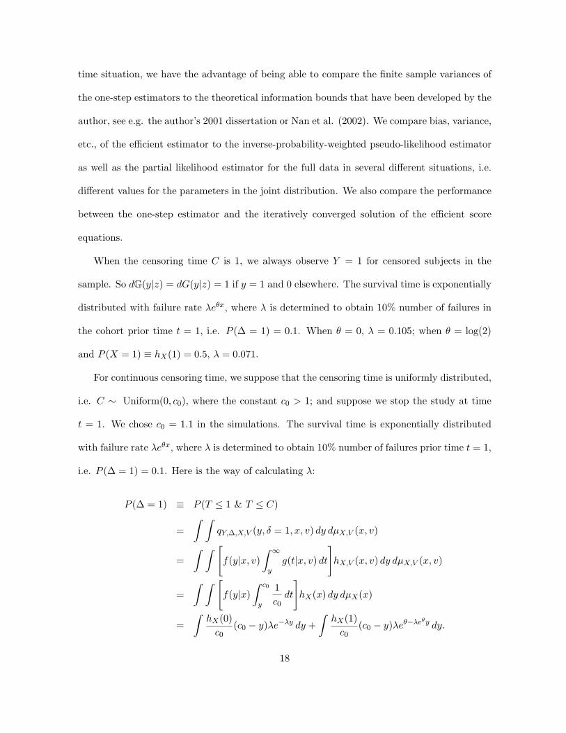
For continuous censoring time, we suppose that the censoring time is uniformly distributed,

i.e. C ∼ Uniform(0, c0), where the constant c0 > 1; and suppose we stop the study at time

t = 1. We chose c0 = 1.1 in the simulations. The survival time is exponentially distributed

with failure rate λeθx, where λ is determined to obtain 10% number of failures prior time t = 1,

i.e. P (∆ = 1) = 0.1. Here is the way of calculating λ:

P (∆ = 1) ≡ P (T ≤ 1 & T ≤ C)

=∫ ∫

qY,∆,X,V (y, δ = 1, x, v) dy dµX,V (x, v)

=∫ ∫ [

f(y|x, v)∫ ∞

yg(t|x, v) dt

]hX,V (x, v) dy dµX,V (x, v)

=∫ ∫ [

f(y|x)∫ c0

y

1c0

dt

]hX(x) dy dµX(x)

=∫

hX(0)c0

(c0 − y)λe−λy dy +∫

hX(1)c0

(c0 − y)λeθ−λeθy dy.

18

Then λ can be solved numerically. When θ = 0, λ = 0.197; When θ = log(2) and hX(1) = 0.5,

λ = 0.132.

The Simulations have been programmed in Splus. Although it is poor in its memory

management and slow for loops, Splus has several appealing features: good random number

generators; internal functions for survival analysis; and a fast program for solving linear sys-

tems. The last one is the most tempting feature for solving our problems and it could save a

lot of programming time. The program is actually run in R instead of Splus, which improves

the simulation speed.

The relationship between X and V can be described by the sensitivity 1 − α and the

specificity 1 − β of V as a rough measurement, a correlate, of X. We consider two levels of

θ: 0 and log(2), and two levels of (α, β): (0.5, 0.5) and (0.3, 0.3). The selection probabilities

π(∆, Vj), j = 1, 2, are determined to have expected one to one case-control matching and equal

size of the two groups of non-failures with V = 0 and V = 1, repectively. The failure probability

prior to time t = 1 is always 0.1. The simulation results with 1000 replications are listed in

Table 1 and Table 2 for point mass censoring and continuous censoring, respectively. Each of

the two tables actually has four simulations. We can see that the one-step estimator and its

variance estimator work reasonably well in these simulations. The estimated information is

very close to the theoretical calculation when C = 1, which can be seen in Table 1. When V

is not correlated with X, the one-step estimator dose not improve the efficiency dramatically

over the pseudo-likelihood estimator. This is because of the low failure rate as being pointed

out by Nan et al. (2002). When V does supply information about X, i.e. the case that

(α, β) = (0.3, 0.3), one-step estimator is obviously superior to the pseudo-likelihood estimator.

The simulations have verified the theoretical arguments in Nan et al. (2002) for the point mass

censoring cases.

19

The comparisons between the one-step estimator and the iteratively converged solution of

the efficient score equation under different situations are listed in Table 3. When the cohort

size is 1000 and the censoring time is uniformly distributed, the converged solution is less

stable than the one-step estimator, i.e., it has larger sample variance (results not shown here).

When we increase the cohort size to 1500, we see that the one-step estimator and the converged

solution work equally well. This phenomenon implies that the one-step estimator has better

performance for small sample size when censoring time is continuous.

7. Discussion

The one-step estimation works well for the case-cohort studies with discrete covariates.

When some covariates are continuous, the efficient estimation becomes more challenging. There

are at least two issues need to be solved: (i) The existence and uniqueness of the solution for

the integral equation (5), or equivalently the integral equation with general form in Section 5,

when some covariates are continuous; (ii) Estimation of the conditional distribution functions

G(· |Z) and H(· |V ). We discuss these problems briefly in this section.

If some components of the covariate vector Z are continuous, we can discretize the function

u(y, z) on a fine grid of the support region of Z. Then for the discretized function u(y, z), the

integral equation (5) reduces to a system of Fredholm integral equations of the second kind.

The number of unknown functions in the system is the number of points on the fine grid of

the support region of Z. By the same argument in Section 5 for the situation of discrete

covariates, the system of integral equations for the discretized function u(y, z) can also reduce

to one Fredholm equation of the second kind. Hence the Riesz theory will apply. We may

expect that the discretized u(y, z) approaches u(y, z) as the grid becomes finer. But we will

face the computational challenge of solving huge linear systems. A natural grid for discretizing

20

u(y, z) is the one that is based on the observed data points.

When covariates are continuous, we may either use smoothing methods to estimate H(· |V )

nonparametrically, or model it parametrically. The conditional distribution function for cen-

soring time, G(· |Z), can be estimated nonparametrically via the data grouping technique used

by van der Laan (1996). A semiparametric method that assumes proportional hazards for cen-

soring time can also be considered to estimate G(· |Z). When nonparametric methods are used

to estimate H(· |V ) or G(· |Z), more study needs to be done on how their convergence rates

affect the asymptotic properties of θn. The work of van der Vaart (2000) should be helpful

in dealing with this problem. According to van der Vaart (2000), if the estimators for all the

nuisance parameters converge no slower than n1/4, then the one-step estimator θn based on

efficient score may still be efficient and asymptotically normal. On the other hand, we may

always obtain a valid estimator if we estimate the nuisance parameters parametrically because

the sampling probabilities π(∆, V ) are known for case-cohort studies, and the expectation of

the score function (4) is zero no matter what u would be. But we may lose efficiency if the

parametric models are not correctly specified.

Numerical calculation is also challenging. A more efficient and generic program needs to

be developed in order to analyze arbitrary data sets.

Acknowledgements

The author would like to thank Jon Wellner for his kind help in this research.

Appendix

Proofs of theoretical results

21

Proof of Lemma 5.2. (i) We can rewrite (11) as

Wn∗j (t|zj) ≡ Pn∗j (Y ≤ t|zj)

=1n∗j

n∑

i=1

1(Zi = zj)Ri

π(∆i, vj)1[0,t](Yi)

=n

n∗j· 1n

n∑

i=1

1(Zi = zj)Ri

π(∆i, vj)1[0,t](Yi)

≡ n

n∗jWn,j(t). (25)

By the strong law of large numbers we have

n∗jn

=1n

n∑

i=1

1(Zi = zj) → E[1(Z = zj)] = P (Z = zj) > 0

almost surely, and

Wn,j(t) → E

[R1(Z = zj)

π(∆, vj)1[0,t](Y )

], almost surely

= E

{E

[R1(Z = zj)

π(∆, vj)1[0,t](Y )

∣∣∣Y,∆, Z

]}

= E

{1(Z = zj)π(∆, vj)

1[0,t](Y )E[R|Y,∆, Z]

}

= E

{1(Z = zj)1[0,t](Y )

}

= P (Y ≤ t, Z = zj).

Thus from (25),

Wn∗j (t|zj) → P (Y ≤ t, Z = zj)P (Z = zj)

= W (t|zj) almost surely for all t ∈ [0, τ ].

Please notice that the n∗j in the estimatorsWn∗j (t|zj),W0n∗j

(t|zj), andW1n∗j

(t|zj) is not observable

and can be replaced by its estimator n∗j =∑

i∈B∗j Ri/π(∆i, vj) =∑

i∈Bj1/π(∆i, vj), since

n∗j/n → P (Z = zj) almost surely by the strong law of large numbers.

The following proof is the same as the proof of Theorem 19.1 in van der Vaart (1998), page

266. For a fixed ε > 0, there exists a partition −∞ = t0 < t1 < . . . < tk = ∞ such that

22

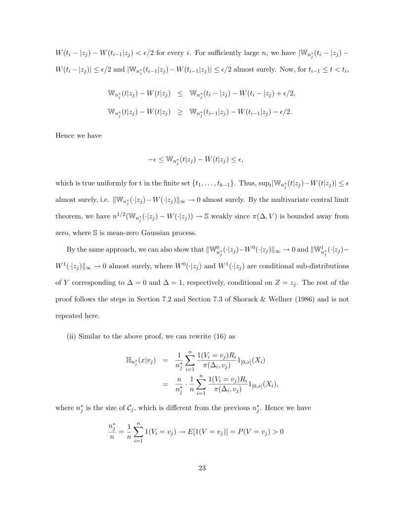
W (ti − |zj) −W (ti−1|zj) < ε/2 for every i. For sufficiently large n, we have |Wn∗j (ti − |zj) −

W (ti−|zj)| ≤ ε/2 and |Wn∗j (ti−1|zj)−W (ti−1|zj)| ≤ ε/2 almost surely. Now, for ti−1 ≤ t < ti,

Wn∗j (t|zj)−W (t|zj) ≤ Wn∗j (ti − |zj)−W (ti − |zj) + ε/2,

Wn∗j (t|zj)−W (t|zj) ≥ Wn∗j (ti−1|zj)−W (ti−1|zj)− ε/2.

Hence we have

−ε ≤Wn∗j (t|zj)−W (t|zj) ≤ ε,

which is true uniformly for t in the finite set {t1, . . . , tk−1}. Thus, supt|Wn∗j (t|zj)−W (t|zj)| ≤ ε

almost surely, i.e. ‖Wn∗j (·|zj)−W (·|zj)‖∞ → 0 almost surely. By the multivariate central limit

theorem, we have n1/2(Wn∗j (·|zj)−W (·|zj)) → S weakly since π(∆, V ) is bounded away from

zero, where S is mean-zero Gaussian process.

By the same approach, we can also show that ‖W0n∗j

(·|zj)−W 0(·|zj)‖∞ → 0 and ‖W1n∗j

(·|zj)−

W 1(·|zj)‖∞ → 0 almost surely, where W 0(·|zj) and W 1(·|zj) are conditional sub-distributions

of Y corresponding to ∆ = 0 and ∆ = 1, respectively, conditional on Z = zj . The rest of the

proof follows the steps in Section 7.2 and Section 7.3 of Shorack & Wellner (1986) and is not

repeated here.

(ii) Similar to the above proof, we can rewrite (16) as

Hn∗j (x|vj) =1n∗j

n∑

i=1

1(Vi = vj)Ri

π(∆i, vj)1[0,x](Xi)

=n

n∗j· 1n

n∑

i=1

1(Vi = vj)Ri

π(∆i, vj)1[0,x](Xi),

where n∗j is the size of Cj , which is different from the previous n∗j . Hence we have

n∗jn

=1n

n∑

i=1

1(Vi = vj) → E[1(V = vj)] = P (V = vj) > 0

23

almost surely, and

1n

n∑

i=1

1(Vi = vj)Ri

π(∆i, vj)1[0,x](Xi) → E

[1(V = vj)R

π(∆, vj)1[0,x](X)

]= P (X ≤ x, V = vj)

almost surely. Thus, Hn∗j (x|vj) → P (X ≤ x|vj) ≡ H(x|vj) almost surely for all x ∈ X .

By using exactly the same method as in the proof of (i), we have ‖Hn∗j (·|vj)−H(·|vj)‖∞ → 0

almost surely. By the multivariate central limit theorem, we have n1/2(Hn∗j (·|vj)−H(·|vj)) → S

weakly since π(∆, V ) is bounded away from zero. 2

Proof of Theorem 5.3. The proof is similar to that in Newey & McFadden (1994). For the

one-step estimator θn in (23), expanding∑n

i=1 l∗n,θn

around θ0 gives

n1/2(θn − θ0) = n1/2(θn − θ0)− n1/2 [I(θn)]−1( 1

n

n∑

i=1

l∗n,θ0(Ui)

)

− [I(θn)]−1[I(θn)]n1/2(θn − θ0)

=(1− [I(θn)]−1[I(θn)]

)n1/2(θn − θ0)− [I(θn)]−1

(n−1/2

n∑

i=1

l∗n,θ0(Ui)

), (26)

where θn is a midpoint of θ0 and θn. By Conditions 3, 4, and 5 we have

‖I(θn)− I(θ0)‖ ≤ ‖I(θn)− I(θn)‖+ ‖I(θn)− I(θ0)‖ → 0

in probability. Hence I(θn)−1 → I(θ0)−1 in probability, and similarly, I(θn) → I(θ0) in

probability. Then using Condition 2, from the above equation (26) we have

n1/2(θn − θ0) = op(1)Op(1)− (I(θ0)−1 + op(1))(n−1/2

n∑

i=1

l∗θ0(Ui) + op(1)

)→ N(0, I(θ0)−1)

in distribution. 2

References

Bickel, P. J., Klaassen, C. A. J., Ritov, Y., & Wellner, J. A. (1993). Efficient and Adaptive

Estimation for Semiparametric Models. Johns Hopkins University Press, Baltimore.

24

Borgan, O., Goldstein, L., & Langholz, B. (1995). Methods for the analysis of sampled

cohort data in the Cox proportional hazards model. Ann. Statist. 23, 1749-1778.

Borgan, O., Langholz, B., Samuelsen, S. O., Goldstein, L., & Pogoda, J. (2000). Exposure

stratified case-cohort designs. Lifetime Data Analysis 6, 39-58.

Chen, H. Y. & Little, R. J. (1999). Proportional Hazards Regression with Missing Covari-

ates. Journal of the American Statistical Association 94, 896-908.

Chen, K. & Lo, S. (1999). Case-cohort and case-control analysis with Cox’s model.

Biometrika 86, 755-764.

Cox, D. R. (1972). Regression models and life tables (with discussion). Journal of the Royal

Statistical Society. B 34, 187-220.

Cox, D. R. (1975). Partial likelihood. Biometrika 62, 269-276.

Herring, A. H. & Ibrahim, J. G. (2001). Likelihood-based methods for missing covariates

in the Cox proportional hazards model. Journal of the American Statistical Association

96, 292-302.

Horvitz, D. G. & Thompson, D. J. (1952). A generalization of sampling without replacement

from a finite universe. Journal of the American Statistical Association 47, 663-685.

Kress, R. (1999). Linear Integral Equations, Second Edition. Springer-Verlag, New York.

Lin, D. Y. & Ying, Z. (1993) Cox regression with incomplete covariate measurements.

Journal of the American Statistical Association 88, 1341-1349.

Little, R. J. A. & Rubin, D. (1987). Statistical Analysis with Missing Data. John Wiley,

New York.

Nan, B., Emond, M., & Wellner, J. A. (2002). Information bounds for Cox regression models

with missing data. Submitted to Ann. Statist.

25

Newey, W. K. & McFadden, D. (1994). Large sample estimation and hypothesis testing.

Handbook of Econometrics, Volum 4. Edited by R. F. Engle and D. L. McFadden. Elsevier

Science B. V., 2113-2245.

Paik, M. C. & Tsai, W-Y (1997). On using the Cox proportional hazards model with missing

covariates. Biometrika 84, 579-593.

Pogorzelski, W. (1966). Integral Equations and Their Applications, Volume 1. PWN-Polish

Scientific Publishers.

Prentice, R. L. (1986). A case-cohort design for epidemiologic cohort studies and disease

prevention trials. Biometrika 73, 1-11.

Reed, M. & Simon B. (1972). Methods of Modern Mathematical Physics I: Functional Anal-

ysis. Academic Press, Inc., New York.

Self, S. G. & Prentice, R. L. (1988). Asymptotic distribution theory and efficiency results

for case-cohort studies. Annals of Statistics 16, 64-81.

Shorack, G. R. & Wellner, J. A. (1986). Empirical Processes with Applications to Statistics.

Wiley, New York.

van der Laan, M. J. (1996). Efficient estimation in the bivariate censoring model and

repairing NPMLE. Annals of Statistics 24, 596-627.

van der Vaart, A. W. (1998). Asymptotic Statistics. Cambridge University Press, Cam-

bridge.

van der Vaart, A. W. (2000). Semiparametric Statistics. Lectures on Probability Theory,

Ecole d’Ete de Probabilites de St. Flour 1999, P. Bernard, Ed. Springer, Berlin; to appear.

Zhou, H. & Pepe, M. S. (1995). Auxiliary covariate data in failure time regression.

Biometrika 82, 139-149.

26

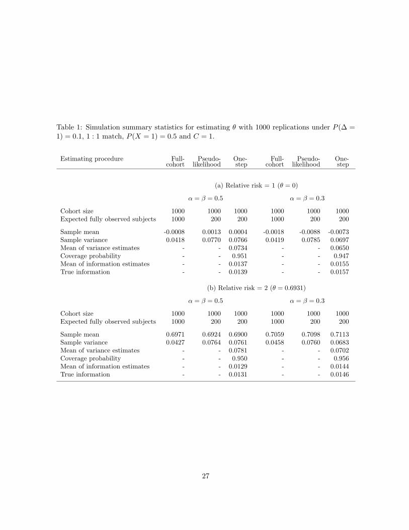
Table 1: Simulation summary statistics for estimating θ with 1000 replications under P (∆ =1) = 0.1, 1 : 1 match, P (X = 1) = 0.5 and C = 1.

Estimating procedure Full- Pseudo- One- Full- Pseudo- One-cohort likelihood step cohort likelihood step

(a) Relative risk = 1 (θ = 0)

α = β = 0.5 α = β = 0.3

Cohort size 1000 1000 1000 1000 1000 1000Expected fully observed subjects 1000 200 200 1000 200 200

Sample mean -0.0008 0.0013 0.0004 -0.0018 -0.0088 -0.0073Sample variance 0.0418 0.0770 0.0766 0.0419 0.0785 0.0697Mean of variance estimates - - 0.0734 - - 0.0650Coverage probability - - 0.951 - - 0.947Mean of information estimates - - 0.0137 - - 0.0155True information - - 0.0139 - - 0.0157

(b) Relative risk = 2 (θ = 0.6931)

α = β = 0.5 α = β = 0.3

Cohort size 1000 1000 1000 1000 1000 1000Expected fully observed subjects 1000 200 200 1000 200 200

Sample mean 0.6971 0.6924 0.6900 0.7059 0.7098 0.7113Sample variance 0.0427 0.0764 0.0761 0.0458 0.0760 0.0683Mean of variance estimates - - 0.0781 - - 0.0702Coverage probability - - 0.950 - - 0.956Mean of information estimates - - 0.0129 - - 0.0144True information - - 0.0131 - - 0.0146

27

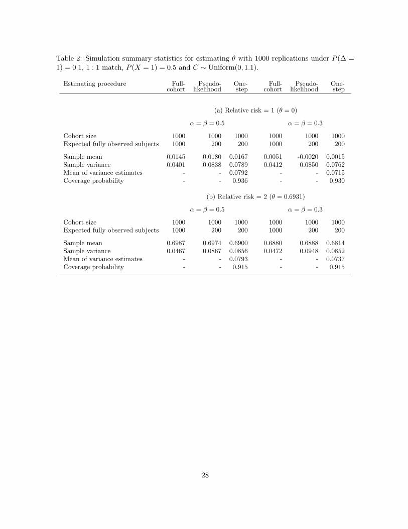
Table 2: Simulation summary statistics for estimating θ with 1000 replications under P (∆ =1) = 0.1, 1 : 1 match, P (X = 1) = 0.5 and C ∼ Uniform(0, 1.1).

Estimating procedure Full- Pseudo- One- Full- Pseudo- One-cohort likelihood step cohort likelihood step

(a) Relative risk = 1 (θ = 0)

α = β = 0.5 α = β = 0.3

Cohort size 1000 1000 1000 1000 1000 1000Expected fully observed subjects 1000 200 200 1000 200 200

Sample mean 0.0145 0.0180 0.0167 0.0051 -0.0020 0.0015Sample variance 0.0401 0.0838 0.0789 0.0412 0.0850 0.0762Mean of variance estimates - - 0.0792 - - 0.0715Coverage probability - - 0.936 - - 0.930

(b) Relative risk = 2 (θ = 0.6931)

α = β = 0.5 α = β = 0.3

Cohort size 1000 1000 1000 1000 1000 1000Expected fully observed subjects 1000 200 200 1000 200 200

Sample mean 0.6987 0.6974 0.6900 0.6880 0.6888 0.6814Sample variance 0.0467 0.0867 0.0856 0.0472 0.0948 0.0852Mean of variance estimates - - 0.0793 - - 0.0737Coverage probability - - 0.915 - - 0.915

28

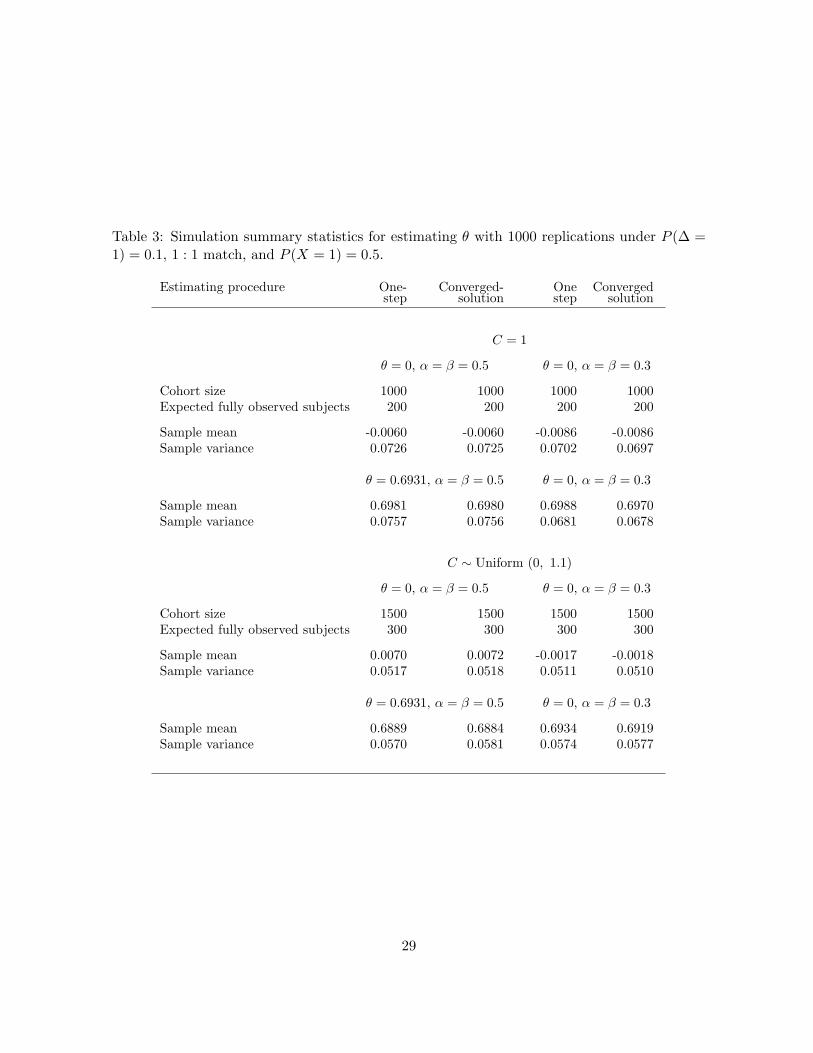
Table 3: Simulation summary statistics for estimating θ with 1000 replications under P (∆ =1) = 0.1, 1 : 1 match, and P (X = 1) = 0.5.

Estimating procedure One- Converged- One Convergedstep solution step solution

C = 1

θ = 0, α = β = 0.5 θ = 0, α = β = 0.3

Cohort size 1000 1000 1000 1000Expected fully observed subjects 200 200 200 200

Sample mean -0.0060 -0.0060 -0.0086 -0.0086Sample variance 0.0726 0.0725 0.0702 0.0697

θ = 0.6931, α = β = 0.5 θ = 0, α = β = 0.3

Sample mean 0.6981 0.6980 0.6988 0.6970Sample variance 0.0757 0.0756 0.0681 0.0678

C ∼ Uniform (0, 1.1)

θ = 0, α = β = 0.5 θ = 0, α = β = 0.3

Cohort size 1500 1500 1500 1500Expected fully observed subjects 300 300 300 300

Sample mean 0.0070 0.0072 -0.0017 -0.0018Sample variance 0.0517 0.0518 0.0511 0.0510

θ = 0.6931, α = β = 0.5 θ = 0, α = β = 0.3

Sample mean 0.6889 0.6884 0.6934 0.6919Sample variance 0.0570 0.0581 0.0574 0.0577

29