Eﬃcient drawing of RNA secondary structurejgaa.info/accepted/2006/Auber+2006.10.2.pdf · Eﬃcient drawing of RNA secondary structure David Auber Maylis Delest ... Therefore the

Journal of Graph Algorithms and Applicationshttp://jgaa.info/ vol. 10, no. 2, pp. 329–351 (2006)

Efficient drawing of RNA secondary structure

David Auber Maylis Delest

Jean-Philippe Domenger Serge Dulucq

LaBRI - Universite Bordeaux 1www.labri.fr

[email protected] [email protected] [email protected] [email protected]

Abstract

In this paper, we propose a new layout algorithm that draws the sec-ondary structure of a Ribonucleic Acid (RNA) automatically accordingto some of the biologists’ aesthetic criteria. Such layout insures that twoequivalent structures (or sub-structures) are drawn in a same and planarway. In order to allow a visual comparison of two RNAs, we use an heuris-tic that places the biggest similar part of the two structures in the sameposition and orientation.

Article Type Communicated by Submitted Revised

Regular paper M. T. Goodrich March 2005 June 2006

Research supported in part by ACI Masse de donnees, Navgraph project.

D. Auber et al., RNA secondary structure, JGAA, 10(2) 329–351 (2006) 330

1 Introduction

Ribonucleic Acid (RNA) is an important molecule, which performs a wide rangeof functions in biological systems. Some RNA is found in the nucleus (where it issynthesized), and in the cytoplasm, as messenger RNA or mRNA (which carriesthe genetic information out of the nucleus), transfer RNA or tRNA (whichdecodes the information), ribosomal RNA or rRNA (which was found in theribosome of cells). These forms of RNA are involved in the protein synthesis.

RNAs recently became the center of much attention because of its catalyticproperties, leading to an increased interest in obtaining structural information.For example, RNA contains genetic information of viruses such as HIV andtherefore regulates the functions of such viruses.

An RNA is characterized by its base sequence and higher order structuralconstraints. It can be considered at three levels of detail :

• its linear sequence of monomers is the primary structure,

• its secondary structure is a two dimensional drawing that reflects majorlinks acting in the RNA,

• its tertiary structure is the three dimensional view where the positions ofatoms are obtained using crystallographic method.

The RNA tertiary structure is often much more highly conserved than the se-quence during evolution. In addition, secondary and tertiary structural featuresof RNAs are important in the molecular mechanism involving their functions.The biologists assume that, for a given RNA, a common function to severalspecies corresponds to a preserved molecular conformation of their RNA and,thus, to a preserved secondary and tertiary structure.

Thus, knowledge of RNA secondary structure is increasingly becoming im-portant in molecular phylogenetic studies, particularly in assisting accurate se-quence alignment [22] that is detecting similar parts between two linear se-quences. Automatic alignment methods that use only primary sequences maymisalign RNA sequences [17] while alignments that take secondary structureinto consideration can generate improved phylogenetic trees [22].

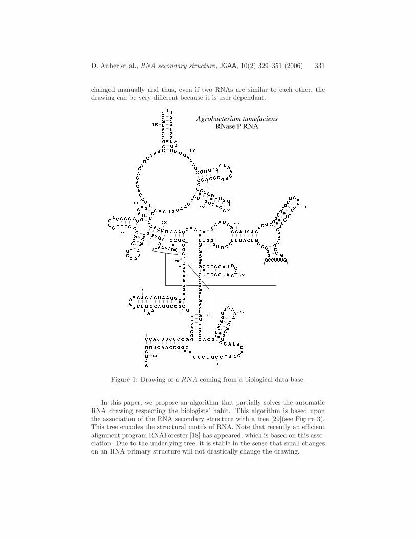
Therefore the ability to draw and visually compare RNA structures is useful.Figure 1 shows an example of hand-drawn RNA secondary structure comingfrom a biologic data base [6]. It refers to structural motifs such as stems,hairpins, bulges, interior loops and multi-branch loops. The goal to achieve isto perform an automatic drawing that respects the biologists’ habit: there areno crossing edges (planar graph), the structural patterns appear clearly.

In the past ten years, many interactive programs allowing interaction withthe RNA drawing were developed. The more recent programs RNAView [32]and RNAViz [26] offer many functionalities such as editing, energy computa-tion, and even three dimensional representation. None of them produces anautomatic planar drawing of an RNA secondary structure that corresponds tothe biologists’ practice. As a consequence, in these programs, the layout is


changed manually and thus, even if two RNAs are similar to each other, thedrawing can be very different because it is user dependant.

Figure 1: Drawing of a RNA coming from a biological data base.

In this paper, we propose an algorithm that partially solves the automaticRNA drawing respecting the biologists’ habit. This algorithm is based uponthe association of the RNA secondary structure with a tree [29](see Figure 3).This tree encodes the structural motifs of RNA. Note that recently an efficientalignment program RNAForester [18] has appeared, which is based on this asso-ciation. Due to the underlying tree, it is stable in the sense that small changeson an RNA primary structure will not drastically change the drawing.


Efficient comparison must allow the user to visually compare two RNA sec-ondary structures. One important requirement to facilitate visual comparisonof structures is to automatically detect parts of the structure that have the sameshape and to place them at the same position and in the same orientation inthe final drawing.This is useful for the user because it will give him reference marks when hewill compare the structures. Thus, in order to present the biologist face to twoRNAs with the same orientation on the screen, we use an heuristic based onquasi-isomorphic subtrees in a tree. This heuristic has been successfully used atthe Infovis’03 contest[3] and is briefly described here. It allows us to place thelargest similar part of two RNAs in a similar position on a portion of the screen(for example at a same relative position from the upper left corner).

In what follows, we first describe the biological background. Then, we de-scribe the drawing algorithm and the heuristic for presenting two RNAs. Finally,we conclude with future work to be done in order to match the requirements ofbiologists.

2 RNA background

An RNA molecule is a linear polymer in which the monomers - (ribo)nucleotides- are linked together by means of phosphodiester bridges, or bonds. Each nu-cleotide contains a base: the four different bases are Adenine (A), Cytosine (C),Guanine (G) and Uracil (U). An RNA sequence R of n nucleotides can be rep-resented as a word of length n on the alphabet {A, C, G, U}: R = r1.r2 . . . rn

where ri is the i-th (ribo)nucleotide belonging to the alphabet. We will refer toi as the ith base of the sequence.Although each RNA molecule has only a single polynucleotide chain, it is nota smooth linear structure. It has extensive regions of base pairs. The com-plementary bases, A-U and G-C form stable base pairs with each other throughthe creation of hydrogen bonds between donor and acceptor sites on the bases.These are called Watson-Crick base pairs whereas the weaker base pair G-U isthe wobble pair. All of these are called canonical base pairs. Other non canonicalbase pairs occur (e.g. A-C and U-U), some of which are stable.

Thus, the secondary structure of an RNA molecule can be viewed as the listof base pairs that occur in its three dimensional structure. In what follows, wewill consider a secondary structure on R as a set P of ordered pairs (i, j), 1 ≤i < j ≤ n, satisfying:

• j − i > 3

• if (i, j) and (k, l) are two base pairs, (assuming without loss of generalitythat i ≤ k ), then either:

– i = k and j = l (they are the same base pair),

– i < j < k < l that is (i, j) precedes (k, l), or

– i < k < l < j that is (i, j) includes (k, l).


Note that the last condition excludes base pairs (i, j) and (k, l) such thati < k < j < l, that is when the two base pairs overlap. A set of base pairs((i+k, j−k))0≤k≤m overlaping a pair (k, l) is called pseudo-knot. Pseudo-knotsare often considered as belonging to tertiary structure. However, pseudo-knotsare real and important structural features.

A hairpin

An interior loop

A bulge

A stem

A multibranch loop

A pseudo-knot

Figure 2: Motifs in a secondary structure.

The RNA secondary structure refers to structural motifs such as stems(S),hairpins(H), bulges (B), interior loops (I) and multi-branch loops(M). RNAstems are self-complementary base-paired regions (A-U, U-A, G-C, C-G), whereashairpins and bulges are regions with unpaired bases; RNA junctions (interiorand multi-branch loops) are the place where two or more stems meet, and theycontain unmatched bases. The overall molecular architecture of the secondary


structure is mainly stabilized by the canonical base pairs A-U, G-C, and G-U. SeeFigure 2.

Following [21], a consequence is that an RNA secondary structure withoutpseudo-knots can be represented as an ordered tree in which each node is labeledand the left to right order among the sibling nodes is significant. The labels ofthe nodes can represent:

• either structural motifs,

• or nucleotides A, C, G, U, Watson-Crick pairs, wobble pairs, . . .

Represented below are (see Figure 3):

1. on the left, an RNA secondary structure, the vertices represent the nu-cleotides,

2. in the center, a relatively rough tree representation of this structure wherethe labels refer to its structural motifs,

3. on the right, a coding of the same structure, the tree with appropriatelabeling of the nodes that makes it possible to come back to the secondarystructure [29, 27].

H

H

H

S

S

S

S S

S

B

I

M

Figure 3: A secondary structure and its tree representations.

Note that this tree representation can be rough (case 2) or refined (case 3).Since the RNA secondary structure appears as a tree-like structure, there

exist works comparing them using tree comparison. Many measures have beenproposed for the similarity of two trees, e.g. tree edit distance, constrained editdistance and alignment of trees [9, 10, 21, 23, 34].

Other related measures can be found in [20, 24, 30]. Alignment of trees is astraightforward extension of sequence alignment that was proved to be differentfrom tree edit distance [21].


An important requirement in a drawing process is to use the knowledgeof users in order to have no conflict with existing representation of the datain the mind of the users. In this particular case, biologists have a long habitof a standard representation of such structures. The drawing of the secondarystructure must be planar, the loops (bulges, hairpins, interior and multi-branch)in the structure should be drawn on circles, and the stems should be drawn on astraight line. Furthermore, the edge length should be constant. Figure 1 showsa hand drawing of a secondary structure made by a biologist. These criteria areequivalent to minimizing three well-known graph drawing criteria which are: theangular resolution, the standard deviation of the edge length, and the numberof crossings. For more information about graph drawing aesthetic criteria onecan refer to [8]. Classical planar drawing algorithms such as the one proposedin [16] do not correspond to the intuitive representation of biologists.

CCAGUUGGCCGGG

CA

GC

CGC

GC

CU

UA

CC

AAUGU

CGAA

AG A

CG

GU

AAG

GUG

AGGAAA

GUCC

G G GC UC

CAC

GGAA

AU

A C GG

UG

CCGGAUAA

CG U C C G G C

GGGGGCGA C

C C C AGGG

AAAGUGCCACAGA

GA

GCAAACC

GC

CA

UG

CCU

U GC

AU

GG

UAAG

GGUG

AA A

GGGU

GG

GGU

AA

G AGC

CCACCGCGCCGCUGG

UG A

CAGUGGUGG C A

AG

GUA

AA

CC

CC

AC

CG

GG

AG

CA

A GA C C G

AA

U A G GG A U G A C A

CG

G GG

CG

GG

CGA A

AGC

CU

GU

UC

AC AGC C G

GU U

UC

CGG

GCCCG

UCAUCCGG

GUGG

GUUGC G AGAGG

C G G C A U G CA

AAUGCCGUCCC

AG

AU

GA

AU

GGCUGCCAC G U

UC

CG

GG U

CA

AACC

GG

GG

CCAUACAGAACC

CG

GC

UU

ACA

GGCCAACUGGC

GAA

Figure 4: Drawing the Agrobacterium tumefaciens with Vienna RNA software.


Other representations can be found in RNA visualization programs [26, 32],however, even if these representations are closer to the biologists’ requirements,some important criteria such as the size of the drawing and the number ofcrossings are not properly taken into account. Figure 4 shows the result of thelayout proposed by one of the latest program, the Vienna package. On thisdrawing, one can see that there are crossings and that loops are not alwaysdrawn on a circle. Thus RNAViz has some tools allowing the user to edit thedrawing.

3 Drawing RNA secondary structure

In order to highlight our algorithm, we have labelled by X, Y and Z thethree main multibranch loops on the RNA hand-drawing (see Figure 5). Asdescribed in section 2, secondary structure of RNA is a chain of nucleotides n1,n2, · · · , nk−1, nk where all ni, ni+1 are linked together and where several linkscan exist between ni, nj with j 6= i+1. Figure 6 shows a sequence of nucleotidesand links. We call Plink (primary structure) the links belonging to the sequence(horizontal links), Slink (secondary structure) the links that form stems andTlink (tertiary structure) the links that create crossings. In Figure 6, the set ofPlinks are the horizontal edges, Slink = 2, 3, 5, 6 and Tlink = 1, 4. If one looksto the structure of RNAs, one can see that the set of nucleotides lie on theouter face of the graph. Thus, the union of Plink and Slink is an outer-planarbiconnected graph. Outer-planar graphs are planar graphs where all verticeslies on a same face (here the external one). One of the nice properties of sucha graph is that one can extract a tree as shown in paragraph 2. Thus, aftertransforming the graph in an outer planar graph (building of the Tlink set) ouralgorithm uses that property in order to reduce the problem of RNA drawingto a problem of tree drawing with a specific set of aesthetic criteria. In whatfollows, we detail the steps of the algorithm.

3.1 Outer-planarization

In the first step, we remove the edges (Tlink) in order to get an outer-planargraph. This can be done using the biologic data basis which point out pseudo-knots or using RNAView. But, knowing that the Plink set forms a Hamiltonianpath in the graph, we can deduce that this path must be the outer-face of theouter-planar graph. Thus, the problem is transformed to the problem of findinga minimum set of edges that enables us to draw the graph without crossing.In Figure 6 one can see the drawing of a graph on one page (that is each edgeis drawn up the sequence). Finding this minimum set consists of building aconflict graph. In this graph a node represents an edge and an edge representsa conflict in the one page drawing. We say that an edge e1 is in conflict withanother edge e2 if and only if e1 intersects e2 in the one page drawing.

If the conflict graph is bipartite, one can compute Tlink easily. Let S1 andS2 be the sets of vertices such that for all vertices u ∈ S1, there exists a vertex


X

Y

Z

Figure 5: The three main multibranch loops.

v ∈ S2 such that u crosses v. We obtain Tlink by choosing the smallest set. Ifthe conflict graph is not bipartite the problem of finding a maximum inducedbipartite subgraph is NP-complete. In order to solve this problem one can usethe heuristic proposed in [2].

Figure 6 shows a conflict graph. From this graph, we remove the edges 1 and4 (Tlink = {1, 4}). One can see in Figure 7 that if the user wants to visualizepseudo-knots (Tlink), these edges can be placed using the third dimension afterthe execution of the drawing algorithm.

After removing the Tlink edges one can compute the tree representationshown on the right of the figure 3. In what follows, we explain how to draw thistree in order to obtain a layout that respects biologist aesthetic criteria. During


6

Conflict graph

1

2

34

5A G U C G U C A G U C

541

Drawing on one page

A

23

6

Figure 6: One page drawing and its conflict graph.

Figure 7: Visualization of pseudo-knots.

our experimentation with data coming from biological data base, the conflictgraph was always bipartite and moreover our algorithm agrees in all cases withbiological data basis on the pseudo-knots.

3.2 Tree drawing

The tree drawing algorithm we have designed is recursive. At each step we firstlayout all the sub-trees induced by the children of a node. Then, we place allthese subtrees drawings on a circle. Literature about similar drawing algorithms


can be found in [7, 14]. In our approach, instead of using a circle hull, we use apacking method inspired by Reingold and Tilford [25] for an efficient hierarchicaltree drawing. However, in our case, the packing is more complex because it is acircular drawing and not a hierarchical one. The main problem is to determinea first coarse radius r of the circle on which one places the subtree drawings.In order to compute this radius, we compute the circumference of the circle onwhich the sub-trees are placed. To find the circumference, we first pack thesub-drawing as a hierarchical drawing does. Then, the width of the boundingbox gives this first circumference. This circumference can be used to obtain thedrawing. However a lot of space is lost because changing from a line to a circlegives more space to use (see Figure 8). Figure 9 shows the result of the packingat the root level and the result on the drawing of the RNA of Figure 1.

Space left

Space left

Space left

Figure 8: Lost space in a simple packing.

Figure 9: Simple packing.

To take this free space into account, we then pack the sub-drawing on a circleinstead of a line. This operation can be done using the same method of packingbut with a transformation from Cartesian coordinates to polar coordinates.


At some level, the drawing can be seen as a sequence of trees whose basis ison a line (see Figure 10 left). For each motif, we compute the real occupiedsector in order to deform the motif. Let us consider the two points M(xM , 0)and N(xN , 0) which are on the basis of a motif. Let I(xI , 0) the middle ofthe segment [M,N ]. For each point P (xP , yp) that delimitates the motif, wecompute the transformed point TP (xTP , yTP ) by

xTP = r∗arcsin((xI −x)/(yTP +r))+xI , yTP =√

(xI − xP )2 + (yP + r)2−r.

One can see in Figure 10 right the effect of the transformation. This transfor-mation then allows to compute a new bounding box that gives in turn a newradius rT which is smaller than r. We then pack the transformated motifs andapply this method until a stable circumference is obtained. Figure 11 showsthe packing of the tree and the result on the entire structure. To obtain anefficient solution we have implemented this packing algorithm with a scan linealgorithm which enables us to obtain drawings of the biggest RNA structuresin a few seconds.

8

8

6

6

4

2

40

20 8

8

6

6

4

2

40

20

Figure 10: Polar transformation.

To prevent overlapping in the final drawing one must force sub-trees to bedrawn outside of the circle. This restriction introduces a lot of long edges inthe final drawing but is necessary in order to have a good angular resolutionin the drawing. In Figure 12 one can see this phenomena on two stems. Inorder to obtain a drawing that matches the aesthetic criteria of the biologistone must make a trade-off between these two aesthetic criteria (edge length,angular resolution). We obtain this trade-off by forcing the drawing of the sub-tree to be on a semi circle. This is done by adding in the packing algorithm twosub-trees (or shape) at the left and at the right. This way also take into accountthe particular case of sub-trees composed of one node. In Figure 12 one can seethese two shapes in black at the left and at right of the drawing. Even if thesemi circle seems to be the best solution according to our experimentation one


Figure 11: Polar packing.

can use this as a parameter to choose the trade-off between the edge length andthe angular resolution.

Inserted shapes

Figure 12: (left) Shape insertion, (right) Bad edge length.

3.3 Final drawing

In Figure 13, the tree is displayed in blue and the sequences in red. One can seethat several nodes are shared between the tree and the sequence (green), thusto obtain the final drawing we have to set coordinates for the nodes that formstems (red). Knowing that each of these nodes is associated with a node η ofthe tree (grey box), we can compute the position of these nodes by placing themon a line orthogonal to the line formed by the coordinates of η and father(η).This operation is straightforward using a cross product. The main problem nowis to determine the distance between the node and η. In order to prevent thenodes from overlaping, we set the size of η three times bigger (one node, a spaceand one node) in the tree drawing algorithm. Thus, we are sure that if a node


is at distance 3

2from η, no overlapping will occur. Figure 14 shows the result of

our algorithm on the graph of the Figure 1 and the Figure 15 shows both sideby side. Note that it would be easy now to deforme the circles in order to fitthe hand drawing.

Figure 13: Sets of nodes.

4 RNAs pairwise Placement

In this section, we use a combination of metrics in order to predict commonparts in several RNAs in order to help the user in the alignment process. Wehave shown in section 2 that the secondary structure of an RNA is associatedwith a tree. At the Infovis’03 Conference contest [12] on pairwise comparisonof trees, an assigned task was to find similar subtrees that have moved :

• the subtrees are not in the same place in the hierarchy,

• slight changes occure between the two subtrees

First note that “finding isomorphic subtrees in a tree” or “common subtreesin several trees” are one and the same task. In the last case, one just needs toconstruct a tree with a vertex (its root), which has subtrees that are the treesto be compared. Thus, using the underlying tree of two RNAs, “find similarparts on RNAs” can be turned to “find similar subtrees in a tree”. Works hasalready been done based on vertices degrees by Zemlyachenko [33] and then byDinitz et al. [31]. These algorithms give a partition of subtrees into isomorphismequivalence classes. They are proved to be linear. However, they only detectisomorphism and do not provide a measure of similarity for subtrees. More


Figure 14: Drawing Agrobacterium tumefaciens with our algorithm

recently, Gupta et al. [15] gave a nice algorithm for determining the largest treeembeddable in two trees. It would be usable in our context but the complexityof their algorithm is O(n2) for non parallel computer. In our case, we want afaster algorithm because the RNA placement is computed on data bases (severalthousands of RNAs) and this algorithm must also work on a personal computer.Moreover, we do not want the largest one but mainly the largest similar one,which means that we accept some slight changes. In order to give a response tothe Infovis’03 task, we have designed an heuristic [3] that can suggest by colorsmeaning similar parts in a tree (similar subtrees have same colors). Thus, we areable to use the graph drawing algorithm of section 3 to automatically displaytwo RNAs and (using our heuristic) to color them in order to suggest to the userwhich parts of the RNAs are similar. The last task is to present the final imagesof the two RNAs such that the user can easily identify the common parts. Wedecided to place the center of the biggest (in term of nodes of the underlyingsubtrees) similar parts at the same coordinate. If there are several choices thenwe choose one at random. Thus we apply a rotation to the drawing. Below, webriefly describe the heuristic. Let s be a vertex. We compute the four followingmetrics :

• the degree of the vertex denoted by δ(s),


Z

X

Y

Z

X

Y

X

Y

Z

X

Y

Z

Figure 15: Hand drawing and automatic drawing.

• the number of nodes of the subtree with root s denoted by ν(s),

• the height of the subtree with root s denoted by η(s)

• the so-called Strahler number of a vertex denotes by σ(s).

We briefly explain this last metric. The Strahler number σb has first beenintroduced on binary trees in some work about the morphological structure ofrivers [19, 28]. A generalization on planar trees has been set up [4] using the niceinterpretation by Ershov [11]. He proved that the Strahler number of the rootof the binary tree incremented by one is exactly the minimal number of registersneeded to compute an arithmetical expression given by the tree output by thesyntactical analysis. Following this interpretation, for each internal vertex shaving k + 1 subtrees whose roots are {si}0≤i≤k such that if i ≤ j then σ(si) ≥


σ(sj), the Strahler number σ(s) is given by :

σ(s) =

1 if s is a leaf

Max(σ(si) + i)0≤i≤k

if s has k + 1 subtrees with root si

Of course, these four metrics are not in the same scale, thus we map them tothe range [0..1] by a linear normalization. We will denoted by α, ν, η and σ thenormalized metrics. The heuristic is now in two steps. The first one consists inclassifying roughly the vertices of the tree on the basis of a function of the fourmetrics. Let ǫ be a real positive number. Two vertices s and s′ are in the sameǫ-class if

(

δ(s) − δ(s′))2

+ (ν(s) − ν(s′))2

+ (η(s) − η(s′))2

+ (σ(s) − σ(s′))2 ≤ ε

Note that this is not an equivalence relation. All the leaves are in the sameǫ-class. Thus, in the algorithm we omit them. If ǫ is enough small, the ǫ-class ofthe root is reduced to itself. The second step aggregates the ǫ-classes of verticesthat are part of similar subtrees. In order to do this, we construct a new integermetric π such that if two subtrees have quasi-similar parts then all the verticess of these parts have the same value π(s). The strategy consists in a top-downtraversal on subtrees that stops as soon as there is no π valuation possible. Let(Ki)0≤i≤p be the set of all ǫ-classes not reduced to one element. Assume that

∀i ∈ [0..p],Ki = si1 , si2 , . . . , sipiwith σ(si1) ≥ σ(si2) ≥ . . . ≥ σ(sipi

).

First, we define the τ -sets between two sets of vertices S and S ′. Let τ be apositive integer threshold, the τ -sets are given by the following algorithm.

Function τ-sets(S, S ′):two sets of vertices

S1 = ∅S2 = ∅for i in [0..p]

S ′1 = S ∩ Ki

S ′2 = S ′ ∩ Ki

if |S ′1| − |S ′

2| ≤ τS1 = S1 ∪ S ′

1

S2 = S2 ∪ S ′2

return (S1,S2)

If τ is small enough then this function consists in selecting the vertices whichhave a same distribution of K-indices over the ǫ-classes. In what follows,we de-note by C(s) the set of children of a vertex s. Now, the next part of the agorithmconsists from a τ -sets to evaluate π according to a given value α. In order tospeed up the process in the last part of the algorithm the π metric is initialisedto 0 for all vertices.


Function π-prolongation(S, S ′,α):voidfor s in S ∪ S ′

π(s) = αendfor

S1 = (⋃

s∈S C(s))S2 = (

⋃

s∈S′ C(s))(S1,S2) = τ − sets(S1,S2)if (S1,S2) 6= (∅, ∅)

π-prolongation(S1,S2,α)

Now, the general algorithm consist for each pair of vertices belonging to thesame ǫ-classes to compute the τ -sets of their children and then to evaluate π.

Function π-evaluation:voidα = 0for i in [0..p]for j in [i1..ipi−1

]if π(sj) 6= 0α = α + 1π(sj) = αfor k in [j + 1..ipi

]if π(sk) 6= 0(S1,S2) = τ − sets(C(sj), C(sk))if (S1,S2) 6= (∅, ∅)π-prolongation(S1,S2,α)

In Figure 16 are displayed a Bacillus subtilis W D26185 and a Listeria grayi

X92948M. In this example, one can visually detect common patterns to bothstructures and one of the biggest (dash boxes).

In Figure 17, one can see the result of the rotation. One can compare toFigure 16 to perceive the help that automatic placement procures.

5 Conclusion

In order to check the efficiency, we have drawn about 1100 RNAs [5]. Theywere presented at the meeting of the ARENA french project [1] that involvedbiologists and bioinformatics french researchers focussed on RNA studies. About40 persons were there. The community was split in two parts. Half agreedwith the drawing because of its stability under small changes in the secondarystructure. Half were less convinced because of their habits. The main criticisminvoked was that on circles the edges between the nucleotids do not all have thesame length as it is usually done by other interactive programs. In a certainsense, the reason of this problem is intrinsic to our algorithm. Usually, biologists


Figure 16: Two RNAs before rotation.

Figure 17: Two RNAs after rotation.


deform the circles manually in order to get such a result. The deformationsare progressively from ellipse to rectangle. Our algorithm uses a method forpacking parts of the RNA. Mixing forms in such a process is extremely difficult.They had thought that their habits were primordial but anyway looking to ourdrawing they can recognize the RNA in a blind process (that is they did notknow the title of the RNA).

In parallel, we have developed a software system called ARNA [13] whichincludes the classical alignment method based on Levenshtein distance. Then,we have done a first user experiment with some biologists involved in researchon RNA. The next step will be to compare the motifs that can be visuallyextracted on some well-known RNA pairs in order to check the exact efficiencyof the presentation. This work is continuing with the “Institut Europen deChimie et Biologie” in Bordeaux.

6 Acknowledgment

We thanks Alain Denise, Gerald Gainant and Nicolas Parysey for their help insetting up the software ARNA and Robert Strandh for improving the Englishof this paper.


References

[1] AReNa: Groupe de travail pluridisciplinaire sur la structure et la fonctiondes ARN. LRI.

[2] T. Asano, H. Imai, and A. Mukaiyama. Finding a maximum weight inde-pendent set of a circle graph. IEICE Transactions, E74(4):681–683, 1991.

[3] D. Auber, M. Delest, J. Domenger, P. Ferraro, and R. Strandh.EVAT: Environment for visualization and analysis of trees. InIEEE Symposition on Information Visualisation Contest, volumewww.cs.umd.edu/hcil/iv03contest/, pages 124–126, 2003.

[4] D. Auber, M. Delest, J. Fedou, J. Domenger, and P. Duchon. New Strahlernumbers for rooted plane trees. In M. Drmota, P. Flajolet, D. Gardy, andB. Gittenberger, editors, Third Colloquium on Mathematics and Computer

Science, Algorithms, Trees, Combinatorics and Probabilities, Trends inMathematics, pages 203–215. Vienna University of Technology, Birkhauser,2004.

[5] D. Auber and L. Jezequel. Automatic drawings of secondary structure ofRNA. Technical Report RR-140406, LaBRI, 2006.

[6] J. Brown. The ribonuclease P database. Nucleic Acids Research, 27(314),1999.

[7] J. Carriere and R. Kazman. Interacting with huge hierarchies: Beyond conetrees. In N. Gershon and S. Eick, editors, IEEE Symposium on Information

Visualization, pages 74–78. IEEE Press, 1995.

[8] G. Di Battista, P. Eades, R. Tamassia, and I. G. Tollis. Graph Drawing:

Algorithms for the Visualization of Graphs. Prentice-Hall, 1999.

[9] S. Dulucq and L. Tichit. RNA secondary structure comparison: exactanalysis of the Zhang-Shasha tree edit algorithm. Theoretical Computer

Science, 306:471–484, 2003.

[10] S. Dulucq and H. Touzet. Analysis of tree edit distance algorithms. InR. Baeza-Yates, E. Chvez, and M. Crochemore, editors, 14th Annual Sym-

posium on Combinatorial Pattern Matching, volume 2676 of Lecture Notes

in Computer Science, pages 83–95. Springer-Verlag, 2003.

[11] A. P. Ershov. On programming of arithmetic operations. Communication

of the ACM, 1(8):3–6, 1958.

[12] J. Fekete, C. Plaisant, and S. Tafresh. Information visualization bench-marks repository. http://www.cs.umd.edu/hcil/InfovisRepository/, 2003.


[13] G. Gainant and D. Auber. ARNA: Interactive comparison and alignmentof RNA secondary structure. In M. Wards and T. Munzner, editors, IEEE

Information Visualization Symposium 2003, pages 8–9, Austin, USA, 2003.IEEE Computer Society.

[14] S. Grivet, D. Auber, J. Domenger, and G. Melancon. Bubble tree drawingalgorithm. In K. Wojciechowski, editor, Computer Vision and Graphics,page to appear. Kluwer, 2004.

[15] A. Gupta and N. Nishimura. Finding largest subtrees and smallest su-pertrees. Algorithmica, 21(2):183–210, 1998.

[16] C. Gutwenger and P. Mutzel. Planar polyline drawings with good angularresolution. In S. Whitesides, editor, 6th Symp. Graph Drawing, LectureNotes in Computer Science, 1547, pages 167–182. Springer-Verlag, 1998.

[17] R. Hickson, C. Simon, and S. W. Perrey. The performance of severalmultiple-sequence alignment programs in relation to secondary-structurefeatures for an rRNA sequence. Mol. Biol. Evol., 17(4):530–539, 2000.

[18] M. Høchsmann, T. Toller, R. Giegerich, and S. Kurtz. Local similarity inRNA secondary structures. In P. Blauvelt, editor, IEEE Bioinformatics

Conference, pages 159–168. Standford University, 2003.

[19] R. Horton. Erosioned development of systems and their drainage basins,hydrophysical approach to quantitative morphomology. Bulletin Geological

Society of America, 56:275–370, 1945.

[20] T. Jiang, G. Lin, B. Ma, and K. Zhang. A general edit distance betweenRNA structures. J. Comput. Biol., 9:371–388, 2002.

[21] T. Jiang, L. Wang, and K. Zhang. Alignment of trees - an alternative totree edit. Theoret. Comput. Sci., 143:137–148, 1995.

[22] K. Kjer. Use of rRNA secondary structure in phylogenetic studies to iden-tify homologous positions: an example of alignment and data presentationfrom the frogs. Mol. Phylogenet. Evol., 4:314–330, 1995.

[23] P. N. Klein. Computing the edit-distance between unrooted ordered trees.In G. Bilardi, G. F. Italiano, A. Pietracaprina, and G. Pucci, editors, Pro-

ceedings of the 6th Annual European Symposium, volume 1461 of Lecture

Notes in Computer Science, pages 91–102. Springer-Verlag, 1998.

[24] B. Ma, L. Wang, and K. Zhang. Computing similarity between RNA struc-tures. Theoret. Comput. Sci., 276:111–132, 2002.

[25] E. Reingold and J. Tilford. Tidier drawings of trees. IEEE Transactions

on Software Engineering, 7(2):223–228, 1981.

[26] P. D. Rijk, J. Wuyts, and R. D. Wachter. RnaViz2: an improved represen-tation of RNA secondary structure. Bioinformatics, 19:299–300, 2003.


[27] W. Schmitt and M. Waterman. Linear trees and RNA secondary structures.Discrete Appl. Math., 51:317–323, 1994.

[28] A. Strahler. Hypsomic analysis of erosional topography. Bulletin Geological

Society of America, 63:1117–1142, 1952.

[29] M. Vauchaussade and X. Viennot. Enumeration of RNA secondary struc-tures by complexity. In Springer-Verlag, editor, Mathematics in Medecine

and Biology, volume 57 of Lecture Notes in Biomathematics, pages 360–365,1985.

[30] J. T. L. Wang, K. Zhang, and C. Chang. Identifying approximately commonsubstructures in trees based on a restricted edit distance. Inform. Sci.,121:367–386, 1999.

[31] M. R. Y. Dinitz, A. Itai. On an algorithm of Zemlyachenko for subtreeisomorphism. Information Processing Letters, 703:141–146, 1999.

[32] H. Yang, F. Jossinet, N. Leontis, L. Chen, J. Westbrook, H. Berman, andE. Westhof. Tools for the automatic identification and classification of RNAbase pairs. Nucleic Acids Res., 31:3450–3460, 2003.

[33] V. Zemlyachenko. Determining tree isomorphism. Seminar on Combina-

torial Mathematics, pages 54–60, 1971.

[34] K. Zhang and D. Shasha. Simple fast algorithms for the editing distancebetween trees and related problems. SIAM J. Comput., 18:1245–1262, 1989.

Documents

Eﬃcient drawing of RNA secondary structurejgaa.info/accepted/2006/Auber+2006.10.2.pdf · Eﬃcient drawing of RNA secondary structure David Auber Maylis Delest ... Therefore the