Efficiency in the trust game:

an experimental study of precommitment

Juergen Bracht

Department of Economics

University of Aberdeen Business School

Old Aberdeen AB24 3QY, UK

juergen.bracht@abdn.ac.uk

Nick Feltovich∗

Department of Economics

University of Houston

Houston, TX 77204–5019, USA

nfelt@mail.uh.edu

February 26, 2007

Abstract

We experimentally test a precommitment mechanism for the trust game. Before the investor’s deci-sion, the allocator places an amount into escrow, to be forfeited if he keeps the proceeds of investment forhimself. We vary the available escrow amounts—in particular, whether there is a high amount that givesrise to an efficient equilibrium—and whether escrow is voluntary or imposed. We find that when chosen,the high escrow amount does lead to efficient outcomes. We also find substantial investment when thehigh amount is unavailable or not chosen, though well below that when it is chosen, and declining overtime. We find only weak evidence for behavioral theories, such as crowding out and signaling. Theseresults are seen when escrow choices are imposed as well as when they are voluntary.

Journal of Economic Literature classifications: C72, D82, A13.Keywords: mechanism, trust game, incentives, signal, crowding out.

∗Corresponding author. Financial support from the University of Aberdeen, the University of Houston, and the British

Academy is gratefully acknowledged. We thank James Andreoni, Dieter Balkenborg, Tilman Borgers, Jim Engle-Warnick,

David DeMeza, Bob Hart, Steffen Huck, Oliver Kirchkamp, Tatiana Kornienko, Nat Wilcox, Rick Wilson, participants at

several conferences and seminars, an associate editor, and two referees for helpful comments and suggestions. Any remaining

errors are a result of badly aligned incentives.

1 Introduction

The economics and game theory literatures teem with examples of group decision situations where self–interested behavior by individuals leads to outcomes that are inefficient from the perspective of the group.The prisoners’ dilemma (Flood (1952)), the tragedy of the commons (Hardin (1968)), and the market forlemons (Akerlof (1970)) are models of three such situations. These three are so well–known as to havecrossed over into non–academic discourse; many other such situations exist. Because this kind of situationis so common, there has been some effort to theoretically study mechanisms aimed at improving efficiencyin these situations. There have been relatively few empirical tests of such mechanisms, however.

The goal of this paper is to empirically examine the effects of a mechanism designed to improve efficiencyin one of these situations: the trust game (Berg, Dickhaut, and McCabe (1995)), a simple collective–actiongame played between two players. In the trust game, one player—who will be referred to as the investor—has the choice of either investing or not investing in a project, which is administered by the other player—who will be referred to as the allocator. With certainty, the investment is successful, in the sense that theamount invested multiplies in value.1 However, the allocator controls the proceeds of investment: he caneither keep the total amount for himself or split it evenly with the investor.

The trust game is often used as a metaphor for more complicated social situations. For example,consider the situation of foreign direct investment into a country with weak contract enforcement (or intoa corrupt country whose domestic firms are politically well–connected).2 If financial markets in the hostcountry are poorly developed, domestic firms may be severely credit–constrained, so that there are sizeableopportunities for productive investment into these domestic firms by foreign firms. Often, however, once aninvestment is made, the investor (the foreign firm) is vulnerable to opportunistic behavior by the allocator(the domestic firm or the host country’s government), such as asset stripping or even expropriation.

In trust games, the amount of investment observed is a measure of the amount of trust investorshave in allocators. The portion of investment proceeds given back to investors measures the amount oftrustworthiness of allocators. Under this interpretation, the prediction of game theory is dismal indeed:the unique subgame perfect equilibrium of this game has the investor refusing to invest, forseeing that theallocator would keep the entire proceeds of any investment.3 This equilibrium is inefficient; total payoffs arehigher if the investor invests, and in fact it is possible for the allocator to split the proceeds of investmentin such a way as to make both players strictly better off than in equilibrium. However, in this simplegame, there are no binding contracts, nor any other way for the allocator to credibly commit to share theproceeds rather than keep them all.

The mechanism we consider is relatively simple. We add a pre–play stage to the basic trust game,in which the allocator has the opportunity to place an amount of his money into an escrow account. If

1In our treatment, the investment quadruples. Other versions of the trust game have the investment doubling or trebling.2See, for example, Klein, Crawford, and Alchian (1978).3Throughout this paper, unless otherwise stated, we will use terminology such as “theoretical prediction”, “equilibrium

prediction”, or “prediction of game theory” to mean the combination of appropriate equilibrium concepts (usually subgame

perfect equilibrium) and the assumption that players’ preferences concern only their own monetary payoffs. We acknowledge

that this is an abuse of terminology, as game theory itself makes no assumptions about what form preferences may take, and

if players’ preferences concern non–monetary aspects, the true equilibrium predictions may be different.

1

the investor chooses not to invest, or if the investor invests and the allocator splits the proceeds, then theentire escrow amount is returned to the allocator. However, if the investor invests and the allocator keepsthe proceeds from the investment for himself, he forfeits the entire escrow amount (that is, this amount islost; it is not transfered to the investor). Thus, an escrow amount of a is equivalent to an enforced promiseby the allocator to be penalized a contingent on his acting opportunistically—keeping the proceeds frominvestment—with no effect on payoffs otherwise. If the allocator places a large enough amount into escrow,he will subsequently have an incentive to share the proceeds of investment instead of keeping them, as theloss of the escrow amount outweighs the gain from keeping. In this case, the mechanism will achieve anefficient (and equitable) outcome.

In order to examine the effects of this mechanism, we design and run a human–subjects experiment thatlooks at two versions of this “escrow” game, differing sharply in subgame perfect equilibrium predictions.In one, it is possible for the allocator to choose a large enough escrow amount for the efficient outcomementioned above to occur. In a second version, escrow is possible, but there is no amount large enough torepresent a credible commitment by the allocator, so investment should not occur. We compare the resultsof these games to those of three other games: a Control treatment in which escrow is not an option (thatis, a basic trust game); and two “forced escrow” games, in which the escrow decision is not made by theallocator, but rather imposed on him by the experimenter.

Our primary source of hypotheses for the effects of our mechanism is standard game theory. Itspredictions are simple. When the large amount is put into escrow, efficiency is high, as the investorinvests. Also, the allocator splits the proceeds of investment in this case. When either the small amountor nothing at all is put into escrow, the result is the same as in the basic trust game: the investor does notinvest (and if she did, the allocator would keep the proceeds), so efficiency is low. These predictions areunaffected by whether escrow decisions are voluntary or forced, and also by which other escrow amountswere available.

On the other hand, many experimental researchers have found that behavioral theories (other–regardingpreferences, imperfect rationality, or a combination of the two) can characterize aspects of decisions thatstandard game theory cannot. So, in addition to standard game theory, we examine two behavioral sourcesof hypotheses. According to “crowding out” (Ostrom (2000)), individuals have an intrinsic tendency towardcooperative behavior, which is damaged by mechanisms providing financial incentives for such behavior.As a result, a mechanism that provides weak financial incentives (too small to change the monetary bestresponses) would actually result in less cooperation, and thus lower efficiency, than if there had beenno mechanism at all—in contrast to the equilibrium prediction of no difference. We also considered a“signaling” theory, according to which a choice by the allocator of the largest possible escrow amount canbe taken as a signal that the allocator intends to split the proceeds of investment—even if this largestescrow amount is too small to change the allocator’s monetary best response after investment from keepingto splitting. If this is true, then behavior following a given escrow amount will depend to some extenton which other amounts were permitted; specifically, investment (if investors interpret this behavior assignals) and splitting (if allocators actually are signaling) will be higher when the escrow amount is thehighest possible, and voluntary rather than forced, than when either of these is not true.

Our results are largely in line with standard game theory. When the large amount is placed by allocators

2

into escrow—irrespective of whether this amount was chosen or imposed—high levels of efficiency result,as investors generally invest in this case, correctly anticipating that allocators will split the proceeds withthem. Since not only investors, but also allocators, earn high payoffs compared to the no–investmentoutcome, it is not surprising that when allocators do have the option of the large escrow amount, theynearly always choose it. On the other hand, when escrow is not possible at all, or when only a low escrowamount is possible, allocators are much less likely to split the proceeds of investment, and the frequency oftheir doing so declines over time. Perhaps in response, investment in these cases also declines over time,from initial levels comparable to the high–escrow case to final levels much lower, in some cases even zero.We do find higher levels of investment and splitting following the low escrow amount than following a zeroescrow amount, which is inconsistent with the theory, though for allocators, these differences die out overtime.

In contrast, the results show much less support for our behavioral theories; typically, they describesome aspects of early–round decisions, which go away as the experiment progresses. By and large, we findonly limited evidence of crowding out. If we consider a weakened version of the crowding–out hypothe-sis, restricting ourselves to behavior following only the zero escrow amount (not the low amount), theninvestment and splitting are indeed less frequent in the escrow treatments than in the Control treatment;however, this effect is compensated for by the higher levels of investment and splitting following the lowescrow amount, making the net effect negligible (and insignificant) most of the time, particularly in laterrounds. Even when we limit our focus to those subjects who had acted the most cooperatively in earlyrounds of the experiment (when escrow was not available), we still find only qualified evidence for crowdingout. As for our signaling hypotheses, we do find that in early rounds, investment following an allocator’schoice of a low escrow amount is substantially higher when that was the highest amount possible thanwhen a higher amount was possible, and by the same token, investment following nothing put into escrowwas initially higher when escrow was not possible than when it was. However, we do not find the samedifferences in allocators’ subsequent decisions, suggesting that the investors’ interpretation of the escrowdecision as a signal is mistaken. Investors do seem to eventually figure this out, so that the effect eventuallydisappears.

The rest of the paper proceeds as follows. In Section 2, we discuss the basic trust game, the escrowmechanism, and the associated predictions from standard game theory and behavior game theory. InSection 3, we describe the procedures used in the experiment. In Section 4, we list the experimental resultsand compare these results to our hypotheses. Finally, in Section 5, we summarize our main results anddiscuss their implications.

2 Theoretical background

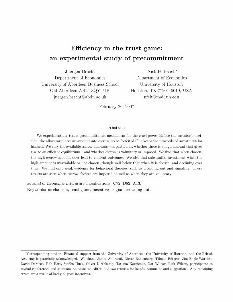
The games we consider are all variants of the basic trust game shown in Figure 1. The investor has twounits of money that she can either invest or not invest; investing a partial amount is not possible. If shedoes not invest, the game ends, she keeps her money, and the allocator gets nothing. If she invests, hermoney quadruples in amount and becomes property of the allocator. The allocator then decides whetherto split these returns evenly with the investor or keep it all for himself; other divisions are not possible.

3

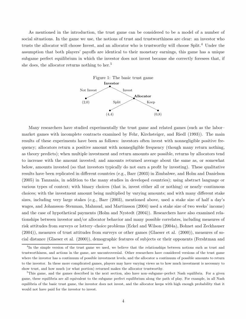
As mentioned in the introduction, the trust game can be considered to be a model of a number ofsocial situations. In the game we use, the notions of trust and trustworthiness are clear: an investor whotrusts the allocator will choose Invest, and an allocator who is trustworthy will choose Split.4 Under theassumption that both players’ payoffs are identical to their monetary earnings, this game has a uniquesubgame perfect equilibrium in which the investor does not invest because she correctly foresees that, ifshe does, the allocator returns nothing to her.5

Figure 1: The basic trust gamesInvestor������

Not InvestHHHHHH

Invests(2,0)

sAllocator������

Splits(4,4)

HHHHHH

Keep s(0,8)

Many researchers have studied experimentally the trust game and related games (such as the labor–market games with incomplete contracts examined by Fehr, Kirchsteiger, and Riedl (1993)). The mainresults of these experiments have been as follows: investors often invest with nonnegligible positive fre-quency; allocators return a positive amount with nonnegligible frequency (though many return nothing,as theory predicts); when multiple investment and return amounts are possible, returns by allocators tendto increase with the amount invested; and amounts returned average about the same as, or somewhatbelow, amounts invested (so that investors typically do not earn a profit by investing). These qualitativeresults have been replicated in different countries (e.g., Barr (2003) in Zimbabwe, and Holm and Danielson(2005) in Tanzania, in addition to the many studies in developed countries); using abstract language orvarious types of context; with binary choices (that is, invest either all or nothing) or nearly–continuouschoices; with the investment amount being multiplied by varying amounts; and with many different stakesizes, including very large stakes (e.g., Barr (2003), mentioned above, used a stake size of half a day’swages, and Johansson–Stenman, Mahmud, and Martinsson (2004) used a stake size of two weeks’ income)and the case of hypothetical payments (Holm and Nystedt (2004)). Researchers have also examined rela-tionships between investor and/or allocator behavior and many possible correlates, including measures ofrisk attitudes from surveys or lottery–choice problems (Eckel and Wilson (2004a), Bohnet and Zeckhauser(2004)), measures of trust attitudes from surveys or other games (Glaeser et al. (2000)), measures of so-cial distance (Glaeser et al. (2000)), demographic features of subjects or their opponents (Fershtman and

4In the simple version of the trust game we used, we believe that the relationships between notions such as trust and

trustworthiness, and actions in the game, are uncontroversial. Other researchers have considered versions of the trust game

where the investor has a continuum of possible investment levels, and the allocator a continuum of possible amounts to return

to the investor. In these more complicated games, players may have varying views as to how much investment is necessary to

show trust, and how much (or what portion) returned makes the allocator trustworthy.5This game, and the games described in the next section, also have non–subgame–perfect Nash equilibria. For a given

game, these equilibria are all equivalent to the subgame perfect equilibrium along the path of play. For example, in all Nash

equilibria of the basic trust game, the investor does not invest, and the allocator keeps with high enough probability that it

would not have paid for the investor to invest.

4

Gneezy (2001), Eckel and Wilson (2002, 2004b), Croson and Buchan (1999)), opponents’ facial expressions(Scharlemann et al. (2001), Eckel and Wilson (2004b)), political ideology and political–party identification(Anderson, Mellor, and Milyo (2004)), finite versus indefinite repetition of the game (Engle–Warnick andSlonim (2004)), experience playing the game (Engle–Warnick and Slonim (2004)), whether the game isin normal– or extensive–form representation (Deck (2001)), and elicitation and/or transmission of beliefsabout opponent’s play (Guerra and Zizzo (2004)).

2.1 The escrow mechanism

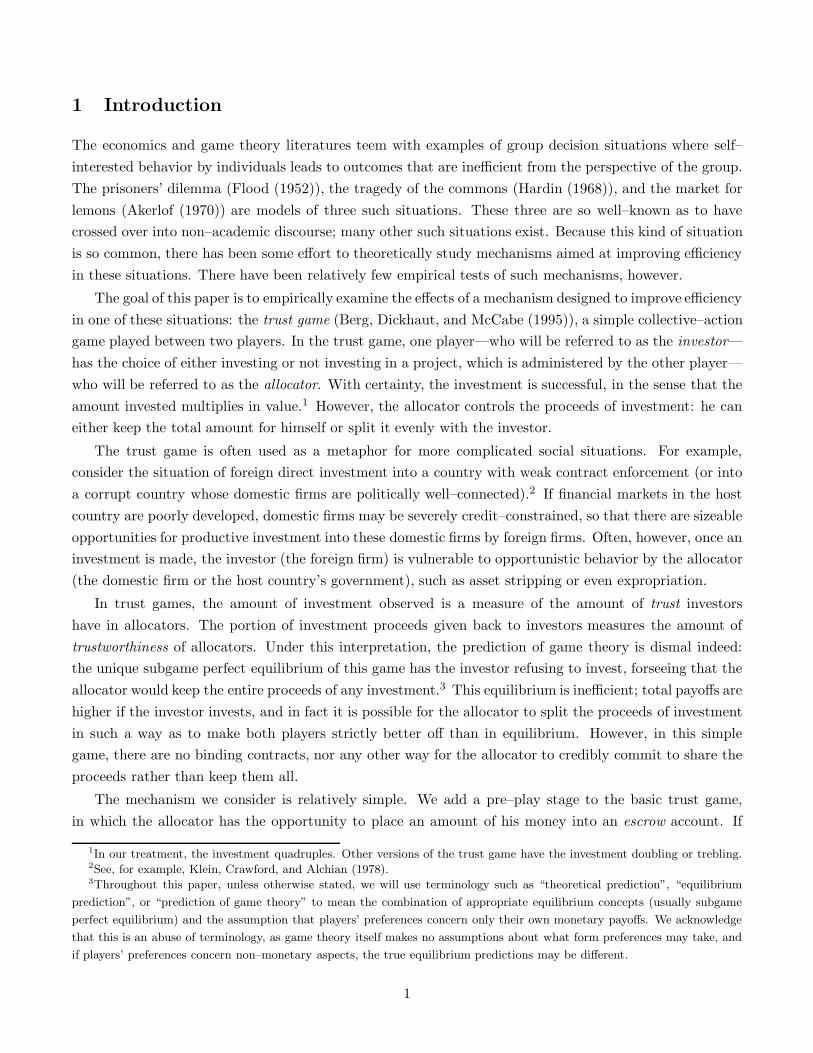
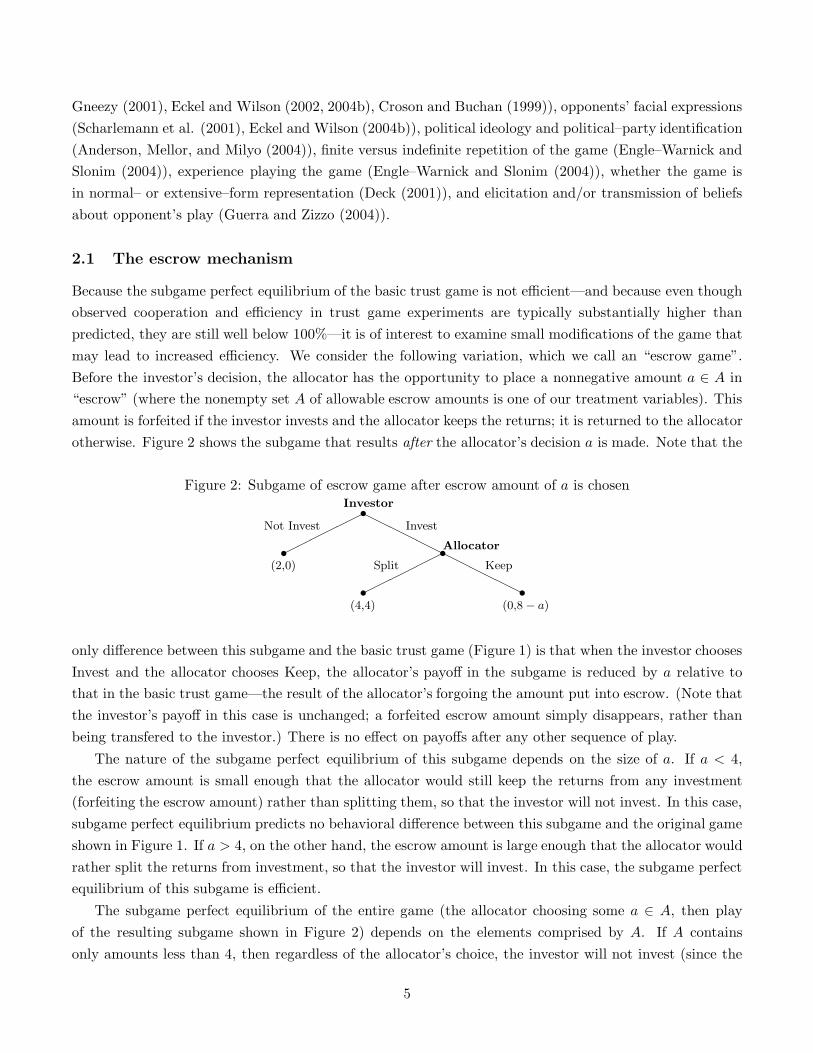
Because the subgame perfect equilibrium of the basic trust game is not efficient—and because even thoughobserved cooperation and efficiency in trust game experiments are typically substantially higher thanpredicted, they are still well below 100%—it is of interest to examine small modifications of the game thatmay lead to increased efficiency. We consider the following variation, which we call an “escrow game”.Before the investor’s decision, the allocator has the opportunity to place a nonnegative amount a ∈ A in“escrow” (where the nonempty set A of allowable escrow amounts is one of our treatment variables). Thisamount is forfeited if the investor invests and the allocator keeps the returns; it is returned to the allocatorotherwise. Figure 2 shows the subgame that results after the allocator’s decision a is made. Note that the

Figure 2: Subgame of escrow game after escrow amount of a is chosensInvestor������

Not InvestHHHHHH

Invests(2,0)

sAllocator������

Splits(4,4)

HHHHHH

Keep s(0,8 − a)

only difference between this subgame and the basic trust game (Figure 1) is that when the investor choosesInvest and the allocator chooses Keep, the allocator’s payoff in the subgame is reduced by a relative tothat in the basic trust game—the result of the allocator’s forgoing the amount put into escrow. (Note thatthe investor’s payoff in this case is unchanged; a forfeited escrow amount simply disappears, rather thanbeing transfered to the investor.) There is no effect on payoffs after any other sequence of play.

The nature of the subgame perfect equilibrium of this subgame depends on the size of a. If a < 4,the escrow amount is small enough that the allocator would still keep the returns from any investment(forfeiting the escrow amount) rather than splitting them, so that the investor will not invest. In this case,subgame perfect equilibrium predicts no behavioral difference between this subgame and the original gameshown in Figure 1. If a > 4, on the other hand, the escrow amount is large enough that the allocator wouldrather split the returns from investment, so that the investor will invest. In this case, the subgame perfectequilibrium of this subgame is efficient.

The subgame perfect equilibrium of the entire game (the allocator choosing some a ∈ A, then playof the resulting subgame shown in Figure 2) depends on the elements comprised by A. If A containsonly amounts less than 4, then regardless of the allocator’s choice, the investor will not invest (since the

5

allocator would keep any returns from investment). Since any escrow choice by the allocator leads to thesame payoffs, subgame perfect equilibrium doesn’t predict which escrow choice he will make. If A containsany amount(s) greater than 4, however, the allocator will choose some such amount, the investor will invest,and the allocator will split. Since any escrow choice above 4 gives the allocator the same payoff, subgameperfect equilibrium again does not predict which such choice he will make.

2.2 Literature and implications

Several other researchers have looked experimentally at mechanisms for improving outcomes in games wherethe equilibrium is inefficient. Many of these mechanisms have been designed specifically for collective–actionproblems. One of the simplest such “mechanisms” involves nothing more than changing the order of play.Van Huyck, Battalio, and Walters (1995) did just this, in an experiment using the peasant–dictator game,which is very similar to the trust game. (See also Walters (1993).) In the usual version, the peasant firstchooses how much to invest into a productive investment, then the dictator chooses what portion of theproceeds to take—so that the peasant and dictator correspond to the investor and allocator in the trustgame. The order of play was varied in the experiment, so that sometimes the dictator chose first, whichis strategically equivalent to giving the dictator a way of credibly committing to a “tax rate” which isobserved by the peasant prior to the investment choice. Van Huyck, Battalio, and Walters found thataverage payoffs for both the peasant and the dictator were much higher when the dictator chose first thanwhen the investor chose first, as game theory predicts.

Andreoni and Varian (1999) examine the ability of a “compensation mechanism” (analyzed by Varian(1994)) to facilitate cooperation. In their experiment, subjects play 15 rounds of an asymmetric prisoners’dilemma, then 25 rounds of a modified version of the game in which, prior to play, each player chooseshow much to offer her opponent in exchange for cooperating, and then each player is told what she hasbeen offered to cooperate. This mechanism changes the equilibrium prediction to one in which bothplayers cooperate (along with suitable compensations in the pre–play stage). However, Andreoni andVarian’s results were mixed. They did find, as predicted, that cooperative behavior was higher underthe mechanism than without it. However, the increase in cooperative behavior was much smaller thanpredicted: cooperation was higher than predicted without the mechanism, but lower than predicted withthe mechanism. It is not clear why cooperation under the mechanism was so low; even following choiceslarge enough to induce cooperation in equilibrium, the frequency of cooperation was only about 70%. Itis worth keeping their results in mind, as their mechanism is similar in nature to the escrow mechanismwe use (the main difference is that their mechanism involves players making decisions that change eachother’s incentives, while ours involves a player changing his own incentives).

Houser et al. (2004) designed a trust game experiment involving a mechanism that is similar in someways to Andreoni’s. Along with choosing an investment amount, investors choose a desired amount to bereturned to them by allocators, and threaten punishment if the allocator returns less than that amount.(Thus, they also have players making decisions that change their counterparts’ incentives, but in thiscase, they are punishments rather than rewards.) They found that when no sanctions were threatened,allocators typically returned a positive amount—though less than the investor requested. When sanctions

6

were threatened, allocator behavior depended on the severity of the sanctions: strong sanctions led toallocators returning the amount requested (though not more), while weak sanctions often led to nothing atall being returned. Interestingly, their results were robust to whether the threat was made by the investoror randomly by the experiment computer program.

Houser et al.’s main results are consistent with crowding out, a pattern of behavior often found incollective–action problems (including the trust game). Ostrom (2000), summarizing a large body of researchon collective–action problems, found (among other empirical regularities) that (1) in situations like ourbasic trust game, levels of cooperative behavior are substantially higher than would be predicted by gametheory, but (2) when rules are added to the game in an attempt to motivate cooperative behavior, peopleact approximately as game theory predicts. Together, these results imply that “externally imposed rulestend to ‘crowd out’ endogenous cooperative behavior” (p. 147).6 In the next section, we will discuss theimplications of crowding out in regards to our own experiment.

Andreoni (2005) considered several versions of a “satisfaction guaranteed” mechanism, added on tothe trust game. Using our terminology, this mechanism allows the investor—after seeing the allocator’sdecision—to choose whether to accept the current outcome or, instead, to impose default payoffs equal tothose the players would have gotten had there been no investment. Andreoni’s experiment had a controltreatment (a basic trust game with no satisfaction–guaranteed option), a treatment where the satisfaction–guaranteed mechanism was imposed on the players, another treatment (“optional guarantee”) where theallocator chose whether to offer the guarantee to the investor, and a fourth treatment (“nonbinding guar-antee”) that was similar to the optional–guarantee treatment, except that the allocator was not forcedto honor his guarantees.7 He found several noteworthy results. As theory predicts, the highest levels ofinvestment and returns were seen following the offer of a binding guarantee—irrespective of whether theoffer was mandatory or made voluntarily. Surprisingly, investment and returns were also high when anonbinding guarantee was offered, though not as high as when the guarantee was binding. Investment andreturns in the basic trust game were comparable to those in other trust games, but the lowest levels ofinvestment and returns were seen in cases where the allocator was allowed to offer a guarantee (binding ornonbinding), but chose not to.

Falkinger et al. (2000) considered a “tax–subsidy mechanism” (proposed by Falkinger (1996)) in whicha third party—such as a government—sets a tax/subsidy rate before the players choose their contributionstoward a public good. After contributions are chosen, players are rewarded or fined according to theirdeviation from the mean contribution level; players making above–average contributions are rewardedproportionally to how far above average their contributions were, and those making below–average contri-

6Lazzarini, Miller, and Zenger (2004) discuss some of the more recent research on crowding out, including experiments in

which crowding out did not occur. They also present the results of their own experiment, in which crowding out does not

occur. They conclude that under some circumstances, formal mechanisms can actually be complements to informal social

norms, rather than substitutes, as crowding out implies.7Andreoni’s mechanism is very similar in nature, though not identical, to the one we examine. One difference is that

Andreoni’s mechanism adds an additional decision for the investor after the allocator chooses an allocation, while our escrow

mechanism does not. Also, when the allocator forgoes a positive escrow amount, that amount is simply lost, with none of it

going to the investor; on the other hand, an investor invoking a satisfaction–guaranteed pledge does raise her payoff whenever

the allocator returned less than the investor invested.

7

butions are punished in a similar way.8 Falkinger et al. (2000) designed an experiment in which subjectsplayed public–good games under several parameterizations (they varied the number of players, the produc-tion function for the public good, players’ incomes and marginal rates of substitution between the publicand private goods, and the tax/subsidy rate). Depending on the treatment, subjects played either 10 or 20rounds of a basic public–good game with no mechanism followed by the same number of rounds with themechanism, or either 10 or 20 rounds with the mechanism followed by the same number of rounds withoutit. They found that cooperative behavior—and therefore, provision of the public good—was substantiallyhigher with the mechanism than without it, but again, the difference was less than the equilibrium predic-tion. Subjects contributed much more than predicted in the basic public–good game (that is, without themechanism), but either less than predicted (when the predicted contribution level was the player’s entireincome, and thus the maximum of the strategy set) or roughly as much as predicted (when the predictedcontribution level was less than the player’s income, and thus in the interior of the strategy set) when themechanism was present.

Bracht, Figuieres, and Ratto (2004) extended the work of Andreoni and Varian (1999) and Falkingeret al. (2000), by more directly comparing the two mechanisms studied by them. The game they used wasa two–player public–good game with utility linear in the public good and concave in the private good,so that both the Nash equilibrium and the joint–payoff–maximizing outcome were in the interior of thestrategy set (both for the basic game and under each mechanism). Subjects in the experiment played 20rounds of this basic public–good game, then 20 rounds of a game with one of the two mechanisms. Bracht,Figuieres, and Ratto found that both mechanisms led to increased cooperative behavior, but the increaseswere smaller than predicted. When there was no mechanism, contributions were consistently above theequilibrium level (though they moved toward it over time). Under the tax–subsidy mechanism, similarly,contributions started above the equilibrium level but reached it by the end of the session. Under thecompensation mechanism, however, contributions started at the equilibrium level but decreased over timeuntil ending well below it (though still higher than without the mechanism).

The results of these six experiments are largely consistent with each other, and carry two implicationsfor us. First, the performance of these mechanisms seems to be relatively robust to small changes inexperimental parameters and procedures. Second, there is substantial crowding out: while cooperativebehavior is well above equilibrium levels when no mechanism is in place, under any of these mechanisms,levels of cooperation are usually no higher, and indeed are often lower, than the equilibrium prediction.Thus, when a weak externally–imposed rule does not change the equilibrium prediction, the result isa decrease in cooperative behavior under the rule compared to when no rule was present. The onlyexception is in Andreoni’s (2005) experiment, where both investment and returns were higher after theallocator offered a nonbinding guarantee (a weak externally–imposed rule) than in the basic trust game.9

Rather, this result is consistent with a signaling hypothesis: in a treatment where no binding guaranteesare possible, the choice of a nonbinding guarantee rather than no guarantee at all is read (correctly, on

8Falkinger (2004) extends his previous model by adding an earlier stage in which players invest in an enforcement technology,

which determines the effective tax/subsidy rate for the second stage.9However, the very low levels of investment and returns when the allocator chose not to offer a guarantee in Andreoni’s

experiment are consistent with crowding out.

8

average) by investors to be a signal of future cooperation—even though this choice does not entail a crediblecommitment in the game–theoretic sense.

2.3 Experimental design and hypotheses

In our experiment, we consider five treatments, differing in A—the set of possible a—as well as howthe escrow decision is made. In our control treatment, no escrow is possible, so that A = {0}. In our“Escrow03” treatment, we set A = {0, 3}, and in our “Escrow036” treatment, A = {0, 3, 6}. In addition,there are two “forced escrow” treatments, where a third party (the computer program) determines theescrow amount, rather than the allocator making the choice. These treatments parallel our Escrow03 andEscrow036 treatments; in our “Forced03” treatment, we again have A = {0, 3}, and in our “Forced036”treatment, A = {0, 3, 6}. (We will sometimes refer to the Escrow03 and Escrow036 treatments as our“voluntary escrow” treatments in contrast.) A summary of the treatments and corresponding subgameperfect equilibrium predictions is shown in Table 1; also shown is a measure of efficiency, which we defineas the sum of investor and allocator payoffs, normalized so that 0 and 1 represent the minimum andmaximum efficiencies. Notice that from a game–theoretic standpoint, the only determinant of investmentand splitting is the amount placed into escrow; whether the escrow choice was voluntary or forced doesnot matter, nor does the existence of larger or smaller alternative escrow choices.

Table 1: Treatments and game–theoretic predictions

Treatment Escrow Probability Conditional Conditional Efficiencyamount chosen Prob(Invest) Prob(Split)

Control 0 1 0 0 0Escrow03 0 * 0 0 0

3 * 0 0 00 0 0 0 0

Escrow036 3 0 0 0 06 1 1 1 1

Forced03 0 — 0 0 03 — 0 0 00 — 0 0 0

Forced036 3 — 0 0 06 — 1 1 1

∗: Either escrow amount can be chosen in subgame perfect equilibrium.

The pre–play escrow stage is an example of a mechanism designed to improve efficiency. As discussedabove, according to subgame perfect equilibrium, this mechanism should work if and only if an escrowamount larger than 4 is chosen. This is possible in the Escrow036 and Forced036 treatments, but not inthe Control treatment (where there is no escrow at all), nor in the Escrow03 and Forced03 treatments

9

(where the escrow amounts are too small). This implies that when the escrow amount is 6, investors willchoose Invest and allocators will choose Split, whereas when the escrow amount is 0 or 3, they will not.This implies the following hypotheses.

Hypothesis 1 The frequency of Invest will be higher following an escrow amount of 6 than following anescrow amount of 0 or 3.

Hypothesis 2 The frequency of Split will be higher following an escrow amount of 6 than following anescrow amount of 0 or 3.

Hypothesis 3 The frequency of Invest will be the same following an escrow amount of 0 as following anescrow amount of 3.

Hypothesis 4 The frequency of Split will be the same following an escrow amount of 0 as following anescrow amount of 3.

While the game–theoretic prediction of the impact of the escrow mechanism is clear, there is somereason to think the actual impact might be different. As mentioned in the previous section, “crowdingout” is often seen in games like our trust game. While the notion of crowding out is sufficiently broadthat multiple interpretations may be possible for some games, we consider the following interpretation forour experimental design. Our Control, Escrow03 (and Forced03), and Escrow036 treatments correspond,respectively, to the three cases that can occur: (1) no externally–imposed rules, (2) weak externally–imposed rules, and (3) strong externally–imposed rules. In our Control treatment—where no externalrules are imposed—levels of investment and splitting (cooperative play) ought to be substantially higherthan game theory predicts. In the other four treatments, levels of investment and splitting ought to besimilar to the game–theoretic prediction, but the prediction itself will depend on the strength of the rules.In our Escrow036 treatment, the rules are strong enough to make cooperative behavior rational (in thesense of maximizing monetary payoffs), so there should be high levels of investment and splitting. In ourEscrow03 and Forced03 treatments, where rules are in place, but they are not strong enough to makecooperative behavior rational, levels of investment and splitting should be as game theory predicts. Notingthat the game–theoretic prediction for the Escrow03 and Forced03 treatments is the same as that for theControl treatment, and that as mentioned above, actual levels for the latter should be higher than thegame–theoretic prediction, the implication is that levels of investment and splitting should actually be evenless in the Escrow03 and Forced03 treatments than in the Control treatment. In the Forced036 treatment,externally–imposed rules are either strong or weak, depending on whether the escrow amount imposed is6 or less than 6. In either case, levels of investment and splitting should be as game theory predicts: high(as in the Escrow036 treatment) when the escrow amount is 6, and low (as in the Escrow03 and Forced03treatments) when the escrow amount is either 0 or 3.

Thus, the “crowding out” hypothesis implies that Hypotheses 1 and 2 above should still hold, butHypotheses 3 and 4 should be replaced by:

Hypothesis 5 The frequency of Invest will be higher in the Control treatment than in each of the othertreatments following an escrow amount of 0 or 3.

10

Hypothesis 6 The frequency of Split will be higher in the Control treatment than in each of the othertreatments following an escrow amount of 0 or 3.

An alternative “signaling” theory makes almost the opposite prediction. According to this theory,allocators who intend to Split will signal their cooperative intention by placing the maximum possibleamount into escrow, thus making it more costly to Keep later (if the investor invests). In the Controland forced–escrow treatments, there is no opportunity for signaling, and in the Escrow036 treatment, theimplication of such signaling is no different from what equilibrium predicts. In the Escrow03 treatment,however, such signaling would imply that an escrow choice of 3 would lead to more cooperative behavior:investors will anticipate that allocators intend to choose Split, so they will choose Invest.

This reasoning implies that other things equal, cooperative behavior should be more likely when theescrow amount chosen by the allocator was the largest escrow amount possible—and of course, that thisamount was actually chosen by the allocator, not imposed externally. This leads to the following hypotheses(in addition to Hypotheses 1 and 2 above):

Hypothesis 7 In the Escrow03 treatment, the frequency of Invest will be higher following an escrow choiceof 3 than following an escrow choice of 0.

Hypothesis 8 In the Escrow03 treatment, the frequency of Split will be higher following an escrow choiceof 3 than following an escrow choice of 0.

Hypothesis 9 Following an escrow choice of 3, the frequency of Invest will be higher in the Escrow03treatment than in the Escrow036, Forced03, or Forced036 treatments.

Hypothesis 10 Following an escrow choice of 3, the frequency of Split will be higher in the Escrow03treatment than in the Escrow036, Forced03, or Forced036 treatments.

3 Experimental procedures

Our design is made up of five treatments, as listed in Table 1 above. In all experimental sessions, subjectsstarted by playing 5 rounds of the basic trust game, with no escrow possible. This was intended tofamiliarize subjects with the strategic situation and the computer interface. After the first 5 rounds werecompleted, subjects played 10 rounds of a game that depended on the treatment. In the Control treatment,these next 10 rounds were also of the basic trust game; in the remaining treatments, these 10 rounds wereof the corresponding game (for example, the Escrow03 game in our Escrow03 treatment).10 All subjects inan experimental session played the same game. Each session involved 20 subjects, with the exception of oneControl session that had only 18 subjects and one Escrow036 session that had only 10 subjects. Subjectswere primarily undergraduate students from University College London and Exeter University, and wererecruited by a variety of methods, including physically posted announcements, postings to a university

10Note here the distinction we draw between game and treatment in our nomenclature. Each treatment begins with 5 rounds

of the basic trust game, then is followed by 10 rounds of a game—possibly the trust game again (in the Control treatment),

and possibly one of the four other games (in each case, in the treatment of the same name).

11

experiments website, and via a database of participants in previous experiments and others expressinginterest in participating in experiments. No one took part in more than one session of this experiment.

At the beginning of a session, each subject was seated in a single room and given a set of writteninstructions for the first five rounds.11 At this point, the subjects were not told how (or if) the game woulddiffer in the last ten rounds, though the instructions did state that these five rounds made up the first partof the experiment, that the second part might be different, and that the rules for the second part wouldbe discussed after the first part ended. The instructions for the first part were read aloud to the subjects,in an attempt to make the rules of the game common knowledge. After the fifth round of a session wascompleted, each subject was given a copy of the instructions for the remaining ten rounds. These werealso read aloud, after which the remaining ten rounds were played.

The experiment was run on networked computer terminals, using the z–Tree experiment softwarepackage (Fischbacher (1999)). Subjects were asked not to communicate with other subjects, so the onlyinteractions were via the computer program. Subjects were randomly assigned to roles (investor or al-locator) at the beginning of a session and remained in the same role throughout the session. Investorsand allocators were matched using a round–robin matching format; in rounds 1–5, each investor wouldbe matched to each allocator at most once (and vice versa), and in rounds 6–15, each investor would bematched to each allocator exactly once.12

In a round of the basic trust game (either in those sessions where it was played for all 15 rounds,or in the first 5 rounds of the other sessions), investors were prompted to choose whether they wouldInvest or Not Invest their 2 units. After the investors’ choices were entered, each allocator would seehis counterpart’s decision; if it was Invest, the allocator would then be prompted to choose whether hewould Split or Keep. After the allocators had entered their decisions, all subjects received feedback fromthe just–completed round: the investor’s choice, the allocator’s choice (if the investor chose Invest), andthe subject’s own payoff. Subjects were not explicitly told their counterparts’ payoffs, though they weregiven enough information to be able to calculate them easily if they wished. Subjects were not given anyinformation about the results of other pairs of subjects.

In a round of either the Escrow03 or the Escrow036 game (rounds 6–15 of the corresponding treatments),the sequence of play was similar, except for the escrow decision. In these treatments, a round would beginwith allocators’ being prompted to choose which of the allowable escrow amounts would be placed intoescrow. Each investor would see her counterpart’s decision before making her investment decision. Afterinvestment decisions were entered, allocators received this information as in the basic trust game and werethen prompted to choose whether to Split or Keep. In the Forced03 and Forced036 games, the sequenceof play was identical, except that allocators did not choose the escrow amounts, but rather were informedof them at the same time investors were. The computer program chose each possible escrow amount

11One set of instructions—those used for the Escrow03 treatment—are in the appendix to this paper. The instructions used

for other treatments in the experiment, as well as the raw data, are available from the corresponding author upon request.12An implication of this matching mechanism is that over a fifteen–round session, subjects would be matched with some

other subjects more than once. We tried to reduce the possibility that this would lead to repeated–game effects by not telling

subjects the ID number of their counterparts, so that in the last ten rounds, each only knew that with positive probability,

their current counterpart was someone with whom they were matched earlier.

12

with roughly equal frequency.13 Subjects’ feedback at the end of a round in each of the voluntary– andforced–escrow treatments was as in the basic trust game, with the addition of the escrow amount. In alltreatments, at the end of a round, subjects were asked to observe their result, write the information fromthat round down in a record sheet, and then click a button to continue to the next round.

At the end of round 15 of any treatment, the experimental session ended. All subjects received a £5show–up fee.14 In addition, one of the first five rounds and one of the last ten rounds were randomly chosen,and each subject received his/her earnings from these two rounds, at an exchange rate of £1 per point.Subjects earned an average of about £10 for participating in a session, which typically lasted between 30and 45 minutes.

4 Experimental results

The experiment consisted of a total of fifteen sessions, three of each treatment. We begin our discussionof the results by presenting summary statistics concerning aggregate behavior in each of our treatments.Later, we will look at round–by–round behavior, and examine estimation results based on parametricmodels.

4.1 Session aggregates

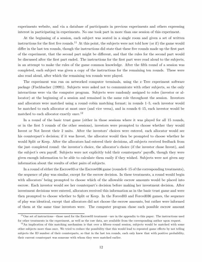
Some features of the aggregate data are shown in Tables 2 and 3. Table 2 shows the relative frequencies ofInvest choices by investors in the first five rounds (when subjects were playing the basic trust game in allsessions), the conditional relative frequencies of Split choices by allocators (given Invest) in these rounds,and the payoff efficiency (as in Table 1, the average joint payoff, normalized so that the maximum possibleefficiency is one and the minimum possible is zero).15 This table also shows the levels of investment,splitting, and efficiency broken down by treatment. Since subjects were playing the same game in theserounds, regardless of the treatment (differences in the game across treatments didn’t begin until round 6),and at this stage had not been given any information as to how, if at all, the second part of the experimentwould differ from the first, any differences observed across treatments here could be construed as beingdue to random variation in trust or trustworthiness across individual subjects (and perhaps other subjectsreacting to this).

Behavior in the first five rounds is substantially different from the subgame perfect equilibrium pre-diction, as Table 2 shows: both Invest and Split do occur with nonnegligible frequency. Investors choose

13The assignment of escrow amounts to allocators in each round was determined in advance, rather than being drawn

randomly during the round, so that results would be comparable across sessions. In the Forced03 treatment, the total

numbers of 0 and 3 escrow amounts were equal (a total of 150 occurrences of each). Due to a minor programming error, the

total numbers of 0, 3, and 6 escrow amounts in the Forced036 treatment were not exactly the same, but were close (a total of

100, 97, and 103 occurrences, respectively).14At the time of the experiment, £1 was worth roughly $1.80.15When escrow is not possible, efficiency is therefore simply equal to the frequency of Invest choices. We list efficiencies

separately so that one could easily make comparisons with treatments in which escrow is possible and efficiency therefore

depends not only on the frequency of Invest choices, but also on that of Keep choices.

13

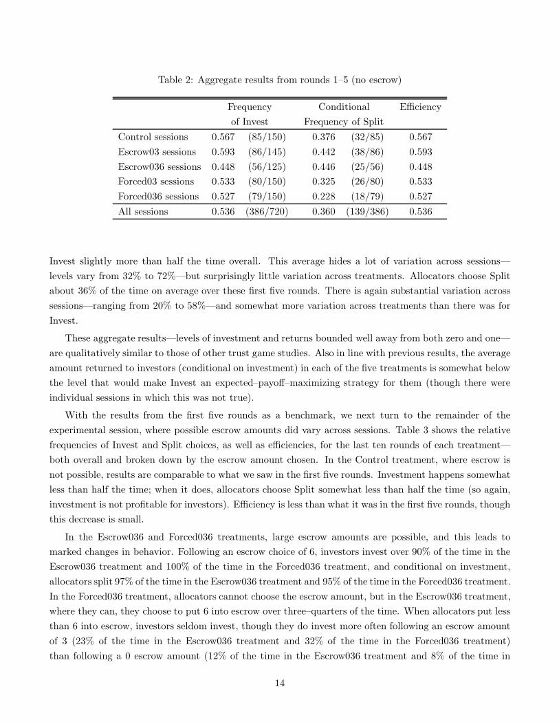
Table 2: Aggregate results from rounds 1–5 (no escrow)

Frequency Conditional Efficiencyof Invest Frequency of Split

Control sessions 0.567 (85/150) 0.376 (32/85) 0.567Escrow03 sessions 0.593 (86/145) 0.442 (38/86) 0.593Escrow036 sessions 0.448 (56/125) 0.446 (25/56) 0.448Forced03 sessions 0.533 (80/150) 0.325 (26/80) 0.533Forced036 sessions 0.527 (79/150) 0.228 (18/79) 0.527All sessions 0.536 (386/720) 0.360 (139/386) 0.536

Invest slightly more than half the time overall. This average hides a lot of variation across sessions—levels vary from 32% to 72%—but surprisingly little variation across treatments. Allocators choose Splitabout 36% of the time on average over these first five rounds. There is again substantial variation acrosssessions—ranging from 20% to 58%—and somewhat more variation across treatments than there was forInvest.

These aggregate results—levels of investment and returns bounded well away from both zero and one—are qualitatively similar to those of other trust game studies. Also in line with previous results, the averageamount returned to investors (conditional on investment) in each of the five treatments is somewhat belowthe level that would make Invest an expected–payoff–maximizing strategy for them (though there wereindividual sessions in which this was not true).

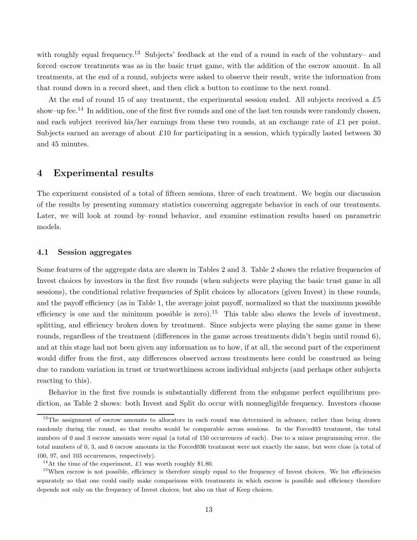
With the results from the first five rounds as a benchmark, we next turn to the remainder of theexperimental session, where possible escrow amounts did vary across sessions. Table 3 shows the relativefrequencies of Invest and Split choices, as well as efficiencies, for the last ten rounds of each treatment—both overall and broken down by the escrow amount chosen. In the Control treatment, where escrow isnot possible, results are comparable to what we saw in the first five rounds. Investment happens somewhatless than half the time; when it does, allocators choose Split somewhat less than half the time (so again,investment is not profitable for investors). Efficiency is less than what it was in the first five rounds, thoughthis decrease is small.

In the Escrow036 and Forced036 treatments, large escrow amounts are possible, and this leads tomarked changes in behavior. Following an escrow choice of 6, investors invest over 90% of the time in theEscrow036 treatment and 100% of the time in the Forced036 treatment, and conditional on investment,allocators split 97% of the time in the Escrow036 treatment and 95% of the time in the Forced036 treatment.In the Forced036 treatment, allocators cannot choose the escrow amount, but in the Escrow036 treatment,where they can, they choose to put 6 into escrow over three–quarters of the time. When allocators put lessthan 6 into escrow, investors seldom invest, though they do invest more often following an escrow amountof 3 (23% of the time in the Escrow036 treatment and 32% of the time in the Forced036 treatment)than following a 0 escrow amount (12% of the time in the Escrow036 treatment and 8% of the time in

14

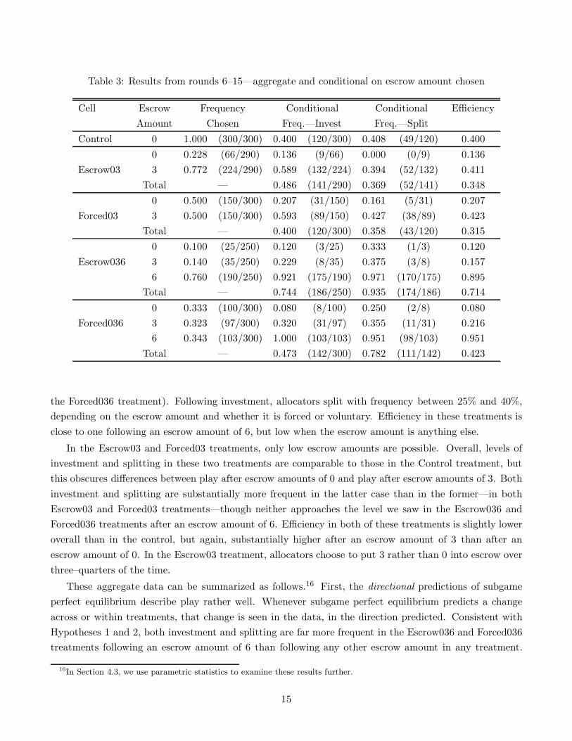
Table 3: Results from rounds 6–15—aggregate and conditional on escrow amount chosen

Cell Escrow Frequency Conditional Conditional EfficiencyAmount Chosen Freq.—Invest Freq.—Split

Control 0 1.000 (300/300) 0.400 (120/300) 0.408 (49/120) 0.4000 0.228 (66/290) 0.136 (9/66) 0.000 (0/9) 0.136

Escrow03 3 0.772 (224/290) 0.589 (132/224) 0.394 (52/132) 0.411Total — 0.486 (141/290) 0.369 (52/141) 0.348

0 0.500 (150/300) 0.207 (31/150) 0.161 (5/31) 0.207Forced03 3 0.500 (150/300) 0.593 (89/150) 0.427 (38/89) 0.423

Total — 0.400 (120/300) 0.358 (43/120) 0.3150 0.100 (25/250) 0.120 (3/25) 0.333 (1/3) 0.120

Escrow036 3 0.140 (35/250) 0.229 (8/35) 0.375 (3/8) 0.1576 0.760 (190/250) 0.921 (175/190) 0.971 (170/175) 0.895

Total — 0.744 (186/250) 0.935 (174/186) 0.714

0 0.333 (100/300) 0.080 (8/100) 0.250 (2/8) 0.080Forced036 3 0.323 (97/300) 0.320 (31/97) 0.355 (11/31) 0.216

6 0.343 (103/300) 1.000 (103/103) 0.951 (98/103) 0.951Total — 0.473 (142/300) 0.782 (111/142) 0.423

the Forced036 treatment). Following investment, allocators split with frequency between 25% and 40%,depending on the escrow amount and whether it is forced or voluntary. Efficiency in these treatments isclose to one following an escrow amount of 6, but low when the escrow amount is anything else.

In the Escrow03 and Forced03 treatments, only low escrow amounts are possible. Overall, levels ofinvestment and splitting in these two treatments are comparable to those in the Control treatment, butthis obscures differences between play after escrow amounts of 0 and play after escrow amounts of 3. Bothinvestment and splitting are substantially more frequent in the latter case than in the former—in bothEscrow03 and Forced03 treatments—though neither approaches the level we saw in the Escrow036 andForced036 treatments after an escrow amount of 6. Efficiency in both of these treatments is slightly loweroverall than in the control, but again, substantially higher after an escrow amount of 3 than after anescrow amount of 0. In the Escrow03 treatment, allocators choose to put 3 rather than 0 into escrow overthree–quarters of the time.

These aggregate data can be summarized as follows.16 First, the directional predictions of subgameperfect equilibrium describe play rather well. Whenever subgame perfect equilibrium predicts a changeacross or within treatments, that change is seen in the data, in the direction predicted. Consistent withHypotheses 1 and 2, both investment and splitting are far more frequent in the Escrow036 and Forced036treatments following an escrow amount of 6 than following any other escrow amount in any treatment.

16In Section 4.3, we use parametric statistics to examine these results further.

15

However, subgame perfect equilibrium’s point predictions often perform poorly; for only a few treatmentsand escrow amounts do we see levels of investment and splitting close to zero. (In the next section, we willsee that subgame perfect equilibrium fares better as a prediction of asymptotic behavior.)

Second, these aggregate data show some evidence of crowding out. Recall that crowding out impliesthat investment and splitting should be less frequent, and efficiency lower, when a weak mechanism isimposed (in the Escrow03 and Forced03 treatments and in the Forced036 treatment following escrow of 0or 3) than when there is no mechanism at all (in the Control treatment). In fact, the overall frequency ofinvestment in all of the weak–mechanism cases is 0.381, the frequency of splitting is 0.360, and efficiencyis 0.273, all lower than their counterpart statistics in the Control treatment (0.400, 0.408, and 0.400,respectively). This difference is fairly substantial for efficiency, but less so for investment and splitting.17

Third, levels of Invest and Split depend not only on how much was put into escrow, but also on whatother escrow choices were available (in contrast to the equilibrium prediction that the availability of otheroptions should be irrelevant). In particular, we see much more investment following a given escrow decisionwhen that was the largest possible escrow amount than when it was not. For an escrow amount of 3, thisis the largest possible escrow amount in the Escrow03 and Forced03 treatments, but a larger amount waspossible in the Escrow036 and Forced036 treatments. Indeed, the frequency of investment following anescrow amount of 3 is 0.589 in the Escrow03 treatment and 0.593 in the Forced03 treatment but only 0.229in the Escrow036 treatment and 0.320 in the Forced036 treatment. For an escrow amount of 0, this isthe largest possible escrow amount in the Control treatment, but a larger amount was possible in each ofthe other four treatments; the subsequent frequency of investment is 0.400 in the Control treatment butranges only from 0.080 to 0.207 in the other treatments. This pattern also holds for allocators, though thedifferences are sometimes small. Following an escrow choice of 3 and investment, allocators choose Splitonly slightly more often in the Escrow03 and Forced03 treatments (0.394 and 0.427, respectively) than inthe Escrow036 and Forced036 treatments (0.375 and 0.355). After an escrow choice of 0 and investment,allocators choose Split more frequently in the Control treatment (0.408) than in any of the other treatments(ranging from 0 to 0.333), though the sample sizes concerned are sometimes small.

Fourth, behavior is largely unaffected by whether escrow decisions are voluntary or forced. There areessentially no apparent qualitative differences in investment, splitting, or efficiency between the Escrow03and Forced03 data, nor between the Escrow036 and Forced036 data, either overall or when broken downby escrow amount. While consistent with subgame perfect equilibrium, this result stands in contrast toother experimental studies which show that behavior can be sensitive to such a manipulation.18

17One might argue that “weak mechanism” could also include those plays in the Escrow036 treatment in which the allocator

chose to put 0 or 3 into escrow. Using this definition changes the weak–mechanism levels of investment, splitting, and efficiency

only slightly—0.367, 0.360, and 0.264 respectively—so that again, efficiency is substantially less than in the Control treatment,

while the difference is small for investment and splitting.18Such sensitivity is most common when the situation is one where nonpecuniary aspects of outcomes are important, as in

the trust game. For example, see Cox and Deck’s (2002) results for allocators in the trust game, or Blount’s (1995) results for

the ultimatum game.

16

4.2 Behavior dynamics

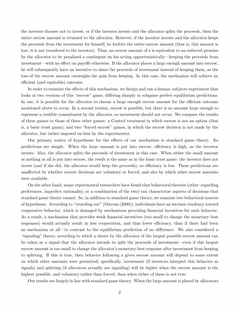
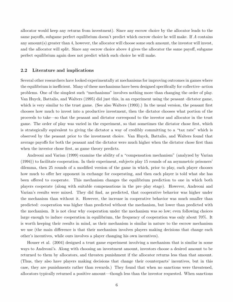
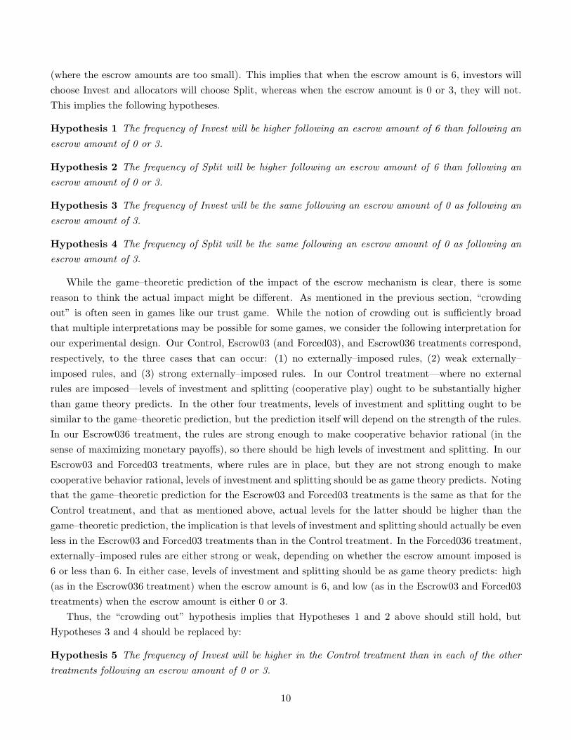
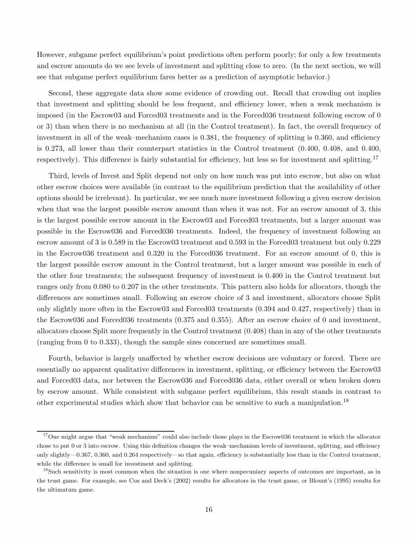
Figure 3 shows the round–by–round relative frequencies of Invest and Split for the Control, Escrow03, andEscrow036 treatments. Note that these frequencies are not broken down by escrow amount. (As mentionedearlier, sample sizes are small for escrow choices less than the maximum possible choice.) Consider first theinitial five rounds, during which there is no escrow. Qualitative dynamics in these rounds are similar in allthree treatments (and as we will see shortly, in the other two treatments as well). The frequency of Investstarts between about two–thirds and three–quarters, but by the fifth round has declined by half or more ineach of the three treatments. The frequency of Split starts at about one–half and drops reasonably steadilyover these five rounds to below 20% in each treatment (and, indeed, to zero in the Control treatment).Since Invest is a monetary best response for the investor only if the probability of Split is at least one–half, it appears that on average, investors are reacting rationally to their experiences of the behavior ofallocators.

Figure 3: Round–by–round unconditional relative frequencies of Invest and Split(Control and voluntary–escrow treatments)

Round

Frequency of Invest by investor Frequency of Split by allocators sc cEscrow036 Escrow036Escrow03 Escrow03Control Control

1 15 56 610 1015 150.0 0.0

0.2 0.2

0.4 0.4

0.6 0.6

0.8 0.8

1.0 1.0

b b bb

b

bb b b b b

b bb

b

r r rr r

rr r r

r r rr r

r

b b

b b b

bb b

bb b b

b bbr r r

rr

r r rr r r

r r r

r

pppppppppppppppppppppppppppppppppppppppppppppppppppppppppppppppppppppppppppppppppppppppppppppppppppppppppppppppppppppppppppppppppppppppppppppppppppppppppppppppppppppppppppppppppppppppppppppppppppppppppppppppppppppppppppppppppppppppppppppppppppppppppppppppppppppppppppppppppppppppppppppppppppppppppppppppppppppppppppppppppppppppppppppppppppppppppppppppppppppppppppppppppppppppppppppppppp

pppppppppppppppppppppppppppppppppppppppppppppppppppppppppppppppppppppppppppppppppppppppppppppppppppppppppppppppppppppppppppppppppppppppppppppppppppppppppppppppppppppppppppppppppppppppppppppppppppppppppppppppppppppppppppppppppppppppppppppppppppppppppppppppppppppppppppppppppppppppppppppppppppppppppppppppppppppppppppppppppppppppppppppppppppppppppppppppppppppppppppppppppppppppppppppppppppppppppppppppppppppppppppppppppppppppppppppppppppppppppppppppppppppppppppppppppppppppppppppppppppppppppppppppppppppppppppppppppppppppppppppppppppppppppppppppppppppppppppppppppppppppppppppppppppppppppppppppppppppppppppppppppppppppppppppppppppppppppppppppppppppppppppppppppppppppppppppppppppppppppppppppppppppppppppppppppppppppppppppppppppppppppppppppppppppppppppppppppppppppppppppppppppppppppppppppppppppppppppppppppppppppppppppppppppppppppppppppppppppppppppppppppppppppppppppppppppppppppppppppppppppppppppppppppppppppppppppp

pppppppppppppppppppppppppppppppppppppppppppppppppppppppppppppppppppppppppppppppppppppppppppppppppppppppppppppppppppppppppppppppppppppppppppppppppppppppppppppppppppppppppppppppppppppppppppppppppppppppppppppppppppppppppppppppppppppppppppppppppppppppppppppppppppppppppppppppppppppppppppppppppppppppppppppppppppppppppppppppppppppppppppppppppppppppppppppppppppppppppppppppppppppppppppppppppppppppppppppppp

ppppppppppppppppppppppppppppppppppppppppppppppppppppppppppppppppppppppppppppppppppppppppppppppppppppppppppppppppppppppppppppppppppppppppppppppppppppppppppppppppppppppppppppppppppppppppppppppppppppppppppppppppppppppppppppppppppppppppppppppppppppppppppppppppppppppppppppppppppppppppppppppppppppppppppppppppppppppppppppppppppppppppppppppppppppppppppppppppppppppppppppppppppppppppppppppppppppppppppppppppppppppppppppppppppppppppppppppppppppppppppppppppppppppppppppppppppppppppppppppppppppppppppppppppppppppppppppppppppppppppppppppppppppppppppppppppppppppppppppppppppppppppppppppppppppppppppppppppppppppppppppppppppppppppppppppppppppppppppppppppppppppppppppppppppppppppppppppppppppppppppppppppppppppppppppppppppppppppppppppppppppppppppppppppppppppppppppppppppppppppppppppppppppppppppppppppppppppppppppppppppppppppppppppppppppppppppppppppppppppppppppppppppppppppppppppppppppppppppppppppppppppppppppppppppppppppppppppppppppppppppppppppppppppppppppppppp

pppppppppppppppppppppppppppppppppppppppppppppppppppppppppppppppppppppppppppppppppppppppppppppppppppppppppppppppppppppppppppppppppppppppppppppppppppppppppppppppppppppppppppppppppppppppppppppppppppppppppppppppppppppppppppppppppppppppppppppppppppppppppppppppppppppppppppppppppppppppppppppppppppppppppppppppppppppppppppppppppppppppppppppppppppppppppppppppppppppppppppppppppppppppppppppppppppppppppppppppppppppppppppppppppppppppppppppppppppppppppppppppppppppppppppppppppppppppppppppppppppppppppppppppppppppppppppppppppppppppppppppppppppppppppppppppppppppp

ppppppppppppppppppppppppppppppppppppppppppppppppppppppppppppppppppppppppppppppppppppppppppppppppppppppppppppppppppppppppppppppppppppppppppppppppppppppppppppppppppppppppppppppppppppppppppppppppppppppppppppppppppppppppppppppppppppppppppppppppppppppppppppppppppppppppppppppppppppppppppppppppppppppppppppppppppppppppppppppppppppppppppppppppppppppppppppp

pppppppppppppppppppppppppppppppppppppppppppppppppppppppppppppppppppppppppppppppppppppppppppppppppppppppppppppppppppppppppppppppppppppppppppppppppppppppppppppppppppppppppppppppppppppppppppppppppppppppppppppppppppppppppppppppppppppppppppppppppppppppppppppppppppppppppppppppppppppppppppppppppppppppppppppppppppppp

pppppppppppppppppppppppppppppppppppppppppppppppppppppppppppppppppppppppppppppppppppppppppppppppppppppppppppppppppppppppppppppppppppppppppppppppppppppppppppppppppppppppppppppppppppppppppppppppppppppppppppppppppppppppppppppppppppppppppppppppppppppppppppppppppppppppppppppppppppppppppppppppppppppppppppppppppppppppppppppppppppppppppppppppppppppppppppppppppppppppppppppppppppppppppppppppppppppppppppppppppppppppppppppppppppppppppppppppppppppppppppppppppppppppppppppppppppppppppppppppppppppppppppppppppppppppppppppppppppppppppppppppppppppppppppppppppppppppppppppppppppppppppppppppppppppppppppppppppppp

pppppppppppppppppppppppppppppppppppppppppppppppppppppppppppppppppppppppppppppppppppppppppppppppppppppppppppppppppppppppppppppppppppppppppppppppppppppppppppppppppppppppppppppppppppppppppppppppppppppppppppppppppppppppppppppppppppppppppppppppppppppppppppppppppppppppppppppppppppppppppppppppppppppppppppppppppppppppppppppppppppppppppppppppppppppppppppppppppppppppppppppppppppppppppppppppppppppppppppppppppppppppppppppppp

pppppppppppppppppppppppppppppppppppppppppppppppppppppppppppppppppppppppppppppppppppppppppppppppppppppppppppppppppppppppppppppppppppppppppppppppppppppppppppppppppppppppppppppppppppppppppppppppppppppppppppppppppppppppppppppppppppppppppppppppppppppppppppppppppppppppppppppppppppppppppppppppppppppppppppppppppppppppppppppppppppppppppppppppppppppppppppppppppppppppppppppppppppppppppppppppppppppppppppppppppppppppppppppppppppppppppppppppppppppppppppppppppppppppppppppppppppppppppppppppppppppppppppppppppppppppppppppppppppppppppppppppppppppppppppp

ppppppppppppppppppppppppppppppppppppppppppppppppppppppppppppppppppppppppppppppppppppppppppppppppppppppppppppppppppppppppppppppppppppppppppppppppppppppppppppppppppppppppppppppppppppppppppppppppppppppppppppppppppppppppppppppppppppppppppppppppppppppppppppppppppppppppppppppppppppppppppppppppppppppppppppppppppppppppppppppppppppppppppppppppppppppppppppppppppppppppppppppppppppppppppppppppppppppppppppppppppppppppppppppppppppppppppppppppppppppp

pppppppppppppppppppppppppppppppppppppppppppppppppppppppppppppppppppppppppppppppppppppppppppppppppppppppppppppppppppppppppppppppppppppppppppppppppppppppppppppppppppppppppppppppppppppppppppppppppppppppppppppppppppppppppppppppppppppppppppppppppppppppppppppppppppppppppppppppppppppppppppppppppppppppppppppppppppppppppppppppppppppppppppppppppppppppppppppppppppppppppppppppppppppppppppppppppppppppppppppppppppppppppppppppppppppppppppppppppppppppppppppppppppppppppppppppppppppppppppppppppppppppppppppppppppppppppppppppppppppppppppppppppppppppppppppppppppppppppppppppppppppppppppppppppppppppppppppppppppppppppppppppppppppppppppppppppppppppppppppppppppppppppppppppppppppppppppppppppppppppppppppppppppppppppppppppppppppppppppppppppppppppppppppppppppppppppppppppppppppppppppppppppppppppppppppppppppppppppppppppppppppppppppppppppppppppppppppppppppppppppppppppppppppppppppppppppppppppppppppppppppppppppppppppppppppppppppppppppppppppppppppppppppppppppppppppppppppppppppppppppppppppppppppppppppppppppppppppppppppppppppppppppppppppppppppppppppppppppppppppppppppppppppppppppppppppppppppppppppppppppppppppppp

ppppppppppppppppppppppppppppppppppppppppppppppppppppppppppppppppppppppppppppppppppppppppppppppppppppppppppppppppppppppppppppppppppppppppppppppppppppppppppppppppppppppppppppppppppppppppppppppppppppppppppppppppppppppppppppppppppppppppppppppppppppppppppppppppppppppppppppppppppppppppppppppppppppppppppppppppppppppppppppppppppppppppppppppppppppppppppppppppppppppppppppppppppppppppppppppppppppppppppppppppppppppppppppppppppppppppppppppppppppppppppppppppppppppppppppppppppppppppppppppppppppppppppppppppppppppppppppppppppppppppppppppppppppppppp

pppppppppppppppppppppppppppppppppppppppppppppppppppppppppppppppppppppppppppppppppppppppppppppppppppppppppppppppppppppppppppppppppppppppppppppppppppppppppppppppppppppppppppppppppppppppppppppppppppppppppppppppppppppppppppppppppppppppppppppppppppppppppppppppppppppppppppppppppppppppppppppppppppppppppppppppppppppppppppppppppppppppppppppppppppppppppppppppppppppppppppppppppppppppppppppppppppppppppppppppppppppppppppppppppppppppppppppppppppppppppppppppppppppppppppppppppppppppppppppppppppppppppppppppppppppppppppppppppppppppppppppppppppppppppppppppppppppppppppppppppppppppppppppppppppppppppppppppppppppppppppppppppppppppppppp

In all treatments, the levels of investment and splitting increase sharply from round 5 to round 6, thefirst round of the second part of the session. In the Escrow036 treatment, the equilibrium predictions forboth investment frequency and splitting frequency go from zero in round 5 to one in round 6, so it is notsurprising to see an increase there. In the other two treatments, the equilibrium predictions are unchangedfrom round 5 to round 6, so it is less clear what causes these increases. In the Control treatment, thereis no change in the rules of the game from round 5 to round 6, so it is likely that the change in levels ofinvestment and splitting is due to a “restart effect”—a change in behavior caused purely by referring toround 6 as the first round of the second part of the session instead of one more round in the first part(see, for example, Andreoni (1988), Moxnes and van der Heijden (2003), Camerer and Fehr (2003), andCroson, Fatas, and Neugebauer (2005)). The cause of the changes in investment and splitting levels in the

17

Escrow03 treatment may be a restart effect, or may have occurred because subjects incorrectly perceivedthat some relevant aspect of the strategic environment has changed.

Dynamics in investor behavior over the last 10 rounds of the Control and Escrow03 treatments arebroadly similar. Investment frequencies start out relatively high—above 60% in both treatments—butdecline over time, though always remaining above zero (the equilibrium prediction). Allocator behaviordiffers somewhat in these two treatments; in the Control treatment, the frequency of Split varies between20% and 60% but shows no time trend, while splitting in the Escrow03 treatment falls from about 50% tozero.

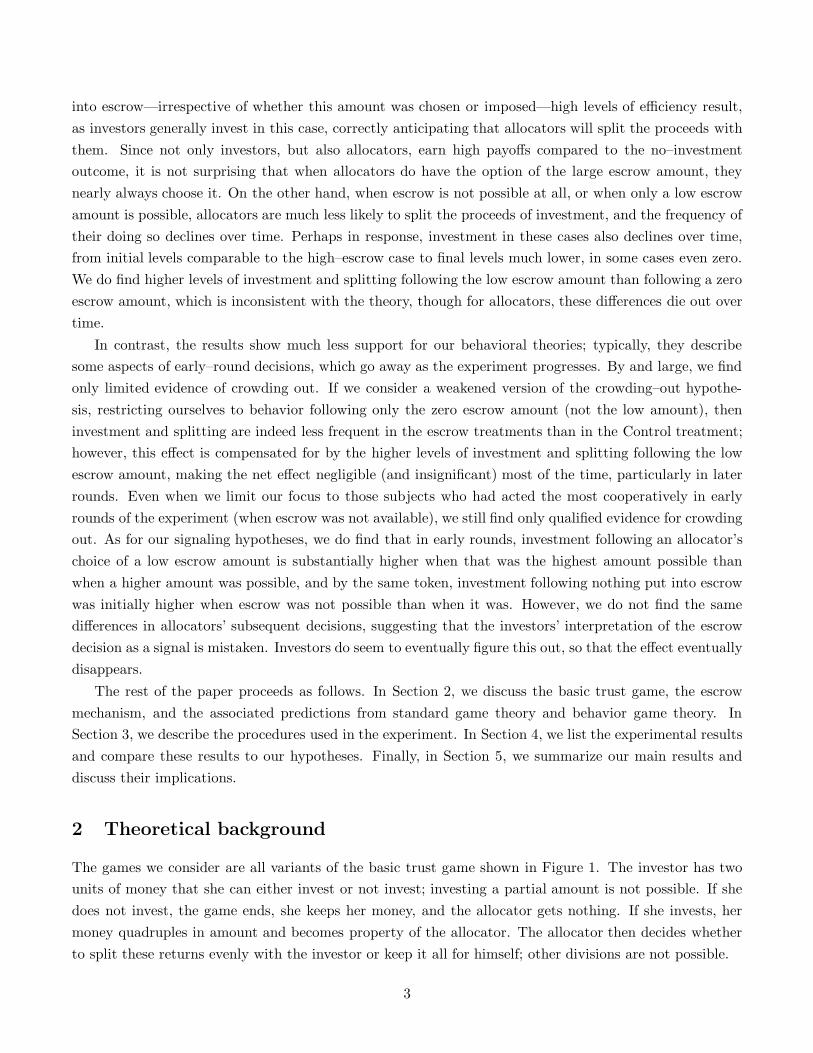
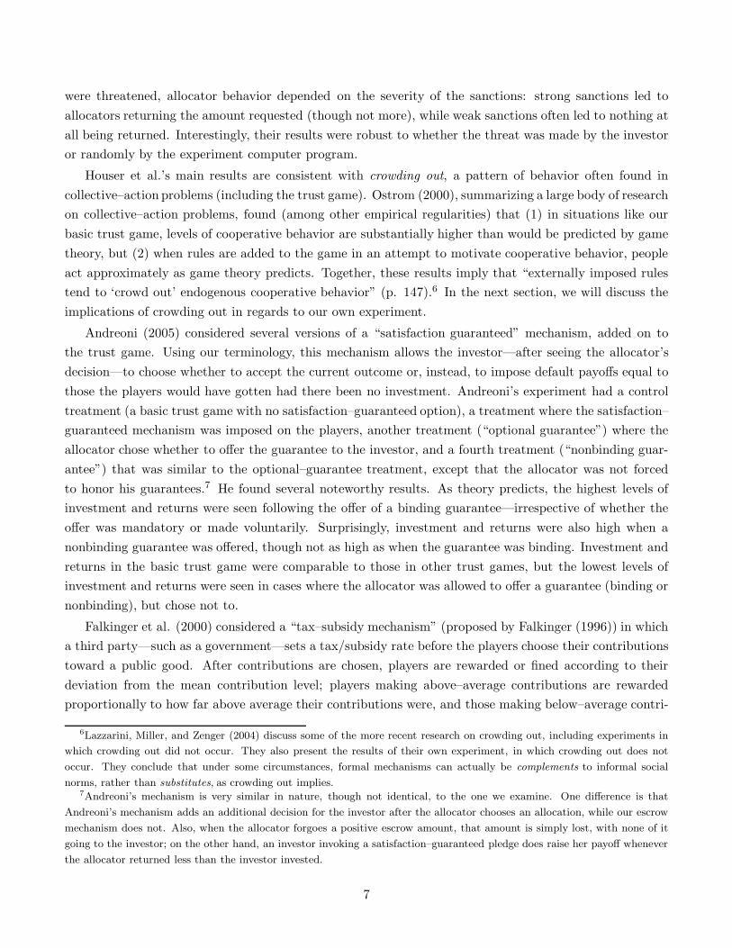
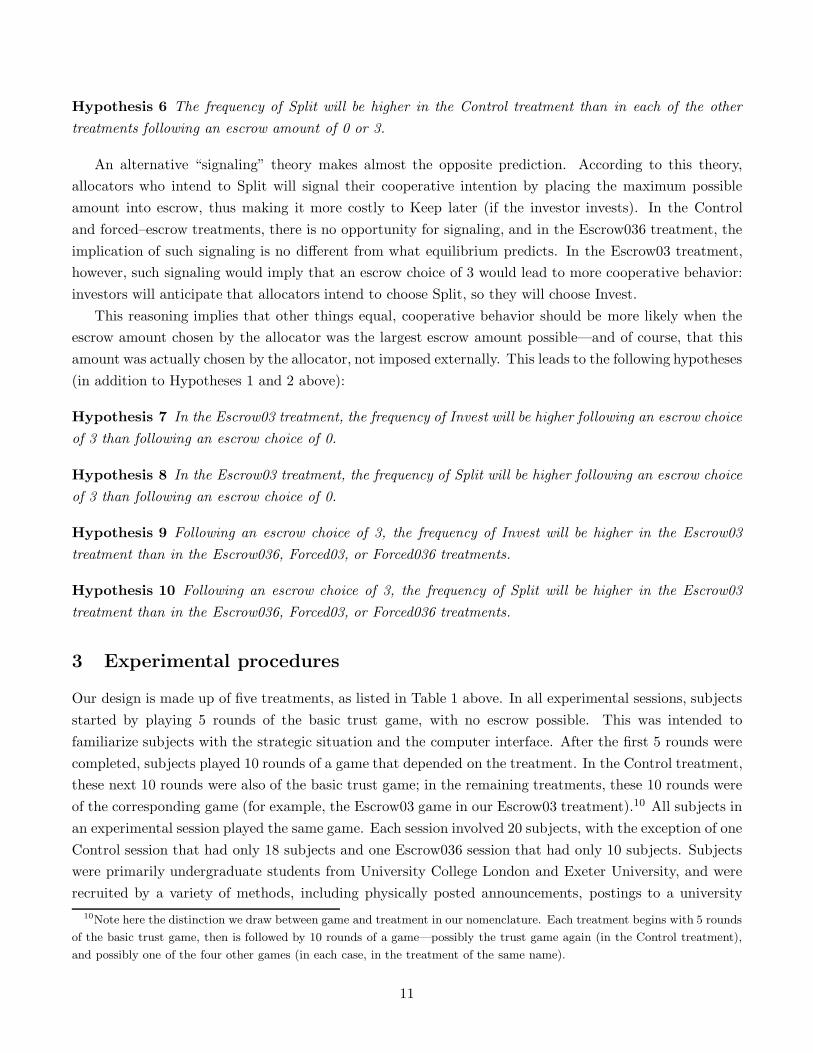
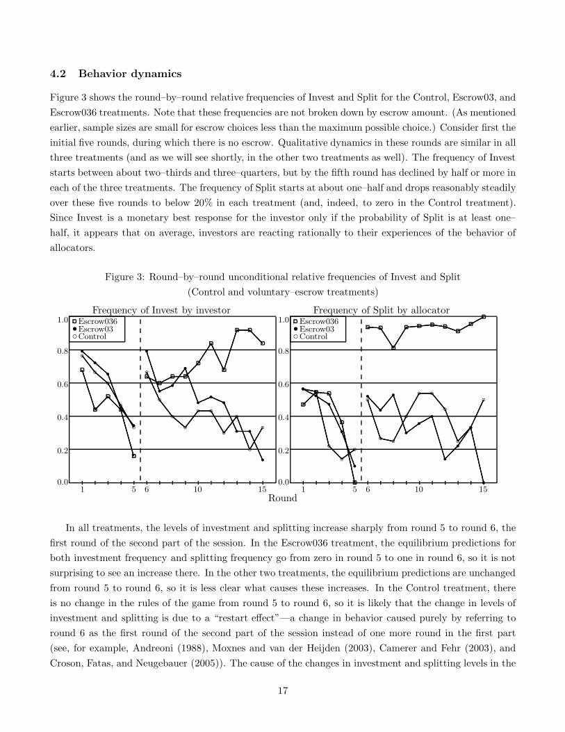
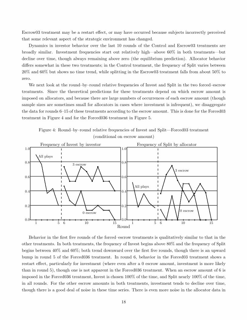
We next look at the round–by–round relative frequencies of Invest and Split in the two forced–escrowtreatments. Since the theoretical predictions for these treatments depend on which escrow amount isimposed on allocators, and because there are large numbers of occurrences of each escrow amount (thoughsample sizes are sometimes small for allocators in cases where investment is infrequent), we disaggregatethe data for rounds 6–15 of these treatments according to the escrow amount. This is done for the Forced03treatment in Figure 4 and for the Forced036 treatment in Figure 5.

Figure 4: Round–by–round relative frequencies of Invest and Split—Forced03 treatment(conditional on escrow amount)

Round

Frequency of Invest by investor Frequency of Split by allocator

All plays

3 escrow

0 escrow

All plays

3 escrow

0 escrow

1 15 56 610 1015 150.0 0.0

0.2 0.2

0.4 0.4

0.6 0.6

0.8 0.8

1.0 1.0pp

p pp

bb b

bb b b b b

b

rr r

r rr

rr r

r

ppppppppppppppppppppppppppppppppppppppppppppppppppppppppppppppppppppppppppppppppppppppppppppppppppppppppppppppppppppppppppppppppppppppppppppppppppppppppppppppppppppppppppppppppppppppppppppppppppppppppppppppppppppppppppppppppppppppppppppppppppppppppppppppppppppppppppppppppppppppppppppppppppppppppppppppppppppppppppppppppppppppppppppppppppppppppppppppppppppppppppppppppppppppppppppppppppppppppppppppppppppppppppppppppppppppppppppppppppppppppppppppppppppppppppppppppppppppppppppppppppppppppppppppppppppppppppppppppppppppppppppppppppppppppppppppppppppppppppppppppppppppppppppppppppppppppppppppppppppppppppppppppppppppppppppppppppppppppppppppppppppppppppppppppppppppppppppppppppppppppppppppppppppppppppppppppppppppppppppppppppppppppppppppppppppppppppppppppppppppppppppppppppppppppppppppppppppppppppppppppppppppppppppppppppppppppppppppppppppppppppppppppppppppppppppppppppppppppppppppppppppppppppppppppppppppppppppppppppppppppppppppppppppppppppppppppppppppppppppppppppppppp

ppppppppppppppppppppppppppppppppppppppppppppppppppppppppppppppppppppppppppppppppppppppppppppppppppppppppppppppppppppppppppppppppppppppppppppppppppppppppppppppppppppppppppppppppppppppppppppppppppppppppppppppppppppppppppppppppppppppppppppppppppppppppppppppppppppppppppppppppppppppppppppppppppppppppppppppppppppppppppppppppppppppppppppppppppppppppppppppppppppppppppppppppppppppppppppppppppppppppppppppppppppppppppppppppppppppppppppppppppppppppppppppppppppppppppppppppppppppppppppppppppppppppppppppppppppppppppppppppppppppppppppppppppppppppppppppppppppppppppppppppppppppppppppppppppppppppppppppppppppppppppppppppppppppppppppppppppppppppppppp

pppppppppppppppppppppppppppppppppppppppppppppppppppppppppppppppppppppppppppppppppppppppppppppppppppppppppppppppppppppppppppppppppppppppppppppppppppppppppppppppppppppppppppppppppppppppppppppppppppppppppppppppppppppppppppppppppppppppppppppppppppppppppppppppppppppppppppppppppppppppppppppppppppppppppppppppppppppppppppppppppppppppppppppppppppppppppppppppppppppppppppppppppppppppppppppppppppppppppppppppppppppppppppppppppppppppppppppppppppppppppppppppppppppppppppppppppppppppppppppppppppppppppppppppppppppppppppppppppppppppppppppppppppppppppppppppppppppppppppppppppppppppppppppppppppppppppppppppppppppppppppppppppppppppppppppppppppppppppp

pppppppppppppppppppppppppppppppppppppppppppppppppppppppppppppppppppppppppppppppppppppppppppppppppppppppppppppppppppppppppppppppppppppppppppppppppppppppppppppppppppppppppppppppppppppppppppppppppppppppppppppppppppppppppppppppppppppppppppppppppppppppppppppppppppppppppppppppppppppppppppppppppppppppppppppppppppppppppppppppppppppppppppppppppppppppppppppppppppppppppppppppppppppppppppppppppppppp

pp

p p bb

b

b

b bb

b b

rr

rr

rr

rr

r

r

ppppppppppppppppppppppppppppppppppppppppppppppppppppppppppppppppppppppppppppppppppppppppppppppppppppppppppppppppppppppppppppppppppppppppppppppppppppppppppppppppppppppppppppppppppppppppppppppppppppppppppppppppppppppppppppppppppppppppppppppppppppppppppppppppppppppppppppppppppppppppppppppppppppppppppppppppppppppppppppppppppppppppppppppppppppppppppppppppppppppppppppppppppppppppppppppppppppppppppppppppppppppppppppppppppppppppppppppppppppppppppppppppppppppppppppppppppppppppppppppppppppppppppppppppppppppppppppppppppppppppppppppppppppppppppppppppppppppppppppppppppppppppppppppppppppppp pppppppppppppppppppppppppppppppppppppppppppppppppppppppppppppppppppppppppppppppppppppppppppppppppppppppppppppppppppppppppppppppppppppppppppppppppppppppppppppppppppppppppppppppppppppppppppppppppppppppp

ppppppppppppppppppppppppppppppppppppppppppppppppppppppppppppppppppppppppppppppppppppppppppppppppppppppppppppppppppppppppppppppppppppppppppppppppppppppppppppppppppppppppppppppppppppppppppppppppppppppppppppppppppppppppppppppppppppppppppppppppppppppppppppppppppppppppppppppppppppppppppppppppppppppppppppppppppppppppppppppppppppppppppppppppppppppppppppppppppppppppppppppppppppppppppppppppppppppppppppppppppppppppppppppppppppppppppppppppppppppppppppppppppppppppppppppppppppppppppppppppppppppppppp

pppppppppppppppppppppppppppppppppppppppppppppppppppppppppppppppppppppppppppppppppppppppppppppppppppppppppppppppppppppppppppppppppppppppppppppppppppppppppppppppppppppppppppppppppppppppppppppppppppppppppppppppppppppppppppppppppppppppppppppppppppppppppppppppppppppppppppppppppppppppppppppppppppppppppppppppppppppppppppppppppppppppppppppppppppppppppppppppppppppppppppppppppppppppppppppppppppppppppppppppppppppppppppppppppppppppppppppppppppppppppppppppppppppppppppppppppppppppppppppppppppppppppppppppppppppppppppppppppppppppppppppppppppppppppppppppppppppppppppppppppppppppppppppppppppppppppppppppppppppppppppppppppppppppppppppppppppppppppppppppppppppppppppppppppppppppppppppppppppppppppppppppppppppppppppppppppppppppppppppppppppppppppppppppppppppppppppppppppppppppppppppppppppp

pppppppppppppppppppppppppppppppppppppppppppppppppppppppppppppppppppppppppppppppppppppppppppppppppppppppppppppppppppppppppppppppppppppppppppppppppppppppppppppppppppppppppppppppppppppppppppppppppppppppppppppppppppppppppppppppppppppppppppppppppppppppppppppppppppp

ppppppppppppppppppppppppppppppppppppppppppppppppppppppppppppppppppppppppppppppppppppppppppppppppppppppppppppppppppppppppppppppppppppppppppppppppppppppppppppppppppppppppppppppppppppppppppppppppppppppppppppppppppppppppppppppppppppppppppppppppppppppppppppppppppppppppppppppppppppppppppppppppppppppppppppppppppppppppppppppppppppppppppppppppppppppppppppppppppppppppppppppppppppppppppppppppppppppppppppppppppppppppppppppppppppppppppppppppppppppppppppppppppppppppppppppppppppppppppppppppppppppppppppppppppppppppppppppppppppppppppppppppppppppppppppppppppppppppppppppppppppppppppppppppppppppppppppppppppppppppppppppppppppppppppppppppppppp

ppppppppppppppppppppppppppppppppppppppppppppppppppppppppppppppppppppppppppppppppppppppppppppppppppppppppppppppppppppppppppppppppppppppppppppppppppppppppppppppppppppppppppppppppppppppppppppppppppppppppppppppppppppppppppppppppppppppppppppppppppppppppppppppppppppppppppppppppppppppppppppppppppppppppppppppppppppppppppppppppppppppppppppppppppppppppppppppppppppppppppppppppppppppppppppppppppppppppppppppppppBehavior in the first five rounds of the forced–escrow treatments is qualitatively similar to that in the

other treatments. In both treatments, the frequency of Invest begins above 80% and the frequency of Splitbegins between 40% and 60%; both trend downward over the first five rounds, though there is an upwardbump in round 5 of the Forced036 treatment. In round 6, behavior in the Forced03 treatment shows arestart effect, particularly for investment (where even after a 0 escrow amount, investment is more likelythan in round 5), though one is not apparent in the Forced036 treatment. When an escrow amount of 6 isimposed in the Forced036 treatment, Invest is chosen 100% of the time, and Split nearly 100% of the time,in all rounds. For the other escrow amounts in both treatments, investment tends to decline over time,though there is a good deal of noise in these time series. There is even more noise in the allocator data in

18

Figure 5: Round–by–round relative frequencies of Invest and Split—Forced036 treatment(conditional on escrow amount)

Round

Frequency of Invest by investor Frequency of Split by allocator

All plays

6 escrow

3 escrow

0 escrow

All plays

6 escrow

3 escrow

0 escrow

1 15 56 610 1015 150.0 0.0

0.2 0.2

0.4 0.4

0.6 0.6

0.8 0.8

1.0 1.0pp p

pp

b b b bb b b b b b

r

r r rr

rr r r r

pppppppppppppppppppppppppppppppppppppppppppppppppppppppppppppppppppppppppppppppppppppppppppppppppppppppppppppppppppppppppppppppppppppppppppppppppppppppppppppppppppppppppppppppppppppppppppppppppppppppppppppppppppppppppppppppppppppppppppppppppppppppppppppppppppppppppppppppppppppppppppppppppppppppppppppppppppppppppppppppppppppppppppppppppppppppppppppppppppppppppppppppppppppppppppppppppppppppppppppppppppppppppppppppppppppppppppppppppppppppppppppppppppppppppppppppppppppppppppppppppppppppppppppppppppppppppppppppppppppppppppppppppppppppppppppppppppppppppppppppppppppppppppppppppppppppppppppppppppppppppppppppppppppppppppppppppppppppppppppppppppppppppppppppppppppppppppppppppppppppppppppppppppppppppppppppppppppppppppppppppppppppppppppppppppppppppppppppppppppppppppppppppppppppppppppppppppppppppppppppppppppppppppppppppppppppp

pppppppppppppppppppppppppppppppppppppppppppppppppppppppppppppppppppppppppppppppppppppppppppppppppppppppppppppppppppppppppppppppppppppppppppppppppppppppppppppppppppppppppppppppppppppppppppppppppppppppppppppppppppppppppppppppppppppppppppppppppppppppppppppppppppppppppppppppppppppppppppppppppppppppppppppppppppppppppppppppppppppppppppppppppppppppppppppppppppppppppppppppppppppppppppppppppppppppppppppppppppppppppppppppppppppppppppppppppppppppppppppppppppppppppppppppppppppppppppppppppppppppppppppppppppppppppppppppppppppppppppppppppppppppppppppppppppppppppppppppppppppppppppppppppppppppppppppppppppppppppppppppppppppppppppppppppppppppppppppppppppppppppppppppppppppppppppppppppppppppppppppppppppppppppppppppppppppppppppppppppppppppppppppppppppppppppppppppppppppppppppppppppppppppppppppppppppppppppppppppppppppppppppp

ppppppppppppppppppppppppppppppppppppppppppppppppppppppppppppppppppppppppppppppppppppppppppppppppppppppppppppppppppppppppppppppppppppppppppppppppppppppppppppppppppppppppppppppppppppppppppppppppppppppppppppppppppppppppppppppppppppppppppppppppppppppppppppppppppppppppppppppppppppppppppppppppppppppppppppppppppppppppppppppppppppppppppppppppppppppppppppppppppppppppppppppppppppppppppppppppppppppppppppppppppppppppppppppppppppppppppppppppppppppppppppppppppppppppppppppppppppppppppppppppppppppppppppppppppppppppppppppppppppppppppppppppppppppppppppppppppppppppppppppppppppppppppppppppppppppppppppppppppppppppppppppppppppppppppppppppppppppppppppppppppppppppppppppppppppppppppppppppppppppppppppppppppppppppppppppppppppppppppppppppppppppppppppppppppppppppppppppppppppppppppppppppppppppppppp

ppppppppppppppppppppppppppppppppppppppppppppppppppppppppppppppppppppppppppppppppppppppppppppppppppppppppppppppppppppppppppppppppppppppppppppppppppppppppppppppppppppppppppppppppppppppppppppppppppppppppppppppppppppppppppppppppppppppppppppppppppppppppppppppppppppppppppppppp

pppppppppppppppppppppppppppppppppppppppppppppppppppppppppppppppppppppppppppppppppppppppppppppppppppppppppppppppppppppppppppppppppppppppppppppppppppppppppppppppppppppppppppppppppppppppppppppppppppppppppppppppppppppppppppppppppppppppppppppppppppppppppppppppppppppppppppppppppppppppppppppppppppppppppppppppppppppppppppppppppppppppppppppppppppppppppppppppppppppppppppppppppppppppppppppppppppppppppppppppppppppppppppppppppppppppppppppppppppppppppppppppppppppppppppppppppppppppppppppppppppppppppppppppppppppppp

pp

p pp

b

b b

b

b b

r

r

r

rr

rr

r r

rpppppppppppppppppppppppppppppppppppppppppppppppppppppppppppppppppppppppppppppppppppppppppppppppppppppppppppppppppppppppppppppppppppppppppppppppppppppppppppppppppppppppppppppppppppppppppppppppppppppppppppppppppppppppppppppppppppppppppppppppppppppppppppppppppppppppppppppppppppppppppppppppppppppppppppppppppppppppppppppppppppppppppppppppppppppppppppppppppppppppppppppppppppppppppppppppppppppppppppppppppppppppppppppppppppppppppppppppppppppppppppppppppppppppppppppppppppppppppppppppppppppppp

pppppppppppppppppppppppppppppppppppppppppppppppppppppppppppppppppppppppppppppppppppppppppppppppppppppppppppppppppppppppppppppppppppppppppppppppppppppppppppppppppppppppppppppppppppppppppppppppppppppppppppppppppppppppppppppppppppppppppppppppppppppppppppppppppppppppppppppppppppppppppppppppppppppppppppppppppppppppppppppppppppppppppppppppppppppppppppppppppppppppppppppppppppppppppppppppppppppppppppppppppppppppppppppppppppp

pppppppppppppppppppppppppppppppppppppppppppppppppppppppppppppppppppppppppppppppppppppppppppppppppppppppppppppppppppppppppppppppppppppppppppppppppppppppppppppppppppppppppppppppppppppppppppppppppppppppppppppppppppppppppppppppppppppppppppppppppppppppppppppppppppppppppppppppppppppppppppppppppppppppppppppppppppppppppppppppppppppppppppppppppppppppppppppppppppppppppppp

ppppppppppppppppppppppppppppppppppppppppppppppppppppppppppppppppppppppppppppppppppppppppppppppppppppppppppppppppppppppppppppppppppppppppppppppppppppppppppppppppppppppppppppppppppppppppppppppppppppppppppppppppppppppppppppppppppppppppppppppppppppppppppppppppppppppppppppppppppppppppppppppppppppppppppppppppppppppppppppppppppppppppppppppppppppppppppppppppppppppppppppppppppppppppppppppppppppppppppppppppppppppppppppppppppppppppppppppppppppppppppppppppppppppppppppppppppppppppppppppppppppppppppppppppppppppppppppppppppppppppppppppppppppppppppppppppppppppppppppppppppppppppppppppppppppppppppppppppppppppppppppppppppppppppppppppppppppppppppppppppppppppppppppppppppppppppppppppppppppppppppppppppppppppppppppppppppppppppppppppppppppppppppppppppppppppppppppppppppppppppppppppppppppppppppppppppppppppppppppppppppppppppppppppppppppppppppppppppppppppppppppppppppppppppppppppppppppppppppppppppppppppppppppppppppppppppppppppppppppppppppppppppppppppppppppppppppppppppppppppppppppppppppppppppppppppppppppppppppppppppppppppppppppppppppppppppppppppppppppppppppppppppppppppppppppppppppppppppppppppppppppppppppppppppppppppppppppppppppppppppppppppppppppppppppppppppppppppppppppppppppppppppppppppppppppppppppppppppppppppppppppppppppppppppppppppppppppppppppppppppppppppppppppppppppppppppppppppppppppppppppppppppppppppppppppppppppppppppppppppppppppppppppppppppppppppppppppppppppppppppppppppppppppppppppppppppppppppppppppppppppppppppppppppppppppppppppppppppppppppppppppppppppppppppppppppppppppppppppppppppppppppppppppppppppppppppppppppppppppppppppppppppppppppppppppppppppppppppppppppppppppppppppppppppppppppppppppppppppppppppppppppppppppppppppppppppppppppppppppppppppppppppppppppppppppppppppppppppppppppppppppppppppppppppppppppppppppppppppppppppppp

pppppppppppppppppppppppppppppppppppppppppppppppppppppppppppppppppppppppppppppppppppppppppppppppppppppppppppppppppppppppppppppppppppppppppppppppppppppppppppppppppppppppppppppppppppppppppppppppppppppppppppppppppppppppppppppppppppppppppppppppppppppppppppppppppppppppppppppppppppppppppppppppppppppppppppppppppppppppppppppppppppppppppppppppppppppppppppppppppppppppppppppppppppppppppppppppppppppppppppppppppppppppppppppppppppppppppppppppppppppppppppppppppppppppppppppppppppppppppppppppppppppppppppppppppppppppppppppppppppppppppppppppppppppppppppppppppppppppppppppppppppppppppppppppppppppppppppppppppppppppppppppppppppppppppppppppppppppppppppppppppppppppppppppppppppppppppppppppppppppppppppppppppppppppppppppppppppppppppppppppppppppppppppppppppppppppppppppppppppppppppppppppppppppppppppppppppppppppppppppppppppppppppppppppppppppppppppppppppppppppppppppppppppppppppppppppppppppppppppppppppppppppppppppppppppppppppppppppppppppppppppppppppppppppppppppppppppppppppppppppppppppppppppp

ppppppppppppppppppppppppppppppppppppppppppppppppppppppppppppppppppppppppppppppppppppppppppppppppppppppppppppppppppppppppppppppppppppppppppppppppppppppppppppppppppp

pppppppppppppppppppppppppppppppppppppppppppppppppppppppppppppppppppppppppppppppppppppppppppppppppppppppppppppppppppppppppppppppppppppppppppppppppppppppppppppppppppppppppppppppppppppppppppppppppppppppppppppppppppppppppppppppppppppppppppppppppppppppppppppppppppppppppppppppppppppppppppppppppppppppppppppppppppppppppppppppppppppppppppppppppppppppppppppppppppppppppppppppppppppppppppppppppppppppppppppppppppppppppppppppppppppppppppppppppppppppppppppppppppppppppppppppppppppppppppppppppppppppppppppppppppppppppppppppppppppppppppppppppppppppppppppppppppppppppppppppppppppppppppppppppppppppppppppppppppppppppppppppppppppppppppppppppppppppppppppppppppp

these two treatments, due to small sample sizes in some cases, though when a time trend is apparent, it isa downward one (that is, a decline over time in the frequency of Split).

Figure 6 shows the round–by–round efficiencies for each of the four treatments. As before, theseare broken down by escrow amount for the forced–escrow treatments, but not for the voluntary–escrowtreatments. There is little difference across treatments in efficiency for the first five rounds (when thereis no escrow in any treatment); in each treatment, efficiency falls sharply over these rounds. Over rounds6–15, we see a divergence across treatments, as we did for the frequencies of Invest and Split. Efficiencyin the Forced036 treatment after an escrow amount of 6 is close to one in all rounds, while efficiency inthe Escrow036 treatment gradually rises as investors become more likely to choose Invest and allocatorsmore likely to choose Split. In the remaining treatments, and in the Forced036 treatment when an escrowamount of 0 or 3 is imposed, there is a downward trend to efficiency, as investment, splitting, or bothdecrease over time.

4.3 Parametric statistics

In this section, we report the results and implications of several probit regressions. This gives us theopportunity not only to assess the significance of the results seen in the previous sections, but also toincrease the power of our tests by using the entire data set rather than limiting ourselves to data fromindividual treatments. Our first regression model specification (which we call Model Specification I1) looksat investors’ behavior, so our dependent variable is an indicator variable for Invest (1 if the investor choosesInvest, 0 otherwise). In order to capture the time dependence seen in Figures 3–5, we include a right–hand–side variable for the round number, as well as an indicator variable that takes on the value of 1 whenthe round number is 6 or higher, to control for any restart effects between rounds 5 and 6. To examine the

19

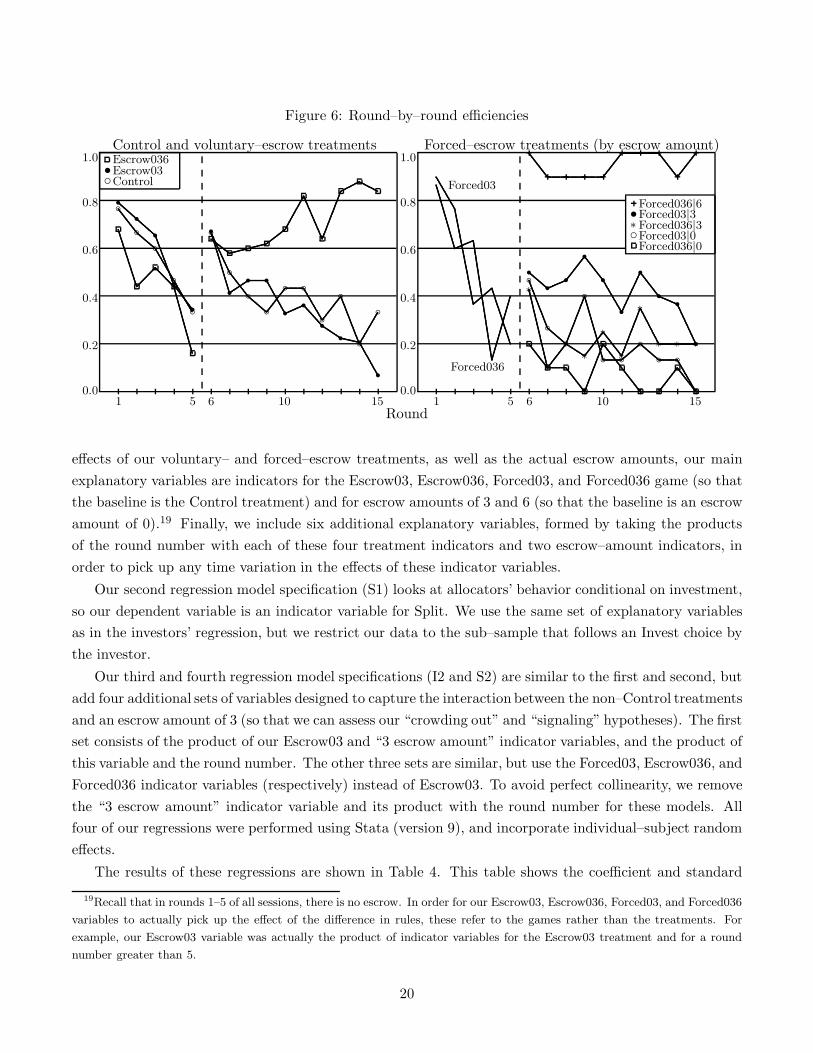
Figure 6: Round–by–round efficiencies

Control and voluntary–escrow treatments Forced–escrow treatments (by escrow amount)

Round

scEscrow036Escrow03Control

1 15 56 610 1015 150.0 0.0

0.2 0.2

0.4 0.4

0.6 0.6

0.8 0.8

1.0 1.0

b b bb

b

bb b b b b

b bb

b

r r rr r

rr r r

r r r r rr

pppppppppppppppppppppppppppppppppppppppppppppppppppppppppppppppppppppppppppppppppppppppppppppppppppppppppppppppppppppppppppppppppppppppppppppppppppppppppppppppppppppppppppppppppppppppppppppppppppppppppppppppppppppppppppppppppppppppppppppppppppppppppppppppppppppppppppppppppppppppppppppppppppppppppppppppppppppppppppppppppppppppppppppppppppppppppppppppppppppppppppppppppppppppppppppppppp

pppppppppppppppppppppppppppppppppppppppppppppppppppppppppppppppppppppppppppppppppppppppppppppppppppppppppppppppppppppppppppppppppppppppppppppppppppppppppppppppppppppppppppppppppppppppppppppppppppppppppppppppppppppppppppppppppppppppppppppppppppppppppppppppppppppppppppppppppppppppppppppppppppppppppppppppppppppppppppppppppppppppppppppppppppppppppppppppppppppppppppppppppppppppppppppppppppppppppppppppppppppppppppppppppppppppppppppppppppppppppppppppppppppppppppppppppppppppppppppppppppppppppppppppppppppppppppppppppppppppppppppppppppppppppppppppppppppppppppppppppppppppppppppppppppppppppppppppppppppppppppppppppppppppppppppppppppppppppppppppppppppppppppppppppppppppppppppppppppppppppppppppppppppppppppppppppppppppppppppppppppppppppppppppppppppppppppppppppppppppppppppppppppppppppppppppppppppppppppppppppppppppppppppppppppppppppppppppppppppppppppppppppppppppppppppppppppppppppppppppppppppppppppppppppppppppppppppp

pppppppppppppppppppppppppppppppppppppppppppppppppppppppppppppppppppppppppppppppppppppppppppppppppppppppppppppppppppppppppppppppppppppppppppppppppppppppppppppppppppppppppppppppppppppppppppppppppppppppppppppppppppppppppppppppppppppppppppppppppppppppppppppppppppppppppppppppppppppppppppppppppppppppppppppppppppppppppppppppppppppppppppppppppppppppppppppppppppppppppppppppppppppppppppppppppppppppppppppppp

ppppppppppppppppppppppppppppppppppppppppppppppppppppppppppppppppppppppppppppppppppppppppppppppppppppppppppppppppppppppppppppppppppppppppppppppppppppppppppppppppppppppppppppppppppppppppppppppppppppppppppppppppppppppppppppppppppppppppppppppppppppppppppppppppppppppppppppppppppppppppppppppppppppppppppppppppppppppppppppppppppppppppppppppppppppppppppppppppppppppppppppppppppppppppppppppppppppppppppppppppppppppppppppppppppppppppppppppppppppppppppppppppppppppppppppppppppppppppppppppppppppppppppppppppppppppppppppppppppppppppppppppppppppppppppppppppppppppppppppppppppppppppppppppppppppppppppppppppppppppppppppppppppppppppppppppppppppppppppppppppppppppppppppppppppppppppppppppppppppppppppppppppppppppppppppppppppppppppppppppppppppppppppppppppppppppppppppppppppppppppppppppppppppppppppppppppppppppppppppppppppppppppppppp

pppppppppppppppppppppppppppppppppppppppppppppppppppppppppppppppppppppppppppppppppppppppppppppppppppppppppppppppppppppppppppppppppppppppppppppppppppppppppppppppppppppppppppppppppppppppppppppppppppppppppppppppppppppppppppppppppppppppppppppppppppppppppppppppppppppppppppppppppppppppppppppppppppppppppppppppppppppppppppppppppppppppppppppppppppppppppppppppppppppppppppppppppppppppppppppppppppppppppppppppppppppppppppppppppppppppppppppppppppppppppppppppppppppppppppppppppppppppppppppppppppppppppppppppppppppppppppppppppppppppppppppppppppppppppppppppppppppp

pppppppppppppppppppppppppppppppppppppppppppppppppppppppppppppppppppppppppppppppppppppppppppppppppppppppppppppppppppppppppppppppppppppppppppppppppppppppppppppppppppppppppppppppppppppppppppppppppppppppppppppppppppppppppppppppppppppppppppppppppppppppppppppppppppppppppppppppppppppppppppppppppppppppppppppppppppppppppppppppppppppppppppppppppppppppppppppppppppp

pppppppppppppppppppppppppppppppppppppppppppppppppppppppppppppppppppppppppppppppppppppppppppppppppppppppppppppppppppppppppppppppppppppppppppppppppppppppppppppppppppppppppppppppppppppppppppppppppppppppppppppppppppppppppppppppppppppppppppppppppppppppppppppppppppppppppppppppppppppppppppppppppppppppppppppppppppppppppppppppppppppppppppppppppppppppppp

pppppppppppppppppppppppppppppppppppppppppppppppppppppppppppppppppppppppppppppppppppppp Forced03

Forced036

s*c

Forced036|6Forced03|3Forced036|3Forced03|0Forced036|0

pp

p pp

pppppppppppppppppppppppppppppppppppppppppppppppppppppppppppppppppppppppppppppppppppppppppppppppppppppppppppppppppppppppppppppppppppppppppppppppppppppppppppppppppppppppppppppppppppppppppppppppppppppppppppppppppppppppppppppppppppppppppppppppppppppppppppppppppppppppppppppppppppppppppppppppppppppppppppppppppppppppppppppppppppppppppppppppppppppppppppppppppppppppppppppppppppppppppppppppppppppppppppppppppppppppppppppppppppppppppppppppppppppppppppppppppppppppppppppppppppppppppppppppppppppppppppppppppppppppppppppppppppppppppppppppppppppppppppppppppppppppppppppppppppppppppppppppppppppppppppppppppppppppppppppppppppppppppppppppppppppppppppppppppppppppppppppp

pp p

pp

pppppppppppppppppppppppppppppppppppppppppppppppppppppppppppppppppppppppppppppppppppppppppppppppppppppppppppppppppppppppppppppppppppppppppppppppppppppppppppppppppppppppppppppppppppppppppppppppppppppppppppppppppppppppppppppppppppppppppppppppppppppppppppppppppppppppppppppppppppppppppppppppppppppppppppppppppppppppppppppppppppppppppppppppppppppppppppppppppppppppppppppppppppppppppppppppppppppppppppppppppppppppppppppppppppppppppppppppppppppppppppppppppppppppppppppppppppppppppppppppppppppppppppppppppppppppppppppppppppppppppppppppppppppppppppppppppppppppppppppppppppppppppppppppppppppppppppppppppppppppppppppppppppppppppppppppppppppppppppppppppppppppppppppppppppppppppppppppppppppppppppppppppppppppppppppppppppppppppppppppppppppppppppppppppppppppppppppppppppppppppppppppppppppppppppppppppppppppppppppppppppppppppppppppppppppppp b

b bb

b b b b bb

r r r r rr

r r rr

pppppppppppppppppppppppppppppppppppppppppppppppppppppppppppppppppppppppppppppppppppppppppppppppppppppppppppppppppppppppppppppppppppppppppppppppppppppppppppppppppppppppppppppppppppppppppppppppppppppppppppppppppppppppppppppppppppppppppppppppppppppppppppppppppppppppppppppppppppppppppppppppppppppppppppppppppppppppppppppppppppppppppppppppppppppppppppppppppppppppppppppppppppppppppppppppppppppppppppppppppppppppppppppppppppppppppppppppppppppppppppppppppppppppppppppppppppppppppppppppppppppppppppppppppppppppppppppppppppppppppppppppppppppppppppppppppppppppppppppppppppppppppppppppppppppppppppppppppppppppppppppppppppppppppppppppppppppppppppppppppppppppppppppppppppppppppppppppppppppppppppppppppppppppppppppppppppppppppppppppppppppppppppppppppppppppppppppppppppppppppppppppppppppppppppppppppppppppppppppppppppppppppppppppppppppppppppppppppppppppppppppppppppppppppppppppppppppppppppppppppppppppppppppppppppppppppppppppppppppppppppppppppppppppppppppppppppppp

ppppppppppppppppppppppppppppppppppppppppppppppppppppppppppppppppppppppppppppppppppppppppppppppppppppppppppppppppppppppppppppppppppppppppppppppppppppppppppppppppppppppppppppppppppppppppppppppppppppppppppppppppppppppppppppppppppppppppppppppppppppppppppppppppppppppppppppppppppppppppppppppppppppppppppppppppppppppppppppppppppppppppppppppppppppppppppppppppppppppppppppppppppppppppppppppppppppppppppppppppppppppppppppppppppppppppppppppppppppppppppppppppppppppppppppppppppppppppppppppppppppppppppppppppppppppppppppppppppp

pppppppppppppppppppppppppppppppppppppppppppppppppppppppppppppppppppppppppppppppppppppppppppppppppppppppppppppppppppppppppppppppppppppppppppppppppppppppppppppppppppppppppppppppppppppppppppppppppppppppppppppppppppppppppppppppppppppppppppppppppppppppppppppppppppppppppppppppppppppppppppppppppppppppppppppppppppppppppppppppppppppppppppppppppppppppppppppppppppppppppppppppppppppppppppppppppppppppppppppppppppppppppppppppppppppppppppppppppppppppppppppppppppppppppppppppppppppppppppppppppppppppppppppppppppppppppppppppppppppppppppppppppppppppppppppppppppppppppppppppppppppppppppppppppppppppppppppppppppppppppppppppppppppppppppppppppppppppppppppppppppppppppppppppppppppppppppppppppppppppppppppppppppppppppppppppppppppppppppppppppppppppppppppppppppppppppppppppppppppppppppppppppppppppppppppppppppppppppppppppppppppppppppppppppppppppppppppppppppppppppppppppppppppppppppppppppppppppppppppppppppppppppppppppppppppppppppppppppppppppppppppppppppppppppppppppppppppppppppppppppppppppppppppppppppppppppppppppppppppppppppppppppppppppppppppppppppppppppppppppppppppppppppppppppppppppppppppppppppppppppppppppppppppppppppppppppppppppppppppppppppppppppppppppppp

*

*

**

*

*

*

* * *

ppppppppppppppppppppppppppppppppppppppppppppppppppppppppppppppppppppppppppppppppppppppppppppppppppppppppppppppppppppppppppppppppppppppppppppppppppppppppppppppppppppppppppppppppppppppppppppppppppppppppppppppppppppppppppppppppppppppppppppppppppppppppppppppppppppppppppppppppppppppppppppppppppppppppppppppppppppppppppppppppppppppppppppppppppppppppppppppppppppppppppppppppppppppppppppppppppppppppppppppppppppppppppppppppppppppppppppppppppppppppppppppppppppppppppppppppppppppppppppppppppppppppppppppppppppppppppppppppppppppppppppppppppppppppppppppppppppppppppppppppppppppppppppppppppppppppppppppppppppppppppppppppppppppppppppppppppppppppppppppppppppppppppppppppppppppppppppp

pppppppppppppppppppppppppppppppppppppppppppppppppppppppppppppppppppppppppppppppppppppppppppppppppppppppppppppppppppppppppppppppppppppppppppppppppppppppppppppppppppppppppppppppppppppppppppppppppppppppppppppppppppppppppppppppppppppppppppppppppppppppppppppppppppppppppppppppppppppppppppppppppppppppppppp

pppppppppppppppppppppppppppppppppppppppppppppppppppppppppppppppppppppppppppppppppppppppppppppppppppppppppppppppppppppppppppppppppppppppppppppppppppppppppppppppppppppppppppppppppppppppppppppppppppppppppppppppppppppppppppppppppppppppppppppppppppppppppppppppppppppppppppppppppppppppppppppppppppppppppppppppppppppppppppppppppppppppppppppppppppppppppppppppppppppppppppppppppppppppppppppppppppppppppppppppppppppppppppppppppppppppppppppppppppppppppppppppppppppppppppppppppppppppppppppppppppppppppppppppppppppppppppppppppppppppppppppppppppppppppppppppppppppppppppppppppppppppppppppppppppppppppppppppppppppppppppppppppppppppppppppppppppppppppppppppppppp

effects of our voluntary– and forced–escrow treatments, as well as the actual escrow amounts, our mainexplanatory variables are indicators for the Escrow03, Escrow036, Forced03, and Forced036 game (so thatthe baseline is the Control treatment) and for escrow amounts of 3 and 6 (so that the baseline is an escrowamount of 0).19 Finally, we include six additional explanatory variables, formed by taking the productsof the round number with each of these four treatment indicators and two escrow–amount indicators, inorder to pick up any time variation in the effects of these indicator variables.

Our second regression model specification (S1) looks at allocators’ behavior conditional on investment,so our dependent variable is an indicator variable for Split. We use the same set of explanatory variablesas in the investors’ regression, but we restrict our data to the sub–sample that follows an Invest choice bythe investor.

Our third and fourth regression model specifications (I2 and S2) are similar to the first and second, butadd four additional sets of variables designed to capture the interaction between the non–Control treatmentsand an escrow amount of 3 (so that we can assess our “crowding out” and “signaling” hypotheses). The firstset consists of the product of our Escrow03 and “3 escrow amount” indicator variables, and the product ofthis variable and the round number. The other three sets are similar, but use the Forced03, Escrow036, andForced036 indicator variables (respectively) instead of Escrow03. To avoid perfect collinearity, we removethe “3 escrow amount” indicator variable and its product with the round number for these models. Allfour of our regressions were performed using Stata (version 9), and incorporate individual–subject randomeffects.

The results of these regressions are shown in Table 4. This table shows the coefficient and standard

19Recall that in rounds 1–5 of all sessions, there is no escrow. In order for our Escrow03, Escrow036, Forced03, and Forced036

variables to actually pick up the effect of the difference in rules, these refer to the games rather than the treatments. For

example, our Escrow03 variable was actually the product of indicator variables for the Escrow03 treatment and for a round

number greater than 5.

20

error for each variable in our four model specifications.20 Also shown, at the bottom of each column, isthe absolute value of the log–likelihood, as well as a pseudo–R2, for that model specification.21 Beforediscussing the results as they pertain to our hypotheses from Section 2.3, we briefly note some of the otherresults. First of all, neither pair of regression models nests or is nested by the other pair, so we cannot usestraightforward likelihood–ratio tests to compare them. However, we can use “information criteria” that,like likelihood–ratio tests, reward goodness–of–fit but punish free parameters. The Bayesian (also knownas Schwarz (1978)) Information Criterion favors the two simpler models: Model Specification I1 has anBIC of 2236.580, which is lower (and thus better) than the 2264.753 of Model Specification I2, and ModelSpecification S1’s BIC of 1119.422 is better than Model Specification S2’s BIC of 1153.793.22 The Akaike(1974) Information Criterion, which is more forgiving of free parameters than the BIC, favors the simplermodel for allocators but the less simple model for investors: Model Specification I2 has an AIC of 2145.518,which is lower (and thus better) than the 2151.412 of Model Specification I1, and Model Specification S1’sAIC of 1044.444 is better than Model Specification S2’s AIC of 1048.824. Because the simpler models tendto fare better under these information criteria, and because comparison of the columns of Table 4 suggeststhat the results are reasonably robust to the specification we use, we will generally confine our discussionof results to the first two columns—unless we need the extra variables used in the other columns.

For both investors and allocators, we find evidence of the usual restart effect: the coefficient of the“round ≥ 6” indicator variable is positive and significant. We also find evidence that behavior is time–dependent: for both player types, the coefficient for the round number is negative and significant. Thisnegative slope is consistent with the standard finding for trust games that investment and splitting decreaseover time. Our finding that allocators’ likelihood of choosing Split changes over time suggests that theirpreferences are evolving over time (or perhaps they are learning about their own preferences, or simply aredeveloping more understanding of the game); as there is no strategic uncertainty involved in this decision,it is hard to attribute these changes to learning about investor behavior. We note that other researchershave tested for, and found, changes in last–mover behavior over time in other games (see, for example,Cooper et al. (2003) in the ultimatum game).

The results in Table 4 also show differences in both Invest and Split frequencies across investmentamounts and across treatments. The two variables for a 6 escrow amount (that is, the “6 escrow amount”indicator and its product with the round number) are jointly significant for both investors and allocators(χ2 = 223.85, d.f. = 2, p < 0.001 for investors, χ2 = 72.89, d.f. = 2, p < 0.001 for allocators), as are thosefor a 3 escrow amount (χ2 = 116.06, d.f. = 2, p < 0.001 for investors, χ2 = 18.25, d.f. = 2, p ≈ 0.001 forallocators). For investors, the four sets of treatment variables (Escrow03 and Escrow03*round, and so on)are each jointly significantly different from zero (with significance test results ranging from χ2 = 16.56,d.f. = 2, p < 0.001 to χ2 = 52.10, d.f. = 2, p < 0.001), but this is not always true for allocators (rangingfrom χ2 = 3.58, d.f. = 2, p ≈ 0.167 to χ2 = 14.83, d.f. = 2, p < 0.001).

However, these joint significance tests are unsatisfactory for two reasons. First, the sets of variables

20Note that Model Specification S2 leads to some very large standard errors.21The pseudo–R2 values we report were computed by rescaling the log–likelihoods into [0,1], such that a model with no

right–hand–side variables other than the constant term maps to zero, and a perfect fit maps to one.22The BIC is equivalent to Klein and Brown (1984)’s “minimum–prior–information” posterior–odds criterion.

21

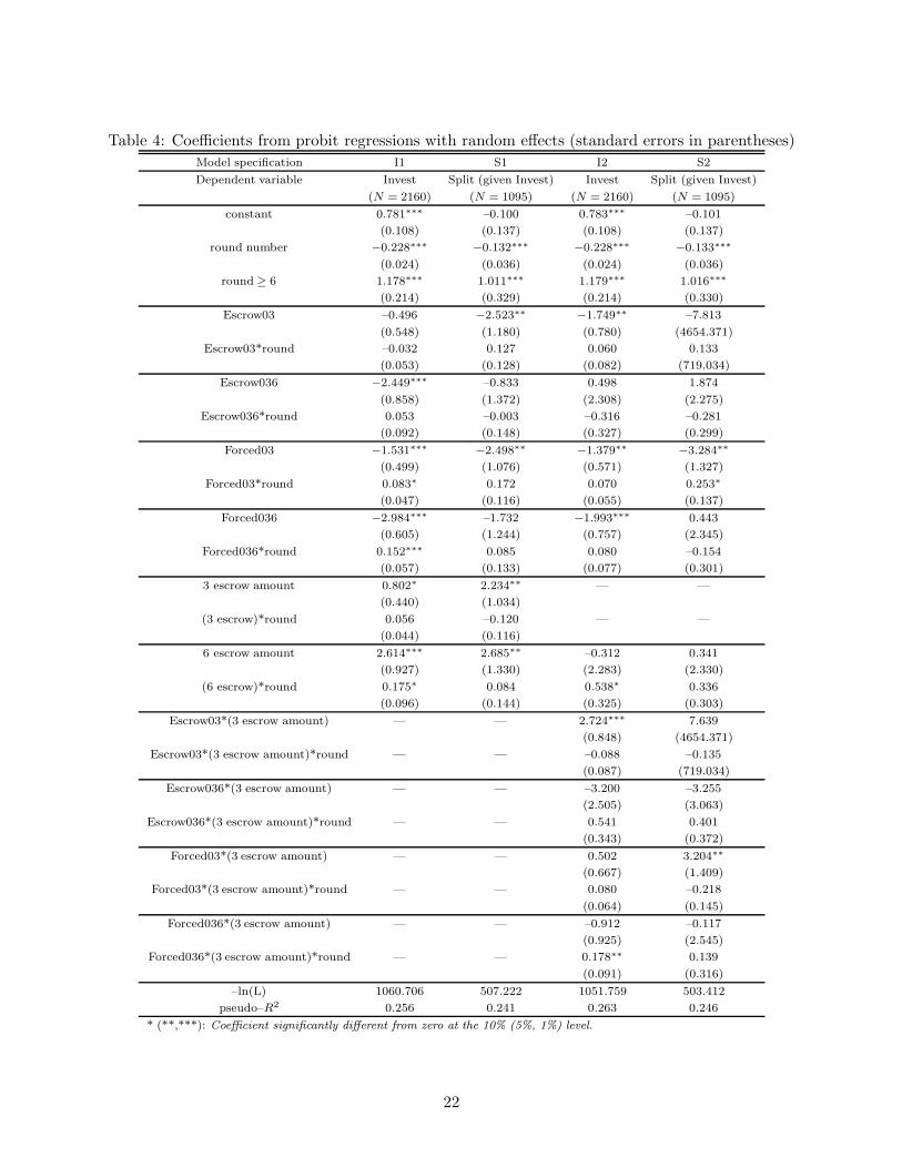
Table 4: Coefficients from probit regressions with random effects (standard errors in parentheses)Model specification I1 S1 I2 S2

Dependent variable Invest Split (given Invest) Invest Split (given Invest)

(N = 2160) (N = 1095) (N = 2160) (N = 1095)

constant 0.781∗∗∗ –0.100 0.783∗∗∗ –0.101

(0.108) (0.137) (0.108) (0.137)

round number −0.228∗∗∗ −0.132∗∗∗ −0.228∗∗∗ −0.133∗∗∗

(0.024) (0.036) (0.024) (0.036)

round ≥ 6 1.178∗∗∗ 1.011∗∗∗ 1.179∗∗∗ 1.016∗∗∗

(0.214) (0.329) (0.214) (0.330)

Escrow03 –0.496 −2.523∗∗ −1.749∗∗ –7.813

(0.548) (1.180) (0.780) (4654.371)

Escrow03*round –0.032 0.127 0.060 0.133

(0.053) (0.128) (0.082) (719.034)

Escrow036 −2.449∗∗∗ –0.833 0.498 1.874

(0.858) (1.372) (2.308) (2.275)

Escrow036*round 0.053 –0.003 –0.316 –0.281

(0.092) (0.148) (0.327) (0.299)

Forced03 −1.531∗∗∗ −2.498∗∗ −1.379∗∗ −3.284∗∗

(0.499) (1.076) (0.571) (1.327)

Forced03*round 0.083∗ 0.172 0.070 0.253∗

(0.047) (0.116) (0.055) (0.137)

Forced036 −2.984∗∗∗ –1.732 −1.993∗∗∗ 0.443

(0.605) (1.244) (0.757) (2.345)

Forced036*round 0.152∗∗∗ 0.085 0.080 –0.154

(0.057) (0.133) (0.077) (0.301)

3 escrow amount 0.802∗ 2.234∗∗ — —

(0.440) (1.034)

(3 escrow)*round 0.056 –0.120 — —

(0.044) (0.116)

6 escrow amount 2.614∗∗∗ 2.685∗∗ –0.312 0.341

(0.927) (1.330) (2.283) (2.330)

(6 escrow)*round 0.175∗ 0.084 0.538∗ 0.336

(0.096) (0.144) (0.325) (0.303)

Escrow03*(3 escrow amount) — — 2.724∗∗∗ 7.639

(0.848) (4654.371)

Escrow03*(3 escrow amount)*round — — –0.088 –0.135

(0.087) (719.034)

Escrow036*(3 escrow amount) — — –3.200 –3.255

(2.505) (3.063)

Escrow036*(3 escrow amount)*round — — 0.541 0.401

(0.343) (0.372)

Forced03*(3 escrow amount) — — 0.502 3.204∗∗

(0.667) (1.409)

Forced03*(3 escrow amount)*round — — 0.080 –0.218

(0.064) (0.145)

Forced036*(3 escrow amount) — — –0.912 –0.117

(0.925) (2.545)

Forced036*(3 escrow amount)*round — — 0.178∗∗ 0.139

(0.091) (0.316)

–ln(L) 1060.706 507.222 1051.759 503.412

pseudo–R2 0.256 0.241 0.263 0.246

* (**,***): Coefficient significantly different from zero at the 10% (5%, 1%) level.

22

we are interested in contain interaction terms, and it is well known that when nonlinear regression models(such as probits) are used, the marginal effect of the interaction between two variables is not equal to thecoefficient of the interaction term. (See Ai and Norton (2003) and Norton, Wang, and Ai (2004).) Second,even if we know that a particular set of variables is jointly significant, this alone does not tell us what theactual effect of these variables is; for example, we have seen that the “6 escrow amount” indicator and itsproduct with the round number are jointly significant for both investors and allocators, but we do not yetknow whether Invest and/or Split choices are more likely after a 6 escrow amount than after a 0 escrowamount. The total effect in round t of a 6 escrow amount, rather than a 0 escrow amount, on the argumentof the normal c.d.f. used in the probit model is given by the expression β6 escrow amount +β(6 escrow)*round ·t(where βY is the coefficient of the variable Y ). So, the incremental effect (the analogue to a marginal effect,for a discrete variable) of a 6 escrow amount rather than a 0 escrow amount in round t has the form

Φ(X · B + β6 escrow amount + β(6 escrow)*round · t

)− Φ

(X · B

)

where X is the row vector of the other right–hand variables’ values, and B is the column vector of theircoefficient estimates. This effect will depend on which values we specify for the other right–hand variables;in the following, we will use either the unconditional sample mean or, in some cases, the mean conditionalon an appropriate sub–sample.

Figure 7 shows, for each round and for both investors and allocators, the estimated value of theexpression above (left panel), as well as corresponding expressions for the effect of a 6 escrow amountversus a 3 escrow amount (center panel), and that of a 3 escrow amount versus a 0 escrow amount (rightpanel), all based on Model Specifications I1 and S1 (that is, the coefficients shown in the first two columns ofTable 4). The figure shows not only the point estimates of these effects, but also estimated 95% confidenceintervals.23

As the left and center panels of the figure show, not only are the point estimates for the effect of a 6escrow amount versus either a 0 or a 3 escrow amount always positive for both investors and allocators, butthe corresponding confidence intervals are as well. This means that both Invest and Split are significantlymore likely (at the 5% level) after a 6 escrow amount than after a lower one—consistent with our Hypotheses1 and 2, which predicted exactly this. Moreover, the point estimates of these effects grow monotonicallyover the length of the session, implying that differences between play following a 6 escrow amount and thatfollowing either a 0 or a 3 escrow amount become stronger as subjects gain experience.

The right panel shows that initially, both Invest and Split are significantly more likely after a 3 escrowamount than after a 0 escrow amount. However, the point estimate of this effect decreases over time forboth player types. It remains significant in all rounds for investors, but by the end of the session becomesinsignificant for allocators. To the extent that this effect is significant (for either investors or allocators),it is at odds with our Hypotheses 3 and 4, according to which frequencies of Invest and Split should be thesame following either a 3 or a 0 escrow amount.

23In this figure and others, we put results for investors and allocators in the same panel for reasons of space; we are at

no time statistically testing any effect on investor behavior versus the corresponding effect on allocator behavior. Also, we

truncate confidence intervals at +1 and –1.

23

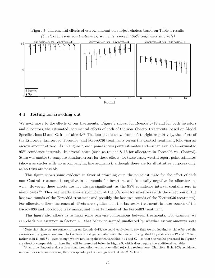
Figure 7: Incremental effects of escrow amount on subject choices based on Table 4 results(Circles represent point estimates; segments represent 95% confidence intervals)

rb InvestSplit

+1

0

–16 6 69 9 912 12 1215 15 15

escrow=6 vs. escrow=0 escrow=6 vs. escrow=3 escrow=3 vs. escrow=0

Round

b b b b b b b b b br r r r r r r r r rb b b b b b b b b br r r r r r r r r r

b b b b b b b b b br r r r r r r r r r

4.4 Testing for crowding out

We next move to the effects of our treatments. Figure 8 shows, for Rounds 6–15 and for both investorsand allocators, the estimated incremental effects of each of the non–Control treatments, based on ModelSpecifications I2 and S2 from Table 4.24 The four panels show, from left to right respectively, the effects ofthe Escrow03, Escrow036, Forced03, and Forced036 treatments versus the Control treatment, following anescrow amount of zero. As in Figure 7, each panel shows point estimates and—when available—estimated95% confidence intervals. In several cases (such as rounds 8–15 for allocators in Forced03 vs. Control),Stata was unable to compute standard errors for these effects; for these cases, we still report point estimates(shown as circles with no accompanying line segments), although these are for illustrative purposes only,as no tests are possible.

This figure shows some evidence in favor of crowding out: the point estimate for the effect of eachnon–Control treatment is negative in all rounds for investors, and is usually negative for allocators aswell. However, these effects are not always significant, as the 95% confidence interval contains zero inmany cases.25 They are nearly always significant at the 5% level for investors (with the exception of thelast two rounds of the Forced03 treatment and possibly the last two rounds of the Escrow036 treatment).For allocators, these incremental effects are significant in the Escrow03 treatment, in later rounds of theEscrow036 and Forced036 treatments, and in early rounds of the Forced03 treatment.

This figure also allows us to make some pairwise comparisons between treatments. For example, wecan check our assertion in Section 4.1 that behavior seemed unaffected by whether escrow amounts were

24Note that since we are concentrating on Rounds 6–15, we could equivalently say that we are looking at the effects of the

various escrow games compared to the basic trust game. Also note that we are using Model Specifications I2 and S2 here

rather than I1 and S1—even though we are not using the extra variables in I2 and S2—so that the results presented in Figure 8

are directly comparable to those that will be presented below in Figure 9, which does require the additional variables.25Since crowding out makes a directional prediction, we use one–tailed rejection regions here. Therefore, if the 95% confidence

interval does not contain zero, the corresponding effect is significant at the 2.5% level.

24

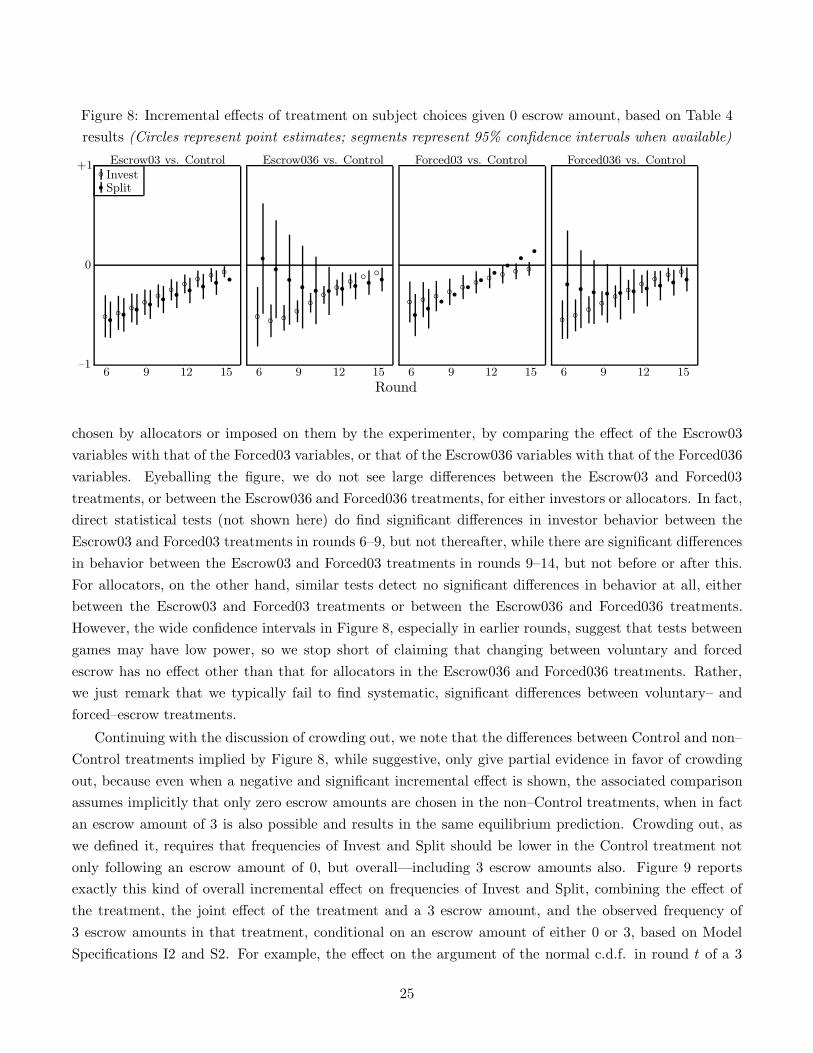
Figure 8: Incremental effects of treatment on subject choices given 0 escrow amount, based on Table 4results (Circles represent point estimates; segments represent 95% confidence intervals when available)

rb InvestSplit

+1

0

–16 6 6 69 9 9 912 12 12 1215 15 15 15

Escrow03 vs. Control Escrow036 vs. Control Forced03 vs. Control Forced036 vs. Control

Round

b b b b b b b b b br r r r r r r r r r

b b b b b b b b b br r r r r r r r r r b b b b b b b b b br r r r r r r r r r

b b b b b b b b b br r r r r r r r r r

chosen by allocators or imposed on them by the experimenter, by comparing the effect of the Escrow03variables with that of the Forced03 variables, or that of the Escrow036 variables with that of the Forced036variables. Eyeballing the figure, we do not see large differences between the Escrow03 and Forced03treatments, or between the Escrow036 and Forced036 treatments, for either investors or allocators. In fact,direct statistical tests (not shown here) do find significant differences in investor behavior between theEscrow03 and Forced03 treatments in rounds 6–9, but not thereafter, while there are significant differencesin behavior between the Escrow03 and Forced03 treatments in rounds 9–14, but not before or after this.For allocators, on the other hand, similar tests detect no significant differences in behavior at all, eitherbetween the Escrow03 and Forced03 treatments or between the Escrow036 and Forced036 treatments.However, the wide confidence intervals in Figure 8, especially in earlier rounds, suggest that tests betweengames may have low power, so we stop short of claiming that changing between voluntary and forcedescrow has no effect other than that for allocators in the Escrow036 and Forced036 treatments. Rather,we just remark that we typically fail to find systematic, significant differences between voluntary– andforced–escrow treatments.

Continuing with the discussion of crowding out, we note that the differences between Control and non–Control treatments implied by Figure 8, while suggestive, only give partial evidence in favor of crowdingout, because even when a negative and significant incremental effect is shown, the associated comparisonassumes implicitly that only zero escrow amounts are chosen in the non–Control treatments, when in factan escrow amount of 3 is also possible and results in the same equilibrium prediction. Crowding out, aswe defined it, requires that frequencies of Invest and Split should be lower in the Control treatment notonly following an escrow amount of 0, but overall—including 3 escrow amounts also. Figure 9 reportsexactly this kind of overall incremental effect on frequencies of Invest and Split, combining the effect ofthe treatment, the joint effect of the treatment and a 3 escrow amount, and the observed frequency of3 escrow amounts in that treatment, conditional on an escrow amount of either 0 or 3, based on ModelSpecifications I2 and S2. For example, the effect on the argument of the normal c.d.f. in round t of a 3

25

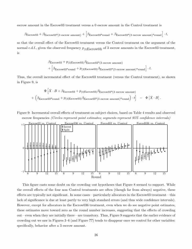
escrow amount in the Escrow03 treatment versus a 0 escrow amount in the Control treatment is

βEscrow03 + βEscrow03*(3 escrow amount) +[βEscrow03*round + βEscrow03*(3 escrow amount)*round

]· t,

so that the overall effect of the Escrow03 treatment versus the Control treatment on the argument of thenormal c.d.f., given the observed frequency p(3|Escrow03) of 3 escrow amounts in the Escrow03 treatment,is

βEscrow03 + p(3|Escrow03)βEscrow03*(3 escrow amount)

+[βEscrow03*round + p(3|Escrow03)βEscrow03*(3 escrow amount)*round

]· t.

Thus, the overall incremental effect of the Escrow03 treatment (versus the Control treatment), as shownin Figure 9, is

Φ[X · B + βEscrow03 + p(3|Escrow03)βEscrow03*(3 escrow amount)

+(βEscrow03*round + p(3|Escrow03)βEscrow03*(3 escrow amount)*round

)· t

]− Φ

[X · B

].

Figure 9: Incremental overall effects of treatment on subject choices, based on Table 4 results and observedescrow frequencies (Circles represent point estimates; segments represent 95% confidence intervals)

rbInvestSplit

+1

0

–16 6 6 69 9 9 912 12 12 1215 15 15 15

Escrow03 vs. Control Escrow036 vs. Control Forced03 vs. Control Forced036 vs. Control

Round

b b b b b b b b b br r r r r r r r r r

b b b b b b b b b br r r r r r r r r r b b b b b b b b b br r r r r r r r r r

b b b b b b b b b br r r r r r r r r r

This figure casts some doubt on the crowding–out hypotheses that Figure 8 seemed to support. Whilethe overall effects of the four non–Control treatments are often (though far from always) negative, theseeffects are typically not significant. In some cases—particularly allocators in the Escrow03 treatment—thislack of significance is due at least partly to very high standard errors (and thus wide confidence intervals).However, except for allocators in the Escrow036 treatment, even when we do see negative point estimates,these estimates move toward zero as the round number increases, suggesting that the effects of crowdingout—even when they are initially there—are transitory. Thus, Figure 9 suggests that the earlier evidence ofcrowding out we saw in Figures 3–6 (and Figure ??) tends to disappear once we control for other variables:specifically, behavior after a 3 escrow amount.

26

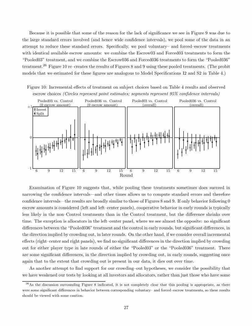
Because it is possible that some of the reason for the lack of significance we see in Figure 9 was due tothe large standard errors involved (and hence wide confidence intervals), we pool some of the data in anattempt to reduce these standard errors. Specifically, we pool voluntary– and forced–escrow treatmentswith identical available escrow amounts: we combine the Escrow03 and Forced03 treatments to form the“Pooled03” treatment, and we combine the Escrow036 and Forced036 treatments to form the “Pooled036”treatment.26 Figure 10 re–creates the results of Figures 8 and 9 using these pooled treatments. (The probitmodels that we estimated for these figures are analogous to Model Specifications I2 and S2 in Table 4.)

Figure 10: Incremental effects of treatment on subject choices based on Table 4 results and observedescrow choices (Circles represent point estimates; segments represent 95% confidence intervals)

rb InvestSplit

+1

0

–16 6 6 69 9 9 912 12 12 1215 15 15 15

Pooled03 vs. Control Pooled036 vs. Control Pooled03 vs. Control Pooled036 vs. Control(0 escrow amount) (0 escrow amount) (overall) (overall)

Round

b b b b b b b b b br r r r r r r r r r

b b b b b b b b b br r r r r r r r r r b b b b b b b b b br r r r r r r r r r

b b b b b b b b b br r r r r r r r r r

Examination of Figure 10 suggests that, while pooling these treatments sometimes does succeed innarrowing the confidence intervals—and other times allows us to compute standard errors and thereforeconfidence intervals—the results are broadly similar to those of Figures 8 and 9. If only behavior following 0escrow amounts is considered (left and left–center panels), cooperative behavior in early rounds is typicallyless likely in the non–Control treatments than in the Control treatment, but the difference shrinks overtime. The exception is allocators in the left–center panel, where we see almost the opposite: no significantdifferences between the “Pooled036” treatment and the control in early rounds, but significant differences, inthe direction implied by crowding out, in later rounds. On the other hand, if we consider overall incrementaleffects (right–center and right panels), we find no significant differences in the direction implied by crowdingout for either player type in late rounds of either the “Pooled03” or the “Pooled036” treatment. Thereare some significant differences, in the direction implied by crowding out, in early rounds, suggesting onceagain that to the extent that crowding out is present in our data, it dies out over time.

As another attempt to find support for our crowding–out hypotheses, we consider the possibility thatwe have weakened our tests by looking at all investors and allocators, rather than just those who have some

26As the discussion surrounding Figure 8 indicated, it is not completely clear that this pooling is appropriate, as there

were some significant differences in behavior between corresponding voluntary– and forced–escrow treatments, so these results

should be viewed with some caution.

27

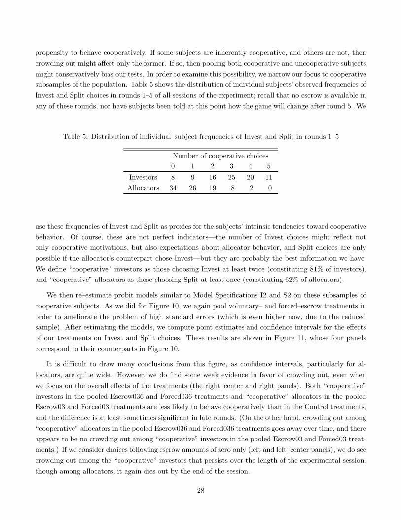
propensity to behave cooperatively. If some subjects are inherently cooperative, and others are not, thencrowding out might affect only the former. If so, then pooling both cooperative and uncooperative subjectsmight conservatively bias our tests. In order to examine this possibility, we narrow our focus to cooperativesubsamples of the population. Table 5 shows the distribution of individual subjects’ observed frequencies ofInvest and Split choices in rounds 1–5 of all sessions of the experiment; recall that no escrow is available inany of these rounds, nor have subjects been told at this point how the game will change after round 5. We

Table 5: Distribution of individual–subject frequencies of Invest and Split in rounds 1–5

Number of cooperative choices0 1 2 3 4 5

Investors 8 9 16 25 20 11Allocators 34 26 19 8 2 0

use these frequencies of Invest and Split as proxies for the subjects’ intrinsic tendencies toward cooperativebehavior. Of course, these are not perfect indicators—the number of Invest choices might reflect notonly cooperative motivations, but also expectations about allocator behavior, and Split choices are onlypossible if the allocator’s counterpart chose Invest—but they are probably the best information we have.We define “cooperative” investors as those choosing Invest at least twice (constituting 81% of investors),and “cooperative” allocators as those choosing Split at least once (constituting 62% of allocators).

We then re–estimate probit models similar to Model Specifications I2 and S2 on these subsamples ofcooperative subjects. As we did for Figure 10, we again pool voluntary– and forced–escrow treatments inorder to ameliorate the problem of high standard errors (which is even higher now, due to the reducedsample). After estimating the models, we compute point estimates and confidence intervals for the effectsof our treatments on Invest and Split choices. These results are shown in Figure 11, whose four panelscorrespond to their counterparts in Figure 10.

It is difficult to draw many conclusions from this figure, as confidence intervals, particularly for al-locators, are quite wide. However, we do find some weak evidence in favor of crowding out, even whenwe focus on the overall effects of the treatments (the right–center and right panels). Both “cooperative”investors in the pooled Escrow036 and Forced036 treatments and “cooperative” allocators in the pooledEscrow03 and Forced03 treatments are less likely to behave cooperatively than in the Control treatments,and the difference is at least sometimes significant in late rounds. (On the other hand, crowding out among“cooperative” allocators in the pooled Escrow036 and Forced036 treatments goes away over time, and thereappears to be no crowding out among “cooperative” investors in the pooled Escrow03 and Forced03 treat-ments.) If we consider choices following escrow amounts of zero only (left and left–center panels), we do seecrowding out among the “cooperative” investors that persists over the length of the experimental session,though among allocators, it again dies out by the end of the session.

28

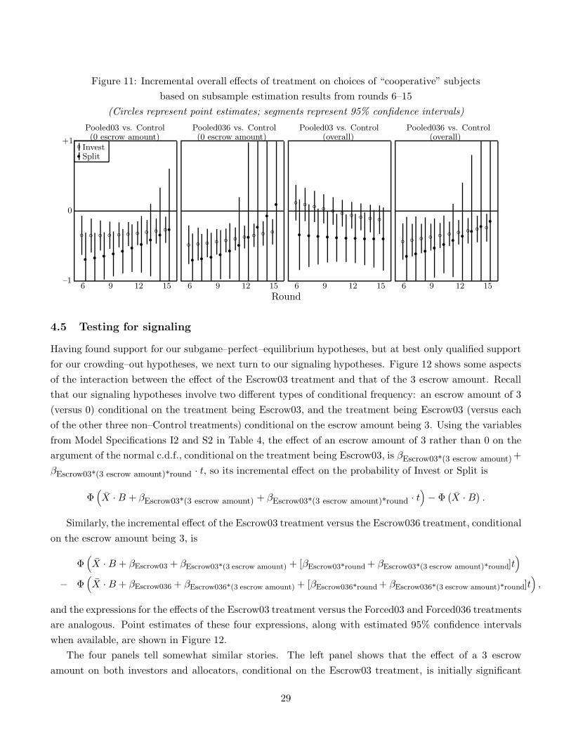
Figure 11: Incremental overall effects of treatment on choices of “cooperative” subjectsbased on subsample estimation results from rounds 6–15

(Circles represent point estimates; segments represent 95% confidence intervals)

rb InvestSplit

+1

0

–16 6 6 69 9 9 912 12 12 1215 15 15 15

Pooled03 vs. Control Pooled036 vs. Control Pooled03 vs. Control Pooled036 vs. Control(0 escrow amount) (0 escrow amount) (overall) (overall)

Round

b b b b b b b b b br r r r r r r r r r b b b b b b b b b b

r r r r r r r r r r b b b b b b b b b br r r r r r r r r r b b b b b b b b b br r r r r r r r r r

4.5 Testing for signaling

Having found support for our subgame–perfect–equilibrium hypotheses, but at best only qualified supportfor our crowding–out hypotheses, we next turn to our signaling hypotheses. Figure 12 shows some aspectsof the interaction between the effect of the Escrow03 treatment and that of the 3 escrow amount. Recallthat our signaling hypotheses involve two different types of conditional frequency: an escrow amount of 3(versus 0) conditional on the treatment being Escrow03, and the treatment being Escrow03 (versus eachof the other three non–Control treatments) conditional on the escrow amount being 3. Using the variablesfrom Model Specifications I2 and S2 in Table 4, the effect of an escrow amount of 3 rather than 0 on theargument of the normal c.d.f., conditional on the treatment being Escrow03, is βEscrow03*(3 escrow amount)+βEscrow03*(3 escrow amount)*round · t, so its incremental effect on the probability of Invest or Split is

Φ(X · B + βEscrow03*(3 escrow amount) + βEscrow03*(3 escrow amount)*round · t

)− Φ

(X · B

).

Similarly, the incremental effect of the Escrow03 treatment versus the Escrow036 treatment, conditionalon the escrow amount being 3, is

Φ(X · B + βEscrow03 + βEscrow03*(3 escrow amount) + [βEscrow03*round + βEscrow03*(3 escrow amount)*round]t

)

− Φ(X · B + βEscrow036 + βEscrow036*(3 escrow amount) + [βEscrow036*round + βEscrow036*(3 escrow amount)*round]t

),

and the expressions for the effects of the Escrow03 treatment versus the Forced03 and Forced036 treatmentsare analogous. Point estimates of these four expressions, along with estimated 95% confidence intervalswhen available, are shown in Figure 12.

The four panels tell somewhat similar stories. The left panel shows that the effect of a 3 escrowamount on both investors and allocators, conditional on the Escrow03 treatment, is initially significant

29

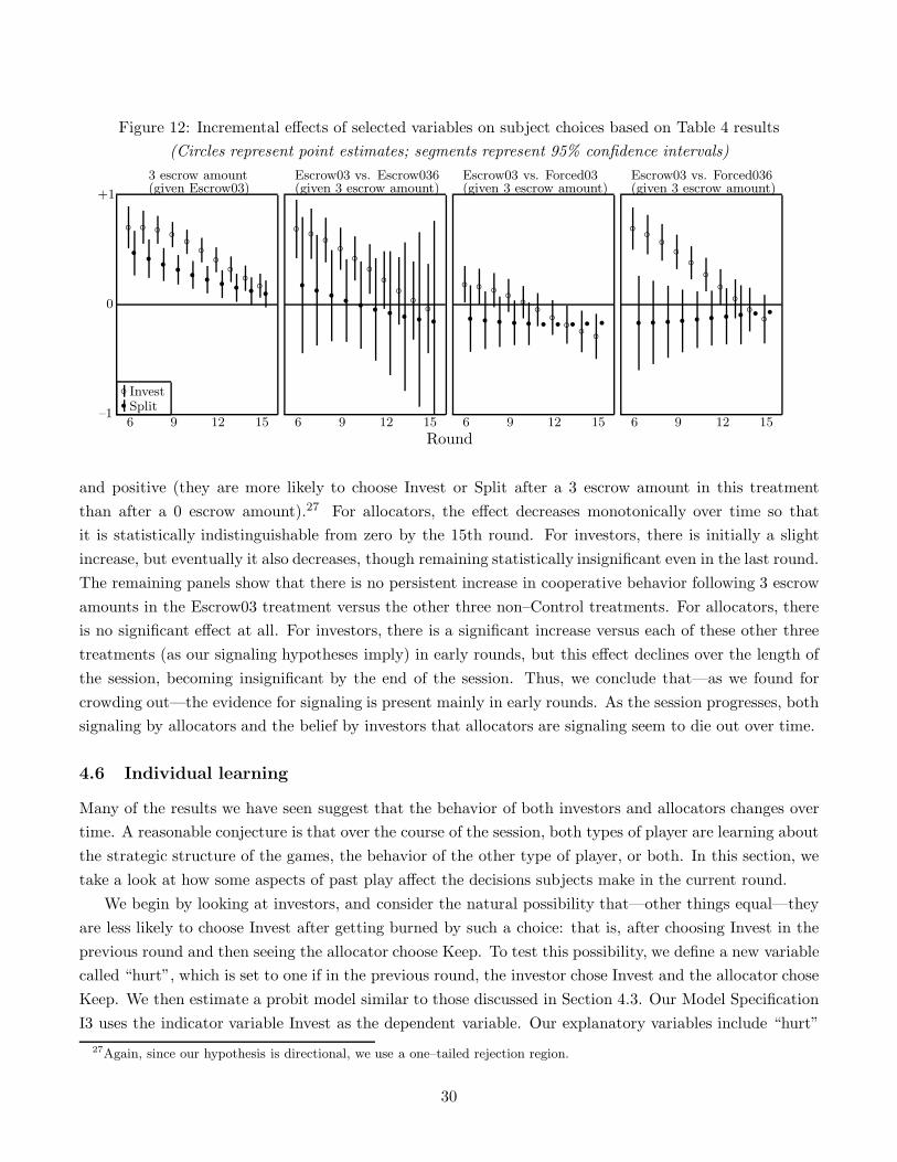
Figure 12: Incremental effects of selected variables on subject choices based on Table 4 results(Circles represent point estimates; segments represent 95% confidence intervals)

rb InvestSplit

+1

0

–16 6 6 69 9 9 912 12 12 1215 15 15 15

3 escrow amount(given Escrow03)

Escrow03 vs. Escrow036(given 3 escrow amount)

Escrow03 vs. Forced03(given 3 escrow amount)

Escrow03 vs. Forced036(given 3 escrow amount)

Round

b b b b b b b b b br r r r r r r r r r

b b b b b b b b b br r r r r r r r r rb b b b b b b b b br r r r r r r r r r

b b b b b b b b b br r r r r r r r r r

and positive (they are more likely to choose Invest or Split after a 3 escrow amount in this treatmentthan after a 0 escrow amount).27 For allocators, the effect decreases monotonically over time so thatit is statistically indistinguishable from zero by the 15th round. For investors, there is initially a slightincrease, but eventually it also decreases, though remaining statistically insignificant even in the last round.The remaining panels show that there is no persistent increase in cooperative behavior following 3 escrowamounts in the Escrow03 treatment versus the other three non–Control treatments. For allocators, thereis no significant effect at all. For investors, there is a significant increase versus each of these other threetreatments (as our signaling hypotheses imply) in early rounds, but this effect declines over the length ofthe session, becoming insignificant by the end of the session. Thus, we conclude that—as we found forcrowding out—the evidence for signaling is present mainly in early rounds. As the session progresses, bothsignaling by allocators and the belief by investors that allocators are signaling seem to die out over time.

4.6 Individual learning

Many of the results we have seen suggest that the behavior of both investors and allocators changes overtime. A reasonable conjecture is that over the course of the session, both types of player are learning aboutthe strategic structure of the games, the behavior of the other type of player, or both. In this section, wetake a look at how some aspects of past play affect the decisions subjects make in the current round.

We begin by looking at investors, and consider the natural possibility that—other things equal—theyare less likely to choose Invest after getting burned by such a choice: that is, after choosing Invest in theprevious round and then seeing the allocator choose Keep. To test this possibility, we define a new variablecalled “hurt”, which is set to one if in the previous round, the investor chose Invest and the allocator choseKeep. We then estimate a probit model similar to those discussed in Section 4.3. Our Model SpecificationI3 uses the indicator variable Invest as the dependent variable. Our explanatory variables include “hurt”

27Again, since our hypothesis is directional, we use a one–tailed rejection region.

30

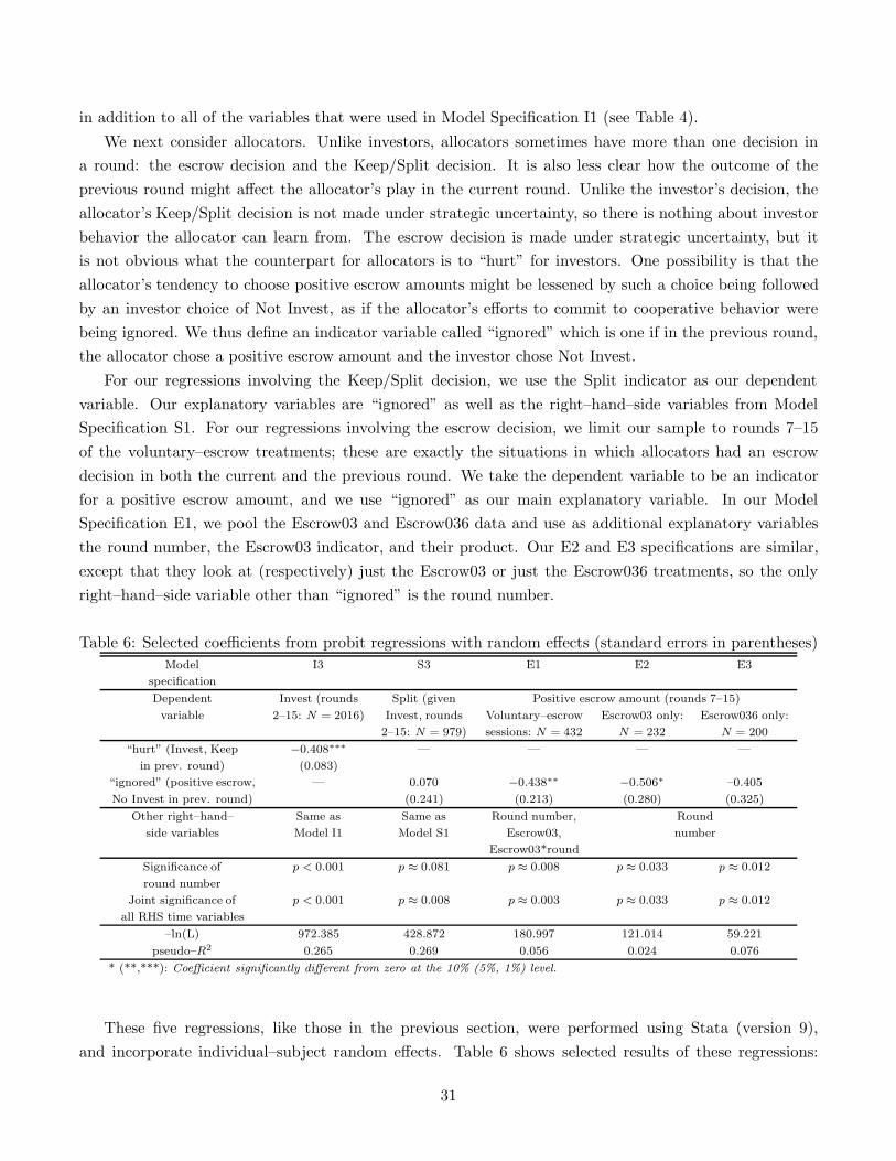
in addition to all of the variables that were used in Model Specification I1 (see Table 4).We next consider allocators. Unlike investors, allocators sometimes have more than one decision in

a round: the escrow decision and the Keep/Split decision. It is also less clear how the outcome of theprevious round might affect the allocator’s play in the current round. Unlike the investor’s decision, theallocator’s Keep/Split decision is not made under strategic uncertainty, so there is nothing about investorbehavior the allocator can learn from. The escrow decision is made under strategic uncertainty, but itis not obvious what the counterpart for allocators is to “hurt” for investors. One possibility is that theallocator’s tendency to choose positive escrow amounts might be lessened by such a choice being followedby an investor choice of Not Invest, as if the allocator’s efforts to commit to cooperative behavior werebeing ignored. We thus define an indicator variable called “ignored” which is one if in the previous round,the allocator chose a positive escrow amount and the investor chose Not Invest.

For our regressions involving the Keep/Split decision, we use the Split indicator as our dependentvariable. Our explanatory variables are “ignored” as well as the right–hand–side variables from ModelSpecification S1. For our regressions involving the escrow decision, we limit our sample to rounds 7–15of the voluntary–escrow treatments; these are exactly the situations in which allocators had an escrowdecision in both the current and the previous round. We take the dependent variable to be an indicatorfor a positive escrow amount, and we use “ignored” as our main explanatory variable. In our ModelSpecification E1, we pool the Escrow03 and Escrow036 data and use as additional explanatory variablesthe round number, the Escrow03 indicator, and their product. Our E2 and E3 specifications are similar,except that they look at (respectively) just the Escrow03 or just the Escrow036 treatments, so the onlyright–hand–side variable other than “ignored” is the round number.

Table 6: Selected coefficients from probit regressions with random effects (standard errors in parentheses)Model I3 S3 E1 E2 E3

specification

Dependent Invest (rounds Split (given Positive escrow amount (rounds 7–15)

variable 2–15: N = 2016) Invest, rounds Voluntary–escrow Escrow03 only: Escrow036 only:

2–15: N = 979) sessions: N = 432 N = 232 N = 200

“hurt” (Invest, Keep −0.408∗∗∗ — — — —

in prev. round) (0.083)

“ignored” (positive escrow, — 0.070 −0.438∗∗ −0.506∗ –0.405

No Invest in prev. round) (0.241) (0.213) (0.280) (0.325)

Other right–hand– Same as Same as Round number, Round

side variables Model I1 Model S1 Escrow03, number

Escrow03*round

Significance of p < 0.001 p ≈ 0.081 p ≈ 0.008 p ≈ 0.033 p ≈ 0.012

round number

Joint significance of p < 0.001 p ≈ 0.008 p ≈ 0.003 p ≈ 0.033 p ≈ 0.012

all RHS time variables

–ln(L) 972.385 428.872 180.997 121.014 59.221

pseudo–R2 0.265 0.269 0.056 0.024 0.076

* (**,***): Coefficient significantly different from zero at the 10% (5%, 1%) level.

These five regressions, like those in the previous section, were performed using Stata (version 9),and incorporate individual–subject random effects. Table 6 shows selected results of these regressions:

31

coefficients and standard errors for our new variables, as well as the log–likelihood and the pseudo–R2 foreach model specification. Also shown are the p–values from significance tests for the round number andfrom χ2 tests of joint significance for all right–hand–side time variables—the round number as well as itsproducts with the various treatment and escrow–amount indicators—for each model specification.

The results in this table indicate that, in decisions involving strategic uncertainty (investment andescrow, but not Split/Keep), subjects are learning from the feedback they receive about the other playertype, and in particular, the information present in our “hurt” and “ignored” variables. Investors aresignificantly less likely to choose Invest in the next round if they chose Invest in the current round, and theallocator’s response was Keep. Based on the pooled Escrow03 and Escrow036 data, we see that allocators,for their part, are significantly less likely to choose a positive escrow amount in the next round if they didso in the current round, but the investor chose Not Invest, though this association becomes less significant,or even insignificant, if we look at the Escrow03 and Escrow036 data separately. Perhaps not surprisingly,we do not see any significant relationship between the “ignored” variable and the likelihood of allocators’choosing Split; as mentioned before, the Keep/Split decision is not made under any strategic uncertainty,so it’s difficult to imagine allocators’ learning anything about investors that would be useful in makingthis decision. We also see that in all five columns, the collection of all right–hand–side time variables aresignificant (at least at the 5% level), as is the round number itself (at least at the 10% level), suggestingthat these “hurt” and “ignored” variables do not fully capture the learning investors are doing. It couldbe that investors and allocators are also learning via information other than that present in these variables(possibly including results from rounds other than the most recent), or they might be learning partlythrough their own introspection between rounds, or both.

5 Conclusions

There is a growing literature studying mechanisms designed to induce cooperative behavior—and henceraise efficiency—in situations where rational, self–interested behavior is predicted to lead to inefficientoutcomes. The trust game is a simple example of such a situation: the moral–hazard problem for allocatorsleads investors (in theory) to avoid investment, even though investment always leads to gains. We look atan escrow mechanism for this game that is predicted, in some cases but not others, to lead to increasedefficiency. Under this mechanism, the allocator puts an amount of money into an account, to be forfeitedif he succumbs to the moral–hazard problem. Our experiment has five treatments, corresponding to fiveversions of this escrow mechanism. Our Control treatment uses only the basic trust game, with no positiveescrow amount possible. In our two voluntary–escrow games, the allocator is able to choose a positiveescrow amount, if he wishes, but these two games differ in which amounts are allowed. In our Escrow03game, only low amounts (too low to lead to cooperation in any subgame perfect equilibrium) are possible,while in the Escrow036 game, one of the possible choices is high enough for equilibrium cooperation andefficiency. Our remaining two games, Forced03 and Forced036, correspond to the two voluntary–escrowgames, but in these, the escrow amount is exogenously imposed on the allocator, rather than chosen byhim.

We find three main sets of results. First, when the subgame perfect equilibrium predicts differences

32

across treatments, subject behavior is consistent with these predictions. We do indeed find more investmentby investors and more returns by allocators when the high amount is put into escrow than following otherescrow amounts. However, subgame perfect equilibrium performs poorly in other ways; for example, there isalso more investment and splitting following the low escrow amount than the zero escrow amount (subgameperfect equilibrium predicts no difference).

The other theories we considered perform less well. We tested an implication of the “crowding out”hypothesis that predicts that investment and splitting should be more likely in the Control treatment—theonly one with no externally–imposed mechanism in place—than after zero or low escrow amounts in anyof the others. We found a small amount of evidence in favor of this hypothesis: in some of our games,we failed to find any evidence at all of crowding out, and in others, behavior was initially consistent withcrowding out, but the effect died out quickly. If we restrict ourselves to looking only at behavior followinga zero escrow amount (thus using a weaker definition of crowding out that the one usually used), we didfind somewhat lower levels of investment and splitting in the non–Control treatments than in the Controltreatment. However, the increases in investment and splitting following the low escrow amount (comparedto the zero escrow amount) roughly cancel this out, making the overall effect negligible—and insignificant—in almost all rounds. Support for crowding out did improve somewhat when we concentrated on subjectswho had behaved particularly cooperatively in early rounds.

We also tested a “signaling” hypothesis that assumes that choosing a low positive escrow amount canbe construed as a signal that the allocator intends to split. If this were true, then given a low positiveescrow amount, investment and splitting would be more likely if that was the largest amount possible—andchosen voluntarily—than when either of these were not true. While the low positive amount was chosenfrequently (more than three–quarters of the time) in the Escrow03 treatment, there is little evidence thatthis was actually a signal of cooperation by allocators, as we did not find significantly more splitting herethan in the other cases. We did find, however, that investors initially seem to interpret a low positiveescrow amount as a signal of intention to split, but over time and with evidence to the contrary, they learnto ignore such “signals”.

Our results lead us to several conclusions. First, as the above makes clear, standard game theory isquite useful for describing behavior in our experiment. Not only does play by both investors and allocatorsmove in the direction of the subgame perfect equilibrium prediction—so that it is a good prediction ofasymptotic behavior—but subgame perfect equilibrium also fares well as a point prediction by the finalround of each treatment. We cannot completely ignore the possibility of non–equilibrium phenomena,as we did find at least some evidence of both crowding out and signaling, as well as the perception ofsignaling by others. However, these phenomena are by and large transitory; all three decay quickly overtime, usually to the point of disappearing completely by the end of a session. The effectiveness of standardgame theory, and relative lack thereof of our other sources of hypotheses, stand in contrast to results foundin experimental tests of mechanisms by other researchers (see Section 2.3); the reason for this is unclear.

We next make a note regarding our use of sequential–move games rather than simultaneous–movegames. In simultaneous–move games, all players make decisions under strategic uncertainty, so it can bedifficult to disentangle players’ preferences from their beliefs about other players’ behavior, based on theactions they choose. In particular, when changes in behavior over time are observed, it is often unclear

33

whether players are adapting to their opponents’ play or evolving their own preferences. In sequential–move games, on the other hand, the player moving last (the allocator faced with the Keep/Split decision,in our games) faces no strategic uncertainty. Thus, any choice observed at that stage of the game shouldbe the result of only preferences, so that if these decisions change over time, this should be due to changingpreferences—or perhaps learning about what one’s preferences are. (Of course, allocators’ escrow choicesare made under strategic uncertainty, so that changes in escrow choices need not arise from changingpreferences.) On the other hand, in cases where we do not find significant changes over time in allocators’decisions, we can take this as evidence that changes in behavior over time by other subjects (such asinvestors in this experiment) or in subjects in similar experiments by other researchers (such as Bracht,Figuieres, and Ratto (2004)) are due to learning rather than changing preferences.

Finally, we wish to encourage more work on mechanisms for increasing efficiency. Our results suggestthat these mechanisms will work only to the extent that they provide unambiguous monetary incentives forcooperative behavior. An implication of this is that two mechanisms that look roughly similar may havevastly different effects, based on the predictions made by standard game theory. A mechanism that “getsthe incentives right” could lead to high levels of cooperation and efficiency—even in an environment, such asours, where individuals have previously played a game that typically leads to betrayal and frustration. Onthe other hand, a mechanism that gets the incentives wrong could lead to levels of cooperation and efficiencyno better than, and possibly even worse than, when there is no mechanism at all. We acknowledge thepossibility that there exist other mechanisms that do lead to increased cooperation and efficiency beyondwhat is theoretically predicted, but further research is necessary to determine whether this is true, and ifso, what form they take.28

References

Ai CR, Norton EC (2003) Interaction terms in logit and probit models. Econ Letters 80:123–129

Akaike H (1974) A new look at the statistical model identification. IEEE Transactions on AutomaticControl 19: 716-723

Akerlof GA (1970) The market for lemons: quality uncertainty and the market mechanism. Quarterly JEcon 84:488–500

Anderson L, Mellor J, Milyo J (2004) Do liberals play nice? The effects of party and political ideology inpublic goods and trust games. Department of Economics working paper #7, College of William andMary.

Andreoni J (1988) Why free ride? Strategies and learning in public goods experiments. J Pub Econ37:291–304.

28Andreoni’s (2005) nonbinding “satisfaction–guaranteed” mechanism, discussed in Section 2.3, is one possibility that de-

serves further study. In addition, Bracht and Feltovich (2007) examine costless and costly signaling mechanisms and their

effect on investment and splitting in the trust game.

34

Andreoni J (2005) Trust, reciprocity, and contract enforcement: experiments on satisfaction guaranteed.Working paper, University of Wisconsin.

Andreoni J, Varian H (1999) Preplay contracting in the prisoners’ dilemma. Proc Nat Acad Sci 96:10933–10938.

Barr A (2003) Trust and expected trustworthiness: experimental evidence from Zimbabwean villages.Econ J 113:614–630.

Berg J, Dickhaut J, McCabe K (1995) Trust, reciprocity, and social history. Games Econ Beh 10:122–142.

Blount S (1995) When social outcomes aren’t fair: the effect of causal attributions on preferences. OrgBeh and Human Decision Processes 63:131–144.

Bohnet I, Zeckhauser R (2004) Trust, risk and betrayal. J Econ Beh Org 55:467–484.

Bracht J, Feltovich N (2007) Observation, cheap talk, and cooperation in the trust game: an experimentalstudy. Working paper, University of Houston.

Bracht J, Figuieres C, Ratto M (2004) Relative performance of two simple incentive mechanisms in apublic good experiment. CMPO working paper 04/102, University of Bristol.

Camerer C, Fehr E (2003) Measuring social norms and preferences using experimental games: a guidefor social scientists. In J. Henrich, R. Boyd, S. Bowles, C. Camerer, E. Fehr and H. Gintis, eds.,Foundations of human sociality: economic experiments and ethnographic evidence from fifteen small–scale societies, Oxford, Oxford University Press: 55–95.

Cooper D, Feltovich N, Roth A, Zwick R (2003) Relative versus absolute speed of adjustment in strategicenvironments: responder behavior in ultimatum games. Exp Econ 6:181–207.

Cox J, Deck CA (2002) The impact of trembling on behavior in the trust game. Working paper, Universityof Arkansas.

Croson R, Buchan N (1999) Gender and culture: international experimental evidence from trust games.Amer Econ Rev 89:386–391.

Croson R, Fatas E, Neugebauer T (2005) Reciprocity, matching and conditional cooperation in two publicgoods games. Econ Letters 87:95–101.

Deck C (2001) A test of game–theoretic and behavioral models of play in exchange and insurance envi-ronments. Amer Econ Rev 91:1546–1555.

Eckel CC, Wilson RK (2002) Conditional trust: sex, race and facial expressions in a trust game. Workingpaper, Rice University.

Eckel CC, Wilson RK (2004a) Is trust a risky decision? J Econ Beh Org 55:447–465.

35

Eckel CC, Wilson RK (2004b) Detecting trustworthiness: does beauty confound intuition? Workingpaper, Rice University.

Engle-Warnick J Slonim RL (2004) The evolution of strategies in a repeated trust game. J Econ Beh Org55:553–573.

Falkinger J (1996) Efficient private provision of public goods by rewarding deviations from average. JPub Econ 62:413–422.

Falkinger J (2004) Noncooperative support of public norm enforcement in large societies. CESIFO workingpaper 1386.

Falkinger J, Fehr E, Gachter S, Winter-Ebmer R (2000) A simple mechanism for the efficient provisionof public goods: experimental evidence. Amer Econ Rev 90:247–264.

Fehr E, Falk A (1999) Wage rigidity in a competitive incomplete contract market. J Pol Econ 107:106–134

Fehr E, Kirchsteiger G, Riedl A (1993) Does fairness prevent market clearing? An experimental investi-gation. Quarterly J Econ 108:437–459

Flood (1952) Some experimental games. Research Memorandum RM–789, RAND Corp

Fischbacher U (1999) Z–Tree: toolbox for readymade economic experiments. Forthcoming, Exp Econ

Glaeser EL, Laibson DI, Scheinkman JA, Soutter CL (2000) Measuring trust. Quarterly J Econ 115:811–846

Guerra G, Zizzo DJ (2004) Trust responsiveness and beliefs. J Econ Beh Org 55:25–30

Hardin, G (1968) The tragedy of the commons. Science 162:1243–1248.

Holm HJ, Danielson A (2005) Tropic trust versus Nordic trust: experimental evidence from Tanzania andSweden. Econ J 113:505–532

Holm HJ, Nystedt P (2005) Trust in surveys and games—a matter of money and location? Workingpaper 26, Lund University

Houser D, Xiao E, McCabe K, Smith V (2005) When punishment fails: research on sanctions, intentions,and non–cooperation. Working paper, George Mason University

Johansson-Stenman O, Mahmud M, Martinsson P (2004) Does stake size matter in trust games? Mimeo,Goteborg University

Klein B, Crawford RG, Alchian AA (1978) Vertical integration, appropriable rents, and the competitivecontracting process. J Law Econ 21:297–326

Klein RW, Brown SJ (1984) Model selection when there is ‘minimal’ prior information. Econometrica52:1291–1312

36

Lazzarini, SG, Miller GJ, Zenger TR (2004) Order with some law: complementarity versus substitutionof formal and informal arrangements. J Law Econ Org 20:261–298

Moxnes E, van der Heijden E (2003) The effect of leadership in a public bad experiment. J Conflict Res47:773–795

Norton EC, Wang H, Ai CR (2004) Computing interaction effects and standard errors in logit and probitmodels. STATA J 4:154–167

Ostrom E (2000) Collective action and the evolution of social norms. J Econ Perspectives 14:137–158

Scharlemann JPW, Eckel CC, Kacelnik A, Wilson RK (2001) The value of a smile: game theory with ahuman face. J Econ Psych 22:617–640

Schwarz G (1978) Estimating the dimension of a model. Annals Stat 6:461–464

Siegel S, Castellan Jr. NJ (1988) Nonparametric statistics for the behavioral sciences 2nd ed, McGrawHill, New York

Van Huyck JB, Battalio RC, Walters MF (1995) Commitment versus discretion in the peasant–dictatorgame. Games Econ Beh 10:143–170

Varian H (1994) A solution to the problem of externalities when agents are well–informed. Amer EconRev 84:1278–1293

Walters MF (1993) Announcements and reputation in the peasant–dictator game: an experimental anal-ysis. Unpublished masters thesis, Texas A&M University

37

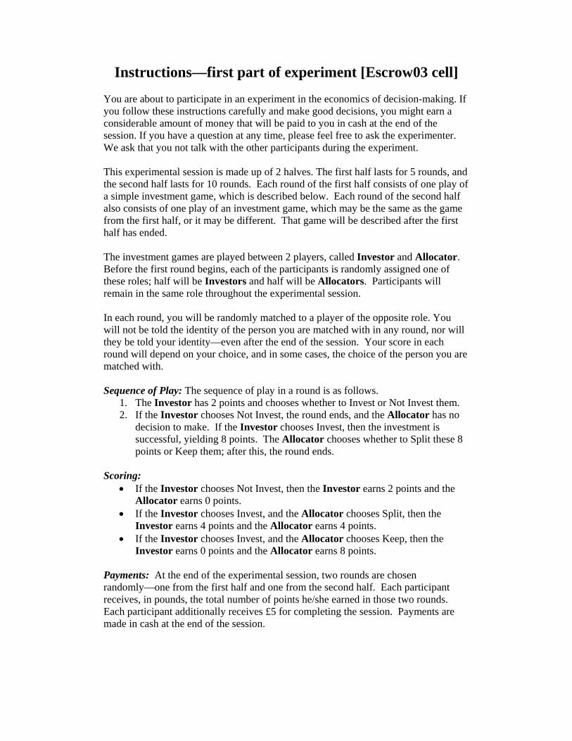
Instructions—first part of experiment [Escrow03 cell] You are about to participate in an experiment in the economics of decision-making. If you follow these instructions carefully and make good decisions, you might earn a considerable amount of money that will be paid to you in cash at the end of the session. If you have a question at any time, please feel free to ask the experimenter. We ask that you not talk with the other participants during the experiment. This experimental session is made up of 2 halves. The first half lasts for 5 rounds, and the second half lasts for 10 rounds. Each round of the first half consists of one play of a simple investment game, which is described below. Each round of the second half also consists of one play of an investment game, which may be the same as the game from the first half, or it may be different. That game will be described after the first half has ended. The investment games are played between 2 players, called Investor and Allocator. Before the first round begins, each of the participants is randomly assigned one of these roles; half will be Investors and half will be Allocators. Participants will remain in the same role throughout the experimental session. In each round, you will be randomly matched to a player of the opposite role. You will not be told the identity of the person you are matched with in any round, nor will they be told your identity—even after the end of the session. Your score in each round will depend on your choice, and in some cases, the choice of the person you are matched with. Sequence of Play: The sequence of play in a round is as follows.

1. The Investor has 2 points and chooses whether to Invest or Not Invest them. 2. If the Investor chooses Not Invest, the round ends, and the Allocator has no

decision to make. If the Investor chooses Invest, then the investment is successful, yielding 8 points. The Allocator chooses whether to Split these 8 points or Keep them; after this, the round ends.

Scoring:

• If the Investor chooses Not Invest, then the Investor earns 2 points and the Allocator earns 0 points.

• If the Investor chooses Invest, and the Allocator chooses Split, then the Investor earns 4 points and the Allocator earns 4 points.

• If the Investor chooses Invest, and the Allocator chooses Keep, then the Investor earns 0 points and the Allocator earns 8 points.

Payments: At the end of the experimental session, two rounds are chosen randomly—one from the first half and one from the second half. Each participant receives, in pounds, the total number of points he/she earned in those two rounds. Each participant additionally receives £5 for completing the session. Payments are made in cash at the end of the session.

Instructions—second part of experiment [Escrow03 cell] The procedure in this half of the experiment is very similar to that in the first half. Your role will be the same as in the first half. In each round, you will be randomly matched to a player of the other role. The only difference is that the investment game has an additional stage. Before the Investor makes a choice, the Allocator chooses whether or not to put 3 points into an escrow account. Rules of the escrow account:

• If the Investor chooses Not Invest, the escrow amount is returned to the Allocator.

• If the Investor chooses Invest, and the Allocator chooses Split, the escrow amount is returned to the Allocator.

• If the Investor chooses Invest, and the Allocator chooses Keep, the escrow amount is lost. (Neither player receives it.)

• Putting the 3 points into the escrow account is voluntary. The sequence of play in a round is now as follows.

0. The Allocator chooses whether to Escrow or Not Escrow. 1. The Investor sees whether the Allocator has chosen Escrow or Not Escrow,

then chooses whether to Invest or Not Invest the 2 points. 2. If the Investor chooses Not Invest, the round ends, and the Allocator has no

further decision to make. If the Investor chooses Invest, then the investment is successful, yielding 8 points. The Allocator chooses whether to Split these 8 points or Keep them.

3. The escrow amount (if any) is lost if the Allocator chose Keep. Otherwise, the escrow amount (if any) is returned to the Allocator.

Scoring:

• If the Investor chooses Not Invest, then the Investor earns 2 points and the Allocator earns 0 points (regardless of whether the Allocator chose Escrow or Not Escrow).

• If the Investor chooses Invest, and the Allocator chooses Split, then the Investor earns 4 points and the Allocator earns 4 points (regardless of whether the Allocator chose Escrow or Not Escrow).

• If the Investor chooses Invest, and the Allocator chooses Keep, then the Investor earns 0 points. The Allocator earns 8 points if he/she had chosen Not Escrow, or 5 points if he/she had chosen Escrow.