This paper presents preliminary findings and is being distributed to economists

and other interested readers solely to stimulate discussion and elicit comments.

The views expressed in this paper are those of the authors and do not necessarily

reflect the position of the Federal Reserve Bank of New York or the Federal

Reserve System. Any errors or omissions are the responsibility of the authors.

Federal Reserve Bank of New York

Staff Reports

Echoes of Rising Tuition in Students’

Borrowing, Educational Attainment, and

Homeownership in Post-Recession America

Zachary Bleemer

Meta Brown

Donghoon Lee

Katherine Strair

Wilbert van der Klaauw

Staff Report No. 820

July 2017

Echoes of Rising Tuition in Students’ Borrowing, Educational Attainment, and

Homeownership in Post-Recession America

Zachary Bleemer, Meta Brown, Donghoon Lee, Katherine Strair, and Wilbert van der Klaauw

Federal Reserve Bank of New York Staff Reports, no. 820

July 2017

JEL classification: D14, E24, R21

Abstract

State average enrollment-weighted public college tuition and fees per school year rose by $3,843

(or 81 percent) between 2001 and 2009. How are recent cohorts absorbing this surge in college

costs, and what effect is it having on their post-schooling consumption? Our analysis of tuition,

educational attainment, and debt patterns for nine youth cohorts across all fifty states indicates

that the tuition hike accounted for $1,628, or about 30 percent, of the increase in average student

debt per capita among 24-year-olds between 2003 and 2011. However, estimates indicate no

meaningful response to tuition on college enrollment, years of post-high school schooling, and

BA degree attainment rates. Our findings are consistent with American youth having

accommodated tuition shocks not by forgoing schooling, but instead by amassing more debt.

They signal an active role for the U.S. student loan system in shielding young Americans’ human

capital investments against shocks to (students’) education costs. Further analysis demonstrates

that the tuition hike and student debt increase, despite leaving higher educational attainment

unchanged, can explain between 11 and 35 percent of the observed approximate eight-

percentage-point decline in homeownership for 28-to-30-year-olds over 2007-15 for these same

nine cohorts. The results suggest that states that increase college costs for current student cohorts

can expect to see a response not through a decline in workforce skills, but instead through weaker

spending and wealth accumulation among young consumers in the years to come.

Key words: homeownership, student loans, household formation

_________________

Lee, Strair, and van der Klaauw: Federal Reserve Bank of New York (emails:

donghoon.lee@ny.frb.org, wilbert.vanderklaauw@ny.frb.org). Bleemer: University of California

at Berkeley (email: bleemer@berkeley.edu). Brown: Stony Brook University (email:

meta.brown@stonybrook.edu). The authors thank Andrew Haughwout, Henry Korytkowski of

Equifax, Anthony Orlando, and Joelle Scally; seminar participants at the Federal Reserve Bank of

New York, the Ohio State University, the Consumer Financial Protection Bureau, Baruch

College, and the Urban Institute; and conference participants at the FDIC Consumer Research

Symposium, and Goldman Sachs’ Millennials and Housing Day for valuable comments. The

views expressed in this paper are those of the authors and do not necessarily reflect the position

of the Federal Reserve Bank of New York or the Federal Reserve System.

1

The circumstances of young American consumers have undergone three unprecedented

changes since the start of the twenty-first century. First, student loan balances and the prevalence

of student borrowing have reached new heights, with the nominal aggregate student debt

reflected in the New York Fed’s Consumer Credit Panel (CCP) growing from roughly $360

billion in 2004 to $1.2 trillion in 2016, and the prevalence of student borrowing by age 25 rising

from 25 percent in 2004 to nearly 45 percent by 2016. Second, homeownership rates among

young consumers fell drastically following the recession, with age 30 homeownership dropping

from 31 percent in 2004 (and 32 percent in 2007) to 21 percent by 2016.1 Finally, the share of

young consumers living with parents or similar elders has climbed dramatically. While 33.5

percent of 23 and 25-year-olds lived with parents or similar elders in 2004, 44.9 percent lived

with parents or similar elders by 2015.

Given the evidence, and the usual life-cycle timing of student and mortgage borrowing,

one might wonder what the relationship is among the cost of education, student borrowing, and

subsequent housing choices. Public and private college costs have grown alongside student

borrowing.2 Figure 1 depicts enrollment-weighted mean tuition and fees at four-year public

colleges and universities for each state from 2001 to 2009.3 The figure demonstrates the steep

growth in college costs over the period: the mean across states of enrollment-weighted state

average tuition and fees per school year increased by $3,843, or 81 percent, from 2001 to 2009.

It also demonstrates a substantial increase in dispersion across states in enrollment-weighted

average tuition and fees, with the range of state averages increasing from $2,788-$12,893 in

2001 to $3,671-$20,466 in 2009. To the extent that the cost of a given human capital investment

has increased, younger cohorts might be expected to experience some disadvantage in the shared

housing market. Moreover, to the extent that student debt repayment struggles are increasingly

prevalent, and mortgage underwriting is tighter following the Great Recession, young consumers

1 These homeownership rates are measured in the CCP data at the level of the individual fileholder. Household-level

homeownership rates are slightly higher, but experienced a similarly sharp decline. 2 See, for example, Oliff, Palacios, Johnson, and Leachman (2013), on state university funding before and after the

Great Recession. 3 Throughout the paper we emphasize the tuition growth from 2001 to 2009, though of course data are available for

more recent years, and some are presented in Figure 1. The 2001-2009 tuition increase is one segment of a much

longer trajectory. See, for example, College Board (2016) on the steady growth of real tuition and fees from the

1970s through 2010. The cohorts in college from 2001-2009 are those whose recent homeownership choices, from

2007 to 2015, we study below. Current cohorts of students and very recent tuition growth are certainly of interest,

but we have no evidence yet on these cohorts’ graduation rates and post-schooling experiences.

2

who manage increased college costs by borrowing might be expected to experience decreased

mortgage access.4

This paper asks how the rapid increase in college costs has affected recent youth cohorts’

student borrowing, educational attainment, and post-schooling consumption. As the price of

higher education grows, do students choose to forego schooling or to meet the higher price of

schooling with the aid of student debt? If the latter, what relationship do we observe between

such tuition-induced debt and young Americans’ lives after college?

Given the evidence of the challenges inherent in measuring student loan dollars in a

survey context that we present in Brown et al. (2016), along with evidence of a strong negative

association between students’ ability to report balances and their subsequent homeownership, we

turn to the Equifax-sourced New York Fed Consumer Credit Panel (CCP) for administrative data

on the college borrowing and later homeownership decisions of nine recent cohorts of young

American consumers. The CCP is valuable in this context for its ability to provide administrative

data on student borrowing at age 24 and, four to six years later, homeownership at ages 28, 29

and 30 for nine distinct birth cohorts. Homeownership measures are drawn from 2007 to 2015,

representing the recession and post-recession period. The CCP’s large sample size and fine

geography allow us to track local borrowing and homeownership patterns at individual ages –

homeownership at 28, 29, and 30, for example – rather than in age bands. These can be measured

in sufficient sample sizes across all fifty states throughout the estimation window.

The primary limitation we encounter with the CCP is its lack of education measures, a

feature of credit reports in general. To analyze behavioral responses in educational attainment we

draw on individual-level data from the Integrated Public Use Microdata Series (IPUMS). In

addition to college enrollment and Bachelor’s degree attainment, it includes the total years of

post-high school education for each individual in the IPUMS data belonging to the same 1979-

1987 birth cohorts we study in our CCP-based analysis.

Data drawn from the US Department of Education’s Integrated Postsecondary Education

Data System (IPEDS) reflect the cost of college faced by a state-cohort, by age 22. In the CCP,

4 One mechanism by which student loan dollars may influence the transition to homeownership is through total debt-

to-income (DTI) ratios used in mortgage underwriting. Recent reforms have aligned the underwriting standards of

FHA and Fannie Mae to include the greater of the student loan payment or one percent of the outstanding loan in the

DTI calculation made in underwriting a mortgage (see, for example, U.S. Department of Housing and Urban

Development (2016), Mayotte (2016)). Each had stood at two percent at some point in the recent past, though the

FHA had long disregarded student debt in its DTI calculation before the recession.

3

we measure the student debt accumulated by age 24, and the homeownership rates of 28-, 29-,

and 30-year-olds, for each individual belonging to the included birth cohorts.

While our analyses are based on individual-level data, the college tuition paid by a given

youth at her chosen school is likely endogenous to her later homeownership. For causal inference

we therefore rely on aggregate state- and cohort-level variation in tuition. After accounting for

persistent difference across states and time, we treat remaining variation due to differences in the

timing and magnitudes of tuition increases as plausibly exogenous. Furthermore, our estimated

relationships account for broader state and time patterns, and data from additional outside

sources inform the empirical model regarding the state of relevant time-varying economic

circumstances in each location.

Hence, we use variation within and between U.S. states in the college tuitions faced by

different schooling cohorts to relate both student borrowing and college attendance and

educational attainment levels to college costs, and then to relate post-schooling homeownership

to college costs and tuition-induced increases in student debt. Our estimates first address the

question of how students respond to the rising cost of education: by dropping out, or by

borrowing more?5 Our empirical model indicates that the per-capita $3,578 increase in states’

mean enrollment-weighted public tuition per school year from 2001 to 2009, is associated with a

$1,628 increase in per capita student debt among (all) 24-year-olds.6 However, we find no

change in educational attainment, whether measured by years of post-secondary education,

college enrollment or BA degree attainment by age 24 associated with this increase in tuition.

These results suggest that American students’ price elasticity of demand for higher education is

quite low. As college costs increase, American students do not forego education, but instead

amass more debt.

Following these same nine cohorts six to eight years past their (traditional) college years,

and four to six years past the age 24 student loan comparisons, we examine the rate at which

each cohort achieves homeownership by ages 28, 29, and 30. Relative to the 2001 age 22 cohort,

the mean age 28 to 30 homeownership rates for the 2009 age 22 cohort is approximately 7.74

5 Other means of accommodating a tuition hike are available. As the price of education rises, students will consume

less of it and spend more on it, in some combination. Non-borrowing means of spending more include working more

while in college and extracting more financial support from families. 6 Note that the per-capita increase in tuition and fees of $3,578 is slightly lower than the mean state-level tuition and

fees increase of $3,843, discussed earlier, reflecting larger tuition hikes in less populated states.

4

percentage points lower, on a base of 26.91 percent7. Exploiting state-cohort level variation in

tuition in a fixed effects specification, we estimate the response of homeownership at these ages

to the $3,578 average tuition increase for the same cohorts between 2001 and 2009. According to

our estimates, the 2001-2009 tuition increase can explain 0.84 percentage points of the 7.74

percentage point decline (or 11%). As discussed in more detail in Section III, while we cannot

exclude the possibility that the rise in tuition may have affected homeownership through

channels other than increased student debt, the debt channel is likely to be predominant. When

we adopt a standard instrumental variables (IV) approach that attributes all of tuition’s impact on

homeownership to its effect through student debt, the estimates imply a strong negative impact

of student debt on homeownership, with a $1,000 increase in average student loan debt leading

to a 0.48 percentage point reduction in the homeownership rate at ages 28 to 30. This estimate

implies that the observed $5,707 increase in mean per capita student debt from 2003 to 2011

could explain 2.74 percentage points of the overall 7.74 percentage point, or 35% of the decline

in homeownership at ages 28 to 30.

Policy inferences arising from our quasi-experimental evaluation, in the absence of a

behavioral model in which to draw welfare conclusions, must be tempered. That said, our

evidence is consistent with the claim that American students have absorbed substantial college

tuition shocks, without lowering their human capital investment, through an increasing reliance

on the U.S. student loan system. Those who might respond to news of greater aggregate student

debt, and of ubiquitous student loan delinquency and default, by reducing students’ access to

loans should consider this evidence. Contained within it is the suggestion that, absent recourse to

student loans, young Americans might at last respond to rising college tuitions by purchasing

less education.

Assuming stability in our student loan system, others might infer that, because the

estimated response to tuition hikes appears in the form of student borrowing and not in the form

of declining schooling, the de-funding of public higher education has been a success. States are

spending substantially less, per taxpayer, on higher education, and yet the skill of the workforce

remains unaltered. Our homeownership estimates suggest that the de-funding of higher education

7 In computing these rates, we have accounted for the fact that for the 2002 cohort we only observe homeownership

at ages 28 and 29, and for the 2001 cohort only at age 28, as discussed in more detail below.

5

has not been costless, at least in the context of one spending channel. Moreover, homeownership

represents an important means of wealth accumulation, with housing equity being the principal

form of wealth for most households. States that increase the cost of education therefore may pay

a price not in the form of declining workforce skill, but instead through muted housing-related

spending and lower wealth accumulation among younger consumers in the years to come.

The paper proceeds as follows. In section I, we discuss the economic developments that

characterize our estimation period in more detail, including trends in U.S. college costs, student

borrowing, co-residence with parents, and early homeownership. We then summarize the related

literature. Section II turns to administrative data on student borrowing and homeownership

drawn from the CCP. It describes the construction of the aggregated dataset, along with

additional empirical sources. Section III details our empirical approach, and summarizes findings

regarding the relationship among college cost, student borrowing, educational attainment, and

early homeownership.

I. Context: Economic developments and related literature

a. Developments from 2001 to 2015 in young Americans’ college costs, student borrowing, and

living arrangements

The three unprecedented changes in the circumstances of young Americans over the early

21st century that we describe in the introduction are reflected in young Americans’ balance

sheets. From 2003 to 2015, we observe a modest overall decline in the debt held by 30-year-olds

in the CCP. But more striking is their reallocation of debt over that time. In real terms, the credit

report of a representative 30-year-old in 2015 shows 28 percent less home-secured debt, 6

percent less auto debt, and 36 percent less credit card debt than that of a 30-year-old in 2003. It

shows 174 percent more student debt.8 Today’s young Americans exhibit a radically different

relationship to both housing and consumer debt markets than that of young Americans only

twelve years ago. Importantly, this change does not represent a broader pattern in American

consumer behavior. Older Americans are borrowing more from nearly all standard sources: the

credit report of a representative 65-year-old in 2015 includes 47% more housing debt,

approximately identical credit card debt, 29% more auto debt, and more than an eight-fold

8 This evidence is based on the authors’ calculations using the CCP, and appears in Brown, Lee, Scally, and van der

Klaauw (2016). Related evidence can be found in Demyanyk and Kolliner (2015) and Brown and Caldwell (2013).

6

growth in student debt when compared with a representative credit report for a 65-year-old in

2003.9 As older Americans have borrowed more from (almost) all sources, younger Americans

have both borrowed less and shifted their borrowing aggressively toward the student loan

market.

Repayment proves challenging for the majority of student borrowers, in one way or

another. Figure 2 describes the repayment experiences of the 2009 school-leaving cohort as of

the end of 2014.10

Here we see that the prevalence of explicit repayment failures, in the sense of

default or delinquency exceeding 120 days, is highest for the smallest balance borrowers, at 51

percent. From there, the rate of repayment failure first declines and then eventually flattens as

student debt balances increase. Further, if one includes not having paid down a dollar of the 2009

school-leaving balance by the end of 2014, the prevalence of repayment problems takes on a u-

shape. Repayment struggles are very common among low-balance borrowers, at 59 percent

among the $1000-5000 2009 balance group, and among high-balance borrowers, at 57 and 54

percent among the $50,000-$100,000 and $100,000+ groups, respectively. The most successful

repayers are those with 2009 balances between $10,000 and $25,000, but even among those 48

percent have defaulted, been severely delinquent, or not repaid a dollar as of late 2014.

Dynarski (2016) provides evidence of declining student loan default rates as a function of

past balance, and Dynarski and Looney and Yannelis (2015) describe the relationship of this

surprising negative association to the post-college earnings of large and small borrowers. We

find this discussion to be of substantial value to the literature, and here add the observation that,

where small borrowers struggle with delinquency, large borrowers manage to remain nominally

current and yet fail to repay. Perhaps most importantly, something about the repayment

experience leaves 48 percent of even the most successful repayment group, the mid-range

borrowers, struggling.11

9 These comparisons are made in 2015 dollars. Average home-secured debt at 30 fell by $8,195, or 28%; at 65 it

increased by $11,191, or 47%. Average credit card debt at 30 fell by $1,121, or 36%; at 65 it fell by $11, which

rounds to 0%. Average auto debt at 30 fell by $292, or 6%; at 65 it grew by $1102, or 29%. Average student debt at

30 grew by $6,912, or 174%; at 65 it grew by $857, or 886%. 10

Figure 1 was first published in Brown, Haughwout, Lee, Scally, and van der Klaauw (2015b). The school-leaving

cohort is determined based on the last quarter in which we observe student borrowing for the consumer in the CCP. 11

It is worth noting that the 2009 school-leaving cohort demonstrates somewhat worse five-year repayment

outcomes than those shortly preceding it, for obvious reasons. The relative CCP five-year cohort default rates of the

2005, 2007, and 2009 school-leaving cohorts give some idea of the magnitude of the business cycle contribution to

the prevalence of repayment troubles. Brown, Haughwout, Lee, Scally, and van der Klaauw (2015a) find these rates

to be 20, 21, and 26 percent, respectively.

7

As reliance on the U.S. student loan system advanced, younger Americans’ residential

circumstances also underwent a transformation. Figure 3 shows homeownership rates at ages 28,

29 and 30 by age-22 cohort. We infer homeownership based on the presence of home-secured

debt, whether mortgage or home equity-based loans, on the sample member’s credit report. The

presence of home-secured debt on the credit report is a particularly reliable proxy for

homeownership at young ages, and its absence a reliable proxy for non-homeownership, as very

few 28-30-year-old homeowners in the U.S. own their homes outright.12

We find that

homeownership among 28-year-olds declined steadily from 24.4 percent in 2007 to 16.0 percent

in 2015, an approximate 0.94% annual decline. We see a similar decline for homeownership at

age 29 (0.91% annual) and a slightly smaller decline at age 30 (0.74 annual rate).

Finally, as homeownership declined, young Americans increasingly chose to live with

their parents or with similar elders. Figure 4 depicts the proportion of U.S. 23-25-year-olds living

with “parents” in the CCP from 2004-2015. For 23-25 year old CCP sample members, we

observe an increase in the rate of co-residence with parents or similar elders from 33.5 percent in

2004 to 44.9 percent in 2015.13

Note that this pattern is free of life-cycle effects, as we measure

co-residence with parents for the cross-section of CCP sample members who are 23 and 25 years

old in each year. This substantial growth in living with parents is approximately monotonic over

the period, and proceeds at a steady pace from 2004 to 2015.

b. Related literature

A number of studies have investigated whether and to what extent the observed empirical

relationship between student debt and homeownership represents a causal relationship. Such an

investigation is complicated by the presence of confounding factors: individual- and household-

level attributes and circumstances that influence both the amount of student debt taken out as

well as directly affecting subsequent home purchase decisions. Perhaps foremost amongst these

is the education itself for which the debt was incurred. Those with positive and larger amounts of

student debt are likely to have attained a higher level of educational attainment, in quantity or

12

Similar results obtain where we track the rate of ever owning over the full course of the panel. The potential

difficulty with this measure is that the look-back window available in the CCP lengthens as the panel progresses,

creating time dependence in the quality of the measure of homeownership. 13

We adopt the phrase “living with parents” to describe youth living with parents or with one of the variety of

responsible elders captured by our co-residence measure, which defines co-residence as residing at the same street

address as at least one individual who is between 15 and 45 years older.

8

quality, than those with no or less debt, resulting in higher subsequent earnings, wealth and home

ownership. Parental income and academic ability similarly are factors likely to both influence

student debt and homeownership. Several confounding factors, such as ambition, preferences and

parental support, may be hard to measure. A failure to adequately account for such confounding

factors is then likely to result in invalid inferences.

In the face of such challenges in empirically identifying a causal relationship, one fruitful

approach might be simply to ask student borrowers whether their loans have affected their

homeownership choices. A number of post-recession surveys provide decisive evidence that

young consumers feel their progress toward ownership is slowed by their student debt. In a 2011

Pew Research Center survey of a nationally representative sample of American adults, 48

percent of student borrowers responded that student debt made it harder to pay other bills, and 25

percent said that student debt has made it harder to buy a home (Pew Research 2011). The

National Association of Realtors (NAR) publishes the results of an annual survey of homebuyers

regarding market conditions and their experiences. Among buyers aged 18-35, 44 percent held

student debt at the time of the homebuyer survey, with a median outstanding balance of $25,000.

Further, 53 percent of buyers in this age group reported that they had been delayed by student

debt in purchasing a home (NAR 2016). In a 2013 American Student Assistance (ASA) survey

of 259 young professionals, 75 percent reported that student debt had affected their ability to

purchase a home (ASA 2013). Additionally, 59 percent of those with student debt reported

difficulty making student loan payments, 60 percent reported confusion with student loan

repayment paperwork, and 69 percent reported confusion regarding repayment options. Finally,

the third annual America at Home survey in 2015, a national telephone survey fielded by

NeighborWorks America, showed an increase in the rate at which respondents reported that

student loan debt is “at least somewhat of an obstacle to buying a home”. Fifty-seven percent of

respondents agreed with this statement in 2015, up from 49 percent in 2014.

Research on the effect of student debt on post-schooling outcomes using more conventional

survey data and methods has generated mixed results. This heterogeneity in findings is likely to

reflect at least in part cross-study variation in the effectiveness of approaches to account for

confounding factors. Findings from several studies using survey data appear to suggest modest or

no effects of student debt. Kurtz and Li (2015), using the Consumer Expenditure Survey, find

that the likelihood of purchasing a vehicle is, in fact, increasing in the ratio of student debt to

9

income. Exceptions appear for the cases of student borrowers with very high balances, and for

the case of cash purchases of new vehicles. Akers and Chingos (2014), using a long series of

waves from the Survey of Consumer Finances (SCF), find that the homeownership rates of

student borrowers relative to those of non-borrowers have waxed and waned over the years, and,

further, that the debt payments that SCF household heads report that student borrowers actually

make constitute, at the median, roughly 3-4 percent of monthly income. They conclude that the

payments that student borrowers are making are not burdensome relative to their incomes, which

reflect the returns to their educational investments. Houle and Berger (2015) study

homeownership rates in the NLSY’s 1997 cohort. They find a modestly lower homeownership

rate among student borrowers than among non-borrowers, but no significant association between

student loan balance and homeownership. Instead, they find that sociological markers of the

transition to adulthood are substantially positively associated with homeownership.

While the aforementioned studies find little evidence of large impacts of increased student

debt, Gicheva and Thompson (2015), using the SCF, find significantly higher rates of binding

credit constraints and bankruptcy following schooling for student borrowers than for non-

borrowers, and some evidence of lower homeownership among student borrowers. Gicheva

(2016) finds a negative association between student debt and subsequent first marriage rates in a

survey of registrants for the Graduate Management Admissions Test, controlling for other

relevant factors. Cooper and Wang (2014), using the Panel Study of Income Dynamics, find that

student debt is associated with a lower likelihood of homeownership by age 30 for a group of

individuals who attended college during the 1990s. Further, Cooper and Wang observe a fairly

strong negative association between student loan debt and wealth for a group of households who

have at least some college experience and a household head aged 40 or younger.

In a related paper, Brown, Hunter, Lee, and van der Klaauw (2016), we study student

borrowing and later homeownership in the National Longitudinal Survey of Youth’s 1997

cohort. Its 1997 adolescents reached age 30 between 2010 and 2014, which provides us the

opportunity to study post-recession homeownership at age 30 among five consecutive birth

cohorts, whose education, family background, financial resources and choices, academic ability,

and post-schooling experiences have been meticulously documented from the age of 12-16

forward. Among our findings in the paper, perhaps the most novel and the most relevant to the

analysis here pertains to survey data quality and the role of students’ financial awareness.

10

Conditioning on measures of ability, diligence, background, family supportiveness, final

educational attainment, and a host of other relevant characteristics, we estimate that, among

student borrowers able to report loan balances, $10,000 in additional student debt accumulated

during school is associated with a 1.49 percentage point decline in the probability of

homeownership at age 30. At the same time, we find that a substantial minority of student

borrowers fail to report balances, and that student borrowers who cannot report their loan

balances have similar homeownership rates to borrowers who report $36,000 of cumulative

borrowing. This amount is roughly three standard deviations above the mean cumulative balance

among student borrowers. Alternatively, the estimates show borrowers unable to report balances

to be 5.4 percentage points less likely to own homes at age 30 than otherwise comparable non-

borrowers. The estimated relationship between age 30 homeownership and the inability to report

student loan balances is as strong as or stronger than all other estimates in the paper that describe

the relationship between student loan history and later homeownership.14

These findings suggest two things about survey data on student debt: First, inferences based

on survey data involving student loan balances should be treated with caution, given the apparent

importance of limitations in respondents’ ability to report balances. This observation motivates

our use of administrative data in the present study, as lender-reported balances avoid any

limitations affecting borrowers’ financial awareness and willingness to report. Second, only

survey data allow the researcher to identify the subset of borrowers who have limited knowledge

of their debt (or limited willingness to report). Hence, unlike administrative data, survey data

have the potential to inform us regarding whether borrowers with limited financial awareness are

bearing the brunt of the student loan repayment failures described in Section I.a.

One independent and contemporaneous study of the causal impact of student borrowing on

later homeownership uses comprehensive administrative data merged from credit bureau,

Department of Education, and other sources. As we do in our paper, Mezza, Ringo, Sherlund,

and Sommer (2016) turn to tuition-induced variation in student debt across time and states to

analyze the relationship between student debt and homeownership. They have assembled a

powerful data resource, merged from several administrative sources, that includes not only

14

This evidence is in line with the results of a comparison of administrative and survey data on U.S. student debt

balances in Brown, Haughwout, Lee, and van der Klaauw (2015), in which the aggregate student loan balance

implied by borrower-reported survey data was estimated to be, at most, 75 percent of the aggregate balance implied

by lender-reported administrative data.

11

student and housing debt histories following schooling, but also detailed educational histories for

the 5,610 American students with non-zero student loan balances that constitute their estimation

sample. Their estimates indicate that a 10% increase in student debt leads to a 1 to 2 (1 to 1.5)

percentage point decrease in the probability of homeownership two (five) years out of school.

However, several aspects of the Mezza et al. study distinguish it from ours. First, it is

important to note that the findings of the study are based on students who left school between

1997 and 2005. Given the tightening of mortgage underwriting standards after 2008, one could

expect student debt to have become an even greater drag on homeownership for subsequent

cohorts of school-leaving students. In addition, the study relates homeownership to differences in

student loan balances only among those youth who borrow positive amounts. It does not address

the extensive margin of student debt growth. From 2003 to 2011, we observe an increase in the

proportion of 25-year-olds whose credit reports include student debt from 0.25 to 0.42, an

increase in the prevalence of student borrowing of 68 percent. Whether this change reflects

increasing enrollments or more enrolled students moving into borrowing due to escalating

college costs, such a large change in student debt market participation, in addition to the growth

in balances among borrowers, could influence later homeownership.

As explained later in section III, another feature of the study is that it relies on a strong

exclusion restriction, where tuition is only allowed to affect later home-ownership choices

through its effect on student debt (and not, for example, through a change in the quality of

education attained, an impact of increased employment while in college, and of an increased

reliance on financial support from families), and also relies on the assumed exogeneity of

included controls such as the level of education attained.

Though we lack the elaborate, merged administrative data on educational and personal

characteristics that make the Mezza et al. study uniquely informative, we are able to address the

question of the relationship among college costs, student borrowing, and subsequent

homeownership for more recent cohorts, including several post-recession cohorts, to estimate

homeownership responses at somewhat older ages, to estimate using a sample of millions of

American youth, and to harness the observed growth in both the extensive and intensive margins

of student borrowing.

In doing so, we take an approach that differs in another important aspect from previous

studies by focusing more directly on the role of rising college cost as a cause of increased student

12

debt. Observed changes in student debt levels reflect changes in consumer demand for education

(quantity as well as quality), application behavior and admission policies, available family

resources, financing options, needs and costs. Our analysis will focus on changes in the price of

education as a specific primitive cause of increased student debt, and address the following

policy questions: How do students respond to the rising cost of education: by not enrolling in

college or dropping out, or by borrowing more? What, if any, impact did the sharp rise in college

costs have on educational attainment as measured by college attendance, BA degree attainment

and total years of education? How much of the observed growth in student debt is attributable to

the increase in college costs as measured by state tuition levels? And to what extent is the sharp

decline in homeownership among younger Americans attributable to the rise in college costs, and

the associated increase in student debt?

Given its focus on the price of a college education, our analysis is informative about the

causal impact of policy-induced shifts in the financing of college education away from state and

federal governments towards students and their families. Thus, instead of trying to assess what

the homeownership rate would be in absence of the student loan program, or of analyzing the

impact of variation in student debt irrespective of its source, we consider what we take to be the

more relevant policy question of what the homeownership rate of younger Americans would

have been if average college tuition (and associated student debt) had not grown or grown by a

different amount in recent years.

II. Data sources and measurement

a. Administrative debt data: The FRBNY Consumer Credit Panel

The New York Fed Consumer Credit Panel is a longitudinal dataset on consumer

liabilities and repayment. The data include individual account-level information on all

mortgages, home equity lines of credit, and student loans, as well as information on all credit

card and auto loan debt. The panel is built from quarterly consumer credit report data collected

and provided by Equifax Inc. Data have been collected quarterly since 1999Q1, and the panel is

ongoing.15

Sample members have Social Security numbers ending in one of five arbitrarily

selected, randomly assigned pairs of digits. Therefore the sample comprises 5 percent of U.S.

individuals with credit reports (and Social Security numbers). The CCP sample design

15

Student debt data are only available in the CCP starting in 2003.

13

automatically refreshes the panel by including all new reports with Social Security numbers

ending in the above-mentioned digit pairs. Therefore the panel remains representative for any

given quarter, and includes both representative attrition, as the deceased and emigrants leave the

sample, and representative entry of new consumers, as young borrowers and immigrants enter

the sample.16

While the sample is representative only of those individuals with Equifax credit reports, the

coverage of credit reports (that is, the share of individuals with at least one type of loan or

account) is fairly complete for American adults. Aggregates extrapolated from the data match

those based on the American Community Survey, Flow of Funds Accounts of the United States,

and SCF well.17

However, because we focus on young people’s student borrowing and

homeownership decisions, we restrict our dataset to 24- to 30-year-olds, who have lower

coverage than later ages; CCP coverage over 2003-2013 of the Census-estimated, age-specific

population ranges between 83.4 and 93.9% for 25-year-olds and between 91.0 and

(approximately) 100% for 30-year-olds, increasing from 2003 to 2007 and decreasing from 2007

to 2013.18

We construct an individual-level, pooled dataset from the CCP by first extracting

observations for all individuals who are between 24 and 30 years old in each panel year between

2003 and 2015.19

Because the pooled-panel aspect of our study drastically increases the number

of observations, we only pull a random 1% sample of the covered U.S. population, instead of the

full CCP 5%. In total, we estimate with a pool of 774,794 individual-year observations. In order

to align our estimates of the tuition-student debt and tuition-homeownership relationships with

those from the tuition-educational attainment model, we similarly construct samples from the

2003-2011 IPUMS of individuals aged 24 belonging to the 1979-1987 birth cohorts.

Using the CCP’s loan-level student debt balance data, we calculate the total student debt

held by each 24-year-old in our pooled estimation sample. Since CCP student loan data begin

16

See Lee and van der Klaauw (2010) for details on the sample design. 17

See Lee and van der Klaauw (2010) and Brown et al. (2015) for details. 18

Lee and van der Klaauw (2010) extrapolate similar populations of U.S. residents aged 18 and over, overall and by

age groups, using the CCP and the ACS, suggesting that the vast majority of US individuals at younger ages have

credit reports. Jacob and Schneider (2006) find that 10 percent of U.S. adults had no credit reports in 2006, and

Brown et al. (2015b) estimate that 8.33 percent of the (representative) Survey of Consumer Finances (SCF)

households in 2007 include no member with a credit report. They also find a proportion of household heads under

age 35 of 21.7 percent in the 2007 SCF, 20.64 in the 2007Q3 CCP, and 20.70 from Census 2007 projections,

suggesting good representation of younger households in the CCP. 19

We use data for the fourth quarter of each year of the panel.

14

with 2003, our student loan measures cover only birth cohorts that reached age 24 in 2003 or

later. Note that the oldest cohort in our sample, then, reaches age 28 during 2007. Hence our age

28 to 30 homeownership outcome measures span the period of available data on homeownership

for cohorts with valid student debt data, from 2007 through 2015. The measure of home

ownership used in the estimates is an indicator for whether the fileholder holds any home-

secured debt at the age in question (28, 29, or 30), as discussed above.

b. Other data sources

Annual county-level employment data are drawn from the Bureau of Labor Statistics’

(BLS) Quarterly Census of Employment and Wages (QCEW) program. The employment data

are reported on a quarterly basis, and they cover a total of 3,197 counties. In order to measure the

employment-to-population ratio, we also draw annual county-level population data from the US

Census’s Population Estimates.20

We calculate the youth unemployment rate at the state level

using employment data from 18- to 30-year-old individuals drawn from the Current Population

Survey (CPS), aggregated from months to quarters.21

Average weekly county-level wage data for

3,197 counties are also drawn from the BLS’s QCEW program. Finally, we calculate versions of

each of these measures for the county in which we observe each fileholder at age 22, and for the

year in which the youth turned 18. This allows us to account for local conditions during or

leading up to the time that the state tuition applicable to the cohort was determined.

The mean student debt per capita among 24-year-olds in our sample is $6,715 with a

mean of $3,902 in 2003 rising to a mean of $9,603 in 2011.

At the center of the analysis below is a set of college tuition measures. We construct a

series of state-cohort average sticker costs of public colleges by pulling cost data from IPEDS.22

We define sticker cost as the sum of tuition and fees (excluding room and board) at US public

colleges and universities. Costs are averaged across postsecondary public institutions by state,

sector, and year, and weighted by undergraduate enrollment. The average across the pool of all

state-cohorts in our sample of the mean state sticker cost of public college is $6,723 per school

20

Data are from the 1990s Postcensal Estimates and the Vintage 2009, 2014, and 2015 estimates. 21

This aggregated sample of the CPS (over all months from 2003 to 2015) includes 3.2 million respondents between

age 18 and 30—19,333 of whom are missing labor force status information—though due to the sampling

methodology of the CPS, some people appear in the dataset twice (in two different quarters). Data are aggregated

using individual weights. 22

IPEDS covers all 7,255 postsecondary schools in the United States, 5,126 of which provide enrollment and tuition

data, accounting for 97.8 percent of enrollment in the dataset.

15

year, with a standard deviation of $2,794.23

Our focus on tuition at public colleges and

universities is motivated by the fact that time-variation in this measure is more likely to capture

exogenous reflections of idiosyncratic political processes rather than market demand. Private

tuitions instead are set by private universities, likely in response to changes in demand for their

degrees (and tuition costs at public institutions). For similar reasons we prefer using the sticker

price rather than a net cost price. Net tuition would reflect differences and changes in average

household income levels (determining Pell grant eligibility), as well as potentially endogenous

college enrollment choices and grant allocation decisions by public colleges and universities.

III. Empirical specifications and results

a. Estimation of student debt and graduation choices

Our administrative data include rich detail on a young consumer’s location, age, and debt

portfolio. They do not, however, offer the level of detail regarding demographic characteristics

and human capital investment typical of survey data. Still, the present paper adds a new

perspective that the survey-based analysis cannot. First, it permits estimation using student debt

measures that are not affected by any shortcomings in student borrowers’ willingness or ability

to report balances. Second, the large sample and fine geographic data of the CCP allow us to

place the student borrowing and homeownership choices that we observe in local economic and

institutional context. Moreover, this context varies widely within our sample, owing to measures

taken for hundreds of thousands of young consumers over a broad and detailed geography and a

fairly long panel. Hence, while we cannot fix test scores or high school academic performance

for sample youth in modeling the dependence of educational outcomes on tuition, and of

homeownership on tuition and past student debt, we can compare the decisions of youth who are

members of state-cohort groups who were subject to higher and lower college costs. Moreover,

we can do so for youth who are experiencing expanding local economic conditions, as well as for

those struggling through local recessions.

While our analyses are based on individual-level data, our main source of identifying

variation in the tuition variable will operate at an aggregate state-cohort, rather than individual,

level. We restrict our sample to cohort-year pairs in which the cohort making the educational

23

Appendix Table A1 reports descriptive statistics for each variable used in the estimation, based on the state-

cohort-year cells.

16

choice in question is 24 years old, or the cohort making the housing choice in question is

between 28 and 30 years old. For each of these cohort-year pairs, we assemble overall

employment to population, mean wage, and other characteristics described above at the county

level for the specific cohort-year combination.

Hence we begin by estimating the following fixed effects model of education outcomes –

student debt, college attendance, years of education and BA degree attainment, each measured at

age 24 – for a sample of CCP youth cohorts whose tuition is observed between 2001 and 2009,

and whose education outcomes are observed between 2003 and 2011:

𝑌𝑖𝑐𝑙 = 𝑋𝑐𝑙𝑡𝛽 + 𝐸𝑐𝑠𝛾 + 𝛿𝑠 + 𝜏𝑐 + 휀𝑖𝑐𝑙, (1)

where 𝑌𝑖𝑐𝑙 represents the age-24 education outcome of individual i of youth cohort c residing in

county l in state s at age 22.24

Further, 𝑋𝑐𝑙𝑡 represents a vector of covariates that includes the

current (at time t and age 24) county employment-to-population ratio, drawn from the QCEW,

state youth unemployment rate, based on the authors’ calculations in the CPS, and current

county-level QCEW mean wage.

Vector 𝐸𝑐𝑠 represents the IPEDS-sourced, enrollment-weighted mean school-year tuition

and fees across all public colleges and universities in the state, as described above. This variable

is our regressor of primary interest. Note that by including state fixed effects (for the location at

which tuition is measured) we account for persistent differences across states in the quantity,

quality and cost of education, while by including cohort fixed effects we account for common

changes in these education measures over time. Moreover, we account for differences in current

local economic conditions. Thus for identification we rely purely on remaining differential state-

cohort variation in tuition, reflecting differences in the timing and magnitude of tuition increases

across states.

The properties of error term 휀𝑖𝑐𝑙 remain to be determined. While using individual-level

data on educational outcomes and county-variation in local economic conditions, we rely on

state-cohort-level tuition variation to estimate the relationship between tuition levels and

educational outcomes. One may therefore want to adjust the standard errors to account for

remaining serial correlation, even after estimating both state and cohort fixed effects. In sections

24

Estimates based on age 20-22 tuition averages provide similar estimates.

17

III.d.2 through III.d.4 below, we report estimates of expression (1) first under classical least

squares assumptions on the error term, next while clustering errors 휀𝑖𝑐𝑙 by individual i’s age-22

state (at which a cohort’s tuition is measured), and, finally, using Driscoll-Kraay (1998,

henceforth DK) standard errors. The DK estimator has a cluster interpretation- it is equivalent to

state-year clustering, along with use of the Newey-West method to account for serial correlation,

which allows for correlations that span different states and years (Foote, 2007).

b. Estimation of the association between college costs and early homeownership

Similarly, we estimate an aggregated fixed effects model of the dependence of

homeownership at age 28, 29, and 30 on tuition, or, alternatively, on the student debt

accumulated by the state-cohort at age 24. Here we measure tuition from 2001 to 2009, student

debt from 2003 to 2011, and, finally, the homeownership rate among younger consumers

between 2007 and 2015. The model in this case is:

𝑌𝑖𝑐𝑙𝑡𝐻 = 𝑋𝑐𝑙𝑡𝛽

𝐻 + 𝐸𝑐𝑠𝐻𝛾𝐻 + 𝛿𝑠

𝐻 + 𝜏𝑐𝑡𝐻 + 휀𝑖𝑐𝑙𝑡

𝐻 , (2)

Where 𝑌𝑖𝑐𝑙𝑡𝐻 represents an indicator for whether individual i of cohort c residing in county l at

time t (age t-c) owns a home that secures any standard home loan (including a first mortgage,

home equity loan, or home equity line of credit). The vector of time-varying regressors 𝑋𝑐𝑙𝑡

remains as it was in specification (1), now measured at ages 28 to 30. The specification includes

fixed effects for each state and each age-cohort pair represented in the panel. The time-fixed

education measure, 𝐸𝑐𝑠𝐻 , again represents state s, cohort c’s college tuition. Once again, we report

estimates first under least squares assumptions on the variance-covariance matrix, next while

clustering at the level of individual i’s state of residence at age 22, and, finally, using Driscoll-

Kraay standard errors.

c. The student debt channel

The primary channel through which one might expect local tuition to affect subsequent

local homeownership is through student debt. However, one can imagine other channels through

18

which tuition may affect post-college outcomes. First, as discussed in the previous section, we

will assess how tuition affects educational attainment. One might expect a decline in college

enrollment, years of education and BA degree completion arising from tuition growth that would

in turn reduce earnings and lead to a decline in homeownership. As we discuss below, perhaps

somewhat surprisingly we find small and insignificant effects of tuition on all education

outcomes, so this channel appears not to be active. However, tuition changes may also affect

college quality and college major choices, which in turn could affect subsequent earnings and

homeownership rates.

In addition to tuition-induced changes in educational attainment, tuition changes may

affect homeownership several years hence through other channels. One possibility is that

students may meet the increased tuition not through borrowing but through larger contributions

from their parents. If parents face budget constraints then higher spending on their children’s

tuition may make them less able to help fund their children’s down payments for their first

homes, thereby lowering later homeownership rates.

While these alternative channels are likely to play a role, we expect student debt to be the

predominant channel through which tuition affects homeownership. To explore its importance

further we present IV estimates that attribute all tuition-induced changes in homeownership to

tuition-generated changes in student debt. As we expect homeownership to be negatively

impacted by tuition through the omitted channels (reduced educational attainment and parental

support), we expect our IV estimates of the impact of student debt on homeownership to be

biased downward (more negative), and to represent an upper bound on the true magnitude of the

impact of tuition-induced variation in student debt on homeownership. 25

Accordingly, we consider the same simple fixed effects model, represented by equation

(2), relating local homeownership at ages 28 to 30 to 𝐸𝑖𝑐𝑠𝐻 , but with this variable now

representing the individual’s student debt at 24. Note that we again treat educational measure

𝐸𝑖𝑐𝑠𝐻 for cohort c in state s to be time-fixed in that cohort members typically attend college, and

confront college costs, at a fixed point in the life-cycle. Contemporaneous variation in these

factors may be either uninformative or clearly endogenous. We would not, for example, want to

25

One omitted confounding factor that could potentially mitigate the downward bias in the estimated effect of

student debt on homeownership is a change in general debt aversion where borrowers in some cohorts and states

increase efforts to avoid or reduce student and mortgage debt. Note that such a change would only affect our

estimates if the change in debt aversion coincides with state-cohort tuition changes.

19

estimate the dependence of homeownership among members of cohort c in year t+1 on the

tuition faced by cohort c+4, or, for that matter, on the change in student debt for a member of

cohort c from t to t+1, as the latter would likely be driven by job market developments, and thus

the relationship would tell us little about the causal effect of college costs on homeownership.

As discussed earlier, in estimating this version of equation (2) by assuming that tuition

only influences homeownership through student debt, we can use the plausibly exogenous

variation in the cohort-state tuition level as an instrumental variable in estimating the causal

impact of student debt.

d. CCP estimation results

d.1 Descriptive evidence on tuition, debt, education, and homeownership relationships

Before presenting estimates based on our empirical models, we first review descriptive

evidence on state-cohort trends over time. Figure 5a relates state-level cross-cohort differences

in age 24 student debt levels to differences in state-cohort tuition levels. As within-state tuition

changes vary nonlinearly over time, rather than just comparing the 2001 and 2009 tuition

cohorts, we compare cohorts two years apart. The figure reveals a clear positive association

between tuition growth and student debt growth in each state. A simple pooled state-level

regression of the changes yields a slope coefficient of 0.586 (t-value 2.74). Figure 5b similarly

relates state-level cross-cohort differences at age 24 in the years of post-secondary education to

state-cohort differences in tuition levels. It shows little evidence of any meaningful association

between the two, as reflected in an estimated slope coefficient of -0.002 (t-value 0.07).26

Finally

Figure 5c plots state-level cross-cohort differences in age 28 homeownership rates against cross-

cohort differences in tuition levels. There is a noticeable negative, though statistically

insignificant, relationship between the two as reflected in the slope coefficient of -0.61 (t-value

1.0).

We next consider estimates of these relationships, as modelled in specifications (1) and (2),

after extending the estimation sample to include all 2001-2009 cohorts, incorporating home

ownership at ages 29 and 30, and controlling for state and cohort fixed effects and time-varying

local economic conditions facing different cohorts in the different states and counties.

26

We similarly find an absence of an association with proportion enrolled in college (slope coefficient -0.004 with t-

value 0.7) and with the proportion with a BA (slope coefficient -0.003 and t-value 0.6).

20

d.2 The responsiveness of age 24 educational outcomes to tuition growth

We begin with estimates of expression (1) in which 𝑌𝑖𝑐𝑙 represents age 24 student debt.

The estimates of the effect of tuition on student debt, shown in columns 1 and 2 of Table 1

indicate that a $1,000 increase in the state-cohort’s enrollment-weighted mean sticker price of

public college (per school year) is associated with an approximately $455 increase in mean

student debt per capita at age 24.2728

The estimates are surprisingly insensitive to controls for age

24 local economic conditions (given the inclusion of a full set of state and year fixed effects),

including the employed share of the population, state youth unemployment, and mean weekly

wages in state s in year t. These point estimates imply that the observed $3,578 increase in the

mean annual sticker price of public college in the sample from 2001 to 2009 can explain around

$1,628 (or 29%) of the $5,707 rise in mean student debt per capita at age 24 in the estimation

sample from 2003 to 2011. Hence the evidence suggests that an important margin of adjustment

to the tuition hikes for these students is through student borrowing.

Turning to educational attainment, columns 1 and 2 of Table 2 show a very modest

association between a state-cohort’s tuition level and subsequent college enrollment rates by age

24. The point estimates indicate that a $1,000 increase in the enrollment-weighted mean public

tuition and fees for a state-cohort is associated with a 0.114 to 0.116 percentage point decrease in

the probability of ever enrolling in college. The decreases are small, insignificant, and relatively

insensitive to the inclusion of controls for local economic conditions. Estimates in columns 3 and

4 and columns 5 and 6 reveal similar findings for total years of post-secondary education and BA

degree attainment. The estimates indicate that a $1,000 increase tuition is associated with a small

and precisely estimated 0.006 to 0.008 decrease in the total years in post-secondary education

and a -0.12 to -0.16 percentage point change in the probability of obtaining a BA degree. Thus

the evidence so far suggests substantial adjustment to rising tuition via student borrowing, and

yet no meaningful adjustment on the schooling margin. It is consistent with students’ having

accommodated the large climb in college costs by amassing (further) debt, without resorting to

27

Based on an IPUMS-based average of 1.5 years spent in college per cohort member by the age of 24, the $1,000

annual tuition increase implies a $1,500 mean increase in overall college cost. Our estimates indicate that $455 of

this cost increase is absorbed through student borrowing. The balance may be funded through changes in grant aid,

funding from parents, or work while in college. 28

These estimates are significant at the one percent level.

21

leaving school. Such a pattern may indicate that the U.S. student loan system has provided

students with needed credit access in the face of large shocks to the price of education.

Additional results demonstrate a steep time trend in student debt and educational

attainment, independent of the rise in college tuition.29

The year estimates reflect a monotonic

upward path in student debt over time, all else equal. In addition, college attendance, years of

education and BA degree attainment are estimated to dip slightly in 2005-2006 but increase

overall from 2003 to 2011: the different measures in 2011 are estimated to be roughly 3

percentage points above 2003 levels, all else equal. These student debt and educational

attainment trends could potentially reflect declines in parents’ ability or willingness to pay, in

grant aid or self-financing, and changes in preferences for, and the perceived returns to, college

attendance and BA completion.

While using individual-level data on educational outcomes and county-variation in local

economic conditions, we rely on state-cohort-level tuition variation to estimate the relationship

between tuition levels and educational outcomes. As discussed above, to account for remaining

serial correlation in errors, even after accounting for state and cohort fixed effects, one may want

to adjust the standard errors for clustering. Whether clustered by age 22-state (at which a

cohort’s tuition is measured), or using Driscoll-Kraay standard errors (with both shown under the

unadjusted standard errors), estimated impacts of tuition on student debt remain highly

statistically significant while those for the impact on educational outcomes remain small enough

to rule out economically meaningful effects. 30

d.3 State-cohort tuition effects on later homeownership

With estimates in hand regarding students’ response to rising tuition in the nature of their

educational investments and college finance, we finally turn to estimates of the dependence of

eventual homeownership on the college costs faced by individuals across states and cohorts.

Table 3 reports estimates of the dependence of homeownership, as measured at age 28,

29, and 30, on tuition for that cohort and state and on contemporary local economic conditions,

along with estimates of age and cohort fixed effects, with state fixed effects included but

estimates suppressed.

29

Overall trends in our measures of educational attainment are shown in Figures 1a and 1b in the Appendix. 30

DK standard errors were based on a lag of 2 quarters. A lag of 4 quarters provided quantitatively very similar

standard errors.

22

The coefficients on tuition in columns 1 and 2 of Table 3 indicate that a $1,000 increase

in enrollment-weighted state-cohort mean college tuition and fees is associated with a 0.24

percentage point decline in the share of homeowners for the same cohort at ages 28 to 30. The

estimated impact on homeownership again displays little sensitivity to the inclusion of local

economic condition regressors. Its magnitude suggests that the observed $3,578 increase in mean

annual tuition from 2001 to 2009 for the sample can explain roughly 0.84 percentage points (or

11%) of the observed 7.74 percentage point decline in age 28 to 30 homeownership rates for this

sample from 2007 to 2015.31

When adjusting the standard errors for any remaining correlation (after including state

and cohort fixed effects) by clustering by age 22-state, the standard error increases slightly while

the coefficient remains significant at the 10% level (t-stat 1.73). Alternatively, the estimate

maintains significance at the five percent level under Driscoll-Kray standard errors.

In interpreting the magnitude of share of the homeownership decline explained by the

rise in tuition, it is important to note that on average cohort members spend 1.5 years in college

by the age of 24. Another way to characterize and quantify the impact of tuition on

homeownership is by taking into account that on average 45% of each cohort does not attend

college (and thus never pays tuition), while 28% attends at least 4 years in college and obtains a

BA. With non-college goers not affected by tuition, this implies a tuition impact for college

goers that is roughly 1.8 times as large as for the overall population, while it is at least 3.6 times

as large for BA recipients. This suggests that the observed tuition increase would likely explain a

considerably larger share of the homeownership declines for those groups. We investigate this

further in section e below.

By and large, for the cohorts overall the observed tuition increase is able to explain

roughly 11% of the 2007 to 2015 decline in age 28 to 30 homeownership. As college costs

increase, we observe no meaningful change in human capital investment, and yet a slowing of

the affected cohorts’ progress toward homeownership. The costs to the local economy of a shift

of the cost of human capital investment onto the current young cohort are estimated to appear not

31

As mentioned earlier for the 2001 and 2002 cohorts we don’t observe homeownership at all three ages. To

account for this in computing the overall change in homeownership and the share explained by tuition we first

regressed homeownership on state and cohort and age fixed effects. The estimated cohort effects then characterize

the overall change in average age 28-30 homeownership across the cohorts, Comparing these to the estimated cohort

fixed effects from specification (2), estimated of which are shown in Table 3, then shows how much of the change in

homeownership is explained by the tuition increase.

23

in a decline in workforce skills, but instead in a more muted participation of the young cohort in

the local housing market in years to come.

d.4 Instrumental variables estimates of the effect of student debt on later homeownership

Let us now turn to the role of student debt in young consumers’ path to homeownership.

As discussed in subsection III.c, above, we can obtain new insight into this relationship by

attributing all of the tuition impact on homeownership to its effect on student debt. We expect

the resulting IV estimate to represent an upper bound on the true causal impact of student debt.

Such an estimate provides valuable new information regarding the magnitude of the effect of the

student debt amassed in response to rising education costs on later homeownership.

The instrumental variables estimates are reported in columns 3 and 4 of Table 3.32

Here

we estimate that a $1,000 increase in student debt, arising from increased tuition, leads to a 0.48

percentage point decline in later homeownership among the state-cohort. The estimate is

statistically significant at the 1% level, and remains significant at the 5% level (t-statistic 1.9)

when adjusting standard errors by clustering at the age-22-state level, and remains significant at

the 1% level based on DK standard errors. Like the other results discussed to this point, after

controlling for a full set of state, cohort, and age effects, the addition of regressors describing

local economic conditions to the model has little effect on the instrumental variables coefficient

estimate. Given the $5,707 mean per capita student debt growth across state-cohorts from 2003

to 2011, the column 4 student debt coefficient estimate is able to explain up to 2.74 percentage

points (or 35%) of the observed 7.74 percentage point homeownership rate decline across these

nine cohorts from 2007 to 2015. In sum, the estimated effect of student debt that arises from

instrumenting student debt using across-state-cohort variation in enrollment-weighted mean

college tuition is large, and able to explain more than a third of the steep decline in age 28 to 30

homeownership observed for this sample from 2007 to 2015.

Of course, as noted earlier, this estimate is likely to be biased downward (more negative)

as it rules out other channels than student debt through which tuition is likely to have negatively

affected homeownership. While the estimated insensitivity of educational attainment to tuition

32

First stage estimates of the effect of tuition on student debt, have t-statistics of 15.2 and 3.4 (with age-22-state

clustered standard errors), both exceeding the 3.2 standard threshold for the avoidance of weak instrument concerns.

Unfortunately, with only one excluded regressor, we lack the opportunity to perform a Sargan-Hansen or related test

of the validity of the exclusion.

24

suggests that a decline in the quantity of college education did not represent a significant

channel, there may have been a decline in the quality of acquired college education that could

have negatively impacted homeownership. Similarly, if rising tuition taxes the budgets of parents

who as a result are less able to make contribution to students’ down payments on future homes,

then this would also render our student debt effect estimate to be downward biased (more

negative). This would suggest that the true effect of tuition-driven student debt increases across

state-cohorts on age 28 to 30 homeownership is somewhat less negative than the large point

estimates we find in Table 3.

Putting all of the tuition and student debt estimates together, our estimates suggest that

the steeply rising costs of education and the associated increase in student debt experienced by

the 2001 to 2009 college cohorts that we study are able to explain around one to three of the

eight percentage point drop in homeownership at age 28 to 30 that we observe for these same

nine cohorts between 2007 and 2015.

e. Sensitivity analysis

As homeownership is very persistent, one may argue that in addition to current local

economic conditions one should also condition on economic conditions at earlier ages. As shown

in column 1 of Table 4, including local economic conditions at age 24 in the state at which we

measure the person’s state-cohort tuition, leads to a small decline in the estimated tuition effect.

Another concern that may remain regarding the tuition estimates, and tuition-

instrumented student debt estimates, is that the tuition levels confronted by a state-cohort may

have been shaped by local economic conditions and the state’s associated tax receipts when the

cohort was in college. If these conditions affect aspects of the cohort’s college-era decision-

making, or if they have a lasting impact on the cohort’s expectations, then they may operate in

specifications (1) and (2) as omitted factors, and generate correlation between state-cohort tuition

and the error term. In one example, a state-cohort whose state experienced a housing market

downturn as the cohort entered college may have both drawn low tax revenues that led to tight

state budgets and higher university tuition, and, also owing to the housing downturn, instilled in

its current college cohort an impression that housing investment does not pay.

In order to address this possibility, and any resulting endogeneity biases, we re-estimate

specifications (1) and (2) with the addition (to cstX ) of measures of the QCEW state employment

25

to population ratio, QCEW state mean weekly wage, and CPS-based state youth unemployment

all measured in the year in which the relevant cohort was 18 years old, at the location at which

we measure that cohort’s public tuition. In this modified specification, we retain current (age 24

for student debt and educational attainment measures, and ages 28-30 for homeownership)

measures of local economic conditions, as employed in the baseline specifications.

A glance at Table 4, in which estimates based on this extended specification are reported,

reveals that the coefficient estimates of interest are qualitatively similar, and, indeed,

approximately unchanged by the addition of college-era economic conditions.33

Throughout the

paper, we have found that the addition of measures of local economic conditions, whatever their

timing, have little effect on the estimates once one includes a complete set of fixed effects

representing the contributions of year, state, and age to the outcome at hand.

As we discussed earlier, with some 45% of each cohort not enrolling in college, we

expect the tuition increase to have a greater impact, and to explain a larger share of the

homeownership decline among those with college education. With college enrollment and

educational attainment rates varying across states, one would expect a similarly sized increase in

tuition to have a greater impact in states where more youth attend college. To investigate this, we

added interactions between our cohort-state tuition variable with indicators for whether the cross-

cohort average educational attainment rates for that state was above or below the median across

states.34

Estimates in Table 5 indicate first that, as expected, a tuition increase leads to

considerably larger increase in student debt in states where a greater share of youth enroll in

college, receive a BA degree, or attend more years of post-secondary education. All interaction

effect estimates are positive and most are statistically significant, based on standard and DK

standard errors, but lose significance using state clustered standard errors. Similarly, we find

more negative effects of tuition on homeownership in states where greater cohort shares attend

college, although the interaction effects are not always statistically significant.

The variation in college attendance rates across states could also be used to sharpen our

estimates by computing an “effective tuition” measure, calculated as the product of our state-

33

In an additional specification we also included local house price appreciation values as part of the age 18 local

economic conditions, calculated at the county level, using data from the CoreLogic home price index (HPI). The

CoreLogic HPI uses repeat sales transactions to track changes in sale prices for homes over time, with the January

2000 baseline receiving a value of 100. We aggregate an annual index to avoid seasonal variation. The tuition effect

estimates were largely unchanged, while HPI at age 18 had a positive significant independent effect (coefficient

0.020) on homeownership and a negative significant effect (coefficient -0.006) on student debt. 34

As before, these specifications include full series of state and cohort-age fixed effects.

26

cohort average tuition variable with the proportion in the state who attended college, or

alternatively with the average number of years of college education. Replacing our earlier tuition

measure with this new “effective tuition” measure, leads to the estimates reported in table 6. All

indicate a considerably stronger, and more precisely estimated impact of effective tuition on

student debt and homeownership. For example, the estimate in column 3 indicates that a $1,000

increase in “effective” annual tuition (per college-goer) leads to a .435 percentage point decline

in the probability of owning a home at ages 28-30, while the estimate in column 4 indicates that

a $1,000 increase in the effective annual tuition per year of college enrollment, leads to a .152

percentage point decline in the likelihood of owning a home, implying an approximate .60

percentage point decline for 4 years of college.35

Overall, despite the plausibility of competing explanations for the negative estimated

association between tuition, or tuition-mediated student debt, and homeownership based on the

local economic circumstances under which a state-cohort’s tuition was determined, the addition

of economic controls from that era generates very little change in the estimated relationships

between public tuition, student debt, and homeownership. By and large, our New York Fed

Consumer Credit Panel estimates, using a large and detailed panel drawn from administrative

Equifax credit reports and rich geographic variation, demonstrate a substantial negative

association between college costs, whether measured in terms of tuition or (tuition-mediated)

student debt, and subsequent homeownership. In combination with the estimates on parental co-

residence that appear in Bleemer et al. (2015), our results suggest that those states in which

tuition is raised from cohort to cohort can expect to see meaningful housing market changes

several years later, as young consumers shy away from homeownership and increasingly move

home to parents.

IV. Discussion

Motivated by the upheaval we’ve observed over the past thirteen-plus years in young

Americans’ college borrowing, homeownership, and co-residence with parents, this paper

investigates the influence of a steep 2001 to 2009 rise in the cost of college on recent cohorts’

student borrowing, educational attainment, and post-recession homeownership. We construct

aggregates in state-cohort cells on young consumers’ college tuition, and we relate these tuition

35

Note that the estimate of -0.435 is about 1.86 times larger than the estimate of -0.234 in table 3, close to the

calibrated tuition impact per college-goer computed in section IIId3.

27

aggregates to their subsequent educational attainment, student borrowing, and debt-funded

homeownership using the New York Fed Consumer Credit Panel, IPUMS, and the Department

of Education’s Integrated Postsecondary Education Data System. Information on local conditions

from additional data sources and a complete set of fixed effects representing state, year, and age

round out the model. Given the complex relationship between local college costs and young

consumers’ later homeownership, we represent college costs in the estimation first through state-

cohort enrollment-weighted tuition averages, and relate these to state-cohort student debt

aggregates, graduation rates, and homeownership rates We then explore the importance of

student debt for homeownership by conducting an analysis that attributes the entire tuition

impact on homeownership to its effect through student debt.

We find that the steep growth in tuition from 2001 to 2009 is associated with a substantial

increase in mean per capita student debt at 24 for these same cohorts (as measured between 2003

and 2011). The observed $3,578 increase in the mean of enrollment-weighted average public

college tuition across the states, given the model estimates, can explain roughly $1,628 of the

observed $5,707 increase in mean per capita student debt at age 24 over the 2003 to 2011 period

in our sample. However, the estimates show no meaningful change in college enrollment, years

of schooling, or BA receipt in response to the climb in college costs. Our evidence is consistent

with American students having accommodated such large positive shocks to the cost of college

not by forgoing schooling, but instead by amassing substantially more student debt.

To the extent that the ongoing de-funding of public higher education has not been met,

according to these estimates, by significant declines in educational attainment, some

policymakers might be tempted to infer that de-funding public higher education is costless.

Despite a substantial decline in the cost of public higher education per taxpayer, the skill of the

local workforce remains approximately stable. However, our estimates indicate that the cost of

shifting the burden of funding higher education onto the student may arrive with a lag: Early

homeownership, in our empirical models, appears responsive to the costs of higher education.

The decline in age 28 to 30 homeownership that we estimate in response to increasing college

costs appears across a variety of specifications. Summing up findings from a broad range of

specifications, we find that the increase in the cost of college and student debt that our sample

cohorts experienced from 2001 to 2009 is able to explain around 11% to 35% of the measured

28

7.7 percentage point drop in the rate of age 28 to 30 homeownership in the U.S. from 2007 to

2015.

It is worth noting that our estimates may represent some combination of the influence of

student borrowing on later homeownership through the burden of loan payments and debt

balance qualifications and the influence of student borrowing on later homeownership through

repayment struggles, lost creditworthiness, and borrower confusion. Based on our findings, along

with the u-shaped yet always high rate of student loan repayment difficulty as a function of

family income, we suspect that exposure to the student loan system, in addition to the dollars

borrowed, deserves attention as a possible mechanism by which student borrowing may impact

post-college consumption. To the extent that negative effects of exposure to the student loan

system are driven by repayment difficulties, these and related findings may point to a need for

greater focus by policymakers on “fixing” repayment, as has been argued by Dynarski (2014).

At the same time, the estimates generally indicate that college costs and the aggregate

student loan balance of a state-cohort is a significant factor in its transition to homeownership.

Moreover, a number of post-recession surveys, described in section II, provide compelling

evidence that young consumers feel their progress toward ownership is slowed by their student

debt. One mechanism by which student loan dollars may matter is through total debt-to-income

(DTI) ratios used in mortgage underwriting. Such underwriting practices have been a particularly

active area of policy reform over the past few years. Our estimates, and the survey results

discussed in section I.b, suggest that student loan dollars outstanding have been a relevant factor

in the transition to homeownership. The repeated modifications we have observed since the

financial crisis of the treatment of student debt balances in DTI calculations by the FHA, Fannie

Mae, and others suggest that relevant policymakers and lending agencies suspect the DTI

treatment of student debt of having meaningful effects on first time homebuying. In combination

with our estimates of the effect of student debt on later homeownership, such evidence suggests

that the DTI treatment of student debt in mortgage underwriting may be an effective additional

policy lever for re-energizing young homebuyers.

Finally, the growth in tuitions and student debt and the proliferation of repayment

difficulties has occurred in a context of rapid defunding of public higher education among states.

Our estimates here and in Bleemer et al. (2015) indicate a negative association between cohort-

to-cohort tuition growth within a state and cohort-to-cohort growth in early homeownership, and,

29

similarly, a substantial positive association between cohort-to-cohort tuition growth and the rate

at which the affected youth move home to parents during their mid-twenties. Hence our

estimates suggest that states that hike tuition might hope to avoid meaningful declines in

workforce skills, as student borrowing allows young college-goers to accommodate the tuition

shock. However, these states, on average, can expect both weaker starter housing markets and

more “boomeranging” adult children to follow. The evidence points to a final policy opportunity

to stimulate youth homeownership over the long run: funding state higher education.

30

References

Akers, Beth and Matthew M. Chingos. 2014. “Is a Student Loan Crisis on the Horizon?” Paper from “The

Brown Center Chalkboard” series, Brookings Institution, Washington, D.C.

American Student Assistance. 2013. Life Delayed: The Impact of Student Debt on the Daily Lives of

Young Americans. http://www.asa.org/site/assets/files/3793/life_delayed.pdf

Belley, Philippe and Lance Lochner. 2007. The Changing Role of Family Income and Ability in

Determining Educational Achievement. Journal of Human Capital. http://www.nber.org/papers/w13527

Blackburn, M., and D. Neumark. 1993. Omitted-Ability Bias and the Increase in the Return to Schooling,

Journal of Labor Economics, 11, p.521-544.

Bleemer, Z., M. Brown, D. Lee, and W. van der Klaauw. 2015. Debt, Jobs, or Housing: What’s Keeping

Millennials at Home? in Federal Reserve Bank of New York Staff Reports.

https://www.newyorkfed.org/medialibrary/media/research/staff_reports/sr700.pdf

Brown, Meta and Sydnee Caldwell. 2013. Young Student Loan Borrowers Retreat from Housing and

Auto Markets. Federal Reserve Bank of New York Liberty Street Economics Blog.

http://libertystreeteconomics.newyorkfed.org/2013/04/young-student-loan-borrowers-retreat-from-

housing-and-auto-markets.html

Brown, M., S. Caldwell, & S. Sutherland. 2014. Just Released: Young Student Loan Borrowers Remained

on the Sidelines of the Housing Market in 2013. Federal Reserve Bank of New York Liberty Street

Economics Blog. http://libertystreeteconomics.newyorkfed.org/2014/05/just-released-young-student-loan-

borrowers-remained-on-the-sidelines-of-the-housing-market-in-2013.html

Brown, M., D. Lee, J. Scally, & W. van der Klaauw. 2016. The Graying of American Debt. Federal

Reserve Bank of New York Liberty Street Economics Blog.

http://libertystreeteconomics.newyorkfed.org/.m/2016/02/the-graying-of-american-debt.html

Brown, M., A. Haughwout, D. Lee, & W. van der Klaauw. 2015. Do We Know What We Owe? A

Comparison of Borrower- and Lender-Reported Consumer Debt. Federal Reserve Bank of New York

Federal Reserve Bank of New York Economic Staff Reports.

https://www.newyorkfed.org/medialibrary/media/research/staff_reports/sr523.pdf

Brown, M., A. Haughwout, D. Lee, J. Scally, & W. van der Klaauw. 2014. Measuring Student Debt and

Its Performance. Federal Reserve Bank of New York Economic Staff Reports.

https://www.newyorkfed.org/medialibrary/media/research/staff_reports/sr668.pdf

Brown, M., A. Haughwout, D. Lee, J. Scally, & W. van der Klaauw. 2015. Looking at Student Loan

Defaults through a Larger Window. Federal Reserve Bank of New York Liberty Street Economics Blog.

http://libertystreeteconomics.newyorkfed.org/2015/02/looking_at_student_loan_defaults_through_a_large

r_window.html

31

Brown, M., A. Haughwout, D. Lee, J. Scally, & W. van der Klaauw. 2015. Payback Time? Measuring

Progress on Student Debt Repayment. Federal Reserve Bank of New York Liberty Street Economics Blog.

http://libertystreeteconomics.newyorkfed.org/2015/02/payback_time_measuring_progress_on_student_de

bt_repayment.html

Cawley, J., J.J. Heckman, L. Lochner and E. Vytlacil. 2000. Understanding the Role of Cognitive Ability

in Accounting for the Recent Rise in the Economic Return to Education, in K.J. Arrow, S. Bowles and S.

Durlauf (eds.), Meritocracy and Economic Inequality, Princeton University Press.

College Board. 2016. “Trends in College Pricing.” https://trends.collegeboard.org/sites/default/files/2016-

trends-college-pricing-web_0.pdf

Cooper, Daniel and J. Christina Wang. 2014. Student Loan Debt and Economic Outcomes. FRB Boston

Current Policy Perspectives No. 14-7. http://www.bostonfed.org/economic/current-policy-

perspectives/2014/cpp1407.htm

Demyanyk, Yuliya and Daniel Kolliner. 2015. The Impact of Rising Student Loan Debt on Mortgage

Borrowing. Federal Reserve Bank of Cleveland Economic Trends 11.30.15,

https://www.clevelandfed.org/newsroom%20and%20events/publications/economic%20trends/2015%20e

conomic%20trends/et%2020151130%20the%20impact%20of%20rising%20student%20loan%20debt%2

0on%20mortgage%20borrowing

Driscoll, John., and Aart Kraay. 1998. Consistent covariance matrix estimation with spatially dependent

data. Review of Economics and Statistics, 80: 549-560.

Dynarski, Susan. 2014. An Economist’s Perspective on Student Loans in the United States. Economic

Studies Working Paper. Brookings Institution. Washington, D.C.

http://www.brookings.edu/~/media/research/files/papers/2014/09/economist_perspective_student_loans_d

ynarski/economist_perspective_student_loans_dynarski.pdf

Dynarski, Susan. 2016. The Trouble with Student Loans? Low Earnings, Not High Debt. Paper from

“Evidence Speaks” series, Brookings Institution. Washington, D.C.

http://www.brookings.edu/research/papers/2016/01/07-student-loans-low-earnings-dynarski

Dynarski, Susan and Daniel Kreisman. 2013. Loans for Educational Opportunity: Making Borrowing

Work for Today’s Students. Hamilton Project.

http://www.hamiltonproject.org/papers/loans_for_educational_opportunity/

Foote, C.L. (2007), “Space and Time in Macroeconomic Panel Data: Young Workers and State-Level

Unemployment Revisited", Working Paper No. 07-10, Federal Reserve Bank of Boston.

Gicheva, Dora. 2016. "Student Loans or Marriage? A Look at the Highly Educated. Economics of

Education Review. http://www.sciencedirect.com/science/article/pii/S0272775716302035

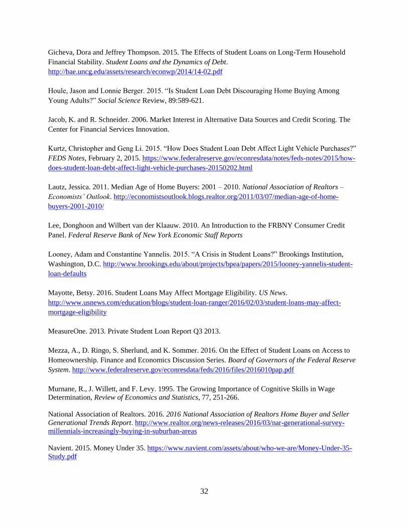
32

Gicheva, Dora and Jeffrey Thompson. 2015. The Effects of Student Loans on Long-Term Household

Financial Stability. Student Loans and the Dynamics of Debt.

http://bae.uncg.edu/assets/research/econwp/2014/14-02.pdf

Houle, Jason and Lonnie Berger. 2015. “Is Student Loan Debt Discouraging Home Buying Among

Young Adults?” Social Science Review, 89:589-621.

Jacob, K. and R. Schneider. 2006. Market Interest in Alternative Data Sources and Credit Scoring. The

Center for Financial Services Innovation.

Kurtz, Christopher and Geng Li. 2015. “How Does Student Loan Debt Affect Light Vehicle Purchases?”

FEDS Notes, February 2, 2015. https://www.federalreserve.gov/econresdata/notes/feds-notes/2015/how-

does-student-loan-debt-affect-light-vehicle-purchases-20150202.html

Lautz, Jessica. 2011. Median Age of Home Buyers: 2001 – 2010. National Association of Realtors –

Economists’ Outlook. http://economistsoutlook.blogs.realtor.org/2011/03/07/median-age-of-home-

buyers-2001-2010/

Lee, Donghoon and Wilbert van der Klaauw. 2010. An Introduction to the FRBNY Consumer Credit

Panel. Federal Reserve Bank of New York Economic Staff Reports

Looney, Adam and Constantine Yannelis. 2015. “A Crisis in Student Loans?” Brookings Institution,

Washington, D.C. http://www.brookings.edu/about/projects/bpea/papers/2015/looney-yannelis-student-

loan-defaults

Mayotte, Betsy. 2016. Student Loans May Affect Mortgage Eligibility. US News.

http://www.usnews.com/education/blogs/student-loan-ranger/2016/02/03/student-loans-may-affect-

mortgage-eligibility

MeasureOne. 2013. Private Student Loan Report Q3 2013.

Mezza, A., D. Ringo, S. Sherlund, and K. Sommer. 2016. On the Effect of Student Loans on Access to

Homeownership. Finance and Economics Discussion Series. Board of Governors of the Federal Reserve

System. http://www.federalreserve.gov/econresdata/feds/2016/files/2016010pap.pdf

Murnane, R., J. Willett, and F. Levy. 1995. The Growing Importance of Cognitive Skills in Wage

Determination, Review of Economics and Statistics, 77, 251-266.

National Association of Realtors. 2016. 2016 National Association of Realtors Home Buyer and Seller

Generational Trends Report. http://www.realtor.org/news-releases/2016/03/nar-generational-survey-

millennials-increasingly-buying-in-suburban-areas

Navient. 2015. Money Under 35. https://www.navient.com/assets/about/who-we-are/Money-Under-35-

Study.pdf

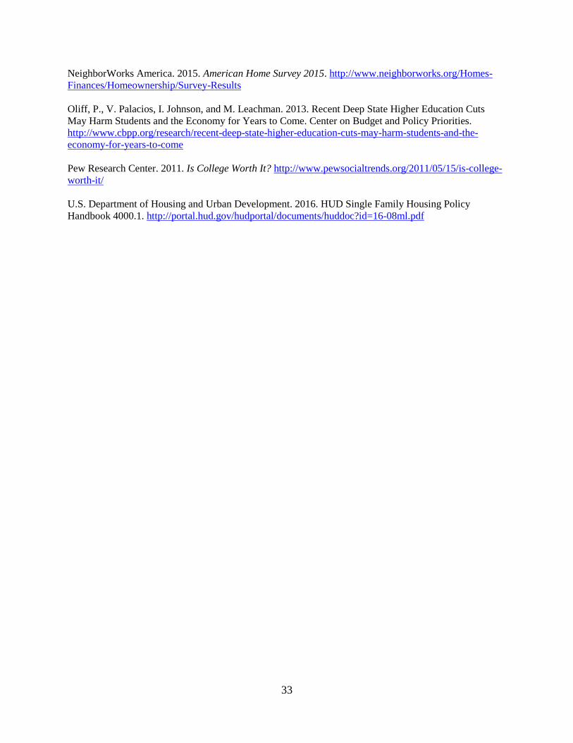
33

NeighborWorks America. 2015. American Home Survey 2015. http://www.neighborworks.org/Homes-

Finances/Homeownership/Survey-Results

Oliff, P., V. Palacios, I. Johnson, and M. Leachman. 2013. Recent Deep State Higher Education Cuts

May Harm Students and the Economy for Years to Come. Center on Budget and Policy Priorities.

http://www.cbpp.org/research/recent-deep-state-higher-education-cuts-may-harm-students-and-the-

economy-for-years-to-come

Pew Research Center. 2011. Is College Worth It? http://www.pewsocialtrends.org/2011/05/15/is-college-

worth-it/

U.S. Department of Housing and Urban Development. 2016. HUD Single Family Housing Policy

Handbook 4000.1. http://portal.hud.gov/hudportal/documents/huddoc?id=16-08ml.pdf

34

Figure 1: State enrollment-weighted mean public college & university tuition and fees, 2001-2013

Source: US Department of Education – Integrated Postsecondary Education Data System

DE, 19,836

FL, 5,010

NH, 20,241

TX, 8,129

VT, 25,231

0

5000

10000

15000

20000

25000

2000 2002 2004 2006 2008 2010 2012 2014

20

13

USD

AK AL AR AZ CA CO CT DC DE FL GA HI IA ID IL IN KS

KY LA MA MD ME MI MN MO MS MT NC ND NE NH NJ NM NV

NY OH OK OR PA RI SC SD TN TX UT VA VT WA WI WV WY

35

Figure 2: Troubled borrowers by school-leaving balance (as of 2014Q4), CCP 2009 school-leaving

cohort

0%

10%

20%

30%

40%

50%

60%

70%

1-5k 5k-10k 10k-25k 25k-50k 50k-100k 100k+

ever default ever 120+ balance higher than 2009

Source: New York Fed Consumer Credit Panel / Equifax

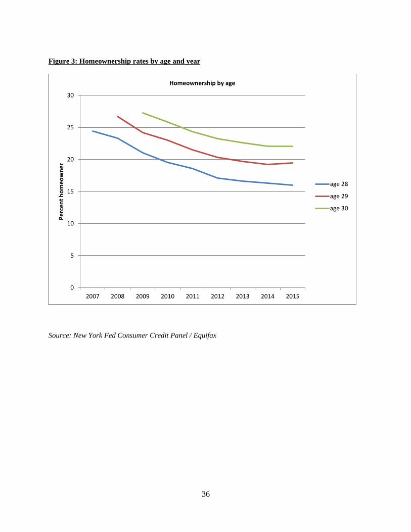
36

Figure 3: Homeownership rates by age and year

Source: New York Fed Consumer Credit Panel / Equifax

0

5

10

15

20

25

30

2007 2008 2009 2010 2011 2012 2013 2014 2015

Pe

rce

nt

ho

me

ow

ne

r

Homeownership by age

age 28

age 29

age 30

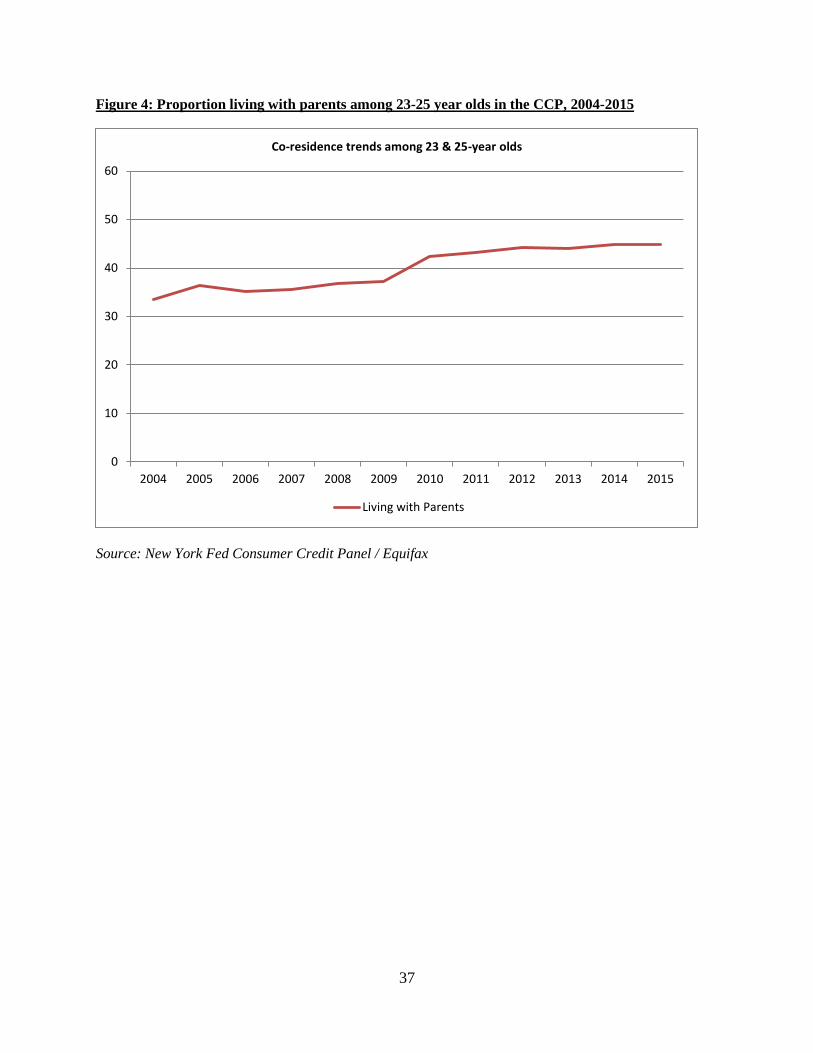
37

Figure 4: Proportion living with parents among 23-25 year olds in the CCP, 2004-2015

Source: New York Fed Consumer Credit Panel / Equifax

0

10

20

30

40

50

60

2004 2005 2006 2007 2008 2009 2010 2011 2012 2013 2014 2015

Co-residence trends among 23 & 25-year olds

Living with Parents

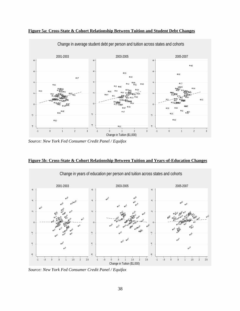
38

Figure 5a: Cross-State & Cohort Relationship Between Tuition and Student Debt Changes

Source: New York Fed Consumer Credit Panel / Equifax

Figure 5b: Cross-State & Cohort Relationship Between Tuition and Years-of-Education Changes

Source: New York Fed Consumer Credit Panel / Equifax

AK

AL

ARAZ

CA

CO

CTDC

DE

FL

GA

HI

IA

ID

IL

IN

KSKY

LA

MA

MD

ME

MI

MN

MO MS

MT

NCND

NE

NH

NJNM

NV

NY

OHOK

OR PARI

SC

SD

TNTXUT VA

VT

WA

WI

WV

WY

-4-2

02

46

8

-1 0 1 2 3

2001-2003 Change in average student debt per person ($1,000)

AK

ALARAZ

CA

CO

CT

DC

DE

FLGA

HIIA

ID

IL

IN

KS

KY

LA

MAMD

ME

MI

MN

MO

MS

MT

NC

ND

NE

NH

NJ

NMNV

NY

OH

OK

OR

PA RI

SC

SD

TN

TXUT

VA

VT

WA

WI

WV

WY

-4-2

02

46

8

-1 0 1 2 3

2003-2005

AK

AL

AR

AZ

CA

CO

CT

DC DE

FL

GA

HI

IA

ID

IL

IN

KS

KYLA

MA

MD

ME

MI

MN

MO

MS

MT

NC

ND

NE

NH

NJ

NM

NVNY

OH

OK

OR

PA

RI

SC

SD

TN

TX

UT

VA

VTWA

WI

WV

WY

-4-2

02

46

8

-1 0 1 2 3

2005-2007

Change in Tuition ($1,000)

Change in average student debt per person and tuition across states and cohorts

AL

AK

AR

AZ

CA

CO

CT

DC

DE

FL

GA

HI

IA

ID

IL

IN

KS

KY

LA

MA

MD

ME

MI

MN

MO

MS

MT

NC

ND

NE

NH

NJN

M

NV

NY

OH

OK

OR

PA

RI

SC

SD

TN

TX

UT

VA

VT

WA

WI

WV

WY

-.6

-.4

-.2

0.2

.4.6

-1 -.5 0 .5 1 1.5 2 2.5

2001-2003

AL

AK

AR A

Z

CA

CO

CT

DC

DE

FL

GA

HI

IAID

ILIN

KS

KY

LA

MA

MD

ME

MI

MN

MO

MS

MT

NC

ND

NE

NH

NJ

NM

NV

NY

OH

OK

OR

PA

RI

SC

SD

TN

TX

UT

VA

VT

WA

WI

WV

WY

-.6

-.4

-.2

0.2

.4.6

-1 -.5 0 .5 1 1.5 2 2.5

2003-2005

AL

AK

AR

AZC

A

CO

CT

DC

DE

FL

GA

HI

IA

IDIL

IN

KS K

Y

LA

MA

MD

ME

MIM

N

MO

MS M

T

NC

ND

NE

NH

NJ

NM

NV

NY

OH

OK O

R

PA

RI

SC

SD TN TX

UT

VA

VTW

A

WI

WV

WY

-.6

-.4

-.2

0.2

.4.6

-1 -.5 0 .5 1 1.5 2 2.5

2005-2007

Change in Tuition ($1,000)

Change in years of education per person and tuition across states and cohorts

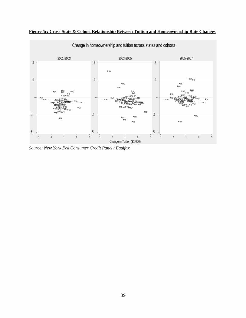
39

Figure 5c: Cross-State & Cohort Relationship Between Tuition and Homeownership Rate Changes

Source: New York Fed Consumer Credit Panel / Equifax

AK

AL

AR

AZ

CA

CO

CT

DC

DE

FLGAHI

IAID

IL

IN

KS

KY

LA

MA

MD

ME

MI

MN

MO

MS

MT

NC

ND

NE

NH

NJ

NM

NV

NYOHOK

OR

PA

RI

SC

SD

TNTX

UTVA

VT

WA

WI

WV

WY

-20

-10

010

20

-1 0 1 2 3

2001-2003

AK

AL

AR

AZ

CACO

CT

DC

DE

FLGA

HI

IA

ID

IL

IN

KS

KY

LA MA

MD

ME

MI

MN

MO

MS

MT

NC

ND

NE

NH

NJ

NM

NV

NY OH

OKOR

PA

RI

SC

SD

TN

TX

UT

VA

VTWA

WIWV

WY

-20

-10

010

20

-1 0 1 2 3

2003-2005

AK

AL

AR

AZ

CACO

CTDC

DE

FL

GAHI

IA

IDIL

IN

KS KY

LAMA

MD

ME

MI

MN

MO

MS

MT

NC

ND

NE

NHNJNM

NVNYOH

OK ORPA

RI

SC

SD

TN

TX

UT

VAVT

WAWI

WV

WY

-20

-10

010

20

-1 0 1 2 3

2005-2007

Change in Tuition ($1,000)

Change in homeownership and tuition across states and cohorts

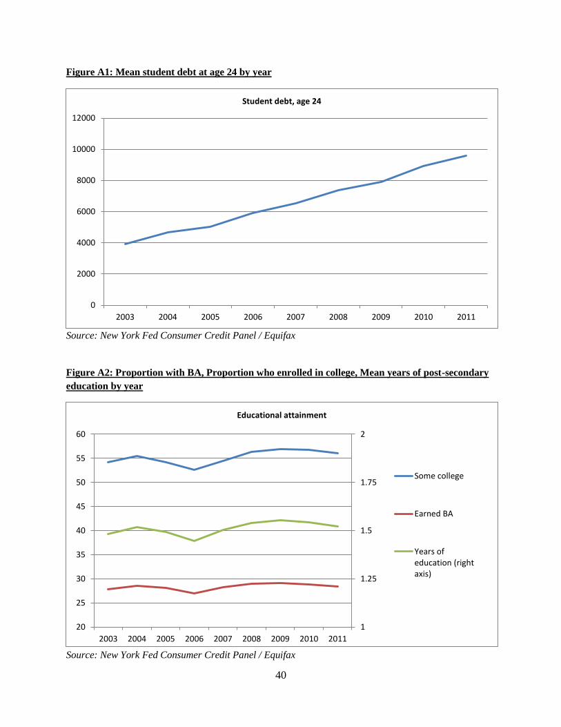
40

Figure A1: Mean student debt at age 24 by year

Source: New York Fed Consumer Credit Panel / Equifax

Figure A2: Proportion with BA, Proportion who enrolled in college, Mean years of post-secondary

education by year

Source: New York Fed Consumer Credit Panel / Equifax

0

2000

4000

6000

8000

10000

12000

2003 2004 2005 2006 2007 2008 2009 2010 2011

Student debt, age 24

1

1.25

1.5

1.75

2

20

25

30

35

40

45

50

55

60

2003 2004 2005 2006 2007 2008 2009 2010 2011

Educational attainment

Some college

Earned BA

Years ofeducation (rightaxis)

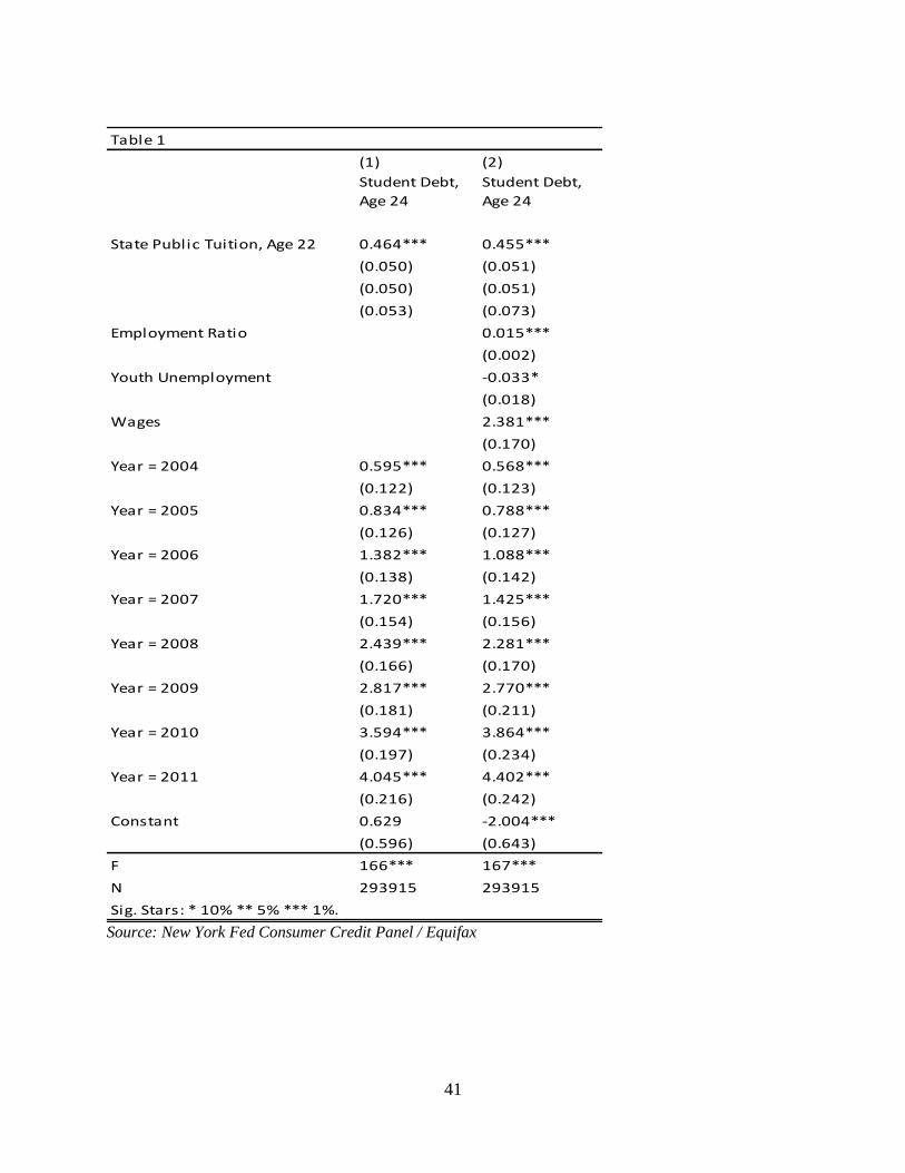
41

Source: New York Fed Consumer Credit Panel / Equifax

Table 1

(1) (2)

Student Debt,

Age 24

Student Debt,

Age 24

State Public Tuition, Age 22 0.464*** 0.455***

(0.050) (0.051)

(0.050) (0.051)

(0.053) (0.073)

Employment Ratio 0.015***

(0.002)

Youth Unemployment -0.033*

(0.018)

Wages 2.381***

(0.170)

Year = 2004 0.595*** 0.568***

(0.122) (0.123)

Year = 2005 0.834*** 0.788***

(0.126) (0.127)

Year = 2006 1.382*** 1.088***

(0.138) (0.142)

Year = 2007 1.720*** 1.425***

(0.154) (0.156)

Year = 2008 2.439*** 2.281***

(0.166) (0.170)

Year = 2009 2.817*** 2.770***

(0.181) (0.211)

Year = 2010 3.594*** 3.864***

(0.197) (0.234)

Year = 2011 4.045*** 4.402***

(0.216) (0.242)

Constant 0.629 -2.004***

(0.596) (0.643)

F 166*** 167***

N 293915 293915

Sig. Stars: * 10% ** 5% *** 1%.

42

Source: New York Fed Consumer Credit Panel / Equifax

Table 2

(1) (2) (3) (4) (5) (6)

Any college,

age 24

Any college,

age 24

Years of

education,

age 24

Years of

education,

age 24

Proportion

with BA, Age

24

Proportion

with BA, Age

24

State Public Tuition, Age 22 -0.114 -0.116 -0.008** -0.006* -0.156* -0.121

(0.099) (0.101) (0.003) (0.003) (0.089) (0.091)

(0.104) (0.115) (0.004) (0.004) (0.109) (0.106)

(0.062) (0.060) (0.002) (0.002) (0.073) (0.069)

Year = 2004 1.434** 1.365** 0.041* 0.035 0.802 0.635

(0.612) (0.620) (0.021) (0.022) (0.551) (0.558)

Year = 2005 0.532 0.496 0.026 0.016 0.488 0.204

(0.531) (0.550) (0.018) (0.019) (0.478) (0.495)

Year = 2006 -0.953* -1.002* -0.015 -0.028 -0.492 -0.866*

(0.537) (0.566) (0.019) (0.020) (0.483) (0.510)

Year = 2007 0.920* 0.849 0.045** 0.034* 0.836* 0.530

(0.549) (0.579) (0.019) (0.020) (0.495) (0.522)

Year = 2008 2.742*** 2.715*** 0.083*** 0.083*** 1.521*** 1.517***

(0.566) (0.567) (0.020) (0.020) (0.510) (0.511)

Year = 2009 3.433*** 3.437*** 0.100*** 0.116*** 1.728*** 2.214***

(0.584) (0.629) (0.020) (0.022) (0.527) (0.567)

Year = 2010 2.366*** 2.324*** 0.029 0.054* 0.228 0.980

(0.714) (0.811) (0.025) (0.028) (0.643) (0.731)

Year = 2011 1.661** 1.634** 0.004 0.024 -0.277 0.339

(0.714) (0.778) (0.025) (0.027) (0.644) (0.701)

Employment Ratio -0.008 -0.000 -0.000

(0.008) (0.000) (0.007)

Youth Unemployment -0.015 -0.005** -0.129**

(0.063) (0.002) (0.057)

Wages 0.311 -0.000 -0.094

(0.559) (0.019) (0.503)

Constant 46.502*** 47.025*** 1.079*** 1.129*** 17.873*** 19.177***

(1.802) (1.970) (0.063) (0.068) (1.623) (1.775)

F 51.5*** 49.1*** 106*** 101*** 105*** 100***

N 261181 261181 261181 261181 261181 261181

Sig. Stars: * 10% ** 5% *** 1%.

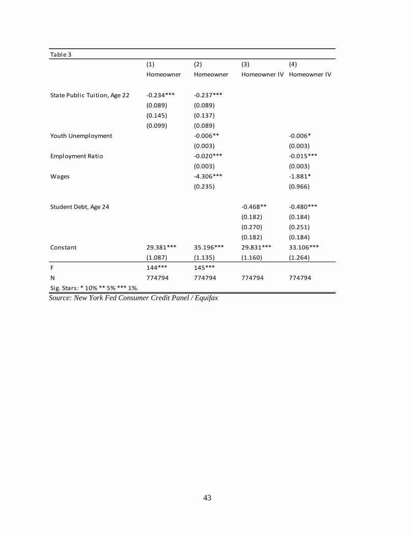
43

Source: New York Fed Consumer Credit Panel / Equifax

Table 3

(1) (2) (3) (4)

Homeowner Homeowner Homeowner IV Homeowner IV

State Public Tuition, Age 22 -0.234*** -0.237***

(0.089) (0.089)

(0.145) (0.137)

(0.099) (0.089)

Youth Unemployment -0.006** -0.006*

(0.003) (0.003)

Employment Ratio -0.020*** -0.015***

(0.003) (0.003)

Wages -4.306*** -1.881*

(0.235) (0.966)

Student Debt, Age 24 -0.468** -0.480***

(0.182) (0.184)

(0.270) (0.251)

(0.182) (0.184)

Constant 29.381*** 35.196*** 29.831*** 33.106***

(1.087) (1.135) (1.160) (1.264)

F 144*** 145***

N 774794 774794 774794 774794

Sig. Stars: * 10% ** 5% *** 1%.

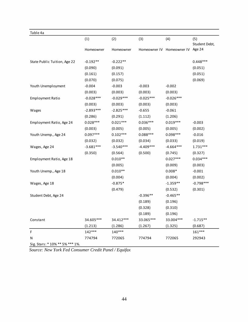
44

Source: New York Fed Consumer Credit Panel / Equifax

Table 4a

(1) (2) (3) (4) (5)

Homeowner Homeowner Homeowner IV Homeowner IV

Student Debt,

Age 24

State Public Tuition, Age 22 -0.192** -0.222** 0.448***

(0.090) (0.091) (0.051)

(0.161) (0.157) (0.051)

(0.070) (0.075) (0.069)

Youth Unemployment -0.004 -0.003 -0.003 -0.002

(0.003) (0.003) (0.003) (0.003)

Employment Ratio -0.028*** -0.029*** -0.025*** -0.026***

(0.003) (0.003) (0.003) (0.003)

Wages -2.893*** -2.825*** -0.655 -0.061

(0.286) (0.291) (1.112) (1.206)

Employment Ratio, Age 24 0.028*** 0.021*** 0.036*** 0.019*** -0.003

(0.003) (0.005) (0.005) (0.005) (0.002)

Youth Unemp., Age 24 0.097*** 0.102*** 0.088*** 0.098*** -0.016

(0.032) (0.032) (0.034) (0.033) (0.019)

Wages, Age 24 -3.681*** -3.540*** -4.409*** -4.664*** 1.731***

(0.350) (0.564) (0.500) (0.745) (0.327)

Employment Ratio, Age 18 0.010** 0.027*** 0.034***

(0.005) (0.009) (0.003)

Youth Unemp., Age 18 0.010** 0.008* -0.001

(0.004) (0.004) (0.002)

Wages, Age 18 -0.875* -1.359** -0.798***

(0.479) (0.532) (0.301)

Student Debt, Age 24 -0.396** -0.465**

(0.189) (0.196)

(0.328) (0.310)

(0.189) (0.196)

Constant 34.605*** 34.412*** 33.065*** 33.004*** -1.715**

(1.213) (1.286) (1.267) (1.325) (0.687)

F 142*** 140*** 161***

N 774794 772065 774794 772065 292943

Sig. Stars: * 10% ** 5% *** 1%.

45

Source: New York Fed Consumer Credit Panel / Equifax

Table 4b

(1) (2) (3)

Any college,

age 24

Years of

education, age

24

Proportion

with BA, age 24

State Public Tuition, Age 22 -0.124 -0.007* -0.129

(0.101) (0.004) (0.091)

(0.112) (0.004) (0.108)

(0.073) (0.002) (0.067)

Employment Ratio, Age 24 -0.010 -0.000 0.000

(0.008) (0.000) (0.007)

Youth Unemp., Age 24 -0.018 -0.005** -0.135**

(0.063) (0.002) (0.057)

Wages, Age 24 0.410 -0.002 -0.174

(0.567) (0.020) (0.511)

Wages, Age 18 0.541 0.029 0.773

(0.683) (0.024) (0.615)

Youth Unemp., Age 18 0.008 -0.000 -0.005

(0.009) (0.000) (0.008)

Employment Ratio, Age 18 -0.009 -0.000 -0.002

(0.006) (0.000) (0.006)

Constant 46.468*** 1.133*** 19.228***

(2.218) (0.077) (1.998)

F 46.9*** 95.9*** 95.7***

N 261181 261181 261181

Sig. Stars: * 10% ** 5% *** 1%.

46

Source: New York Fed Consumer Credit Panel / Equifax

Table 5

(1) (2) (3) (4) (5) (6)

Student Debt,

Age 24

Student Debt,

Age 24

Student Debt,

Age 24 Homeowner Homeowner Homeowner

State Public

Tuition, Age 22 0.375*** 0.425*** 0.412*** -0.156 -0.203** -0.178*

(0.051) (0.051) (0.051) (0.097) (0.102) (0.101)

(0.156) (0.160) (0.155) (0.157) (0.152) (0.149)

(0.050) (0.047) (0.049) (0.117) (0.174) (0.182)

Tuition * Top

Half Some

College 0.140*** -0.128**

(0.015) (0.062)

(0.094) (0.149)

(0.027) (0.050)

Tuition * Top

Half BA

Attainment 0.049*** -0.039

(0.015) (0.063)

(0.087) (0.120)

(0.016) (0.100)

Tuition * Top

Half Years of Ed 0.069*** -0.073

(0.015) (0.062)

(0.089) (0.121)

(0.009) (0.111)

Constant 0.931 0.759 0.803 29.040*** 29.255*** 29.151***

(0.597) (0.598) (0.597) (1.100) (1.106) (1.105)

F 165*** 164*** 164*** 142*** 142*** 142***

N 293915 293915 293915 774794 774794 774794

Sig. Stars: * 10% ** 5% *** 1%.

47

Source: New York Fed Consumer Credit Panel / Equifax

Table 6

(1) (2) (3) (4)

Student Debt,

Age 24

Student Debt,

Age 24 Homeowner Homeowner

State Public

Tuition * College

Attendance Rate 1.237*** -0.435***

(0.073) (0.148)

(0.303) (0.251)

(0.128) (0.130)

State Public

Tuition * Avg Yrs

of College Educ 0.417*** -0.152***

(0.020) (0.048)

(0.100) (0.083)

(0.037) (0.030)

Constant 0.536 0.906 29.145*** 28.989***

(0.587) (0.583) (1.069) (1.064)

F 170*** 172*** 144*** 144***

N 293915 293915 774794 774794

Sig. Stars: * 10% ** 5% *** 1%.

48

Source: New York Fed Consumer Credit Panel / Equifax

Table A1: Summary statistics for estimation sample

(1) (2) (3) (4) (5)

Mean Median SD Min Max

State Public Tuition, 1000s USD 6.24 5.79 2.25 2.79 20.46

Student Debt, Age 24 , 1000s USD 6.71 0 15.4 0 295.22

Youth Unemployment, CPS 11.02 10.79 3.39 2.87 21.2

Employment Ratio, QCEW 54.58 52.81 16.88 0 396.3

Wages, QCEW, 1000s USD 0.92 0.88 0.24 0 4.41

Youth Unemployment, CPS, Age 18 7.45 7.37 1.9 1.78 15.34

Employment Ratio, QCEW, Age 18 58.23 56.67 18.36 0 316.1

Wages, QCEW, Age 18, 1000s USD 0.87 0.83 0.23 0 5.38

Youth Unemployment, CPS, Age 24 9.95 9.15 3.29 2.55 20.72

Employment Ratio, QCEW, Age 24 55.77 54.72 17 0 273.26

Wages, QCEW, Age 24, 1000s USD 0.89 0.87 0.22 0 4.41

Years of Post Secondary Ed., Age 24 1.51 1 1.74 0 7

Proportion with Any College, Age 24 55.32 100 49.72 0 100

Proportion with BA, Age 24 28.35 0 45.07 0 100