Echelon Reorder Points, Installation Reorder Points, and ......the reorder point, the stage orders an integer multiple of a base quantity to bring the inventory position to above the

0025-1909/98/4412/S221$05.00Copyright q 1998, Institute for Operations Researchand the Management Sciences MANAGEMENT SCIENCE/Vol. 44, No. 12, Part 2 of 2, December 1998 S221

3b3a de02 Mp 221 Wednesday Jan 13 11:32 AM Man Sci (December, part 2) de02

Echelon Reorder Points, Installation ReorderPoints, and the Value of Centralized

Demand Information

Fangruo ChenGraduate School of Business, Columbia University, New York, New York 10027

We consider a serial inventory system with N stages. The material flows from an outsidesupplier to stage N, then to stage N0 1, etc., and finally to stage 1 where random customer

demand arises. Each stage replenishes a stage-specific inventory position according to a stage-specific reorder point/order quantity policy. Two variations of this policy are considered. Oneis based on echelon stock, and the other installation stock. The former requires centralized de-mand information, while the latter does not. The relative cost difference between the two policiesis called the value of centralized demand information. For fixed order quantities, we developefficient algorithms for computing both the optimal echelon reorder points and the optimalinstallation reorder points. These algorithms enable us to conduct an extensive computationalstudy to assess the value of centralized demand information and to understand how this valuedepends on several key system parameters, i.e., the number of stages, leadtimes, batch sizes,demand variability, and the desired level of customer service.(Supply Chain Management; Stochastic Demand; Batch Ordering; Centralized Information; ElectronicData Interchange)

1. IntroductionWe consider a serial inventory system with N stages.The material flows from an outside supplier to stage N,then to stage N 0 1, etc., and finally to stage 1, whererandom customer demand arises. Inventories are trans-ferred from one stage to the next in batches. Each stagereplenishes a stage-specific inventory position accord-ing to a stage-specific reorder point/order quantity pol-icy: whenever the inventory position falls to or underthe reorder point, the stage orders an integer multipleof a base quantity to bring the inventory position toabove the reorder point. Throughout this paper, we as-sume that the (base) order quantities are fixed and theonly decision variables are the reorder points.

We consider two variations of the reorder point/or-der quantity policy with different informational re-quirements. One is based on echelon stock: wheneverthe echelon stock at a stage falls to or below an echelon

reorder point, an order is placed. A stage’s echelon stockis the inventory position of the subsystem consisting ofthe stage itself as well as all the downstream stages. Theother variation is based on installation stock: wheneverthe installation (or local) inventory position at a stagefalls to or below an installation reorder point, an order isplaced. Note that in order to continuously monitor itsechelon stock, a stage must have access to the demandinformation at stage 1 on a real-time basis. Thus theechelon-stock policy requires centralized demand infor-mation. On the other hand, the installation-stock policyonly requires local inventory information.

A key result of this paper is that the optimal echelonreorder points can be determined sequentially: first forstage 1, then for stage 2, and so on. This is based on anobservation that the steady-state echelon inventory po-sition at each stage can be replicated by the steady-stateinventory position of a standard single-location reorder

CHENEchelon and Installation Reorder Points

S222 MANAGEMENT SCIENCE/Vol. 44, No. 12, Part 2 of 2, December 1998


point/order quantity model with a random reorder point.These random reorder points at different stages satisfya simple recursive equation that is also found in theClark-Scarf model with base-stock policies. Our result,in a nutshell, is essentially that after a proper transfor-mation, the batch-transfer model can be treated as abase-stock model for the purpose of determining theoptimal echelon reorder points.

The determination of the optimal installation reorderpoints is more difficult. We establish easy-to-computebounds on the optimal installation reorder points. Anoptimal solution can thus be found by a search. This,however, is computationally infeasible for some sys-tems, especially the ones with many stages. In response,we develop a much more efficient heuristic algorithm.It uses an empirical observation based on our numericalexperience and thus does not guarantee an optimal so-lution. However, numerical tests show that the heuristicsolution is excellent.

The above results enable us to address a fundamentalissue in supply chain management: the value of cen-tralized demand information. As mentioned earlier,echelon-stock policies require centralized demand in-formation, while installation stock policies only requirelocal information. The relative cost difference betweenthe two is a measure of the value of centralized demandinformation. In an extensive numerical study, we foundthat this value ranges from 0% to 9% with an averageof 1.75%. The numerical examples also provide insightsinto how this value depends on several parameters ofthe system, i.e., the number of stages, leadtimes, batchsizes, demand variability, and the desired level of cus-tomer service.

There is an extensive literature on serial inventorysystems. When there are no economies of scale in plac-ing orders at all the stages except the most upstreamstage, Clark and Scarf (1960) show that echelon base-stock policies are optimal in a periodic-review, finite-horizon setting. This result is later generalized toperiodic-review, infinite-horizon models by Federgruenand Zipkin (1984). Recently, Chen and Zheng (1994b)offer an exceedingly simple proof of the optimality ofthe echelon base-stock policies that also applies tocontinuous-time models. In sharp contrast, when thereare economies of scale at all stages, the optimal policiessuddenly become extremely difficult to characterize

(Clark and Scarf 1962). In fact, the optimal policies arestill unknown to this date. (Interestingly, Chen 1996characterized a heuristic policy for a two-stage, serialmodel that is guaranteed, a priori, to be within 6% ofoptimality.) As a result, research attention has been fo-cused on reasonable and easily implementable heuristicpolicies such as the reorder point/order quantity poli-cies. For this class of policies, De Bodt and Graves (1985)and Chen and Zheng (1994a) provide, respectively, anapproximate and an exact cost-evaluation procedure.An algorithm is later developed by Chen and Zheng(1998) for determining near-optimal base order quan-tities. For a comprehensive review on reorder point/order quantity policies in multiechelon, stochastic in-ventory systems, see Axsater (1993).

The value of information is a central issue in inven-tory management. It has long been recognized that de-mand information and inventory are substitutes for oneanother. For example, advanced warnings from custom-ers of their orders reduce inventory (Hariharan and Zip-kin 1995). So does the additional demand informationacquired through various marketing means (Milgromand Roberts 1988). The tradeoff between make-to-orderand make-to-stock systems also reflects the value of de-mand information (see Federgruen and Katalan (1994)and Nguyen (1995) and the references therein). Theseexamples focus on the value of better communicationbetween the customer and the supplier. Similarly, it alsocreates value to improve the communication betweensupply-chain members. The proliferation of advancedinformation technologies (e.g., EDI) in supply chainssuggests that more and more companies have come torealize the importance of better communication. Aca-demic researchers have also started to pay attention(see, e.g., Lee et al. 1997). This paper focuses on a spe-cific benefit of better communication between supplychain members: the benefit of the timely placement oforders due to the availability of echelon-stock infor-mation. (We thus ignore the other benefits such asshorter order processing times which may result frombetter communication.) As shown by Axsater and Ros-ling (1993), echelon-stock policies are superior toinstallation-stock policies in serial systems. This theo-retical result indicates that it is beneficial to have theechelon-stock information. We furnish this qualitativeobservation with extensive quantitative evidence.


MANAGEMENT SCIENCE/Vol. 44, No. 12, Part 2 of 2, December 1998 S223


The rest of the paper is organized as follows. Section2 defines the model and notation. Section 3 develops thesequential algorithm for determining the optimal eche-lon reorder points. Section 4 aims to find the optimalinstallation reorder points. Section 5 reports the com-putational study. Section 6 concludes the paper.

2. PreliminariesConsider a serial inventory system with N stages. Stage1 orders from stage 2, 2 from 3, . . . , and stage N ordersfrom an outside supplier with unlimited stock. The out-side supplier is also called stage N / 1. Each stage rep-resents a stocking point in a production system, a dis-tribution system, or a hybrid one. The production/transportation leadtimes from one stage to the next areconstant. Customers arrive at stage 1 according to aPoisson process. The demand sizes of the customers areindependent, identically distributed random variables;and they are independent of the arrival process. Thus,the demand process is compound Poisson. When stage1 runs out of stock, demand is backlogged. The systemincurs linear holding costs at every stage, and linearbackorder costs at stage 1. The objective is to minimizethe long-run average total cost in the system.

The system has the following parameters:l Å customer arrival rate,D Å demand size of a customer, a discrete random

variable, m Å E[D],Li Å leadtime from stage i / 1 to stage i, a nonnega-

tive constant,Hi Å installation holding cost rate at stage i,hi Å echelon holding cost rate at stage i Å Hi 0 Hi/1

ú 0 with HN/1 Å 0, andp Å backorder cost rate (at stage 1).

For any time epoch t, defineIi(t) Å echelon inventory at stage i

Å on-hand inventory at stage i plus inventorieson hand at, and in transit to, stages 1, . . . , i0 1,

B(t) Å backorder level at stage 1,ILi(t) Å echelon inventory level at stage i Å Ii(t)

0 B(t),IPi(t) Å echelon inventory position at stage i

Å ILi(t) plus orders in transit to stage i,ESi(t) Å echelon stock at stage i

Å IPi(t) plus outstanding orders of stage i thatare backlogged at stage i / 1, and

ISi(t) Å installation stock at stage iÅ outstanding orders at stage i (in transit to

stage i or backlogged at stage i / 1) plus on-hand inventory at stage i minus backloggedorders from stage i 0 1

Å ESi(t) 0 ESi01(t), i ¢ 2; and IS1(t) Å ES1(t).Therefore, the echelon stock at a stage changes when acustomer demand occurs at stage 1. To continuouslymonitor its echelon-stock level, a stage must have accessto the demand information at stage 1 on a real-time ba-sis. On the other hand, the installation stock at a stageis local information.

The replenishment policy is of the following type.Each stage replenishes a stage-specific inventory posi-tion according to a stage-specific (R, nQ) policy: whenthe inventory position falls to or below a reorder pointR, the stage orders a minimum integer multiple of Q(base quantity) from its upstream stage to increase theinventory position to above R. In case the upstreamstage does not have sufficient on-hand inventory to sat-isfy this order, a partial shipment is sent with the re-mainder backlogged at the upstream stage. Throughoutthis paper, we assume that the base quantities are fixedand the reorder points are the only decision variables.

Let Qi be the base quantity at stage i, i Å 1, . . . , N.We assume

Q Å n Q , i Å 1, . . . , N 0 1,i/1 i i

where ni is a positive integer. This integer-ratio con-straint simplifies analysis significantly. It also simplifiesmaterial handling (e.g., packaging and bulk breaking)by restricting the shipments to each stage to be multi-ples of a fixed quantity which may represent a truckloador the size of a standard container. Moreover, the costincrease due to the constraint is likely to be insignificantbecause inventory costs tend to be insensitive to thechoice of order quantities (Zheng (1992) and Zheng andChen (1992)).

We consider two variations of the above (R, nQ) pol-icy. One is based on echelon stock: each stage replenishesits echelon stock with an echelon reorder point. Let Ri bethe echelon reorder point at stage i, iÅ 1, . . . , N. There-fore, under an echelon-stock (R, nQ) policy, stage i or-ders a multiple of Qi from stage i / 1 every time its




echelon stock falls to or below Ri . The other variation isbased on installation stock: each stage controls its instal-lation stock with an installation reorder point. Let ri be theinstallation reorder point at stage i, iÅ 1, . . . , N. There-fore, under an installation-stock (R, nQ) policy, stage iorders a multiple of Qi from stage i / 1 every time itsinstallation stock falls to or below ri . Note that echelon-stock (R, nQ) policies require centralized demand in-formation, while installation-stock (R, nQ) policies onlyrequire local ‘demand’ information, i.e., orders from theimmediate downstream stage. When every customerdemands exactly one unit, i.e. the demand process issimple Poisson, each order by stage i is exactly of sizeQi , i Å 1, . . . , N. In this case, the (R, nQ) policy reducesto the (R, Q) policy.

We assume that the system starts with a plausible ini-tial state. That is, the initial on-hand inventory at stagei is an integer multiple of Qi01, i Å 2, . . . , N. This isreasonable because each order placed by stage i 0 1 isan integer multiple of Qi01 and thus there is no incentivefor stage i to keep a fraction of Qi01 on hand. On theother hand, every shipment to stage i is an integer mul-tiple of Qi which is itself an integer multiple of Qi01 dueto the integer-ratio constraint, and every shipment leav-ing stage i (to stage i 0 1) is an integer multiple of Qi01.This, together with the initial on-hand inventory atstage i, implies that the installation stock at stage i isalways an integer multiple of Qi01. This observation istrue whether an echelon-stock (R, nQ) policy or aninstallation-stock (R, nQ) policy is in place. Conse-quently, without any loss of generality, we restrict ri tobe an integer multiple of Qi01, i ¢ 2. Of course, r1 canbe any integer. No such restrictions are placed on Ri , iÅ 1, . . . , N.

We conclude this section with an important resultfrom Axsater and Rosling (1993). Two policies are saidto be identical if they lead to the same ordering decisions(when and how much) at every stage. Axsater and Ros-ling show that the installation-stock (R, nQ) policy, (ri ,

is identical to the echelon-stock (R, nQ) policy,NQ ) ,i iÅ1

(Ri , if and only ifNQ ) ,i iÅ1

R Å r and R Å R / Q / r , i Å 2, . . . , N. (1)1 1 i i01 i01 i

Therefore, for any installation-stock (R, nQ) policy,there exists an identical echelon-stock (R, nQ) policy;but not vice versa since ri must be an integer multiple

of Qi01 for i¢ 2. In short, installation-stock (R, nQ) pol-icies are special cases of echelon-stock (R, nQ) policies.This result is quite intuitive. Suppose the demand pro-cess is simple Poisson, and consider any installation-stock (R, Q) policy. Here orders are ‘nested’ in the sensethat every order epoch at stage i coincides with an orderepoch at stages i 0 1, i 0 2, . . . , 1. The installation stockat stage j after each order is rj / Qj for all j. Conse-quently, just before stage i places an order, its echelonstock, which is the sum of the installation stocks atstages 1 to i, is (rj / Qj) / ri . Let this echelon stocki01(jÅ1

level be Ri , i Å 1, . . . , N. It is easy to verify that theresulting echelon reorder points satisfy (1).

REMARK. As mentioned above, the paper assumesthat the base quantities have already been determinedand the only decision variables are the reorder points.The base quantities may be determined by exogenousfactors such as the size of a standard container, or theymay be a solution to a lot-sizing model. There are manylot-sizing models. Without capacity constraints, seeMuckstadt and Roundy (1993) for a serial model with-out backlogging and Chen (1998) for one with backlog-ging. With capacity constraints, see Bahl et al. (1987) fora comprehensive review of lot-sizing models. Note thatthese models all assume deterministic demands. Chenand Zheng (1998) provide a stochastic, serial model fordetermining the lot sizes.

3. Echelon Reorder PointsIn this section, we develop an efficient algorithm fordetermining the optimal echelon reorder points. The al-gorithm is based on an observation that in steady state,the echelon inventory position at each stage is essen-tially the inventory position of a standard single-stage(R, nQ) model with a random reorder point. The randomreorder points at different stages satisfy a simple recur-sive equation that is also found in the Clark-Scarf modelwith base-stock policies. As a result, the optimal echelonreorder points can be determined sequentially by solv-ing a sequence of standard single-stage problems.

We begin by reviewing some results from Chen andZheng (1994a). At time t, the systemwide holding andbackorder costs accrue at rate

N

h I (t) / pB(t).∑ i iiÅ1




Since Ii(t) Å ILi(t) / B(t) by definition, the above costrate can be written as

N

h IL (t) / (p / H )B(t).∑ i i 1iÅ1

It is convenient to introduce a time shift when assessingthe holding and backorder costs. Let li Å Lj for i ÅN(jÅi

1, . . . , N and lN/1 å 0. Thus li is the total leadtime fromthe outside supplier to stage i. At time t, we charge thefollowing cost rate:

N

h IL (t / l ) / (p / H )B(t / l ).∑ i i i 1 1iÅ1

Clearly, this shift in time does not affect the long-runaverage costs. Now suppose t is a time epoch in steadystate. Let IPi be IPi(t / li/1) and ILi be ILi(t / li), i Å 1,. . . , N. Let B Å B(t / l1). Note that B Å (IL1)0 by defi-nition, where (x)0 Å max{0, 0x}. Therefore, the long-run average system-wide cost is

NdefC(R) Å E h IL / (p / H )B∑ i i 1F G

iÅ1

where RÅ (R1, . . . , RN). The echelon reorder points thatminimize the above expression are called optimal; theyare denoted by R* Å . . . ,* *(R , R ).1 N

The distributions of IPi and ILi for i Å 1, . . . , N canbe determined recursively. Let Di be the total demandin the interval (t / li/1, t / li], i Å 1, . . . , N, which isalso referred to as the leadtime demand at stage i. Sincethe demand process is compound Poisson, Di and IPi

are independent. Moreover, D1, D2, . . . , DN are inde-pendent since the demand process has independent in-crements. The following relationship is well known:

IL Å IP 0 D , i Å 1, . . . , N. (2)i i i

From Chen and Zheng (1994a), we have

IP Å O [IL ], i Å 1, . . . , N 0 1 (3)i i i/1

where

x x ° R / Q ,i iO [x] Åi H

x 0 nQ otherwise,i

where n is the largest integer so that x 0 nQi ú Ri . (Thereason for (3) is that ILi/10 IPi is the on-hand inventory

at stage i / 1 at time t / li/1, which is always a non-negative integer multiple of Qi . For details, see Chenand Zheng (1994a).) Equations (2) and (3) provide atop-down recursive procedure for determining the dis-tributions of IPi and ILi , i Å 1, . . . , N. It is easy to seethat the distribution of IPN is uniform over {RN/ 1, . . . ,RN / QN} by simply imagining the whole system as asingle stage. (Actually, this result requires some mildregularity conditions on the demand-size distribution,see, e.g., Hadley and Whitin (1961). A sufficient condi-tion is Pr(D Å 1) ú 0. Let us make this assumption.)From (2) with i Å N, we have the distribution of ILN.From (3) with i Å N 0 1, we have the distribution ofIPN01, so on and so forth.

Now we are ready to establish new results. We firstintroduce some random variables. Define

1Pr(U Å u) Å , u Å 1, . . . , Q , i Å 1, . . . , Ni iQi

and

1Pr(Z Å z) Å , z Å 0, . . . , n 0 1, i Å 1, . . . , N 0 1.i ini

(Recall that Qi/1 Å niQi and that ni is a positive integer.)We assume that these uniform random variables are in-dependent, and they are all independent of the demandprocess.

We write X1 X2 if the two random variables X1 anddÅ

X2 have the same distribution. Clearly, X1 / X2 X1 /dÅ

X3 if X1 and X2 are independent, X1 and X3 are indepen-dent, and X2 X3. This fact will be used later.

dÅAs mentioned above, IPN is uniform over {RN / 1,

. . . , RN / QN}. Thus, IPN RN / UN. We next showdÅ

that the echelon inventory positions at the other stagescan also be decomposed in a similar fashion. (It is clearthat ESi Ri / Ui for each stage i. But for i x N, the

dÅdecomposition of IPi , which is always less than or equalto ESi , involves a random component in addition to Ui .)We begin with some intermediate results.

LEMMA 1. Ui/1 ZiQi / Ui , i Å 1, . . . , N 0 1.dÅ

PROOF. Follows from Qi/1 Å niQi . h

LEMMA 2. For i Å 1, . . . , N, Oi[X / Ui] min{Ri ,dÅ

X} / Ui , where X is any random variable independent of Ui .

PROOF. Let X Å x. Suppose x ¢ Ri . It follows fromthe definition of Oi[·] that the distribution of Oi[x/Ui]




is uniform over {Ri / 1, . . . , Ri / Qi}. Thus, Oi[x / Ui]Ri / Ui Å min{Ri , x} / Ui . Now suppose x õ Ri .

dÅAgain from the definition of Oi[·], Oi[x / Ui] Å x / Ui

Å min{Ri , x} / Ui . This completes the proof. h

We now introduce another sequence of random vari-ables. Let VN å RN. Define recursively

V Å min{R , V / Z Q 0 D },i i i/1 i i i/1

i Å 1, . . . , N 0 1. (4)

Since the U’s are independent of the demand process aswell as the Z ’s, the V ’s are independent of the U’s. Fromthe above recursive definition, it is also clear that Vi isindependent of Di for i Å 1, . . . , N and that Vi/1 is in-dependent of Zi for i Å 1, . . . , N 0 1.

THEOREM 1. IPi Vi / Ui , i Å 1, . . . , N.dÅ

PROOF. The theorem is clearly true for i Å N. Sup-pose it holds for i / 1, i.e.,

dIP Å V / U .i/1 i/1 i/1

Recall that Vi/1 and Ui/1 are independent. From Lemma1, Ui/1 ZiQi / Ui . Also recall that Vi/1 is independent

dÅof Ui and Zi , which implies that Vi/1 is independent ofZiQi / Ui . Therefore

dIP Å V / Z Q / U .i/1 i/1 i i i

Since Vi/1 is independent of Di/1 and since Zi and Ui areindependent of the demand process, the right side ofthe above equation is independent of Di/1. This, to-gether with (2) and the fact that IPi/1 is independent ofDi/1, leads to

dIL Å IP 0 D Å V / Z Q / U 0 D .i/1 i/1 i/1 i/1 i i i i/1

From (3),

IP Å O [IL ]i i i/1

dÅ O [V / Z Q 0 D / U ]i i/1 i i i/1 i

dÅ V / Ui i

where the last equality follows from Lemma 2 and thefact that Vi/1 / ZiQi 0 Di/1 is independent of Ui . Thiscompletes the induction. h

Theorem 1 indicates that IPi is precisely the steady-state inventory position of the standard single-stage (R,nQ) model with R Å Vi and Q Å Qi . A key feature here

is that the reorder point of the single-stage model is ran-dom, and it is jointly determined by the control param-eters (echelon reorder points and base quantities) atstages i, i / 1, . . . , N and the leadtime demands atstages i / 1, . . . , N. We will refer to Vi as the effectivereorder point at stage i. Consequently, the N-stage modelcan be decomposed into N single-stage (R, nQ) modelswith reorder point Vi and base quantity Qi , i Å 1, . . . ,N. The linkage between these single-stage models iscaptured by (4).

We pause here to make the following two remarks.

REMARK 1. There is a very different decompositionmethod in the multiechelon, stochastic inventory liter-ature. It is based on the observation that the actual lead-time for each order placed by a stage consists of twoparts: the production/transportation leadtime plus thedelay (or retard) experienced by the order at the up-stream stage. This delay is usually random and its char-acteristics depend on the control parameters at the up-stream stages. Therefore, one way to decompose a mul-tistage system into single-stage ones is to try tocharacterize the actual leadtimes at all stages. In contrast,our decomposition method hinges on the characteriza-tion of the effective reorder points.

REMARK 2. Equation (4) is a generalization of a sim-ilar equation found in the Clark-Scarf model with base-stock policies. This is hardly surprising since echelonbase-stock policies are special cases of echelon-stock (R,nQ) policies: an (R, nQ) policy with Q Å 1 reduces to abase-stock policy with order-up-to level SÅ R/ 1. Nowsuppose Qi Å 1, i.e., stage i follows a base-stock policywith order-up-to level Si Å Ri / 1, for i Å 1, . . . , N. Inthis case, Theorem 1 becomes IPi Vi / 1. Since ni Å 1

dÅwhich implies Zi å 0, (4) becomes

V Å min{R , V 0 D }, i Å 1, . . . , N 0 1i i i/1 i/1

with VN å RN, which is equivalent to

dIP Å min{S , IP 0 D }, i Å 1, . . . , N 0 1i i i/1 i/1

with IPN å SN. This is precisely the recursive equationfor the Clark-Scarf model (see Chen and Zheng 1994b).

With the above characterization of the steady-stateechelon inventory positions and the recursive equation(4) linking the effective reorder points, we are now




ready to develop an algorithm for identifying the opti-mal echelon reorder points.

Let us call

i

h IL / (p / H )B∑ j j 1jÅ1

the echelon cost at stage i; it includes all the holding andbackorder costs incurred in the subsystem consisting ofstages 1, . . . , i. From the recursive equations (2) and(3), we know that IPi uniquely determines the distri-butions of ILi , ILi01, . . . , IL1, and B Å (IL1)0. Given IPi

Å y, the (conditional) expected echelon cost at stage i is

idefG (y) Å E h IL / (p / H )BÉIP Å y ,∑i j j 1 iF G

jÅ1

i Å 1, . . . , N.

Since IPi Vi / Ui (Theorem 1) and only the effectivedÅ

reorder points Vi depend on the decision variables (i.e.,echelon reorder points), it is natural to express the ex-pected echelon cost at a stage as a function of its effec-tive reorder point. Define

HG (y) Å EG (y / U ), i Å 1, . . . , Ni i i

which represents the (conditional) expected echeloncost at stage i given the stage’s effective reorder point isy. Thus, the expected echelon cost at stage i is EGi(Vi).In particular,

C(R) Å E HG (V ) Å HG (R ) (5)N N N N

since VN å RN.The cost function C(R) exhibits some useful proper-

ties. Note that

N

C(R) Å h E[IL ] / EG (IP )∑ j j 1 1jÅ2

N

Å h E[IL ] / E HG (V )∑ j j 1 1jÅ2

N

Å h E[IL ] / E HG (min{R , V / Z Q 0 D }).∑ j j 1 1 2 1 1 2jÅ2

(6)

From (4), V2, . . . , VN are independent of R1. As a result,the first term in (6), hjE[ILj], is independent of R1

N(jÅ2

(see also (2) and Theorem 1). Therefore, the optimal R1

minimizes

E HG (min{R , V / Z Q 0 D }). (7)1 1 2 1 1 2

Since IL1 Å IP1 0 D1 and IP1 is independent of D1,

0G (y) Å E[h (y 0 D ) / (p / H )(y 0 D ) ]1 1 1 1 1

which is convex. Therefore, G1(·) is also convex. Let YV 1

be a finite minimum point of G1(·). Notice thatG1(min{R1, W}) is minimized at R1 Å YV 1 for any valueof W. Consequently, (7) is minimized at R1 Å YV 1. Inother words, the optimal reorder point at stage 1 is in-dependent of the reorder points at the upstream stages.Similarly, when stage 1 uses its optimal reorder point,the optimal reorder point at stage 2 is again indepen-dent of the reorder points at stages 3 to N, so on and soforth. This fact is formally established in Lemma 3 andTheorem 2 below.

Let mi Å E[Di], i Å 1, . . . , N. From the definition ofGi(·), i Å 1, . . . , N, we have from (2) and (3)

G (y) Å h (y 0 m ) / EG (IP ÉIP Å y)i/1 i/1 i/1 i i i/1

Å h (y 0 m ) / EG (O [y 0 D ]),i/1 i/1 i i i/1

i Å 1, . . . , N 0 1.

Thus, for i Å 1, . . . , N 0 1,

HG (y) Å h E(y / U 0 m )i/1 i/1 i/1 i/1

/ EG (O [y / U 0 D ])i i i/1 i/1

Lemma 1Å h E(y / U 0 m )i/1 i/1 i/1

/ EG (O [y / Z Q / U 0 D ])i i i i i i/1

Lemma 2Å h E(y / U 0 m )i/1 i/1 i/1

/ E HG (min{R , y / Z Q 0 D }). (8)i i i i i/1

The following sequence of functions are parallel to

i Å 1, . . . , N. Let GV 1(y) Å G1(y) for all y. SupposeG (·),i

GV i(·) is defined, iÅ 1, . . . , N. Let YV i be a finite minimumpoint of GV i(·). Define recursively

UG (y) Å h E(y / U 0 m )i/1 i/1 i/1 i/1

U U/ EG (min{Y , y / Z Q 0 D }),i i i i i/1

i Å 1, . . . , N 0 1. (9)




LEMMA 3. (a) GV i(·) is convex, i Å 1, . . . , N;(b) [GV i(y / 1) 0 GV i(y)] r hi (resp., 0(p / Hi/1)) as

y r /` (resp., 0`), i Å 1, . . . , N;(c) ¢ GV i(y), ∀y, i Å 1, . . . , N;HG (y)i

(d) If Rj Å YV j for j Å 1, . . . , i 0 1 then Å GV i(y),HG (y)i

∀y, i Å 1, . . . , N.

PROOF. See Appendix. h

THEOREM 2. R* Å (YV 1, YV 2, . . . , YV N) and C(R*)Å GV N(YV N).

PROOF. Take any R. From Lemma 3(c) and the def-inition of YV N, ¢ GV N(RN) ¢ GV N(YV N). Thus, fromHG (R )N N

(5), C(R) ¢ GV N(YV N). In other words, GV N(YV N) is a lowerbound on the long-run average cost of any feasibleechelon-stock (R, nQ) policy. But from Lemma 3(d),this lower bound can be achieved if R Å (YV 1, YV 2, . . . ,YV N). This completes the proof. h

Now we have an algorithm for determining the op-timal echelon reorder points. The algorithm solves Nsingle-stage (R, nQ) models sequentially. It starts atstage 1. The single-stage model for stage 1 has theholding-backorder cost function G1(·). The long-run av-erage cost of the (R1, nQ1) policy in this model is

Å The minimum point of this function,HG (R ) HG (R ).1 1 1 1

YV 1, is the optimal echelon reorder point at stage 1. Nowsuppose stage 1 uses its optimal echelon reorder point.The single-stage model for stage 2 has the holding-backorder cost function G2(·). The long-run averagecost of the (R2, nQ2) policy in this model is SinceHG (R ).2 2

R1 Å YV 1 we have from Lemma 3(d) Å GV 2(R2).HG (R )2 2

The minimum point of GV 2(·), YV 2, is the optimal echelonreorder point at stage 2. Continue in this fashion untilthe optimal echelon reorder point at stage N is found.

The above algorithm is reminiscent of the sequentialprocedure for determining the optimal base-stock levelsin the Clark-Scarf model (see Rosling (1989) and Chenand Zheng (1994b)). In fact, if Qi Å 1 for i Å 1, . . . , N,then the above algorithm reduces to the algorithm inChen and Zheng (1994b). Both algorithms determinethe optimal values of the decision variables (reorderpoints or base-stock levels) sequentially, starting at thebottom stage and ending at the top stage. For each stagei, a standard single-stage model is solved. This single-stage model assumes that all the downstream stages be-have optimally and that the immediate upstream stage

(stage i / 1) has infinite supply. The difference is thata single-stage newsboy model is solved for the Clark-Scarf model, whereas a single-stage (R, nQ) model issolved for the batch-transfer model.

4. Installation Reorder PointsAs we will see, optimal installation reorder points aremuch more difficult to find than their echelon counter-parts. In this section, we present bounds on the optimalinstallation reorder points. These bounds can then beused to search for an optimal solution. This search pro-cedure, however, is computationally infeasible for someproblem instances, especially those with many stages.In response, we develop a heuristic algorithm based ona numerical observation. Although the heuristic algo-rithm does not guarantee to find the optimal installationreorder points, numerical tests suggest that the heuristicsolution is excellent.

In §2, we mentioned that installation-stock (R, nQ)policies are special cases of echelon-stock (R, nQ) poli-cies and that the two policies are identical if and only if(1) is satisfied. Also recall that ri , the installation reorderpoint at stage i, is an integer multiple of Qi01, the basequantity at stage i 0 1, for i¢ 2. Therefore, the problemof finding the optimal installation reorder points can beformulated as:

P min C(R)

s.t. R 0 R Å m Q , m integer,i/1 i i i i

i Å 1, . . . , N 0 1.

Let R0 Å . . . , be an optimal solution to P. Let0 0(R , R )1 N

r* Å . . . , be the corresponding optimal instal-* *(r , r )1 N

lation reorder points, i.e., Å and Å 00 0 0* *r R r R R1 1 i i i01

0 Qi01 for i ¢ 2.Due to its constraints, problem P is difficult to solve.

Below, we present bounds on R0, which can be used tosearch for an optimal solution. For the sake of brevity,we only present the results informally and refer inter-ested readers to Chen (1995) for formal proofs.

We begin with bounds on Recall that GV 1(·) is con-0R .1

vex and YV 1 is its minimum point. Let yi be the ith min-imum point of GV 1(·), i Å 1, 2, . . . . Thus y1 Å YV 1. Let SÅ {y1, . . . , which is a contiguous set (see, e.g.,y },Q1

Federgruen and Zheng 1992). Let be the smallest0R1

element of S. Let Å YV 1 / Q1 0 1./R1




THEOREM 3. ° °0 0 /R R R .1 1 1

We proceed to bound Let Cf be the long-run av-0R .N

erage cost of a feasible installation-stock (R, nQ) policy.Suppose Cf is finite. Thus Cf ¢ C(R*) Å GV N(YV N) (Theo-rem 2). Define

0UR Å min{yÉG (y) ° C }N N f

and

/UR Å max{yÉG (y) ° C }.N N f

Since limyr{` GV N(y) Å /` by Lemma 3(b), both and0RN

exist and are finite./RN

THEOREM 4. ° °0 0 /R R R .N N N

Similarly, one can bound the remaining reorderpoints. Take any i Å 2, . . . , N 0 1. Imagine that the N-stage, serial system is composed of two subsystems: anupper subsystem consisting of stages i / 1, . . . , N anda lower subsystem consisting of the remaining stages.First, consider the installation holding costs incurred inthe upper subsystem. The installation inventory at stagej (¢i / 1) has two parts: the inventory on hand at stagej and the inventory in transit from stage j to stage j 0 1.Ignore the first part. Note that it takes each unit of in-ventory Lj01 units of time to travel from stage j to stagej 0 1, and that the average demand rate is lm units perunit of time, which is also the throughput rate fromstage j to stage j 0 1. By Little’s law, the average inven-tory in between stage j and stage j 0 1 is lmLj01. Sincethe installation holding cost rate is Hj at stage j, the fol-lowing is a lower bound on the long-run average hold-ing cost incurred in the upper subsystem:

N

H lmL . (10)∑ j j01jÅi/1

Now consider the lower subsystem. It is an i-stage serialsystem with an echelon holding cost rate Hi at stage i,an echelon holding cost rate hj at stage jõ i, and a back-order cost rate p. (For this truncated system, the echelonholding cost rate at stage i / 1, or the ‘‘outside sup-plier,’’ is zero.) Therefore, the holding and backordercosts in the i-stage system accrue at the following rate:

i01

H IL / h IL / (p / H )B∑i i j j 1jÅ1

i

Å H IL / h IL / (p / H )B .∑i/1 i j j 1H JjÅ1

Recall that the terms inside the curly brackets are theechelon cost at stage i, and its expected value is EGi(Vi).Since ILi Vi / Ui 0 Di , the long-run average cost in

dÅthe lower subsystem is

U

UH E(V / U 0 D ) / E HG (V ) ¢ EG (V ) (11)i/1 i i i i i i i

where

def Q / 1iU

U UG (y) Å H y / 0 m / G (y).i i/1 i iF G2

The inequality in (11) follows from Lemma 3(c).Let Cf be again the long-run average cost of a feasible

installation-stock (R, nQ) policy. Suppose it is finite. De-fine

N0

U

UR Å min yÉG (y) ° C 0 (lm) H L .∑i i f j j01H JjÅi/1

Now consider any feasible solution to P with Ri õ 0R .i

From (10) and (11), the long-run average cost of thisfeasible solution is greater than or equal to

N

U

UH lmL / EG (V ).∑ j j01 i ijÅi/1

Since Vi ° Ri õ where the first inequality follows0Ri

from (4), one can show that the above lower bound isgreater than Cf. Therefore, the considered feasible so-lution cannot be optimal.

THEOREM 5. ¢ i Å 2, . . . , N 0 1.0 0R R ,i i

The feasible region of P can be further reduced byeliminating redundant solutions. Let R Å (R1, . . . , RN)be a feasible solution to P. Suppose Ri /QiúRi/1/ Qi/1

for some i Å 1, . . . , N 0 1. Note that ILi/1(t) ° IPi/1(t)° Ri/1 / Qi/1 for any t. Therefore, ILi/1(t) õ Ri / Qi .From (3), IPi(t) Å ILi/1(t), suggesting that the on-handinventory at stage i / 1, ILi/1(t) 0 IPi(t), is always zero.As a result, the material flow from stage i / 1 to stagei is completely controlled by stage i / 1 and the up-stream stages. Now consider an alternative policy withR* Å (R1, . . . , Ri01, Ri/1, . . . , RN) where Å Ri/1R* , R*i i




/ Qi/1 0 Qi . It is easy to verify that R* is also a feasiblesolution to P. Note that under this new policy, stage i/1 still does not hold any inventory. Thus, the materialflow from stage i / 1 to stage i is still completely con-trolled by stages i/ 1, . . . , N whose control parametersare the same as before. Since the control parameters atstages 1, . . . , i 0 1 are also the same as before, the newpolicy does not change the material flow in the system.Therefore, replacing Ri with does not affect the sys-R*item performance. It is in this sense that the original so-lution R is redundant. Consequently, we can add thefollowing constraints to P:

R / Q ° R / Q , i Å 1, 2, . . . , N 0 1. (12)i i i/1 i/1

With the bounds in Theorems 3, 4 and 5 and the ad-ditional constraints in (12), one can find an optimal so-lution to P by a search. Of course, we need an initialsolution, whose long-run average cost, Cf, is needed inorder to compute the bounds. Next, we provide a heu-ristic algorithm for finding a good initial solution. Infact, as later numerical examples show, this initial so-lution is already very close to being optimal.

The heuristic algorithm is based on the following em-pirical observation. In many numerical examples, wefound that R*, the optimal echelon reorder points, con-tains useful information about r*, the optimal installa-tion reorder points. Obviously, if R* is a feasible solu-tion to P, then the problem is solved: Å and* * *r R r1 1 i

Å 0 0 Qi01 for i ¢ 2. What is interesting is* *R Ri i01

that even when R* is infeasible, one can still obtain *r ,i

i ¢ 2, by rounding 0 0 Qi01 to an integer mul-* *R Ri i01

tiple of Qi01. Formally, take any i ¢ 2. Let (resp.,0r i

be the maximum (resp., minimum) integer multiple/r )i

of Qi01 that is less (resp., larger) than or equal to *Ri

0 0 Qi01. Then, is either or Based on this0 /* *R r r r .i01 i i i

empirical observation, we restrict the installation re-order points at stages 2, . . . , N to the following set:

def0 / 0 /(r , . . . , r ) √ R Å {r , r } 1 ··· 1 {r , r }.2 N 01 2 2 N N

Note that if 0 0 Qi01 is an integer multiple of* *R Ri i01

Qi01, then Å otherwise, / Qi01Å Thus, the0 / 0 /r r ; r r .i i i i

set contains at most two points, which implies0 /{r , r }i i

that there are at most 2N01 combinations of installationreorder points in R01.

For any fixed installation reorder points at stages 2,. . . , N, it is rather easy to find the optimal reorder point

at stage 1. Take any (r2, . . . , rN) √ R01. Let r1 be thereorder point at stage 1. Let R1Å r1 and Ri Å Ri01/Qi01

/ ri for i¢ 2. Since ILj Vj/Uj0Dj and G1(·)Å GV 1(·),dÅ

we have from (6)def

C(r Ér , . . . , r ) Å C(R)1 2 N

N

UÅ h E[V / U 0 D ] / EG (V ).∑ j j j j 1 1jÅ2

Now suppose we change r1 to Å r1 / d, where d isr*1any integer. This causes every echelon reorder point toshift by d: Å Ri / d for i Å 1, . . . , N. This shift leadsR*ito a new set of effective reorder points i Å 1, . . . ,V * ,i

N. Since Å Vi / d for i Å 1, . . . , N (see (4)),V *i

C(r / dÉr , . . . , r )1 2 N

N

UÅ h E[V * / U 0 D ] / EG (V *)∑ j j j j 1 1jÅ2

N

UÅ h E[V / d / U 0 D ] / EG (V / d)∑ j j j j 1 1jÅ2

which is clearly convex in d since GV 1(·) is convex.

THEOREM 6. C(r1Ér2, . . . , rN) is convex in r1 for anyfixed installation reorder points at the upstream stages.

Here is the heuristic algorithm. First, determine 0r i

and i Å 2, . . . , N, by rounding 0 0 Qi01/ * *r , R Ri i i01

down and up to an integer multiple of Qi01. Then, foreach point in R01, find the optimal corresponding r1. Theheuristic solution is the installation reorder points thathave the lowest long-run average cost. The computa-tional complexity of this algorithm is about 2N01 timesthe effort of evaluating a single policy.

5. Numerical ExamplesThis section reports an extensive computational studydesigned to test the heuristic algorithm developed in §4for finding installation reorder points and to assess thevalue of centralized demand information.

We assume that the demand-size distribution is geo-metric, i.e.,

x01Pr(D Å x) Å (1 0 a) a, x Å 1, 2, ···

where 0 õ a ° 1. Thus E[D] Å 1/a and Var[D] Å (10 a)/a2. (Such a demand process is also referred to as




Table 1 Parameters

N 2, 3, 4, 6, 8, 10cv 1/2, 1, 2, 4p 5, 10, 15, 20L 1, 2, 3, 4m 1, 2, 3, 4

Table 2 Base Quantities

N . . . ,0 0(Q , Q )1 N

2 (8, 32)3 (8, 16, 32)4 (8, 8, 16, 32)6 (8, 8, 16, 16, 32, 32)8 (8, 8, 8, 16, 16, 16, 32, 32)

10 (8, 8, 8, 8, 16, 16, 16, 32, 32, 32)

Table 3 Performance of theHeuristic Solution

Rel. Diff. (%) No. of Examples

0 756(0, 0.5] 1(0.5, 1] 2(1, 1.5] 0(1.5, 2] 3(2, 2.5] 1(2.5, 3] 4(3, 3.5] 0(3.5, 4] 1

a stuttering Poisson process in the literature. If a Å 1then Pr(D Å 1) Å 1 and the demand process becomessimple Poisson.) Let D(1) be the total demand in oneunit of time. It can be easily verified that E[D(1)]Å l/aand Var[D(1)] Å l(2 0 a)/a2 with a coefficient of vari-ation

______√Std[D(1)] 2 0 a

cv Å Å .E[D(1)] l

The serial model is now completely specified by N,a, l, p, hi , Li , and Qi for i Å 1, . . . , N. To simplify thedesign of the computational study, we assume that 1)hi Å 1/N for i Å 1, . . . , N (thus H1 å 1), 2) Li Å L for iÅ 1, . . . , N, and 3) (Q1, . . . , QN) Å . . . ,0 0(mQ , mQ )1 N

where m is a positive integer and . . . , is fixed0 0(Q , Q )1 N

for each value of N. Table 1 summarizes the ranges ofkey parameters. The four values of cv are achieved withfour different combinations of a and l: (a, l) Å (1, 4),(1, 1), (0.4, 0.4), (0.4, 0.1). Moreover, . . . , are0 0(Q , Q )1 N

given in Table 2. There are a total of 1,536 examples.For each example, we computed the optimal echelon

reorder points by using the sequential algorithm devel-oped in §3, and the heuristic installation reorder pointsby using the heuristic algorithm developed in §4. Dueto the computational requirement of the search algo-rithm suggested in §4, we only computed the optimalinstallation reorder points for the examples with NÅ 2,3, 4 for a total of 768 examples.

To test the heuristic algorithm, we compared the av-erage cost of the heuristic solution with the average costof the optimal installation reorder points for each of the768 examples. Table 3 summarizes the results. The firstcolumn is intervals of the relative difference betweenthe two costs, i.e., (heuristic cost—optimal cost)/opti-mal cost; the second column is the corresponding num-ber of examples. The average relative difference is only0.03%. This suggests that the heuristic solution is excel-lent.

To assess the value of centralized demand informa-tion (hereafter, value of information), we compared theaverage cost of the optimal echelon reorder points withthe average cost of the optimal/heuristic installation re-order points for each of the 1,536 examples. (For theexamples with N Å 2, 3, 4, we used the average cost ofthe optimal installation reorder points. For the remain-

ing examples, we used the heuristic solution.) We de-fined the relative difference between the two costs, i.e.,(installation cost—echelon cost)/echelon cost, as ameasure of the value of information. The numerical ex-amples lead to the following observations.

(1) The value of information has a fairly wide range.The highest value is about 9%, which is achieved by anexample with N Å 6, cv Å , L Å 4, m Å 4, and p Å 20.1

2

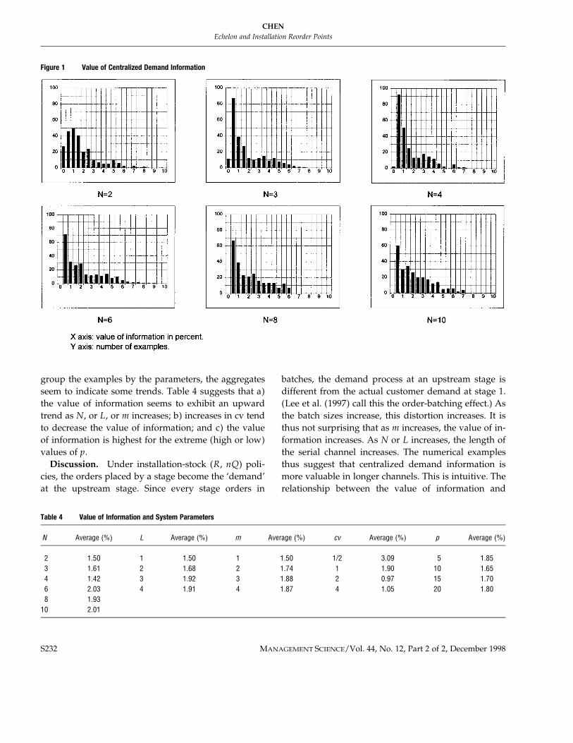
The mean is about 1.75%. Figure 1 depicts for each valueof N, the histogram of the relative cost differences.

(2) It is of interest to see how the value of informationdepends on several key parameters of the model, i.e.,N, L, m, cv, and p. Unfortunately, the individualexamples do not provide discernible patterns. But if we




Figure 1 Value of Centralized Demand Information

Table 4 Value of Information and System Parameters

N Average (%) L Average (%) m Average (%) cv Average (%) p Average (%)

2 1.50 1 1.50 1 1.50 1/2 3.09 5 1.853 1.61 2 1.68 2 1.74 1 1.90 10 1.654 1.42 3 1.92 3 1.88 2 0.97 15 1.706 2.03 4 1.91 4 1.87 4 1.05 20 1.808 1.93

10 2.01

group the examples by the parameters, the aggregatesseem to indicate some trends. Table 4 suggests that a)the value of information seems to exhibit an upwardtrend as N, or L, or m increases; b) increases in cv tendto decrease the value of information; and c) the valueof information is highest for the extreme (high or low)values of p.

Discussion. Under installation-stock (R, nQ) poli-cies, the orders placed by a stage become the ‘demand’at the upstream stage. Since every stage orders in

batches, the demand process at an upstream stage isdifferent from the actual customer demand at stage 1.(Lee et al. (1997) call this the order-batching effect.) Asthe batch sizes increase, this distortion increases. It isthus not surprising that as m increases, the value of in-formation increases. As N or L increases, the length ofthe serial channel increases. The numerical examplesthus suggest that centralized demand information ismore valuable in longer channels. This is intuitive. Therelationship between the value of information and




demand variability is surprising at first glance. Intui-tively speaking, as demand becomes more unpredicta-ble, it should be more beneficial to share the demandinformation at stage 1 with the upstream stages. Thenumerical examples suggest the reverse. One possibleexplanation is that as demand variability increases, thetotal cost increases so much that the (relative) value ofinformation actually decreases. Finally, we can interpretp as a measure of the desired level of customer service:a larger value of p signals a higher level of service. Asp increases, it becomes more important to replenish in-ventories in a timely fashion and thus the value of in-formation should increase. Then, why is the value ofinformation so high when p Å 5? The reason might be,again, that a small value of p leads to a lower total cost,resulting in an increase in the (relative) value of infor-mation.

Note. We implicitly assumed above that both theechelon-stock policy and the installation-stock policyuse the same base quantities. This assumption is cer-tainly valid if the base quantities are not decision vari-ables, i.e. they are determined by exogenous factors.Otherwise, the two policies may call for different basequantities. In this case, the above assessment of thevalue of information is approximate. But it is reasonableto believe that the approximation is good since inven-tory costs tend to be insensitive to the choice of basequantities (Zheng and Chen 1992). Finally, it is inter-esting to note that the above findings are similar to thosefound by Krajewski et al. (1987) in a large scale simu-lation study of complex manufacturing environments.

6. Closing RemarksThis paper studies the reorder point/order quantitypolicy, or the (R, nQ) policy, in serial inventory systems.A key finding is that a serial system with N stages canbe decomposed into N single-stage systems, each witha random reorder point. This observation leads to effi-cient algorithms for determining both the optimal ech-elon reorder points and the optimal installation reorderpoints. Although the paper confines itself tocontinuous-time models with compound Poisson de-mand processes, it is straightforward to extend all theresults to discrete-time models with independent andidentically distributed demands.

The paper has provided the first extensive numericalevidence on the value of centralized demand informa-tion, which is defined to be the relative cost differencebetween echelon-stock and installation-stock policies.(Echelon-stock policies use centralized demand infor-mation, while installation-stock policies use only localinformation.) In a pool of 1,536 examples, it is foundthat the value of information has a fairly wide rangewith the highest value of 9% and a mean of 1.75%. Thenumerical examples also suggest that the value of in-formation tends to increase as a result of increases inthe number of stages, the leadtimes, or the batch sizes.Interestingly, higher demand variability decreases thevalue of information, and extreme levels of customerservice (either high or low) tend to increase the value.1

1 The author would like to thank Paul Zipkin, an Associate Editor andtwo referees for their helpful comments on a previous version of thispaper.

AppendixPROOF OF LEMMA 3. (a) Recall that G1(y) Å E[h1(y 0 D1) / (p

/ H1)(y 0 D1)0]. Thus G1(·) is convex, implying that G1(·) is convex.Since GV 1(y) Å G1(y) by definition, Lemma 3(a) holds for i Å 1. Nowsuppose GV i(·) is convex. Thus GV i(min{YV i , y}) is convex in y. This, to-gether with (9), implies that GV i/1(·) is convex. This completes the in-duction.

(b) Let (x)/ Å max{0, x}. Since x / (x)0 Å (x)/, G1(y) Å E[h1(y0 D1)/ / (p / H2)(y 0 D1)0]. It is then clear that [G1(y / 1)0 G1(y)] r h1 (resp., 0(p / H2)) as y r /` (resp., 0`). From thedefinition of GV 1(·), Lemma 3(b) holds for i Å 1. Now suppose it holdsfor i. To show that the lemma holds for i / 1, note that the inductionassumption implies that EGV i(min{YV i , y / ZiQi 0 Di/1}) as a functionof y becomes flat as y r/` and becomes linear with slope0(p/Hi/1)as y r 0`. Thus, from (9)

U Ulim [G (y / 1) 0 G (y)] Å h / 0 Å hi/1 i/1 i/1 i/1yr/`

and

U Ulim [G (y / 1) 0 G (y)] Å h 0 (p / H ) Å 0(p / H ).i/1 i/1 i/1 i/1 i/2yr0`

This completes the induction.(c) By definition, Lemma 3(c) holds (with equality) for i Å 1. Now

suppose it holds for i. Thus, for any W,

U U U

HG (min{R , W}) ¢ G (min{R , W}) ¢ G (min{Y , W}). (13)i i i i i i

From (8),(13)

HG (y) ¢ h E(y / U 0 m )i/1 i/1 i/1 i/1

U U U/ EG (min{Y , y / Z Q 0 D }) Å G (y). (14)i i i i i/1 i/1

Thus Lemma 3(c) holds for i / 1. This completes the induction.




(d) Lemma 3(d) clearly holds for i Å 1. Now suppose it holds fori. Suppose Rj Å YV j for j Å 1, . . . , i. By the induction assumption, Gi(y)Å GV i(y) for all y. This, together with Ri Å YV i , implies that the twoinequalities in (13) now hold as equalities. As a result, the inequalityin (14) becomes an equality. This completes the induction. h

ReferencesAxsater, S. 1993. Continuous Review Policies for Multi-Level Inven-

tory Systems with Stochastic Demand,’’ in Handbook in OperationsResearch and Management Science, Vol. 4, Logistics of Production andInventory, S. Graves, A. Rinnooy Kan and P. Zipkin, eds. North-Holland, Amsterdam, 1993., K. Rosling. 1993. Installation vs. echelon stock policies for multi-level inventory control. Management Sci. 39 1274–1280.

Bahl, H., L. Ritzman, J. Gupta. 1987. Determining lot sizes and resourcerequirements: a review. Oper. Res. 35 329–345.. 1995. Echelon reorder points, installation reorder points, and thevalue of centralized demand information. Unabridged WorkingPaper, Graduate School of Business, Columbia University, NewYork.. 1996. 94%-Effective policies for a two-stage serial system withstochastic demand. Working Paper, Graduate School of Business,Columbia University, New York.

Chen, F. 1998. Stationary policies in multi-echelon inventory systemswith deterministic demand and backlogging. Oper. Res. 46 S26–S34., Y.-S. Zheng. 1994a. Evaluating echelon stock (R, nQ) policies inserial production/inventory systems with stochastic demand.Management Sci. 40 1262–1275., . 1994b. Lower bounds for multi-echelon stochastic inven-tory systems. Management Sci. 40 1426–1443., . 1998. Near-optimal echelon-stock (R, nQ) policies in multi-stage serial systems. Oper. Res. 46 592–602.

Clark, A., H. Scarf. 1960. Optimal policies for a multi-echelon inven-tory problem. Management Sci. 6 475–490., . 1962. Approximate solutions to a simple multi-echelon in-ventory problem. K. Arrow, S. Karlin and H. Scarf eds., Studies in

Applied Probability and Management Science, Stanford UniversityPress, Stanford, CA.

De Bodt, M., S. Graves. 1985. Continuous review policies for a multi-echelon inventory problem with stochastic demand. ManagementSci. 31 1286–1295.

Federgruen, A., Z. Katalan. 1994. Make-to-stock or make-to-order: thatis the question; Novel Answers to an Ancient Debate. GraduateSchool of Business, Columbia University, New York, 1994., Y.-S. Zheng. 1992. An efficient algorithm for computing an op-timal (r, Q) policy in continuous review stochastic inventory sys-tems. Oper. Res. 40 808–813., P. Zipkin. 1984. Computational issues in an infinite-horizon,multi-echelon inventory model. Oper. Res. 32 818–836.

Hadley, G., T. Whitin. 1961. A family of inventory models. ManagementSci. 7 351–371.

Hariharan, R., P. Zipkin. 1995. Customer-order information, leadtimes,and inventories. Management Sci. 41 1599–1607.

Krajewski, L., B. King, L. Ritzman, D. Wong. 1987. Kanban, MRP, andshaping the manufacturing environment. Management Sci. 33 39–57.

Lee, H., P. Padmanabhan, S. Whang. 1997. Information distortion in asupply chain: the bullwhip effect. Management Sci. 43 546–558.

Milgrom, P., J. Roberts. 1988. Communication and inventory as sub-stitutes in organizing production. Scand. J. Econom. 90 275–289.

Muckstadt, J., R. Roundy, 1993. Analysis of multi-stage productionsystems. S. Graves, A. Rinnooy Kan and P. Zipkin, eds., Handbookin Operations Research and Management Science, Vol. 4, Logistics ofProduction and Inventory, North-Holland, Amsterdam.

Nguyen, V. 1995. On base-stock policies for make-to-order/make-to-stock production. MIT, Cambridge, MA.

Rosling, K. 1989. Optimal inventory policies for assembly systems un-der random demand. Oper. Res. 37 565–579.

Zheng, Y.-S. 1992. On properties of stochastic inventory systems. Man-agement Sci. 38 87–103., F. Chen. 1992. Inventory policies with quantized ordering. NavalRes. Logist. 39 285–305.

Accepted by Hau L. Lee; received March 19, 1996. This paper has been with the author 7 months for 2 revisions.

Documents

Echelon Reorder Points, Installation Reorder Points, and ......the reorder point, the stage orders an integer multiple of a base quantity to bring the inventory position to above the