ECEN5533 Modern Communications TheoryLecture #1 19 August 2014Dr. George Scheetswww.okstate.edu/elec-engr/scheets/ecen5533

ECEN5533 Modern Communications TheoryLecture #1 19 August 2014Dr. George Scheetswww.okstate.edu/elec-engr/scheets/ecen5533

Review Chapter 1.1 - 1.4Review Chapter 1.1 - 1.4Problems: 1.1a-c, 1.4, 1.5, 1.9Problems: 1.1a-c, 1.4, 1.5, 1.9

ECEN5533 Modern Communications TheoryLecture #2 21 August 2014Dr. George Scheets

ECEN5533 Modern Communications TheoryLecture #2 21 August 2014Dr. George Scheets

Review Chapter 1.5 - 1.8Review Chapter 1.5 - 1.8Problems: 1.13 - 1.16, 1.20Problems: 1.13 - 1.16, 1.20

Quiz #1Quiz #1 Local: Tuesday, 4 September, Lecture 6Local: Tuesday, 4 September, Lecture 6 Off Campus DL: Off Campus DL: << 11 September 11 September

ECEN5533 Modern Communications TheoryLecture #3 26 August 2014Dr. George Scheets

ECEN5533 Modern Communications TheoryLecture #3 26 August 2014Dr. George Scheets

Review Appendix AReview Appendix AProblems: Quiz #1, 2011-2013Problems: Quiz #1, 2011-2013

Quiz #1Quiz #1 Local: Thursday, 4 September, Lecture 6Local: Thursday, 4 September, Lecture 6 Off Campus DL: Off Campus DL: << 11 September 11 September

ECEN5533 Modern Communications TheoryLecture #4 28 August 2014

ECEN5533 Modern Communications TheoryLecture #4 28 August 2014

Read: 5.1 - 5.3Read: 5.1 - 5.3 Problems: 5.1 - 5.3Problems: 5.1 - 5.3 Quiz #1Quiz #1

Local: Thursday, 4 September, Lecture 6Local: Thursday, 4 September, Lecture 6 Off Campus DL: Off Campus DL: << 11 September 11 September

www.okstate.edu/elec-engr/scheets/ecen5533/www.okstate.edu/elec-engr/scheets/ecen5533/

ECEN5533 Modern Communications TheoryLecture #5 2 September 2014Dr. George Scheets

ECEN5533 Modern Communications TheoryLecture #5 2 September 2014Dr. George Scheets Read 5.4 & 5.5Read 5.4 & 5.5 Problems 5.7 & 5.12Problems 5.7 & 5.12 Quiz #1Quiz #1

Local: Local: Thursday, 4 SeptemberThursday, 4 September, Lecture 6, Lecture 6 Off Campus DL: Off Campus DL: << 11 September 11 September Strictly Review (Chapter 1)Strictly Review (Chapter 1)

Full Period, Open Book & NotesFull Period, Open Book & Notes

GradingGrading In Class: 2 Quizzes, 2 Tests, 1 Final ExamIn Class: 2 Quizzes, 2 Tests, 1 Final Exam

Open Book & Open NotesOpen Book & Open NotesWARNING! WARNING! Study for them like they’re closed book!Study for them like they’re closed book!

Graded Homework: 2 Design ProblemsGraded Homework: 2 Design Problems Ungraded Homework: Ungraded Homework:

Assigned most every classAssigned most every classNot collectedNot collectedSolutions ProvidedSolutions ProvidedPayoff: Tests & QuizzesPayoff: Tests & Quizzes

Why work the ungraded Homework problems?Why work the ungraded Homework problems? An Analogy: Commo Theory vs. FootballAn Analogy: Commo Theory vs. Football Reading the text = Reading a playbookReading the text = Reading a playbook WorkingWorking the problems = the problems =

playing in a scrimmage playing in a scrimmage Looking at the problem solutions = Looking at the problem solutions =

watching a scrimmage watching a scrimmage Quiz = Exhibition GameQuiz = Exhibition Game Test = Big GameTest = Big Game

To succeed in this class...To succeed in this class...

Show some self-discipline!! Important!!Show some self-discipline!! Important!!For every hour of class...For every hour of class...

... put in 1-2 hours of your own effort.... put in 1-2 hours of your own effort.

PROFESSOR'S LAMENTPROFESSOR'S LAMENTIf you put in the timeIf you put in the timeYou should do fine.You should do fine.If you don't,If you don't,You likely won't.You likely won't.

Course EmphasisCourse Emphasis

DigitalDigital AnalogAnalog

Binary Binary M-aryM-ary

Wide BandWide Band Narrow BandNarrow Band

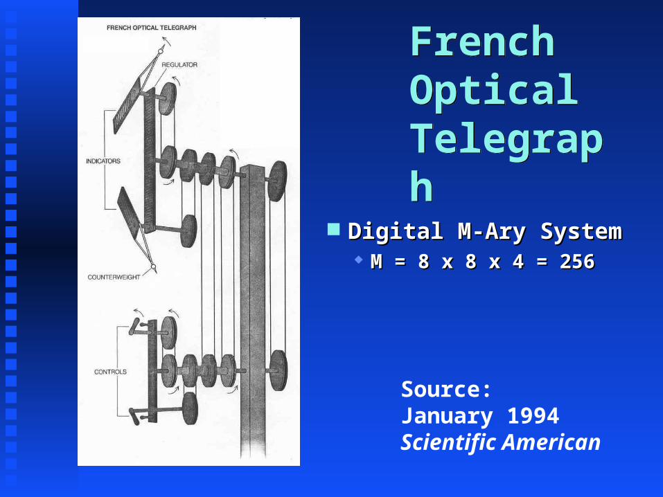
French Optical Telegraph

French Optical Telegraph

Source:January 1994Scientific American

Digital M-Ary SystemDigital M-Ary System M = 8 x 8 x 4 = 256M = 8 x 8 x 4 = 256

French System MapFrench System Map

Source: January 1994Scientific American

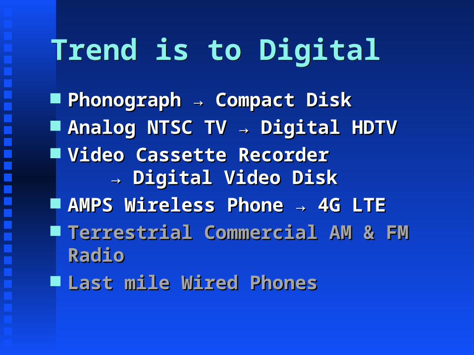
Trend is to DigitalTrend is to Digital

Phonograph → Compact DiskPhonograph → Compact Disk Analog NTSC TV → Digital HDTVAnalog NTSC TV → Digital HDTV Video Cassette Recorder Video Cassette Recorder

→ Digital Video Disk→ Digital Video Disk AMPS Wireless Phone → 4G LTEAMPS Wireless Phone → 4G LTE Terrestrial Commercial AM & FM RadioTerrestrial Commercial AM & FM Radio Last mile Wired PhonesLast mile Wired Phones

Review...Review...

Fourier Transforms X(f)Fourier Transforms X(f)Table 2-4 & 2-5Table 2-4 & 2-5

Power SpectrumPower SpectrumGiven X(f) Given X(f)

Power SpectrumPower SpectrumUsing AutocorrelationUsing Autocorrelation Use Time Average AutocorrelationUse Time Average Autocorrelation

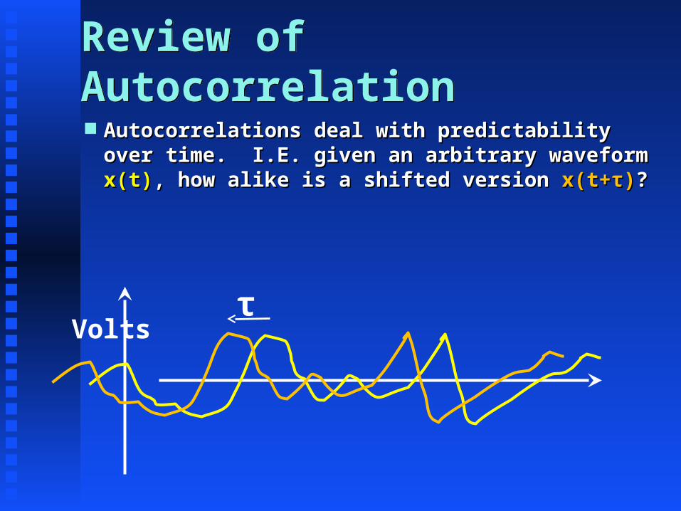
Review of AutocorrelationReview of Autocorrelation

Autocorrelations deal with predictability over time. I.E. Autocorrelations deal with predictability over time. I.E. given an arbitrary point given an arbitrary point x(t1)x(t1), how predictable is , how predictable is x(t1+tau)x(t1+tau)??

time

Volts

t1

tau

Review of AutocorrelationReview of Autocorrelation

Autocorrelations deal with predictability over time. I.E. Autocorrelations deal with predictability over time. I.E. given an arbitrary waveform given an arbitrary waveform x(t)x(t), how alike is a shifted , how alike is a shifted version version x(t+x(t+ττ))??

Voltsτ

255 point discrete time White Noise waveform

(Adjacent points are independent)

255 point discrete time White Noise waveform

(Adjacent points are independent)

time

Volts

0

Vdc = 0 v, Normalized Power = 1 watt

If true continuous time White Noise, no predictability.

Rxx(0)Rxx(0)

The sequence x(n)The sequence x(n)x(1) x(2) x(3) ... x(255)x(1) x(2) x(3) ... x(255)

multiply it by the unshifted sequence x(n+0)multiply it by the unshifted sequence x(n+0)x(1) x(2) x(3) ... x(255)x(1) x(2) x(3) ... x(255)

to get the squared sequenceto get the squared sequencex(1)x(1)22 x(2) x(2)22 x(3) x(3)22 ... x(255) ... x(255)22

Then take the time averageThen take the time average[x(1)[x(1)22 +x(2) +x(2)22 +x(3) +x(3)22 ... +x(255) ... +x(255)22]/255]/255

Rxx(1)Rxx(1)

The sequence x(n)The sequence x(n)x(1) x(2) x(3) ... x(254) x(255)x(1) x(2) x(3) ... x(254) x(255)

multiply it by the shifted sequence x(n+1)multiply it by the shifted sequence x(n+1)x(2) x(3) x(4) ... x(255)x(2) x(3) x(4) ... x(255)

to get the sequenceto get the sequencex(1)x(2) x(2)x(3) x(3)x(4) ... x(254)x(255)x(1)x(2) x(2)x(3) x(3)x(4) ... x(254)x(255)

Then take the time averageThen take the time average[x(1)x(2) +x(2)x(3) +... +x(254)x(255)]/254[x(1)x(2) +x(2)x(3) +... +x(254)x(255)]/254

Review of AutocorrelationReview of Autocorrelation

If the average is positive...If the average is positive... Then x(t) and x(t+tau) tend to be alikeThen x(t) and x(t+tau) tend to be alike

Both positive or both negativeBoth positive or both negative If the average is negativeIf the average is negative

Then x(t) and x(t+tau) tend to be oppositesThen x(t) and x(t+tau) tend to be oppositesIf one is positive the other tends to be negativeIf one is positive the other tends to be negative

If the average is zeroIf the average is zero There is no predictabilityThere is no predictability

Autocorrelation Estimate of Discrete Time White NoiseAutocorrelation Estimate of Discrete Time White Noise

tau (samples)

Rxx

0

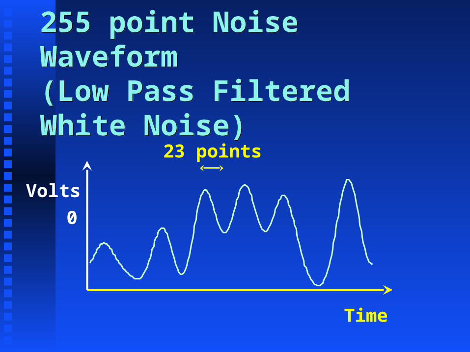
255 point Noise Waveform(Low Pass Filtered White Noise)255 point Noise Waveform(Low Pass Filtered White Noise)

Time

Volts

23 points

0

Autocorrelation Estimate of Low Pass Filtered White NoiseAutocorrelation Estimate of Low Pass Filtered White Noise

tau samples

Rxx

0

23

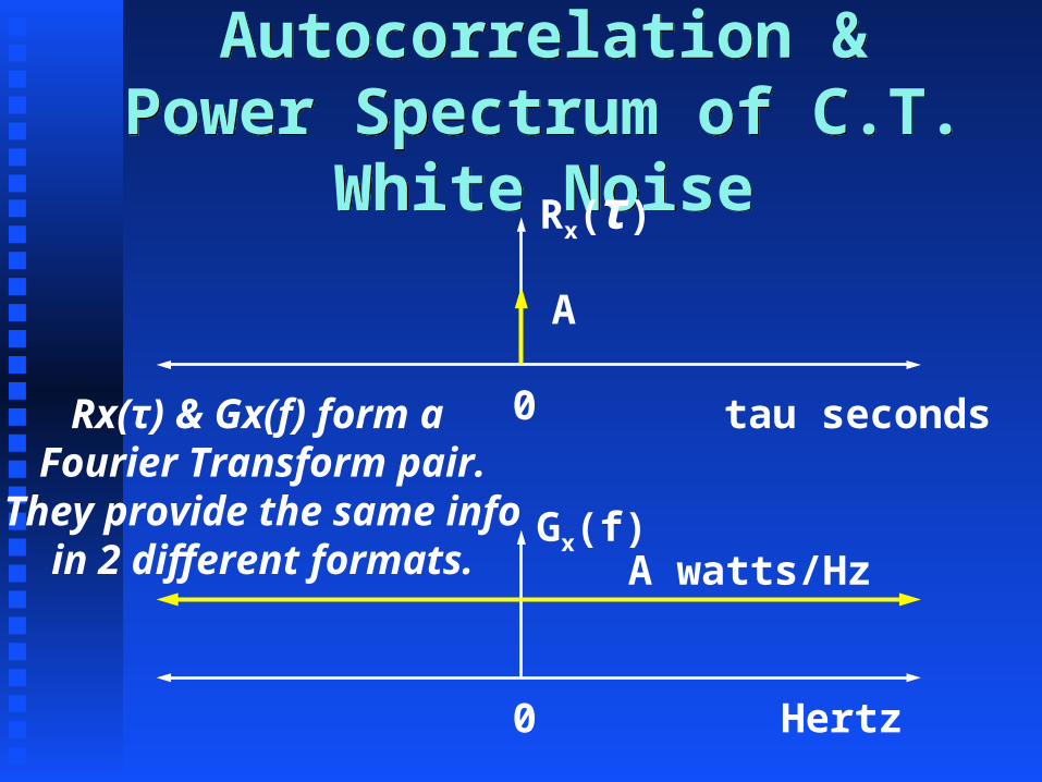
Autocorrelation & Power Spectrum of C.T. White Noise

Autocorrelation & Power Spectrum of C.T. White Noise

Rx(τ)

tau seconds0

A

Gx(f)

Hertz0

A watts/Hz

Rx(τ) & Gx(f) form a Fourier Transform pair.

They provide the same infoin 2 different formats.

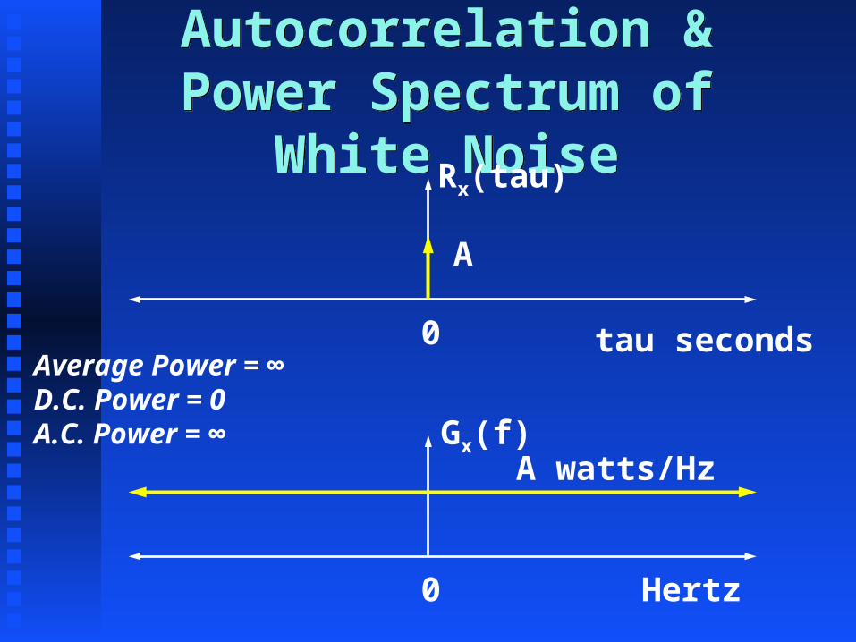
Autocorrelation & Power Spectrum of White NoiseAutocorrelation & Power Spectrum of White Noise

Rx(tau)

tau seconds0

A

Gx(f)

Hertz0

A watts/Hz

Average Power = ∞D.C. Power = 0A.C. Power = ∞

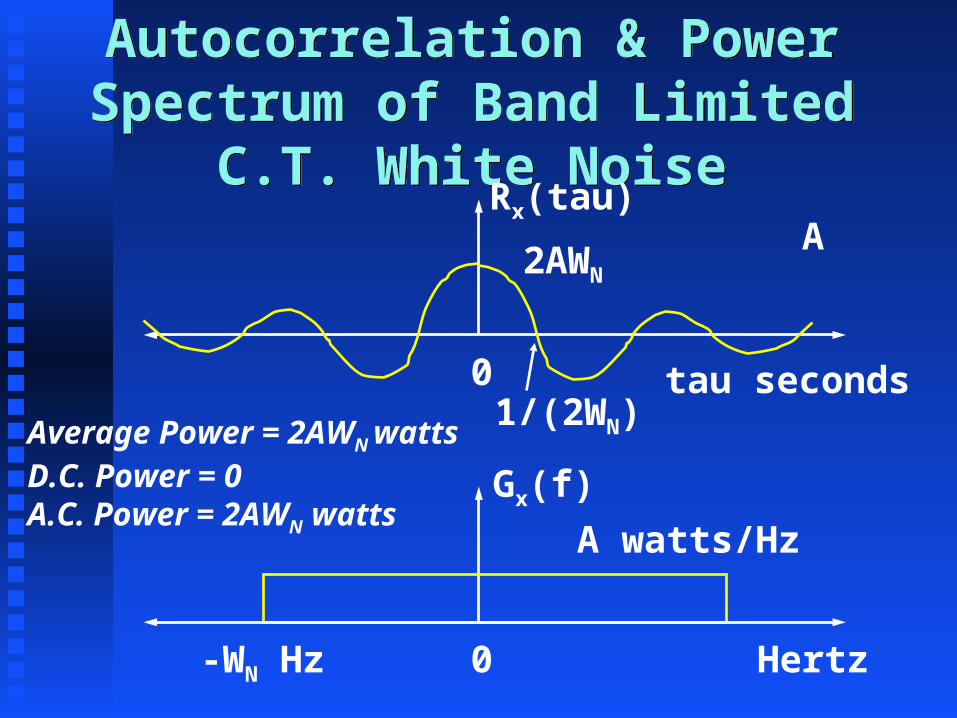
Autocorrelation & Power Spectrum of Band Limited C.T. White Noise

Autocorrelation & Power Spectrum of Band Limited C.T. White Noise

Rx(tau)

tau seconds0

A

Gx(f)

Hertz0

A watts/Hz

-WN Hz

2AWN

1/(2WN)Average Power = 2AWN wattsD.C. Power = 0A.C. Power = 2AWN watts

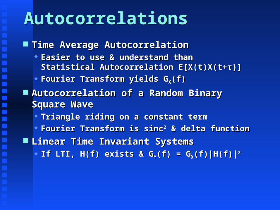
AutocorrelationsAutocorrelations Time Average AutocorrelationTime Average Autocorrelation

Easier to use & understand than Easier to use & understand than Statistical Autocorrelation E[X(t)X(t+Statistical Autocorrelation E[X(t)X(t+ττ)])]

Fourier Transform yields GFourier Transform yields GXX(f)(f)

Autocorrelation of a Random Binary Square WaveAutocorrelation of a Random Binary Square Wave Triangle riding on a constant termTriangle riding on a constant term Fourier Transform is sincFourier Transform is sinc22 & delta function & delta function

Linear Time Invariant SystemsLinear Time Invariant Systems If LTI, H(f) exists & GIf LTI, H(f) exists & GYY(f) = G(f) = GXX(f)|H(f)|(f)|H(f)|22

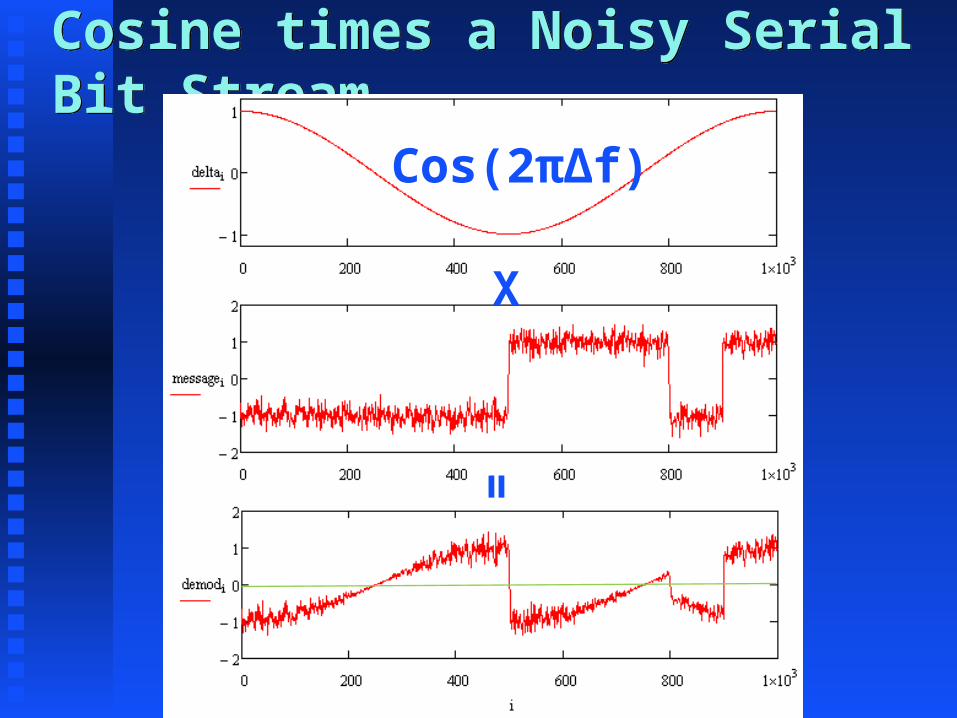
Cosine times a Noisy Serial Bit StreamCosine times a Noisy Serial Bit Stream

X

=

Cos(2πΔf)

LTILTI

If input is x(t) = Acos(ωt)output must be of form

y(t) = Bcos(ωt+θ)

Filterx(t) y(t)

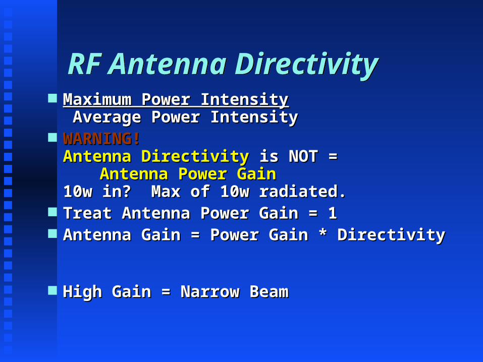
RF Antenna DirectivityRF Antenna Directivity Maximum Power IntensityMaximum Power Intensity

Average Power Intensity Average Power Intensity WARNING!WARNING!

Antenna DirectivityAntenna Directivity is NOT = is NOT = Antenna Power GainAntenna Power Gain

10w in? Max of 10w radiated.10w in? Max of 10w radiated. Treat Antenna Power Gain = 1Treat Antenna Power Gain = 1 Antenna Gain = Power Gain * Directivity Antenna Gain = Power Gain * Directivity

High Gain = Narrow BeamHigh Gain = Narrow Beam

Directional AntennasDirectional Antennas

RF Antenna Gain RF Antenna Gain

Antenna Gain is what goes in RF Link Antenna Gain is what goes in RF Link EquationsEquations

In this class, unless specified otherwise, In this class, unless specified otherwise, assume antennas are properly aimed.assume antennas are properly aimed. Problems specify peak antenna gainProblems specify peak antenna gain

High Gain Antenna = Narrow BeamHigh Gain Antenna = Narrow Beam

Parabolic DirectivityParabolic Directivity s

ourc

e: e

n.w

ikip

edia

.org

/wik

i/P

arab

olic

_an

ten

na

Effective Isotrophic Radiated Power

Effective Isotrophic Radiated Power

EIRP = PEIRP = PttGGtt

Path Loss LPath Loss Ls s = (4*= (4*ππ*d/*d/λλ))22

Link AnalysisLink Analysis

Final Form of Analog Free Space Final Form of Analog Free Space RF Link EquationRF Link EquationPPrr = EIRP*G = EIRP*Grr/(L/(Lss*M*L*M*Loo) ) (watts)(watts)

Derived Digital Link EquationDerived Digital Link EquationEEbb//NNoo = EIRP*G = EIRP*Grr/(R*k*T*L/(R*k*T*Lss*M*Lo)*M*Lo)

(dimensionless)(dimensionless)

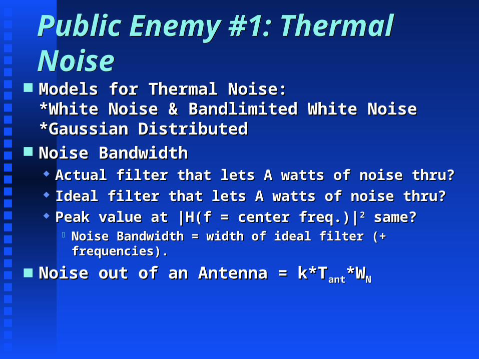
Public Enemy #1: Thermal NoisePublic Enemy #1: Thermal Noise Models for Thermal Noise: Models for Thermal Noise:

*White Noise & Bandlimited White Noise*White Noise & Bandlimited White Noise*Gaussian Distributed*Gaussian Distributed

Noise BandwidthNoise Bandwidth Actual filter that lets A watts of noise thru?Actual filter that lets A watts of noise thru? Ideal filter that lets A watts of noise thru?Ideal filter that lets A watts of noise thru? Peak value at |H(f = center freq.)|Peak value at |H(f = center freq.)|22 same? same?

Noise Bandwidth = width of ideal filter (+ frequencies).Noise Bandwidth = width of ideal filter (+ frequencies).

Noise out of an Antenna = k*TNoise out of an Antenna = k*Tantant*W*WNN

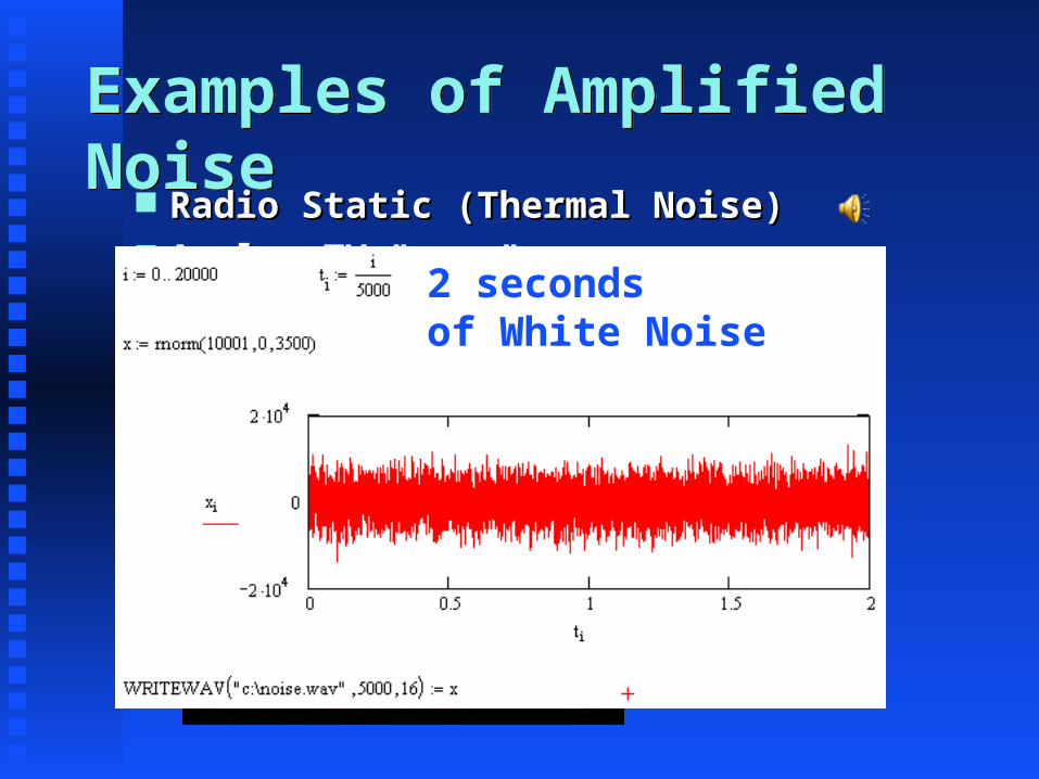
Examples of Amplified NoiseExamples of Amplified Noise Radio Static (Thermal Noise)Radio Static (Thermal Noise) Analog TV "snow"Analog TV "snow"2 seconds

of White Noise

Review of PDF's & HistogramsReview of PDF's & Histograms Probability Density Functions (PDF's), of which a Probability Density Functions (PDF's), of which a

Histograms is an estimate of shape, frequently (but not Histograms is an estimate of shape, frequently (but not always!) deal with the voltage likelihoods always!) deal with the voltage likelihoods

Time

Volts

255 point discrete time White Noise waveform

(Adjacent points are independent)

255 point discrete time White Noise waveform

(Adjacent points are independent)

time

Volts

0

Vdc = 0 v, Normalized Power = 1 watt

If true continuous time White Noise, No Predictability.

15 Bin Histogram(255 points of Uniform Noise)15 Bin Histogram(255 points of Uniform Noise)

Volts

BinCount

Vol

ts

Bin

Cou

nt

Time

Volts

0

15 Bin Histogram(2500 points of Uniform Noise)15 Bin Histogram(2500 points of Uniform Noise)

Volts

BinCount

00

200

When bin count range is from zero to max value, a histogram of a uniform PDF source will tend to look flatter as the number of sample points increases.

Discrete TimeWhite Noise Waveforms(255 point Exponential Noise)

Discrete TimeWhite Noise Waveforms(255 point Exponential Noise)

Time

Volts

0

15 bin Histogram(255 points of Exponential Noise)15 bin Histogram(255 points of Exponential Noise)

Volts

BinCount

Discrete TimeWhite Noise Waveforms

(255 point Gaussian Noise)Thermal Noise is Gaussian Distributed.

Discrete TimeWhite Noise Waveforms

(255 point Gaussian Noise)Thermal Noise is Gaussian Distributed.

Time

Volts

0

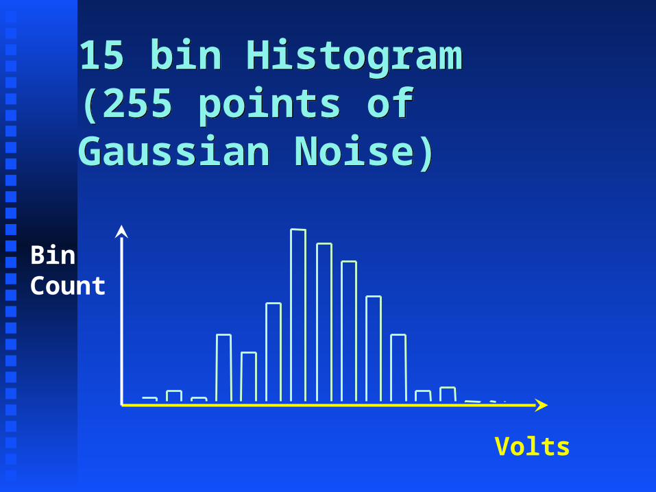
15 bin Histogram(255 points of Gaussian Noise)15 bin Histogram(255 points of Gaussian Noise)

Volts

BinCount

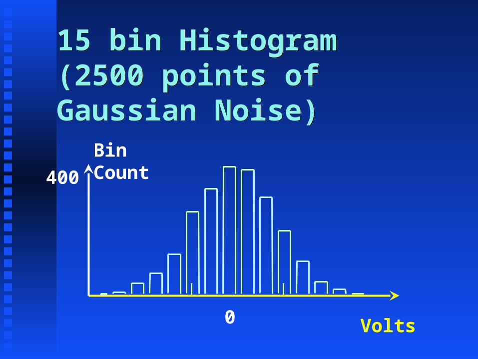
15 bin Histogram(2500 points of Gaussian Noise)15 bin Histogram(2500 points of Gaussian Noise)

Volts

BinCount

0

400

Previous waveformsPrevious waveforms

Are all 0 mean, 1 watt, White Noise Are all 0 mean, 1 watt, White Noise

0

0

Autocorrelation & Power Spectrum of White NoiseAutocorrelation & Power Spectrum of White Noise

Rx(tau)

tau seconds0

A

Gx(f)

Hertz0

A watts/Hz

The previous WhiteNoise waveforms all

have same Autocorrelation& Power Spectrum.

Autocorrelation (& Power Spectrum)

versus Probability Density Function

Autocorrelation (& Power Spectrum)

versus Probability Density Function Autocorrelation: Time axis predictabilityAutocorrelation: Time axis predictability

PDF: Voltage liklihoodPDF: Voltage liklihood Autocorrelation provides Autocorrelation provides NONO information about the information about the

PDF (& vice-versa)...PDF (& vice-versa)... ......EXCEPTEXCEPT the power will be the same...the power will be the same...

PDF second moment E[XPDF second moment E[X22] = R] = Rxx(0) = area(0) = area

under Power Spectrum = A{x(t) under Power Spectrum = A{x(t)22}} ......ANDAND the D.C. value will be related. the D.C. value will be related.

PDF first moment squared E[X] PDF first moment squared E[X]22 = constant = constant term in autocorrelation = E[X] term in autocorrelation = E[X]22δδ(f) = A{x(t)}(f) = A{x(t)}22

Satellite vs Sun, Daytime, Northern HemisphereSatellite vs Sun, Daytime, Northern Hemisphere

x

WinterSun is belowsatelliteorbital plane.

x

Fall Sun → sameplane assatellite.

x

Spring Sun→ sameplane asSatellite.

x

SummerSun is abovesatelliteorbital plane.

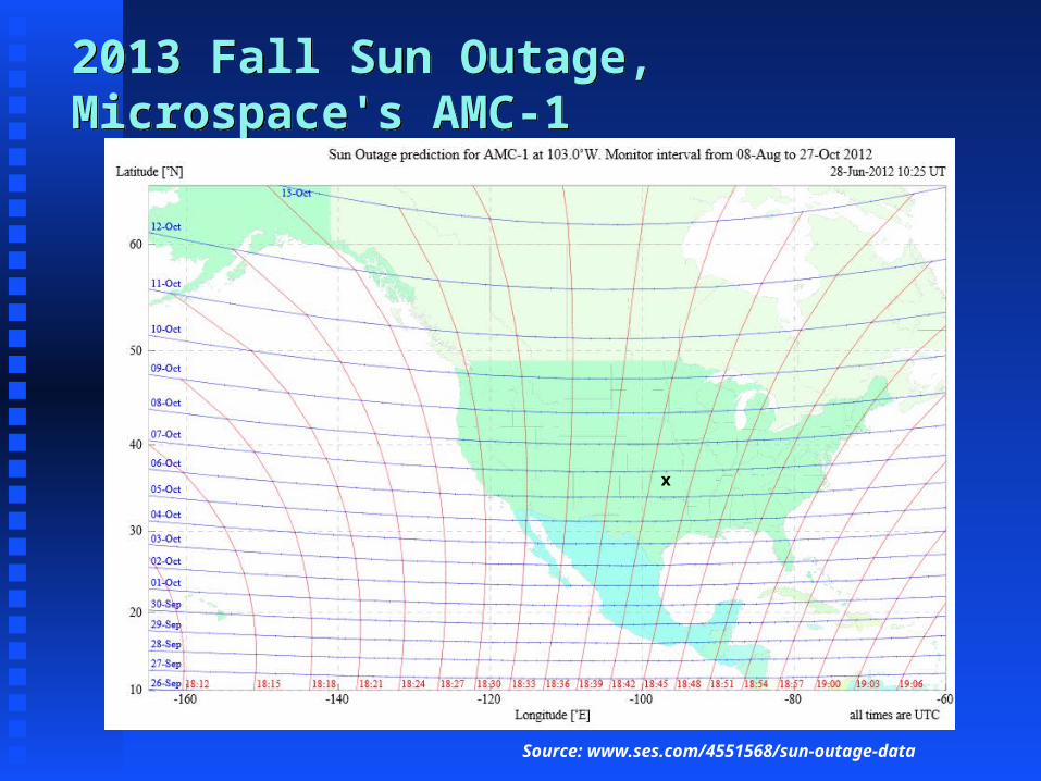
2013 Fall Sun Outage, Microspace's AMC-12013 Fall Sun Outage, Microspace's AMC-1

Source: www.ses.com/4551568/sun-outage-data

x

Band Limited Continuous TimeWhite Noise Waveforms

(255 point Gaussian Noise)

Band Limited Continuous TimeWhite Noise Waveforms

(255 point Gaussian Noise)

Time

Volts

0

If AC power = 4 watts & BW = 1,000 GHz...

Probability Density Function of Band Limited Gausssian White Noise

Probability Density Function of Band Limited Gausssian White Noise

fx(x)

Volts0

.399/σx = .399/2 = 0.1995Time

Volts

0

Autocorrelation & Power Spectrum of Bandlimited Gaussian White Noise

Autocorrelation & Power Spectrum of Bandlimited Gaussian White Noise

Rx(tau)

tau seconds0

Gx(f)

Hertz0

2(10-12) watts/Hz

-1000 GHz

4

500(10-15)

How does PDF, Rx(τ), & GX(f)change if +3 volts added?

(255 point Gaussian Noise)

How does PDF, Rx(τ), & GX(f)change if +3 volts added?

(255 point Gaussian Noise)

Time

Volts

3

AC power = 4 watts

0

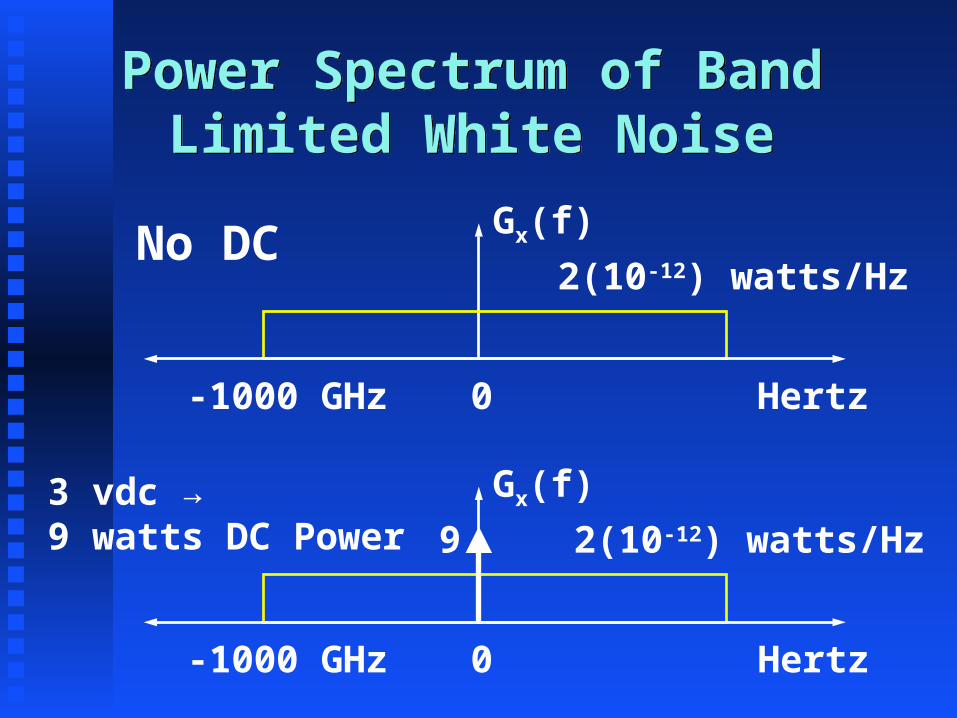
Power Spectrum of Band Limited White Noise

Power Spectrum of Band Limited White Noise

Gx(f)

Hertz0-1000 GHz

9

Gx(f)

Hertz0

2(10-12) watts/Hz

-1000 GHz

2(10-12) watts/Hz

No DC

3 vdc → 9 watts DC Power

Autocorrelation of Band Limited White Noise

Autocorrelation of Band Limited White Noise

Rx(tau)

tau seconds0

13

9

Rx(tau)

tau seconds0

4

500(10-15)

500(10-15)

No DC

3 vdc → 9 watts DC Power

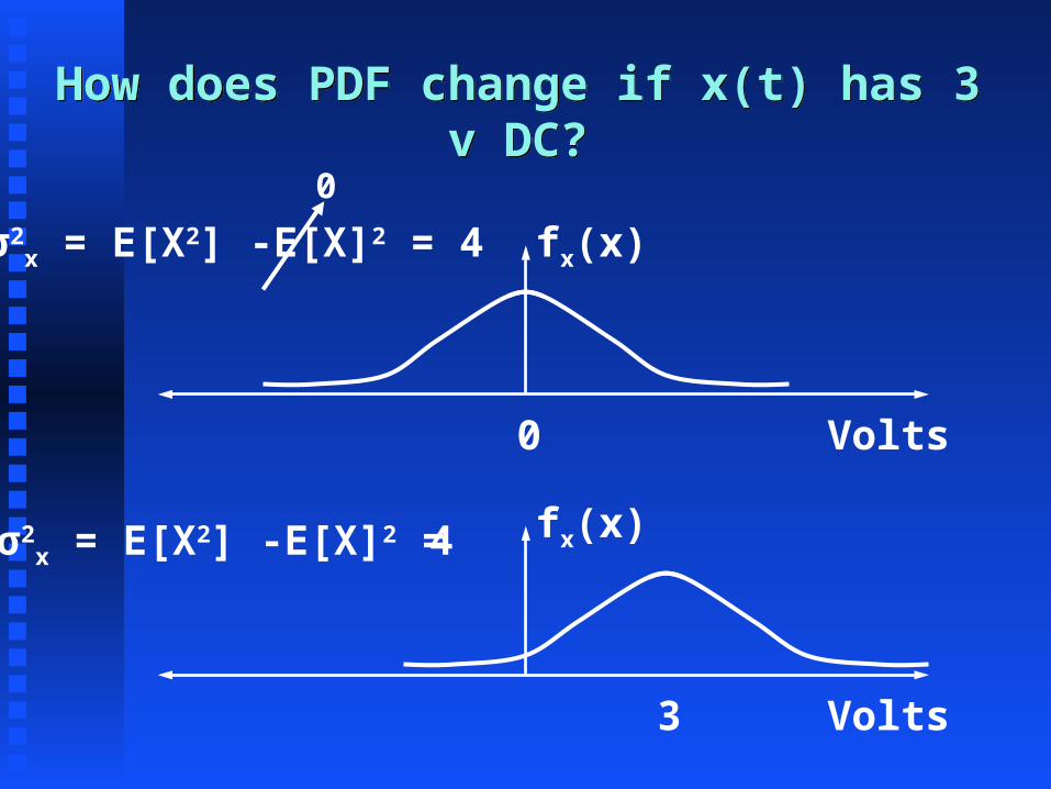
How does PDF change if x(t) has 3 v DC?How does PDF change if x(t) has 3 v DC?

fx(x)

Volts0

σ2x = E[X2] -E[X]2 = 4

0

fx(x)

Volts3

σ2x = E[X2] -E[X]2 = 4

Band Limited Continuous TimeWhite Noise Waveforms

(255 point Gaussian Noise)

Band Limited Continuous TimeWhite Noise Waveforms

(255 point Gaussian Noise)

Time

Volts

3

AC power = 4 wattsDC power = 9 wattsTotal Power = 13 watts

0

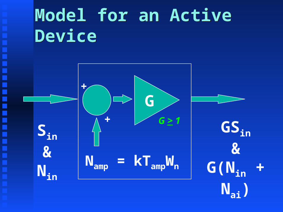
Model for an Active DeviceModel for an Active Device

Sin

&Nin

GSin

&G(Nin + Nai)

G

Namp = kTampWn

+

+

G > 1

Noise FigureNoise Figure

F = SNRF = SNRinin/SNR/SNRoutout

WARNING! Use with caution.WARNING! Use with caution.If input noise changes, F will change. If input noise changes, F will change.

F = 1 + TF = 1 + Tampamp/T/Tinin

TTin in = 290= 290oo K (default) K (default)

Model for a Passive DeviceModel for a Passive Device

Sin

&Nin

GSin

&G(Nin + Nai)

G

Namp = kTpassiveWn

+

+

G < 1

Tpassive = (L-1)Tphysical

Temperatures...Temperatures...

Active Device (TActive Device (Tampamp) ) From Spec Sheet (may have F)From Spec Sheet (may have F)

Passive Device (TPassive Device (Tcable cable or Tor T passive passive))

(L-1)*T(L-1)*Tphysicalphysical

System Noise (Actual)System Noise (Actual)Noise Striking Antenna = NoWThermal

= kTsurroundings1000*109 = k*290*1000*109

= 4.00 n watts

Much of this noise doesn't exit system.Blocked by system filters. kTantWN = ???

SystemCable + Amp

Noise exiting Antenna that will exit the System =kTant6*106 = 12.42*10-15 watts

Noise Antenna "Sees" = Noise exiting antenna = NoWAntenna

≈ kTant1000*109 = 2.07 n watts

(Tantenna = 150 Kelvin)

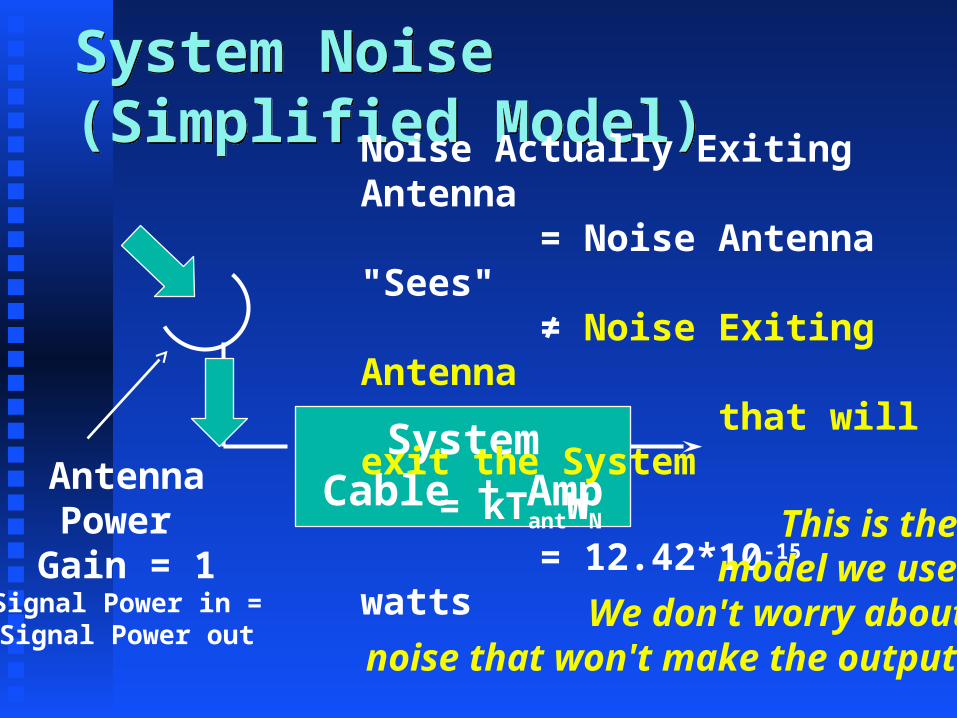
System Noise (Simplified Model)System Noise (Simplified Model)

SystemCable + Amp

Noise Actually Exiting Antenna = Noise Antenna "Sees" ≠ Noise Exiting Antenna that will exit the System = kTantWN = 12.42*10-15 watts

AntennaPower

Gain = 1Signal Power in =Signal Power out

This is the model we use.

We don't worry aboutnoise that won't make the output.

SNR Considering all the noiseSNR Considering all the noiseNoise Seen by Antenna = NoWAntenna

= kTant1000*109 = 2.07 n wattsSignal Power Picked Up by Antenna = 10-11 watts

SystemCable + Amp

SNR at "input" of antenna = 10-11/(4*10-9) = 0.0025SNR at output of antenna = 10-11/(2.07*10-9) = 0.004831SNR at System Output = 43.63

SNR Considering Noise Hitting Antenna That Can Reach the Output

SNR Considering Noise Hitting Antenna That Can Reach the Output

Noise seen by Antenna TCRO = NoWN

= kTant6*106 = 12.42 femto wattsSignal Power Picked Up by Antenna = 10-11 watts

SystemCable + Amp

SNR at output of antenna = 805.2

SNR at System Output = 43.63

This is the noise we're

worried about.

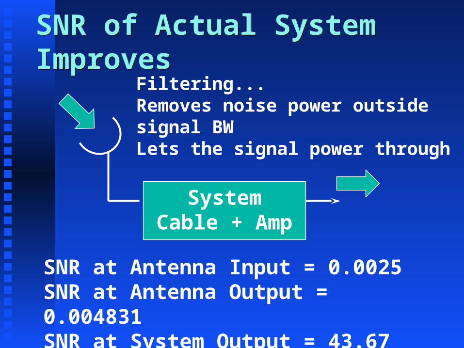
SNR of Actual System ImprovesSNR of Actual System ImprovesFiltering...Removes noise power outside signal BWLets the signal power through

SystemCable + Amp

SNR at Antenna Input = 0.0025SNR at Antenna Output = 0.004831SNR at System Output = 43.67

SNR of Model WorsensSNR of Model WorsensOnly considers input noise that is in the signal BW & can reach the output.Cable & electronics dump in more

noise.

SystemCable + Amp

SNR at antenna output = 805.2 SNR at System Output = 43.67