Embed Size (px)
Citation preview
Lecture 22: Voltage Stability, PV and QV
Curves, Geomagnetic Disturbances
ECEN 615Methods of Electric Power Systems Analysis
Prof. Tom Overbye
Dept. of Electrical and Computer Engineering
Texas A&M University
Announcements
• Homework 5 is due today
• Homework 6 is due on Tuesday Nov 27
• Read Chapters 3 and 8 (Economic Dispatch and
Optimal Power Flow)
2
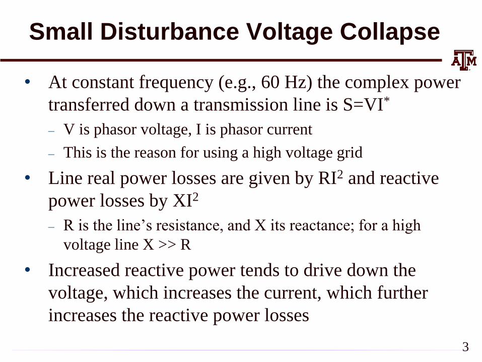
Small Disturbance Voltage Collapse
• At constant frequency (e.g., 60 Hz) the complex power
transferred down a transmission line is S=VI*
– V is phasor voltage, I is phasor current
– This is the reason for using a high voltage grid
• Line real power losses are given by RI2 and reactive
power losses by XI2
– R is the line’s resistance, and X its reactance; for a high
voltage line X >> R
• Increased reactive power tends to drive down the
voltage, which increases the current, which further
increases the reactive power losses
3
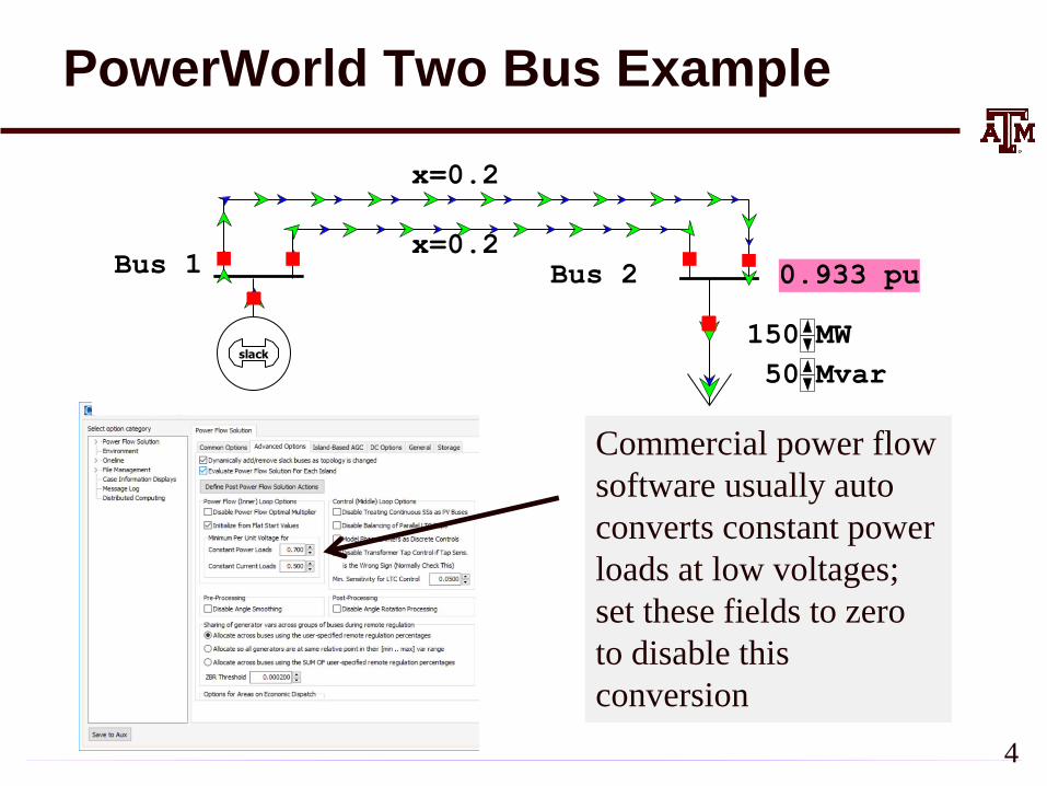
PowerWorld Two Bus Example
slack
Bus 1 Bus 2
x=0.2
x=0.20.933 pu
MW 150
Mvar 50
Commercial power flow
software usually auto
converts constant power
loads at low voltages;
set these fields to zero
to disable this
conversion
4
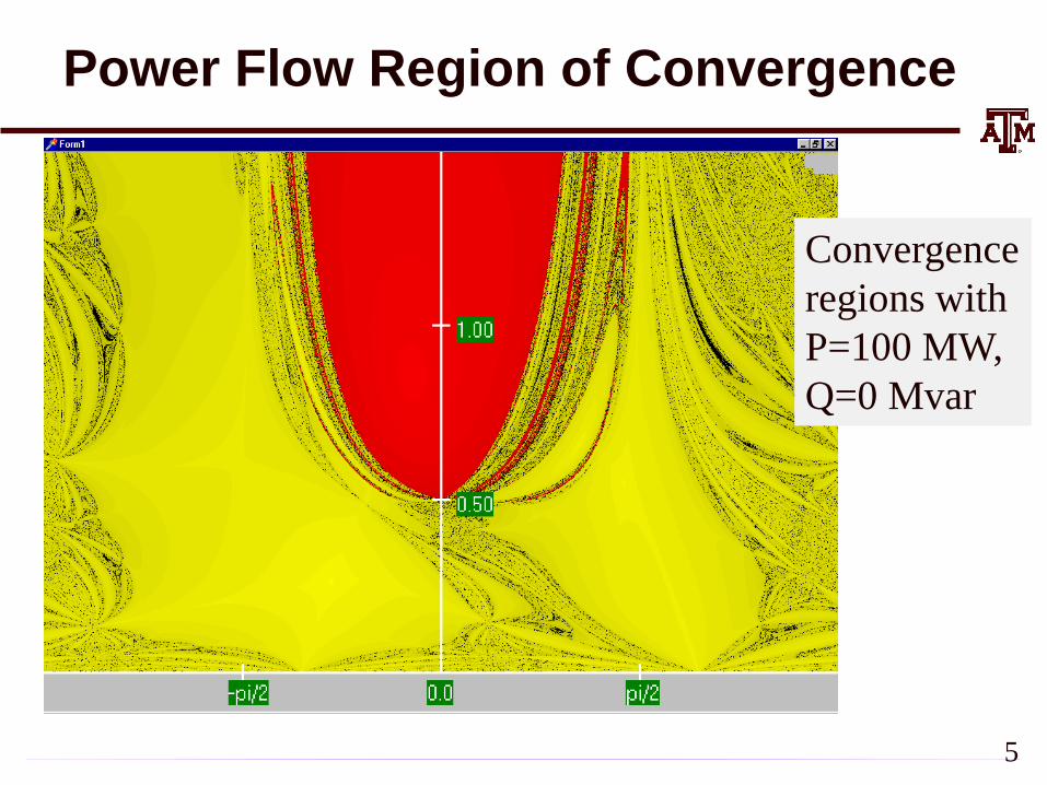
Power Flow Region of Convergence
Convergence
regions with
P=100 MW,
Q=0 Mvar
5
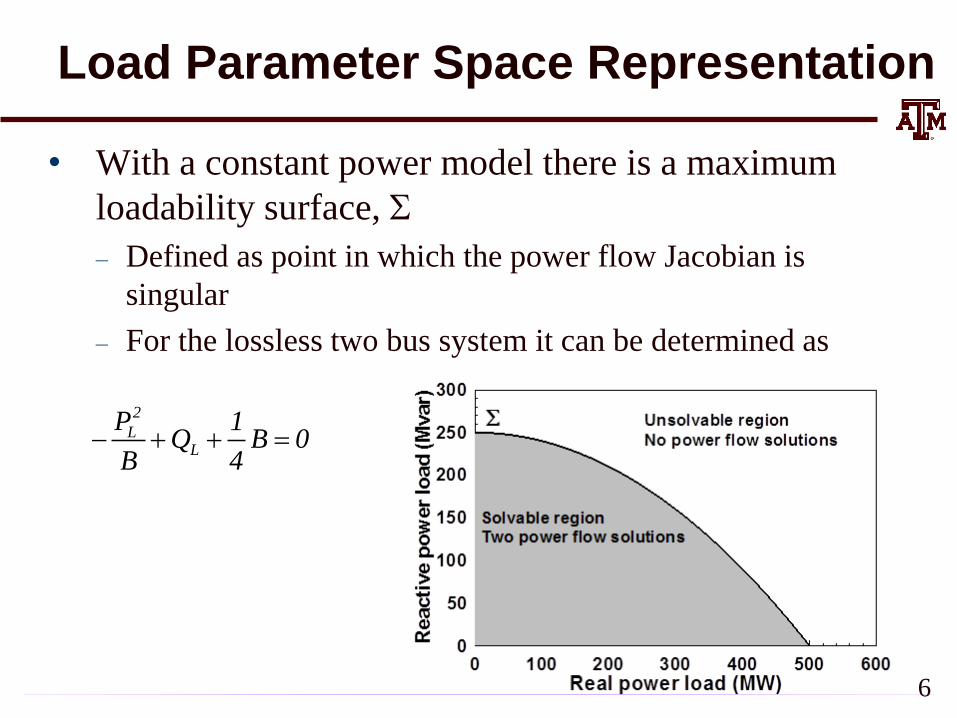
Load Parameter Space Representation
• With a constant power model there is a maximum
loadability surface, S
– Defined as point in which the power flow Jacobian is
singular
– For the lossless two bus system it can be determined as
2
LL
P 1Q B 0
B 4
6
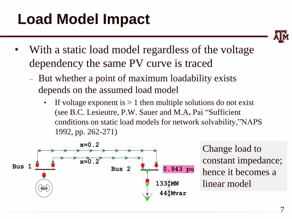
Load Model Impact
• With a static load model regardless of the voltage
dependency the same PV curve is traced
– But whether a point of maximum loadability exists
depends on the assumed load model
• If voltage exponent is > 1 then multiple solutions do not exist
(see B.C. Lesieutre, P.W. Sauer and M.A. Pai “Sufficient
conditions on static load models for network solvability,”NAPS
1992, pp. 262-271)
7
slack
Bus 1 Bus 2
x=0.2
x=0.2
0.943 pu
MW 133
Mvar 44
Change load to
constant impedance;
hence it becomes a
linear model
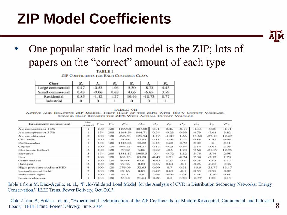
ZIP Model Coefficients
• One popular static load model is the ZIP; lots of
papers on the “correct” amount of each type
Table 7 from A, Bokhari, et. al., “Experimental Determination of the ZIP Coefficients for Modern Residential, Commercial, and Industrial
Loads,” IEEE Trans. Power Delivery, June. 2014
Table 1 from M. Diaz-Aguilo, et. al., “Field-Validated Load Model for the Analysis of CVR in Distribution Secondary Networks: Energy
Conservation,” IEEE Trans. Power Delivery, Oct. 2013
8
Application: Conservation Voltage Reduction (CVR)
• If the “steady-state” load has a true dependence on
voltage, then a change (usually a reduction) in the
voltage should result in a total decrease in energy
consumption
• If an “optimal” voltage could be determined, then this
could result in a net energy savings
• Some challenges are 1) the voltage profile across a
feeder is not constant, 2) the load composition is
constantly changing, 3) a decrease in power
consumption might result in a decrease in useable
output from the load, and 4) loads are dynamic and an
initial increase might be balanced by a later increase 9
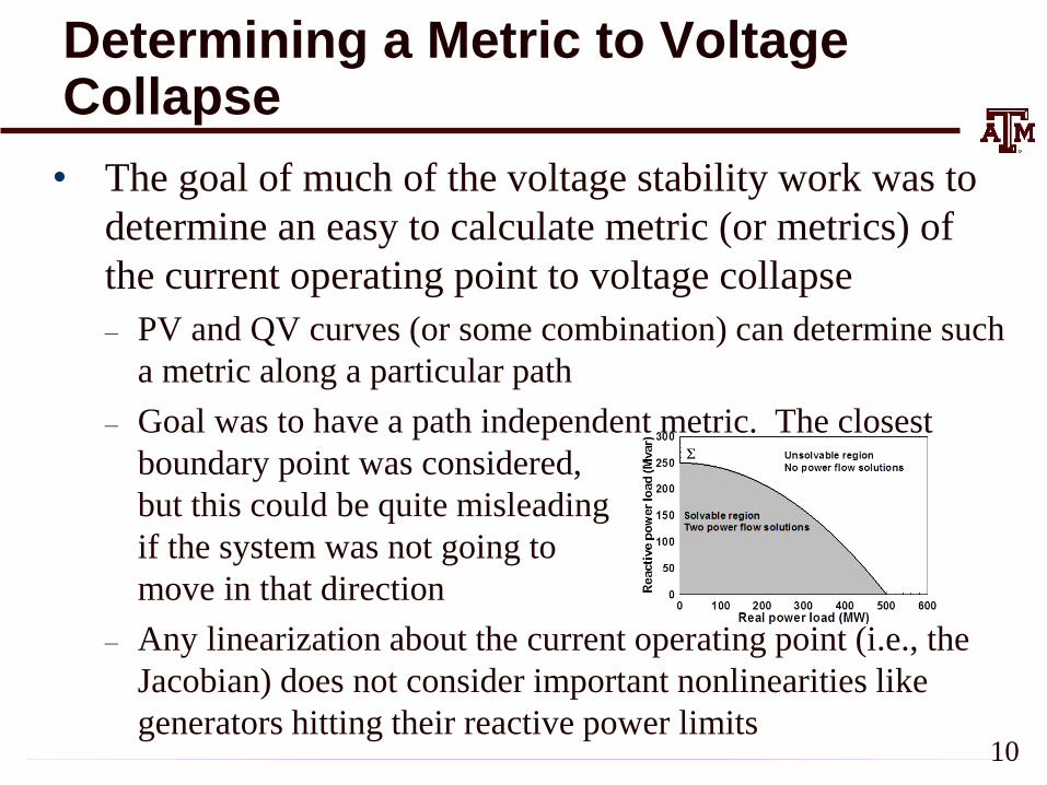
Determining a Metric to Voltage Collapse
• The goal of much of the voltage stability work was to
determine an easy to calculate metric (or metrics) of
the current operating point to voltage collapse
– PV and QV curves (or some combination) can determine such
a metric along a particular path
– Goal was to have a path independent metric. The closest
boundary point was considered,
but this could be quite misleading
if the system was not going to
move in that direction
– Any linearization about the current operating point (i.e., the
Jacobian) does not consider important nonlinearities like
generators hitting their reactive power limits 10
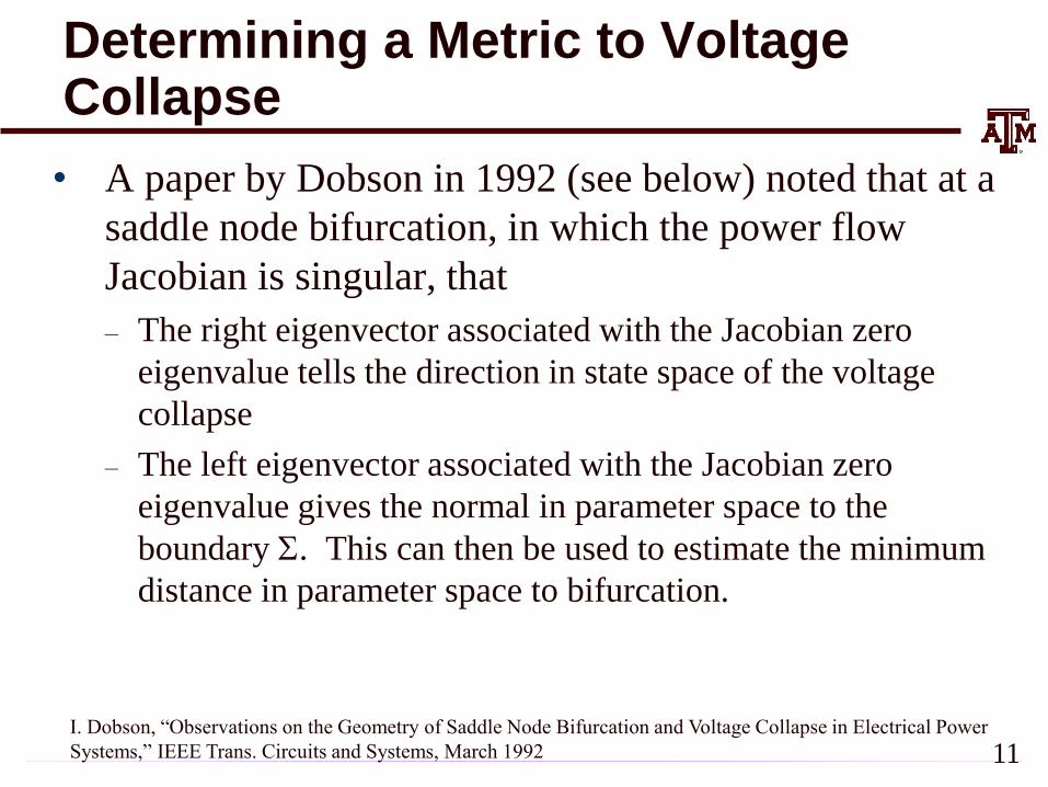
Determining a Metric to Voltage Collapse
• A paper by Dobson in 1992 (see below) noted that at a
saddle node bifurcation, in which the power flow
Jacobian is singular, that
– The right eigenvector associated with the Jacobian zero
eigenvalue tells the direction in state space of the voltage
collapse
– The left eigenvector associated with the Jacobian zero
eigenvalue gives the normal in parameter space to the
boundary S. This can then be used to estimate the minimum
distance in parameter space to bifurcation.
I. Dobson, “Observations on the Geometry of Saddle Node Bifurcation and Voltage Collapse in Electrical Power
Systems,” IEEE Trans. Circuits and Systems, March 1992 11
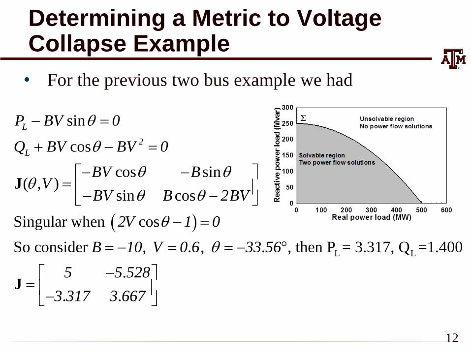
Determining a Metric to Voltage Collapse Example
• For the previous two bus example we had
L L
sin
cos
cos sin( , )
sin cos
Singular when cos
So consider , . , . , then P = 3.317, Q =1.400
.
. .
L
2
L
P BV 0
Q BV BV 0
BV BV
BV B 2BV
2V 1 0
B 10 V 0 6 33 56
5 5 528
3 317 3 667
J
J
12
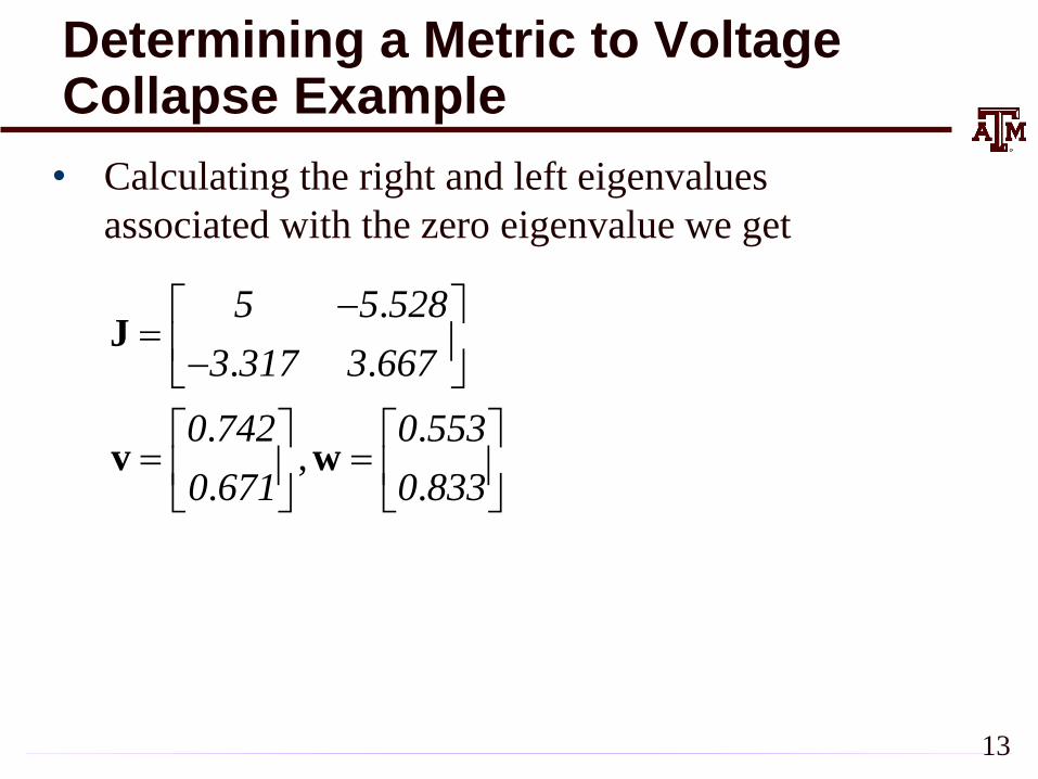
Determining a Metric to Voltage Collapse Example
• Calculating the right and left eigenvalues
associated with the zero eigenvalue we get
.
. .
. .,
. .
5 5 528
3 317 3 667
0 742 0 553
0 671 0 833
J
v w
13
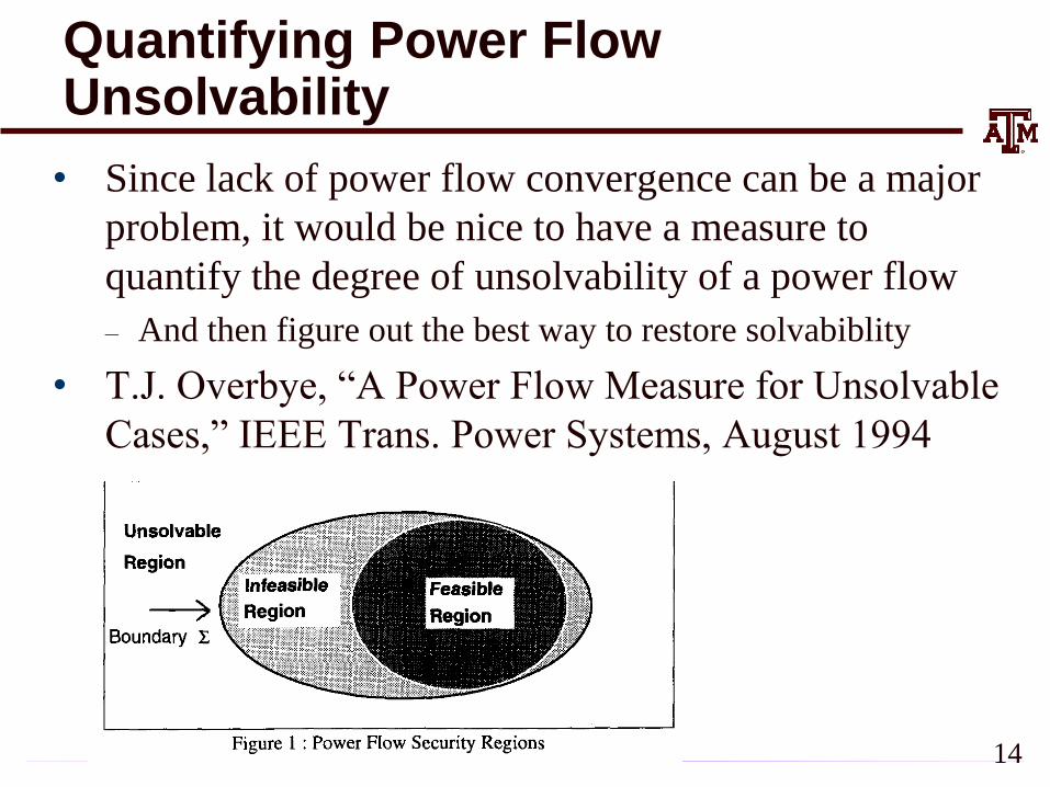
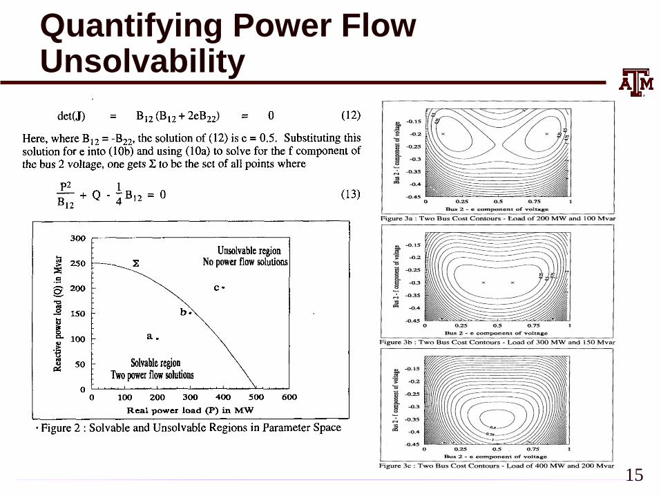
Quantifying Power Flow Unsolvability
• Since lack of power flow convergence can be a major
problem, it would be nice to have a measure to
quantify the degree of unsolvability of a power flow
– And then figure out the best way to restore solvabiblity
• T.J. Overbye, “A Power Flow Measure for Unsolvable
Cases,” IEEE Trans. Power Systems, August 1994
14
Quantifying Power Flow Unsolvability
15
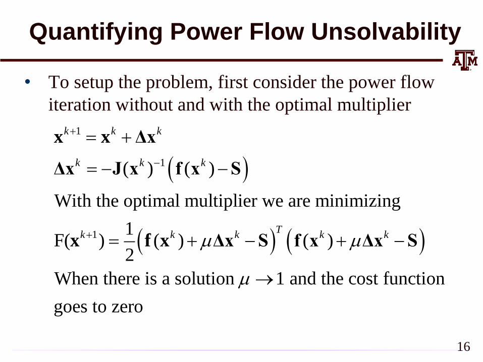
Quantifying Power Flow Unsolvability
• To setup the problem, first consider the power flow
iteration without and with the optimal multiplier
1
1
1
( ) ( )
With the optimal multiplier we are minimizing
1F( ) ( ) ( )
2
When there is a solution 1 and the cost function
goes to zero
k k k
k k k
Tk k k k k
x x Δx
Δx J x f x S
x f x Δx S f x Δx S
16
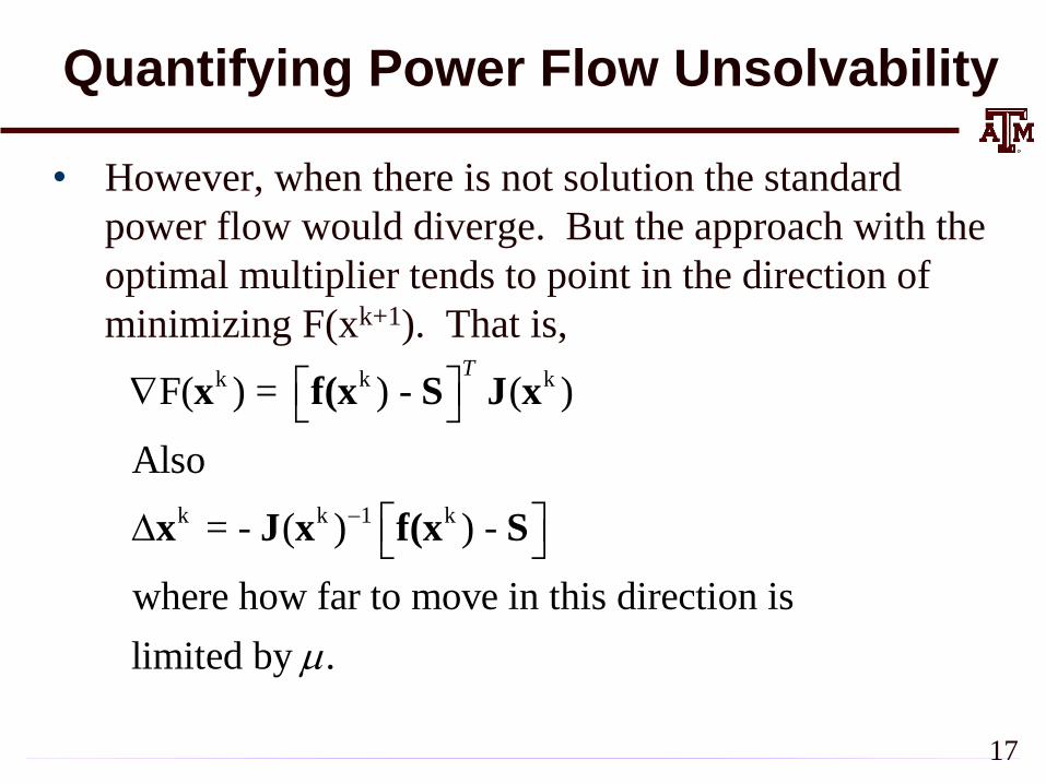
Quantifying Power Flow Unsolvability
• However, when there is not solution the standard
power flow would diverge. But the approach with the
optimal multiplier tends to point in the direction of
minimizing F(xk+1). That is,
17
k k k
k k 1 k
F( ) = ) - ( )
Also
= - ( ) ) -
where how far to move in this direction is
limited by .
T
x f(x S J x
x J x f(x S
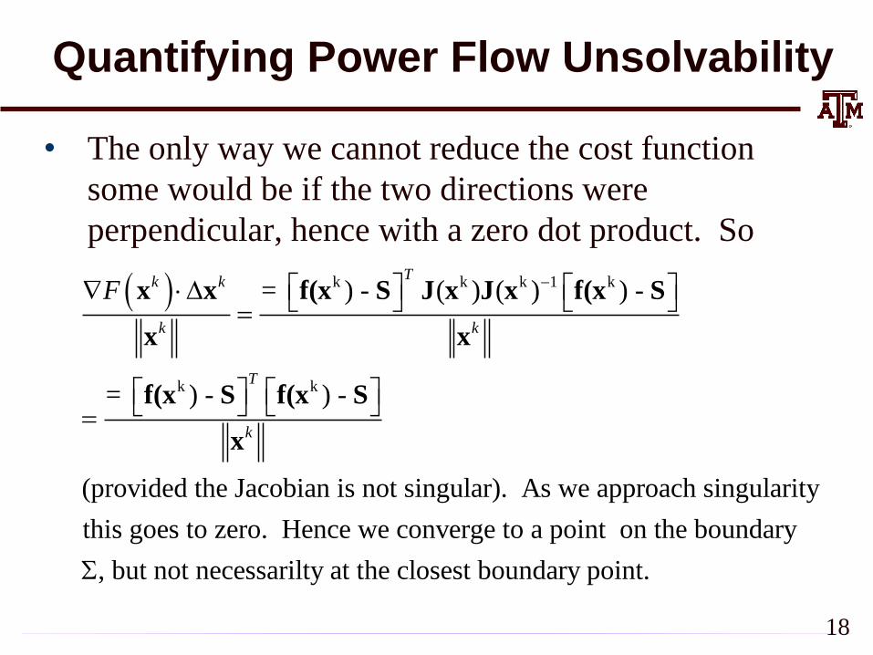
Quantifying Power Flow Unsolvability
• The only way we cannot reduce the cost function
some would be if the two directions were
perpendicular, hence with a zero dot product. So
18
k k k 1 k
k k
= ) - ( ) ( ) ) -
= ) - ) -
(provided the Jacobian is not singular). As we approach singularity
this goes to zero. Hence we converge to a poi
Tk k
k k
T
k
F
x x f(x S J x J x f(x S
x x
f(x S f(x S
x
nt on the boundary
, but not necessarilty at the closest boundary point. S
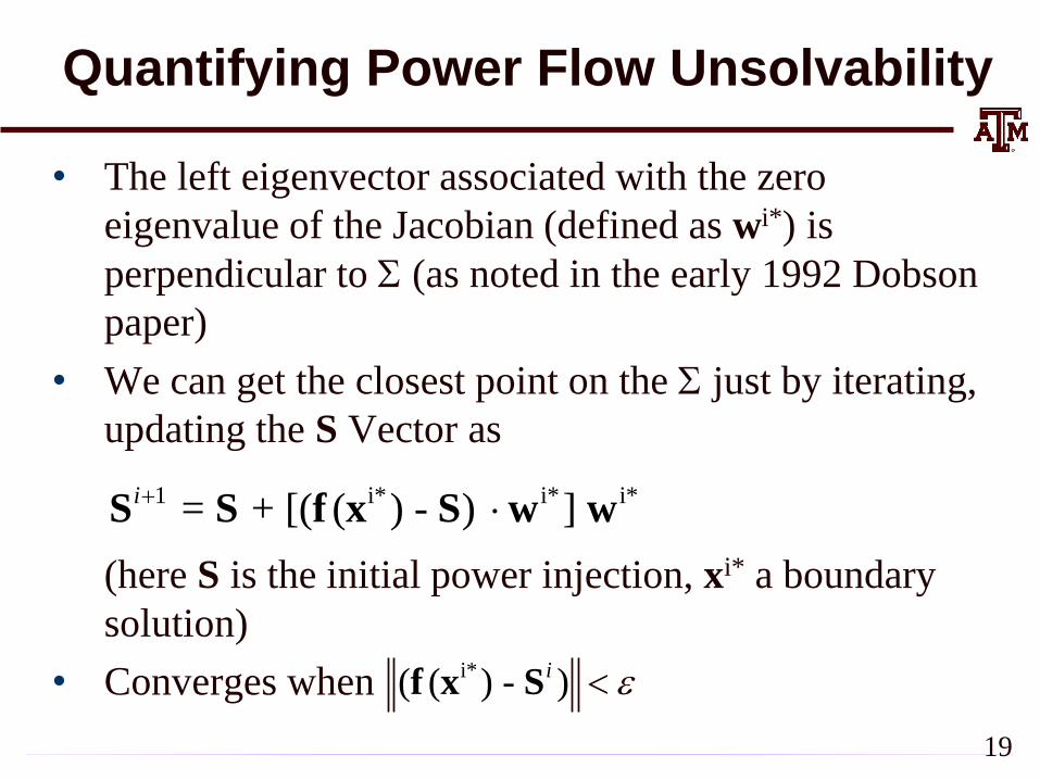
Quantifying Power Flow Unsolvability
• The left eigenvector associated with the zero
eigenvalue of the Jacobian (defined as wi*) is
perpendicular to S (as noted in the early 1992 Dobson
paper)
• We can get the closest point on the S just by iterating,
updating the S Vector as
(here S is the initial power injection, xi* a boundary
solution)
• Converges when
1 i* i* i* = + [( ( ) - ) ] i S S f x S w w
19
i*( ( ) - )i f x S
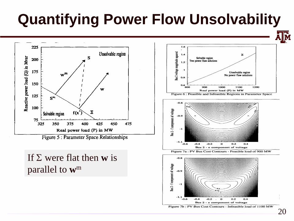
Quantifying Power Flow Unsolvability
20
If S were flat then w is
parallel to wm
Challenges
• The key issues is actual power systems are quite
complex, with many nonlinearities. For example,
generators hitting reactive power limits, switched
shunts, LTCs, phase shifters, etc.
• Practically people would like to know how far some
system parameters can be changed before running into
some sort of limit violation, or maximum loadability.
– The system is changing in a particular direction, such as a
power transfer; his often includes contingency analysis
• Line limits and voltage magnitudes are considered
– Lower voltage lines tend to be thermally constrained
• Solution is to just to trace out the PV or QV curves 21
PV and QV Analysis in PowerWorld
• Requires setting up what is known in PowerWorld as
an injection group
– An injection group specifies a set of objects, such as
generators and loads, that can inject or absorb power
– Injection groups can be defined by selecting Case
Information, Aggregation, Injection Groups
• The PV and/or QV analysis then varies the injections
in the injection group, tracing out the PV curve
• This allows optional consideration of contingencies
• The PV tool can be displayed by selecting Add-Ons,
PV
22
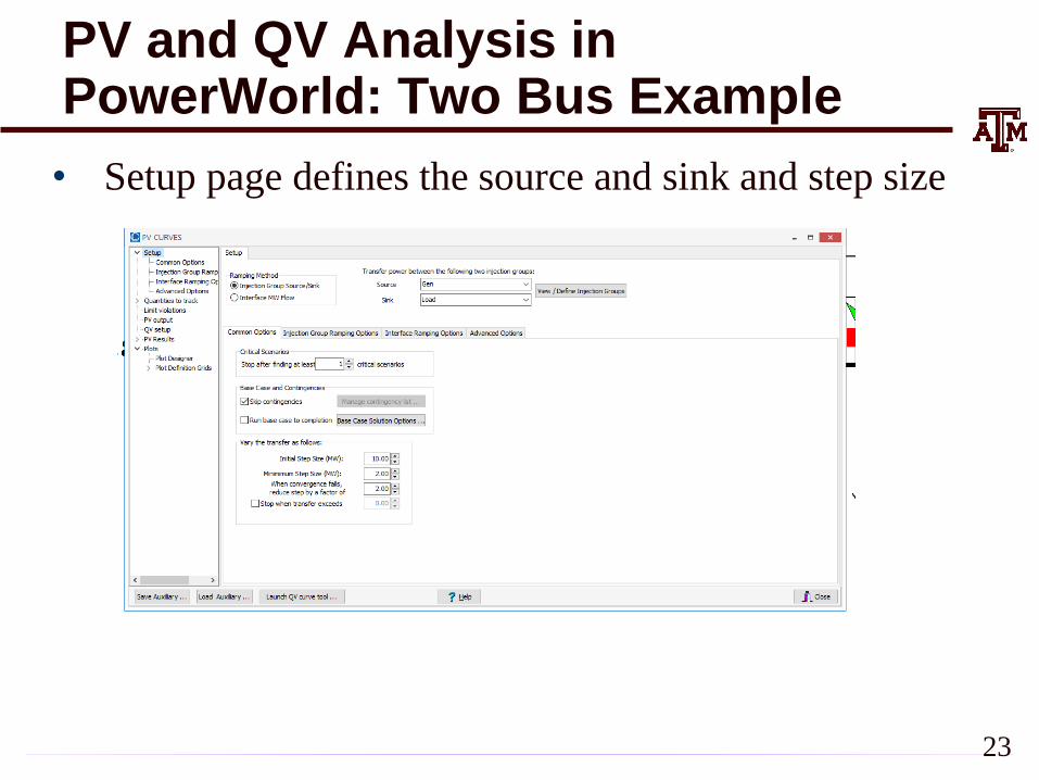
PV and QV Analysis in PowerWorld: Two Bus Example
• Setup page defines the source and sink and step size
23
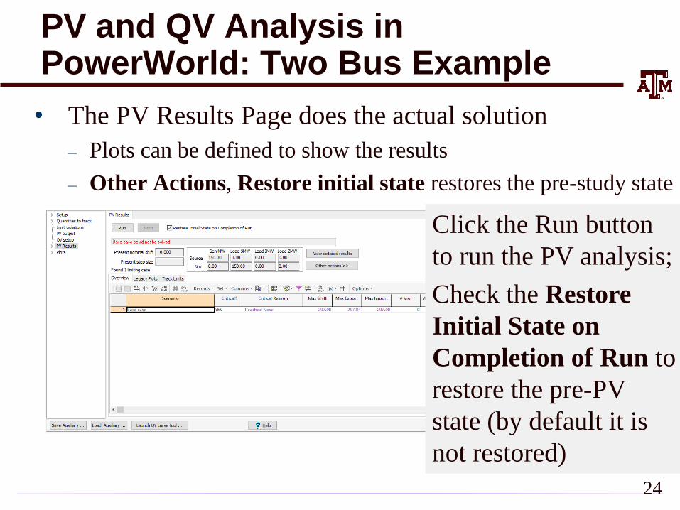
PV and QV Analysis in PowerWorld: Two Bus Example
• The PV Results Page does the actual solution
– Plots can be defined to show the results
– Other Actions, Restore initial state restores the pre-study state
24
Click the Run button
to run the PV analysis;
Check the Restore
Initial State on
Completion of Run to
restore the pre-PV
state (by default it is
not restored)
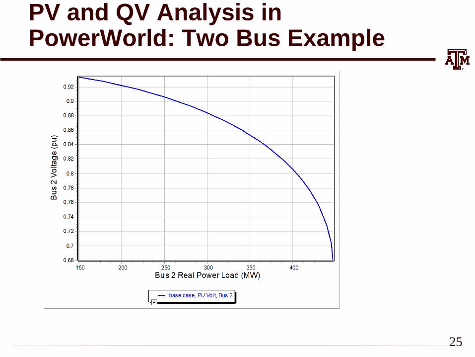
PV and QV Analysis in PowerWorld: Two Bus Example
25
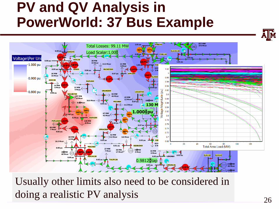
PV and QV Analysis in PowerWorld: 37 Bus Example
slack
SLACK138
PINE345
PINE138
PINE69
PALM69
LOCUST69
PEAR69
PEAR138
CEDAR138
CEDAR69
WILLOW69
OLIVE69
BIRCH69
PECAN69
ORANGE69
MAPLE69
OAK69
OAK138
OAK345
BUCKEYE69
APPLE69
WALNUT69
MAPLE69
POPLAR69
PEACH69
ASH138
PEACH138
SPRUCE69
CHERRY69
REDBUD69
TULIP138
LEMON69
LEMON138
ELM138 ELM345
20%A
MVA
57%A
MVA
73%A
MVA
38%A
MVA
58%A
MVA
46%A
MVA
46%A
MVA
A
MVA
67%A
MVA
15%A
MVA
27%A
MVA
80%A
MVA
34%A
MVA
69%A
MVA
21%A
MVA
79%A
MVA
12%A
MVA
49%A
MVA
15%A
MVA
18%A
MVA
A
MVA
14%A
MVA
56%A
MVA
79%A
MVA
73%A
MVA
71%A
MVA
85%A
MVA
1.01 pu
0.98 pu
1.01 pu
1.03 pu
0.96 pu
0.96 pu
0.99 pu
0.97 pu
0.97 pu
0.95 pu
0.97 pu
0.96 pu
0.97 pu
0.96 pu
0.99 pu
0.90 pu
0.90 pu
0.95 pu
0.787 pu
0.78 pu
0.82 pu
0.90 pu
0.90 pu
0.93 pu
0.91 pu
0.93 pu 0.92 pu
0.94 pu
0.93 pu0.93 pu
1.02 pu
69%A
MVA
PLUM138
16%A
MVA
0.99 pu
A
MVA
0.95 pu
70%A
MVA
877 MW 373 Mvar
24 MW
0 Mvar
42 MW
12 MvarMW 180
130 Mvar
60 MW
16 Mvar
14 MW 6 Mvar
MW 150
60 Mvar
64 MW
14 Mvar
44 MW 12 Mvar
42 MW
4 Mvar
49 MW
0 Mvar
67 MW
42 Mvar
42 MW
12 Mvar
MW 10
5 Mvar
26 MW
17 Mvar
69 MW
14 Mvar
MW 20
40 Mvar
26 MW
10 Mvar
38 MW
15 Mvar 14.3 Mvar 21 MW
6 Mvar
66 MW
46 Mvar 297 MW
19 Mvar
Mvar 0.0
126 MW
8 Mvar
89 MW 7 Mvar
27 MW
7 Mvar 16 MW
0 Mvar
7.8 Mvar
6.0 Mvar
11.5 Mvar
26.0 Mvar
6.8 Mvar
16.3 Mvar
MW 106
60 Mvar
22 MW
9 Mvar
MW 150
60 Mvar
19 MW
3 Mvar
MW 16
26 Mvar
35 MW
12 Mvar
Total Losses: 99.11 MW
80%A
MVApu 1.000
tap0.9812
Load Scalar:1.00
90%A
MVA
86%A
MVA
90%A
MVA
89%A
MVA
88%A
MVA
94%A
MVA
94%A
MVA
96%A
MVA
97%A
MVA
104%A
MVA
115%A
MVA217%A
MVA
130%A
MVA
136%A
MVA
103%A
MVA
103%A
MVA
325%A
MVA
132%A
MVA
113%A
MVA
114%A
MVA
122%A
MVA
111%A
MVA
112%A
MVA
102%A
MVA
26
Usually other limits also need to be considered in
doing a realistic PV analysis
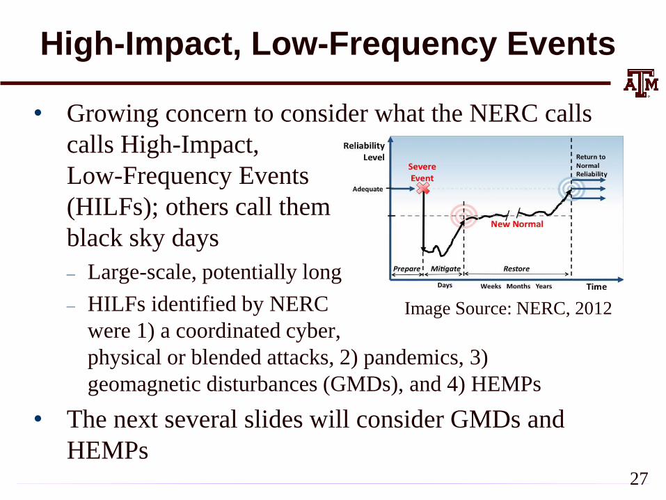
High-Impact, Low-Frequency Events
• Growing concern to consider what the NERC calls
calls High-Impact,
Low-Frequency Events
(HILFs); others call them
black sky days
– Large-scale, potentially long duration blackouts
– HILFs identified by NERC
were 1) a coordinated cyber,
physical or blended attacks, 2) pandemics, 3)
geomagnetic disturbances (GMDs), and 4) HEMPs
• The next several slides will consider GMDs and
HEMPs
Image Source: NERC, 2012
27
Geomagnetic Disturbances (GMDs)
• GMDs are caused by solar corona mass ejections
(CMEs) impacting the earth’s magnetic field
• A GMD caused a blackout in 1989 of Quebec
• They have the potential to severely disrupt the
electric grid by causing quasi-dc geomagnetically
induced currents (GICs) in the high voltage grid
• Until recently power engineers had few tools to
help them assess the impact of GMDs
• GMD assessment tools are now moving into the
realm of power system planning and operations
engineers; required by NERC Standards (TPL
007-1, 007-2) 28
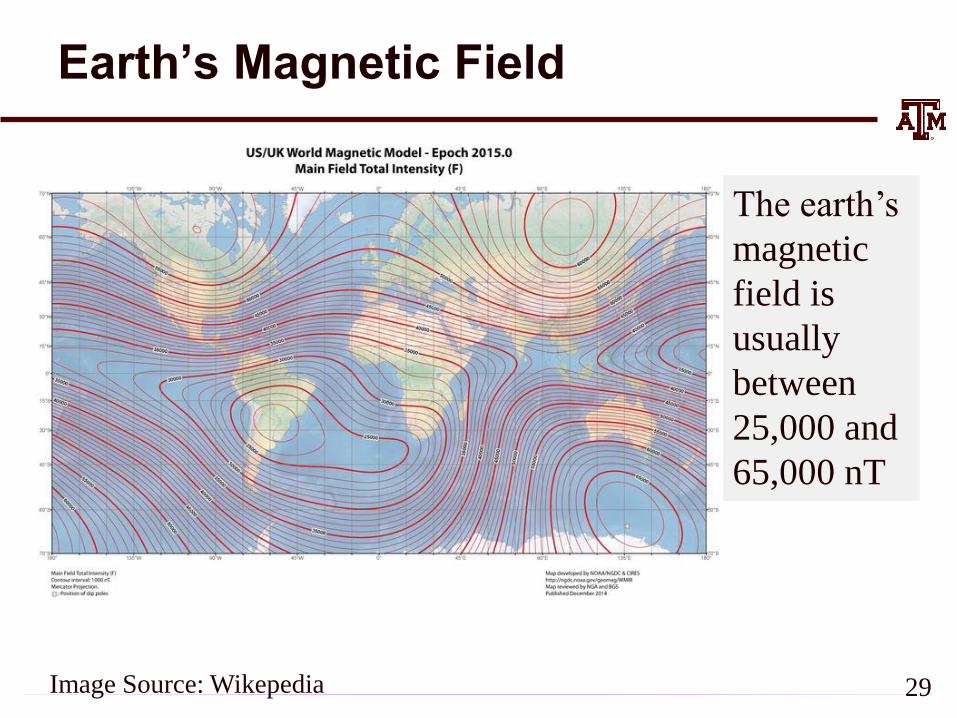
Earth’s Magnetic Field
29Image Source: Wikepedia
The earth’s
magnetic
field is
usually
between
25,000 and
65,000 nT
Earth’s Magnetic Field Variations
• The earth’s magnetic field is constantly changing,
though usually the variations are not significant
– Larger changes tend to occur closer to the earth’s magnetic
poles
• The magnitude of the variation at any particular location
is quantified with a value known as the K-index
– Ranges from 1 to 9, with the value dependent on nT variation
in horizontal direction over a three hour period
– This is station specific; higher variations are required to get a
k=9 closer to the poles
• The Kp-index is a weighted average of the individual
station K-indices; G scale approximately is Kp - 430
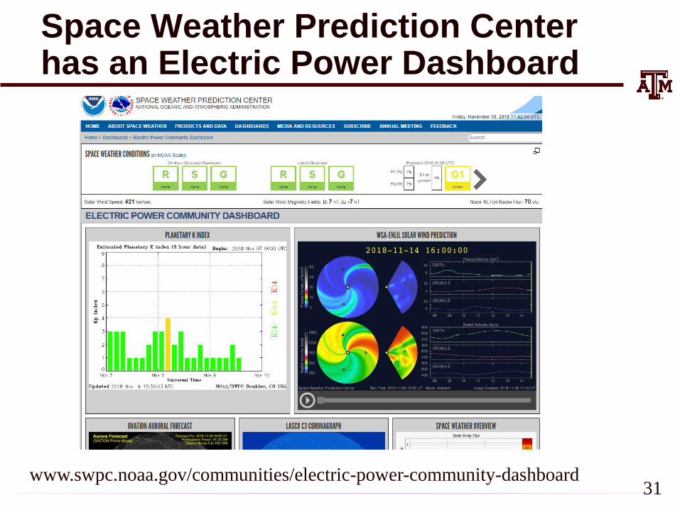
Space Weather Prediction Center has an Electric Power Dashboard
www.swpc.noaa.gov/communities/electric-power-community-dashboard31
GMD and the Grid
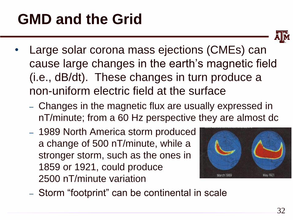
• Large solar corona mass ejections (CMEs) can
cause large changes in the earth’s magnetic field
(i.e., dB/dt). These changes in turn produce a
non-uniform electric field at the surface
– Changes in the magnetic flux are usually expressed in
nT/minute; from a 60 Hz perspective they are almost dc
– 1989 North America storm produced
a change of 500 nT/minute, while a
stronger storm, such as the ones in
1859 or 1921, could produce
2500 nT/minute variation
– Storm “footprint” can be continental in scale
32
Solar Cycles
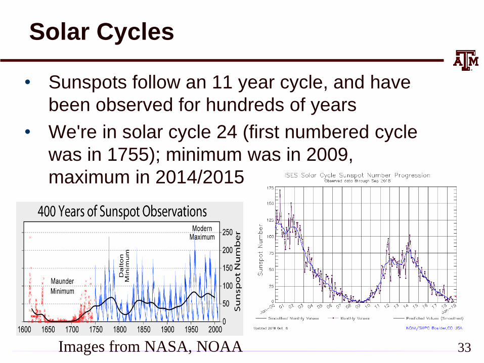
• Sunspots follow an 11 year cycle, and have
been observed for hundreds of years
• We're in solar cycle 24 (first numbered cycle
was in 1755); minimum was in 2009,
maximum in 2014/2015
33Images from NASA, NOAA
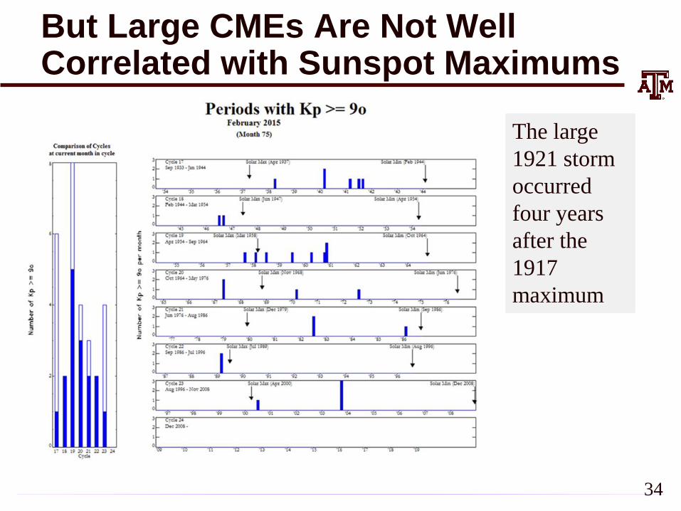
But Large CMEs Are Not Well Correlated with Sunspot Maximums
The large
1921 storm
occurred
four years
after the
1917
maximum
34
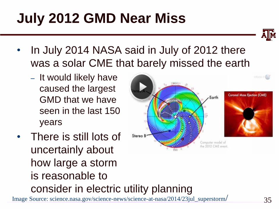
July 2012 GMD Near Miss
• In July 2014 NASA said in July of 2012 there
was a solar CME that barely missed the earth
– It would likely have
caused the largest
GMD that we have
seen in the last 150
years
• There is still lots of
uncertainly about
how large a storm
is reasonable to
consider in electric utility planning Image Source: science.nasa.gov/science-news/science-at-nasa/2014/23jul_superstorm/ 35
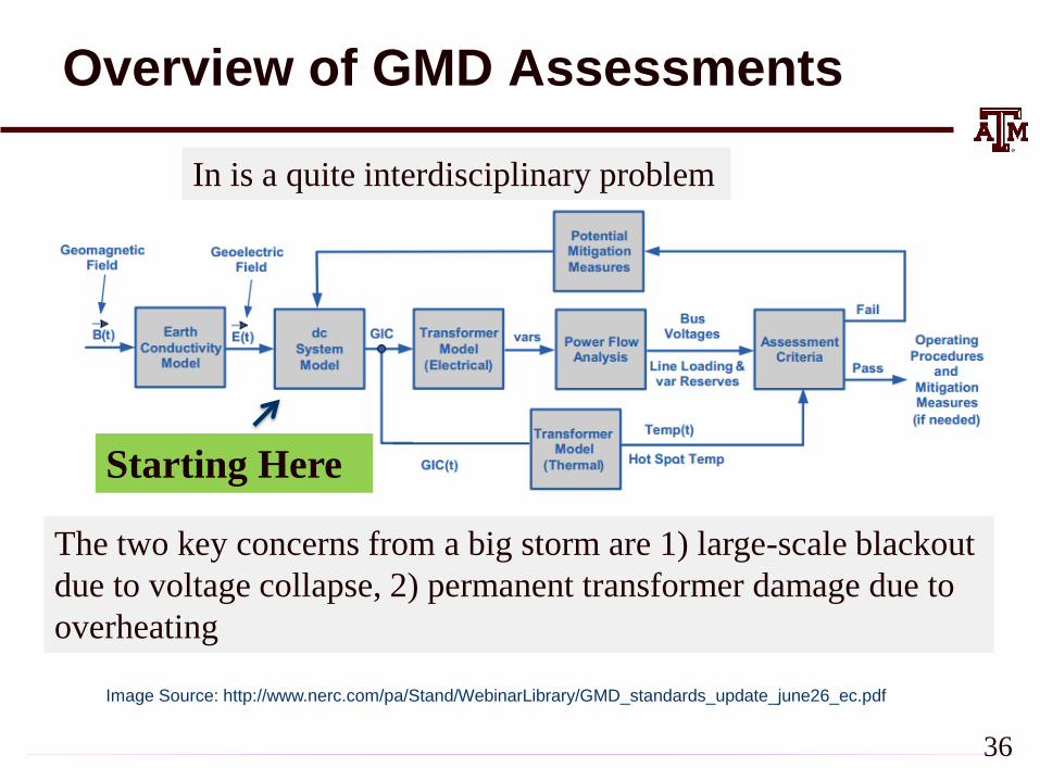
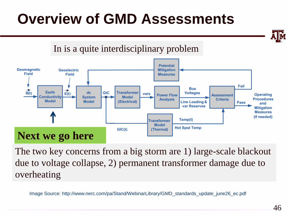
Overview of GMD Assessments
Image Source: http://www.nerc.com/pa/Stand/WebinarLibrary/GMD_standards_update_june26_ec.pdf
The two key concerns from a big storm are 1) large-scale blackout
due to voltage collapse, 2) permanent transformer damage due to
overheating
In is a quite interdisciplinary problem
Starting Here
36
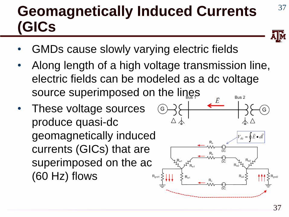
Geomagnetically Induced Currents (GICs
• GMDs cause slowly varying electric fields
• Along length of a high voltage transmission line,
electric fields can be modeled as a dc voltage
source superimposed on the lines
• These voltage sources
produce quasi-dc
geomagnetically induced
currents (GICs) that are
superimposed on the ac
(60 Hz) flows
37
37

GIC Calculations for Large Systems
• With knowledge of the pertinent transmission
system parameters and the GMD-induced line
voltages, the dc bus voltages and flows are found
by solving a linear equation I = G V (or J = G U)
– J and U may be used to emphasize these are dc values,
not the power flow ac values
– The G matrix is similar to the Ybus except 1) it is
augmented to include substation neutrals, and 2) it is just
resistive values (conductances)
• Only depends on resistance, which varies with temperature
– Being a linear equation, superposition holds
– The current vector contains the Norton injections
associated with the GMD-induced line voltages 38
GIC Calculations for Large Systems
• Factoring the sparse G matrix and doing the
forward/backward substitution takes about 1
second for the 60,000 bus Eastern Interconnect
Model
• The current vector (I) depends upon the assumed
electric field along each transmission line
– This requires that substations have correct geo-
coordinates
• With nonuniform fields an exact calculation would
be path dependent, but just a assuming a straight
line path is probably sufficient (given all the other
uncertainties!)39
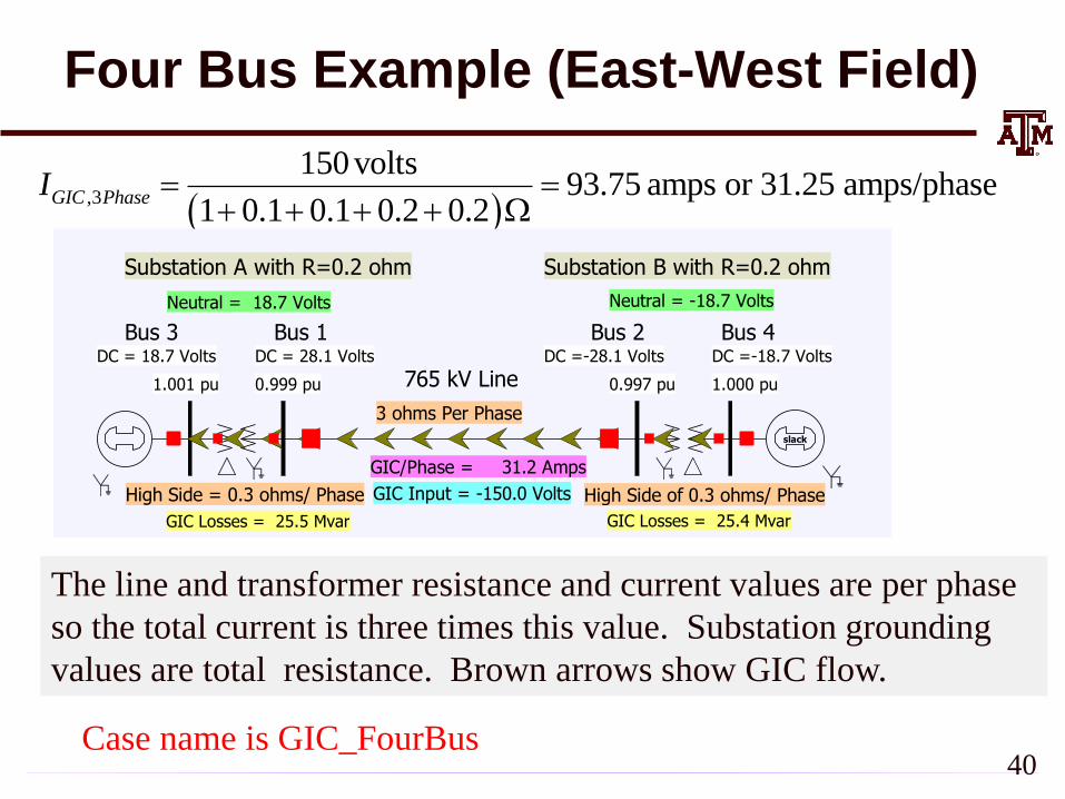
Four Bus Example (East-West Field)
,3
150 volts93.75 amps or 31.25 amps/phase
1 0.1 0.1 0.2 0.2GIC PhaseI
The line and transformer resistance and current values are per phase
so the total current is three times this value. Substation grounding
values are total resistance. Brown arrows show GIC flow.
40
slack
Substation A with R=0.2 ohm Substation B with R=0.2 ohm
765 kV Line
3 ohms Per Phase
High Side of 0.3 ohms/ PhaseHigh Side = 0.3 ohms/ Phase
DC = 28.1 VoltsDC = 18.7 Volts
Bus 1 Bus 4Bus 2Bus 3
Neutral = 18.7 Volts Neutral = -18.7 Volts
DC =-28.1 Volts DC =-18.7 Volts
GIC Losses = 25.5 Mvar GIC Losses = 25.4 Mvar
1.001 pu 0.999 pu 0.997 pu 1.000 pu
GIC/Phase = 31.2 Amps
GIC Input = -150.0 Volts
Case name is GIC_FourBus
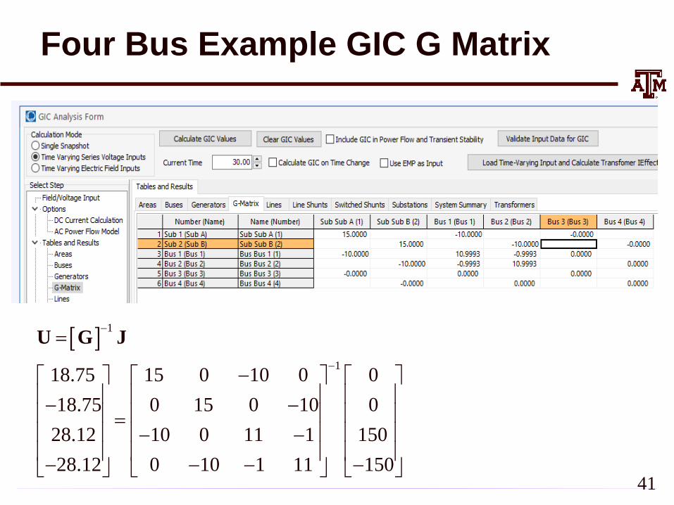
Four Bus Example GIC G Matrix
41
1
118.75 15 0 10 0 0
18.75 0 15 0 10 0
28.12 10 0 11 1 150
28.12 0 10 1 11 150
U G J
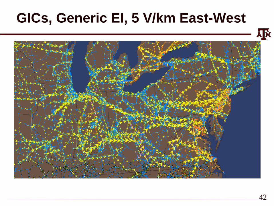
GICs, Generic EI, 5 V/km East-West
42
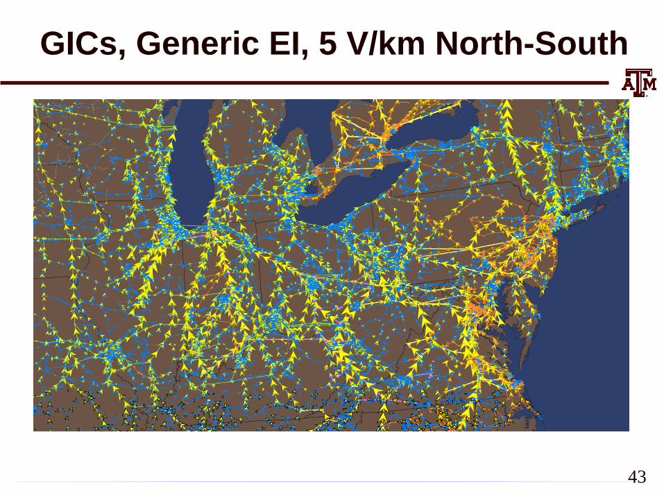
GICs, Generic EI, 5 V/km North-South
43
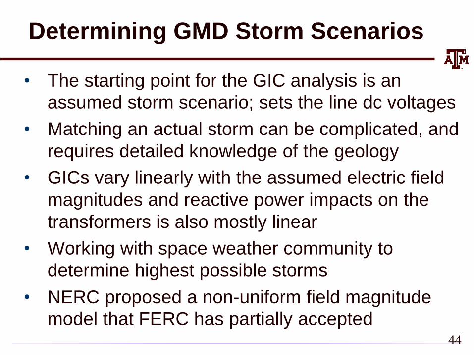
Determining GMD Storm Scenarios
• The starting point for the GIC analysis is an
assumed storm scenario; sets the line dc voltages
• Matching an actual storm can be complicated, and
requires detailed knowledge of the geology
• GICs vary linearly with the assumed electric field
magnitudes and reactive power impacts on the
transformers is also mostly linear
• Working with space weather community to
determine highest possible storms
• NERC proposed a non-uniform field magnitude
model that FERC has partially accepted44
Electric Field Linearity
• If an electric field is assumed to have a uniform
direction everywhere (like with the current NERC
model), then the calculation of the GICs is linear
– The magnitude can be spatially varying
• This allows for very fast computation of the impact of
time-varying functions (like with the NERC event)
• PowerWorld now provides support for loading a
specified time-varying sequence, and quickly
calculating all of the GIC values
45
Overview of GMD Assessments
Image Source: http://www.nerc.com/pa/Stand/WebinarLibrary/GMD_standards_update_june26_ec.pdf
The two key concerns from a big storm are 1) large-scale blackout
due to voltage collapse, 2) permanent transformer damage due to
overheating
In is a quite interdisciplinary problem
Next we go here
46