Embed Size (px)
Citation preview

c©Stanley Chan 2020. All Rights Reserved.
ECE595 / STAT598: Machine Learning ILecture 19 Support Vector Machine: Intro
Spring 2020
Stanley Chan
School of Electrical and Computer EngineeringPurdue University
1 / 32
c©Stanley Chan 2020. All Rights Reserved.
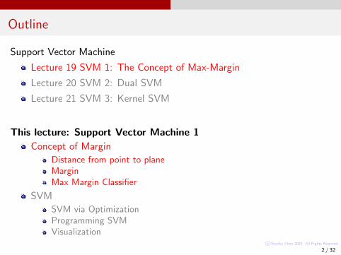
Outline
Support Vector Machine
Lecture 19 SVM 1: The Concept of Max-Margin
Lecture 20 SVM 2: Dual SVM
Lecture 21 SVM 3: Kernel SVM
This lecture: Support Vector Machine 1
Concept of Margin
Distance from point to planeMarginMax Margin Classifier
SVM
SVM via OptimizationProgramming SVMVisualization
2 / 32
c©Stanley Chan 2020. All Rights Reserved.
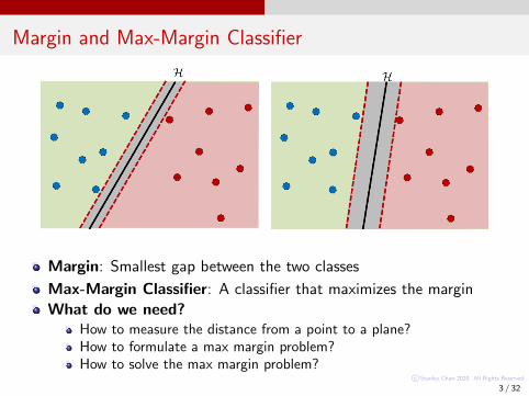
Margin and Max-Margin Classifier
Margin: Smallest gap between the two classes
Max-Margin Classifier: A classifier that maximizes the margin
What do we need?How to measure the distance from a point to a plane?How to formulate a max margin problem?How to solve the max margin problem?
3 / 32
c©Stanley Chan 2020. All Rights Reserved.
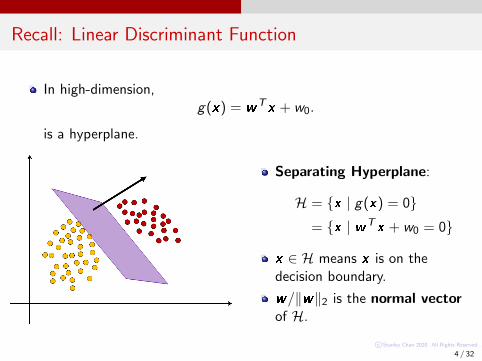
Recall: Linear Discriminant Function
In high-dimension,g(x) = wTx + w0.
is a hyperplane.
Separating Hyperplane:
H = {x | g(x) = 0}= {x | wTx + w0 = 0}
x ∈ H means x is on thedecision boundary.
w/‖w‖2 is the normal vectorof H.
4 / 32
c©Stanley Chan 2020. All Rights Reserved.
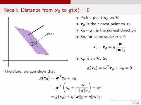
Recall: Distance from x0 to g(x) = 0
Pick a point xp on Hxp is the closest point to x0
x0 − xp is the normal direction
So, for some scalar η > 0,
x0 − xp = ηw
‖w‖2
xp is on H. So
g(xp) = wTxp + w0 = 0Therefore, we can show that
g(x0) = wTx0 + w0
= wT
(xp + η
w
‖w‖2
)+ w0
= g(xp) + η‖w‖2 = η‖w‖2.5 / 32
c©Stanley Chan 2020. All Rights Reserved.
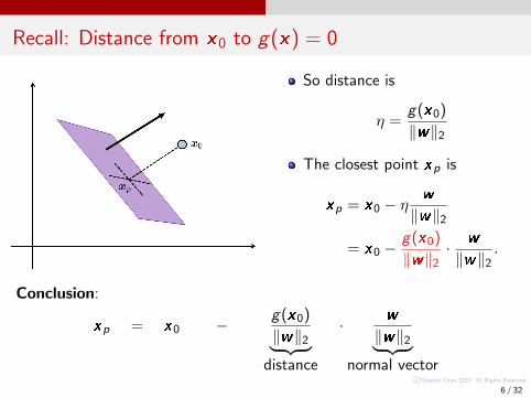
Recall: Distance from x0 to g(x) = 0
So distance is
η =g(x0)
‖w‖2
The closest point xp is
xp = x0 − ηw
‖w‖2
= x0 −g(x0)
‖w‖2· w
‖w‖2.
Conclusion:
xp = x0 − g(x0)
‖w‖2︸ ︷︷ ︸distance
· w
‖w‖2︸ ︷︷ ︸normal vector
6 / 32
c©Stanley Chan 2020. All Rights Reserved.
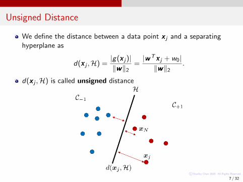
Unsigned Distance
We define the distance between a data point x j and a separatinghyperplane as
d(x j ,H) =|g(x j)|‖w‖2
=|wTx j + w0|‖w‖2
.
d(x j ,H) is called unsigned distance
7 / 32
c©Stanley Chan 2020. All Rights Reserved.
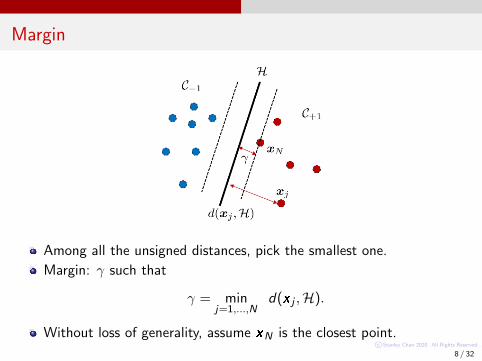
Margin
Among all the unsigned distances, pick the smallest one.
Margin: γ such that
γ = minj=1,...,N
d(x j ,H).
Without loss of generality, assume xN is the closest point.
8 / 32
c©Stanley Chan 2020. All Rights Reserved.
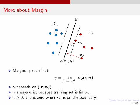
More about Margin
Margin: γ such that
γ = minj=1,...,N
d(x j ,H).
γ depends on (w ,w0).γ always exist because training set is finite.γ ≥ 0, and is zero when xN is on the boundary.
9 / 32
c©Stanley Chan 2020. All Rights Reserved.
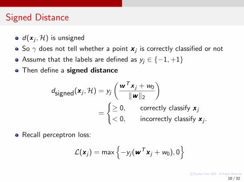
Signed Distance
d(x j ,H) is unsigned
So γ does not tell whether a point x j is correctly classified or not
Assume that the labels are defined as yj ∈ {−1,+1}Then define a signed distance
dsigned(x j ,H) = yj
(wTx j + w0
‖w‖2
)=
{≥ 0, correctly classify x j
< 0, incorrectly classify x j .
Recall perceptron loss:
L(x j) = max{−yj(wTx j + w0), 0
}10 / 32
c©Stanley Chan 2020. All Rights Reserved.
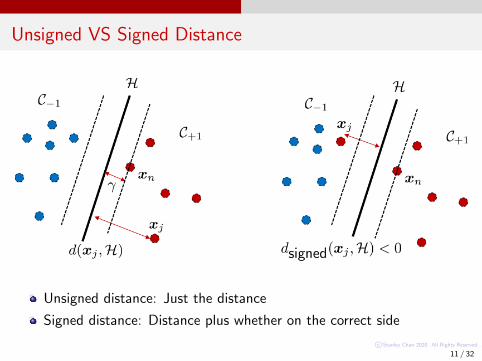
Unsigned VS Signed Distance
Unsigned distance: Just the distance
Signed distance: Distance plus whether on the correct side
11 / 32
c©Stanley Chan 2020. All Rights Reserved.
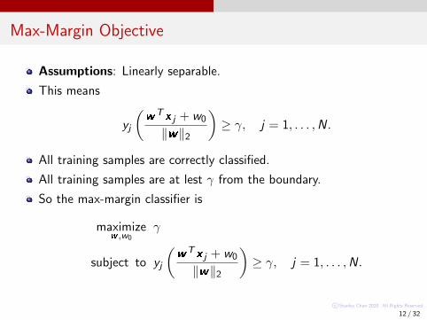
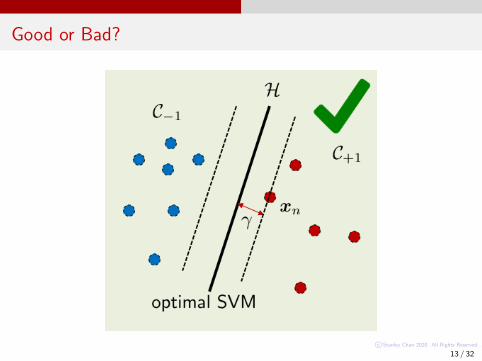
Max-Margin Objective
Assumptions: Linearly separable.
This means
yj
(wTx j + w0
‖w‖2
)≥ γ, j = 1, . . . ,N.
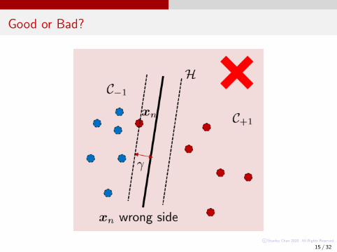
All training samples are correctly classified.
All training samples are at lest γ from the boundary.
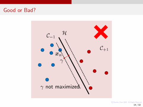
So the max-margin classifier is
maximizew ,w0
γ
subject to yj
(wTx j + w0
‖w‖2
)≥ γ, j = 1, . . . ,N.
12 / 32
c©Stanley Chan 2020. All Rights Reserved.
Good or Bad?
13 / 32
c©Stanley Chan 2020. All Rights Reserved.
Good or Bad?
14 / 32
c©Stanley Chan 2020. All Rights Reserved.
Good or Bad?
15 / 32
c©Stanley Chan 2020. All Rights Reserved.
Outline
Support Vector Machine
Lecture 19 SVM 1: The Concept of Max-Margin
Lecture 20 SVM 2: Dual SVM
Lecture 21 SVM 3: Kernel SVM
This lecture: Support Vector Machine 1
Concept of Margin
Distance from point to planeMarginMax Margin Classifier
SVM
SVM via OptimizationProgramming SVMVisualization
16 / 32
c©Stanley Chan 2020. All Rights Reserved.
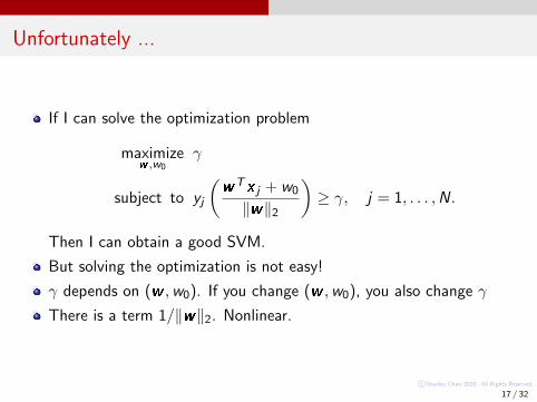
Unfortunately ...
If I can solve the optimization problem
maximizew ,w0
γ
subject to yj
(wTx j + w0
‖w‖2
)≥ γ, j = 1, . . . ,N.
Then I can obtain a good SVM.
But solving the optimization is not easy!
γ depends on (w ,w0). If you change (w ,w0), you also change γ
There is a term 1/‖w‖2. Nonlinear.
17 / 32
c©Stanley Chan 2020. All Rights Reserved.
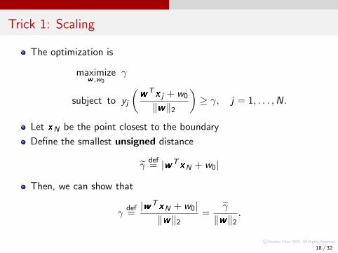
Trick 1: Scaling
The optimization is
maximizew ,w0
γ
subject to yj
(wTx j + w0
‖w‖2
)≥ γ, j = 1, . . . ,N.
Let xN be the point closest to the boundary
Define the smallest unsigned distance
γ̃def= |wTxN + w0|
Then, we can show that
γdef=|wTxN + w0|‖w‖2
=γ̃
‖w‖2.
18 / 32
c©Stanley Chan 2020. All Rights Reserved.
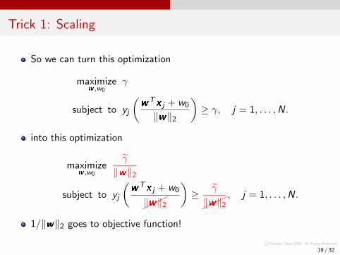
Trick 1: Scaling
So we can turn this optimization
maximizew ,w0
γ
subject to yj
(wTx j + w0
‖w‖2
)≥ γ, j = 1, . . . ,N.
into this optimization
maximizew ,w0
γ̃
‖w‖2
subject to yj
(wTx j + w0
���‖w‖2
)≥ γ̃
���‖w‖2
, j = 1, . . . ,N.
1/‖w‖2 goes to objective function!
19 / 32
c©Stanley Chan 2020. All Rights Reserved.
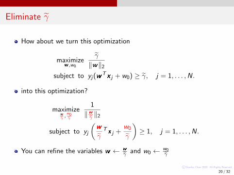
Eliminate γ̃
How about we turn this optimization
maximizew ,w0
γ̃
‖w‖2subject to yj(w
Tx j + w0) ≥ γ̃, j = 1, . . . ,N.
into this optimization?
maximizew
γ̃,w0γ̃
1
‖wγ̃ ‖2
subject to yj
(w
γ̃Tx j +
w0
γ̃
)≥ 1, j = 1, . . . ,N.
You can refine the variables w ← w
γ̃ and w0 ← w0γ̃
20 / 32
c©Stanley Chan 2020. All Rights Reserved.
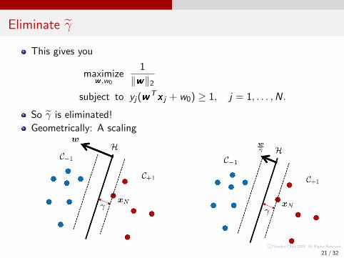
Eliminate γ̃
This gives you
maximizew ,w0
1
‖w‖2subject to yj(w
Tx j + w0) ≥ 1, j = 1, . . . ,N.
So γ̃ is eliminated!
Geometrically: A scaling
21 / 32
c©Stanley Chan 2020. All Rights Reserved.
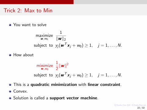
Trick 2: Max to Min
You want to solve
maximizew ,w0
1
‖w‖2subject to yj(w
Tx j + w0) ≥ 1, j = 1, . . . ,N.
How about
minimizew ,w0
1
2‖w‖2
subject to yj(wTx j + w0) ≥ 1, j = 1, . . . ,N.
This is a quadratic minimization with linear constraint.
Convex.
Solution is called a support vector machine.
22 / 32
c©Stanley Chan 2020. All Rights Reserved.
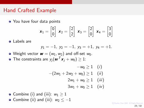
Hand Crafted Example
You have four data points
x1 =
[00
]x2 =
[22
]x3 =
[20
]x4 =
[30
]Labels are
y1 = −1, y2 = −1, y3 = +1, y4 = +1.
Weight vector w = (w1,w2) and off-set w0.
The constraints are yj(wTx j + w0) ≥ 1:
−w0 ≥ 1 (i)
−(2w1 + 2w2 + w0) ≥ 1 (ii)
2w1 + w0 ≥ 1 (iii)
3w1 + w0 ≥ 1 (iv)
Combine (i) and (iii): w1 ≥ 1
Combine (ii) and (iii): w2 ≤ −1
23 / 32
c©Stanley Chan 2020. All Rights Reserved.
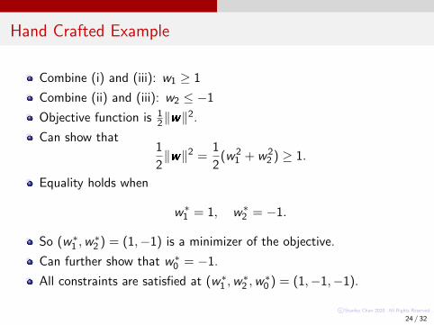
Hand Crafted Example
Combine (i) and (iii): w1 ≥ 1
Combine (ii) and (iii): w2 ≤ −1
Objective function is 12‖w‖
2.
Can show that1
2‖w‖2 =
1
2(w2
1 + w22 ) ≥ 1.
Equality holds when
w∗1 = 1, w∗
2 = −1.
So (w∗1 ,w
∗2 ) = (1,−1) is a minimizer of the objective.
Can further show that w∗0 = −1.
All constraints are satisfied at (w∗1 ,w
∗2 ,w
∗0 ) = (1,−1,−1).
24 / 32
c©Stanley Chan 2020. All Rights Reserved.
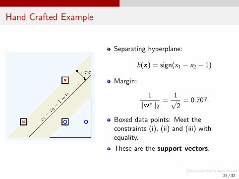
Hand Crafted Example
Separating hyperplane:
h(x) = sign(x1 − x2 − 1)
Margin:
1
‖w∗‖2=
1√2
= 0.707.
Boxed data points: Meet theconstraints (i), (ii) and (iii) withequality.
These are the support vectors.
25 / 32
c©Stanley Chan 2020. All Rights Reserved.
Writing Your SVM
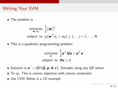
The problem is
minimizew ,w0
1
2‖w‖2
subject to yj(wTx j + w0) ≥ 1, j = 1, . . . ,N.
This is a quadratic programming problem:
minimizeu
1
2uTQu + pTu
subject to Au ≥ c
Solution is u∗ = QP(Q,p,A, c). Solvable using any QP solver.
To us: This is convex objective with convex constraint.
Use CVX! Below is a 1D example.
26 / 32
c©Stanley Chan 2020. All Rights Reserved.
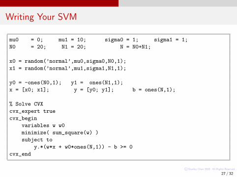
Writing Your SVM
mu0 = 0; mu1 = 10; sigma0 = 1; sigma1 = 1;
N0 = 20; N1 = 20; N = N0+N1;
x0 = random(’normal’,mu0,sigma0,N0,1);
x1 = random(’normal’,mu1,sigma1,N1,1);
y0 = -ones(N0,1); y1 = ones(N1,1);
x = [x0; x1]; y = [y0; y1]; b = ones(N,1);
% Solve CVX
cvx_expert true
cvx_begin
variables w w0
minimize( sum_square(w) )
subject to
y.*(w*x + w0*ones(N,1)) - b >= 0
cvx_end
27 / 32
c©Stanley Chan 2020. All Rights Reserved.
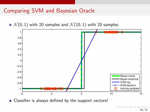
Comparing SVM and Bayesian Oracle
N (0, 1) with 20 samples and N (10, 1) with 20 samples.
−5 0 5 10 15
−1
−0.8
−0.6
−0.4
−0.2
0
0.2
0.4
0.6
0.8
1
Bayes oracle
Bayes empirical
SVM reg
SVM decision
training samples
Classifier is always defined by the support vectors!
28 / 32
c©Stanley Chan 2020. All Rights Reserved.
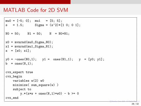
MATLAB Code for 2D SVM
mu0 = [-5; 0]; mu1 = [5; 5];
s = 1.5; Sigma = (s^2)*[1 0; 0 1];
N0 = 50; N1 = 50; N = N0+N1;
x0 = mvnrnd(mu0,Sigma,N0);
x1 = mvnrnd(mu1,Sigma,N1);
x = [x0; x1];
y0 = -ones(N0,1); y1 = ones(N1,1); y = [y0; y1];
b = ones(N,1);
cvx_expert true
cvx_begin
variables w(2) w0
minimize( sum_square(w) )
subject to
y.*(x*w + ones(N,1)*w0) - b >= 0
cvx_end
29 / 32
c©Stanley Chan 2020. All Rights Reserved.
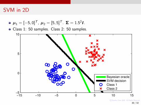
SVM in 2D
µ1 = [−5, 0]T , µ2 = [5, 5]T . Σ = 1.52I .
Class 1: 50 samples. Class 2: 50 samples.
−15 −10 −5 0 5 10 15−5
0
5
10
Bayesian oracle
SVM decision
Class 1
Class 2
30 / 32
c©Stanley Chan 2020. All Rights Reserved.
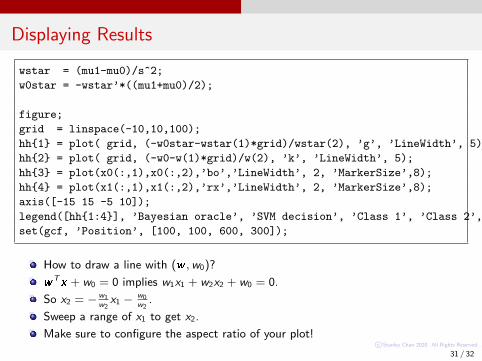
Displaying Results
wstar = (mu1-mu0)/s^2;
w0star = -wstar’*((mu1+mu0)/2);
figure;
grid = linspace(-10,10,100);
hh{1} = plot( grid, (-w0star-wstar(1)*grid)/wstar(2), ’g’, ’LineWidth’, 5); hold on;
hh{2} = plot( grid, (-w0-w(1)*grid)/w(2), ’k’, ’LineWidth’, 5);
hh{3} = plot(x0(:,1),x0(:,2),’bo’,’LineWidth’, 2, ’MarkerSize’,8);
hh{4} = plot(x1(:,1),x1(:,2),’rx’,’LineWidth’, 2, ’MarkerSize’,8);
axis([-15 15 -5 10]);
legend([hh{1:4}], ’Bayesian oracle’, ’SVM decision’, ’Class 1’, ’Class 2’, ’Location’, ’SE’);
set(gcf, ’Position’, [100, 100, 600, 300]);
How to draw a line with (w ,w0)?
wTx + w0 = 0 implies w1x1 + w2x2 + w0 = 0.
So x2 = −w1w2x1 − w0
w2.
Sweep a range of x1 to get x2.
Make sure to configure the aspect ratio of your plot!
31 / 32
c©Stanley Chan 2020. All Rights Reserved.
Reading List
Support Vector Machine
Mustafa, Learning from Data, e-Chapter
Duda-Hart-Stork, Pattern Classification, Chapter 5.5
Chris Bishop, Pattern Recognition, Chapter 7.1
UCSD Statistical Learninghttp://www.svcl.ucsd.edu/courses/ece271B-F09/
32 / 32