ECE295,  Data  Assimila0on  and  Inverse  Problems,  Spring  2014  •  Classes  2  April,  Intro;  Linear  discrete  Inverse  problems  (Aster  Ch  1)  Slides  9  April,  SVD  (Aster  ch  2  and  3)  Slides  16  April,  RegularizaFon  (ch  4)  Slides  23  April,  Sparse  methods  (ch  7.2-­‐7.3)  Slides  30  April,  Bayesian  methods  (ch  11)  7  May,  Markov  Chain  Monte  Carlo  (download  from  Mark  Steyvers  )  14  May,  (Caglar  Yardim)  IntroducFon  to  sequenFal  Bayesian  methods  21  May,  Kalman  28  May,  EKF,UKF,EnKF  4  June,  PF    Homework:  You  can  use  any  programming  language,  matlab  is  the  most  obvious,  some  MathemaFca  or  Python  could  be  fun!    Hw  1:  Download  the  matlab  codes  for  the  book  (cd_5.3)  from  this  website  h`p://www.ees.nmt.edu/outside/courses/GEOP529_book.html.  Run  the  3  examples  for  chapter  2.  Come  to  class  with  one  quesFon  about  the  examples.  Due  9  April.  hw  2,  16  April,  SVD  ;  read  chapter  one  of  Steyvers  notes,  hw3,  23  April,  RegularizaFon  hw4,  30  April,  Sparse  problems  hw5,  7  May,  Monte  Carlo  integraFon  hw6,  14  May,  Metropolis  algorithm  (Steyvers  Ch  2.4.1-­‐2.4.5);  Metropolis-­‐HasFngs  algorithm,  (Steyvers  Ch  2.6.1-­‐2.6.3).  

Example  7.4  

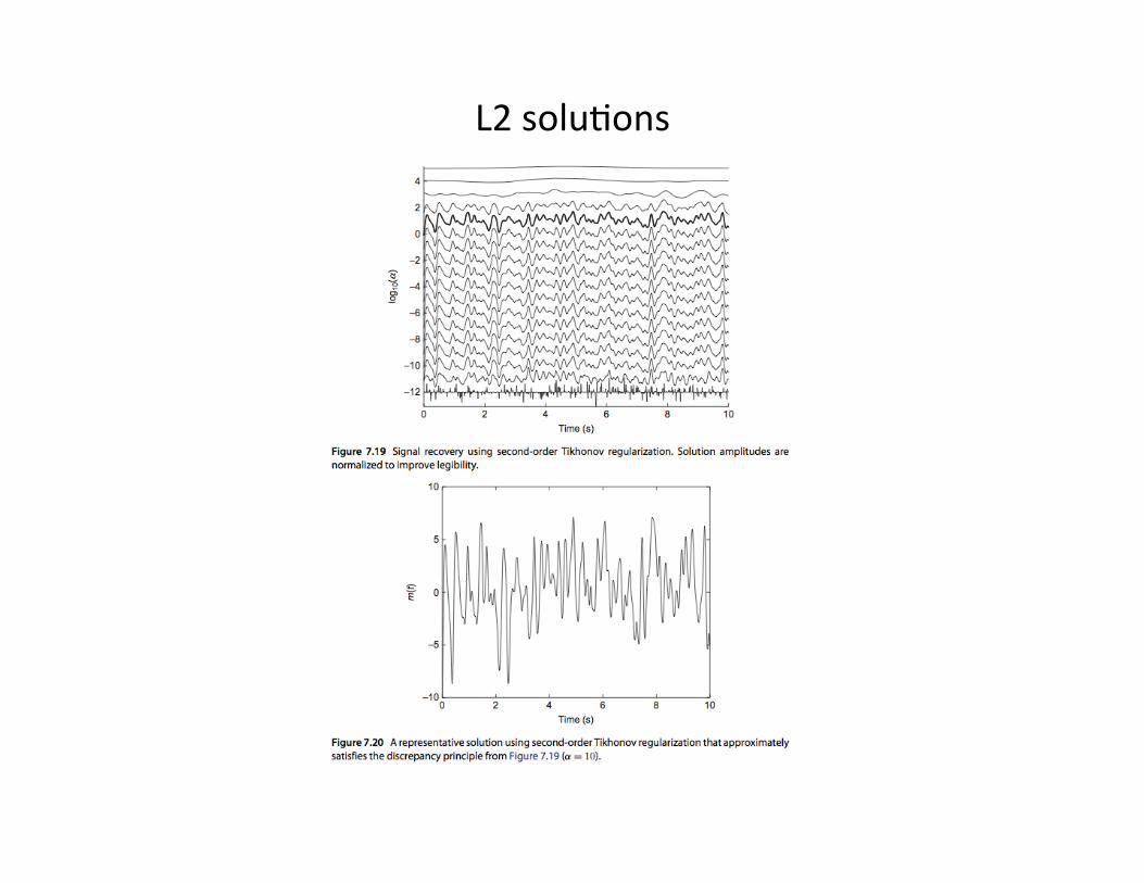
L2  soluFons  

Problem  7.4  

d1000 x1 =W1000 x1000m1000 x1 + n1000 x1q100 x1 =G100 x1000d1000 x1 = G100 x1000W1000 x1000m1000 x1 + n '1000 x1

L1  soluFons  

277

Generating samples from an arbitrary posterior PDF

The rejection method

278

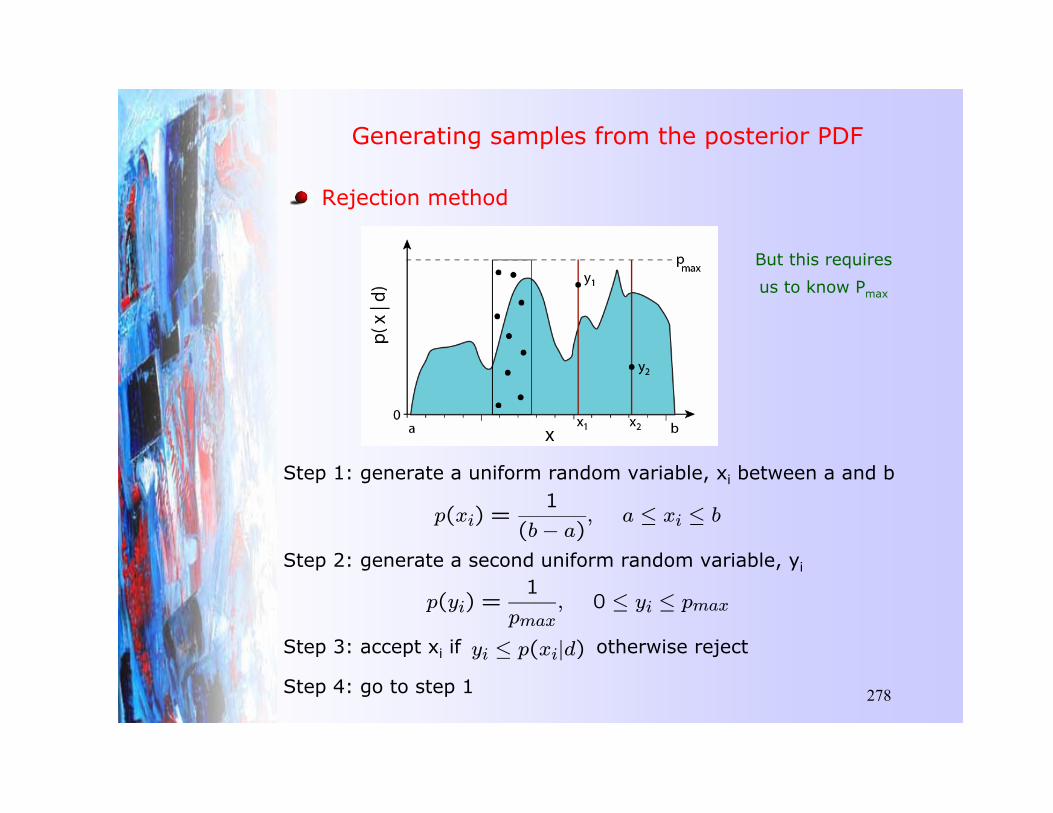
Generating samples from the posterior PDF

Rejection method

Step 1: generate a uniform random variable, xi between a and b

p(xi) =1

(bc a), a w xi w b

Step 2: generate a second uniform random variable, yi

p(yi) =1

pmax, 0 w yi w pmax

Step 3: accept xi if otherwise rejectyi w p(xi|d)

Step 4: go to step 1

But this requires us to know Pmax

286

Monte Carlo integration

Consider any integral of the form

I =Z

Mf(m)p(m|d)dm

I |NsX

i=1

f(mi)p(mi|d)h(mi)

Given a set of samples mi (i=,...,Ns) with sampling density h(mi), theMonte Carlo approximation to I is given by

If the sampling density is proportional to p(mi | d) then,

h(m) = Ns × p(m|d)

� I | 1

Ns

NsX

i=1

f(mi)

The variance of the f(mi) values gives the numerical integration error in I

Only need to know p(m | d) to a

multiplicative constant

287

Example: Monte Carlo integration

h(m) =Ns

A

I =Z

Af(m)dm

f(m) =

(1 m inside circle0 otherwise

Finding the area of a circle by throwing darts

I |1

Ns

NSX

i=1

f(mi)

| Number of points inside the circle

Total number of points

288

Monte Carlo integration

We have

I =Z

Mf(m)p(m|d)dm |

NsX

i=1

f(mi)p(mi|d)h(mi)

|1

Ns

NsX

i=1

f(mi)

The variance in this estimate is given by

~2I =1

Ns

�!�

!�1

N2s

NsX

i=1

f2(mi)c

�

# 1

Ns

NsX

i=1

f(mi)

�

$2�!

!�

In principal any sampling density h(m) can be used but the convergence rate will be fastest when h(m) � p(m | d).

As the number of samples, Ns, grows the error in the numerical estimate will decrease with the square root of Ns.

What useful integrals should one calculate using samples distributed according to the posterior p(m | d )?

To carry out MC integration of the posterior we ONLY NEED to be able to evaluate the integrand up to a multiplicative constant.

The  volume  of  a  N-­‐dim  cube  2^N    For  N=2  3.14/2^2=3/4    For  N=10  3.14^5/120/2^10=2/1000    This  will  be  hard!  

Probabilistic inference

Bayes theorem and all that....

Books

250

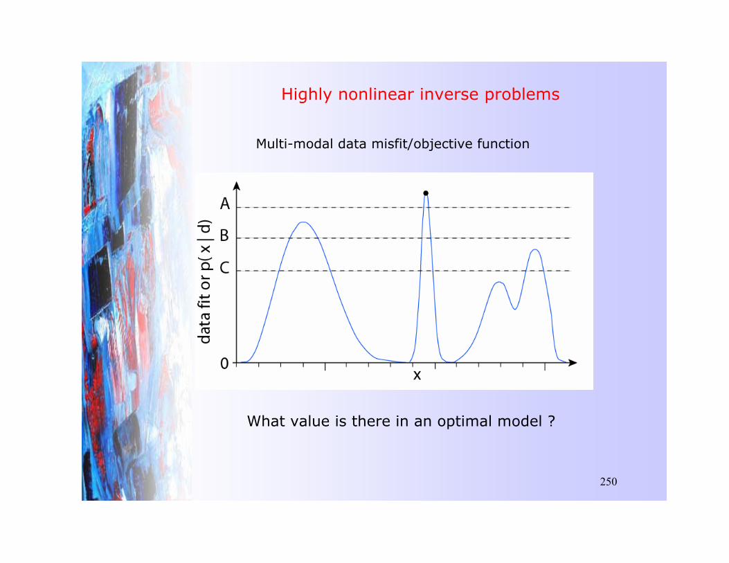
Highly nonlinear inverse problems

Multi-modal data misfit/objective function

What value is there in an optimal model ?

251

Probabilistic inference: History

Pr(x : a w x w b) =Z b

ap(x)dx

We have already met the concept of using a probability density function p(x) to describe the state of a random variable.

In the probabilistic (or Bayesian) approach, probabilities are also used to describe inferences (or degrees of belief) about x even if x itself is not a random variable.

Mass of Saturn (Laplace 1812)p(M

|data,I)

Laplace (1812) rediscovered the work of Bayes (1763), and used it to constrain the mass of Saturn. In 150 years the estimate changed by only 0.63% !

But Laplace died in 1827 and then the arguments started...

Z �

c�p(x)dx= 1

252

Bayesian or Frequentist: the arguments

Mass of Saturn

Some thought that using probabilities to describe degrees of belief was too subjective and so they redefined probability as the long run relative frequency of a random event. This became the Frequentist approach.

To estimate the mass of Saturn the frequentist has to relate the mass to the data through a statistic. Since the data contain `random’ noise probability theory can be applied to the statistic (which becomes the random variable !). This gave birth to the field of statistics !

But how to choose the statistic ?

`.. a plethora of tests and procedures without any clear underlying rationale’(D. S. Sivia)

`Bayesian is subjective and requires too many guesses’

A. Frequentist

`Frequentist is subjective, but BI can solve problems more completely’

A. Bayesian

For a discussion see Sivia (2005, pp 8-11).

Data Analysis: A Bayesian Tutorial’ 2nd Ed. D. S. Sivia with J. Skilling, O.U.P. (2005)

253

Probability theory: Joint probability density functions

Joint PDF of x and y

p(x, y)

p(x, y) = p(x)× p(y)

If x and y are independent their joint PDF is separable

p(x)

A PDF for variable x

Probability is proportional to area under the curve or surface

254

p(y|x)

Probability theory: Conditional probability density functions

Joint PDF of x and y

p(x|y)p(x, y)

Conditional PDFs

p(x, y) = p(x|y)× p(y)Relationship between joint and conditional PDFs

“The PDF of x given a value for y”“The PDF of x and y taken together”

255

Probability theory: Marginal probability density functions

Marginal PDFs

p(x, y) = p(x|y)× p(y)Relationship between joint, conditional and marginal PDFs

p(y) =Zp(x, y)dx

p(x) =Zp(x, y)dy

A marginal PDF is a summation of probabilities

256

Prior probability density functions

What we know from previous experiments, or what we guess...

Beware: there is no such thing as a non-informative prior

p(x) = k exp

(

c(xc xo)2

2~2

)

p(m) = k exp

½c1

2(mcmo)

TCc1m (mcmo)

¾

p(x)dx= p(y)dy

p(x) = C

p(y) = p(x)dx

dy

p(x2) =C

2x

Beware: there is no such thing as a non-informative prior

As A � � this is not proper !

257

Likelihood functions

The likelihood that the data would have occurred for a given model

Maximizing likelihoods is what Frequentists do. It is what we did earlier.

p(di|x) = exp

(

c(xc xo,i)2

2~2i

)

p(d|m) = exp

½c12(dcGm)TCc1D (dcGm)

¾

maxm

p(d|m) = minm

c ln(p(d|m))

= minm

(dcGm)TCc1D (dcGm)

Maximizing the likelihood = minimizing the data prediction error

258

Bayes’ theorem

p(m|d, I) � p(d|m, I)× p(m|I)

Conditional PDFsBayes’ rule (1763)

Posterior probability density � Likelihood x Prior probability density

All information is expressed in terms of probability density functions

1702-1761

What is known before the data are collected

Measuring fit to data

What is known after the data are collected

Assumptions

model parametersdata

259

Example: Measuring the mass of an object

If we have an object whose mass, m, we which to determine. Before we collect any data we believe that its mass is approximately 10.0 ± 1Pg. In probabilistic terms we could represent this as a Gaussian prior distribution

p(m|d) � ec12(mc10.96)

2

1/5

p(m) =1S2|ec

12(mc10.0)

2

Suppose a measurement is taken and a value 11.2 P g is obtained, and the measuring device is believed to give Gaussian errors with mean 0 and V = 0.5 P g.Then the likelihood function can be written

p(d|m) =1

0.5S2|ec2(mc11.2)

2

The posterior PDF becomes a Gaussian centred at the value of 10.96 P g with standard deviation V= (1/5)1/2 ~ 0.45.

p(m|d) =1

|ec

12(mc10.0)

2c2(mc11.2)2

prior

Likelihood

Posterior

260

Example: Measuring the mass of an object

p(d|m) � exp½c12(dcGm)TCc1d (dcGm)

¾

� exp½c12[(dcGm)TCc1d (dcGm) + (mcmo)

TCc1m (mcmo)]

¾

The more accurate new data has changed the estimate of m and decreased its uncertainty

For the general linear inverse problem we would have

p(m) � exp½c1

2(mcmo)

TCc1m (mcmo)

¾Prior:

Likelihood:

Posterior PDF

One data point problem

261

The biased coin problem

Suppose we have a suspicious coin and we want to know if it is biased or not ?

Let D be the probability that we get a head.

D = 1 : means we always get a head.D = 0 : means we always get a tail.D = 0.5 : means equal likelihood of head or tail.

We can collect data by tossing the coin many times

We seek a probability density function for D given the data

p(n|d, I) � p(d|n, I)× p(n|I)

Posterior PDF � Likelihood x Prior PDF

{H,T, T,H, . . .}

262

The biased coin problem

p(n|d, I) � p(d|n, I)× p(n|I)Posterior PDF � Likelihood x Prior PDF

What is the prior PDF for D ?

Let us assume that it is uniform

p(n|I) = 1, 0 w n w 1

What is the Likelihood function ?

p(d|n, I) � nR(1c n)NcR

The probability of observing R heads out of N coin tosses is

263

The biased coin problemWe have the posterior PDF for D given the data and our prior PDF

p(n|d, I) � nR(1c n)NcR

After N coin tosses let R = number of heads observed. Then we Can plot the probability density for p(D | d) as data are collected

Number

of data

264

The biased coin problem

p(n|d, I) � nR(1c n)NcR

Number

of data

265

The biased coin problem

But what if three people had different opinions about the coin prior to collecting the data ?

Dr. Blue knows nothing about the coin.

p(d|n, I) � nR(1c n)NcR

Dr. Red thinks the coin is either highly biased to heads or tails.

Dr. Green thinks the coin is likely to be almost fair.

266

The biased coin problem

Number

of data

268

How to choose a prior ?

An often quoted weakness of Bayesian inversion is the subjectiveness of the prior.

There is no such thing as a non-informative prior !

If we know that x > 0 and that E{x} = P. What is an appropriate prior p(x) ?

A solution is to choose the prior p(x) that maximizes entropy subject to satisfying the constraints. Using calculus of variations we get

H(X) =Z �

c�p(x) ln p(x)dx Entropy

p(x) =1

yecx/y, x x 0

269

In the Bayesian treatment, all inferences are expressed in terms ofprobabilities.

Bayes’ theorem tells us how to combine a priori information with theinformation provided by the data, and all are expressed as PDFs.

All Bayesian inference is relative. We always compare what we knowafter the data are collected to what we know before the data are collected. In practice this means comparing the a posteriori PDF with the a priori PDF.

Bayesians argue that this is just a formalization of logical inference.

Criticisms are that non-informative prior’s do not exist, and hencewe introduce information if prior’s are assumed for convenience.

The general framework is appealing but can not usually be appliedwhen the number of unknowns is >= 103.

Recap: Probabilistic inference

270

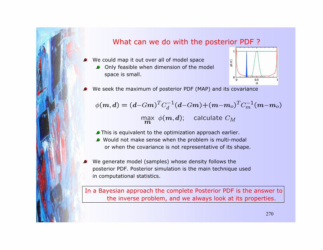
What can we do with the posterior PDF ?

We could map it out over all of model spaceOnly feasible when dimension of the model space is small.

We seek the maximum of posterior PDF (MAP) and its covariance

This is equivalent to the optimization approach earlier.Would not make sense when the problem is multi-modalor when the covariance is not representative of its shape.

We generate model (samples) whose density follows the posterior PDF. Posterior simulation is the main technique used in computational statistics.

�(m,d) = (dcGm)TCc1d (dcGm)+(mcmo)TCc1m (mcmo)

maxm

�(m,d); calculate CM

In a Bayesian approach the complete Posterior PDF is the answer tothe inverse problem, and we always look at its properties.