ECE 5582 Computer Vision · Perspective Projection Examples Perspective projection is a simplification of real world image formation Lens characteristics are not considered Perspective

Spring 2020: Venu: Haag 312, Time: M/W 4-5:15pm

ECE 5582 Computer VisionLec 03: Image Formation - Geometry

Zhu LiDept of CSEE, UMKC

Office: FH560E, Email: [email protected], Ph: x 2346.http://l.web.umkc.edu/lizhu

Z. Li: ECE 5582 Computer Vision, 2020 p.1

slides created with WPS Office Linux and EqualX LaTex equation editor

Outline

Recap of Lec 02 Projection Geometry of Image Formation Homography Summary


Outline



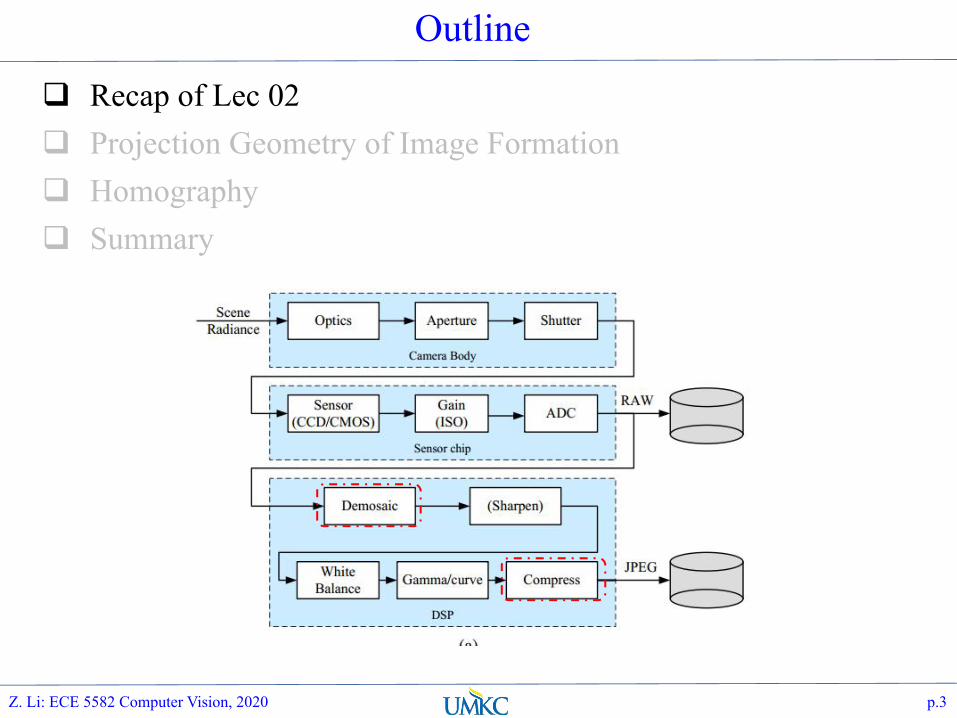
Demosaicing

Demosaicing in deep learning era: [5] Nai-Sheng Syu*, Yu-Sheng Chen*, Yung-Yu Chuang , “Learning Deep Convolutional

Networks for Demosaicing”.


handcrafted

deep learning based

DMCNN

Similar to our ICME work, residual learning blocks with BN and SE

Good performance:


paras' network [6] fordark image denoising and demosaic

HSV Color Model

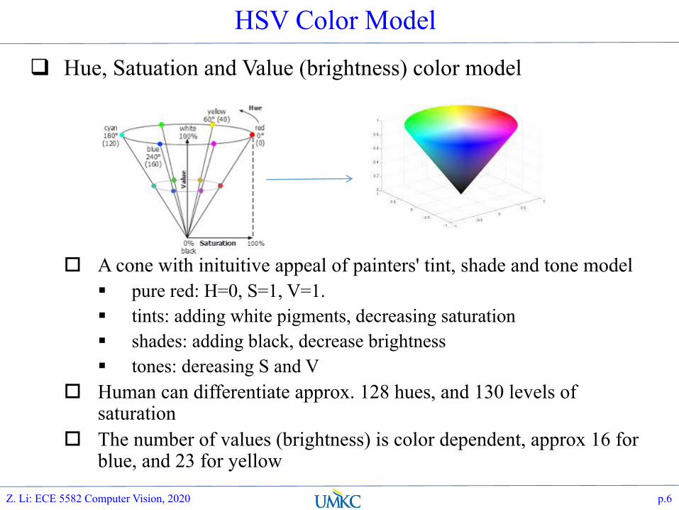
Hue, Satuation and Value (brightness) color model

A cone with inituitive appeal of painters' tint, shade and tone model pure red: H=0, S=1, V=1. tints: adding white pigments, decreasing saturation shades: adding black, decrease brightness tones: dereasing S and V

Human can differentiate approx. 128 hues, and 130 levels of saturation

The number of values (brightness) is color dependent, approx 16 for blue, and 23 for yellow


MPEG-7 Scalable Color Descriptor

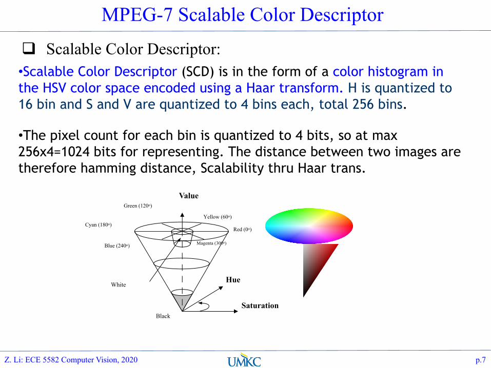
Scalable Color Descriptor:•Scalable Color Descriptor (SCD) is in the form of a color histogram in the HSV color space encoded using a Haar transform. H is quantized to 16 bin and S and V are quantized to 4 bins each, total 256 bins.

•The pixel count for each bin is quantized to 4 bits, so at max 256x4=1024 bits for representing. The distance between two images are therefore hamming distance, Scalability thru Haar trans.

Saturation

Hue

Value

Red (0o)

Yellow (60o)

Green (120o)

Cyan (180o)

Blue (240o) Magenta (300o)

Black

White

p.7Z. Li: ECE 5582 Computer Vision, 2020

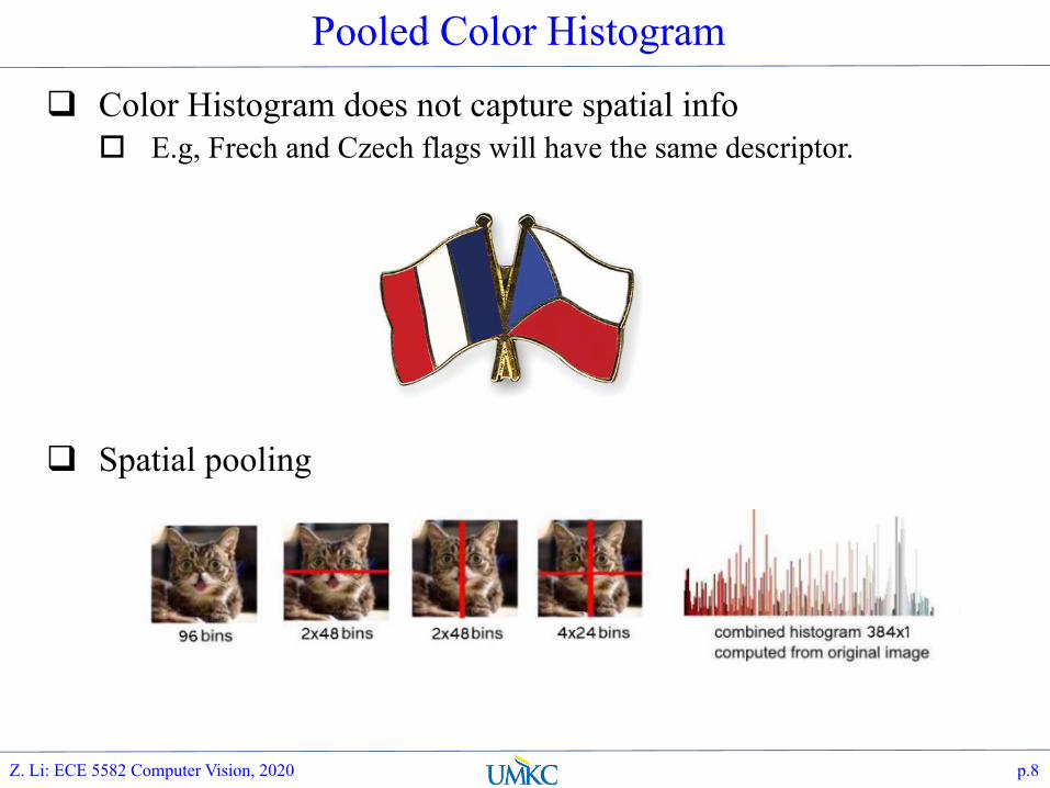
Pooled Color Histogram

Color Histogram does not capture spatial info E.g, Frech and Czech flags will have the same descriptor.

Spatial pooling


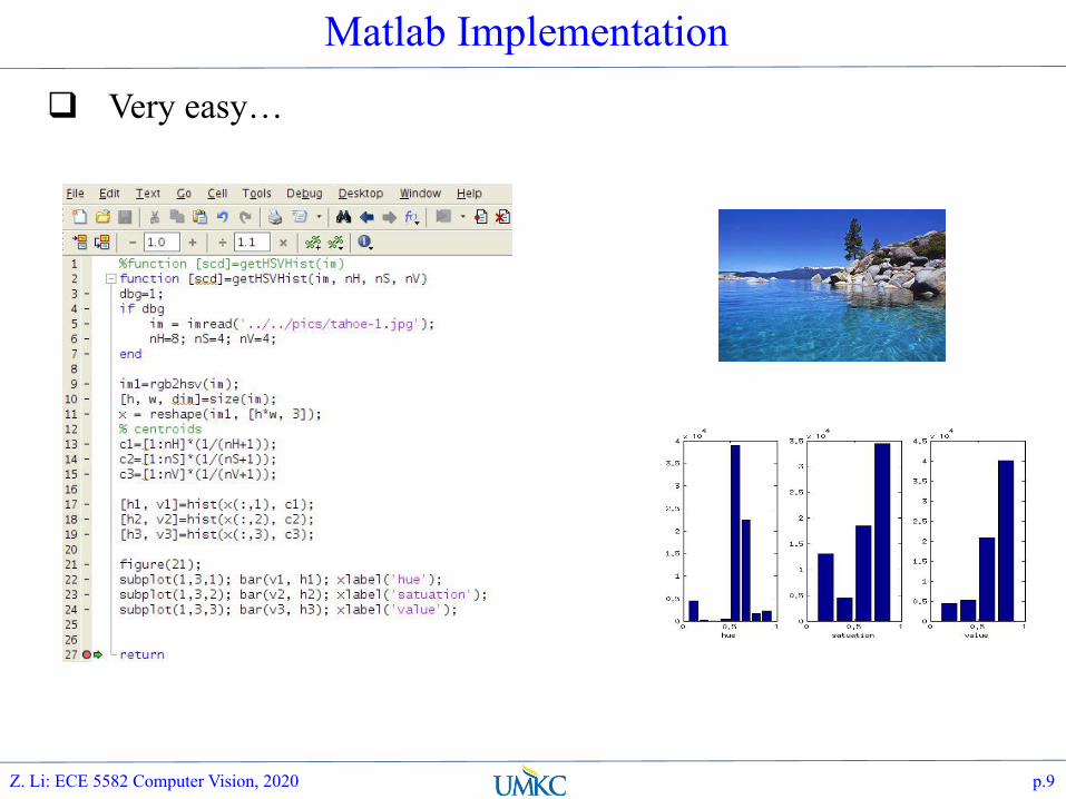
Matlab Implementation

Very easy…


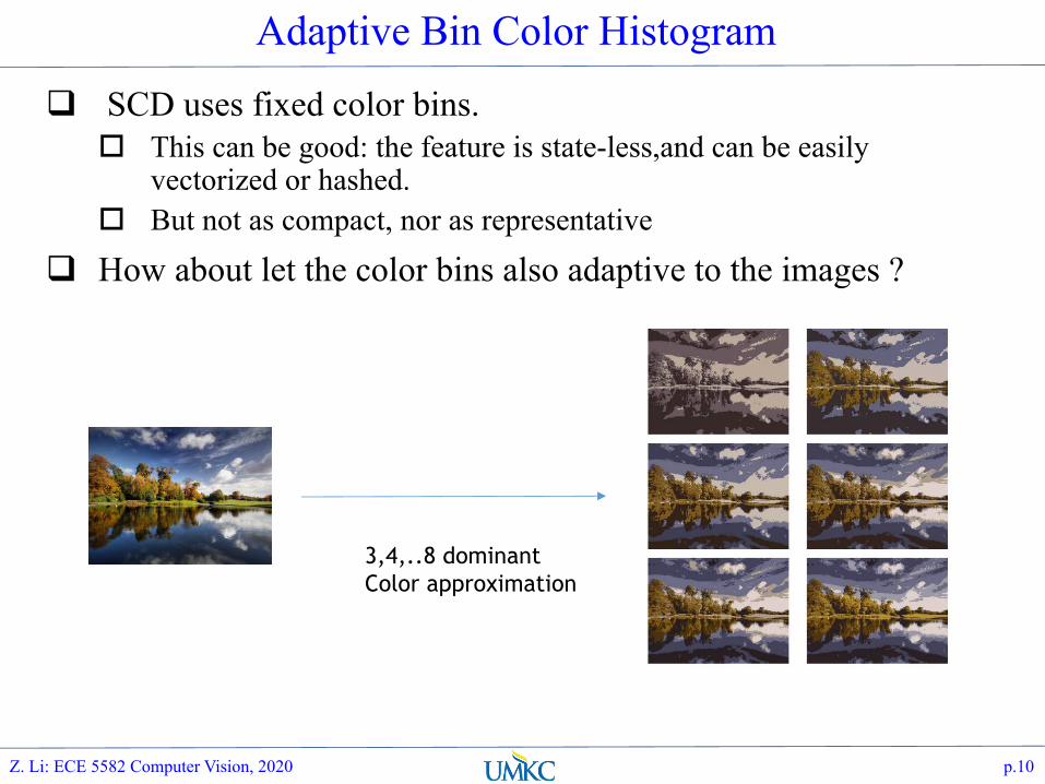
Adaptive Bin Color Histogram

SCD uses fixed color bins. This can be good: the feature is state-less,and can be easily

vectorized or hashed. But not as compact, nor as representative

How about let the color bins also adaptive to the images ?


3,4,..8 dominantColor approximation

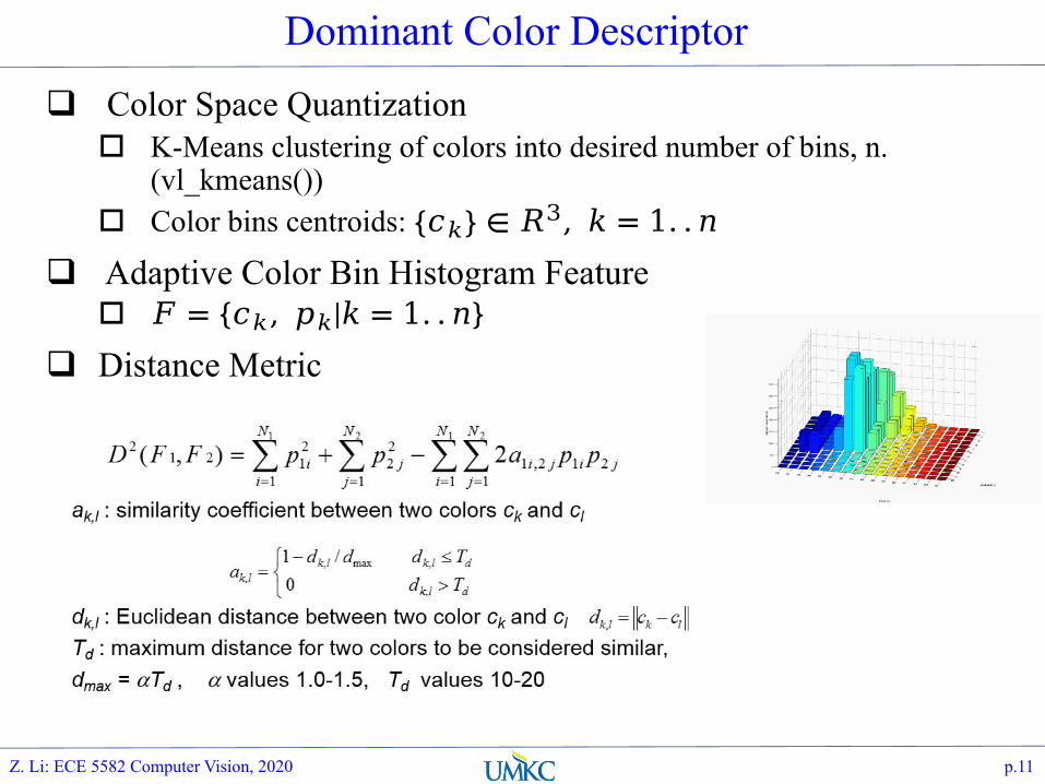
Dominant Color Descriptor

Color Space Quantization K-Means clustering of colors into desired number of bins, n.

(vl_kmeans()) Color bins centroids: �� ∈ ��, � = 1. . �

Adaptive Color Bin Histogram Feature � = ��, ��|� = 1. . ��

Distance Metric


Matlab Implementation

Again, rather easy with Matlab:


Outline



Pinhole Camera Model

Aperture : avoid ambiguity on image plane

Pinhole Camera model:


focal length: f

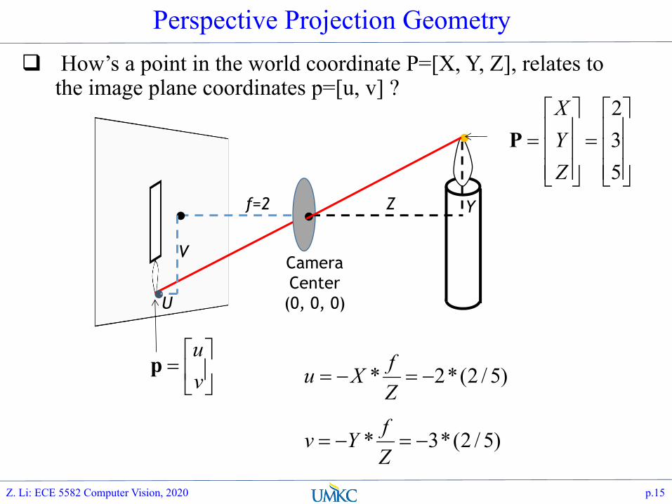
Perspective Projection Geometry How’s a point in the world coordinate P=[X, Y, Z], relates to

the image plane coordinates p=[u, v] ?


Camera Center

(0, 0, 0)

úúú

û

ù

êêê

ë

é=

úúú

û

ù

êêê

ë

é=

532

ZYX

P.

.. f=2 Z Y

úû

ùêë

é=

vu

p

.V

U

)5/2(*2* -=-=ZfXu

)5/2(*3* -=-=ZfYv

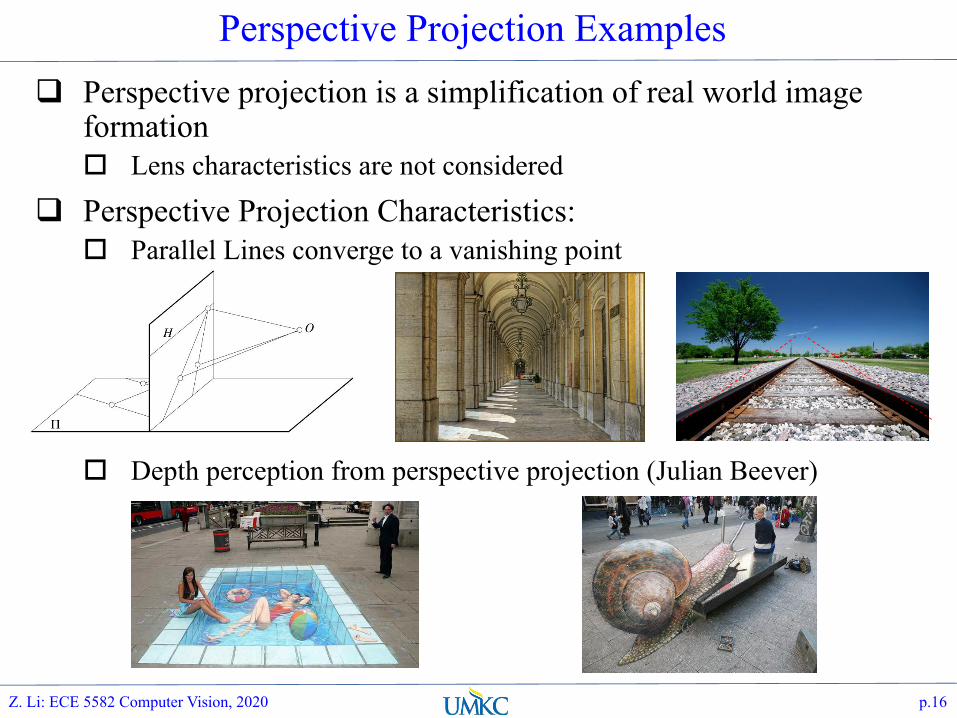
Perspective Projection Examples Perspective projection is a simplification of real world image

formation Lens characteristics are not considered

Perspective Projection Characteristics: Parallel Lines converge to a vanishing point

Depth perception from perspective projection (Julian Beever)


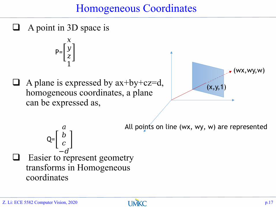
Homogeneous Coordinates

A point in 3D space is

A plane is expressed by ax+by+cz=d, homogeneous coordinates, a plane can be expressed as,

Easier to represent geometry transforms in Homogeneous coordinates


P=��1�

Q=��−��

(x,y,1)

(wx,wy,w)

All points on line (wx, wy, w) are represented

Intrinsic Parameters: focal length


[ ]X0IKx =úúúú

û

ù

êêêê

ë

é

úúú

û

ù

êêê

ë

é=

úúú

û

ù

êêê

ë

é

10100000000

1zyx

ff

vu

w

K

Slide Credit: GaTech Computer Vision class, 2015.

Intrinsic Assumptions• Unit aspect ratio• Optical center at (0,0)• No skew of pixels

Extrinsic Assumptions• No rotation• Camera at (0,0,0)

X

x

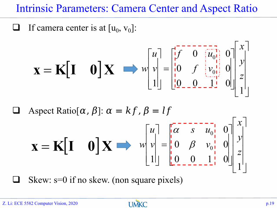
Intrinsic Parameters: Camera Center and Aspect Ratio

If camera center is at [u0, v0]:

Aspect Ratio[�,�]: � = �X,� = �X

Skew: s=0 if no skew. (non square pixels)


[ ]X0IKx =úúúú

û

ù

êêêê

ë

é

úúú

û

ù

êêê

ë

é=

úúú

û

ù

êêê

ë

é

101000000

10

0

zyx

vfuf

vu

w

[ ]X0IKx =úúúú

û

ù

êêêê

ë

é

úúú

û

ù

êêê

ë

é=

úúú

û

ù

êêê

ë

é

10100000

10

0

zyx

vus

vu

w ba

3D Rotation

Rotate along axis, the order matters


� = ��

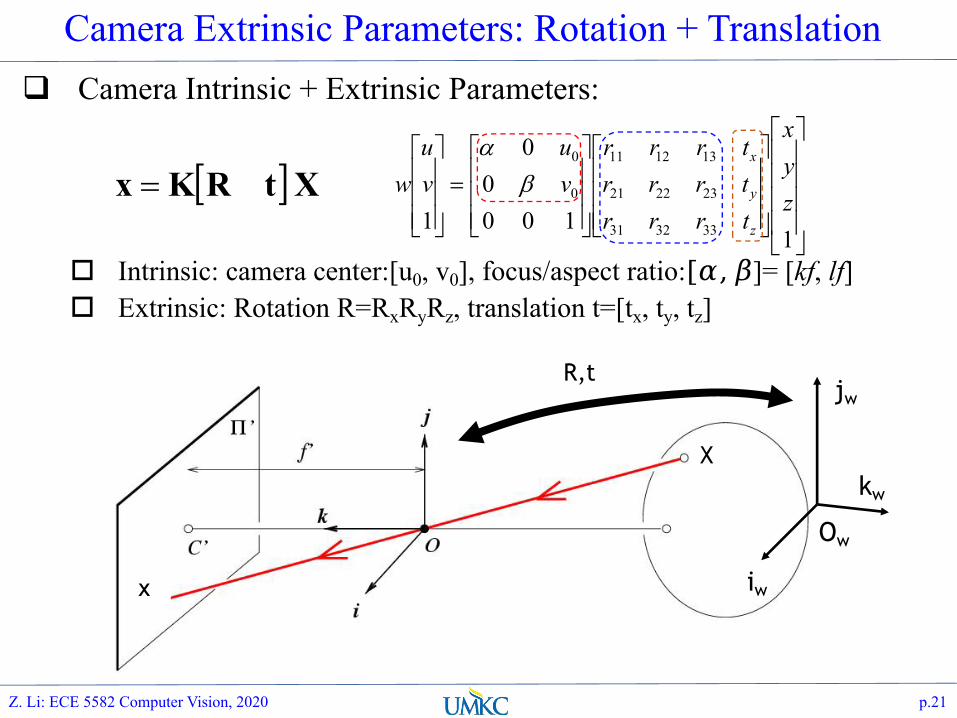
Camera Extrinsic Parameters: Rotation + Translation Camera Intrinsic + Extrinsic Parameters:

Intrinsic: camera center:[u0, v0], focus/aspect ratio:[�,�]= [kf, lf] Extrinsic: Rotation R=RxRyRz, translation t=[tx, ty, tz]


[ ]XtRKx =úúúú

û

ù

êêêê

ë

é

úúú

û

ù

êêê

ë

é

úúú

û

ù

êêê

ë

é=

úúú

û

ù

êêê

ë

é

1100

00

1 333231

232221

131211

0

0

zyx

trrrtrrrtrrr

vu

vu

w

z

y

x

ba

Ow

iw

kw

jwR,t

X

x

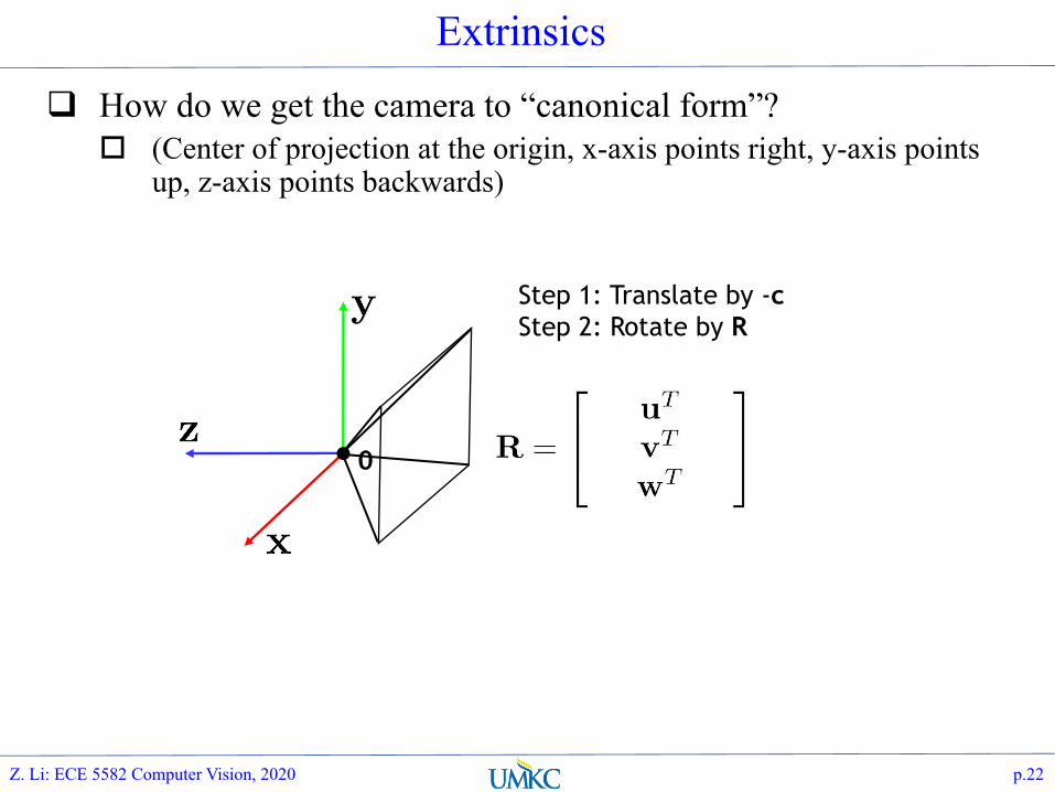
Extrinsics

How do we get the camera to “canonical form”? (Center of projection at the origin, x-axis points right, y-axis points

up, z-axis points backwards)

0

Step 1: Translate by -cStep 2: Rotate by R


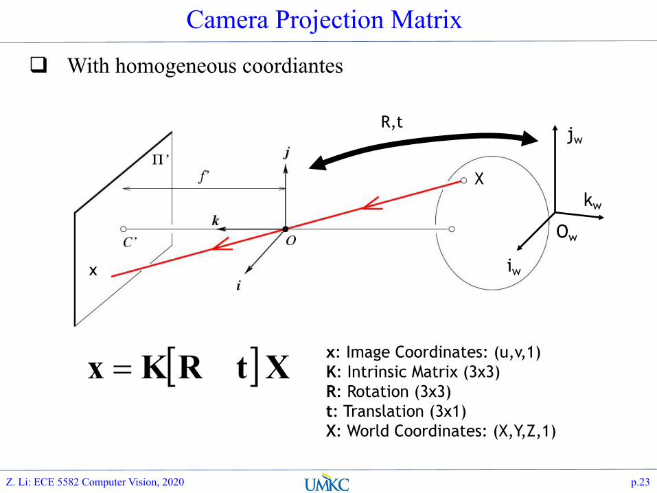
Camera Projection Matrix

With homogeneous coordiantes


[ ]XtRKx = x: Image Coordinates: (u,v,1)K: Intrinsic Matrix (3x3)R: Rotation (3x3) t: Translation (3x1)X: World Coordinates: (X,Y,Z,1)

Ow

iw

kw

jwR,t

X

x

Outline

Recap of Lec 02 Projection Geometry of Image Formation Homography how images of the same 3D scene are related

Summary


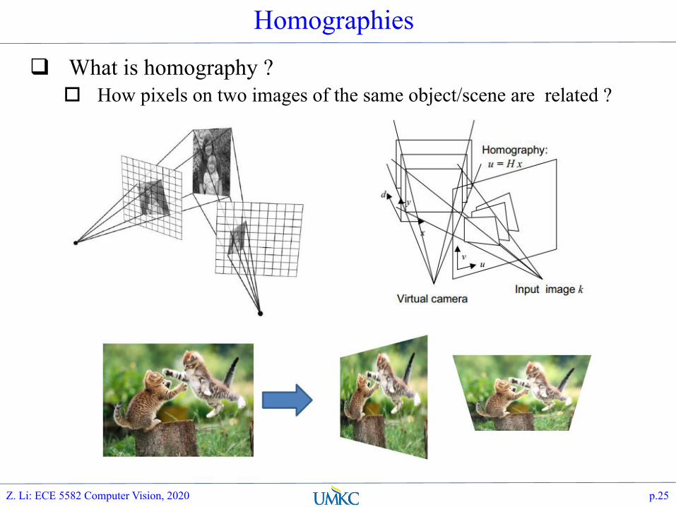
Homographies

What is homography ? How pixels on two images of the same object/scene are related ?


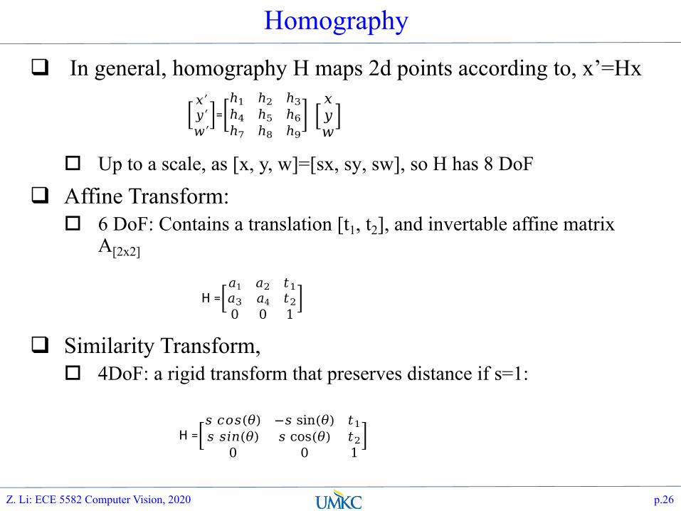
Homography

In general, homography H maps 2d points according to, x’=Hx

Up to a scale, as [x, y, w]=[sx, sy, sw], so H has 8 DoF

Affine Transform: 6 DoF: Contains a translation [t1, t2], and invertable affine matrix

A[2x2]

Similarity Transform, 4DoF: a rigid transform that preserves distance if s=1:


��′�′�′�=�ℎ� ℎ� ℎ�ℎ� ℎ� ℎ�ℎ� ℎ� ℎ�

� ��

H =��1 �� 4 ��0 0 1

�

H =�� X�� −� sin�� X�� cos��

0 0 1�

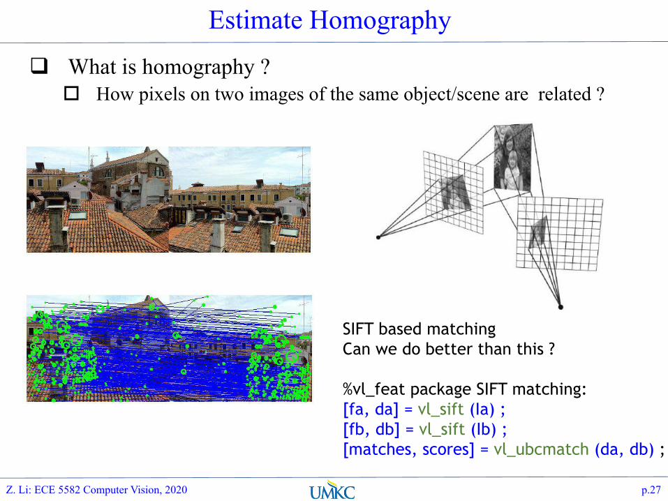
Estimate Homography

What is homography ? How pixels on two images of the same object/scene are related ?


SIFT based matchingCan we do better than this ?

%vl_feat package SIFT matching:[fa, da] = vl_sift (Ia) ;[fb, db] = vl_sift (Ib) ;[matches, scores] = vl_ubcmatch (da, db) ;

Similarity/Affine vs Projective Transform

Similarity vs Affine vs Projective


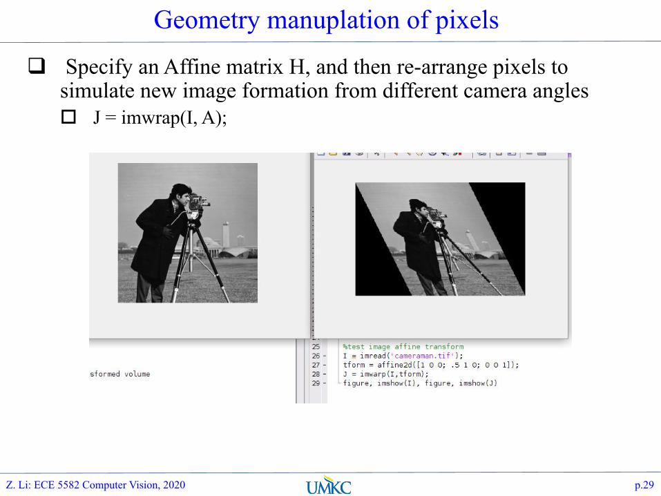
Geometry manuplation of pixels

Specify an Affine matrix H, and then re-arrange pixels to simulate new image formation from different camera angles J = imwrap(I, A);


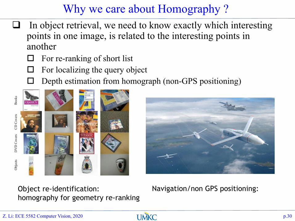
Why we care about Homography ? In object retrieval, we need to know exactly which interesting

points in one image, is related to the interesting points in another For re-ranking of short list For localizing the query object Depth estimation from homograph (non-GPS positioning)


Object re-identification: homography for geometry re-ranking

Navigation/non GPS positioning:

Homography Estimation – DLT Algorithm

To recover H, which has 8 DoF/variables, we just need 4 matching pixel pairs, ideally.

Say if we have 2 points on (u,v) and (x,y) plane matched

s��′�′1� = �

ℎ� ℎ� ℎ�ℎ� ℎ� ℎ�ℎ� ℎ� ℎ�

� ��1�

For each pair, rearranging by dividing first row with the 3rd, and the 2nd row with the 3rd, we have the following,

Do this for 4 points pair: (x1, y1; x’1, y’1),…, (x4, y4; x’4, y’4), we will have 8 equations to solve 8 parameters


�− ℎ� � − ℎ��− ℎ� + �ℎ�� + ℎ��+ ℎ��′ = 0− ℎ�� − ℎ��− ℎ� + �ℎ�� + ℎ� � + ℎ�� = 0

Homography Estimation – DLT Algorithm

In matrix form, we have, Ah = 0 If we have more than 4, then the system is over-determined, we

will find a solution by least squares, computationally via SVD

Pseudo Inverse: SVD: Pseudo inverse (minimizing least square error)


� = �X��

�+ = �X+��

SVD revisited

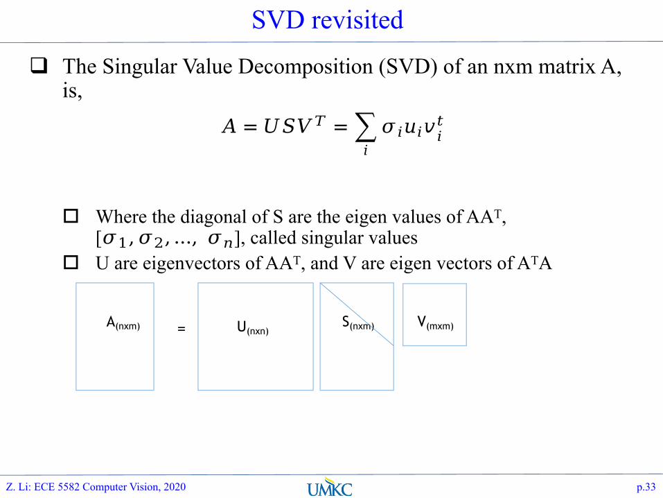
The Singular Value Decomposition (SVD) of an nxm matrix A, is,

Where the diagonal of S are the eigen values of AAT, [��, ��,…, ��], called singular values

U are eigenvectors of AAT, and V are eigen vectors of ATA


� = �X�� =�X��

�

A(nxm) = U(nxn)S(nxm) V(mxm)

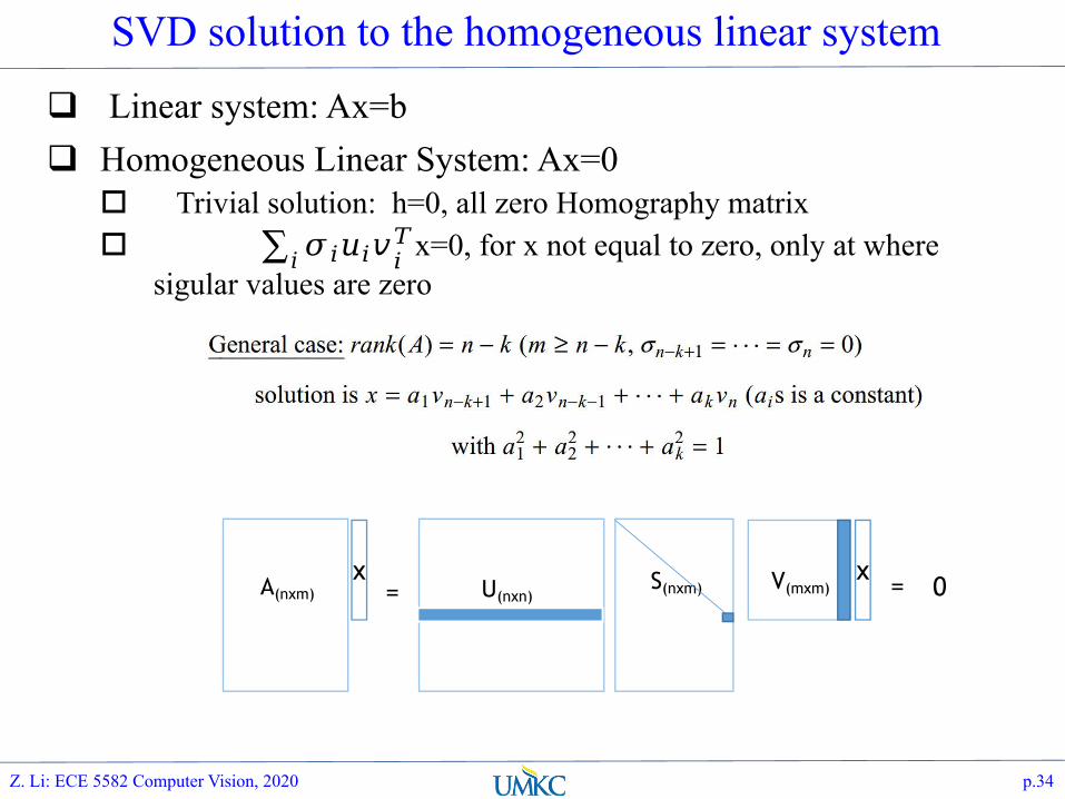
SVD solution to the homogeneous linear system

Linear system: Ax=b Homogeneous Linear System: Ax=0 Trivial solution: h=0, all zero Homography matrix �X��

�x=0, for x not equal to zero, only at where sigular values are zero



xx = 0

Null space of A

Null space of A, x, s.t. Ax=0 Columns of V corresponding to zero singular values are basis

of Null space of A. Hence, any column vector in V corresponds to zero singular

value, are non-trivial solutions to the Ax=0.



xx = 0

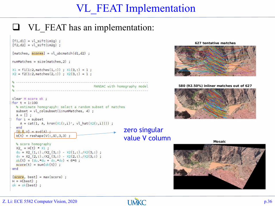
VL_FEAT Implementation

VL_FEAT has an implementation:


zero singularvalue V column

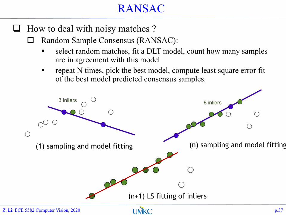
RANSAC

How to deal with noisy matches ? Random Sample Consensus (RANSAC):

select random matches, fit a DLT model, count how many samples are in agreement with this model

repeat N times, pick the best model, compute least square error fit of the best model predicted consensus samples.


(1) sampling and model fitting (n) sampling and model fitting

(n+1) LS fitting of inliers

Application: Panorama Stitching

Create mosaic from multiple images


Summary

Image Formation Pixels not only carry color information, but also carry geometry info Given 3D scene, a camera model, pixels locations on the image

plane is uniquely determined The reverse problem is not as easy (but deep learning is making

good progress on single view depth estimation) Homography: how pixels are related - implications in image

retrieval


Documents

ECE 5582 Computer Vision · Perspective Projection Examples Perspective projection is a simplification of real world image formation Lens characteristics are not considered Perspective