Embed Size (px)
Citation preview

ECE 546 – Jose Schutt-Aine 1
ECE 546 Lecture 02
Review of ElectromagneticsSpring 2014
Jose E. Schutt-AineElectrical & Computer Engineering
University of [email protected]
ECE 546 – Jose Schutt-Aine 2
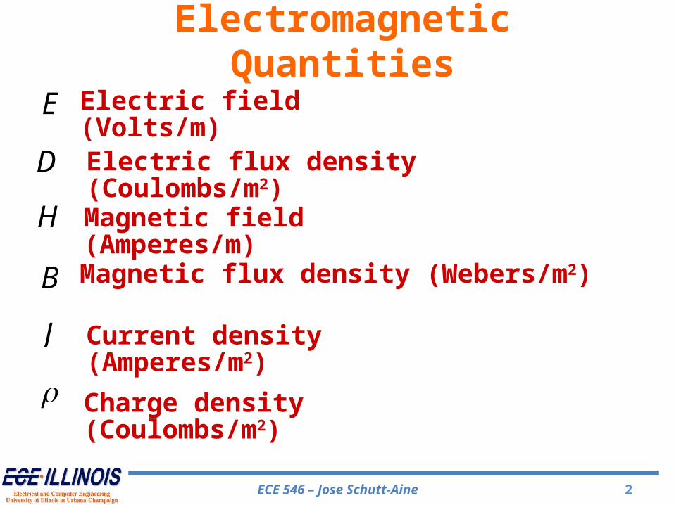
Electromagnetic Quantities
E
HD
B
Electric field (Volts/m)
Magnetic field (Amperes/m)
Electric flux density (Coulombs/m2)
Magnetic flux density (Webers/m2)
J
Current density (Amperes/m2)
Charge density (Coulombs/m2)
ECE 546 – Jose Schutt-Aine 3
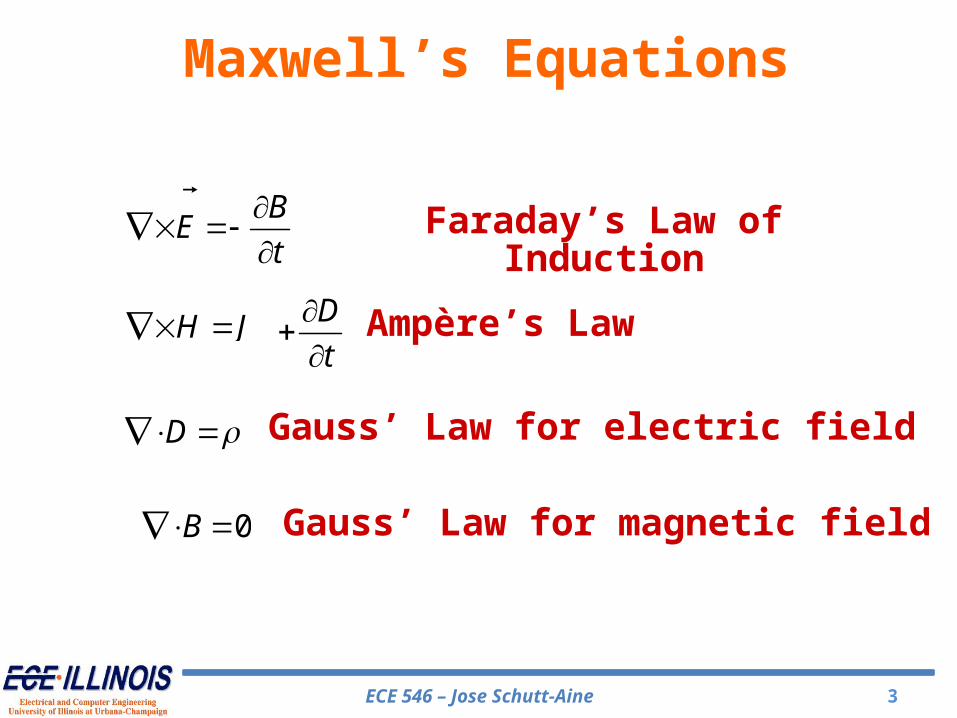
Faraday’s Law of Induction
Ampère’s Law
Gauss’ Law for electric field
Gauss’ Law for magnetic field
BE
t
H J D
t
D
0B
Maxwell’s Equations
ECE 546 – Jose Schutt-Aine 4
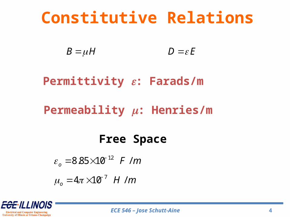
B H
D E
Constitutive Relations
Permittivity e: Farads/m
Permeability m: Henries/m
Free Space
128.85 10 /o F m
74 10 /o H m
ECE 546 – Jose Schutt-Aine 5
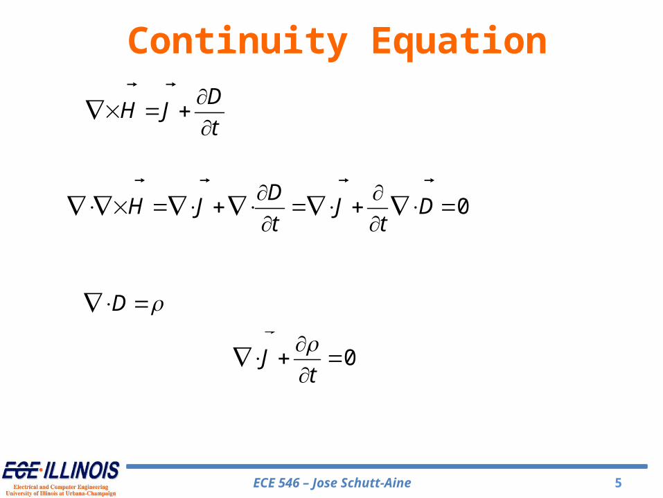
Continuity EquationD
H Jt
0D
H J J Dt t
D
0Jt
ECE 546 – Jose Schutt-Aine 6
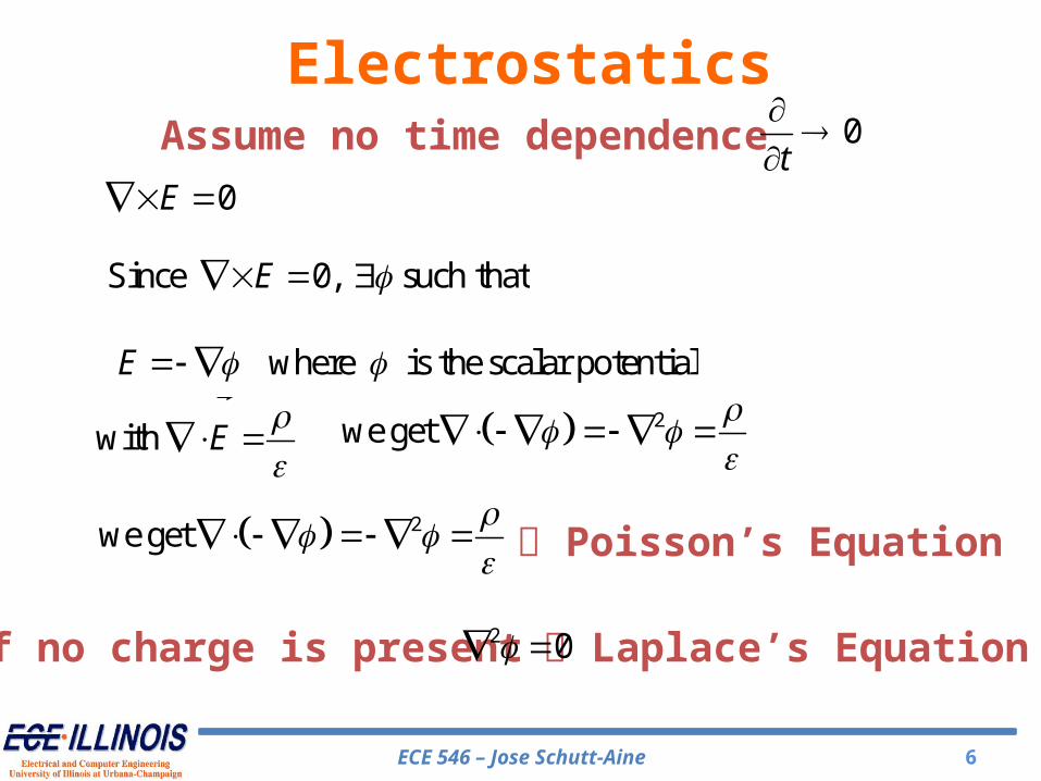
0E
with E
ElectrostaticsAssume no time dependence 0
t
Since 0, such thatE
where is the scalar potentialE
2we get
Poisson’s Equation 2we get
2 0 Laplace’s Equationif no charge is present
ECE 546 – Jose Schutt-Aine 7
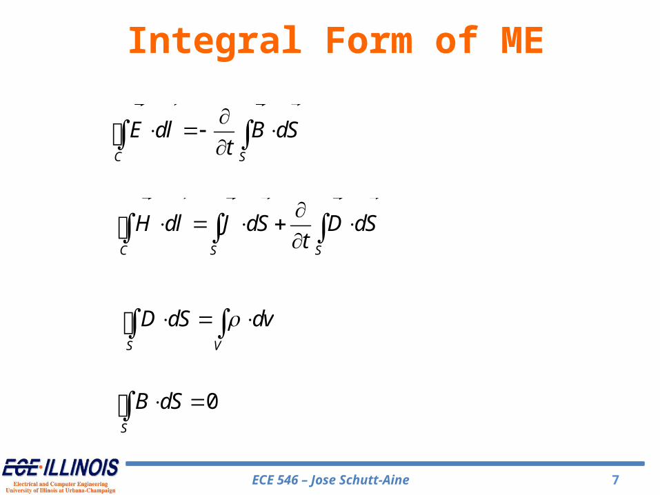
Integral Form of ME
C S
E dl B dSt
C S S
H dl J dS D dSt
S V
D dS dv
0S
B dS
ECE 546 – Jose Schutt-Aine 8
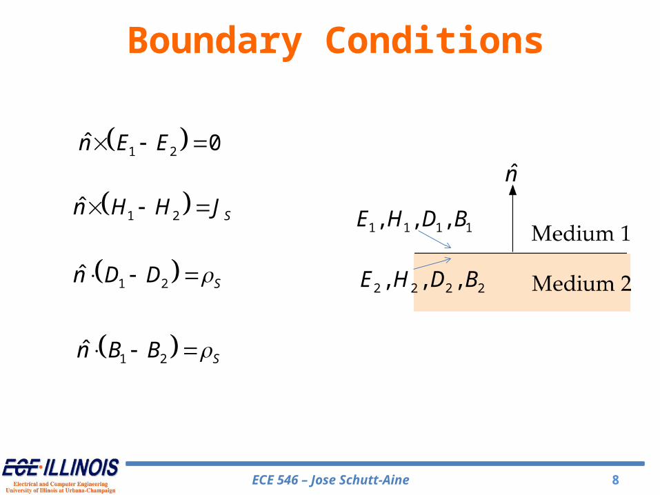
Boundary Conditions
1 2ˆ 0n E E
1 2ˆ Sn H H J
1 2ˆ Sn D D
1 2ˆ Sn B B
n̂
1 1 1 1, , ,E H D B
2 2 2 2, , ,E H D B
ECE 546 – Jose Schutt-Aine 9
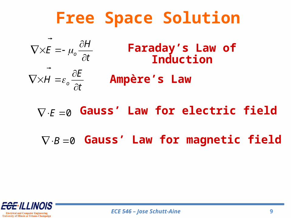
Faraday’s Law of Induction
Ampère’s Law
Gauss’ Law for electric field
Gauss’ Law for magnetic field
o
HE
t
o
EH
t
0E
0B
Free Space Solution

ECE 546 – Jose Schutt-Aine 10
oE Ht
2o o
EE E
t t
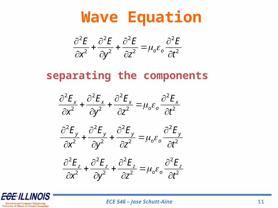
Wave Equation
22
2o o
EE
t
Wave Equation
can show that2
22o o
HH
t
ECE 546 – Jose Schutt-Aine 11
Wave Equation2 2 2 2
2 2 2 2o o
E E E E
x y z t
separating the components
2 2 2 2
2 2 2 2x x x x
o o
E E E E
x y z t
2 2 2 2
2 2 2 2
y y y yo o
E E E E
x y z t
2 2 2 2
2 2 2 2z z z z
o o
E E E E
x y z t
ECE 546 – Jose Schutt-Aine 12
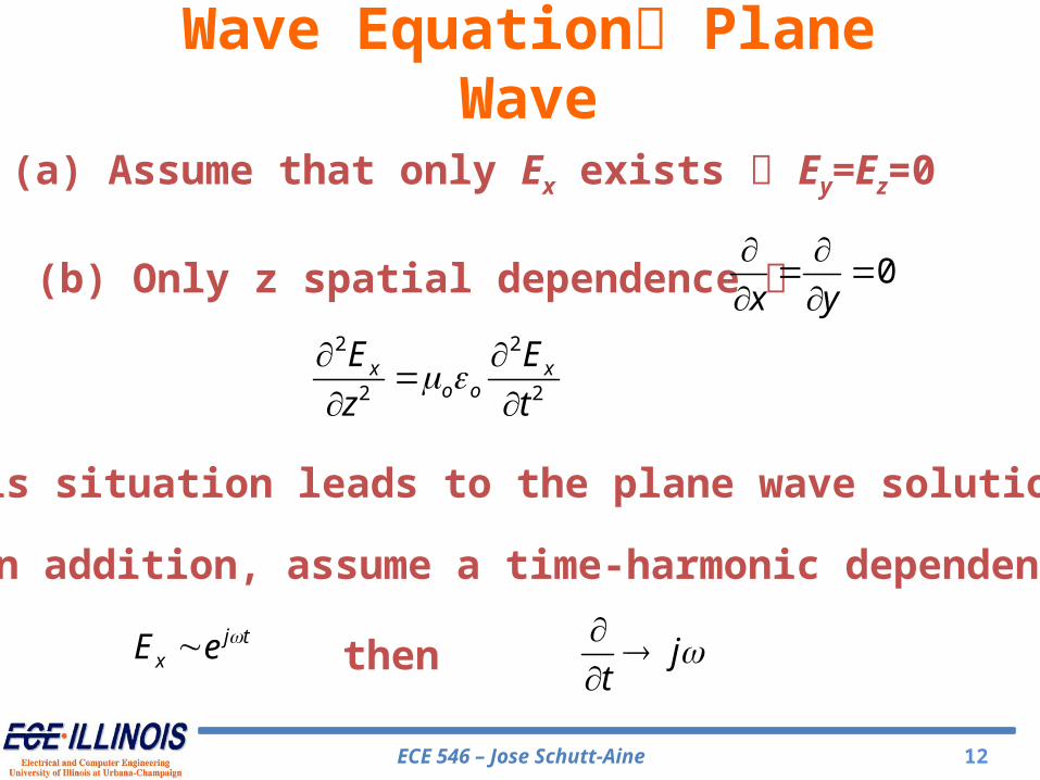
Wave Equation Plane Wave
0x y
(a) Assume that only Ex exists Ey=Ez=0
2 2
2 2x x
o o
E E
z t
(b) Only z spatial dependence
This situation leads to the plane wave solution
In addition, assume a time-harmonic dependence
j txE e then j
t
ECE 546 – Jose Schutt-Aine 13
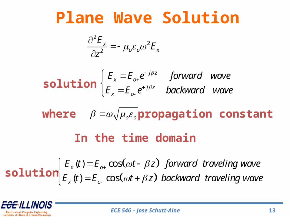
Plane Wave Solution
j zx o
j zx o
E E e forward wave
E E e backward wave
solution
where
In the time domain
22
2x
o o x
EE
z
o o propagation constant
( ) cos
( ) cosx o
x o
E t E t z forward traveling wave
E t E t z backward traveling wave
solution
ECE 546 – Jose Schutt-Aine 14
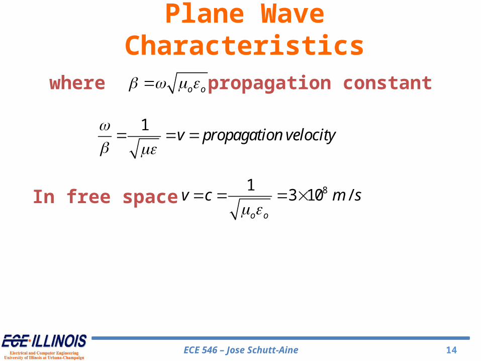
Plane Wave Characteristics
where
In free space
o o propagation constant
1v propagation velocity
813 10 /
o o
v c m s
ECE 546 – Jose Schutt-Aine 15
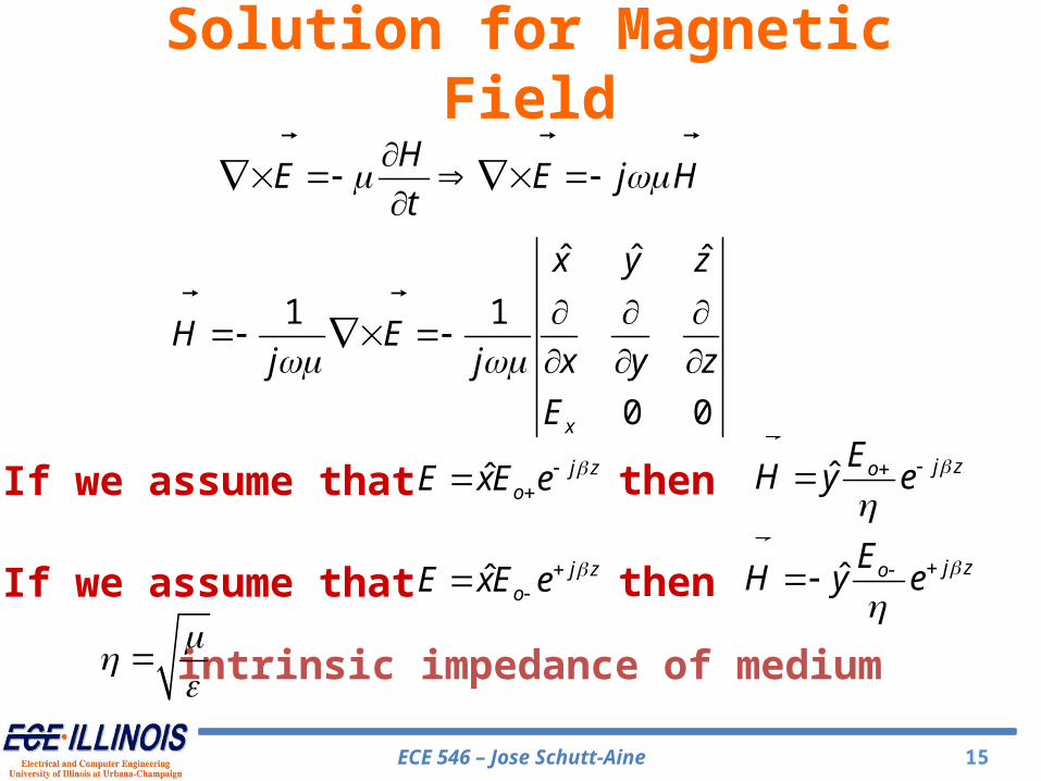
HE E j H
t
Solution for Magnetic Field
ˆ j zoE xE e
If we assume that
ˆ ˆ ˆ
1 1
0 0x
x y z
H Ej j x y z
E
then ˆ j zoEH y e
ˆ j zoE xE e
If we assume that then ˆ j zoE
H y e
intrinsic impedance of medium

ECE 546 – Jose Schutt-Aine 16
( )P t E t H t
Time-Average Poynting Vector
We can show that
Poynting vector W/m2
time-average Poynting vector W/m2
0 0
1 1( )
T TP P t dt E t H t dt
T T
*1Re
2P E H
where and are the phasors of ( ) and ( ) respectivelyE H E t H t
ECE 546 – Jose Schutt-Aine 17
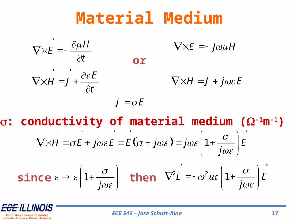
s: conductivity of material medium (W-1m-1)
HE
t
EH J
t
J E
Material Medium
E j H
H J j E
1H E j E E j j Ej
2 2 1E Ej
1
j
or
since then
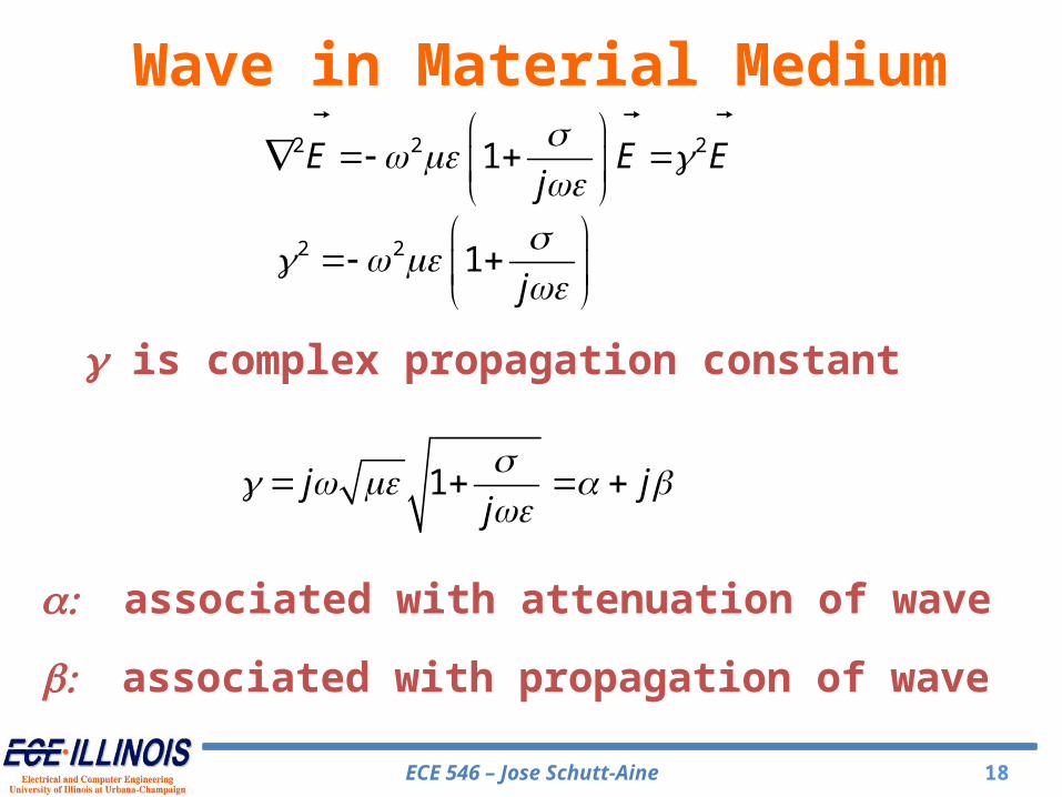
ECE 546 – Jose Schutt-Aine 18
Wave in Material Medium2 2 21E E E
j
g is complex propagation constant
2 2 1j
1j jj
: a associated with attenuation of wave
: b associated with propagation of wave
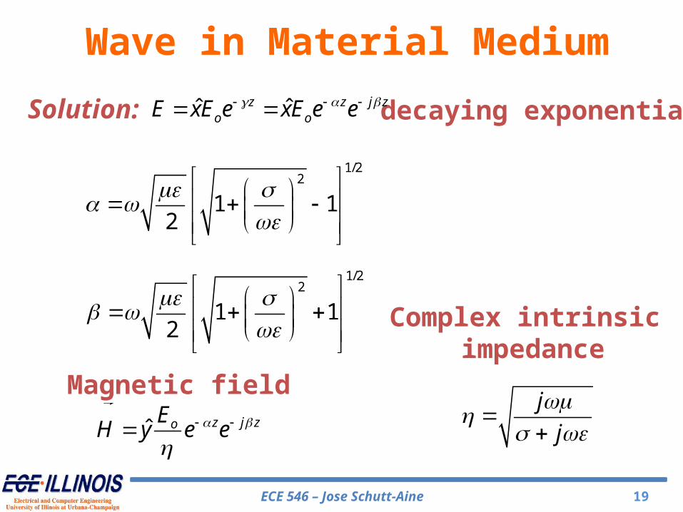
ECE 546 – Jose Schutt-Aine 19
Wave in Material Medium
ˆ ˆz z j zo oE xE e xE e e
1/22
1 12
decaying exponentialSolution:
1/22
1 12
ˆ z j zoEH y e e
j
j
Magnetic field
Complex intrinsic impedance
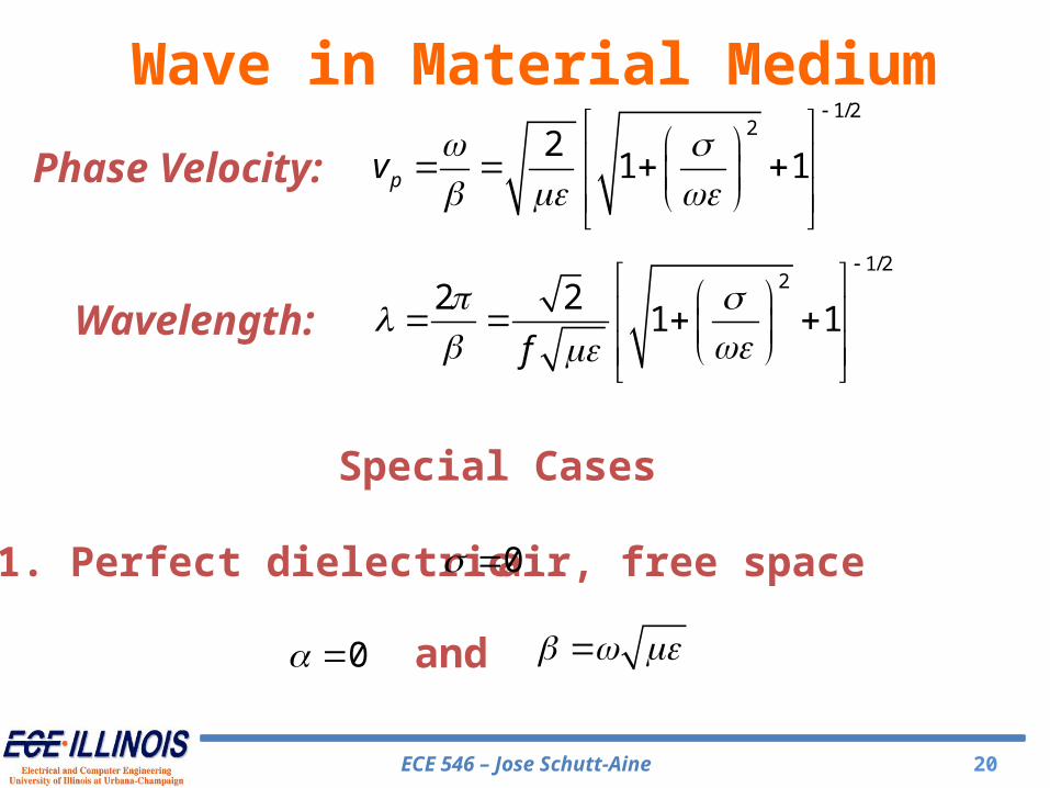
ECE 546 – Jose Schutt-Aine 20
Wave in Material Medium1/2
22
1 1pv
Phase Velocity:
0
0
1. Perfect dielectric
Special Cases
Wavelength:
1/22
2 21 1
f
air, free space
and
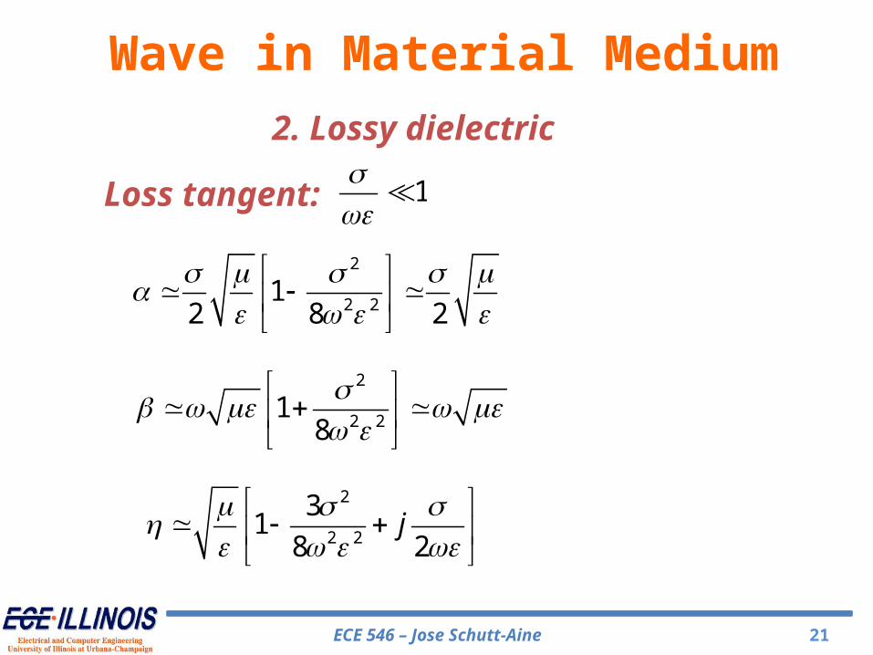
ECE 546 – Jose Schutt-Aine 21
Wave in Material Medium2. Lossy dielectric
Loss tangent: 1
2
2 2
31
8 2j
2
2 21
8
2
2 21
2 8 2

ECE 546 – Jose Schutt-Aine 22
Wave in Material Medium
3. Good conductors
Loss tangent: 1
j j j
f f
1j f
jj
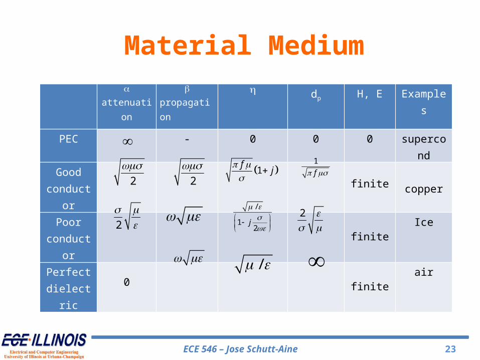
ECE 546 – Jose Schutt-Aine 23
aattenuation
bpropagation
h dp H, E Examples
PEC - 0 0 0 supercond
Good conductor
finite
copper
Poor conductor finite
Ice
Perfectdielectric 0 finite
air
2
2
1f
j
1
f
2
/
12
j
2
/
Material Medium
ECE 546 – Jose Schutt-Aine 24
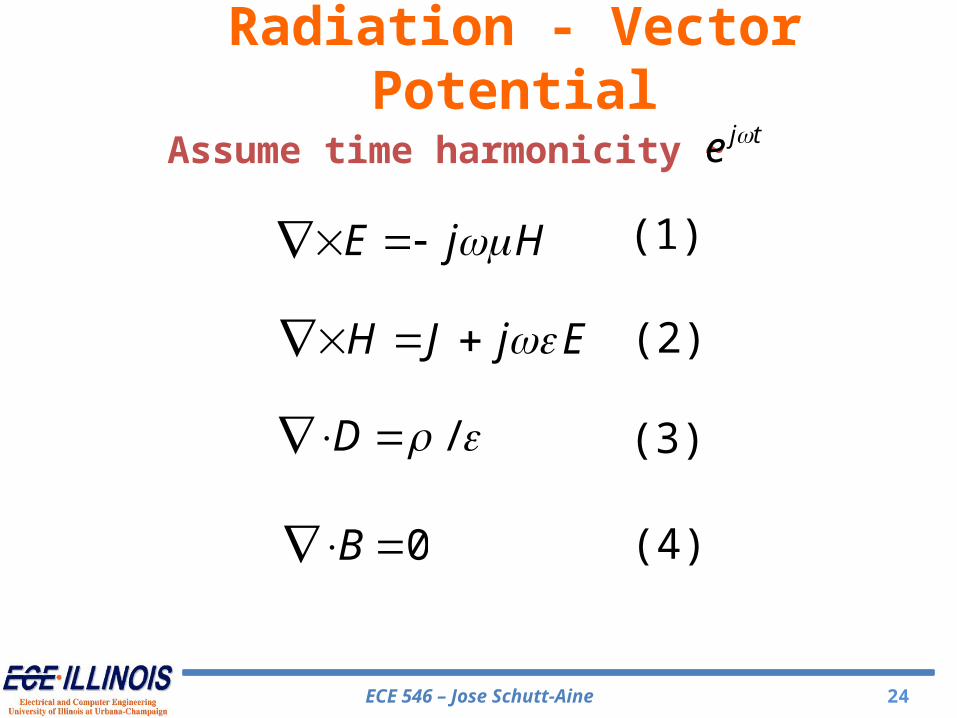
Radiation - Vector Potential
E j H
H J j E
/D
0B
(1)
(2)
(3)
(4)
Assume time harmonicity ~ j te
ECE 546 – Jose Schutt-Aine 25
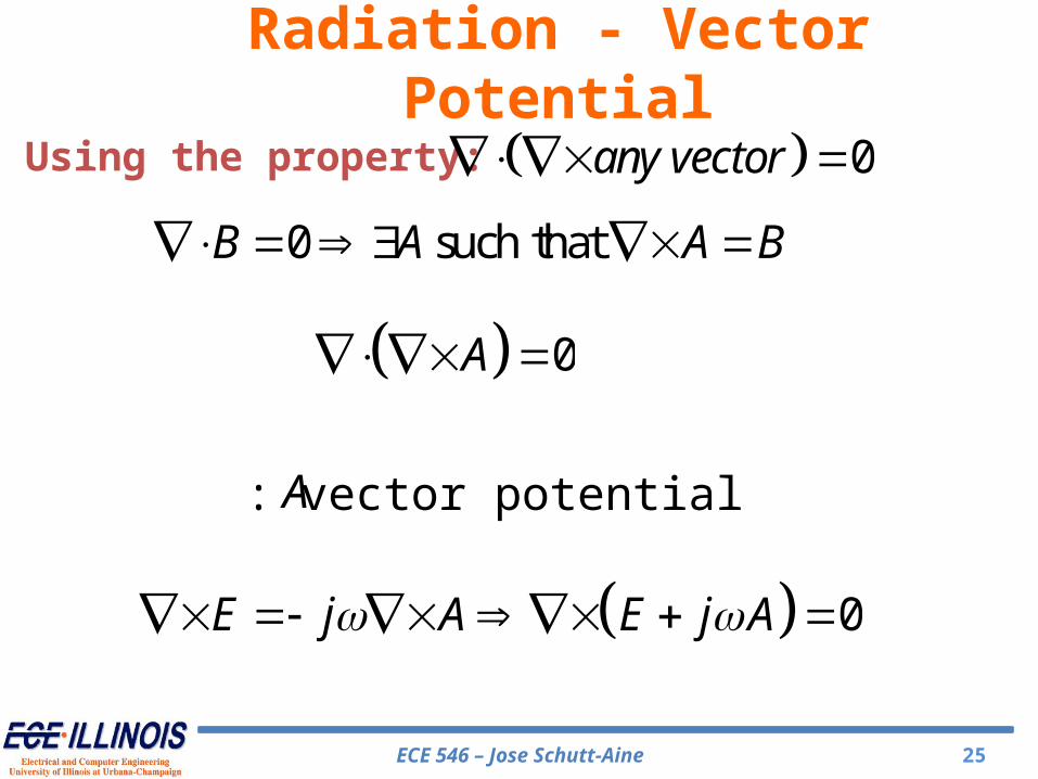
Radiation - Vector Potential
0 such thatB A A B
A
: vector potential
0A
0E j A E j A
Using the property: 0any vector
ECE 546 – Jose Schutt-Aine 2626
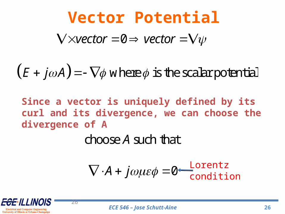
0vector vector
where is the scalar potentialE j A
Since a vector is uniquely defined by its curl and its divergence, we can choose the divergence of A
choose such thatA
0A j Lorentz
condition
Vector Potential
ECE 546 – Jose Schutt-Aine 2727
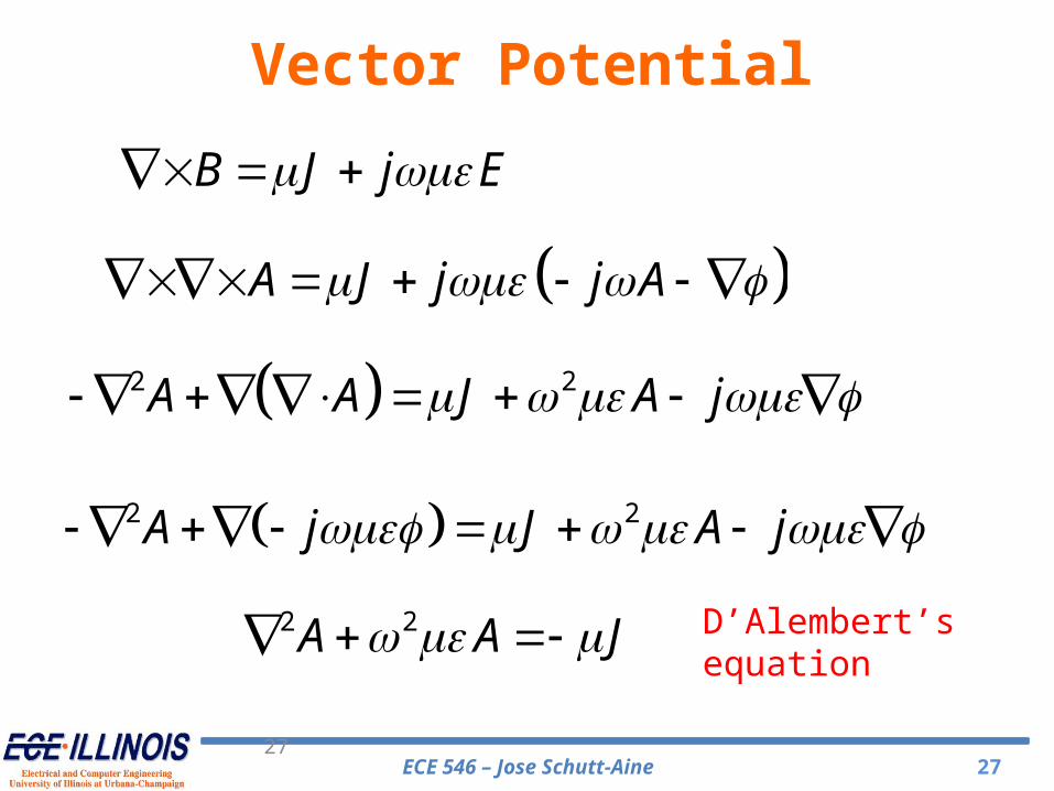
B J j E
A J j j A
2 2A A J A j
2 2A j J A j
2 2A A J
D’Alembert’sequation
Vector Potential
ECE 546 – Jose Schutt-Aine 2828
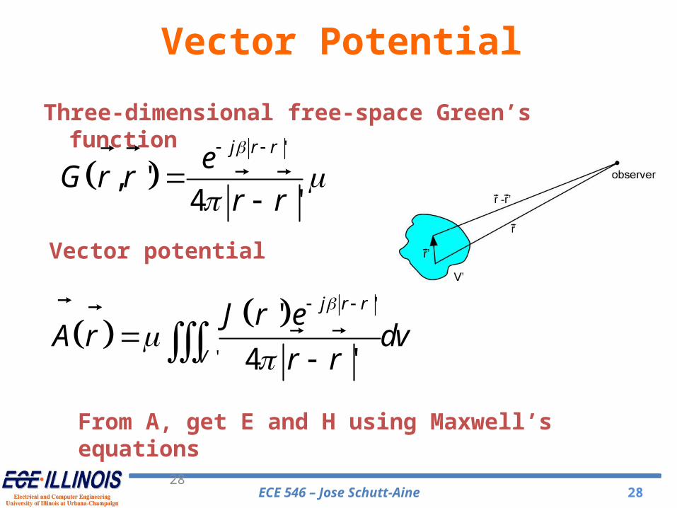
'
, '4 '
j r reG r r
r r
'
'
''
4 '
j r r
V
J r eA r dv
r r
From A, get E and H using Maxwell’s equations
Three-dimensional free-space Green’s function
Vector potential
Vector Potential
ECE 546 – Jose Schutt-Aine 2929
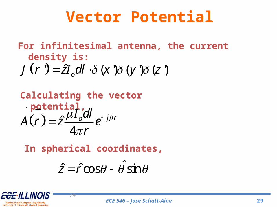
ˆ' ( ') ( ') ( ')oJ r zI dl x y z
For infinitesimal antenna, the current density is:
ˆ4
j roI dlA r z e
r
ˆˆˆ cos sinz r
Calculating the vector potential,
In spherical coordinates,
Vector Potential
ECE 546 – Jose Schutt-Aine 3030
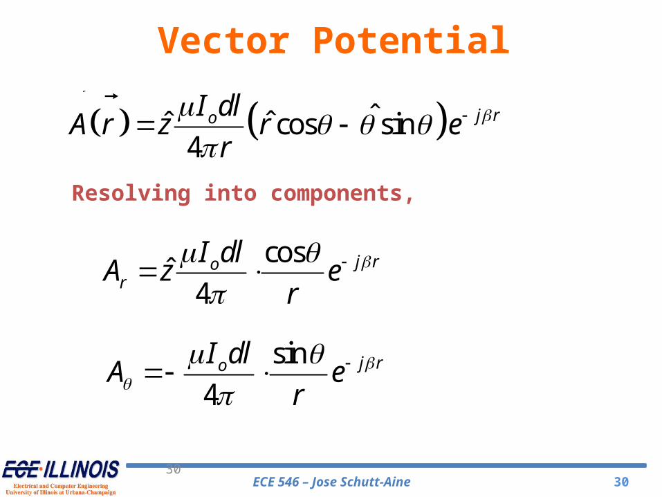
Resolving into components,
ˆˆˆ cos sin4
j roI dlA r z r e
r
cosˆ
4j ro
r
I dlA z e
r
sin
4j roI dl
A er
Vector Potential
ECE 546 – Jose Schutt-Aine 3131
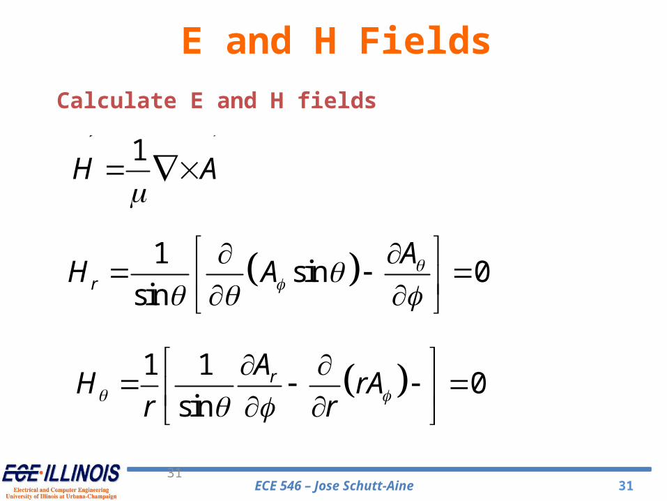
Calculate E and H fields
1H A
1sin 0
sinr
AH A
1 10
sinrAH rA
r r
E and H Fields
ECE 546 – Jose Schutt-Aine 3232
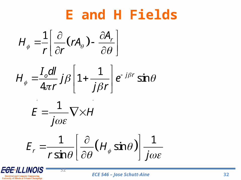
1 rAH rAr r
11 sin
4j roI dl
H j er j r
1E H
j
1 1sin
sinrE Hr j
E and H Fields
ECE 546 – Jose Schutt-Aine 3333
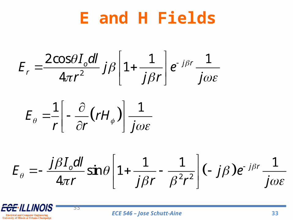
2
2cos 1 11
4j ro
r
I dlE j e
r j r j
1 1E rH
r r j
2 2
1 1 1sin 1
4j roj I dl
E j er j r r j
E and H Fields
ECE 546 – Jose Schutt-Aine 3434
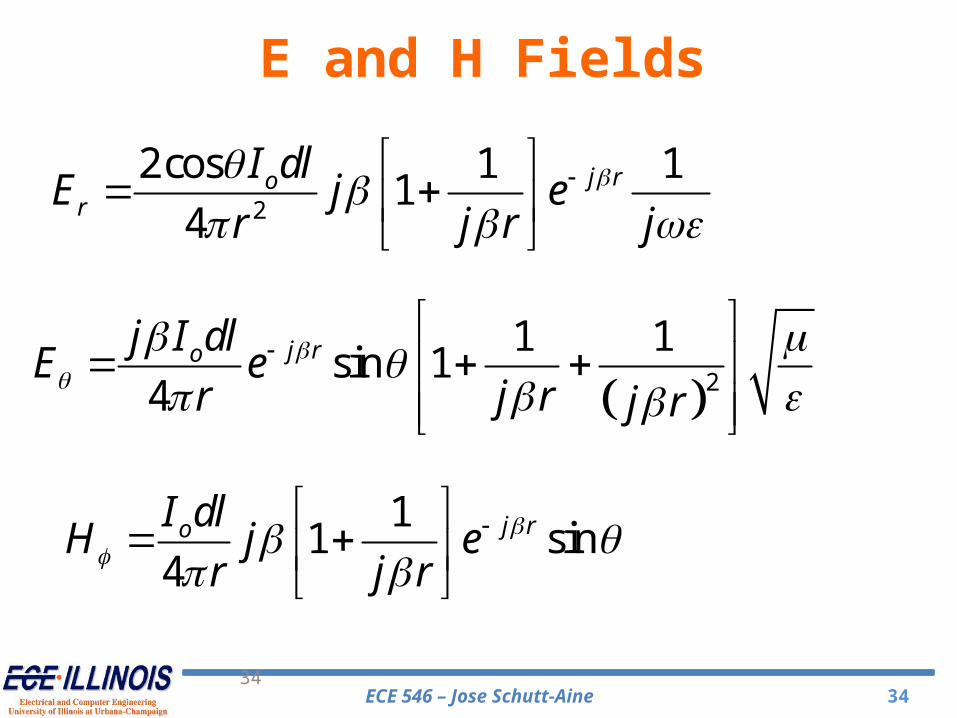
2
1 1sin 1
4j roj I dl
E er j r j r
2
2cos 1 11
4j ro
r
I dlE j e
r j r j
11 sin
4j roI dl
H j er j r
E and H Fields
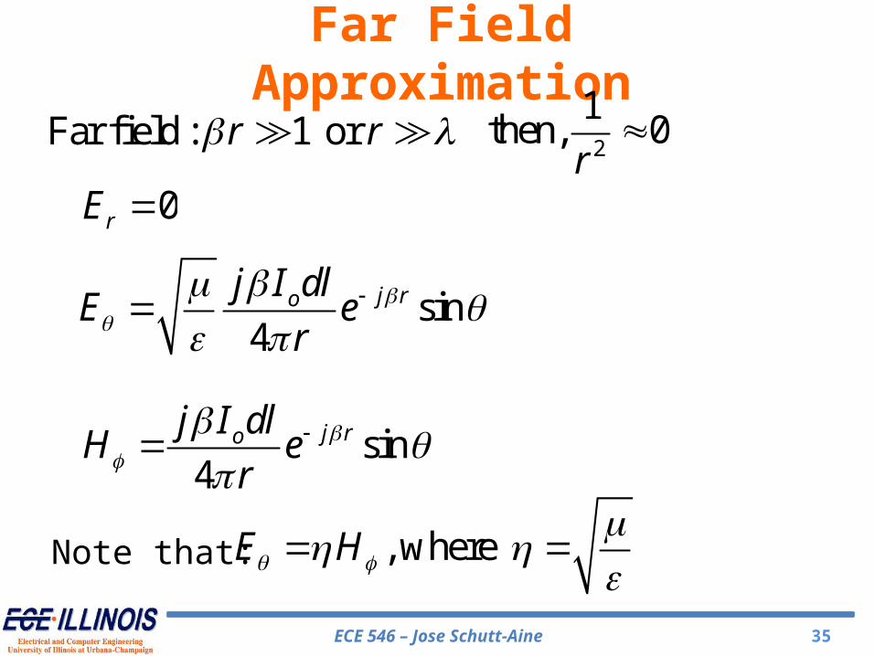
ECE 546 – Jose Schutt-Aine 35
Far field : 1 orr r 2
1then, 0
r
, whereE H
0rE
sin4
j roj I dlH e
r
Note that:
sin4
j roj I dlE e
r
Far Field Approximation
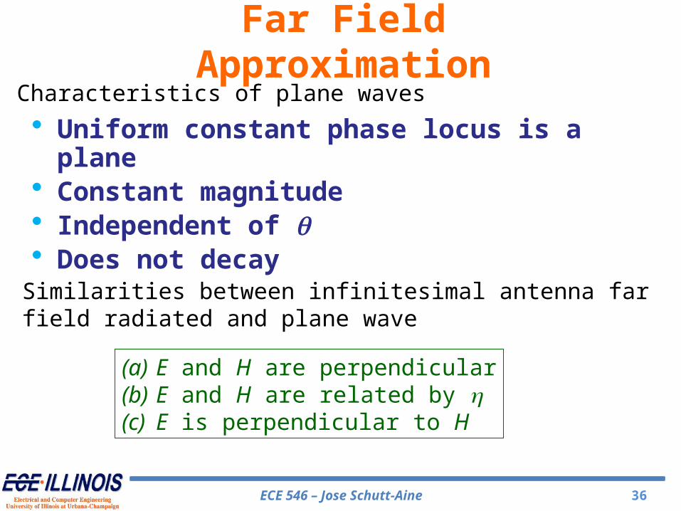
ECE 546 – Jose Schutt-Aine 36
• Uniform constant phase locus is a plane• Constant magnitude• Independent of q• Does not decay
Characteristics of plane waves
Similarities between infinitesimal antenna far field radiated and plane wave
(a) E and H are perpendicular(b) E and H are related by h(c) E is perpendicular to H
Far Field Approximation
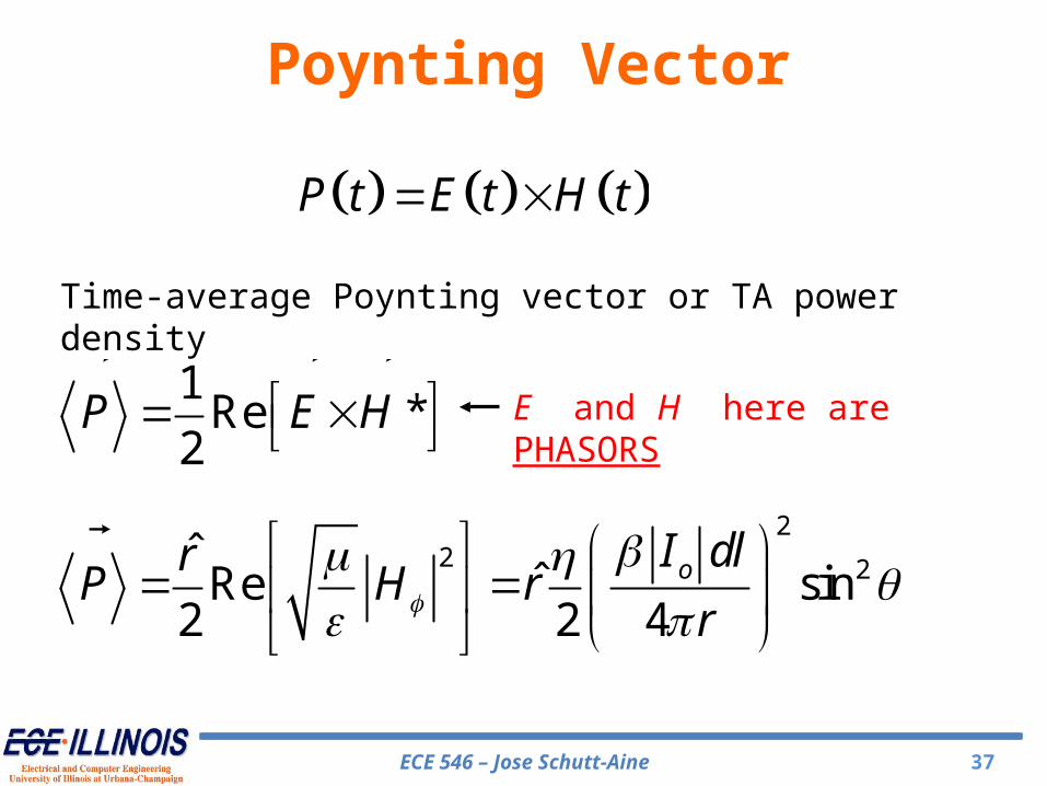
ECE 546 – Jose Schutt-Aine 37
P t E t H t
Time-average Poynting vector or TA power density
1Re *
2P E H
E and H here are PHASORS
22 2ˆ
ˆRe sin2 2 4
oI dlrP H r
r
Poynting Vector
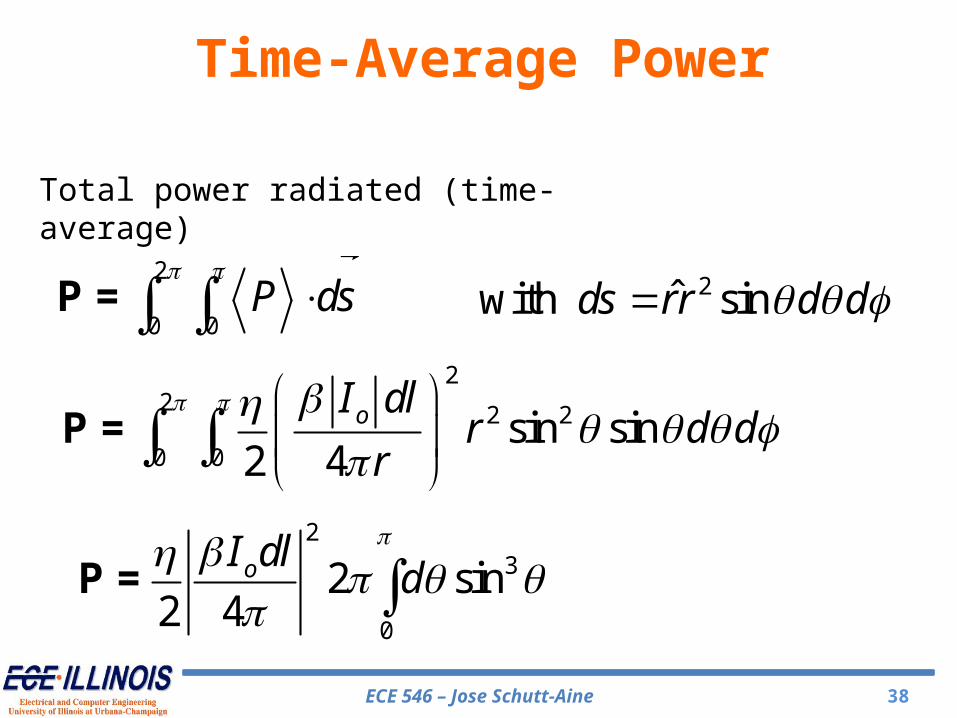
ECE 546 – Jose Schutt-Aine 38
Total power radiated (time-average)
2
0 0P ds
P= 2ˆwith sinds rr d d
22 2 2
0 0sin sin
2 4oI dl
r d dr
P=
23
0
2 sin2 4
oI dld
P=
Time-Average Power
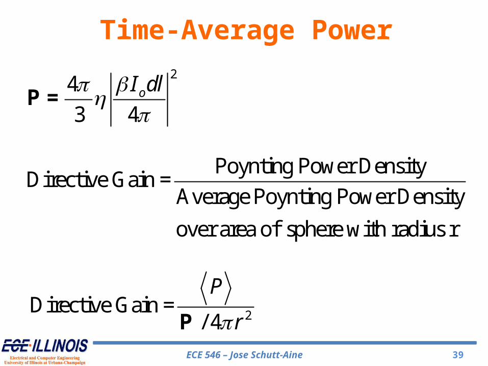
ECE 546 – Jose Schutt-Aine 39
24
3 4oI dl
P=
Poynting Power DensityDirective Gain =
Average Poynting Power Density
over area of sphere with radius r
2Directive Gain =
/ 4
P
r
P
Time-Average Power
ECE 546 – Jose Schutt-Aine 40
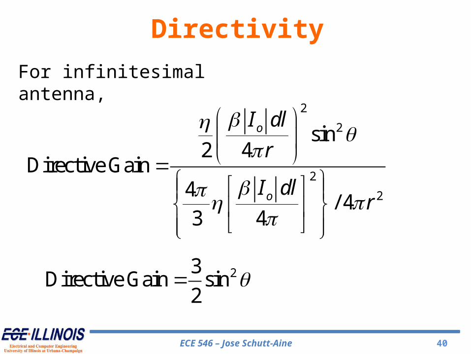
2
2
2
2
sin2 4
Directive Gain4
/ 43 4
o
o
I dl
r
I dlr
For infinitesimal antenna,
23Directive Gain sin
2
Directivity
ECE 546 – Jose Schutt-Aine 41
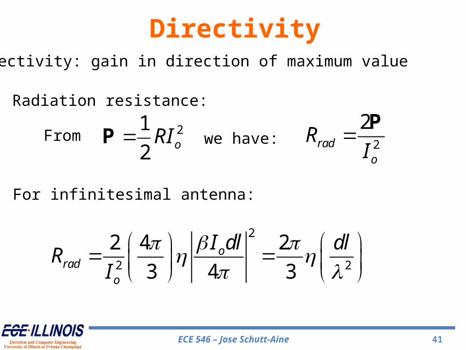
Directivity: gain in direction of maximum value
Radiation resistance:
From 21
2 oRIP we have: 2
2rad
o
RI
P
For infinitesimal antenna:
2
2 2
2 4 2
3 4 3o
rado
I dl dlR
I
Directivity
ECE 546 – Jose Schutt-Aine 42
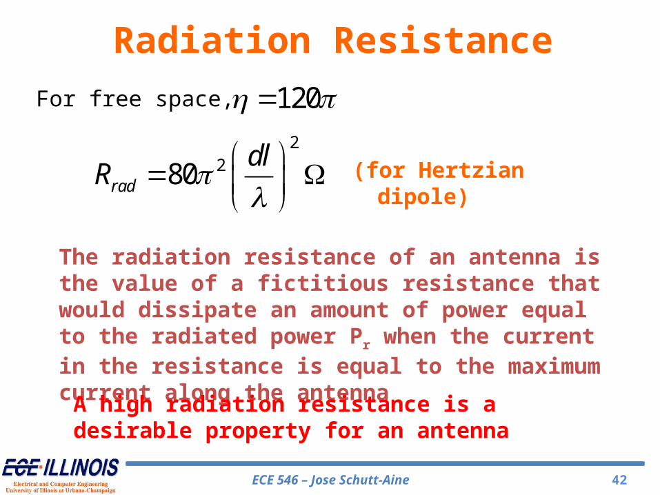
2280rad
dlR
For free space, 120
The radiation resistance of an antenna is the value of a fictitious resistance that would dissipate an amount of power equal to the radiated power Pr when the current in the resistance is equal to the maximum current along the antenna
(for Hertzian dipole)
A high radiation resistance is a desirable property for an antenna
Radiation Resistance