Embed Size (px)
Citation preview

ECE 3355 Electronics
Lecture Notes
Set 3 -- Version 29
Frequency Response and Bode Plots
Dr. Dave Shattuck
Dept. of ECE, Univ. of Houston

Dave ShattuckUniversity of Houston
© University of Houston
Amplifier Frequency Response
• We will cover material from Section 1.6 (pages 31-40) and Appendix E (pages E1-E7) from the 5th Edition of the Sedra and Smith text.
• It may also be useful for you to consult the Nilsson&Riedel Electric Circuits text. The material is from Section 15.6 of the 5th Edition, Section 14.6 of the 6th Edition, or Appendix E of the 7th Edition.

Dave ShattuckUniversity of Houston
© University of Houston
Fourier's Theorem
• Fourier's Theorem says that any physically realizable signal can be represented by, and is equivalent to, a summation of sinusoids of different frequencies, amplitudes and phases.
• Any physically realizable signal translates to any voltage or current, as a function of time, that we can produce or measure.
• Repeat after me: 4-E-A.

Dave ShattuckUniversity of Houston
© University of Houston
Fourier's Theorem
• Fourier's Theorem has profound implications, and represents a significant paradigm shift for electrical engineering.
• We can think of any signal in terms of its frequency components, which are the amplitudes of the sine waves at that frequency. We can find of the response of an amplifier to sinusoids, and predict the response to any signal.
What’s a paradigm?

Dave ShattuckUniversity of Houston
© University of Houston
What are paradigms?
About 20 cents.
Get it? “Pair a dimes?” Okay, so it is not very funny…

Dave ShattuckUniversity of Houston
© University of Houston Fourier's Theorem• Fourier's Theorem has profound
implications, and represents a significant paradigm shift for electrical engineering.
• We can think of any signal in terms of its frequency components, which are the amplitudes of the sine waves at that frequency. We can find of the response of an amplifier to sinusoids, and predict the response to any signal.
What’s a paradigm? A paradigm is a way of thinking about something. A paradigm shift is a change in a way of thinking about something.

Dave ShattuckUniversity of Houston
© University of Houston
Fourier's Theorem
• Fourier's Theorem has profound implications, and represents a significant paradigm shift for electrical engineering.
• We can think of any signal in terms of its frequency components, which are the amplitudes of the sine waves at that frequency. We can find of the response of an amplifier to sinusoids, and predict the response to any signal.
• All of this is made more important by the power of phasor analysis, which makes the analysis of sinusoids relatively easy and quick.
Dave ShattuckUniversity of Houston
© University of Houston
Frequency Response Notation
• To agree with the text, we will use the notation of uppercase variables with lowercase subscripts for phasors. I will not use bold face for the variables when I am writing by hand, but will use it for the text in these notes, to agree with the textbook.
• The phasor of va will be Va.
Dave ShattuckUniversity of Houston
© University of Houston
Frequency Spectrum
• A frequency spectrum of a signal is the plot of the amplitude of each frequency component, plotted vs frequency. We can also plot the phase vs frequency. This is often useful, but in other situations, it can be ignored. It depends.
• We can also plot the response of a circuit to signals versus frequency, and this will be our emphasis in this course. Let's define some more terms.

Dave ShattuckUniversity of Houston
© University of Houston
Transfer Function
• The Phoenician says: Transfer Function = the ratio of the output phasor to the input phasor for a circuit. This is also called the frequency response of the circuit.
)(
)()()(
i
oHTV
V
Dave ShattuckUniversity of Houston
© University of Houston
Transfer Function
)(
)()(
i
oHV
V
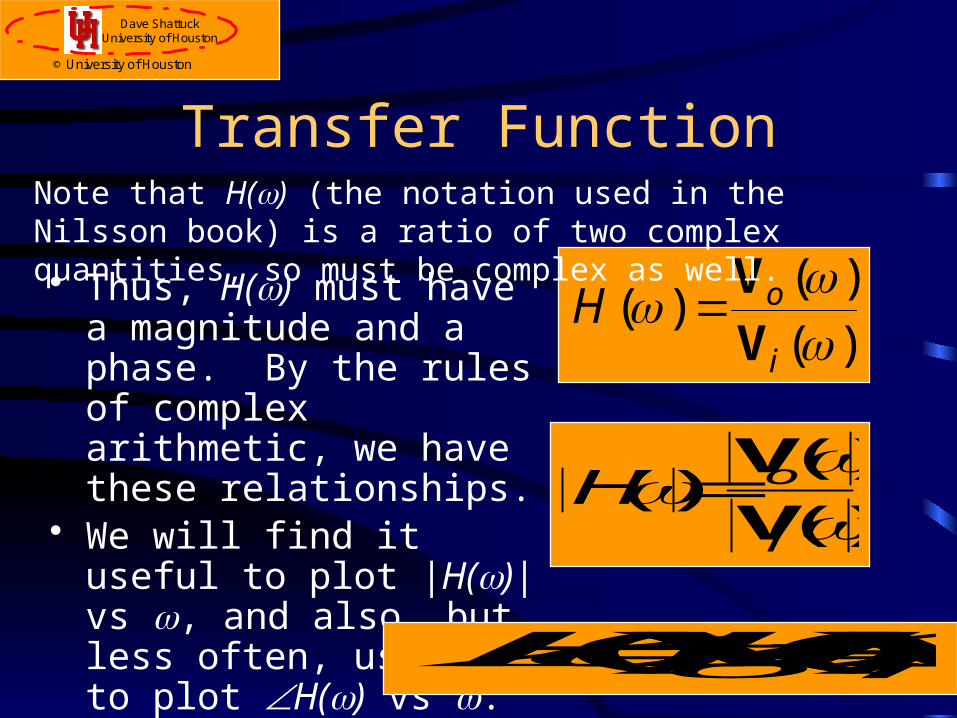
Note that H(w) (the notation used in the Nilsson book) is a ratio of two complex quantities, so must be complex as well.
• Thus, H(w) must have a magnitude and a phase. By the rules of complex arithmetic, we have these relationships.
• We will find it useful to plot |H(w)| vs w, and also, but less often, useful to plot ÐH(w) vs w.
H( ) Vo( )
Vi ( )
H( ) Vo( ) Vi ( )

Dave ShattuckUniversity of Houston
© University of Houston
Transfer Function
• Transfer Function = the ratio of the output phasor to the input phasor for a circuit. This is also called the frequency response of the circuit. Let’s consider a plot of the magnitude of the frequency response as a function of w.
)(
)()(
i
oHV
V

Dave ShattuckUniversity of Houston
© University of Houston
Passband and Bandwidth
• We often call the relatively flat area where the circuit or amplifier is usually used, the passband. The value in this area is called the passband response, or the passband gain. The range of w where this passband is located is called the bandwidth.
)(
)()(
i
oHV
V

Dave ShattuckUniversity of Houston
© University of Houston
• We often call the relatively flat area where the circuit or amplifier is usually used, the passband. The value in this area is called the passband response, or the passband gain. The range of w where this passband is located is called the bandwidth.
• Each of these values can be defined quantitatively. We often plot |H(w)| in dB. Then, we get the 3dB bandwidth, which is the range of w where the response is constant within 3dB of the passband response.
Passband and Bandwidth

Dave ShattuckUniversity of Houston
© University of Houston
• Stated explicitly, we identify a value which represents the gain in the passband. We express this gain in dB, and then subtract 3dB from that value.
• The place where the response intersects this value (passband gain - 3dB) at the top of the passband, we call wH.
• The place where the response intersects this value (passband gain - 3dB) at the bottom of the passband, we call wL.
• The difference between these two values is the 3dB bandwidth, or
3[dB] Bandwidth
BW3dB H L

Dave ShattuckUniversity of Houston
© University of Houston
• We often use circuits with responses that we categorize as a filter. This is where we have a response as a function of frequency with a specific characteristic.
• lowpass filter - passes low frequencies, and attenuates higher frequencies.
• highpass filter - passes high frequencies, and attenuates lower frequencies.
• bandpass filter - attenuates high frequencies, and attenuates lower frequencies.
Filters

Dave ShattuckUniversity of Houston
© University of Houston
But, how do we get these things? Let's do an example problem. I will pick a lowpass RC circuit.a) Find the transfer function, H(w). b) Find the amplitude of the transfer function.c) Find the phase of the transfer function.d) Describe the behavior of each as w®0, and w®¥.
Filter Example

Dave ShattuckUniversity of Houston
© University of Houston
But, how do we get these things? Let's do an example problem. I will pick a lowpass RC circuit.
a) Find the transfer function, H(w).
Solution: Apply the voltage divider rule (in the phasor domain), and we get:
Filter Example
.1
11
1
)( 0
CRjRCj
CjV
VH
s

Dave ShattuckUniversity of Houston
© University of Houston
But, how do we get these things? Let's do an example problem. I will pick a lowpass RC circuit.
b) Find the amplitude of the transfer function.
Filter Example
.
1
1)(
22 CRH

Dave ShattuckUniversity of Houston
© University of Houston
But, how do we get these things? Let's do an example problem. I will pick a lowpass RC circuit.
c) Find the phase of the transfer function.
Filter Example
).arctan()arctan(0)( CRCRH

Dave ShattuckUniversity of Houston
© University of Houston
But, how do we get these things? Let's do an example problem. I will pick a lowpass RC circuit.
d) Describe the behavior of each as w®0, and w®¥.
Actually, it is easier to look at this part by going back to the solution in a). Specifically, for small w, then (1+jwCR) is approximately just 1, and
and for large w, then (1+jwCR) is approximately just jwCR, and
Filter Example
1)( H
.1
)(CRj
H

Dave ShattuckUniversity of Houston
© University of Houston
Note that we have one behavior for the real part of the denominator dominant, and another for the imaginary part dominant.
In other words, we have one behavior forwCR >> 1,
and another forwCR << 1.
The crossover point is where wCR = 1, or where w = 1 / CR.
We call this the breakpoint frequency, for reasons which will become obvious later.
Filter Example
Dave ShattuckUniversity of Houston
© University of Houston
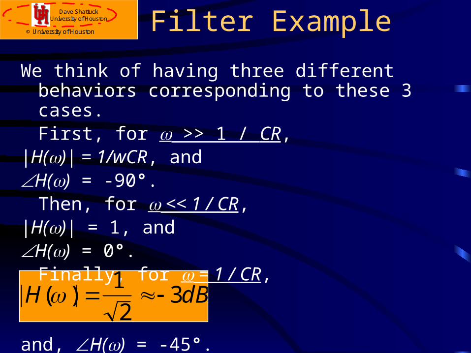
We think of having three different behaviors corresponding to these 3 cases. First, for w >> 1 / CR,
|H(w)| = 1/wCR, and ÐH(w) = -90°.
Then, for w << 1 / CR,|H(w)| = 1, and ÐH(w) = 0°.
Finally, for w = 1 / CR,
and, ÐH(w) = -45°.
Filter Example
H( ) 12
3dB

Dave ShattuckUniversity of Houston
© University of Houston
We now consider Bode Plots. With Bode Plots, we plot the magnitude in dB vs the log of w or f, and plot the phase (on a linear scale) vs the log of w or f.
Bode Plots
Dave ShattuckUniversity of Houston
© University of Houston
We now consider Bode Plots. With Bode Plots, we plot the magnitude in dB vs the log of w or f, and plot the phase (on a linear scale) vs the log of w or f.
Why logarithmic scales? Answer: Because we think logarithmically.
No, really, why do we use logarithmic scales? Answer: Because we think logarithmically. Prove
this using dollar bills.
If this proof is not convincing, I don't think I can prove it to you.
Bode Plots

Dave ShattuckUniversity of Houston
© University of Houston
We now consider Bode Plots. With Bode Plots, we plot the magnitude in dB vs the log of w or f, and plot the phase (on a linear scale) vs the log of w or f.
Now, we can see why Bode plots are so useful. Bode plots tell us everything we need to know about the response of an amplifier, and gives it to us in the most useful possible way, the way that reflects best the values that we have. In the material that follows, we will show a way of plotting them quickly and easily.
Bode Plots

Dave ShattuckUniversity of Houston
© University of Houston
We now consider Bode Plots. With Bode Plots, we plot the magnitude in dB vs the log of w or f, and plot the phase (on a linear scale) vs the log of w or f.
Tells us everything. Most useful form. Easy to plot.
This is nerd heaven. I know
I love Bode Plots. Maybe you will, too. See for yourself.
Bode Plots

Dave ShattuckUniversity of Houston
© University of Houston
Bode Plots are plots of the magnitude in dB vs the log of w or f, and the phase (on a linear scale) vs the log of w or f.
Bode plots have become associated with the idea of the straight line approximations to these same plots. Note again: The straight line approximations are not the most important reason for using logarithmic plots, but they help make them even more useful.
Straight-Line Approximations to Bode Plots

Dave ShattuckUniversity of Houston
© University of Houston
If we restrict ourselves to the case of real valued poles and zeroes, then we can obtain the transfer function as a ratio of the product of terms, as
Transfer Function Form
...
...)(
21
21
pjpjzjzjK
H
For this course, the z's and p's will be real.

Dave ShattuckUniversity of Houston
© University of Houston
These values correspond to frequencies where the dominant part of the term is changing:
· from not frequency dependent
· to frequency dependent.
These are values of frequency where the behavior of that term changes. We will call these values breakpoints.
Breakpoints
...
...)(
21
21
pjpjzjzjK
H

Dave ShattuckUniversity of Houston
© University of Houston
These values correspond to frequencies where the dominant part of the term is changing from not frequency dependent to frequency dependent.
Note that for:
w >> zn, (jw + zn) will increase linearly with w, and thus H(w) will increase linearly with w.
w >> pn, (jw + pn) will increase linearly with w, and thus H(w) will decrease linearly with w.
Behavior with Frequency
...
...)(
21
21
pjpjzjzjK
H

Dave ShattuckUniversity of Houston
© University of Houston
These values correspond to frequencies where the dominant part of the term is changing from not frequency dependent to frequency dependent. We would like to find a way to get these breakpoints quickly. We use a mathematical technique: Let j ®w s. Then, we have
Transferance of Dominance
...
...)(
21
21
pspszszsK
sH

Dave ShattuckUniversity of Houston
© University of Houston
In this situation, the
zn's are zeroes, and
pn's are poles.
Therefore, we can use existing mathematic techniques to find the zeroes and poles, and thus find the breakpoints.
Poles and Zeroes
...
...)(
21
21
pspszszsK
sH
Actually, the zn’s and pn’s are the additive inverses of the zeroes and poles. In this course, the sign does not matter.
Dave ShattuckUniversity of Houston
© University of Houston
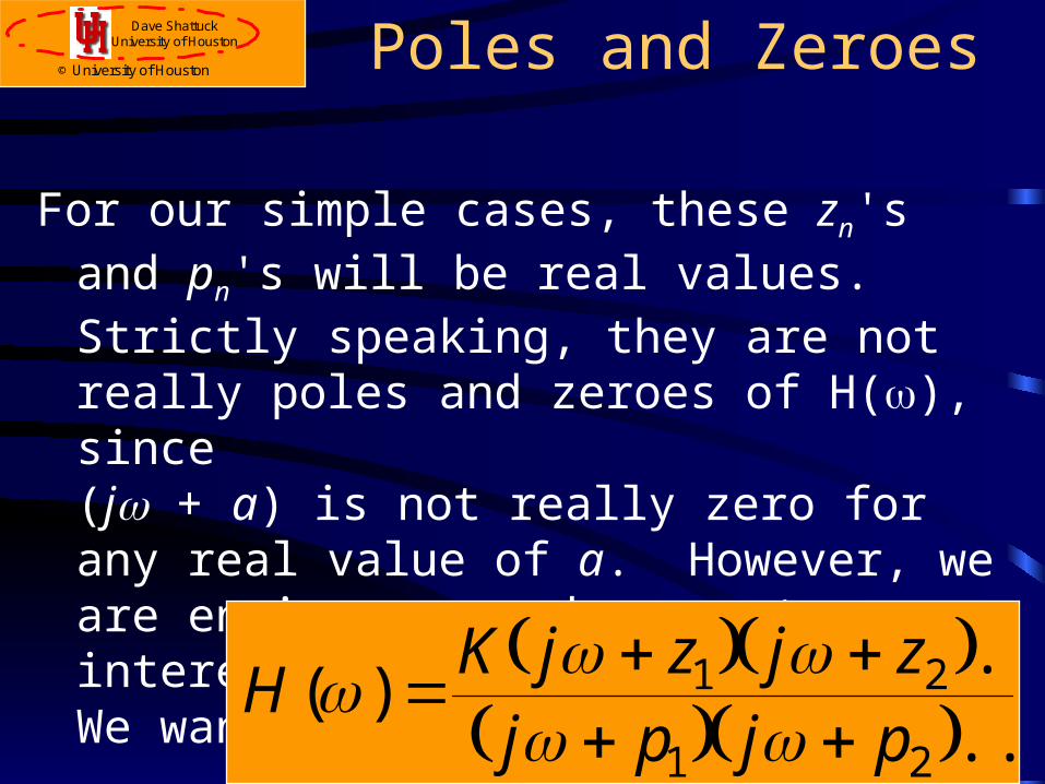
For our simple cases, these zn's and pn's will be real values. Strictly speaking, they are not really poles and zeroes of H(w), since (jw + a) is not really zero for any real value of a. However, we are engineers, and are not interested in speaking strictly. We want useful approximations.
Poles and Zeroes
...
...)(
21
21
pjpjzjzjK
H

Dave ShattuckUniversity of Houston
© University of Houston
In other courses, we will worry about the signs of the poles and zeroes. For the purposes of this course, we will not worry about these signs. We will have plenty to worry about. We will limit the cases we consider to situations where the sign doesn't matter.
Poles and Zeroes
...
...)(
21
21
pjpjzjzjK
H
Worry about signs!

Dave ShattuckUniversity of Houston
© University of Houston
Our approach to plotting Bode plots using the straight line approximations:
1. Obtain the transfer function H(w).
2. Let j ®w s. Find the poles and zeroes of H(s). Take the absolute values of each.
Straight Line Approximation Rules

Dave ShattuckUniversity of Houston
© University of Houston
3. Plot the Magnitude Plot
A. Evaluate |H(w)| at some w. Pick an easy spot.
B. Plot the straight line approximation.
i. At poles, the slope decreases by 20[dB/decade] as you move to the right.
ii. At zeroes, the slope increases by 20[dB/decade] as you move to the right.
Straight Line Approximation Rules

Dave ShattuckUniversity of Houston
© University of Houston
C. (optional) Mark off some corrections to these straight lines, and plot more accurate curves.
i. At poles, label a point 3[dB] below the straight line approximation.
ii. At zeroes, label a point 3[dB] above the straight line approximation.
iii. Draw a smooth curve through these points using the straight lines as asymptotes.
Straight Line Approximation Rules

Dave ShattuckUniversity of Houston
© University of Houston
D. For multiple poles and zeroes, increase the effects proportionately.
i. If you have nz zeroes, the slope increases by nz x 20[dB/dec], and the correction at the breakpoint is nz x 3[dB].
ii. If you have np poles, the slope decreases by np x 20[dB/dec], and the correction at the breakpoint is np x 3[dB].
Straight Line Approximation Rules

Dave ShattuckUniversity of Houston
© University of Houston
4. To Plot the Phase Plot
A. Evaluate ÐH(w) at some w. Pick an easy spot. B. Plot the straight line approximation.
i. At p/10, the slope decreases by 45[°/decade] as you move to the right, for 2 decades only (until 10p).
ii. At z/10, the slope increases by 45[°/decade] as you move to the right, for 2 decades only (until 10z).
Straight Line Approximation Rules

Dave ShattuckUniversity of Houston
© University of Houston
C. (optional) Mark off some corrections to these straight lines, and plot more accurate curves.
i. At p/10, label a point 5.7° below the straight line approximation.
ii. At 10p, label a point 5.7° above the straight line approximation.
iii. At z/10, label a point 5.7° above the straight line approximation.
iv. At 10z, label a point 5.7° below the straight line approximation.
v. Draw a smooth curve through these points using the straight lines as asymptotes.
Straight Line Approximation Rules

Dave ShattuckUniversity of Houston
© University of Houston
D. For multiple poles and zeroes, increase the effects proportionately.
i. If you have nz zeroes, the slope increases by nz x 45[°/dec], and the correction at the breakpoints is nz x 5.7°.
ii. If you have np poles, the slope decreases by np x 45[°/dec], and the correction at the breakpoints is np x 5.7°.
Straight Line Approximation Rules
Dave ShattuckUniversity of Houston
© University of Houston
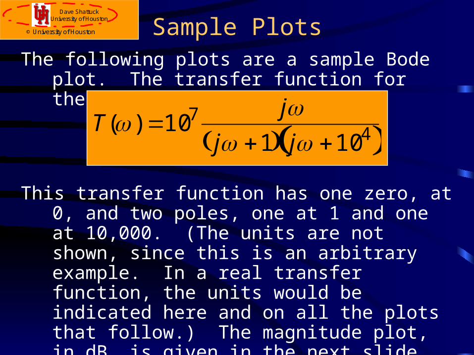
The following plots are a sample Bode plot. The transfer function for these plots is
This transfer function has one zero, at 0, and two poles, one at 1 and one at 10,000. (The units are not shown, since this is an arbitrary example. In a real transfer function, the units would be indicated here and on all the plots that follow.) The magnitude plot, in dB, is given in the next slide. Note that the straight line approximations, also drawn, approach the actual curve assymptotically away from the breakpoints.
Sample Plots
T( ) 107 jj 1 j 104

Dave ShattuckUniversity of Houston
© University of Houston Sample Plots
Magnitude Plot
-10
0
10
20
30
40
50
60
0.001 0.01 0.1 1 10 100 1000 10000 100000 1000000
Frequency (log scale)
Magnitude in dBStraight line approx.

Dave ShattuckUniversity of Houston
© University of Houston
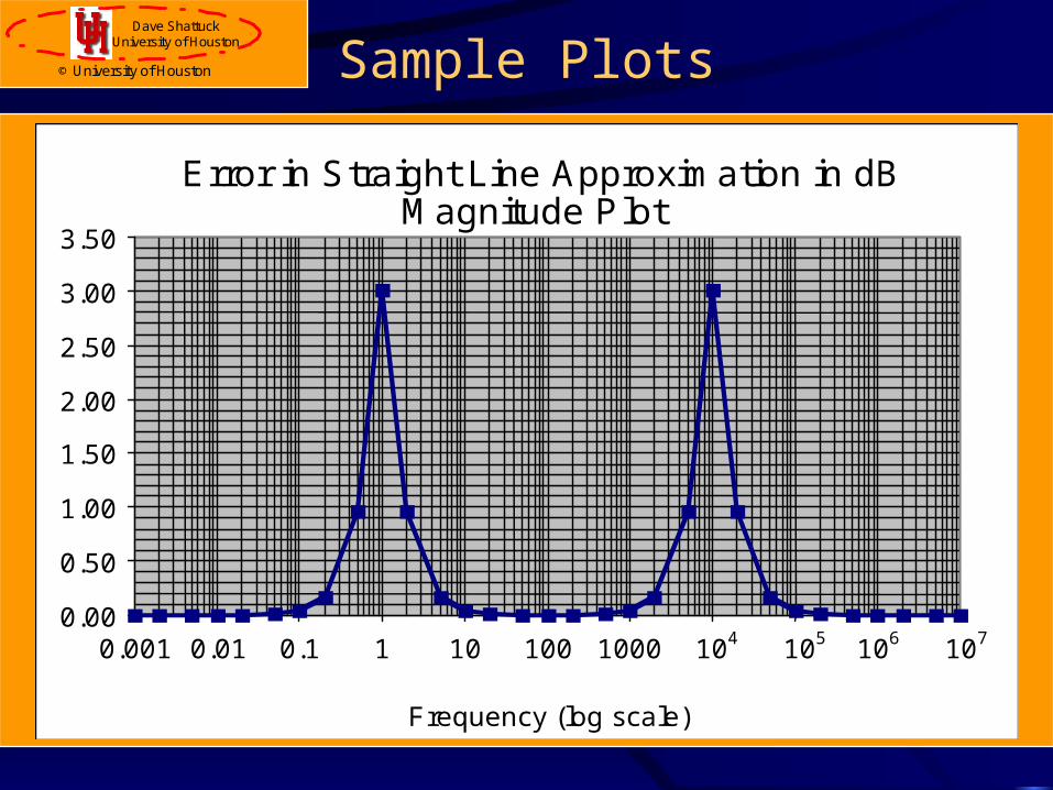
The following plots are a sample Bode plot. The transfer function for these plots is
This transfer function has one zero, at 0, and two poles, one at 1 and one at 10,000. Now, if we plot the error between the actual plot and the straight-line approximation, we get the plot in the following slide.
Sample Plots
T( ) 107 jj 1 j 104
Dave ShattuckUniversity of Houston
© University of Houston Sample Plots
Error in Straight Line Approximation in dB
Magnitude Plot
0.00
0.50
1.00
1.50
2.00
2.50
3.00
3.50
0.001 0.01 0.1 1 10 100 1000 104 105
106 107
Frequency (log scale)

Dave ShattuckUniversity of Houston
© University of Houston
The following plots are a sample Bode plot. The transfer function for these plots is
This transfer function has one zero, at 0, and two poles, one at 1 and one at 10,000. Now, if we plot the phase plot, we get the plot in the following slide.
Sample Plots
T( ) 107 jj 1 j 104

Dave ShattuckUniversity of Houston
© University of Houston Sample Plots
Phase Plot in Degrees
-100
-80
-60
-40
-20
0
20
40
60
80
100
10-2 10-1 100 101 102 103 104 105 106 107
Frequency (log scale)
Phase (in degrees)Straight line approx.

Dave ShattuckUniversity of Houston
© University of Houston
The following plots are a sample Bode plot. The transfer function for these plots is
This transfer function has one zero, at 0, and two poles, one at 1 and one at 10,000. Now, if we plot the error between the actual plot and the straight-line approximation, we get the plot in the following slide.
Sample Plots
T( ) 107 jj 1 j 104

Dave ShattuckUniversity of Houston
© University of Houston Sample Plots
Error in Straight Line Approximation
Phase Plot, in degrees
-6
-4
-2
0
2
4
6
0.01 0.1 1 10 100 1000 104 105
106 107
Frequency (log scale)

Dave ShattuckUniversity of Houston
© University of Houston
The largest errors occur where the straight line approximation has a change in slope. In the magnitude plots, this happens at the locations of the poles and zeroes. In the phase plots, this happens at both a decade above and a decade below the locations of the poles and zeroes.
Errors in Straight-Line Approximations

Dave ShattuckUniversity of Houston
© University of Houston
If you want to look at this data more carefully, it is available in a Microsoft Excel spreadsheet, called Bode_plot_example, which should be available on the network.
Let’s do an example problem.
Work on problem using the overhead projector, showing how semilog graph paper works.
Examples