ECE 3084A Lab 3: Motor Velocity Control

Spring Semester 2015, Section A

Date Lab Performed:

Name/Section of Partner 1:

Name/Section of Partner 2:

Name/Section of Partner 3:

Name/Section of Partner 4:

Goals:

1. Investigate P, PI, and PID speed control for a DC motor.

2. Observe tracking performance for time-varying references.

3. Determine appropriate gains to achieve given best system performance.

4. Understand trade-offs between various system performance parameters like tracking,stability, oscillation, etc.

5. Observe and understand how a real system deviates from an ideal mathematical model.

Preparation:

To perform this lab, you must download and install software. WARNING!!! This pro-cess can take a long time (1 hour or more depending on your download speed).

PC Users

1. You should already have the Elvis suite installed, which has the myDAQ drivers. If itisn’t, or if it isn’t the latest version, you must install it from the following link:

http://www.ni.com/download/ni-elvismx-14.0/4801/en/.

It is over 1.4 GBytes, and takes a really long time (1-2 hours depending on yourconnection speed). Try the rest of the installation before doing this!

2. Install the Runtime Engine (much smaller) from:

http://www.ni.com/download/labview-run-time-engine-2014/4887/en/.

3. Download the zip file “MotorControl-PC.zip” from T-Square (under Lab 3 in Re-sources), and extract the file “Spring15 MotorControlsLab.exe”.

1

Mac Users

1. myDAQ driver only: http://www.ni.com/gate/gb/GB_EVALDAQMXMYDAQ/US

2. Runtime Engine:

http://www.ni.com/download/labview-run-time-engine-2014/4894/en/

3. Download the zip file “MotorControl-MAC.zip” from T-Square (under Lab 3 in Re-sources), and extract the application “Spring15 MotorControlsLab”.

After you have downloaded all software and rebooted your computer, it is critical that youdo the following before you come to class:

1. Plug your myDAQ into your computer.

2. Run the executable (application) “Spring15 MotorControlsLab”.

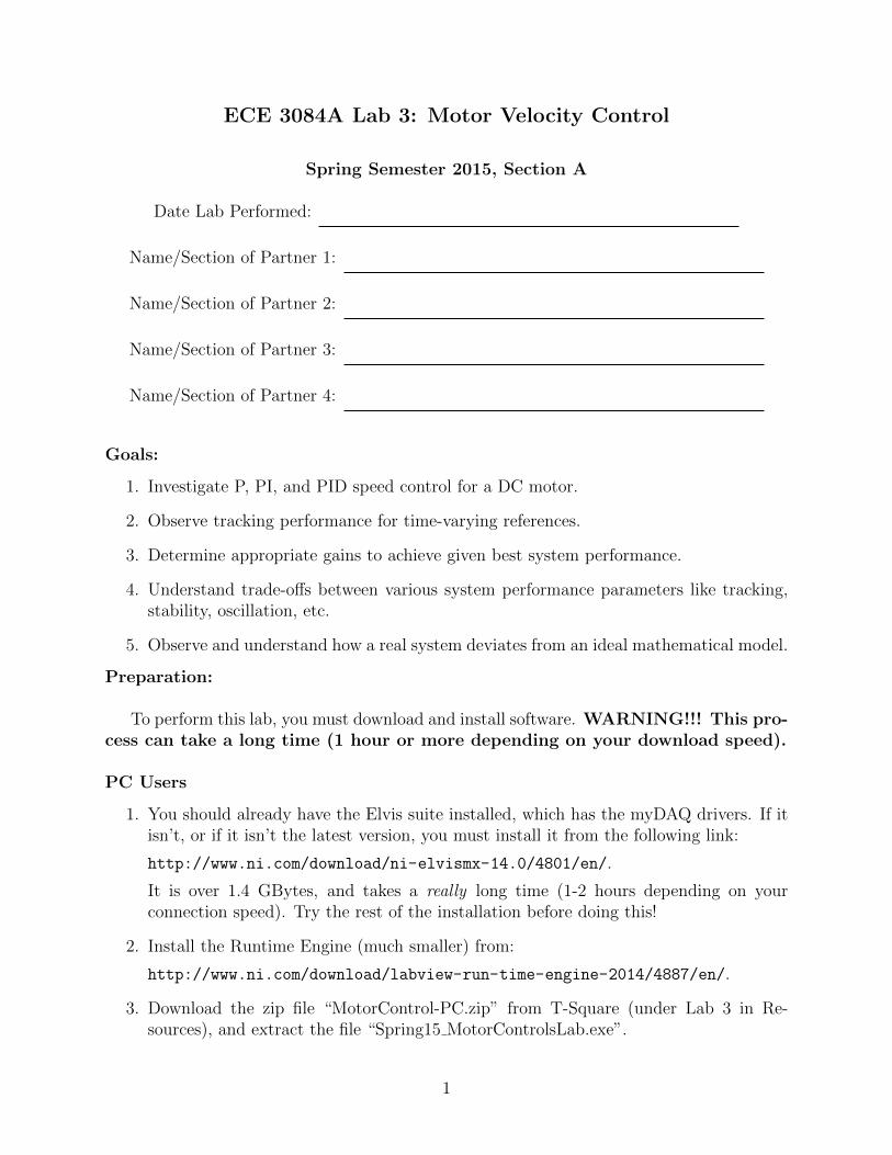
3. Verify that you get the startup screen shown in Figure 1 with no error messages.

4. Verify that you can start it using the small white arrow on top without getting an”Invalid Device” error (use the “Stop” button so you can close the GUI).

Also, carefully read through the entire lab in advance. Bring a printout of the lab toclass with your laptop.

Figure 1: Screenshot of the VI after startup.

2

Background:

This lab demonstrates basic controller design for velocity control of a DC motor. We aregoing to use the LabVIEW myDAQ equipment to control the angular velocity of the motorvia a custom LabVIEW program. The motor is controlled using Pulse Width Modulation(PWM). There are two digital command signals: one is the direction (clockwise or counterclockwise) and the other is the pulse-width modulated signal that controls how much powerthe motor uses. The frequency of this PWM signal is constant, but the larger the duty cycle(percentage of time it is non-zero), the faster the motor turns (a 50% duty cycle means thatit is “on” half of the time). We will make the approximation that the PWM duty cycle isdirectly proportional to the motor speed. This is one reason our open loop controller doesn’twork very well (it is actually non-linear), but using feedback, we can overcome this and othermodeling errors. The position of the motor shaft is measured using an incremental encoder,and the velocity is derived from the position in software.

In the time domain, we have:

1. The dynamics of the motor (the plant) that relate the input x(t) to othe output y(t),usually via a differential equation (Eq. 1).

2. The relationship between the measured output (the angle of the motor) y(t) and thevalue we will use for feedback (angular velocity) y (Eq. 2).

3. An error signal e(t) – how close the actual motor velocity is to the desired velocity r(t)at each time point (Eq. 3).

4. A controller (control function) to generate the input x(t) to the motor based upon theerror e(t) (Eq. 4).

y = f(u, y) (1)

y =dy(t)

dt(2)

e(t) = r(t)− y(t) (3)

x(t) = Kpe(t) +Ki

∫ t

0

e(τ)dτ +Kde(t) (4)

The overall goal of the lab is to choose Kp, Ki, and Kd (the gains) such thatsystem performance specifications are successfully met.

It is useful to view Eqs. 1-4 in the Laplace domain so that we can draw a block diagramto describe the setup. Taking the Laplace transform of each equation, we can define threetransfer functions corresponding to the three blocks in the diagram:

1. Between the error signal and the plant input (the controller), Gc(s).

2. Between the input and the output (the plant), Gp(s).

3

3. Between the output (shaft angular position) and the shaft angular velocity (the tachome-ter), T (s).

Gc(s) Gp(s)x(t)

T (s)

r(t) + e(t) y(t)

−

y(t)

Because the plant output y(t) (the shaft angular position) is inherently noisy, we haveadded a low pass filter to the differentiator to smooth the approximation of the motor’sangular velocity,

T (s) =as

s+ a,

making this block a filtered differentiator. For this setup we have a = 15.Note that

X(s) = Gc(s)E(s)

where

Gc(s) = Kp +Ki

s+Kds.

In discrete time, this controller is implemented in LabView software by the myDAQ as

x[k] = Kpe[k] +Ki

k∑0

e[k]dT +Kd

(e[k]− e[k − 1]

dT

)where k is a discrete representation for time and dT is the width of our time step. HeredT = 0.01 sec.

Experiment:

Figure 2 shows the overall setup of the myDAQ, the printed circuit board (PCB) withattached motor, and the battery pack. Figure 3 shows where the terminals where the batterypack is connected. PC users can verify that your computer is seeing the myDAQ by startingthe NI ELVIS Instrument launcher and opening the scope. You should see static.

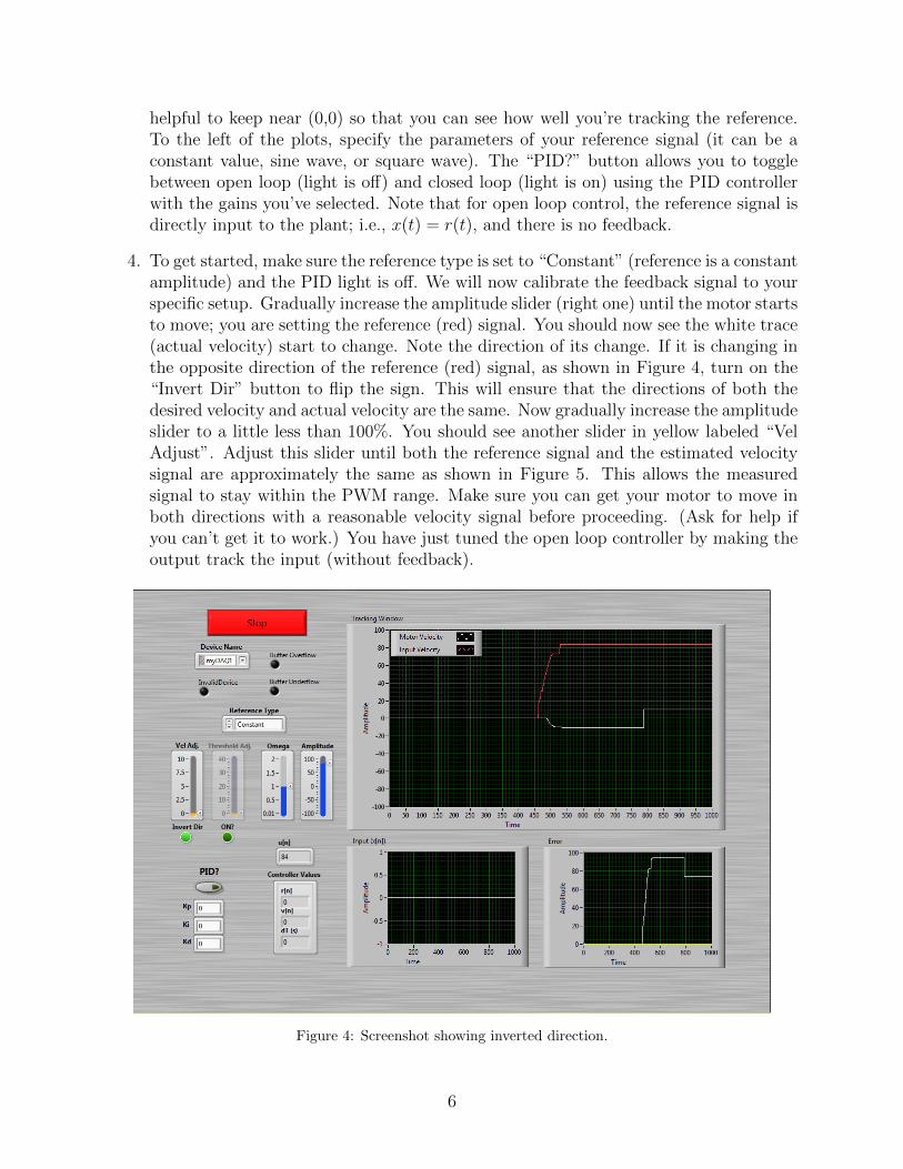
1. Referring to Figures 2 and 3, plug the terminal strip type connector on the PCB intoyour myDAQ by aligning the outer edge pins. Then plug in the battery pack, makingsure that you have the correct polarization. If you are unsure, the LED located nearthe bottom of the board should immediately blink once when unplugging the batterypack if it was plugged in correctly. Plugging it in the wrong way will not do immediatedamage, but could damage the polarized capacitors in left plugged in for many minutes.

4

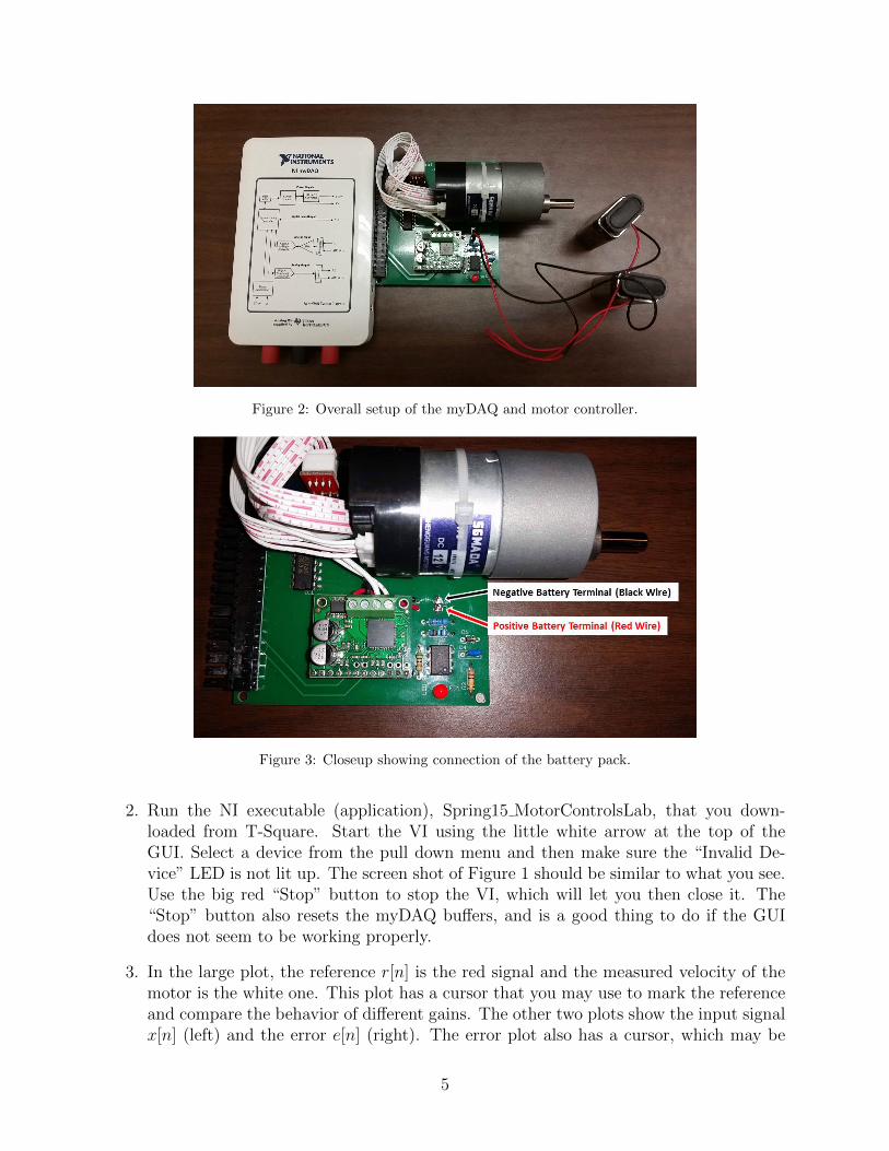
Figure 2: Overall setup of the myDAQ and motor controller.

Figure 3: Closeup showing connection of the battery pack.

2. Run the NI executable (application), Spring15 MotorControlsLab, that you down-loaded from T-Square. Start the VI using the little white arrow at the top of theGUI. Select a device from the pull down menu and then make sure the “Invalid De-vice” LED is not lit up. The screen shot of Figure 1 should be similar to what you see.Use the big red “Stop” button to stop the VI, which will let you then close it. The“Stop” button also resets the myDAQ buffers, and is a good thing to do if the GUIdoes not seem to be working properly.

3. In the large plot, the reference r[n] is the red signal and the measured velocity of themotor is the white one. This plot has a cursor that you may use to mark the referenceand compare the behavior of different gains. The other two plots show the input signalx[n] (left) and the error e[n] (right). The error plot also has a cursor, which may be

5

helpful to keep near (0,0) so that you can see how well you’re tracking the reference.To the left of the plots, specify the parameters of your reference signal (it can be aconstant value, sine wave, or square wave). The “PID?” button allows you to togglebetween open loop (light is off) and closed loop (light is on) using the PID controllerwith the gains you’ve selected. Note that for open loop control, the reference signal isdirectly input to the plant; i.e., x(t) = r(t), and there is no feedback.

4. To get started, make sure the reference type is set to “Constant” (reference is a constantamplitude) and the PID light is off. We will now calibrate the feedback signal to yourspecific setup. Gradually increase the amplitude slider (right one) until the motor startsto move; you are setting the reference (red) signal. You should now see the white trace(actual velocity) start to change. Note the direction of its change. If it is changing inthe opposite direction of the reference (red) signal, as shown in Figure 4, turn on the“Invert Dir” button to flip the sign. This will ensure that the directions of both thedesired velocity and actual velocity are the same. Now gradually increase the amplitudeslider to a little less than 100%. You should see another slider in yellow labeled “VelAdjust”. Adjust this slider until both the reference signal and the estimated velocitysignal are approximately the same as shown in Figure 5. This allows the measuredsignal to stay within the PWM range. Make sure you can get your motor to move inboth directions with a reasonable velocity signal before proceeding. (Ask for help ifyou can’t get it to work.) You have just tuned the open loop controller by making theoutput track the input (without feedback).

Figure 4: Screenshot showing inverted direction.

6

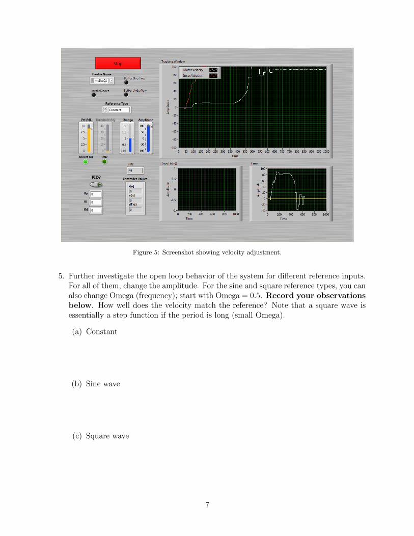
Figure 5: Screenshot showing velocity adjustment.

5. Further investigate the open loop behavior of the system for different reference inputs.For all of them, change the amplitude. For the sine and square reference types, you canalso change Omega (frequency); start with Omega = 0.5. Record your observationsbelow. How well does the velocity match the reference? Note that a square wave isessentially a step function if the period is long (small Omega).

(a) Constant

(b) Sine wave

(c) Square wave

7

Verification #1: Have a lab instructor verify your observations on the pre-vious page and open loop operation with a square wave reference by signingbelow:

Instructor Signature: Time:

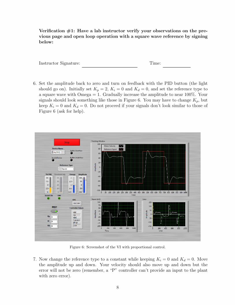
6. Set the amplitude back to zero and turn on feedback with the PID button (the lightshould go on). Initially set Kp = 2, Ki = 0 and Kd = 0, and set the reference type toa square wave with Omega = 1. Gradually increase the amplitude to near 100%. Yoursignals should look something like those in Figure 6. You may have to change Kp, butkeep Ki = 0 and Kd = 0. Do not proceed if your signals don’t look similar to those ofFigure 6 (ask for help).

Figure 6: Screenshot of the VI with proportional control.

7. Now change the reference type to a constant while keeping Ki = 0 and Kd = 0. Movethe amplitude up and down. Your velocity should also move up and down but theerror will not be zero (remember, a “P” controller can’t provide an input to the plantwith zero error).

8

8. With the amplitude non-zero (bigger than 50 is good), change Ki to 1. Watch the errorplot in the lower right as the integral control kicks in and reduces the error. Switchback to a square wave and see how the system performs.

9. Now play around with different values for Kp and Ki (keep Kd = 0 at first) to getmore of a feel for what they do. It is best to initially use a square reference input at alower frequency (Omega < 1) so the motor has time to reach steady state.

10. Find good1 gains. Here are some guidelines:

(a) Start with the proportional term. You won’t be able to get rid of steady-stateerror, but you should see the velocity somewhat mimic the basic shape of thereference without maxing out the control signal x[n] (which goes from -100 to 100).Increasing Kp should decrease the steady state error but increases oscillationswhen the amplitude changes.

(b) Move on to the integral term. This should get rid of steady state error withoutintroducing too many oscillations (happens if Ki is too big). Try to balance Kp

and Ki to get the best performance.

(c) Add a tinyyy bit of derivative term. Do you see what happens with too much?You may be able to increase Kp and Ki after you add a little Kd.

The real world can be kind of messy! Use your judgment as you tune the gains.For a constant reference input of 80, see how low you can keep e[n]. What is|x[n]|? This represents the magnitude of the control effort (smaller is better), andit should not be saturated (i.e., hit ±100%).

(d) Briefly summarize your observations regarding the main effects of Kp, Ki and Kd

for this system and record your minimum e[n].

1Note that there are not 3 unique values that work! Everyone will have a different answer here; do not askif yours is “right.” The point is to make observations, to see how different gains produce different closed-loopbehavior, and to understand the tradeoffs associated with increasing/decreasing each of the three gains.

9

Verification #2: Have a lab instructor verify your observations on the pre-vious page and closed loop operation with constant, square and sine wavereference signals by signing below:

Instructor Signature: Time:

11. For your tuned motor controller, evaluate performance as a function of frequency(Omega) for a sine wave reference. How well do the amplitude and phase track thereference? Summarize your observations below.

12. You have probably noticed that the motor velocity is not proportional to the controlsignal (i.e., it is non-linear). This problem is particularly apparent around zero in thatthe motor doesn’t move if the control signal is too small. Enable the slider “ThresholdAdj”, which sets a threshold for the control signal; i.e., it forces |x(t)| to always begreater than this value. Set this adjustment to give the best performance of your motorfor a sinusoidal reference. How effective is this threshold in overcoming this problem?Does it do better for some frequencies than others?

10