ECDL Module 4 - UCL HEP · PDF fileExcel Part 2 is the second of two workbooks designed to cover the ECDL Module 4 Spreadsheets syllabus. It is one in a series of workbooks designed

ECDL Module 4 Document 354 Version 2

Information Systems EISD

Information Systems

Part of the Education & Information Support Division

Title: Excel 2002 (XP) Part 2

Authors: Rachel Healy and Fiona Strawbridge

Reference: Doc 354 v2

ECDL: Module 4 Spreadsheets (Part 2 of 2)

Date: September 2002

Revisions: Adapted from: Intermediate Excel 5.0 by Rachel Healy.

Updated for Excel 2002 (XP) in August 2002 by Fiona Strawbridge and Tamsin Griffith.

Abstract

Microsoft Excel is a spreadsheet application used for manipulating and calculating numerical data. This workbook is aimed at users who have some knowledge of spreadsheets and of the Excel package, and/or have completed the Excel Part 1 course. It has been designed to accompany the Information Systems Excel Part 2 course (see www.ucl.ac.uk/is/training for course details) and it can be used as a self-paced tutorial. The European Computer Driving Licence (ECDL) Excel Part 2 is the second of two workbooks designed to cover the ECDL Module 4 Spreadsheets syllabus. It is one in a series of workbooks designed to cover the seven modules of the ECDL Syllabus (Version 3.0). For further information, visit the ECDL web pages at www.ucl.ac.uk/is/training/ecdl.htm Pre-requisites It is assumed in this Workbook that you have the requisite keyboard skills and knowledge of a PC including file management, and that you are familiar with the basic uses or Excel including data entry, simple use of formulae and functions, and formatting. If you are unfamiliar with any of these topics, please consult the other workbooks in the series. Please Note Excel 2002 can be accessed from UCL Information Systems (IS) PC Workstations running WTS1. It is assumed in this Workbook that you are a registered user (i.e. you have an IS userid and password) using a PC on the Information Systems WTS Service. Microsoft is a registered trademark and Windows is a trademark of Microsoft Corporation. Screen shots re-printed by permission from Microsoft Corporation.

1 WTS is the Windows Terminal Service which provides a Windows 2000 environment.

Spreadsheets Excel

UCL Information Systems i

Contents

1. Introduction.......................................................................................................................1

2. Data Management With Lists ..........................................................................................2

2.1 To Create a List...........................................................................................................2 2.2 Sorting Records in a List.............................................................................................2 2.3 Simple Filters ..............................................................................................................5

3. Subtotals.............................................................................................................................8

Task Three – Subtotals ...........................................................................................................9

4. The Logical IF Function.................................................................................................10

Task Four – Logical IF .........................................................................................................10

5. Conditional Formatting..................................................................................................11

Task Five – Conditional Formatting.....................................................................................12

6. More Formulae – Absolute References.........................................................................13

6.1 Important Points to Remember .................................................................................13 6.2 The Order of Precedence ..........................................................................................13 6.3 Cell Referencing Systems.........................................................................................13 Task Six – Absolute Referencing .........................................................................................16

7. Working With Names .....................................................................................................17

7.1 Default names ...........................................................................................................17 7.2 To Define a Name Range..........................................................................................17 Task Seven – Using Names ..................................................................................................18

8. Using Comments .............................................................................................................19

8.1 Creating Comments ..................................................................................................19 8.2 To Display Comments ..............................................................................................19 8.3 To Print Comments ...................................................................................................19 Task Eight – Comments........................................................................................................20

9. Paste Special ....................................................................................................................21

Task Nine – Paste Special.....................................................................................................22

10. Working with Workbooks..............................................................................................23

10.1 What are Workbooks?...............................................................................................23 10.2 Selecting in a Workbook...........................................................................................24 10.3 Entering Data ............................................................................................................25 Task Ten - Worksheets .........................................................................................................26 10.4 Managing Worksheets ..............................................................................................27 10.5 Moving and Copying in Workbooks.........................................................................30 10.6 Referencing Cells in Different Sheets.......................................................................31 10.7 Consolidating Data held on Different Sheets............................................................31 Task Eleven – More Worksheets ..........................................................................................32

Excel Part 2

ii UCL Information Systems

11. Templates.........................................................................................................................33

11.1 Creating a Template..................................................................................................33 11.2 To Use a Template ....................................................................................................34 Task Twelve - Templates......................................................................................................35

12. Charts...............................................................................................................................36

12.1 Chart Terms ..............................................................................................................37 12.2 Choosing An Appropriate Chart Type......................................................................38 12.3 Creating Charts using the Chart Wizard ...................................................................39 Task Thirteen – Charting Category Data ..............................................................................44 Task Fourteen – Charting Relationships Between Numerical Data .....................................44 12.4 Changing the Appearance of the Chart .....................................................................45 12.5 Re-sizing Charts & Chart Objects.............................................................................47 12.6 Adding & Removing Data Sets.................................................................................47 Task Fifteen – Amending an Existing Chart ........................................................................48 12.7 Plotting Non-adjacent Cells ......................................................................................49 12.8 Plotting Error Bars ....................................................................................................50 Task Sixteen – Error Bars.....................................................................................................51 12.9 Printing a Chart .........................................................................................................51 Task Seventeen – Printing Charts .........................................................................................53

13. Exercises...........................................................................................................................54

Exercise 1 – Absolute References ........................................................................................54 Exercise 2 – Absolute References ........................................................................................55 Exercise 3 – Absolute References ........................................................................................56 Exercise 4 - Consolidating Data in a Workbook ..................................................................57 Exercise 5 - Revision of Worksheets & Functions ...............................................................58 Exercise 6 - Charts ................................................................................................................59 Exercise 7 - Charts ................................................................................................................60

Part 2 Excel

UCL Information Systems iii

Toolbar Tip

Open

Conventions used in this Workbook

The following table outlines the formatting conventions used in this workbook:

Commands Represented as Commands to input Courier bold Commands output Courier regular Menu commands Buttons to press

Arial Narrow bold

Enter/Return key [↵] Keys to press enclosed in square brackets

e.g. [Ctrl] or [Shift] Key combinations

square brackets with combined keys linked with plus sign e.g. [Ctrl +C] hold down the Control key and press C

Key sequences Press each key enclosed in brackets. e.g. [→] [→] press right arrow key twice in succession

Toolbar Tips Where possible a toolbar shortcut has been provided, shown in a bubble alongside the relevant text. This button can be used instead of the menu method described in the text. How to Use this Workbook This guide can be used as a reference or tutorial document. To facilitate the learning process, a series of practical tasks are contained within the text. You are recommended to try each of these tasks as you progress through the workbook to assist your learning. For further practice and as a means of self-assessment, a number of additional staged exercises, some with solutions, have been included. These should be attempted where recommended. Training Files If you wish to attempt the exercises contained in this document and you are not using a training account it is necessary to download the training files used in this workbook from the IS training web site at: http://www.ucl.ac.uk/is/training/exercises.htm - full instructions on how to do this are provided here.

Part 2 Excel

UCL Information Systems 1

1. Introduction

This workbook is aimed at those who have a good understanding of the basic use of Excel for entering data, performing simple calculations and using simple mathematical functions. It also assumes that you know how to move around a worksheet, control worksheet display, and format a worksheet. These topics are all covered in our Excel Part 1 workbook which you may wish to refer to. We start by looking at how best to organise data in list form in a spreadsheet, and examine some of Excel’s data management tools for sorting, filtering and analysing data. We also look at ways of highlighting data which meet specified criteria, using logical functions and conditional formatting. We review the use of formulae which were introduced in Part 1, and look the use of absolute and named referencing systems for identifying individual cells and ranges of cells. The next brief section looks at the use of comments, which can make your spreadsheets easier to understand (and easier for others to use). This is followed by a short section on paste special which offers flexibility when copying information (not just data, but also formulae, formats and comments) within Excel. The next major section looks at multi-worksheet workbooks which can save time and help you organise similar types of information. This is followed by a brief look at Templates. The final section is devoted to the creating of graphs or chart for presenting numeric data in graphical form.

Excel Part 2

2 UCL Information Systems

2. Data Management With Lists

A list is a series of rows that contain similar data. A list can be thought of as a simple database where rows are records and columns fields. Once a list has been created, it is possible to search for certain items, to sort the data and carry out a variety of analyses.

2.1 To Create a List

When creating a list or database there are some simple guidelines which should be followed: • Avoid having more than one list in a worksheet. • Leave at least one blank row and one column between the list and other data in the

worksheet. • Create column labels (headings) in the first row and place the data immediately below

the headings. • Do not leave empty rows or columns in the list. Excel recognises any list automatically as a database. An example of a list is shown below.

Figure 2-1 - An Excel List or Database

2.2 Sorting Records in a List

The records in a database are arranged in the order in which they were entered. It is possible to sort the records in a list into alphabetical, numeric or date order. You may order records in either ascending or descending order as required. To change the order in which the database is sorted, use one of the different sort methods outlined here:

Toolbar Tip

Ascending Sort

Descending Sort

The column headings are the field names.

The rows are the records in the database

Part 2 Excel


1. Select any cell in the database.

2. From the Data menu choose Sort. The Sort dialogue box is displayed (Figure 2-2). The whole list is automatically selected - the column labels are used to identify the fields.

It is possible to specify up to three Sort Keys. For each key it is possible to specify either an ascending or a descending sort.

2.2.1 To Sort on One Key

1. In the Sort dialogue box, click on the down arrow in the Sort By box and select the required field.

2. Specify either Ascending or Descending and click OK.

Figure 2-2 - Sort Dialogue Box

2.2.2 To Sort on Multiple Keys

1. In the Sort dialogue box, click on the down arrow in the Sort By box and select the required field.

2. Then select the secondary key by selecting a second column/field label in the first Then

By box and specify either Ascending or Descending.

3. To sort on a third field, enter the field name in the remaining Then By box.

4. Click OK. The data in the columns/fields are ordered according to Excel’s sort order:

Numbers Text Logical values Error values Blanks

Use the Options button to sort by day of week or month of year, rather than alphanumerically.

Excel Part 2


Figure 2-3 - Sort on Place and Name

The figure above shows a secondary key sort, the list is sorted on Place first and then on Name within Place. (Notice how the names are ordered within each place group.)

2.2.3 Sorting into Date Order

Note that if you want to sort on date, and the dates are presented in dd/mm/yy format, Excel will automatically recognise that this is a date, and sort appropriately. If, however, your dates are presented as months or days of the week, Excel may not recognise that these are dates, and you may need to use the Options button to reveal the Sort Options dialogue.

Figure 2-4 - Sort Options Dialogue

Task One – Sorting Data in Lists 1. Open the file club.xls from the R:\training.dir\excelp2 folder. 2. Sort the list in ascending order on the field Name. 3. Now re-sort the list in descending order on the field Place and then by the field Name. 4. Save the file.

Primary Sort on Place

Secondary Sort on Name

Part 2 Excel


2.3 Simple Filters

Filters can be created quickly and easily using the AutoFilter. The AutoFilter provides a simple way to find a subset of data in a list. When a list is filtered only those records matching the criteria are displayed. The AutoFilter provides more sophisticated search criteria than are available from within the Data form.

2.3.1 Filter a List Using AutoFilter

1. Select a cell in the list. 2. Select the Data menu, Filter and AutoFilter.

The AutoFilter adds drop-down arrows directly to the column labels in the list, so you can select the item you want to display.

Figure 2-5 - AutoFilter

3. Click on a down arrow to display all the unique items in that field.

4. Select the item you want to find from the list. Rows containing that item will be

displayed, while the others are hidden from view.

2.3.2 To Redisplay All Rows

1. Select the Data menu, Filter and Show All.

Example

Click the pull-down list for the Place column and select Exmoor. All clients who live in Exmoor will be displayed.

2.3.3 To use the Custom Filter

1. Select a cell in the list.

2. Select the Data menu, Filter and AutoFilter.

3. Click on the pull-down arrow in the chosen field to display all the unique items in that field.

Drop down arrows appear in the column label cells

Click on a drop down arrow to display the filter options available

Excel Part 2


4. Select [Custom...]. The Custom AutoFilter dialogue box is displayed.

Figure 2-6 - Custom AutoFilter

5. To enter a criterion, select a condition from the first box and enter a value in the

second. In this example, the is greater than condition has been selected in the first box and then the year 1984.

6. If you want to specify a second set of criteria, select either the And or Or operator and

enter the second set of criteria and click OK. In this example, the is less than or condition has been selected in the second box and then the year 1990.

The records which meet these criteria will be displayed as shown below:

Figure 2-7 - Filtered Data

2.3.4 Specifying Criteria Using Wild Cards

Sometimes we may want to filter our data to match more than one specific item. For example, we may want to find people whose surname begins with the letter S. To carry out these filters we need to use wildcards. Those of you familiar with the Find Tool will recognise the wildcards used by Excel.

Wildcard Matches * Any character or number of characters ? Any single character

Example c* matches cat, canary, cheetah, chimpanzee c?? matches only cat

Note: Wildcards can only be used with text searche; do not use them with values.

Part 2 Excel


2.3.5 Viewing and Editing Filtered Lists

To work with long lists, you may find it easier to freeze areas of the worksheet, for instance, the field names at the top of the list, so that these are always visible. (Window menu, Freeze panes). A filtered list can be edited using the techniques normally used in a worksheet.

Task Two - Filters 1. Add the following records to the club.xls file:

Name Place Date of Birth Year Joined Paid to Date Total Due Hall Exmoor 10/10/70 1997 100.00 150.00 Caruthers Saunton 08/12/69 1997 150.00 150.00 2. Using the Filter tool, list any club member who lives in Coombe Martin. 3. Using the Filter tool, list those records where the members joined in 1984.

4. Using the Filter tool, list those records where the members have paid and the year joined is

between 1990 and 1995 (inclusive).

5. Save the file as club1.xls

Excel Part 2


3. Subtotals

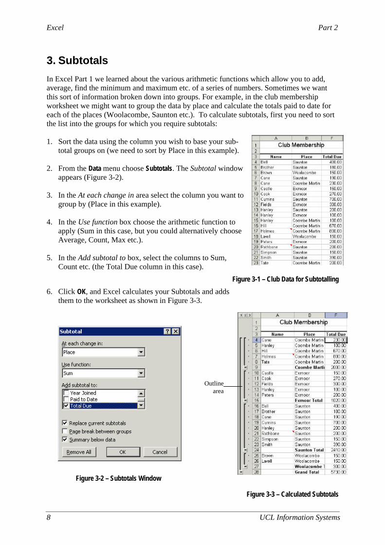
In Excel Part 1 we learned about the various arithmetic functions which allow you to add, average, find the minimum and maximum etc. of a series of numbers. Sometimes we want this sort of information broken down into groups. For example, in the club membership worksheet we might want to group the data by place and calculate the totals paid to date for each of the places (Woolacombe, Saunton etc.). To calculate subtotals, first you need to sort the list into the groups for which you require subtotals: 1. Sort the data using the column you wish to base your sub-

total groups on (we need to sort by Place in this example). 2. From the Data menu choose Subtotals. The Subtotal window

appears (Figure 3-2). 3. In the At each change in area select the column you want to

group by (Place in this example). 4. In the Use function box choose the arithmetic function to

apply (Sum in this case, but you could alternatively choose Average, Count, Max etc.).

5. In the Add subtotal to box, select the columns to Sum,

Count etc. (the Total Due column in this case).

Figure 3-1 – Club Data for Subtotalling

6. Click OK, and Excel calculates your Subtotals and adds them to the worksheet as shown in Figure 3-3.

Figure 3-2 – Subtotals Window

Figure 3-3 – Calculated Subtotals

Outline area

Part 2 Excel


7. Click on the – signs in the Outline area to hide the individual rows and show only the subtotals (Figure 3-4).

Figure 3-4 – Showing Subtotals Only

8. Click on the + signs to reveal the individual rows again.

Task Three – Subtotals 1. Open the club.xls file. 2. Sort the data into ascending order. 3. Produce subtotals based on the Paid to Date column. 4. Now produce subtotals for the Total Due column as well. 5. Use the – signs in the Outline area to collapse the display so that only the rows

containing the subtotals are shown. 6. Save and close the file.

Excel Part 2


4. The Logical IF Function

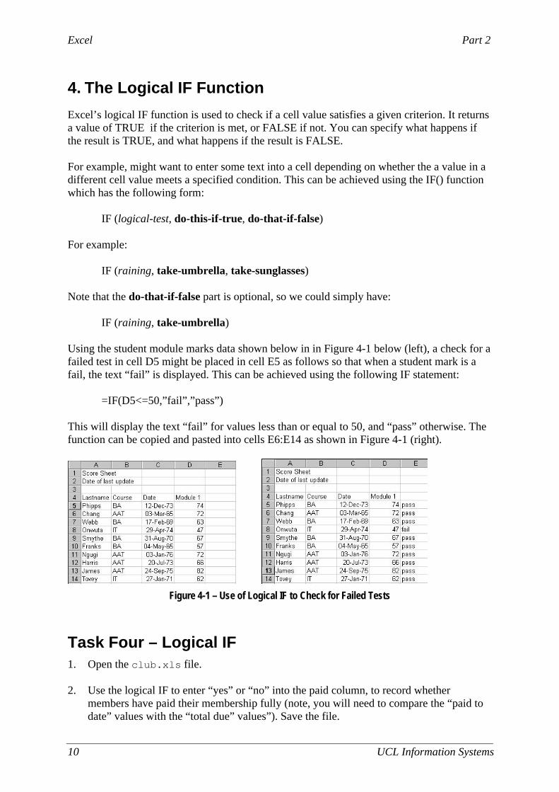
Excel’s logical IF function is used to check if a cell value satisfies a given criterion. It returns a value of TRUE if the criterion is met, or FALSE if not. You can specify what happens if the result is TRUE, and what happens if the result is FALSE. For example, might want to enter some text into a cell depending on whether the a value in a different cell value meets a specified condition. This can be achieved using the IF() function which has the following form: IF (logical-test, do-this-if-true, do-that-if-false) For example: IF (raining, take-umbrella, take-sunglasses) Note that the do-that-if-false part is optional, so we could simply have: IF (raining, take-umbrella) Using the student module marks data shown below in in Figure 4-1 below (left), a check for a failed test in cell D5 might be placed in cell E5 as follows so that when a student mark is a fail, the text “fail” is displayed. This can be achieved using the following IF statement: =IF(D5<=50,”fail”,”pass”) This will display the text “fail” for values less than or equal to 50, and “pass” otherwise. The function can be copied and pasted into cells E6:E14 as shown in Figure 4-1 (right).

Figure 4-1 – Use of Logical IF to Check for Failed Tests

Task Four – Logical IF 1. Open the club.xls file. 2. Use the logical IF to enter “yes” or “no” into the paid column, to record whether

members have paid their membership fully (note, you will need to compare the “paid to date” values with the “total due” values”). Save the file.

Part 2 Excel


5. Conditional Formatting

We have seen how to use the logical IF function to specify what text to display in a cell. However there will be times when you simply want to use formatting (i.e. the appearance of text in a cell) to highlight values in a particular range. For example, you might want to show an overdrawn balance in a financial worksheet in red, or you might want to highlight failed exam marks by displaying them in bold. Excel allows you to do this using “conditional formatting” in which cell values are checked automatically against user-defined criteria. 1. Select the cell(s) you want to apply the conditional formatting to. 2. From the Format menu choose Conditional Formatting. The Conditional Formatting dialogue

displays (Figure 5-1).

Figure 5-1 – Conditional Formatting Dialogue

3. In the Condition area you can specify that the cell value must satisfy one

of a range of conditions using the drop down list (Figure 5-2).

Figure 5-2 – Setting Criteria

4. Enter the required value(s) in the box(es). Note that you can use greater than, :less than, etc. with character as well as numeric data. Greater than “E” would return strings of text starting with F or later in the alphabet.

5. To define the format, click the Format button to display the standard Format Cells

window, and choose an appropriate font colour, style and cell background as required. 6. Click OK to return to the Conditional Formatting window. The formatting choices you

have made will be previewed. 7. Click OK to apply the conditional formatting rules. You should test the formatting by

entering an appropriate value into the cell.

Excel Part 2


Task Five – Conditional Formatting 1. Open the club.xls worksheet in the r:\training.dir\Excelp2 folder. 2. Apply conditional formatting to highlight any members who joined the club after 1990 in

blue. 3. Apply conditional formatting to highlight members whose names occur before “R” in the

alphabet using a yellow background for the cells. 4. Check that the conditional formatting has worked, and save the file.

Part 2 Excel


6. More Formulae – Absolute References

In Excel Part 1 we learned how to enter some simple formulae and functions. Here we will explore these topics in greater detail.

6.1 Important Points to Remember

• Formulae always start with an = (equals) sign • Formulae should always reference the cell address rather than the cell contents. • Place the formula in the cell where the result is to be displayed. Mathematical Operators

+ =A1+A2 addition - =A1-A2 subtraction / =A1/A2 division * =A1*A2 multiplication % 3% percentage ^ =A1^3 exponentiation (to the power of )

6.2 The Order of Precedence

Excel evaluates operators following the conventional rules – it will apply the calculations in a formula in the following order:

BODMAS: Brackets of Division Multiplication Addition Subtraction

( ) brackets first * and / multiplication and division + and - addition and subtraction

Take care to observe these rules when creating your own formulae. The incorrect syntax will result in error.

Formula Result =3+2*4 11 =(3+2)*4 20

6.3 Cell Referencing Systems

The ability to copy formulae from one location to another in a spreadsheet can save you a significant amount of work. Normally, if you copy a formula which involves a cell reference to another location, the cell reference is adjusted relative to its starting point. So, for example, copying a formula which calculates the sum of a column of numbers to an adjacent cell will add up the adjacent column of cells. The formula has updated automatically to reference adjacent cells. This is an example of a relative referencing system.

Excel Part 2


Sometimes we may need to refer to a specific cell location in a worksheet, and so we want that cell reference to remain unchanged, regardless of where the formula is placed. We need a method to fix our cell reference so that it does not update when we copy the formula to another location – we need an absolute cell reference.

6.3.1 Relative References Explained

Cell A3 contains a formula to add the values of the two cells above i.e. =A1+A2. A similar calculation is required in the next column, to add the values in the two cells above the cell B3. To achieve this the formula in cell A3 can be copied from A3 into B3. When the formula is copied, the column reference increments by 1, and the formula becomes =B1+B2.

Figure 6-1 - Relative Referencing

There are times when we may wish to copy the formula in this way, but require the cell reference to stay constant or absolute. Excel provides the facility to override the default, relative referencing system and use absolute references as required.

6.3.2 To Make a Reference Absolute

1. Type a $ sign before both the column letter and the row number of the cell reference. E.g. the relative reference A1 becomes the absolute reference $A$1.

Or use the keyboard short-cut, [F4].

1. In the Formula bar, highlight the cell reference for the cell which is to be made

absolute.

2. Press [F4]. $ signs are automatically placed in front of the column and row references.

Part 2 Excel


6.3.3 To Make a Mixed Reference

If only the columns or the rows are to be absolute, prefix one or the other of these with a $ sign. For example if the column is to be absolute and the row relative A1 becomes $A1, if the row is to be absolute and the column relative A1 becomes A$1. 1. Double click in the cell as if to edit it.

2. Highlight the cell reference to be made absolute and press [F4]. Note

that by pressing [F4] a number of times you cycle through different options for creating a “mixed reference” (see below).

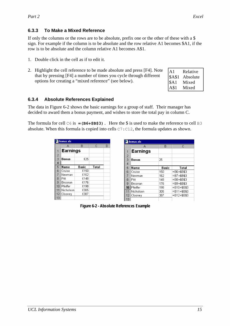
6.3.4 Absolute References Explained

The data in Figure 6-2 shows the basic earnings for a group of staff. Their manager has decided to award them a bonus payment, and wishes to store the total pay in column C. The formula for cell C6 is =(B6+$B$3). Here the $ is used to make the reference to cell B3 absolute. When this formula is copied into cells C7:C12, the formula updates as shown.

Figure 6-2 - Absolute References Example

A1 Relative $A$1 Absolute $A1 Mixed A$1 Mixed

Excel Part 2


Task Six – Absolute Referencing In this exercise you will use a spreadsheet (florist.xls) designed to record sales of fresh flower arrangements. Formulae are required to calculate the total value of each sale (the sum of the Price and the Delivery Charge - this is a constant value) and the number of days which have elapsed since the last Invoice Date (this is also a constant value in the worksheet). 1. Open the file r:\training.dir\excelp2\florist.xls 2. Enter a formula in cell D5 to calculate the Total Cost i.e. Price + Delivery Charge.

What sort of reference should you use to reference the Delivery Charge? 3. Copy the formula to the remaining cells in the column. 4. Enter a formula in cell E5 (under the heading Days Outstanding) to calculate the

number of days since the Invoice Date (D1) i.e. Invoice Date - Date of Sale.

5. Copy the formula to the remaining cells in the column.

6. Enter the labels Average, Minimum, Maximum in cells B22, B23 and B24. 7. Working with the Price column and using the appropriate functions, calculate the

average, minimum and maximum prices, placing the results in cells C22, C23 and C24 respectively.

8. Save the file.

You are now ready to try Exercises 1, 2 and 3.

Part 2 Excel


7. Working With Names

It is easy to lose track of what information particular cells or ranges of cells in a worksheet contain, particularly in a large worksheet. Referring to a cell (or range of cells) by its cell address (e.g. A1, G19, C25:C65) is not very intuitive. To help the user of a worksheet, Excel allows you to create a Name to refer to a cell, a group of cells, a value or a formula .

• A name is easier to remember than a cell reference. • You can use a named reference almost anywhere you might use a regular reference,

including in formulae and dialogue boxes. • Formulae that use names are easier to read and remember than formulae using cell

references. For example, the formula:

=Assets-Liabilities

is clearer to read and understand than the formula:

=F6-G6 • Excel can automatically create names for cells based on row or column titles in your

spreadsheet, or you can enter names for cells or formulae yourself. • If you name a cell which are likely to need to use in an absolute reference, it will

save you from using the $ symbol in the cell reference, as you will simply need to refer to the cell name.

7.1 Default names

By default, every cell has a unique name – the cell address (A1, F4 etc.). When you select a cell, its name appears in the Name Box. It is possible to move directly to a cell location simply by typing the cell name into the Name Box and pressing [Enter].

Figure 7-1 - Name Box

7.2 To Define a Name Range

You can assign a custom name to a cell or cell range to make the worksheet and formulae easier to use and understand. Note that cell names are unique, so you can only use a particular name once in a worksheet. 1. Highlight the range to be named.

2. In the Name Box enter the desired name (note you cannot have spaces in cell names). Or 3. From the Insert menu choose Name, and Define.

The Define Name dialogue box appears.

4. In the Names in Workbook box, type the name you have chosen and click OK.

Name Box

Excel Part 2


The Name Box Once a name has been defined it appears in the Name box. To open the Name box click on the down arrow.

Figure 7-2 - Name Box Drop Down list

7.2.1 To Delete a Named Range

1. Select the Insert menu, Name and Define.

2. Select the name to be deleted from the Define Name dialogue box, click on Delete and OK to finish.

Task Seven – Using Names In this exercise you will use the florist-names.xls spreadsheet which is based on the florist.xls file you used previously. This time you will use named cells and ranges of cells to perform the same calculations. 1. Open the florist-names.xls file from the r:\training.dir\excelp2\ folder. 2. Give the cell containing the Invoice Date(D1) the name InvoiceDate. 3. Give the cell containing the Delivery Charge (D2) the name DeliveryCharge. 4. Give the range of cells containing the purchase date (A5:A20) the name

PurchaseDate. 5. Give the range of cells containing the price (C5:C20) the name Price. 6. Enter a formula in cell D5 to calculate the Total Cost i.e. Price + DeliveryCharge

using Names to refer to the cells. 7. Copy the formula to the remaining cells in the column. 8. Enter a formula in cell E5 (under the heading Days Outstanding) to calculate the

number of days since the Invoice Date (D1) i.e. using Names to refer to the cells.

9. Copy the formula to the remaining cells in the column. 10. Open the florist.xls file from the previous task and check that the results you have

obtained in the two tasks are the same.

11. Save the florist-names.xls file.

Part 2 Excel


8. Using Comments

Comments allow you to add notes to cells in your worksheet. They can be used for example, to communicate with colleagues who will be using the same worksheet, and to remind yourself what a particular value in a cell means, or what a calculation does. When you attach comments to cells in a worksheet, they appear in special dialogue boxes. Comments can also be printed if required.

8.1 Creating Comments

1. Select the cell you want to contain the note. 2. From the Insert menu click Comment.

Figure 8-1 - Comment Box

3. Enter the required text in the Comment box and click outside the box when finished. 4. A small red corner appears in the top right hand corner of a cell that contains a

comment and the comment is displayed as the mouse is moved over the cell. Note that a Reviewing Toolbar appears and contains options for inserting a comment, moving to the next or previous comment, and for showing/hiding one or all comments.

Figure 8-2 - Reviewing Toolbar

8.2 To Display Comments

1. From the View menu click on Comments. Or choose the Show/Hide Comment button .

All the comments in the worksheet will be displayed

8.3 To Print Comments

1. Select the File menu and Page Setup. The Page Setup dialogue box appears. 2. Select the Sheet tab and choose Comments in the Print group. Select either At end of sheet

or As displayed on sheet. 3. Click on the Print button.

Excel Part 2


Task Eight – Comments 1. Open the club.xls file from the R:\training.dir\excelp2 folder. 2. Add the following comment to cell A6 – Resigned with effect from Feb 2001.

3. Add the following comment to cell G3 - If total due is less than total paid

then flag as unpaid

4. What do the notes say in cells A11 and A22? 5. Save the file and close it.

Part 2 Excel


9. Paste Special

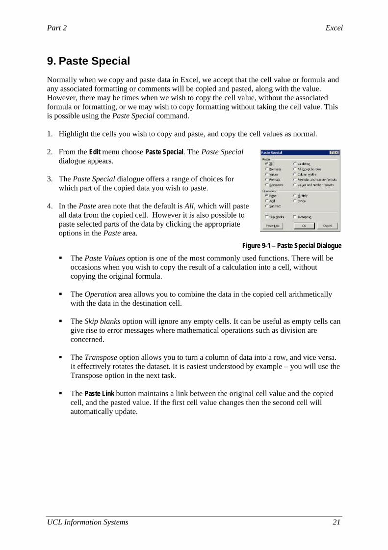
Normally when we copy and paste data in Excel, we accept that the cell value or formula and any associated formatting or comments will be copied and pasted, along with the value. However, there may be times when we wish to copy the cell value, without the associated formula or formatting, or we may wish to copy formatting without taking the cell value. This is possible using the Paste Special command. 1. Highlight the cells you wish to copy and paste, and copy the cell values as normal. 2. From the Edit menu choose Paste Special. The Paste Special

dialogue appears. 3. The Paste Special dialogue offers a range of choices for

which part of the copied data you wish to paste. 4. In the Paste area note that the default is All, which will paste

all data from the copied cell. However it is also possible to paste selected parts of the data by clicking the appropriate options in the Paste area.

Figure 9-1 – Paste Special Dialogue

§ The Paste Values option is one of the most commonly used functions. There will be occasions when you wish to copy the result of a calculation into a cell, without copying the original formula.

§ The Operation area allows you to combine the data in the copied cell arithmetically

with the data in the destination cell. § The Skip blanks option will ignore any empty cells. It can be useful as empty cells can

give rise to error messages where mathematical operations such as division are concerned.

§ The Transpose option allows you to turn a column of data into a row, and vice versa.

It effectively rotates the dataset. It is easiest understood by example – you will use the Transpose option in the next task.

§ The Paste Link button maintains a link between the original cell value and the copied

cell, and the pasted value. If the first cell value changes then the second cell will automatically update.

Excel Part 2


Task Nine – Paste Special 1. Open the module.xls file from the r:\training.dir\excelp2 folder. This file

contains some student marks for four modules. The average marks are shown in row 15, and conditional formatting has been applied to highlight averages below 50 in red.

2. We are going to copy the average data to another part of the worksheet. In cell A17 enter

the text “Average Module Marks”. 3. Make a copy of cells D4 to G4 (the module labels), and paste into cells A18 to D18. 4. Now make a copy of the average marks from cells D15 to G15. Paste the copy into cells

A19:D19. What happens? If you are unsure, examine the contents in the destination cells A18, B18 etc.. You should have realised that Excel has copied the formulae and formats as well as the cell values. This has resulted in error messages as the copied formulae refer to cells which contain text rather than numeric data.

5. You can avoid this problem by using Paste Special to paste just the values which were

copied from cells D15 to G15 into the destination cells. Try this. 6. You may notice that the conditional formatting has not applied to the copied cells. See if

you can use Paste Special to copy the conditional formatting into the destination cells. 7. Finally copy all cells from A4:H14 and this time use the Transpose option from Paste

Special to turn the columns into rows and vice versa. Paste the transposed data into the block of cells starting at cell A21.

Part 2 Excel


10. Working with Workbooks

10.1 What are Workbooks?

In Excel Part 1 we introduced the concept of spreadsheets or worksheets. In this book we will be looking at Workbooks. Workbooks are collections of worksheets stored in the same file. Usually the sheets in a workbook contain related information, such as a departmental budget or a set of experimental results, with each sheet containing the details for a separate budget code or for a set of experiments. By keeping related information together in a workbook, it is easier to manipulate, update and carry out calculations on the data in the worksheets. It is advisable to build a number of smaller related worksheets within a workbook, rather than to create one enormous worksheet. It is very easy to use formulae that refer to other worksheets within the same workbook. • The default workbook contains three sheets - notice the tabs across the bottom of the

document window (Sheet1, Sheet2, Sheet3 etc.). These sheets can be given names to facilitate navigation.

• Sheets can be added or deleted in a workbook. • A single worksheet contains 256 columns and 65,536 rows. • Besides worksheets, a workbook can contain: chart sheets, dialogue box sheets, macro

sheets, and visual basic module sheets.

10.1.1 Moving Between Worksheets in a Workbook

Figure 10-1 - To Select a Sheet

To move between the different sheets in a workbook use the Tab Scrolling buttons.

scrolls to the first sheet tab in the workbook scrolls to the next sheet tab in the workbook

scrolls to the previous sheet tab in the workbook scrolls to the last sheet tab in the workbook

Use the tab scrolling buttons to move between sheets

Click on the sheet tab to select it

Excel Part 2


10.2 Selecting in a Workbook

10.2.1 To select a Sheet

1. Click on the sheet tab to select a sheet.

10.2.2 To Select Multiple Adjacent Sheets

1. Click on the sheet tab of the first sheet you want to select. 2. Hold down the [Shift] key and click on the last Sheet Tab in the required selection.

All the sheets between your first and last click are selected.

Figure 10-2 - Selecting Multiple Contiguous Sheets

10.2.3 To Select Multiple Non-Adjacent Sheets

1. Click on the sheet tab of the first sheet you want to select. 2. Hold down the [Ctrl] key and click on the next sheet you wish to select, repeat this

procedure until all sheets you require have been selected.

Figure 10-3 - Selecting Multiple Non-contiguous Sheets

After you select a group, such as the ones illustrated above, the word [Group] appears in the title bar of the workbook.

10.2.4 To Deselect the Group

1. Click on any Sheet tab.

Or Right-click to reveal the Sheet tab shortcut menu and select Ungroup Sheets.

Click on the first sheet tab and holding down the [Shift] key click on the last sheet tab.

Click on each sheet while holding down the [Ctrl] key.

Part 2 Excel


10.3 Entering Data

10.3.1 To Enter Data in Multiple Sheets

Once you have selected more than one sheet, it is possible to enter the same data in all of the selected sheets simultaneously. This is helpful for setting up several sheets which will store similar information. 1. Select the sheets into which you wish to enter the data.

Notice the word Group appears in the Title bar. 2. Enter your data into the cells as normal. 3. Once the data have been entered, you can click on any of the sheets to see the updated

contents.

10.3.2 Entering Formulae

As with data entry, if the sheet is laid out in the same way, it is possible to enter formulae into several sheets at once. 1. Select the sheets into which you wish to enter the formula.

2. Enter the formula into the cell on the top sheet and copy the formula to the required

cells as normal. 3. Once the formulae have been entered, click in any of the sheets to see the formulae

updated.

Excel Part 2


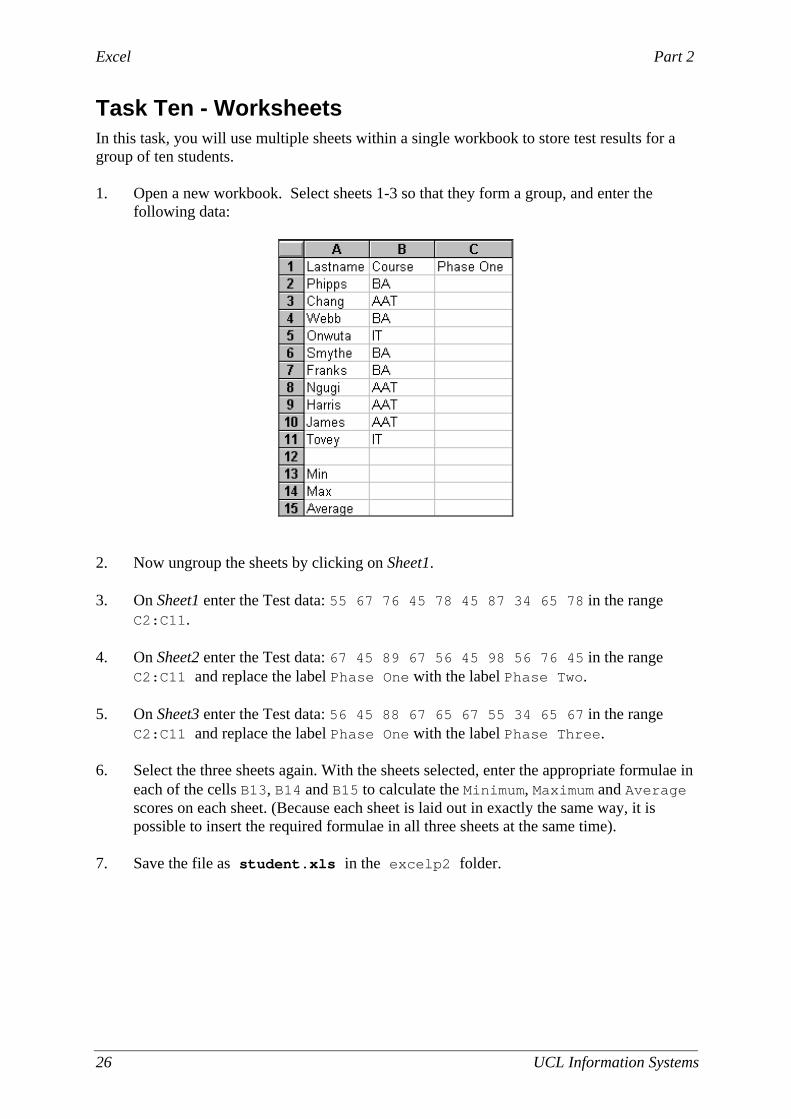
Task Ten - Worksheets In this task, you will use multiple sheets within a single workbook to store test results for a group of ten students. 1. Open a new workbook. Select sheets 1-3 so that they form a group, and enter the

following data:

2. Now ungroup the sheets by clicking on Sheet1. 3. On Sheet1 enter the Test data: 55 67 76 45 78 45 87 34 65 78 in the range

C2:C11.

4. On Sheet2 enter the Test data: 67 45 89 67 56 45 98 56 76 45 in the range C2:C11 and replace the label Phase One with the label Phase Two.

5. On Sheet3 enter the Test data: 56 45 88 67 65 67 55 34 65 67 in the range C2:C11 and replace the label Phase One with the label Phase Three.

6. Select the three sheets again. With the sheets selected, enter the appropriate formulae in each of the cells B13, B14 and B15 to calculate the Minimum, Maximum and Average scores on each sheet. (Because each sheet is laid out in exactly the same way, it is possible to insert the required formulae in all three sheets at the same time).

7. Save the file as student.xls in the excelp2 folder.

Part 2 Excel


10.4 Managing Worksheets

10.4.1 Changing the Default Number of Worksheets

The Excel environment has been set to display three worksheets by default. It is possible to set your own defaults. 1. Select the Tools menu and Options. 2. Select the General tab and specify the number of sheets required in the box Sheets in

New Workbook. The next time a new workbook is opened, the specified number of sheets will appear.

10.4.2 To Insert a New Worksheet

1. Select the Insert menu and Worksheet. A new sheet is inserted in front of the sheet currently selected. Or Use a right mouse click to reveal the shortcut menu and select Insert.

10.4.3 To Delete a Worksheet

1. Select the Sheet to be removed. 2. Select the Edit menu and Delete Sheet

Or Use a right mouse click to reveal the shortcut menu and select Delete.

Figure 10-4 - Sheet Tab Shortcut Menu

Note: If you delete a worksheet, you will not be able to undo this action.

Excel Part 2


10.4.4 Renaming Sheets

1. Select the sheet which you wish to rename.

2. From the Format menu choose Sheet and Rename and type in the new name. Or Use a right mouse-click to reveal the shortcut menu and select Rename. Or Double click on the sheet tab, select the sheet name, and type in the new name. The sheet name can contain up to 31 characters including spaces, but for referencing purposes it is best to limit the number of characters used and avoid spaces. When a sheet is renamed, the sheet tab displays the new name.

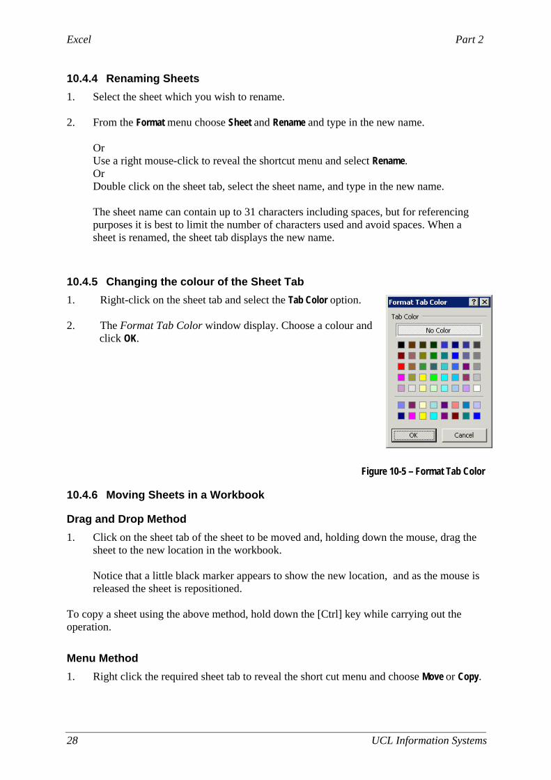
10.4.5 Changing the colour of the Sheet Tab

1. Right-click on the sheet tab and select the Tab Color option. 2. The Format Tab Color window display. Choose a colour and

click OK.

Figure 10-5 – Format Tab Color

10.4.6 Moving Sheets in a Workbook

Drag and Drop Method

1. Click on the sheet tab of the sheet to be moved and, holding down the mouse, drag the sheet to the new location in the workbook.

Notice that a little black marker appears to show the new location, and as the mouse is released the sheet is repositioned.

To copy a sheet using the above method, hold down the [Ctrl] key while carrying out the operation.

Menu Method

1. Right click the required sheet tab to reveal the short cut menu and choose Move or Copy.

Part 2 Excel


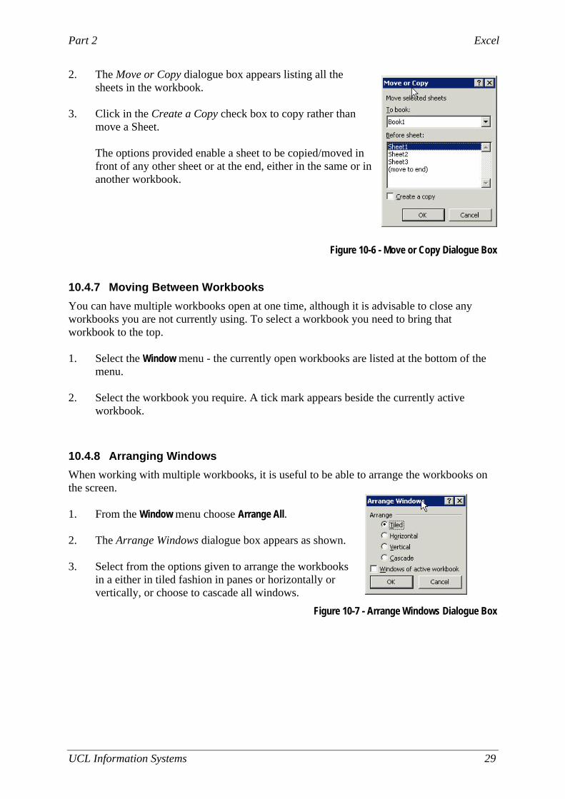
2. The Move or Copy dialogue box appears listing all the sheets in the workbook.

3. Click in the Create a Copy check box to copy rather than

move a Sheet. The options provided enable a sheet to be copied/moved in front of any other sheet or at the end, either in the same or in another workbook.

Figure 10-6 - Move or Copy Dialogue Box

10.4.7 Moving Between Workbooks

You can have multiple workbooks open at one time, although it is advisable to close any workbooks you are not currently using. To select a workbook you need to bring that workbook to the top. 1. Select the Window menu - the currently open workbooks are listed at the bottom of the

menu. 2. Select the workbook you require. A tick mark appears beside the currently active

workbook.

10.4.8 Arranging Windows

When working with multiple workbooks, it is useful to be able to arrange the workbooks on the screen. 1. From the Window menu choose Arrange All. 2. The Arrange Windows dialogue box appears as shown. 3. Select from the options given to arrange the workbooks

in a either in tiled fashion in panes or horizontally or vertically, or choose to cascade all windows.

Figure 10-7 - Arrange Windows Dialogue Box

Excel Part 2


10.5 Moving and Copying in Workbooks

10.5.1 Moving or Copying Data Between Worksheets

1. Select the sheet and data to be moved.

2. Cut the data. 3. Move to the required sheet and cell and paste the data into the new location.

10.5.2 Moving or Copying Data Between Workbooks

To move or copy a sheet to another workbook, ensure both the workbooks are open.

Drag and Drop Method

1. Open the required workbooks and arrange them so that they are visible on the screen as described in Section 10.4.8.

2. Select the sheet to be moved and, holding down the mouse, drag the sheet to the new

location in the required workbook. 3. Notice that a little black marker appears to show the new location, and as the mouse is

released the sheet is repositioned. To copy rather than move, hold down the [Ctrl] key as you carry out the operation. Make sure you release the mouse button before the [Ctrl] key or the sheets will be moved instead of copied.

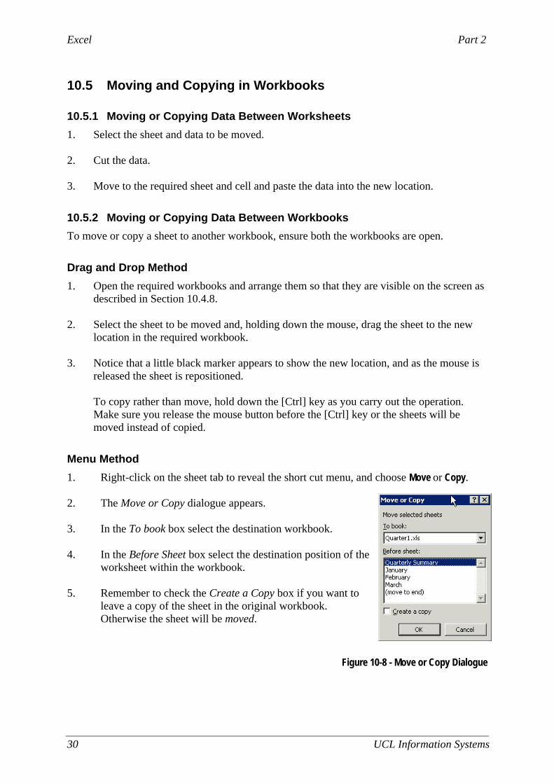
Menu Method

1. Right-click on the sheet tab to reveal the short cut menu, and choose Move or Copy. 2. The Move or Copy dialogue appears. 3. In the To book box select the destination workbook. 4. In the Before Sheet box select the destination position of the

worksheet within the workbook. 5. Remember to check the Create a Copy box if you want to

leave a copy of the sheet in the original workbook. Otherwise the sheet will be moved.

Figure 10-8 - Move or Copy Dialogue

Part 2 Excel


10.6 Referencing Cells in Different Sheets

The different sheets in a workbook should be referred to by including the sheet reference as well as the cell reference in a formula. A sheet reference includes the sheet name followed by an exclamation mark, e.g., Sheet2! refers to Sheet 2. To refer to cell A1 on Sheet2 (when working in any sheet other than Sheet2), the reference would be:

Sheet2!A1

Notice that the exclamation mark separates the sheet reference from the cell reference. If you have named the sheet, simply use the new sheet name (followed by an exclamation mark) and the cell reference. If the sheet name includes spaces you must surround the sheet name with single quotation marks. To refer to cell A1 on a sheet named Budget, the reference would be:

Budget!A1

To refer to cell A1 on a sheet named Annual Budget, the reference would be:

‘Annual Budget’!A1

10.7 Consolidating Data held on Different Sheets

1. On the consolidation or summary sheet, copy or enter the labels you want for the consolidated data.

2. Click a cell that you want to contain consolidated data. 3. Type a formula that includes references to the source cells on each worksheet that

contains data you want to consolidate.

4. Repeat steps 2 and 3 for each cell where you want to consolidate data.

Note To enter a reference in a formula without typing, enter the formula up to the point where you need the reference, and then click the cell on the worksheet. If the cell is on another worksheet, first click the worksheet tab, and then click the cell.

Excel Part 2


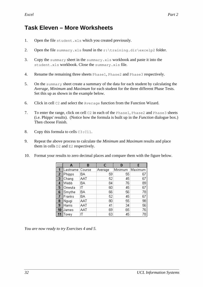
Task Eleven – More Worksheets 1. Open the file student.xls which you created previously.

2. Open the file summary.xls found in the r:\training.dir\excelp2 folder.

3. Copy the summary sheet in the summary.xls workbook and paste it into the

student.xls workbook. Close the summary.xls file. 4. Rename the remaining three sheets Phase1, Phase2 and Phase3 respectively. 5. On the summary sheet create a summary of the data for each student by calculating the

Average, Minimum and Maximum for each student for the three different Phase Tests. Set this up as shown in the example below.

6. Click in cell C2 and select the Average function from the Function Wizard. 7. To enter the range, click on cell C2 in each of the Phase1, Phase2 and Phase3 sheets

(i.e. Phipps' results). (Notice how the formula is built up in the Function dialogue box.) Then choose Finish.

8. Copy this formula to cells C3:C11. 9. Repeat the above process to calculate the Minimum and Maximum results and place

them in cells D2 and E2 respectively. 10. Format your results to zero decimal places and compare them with the figure below.

You are now ready to try Exercises 4 and 5.

Part 2 Excel


11. Templates

There may be certain types of information, formatting or page layout (e.g., page headers and footers) which you frequently include in your worksheets. You can store these standard settings in a Template. When you base a new workbook on an existing template, Excel creates a copy of that template, leaving the original unchanged.

11.1 Creating a Template

1. Create a new worksheet and add any formatting or other information which you want to include in subsequent worksheets.

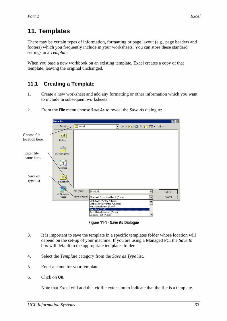
2. From the File menu choose Save As to reveal the Save As dialogue:

Figure 11-1 - Save As Dialogue

3. It is important to save the template in a specific templates folder whose location will

depend on the set-up of your machine. If you are using a Managed PC, the Save In box will default to the appropriate templates folder.

4. Select the Template category from the Save as Type list. 5. Enter a name for your template. 6. Click on OK.

Note that Excel will add the .xlt file extension to indicate that the file is a template.

Save as type list

Enter file name here.

Choose file location here.

Excel Part 2


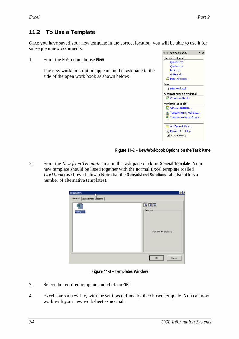
11.2 To Use a Template

Once you have saved your new template in the correct location, you will be able to use it for subsequent new documents. 1. From the File menu choose New.

The new workbook option appears on the task pane to the side of the open work book as shown below:

Figure 11-2 – New Workbook Options on the Task Pane

2. From the New from Template area on the task pane click on General Template. Your

new template should be listed together with the normal Excel template (called Workbook) as shown below. (Note that the Spreadsheet Solutions tab also offers a number of alternative templates).

Figure 11-3 – Templates Window

3. Select the required template and click on OK. 4. Excel starts a new file, with the settings defined by the chosen template. You can now

work with your new worksheet as normal.

Part 2 Excel


Task Twelve - Templates In this task you will create a template in which the first three rows contain user-defined text formatting. You will also personalise the page headers and footers. 1. Create a new workbook. 2. Select the entire worksheet and change the font to Times New Roman size 9. 3. Select row 1 and set the font to Garamond size 14, bold. 4. Adjust the height of row 1 to 20 points. 5. Select row 3 and embolden it. Row 3 is where you would typically place data labels

for data in a list. 6. Create a header (from the File menu choose Page Setup and the Header/Footer tab)

containing the filename in the central section, and a footer containing the date in the right hand section, together with your name in the left hand section.

7. Choose to display gridlines and row and column headings (from Page Setup and the

Sheet tab). 8. Save the file as a template called list.xlt (remember to save it in the Templates

folder), and close the file. Now you can use your template for your next spreadsheet. We will enter a small amount of data into the sheet to test it out. 9. From the File menu choose New. Select your list template

from the New dialogue. 10. Type Test Data into cell A1. 11. Enter the following data into cells A3:B10. The formats

shown here should automatically apply. 12. Save the file as temptest.xls and print it, to check that

your page layout settings (headers, footers and gridlines) have been applied successfully.

Excel Part 2


12. Charts

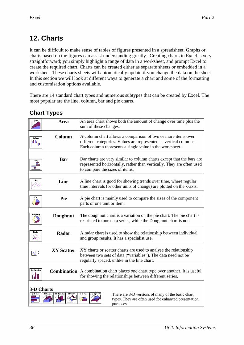
It can be difficult to make sense of tables of figures presented in a spreadsheet. Graphs or charts based on the figures can assist understanding greatly. Creating charts in Excel is very straightforward; you simply highlight a range of data in a worksheet, and prompt Excel to create the required chart. Charts can be created either as separate sheets or embedded in a worksheet. These charts sheets will automatically update if you change the data on the sheet. In this section we will look at different ways to generate a chart and some of the formatting and customisation options available. There are 14 standard chart types and numerous subtypes that can be created by Excel. The most popular are the line, column, bar and pie charts. Chart Types

Area An area chart shows both the amount of change over time plus the

sum of these changes.

Column A column chart allows a comparison of two or more items over different categories. Values are represented as vertical columns. Each column represents a single value in the worksheet.

Bar Bar charts are very similar to column charts except that the bars are represented horizontally, rather than vertically. They are often used to compare the sizes of items.

Line A line chart is good for showing trends over time, where regular

time intervals (or other units of change) are plotted on the x-axis.

Pie A pie chart is mainly used to compare the sizes of the component

parts of one unit or item.

Doughnut The doughnut chart is a variation on the pie chart. The pie chart is restricted to one data series, while the Doughnut chart is not.

Radar A radar chart is used to show the relationship between individual

and group results. It has a specialist use. XY Scatter XY charts or scatter charts are used to analyse the relationship

between two sets of data (“variables”). The data need not be regularly spaced, unlike in the line chart.

Combination A combination chart places one chart type over another. It is useful for showing the relationships between different series.

3-D Charts

There are 3-D versions of many of the basic chart types. They are often used for enhanced presentation purposes.

Part 2 Excel


12.1 Chart Terms

Excel uses a number of different terms to identify the elements of a chart, as detailed below:

Data Points Data points are represented by horizontal bars, lines, columns, sectors points and other figures (data markers). The values from the worksheet determine the size/position of the data markers.

Data Series Data points which come from the same row or column in a worksheet, are grouped in data series.

Value Axis (y axis) The value axis is the numerical scale which shows the value of the data point. It is plotted on the vertical y-axis.

Category Axis (x-axis) The category axis is the line where the various data series are organised, or x-values in x-y charts.

Embedded Charts An embedded chart is a chart displayed in the worksheet alongside the data. When using the ChartWizard this is the default.

Chart Sheets A chart sheet is added to the left of the worksheet that it is based on when you choose to create a chart on a new sheet (Insert menu, Chart, As New Sheet).

The main parts of a chart are identified in the figure below:

Figure 12-1 - The Parts of a Chart

Excel Part 2


12.2 Choosing An Appropriate Chart Type

Where the data you want to present is divided into categories (for example, student numbers by department, or fees by course type), then a bar chart or a column chart is probably a good choice. However, if you want to plot two sets of numeric data against each other in order to analyse the relationship between them (for example, height against age, or traffic density against air pollution), then you will need to use an XY plot, where the x-axis is used to display one variable (age, traffic density) and the y-axis is used for the other variable (height, pollution). In such cases, it is tempting to use a line chart, but this will not be appropriate, as line charts assume that the data on the x-axis are organised into regular intervals or increments. Rather, you should use an XY plot where the x-axis is divided into equal intervals. The difference between the two is illustrated in Figure 12-2 below – look carefully at the x-axis for each chart. The original data show how baby heights vary with age. The age intervals are initially every 3 months, but change to 6 month intervals after 12 months.

Age (months)

Girl height (cm) Boy height (cm)

0 52 54 3 58 61 6 64 68 9 69 74

12 73 79 18 80 90 24 85 95

Figure 12-2 - Line Chart and XY Plot Compared

In the line chart (left) the x-axis starts off with even time intervals, but after 12 months the spacing goes wrong – Excel has plotted each time interval as though it were equally spaced. The plot looks like a pretty straight line. In the XY plot (right) the data have been presented correctly, and it is clear that the relationship is slightly curved. It is clear that using the wrong chart type can result in a misleading interpretation of the data.

Height against age (line chart)

0

20

40

60

80

100

0 3 6 9 12 18 24

Age (months)

Hei

gh

t (c

m)

Girl ave.height (cm)

Boy ave.height (cm)

Height against age (XY plot)

0

20

40

60

80

100

0 6 12 18 24 30

Age (months)

Hei

gh

t (c

m)

Girl ave.height (cm)

Boy ave.height (cm)

Part 2 Excel


12.3 Creating Charts using the Chart Wizard

Charts in Excel are created using the Chart Wizard – a four step wizard which makes the chart creation procedure fairly straightforward. The steps are as follows:

1. Chart Type 2. Chart Source Data 3. Chart Options 4. Chart Location

Once you have selected the data to be charted, the wizard prompts you for the chart type (bar, column, x-y etc.), the range of cells to be plotted, and offers various formatting options. Once the chart has been created, a new Chart Toolbar (Figure 12-3) will appear – this allows further customisation of the chart.

12.3.1 Chart Wizard Step 1 - Chart Type

1. Before activating the Chart Wizard, you should select the data to be plotted, remembering to include the data labels as shown in Figure 12-3.

Figure 12-3 - Selected Data to be Plotted

1. From the Insert menu select Chart.

Step 1 of the Chart Wizard appears as shown in Figure 12-4. In this step you are offered the chart types shown in the figure.

2. Choose a suitable chart type from the left

hand panel, and, if you wish, a subtype from the right hand panel, and press Next to continue to Step 2.

Figure 12-4 - Chart Wizard Step 1 – Selecting Chart Type

Toolbar Tip

ChartWizard

Excel Part 2


12.3.2 Chart Wizard Step 2 - Chart Source Data

The next Wizard Step, Step 2 Chart Source Data, shown in Figure 12-8, has two important tabs; one for controlling the data ranges to be plotted, and the other for selecting what to plot on the x-axis, and which series to show on the y-axis.

Data Range Tab

Figure 12-5 - Chart Wizard Step 2 – Chart Source Data – Data Range Tab Dialogue

The range of cells selected in Step 1 will be displayed in the Data Range tab. This tab also allows you to specify whether the data are organised in rows or columns. By default, the chart is automatically plotted according to the structure of the data. If the data to be plotted has more columns than rows then the default is set to Data Series in Rows (Figure 12-6).

Figure 12-6 - Data Series in Rows

Data points grouped from columns

Data series grouped from rows

Data Range Tab

Series Tab

Part 2 Excel


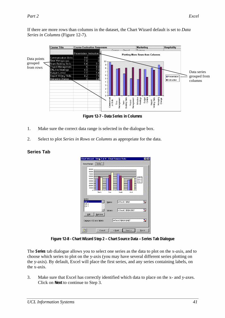
If there are more rows than columns in the dataset, the Chart Wizard default is set to Data Series in Columns (Figure 12-7).

Figure 12-7 - Data Series in Columns

1. Make sure the correct data range is selected in the dialogue box. 2. Select to plot Series in Rows or Columns as appropriate for the data.

Series Tab

Figure 12-8 - Chart Wizard Step 2 – Chart Source Data – Series Tab Dialogue

The Series tab dialogue allows you to select one series as the data to plot on the x-axis, and to choose which series to plot on the y-axis (you may have several different series plotting on the y-axis). By default, Excel will place the first series, and any series containing labels, on the x-axis. 3. Make sure that Excel has correctly identified which data to place on the x- and y-axes.

Click on Next to continue to Step 3.

Data series grouped from columns

Data points grouped from rows

Excel Part 2


12.3.3 Chart Wizard Step 3 - Chart Options

In Step 3 (Figure 12-9) you are presented with many more options for formatting and labelling your chart. Take some time to explore the alternatives offered by the different tabs (Titles, Axes, Gridlines, Legend, Data Labels and Data Table).

Figure 12-9 - Chart Wizard Step 3 – Chart Options

Titles Use to label the chart axes, and to add a title to the chart itself.

Axes Use to customise or remove axis labels.

Legend Choose whether to display a legend, and where to place it.

Gridlines Choose whether to show horizontal and vertical gridlines, and at what intervals.

Data Labels Choose to add labels containing data values to the data points.

Data Table Choose to show the actual data values alongside the chart.

1. When you have fine-tuned the chart to your liking, click on Next to continue to the final

step (Step 4).

Part 2 Excel


12.3.4 Chart Wizard Step 4 - Chart Location

In this step you are asked whether you want to embed the chart in the existing worksheet, or to place it in a separate sheet.

Figure 12-10 - Chart Wizard Step 4 – Chart Location

1. If you select As Object in (the default), the chart appears embedded in the data sheet as

shown in Figure 12-11 – you can move it by clicking in the chart and dragging it to the required location. The chart can also be resized as described in section 12.5. If you choose As New Sheet the chart will appear in a separate window.

Figure 12-11 - Embedded Chart

As new sheet On this sheet

Excel Part 2


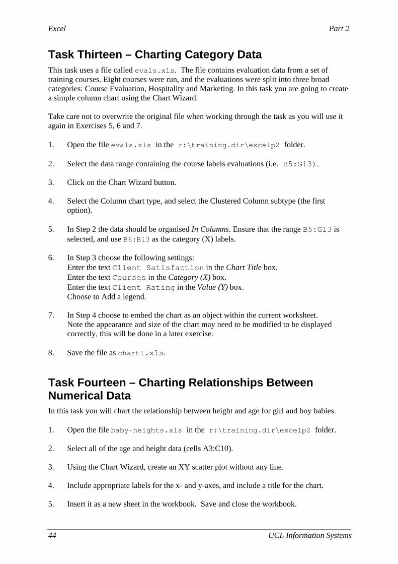
Task Thirteen – Charting Category Data This task uses a file called evals.xls. The file contains evaluation data from a set of training courses. Eight courses were run, and the evaluations were split into three broad categories: Course Evaluation, Hospitality and Marketing. In this task you are going to create a simple column chart using the Chart Wizard. Take care not to overwrite the original file when working through the task as you will use it again in Exercises 5, 6 and 7. 1. Open the file evals.xls in the r:\training.dir\excelp2 folder.

2. Select the data range containing the course labels evaluations (i.e. B5:G13). 3. Click on the Chart Wizard button. 4. Select the Column chart type, and select the Clustered Column subtype (the first

option). 5. In Step 2 the data should be organised In Columns. Ensure that the range B5:G13 is

selected, and use B6:B13 as the category (X) labels. 6. In Step 3 choose the following settings:

Enter the text Client Satisfaction in the Chart Title box. Enter the text Courses in the Category (X) box. Enter the text Client Rating in the Value (Y) box. Choose to Add a legend.

7. In Step 4 choose to embed the chart as an object within the current worksheet. Note the appearance and size of the chart may need to be modified to be displayed correctly, this will be done in a later exercise.

8. Save the file as chart1.xls.

Task Fourteen – Charting Relationships Between Numerical Data In this task you will chart the relationship between height and age for girl and boy babies. 1. Open the file baby-heights.xls in the r:\training.dir\excelp2 folder.

2. Select all of the age and height data (cells A3:C10). 3. Using the Chart Wizard, create an XY scatter plot without any line. 4. Include appropriate labels for the x- and y-axes, and include a title for the chart. 5. Insert it as a new sheet in the workbook. Save and close the workbook.

Part 2 Excel


12.4 Changing the Appearance of the Chart

Once a chart has been created, it is possible to change the settings selected at any of the four steps of its creation (chart type, source data, chart options and location). Formatting options may be accessed in several ways.

12.4.1 Changing the Chart Properties

The Chart Menu 1. Select the chart.

A Chart menu appears on the menu bar. 2. From the Chart menu select Chart Type, Source, Options or Location as required and make the

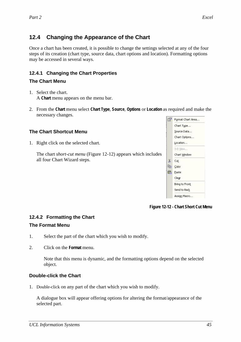
necessary changes. The Chart Shortcut Menu 1. Right click on the selected chart.

The chart short-cut menu (Figure 12-12) appears which includes all four Chart Wizard steps.

Figure 12-12 - Chart Short Cut Menu

12.4.2 Formatting the Chart

The Format Menu 1. Select the part of the chart which you wish to modify.

2. Click on the Format menu.

Note that this menu is dynamic, and the formatting options depend on the selected object.

Double-click the Chart 1. Double-click on any part of the chart which you wish to modify.

A dialogue box will appear offering options for altering the format/appearance of the selected part.

Excel Part 2


12.4.3 The Chart Toolbar

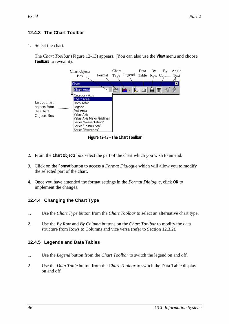
1. Select the chart.

The Chart Toolbar (Figure 12-13) appears. (You can also use the View menu and choose Toolbars to reveal it).

Figure 12-13 - The Chart Toolbar

2. From the Chart Objects box select the part of the chart which you wish to amend. 3. Click on the Format button to access a Format Dialogue which will allow you to modify

the selected part of the chart. 4. Once you have amended the format settings in the Format Dialogue, click OK to

implement the changes.

12.4.4 Changing the Chart Type

1. Use the Chart Type button from the Chart Toolbar to select an alternative chart type. 2. Use the By Row and By Column buttons on the Chart Toolbar to modify the data

structure from Rows to Columns and vice versa (refer to Section 12.3.2).

12.4.5 Legends and Data Tables

1. Use the Legend button from the Chart Toolbar to switch the legend on and off. 2. Use the Data Table button from the Chart Toolbar to switch the Data Table display

on and off.

List of chart objects from the Chart Objects Box

Chart objects Box Format

Chart Type Legend

By Row

By Column

Angle Text

Data Table

Part 2 Excel


12.5 Re-sizing Charts & Chart Objects

1. Select the chart, or the part of the chart, which you wish to resize. 2. A set of handles appear around the selected object. Click and drag a handle to resize

the selected object.

12.6 Adding & Removing Data Sets

Once you have worked through the chart wizard step-by-step, you may well decide that you want to add a further series to the chart. Rather than repeat the whole chart creation process, you can simply select the data to be added, and drag and drop, or copy and paste the data into the chart. Similarly, you can also remove unwanted data from charts without having to remove the entire chart. This will work with both embedded charts and with charts stored on separate sheets.

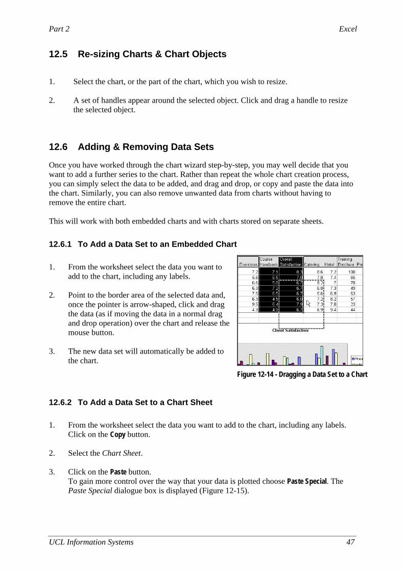
12.6.1 To Add a Data Set to an Embedded Chart

1. From the worksheet select the data you want to

add to the chart, including any labels. 2. Point to the border area of the selected data and,

once the pointer is arrow-shaped, click and drag the data (as if moving the data in a normal drag and drop operation) over the chart and release the mouse button.

3. The new data set will automatically be added to

the chart.

12.6.2 To Add a Data Set to a Chart Sheet

1. From the worksheet select the data you want to add to the chart, including any labels.

Click on the Copy button. 2. Select the Chart Sheet. 3. Click on the Paste button.

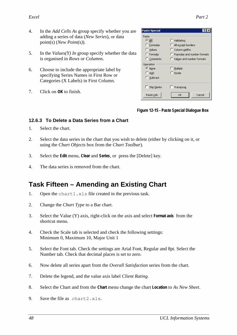
To gain more control over the way that your data is plotted choose Paste Special. The Paste Special dialogue box is displayed (Figure 12-15).

Figure 12-14 - Dragging a Data Set to a Chart

Excel Part 2


4. In the Add Cells As group specify whether you are adding a series of data (New Series), or data point(s) (New Point(s)).

5. In the Values(Y) In group specify whether the data

is organised in Rows or Columns. 6. Choose to include the appropriate label by

specifying Series Names in First Row or Categories (X Labels) in First Column.

7. Click on OK to finish.

Figure 12-15 - Paste Special Dialogue Box

12.6.3 To Delete a Data Series from a Chart

1. Select the chart. 2. Select the data series in the chart that you wish to delete (either by clicking on it, or

using the Chart Objects box from the Chart Toolbar). 3. Select the Edit menu, Clear and Series, or press the [Delete] key. 4. The data series is removed from the chart.

Task Fifteen – Amending an Existing Chart 1. Open the chart1.xls file created in the previous task. 2. Change the Chart Type to a Bar chart.

3. Select the Value (Y) axis, right-click on the axis and select Format axis from the

shortcut menu.

4. Check the Scale tab is selected and check the following settings: Minimum 0, Maximum 10, Major Unit 1

5. Select the Font tab. Check the settings are Arial Font, Regular and 8pt. Select the Number tab. Check that decimal places is set to zero.

6. Now delete all series apart from the Overall Satisfaction series from the chart. 7. Delete the legend, and the value axis label Client Rating. 8. Select the Chart and from the Chart menu change the chart Location to As New Sheet.

9. Save the file as chart2.xls.

Part 2 Excel


12.7 Plotting Non-adjacent Cells

Sometimes you may wish to plot data from different parts of a worksheet. Using the Control [Ctrl] key it is possible to select cell ranges that are not adjacent and to base charts on these ranges, e.g., to plot the hospitality data in our example worksheet whilst using the Course Labels. 1. Select the first range in the worksheet.

2. Hold down the [Ctrl] key and select the second range.

3. Click on the Data Range tab in Step 2 of the Chart Wizard button to check that the

range is correct and proceed as before, completing the remaining steps of the ChartWizard.

Figure 12-16 - Plotting Non-Adjacent Cells

Cells selected using [CTRL] key

Data range corresponding to selected cells

Excel Part 2


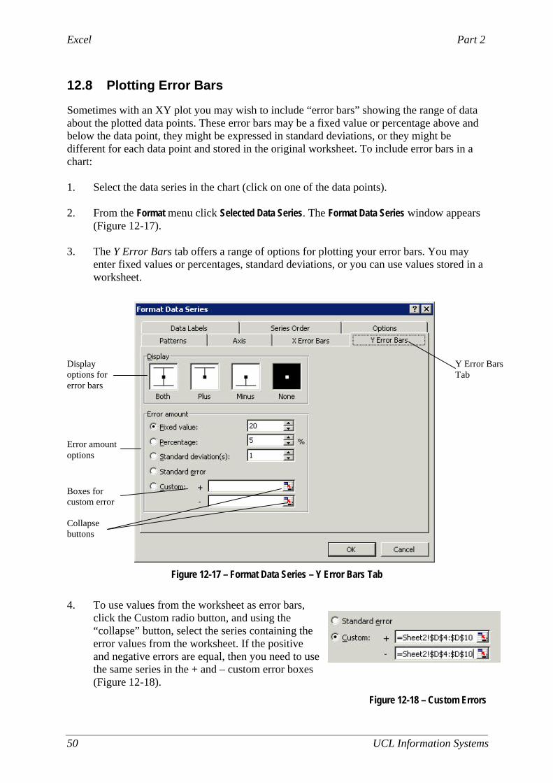
12.8 Plotting Error Bars

Sometimes with an XY plot you may wish to include “error bars” showing the range of data about the plotted data points. These error bars may be a fixed value or percentage above and below the data point, they might be expressed in standard deviations, or they might be different for each data point and stored in the original worksheet. To include error bars in a chart: 1. Select the data series in the chart (click on one of the data points). 2. From the Format menu click Selected Data Series. The Format Data Series window appears

(Figure 12-17). 3. The Y Error Bars tab offers a range of options for plotting your error bars. You may

enter fixed values or percentages, standard deviations, or you can use values stored in a worksheet.

Figure 12-17 – Format Data Series – Y Error Bars Tab

4. To use values from the worksheet as error bars,

click the Custom radio button, and using the “collapse” button, select the series containing the error values from the worksheet. If the positive and negative errors are equal, then you need to use the same series in the + and – custom error boxes (Figure 12-18).

Figure 12-18 – Custom Errors

Display options for error bars

Error amount options

Boxes for custom error Collapse buttons

Y Error Bars Tab

Part 2 Excel


Task Sixteen – Error Bars 1. Open the baby-heights.xls file used in a previous task. 2. Amend the chart to show error bars fixed at 5.5cm above and below each data point

for the Girls data. 3. Now add 6.1 cm error bars for the Boys data. 4. The chart probably looks rather crowded. Amend the scale on the y-axis to display

height values between 40 and 100 cm, with major units of 10cm, and minor units of 5cm.

5. Save the file. 6. Now switch to Sheet 2 – this sheet has individual error measurements for each data

point in columns D (Girls) and E (Boys). 7. Create a new XY chart, this time just displaying the Boy data. Use lines to join the

data points. Place this chart in a separate sheet. 8. Add custom error bars to the chart, based on the error data in column E. 9. Finally, set the colour of the Chart sheet tab to be the same as the colour of the Sheet2

tab, and save the file.

12.9 Printing a Chart

The procedure depends on whether the chart is embedded within a worksheet, or is held as a separate Chart Sheet.

12.9.1 Chart Sheet

1. If a chart is held in a separate sheet, make sure that the sheet containing the chart is selected, and from the File menu choose Print.

12.9.2 Embedded Chart

1. For an embedded chart, to obtain a print-out of the entire worksheet including the chart, make sure that the chart is not selected, and from the File menu choose Print.

2. To obtain a print-out of an embedded chart on its own, select the chart, and from the

File menu choose Print. The Print Dialogue appears (Figure 12-19). 3. In the Print Dialogue the Selected Chart option should be chosen.

Excel Part 2


Figure 12-19 - Print Dialogue

12.9.3 Print Quality & Size

1. Select the chart. From the File menu choose Page Setup and the Chart tab. The Page Setup dialogue box will appear as shown in Figure 12-20. The size and quality of the printed charts can be specified from here.

2. Select the required Chart Size and Print Quality options and click OK.

Figure 12-20 - Page Setup for Printing Charts

Use these options to specify how a chart will be scaled when printed: Use full page Expands the chart to fit the full page. The proportions of the chart are

changed to fill the page. Scale to fit page Expands the chart to fit the full page. The proportions of the chart are

preserved. Custom Scales the chart sheet as it appears on your screen so you can adjust

the chart to any size on the page.

Select required Chart Size. Choose Custom to print the chart as it is displayed in the worksheet.

Select to print in black and white. When cleared, colours print as greyscale on a black-and-white printer.

Selected sheet option

Part 2 Excel


Task Seventeen – Printing Charts 1. Select Sheet1 in the baby-heights.xls file. 2. Print the chart on this worksheet so that the chart and worksheet data are both printed

out on the same sheet of paper. 3. Print the same chart so that the chart alone fills the page. You are now ready to try Exercises 6 and 7.

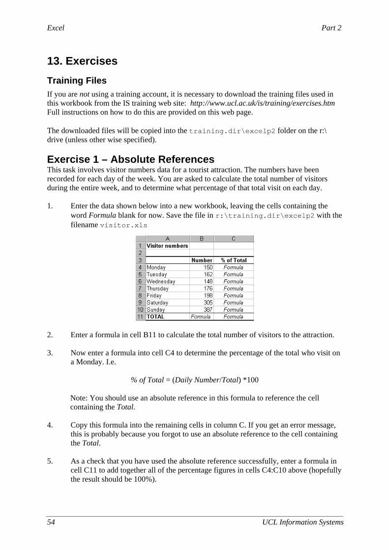
Excel Part 2


13. Exercises

Training Files If you are not using a training account, it is necessary to download the training files used in this workbook from the IS training web site: http://www.ucl.ac.uk/is/training/exercises.htm Full instructions on how to do this are provided on this web page. The downloaded files will be copied into the training.dir\excelp2 folder on the r:\ drive (unless other wise specified). Exercise 1 – Absolute References This task involves visitor numbers data for a tourist attraction. The numbers have been recorded for each day of the week. You are asked to calculate the total number of visitors during the entire week, and to determine what percentage of that total visit on each day. 1. Enter the data shown below into a new workbook, leaving the cells containing the

word Formula blank for now. Save the file in r:\training.dir\excelp2 with the filename visitor.xls

2. Enter a formula in cell B11 to calculate the total number of visitors to the attraction. 3. Now enter a formula into cell C4 to determine the percentage of the total who visit on

a Monday. I.e.

% of Total = (Daily Number/Total) *100

Note: You should use an absolute reference in this formula to reference the cell containing the Total.

4. Copy this formula into the remaining cells in column C. If you get an error message,

this is probably because you forgot to use an absolute reference to the cell containing the Total.

5. As a check that you have used the absolute reference successfully, enter a formula in

cell C11 to add together all of the percentage figures in cells C4:C10 above (hopefully the result should be 100%).

Part 2 Excel


Exercise 2 – Absolute References The train.xls file contains a list of the number of training courses and testing sessions offered by a training provider each month. You are asked to calculate the total number of courses and test sessions during the year, and to determine what percentage of that total take place in each month. 1. Insert a new column between Training Courses and Test Sessions and add the label

% of courses as shown below. Add a further column at the end of the list to store % of tests. Leave the cells containing the word Formula blank for now.

2. Enter the label Total into cell A17. 3. Enter a formula in cell B17 to calculate the total number of training courses over the

year. 4. Now enter a formula into cell C4 to determine the percentage of the total which take

place in January.

% of Courses = (Training Courses/Total) *100 5. Copy this formula into the remaining cells in column C.

If you get an error message, this is probably because you forgot to use an absolute reference to the cell containing the total.

6. As a check that you have used the absolute reference successfully, enter a formula in

cell C17 to add together all of the percentage figures in cells C4:C15 above (hopefully the result should be 100%).

7. Apply the same procedure to calculate the percentage of Tests for each month, and

store the results in cells E4:E15. 8. Again, check that the percentages add up to 100%, using an appropriate formula in

cell E17.

Excel Part 2


Exercise 3 – Absolute References 1. Open the file forecast.xls in the r:\training.dir\excelp2 folder.

This spreadsheet shows the sales value of a number of different items in Year 1. Using these figures and the Annual Sales Growth figures, it is possible to calculate the projected sales figures for each product item for all years up to Year 8.

2. Enter a formula to calculate the projected sales for each of the product groups for years 2 – 8 as shown here:

Projected sales = Sales in previous year + (Sales in previous year * Annual Sales Growth)

3. Move the Annual Sales Growth details i.e. B3:C6 to the left by one column so that they are in line with the other labels. Look at the formulae in Year 2 to see what effect moving the Annual Sales Growth figures has had. What do you notice?

4. Format the Sales figures for each of the years to a currency format with two decimal places.

5. Format the Annual Sales Growth figures to a percentage format with two decimal places.

6. Centre the heading Sales Forecast across the spreadsheet and change the font to Palatino and the point size to 18 pt.

7. Change the size of the heading Annual Sales Growth to 14pt.

8. Insert a border around the Annual Sales Growth details i.e. A2:B6 and shade the cells, using a colour of your choice.

9. Right-align the Year labels.

10. Insert a header with the title Sales Projections and the current date, and a footer with your name.

11. Change the layout to a landscape orientation.

12. Change the top margin to 4cm and centre the worksheet horizontally on the page.

13. Select gridlines and row and column headings.

14. View the spreadsheet in Print Preview and, when you are satisfied with the result, print the worksheet and save the file.

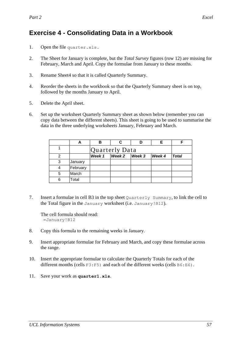
Part 2 Excel


Exercise 4 - Consolidating Data in a Workbook 1. Open the file quarter.xls. 2. The Sheet for January is complete, but the Total Survey figures (row 12) are missing for

February, March and April. Copy the formulae from January to these months. 3. Rename Sheet4 so that it is called Quarterly Summary. 4. Reorder the sheets in the workbook so that the Quarterly Summary sheet is on top,

followed by the months January to April.

5. Delete the April sheet.

6. Set up the worksheet Quarterly Summary sheet as shown below (remember you can copy data between the different sheets). This sheet is going to be used to summarise the data in the three underlying worksheets January, February and March.

A B C D E F 1 Quarterly Data

2 Week 1 Week 2 Week 3 Week 4 Total 3 January 4 February 5 March 6 Total

7. Insert a formulae in cell B3 in the top sheet Quarterly Summary, to link the cell to

the Total figure in the January worksheet (i.e. January!B12). The cell formula should read: =January!B12

8. Copy this formula to the remaining weeks in January.

9. Insert appropriate formulae for February and March, and copy these formulae across the range.

10. Insert the appropriate formulae to calculate the Quarterly Totals for each of the different months (cells F3:F5) and each of the different weeks (cells B6:E6).

11. Save your work as quarter1.xls.

Excel Part 2


Exercise 5 - Revision of Worksheets & Functions In this exercise, you are presented with a workbook which would benefit from splitting into a series of worksheets. The workbook contains sales data covering three months for a small electricals firm. You are asked to reorganise it so that it conforms to basic list management guidelines, and to use the wholesale price of the appliances and the retail price mark up to calculate the retail price and sales value for each month. 1. Open the file provided called elecgds.xls. 2. Now organise the data into worksheets. Use sheet1 to store the wholesale and retail

price information, and name it PriceData. Use one worksheet per month for the sales data, and name the worksheets, Jan, Feb and Mar. Ensure that the layout of these three monthly sheets is identical.

3. Remove any extraneous rows and columns, in order to generate a separate list for each month. You will need to add a heading row for each month i.e. copy the headings Week1 to Week4, Total Units and Sales to each month. Remember that there shouldn’t be any empty rows or columns in a list.

4. In the PriceData sheet, enter formulae to determine the retail price for each of the

products. Remember Absolute References will be necessary if you are going to copy formulae from one cell to another.

Retail Price = Wholesale Price + (Wholesale Price* Mark up) To complete the monthly worksheets, you will need to enter formulae to calculate the number of units sold, and their sales value. (Note - as long as the layout of the monthly sheets is identical, you will be able to enter formulae into all three sheets simultaneously, by selecting them all before typing the formulae). 5. Enter a formula to calculate the Total Units of each product sold per month:

Total Units = Sum of Sales from Week 1 to Week 4.

6. Enter a formula to calculate the Sales value: Sales = Retail Price * Total Units Note – you will have to refer to the Retail Price on the PriceData sheet.

7. Enter a new label Monthly Sales in cell F8 and enter the formula to calculate Monthly Sales for each of the months in cell G8.

Monthly Sales = Sum of Sales

Part 2 Excel


8. Return to the PriceData worksheet, and enter labels January, February and

March in cells A9, A10 and A11 respectively, and in adjacent cells (under a label Monthly Sales) enter formulae to display the Monthly Sales figures from the three worksheets.

9. Add a new label Quarterly Sales at the bottom of the worksheet in cell A13 and enter a formula to calculate the total sales for the quarter in the adjacent cell.

10. Embolden all cells which contain labels. Apply a currency format with two decimal places to all cells containing currency data.

11. Save the worksheet with the name elecgds1.xls Exercise 6 - Charts The following Chart exercises use the file evals.xls which was used in previous Tasks. Take care not to overwrite the original file when working through these exercises. 1. Open the file evals.xls in the r:\training.dir\excelp2 folder.

2. Select the range B5:F7, i.e. the course evaluation data for the Communication Skills

and the Time Management courses.

3. Create a Line chart and select the first format type.

4. Choose to plot the Data Series in rows.

5. Select the Data Labels and choose to Show Value. Choose not to display a legend and do not add a chart title.

6. Select to plot the chart As New Sheet.

7. Save the file as chart3.xls

Excel Part 2


Exercise 7 - Charts Using the same file, evals.xls create a bar chart on a separate sheet to plot the hospitality ratings. 1. Select the non contiguous ranges B5:B13 (Course Names) and H5:I13 (Catering

and Hotel scores). 2. In Step 1 select the first bar chart from the list. 3. In Step 2 check that the range B5:B13,H5:I13 is selected, and that the data series

are in columns, with the first column for category axis labels.

4. Step 3 settings: Enter the text Hospitality Data in the Chart Title box. Enter the text Courses in the Category (X) box. Enter the text Client Rating in the Value (Y) box. Add a legend.

5. In Step 4 choose to insert the chart As New Sheet.

6. Save the file as chart4.xls

Documents

ECDL Module 4 - UCL HEP · PDF fileExcel Part 2 is the second of two workbooks designed to cover the ECDL Module 4 Spreadsheets syllabus. It is one in a series of workbooks designed