Easy over Hard: A Case Study on Deep Learning over Hard: A Case Study on Deep Learning ESEC/FSE’17, September 4-8, 2017, Paderborn, Germany

Easy over Hard: A Case Study on Deep LearningWei Fu, Tim MenziesCom.Sci., NC State, USA

[email protected],[email protected]

ABSTRACTWhile deep learning is an exciting new technique, the bene�ts ofthis method need to be assessed with respect to its computationalcost. �is is particularly important for deep learning since theselearners need hours (to weeks) to train the model. Such long train-ing time limits the ability of (a) a researcher to test the stabilityof their conclusion via repeated runs with di�erent random seeds;and (b) other researchers to repeat, improve, or even refute thatoriginal work.

For example, recently, deep learning was used to �nd whichquestions in the Stack Over�ow programmer discussion forum canbe linked together. �at deep learning system took 14 hours toexecute. We show here that applying a very simple optimizer calledDE to �ne tune SVM, it can achieve similar (and sometimes be�er)results. �e DE approach terminated in 10 minutes; i.e. 84 timesfaster hours than deep learning method.

We o�er these results as a cautionary tale to the so�ware analyt-ics community and suggest that not every new innovation shouldbe applied without critical analysis. If researchers deploy some newand expensive process, that work should be baselined against somesimpler and faster alternatives.

KEYWORDSSearch based so�ware engineering, so�ware analytics, parametertuning, data analytics for so�ware engineering, deep learning, SVM,di�erential evolution

ACM Reference format:Wei Fu, Tim Menzies. 2017. Easy over Hard: A Case Study on Deep Learning.In Proceedings of 2017 11th Joint Meeting of the European So�ware EngineeringConference and the ACM SIGSOFT Symposium on the Foundations of So�-ware Engineering, Paderborn, Germany, September 4-8, 2017 (ESEC/FSE’17),12 pages.DOI: 10.1145/3106237.3106256

1 INTRODUCTION�is paper extends a prior result from ASE’16 by Xu et al. [74](herea�er, XU). XU described a method to explore large programmerdiscussion forums, then uncover related, but separate, entries. �isis an important problem. Modern SE is evolving so fast that theseforums contain more relevant and recent comments on currenttechnologies than any textbook or research article.

In their work, XU predicted whether two questions posted onStack Over�ow are semantically linkable. Speci�cally, XU de�nea question along with its entire set of answers posted on StackOver�ow as a knowledge unit (KU). If two knowledge units are

ESEC/FSE’17, Paderborn, Germany2017. 978-1-4503-5105-8/17/09. . .$15.00DOI: 10.1145/3106237.3106256

semantically related, they are considered as linkable knowledgeunits.

In their paper, they used a convolution neural network (CNN), akind of deep learning method [42], to predict whether two KUs arelinkable. Such CNNs are highly computationally expensive, o�enrequiring network composed of 10 to 20 layers, hundreds of millionsof weights and billions of connections between units [42]. Evenwith advanced hardware and algorithm parallelization, trainingdeep learning models still requires hours to weeks. For example:• XU report that their analysis required 14 hours of CPU.• Le [40] used a cluster with 1,000 machines (16,000 cores) for

three days to train a deep learner.�is paper debates what methods should be recommended to

those wishing to repeat the analysis of XU. We focus on whetherusing simple and faster methods can achieve the results that are cur-rently achievable by the state-of-art deep learning method. Speci�-cally, we repeat XU’s study using DE (di�erential evolution [62]),which serves as a hyper-parameter optimizer to tune XU’s base-line method, which is a conventional machine learning algorithm,support vector machine (SVM). Our study asks:

RQ1: Can we reproduce XU’s baseline results (Word Embedding +SVM)? Using such a baseline, we can compare our methods to thoseof XU.

RQ2: Can DE tune a standard learner such that it outperformsXU’s deep learning method? We apply di�erential evolution to tuneSVM. In terms of precision, recall and F1-score, we observe that thetuned SVM method outperforms CNN in most evaluation scores.

RQ3: Is tuning SVM with DE faster than XU’s deep learningmethod? Our DE method is 84 times faster than CNN.

We o�er these results as a cautionary tale to the so�ware an-alytics community. While deep learning is an exciting new tech-nique, the bene�ts of this method need to be carefully assessed withrespect to its computational cost. More generally, if researchersdeploy some new and expensive process (like deep learning), thatwork should be baselined against some simpler and faster alterna-tives

�e rest of this paper is organized as follows. Section 2 describesthe background and related work on deep learning and parametertuning in SE. Section 3 explains the case study problem and theproposed tuning method investigated in this study, then Section 4describes the experimental se�ings of our study, including researchquestions, data sets, evaluation measures and experimental design.Section 5 presents the results. Section 6 discusses implications fromthe results and the threats to the validity of our study. Section 7concludes the paper and discusses the future work.

Before beginning, we digress to make two points. Firstly, justbecause “DE + SVM” beats deep learning in this application, thisdoes not mean DE is always the superior method for all otherso�ware analytics applications. No learner works best over allproblems [73]– the trick is to try several approaches and select the

arX

iv:1

703.

0013

3v2

[cs

.SE

] 2

4 Ju

n 20

17

ESEC/FSE’17, September 4-8, 2017, Paderborn, Germany Wei Fu, Tim Menzies

one that works best on the local data. Given the low computationalcost of DE (10 minutes vs 14 hours), DEs are an obvious and low-costcandidate for exploring such alternatives.

Secondly, to enable other researchers to repeat, improve, orrefute our results, all our scripts and data are freely available on-line Github1.

2 BACKGROUND AND RELATEDWORK2.1 Why Explore Faster So�ware Analytics?�is section argues that avoiding slow methods for so�ware ana-lytics is an open and urgent issue.

Researchers and industrial practitioners now routinely makeextensive use of so�ware analytics to discover (e.g.) how longit will take to integrate the new code [17], where bugs are mostlikely to occur [54], who should �x the bug [2], or how long it willtake to develop their code [34, 35, 50]. Large organizations likeMicroso� routinely practice data-driven policy development whereorganizational policies are learned from an extensive analysis oflarge data sets collected from developers [7, 65].

But the more complex the method, the harder it is to apply theanalysis. Fisher et al. [20] characterizes so�ware analytics as awork �ow that distills large quantities of low-value data down tosmaller sets of higher value data. Due to the complexities andcomputational cost of SE analytics, “the luxuries of interactivity,direct manipulation, and fast system response are gone” [20]. �eycharacterize modern cloud-based analytics as a throwback to the1960s-batch processing mainframes where jobs are submi�ed andthen analysts wait, wait, and wait for results with “li�le insight intowhat is really going on behind the scenes, how long it will take, orhow much it is going to cost” [20]. Fisher et al. [20] document theissues seen by 16 industrial data scientists, one of whom remarks

“Fast iteration is key, but incompatible with thejobs are submi�ed and processed in the cloud. Itis frustrating to wait for hours, only to realize youneed a slight tweak to your feature set”.

Methods for improving the quality of modern so�ware analyticshave made this issue even more serious. �ere has been continuousdevelopment of new feature selection [25] and feature discover-ing [28] techniques for so�ware analytics, with the most recentones focused on deep learning methods. �ese are all exciting in-novations with the potential to dramatically improve the quality ofour so�ware analytics tools. Yet these are all CPU/GPU-intensivemethods. For instance:• Learning control se�ings for learners can take days to weeks to

years of CPU time [22, 64, 69].• Lam et al. needed weeks of CPU time to combine deep learning

and text mining to localize buggy �les from bug reports [39].• Gu et al. spent 240 hours of GPU time to train a deep learning

based method to generate API usage sequences for given naturallanguage query [24].

Note that the above problem is not solvable by waiting for fasterCPUs/GPUs. We can no longer rely on Moore’s Law [51] to doubleour computational power every 18 months. Power consumption andheat dissipation issues e�ect block further exponential increases to1h�ps://github.com/WeiFoo/EasyOverHard

CPU clock frequencies [38]. Cloud computing environments areextensively monetized so the total �nancial cost of training modelscan be prohibitive, particularly for long running tasks. For example,it would take 15 years of CPU time to learn the tuning parametersof so�ware clone detectors proposed in [69]. Much of that CPUtime can be saved if there is a faster way.

2.2 What is Deep Learning?Deep learning is a branch of machine learning built on multiple lay-ers of neural networks that a�empt to model high level abstractionsin data. According to LeCun et al. [42], deep learning methods arerepresentation-learning methods with multiple levels of represen-tation, obtained by composing simple but non-linear modules thateach transforms the representation at one level (starting with theraw input) into a representation at a higher, slightly more abstractlevel. Compared to the conventional machine learning algorithms,deep learning methods are very good at exploring high-dimensionaldata.

By utilizing extensive computational power, deep learning hasbeen proven to be a very powerful method by researchers in many�elds [42], like computer vision and natural language process-ing [4, 37, 47, 60, 63]. In 2012, Convolution neural networks methodwon the ImageNet competition [37], which achieves half of the errorrates of the best competing approaches. A�er that, CNN became thedominant approach for almost all recognition and detection tasksin computer vision community. CNNs are designed to process thedata in the form of multiple arrays, e.g., image data. According toLeCun et al. [42], recent CNN methods are usually a huge networkcomposed of 10 to 20 layers, hundreds of millions of weights andbillions of connections between units. With advanced hardwareand algorithm parallelization, training such model still need a fewhours [42]. For the tasks that deal with sequential data, like textand speech, recurrent neural networks (RNNs) have been shownto work well. RNNs are found to be good at predicting the nextcharacter or word given the context. For example, Graves et al. [23]proposed to use long short-term memory (LSTM) RNNs to performspeech recognition, which achieves a test set error of 17.7% on thebenchmark testing data. Sutskever et al. [63] used two multiplelay-ered LSTM RNNs to translate sentences in English to French.

2.3 Deep Learning in SEWe study deep learning since, recently, it has a�racted much at-tentions from researchers and practitioners in so�ware commu-nity [15, 24, 39, 52, 68, 70, 71, 74, 77]. �ese researchers applied deeplearning techniques to solve various problems, including defect pre-diction, bug localization, clone code detection, malware detection,API recommendation, e�ort estimation and linkable knowledgeprediction.

We �nd that this work can be divided into two categories:• Treat deep learning as a feature extractor, and then apply other

machine learning algorithms to do further work [15, 39, 68].• Solve problems directly with deep learning [24, 52, 70, 71, 74, 77].

2.3.1 Deep Learning as Pre-Processor. Lam et al. [39] proposedan approach to apply deep neural network in combination withrVSM to automatically locate the potential buggy �les for a given

https://github.com/WeiFoo/EasyOverHard

Easy over Hard: A Case Study on Deep Learning ESEC/FSE’17, September 4-8, 2017, Paderborn, Germany

bug report. By comparing it to baseline methods (Naive Bayes [32],learn-to-rank [76], BugLocator [79]), Lam et al. reported, 16.2-46.4%,8-20.8% and 2.7-20.7% higher top-1 accuracy than baseline methods,respectively [39]. �e training time for deep neural network wasreported from 70 to 122 minutes for 6 projects on a computer with32 cores 2.00GHz CPU, 126 GB memory. However, the runtimeinformation of the baseline methods was not reported.

Wang et al. [68] applied deep belief network to automaticallylearn semantic features from token vectors extracted from the stud-ied so�ware program. A�er applying deep belief network to gener-ate features from so�ware code, Naive Bayes, ADTree and LogisticRegression methods are used to evaluate the e�ectiveness of fea-ture generation, which is compared to the same learners usingtraditional static code features (e.g. McCabe metrics, Halstead’se�ort metrics and CK object-oriented code mertics [13, 26, 31, 45]).In terms of runtime, Wang et al. only report time for generatingsemantics features with deep belief network, which ranged from8 seconds to 32 seconds [68]. However, the time for training andtuning deep belief network is missing. Furthermore, to comparethe e�ectiveness of deep belief network for generating featureswith methods that extract traditional static code features in termsof time cost, it would be favorable to include all the time spent onfeature extraction, including paring source code, token generationand token mapping for both deep belief network and traditionalmethods (i.e., an end-to-end comparison).

Choetkiertikul et al. [15] proposed to apply deep learning tech-niques to solve e�ort estimation problems on user story level.Speci�cally, Choetkiertikul et al. [15] proposed to leverage longshort-term memory (LSTM) to learn feature vectors from the title,description and comments associated with an issue report and af-ter that, regular machine learning techniques, like CART, RandomForests, Linear Regression and Case-Based Reasoning are appliedto build the e�ort estimation models. Experimental results showthat LSTM has a signi�cant improvement over the baseline methodbag-of-words. However, no further information regarding runtimeas well as experimental hardware is reported for both methods andthere is no cost of this deep learning method at all.

2.3.2 Deep Learning as a Problem Solver. White et al. [70, 71]applied recurrent neural networks, a type of deep learning tech-niques, to address code clone detection and code suggestion. �eyreported, the average training time for 8 projects were ranging from34 seconds to 2977 seconds for each epoch on a computer with two3.3 GHz CPUs and each project required at least 30 epochs [70].Speci�cally, for the JDK project in their experiment, it would take25 hours on the same computer to train the models before ge�ingprediction. For the time cost for code suggestions, authors did notmention any related information [71].

Gu et al. [24] proposed a recurrent neural network (RNN) basedmethod, DEEPAPI, to generate API usage sequences for a given natu-ral language query. Compared with the baseline method SWIM [57]and Lucene + UP-Miner [67], DEEPAPI improved the performancesigni�cantly. However, that improvement came at a cost: thatmodel was trained with a Nivdia K20 GPU for 240 hours [24].

XU [74] utilized neural language model and convolution neuralnetwork (CNN) to learn word-level and document-level features topredict semantically linkable knowledge units on Stack Over�ow.

In terms of performance metrics, like precision, recall and F1-score,CNN method was evaluated much be�er than the baseline methodsupport vector machine (SVM). However, once again, that perfor-mance improvement came at a cost: their deep learner required 14hours to train CNN model on a 2.5GHz PC with 16 GB RAM [74].

Yuan et al. [77] proposed a deep belief network based methodfor malware detection on Android apps. By training and testingthe deep learning model with 200 features extracted from staticanalysis and dynamic analysis from 500 sampled Android app, theygot 96.5% accuracy for deep learning method and 80% for onebaseline method, SVM [77]. However, they did not report anyruntime comparison between the deep learning method and otherclassic machine learning methods.

Mou et al. [52] proposed a tree-based convolutional neural net-work for programming language processing, in which a convolutionkernel is designed over programs’ abstract syntax trees to capturestructural information. Results show that their method achieved94% accuracy, which is be�er than the baseline method RBF SVM88.2% on program classi�cation problem [52]. However, Mou etal. [52] did not discuss any runtime comparison between the pro-posed method and baseline methods.

2.3.3 Issues with Deep Learning. In summary, deep learning isused extensively in so�ware engineering community. A commonpa�ern in that research is to:

• Report deep learning’s bene�ts, but not its CPU/GPU cost [15,52, 71, 77];

• Or simply show the cost, without further analysis [24, 39, 68, 70,74].

Since deep learning techniques cost large amount of time and com-putational resources to train its model, one might question whetherthe improvements from deep learning is worth the costs. Are thereany simple techniques that achieve similar improvements with lessresource costs? To investigate how simple methods could improvebaseline methods, we select XU [74] study as a case study. �ereasons are as follows:

• Most deep learning paper’s baseline methods in SE are eithernot publicly available or too complex to implement [39, 70]. XUde�ne their baseline methods precisely enough so others cancon�dently reproduce it locally. XU’s baseline method is SVMlearner, which is available in many machine learning toolboxes.

• Further, it is not yet common practice for deep learning re-searchers in SE community to share their implementations anddata [15, 24, 39, 68, 70, 71], where a tiny di�erence may lead toa huge di�erence in the results. Even though XU do not sharetheir CNN tool, their training and testing data are available on-line, which can be used for our proposed method. Since thesame training and testing data are used for XU’s CNN and ourproposed method, we can compare results of our method to theirCNN results.

• Some studies do not report their runtime and experimental envi-ronment, which makes it harder for us to systematically compareour results with theirs in terms of computational costs [15, 52, 71,77]. XU clearly report their experimental hardware and runtime,which will be easier for us compare our computational costs totheirs.


2.4 Parameter Tuning in SEIn this paper, we use DE as an optimizer to do parameter tuningfor SVM, which achieves results that are competitive with deeplearning. �is section discusses related work on parameter tuningin SE community.

Machine learning algorithms are designed to explore the in-stances to learn the bias. However, most of these algorithms arecontrolled by parameters such as:

• �e maximum allowed depth of decision tree built by CART;• �e number of trees to be built within a Random Forest.

Adjusting these parameters is called hyperparameter optimzia-tion. It is a well well explored approach in other communities [9, 44].However, in SE, such parameter optimization is not a commontask (as shown in the following examples).

In the �eld of defect prediction, Fu et al. [21] surveyed hundredsof highly cited so�ware engineering paper about defect prediction.�eir observation is that most so�ware engineering researchers didnot acknowledge the impact of tunings (exceptions: [43, 64]) anduse the “o�-the-shelf” data miners. For example, Elish et al. [18]compared support vector machines to other data miners for thepurposes of defect prediction. However, the Elish et al. paper makesno mention of any SVM tuning study [18]. More details about theirsurvey refer to [21].

In the �eld of topic modeling, Agrawal et al. [1] investigated theimpact of parameter tuning on Latent Dirichlet Allocation (LDA).LDA is a widely used technique in so�ware engineering �eld to�nd related topics within unstructured text, like topic analytics onStack Over�ow [5] and source code analysis [10]. Agrawal et al.found that LDA su�ers from conclusion instability (di�erent inputorderings can lead to very di�erent results) that is a result of poorchoice of the LDA control parameters [1]. Yet, in their survey ofLDA use in SE, they found that very few researchers (4 out of 57papers) explored the bene�ts of parameter tuning for LDA.

One troubling trend is that, in the few SE papers that performtuning, they do so using methods heavily deprecated in the ma-chine learning community. For example, two SE papers that usetuning [43, 64], apply a simple grid search to explore the potentialparameter space for optimal tunings (such grid searchers run onefor-loop for each parameter being optimized). However, Bergstraet al. [9] and Fu et al. [22] argue that random search methods (e.g.the di�erential evolution algorithm used here) are be�er than gridsearch in terms of e�ciency and performance.

3 METHOD3.1 Research Problem�is section is an overview of the the task and methods used byXU. �eir task was to predict relationships between two knowledgeunits (questions with answers) on Stack Over�ow. Speci�cally, XUdivided linkable knowledge unit pairs into 4 di�erence categoriesnamely, duplicate, direct link, indirect link and isolated, based on itsrelatedness. �e de�nition of these four categories are shown inTable 1 [74]:

In that paper, XU provided the following two methods as base-lines [74]:

Table 1: Classes of Knowledge Unit Pairs.Class Description

Duplicate �ese two knowledge units are addressing thesame question.

Direct link One knowledge unit can help to answer thequestion in the other knowledge unit.

Indirect linkOne knowledge provides similar information tosolve the question in the other knowledge unit,but not a direct answer.

Isolated �ese two knowledge units discuss unrelatedquestions.

• TF-IDF + SVM: a multi-class SVM classi�er with 36 textualfeatures generated based on the TF and IDF values of the wordsin a pair of knowledge units.

• Word Embedding + SVM: a multi-class SVM classi�er with wordembedding generated by the word2vec model [47].

Both of these two baseline methods are compared against theirproposed method, Word Embedding + CNN.

In this study, we select Word Embedding + SVM as the baselinebecause it uses word embedding as the input, which is the same asthe Word Embedding + CNN method by XU.

3.2 Learners and�eir ParametersSVM has been proven to be a very successful method to solve textclassi�cation problem. A SVM seeks to minimize misclassi�cationerrors by selecting a boundary or hyperplane that leaves the max-imum margin between positive and negative classes (where themargin is de�ned as the sum of the distances of the hyperplanefrom the closest point of the two classes [29]).

Like most machine learning algorithms, there are some parame-ters associated with SVM to control how it learns. In XU’s experi-ment, they used a radial-bias function (RBF) for their SVM kerneland set γ to 1/k , where k is 36 for TF-IDF + SVM method and200 for Word Embedding + SVM method. For other parameters,XU mentioned that grid search was applied to optimize the SVMparameters, but no further information was disclosed.

For our work, we used the SVM module from Scikit-learn [55], aPython package for machine learning, where the parameters shownin Table. 2 are selected for tuning. Parameter C is to set the amountof regularization, which controls the tradeo� between the errorson training data and the model complexity. A small value for Cwill generate a simple model with more training errors, while alarge value will lead to a complicated model with fewer errors.Kernel is to introduce di�erent nonlinearities into the SVM modelby applying kernel functions on the input data. Gamma de�neshow far the in�uence of a single training example reaches, withlow values meaning ‘far’ and high values meaning ‘close’. coef0 isan independent parameter used in sigmod and polynomial kernelfunction.

As to why we used the “Tuning Range” shown in Table 2, and notsome other ranges, we note that (a) those ranges include the defaultsand also XU’s values; (b) the results presented below show that byexploring those ranges, we achieved large gains in the performanceof our baseline method. �is is not to say that larger tuning ranges


Table 2: List of Parameters Tuned by�is Paper.Parameters Default Xue et al. Tuning Range Description

C 1.0 unknown [1, 50] Penalty parameter C of the error term.kernel ‘rbf’ ‘rbf’ [‘liner’, ‘poly’, ‘rbf’, ‘sigmoid’] Specify the kernel type to be used in the algorithms.gamma 1/n features 1/200 [0, 1] Kernel coe�cient for ‘rbf’, ‘poly’ and ‘sigmoid’.coef0 0 unknown [0, 1] Independent term in kernel function. It is only used in ‘poly’ and ‘sigmoid’.

might not result in greater improvements. However, for the goalsof this paper (to show that tuning baseline method does ma�er),exploring just these ranges shown in Table 2 will su�ce.

3.3 Learning Word EmbeddingLearning word embeddings refers to �nd vector representationsof words such that the similarities between words can be capturedby cosine similarity of corresponding vector representations. It isbeen shown that the words with similar semantic and syntactic arefound closed to each other in the embedding space [47].

Several methods have been proposed to generate word embed-dings, like skip-gram [47], GloVe [56] and PCA on the word co-occurrence matrix [41]. To replicate XU work, we used the contin-uous skip-gram model (word2vec), which is a unsupervised wordrepresentation learning method based on neural networks and alsoused by XU [74].

�e skip-gram model learns vector representations of words bypredicting the surrounding words in a context window. Given a sen-tence of wordsW = w1,w2,…,wn , the objective of skip-gram modelis to maximize the the average log probability of the surroundingwords:

1n

n∑i=1

∑−c≤j≤c, j,0

loдp(wi+j |wi )

where c is the context window size and wi+j and wi representsurrounding words and center word, respectively. �e probabilityof p(wi+j |wi ) is computed according to the so�max function:

p(wO |wI ) =exp(vTwO

vwI )∑ |W |w=1 exp(v

TwvwI )

where vwI and vwO are the vector representations of the input andoutput vectors of w , respectively.

∑ |W |w=1 exp(v

TwvwI ) normalizes

the inner product results across all the words. To improve thecomputation e�ciency, Mikolove et al. [47] proposed hierachicalso�max and negative sampling techniques. More details can befound in Mikolove et al.’s study [47].

Skip-gram’s parameters control how that algorithm learns wordembeddings. �ose parameters include window size and dimen-sionality of embedding space, etc. Zucoon et al. [80] found thatembedding dimensionality and context window size have no con-sistent impact on retrieval model performance. However, Yang etal. [75] showed that large context window and dimension sizesare preferable to improve the performance when using CNN tosolve classi�cation tasks for Twi�er. Since this work is to compareperformance of tuning SVM with CNN, where skip-gram modelis used to generate word vector representations for both of thesemethods, tuning parameter of skip-gram model is beyond the scopeof this paper (but we will explore it in future work).

1. Given a model (e.g., SVM) with n decisions (e.g., n = 4), TUNER callsSAMPLE N = 10 ∗ n times. Each call generates one member of thepopulation popi∈N .2. TUNER scores each popi according to various objective scores o. Inthe case of our tuning SVM, the objective o is to maximize F1-score3. TUNER tries to each replace popi with a mutantm built using Storn’sdi�erential evolution method [62]. DE extrapolates between three othermembers of population a, b, c . At probability p1, for each decisionak ∈ a, then mk = ak ∨ (p1 < rand() ∧ (bk ∨ ck )).4. Each mutant m is assessed by calling EVALUATE(model, prior=m);i.e. by seeing what can be achieved within a goal a�er �rst assumingthat prior =m.5. To test if the mutant m is preferred to popi , TUNER simply compareSCORE(m) with SCORE(popi ). In case of our tuning SVM, the one withhigher score will be kept.6. TUNER repeatedly loops over the population, trying to replace itemswith mutants, until new be�er mutants stop being found.7. Return the best one in the population as the optimal tunings.

Figure 1: Procedure TUNER: strives to �nd “good” tuningswhich maximizes the objective score of the model on train-ing and tuning data. TUNER is based on Storn’s di�erentialevolution optimizer [62].

To train our word2vec model, 100, 000 knowledge units taggedwith “java” from Stack Over�ow posts table (include titles, ques-tions and answers) are randomly selected as a word corpus2. A�erapplying proper data processing techniques proposed by XU, likeremove the unnecessary HTML tags and keep short code snippetsin code tag, then �t the corpus into gensim word2vec module [58],which is a python wrapper over original word2vec package.

When converting knowledge units into vector representations,for each word wi in the post processed knowledge unit (includingtitle, question and answers), we query the trained word2vec modelto get the corresponding word vector representation vi . �en thewhole knowledge unit with s words is converted to vector repre-sentation by element-wise addition, Uv = vi ⊕ v2 ⊕ ... ⊕ vs . �isvector representation is used as the input data to SVM.

3.4 Tuning AlgorithmA tuning algorithm is an optimizer that drives the learner to explorethe optimal parameter in a given searching space. According to ourliterature review, there are several searching algorithms used inSE community:simulated annealing [19, 46]; various genetic algo-rithms [3, 27, 30] augmented by techniques such as di�erential evo-lution [1, 12, 21, 22, 62], tabu search and sca�er search [6, 16, 49]; par-ticle swarm optimization [72]; numerous decomposition approaches

2Without further explanation, all the experiment se�ings, including learner algorithms,training/testing data split, etc, strictly follow XU’s work.


that use heuristics to decompose the total space into small prob-lems, then apply a response surface methods [36]; NSGA-II [78]andNSGA-III [48].

Of all the mentioned algorithms, the simplest are simulatedannealing (SA) and di�erential evolution (DE), each of which canbe coded in less than a page of some high-level scripting language.Our reading of the current literature is that there are more advocatesfor di�erential evolution than SA. For example, Vesterstrom and�omsen [66] found DE to be competitive with particle swarmoptimization and other GAs. DEs have already been applied beforefor parameter tuning in SE community to do parameter tuning (e.g.see [1, 14, 21, 22, 53]) . �erefore, in this work, we adopt DE as ourtuning algorithm and the main steps in DE is described in Figure 1.

4 EXPERIMENTAL SETUP4.1 Research�estionsTo systematically investigate whether tuning can improve the per-formance of baseline methods compared with deep learning method,we set the following three research questions:• RQ1: Can we reproduce XU’s baseline results (Word Embedding +

SVM)?• RQ2: Can DE tune a standard learner such that it outperforms

XU’s deep learning method?• RQ3: Is tuning SVM with DE faster than XU’s deep learning

method?

RQ1 is to investigate whether our implementation of Word Em-bedding + SVM method has the similar performance with XU’sbaseline, which makes sure that our following analysis can be gen-eralized to XU’s conclusion. RQ2 and RQ3 lead us to investigatewhether tuning SVM comparable with XU’s deep learning fromboth performance and cost aspects.

4.2 Dataset and Experimental DesignOur experimental data comes from Stack Over�ow data dump ofSeptember 20163, where the posts table includes all the questionsand answers posted on Stack Over�ow up to date and the postlinkstable describes the relationships between posts, e.g., duplicate andlinked. As mentioned in Section 3.1, we have four di�erent typesof relationships in knowledge unit pairs. �erefore, linked type isfurther divided into indirectly linked and directly linked. Overall,four di�erent types of data are generated according the followingrules [74]:• Randomly select a pair of posts from the postlinks table, if the

value in PostLinkTypeId �eld for this pair of posts is 3, then thispair of posts is duplicate posts. Otherwise they’re directly linkedposts.

• Randomly select a pair of posts from the posts table, if this pairof posts is linkable from each other according to postlinks tableand the distance between them are greater than 2 (which meansthey are not duplicate or directly linked posts), then this pair ofposts is indirectly linked. If they’re not linkable, then this pairof posts is isolated.

3h�ps://archive.org/details/stackexchange

Word2Vec

WordEmbeddings

Lookup TestingKUvectors Predict Results

TrainingKUpairs NewTrainingKUvectors TuningKUvectors

Lookup

SVM

100,000KUtexts

Train

EvaluateTrain

SVMParameters

DE

BestTuningsTrain

TrainWord2Vec

TrainLearner

TestLearner

ParameterTuning

TestingKUpairs

Figure 2: �e Overall Work�ow of Building KnowledgeUnits Predictor with Tuned SVM

In this work, we use the same training and testing knowledgeunit pairs as XU [74]4, where 6,400 pairs of knowledge units fortraining and 1,600 pairs for testing. And each type of linked knowl-edge units accounts for 1/4 in both training and testing data. �ereasons that we used the same training and testing data as XU are:• It is to ensure that performance of our baseline method is as

closed to XU’s as possible.• Since deep learning method is way complicated compared to

SVM and a li�le di�erence in implementations might lead todi�erent results. To fairly compare with XU’s result, we can usethe performance scores of CNN method from XU’s study [74]without any implementation bias introduced.For training word2vec model, we randomly select 100,000 knowl-

edge units (title, question body and all the answers) from posts tablethat are related to “java”. A�er that, all the training/tuning/testingknowledge units used in this paper are converted into word embed-ding representations by looking up each word in wrod2vec modelas described in Section 3.3.

As seen in Figure 2, instead of using all the 6,400 knowledge unitsas training data, we split the original training data into new trainingdata and tuning data, which are used during parameter tuningprocedure for training SVM and evaluating candidate parameterso�ered by DE. A�erwards, the new training data is again ��edinto the SVM with the optimal parameters found by DE and �nallythe performance of the tuned SVM will be evaluated on the testingdata.

To reduce the potential variance caused by how the original train-ing data is divided, 10-fold cross-validation is performed. Speci�cally,each time one fold with 640 knowledge units pairs is used as thetuning data, and the remaining folds with 5760 knowledge unitsare used as the new training data, then the output SVM model willbe evaluated on the testing data. �erefore, all the performancescores reported below are averaged values over 10 runs.

In this study, we use Wilcoxon single ranked test to statisticallycompare the di�erences between tuned SVM and untuned SVM.Speci�cally, the Benjamini-Hochberg (BH) adjusted p-value is usedto test whether a di�erence is statistically signi�cant at the level of0.05 [8]. To measure the e�ect size of performance scores between4h�ps://github.com/XBWer/ASEDataset

https://github.com/XBWer/ASEDataset


tuned SVM and untuned SVM, we compute Cli�’s δ that is a non-parametric e�ect size measure [59]. As Romano et al. suggested,we evaluate the magnitude of the e�ect size as follows: negligible(|δ | < 0.147 ), small (0.147 < |δ | < 0.33), medium (0.33 < |δ | <0.474 ), and large (0.474 ≤ |δ |) [59].

4.3 Evaluation MetricsWhen evaluating the performance of tuning SVM on the multi-class linkable knowledge units prediction problem, consistent withXU [74], we use accuracy, precision, recall and F1-score as theevaluation metrics.

Table 3: Confusion Matrix.Classi�ed as

C1 C2 C3 C4

Actu

al

C1 c11 c12 c13 c14C2 c21 c22 c23 c24C3 c31 c32 c33 c34C4 c41 c42 c43 c44

Given a multi-classi�cation problem with true labels C1, C2, C3and C4, we can generate a confusion matrix like Table 3, where thevalue of cii represents the number of instances that are correctlyclassi�ed by the learner for class Ci .

Accuracy of the learner is de�ned as the number of correctlyclassi�ed knowledge units over the total number of knowledgeunits, i.e.,

accuracy =∑i cii∑

i∑j ci j

where∑i∑j ci j is the total number of knowledge units. For a given

type of knowledge units, Cj , the precision is de�ned as probabilityof knowledge units pairs correctly classi�ed as Cj over the numberof knowledge unit pairs classi�ed as Cj and recall is de�ned as thepercentage of all Cj knowledge unit pairs correctly classi�ed. F1-score is the harmonic mean of recall and precision. Mathematically,precision, recall and F1-score of the learner for class Cj can bedenoted as follows:

prec j = precisionj =c j j∑i ci j

pdj = recallj =c j j∑i c ji

F1j = 2 ∗ pdj ∗ prec j/(pdj + prec j )Where

∑i ci j is the predicted number of knowledge units in class

Cj and∑i c ji is the actual number of knowledge units in class Cj .

Recall from Algorithm 1 that we call di�erential evolution oncefor each optimization goal. Generally, this goal depends on whichmetric is most important for the business case. In this work, weuse F1 to score the candidate parameters because it controls thetrade-o� between precision and recall, which is also consistent withXU [74] and is also widely used in so�ware engineering communityto evaluate classi�cation results [21, 33, 46, 68].

5 RESULTSIn this section, we present our experimental results. To answerresearch questions raised in Section 4.1, we conducted two experi-ments:

Figure 3: Score Delta between Our SVM with XU’s SVMin [74] in Terms of Precision, Recall and F1-score. PositiveValues Mean Our SVM is Better than XU’s SVM in Terms ofDi�erent Measures; Otherwise, XU’s SVM is better.

• Compare performance of Word Embedding + SVM method inXU [74] and our implementation;• Compare performance of our tuning SVM with DE method with

XU’s CNN deep learning method.Since we used the same training and testing data sets provided byXU [74] and conducted our experiment in the same procedure andevaluated methods using the performance measures, we simplyused the results reported in the work by XU [74] for the perfor-mance comparison.

RQ1: Can we reproduce XU’s baseline results (Word Em-bedding + SVM)?

�is �rst question is important to our work since, without theoriginal tool released by XU, we need to insure that our reimple-mentation of their baseline method (WordEmbedding + SVM) has asimilar performance to their work. Accordingly, we carefully followXU’s procedure [74]. We use the SVM learner from scikit-learnwith the se�ing γ = 1

200 and kernel =“rbf”, which are used by XU.A�er that, the same training and testing knowledge unit pairs areapplied to SVM.

Table 4: Comparison of Our BaselineMethodwith XU’s. �eBest Scores are Marked in Bold.

Metrics Methods Duplicate DirectLink

IndirectLink Isolated Overall

Precision Our SVM 0.724 0.514 0.779 0.601 0.655XU’s SVM 0.611 0.560 0.787 0.676 0.659

Recall Our SVM 0.525 0.492 0.970 0.645 0.658XU’s SVM 0.725 0.433 0.980 0.538 0.669

F1-score Our SVM 0.609 0.503 0.864 0.622 0.650XU’s SVM 0.663 0.488 0.873 0.600 0.656

Accuracy Our SVM 0.525 0.493 0.970 0.645 0.658XU’s SVM - - - - 0.669

Table 4 and Figure 3 show the performance scores and corre-sponding score delta between our implementation of WordEmbed-ding + SVM with XU’s in terms of accuracy 5, precision, recall and5XU just report overall accuracy, not for each class, hence it is missing in this table.


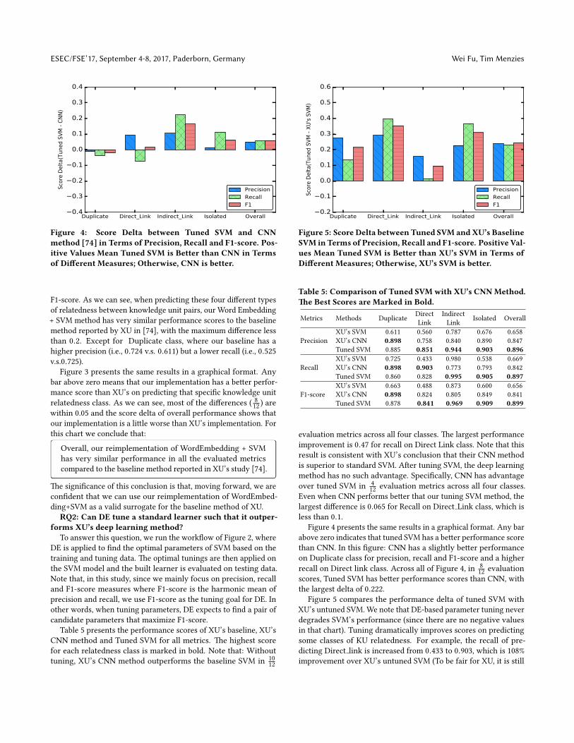
Figure 4: Score Delta between Tuned SVM and CNNmethod [74] in Terms of Precision, Recall and F1-score. Pos-itive Values Mean Tuned SVM is Better than CNN in Termsof Di�erent Measures; Otherwise, CNN is better.

F1-score. As we can see, when predicting these four di�erent typesof relatedness between knowledge unit pairs, our Word Embedding+ SVM method has very similar performance scores to the baselinemethod reported by XU in [74], with the maximum di�erence lessthan 0.2. Except for Duplicate class, where our baseline has ahigher precision (i.e., 0.724 v.s. 0.611) but a lower recall (i.e., 0.525v.s.0.725).

Figure 3 presents the same results in a graphical format. Anybar above zero means that our implementation has a be�er perfor-mance score than XU’s on predicting that speci�c knowledge unitrelatedness class. As we can see, most of the di�erences ( 8

12 ) arewithin 0.05 and the score delta of overall performance shows thatour implementation is a li�le worse than XU’s implementation. Forthis chart we conclude that:

Overall, our reimplementation of WordEmbedding + SVMhas very similar performance in all the evaluated metricscompared to the baseline method reported in XU’s study [74].

�e signi�cance of this conclusion is that, moving forward, we arecon�dent that we can use our reimplementation of WordEmbed-ding+SVM as a valid surrogate for the baseline method of XU.

RQ2: Can DE tune a standard learner such that it outper-forms XU’s deep learning method?

To answer this question, we run the work�ow of Figure 2, whereDE is applied to �nd the optimal parameters of SVM based on thetraining and tuning data. �e optimal tunings are then applied onthe SVM model and the built learner is evaluated on testing data.Note that, in this study, since we mainly focus on precision, recalland F1-score measures where F1-score is the harmonic mean ofprecision and recall, we use F1-score as the tuning goal for DE. Inother words, when tuning parameters, DE expects to �nd a pair ofcandidate parameters that maximize F1-score.

Table 5 presents the performance scores of XU’s baseline, XU’sCNN method and Tuned SVM for all metrics. �e highest scorefor each relatedness class is marked in bold. Note that: Withouttuning, XU’s CNN method outperforms the baseline SVM in 10

12

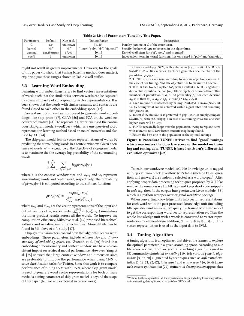
Figure 5: Score Delta between Tuned SVM and XU’s BaselineSVM inTerms of Precision, Recall and F1-score. Positive Val-ues Mean Tuned SVM is Better than XU’s SVM in Terms ofDi�erent Measures; Otherwise, XU’s SVM is better.

Table 5: Comparison of Tuned SVMwith XU’s CNNMethod.�e Best Scores are Marked in Bold.

Metrics Methods Duplicate DirectLink

IndirectLink Isolated Overall

PrecisionXU’s SVM 0.611 0.560 0.787 0.676 0.658XU’s CNN 0.898 0.758 0.840 0.890 0.847Tuned SVM 0.885 0.851 0.944 0.903 0.896

RecallXU’s SVM 0.725 0.433 0.980 0.538 0.669XU’s CNN 0.898 0.903 0.773 0.793 0.842Tuned SVM 0.860 0.828 0.995 0.905 0.897

F1-scoreXU’s SVM 0.663 0.488 0.873 0.600 0.656XU’s CNN 0.898 0.824 0.805 0.849 0.841Tuned SVM 0.878 0.841 0.969 0.909 0.899

evaluation metrics across all four classes. �e largest performanceimprovement is 0.47 for recall on Direct Link class. Note that thisresult is consistent with XU’s conclusion that their CNN methodis superior to standard SVM. A�er tuning SVM, the deep learningmethod has no such advantage. Speci�cally, CNN has advantageover tuned SVM in 4

12 evaluation metrics across all four classes.Even when CNN performs be�er that our tuning SVM method, thelargest di�erence is 0.065 for Recall on Direct Link class, which isless than 0.1.

Figure 4 presents the same results in a graphical format. Any barabove zero indicates that tuned SVM has a be�er performance scorethan CNN. In this �gure: CNN has a slightly be�er performanceon Duplicate class for precision, recall and F1-score and a higherrecall on Direct link class. Across all of Figure 4, in 8

12 evaluationscores, Tuned SVM has be�er performance scores than CNN, withthe largest delta of 0.222.

Figure 5 compares the performance delta of tuned SVM withXU’s untuned SVM. We note that DE-based parameter tuning neverdegrades SVM’s performance (since there are no negative valuesin that chart). Tuning dramatically improves scores on predictingsome classes of KU relatedness. For example, the recall of pre-dicting Direct link is increased from 0.433 to 0.903, which is 108%improvement over XU’s untuned SVM (To be fair for XU, it is still


Figure 6: Score Delta between Tuned SVM and Our UntunedSVM inTerms of Precision, Recall and F1-score. Positive Val-ues Mean Tuned SVM is Better than Our Untuned SVM inTerms of Di�erent Measures; Otherwise, Our SVM is Better.

84% improvement over our untuned SVM). At the same time, thecorresponding precision and F1 scores of predicting Direct Linkare increased from 0.560 to 0.851 and 0.488 to 0.841, which are 52%and 72% improvement over XU’s original report[74], respectively.A similar pa�ern can also be observed in Isolated class. On average,tuning helps improve the performance of XU’s SVM by 0.238, 0.228and 0.227 in terms of precision, recall and F1-score for all four KUrelatedness classes. Figure 6 compares the tuned SVM with our un-tuned SVM. We note that we get the similar pa�erns that observedin Figure 5. All the bars are above zero, etc.

Based on the performance scores in Table 5 and score delta inFigure 4, Figure 5 and Figure 6, we can see that:

• Parameter tuning can dramatically improve the performance ofWord Embedding + SVM (the baseline method) for the multi-class KU relatedness prediction task;

• With the optimal tunings, the traditional machine learningmethod, SVM, if not be�er, is at least comparable with deeplearning methods (CNN).

When discussing this result with colleagues, we are sometimesasked for a statistical analysis that con�rms the above �nding.However, due the lack of evaluation score distributions of the CNNmethod in [74], we cannot compare their single value with ourresults from 10 repeated runs. However, according to Wilcoxonsinged rank test over 10 runs results, tuned SVM performs sta-tistically be�er than our untuned SVM in terms of all evaluationmeasures on all four classes (p < 0.05). According to Cli� δ values,the magnitude of di�erence between tuned SVM and our untunedSVM is not trivial (|δ | > 0.147) for all evaluation measures.

Overall, the experimental results and our analysis indicate that:

In the evaluation conducted here, the deep learning method,CNN, does not have any performance advantage over ourtuning approach.

RQ3: Is tuning SVM with DE faster than XU’s deep learn-ing method?

When comparing the runtime of two learning methods, it obvi-ously should be conducted under the same hardware se�ings. Sincewe adopt the CNN evaluation scores from [74], we can not run onour tuning SVM experiment under the exactly same system set-tings. To allow readers to have a objective comparison, we providethe experimental environment as shown in Table 6. To obtain theruntime of tuning SVM, we recorded the start time and end time ofthe program execution, including parameter tuning, training modeland testing model.

Table 6: Comparison of Experimental EnvironmentMethods OS CPU RAMTuning SVM MacOS 10.12 Intel Core i5 2.7 GHz 8 GBCNN Windows 7 Intel Core i7 2.5 GHz 16 GB

According to XU, it took 14 hours to train their CNN model intoa low loss convergence (< e−3) [74]. Our work, on the other handonly takes 10 minutes to run SVM with parameter tuning by DEon a similar environment. �at is, the simple parameter tuningmethod on SVM is 84X faster than XU’s deep learning method.

Compared to CNN method, tuning SVM is about 84X fasterin terms of model building.

�e signi�cance of this �nding is that, in this case study, CNNwas neither be�er in performance scores (see RQ2) nor runtimes.CNN’s extra runtimes are a particular concern since (a) they arevery long; and (b) these would be incurred anytime researcherswants to update the CNN model with new data or wanted to validatethe XU result.

6 DISCUSSION6.1 Why DE+SVM works?Parameter tuning matters. As mentioned in Section 2.4, the de-fault parameter values set by the algorithm designers could generatea good performance on average but may not guarantee the bestperformance for the local data [9, 21]. Given that, it is most strangeto report that most SE researchers ignore the impacts of parame-ter tuning when they utilize various machine learning methods toconduct so�ware analytic (evidence: see our reviews in [1, 21, 22]).�e conclusion of this work must be to stress the importance of thiskind of tuning, using local data, for any future so�ware analyticsstudy.

Better explore the searching space. It turns out that oneexception to our statement that “most researchers do not tune” isthe XU study. In that work, they unsuccessfully perform parametertuning, but with with grid search. In such a grid search, for Nparameters to be tuned, N for loops are created to run over a rangeof se�ings for each parameter. While a widely used method, itis o�en deprecated. For example, Bergstra et al.[9] note that gridsearch jumps through di�erent parameter se�ings between somemin and max values of pre-de�ned tuning range. �ey warn thatsuch jumps may actually skip over the critical tuning values. Onthe other hand, DE tuning values are adjusted based on be�ercandidates from previous generations. Hence DE is more likelythan grid search to “�ll in the gaps” between the initialized values.


�at said, although DE +SVM works in this study, it does notmean DE is the best parameter tuner for all SE tasks. We encouragemore researchers to explore faster and more e�ective parametertuners in this direction.

6.2 ImplicationBeyond the speci�cs of this case study, what general principles canwe take from the above work?

Understand the task. One reason to try di�erent tools for thesame task is to be�er understand the task. �e more we understanda task, the be�er we can match tools to that task. Tools that arepoorly matched to task are usually complex and/or slow to execute.In the case study of this paper, we would say that• Deep learning is a poor match to the task of predicting whether

two questions posted on Stack Over�ow are semantically link-able since it is so slow;

• Di�erential evolution tuning SVM is a much be�er match sinceit is so fast and obtain competitive performance.

�at said, it is important to stress that the point of this study isnot to deprecate deep learning. �ere are many scenarios werewe believe deep learning would be a natural choice (e.g. whenanalyzing complex speech or visual data). In SE, it is still an openresearch question that in which scenario deep learning is the bestchoice. Results from this paper show that, at least for classi�cationtasks like knowledge unit relatedness classi�cation on Stack Over-�ow, deep learning does not have much advantage over well tunedconventional machine learning methods. However, as we be�erunderstand SE tasks, deep learning could be used to address moreSE problems, which require more advanced arti�cial intelligence.

Treat resource constraints as design challenges. As a gen-eral engineering principle, we think it insightful to consider theresource cost of a tool before applying it. It turns out that thisis a design pa�ern used in contemporary industry. According toCalero and Pa�ini [11], many current commercial redesigns aremotivated (at least in part) by arguments based on sustainability(i.e. using fewer resources to achieve results). In fact, they say thatmanagers used sustainability-based redesigns to motivate extensivecost-cu�ing opportunities.

6.3 �reads to Validity�reats to internal validity concern the consistency of the resultsobtained from the result. In our study, to investigate how tuningcan improve the performance of baseline methods and how wellit perform compared with deep learning method. We select XU’sWord Embedding + SVM baseline method as a case study. Sincethe original implementation of Word Embedding + SVM (baseline2 method in [74]) is not publicly available, we have to reimplementour version of Word Embedding + SVM as the baseline methodin this study. As shown in RQ1, our implementation has quitesimilar results to XU’s on the same data sets. Hence, we believethat our implementation re�ect the original baseline method inXu’s study [74].

�reats to external validity represent if the results are of rele-vance for other cases, or the ability to generalize the observations ina study. In this study, we compare our tuning baseline method withdeep learning method, CNN, in terms of precision, recall, F1-score

and accuracy. �e experimental results are quite consistent forthis knowledge units relatedness prediction task. Nonetheless, wedo not claim that our �ndings can be generalized to all so�wareanalytics tasks. However, those other so�ware analytics tasks o�enapply deep learning methods on classi�cation tasks [15, 68] and soit is quite possible that the methods of this paper (i.e., DE-basedparameter tuning) would be widely applicable, elsewhere.

7 CONCLUSIONIn this paper, we perform a comparative study to investigate howtuning can improve the baseline method compared with state-of-the-art deep learning method for predicting knowledge units relat-edness on Stack Over�ow. Our experimental results show that:

• Tuning improves the performance of baseline methods. At leastfor Word Embedding + SVM (baseline in [74]) method, if notbe�er, it performs as well as the proposed CNN method in [74].

• �e baseline method with parameter tuning runs much fasterthan complicated deep learning. In this study, tuning SVM runs84X faster than CNN method.

8 ADDENDUMAs this paper was going to going to press we learned of a newdeep learning methods that, according to its creators, runs 20 timesfaster than standard deep learning [61]. Note that in that paper, theauthors say their faster method does not produce be�er results– infact, their method generated solutions that were a small fractionworse than “classic” deep learning. Hence, that paper does notinvalidate our result since (a) our DE-based method sometimesproduced be�er results than classic deep learning and (b) our DEruns 84 times faster (i.e. much faster runtimes than those reportedin [61]).

�at said, this new fast deep learner deserves our close a�entionsince, using it, we conjecture that our DE tools could solve an openproblem in the deep learning community; i.e. how to �nd the bestcon�gurations inside a deep learner faster.

Based on the results of this study, we recommend that beforeapplying deep learning method on SE tasks, implement simplertechniques. �ese simpler methods could be used, at the very least,for comparisons against a baseline. In this particular case of deeplearning vs DE, the extra computational e�ort is so very minor (10minutes on top of 14 hours), that such a “try-with-simpler” shouldbe standard practice.

As to the future work, we will explore more simple techniquesto solve SE tasks and also investigate how deep learning techniquescould be applied e�ectively in so�ware engineering �eld.

ACKNOWLEDGEMENTS�e work is partially funded by an NSF award #1302169.

REFERENCES[1] Amritanshu Agrawal, Wei Fu, and Tim Menzies. 2016. What is wrong with

topic modeling?(and how to �x it using search-based se). arXiv preprintarXiv:1608.08176 (2016).

[2] John Anvik, Lyndon Hiew, and Gail C Murphy. 2006. Who should �x this bug?.In Proceedings of the 28th International Conference on So�ware Engineering. ACM,361–370.


[3] Andrea Arcuri and Gordon Fraser. 2011. On parameter tuning in search basedso�ware engineering. In International Symposium on Search Based So�wareEngineering. Springer, 33–47.

[4] Itamar Arel, Derek C Rose, and �omas P Karnowski. 2010. Research Frontier:Deep Machine Learning–a New Frontier in Arti�cial Intelligence Research. IEEEComputational Intelligence Magazine 5, 4 (2010), 13–18.

[5] Anton Barua, Stephen W �omas, and Ahmed E Hassan. 2014. What are devel-opers talking about? an analysis of topics and trends in stack over�ow. EmpiricalSo�ware Engineering 19, 3 (2014), 619–654.

[6] Ricardo P Beausoleil. 2006. “MOSS” multiobjective sca�er search applied to non-linear multiple criteria optimization. European Journal of Operational Research169, 2 (2006), 426–449.

[7] Andrew Begel and �omas Zimmermann. 2014. Analyze this! 145 questions fordata scientists in so�ware engineering. In Proceedings of the 36th InternationalConference on So�ware Engineering. ACM, 12–23.

[8] Yoav Benjamini and Yosef Hochberg. 1995. Controlling the false discovery rate: apractical and powerful approach to multiple testing. Journal of the royal statisticalsociety. Series B (Methodological) (1995), 289–300.

[9] James Bergstra and Yoshua Bengio. 2012. Random search for hyper-parameteroptimization. Journal of Machine Learning Research 13, Feb (2012), 281–305.

[10] David Binkley, Daniel Heinz, Dawn Lawrie, and Justin Overfelt. 2014. Under-standing LDA in source code analysis. In Proceedings of the 22nd InternationalConference on Program Comprehension. ACM, 26–36.

[11] Coral Calero and Mario Pia�ini. 2015. Green in So�ware Engineering. (2015).[12] Jose M Chaves-Gonzalez and Miguel A Perez-Toledano. 2015. Di�erential evolu-

tion with Pareto tournament for the multi-objective next release problem. Appl.Math. Comput. 252 (2015), 1–13.

[13] Shyam R Chidamber and Chris F Kemerer. 1994. A metrics suite for objectoriented design. IEEE Transactions on So�ware Engineering 20, 6 (1994), 476–493.

[14] Ibtissem Chiha, J Ghabi, and Noureddine Liouane. 2012. Tuning PID controllerwith multi-objective di�erential evolution. In 2012 5th International Symposiumon Communications, Control and Signal Processing. IEEE, 1–4.

[15] Morakot Choetkiertikul, Hoa Khanh Dam, Truyen Tran, Trang Pham, AdityaGhose, and Tim Menzies. 2016. A deep learning model for estimating storypoints. arXiv preprint arXiv:1609.00489 (2016).

[16] Anna Corazza, Sergio Di Martino, Filomena Ferrucci, Carmine Gravino, FedericaSarro, and Emilia Mendes. 2013. Using tabu search to con�gure support vectorregression for e�ort estimation. Empirical So�ware Engineering 18, 3 (2013),506–546.

[17] Jacek Czerwonka, Rajiv Das, Nachiappan Nagappan, Alex Tarvo, and AlexTeterev. 2011. Crane: Failure prediction, change analysis and test prioritization inpractice–experiences from windows. In Proceedings of the 4th IEEE InternationalConference on So�ware Testing, Veri�cation and Validation. IEEE, 357–366.

[18] Karim O Elish and Mahmoud O Elish. 2008. Predicting defect-prone so�waremodules using support vector machines. Journal of Systems and So�ware 81, 5(2008), 649–660.

[19] Martin S Feather and Tim Menzies. 2002. Converging on the optimal a�ainmentof requirements. In Proceedings of the 10th Anniversary IEEE Joint InternationalConference on Requirements Engineering. IEEE, 263–270.

[20] Danyel Fisher, Rob DeLine, Mary Czerwinski, and Steven Drucker. 2012. Interac-tions with big data analytics. interactions 19, 3 (2012), 50–59.

[21] Wei Fu, Tim Menzies, and Xipeng Shen. 2016. Tuning for so�ware analytics: Isit really necessary? Information and So�ware Technology 76 (2016), 135–146.

[22] Wei Fu, Vivek Nair, and Tim Menzies. 2016. Why is di�erential evolution be�erthan grid search for tuning defect predictors? arXiv preprint arXiv:1609.02613(2016).

[23] Alex Graves, Abdel-rahman Mohamed, and Geo�rey Hinton. 2013. Speechrecognition with deep recurrent neural networks. In 2013 IEEE InternationalConference on Acoustics, Speech and Signal Processing. IEEE, 6645–6649.

[24] Xiaodong Gu, Hongyu Zhang, Dongmei Zhang, and Sunghun Kim. 2016. DeepAPI learning. In Proceedings of the 2016 24th ACM SIGSOFT International Sympo-sium on Foundations of So�ware Engineering. ACM, 631–642.

[25] Mark A Hall and Geo�rey Holmes. 2003. Benchmarking a�ribute selectiontechniques for discrete class data mining. IEEE Transactions on Knowledge andData engineering 15, 6 (2003), 1437–1447.

[26] Maurice Howard Halstead. 1977. Elements of so�ware science. Vol. 7. ElsevierNew York.

[27] Mark Harman. 2007. �e current state and future of search based so�wareengineering. In 2007 Future of So�ware Engineering. IEEE Computer Society,342–357.

[28] Tian Jiang, Lin Tan, and Sunghun Kim. 2013. Personalized defect prediction. InProceedings of the 28th IEEE/ACM International Conference on Automated So�wareEngineering. IEEE, 279–289.

[29] �orsten Joachims. 1998. Text categorization with support vector machines:Learning with many relevant features. In European Conference on Machine Learn-ing. Springer, 137–142.

[30] Bryan F Jones, H-H Sthamer, and David E Eyres. 1996. Automatic structuraltesting using genetic algorithms. So�ware Engineering Journal 11, 5 (1996),

299–306.[31] Dennis Kafura and Geereddy R. Reddy. 1987. �e use of so�ware complexity

metrics in so�ware maintenance. IEEE Transactions on So�ware Engineering 3(1987), 335–343.

[32] Dongsun Kim, Yida Tao, Sunghun Kim, and Andreas Zeller. 2013. Where shouldwe �x this bug? a two-phase recommendation model. IEEE Transactions onSo�ware Engineering 39, 11 (2013), 1597–1610.

[33] Sunghun Kim, E James Whitehead Jr, and Yi Zhang. 2008. Classifying so�warechanges: Clean or buggy? IEEE Transactions on So�ware Engineering 34, 2 (2008),181–196.

[34] Ekrem Kocaguneli, Tim Menzies, Ayse Bener, and Jacky W Keung. 2012. Ex-ploiting the essential assumptions of analogy-based e�ort estimation. IEEETransactions on So�ware Engineering 38, 2 (2012), 425–438.

[35] Ekrem Kocaguneli, Tim Menzies, and Jacky W Keung. 2012. On the value ofensemble e�ort estimation. IEEE Transactions on So�ware Engineering 38, 6(2012), 1403–1416.

[36] Joseph Krall, Tim Menzies, and Misty Davies. 2015. Gale: Geometric activelearning for search-based so�ware engineering. IEEE Transactions on So�wareEngineering 41, 10 (2015), 1001–1018.

[37] Alex Krizhevsky, Ilya Sutskever, and Geo�rey E Hinton. 2012. Imagenet classi�ca-tion with deep convolutional neural networks. In Advances in Neural InformationProcessing Systems. 1097–1105.

[38] Rakesh Kumar, Keith I Farkas, Norman P Jouppi, Parthasarathy Ranganathan,and Dean M Tullsen. 2003. Single-ISA heterogeneous multi-core architectures:�e potential for processor power reduction. In Proceedings of the 36th AnnualIEEE/ACM International Symposium on Microarchitecture. IEEE, 81–92.

[39] An Ngoc Lam, Anh Tuan Nguyen, Hoan Anh Nguyen, and Tien N Nguyen. 2015.Combining deep learning with information retrieval to localize buggy �les forbug reports (n). In Proceedings of the 2015 30th IEEE/ACM International Conferenceon Automated So�ware Engineering. IEEE, 476–481.

[40] �oc V Le. 2013. Building high-level features using large scale unsupervisedlearning. In 2013 IEEE International Conference on Acoustics, Speech and SignalProcessing. IEEE, 8595–8598.

[41] Remi Lebret and Ronan Collobert. 2013. Word emdeddings through hellingerPCA. arXiv preprint arXiv:1312.5542 (2013).

[42] Yann LeCun, Yoshua Bengio, and Geo�rey Hinton. 2015. Deep learning. Nature521, 7553 (2015), 436–444.

[43] Stefan Lessmann, Bart Baesens, Christophe Mues, and Swantje Pietsch. 2008.Benchmarking classi�cation models for so�ware defect prediction: A proposedframework and novel �ndings. IEEE Transactions on So�ware Engineering 34, 4(2008), 485–496.

[44] Lisha Li, Kevin Jamieson, Giulia DeSalvo, Afshin Rostamizadeh, and AmeetTalwalkar. 2016. Hyperband: a novel bandit-based approach to hyperparameteroptimization. arXiv preprint arXiv:1603.06560 (2016).

[45] �omas J McCabe. 1976. A complexity measure. IEEE Transactions on So�wareEngineering 4 (1976), 308–320.

[46] Tim Menzies, Jeremy Greenwald, and Art Frank. 2007. Data mining static codea�ributes to learn defect predictors. IEEE Transactions on So�ware Engineering33, 1 (2007).

[47] Tomas Mikolov, Ilya Sutskever, Kai Chen, Greg S Corrado, and Je� Dean. 2013.Distributed representations of words and phrases and their compositionality. InAdvances in Neural Information Processing Systems. 3111–3119.

[48] Mohamed Wiem Mkaouer, Marouane Kessentini, Slim Bechikh, Kalyanmoy Deb,and Mel O Cinneide. 2014. High dimensional search-based so�ware engineer-ing: �nding tradeo�s among 15 objectives for automating so�ware refactoringusing NSGA-III. In Proceedings of the 2014 Annual Conference on Genetic andEvolutionary Computation. ACM, 1263–1270.

[49] Julian Molina, Manuel Laguna, Rafael Martı, and Rafael Caballero. 2007. SSPMO:A sca�er tabu search procedure for non-linear multiobjective optimization. IN-FORMS Journal on Computing 19, 1 (2007), 91–100.

[50] Kjetil Molokken and Magen Jorgensen. 2003. A review of so�ware surveys onso�ware e�ort estimation. In Proceedings of the 2003 International Symposium onEmpirical So�ware Engineering. IEEE, 223–230.

[51] Gordon E Moore and others. 1998. Cramming more components onto integratedcircuits. Proc. IEEE 86, 1 (1998), 82–85.

[52] Lili Mou, Ge Li, Lu Zhang, Tao Wang, and Zhi Jin. 2016. Convolutional NeuralNetworks over Tree Structures for Programming Language Processing. In Pro-ceedings of the �irtieth AAAI Conference on Arti�cial Intelligence. AAAI Press,1287–1293.

[53] Mahamed GH Omran, Andries Petrus Engelbrecht, and Ayed Salman. 2005.Di�erential evolution methods for unsupervised image classi�cation. In 2005IEEE Congress on Evolutionary Computation, Vol. 2. IEEE, 966–973.

[54] �omas J Ostrand, Elaine J Weyuker, and Robert M Bell. 2004. Where the bugsare. In ACM SIGSOFT So�ware Engineering Notes, Vol. 29. ACM, 86–96.

[55] Fabian Pedregosa, Gael Varoquaux, Alexandre Gramfort, Vincent Michel,Bertrand �irion, Olivier Grisel, Mathieu Blondel, Peter Pre�enhofer, Ron Weiss,Vincent Dubourg, and others. 2011. Scikit-learn: machine learning in Python.Journal of Machine Learning Research 12, Oct (2011), 2825–2830.


[56] Je�rey Pennington, Richard Socher, and Christopher D Manning. 2014. Glove:global vectors for word representation. In EMNLP, Vol. 14. 1532–1543.

[57] Mukund Raghothaman, Yi Wei, and Youssef Hamadi. 2016. SWIM: synthesizingwhat I mean: code search and idiomatic snippet synthesis. In Proceedings of the38th International Conference on So�ware Engineering. ACM, 357–367.

[58] Radim Rehurek and Petr Sojka. 2010. So�ware framework for topic modellingwith large corpora. In In Proceedings of the LREC 2010Workshop on NewChallengesfor NLP Frameworks. Citeseer.

[59] Jeanine Romano, Je�rey D Kromrey, Jesse Coraggio, Je� Skowronek, and LindaDevine. 2006. Exploring methods for evaluating group di�erences on the NSSEand other surveys: Are the t-test and Cohen�sd indices the most appropriatechoices. In Annual Meeting of the Southern Association for Institutional Research.

[60] Jurgen Schmidhuber. 2015. Deep learning in neural networks: An overview.Neural networks 61 (2015), 85–117.

[61] Ryan Spring and Anshumali Shrivastava. 2017. Scalable and sustainable deeplearning via randomized hashing. In Proceedings of the 23rd ACM SIGKDD Inter-national Conference on Knowledge Discovery and Data Mining. ACM.

[62] R. Storn and K. Price. 1997. Di�erential evolution–a simple and e�cient heuristicfor global optimization over continuous spaces. Journal of global optimization11, 4 (1997), 341–359.

[63] Ilya Sutskever, Oriol Vinyals, and �oc V Le. 2014. Sequence to sequencelearning with neural networks. In Advances in Neural Information ProcessingSystems. 3104–3112.

[64] Chakkrit Tantithamthavorn, Shane McIntosh, Ahmed E Hassan, and KenichiMatsumoto. 2016. Automated parameter optimization of classi�cation techniquesfor defect prediction models. In Proceedings of the 38th International Conferenceon So�ware Engineering. ACM, 321–332.

[65] Christopher �eisen, Kim Herzig, Patrick Morrison, Brendan Murphy, and LaurieWilliams. 2015. Approximating a�ack surfaces with stack traces. In Proceedingsof the 37th International Conference on So�ware Engineering-Volume 2. IEEE,199–208.

[66] Jakob Vesterstrom and Rene �omsen. 2004. A comparative study of di�erentialevolution, particle swarm optimization, and evolutionary algorithms on numer-ical benchmark problems. In Proceedings of the 2004 Congress on EvolutionaryComputation, Vol. 2. IEEE, 1980–1987.

[67] Jue Wang, Yingnong Dang, Hongyu Zhang, Kai Chen, Tao Xie, and DongmeiZhang. 2013. Mining succinct and high-coverage API usage pa�erns fromsource code. In Proceedings of the 10th Working Conference on Mining So�wareRepositories. IEEE, 319–328.

[68] Song Wang, Taiyue Liu, and Lin Tan. 2016. Automatically learning semanticfeatures for defect prediction. In Proceedings of the 38th International Conferenceon So�ware Engineering. ACM, 297–308.

[69] Tiantian Wang, Mark Harman, Yue Jia, and Jens Krinke. 2013. Searching forbe�er con�gurations: a rigorous approach to clone evaluation. In Proceedings ofthe 2013 9th Joint Meeting on Foundations of So�ware Engineering. ACM, 455–465.

[70] Martin White, Michele Tufano, Christopher Vendome, and Denys Poshyvanyk.2016. Deep learning code fragments for code clone detection. In Proceedings ofthe 31st IEEE/ACM International Conference on Automated So�ware Engineering.ACM, 87–98.

[71] Martin White, Christopher Vendome, Mario Linares-Vasquez, and Denys Poshy-vanyk. 2015. Toward deep learning so�ware repositories. In Proceedings of the12th Working Conference on Mining So�ware Repositories. IEEE, 334–345.

[72] Andreas Windisch, Stefan Wappler, and Joachim Wegener. 2007. Applyingparticle swarm optimization to so�ware testing. In Proceedings of the 9th AnnualConference on Genetic and Evolutionary Computation. ACM, 1121–1128.

[73] David H Wolpert. 1996. �e lack of a priori distinctions between learningalgorithms. Neural computation 8, 7 (1996), 1341–1390.

[74] Bowen Xu, Deheng Ye, Zhenchang Xing, Xin Xia, Guibin Chen, and Shanping Li.2016. Predicting semantically linkable knowledge in developer online forums viaconvolutional neural network. In Proceedings of the 31st IEEE/ACM InternationalConference on Automated So�ware Engineering. ACM, 51–62.

[75] Xiao Yang, Craig Macdonald, and Iadh Ounis. 2016. Using word embeddings intwi�er election classi�cation. arXiv preprint arXiv:1606.07006 (2016).

[76] Xin Ye, Razvan Bunescu, and Chang Liu. 2014. Learning to rank relevant �les forbug reports using domain knowledge. In Proceedings of the 22nd ACM SIGSOFTInternational Symposium on Foundations of So�ware Engineering. ACM, 689–699.

[77] Zhenlong Yuan, Yongqiang Lu, Zhaoguo Wang, and Yibo Xue. 2014. Droid-sec: deep learning in android malware detection. In ACM SIGCOMM ComputerCommunication Review, Vol. 44. ACM, 371–372.

[78] Yuanyuan Zhang, Mark Harman, and S. Afshin Mansouri. 2007. �e multi-objective next release problem. In Proceedings of the 9th Annual Conference onGenetic and Evolutionary Computation. 1129–1137.

[79] Jian Zhou, Hongyu Zhang, and David Lo. 2012. Where should the bugs be �xed?-more accurate information retrieval-based bug localization based on bug reports.In Proceedings of the 34th International Conference on So�ware Engineering. IEEE,14–24.

[80] Guido Zuccon, Bevan Koopman, Peter Bruza, and Leif Azzopardi. 2015. Inte-grating and evaluating neural word embeddings in information retrieval. InProceedings of the 20th Australasian Document Computing Symposium. ACM, 12.

Documents

Easy over Hard: A Case Study on Deep Learning over Hard: A Case Study on Deep Learning ESEC/FSE’17, September 4-8, 2017, Paderborn, Germany