Embed Size (px)
Citation preview

LETTERSPUBLISHED ONLINE: 9 MAY 2016 | DOI: 10.1038/NGEO2713
Earth’s air pressure 2.7 billion years agoconstrained to less than half of modern levelsSanjoy M. Som1*†, Roger Buick1, JamesW. Hagadorn2, Tim S. Blake3, John M. Perreault1†,Jelte P. Harnmeijer1† and David C. Catling1
How the Earth stayed warm several billion years ago whenthe Sun was considerably fainter is the long-standing problemof the ‘faint young Sun paradox’. Because of negligible1 O2and only moderate CO2 levels2 in the Archaean atmosphere,methane has been invoked as an auxiliary greenhouse gas3.Alternatively, pressure broadening in a thicker atmospherewith a N2 partial pressure around 1.6–2.4 bar could haveenhanced the greenhouse e�ect4. But fossilized raindropimprints indicate that air pressure 2.7 billion years ago(Gyr) was below twice modern levels and probably below1.1 bar, precluding such pressure enhancement5. This resultis supported by nitrogen and argon isotope studies of fluidinclusions in 3.0–3.5Gyr rocks6. Here, we calculate absoluteArchaean barometric pressure using the size distributionof gas bubbles in basaltic lava flows that solidified at sealevel ∼2.7Gyr in the Pilbara Craton, Australia. Our dataindicate a surprisingly low surface atmospheric pressureof Patm=0.23±0.23 (2σ ) bar, and combined with previousstudies suggests ∼0.5 bar as an upper limit to late ArchaeanPatm. The result implies that the thin atmosphere was richin auxiliary greenhouse gases and that Patm fluctuated overgeologic time to a previously unrecognized extent.
Air pressure constrains atmospheric composition and climate,in turn influencing biological evolution. However, it has provedvery difficult to measure atmospheric pressure over geologic timebecause such a barely perceptible property has minimal impacton most rocks. Nevertheless, Archaean air pressure has beenconstrained by independent methods5,6 to ≤1.2 bar. Here, we moretightly constrain ancient air pressure by applying a new proxy tothe Archaean eon: the size distribution of gas bubbles (vesicles) inbasaltic lava flows erupted at sea level.
The principle involved in using vesicles in basaltic lava flows forpalaeobarometry is that the average vesicle size at the very top ofa flow is constrained by atmospheric pressure alone, whereas theaverage vesicle size at the flow base is controlled by the weightof the lava above added to the atmospheric pressure7. Thus, thedifference in size between large vesicles at the flow top and smallervesicles at the flow base allows atmospheric pressure to be deducedonce basalt density and flow thickness are known. This differentialtechnique is independent of absolute volatile content in the lava,and has been verified as a geologic altimeter on modern flows inHawaii, where elevations are known8. It has also been used to inferthe uplift rate of the Colorado plateau9, yielding results consistent
with thermochronology10, and has been applied to palaeoaltimetryin China11 and Turkey12. However, the technique can be usedonly on appropriate lava flows, which must be relatively thin, andhave cooled from top-down and bottom-up without inflation byinjection of newmolten material. In such flows, vesiculation mostlyaccumulates in upper (UVZ) and lower (LVZ) vesicular zones13.Furthermore, external gas recharge and deflation by drainage mustbe precluded. Bubbles trapped in the middle of a lava flow mayoriginate from new lava or gas injection, with inflation generallylimited to flows on slopes<2◦ (ref. 14).
The difference in size between the bubbles trapped in the UVZand LVZ is related to atmospheric pressure Patm (in Pa) by thecombined gas law:
PatmVUVZ
Tfreeze=(Patm+ρgH)VLVZ
Tfreeze⇒Patm=ρgH(Vr−1)−1 (1)
Here ρ is the lava density (typically 2,650 kgm−3 for basalt15), Tfreezethe temperature at which the lava solidifies at the flow top andbottom, g the gravitational acceleration (9.8m s−2),H the thicknessof the flow (m), and Vr the ratio VUVZ/VLVZ of the mean volume ofUVZ to LVZ bubbles8.
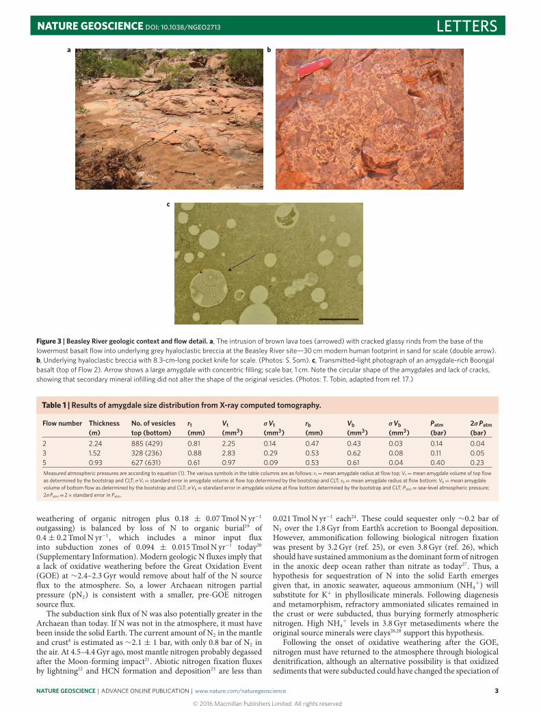
We examined gas bubbles in subaerial basaltic lava flows fromthe ∼2.74Gyr upper Boongal Formation to determine air pressureat that time. Thesemassive pahoehoe flowswith billowy scoriaceousflow tops occur in the Pilbara Craton of Western Australia wherethey are exposed along the Beasley River (Fig. 1). Five conformablesubaerial flows (numbered 1–5 in Fig. 2) immediately overliehyaloclastic breccias capping a thick pile of pillow basalts andhyaloclastites16. Two additional localities with similar hyaloclastite–pahoehoe transitions were also investigated (flows 6 and 7 in Fig. 1),one ∼12 km laterally along strike at Moona Well (flow 7) andthe other ∼1 km stratigraphically higher in the middle BunjinahFormation (flow 6). The intrusion of lava toes with crackedglassy rinds from the base of the lowermost basalt flow (Fig. 3a)into underlying hyaloclastic breccia (Fig. 3b) indicates terrestrialemplacement of a pahoehoe lava delta on unconsolidated wetbeach gravel. The lateral extent, over 300 km east–west, andthickness, ∼1 km, of the subaqueous basalt pile beneath the beachdeposits strongly suggest that the subaerial basalt flows wereemplaced beside an ocean at sea level (Supplementary Information).Field observations were used to identify flows that were simplyemplaced (minimally inflated or deflated without gas recharge) for
1Department of Earth and Space Sciences and Astrobiology Program, University of Washington, Seattle, Washington 98195, USA. 2Department of EarthSciences, Denver Museum of Nature & Science, Denver, Colorado 80205, USA. 3School of Earth and Environment, University of Western Australia,35 Stirling Highway, Crawley, Western Australia 6009, Australia. †Present addresses: Blue Marble Space Institute of Science, Seattle, Washington 98154,USA, and NASA Ames Research Center, Mo�ett Field, California 94035, USA (S.M.S.); Department of Geology and Geophysics, University ofAlaska—Fairbanks, Alaska 99775, USA (J.M.P.); James Hutton Institute, Invergowrie, Dundee DD2 5DA, UK (J.P.H.). *e-mail: [email protected]
NATURE GEOSCIENCE | ADVANCE ONLINE PUBLICATION | www.nature.com/naturegeoscience 1
© 2016 Macmillan Publishers Limited. All rights reserved

LETTERS NATURE GEOSCIENCE DOI: 10.1038/NGEO2713
Geologic boundary (exposed)
Geologic boundary (concealed)
Fault (exposed)
Fault (concealed)
Rocklea Dome
AFh
AFh
AFh
AFo
AFo
AFo
AFo
AFo
AFp
AFp
AFpAFpAFp
AFp
AFu
AFu
AFuAFu AFj
Hamersley Group
N
S
W E
br
brn
mwBeasley River
Sampling locality:brn: Beasley River Northbr: Beasley Rivermw: Moona Well
Fortescue Group
AFh: Hardey formationAFo: Boongal formationAFp: Pyradie formationAFu: Bunjinah formationAFj: Jeerinah formation
3 km
23° 50′ S117° 12′ E 117° 30′ E
23° 39′ S
AFj
AFj
Latit
ude
Longitude
Figure 1 | Geology of the Beasley River field area, southwestern Pilbara, and sampling localities. Flows 1–5 are at the Beasley River site (br), Flow 6 is atthe Beasley River North locality (brn), and Flow 7 was at Moona Well (mw).
T1B2
T3T5B4B3
T2
T4B5
Figure 2 | Beasley River locality (‘br’ in Fig. 1) with the locations of fiveconformable subaerial lava flows, along with the location of collectedsamples. T, flow top; B, flow bottom. Flow 1 did not have a basal exposure.Geologist (R.B.) in top-left box for scale. (Photos: S. Som.)
subsequent analysis (Supplementary Information). These selectioncriteria reduced the seven flows studied to only three suitable foranalysis: flows 2, 3 and 5 of the Boongal Formation at BeasleyRiver (Fig. 2).
Vesicles in lava flows preserve the original dimensions of the gasbubbles. The rocks underwent pre-compactional alteration duringwhich the vesicles were filled by the secondary minerals quartz,calcite and chlorite to form amygdales17. Infilling occurred bypassive precipitation without deformation, shown by the absenceof expansion or contraction cracks around the amygdales17 inthin section (Fig. 3c) and by their spherical shape in all but theuppermost flow crusts, where they are ellipsoidal owing to viscousstretching in the solidifying lava. Later low-grade metamorphism(sub-greenschist to lowermost greenschist facies) transformed thebasalt matrix to a chlorite–albite–epidote–actinolite assemblagewith little concomitant deformation; in the field the rocks areunfoliated and only openly folded with dips of less than 50◦. Thesepost-depositional effects altered neither the thickness of the flows
nor the size of the amygdales, shown by spherical rather than oblateor prolate shape of the amygdales.
Cores were drilled in samples collected from each UVZ andLVZ for subsequent X-ray analyses. Amygdales were identified bydensity contrast in the X-ray slices of the cores using a dynamicthresholding algorithm17. Tomography software BLOB3D18 stackedthe resulting binary images to determine amygdale dimensions.Mean amygdale volumes and their uncertainties were obtainedby bootstrap statistical resampling coupled with the Central LimitTheorem (CLT) (Methods and Supplementary Information). TheCLT states that the means of samples taken randomly from apopulation will be normally distributed, and the mean of thisdistribution will be the mean of the population. The standarddeviation in the bootstrap sampling distribution of the mean gaveerror bars for the amygdale volumes in the UVZ and LVZ.
In an uninflated flow of thickness H , the vesicle size differenceacross the flow records atmospheric pressure. Fromequation (1), theuncertainty in pressure results from combining the uncertainties inthe vesicle volumes in theUVZandLVZ, the flow thickness, and lavadensity (Supplementary Information). Results are shown in Table 1.The average pressure calculated from the three suitable flows sug-gests that the sea-level air pressure at 2.74Gyr was 0.23± 0.23 bar(2σ error—see Methods). The ‘most probable’ air-pressure upperlimit obtained from nearly contemporaneous 2.73Gyr fossil rain-drop impressions5 was 0.52–1.1 bar, whereas isotopic studies6 on3.0–3.5Gyr rocks suggest an upper limit of 0.5–1.2 bar. By combin-ing these previous results with this study, we obtain amore stringentupper limit on the air pressure at∼2.7Gyr of∼0.5 bar.
A balance of N source and sink fluxes that differs fromthe modern balance is needed to explain an unusually lowArchaean air pressure (much less than obtained by subtracting0.2 bar of the current O2 level). At present, a N source flux of0.33 ± 0.08 TmolN yr−1 (composed of 0.15 ± 0.03 TmolN yr−1
2
© 2016 Macmillan Publishers Limited. All rights reserved
NATURE GEOSCIENCE | ADVANCE ONLINE PUBLICATION | www.nature.com/naturegeoscience
NATURE GEOSCIENCE DOI: 10.1038/NGEO2713 LETTERSa b
c
Figure 3 | Beasley River geologic context and flow detail. a, The intrusion of brown lava toes (arrowed) with cracked glassy rinds from the base of thelowermost basalt flow into underlying grey hyaloclastic breccia at the Beasley River site—30 cm modern human footprint in sand for scale (double arrow).b, Underlying hyaloclastic breccia with 8.3-cm-long pocket knife for scale. (Photos: S. Som). c, Transmitted-light photograph of an amygdale-rich Boongalbasalt (top of Flow 2). Arrow shows a large amygdale with concentric filling; scale bar, 1 cm. Note the circular shape of the amygdales and lack of cracks,showing that secondary mineral infilling did not alter the shape of the original vesicles. (Photos: T. Tobin, adapted from ref. 17.)
Table 1 |Results of amygdale size distribution from X-ray computed tomography.
Flow number Thickness(m)
No. of vesiclestop (bottom)
rt(mm)
Vt(mm3)
σVt(mm3)
rb(mm)
Vb(mm3)
σVb(mm3)
Patm(bar)
2σPatm(bar)
2 2.24 885 (429) 0.81 2.25 0.14 0.47 0.43 0.03 0.14 0.043 1.52 328 (236) 0.88 2.83 0.29 0.53 0.62 0.08 0.11 0.055 0.93 627 (631) 0.61 0.97 0.09 0.53 0.61 0.04 0.40 0.23Measured atmospheric pressures are according to equation (1). The various symbols in the table columns are as follows: rt=mean amygdale radius at flow top; Vt=mean amygdale volume of top flowas determined by the bootstrap and CLT; σVt= standard error in amygdale volume at flow top determined by the bootstrap and CLT; rb=mean amygdale radius at flow bottom; Vb=mean amygdalevolume of bottom flow as determined by the bootstrap and CLT; σVb= standard error in amygdale volume at flow bottom determined by the bootstrap and CLT; Patm= sea-level atmospheric pressure;2σPatm=2×standard error in Patm .
weathering of organic nitrogen plus 0.18 ± 0.07 TmolN yr−1outgassing) is balanced by loss of N to organic burial19 of0.4± 0.2 TmolN yr−1, which includes a minor input fluxinto subduction zones of 0.094 ± 0.015 TmolN yr−1 today20(Supplementary Information). Modern geologic N fluxes imply thata lack of oxidative weathering before the Great Oxidation Event(GOE) at ∼2.4–2.3Gyr would remove about half of the N sourceflux to the atmosphere. So, a lower Archaean nitrogen partialpressure (pN2) is consistent with a smaller, pre-GOE nitrogensource flux.
The subduction sink flux of N was also potentially greater in theArchaean than today. If N was not in the atmosphere, it must havebeen inside the solid Earth. The current amount of N2 in the mantleand crust4 is estimated as ∼2.1 ± 1 bar, with only 0.8 bar of N2 inthe air. At 4.5–4.4Gyr ago, most mantle nitrogen probably degassedafter the Moon-forming impact21. Abiotic nitrogen fixation fluxesby lightning22 and HCN formation and deposition23 are less than
0.021 TmolN yr−1 each24. These could sequester only ∼0.2 bar ofN2 over the 1.8Gyr from Earth’s accretion to Boongal deposition.However, ammonification following biological nitrogen fixationwas present by 3.2Gyr (ref. 25), or even 3.8Gyr (ref. 26), whichshould have sustained ammonium as the dominant form of nitrogenin the anoxic deep ocean rather than nitrate as today27. Thus, ahypothesis for sequestration of N into the solid Earth emergesgiven that, in anoxic seawater, aqueous ammonium (NH4
+) willsubstitute for K+ in phyllosilicate minerals. Following diagenesisand metamorphism, refractory ammoniated silicates remained inthe crust or were subducted, thus burying formerly atmosphericnitrogen. High NH4
+ levels in 3.8Gyr metasediments where theoriginal source minerals were clays26,28 support this hypothesis.
Following the onset of oxidative weathering after the GOE,nitrogen must have returned to the atmosphere through biologicaldenitrification, although an alternative possibility is that oxidizedsediments that were subducted could have changed the speciation of
NATURE GEOSCIENCE | ADVANCE ONLINE PUBLICATION | www.nature.com/naturegeoscience
© 2016 Macmillan Publishers Limited. All rights reserved
3

LETTERS NATURE GEOSCIENCE DOI: 10.1038/NGEO2713
nitrogen in the mantle wedge29 from NH4+ to N2, allowing a greater
N2 flux from volcanic arcs. With the modern ∼0.33 TmolN yr−1released by volcanoes and weathering, 0.3 bar of N2 would bereplenished in∼0.33Gyr (Supplementary Information).
Low Archaean air pressure makes it difficult to reconcile the‘faint young Sun’ with the geologic record by invoking enhancedatmospheric infrared absorption4 caused by high pN2. Rather,greenhouse gases such as methane must have augmented thegreenhouse effect provided by moderate levels of CO2. If themean Patm (0.23 bar) indicated by our data represents the actualatmospheric pressure during the late Archaean, the correspondingboiling point of water at ∼58 ◦C would be an upper bound toambient temperature. Furthermore, results from photochemicalmodels of the Archaean atmosphere, such as those that explain therecord of mass-independent isotopic fractionation of sulfur, mightneed to be re-evaluated, because air pressure affects penetration ofultraviolet light and pressure-dependent photochemical reactions.Finally, the 0.5 bar upper limit to Archaean air pressure indicatedby our results implies that Patm has fluctuated over time toa greater extent than previously recognized, and that standardtemperature and pressure (STP) cannot be presumed for Archaeanchemical reactions.
MethodsMethods and any associated references are available in the onlineversion of the paper.
Received 8 March 2016; accepted 13 April 2016;published online 9 May 2016
References1. Holland, H. D. The oxygenation of the atmosphere and oceans. Phil. Trans. R.
Soc. B 361, 903–915 (2006).2. Sheldon, N. D. Precambrian paleosols and atmospheric CO2 levels. Precambr.
Res. 147, 148–155 (2006).3. Kasting, J. F. & Siefert, J. L. Life and the evolution of Earth’s atmosphere. Science
296, 1066–1068 (2002).4. Goldblatt, C. et al . Nitrogen-enhanced greenhouse warming on early Earth.
Nature Geosci. 2, 891–896 (2009).5. Som, S. M., Catling, D. C., Harnmeijer, J. P., Polivka, P. M. & Buick, R. Air
density 2.7 billion years ago limited to less than twice modern levels by fossilraindrop imprints. Nature 484, 359–362 (2012).
6. Marty, B., Zimmermann, L., Pujol, M., Burgess, R. & Philippot, P. Nitrogenisotopic composition and density of the Archean atmosphere. Science 342,101–104 (2013).
7. Sahagian, D. L. & Maus, J. E. Basalt vesicularity as a measure of atmosphericpressure and palaeoelevation. Nature 372, 449–451 (1994).
8. Sahagian, D., Proussevitch, A. & Carlson, W. Analysis of vesicular basalts andlava emplacement processes for application as apaleobarometer/paleoaltimeter. J. Geol. 110, 671–685 (2002).
9. Sahagian, D., Proussevitch, A. & Carlson, W. Timing of Colorado Plateau uplift:initial constraints from vesicular basalt-derived paleoelevations. Geology 30,807–810 (2002).
10. Flowers, R. & Farley, K. Apatite 4He/3He and (U-Th)/He evidence for anancient Grand Canyon. Science 338, 1616–1619 (2012).
11. Xia, G. Q., Yi, H. S., Zhao, X. X., Gong, D. X. & Ji, C. J. A late Mesozoic highplateau in eastern China: evidence from basalt vesicular paleoaltimetry. Chin.Sci. Bull. 57, 2767–2777 (2012).
12. Aydar, E. et al . Central Anatolian Plateau, Turkey: incision and paleoaltimetryrecorded from volcanic rocks. Turk. J. Earth Sci. 22, 739–746 (2013).
13. Aubele, J. C., Crumpler, L. & Elston, W. E. Vesicle zonation and verticalstructure of basalt flows. J. Volcanol. Geotherm. Res. 35, 349–374 (1988).
14. Hon, K., Kauahikaua, J., Denlinger, R. & Mackay, K. Emplacement andinflation of pahoehoe sheet flows: observations and measurements of activelava flows on Kilauea Volcano, Hawaii. Geol. Soc. Am. Bull. 106,351–370 (1994).
15. Moore, J. G. Density of basalt core from Hilo drill hole, Hawaii. J. Volcanol.Geotherm. Res. 112, 221–230 (2001).
16. Blake, T. S. Late Archaean crustal extension, sedimentary basin formation,flood basalt volcanism and continental rifting: the Nullagine and Mount JopeSupersequences, Western Australia. Precambr. Res. 60, 185–241 (1993).
17. Som, S. M. et al . Quantitative discrimination between geological materials withvariable density contrast by high resolution X-ray computed tomography:an example using amygdule size-distribution in ancient lava flows. Comput.Geosci. 54, 231–238 (2013).
18. Ketcham, R. A. Computational methods for quantitative analysis ofthree-dimensional features in geological specimens. Geosphere 1, 32–41 (2005).
19. Berner, R. Geological nitrogen cycle and atmospheric N2 over Phanerozoictime. Geology 34, 413–415 (2006).
20. Busigny, V., Cartigny, P. & Philippot, P. Nitrogen isotopes in ophioliticmetagabbros: a re-evaluation of modern nitrogen fluxes in subduction zonesand implication for the early Earth atmosphere. Geochim. Cosmochim. Acta 75,7502–7521 (2011).
21. Turner, G. The outgassing history of the Earth’s atmosphere. J. Geol. Soc. Lond.146, 147–154 (1989).
22. Navarro-González, R., McKay, C. P. & Mvondo, D. N. A possible nitrogen crisisfor Archaean life due to reduced nitrogen fixation by lightning. Nature 412,61–64 (2001).
23. Zahnle, K. J. Photochemistry of methane and the formation of hydrocyanic acid(HCN) in the Earth’s early atmosphere. J. Geophys. Res. 91, 2819–2834 (1986).
24. Kasting, J. F. & Siefert, J. L. The nitrogen fix. Nature 412, 26–27 (2001).25. Stüeken, E., Buick, R., Guy, B. & Koehler, M. C. Isotopic evidence for biological
nitrogen fixation by molybdenum-nitrogenase from 3.2Gyr. Nature 520,666–669 (2015).
26. Papineau, D., Mojzsis, S., Karhu, J. & Marty, B. Nitrogen isotopic compositionof ammoniated phyllosilicates: case studies from Precambrian metamorphosedsedimentary rocks. Chem. Geol. 216, 37–58 (2005).
27. Holland, H. Volcanic gases, black smokers, and the Great Oxidation Event.Geochim. Cosmochim. Acta 66, 3811–3826 (2002).
28. Honma, H. High ammonium contents in the 3800 Ma Isua supracrustal rocks,central West Greenland. Geochim. Cosmochim. Acta 60, 2173–2178 (1996).
29. Mikhail, S. & Sverjensky, D. A. Nitrogen speciation in upper mantle fluids andthe origin of Earth’s nitrogen-rich atmosphere. Nature Geosci. 7, 2–5 (2014).
AcknowledgementsThis work was supported by NASA Exobiology/Astrobiology grant NNX08AP56G toR.B. Additional support came from NASA Astrobiology Institute grant NNA13AA93A.The Washington State University Geoanalytical Laboratory performed the major- andtrace-element analyses. S.M.S. thanks E. Stüeken for insightful conversations on K+replacement in clays. We thank S. Mikhail, D. Sahagian and B. Marty for helpful reviews.
Author contributionsR.B. conceived the project and led the field work in Western Australia, T.S.B. discoveredthe locality, J.P.H. assisted in mapping the locality, D.C.C. supervised the data analysisand contributed to the geologic N cycle interpretation, J.W.H. supervised the X-ray work,J.M.P. assisted in extracting amygdale dimensions, S.M.S. assisted in the Beasley Riverfield work, prepared samples for analysis, X-rayed the cores, developed the algorithm toanalyse the X-ray images, led the amygdale dimension extraction task, analysed the data,and contributed to the geologic N cycle interpretation. S.M.S., R.B. and D.C.C. wrotethe manuscript.
Additional informationSupplementary information is available in the online version of the paper. Reprints andpermissions information is available online at www.nature.com/reprints.Correspondence and requests for materials should be addressed to S.M.S.
Competing financial interestsThe authors declare no competing financial interests.
4
© 2016 Macmillan Publishers Limited. All rights reserved
NATURE GEOSCIENCE | ADVANCE ONLINE PUBLICATION | www.nature.com/naturegeoscience
NATURE GEOSCIENCE DOI: 10.1038/NGEO2713 LETTERSMethodsCores 2.5 cm in diameter were drilled 5 cm into the UVZ and LVZ from each flow’smargin (avoiding flow crusts) to provide sub-samples of consistent size and shapefor X-ray analysis to determine amygdale dimensions. Eighty-five cores werescanned using a Skyscan 1172 X-ray micro-tomograph at 100 kV and 100 µA, witha resolution of 0.03mm. 800–1,300 X-ray slices were generated per core and adynamic thresholding algorithm17 was used to identify amygdale locations in theX-ray images. The tomography software BLOB3D18 was then used to stack theresulting binary images and extract amygdale dimensions.
To obtain the mean amygdale volumes and their uncertainties, bootstrapresampling was coupled with the Central Limit Theorem (CLT)17. Defining eachdata set as all the amygdales extracted from a flow’s UVZ or LVZ, the bootstrapmethod creates new data sets (2000 in this case) by randomly sampling withreplacement from the original data set. The CLT states that the means of samplestaken randomly from a population will be normally distributed and the mean ofthis distribution will be the mean of the population30. Thus, the mean and its error
bar from the bootstrap sampling distribution of means provides theaverage amygdale volume and its uncertainty in the UVZ and LVZ(Supplementary Information).
Only three thin flows were identified in the field as uninflated, undeflated, andshowing no evidence of external gas charge. The average pressure calculated fromthese three flows suggests that the sea-level air pressure at 2.74Gyr was 0.23± 0.23bar (2σ error) (Supplementary Information).
Code availability.Matlab code used in this manuscript to analyse the data isavailable in the Supplementary Information.
References30. Hersterberg, T., Moore, D. S., Monaghan, S., Clipson, A. & Epstein, R. in
Introduction to the Practice of Statistics (eds Moore, D. S. & McCabe, G. P.)(W. H. Freeman, 2012).
NATURE GEOSCIENCE | www.nature.com/naturegeoscience
© 2016 Macmillan Publishers Limited. All rights reserved

SUPPLEMENTARY INFORMATIONDOI: 10.1038/NGEO2713
NATURE GEOSCIENCE | www.nature.com/naturegeoscience
LETTERSPUBLISHED ONLINE: 9 MAY 2016 | DOI: 10.1038/NGEO2713
Earth’s air pressure 2.7 billion years agoconstrained to less than half of modern levelsSanjoy M. Som1*†, Roger Buick1, JamesW. Hagadorn2, Tim S. Blake3, John M. Perreault1†,Jelte P. Harnmeijer1† and David C. Catling1
How the Earth stayed warm several billion years ago whenthe Sun was considerably fainter is the long-standing problemof the ‘faint young Sun paradox’. Because of negligible1 O2and only moderate CO2 levels2 in the Archaean atmosphere,methane has been invoked as an auxiliary greenhouse gas3.Alternatively, pressure broadening in a thicker atmospherewith a N2 partial pressure around 1.6–2.4 bar could haveenhanced the greenhouse e�ect4. But fossilized raindropimprints indicate that air pressure 2.7 billion years ago(Gyr) was below twice modern levels and probably below1.1 bar, precluding such pressure enhancement5. This resultis supported by nitrogen and argon isotope studies of fluidinclusions in 3.0–3.5Gyr rocks6. Here, we calculate absoluteArchaean barometric pressure using the size distributionof gas bubbles in basaltic lava flows that solidified at sealevel ∼2.7Gyr in the Pilbara Craton, Australia. Our dataindicate a surprisingly low surface atmospheric pressureof Patm =0.23±0.23 (2σ ) bar, and combined with previousstudies suggests ∼0.5 bar as an upper limit to late ArchaeanPatm. The result implies that the thin atmosphere was richin auxiliary greenhouse gases and that Patm fluctuated overgeologic time to a previously unrecognized extent.
Air pressure constrains atmospheric composition and climate,in turn influencing biological evolution. However, it has provedvery difficult to measure atmospheric pressure over geologic timebecause such a barely perceptible property has minimal impacton most rocks. Nevertheless, Archaean air pressure has beenconstrained by independent methods5,6 to ≤1.2 bar. Here, we moretightly constrain ancient air pressure by applying a new proxy tothe Archaean eon: the size distribution of gas bubbles (vesicles) inbasaltic lava flows erupted at sea level.
The principle involved in using vesicles in basaltic lava flows forpalaeobarometry is that the average vesicle size at the very top ofa flow is constrained by atmospheric pressure alone, whereas theaverage vesicle size at the flow base is controlled by the weightof the lava above added to the atmospheric pressure7. Thus, thedifference in size between large vesicles at the flow top and smallervesicles at the flow base allows atmospheric pressure to be deducedonce basalt density and flow thickness are known. This differentialtechnique is independent of absolute volatile content in the lava,and has been verified as a geologic altimeter on modern flows inHawaii, where elevations are known8. It has also been used to inferthe uplift rate of the Colorado plateau9, yielding results consistent
with thermochronology10, and has been applied to palaeoaltimetryin China11 and Turkey12. However, the technique can be usedonly on appropriate lava flows, which must be relatively thin, andhave cooled from top-down and bottom-up without inflation byinjection of newmolten material. In such flows, vesiculation mostlyaccumulates in upper (UVZ) and lower (LVZ) vesicular zones13.Furthermore, external gas recharge and deflation by drainage mustbe precluded. Bubbles trapped in the middle of a lava flow mayoriginate from new lava or gas injection, with inflation generallylimited to flows on slopes <2◦ (ref. 14).
The difference in size between the bubbles trapped in the UVZand LVZ is related to atmospheric pressure Patm (in Pa) by thecombined gas law:
PatmVUVZ
Tfreeze=
(Patm +ρgH)VLVZ
Tfreeze⇒Patm =ρgH(Vr −1)−1 (1)
Here ρ is the lava density (typically 2,650 kgm−3 for basalt15), Tfreezethe temperature at which the lava solidifies at the flow top andbottom, g the gravitational acceleration (9.8m s−2),H the thicknessof the flow (m), and Vr the ratio VUVZ/VLVZ of the mean volume ofUVZ to LVZ bubbles8.
We examined gas bubbles in subaerial basaltic lava flows fromthe ∼2.74Gyr upper Boongal Formation to determine air pressureat that time. Thesemassive pahoehoe flowswith billowy scoriaceousflow tops occur in the Pilbara Craton of Western Australia wherethey are exposed along the Beasley River (Fig. 1). Five conformablesubaerial flows (numbered 1–5 in Fig. 2) immediately overliehyaloclastic breccias capping a thick pile of pillow basalts andhyaloclastites16. Two additional localities with similar hyaloclastite–pahoehoe transitions were also investigated (flows 6 and 7 in Fig. 1),one ∼12 km laterally along strike at Moona Well (flow 7) andthe other ∼1 km stratigraphically higher in the middle BunjinahFormation (flow 6). The intrusion of lava toes with crackedglassy rinds from the base of the lowermost basalt flow (Fig. 3a)into underlying hyaloclastic breccia (Fig. 3b) indicates terrestrialemplacement of a pahoehoe lava delta on unconsolidated wetbeach gravel. The lateral extent, over 300 km east–west, andthickness, ∼1 km, of the subaqueous basalt pile beneath the beachdeposits strongly suggest that the subaerial basalt flows wereemplaced beside an ocean at sea level (Supplementary Information).Field observations were used to identify flows that were simplyemplaced (minimally inflated or deflated without gas recharge) for
1Department of Earth and Space Sciences and Astrobiology Program, University of Washington, Seattle, Washington 98195, USA. 2Department of EarthSciences, Denver Museum of Nature & Science, Denver, Colorado 80205, USA. 3School of Earth and Environment, University of Western Australia,35 Stirling Highway, Crawley, Western Australia 6009, Australia. †Present addresses: Blue Marble Space Institute of Science, Seattle, Washington 98154,USA, and NASA Ames Research Center, Mo�ett Field, California 94035, USA (S.M.S.); Department of Geology and Geophysics, University ofAlaska—Fairbanks, Alaska 99775, USA (J.M.P.); James Hutton Institute, Invergowrie, Dundee DD2 5DA, UK (J.P.H.). *e-mail: [email protected]
NATURE GEOSCIENCE | ADVANCE ONLINE PUBLICATION | www.nature.com/naturegeoscience 1
© 2016 Macmillan Publishers Limited. All rights reserved© 2016 Macmillan Publishers Limited. All rights reserved.

1
Supplementary text 1. Sample localities
Samples from the top and bottom of 5 stacked flows were obtained from the Boongal Formation on the banks of the
Beasley River (-22° 43' 30.54006'', 117° 19' 13.21896''). The top and bottom of two further flows were also sampled,
making 7 flows in all: one further up stratigraphy in the Bunjinah Formation (“Beasley River north”; -22° 41'
15.41473'', 117° 20' 16.27100'') and one at the Moona Well locality (-22° 45' 15.87449'', 117° 25' 54.39339''), along
strike from the Beasley River locality about 12 km east. Those localities are mapped in Fig. 1.
2. Marine-terrestrial transition recorded at the Beasley River locality
The Beasley River subaqueous-subaerial transition is interpreted as a marine-terrestrial regression for three reasons.
Firstly, the lower surface of the lowermost flow as the Beasley River locality intrudes hyaloclastites (Fig. 2b) with
lobate, downwards-penetrating (~20°) lava toes (Fig. 2a) rimmed by cracked glassy margins extending several meters
into the underlying sediment. These characteristics are typical of subaerial lava interacting with unconsolidated wet
sediment in a beach environment on a lava delta31. Secondly, the western-most expression of the Boongal and Bunjinah
Formations crop out near Mt. McGrath, while the Bunjinah’s eastern-most outcrop is in the Robertson Range. The
Boongal Formation eastern-most outcrop is at Deadman Hill, 130 km west of Robertson Range. At all of these
locations, the facies are subaqueous. Mt. McGrath and the Robertson Range are separated by ~450 km. Their subaerial
equivalents, the Kylena and Maddina Formations, first outcrop ~90 km north of both localities. The great lateral extent
of this transition strongly suggests an ocean-sized body of water. Thirdly, the 1000 m thick pillow basalts characterizing
the lower Boongal Formation16 were most likely deposited in a deep body of water such as an ocean. Thus, the
subaqueous-subaerial transition at the Beasley River locality evidently represents lava solidification at sea level.
3. Age of samples
The most recent dating of the Fortescue Group by Blake et al.32 focused on rocks from the Nullagine Synclinorium.
Because stratigraphic correlations between formations in the north Pilbara and southwest Pilbara have been suggested,
but not confirmed, attributing ages determined for these northern Pilbara rocks to the Boongal and Bunjinah Formations
in the southwest Pilbara is problematic. However, Blake et al.32 studied major- and trace-element distributions in
Fortescue Group basalts from the Nullagine Synclinorium and his “package 6”, comprising the upper Kylena
Formation, geochemically resembles our samples (Table S1) from the Boongal Formation as illustrated in Fig. S1. This
strongly suggests a genetic link between northern Pilbara rocks and their southern equivalents. Unfortunately “package
6” is the one package Blake et al.32 were not able to date. “Package 5” from the lower Kylena is dated at 2741 +/- 3 Ma
while the base of “package 7” sampled at the base of the Tumbiana Formation is dated at 2727 +/- 5 Ma. However,
because the unconformity between “package 5” and “package 6” is cryptic and likely does not represent a significant
time interval, and may not be present at all in the subaqueous southern Pilbara stratigraphy, an age of 2.74 Ga is
assigned to the Boongal formation.
4. Flow selection criteria
Vesicular lava paleobarometry can only be applied to lava flows satisfying specific criteria8. The criteria are i) flow
thickness of <2.5 m; ii) simple amygdale zonation with only a UVZ and LVZ and lacking sharply bounded interior
© 2016 Macmillan Publishers Limited. All rights reserved.
2
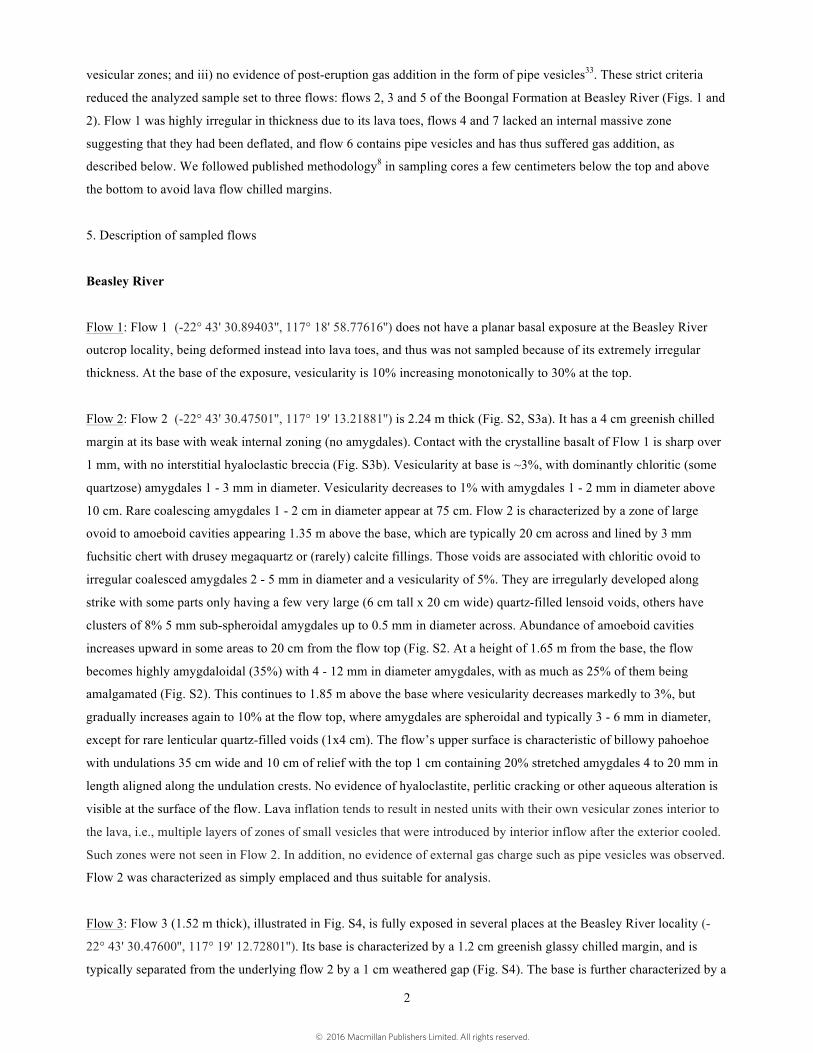
vesicular zones; and iii) no evidence of post-eruption gas addition in the form of pipe vesicles33. These strict criteria
reduced the analyzed sample set to three flows: flows 2, 3 and 5 of the Boongal Formation at Beasley River (Figs. 1 and
2). Flow 1 was highly irregular in thickness due to its lava toes, flows 4 and 7 lacked an internal massive zone
suggesting that they had been deflated, and flow 6 contains pipe vesicles and has thus suffered gas addition, as
described below. We followed published methodology8 in sampling cores a few centimeters below the top and above
the bottom to avoid lava flow chilled margins.
5. Description of sampled flows
Beasley River
Flow 1: Flow 1 (-22° 43' 30.89403'', 117° 18' 58.77616'') does not have a planar basal exposure at the Beasley River
outcrop locality, being deformed instead into lava toes, and thus was not sampled because of its extremely irregular
thickness. At the base of the exposure, vesicularity is 10% increasing monotonically to 30% at the top.
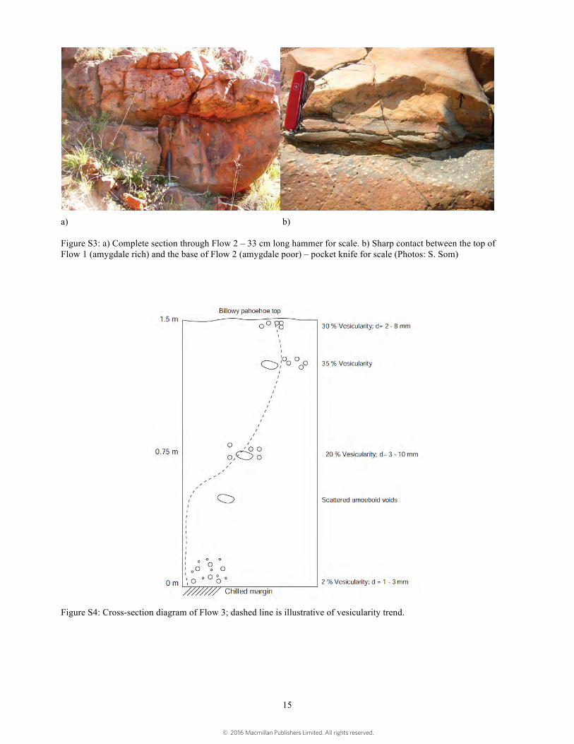
Flow 2: Flow 2 (-22° 43' 30.47501'', 117° 19' 13.21881'') is 2.24 m thick (Fig. S2, S3a). It has a 4 cm greenish chilled
margin at its base with weak internal zoning (no amygdales). Contact with the crystalline basalt of Flow 1 is sharp over
1 mm, with no interstitial hyaloclastic breccia (Fig. S3b). Vesicularity at base is ~3%, with dominantly chloritic (some
quartzose) amygdales 1 - 3 mm in diameter. Vesicularity decreases to 1% with amygdales 1 - 2 mm in diameter above
10 cm. Rare coalescing amygdales 1 - 2 cm in diameter appear at 75 cm. Flow 2 is characterized by a zone of large
ovoid to amoeboid cavities appearing 1.35 m above the base, which are typically 20 cm across and lined by 3 mm
fuchsitic chert with drusey megaquartz or (rarely) calcite fillings. Those voids are associated with chloritic ovoid to
irregular coalesced amygdales 2 - 5 mm in diameter and a vesicularity of 5%. They are irregularly developed along
strike with some parts only having a few very large (6 cm tall x 20 cm wide) quartz-filled lensoid voids, others have
clusters of 8% 5 mm sub-spheroidal amygdales up to 0.5 mm in diameter across. Abundance of amoeboid cavities
increases upward in some areas to 20 cm from the flow top (Fig. S2. At a height of 1.65 m from the base, the flow
becomes highly amygdaloidal (35%) with 4 - 12 mm in diameter amygdales, with as much as 25% of them being
amalgamated (Fig. S2). This continues to 1.85 m above the base where vesicularity decreases markedly to 3%, but
gradually increases again to 10% at the flow top, where amygdales are spheroidal and typically 3 - 6 mm in diameter,
except for rare lenticular quartz-filled voids (1x4 cm). The flow’s upper surface is characteristic of billowy pahoehoe
with undulations 35 cm wide and 10 cm of relief with the top 1 cm containing 20% stretched amygdales 4 to 20 mm in
length aligned along the undulation crests. No evidence of hyaloclastite, perlitic cracking or other aqueous alteration is
visible at the surface of the flow. Lava inflation tends to result in nested units with their own vesicular zones interior to
the lava, i.e., multiple layers of zones of small vesicles that were introduced by interior inflow after the exterior cooled.
Such zones were not seen in Flow 2. In addition, no evidence of external gas charge such as pipe vesicles was observed.
Flow 2 was characterized as simply emplaced and thus suitable for analysis.
Flow 3: Flow 3 (1.52 m thick), illustrated in Fig. S4, is fully exposed in several places at the Beasley River locality (-
22° 43' 30.47600'', 117° 19' 12.72801''). Its base is characterized by a 1.2 cm greenish glassy chilled margin, and is
typically separated from the underlying flow 2 by a 1 cm weathered gap (Fig. S4). The base is further characterized by a
© 2016 Macmillan Publishers Limited. All rights reserved.

3
low vesicularity of 2% with chloritic amygdales 1 - 3 mm in diameter. Scattered amoeboid quartz-filled voids (3 x 7
cm) appear 50 cm from the base. Vesicularity increases markedly at 75 cm to 20% with sub-spheroidal quartz-filled
amygdales 3-10 mm in diameter. This horizon is also characterized by amoeboid voids filled with quartz, fuchsitic
chert, chlorite, and calcite. Typical voids range from spheroidal 1 cm in diameter to amoeboid 3 x 10 cm. Vesicularity
increases to 35% within the top 30 cm. Amoeboid structures disappear in the top 10 cm of the flow, which has a
vesicularity of 30% with spheroidal quartz-filled amygdales 2 - 8 mm in diameter, located in a brown glassy margin.
The top of flow 3 is similar to flow 2, with billowy undulations 7 x 30 cm with 3 x 35 mm stretched amygdales in outer
centimeter that are aligned along crest axes. No evidence of multiple layers of zones of small vesicles characteristic of
lava inflation was found. Furthermore, the flow was devoid of pipe vesicles characteristic of external gas charge. As
such, Flow 3 was characterized as simply emplaced and suitable for analysis.
Flow 4: Flow 4 (1.78 m thick), illustrated in Fig. S5, is fully exposed in two places at the Beasley River locality
(-22° 43' 30.57293'', 117° 19' 13.04375''). Similar to Flow 3, it has a 1 cm erosional gap between its base and the top of
Flow 3. There is no evidence of a chilled margin, and the flow base is characterized by a vesicularity of 3%, with
spheroidal chloritic amygdales 1 - 3 mm in diameter. This distribution in size and vesicularity is found up to 80 cm
above the base, where large (5 x 12cm) lensoid to amoeboid voids filled with quartz-fuchsitic chert and calcite appear in
a 25 cm thick zone. These voids occupy 5% of this horizon, but are not interconnected. Vesicularity increases in this
same horizon to 5% with amygdales 3 - 5 mm in diameter. The large voids disappear in the top 50 cm but 1 - 2 cm in
diameter amoeboid amalgamated vesicles become common, forming 5% of the rock, while 20% is occupied by
spheroidal vesicles 3 - 6 mm in diameter. Vesicularity increases in the top 15 cm to 25%, where spheroidal quartzose
and chloritic amygdales 2 - 5 mm in diameter prevail in the absence of coalesced amygdales. The top surface of the
flow is somewhat foliated parallel to bedding, and no stretched amygdales are evident. The surface is very flat (relief
0.5 cm) compared with the underlying flows, and no hyaloclastite, cracking or perlitic fractures are observed. The fact
that this flow does not have a massive zone suggests that this flow was not simply emplaced, perhaps having suffered
deflation, and so it was deemed unsuitable for analysis.
Flow 5: Flow 5 (0.93 m thick), illustrated in Fig. S6, is fully exposed in one location (-22° 43' 30.44299'', 117° 19'
12.97333''). Its base has a 5 cm erosional gap with chalcedony veins (0.5 cm wide), but no evidence of a chilled margin.
The basal few centimeters of the flow is further characterized by 3% spheroidal chloritic amygdales1 - 3 mm in
diameter, passing upward into a sparsely amygdaloidal massive zone. At a height of 45 cm above the base, scattered
amoeboid to lenticular quartz-chlorite filled voids occupy 5% of rock, the largest void being 5 x 10 cm, but none are
interconnected. At that same level, sub-spheroidal amygdales 2 - 4 mm in diameter increase to 5% of the rock. At 65 cm
above the base, the large voids disappear and vesicularity increases to 10%, with sub-spheroidal quartzose and chloritic
amygdales 3 - 8 mm in diameter. This same horizon is also characterized by quartz-chlorite filled amoeboid (1 x 2 cm)
coalesced amygdales with a vesicularity of 2%. Vesicularity increases in the top 5 cm to 20% with spheroidal
amygdales 3 - 6 mm in diameter, and no amoeboid voids are present. Stretched amygdales are absent from the flow’s
top surface. It is nearly planar (3 cm relief), with no hyaloclastite or perlitic fracturing. Flow 5 is overlain by Flow 6,
which is at least 7.3 m thick, but disappears into a rubbly outcrop. Like Flows 2 and 3, Flow 5 lacked nested units
containing individual vesicular zones interior to the lava flow. In addition no sources of external gas charge like pipe
vesicles were observed. Flow 5 was thus characterized as simply emplaced and suitable for analysis.
© 2016 Macmillan Publishers Limited. All rights reserved.
4
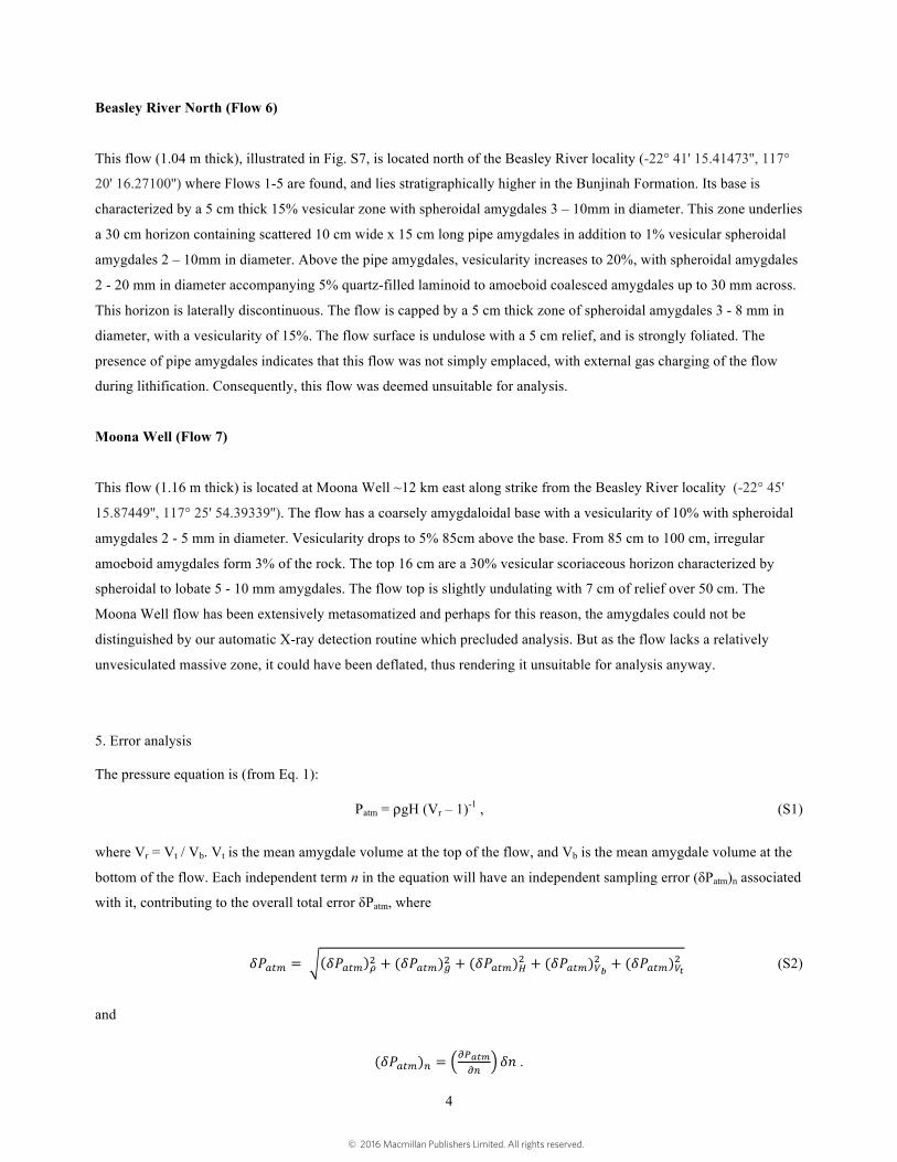
Beasley River North (Flow 6)
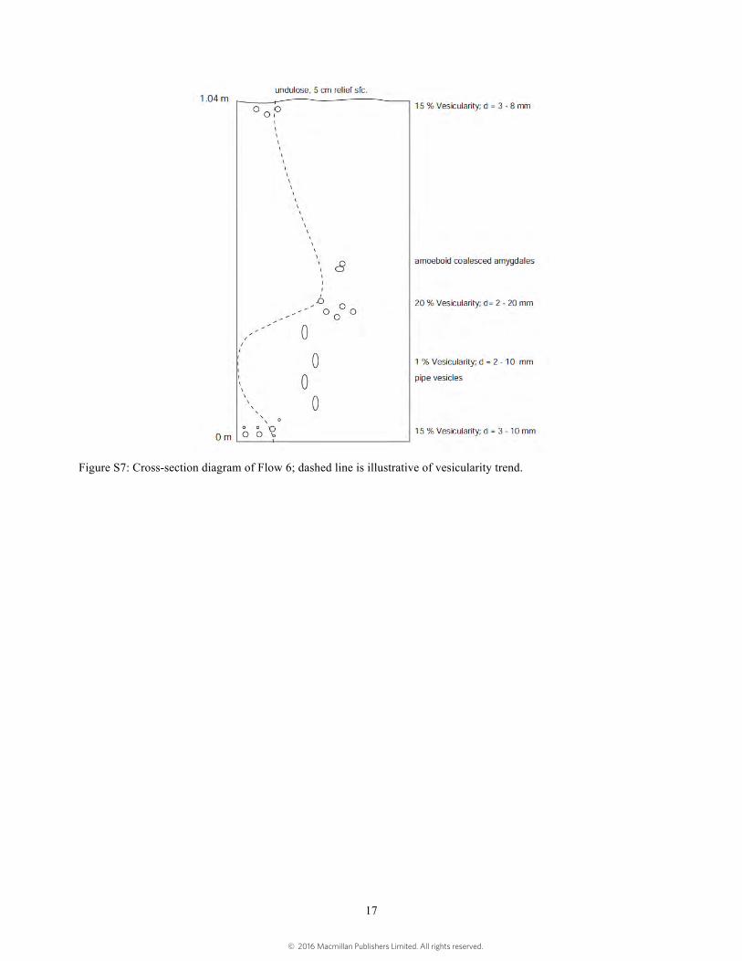
This flow (1.04 m thick), illustrated in Fig. S7, is located north of the Beasley River locality (-22° 41' 15.41473'', 117°
20' 16.27100'') where Flows 1-5 are found, and lies stratigraphically higher in the Bunjinah Formation. Its base is
characterized by a 5 cm thick 15% vesicular zone with spheroidal amygdales 3 – 10mm in diameter. This zone underlies
a 30 cm horizon containing scattered 10 cm wide x 15 cm long pipe amygdales in addition to 1% vesicular spheroidal
amygdales 2 – 10mm in diameter. Above the pipe amygdales, vesicularity increases to 20%, with spheroidal amygdales
2 - 20 mm in diameter accompanying 5% quartz-filled laminoid to amoeboid coalesced amygdales up to 30 mm across.
This horizon is laterally discontinuous. The flow is capped by a 5 cm thick zone of spheroidal amygdales 3 - 8 mm in
diameter, with a vesicularity of 15%. The flow surface is undulose with a 5 cm relief, and is strongly foliated. The
presence of pipe amygdales indicates that this flow was not simply emplaced, with external gas charging of the flow
during lithification. Consequently, this flow was deemed unsuitable for analysis.
Moona Well (Flow 7)
This flow (1.16 m thick) is located at Moona Well ~12 km east along strike from the Beasley River locality (-22° 45'
15.87449'', 117° 25' 54.39339''). The flow has a coarsely amygdaloidal base with a vesicularity of 10% with spheroidal
amygdales 2 - 5 mm in diameter. Vesicularity drops to 5% 85cm above the base. From 85 cm to 100 cm, irregular
amoeboid amygdales form 3% of the rock. The top 16 cm are a 30% vesicular scoriaceous horizon characterized by
spheroidal to lobate 5 - 10 mm amygdales. The flow top is slightly undulating with 7 cm of relief over 50 cm. The
Moona Well flow has been extensively metasomatized and perhaps for this reason, the amygdales could not be
distinguished by our automatic X-ray detection routine which precluded analysis. But as the flow lacks a relatively
unvesiculated massive zone, it could have been deflated, thus rendering it unsuitable for analysis anyway.
5. Error analysis The pressure equation is (from Eq. 1):
Patm = ρgH (Vr – 1)-1 , (S1)
where Vr = Vt / Vb. Vt is the mean amygdale volume at the top of the flow, and Vb is the mean amygdale volume at the
bottom of the flow. Each independent term n in the equation will have an independent sampling error (δPatm)n associated
with it, contributing to the overall total error δPatm, where
𝛿𝑃!"# = 𝛿𝑃!"# !! + (𝛿𝑃!"#)!! + (𝛿𝑃!"#)!! + (𝛿𝑃!"#)!!
! + (𝛿𝑃!"#)!!! (S2)
and
(𝛿𝑃!"#)! =!!!"#!"
𝛿𝑛 .
© 2016 Macmillan Publishers Limited. All rights reserved.

5
As such, each element in eq. S2 can be expressed as (S3a-e):
(𝛿𝑃!"#)! =𝜕𝑃!"#𝜕𝜌
𝛿𝜌 =𝑔𝐻𝑉!𝑉!− 1
𝛿𝜌
(𝛿𝑃!"#)! =𝜕𝑃!"#𝜕𝜌
𝛿𝑔 =𝜌𝐻𝑉!𝑉!− 1
𝛿𝑔
(𝛿𝑃!"#)! =𝜕𝑃!"#𝜕𝜌
𝛿𝐻 =𝜌𝑔
𝑉!𝑉!− 1
𝛿𝐻
(𝛿𝑃!"#)!! =𝜕𝑃!"#𝜕𝑉!
𝛿𝑉! = −𝜌𝑔𝐻
𝑉!𝑉!𝑉!− 1
! 𝛿𝑉!
(𝛿𝑃!"#)! =𝜕𝑃!"#𝜕𝑉!
𝛿𝑉! =𝑉!𝜌𝑔𝐻
𝑉!!𝑉!𝑉!− 1
! 𝛿𝑉!
where δρ, δg, δH, δVb and δVt are the measurement errors. The acceleration due to gravity g is obviously known to high
accuracy, so we assign δg = 0. We further set δρ = 100 kg m-3, and a conservative δH = 5% of lava flow thickness H to
account for the variability in thickness observed in the field.
Here we describe how to calculate δVb and δVt. The distribution of the volume of vesicles in basalts is generally found
to be close to log-normal34 and, as shown below, we find that our distributions also form an approximately log-normal
distribution. The physics of why the distribution of gas bubbles best fit the log-normal has been discussed to some
extent elsewhere (see references in Ref. 34). In essence, there is a fixed linear growth factor when vesicles form. So, the
bubbles that randomly grow larger than average will be a factor of ‘x’ larger (multiplicative), whereas the ones that
randomly grow smaller than average will be a factor of 'x’ smaller (divisional). This results in an approximately log-
normal distribution about the mean. In contrast, a linear normal distribution is where the random perturbations about a
mean are additive or subtractive (not multiplicative or divisional).
Standard statistical techniques require data that are normal (or Gaussian). Because the vesicle volume data tend to be
roughly log-normal, Proussevitch et al.34 recommend converting vesicular volumes to their logarithms, which converts
the roughly log-normal distributions to roughly normal distributions. Each distribution plotted in Figs S12 – S14 is
accompanied by a normal quantile plot that graphically represents how close the distribution is to normality, with a
correlation coefficient r = 0.9976 being the critical correlation coefficient (from NIST statistical tables) required to
accept the null hypothesis that the data came from a normal distribution. Those plots show that most outcrop
distributions cannot be statistically determined to come from a normal distribution, making the use of standard
statistical theory difficult. Consequently, we use bootstrap statistics to estimate the mean vesicle volume from the
roughly normal distribution30. Applying 2000 bootstrap resamples and plotting their means reveal, from the resulting
normal quantile plots (plotted in Figs S12 – S14), that the distribution of the mean of means is normal, (verifying the
© 2016 Macmillan Publishers Limited. All rights reserved.

6
Central Limit Theorem), and allowing the use of standard statistical theory such as the ~2σ spread for the 95%
confidence interval. The mean of this latter distribution is the best estimate for the mean of amygdale population, and
the standard deviation a measure of its error30. This error associated with the mean vesicle volume can then be used with
other sources of error in standard error propagation (which assumes normally-distributed errors) as discussed above.
Our MATLAB code for the bootstrapping is available in the online Supplementary Information. If large (or small)
vesicles skew the mean from the mode do exist in the original dataset, they will simply increase the standard deviation
of the Gaussian representing the mean of 2000 sample means. Outliers are thus taken into account in the statistics.
Converting these results back to linear space is the last step to obtain δVb and δVt. The calculation is as follows17:
Let µ equal the mean of the means of the bootstrapped distributions at either the flow top or bottom, and σµ the standard
deviation of that Gaussian. Let log(Vm) = µ, where Vm is the population mean in linear space, from which:
Vm = 10µ. (S4)
The error δVt,b in Vm due to the error σµ in µ is then expressed as:
δVt,b = { [ (∂Vm/∂µ)σµ ]2 }1/2 (S5)
The term (∂Vm/∂µ) can be written as 10µln(10) from the relationship:
∂ax/∂x = axln(a) (S6)
where a is a constant and x is a generic independente variable. Therefore, the volumetric error in the mean is expressed
as:
δVt,b = 10µln(10)σµ (S7)
Eqn. S7 corrects a typo in eqn. 10 of Ref. 17.
This method of error calculation is preferred because it produces a single standard deviation value when back-
transforming from logarithmic to linear, which can be inserted as δVb and δVt in eqn. S3d,e. Another method involves
back-transforming the error upper bound (mean + standard deviation) independently from the error lower bound (mean
– standard deviation), creating asymmetric error bars in the linear domain, making error propagation calculations
challenging. For the 95% confidence interval, we multiply the standard deviation by 1.96 (i.e., ≈2σ):
Vm_upper = (S8a)
Vm_lower = (S8b)
10 Vm+1.96σ µ( )
10 Vm−1.96σ µ( )
© 2016 Macmillan Publishers Limited. All rights reserved.
7
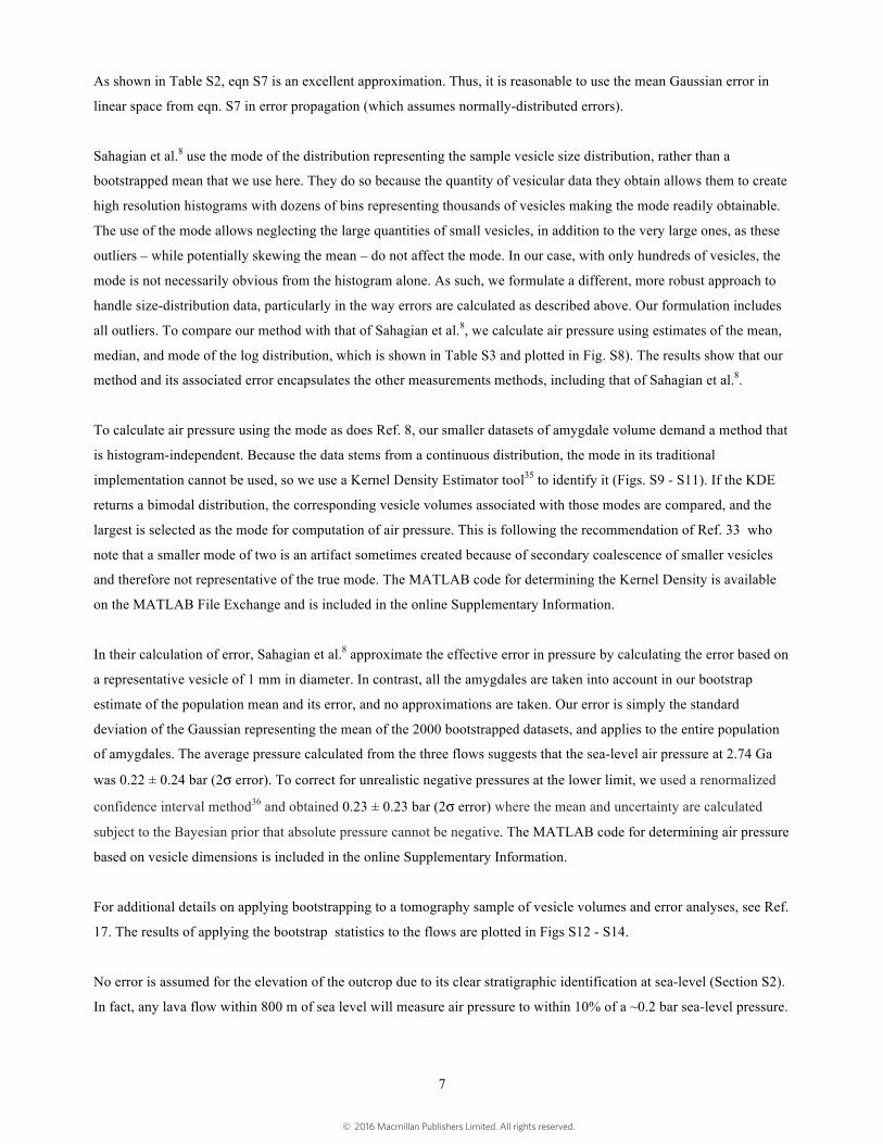
As shown in Table S2, eqn S7 is an excellent approximation. Thus, it is reasonable to use the mean Gaussian error in
linear space from eqn. S7 in error propagation (which assumes normally-distributed errors).
Sahagian et al.8 use the mode of the distribution representing the sample vesicle size distribution, rather than a
bootstrapped mean that we use here. They do so because the quantity of vesicular data they obtain allows them to create
high resolution histograms with dozens of bins representing thousands of vesicles making the mode readily obtainable.
The use of the mode allows neglecting the large quantities of small vesicles, in addition to the very large ones, as these
outliers – while potentially skewing the mean – do not affect the mode. In our case, with only hundreds of vesicles, the
mode is not necessarily obvious from the histogram alone. As such, we formulate a different, more robust approach to
handle size-distribution data, particularly in the way errors are calculated as described above. Our formulation includes
all outliers. To compare our method with that of Sahagian et al.8, we calculate air pressure using estimates of the mean,
median, and mode of the log distribution, which is shown in Table S3 and plotted in Fig. S8). The results show that our
method and its associated error encapsulates the other measurements methods, including that of Sahagian et al.8.
To calculate air pressure using the mode as does Ref. 8, our smaller datasets of amygdale volume demand a method that
is histogram-independent. Because the data stems from a continuous distribution, the mode in its traditional
implementation cannot be used, so we use a Kernel Density Estimator tool35 to identify it (Figs. S9 - S11). If the KDE
returns a bimodal distribution, the corresponding vesicle volumes associated with those modes are compared, and the
largest is selected as the mode for computation of air pressure. This is following the recommendation of Ref. 33 who
note that a smaller mode of two is an artifact sometimes created because of secondary coalescence of smaller vesicles
and therefore not representative of the true mode. The MATLAB code for determining the Kernel Density is available
on the MATLAB File Exchange and is included in the online Supplementary Information.
In their calculation of error, Sahagian et al.8 approximate the effective error in pressure by calculating the error based on
a representative vesicle of 1 mm in diameter. In contrast, all the amygdales are taken into account in our bootstrap
estimate of the population mean and its error, and no approximations are taken. Our error is simply the standard
deviation of the Gaussian representing the mean of the 2000 bootstrapped datasets, and applies to the entire population
of amygdales. The average pressure calculated from the three flows suggests that the sea-level air pressure at 2.74 Ga
was 0.22 ± 0.24 bar (2σ error). To correct for unrealistic negative pressures at the lower limit, we used a renormalized
confidence interval method36 and obtained 0.23 ± 0.23 bar (2σ error) where the mean and uncertainty are calculated
subject to the Bayesian prior that absolute pressure cannot be negative. The MATLAB code for determining air pressure
based on vesicle dimensions is included in the online Supplementary Information.
For additional details on applying bootstrapping to a tomography sample of vesicle volumes and error analyses, see Ref.
17. The results of applying the bootstrap statistics to the flows are plotted in Figs S12 - S14.
No error is assumed for the elevation of the outcrop due to its clear stratigraphic identification at sea-level (Section S2).
In fact, any lava flow within 800 m of sea level will measure air pressure to within 10% of a ~0.2 bar sea-level pressure.
© 2016 Macmillan Publishers Limited. All rights reserved.

8
6. Estimates of modern geological N fluxes
The Phanerozoic geological nitrogen fluxes in the main text were estimated using the N/C ratio of various carbon
reservoirs or outgassing fluxes and applying the N/C ratio as a scaling factor to well-known carbon fluxes19. Global
carbon fluxes are the most studied of any chemical element, so our approach gives N flux estimates with uncertainties.
However, the subduction flux of N and the mid-ocean ridge flux of N described in detail below were literature estimates
that used other techniques. In the Phanerozoic, the key geologic N source fluxes are outgassing (volcanic and
metamorphic) and oxidative weathering of continental organic matter, which releases nitrate that undergoes biological
denitrification essentially instantaneously on geologic timescales. The N sink flux is through the burial of organic
matter. A key conceptual point is that the only forms of N that can accumulate in the long term (over geologic
timescales) are N2 in the atmosphere or reduced N in rocks. The biosphere is a tiny, transient reservoir. It is for this
reason that we must consider oxidative weathering and rapid denitrification as an N source to the atmosphere on
geologic timescales.
We estimate the N outgassing flux as follows. A literature review37 indicates that the average CO2 outgassing from all
sources is 7 ± 3 Tmol C/yr (see in particular Table 4.1 in Ref. 37 ). Based on directly measured average N/C ratios in
subaerial volcanic and metamorphic gas emissions19, the N flux outgassing from arcs, hotspots, and metamorphism is
0.17 ± 0.07 Tmol N/yr, scaling from the C outgassing flux. Additionally, 0.008 ± 0.003 Tmol N/yr is outgassed from
mid-ocean ridges, according to helium-nitrogen systematics38. The total N outgassing flux from the sum of these
components is 0.18 ± 0.07 Tmol N/yr.
We estimate N burial and N weathering fluxes as follows. Analyses of sedimentary geochemical data reveal estimates
of the organic carbon oxidative weathering flux as 7.5 ± 1.7 Tmol/yr and organic carbon burial flux as 10 ± 1.7
Tmol/yr27. Based on N/C data for Phanerozoic shales and continental organics19, we estimate the weathering N flux as
0.15 ± 0.03 Tmol N/yr and the organic burial N flux as 0.4 ± 0.2 Tmol N/yr. The fraction of buried N that goes into
subduction zones is relatively small20, 0.094 ± 0.015 Tmol N/yr (compared to a value of 0.16 Tmol N/yr estimated in
Ref. 39) and within the noise of the uncertainty of the organic burial N sink. The net subduction flux is within error bar
of zero, if we take the value of Ref. 39 for the flux of N fed into subduction zones.
Overall, the total N source flux (0.33 ± 0.08 Tmol N/yr) and N sink flux (0.4 ± 0.2 Tmol N/yr) balance within the
uncertainty. In fact, modeling suggests that the Phanerozoic mass of N2 in the atmosphere probably varied < 1% 19.
The main text discusses the key differences in the anoxic Archaean. Firstly, there are convincing reasons why the N
source flux was smaller than today. The lack of an N oxidative weathering flux meant that the total N source flux would
have been halved based on the fluxes given above. Possibly (but very speculatively), the degassing of N was smaller too
if the source regions for gases from arc volcanism were at a lower redox state than today because this would stabilize
nitrogen in silicates against volatilization29. Secondly, in steady state balance, the global N sink flux must have been
smaller to balance a relatively diminished N source flux. Analysis of the carbon isotope record shows that organic
carbon burial is consistent with a smaller N sink in the Archaean as follows: in a generalized least squares analysis of C
© 2016 Macmillan Publishers Limited. All rights reserved.

9
isotopes, the fraction of carbon buried shows an increase of ~30% from the Archaean (0.15 ± 0.01 at 3.8-2.5 Gyr ) to the
Phanerozoic (0.22 ± 0.02 at 0.54-0 Gyr)40. Assuming the same N/C scaling, the Archaean N sink from organic burial
may have been similarly smaller by ~30% compared to the Phanerozoic. Clearly, this is smaller than the minimum
expected decrease of the N source flux (~50%). However, in the Archaean there would be a significant sink that is
absent in today’s oxygenated world. Ammonium, would be the dominant nitrogen species in the anoxic deep sea27.
Ammonium can readily substitute for potassium ions in clay minerals and provides a path for N to be transferred into
the solid Earth41. Biological anaerobic ammonium oxidation (“anammox”) is a pathway that in principle could oxidize
ammonium directly to nitrogen. However, this mechanism requires nitrite (NO2-), which would have been negligible in
the Archaean deep ocean (as it is in the modern Black Sea). Furthermore, ammonium-rich Archaean metasediments26,28
indicate that N2 released by anammox was negligible. Consequently, a considerable increase in the fraction of nitrogen
that entered crustal minerals and was subducted could make up the balance of the N sink flux. Nitrogen-enriched ~3.5
Gyr placer diamonds may record this period of high N subduction42. Importantly, because such a nitrogen sink should
depend on the concentration of N in the atmosphere-ocean system, the steady-state balance of N sources and sinks
would tend to favor lower pN2 in the atmosphere than today.
7. Nitrogen draw-down
We considered both abiotic and biological mechanisms that may have been responsible for sequestering nitrogen from
the early Earth’s atmosphere. Today it is estimated that there is ~2.1±1 bar of N2 in the mantle and crust4 with only 0.8
bar of N2 in the air. Most mantle nitrogen probably degassed during the first 200 Myr of Earth’s history from a magma
ocean21 because of its low solubility in silicate melts43. Some was evidently later removed from the air and returned to
the solid Earth.
Non-biological atmospheric nitrogen removal processes include fixation by lightning22, and HCN formation and
deposition23. In an anoxic atmosphere, N2 reacts with CO2 under the influence of lightning to form nitric oxide (NO)
and carbon monoxide (CO) (Ref. 22). Subsequently, NO further reacts to form a soluble nitrosyl hydride (HNO), which
can rain out of the atmosphere and disproportionate into forms of nitrogen that can be sequestered by burial44. However,
the flux of nitrogen fixed by lightning is very low, not more than 0.021 Tmol N/yr depending on the CO2 mixing ratio22.
If this abiotic nitrogen fixation flux was uniform for the 1.8 Gyr from Earth’s origin to Boongal deposition with none
returning to the atmosphere, this mechanism could only sequester ~0.1 bar of N2. The other abiotic draw-down
mechanism via HCN arises from N atoms that react with methylene (CH2) and methyl (CH3) radicals derived from the
photolysis of methane23. Although the reaction-rate constants are uncertain, the nitrogen removal rate is estimated to be
small, similar to that by lightning24. Thus, the fluxes of purely abiotic fixed nitrogen are evidently insufficient to explain
low atmospheric pN2 during the late Archaean.
A hypothesis for why the early atmosphere (before 2.7 Gyr ago) may have lost N2 relative to today is as follows. In the
Archaean ocean, the dominant form of N in seawater was ammonium, given anoxic geochemical speciation1,27 and
enhanced levels of ammonium in marine sediments that are inferred to have been derived from clay minerals26,28.
Biological nitrogen fixation has been proposed to date back even to the last common ancestor of extant life based on
phylogenetics45, although that idea is controversial and disputed. Nonetheless, given the antiquity of biological nitrogen
© 2016 Macmillan Publishers Limited. All rights reserved.

10
fixation going back to 3.2 Gyr25 or even 3.8 Gyr26 from geochemical evidence, atmospheric nitrogen gas would be
efficiently transformed to dissolved ammonium by microbial ammonification after biological fixation. The estimated
modern N fixation flux is > 1.43 Tmol N/yr, for example24. Seawater ammonium can be incorporated into phyllosilcate
minerals because it substitutes for K+, which ultimately transfers to other silicates46,47. Ammonium in silicates is
refractory during high temperature processes unlike carbon46, which returns to the atmosphere as CO2 or CH4 in a faster
geologic cycle than nitrogen. Thus, nitrogen could plausibly have been sequestered into crustal and mantle minerals on
the early Earth, leaving a thinner atmosphere than today.
We can gain additional insight from estimates of fluxes. Today, the input of N into subduction zones is estimated as
~0.094 Tmol N/yr20. If this flux were an order of magnitude greater in the Archaean due to efficient ammonium sinks
into phyllosilicates, and all the ammonium entered the mantle, then the residence time of the equivalent present
atmospheric level of nitrogen (2.8 × 10⁸ Tmol N) against subduction would be 0.3 Gyr. It is reasonable to assume that in
the absence of atmospheric oxygen the source of nitrogen released from oxidative weathering of organic matter would
be greatly diminished compared to today’s flux of ~0.15 Tmol N/yr19. However, outgassing (currently ~0.33 Tmol N/yr)
would have maintained pN2 at some lower level than today in dynamic balance.
The oxygenation of the atmosphere at ~2.4 Gyr likely caused a return of nitrogen to the atmosphere and, because the
dominant form of N in the ocean changed to nitrate, the pathway to lose N to ammonium silicates was also diminished.
The most obvious new source of N was oxidative weathering of organic material on the continents, releasing nitrate to
rivers and the ocean where biological denitrification would return N2 to the atmosphere. As mentioned above, oxidative
weathering releases N from organic carbon19 with a flux that we estimate as ~0.15 Tmol N/year. A more speculative
possibility is that following the Great Oxidation Event (GOE), newly available oxidized species like Fe3+ and sulfates
made their way to the mantle wedge by subduction48, which may have shifted the redox balance allowing nitrogen to
speciate from NH4+, which tends to stay in the solid phase, to N2, which tends to be released to the atmosphere29. Thus,
the flux of N2 from arc volcanism may have increased as a feedback effect of the GOE if the source region’s redox state
changed. One can estimate, based on modern fluxes, how long a return to a 0.8 bar pN2 would take from a N2 dominant
0.5 bar atmosphere. Modern outgassing of nitrogen is ~0.18 Tmol N/year, which when summed with the flux from
oxidative weathering, gives a release of ~0.33 Tmol N/year (following Ref. 19). Thus, ~0.3 bar N2 (~1.08×10⁸ Tmol N
following Ref. 49) would be replenished in ~330 million years. This value is conservative because outgassing rates were
likely greater in the Archaean owing to a hotter lithosphere and mantle. It is interesting that this duration would coincide
with the time of 2.4-2.0 Gyr ago when there were major fluctuations in climate and the global carbon cycle, before the
Earth system settled into the Proterozoic eon.
Overall, early Archaean (or even Hadean) burial of substantial quantities of biologically fixed nitrogen would support
the hypothesis of Goldblatt et al.4 that the nitrogen present in the mantle today was in the atmosphere at some point very
early in Earth’s history, but not as late as 2.7 Gyr.
© 2016 Macmillan Publishers Limited. All rights reserved.

11
References for Supplementary Materials
31. Cas, R. & Wright, J. V. Volcanic Successions, modern and ancient: a geological approach to processes, products, and successions. (Allen & Unwin, 1987).
32. Blake, T. S., Buick, R., Brown, S. J. a. & Barley, M. E. Geochronology of a Late Archaean flood basalt province in the Pilbara Craton, Australia: constraints on basin evolution, volcanic and sedimentary accumulation, and continental drift rates. Precambrian Res. 133, 143–173 (2004).
33. Sahagian, D. & Proussevitch, A. Paleoelevation Measurement on the Basis of Vesicular Basalts. Reviews in Mineralogy and Geochemistry 66, 195–213 (2007).
34. Proussevitch, A. Statistical analysis of bubble and crystal size distributions: Formulations and procedures. J. Volcanol. Geotherm. Res. 164, 95–111 (2007).
35. Botev, Z., Grotowski, J. & Kroese, D. Kernel density estimation via diffusion. Ann. Stat. 38, 2916–2957 (2010).
36. Cowen, S. & Ellison, S. L. R. Measurement uncertainty and confidence intervals near natural limits. Analyst 131, 710–717 (2006).
37. Berner, R. a. The Phanerozoic carbon cycle: CO2 and O2. (Oxford University Press, 2004).
38. Marty, B. & Zimmermann, L. Volatiles (He, C, N, Ar) in mid-ocean ridge basalts: Assesment of shallow-level fractionation and characterization of source composition. Geochim. Cosmochim. Acta 63, 3619–3633 (1999).
39. Johnson, B. & Goldblatt, C. The Nitrogen Budget of Earth. Earth-Science Rev. 148, 150–173 (2015).
40. Krissansen-Totton, J. A statistical analysis of the carbon isotope record from the Archean to Phanerozoic and implications for the rise of oxygen. Am. J. Sci. 315, 275–316 (2015).
41. Watenphul, A., Wunder, B. & Heinrich, W. High-pressure ammonium-bearing silicates: Implications for nitrogen and hydrogen storage in the Earth’s mantle. Am. Mineral. 94, 283–292 (2009).
42. Smart, K. A., Tappe, S., Stern, R. A., Webb, S. J. & Ashwal, L. D. Early Archaean tectonics and mantle redox recorded in Witwatersrand diamonds. Nat. Geosci. 1–6 (2016). doi:10.1038/NGEO2628
43. Wen, J. S., Pinto, J. P. & Yung, Y. L. Photochemistry of CO and H2O: analysis of laboratory experiments and applications to the prebiotic Earth’s atmosphere. J. Geophys. Res. 94, 14957–70 (1989).
44. Catling, D. & Kasting, J. in Planets and Life: The Emerging Science of Astrobiology (eds. Sullivan, W. T. & Baross, J. A.) 91–116 (Cambridge University Press, 2007).
45. Fani, R., Gallo, R. & Liò, P. Molecular evolution of nitrogen fixation: the evolutionary history of the nifD, nifK, nifE, and nifN genes. J. Mol. Evol. 51, 1–11 (2000).
46. Boyd, S. Ammonium as a biomarker in Precambrian metasediments. Precambrian Res. 108, 159–173 (2001).
47. Morse, J. & Morin, J. Ammonium interaction with coastal marine sediments: influence of redox conditions on K*. Mar. Chem. 95, 107–112 (2005).
48. Evans, K. The redox budget of subduction zones. Earth-Science Rev. 113, 11–32 (2012).
49. Trenberth, K. Global atmospheric mass, surface pressure, and water vapor variations. J. Geophys. Res. Atmos. 92, 14815–14826 (1987).
© 2016 Macmillan Publishers Limited. All rights reserved.
12
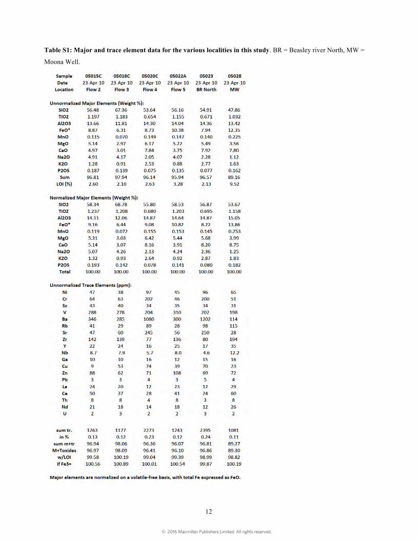
Table S1: Major and trace element data for the various localities in this study. BR = Beasley river North, MW =
Moona Well.
© 2016 Macmillan Publishers Limited. All rights reserved.

13
Table S2: Two methods of calculating errors. All values in mm3
. Only values for Upper Vesicular Zone shown. This table shows that transformation of the standard deviation from logarithmic to linear using Eq. 7 is a good approximation to the asymmetrical result (Eq. S8). The “single-value” is preferred as it allows effective error propagation in the calculation of air pressure error (Eq. S2, S3d,e)
Table S3: Atmospheric pressure of each flow using different parameters. Air pressure is calculated given the mean, median and mode of the logarithmic distribution of amygdale sizes.
Flow # Patm [bar] (log data) Patm (bootstrap method)
Mean Median Mode
2 0.14 0.12 0.06 0.14 3 0.11 0.12 0.08 0.11 5 0.40 0.38 0.05 0.39
Flow #F Flow # Vm (Eq. S4)
Combined error 2σ
(2 x Eq. S7)
Upper-bound error
(Eq. S8a)
Lower-bound error
(Eq. S8b) 2 2.24 0.28 0.29 0.25 3 2.85 0.57 0.62 0.51 5 0.98 0.17 0.18 0.15
© 2016 Macmillan Publishers Limited. All rights reserved.

14
Figure S1: Geochemical results from the Beasley River samples overprinted on northern Pilbara results32.
Figure S2: Cross-section diagram of Flow 2; dashed lines are illustrative of vesicularity trends.
© 2016 Macmillan Publishers Limited. All rights reserved.
15
a) b) Figure S3: a) Complete section through Flow 2 – 33 cm long hammer for scale. b) Sharp contact between the top of Flow 1 (amygdale rich) and the base of Flow 2 (amygdale poor) – pocket knife for scale (Photos: S. Som)
Figure S4: Cross-section diagram of Flow 3; dashed line is illustrative of vesicularity trend.
© 2016 Macmillan Publishers Limited. All rights reserved.

16
Figure S5: Cross-section diagram of Flow 4; dashed line is illustrative of vesicularity trend.
Figure S6: Cross-section diagram of Flow 5; dashed line is illustrative of vesicularity trend.
© 2016 Macmillan Publishers Limited. All rights reserved.
17
Figure S7: Cross-section diagram of Flow 6; dashed line is illustrative of vesicularity trend.
© 2016 Macmillan Publishers Limited. All rights reserved.

18
Fig. S8: Illustration of Table S1 showing atmospheric pressure (Patm) results for each flow using different statistical
measures of the central tendency of the log-normal vesicle distributions from lava flows 2, 3 and 5. The different
statistical measures (see text) are labelled ‘log mean’, ‘log median’ and ‘log mode’, respectively. Using the method of a
bootstrap sampling distribution of the mean, the result from the three flows combined is a mean atmospheric pressure of
Patm = 0.23 bar with a 2σ uncertainty of 0.23 bar. This bootstrap estimate encompasses all the other estimates within its
2σ uncertainty (or 95% confidence interval)..
© 2016 Macmillan Publishers Limited. All rights reserved.

19
Figure S9. Flow 2: Histogram and Kernel Density Estimator of amygdale volumes from both the flow top (upper
panel), and flow bottom (lower panel). Density describes the likelihood for a random variable to take a given value. The
KDE is used to compute a mode for the distribution, and is determined without knowing a priori the parametric model
of the distribution. In the top panel, the rightmost mode is used because the leftmost one yields unphysical negative
pressures. Air pressure calculated using distribution modes is not the primary method used in this study – see text for
details.
© 2016 Macmillan Publishers Limited. All rights reserved.

20
Figure S10. Flow 3: Histogram and Kernel Density Estimator (KDE) of amygdale volumes from both the flow top
(upper panel), and flow bottom (lower panel). Density describes the likelihood for a random variable to take a given
value. The KDE is used to compute a mode for the distribution, and is determined without knowing a priori the
parametric model of the distribution. Air pressure calculated using distribution modes is not the primary method used in
this study – see text for details.
© 2016 Macmillan Publishers Limited. All rights reserved.

21
Figure S11. Flow 5: Histogram and Kernel Density Estimator of amygdale volumes from both the flow top (upper
panel), and flow bottom (lower panel). Density describes the likelihood for a random variable to take a given value. The
KDE is used to compute a mode for the distribution, and is determined without knowing a priori the parametric model
of the distribution. In the top panel, the rightmost mode is used because the leftmost one yields unphysical negative
pressures. Air pressure calculated using distribution modes is not the primary method used in this study – see text for
details.
© 2016 Macmillan Publishers Limited. All rights reserved.
22
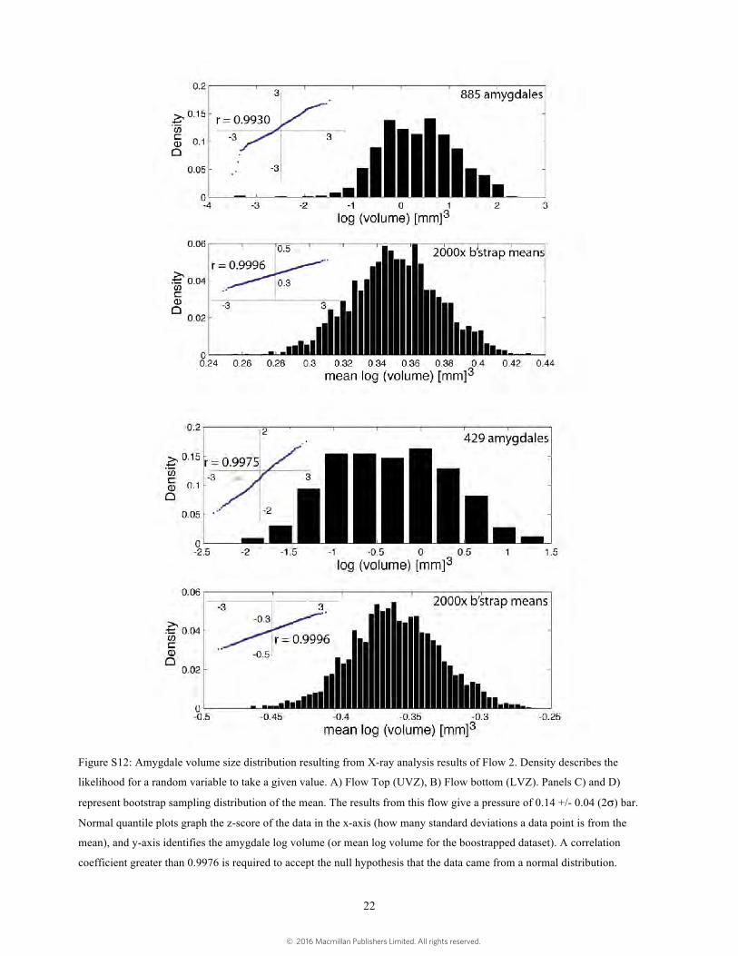
Figure S12: Amygdale volume size distribution resulting from X-ray analysis results of Flow 2. Density describes the
likelihood for a random variable to take a given value. A) Flow Top (UVZ), B) Flow bottom (LVZ). Panels C) and D)
represent bootstrap sampling distribution of the mean. The results from this flow give a pressure of 0.14 +/- 0.04 (2σ) bar.
Normal quantile plots graph the z-score of the data in the x-axis (how many standard deviations a data point is from the
mean), and y-axis identifies the amygdale log volume (or mean log volume for the boostrapped dataset). A correlation
coefficient greater than 0.9976 is required to accept the null hypothesis that the data came from a normal distribution.
© 2016 Macmillan Publishers Limited. All rights reserved.
23
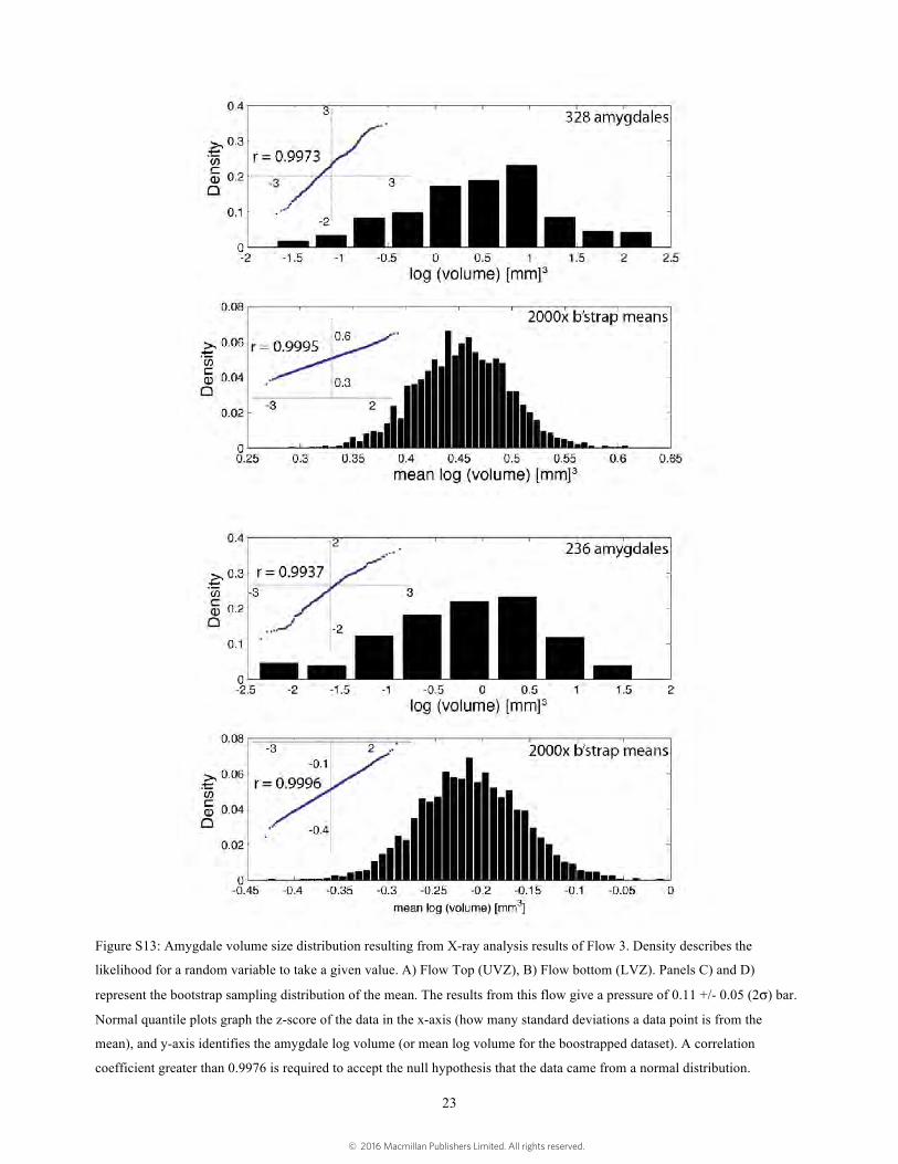
Figure S13: Amygdale volume size distribution resulting from X-ray analysis results of Flow 3. Density describes the
likelihood for a random variable to take a given value. A) Flow Top (UVZ), B) Flow bottom (LVZ). Panels C) and D)
represent the bootstrap sampling distribution of the mean. The results from this flow give a pressure of 0.11 +/- 0.05 (2σ) bar.
Normal quantile plots graph the z-score of the data in the x-axis (how many standard deviations a data point is from the
mean), and y-axis identifies the amygdale log volume (or mean log volume for the boostrapped dataset). A correlation
coefficient greater than 0.9976 is required to accept the null hypothesis that the data came from a normal distribution.
© 2016 Macmillan Publishers Limited. All rights reserved.

24
Figure S14: Amygdale volume size distribution resulting from X-ray analysis results of Flow 5. Density describes the
likelihood for a random variable to take a given value. A) Flow Top (UVZ), B) Flow bottom (LVZ). Panels C) and D)
represent the bootstrap sampling distribution of the mean. The results from this flow give a pressure of 0.40 +/- 0.23
(2σ) bar. Normal quantile plots graph the z-score of the data in the x-axis (how many standard deviations a data point is
from the mean), and y-axis identifies the amygdale log volume (or mean log volume for the boostrapped dataset). A
© 2016 Macmillan Publishers Limited. All rights reserved.

25
correlation coefficient greater than 0.9976 is required to accept the null hypothesis that the data came from a normal
distribution.
© 2016 Macmillan Publishers Limited. All rights reserved.