Embed Size (px)
Citation preview

www.pdfbo
oksfr
ee.pk
Presented by www.pdfbooksfree.pk

Earthquake Resistant Buildings
VISIT FOR MORE USEFUL BOOKSwww.pdfbooksfree.pkwww.pdfbooksfree.org
www.pdfbo
oksfr
ee.pk
Presented by www.pdfbooksfree.pk

www.pdfbo
oksfr
ee.pk
Presented by www.pdfbooksfree.pk

M.Y.H. Bangash
Earthquake ResistantBuildings
Dynamic Analyses, NumericalComputations, Codified Methods, CaseStudies and Examples
1 3
www.pdfbo
oksfr
ee.pk
Presented by www.pdfbooksfree.pk

M.Y.H. BangashConsulting Engineer in AdvancedStructural Analysis
London, UK
ISBN 978-3-540-93817-0 e-ISBN 978-3-540-93818-7DOI 10.1007/978-3-540-93818-7Springer Heidelberg Dordrecht London New York
Library of Congress Control Number: 2010920825
This work is subject to copyright. All rights are reserved, whether the whole or part of the material isconcerned, specifically the rights of translation, reprinting, reuse of illustrations, recitation,broadcasting, reproduction on microfilm or in any other way, and storage in data banks. Duplicationof this publication or parts thereof is permitted only under the provisions of theGermanCopyright Lawof September 9, 1965, in its current version, and permission for use must always be obtained fromSpringer. Violations are liable to prosecution under the German Copyright Law.The use of general descriptive names, registered names, trademarks, etc. in this publication does notimply, even in the absence of a specific statement, that such names are exempt from the relevantprotective laws and regulations and therefore free for general use.
Cover design: deblik, Berlin
Printed on acid-free paper
Springer is part of Springer Science+Business Media (www.springer.com)
# 2011 M.Y.H. Bangash; London, UKPublished by: Springer-Verlag Berlin Heidelberg 2011
www.pdfbo
oksfr
ee.pk
Presented by www.pdfbooksfree.pk
Preface
This book provides a general introduction to the topic of three-dimensional
analysis and design of buildings for resistance to the effects of earthquakes. It is
intended for a general readership, especially persons with an interest in the
design and construction of buildings under servere loadings.A major part of design for earthquake resistance involves the building
structure, which has a primary role in preventing serious damage or structural
collapse. Much of the material in this book examines building structures and,
specifically, their resistance to vertical and lateral forces or in combinations.
However, due to recent discovery of the vertical component of acceleration of
greater magnitude in the kobes’ earthquake the original concept of ‘‘lateral
force only’’ has changed. This book does advocate the contribution of this
disastrous component in the global analytical investigation.When the earthquake strikes, it shakes the whole building and its contents.
Full analysis for design layout and type of earthquakes, therefore, must include
considerations for the complete building construction, the building contents
and the building occupants.The work of designing for earthquake effects is formed by a steady stream of
studies, research, new technologies and the cumulative knowledge gained from
forensic studies of earthquake-damaged buildings. Design and construction
practices, regulating codes and professional standards continuously upgraded
due to the flow of this cumulative knowledge. Hence, any book on this subject
must regularly be updated. Since the effects are not the same, the earthquake
forces are always problematic.Over the years, earthquake has been the cause of great disasters in the form
of destruction of property and injury and loss of life to the population. The
unpredictability and sudden occurrence of earthquakes make them somewhat
mysterious, both to the general public and to professional building designers.
Until quite recently, design for earthquakes – if consciously considered at all –
was done with simplistic methods and a small database. Extensive study and
research and a great international effort and cooperation have vastly improved
design theories and procedures. Accordingly, most buildings in earthquake-
prone areas today are designed in considerable detail for seismic resistance.
v
www.pdfbo
oksfr
ee.pk
Presented by www.pdfbooksfree.pk
Despite the best efforts of scientists and designers, most truly effective designmethods are those reinforced by experience. This experience, unfortunately,grown by leaps when a major earthquake occurs and strongly affects regions ofconsiderable development – notably urban areas. Observation of damagedbuildings by experts in forensic engineering adds immeasurably to our knowl-edge base. While extensive research studies are ongoing in many testing labora-tories, the biggest laboratory remains the real world and real earthquakes.
Design decisions that affect the seismic response of buildings range frombroad to highly specific ones.While much of this design workmay be performedby structural engineers, many decisions aremade by, or are strongly affected by,others. Building codes and industry standards establish restrictions on the useof procedures for analysis of structural behaviour and for the selection ofmaterials and basic systems for construction. Decisions about site development,building placement on sites, building forms and dimensions and the selection ofmaterials and details for construction are often made by so many others too.
On this respect it was necessary that the reader should look into codes ofpractice in certain countries prone to major earthquakes. Some codes includingthe Eurocode-8 are given together with numerical and analytical methods forcomparative studies. This approach enhances the design quality and createsconfidence in the designer on his/her work.
While ultimate collapse of the Building structure is a principal concern, thebuilding’s performance during an earthquake must be considered in many otherways as well. If the structure remains intact, but structural part of the buildingsustains critical damage, occupants are traumatized or injured, and it is infeasibleto restore the building for continued use; the design work may not be viewed assuccess.However, the necessity sometimes governs. Some countriesmay not havesophisticated tools and resources. Others must assist to provide them.
The work in this book is mostly analytical and hence should be accessible tothe broad range of people in the building design and construction fields. Thiscalls for some compromise since all are trained highly in some areas and less – ornot at all – in others. The readers should have general knowledge of buildingcodes, current construction technology, principal problems of planning build-ings and at least an introduction to design of simple structures for earthquake-prone buildings. Most of all, readers need some real motivation for learningabout making buildings safer during earthquakes. Many design examples andcase studies are included to make the book fully attractive to all and sundry.
Readers less prepared may wish to strengthen their backgrounds in order toget the most from the work in this book. The author gives a vast bibliography atthe end of this book and a list of references after each chapter so that the readercan carryout an in-depth study on a specific area missed out in detail. Thereader hopefully will understand the need for grappling with this complexsubject.
This book addresses the perplexing problem of how to maintain operabilityof equipment after a major earthquake. The programme is often more compli-cated than simple anchorage. Some critical types of equipment, for example,
vi Preface
www.pdfbo
oksfr
ee.pk
Presented by www.pdfbooksfree.pk
are likely to fail operationally (false signalling of switches, etc.) even if adequatebase anchorage has been provided. It is the goal of this book to point out to thereader with a plan whereby equipment must be classified and subsequentlyqualified for the postulated seismic environment in a manner that best suitsthe individual piece of equipment. In some cases this qualification and analysiscan be accomplished only by sophisticated seismic testing programme, while atthe other end of the spectrum, equipment sometimes may be qualified simply byadequate architectural detailing. All too often, professional design teams andowners rely on an electric plug and gravity to keep a critical piece of equipmentin place during an earthquake and functional afterwards. Obviously, this is lessthan desirable situation. One part of the suggestion is devoted to the qualifica-tion procedures which include
� Testing� Analyses� Designer’s judgement� Prior experience� Design earthquakes� Seismic categories for equipment� Design specification procedures
The reader can easily be advised to refer to relevant codes such as Eurocode 8and its supplements and parts. This book does not go into details regarding theabove procedures but only concentrates on the analytical/design methodology.
The discussion of these topics leaves the designer with a complete course ofaction for qualifying all types of equipments, such as seismic devices to controlthe building structures during earthquakes. The author for this reason gives acomprehensive chapter on the subject.
One major measure to mitigate the earthquake hazards is to design and buildstructures through better engineering practices, so that these structures possessadequate earthquake-resistant capacity. Considerable research efforts havebeen carried out in the USA, Japan, China and other countries in the last fewdecades to advance earthquake engineering knowledge and design methods.This book summarizes the state-of-the-art knowledge and worldwide experi-ences, particularly those from China and the USA, and presents them system-atically in one volume for possible use by engineers, researchers, students, andother professionals in the field of earthquake engineering. Considering theactive research and rapid technological advances which have taken place inthis field, there has been a surprising shortage of suitable textbooks for seniorlevel or graduate level students. This book also attempts to help fill such a gap.
The book consists of 10 major parts: engineering seismology and earth-quake-resistant analyses and design. Special attention is placed on bridgingthe gap between these disciplines. For the convenience of the reader, funda-mentals of seismology, earthquake engineering and random processes, which,can be useful tools to describe the three-dimensional ground motions are givento assess the structural or soil response to them. Vast chapters are included.
Preface vii
www.pdfbo
oksfr
ee.pk
Presented by www.pdfbooksfree.pk

This is followed by describing earthquake intensity, ground motions and itsdamaging effects. In the ensuing chapters concerning the earthquake-resistantdesign, both fundamental theories and new research problems and designstandards are introduced. In this book stochastic methods are introducedbecause of their potential to offer a new dimension in earthquake engineeringapplications. These two areas have been subjected to intensive research in recentyears and there is a potential in them to provide solutions to some specialproblems which might not be amenable to conventional approaches. Appen-dices are given for supporting analyses. Computer subroutines, which can beused with any known packages to suit the reader.
Although this book may appear to present a daunting amount of material, itis, nevertheless, just a toe in the door of the vast library of knowledge that exists.Readers may use this book to gain general awareness of the field or to launch amuch more exhaustive programme of study.
On design sides, many codified methods have been briefly mentioned. TheEurocode EC-8 and the American codes with examples have been highlighted.
The book will serve as a useful text for teachers preparing design syllabi forundergraduate and postgraduate courses. Each major section contains a fullexplanation which allows the book to be used by students and practicingengineers, particularly those facing formidable task of having to design/detailcomplicated building structures with unusual boundary conditions. Contrac-tors will also find this book useful in the preparation of construction drawings,and manufacturers will be interested in the guidance even in the text recordingcodified and newly developed methods and the manufacture of earthquakeresistant devices.
London, UK M.Y.H. Bangash
viii Preface
www.pdfbo
oksfr
ee.pk
Presented by www.pdfbooksfree.pk

Acknowledgments
The author is indebted to many individuals, institutions, organizations and
research establishments mentioned in the text for helpful discussions and for
providing useful practical data and research materials.The author owes a special debt of gratitude to his family who, for the third
time, provided unwavering support.The author also acknowledges the following private communications:
Aerospace Daily (Aviation and Aerospace Research), 1156 15th Street NW,Washington, 20005, USA.
Azad Kashmir, Disaster Management Centre. Reports Jan. 2008–2009.Afghan Agency Press, 33 Oxford Street, London, UK.Agusta SpA, 21017 Cascina Costa di Samarate (VA), Italy.Ailsa Perth Shipbuilders Limited, Harbour Road, Troon, Ayrshire KA10
6DN, Scotland.Airbus Industrie, 1 Rond Point Maurice Bellonte, 31707 Blagnac Cedex,
France.Allison Gas Turbine, General Motors Corporation, Indianapolis, Indiana
46 206–0420, USA.AMX International, Aldwych House, Aldwych, London, WC2B 4JP, UK.Arizona State University, Tempe AZ, USA.AzadKashmir office for EarthquakeManagement Pakistan, 2009. Pakistan,
(Pukhtoon Khawa) N.W.F.P. Pakistan, Peshawar, Earthquake Division,2009, Pakistan
Bogazici, University, Turkey.Bremer Vulkan AG, Lindenstrasse 110, PO Box 750261, D-2820 Bremen 70,
Germany.British Library, Kingcross, London, UK.Catic, 5 Liang Guo Chang Road, East City District (PO Box 1671), Beijing,
China.Chantiers de l’Atlantique, Alsthom-30, Avenue Kleber, 75116 Paris, France.Chemical and Engineering News, 1155 16th Street NW, Washington DC
20036, USA.Chinese State Arsenals, 7A Yeutan Nanjie, Beijing, China.
ix
www.pdfbo
oksfr
ee.pk
Presented by www.pdfbooksfree.pk

Conorzio Smin, 52, Villa Panama 00198, Rome, Italy.CITEFA, Zufratequ y Varela, 1603 Villa Martelli, Provincia de Buenos
Aires, Argentina.Daily Muslim, Abpara, Islamabad, Pakistan.Daily Telegraph, Peterborough Court, South Quay Plaza, Marshwall,
London E14, UK.Dassault-Breguet, 33 Rue de Professeur Victor Pauchet, 92420, Vaucresson,
France.Defense Nationale, 1 Place Joffre, 75700, Paris, France.Der Spiegel, 2000 Hamburg 11, Germany.Department of Engineering Sciences, University of California, San Diego,
CA, USA.Earthquake Hazard Prevention Institute, Wasada University, Shinju Ko-Ku,
Tokyo, JapanEarthquake Research Institute, University of Tokyo, JapanEvening Standard, Evening Standard Limited, 118 Fleet Street, London
EC4P 4DD, UK.Financial Times, Bracken House, 10 Cannon Street, London EC4P 4BY.Fokker, Corporate Centre, PO Box 12222, 1100 AE Amsterdam Zuidoost,
The Netherlands.Fukuyama University, Gakuen-Cho, Fukuyama, Hiroshima, JapanGeneral Dynamic Corporation, Pierre Laclede Centre, St Louis, Missouri
63105, USA (2003–2009).General Electric, Neumann Way, Evendale, Ohio 45215, USA.Graduate School of Engineering, Kyoto University, Kyoto, JapanGuardian, Guardian Newspapers Limited, 119 Farringdon Road, Londo
EC1R 3ER, UK.Hawker Siddeley Canada Limited, PO Box 6001, Toronto AMF, Ontario
L5P 1B3, Canada.Hindustan Aeronautics Limited, Indian Express Building, PO Box 5150,
Bangalore 560 017, India (Dr Ambedkar Veedhil).Howaldtswerke DeutscheWerft, PO Box 146309, D-2300Kiel 14, Germany.Imperial College Earthquake Engineering Centre, London, U.K. The Indian
institute of Technology, Bombay, India (2009).Independent, 40 City Road, London EC1Y 2DB, UK. (2007–2009)Information Aeronautiques et Spatiales, 6 Rue Galilee, 75116, Paris, France.Information Resources Annual, 4 Boulevard de 1’Empereur, B-1000, Brus-
sels, Belgium.Institute Fur Ange Nandte Mechanik, Techniche Universitat Braunschweig.
D-38106, Braunschweig, Germany (2009).Institutodi Energetica, Universita degdi studi Reggio Calibria, Reggio,
Calibria, ItalyInternational Aero-engines AG, 287Main Street, East Hartford, Connecticut
06108, USA.
x Acknowledgments
www.pdfbo
oksfr
ee.pk
Presented by www.pdfbooksfree.pk

Israel Aircraft Industries Limited, Ben-Gurion International Airport, Israel70100.
IsraelMinistry of Defence, 8 David Elazar Street, Hakiryah 61909, Tel Aviv,Israel.
KAL (Korean Air), Aerospace Division, Marine Centre Building 18FL,118-2 Ga Namdaernun-Ro, Chung-ku, Seoul, South Korea.
Kangwon Industrial Company Limited, 6-2-KA Shinmoon-Ro, Chongro-ku,Seoul, South Korea.
Kawasaki Heavy Industries Limited, 1–18 Nakamachi-Dori, 2-Chome,Chuo-ku, Kobe, Japan.
Konoike Construction Co Limited, Osaka, JapanKorea Tacoma Marine Industries Limited, PO Box 339, Masan, Korea.Krauss-Maffei AG, Wehrtocknik GmbH Krauss-Maffei Strasse 2, 8000
Munich 50, Germany.Krupp Mak Maschinenbau GmbH, PO Box 9009, 2300 Kiel 17, Germany.Laboratory for Earthquake Engineering, National Technical University of
Athens, Athens, GreeceLimited, Quadrant House, The Quadrant, Sutton, Surrey SM2 5AS, UK.Lockheed Corporation, 4500 ParkGranada Boulevard, Calabasas, California
91399-0610, USA.Matra Defense, 37 Avenue Louis-Breguet BP1, 78146 Velizy-Villa Coublay
Cedex, France.Massachusetts Institute of Technology, USA (2003–2009).McDonnell Douglas Corporation, PO Box 516, St Louis, Missouri 63166,
USA.MitsubishiHeavy Industries Limited, 5-1Marunouchi, 2-Chome, Chiyoda-ku,
Tokyo 100, Japan.Muto Institute of Earthquake Engineering Tokyo, Japan (2001–2010).NASA, 600 Independence Avenue SW, Washington DC 20546, USA.Nederlandse Verenigde Scheepsbouw Bureaus, PO Box 16350, 2500 BJ, The
Hague, The Netherlands.Netherland Naval Industries Group, PO Box 16350, 2500 BJ, The Hague,
The Netherlands.New York Times, 229 West 43rd Street, New York, NY 10036, USA.Nuclear Engineering International, c/o Reed Business Publishing HouseObserver, Observer Limited, Chelsea Bridge House, Queenstown Road,
London SW8 4NN, UK.Offshore Engineer, Thomas Telford Limited, Thomas Telford House,
1 Heron Quay, London E14 9XF, UK.OTO Melara, Via Valdilocchi 15, 19100 La Spezia, Italy.Pakistan Aeronautical Complex, Kamra, District Attock, Punjab Province,
Pakistan.PlesseyMarine Limited,WilkinthroopHouse, Templecombe, Somerset BA8
ODH, UK.Princeton University U.S.A.
Acknowledgments xi
www.pdfbo
oksfr
ee.pk
Presented by www.pdfbooksfree.pk

Promavia SA, Chaussee de Fleurs 181, 13-6200 Gosselies Aeroport,Belgium.
SAC (Shenyang Aircraft Company), PO Box 328, Shenyang, Liaoning,China. Short Brothers pic, PO Box 241, Airport Road, Belfast BT39DZ, Northern Ireland.
Seismological Society of America, U.S.A.Sikorsky, 6900 North Main Street, Stratford, Connecticut 06601-1381,
USA. Soloy Conversions Limited, 450 Pat Kennedy Way SW, Olympia,Washington 98502, USA.
Soltam Limited, PO Box 1371, Haifa, Israel.SRC Group of Companies, 63 Rue de Stalle, Brussels 1180, Belgium.State University of Newyork at Buffalo, U.S.A.Tamse, Avda, Rolon 1441/43, 2609 Boulgone sur Mer, Provincia de Buenos
Aires, Argentina.Technische Universitat Berlin, Sekr B7, D1000, Berlin 12, Germany.The American Society of Civil Engineers, U.S.A.The Institution of Civil Engineers, Great George Street, Westminster,
London SW1, UK.The Institution of Mechanical Engineers, 1 Bird Cage Walk, Westminster,
London SW1, UK.The National University of Athens, Greece.The World Conferences on Earthquake Engineering–Management
1960–2002. California Institute, California, U.S.A.Thomson-CSF, 122 Avenue du General Leclerc, 92105 Boulogne Billan-
court, France.Texas A&M university, U.S.A.Textron Lycoming, 550 Main Street, Stratford, Connecticut 06497, USA.Times Index,Research Publications, PO Box 45, Reading RGl 8HF, UK.Turbomeca, Bordes, 64320 Bizanos, France.Universita degdi studi di cantania, Italy.University of Perugia, Loc. Pentima Bassa, 21, Terni, ItalyUSSR Public Relations Offices, Ministry of Defence, Moscow, USSR.
xii Acknowledgments
www.pdfbo
oksfr
ee.pk
Presented by www.pdfbooksfree.pk

Dedicated Acknowledgement
(a) Acknowledgement to Scholars in Earthquake Engineering. There are anumber of people who worked for life cannot be left alone. It is difficultto name all of them here. The authors heart goes out for them and theirwork. They richly deserve their place. The following are chosen for thededicated acknowledgement:
� Professor Thomas. A. Jaeger Bundesomstalt fur material prufung, Berlin,Germany
� Dr. Bruno A. Boley, Northwestern University, Illinois, U.S.A.� Dr. M. Watabe, Ibaraki, Japan� V.V. Bertera, University of California, U.S.A.� Professor H.B. Seed, Earthquake Engineering Center, University of
California, U.S.A.� Professor H. Shibata, University of Tokyo, Japan.� Professor J. Lysmer, Earthquake Engineering Center, University of
California, Berkeley, California U.S.A.� Professor R. Clough, University of California, U.S.A.� Professor H. Ambarasy, Impertial College, London, U.K.� Professor G.W. Housner, California Institute of Technology, U.S.A.� Dr. J. Blume, University of California, U.S.A.
(b) Acknowledgement Companies and Research Establishments in Earth-quake Engineering. Their help is enormous.
� Toda Construction Company Ltd, Tokyo, Japan� Tennessee Valley Authority, Tennessee, U.S.A.� Nuclear Regulatory Commission (NRG) Washingtons DC. U.S.A.� Lawrence Livermore Laboratory, Livermore, University of California,
U.S.A.� Saap 2000, University of California Computer Center, University of
California U.S.A.� The Architectural Institute of Japan, Tokyo, Japan
xiii
www.pdfbo
oksfr
ee.pk
Presented by www.pdfbooksfree.pk

� Carnegie Institute of Washington, Washington D.C., U.S.A.� Institute de Ingeniera, UNAM, Mexico, U.S.A.� Ministry of Construction, Tokyo, Japan� Kyoto University Disaster Prevention Laboratory, Kyoto, Japan
xiv Dedicated Acknowledgement
www.pdfbo
oksfr
ee.pk
Presented by www.pdfbooksfree.pk

Contents
1 Introduction to Earthquake with Explanatory Data . . . . . . . . . . . . . . . 11.1 Earthquake or Seismic Analysis and Design
Considerations . . . . . . . . . . . . . . . . . . . . . . . . . . . . . . . . . . . . . 11.1.1 Introduction. . . . . . . . . . . . . . . . . . . . . . . . . . . . . . . . . . 1
1.2 Plate Tectonic and Inner Structure of Earth . . . . . . . . . . . . . . 11.3 Types of Faults . . . . . . . . . . . . . . . . . . . . . . . . . . . . . . . . . . . . . 61.4 Seismograph And Seismicity . . . . . . . . . . . . . . . . . . . . . . . . . . 71.5 Seismic Waves. . . . . . . . . . . . . . . . . . . . . . . . . . . . . . . . . . . . . . 81.6 Magnitude of the Earthquake . . . . . . . . . . . . . . . . . . . . . . . . . 9
1.6.1 Seismic Magnitude . . . . . . . . . . . . . . . . . . . . . . . . . . . . 101.7 The World Earthquake Countries and Codes of Practices . . . 111.8 Intensity Scale. . . . . . . . . . . . . . . . . . . . . . . . . . . . . . . . . . . . . . 23
1.8.1 Earthquake Intensity Scale . . . . . . . . . . . . . . . . . . . . . . 241.8.2 Intensity Distribution . . . . . . . . . . . . . . . . . . . . . . . . . . 251.8.3 Abnormal Intensity Region. . . . . . . . . . . . . . . . . . . . . . 311.8.4 Factors Controlling Intensity Distribution . . . . . . . . . . 31
1.9 Earthquake Intensity Attenuation . . . . . . . . . . . . . . . . . . . . . . 321.9.1 Epicentral Intensity and Magnitude . . . . . . . . . . . . . . . 32
1.10 Geotechnical Earthquake Engineering. . . . . . . . . . . . . . . . . . . 321.11 Liquefaction . . . . . . . . . . . . . . . . . . . . . . . . . . . . . . . . . . . . . . . 33
1.11.1 Introduction. . . . . . . . . . . . . . . . . . . . . . . . . . . . . . . . . 331.11.2 Types of Damage. . . . . . . . . . . . . . . . . . . . . . . . . . . . . 34
1.12 Earthquake-Induced Settlement . . . . . . . . . . . . . . . . . . . . . . . . 341.13 Bearing Capacity Analyses for Earthquakes . . . . . . . . . . . . . . 351.14 Slope Stability Analysis for Earthquakes . . . . . . . . . . . . . . . . . 351.15 Energy Released in an Earthquake . . . . . . . . . . . . . . . . . . . . . 361.16 Earthquake Frequency . . . . . . . . . . . . . . . . . . . . . . . . . . . . . . . 371.17 Impedance Contrast . . . . . . . . . . . . . . . . . . . . . . . . . . . . . . . . . 401.18 Glossary of Earthquake/Seismology . . . . . . . . . . . . . . . . . . . . 411.19 Artificial Generation of Earthquake . . . . . . . . . . . . . . . . . . . . 451.20 Net Result. . . . . . . . . . . . . . . . . . . . . . . . . . . . . . . . . . . . . . . . . 45Bibliography . . . . . . . . . . . . . . . . . . . . . . . . . . . . . . . . . . . . . . . . . . . . . 46
xv
www.pdfbo
oksfr
ee.pk
Presented by www.pdfbooksfree.pk
2 Existing Codes on Earthquake Design with and Without Seismic
Devices and Tabulated Data. . . . . . . . . . . . . . . . . . . . . . . . . . . . . . . . . 512.1 Existing Codes on Earthquake Design. . . . . . . . . . . . . . . . . . . . 51
2.1.1 Algeria: RPA (1989) . . . . . . . . . . . . . . . . . . . . . . . . . . . 512.1.2 Argentina : INPRES-CIRSOC 103 (1991) . . . . . . . . . . 532.1.3 Australia: AS11704 (1993). . . . . . . . . . . . . . . . . . . . . . . 572.1.4 China: TJ 11-78 and GBJ 11-89 . . . . . . . . . . . . . . . . . . 602.1.5 Europe: 1-1 (Oct 94); 1-2 (Oct 94); 1-3 (Feb 95);
Part 2 (Dec 94); Part 5 (Oct 94); Eurocode 8. . . . . . . . . 642.1.6 India and Pakistan: IS-1893 (1984) and PKS
395-Rev (1986). . . . . . . . . . . . . . . . . . . . . . . . . . . . . . . . 752.1.7 Iran: ICRD (1988) . . . . . . . . . . . . . . . . . . . . . . . . . . . . . 772.1.8 Israel: IC-413 (1994) . . . . . . . . . . . . . . . . . . . . . . . . . . . 792.1.9 Italy: CNR-GNDT (1986) and Eurocode EC8
is Implemented. . . . . . . . . . . . . . . . . . . . . . . . . . . . . . . . 832.1.10 Japan: BLEO (1981) . . . . . . . . . . . . . . . . . . . . . . . . . . . 842.1.11 Mexico: UNAM (1983) M III (1988) . . . . . . . . . . . . . . 882.1.12 New Zealand: NZS 4203 (1992) and NZNSEE
(1988) . . . . . . . . . . . . . . . . . . . . . . . . . . . . . . . . . . . . . . 922.1.13 USA: UBC-91 (1991) and SEAOC (1990). . . . . . . . . . . 952.1.14 Codes Involving Seismic Devices and Isolation
Techniques . . . . . . . . . . . . . . . . . . . . . . . . . . . . . . . . . . . 100Bibliography . . . . . . . . . . . . . . . . . . . . . . . . . . . . . . . . . . . . . . . . . . . . . 136
3 Basic Structural Dynamics . . . . . . . . . . . . . . . . . . . . . . . . . . . . . . . . . . 1433.1 General Introduction . . . . . . . . . . . . . . . . . . . . . . . . . . . . . . . . . 1433.2 Structural Dynamics. . . . . . . . . . . . . . . . . . . . . . . . . . . . . . . . . . 143
3.2.1 General Introduction to Basic Dynamics . . . . . . . . . . . . 1433.2.2 Single-Degree-of-Freedom Systems – Undamped
Free Vibrations . . . . . . . . . . . . . . . . . . . . . . . . . . . . . . . . 1443.2.3 Summary and Conclusions . . . . . . . . . . . . . . . . . . . . . . . 1493.2.4 Multi-Degree-of-Freedom System. . . . . . . . . . . . . . . . . . 1523.2.5 Dynamic Response of Mode Superposition . . . . . . . . . . 159
3.3 Examples of Dynamic Analysis of Building Framesand Their Elements Under Various Loadingsand Boundary Conditions . . . . . . . . . . . . . . . . . . . . . . . . . . . . . 1623.3.1 Example 3.1 . . . . . . . . . . . . . . . . . . . . . . . . . . . . . . . . . . . 1633.3.2 Example 3.2 . . . . . . . . . . . . . . . . . . . . . . . . . . . . . . . . . . . 1653.3.3 Example 3.3 . . . . . . . . . . . . . . . . . . . . . . . . . . . . . . . . . . . 1673.3.4 Example 3.4 . . . . . . . . . . . . . . . . . . . . . . . . . . . . . . . . . . . 1693.3.5 Example 3.5 . . . . . . . . . . . . . . . . . . . . . . . . . . . . . . . . . . . 1723.3.6 Example 3.6 . . . . . . . . . . . . . . . . . . . . . . . . . . . . . . . . . . . 1793.3.7 Example 3.7 . . . . . . . . . . . . . . . . . . . . . . . . . . . . . . . . . . . 1813.3.8 Example 3.8 . . . . . . . . . . . . . . . . . . . . . . . . . . . . . . . . . . . 1823.3.9 Example 3.9 . . . . . . . . . . . . . . . . . . . . . . . . . . . . . . . . . . . 184
xvi Contents
www.pdfbo
oksfr
ee.pk
Presented by www.pdfbooksfree.pk
3.3.10 Example 3.10 . . . . . . . . . . . . . . . . . . . . . . . . . . . . . . . . . 1853.3.11 Example 3.11 . . . . . . . . . . . . . . . . . . . . . . . . . . . . . . . . . 1903.3.12 Generalized Numerical Methods in Structural
Dynamics . . . . . . . . . . . . . . . . . . . . . . . . . . . . . . . . . . . . 195
4 Earthquake Response Spectra With Coded Design Examples . . . . . . . 2074.1 Introduction . . . . . . . . . . . . . . . . . . . . . . . . . . . . . . . . . . . . . . . . 2074.2 Fourier Spectrum . . . . . . . . . . . . . . . . . . . . . . . . . . . . . . . . . . . . 2084.3 Combined Spectrum Sd-V-Sa . . . . . . . . . . . . . . . . . . . . . . . . . . . 2184.4 Construction of Response Spectrum . . . . . . . . . . . . . . . . . . . . . 2194.5 Design Examples . . . . . . . . . . . . . . . . . . . . . . . . . . . . . . . . . . . . 220
4.5.1 Example 4.1 American Practice. . . . . . . . . . . . . . . . . . . . 2214.5.2 Example 4.2 American and Other Practices . . . . . . . . . . 2244.5.3 Example 4.3 Algeria and Argentina Practices . . . . . . . . . 2294.5.4 Example 4.4 American Practice. . . . . . . . . . . . . . . . . . . . 2364.5.5 Example 4.5 American Practice. . . . . . . . . . . . . . . . . . . . 2374.5.6 Example 4.6 American Practice. . . . . . . . . . . . . . . . . . . . 2424.5.7 Elastic Design Spectrum: Construction of Design
Spectrum . . . . . . . . . . . . . . . . . . . . . . . . . . . . . . . . . . . . . 2444.6 Earthquake Response of Inelastic Systems . . . . . . . . . . . . . . . . 252
4.6.1 General . . . . . . . . . . . . . . . . . . . . . . . . . . . . . . . . . . . . . . 2524.6.2 De-amplification Factors . . . . . . . . . . . . . . . . . . . . . . . . 2544.6.3 Response Modification Factors . . . . . . . . . . . . . . . . . . . 2564.6.4 Energy Content and Spectra . . . . . . . . . . . . . . . . . . . . . . 2574.6.5 Example 4.7 American Practice. . . . . . . . . . . . . . . . . . . . 2594.6.6 Example 4.8 American Practice. . . . . . . . . . . . . . . . . . . . 2614.6.7 Example 4.9 European Practice. . . . . . . . . . . . . . . . . . . . 2714.6.8 Example 4.10 British Practice . . . . . . . . . . . . . . . . . . . . . 2814.6.9 Yield Strength and Deformation from the Response
Spectrum (American Practice). . . . . . . . . . . . . . . . . . . . . 2844.7 Equivalent Static Force Method Based on Eurocode-8. . . . . . . 286
4.7.1 General Introduction. . . . . . . . . . . . . . . . . . . . . . . . . . . . 2864.7.2 Evaluation of Lumped Masses to Various Floor
Levels . . . . . . . . . . . . . . . . . . . . . . . . . . . . . . . . . . . . . . . . 2864.7.3 Response Spectrum Method . . . . . . . . . . . . . . . . . . . . . . 2884.7.4 Example 4.12 Step-by-Step Design Analysis Based
on EC8. . . . . . . . . . . . . . . . . . . . . . . . . . . . . . . . . . . . . . . 293
5 Dynamic Finite Element Analysis of Structures . . . . . . . . . . . . . . . . . . 3055.1 Introduction . . . . . . . . . . . . . . . . . . . . . . . . . . . . . . . . . . . . . . . . 3055.2 Dynamic Equilibrium. . . . . . . . . . . . . . . . . . . . . . . . . . . . . . . . . 305
5.2.1 Lumped Mass system . . . . . . . . . . . . . . . . . . . . . . . . . . . 3055.3 Solution of the Dynamic Equilibrium Equations . . . . . . . . . . . 306
5.3.1 Mode Superposition Method . . . . . . . . . . . . . . . . . . . . . 3075.4 Step-By-Step Solution Method . . . . . . . . . . . . . . . . . . . . . . . . . 312
Contents xvii
www.pdfbo
oksfr
ee.pk
Presented by www.pdfbooksfree.pk
5.4.1 Fundamental Equilibrium Equations . . . . . . . . . . . . . 3125.4.2 Supplementary Devices . . . . . . . . . . . . . . . . . . . . . . . . 313
5.5 Runge–Kutta Method . . . . . . . . . . . . . . . . . . . . . . . . . . . . . . . 3155.5.1 Introduction. . . . . . . . . . . . . . . . . . . . . . . . . . . . . . . . . 315
5.6 Non-linear Response of Multi-Degrees-of-FreedomSystems: Incremental Method . . . . . . . . . . . . . . . . . . . . . . . . . 317
5.7 Summary of the Wilson-�Method. . . . . . . . . . . . . . . . . . . . . . 3205.8 Dynamic Finite Element Formulation with Base Isolation . . . 3225.9 Added Viscoelastic Dampers (VEDs) in Seismic Buildings . . . 323
5.9.1 Introduction. . . . . . . . . . . . . . . . . . . . . . . . . . . . . . . . . 3235.9.2 Generalized Equation of Motion when Dampers
Are Used . . . . . . . . . . . . . . . . . . . . . . . . . . . . . . . . . . . 3245.9.3 System Dynamic Equation with Friction Dampers . . 324
5.10 Non-linear Control of Earthquake Buildings with Actuators . . 3275.10.1 Introduction. . . . . . . . . . . . . . . . . . . . . . . . . . . . . . . . . 3275.10.2 Analysis Involving Actuators . . . . . . . . . . . . . . . . . . . 327
5.11 Spectrum Analysis with Finite Element . . . . . . . . . . . . . . . . . . 3325.11.1 Calculation by Quadratic Integration . . . . . . . . . . . . . 3345.11.2 Calculation by Cubic Integration . . . . . . . . . . . . . . . . 3345.11.3 Cubic Integration. . . . . . . . . . . . . . . . . . . . . . . . . . . . . 3345.11.4 Mode Frequency Analysis using Finite Element. . . . . 3355.11.5 Dynamic Analysis: Time-Domain Technique . . . . . . . 338
5.12 Sample Cases . . . . . . . . . . . . . . . . . . . . . . . . . . . . . . . . . . . . . . 3505.12.1 Plastic Potential of the Same Form as the Yield Surface. . . 3505.12.2 von Mises Yield Surface Associated with Isotropic
Hardening . . . . . . . . . . . . . . . . . . . . . . . . . . . . . . . . . . 3515.12.3 Dynamic Local and Global Stability Analysis . . . . . . 360
5.13 Dynamic Analysis of Buildings in Three Dimensions . . . . . . . 3625.13.1 General Introduction. . . . . . . . . . . . . . . . . . . . . . . . . . 3625.13.2 Finite Element Analysis of Framed Tubular
Buildings Under Static and Dynamic LoadInfluences. . . . . . . . . . . . . . . . . . . . . . . . . . . . . . . . . . . 364
5.14 Finite Element Modelling of Building Structures – Step byStep Formulations Incorporating All Previous Sections . . . . . 3655.14.1 Introduction. . . . . . . . . . . . . . . . . . . . . . . . . . . . . . . . . 3655.14.2 Solid Isoparametric Element Representing Concrete . . 3665.14.3 The Shape Function . . . . . . . . . . . . . . . . . . . . . . . . . . 3685.14.4 Derivatives and the Jacobian Matrix . . . . . . . . . . . . . 3685.14.5 Determination of Strains . . . . . . . . . . . . . . . . . . . . . . . 3705.14.6 Determination of Stresses . . . . . . . . . . . . . . . . . . . . . . 3715.14.7 Load Vectors and Material Stiffness Matrix. . . . . . . . 3715.14.8 The Membrane Isoparametric Elements . . . . . . . . . . . 3755.14.9 Isoparametric Line Elements. . . . . . . . . . . . . . . . . . . . 3795.14.10 Element Types, Shape Functions, Derivatives,
Stiffness Matrices for Finite Element . . . . . . . . . . . . . 387
xviii Contents
www.pdfbo
oksfr
ee.pk
Presented by www.pdfbooksfree.pk
5.15 Criteria for Convergence and Acceleration . . . . . . . . . . . . . . . 3935.15.1 Introduction. . . . . . . . . . . . . . . . . . . . . . . . . . . . . . . . . 3985.15.2 Hallquist et al. Method . . . . . . . . . . . . . . . . . . . . . . . . 398
Bibliography . . . . . . . . . . . . . . . . . . . . . . . . . . . . . . . . . . . . . . . . . . . . . 400
6 Geotechnical Earthquake Engineering and Soil–Structure
Interaction . . . . . . . . . . . . . . . . . . . . . . . . . . . . . . . . . . . . . . . . . . . . 4056.1 General Introduction . . . . . . . . . . . . . . . . . . . . . . . . . . . . . . . . . 4056.2 Concrete Structures – Seismic Criteria, Numerical
Modelling of Soil–Building Structure Interactionand Isolators. . . . . . . . . . . . . . . . . . . . . . . . . . . . . . . . . . . . . . . . 4066.2.1 Structural Design Requirements for Building
Structures. . . . . . . . . . . . . . . . . . . . . . . . . . . . . . . . . . . 4066.2.2 Structure Framing Systems . . . . . . . . . . . . . . . . . . . . . 407
6.3 Combination of Load Effects. . . . . . . . . . . . . . . . . . . . . . . . . . . 4136.4 Deflection and Drift Limits . . . . . . . . . . . . . . . . . . . . . . . . . . . . 4146.5 Equivalent Lateral Force Procedure . . . . . . . . . . . . . . . . . . . . . 415
6.5.1 General . . . . . . . . . . . . . . . . . . . . . . . . . . . . . . . . . . . . 4156.5.2 Seismic Base Shear. . . . . . . . . . . . . . . . . . . . . . . . . . . . 4156.5.3 Period Determination . . . . . . . . . . . . . . . . . . . . . . . . . 4166.5.4 Vertical Distribution of Seismic Forces. . . . . . . . . . . . 417
6.6 Horizontal Shear Distribution . . . . . . . . . . . . . . . . . . . . . . . . . . 4186.6.1 Torsion. . . . . . . . . . . . . . . . . . . . . . . . . . . . . . . . . . . . . 4186.6.2 Overturning (determined by all codes) . . . . . . . . . . . . 419
6.7 Drift Determination and P�� Effects. . . . . . . . . . . . . . . . . . . . 4196.7.1 Storey Drift Determination (determined by all codes) 4196.7.2 P�� Effects (determined according to all codes) . . . . 420
6.8 Modal Analysis Procedure: Codified Approach . . . . . . . . . . . . 4206.8.1 Introduction. . . . . . . . . . . . . . . . . . . . . . . . . . . . . . . . . 4206.8.2 Modal Base Shear as by Codified Methods . . . . . . . . 4216.8.3 Modal Forces, Deflection and Drifts . . . . . . . . . . . . . 4226.8.4 Soil–Concrete Structure Interaction Effects . . . . . . . . 423
6.9 Methods of Analysis Using Soil-Structure Interaction . . . . . . . 4266.9.1 General Introduction. . . . . . . . . . . . . . . . . . . . . . . . . . 4266.9.2 Response-Spectrum Analysis. . . . . . . . . . . . . . . . . . . . 4266.9.3 Time-History Analysis. . . . . . . . . . . . . . . . . . . . . . . . . 4276.9.4 Characteristics of Interaction . . . . . . . . . . . . . . . . . . . 427
6.10 Site Response – A Critical Problem in Soil–StructureInteraction Analyses for Embedded Structures . . . . . . . . . . . . 4306.10.1 Vertical Earthquake Response and P�� Effect . . . . . 4306.10.2 P�� Effects. . . . . . . . . . . . . . . . . . . . . . . . . . . . . . . . . 4306.10.3 Frequency Domain Analysis of an MDF System . . . . 4336.10.4 Some Non-linear Response Spectra . . . . . . . . . . . . . . 4346.10.5 Soil–Structure Interaction Numerical Technique . . . . 4356.10.6 Substructure Method in the Frequency Domain. . . . . 436
Contents xix
www.pdfbo
oksfr
ee.pk
Presented by www.pdfbooksfree.pk
6.11 Mode Superposition Method – Numerical Modelling . . . . . . . 4386.12 Mass Moments of Inertia . . . . . . . . . . . . . . . . . . . . . . . . . . . . . 439
6.12.1 Energies . . . . . . . . . . . . . . . . . . . . . . . . . . . . . . . . . . . . . 4416.13 Modelling of Isolators with Soil–Structure Interaction . . . . . . 441
6.13.1 Introduction. . . . . . . . . . . . . . . . . . . . . . . . . . . . . . . . . . 4416.13.2 Isolation System Components . . . . . . . . . . . . . . . . . . . . 4436.13.3 Numerical Modelling of Equations of Motion
with Isolators . . . . . . . . . . . . . . . . . . . . . . . . . . . . . . . . . 4436.13.4 Displacement and Rotation of Isolation Buildings . . . . 444
Bibliography . . . . . . . . . . . . . . . . . . . . . . . . . . . . . . . . . . . . . . . . . . . . 451
7 Response of Controlled Buildings – Case Studies . . . . . . . . . . . . . . . . . 4557.1 Introduction . . . . . . . . . . . . . . . . . . . . . . . . . . . . . . . . . . . . . . . . 4557.2 Building With Controlled Devices . . . . . . . . . . . . . . . . . . . . . . . 457
7.2.1 Special Symbols with Controlled Devices . . . . . . . . . . . . 4597.2.2 Seismic Waveforms and Spectra . . . . . . . . . . . . . . . . . . . 4607.2.3 Maximum Acceleration and Magnification . . . . . . . . . . 4627.2.4 Three-Dimensional Simulation of the Seismic
Wave Field. . . . . . . . . . . . . . . . . . . . . . . . . . . . . . . . . . . . 4627.3 Evaluation of Control Devices and the Response-Control
Technique . . . . . . . . . . . . . . . . . . . . . . . . . . . . . . . . . . . . . . . . . . 4627.3.1 Initial Statistical Investigation of Response-Controlled
Buildings . . . . . . . . . . . . . . . . . . . . . . . . . . . . . . . . . . . . . . 4627.3.2 Permutations and Combinations. . . . . . . . . . . . . . . . . . . 469
7.4 Permutations and Combinations of Devices . . . . . . . . . . . . . . . 4727.5 Seismic Design of Tall Buildings in Japan – A
Comprehensive Study. . . . . . . . . . . . . . . . . . . . . . . . . . . . . . . . . 5237.5.1 General Introduction. . . . . . . . . . . . . . . . . . . . . . . . . . . . 5237.5.2 Resimulation Analysis of SMB Based on the Kobe
Earthquake Using Three-Dimensional Finite ElementAnalysis . . . . . . . . . . . . . . . . . . . . . . . . . . . . . . . . . . . . . . 523
7.5.3 Data I. . . . . . . . . . . . . . . . . . . . . . . . . . . . . . . . . . . . . . . . 5297.5.4 Data II . . . . . . . . . . . . . . . . . . . . . . . . . . . . . . . . . . . . . . . 530
8 Seismic Criteria and Design Examples Based on American
Practices . . . . . . . . . . . . . . . . . . . . . . . . . . . . . . . . . . . . . . . . . . . . . . . 5558.1 General Introduction . . . . . . . . . . . . . . . . . . . . . . . . . . . . . . . . . 5558.2 Structural Design Requirements for Structures . . . . . . . . . . . . . 555
8.2.1 Introduction to the Design Basis. . . . . . . . . . . . . . . . . . . 5558.3 Drift Determination and P �� Effects. . . . . . . . . . . . . . . . . . . 556
8.3.1 Storey Drift Determination . . . . . . . . . . . . . . . . . . . . . . 5568.4 P �� Effects . . . . . . . . . . . . . . . . . . . . . . . . . . . . . . . . . . . . . . . 5568.5 Modal Forces, Deflection and Drifts . . . . . . . . . . . . . . . . . . . . . 5578.6 Soil–Concrete Structure Interaction Effects. . . . . . . . . . . . . . . . 557
8.6.1 General . . . . . . . . . . . . . . . . . . . . . . . . . . . . . . . . . . . . . 557
xx Contents
www.pdfbo
oksfr
ee.pk
Presented by www.pdfbooksfree.pk
8.7 Equivalent Lateral Forces Procedure. . . . . . . . . . . . . . . . . . . . . 5578.7.1 Base Shear . . . . . . . . . . . . . . . . . . . . . . . . . . . . . . . . . . . 5588.7.2 Effective Structural Period . . . . . . . . . . . . . . . . . . . . . . 559
9 Design of Structural Elements Based on Eurocode 8 . . . . . . . . . . . . . . 5659.1 Introduction . . . . . . . . . . . . . . . . . . . . . . . . . . . . . . . . . . . . . . . . 5659.2 Existing Codes . . . . . . . . . . . . . . . . . . . . . . . . . . . . . . . . . . . . . . 565
9.2.1 Explanations Based on Clause 4.2.3 of EC8Regarding Structural Regularity. A Reference is Madeto Eurocode 8: Part 1 – Design of Structuresfor Earthquake Resistance . . . . . . . . . . . . . . . . . . . . . . . 567
9.2.2 Seismological Actions (Refer Clause 3.2 of EC8) . . . . . . 5679.3 Avoidance in the Design and Construction in Earthquake
Zones: Contributing Factors Responsible for CollapseConditions . . . . . . . . . . . . . . . . . . . . . . . . . . . . . . . . . . . . . . . . . 568
9.4 Superstructure and Structural Systems . . . . . . . . . . . . . . . . . . . 5699.4.1 Regularity . . . . . . . . . . . . . . . . . . . . . . . . . . . . . . . . . . . . 5699.4.2 Structural Systems . . . . . . . . . . . . . . . . . . . . . . . . . . . . . . 569
9.5 Response Spectra Based on EU Code 8 . . . . . . . . . . . . . . . . . . . 5729.5.1 The Behaviour Factor q. . . . . . . . . . . . . . . . . . . . . . . . . . 574
9.6 Seismic Design Philosophy of Building FramesUsing Eurocode 8 . . . . . . . . . . . . . . . . . . . . . . . . . . . . . . . . . . . . 5759.6.1 General Introduction. . . . . . . . . . . . . . . . . . . . . . . . . . . . 575
9.7 Load Combinations and Strength Verification . . . . . . . . . . . . . 5789.7.1 Design Strength . . . . . . . . . . . . . . . . . . . . . . . . . . . . . . . . 5789.7.2 Capacity Design Effects: Method Stated
in the Eurocode-8 . . . . . . . . . . . . . . . . . . . . . . . . . . . . . . 5789.7.3 Design Provisions for Earthquake Resistance
of Structures . . . . . . . . . . . . . . . . . . . . . . . . . . . . . . . . . . 5809.7.4 Second-Order Effects. . . . . . . . . . . . . . . . . . . . . . . . . . . . 5819.7.5 Resistance Verification of Concrete Sections . . . . . . . . . 581
9.8 Analysis and Design of a Steel Portal Frame under SeismicLoads. A Reference is Made to Fig. 9.6. . . . . . . . . . . . . . . . . . . 5969.8.1 Data on Loadings . . . . . . . . . . . . . . . . . . . . . . . . . . . . . . 5969.8.2 Bending Moments, Vertical and Horizontal
Reactions . . . . . . . . . . . . . . . . . . . . . . . . . . . . . . . . . . . . . 5979.8.3 Ultimate Design Moments and Shears (Moment-
Capacity Design) . . . . . . . . . . . . . . . . . . . . . . . . . . . . . . . 597
10 Earthquake–Induced Collision, Pounding and Pushover
of Adjacent Buildings . . . . . . . . . . . . . . . . . . . . . . . . . . . . . . . . . . . . . 60110.1 General Introduction . . . . . . . . . . . . . . . . . . . . . . . . . . . . . . . . 60110.2 Analytical Formulation for the Pushover . . . . . . . . . . . . . . . . 60410.3 Linear Response . . . . . . . . . . . . . . . . . . . . . . . . . . . . . . . . . . . . 605
10.3.1 Post-contact Conditions . . . . . . . . . . . . . . . . . . . . . . . 609
Contents xxi
www.pdfbo
oksfr
ee.pk
Presented by www.pdfbooksfree.pk

10.4 Calculation of Building Separation Distance . . . . . . . . . . . . . . 61210.4.1 Minimum Separation Distance Required
to Avoid Structural Pounding . . . . . . . . . . . . . . . . . . . 61210.5 Data for Buildings . . . . . . . . . . . . . . . . . . . . . . . . . . . . . . . . . . 61410.6 Discussion on Results. . . . . . . . . . . . . . . . . . . . . . . . . . . . . . . . 614Bibliography . . . . . . . . . . . . . . . . . . . . . . . . . . . . . . . . . . . . . . . . . . . . . 618
Additional Extensive Bibliography. . . . . . . . . . . . . . . . . . . . . . . . . . . . . . . 623
Appendix A Subroutines for Program ISOPAR and Program F-Bang . . 645
Appendix B KOBE (Japan) Earthquake Versus Kashmir (Pakistan)
Earthquake . . . . . . . . . . . . . . . . . . . . . . . . . . . . . . . . . . . . . 705
xxii Contents
www.pdfbo
oksfr
ee.pk
Presented by www.pdfbooksfree.pk

Generalised Notation
In advanced analysis and numerical modelling certain welknown notations areused universaly. These together with the ones given in the text are to be adopted.Where ever additional notations are necessary, especially in the codes for thedesign of structural elements, they should be defined clearly in this area.
Based on specific analyses, the analyst has the options to substitute anynotations which are clearly defined in the analytical or computational work.
A Constant
A Projected area, hardening parameter
A0 Initial surface area
AST Surface area of the enclosure
AV Vent area�A Normalized vent area
a Radius of the gas sphere
a0 Loaded length, initial radius of gas sphere
B Burden
[B] Geometric compliance matrix
BG Blasting gelatine
b Spaces between charges
b1 Distance between two rows of charges
CD,Cd Drag coefficient or other coefficients
C0d Discharge coefficient
Cf Charge size factor, correction factor
Cl A coefficient which prevents moving rocks from an instant velocity
[Cin] Damping coefficient matrix
Cp Specific heat capacity at constant pressure
Cr Reflection coefficient
Cv Specific heat capacity at constant volume
ca; cl; c ; c� Coefficients for modes
xxiii
www.pdfbo
oksfr
ee.pk
Presented by www.pdfbooksfree.pk

D Depth of floater, diameter[D] Material compliance matrixDa Maximum aggregate sizeDi Diameter of iceDp Penetration depth of an infinitely thick slabDIF Dynamic increase factord Depth, diameter
d0 Depth of bomb from ground surfaceE Young’s modulusEb Young’s modulus of the base material�Eer Maximum energy input occurring at resonanceEic Young’s modulus of iceEK Energy lossEna Energy at ambient conditionsEne Specific energy of explosivesER Energy releaseEt Tangent moduluse Base of natural logarithme Coefficient of restitution, efficiency factor
F Resisting force, reinforcement coefficientFad The added mass forceF1(t) ImpactF(t) Impulse/impactFs Average fragment size shape factorf Functionf Frequency (natural or fundamental), correction factorfa Static design stress of reinforcementfc Characteristic compressive stressf 0c Static ultimate compressive strength of concrete at 28 daysf *ci Coupling factorfd Transmission factorf 0dc Dynamic ultimate compressive strength of concretefds Dynamic design stress of reinforcementfdu Dynamic ultimate stress of reinforcementfdyn Dynamic yield stress of reinforcementf *TR Transitional factorfu Static ultimate stress of reinforcementfy Static yield stress of reinforcement
G Elastic shear modulusGa DecelerationGf Energy release rate
xxiv Generalised Notation
www.pdfbo
oksfr
ee.pk
Presented by www.pdfbooksfree.pk

Gm, Gs Moduli of elasticity in shear and mass half spaceg Acceleration due to gravity
H HeightHs Significant wave heightHE High explosionHP Horsepowerh Height, depth, thickness
I Second moment of area, identification factor[I] Identity matrixI1 The first invariant of the stress tensorip Injection/extraction of the fissure
J1, J2, J3 First, second and third invariants of the stress deviator tensorJF, J Jacobian
K Vent coefficient, explosion rate constant, elastic bulk modulus[Kc] Element stiffness matrixKp Probability coefficientsKs Stiffness coefficient at impactKTOT Composite stiffness matrixKW Reduction coefficient of the chargeK� Correction factorKE Kinetic energykcr Size reduction factorkr Heat capacity ratiokt Torsional spring constant
L LengthL0 Wave numberLi Length of the weapon in contactln, loge Natural logarithmlx Projected distance in x direction
M Mach number[M] Mass matrixM 0 Coefficient for the first part of the equation for a forced vibration*MA Fragment distribution parameterMp Ultimate or plastic moment or mass of particlem Mass
N Nose-shaped factorNc Nitrocelluloid
Generalised Notation xxv
www.pdfbo
oksfr
ee.pk
Presented by www.pdfbooksfree.pk

Nf Number of fragments
N 0Coefficient for the second part of the equation for a forcedvibration
NG Nitroglycerinen Attenuation coefficientPi Interior pressure incrementPm Peak pressurePu Ultimate capacityPE Potential energyPETN Pentaerythrite tetra-nitratep Explosion pressurepa Atmospheric pressurepd Drag loadpdf Peak diffraction pressurepgh Gaugehole pressure in rocks
ppa
Pressure due to gas explosion on the interface of the gases and themedium
pr Reflected pressurepro Reflected overpressurep 0s Standard overpressure for reference explosionpso OverpressurePstag Stagnation pressure
Qsp Explosive specific heat (TNT)qdo Dynamic pressure
RDistance of the charge weight gas constant, Reynolds number,Thickness ratio
R0 Radius of the shock front{R(t)} Residual load vectorRT Soil resistanceRvd Cavity radius for a spherical chargeRw, rs Radius of the cavity of the charger Radiusro; r ; r� Factors for translation, rocking and torsion
Si Slip at node iSij Deviatoric stressSL Loss factorS��(f) Spectral density of surface elevations –i!t or distance or wave steepness, width, slope of the semi-log
T Temperature, period, restoring torqueTa Ambient temperatureTd Delayed time
xxvi Generalised Notation
www.pdfbo
oksfr
ee.pk
Presented by www.pdfbooksfree.pk

T 0’i Ice sheet thicknessTps Post shock temperature[T 00] Transformation matrixTR Transmissibilityt TimetA Arrival timetav Average timetc Thickness of the metaltd Duration timetexp Expansion timeti Ice thicknesstp Thickness to prevent penetration, perforationtsc Scabbing thickness, scaling timetsp Spalling thickness
U Shock front velocityu Particle velocity
V Volume, velocityV0 Velocity factorVRn Velocity at the end of the nth layer�b Fragment velocity or normalized burning velocity�bt Velocity affected by temperature�c Ultimate shear stress permitted on an unreinforced web�con Initial velocity of concentrated charges�f Maximum post-failure fragment velocity�in, �0 Initial velocity�1 Limiting velocity�m Maximum mass velocity for explosion�p Perforation velocity�pz Propagation velocities of longitudinal waves�RZ Propagation velocities of Rayleigh waves�r Residual velocity of primary fragment after perforation or
pE/p
�s
Velocity of sound in air or striking velocity of primary fragmentor missile
�so Blast-generated velocity at initial conditions�su Velocity of the upper layer�sz Propagation velocities of transverse waves�szs Propagation velocity of the explosion� 0xs Initial velocity of shock waves in water�z Phase velocity�zp Velocity of the charge
Generalised Notation xxvii
www.pdfbo
oksfr
ee.pk
Presented by www.pdfbooksfree.pk
W Charge weightW1/3, Y Weapon yieldWt Weight of the target materialwa Maximum weightwf Forcing frequencyX Amplitude of displacement_X Amplitude of velocity€X Amplitude of accelerationXf Fetch in metresX(x) Amplitude of the wave at a distance xX0 Amplitude of the wave at a source of explosionx Distance, displacement, dissipation factorx Relative distance_x Velocity in dynamic analysis€x0 Acceleration in dynamic analysis{x}* Displacement vectorxcr Crushed lengthxi Translationxn Amplitude after n cyclesxp Penetration depthxr Total length
Z Depth of the point on the structure
� Cone angle of ice, constant for the charge�a; �l; � Spring constants�B Factor for mode shapes�0 Angle of projection of a missile, constant�� Constant� Constant for the charge, angle of reflected shock�� Constant Damping factor, viscosity parameterf !f/! Particle displacements� Pile top displacementij Kronecker deltam,
0m,
00m Element displacement
st Static deflectiont Time increment� Strain_" Strain rate�d Delayed elastic strain� Surface profile� Deflection angle
xxviii Generalised Notation
www.pdfbo
oksfr
ee.pk
Presented by www.pdfbooksfree.pk

�g Average crack propagation angle� A constant of proportionality f Jet fluid velocity� Poisson’s ratio�a Mass density of stone�w Mass density of water� Stress�c Crushing strength�cu Ultimate compressive stress�f Ice flexural strength(�nn)
c Interface normal stress(�nt)
c Interface shear stress�pi Peak stress�t Uniaxial tensile strength�o Crack shear strength� Phase difference Circumference of projectile! Circular frequencyl, m, n, p,
q, r, s, t Direction cosinesX,Y,Z;
x, y, z Cartesian coordinates(�, �, �) Local coordinates
Generalised Notation xxix
www.pdfbo
oksfr
ee.pk
Presented by www.pdfbooksfree.pk

www.pdfbo
oksfr
ee.pk
Presented by www.pdfbooksfree.pk

Conversion Tables
Weight
1 g = 0.0353 oz 1 oz = 28.35 g
1 kg = 2.205 lbs 1 lb = 0.4536 kg
1 kg = 0.197 cwt 1 cwt = 50.8 kg
1 tonne = 0.9842 long ton 1 long ton = 1.016 tonne
1 tonne = 1.1023 short ton 1 short ton = 0.907 tonne
1 tonne = 1000 kg 1 stone = 6.35 kg
Length
1 cm = 0.394 in 1 in = 2.54 cm = 25.4 mm
1m = 3.281 ft 1 ft = 0.3048m
1m = 1.094 yd 1 yd = 0.9144m
1 km = 0.621 mile 1 mile = 1.609 km
1 km = 0.54 nautical mile 1 nautical mile = 1.852 km
Area
1 cm2 = 0.155 in2 1 in2 = 6.4516 cm2
1 dm2 = 0.1076 ft2 1 ft2 = 9.29 dm2
1m2 = 1.196 yd2 1 yd2 = 0.8361m2
1 km2 = 0.386 sq mile 1 sq mile = 2.59 km2
1 ha = 2.47 acres 1 acre = 0.405 ha
Volume
1 cm3 = 0.061 in3 1 in3 = 16.387 cm3
1 dm3 = 0.0353 ft3 1 ft3 = 28.317 dm3
1m3 = 1.309 yd3 1 yd3 = 0.764m3
1m3 = 35.4 ft3 1 ft3 = 0.0283m3
1 litre = 0.220 Imp gallon 1 Imp gallon = 4.546 litres
1000 cm3 = 0.220 Imp gallon 1 US gallon = 3.782 litres
1 litre = 0.264 US gallon
xxxi
www.pdfbo
oksfr
ee.pk
Presented by www.pdfbooksfree.pk

Density
1 kg/m3= 0.6242 lb/ft3 1 lb/ft3= 16.02 kg/m3
Force and pressure
1 ton = 9964 N1 lbf/ft = 14.59 N/m1 lbf/ft2 = 47.88 N/m2
1 lbf in = 0.113Nm1 psi = 1lbf/in2 = 6895 N/m2 = 6.895 kN/m2
1 kgf/cm2 = 98070 N/m2
1 bar = 14.5 psi = 105 N/m2
1 mbar = 0.0001 N/mm2
1 kip = 1000 lb
Temperature, energy, power
18C = 5/9(8F � 32) 1 J = 1 milli-Newton0 K = �273.168C 1 HP = 745.7 watts08R = �459.698F 1 W = 1 J/s
1 BTU = 1055 JNotation
lb = pound weight 8R = RankineLbf = pound force 8F = Fahrenheitin = inch oz = ouncecm = centimetre cwt = one hundred weightm = metre g = gramkm = kilometre kg = kilogramd = deci yd = yardft = foot HP = horsepowerha = hectare W = watts = second N = Newton8C = centigrade = Celsius J = JouleK = Kelvin
xxxii Conversion Tables
www.pdfbo
oksfr
ee.pk
Presented by www.pdfbooksfree.pk
Chapter 1
Introduction to Earthquake with Explanatory
Data
1.1 Earthquake or Seismic Analysis and Design Considerations
1.1.1 Introduction
Earthquakes can cause local soil failure, surface ruptures, structural damage
and human deaths. Themost significant earthquake effects on buildings or their
structural components result from the seismic waves that propagate outwardsin all directions from the earthquake focus. These different types of waves can
cause significant ground movements up to several hundred miles from thesource. The movements depend on the intensity, sequence, duration and the
frequency content of the earthquake-induced ground motions. For design
purposes ground motion is described by the history of hypothesized ground
acceleration and is commonly expressed in terms of the response spectrumderived from that history. When records are unavailable or insufficient,
smoothed response spectra are devised for design purposes to characterize theground motion. In principle, the designers describe the ground motion in terms
of two perpendicular horizontal components and a vertical component for theentire base of the structure
When the history of ground shaking at a particular site or the response
spectrum derived from this history is known, a building’s theoretical responsecan be calculated by various methods; these are described later. Researchers
(2107–2141) have carried out thorough assessments of structures under earth-quakes. This chapter includes plate tectonics, earthquake size, earthquake
frequency and energy, seismic waves, local site effects on the ground motion
and interior of the Earth
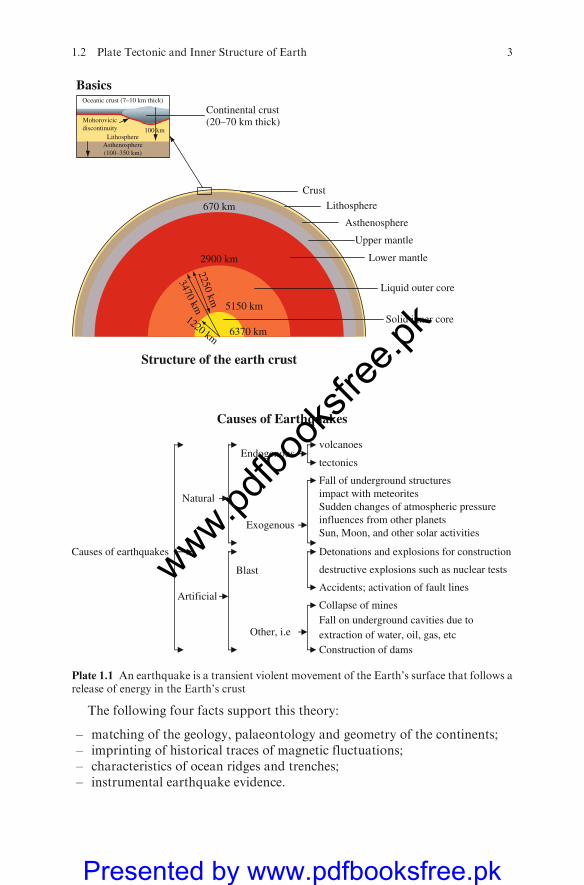
1.2 Plate Tectonic and Inner Structure of Earth
The Earth is roughly spherical with an average radius of around 6,400 km. Its
inner structure was determined from the propagation of earthquake waves. TheEarth consists of three spherical shells of quite different physical properties. The
M.Y.H. Bangash, Earthquake Resistant Buildings,DOI 10.1007/978-3-540-93818-7_1, � M.Y.H. Bangash 2011
1
www.pdfbo
oksfr
ee.pk
Presented by www.pdfbooksfree.pk

outer shell is a thin crust of thickness varying from a few kilometres to a few tensof kilometres; the middle shell is the mantle, about 2,900 km thick, and theMoho (Mohorovicic) discontinuity is its interface with the crust; the innermostshell contains the core, of radius approximately 3,500 km. The crust is made ofvarious types of rock, differing in composition and thickness in its oceanic andcontinental parts. The crust in the continental part consists of two layers,granitic in the outer and basaltic in the inner layer, with total thickness about30–40 km, but reaching 70 km under high mountains, such as in the Qing-Zangplateau of west China. The crust under the oceans is basaltic only, with nogranitic deposit, with a thickness of only about 5 km. The mantel consistsmainly of comparatively uniform ultrabasic olivine rock; its outer 40–70 kmshell together with the crust is usually referred to as the lithosphere, directlyunder which is a layer of soft viscoelastic asthenosphere a few hundreds ofkilometres in thickness. The wave velocity in the asthenosphere is obviouslylower than those in its neighbouring rocks, perhaps due to its viscoelastic, orcreep, property under high temperature and confining pressure. The lithosphereand asthenosphere together form the upper mantle. Below, the lower mantleextends a further 1,900 km or so. The core consists of outer and inner cores.Because it is found that no transverse wave can propagate through the outercore, it is agreed that the outer core is in a liquid state.
Temperature increases from crust to core. The temperature is about 6008Cat adepth of 20km, 1,000–1,5008C at 100 km, 2,0008C at 700 km and 4,000–5,0008Cin the core. The high temperature comes from the heat release from radioactivematerial inside the Earth. The distributions of the radioactive material underocean or under the continents may be different, and this is considered to be thecause of current movement of materials in the mantle.
Pressure increases also from crust to core, perhaps 89.676 KN/cm2 in theupper mantle, 139.49 KN/cm2 in the outer core and 36,867 KN/cm2 in the innercore.
Plate tectonics was developed on the hypothesis of sea-floor spreading dur-ing the past few decades. According to this concept, the rigid lithosphere,consisting of six major plates, drifts on the rheological asthenosphere, like aship on the ocean, but with a very slow speed. The six plates are the Eurasian,Pacific, American, African, Indian and Antarctic. Each plate may then besubdivided into smaller plates. The relative movements of the plates are roughlya few centimetres per year and has continued for at least 200 million years. Thetheory can be described as follows: (1)Material flows out from the uppermantelthrough the lithosphere at ocean ridges where the crust is thin and pushes thelithosphere, whose thickness is a few kilometres, (2) drifting horizontally on theasthenosphere, which shows rheological properties under high temperature,high pressure and permanent horizontal pushing. When two tectonic platescollide, one thrusts under the other and comes back to the lithosphere, whichforms a deep ocean trench and subduction zone at the junction of two plates andvolcanoes and mountains on the plate which remains on the Earth’s surface.A reference is made to the basics given in Plates 1.1, 1.2 and 1.3.
2 1 Introduction to Earthquake with Explanatory Data
www.pdfbo
oksfr
ee.pk
Presented by www.pdfbooksfree.pk
The following four facts support this theory:
– matching of the geology, palaeontology and geometry of the continents;– imprinting of historical traces of magnetic fluctuations;– characteristics of ocean ridges and trenches;– instrumental earthquake evidence.
Basics
Structure of the earth crust
Causes of Earthquakes
volcanoesEndogenous
tectonics
Fall of underground structures
Natural impact with meteorites Sudden changes of atmospheric pressure
Exogenous influences from other planetsSun, Moon, and other solar activities
Causes of earthquakes Detonations and explosions for construction
Blast destructive explosions such as nuclear tests
Accidents; activation of fault lines Artificial
Collapse of mines Fall on underground cavities due to
Other, i.e extraction of water, oil, gas, etcConstruction of dams
670 km
Upper mantle
Asthenosphere
Lithosphere
Crust
Lower mantle
Liquid outer core
Solid inner core
2900 km
5150 km1220 km
2250 km
3470 km
6370 km
Continental crust(20–70 km thick)
Oceanic crust (7–10 km thick)
Mohorovicicdiscontinuity
LithosphereAsthenosphere(100–350 km)
100 km
Plate 1.1 An earthquake is a transient violent movement of the Earth’s surface that follows arelease of energy in the Earth’s crust
1.2 Plate Tectonic and Inner Structure of Earth 3
www.pdfbo
oksfr
ee.pk
Presented by www.pdfbooksfree.pk
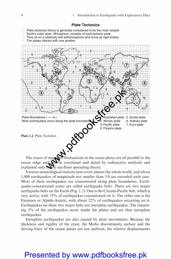
The traces of magnetic fluctuations in the ocean plates are all parallel to the
ocean ridge and can be correlated and dated by radioactive methods and
explained only by the sea-floor spreading theory.Various seismological stations now cover almost the whole world, and about
1,000 earthquakes of magnitude not smaller than 5.0 are recorded each year.
Most of these earthquakes are concentrated along plate boundaries. Earth-
quake-concentrated zones are called earthquake belts. There are two major
earthquake belts on the Earth (Fig. 1.2). One is the Circum-Pacific belt, which is
very active, with 75% of earthquakes concentrated on it. The other one is the
Eurasian or Alpide-Asiatic, with about 22% of earthquakes occurring on it.
Earthquakes on these two major belts are interplate earthquakes. The remain-
ing 3% of the earthquakes occur inside the plates and are thus intraplate
earthquakes.Intraplate earthquakes are also caused by plate movements. Because the
thickness and rigidity of the crust, the Moho discontinuity surface and the
driving force of the ocean plates are not uniform, the relative displacements
Plate Boundaries ( )Most earthquakes occur along the plate boundaries
1. Australian plate2. African plate3. Pacific plate4. Filopino plate
5. Scotia plate6. Arabian plate7. Euro plate
Plate Tectonics- Plate tectonics theory is generally considered to be the most reliable- Earth’s outer layer- lithosphere- consists of hard tectonic plate- They sit on a relatively soft asthenosphere and move as rigid bodies- The plates interact with one another
3
2 6
5
7
1
4
5
6
5
4
4
4
441
4
51
6
1
1
542
2 2
2
2
5
51
1
1
4
55
5
66
45
1
66
61
6
1
55
6
65
4
Plate 1.2 Plate Tectonics
4 1 Introduction to Earthquake with Explanatory Data
www.pdfbo
oksfr
ee.pk
Presented by www.pdfbooksfree.pk
and velocities between plates vary both in space and in time. A plate is usually
under complex stress condition; one part may be under tension, causing depres-
sion, and the other part under compression, causing mountain uplift, or under
shear, causing horizontal deformation.
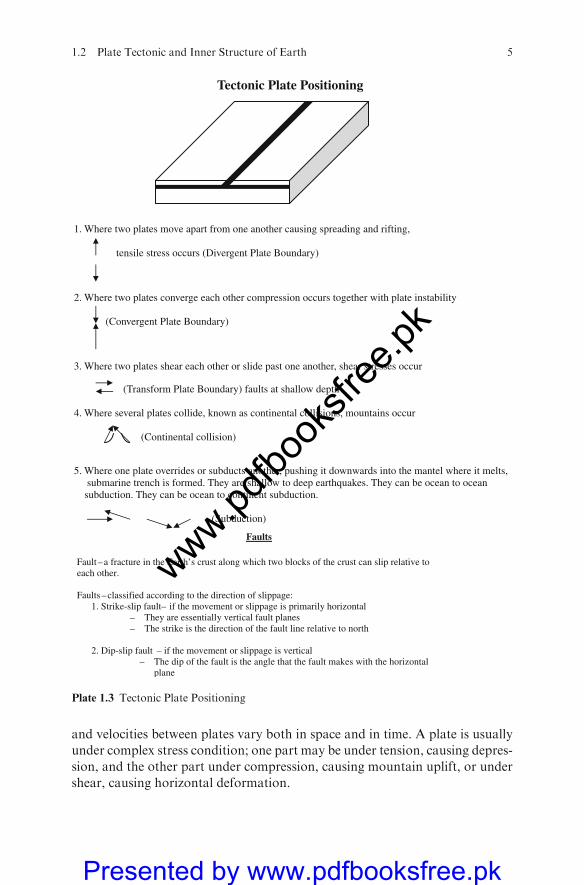
Tectonic Plate Positioning
1. Where two plates move apart from one another causing spreading and rifting,
tensile stress occurs (Divergent Plate Boundary)
2. Where two plates converge each other compression occurs together with plate instability
(Convergent Plate Boundary)
3. Where two plates shear each other or slide past one another, shear stresses occur
(Transform Plate Boundary) faults at shallow depth
4. Where several plates collide, known as continental collisions, mountains occur
(Continental collision)
5. Where one plate overrides or subducts another, pushing it downwards into the mantel where it melts, submarine trench is formed. They are shallow to deep earthquakes. They can be ocean to ocean
subduction. They can be ocean to continent subduction.
)noitcudbuS(
Faults
Fault – a fracture in the Earth’s crust along which two blocks of the crust can slip relative to each other.
Faults – classified according to the direction of slippage:1. Strike-slip fault– if the movement or slippage is primarily horizontal
– They are essentially vertical fault planes– The strike is the direction of the fault line relative to north
2. Dip-slip fault – if the movement or slippage is vertical– The dip of the fault is the angle that the fault makes with the horizontal
plane
Plate 1.3 Tectonic Plate Positioning
1.2 Plate Tectonic and Inner Structure of Earth 5
www.pdfbo
oksfr
ee.pk
Presented by www.pdfbooksfree.pk

Compared with interplate earthquakes, continental earthquakes have thefollowing three features:
a. They are less frequent and less concentrated.b. They are more dangerous to humans.c. The source mechanism varies and is more complicated.
Because the continental plate remains on the Earth’s surface and is ofvarying thickness, it is full of faults and folds under long-term tectonic action,and earthquakes occur with much more scattering.
Deformationdue toplate tectonics is a very slowbut persistingprocess. In a verylong timeperiod, deformationaccumulates elastic strain in the crust.Crustmaterialmay be elastic somewhere but rheologic in other places. If the crust is elastic, strainenergymay be accumulated and itmay crack suddenly when the strength of rock isovercomeand the accumulated energy is transferred into earthquakewaves, and anearthquake occurs. This is the elastic rebound theory of earthquakes.
The rigidity and brittleness of rocks are higher in the crust, and the rockbehaves like an elastic and brittle material.When stress or strain is over the limitcapacity, the rock breaks and the stress drops suddenly from its maximum s0 attime t0 instantly to a minimum value smin. This value can recover to some othervalue of s in between at time t1.
1.3 Types of Faults
Faults may range in length from less than a metre to many hundreds of kilo-metres. In the field, geologists commonly find many discontinuities in rockstructures, which they interpret as faults, and these are drawn on geologicalmaps as continuous or broken lines. The presence of such faults indicates that,at some time in the past, movements took place along them. One now knows thatsuch movement can be either slow slip, which produces no ground shaking, orsudden rupture, which results in perceptible vibrations – an earthquake. Forexample, one of the most famous examples of sudden faults rupture is the SanAndreas Fault in April 1906. However, the observed surface faulting of mostshallow focus earthquakes ismuch shorter in length and showsmuch less offset inthis case. In fact, in the majority of earthquakes, fault rupture does not reach thesurface and is thus not directly visible. The faults seen at the surface sometimesextend to considerable depths in the outermost shell of the Earth, called the crust.This rocky skin, from 5 to 60 km thick, forms the outer part of the lithosphere.
It must be emphasized that slip no longer occurs at most faults plotted ongeological maps. The last displacement to occur along a typical fault may havetaken place tens of thousands or even millions of years ago. The local disruptiveforces in the Earth nearby may have subsided long ago, and chemical processesinvolving water movement may have cemented the ruptures, particularly atshallow depths. Such an inactive fault is now not the site of earthquakes andmay never be again.
6 1 Introduction to Earthquake with Explanatory Data
www.pdfbo
oksfr
ee.pk
Presented by www.pdfbooksfree.pk

The primary interest is of course in active faults, along which crustal displace-ments can be expected to occur. Many of these faults are in rather well-definedtectonically active regions of the Earth, such as themid-oceanic ridges and youngmountain ranges. However, sudden fault displacements can also occur awayfrom regions of clear present tectonic activity.
Whether on land or beneath the oceans, fault displacements can be classifiedinto three types. The plane of the fault cuts the horizontal surface of the groundalong a line whose direction from the north is called the strike of the fault. Thefault plane itself is usually not vertical but dips at an angle down into the Earth.When the rock on that side of the fault hanging over the fracture slips down-wards, below the other side, we have a normal fault. The dip of a normal faultmay vary from 08 to 908. When, however, the hanging wall of the fault movesupwards in relation to the bottom or footwall, the fault is called a reverse fault.A special type of reverse fault is a thrust fault in which the dip of the fault issmall. The faulting in mid-oceanic ridge earthquakes is predominantly normal,whereas mountainous zones are the sites of mainly thrust-type earthquakes.
Both normal and reverse faults produce vertical displacements – seen at thesurface as fault scarps – called dip-slip faults. By contrast, faulting that causesonly horizontal displacements along the strike of the fault is called transcurrentor strike-slip. It is useful in this type to have a simple term that tells the directionof slip. For example, the arrows on the strike-slip fault show a motion that iscalled left-lateral faulting. It is easy to determine if the horizontal faulting is left-lateral or right-lateral. Imagine that one is standing on one side of the fault andlooking across it. If the offset of the other side is from right to left, the faulting isleft-lateral, whereas if it is from left to right, the faulting is right-lateral. Ofcourse, sometimes faulting can be a mixture of dip-slip and strike-slip motion.
In an earthquake, serious damage can arise not only from the groundshaking but also from the fault displacement itself, although this particularearthquake hazard is very limited in area. It can usually be avoided by thesimple expedient of obtaining geological advice on the location of active faultsbefore construction is undertaken. These concepts are clearly indicated in theworld conferences on Earthquake Engineering, mostly held in CaliforniaInstitute of Technology, California.
1.4 Seismograph And Seismicity
Seismicity is a description of the relationship of time, space, strength andfrequency of earthquake occurrence within a certain region and its under-standing is the foundation of earthquake study. Since there is still no practicalway to control earthquakes, one can only try to understand and follow theirnature wisely to prepare for possible strong earthquakes through prediction,earthquake engineering and society or governmental efforts of disasterreduction.
1.4 Seismograph And Seismicity 7
www.pdfbo
oksfr
ee.pk
Presented by www.pdfbooksfree.pk
The most popular way to study seismicity is empirically or statistically.A seismic belt is defined first to have a similar past earthquake distributionand geological and tectonic background, with dimensions somewhat similar tothe ones already familiar.
Although earthquake-recording instruments, called seismographs, are nowmore sophisticated, the basic principle employed is the same. A mass on a freelymovable support can be used to detect both vertical and horizontal shaking of theground. The vertical motion can be recorded by attaching the mass to a springhanging from an anchored instrument frame; the bobbing of the frame (as with akitchen scale) will produce relative motion. When the supporting frame is shakenby earthquake waves, the inertia of the mass causes it to lag behind the motion ofthe frame, and this relative motion can be recorded as a wiggly line by pen and inkon paper wrapped around a rotating drum (alternatively the motion is recordedphotographically or electromagnetically on magnetic tape or as discrete digitalsamples for direct computer input). For measurements of the sideways motion ofthe ground, the mass is usually attached to a horizontal pendulum, which swingslike a door on its hinges. Earthquake records are called seismograms. A seismo-graph appears to be no more than a complicated series of wavy lines, but fromthese lines a seismologist can determine the hypocentre location, magnitude andsource properties of an earthquake. Although experience is essential in interpret-ing seismograms, the first step in understanding the lines is to remember thefollowing principles. First, earthquake waves consist predominantly of threetypes – P-waves and S-waves, which travel through the Earth, and a third type,surface waves, which travel around the Earth. If you look closely enough, you willfind that almost always each kind of wave is present on a seismogram, particularlyif it is recorded by a sensitive seismograph at a considerable distance from theearthquake source. Each wave type affects the pendulums in a predetermined way.Second, the arrival of a seismic wave produces certain telltale changes on theseismogram trace: The trace is written more slowly or rapidly than just before;there is an increase in amplitude; and the wave rhythm (frequency) changes. Third,from past experience with similar patterns, the reader of the seismogram canidentify the pattern of arrivals of the various phases.
A common time standard must be used to compare the arrival times ofseismic waves between earthquake observatories around the world. Tradition-ally, seismograms are marked in terms of Universal Time (UT) or GreenwichMean Time (GMT), not local time. The time of occurrence of an earthquake inUT can easily be converted to local time, but be sure to make allowance forDaylight Saving Time when this is in effect.
1.5 Seismic Waves
Human understanding of earthquakes, and of other physical sciences, comes firstfrom macroseismic phenomena, but ultimately from instrumental observation.It is the instrumental data for seismic waves that provide quantitative
8 1 Introduction to Earthquake with Explanatory Data
www.pdfbo
oksfr
ee.pk
Presented by www.pdfbooksfree.pk

understanding of the earthquake source mechanism and of the interior construc-tion of the Earth. Although the Earth’s materials show rheological propertiesunder static forces from plate tectonic movement, they show elastic propertiesunder the dynamic action of seismic waves from earthquakes; the weak viscosityunder dynamic forces can be considered in terms of energy-absorbing dampingadded to the elastic properties.
Nowadays, for the great majority of earthquakes, the location is determinedfrom the time taken by P seismic waves (and sometimes S-waves) to travel fromthe focus to a seismograph. Many hundreds of modern seismographs areoperated worldwide continuously and reliably for this and other purposes. Insome seismic areas, special local networks of seismographic stations have beeninstalled to locate the foci of even very small earthquakes.
Today, almost everyone is familiar with the concept of digital signals ratherthan continuous recordings, the latter provided by the continually varyingelectric currents that drove the old-style pen-and-ink (or even magnetic tape)recording seismographs. New technology allows modern seismographs torecord the continuous ground motions as a finely spaced series of separatenumbers; such discrete numerical sampling is defined by the binary number or‘‘bits’’. This form makes the recordings, unlike analog seismograms, immedi-ately accessible for computer processing. In the 1970s, seismologists beganto take full advantage of this emerging digital technology; now it iscommonplace.
The first global project of any size to convert globally distributed seismo-graphs began in the 1970s. The digital samples had 14 bits. This numberprovided the dynamic range of frequencies that spanned what is called a broad-band seismographic system – that is, from periods of a fraction of a second tothe periods of free vibrations of the Earth (approximately 1 h) – and even out tothe tidal deformations of the Earth (days). The intensity of shaking is observedto vary greatly with the direction around a fault rupture. The physical reason isthat the seismic source is a moving energy emitter – like the whistle on a movingtrain. The energy increases as the source approaches and decreases as it movesaway. A simple comparison of seismograms from the 1992 Landers, California,earthquake has been plotted. The shaking is represented as ground acceleration,velocity and displacement.
1.6 Magnitude of the Earthquake
The first known seismic instrument, the Houfeng seismometer, made in the yearAD 132 in the Late Han dynasty by the ancient Chinese scientist Heng Zhang,successfully recorded an earthquake inAD 138. Themodern type of seismographstarted in the eighteenth century and includes three subsystems: sensor, amplifierand recorder. For the special requirements of the seismologist, the seismographrecords usually the displacement of the ground motion due to an earthquake.
1.6 Magnitude of the Earthquake 9
www.pdfbo
oksfr
ee.pk
Presented by www.pdfbooksfree.pk
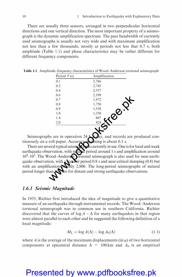
There are usually three sensors, arranged in two perpendicular horizontal
directions and one vertical direction. The most important property of a seismo-
graph is the dynamic amplification spectrum. The pass bandwidth of currently
used seismographs is usually not very wide and with maximum amplification
not less than a few thousands, mostly at periods not less that 0.7 s; both
amplitude (Table 1.1) and phase characteristics may be rather different for
different frequency components.
Seismographs are in operation 24 h a day, and records are produced con-tinuously on a roll paper. Accuracy of timing is about 0.1 s.
There are several typical seismographs currently in use.One is for local andweakearthquake observation, with natural period around 1 s and amplification around104–105. The Wood–Anderson torsional seismograph is also used for near-earth-quake observation, with a natural period 0.8 s and near-critical damping (0.8) butwith an amplification of only 2,800. The long-period seismographs of naturalperiod longer than 10 s are for distant and strong earthquake observations.
1.6.1 Seismic Magnitude
In 1935, Richter first introduced the idea of magnitude to give a quantitativemeasure of an earthquake through instrumental records. The Wood–Andersontorsional seismograph was in common use in southern California. Richterdiscovered that the curves of logA� D for many earthquakes in that regionwere almost parallel to each other and he suggested the following definition of alocal magnitude:
ML ¼ logAðDÞ � logA0ðDÞ (1:1)
where A is the average of the maximum displacements (in m) of two horizontalcomponents at epicentral distance D = 100 km and A0 is an empirical
Table 1.1 Amplitude–frequency characteristics of Wood–Anderson torsional seismograph
Period T (s) Amplification
0.1 2,786
0.2 2,745
0.4 2,557
0.6 2,199
0.7 1,972
0.8 1,750
0.9 1,538
1.0 1,350
1.4 807
2.0 424
10 1 Introduction to Earthquake with Explanatory Data
www.pdfbo
oksfr
ee.pk
Presented by www.pdfbooksfree.pk
correction for the effect of local conditions on attenuation of ground motion.As shown in Table 1.1, the amplification at period T = 1.0 s drops to abouthalf of that of T=0.1 s; this definition is therefore made for magnitude on thebasis of short-period ground motion and is adequate for local smallearthquakes.
Since seismic stations are not normally so densely allocated as in southernCalifornia, Gutenberg followed the same idea and defined a surface wavemagnitude for shallow and distant earthquakes as follows:
Ms ¼ logAðDÞ � logA0ðDÞ (1:2)
At a distance of about 2,000 km, the primary wave is a surface wave of periodabout 20 s; A is defined as the maximum vector of the horizontal displacementin m of a 20 s period wave.
SinceMs cannot be used for deep earthquakes, he defined the following bodywave magnitude:
mb ¼ logðA=TÞmax �QðD; hÞ (1:3)
where (A/T)max may be themaximum ratio ðA=TÞ of P, PP or S waves, either thevertical or horizontal vector displacement in m, and T in seconds is the periodcorresponding toA. But in practice, most seismographs have a natural period of1 s and A of the vertical component is used to define the body wave.
Empirical conversion relations have been suggested between these magni-tudes, such as
Ms ¼ 1:59mb � 40 ¼ 1:27ðML � 1:0Þ � 0:16M2L (1:4)
In China, when these definitions are used, the correction term logA0 orQðD; hÞincludes also the instrument correction; the conversion relation used is
Ms ¼ 1:13ML � 1:08 (1:5)
1.7 The World Earthquake Countries and Codes of Practices
A reference is made to the Author’s book on ‘‘Proto type Building Structures’’(Thomas Telford, London) for many details. Table 1.2 and 1.3 give the list ofcountries with lethal earthquakes with average return periods. The statisticsrecording casualties due to earthquake include a wide range of events such asfires, tsunamis generated by offshore events, rockfalls, landslides and otherhazards triggered by earthquakes. Most large-scale disasters given by Table1.4 due to earthquakes result from the collapse of buildings. The number ofsignificant earthquakes can also be viewed in Fig. 1.1.
1.7 The World Earthquake Countries and Codes of Practices 11
www.pdfbo
oksfr
ee.pk
Presented by www.pdfbooksfree.pk

Table 1.2 The world’s earthquake countries
Earthquakeranking
No. of lethalearthquakes1900–2008
Averagereturnperiod(years)
Earthquakeranking
No. of lethalearthquakes1900–2008
Averagereturnperiod(years)
1. China 1958 0.6 40. New Zealand 6 15
2. Japan 201 1 41. Uganda 1 100+
3. Italy 43 2 42. Lebanon 1 100+
4. Iran 135 1 43. Portugal 4 23
5. Turkey 135 1 44. Puerto Rico 1 100+
6. CIS (USSR) 46 2 45. Dominican
7. Peru 53 2 Republic 1 100+
8. Pakistan 248 5 46. Zaire 3 30
9. Chile 34 3 47. Ethiopia 3 30
10. Indonesia 148 2 48. Solomon Islands 2 50
11. Guatemala 14 7 49. Canada 3 30
12. India 221 4 50. Bangladesh 5 18
13. Nicaragua 3 31 51. Panama 2 50
14. Morocco 2 46 52. France 2 50
15. Nepal 14 23 53. Cyprus 2 50
16. Philippines 55 4 54. South Africa 6 15
17. Mexico 71 2 55. Mongolia 1 100+
18. Taiwan 49 2 56. Egypt 13 30
19. Ecuador 26 4 57. Ghana 1 100+
20. Argentina 22 8 58. Tunisia 1 100+
21. Algeria 41 5 59. Australia 2 50
22. Yemen 3 31 60. Malawi 1 100+
23. El Salvador 13 7 61. Cuba 18 50
24. Romania 4 23 62. Haiti 8 50
25. Costa Rica 7 13 63. Spain 15 23
26. Yugoslavia 18 5 64. Bolivia 4 23
27. Colombia 29 3 65. Poland 2 50
28. Afghanistan 41 8 66. Tanzania 2 50
29. USA 32 3 67. Honduras 3 30
30. Greece 51 2 68. Czechoslovakia 1 100+
31. Jamaica 2 50 69. Hungary 2 50
32. Burma 31 9 70. Belgium 1 100+
33. Venezuela 16 6 71. Iceland 1 100+
34. Albania 24 7 72. Germany 1 100+
35. Papua New 73. Israel 12 –
36. Guinea 15 10 74. Burundi 1 –
37. Bulgaria 6 15 75. Iraq 6 –
38. Jordan 2 50 76. Sudan 5 –
39. Libya 2 50 77. Syria 5 –
Note: Data collected by the author from reports, newspapers and television records by the author.
12 1 Introduction to Earthquake with Explanatory Data
www.pdfbo
oksfr
ee.pk
Presented by www.pdfbooksfree.pk

Table 1.3 Major earthquakes: magnitudes and fatalities
Date LocationMagnitude (Richterscale) Fatalities
26 January 2001 India 7.9 >13,000
21 September1999
Taiwan 7.6 2,400
17 August 1999 Western Turkey 7.4 17,000
25 January 1999 Western Colombia 6 1,171
4 February 1998 Northeast Afghanistan 6.1 5,000
10 May 1997 Northern Iran 7.1 1,500
17 January 1995 Kobe, Japan 7.2 >6,000
30 September1993
Latur, India 6.0 >10,000
21 June 1990 Northwest Iran 7.3–7.7 50,000
7 December 1988 Northwest Armenia 6.9 25,000
19 September1985
Central Mexico 8.1 >9,500
16 September1978
Northeast Iran 7.7 25,000
28 July 1976 Tangshan, China 7.8–8.2 755,000
4 February 1976 Guatemala 7.5 22,778
26 December1939
Erzincan province, Turkey 7.9 33,000
24 January 1939 Chillan, Chile 8.3 28,000
1 September 1923 Tokyo-Yokohama, Japan 8.3 200,000
16 December1920
Gansu, China 8.6 100,000
16 August 1906 Valparaiso, Chile 8.6 20,000
18–19 April 1906 San Francisco (CA), USA 7.7–7.9 3,000 andfire
28 December1908
Messina, Italy 7.5 83,000
13 January 1915 Avezzano, Italy 7.5 29,980
22 May 1927 Nan-Shan, China 8.3 200,000
26 December1932
Gansu, China 7.6 70,000
31 May 1935 Quetta, India 7.5 60,000
6 October 1948 Iran/USSR 7.3 100,000
15 August 1950 Assam, India 8.7 1,530
29 February 1960 Agadir, Morocco 5.7 12,000
1 September 1962 Northwestern Iran 7.1 12,000
26 July 1963 Skopje, Yugoslavia 6.0 1,100
27 March 1964 Anchorage (AL), USA 9.2 131
31 August 1968 Northeastern Iran 7.4 11,600
5 January 1970 Yunan Province, China 7.7 10,000
31 May 1970 Chimbote, Peru 7.8 67,000
23 December1972
Managua, Nicaragua 6.2 5,000
6 May 1976 Friuli, Italy 6.5 939
Note: Data from reports, newspapers and T.V. records by the author.
1.7 The World Earthquake Countries and Codes of Practices 13
www.pdfbo
oksfr
ee.pk
Presented by www.pdfbooksfree.pk

Table 1.3 (continued)
Date LocationMagnitude (Richterscale) Fatalities
4 March 1977 Romania 7.5 1,541
10 October 1980 Northern Algeria 7.7 3,000
23 November1980
Southern Italy 7.2 4,800
13 December1982
Northern Yemen 6.0 1,600
17 October 1989 San Francisco (CA), USA 7.1 62
16 July 1990 Luzon, Philippines 7.7 1,660
29 September1993
Maharashtra, India 6.3 9,800
13–16 October1993
Papua New Guinea 6.8 >60
6 June 1994 Cauca, Colombia 6.8 1,000
16 January 1995 Kobe, Japan 7.2 5,500
14 June 1995 Sakhalin Island, Russia 7.6 2,000
28 February 1997 Baluchistan Province,Pakistan
7.3 >100
7 September 1999 Athens, Greece 5.9 125
26 December2003
Bam, Iran 6.6 30,000
8 October 2005 Kashmir, Pakistan 8.5 >76,000
23 January 2005 Sulawesi, Indonesia 6.2 1
25 January 2005 Turkey/Iraq Border 5.9 2
2 February 2005 Jara, Indonesia 4.8 1
5 February 2005 Celebes Sea 7.1 2
22 February 2005 Central Iran 6.4 612
9 March 2005 South Africa 5.0 2
20 March 2005 Kyushu, Japan 6.6 1
28 March 2005 Northern Sumatra 8.7 1,313
12 December2005
Hindu Kush, Afghanistan 6.5 5
14 December2005
Uttaranchal, India 5.3 1
1 April 2006 Taiwan 6.2 >42
4 April 2006 Pakistan, N.W.F.P 4.7 >28
14 April 2006 Norwegiansca 3.3 –
20 April 2006 Koryakia, Russia 7.6 40
25 April 2006 Tasmania, Australia 2.2 4
29 April 2006 Koryakia, Russia 6.6 –
30 April 2006 Atacama, Chile 6.7 –
30 April 2006 Atacama, Chile 6.5 –
3 May 2006 Tonga 7.9 –
7 May 2007 Central Iran 4.8 –
16 May 2006 Kermadec Islands 7.4 –
16 May 2006 Nias, Indonesia 6.8 –
22 May 2006 Koryakia, Russia 6.6 –
Note: Data collected and tabulated from reports, newspapers and T.V. records by the author.
14 1 Introduction to Earthquake with Explanatory Data
www.pdfbo
oksfr
ee.pk
Presented by www.pdfbooksfree.pk

Table 1.3 (continued)
Date LocationMagnitude (Richterscale) Fatalities
15 Jan 2010 Haiti 7.2 >100,000
23 May 2006 Anglesev 1.5 –
26 May 2006 Java, Indonesia 6.3 5,749
28 May 2006 Papua New Guinea 6.5 –
3 June 2006 Southern Iran 5.4 2
8 June 2006 Shieldaig 2.9 –
11 June 2006 Kyushhu, Japan 6.3 –
13 June 2006 Albania 4.5 –
20 June 2006 Gansu, China 5.1 –
28 June 2006 Southern Iran 5.8 9
14 May 2008 China 7.9 50,000
Note: Data Collected from various reports, newspapers and television records by the author.
Table 1.4 Locations of large-scale earthquakes: types, magnitudes and fatalities
Date Location Magnitude Fatalities Comments
23 January 1556 Shansi, China 8 830,000 –
26 December 2004 Sumatra 9.1 283,106 Deaths fromearthquake andtsunami
27 July 1976 Tangshan, China 7.5 255,000 Estimated deathtoll as high as655,000
9 August 1138 Aleppo, Syria 230,000
22 December 856 Damghan, Iran 200,000
22 May 1927 Tsinghai, China 7.9 200,000 Large fractures
16 December 1920 Gansu, China 7.8 200,000 Major fractures,landslides
23 March 893 Ardabil, Iran 150,000
1 September 1923 Kanto (Kwanto),Japan
7.9 143,000 Great Tokyo fire
5 October 1948 USSR(Turkmenistan,Ashgabat)
7.3 110,000
28 December 1908 Messina, Italy 7.2 70,000 –100,000(estimated)
Deaths fromearthquake andtsunami
September 1290 Chihli, China 100,000
8 October 2005 Pakistan 7.6 80,361
November 1667 Shemakha,Caucasia
80,000
18 November1727
Tabriz, Iran 77,000
25 December 1932 Gansu, China 7.6 70,000
1 November 1755 Lisbon, Portugal 8.7 70,000 Great tsunami
31 May 1970Haiti
Peru–
7.97.1
66,000>100,000
$530,000,000damage, greatslide, floods
Note: Data from various reports by the author.
1.7 The World Earthquake Countries and Codes of Practices 15
www.pdfbo
oksfr
ee.pk
Presented by www.pdfbooksfree.pk

Table 1.4 (continued)
Date Location Magnitude Fatalities Comments
30 May 1935 Quetta, Pakistan 7.5 30,000 –60,000
Quetta almostcompletelydestroyed
11 January 1693 Sicily, Italy 60,000
1268 Silicia, Asia Minor 60,000
20 June 1990 Western Iran 7.7 40,000 –50,000
Landslides
4 February 1783 Calabria, Italy 50,000
19 April 1902 Guatemala 14 N91 W
7.5 2,000 –
16 December 1902 Turkestan 40.8 N72.6 E
6.4 4,500 –
19 April 1903 Turkey 39.1 N42.4 E
1,700
28 April 1903 Turkey 39.1 N42.5 E
6.3 2,200 –
4 April 1905 Kangra, India33.0 N 76.0 E
7.5 19,000 –
8 September 1905 Calabria, Italy39.4 N 16.4 E
7.9 2,500 –
31 January 1906 Colombia-Ecuador1 N 81.5 W
8.8 1,000 –
16 March 1906 Formosa, Kagi(Taiwan) 23.6 N120.5 E
7.1 1,300 –
18 April 1906 San Francisco,California 38.0 N123.0 W
7.8 about 3,000 Deaths fromearthquake andfire
17 August 1906 Valparaiso, Chile 33S 72 W
8.2 20,000 –
14 January 1907 Kingston, Jamaica18.2 N 76.7 W
6.5 1,600 –
21 October 1907 Central Asia 38 N69 E
8.1 12,000 –
28 December 1908 Messina, Italy 38 N15.5 E
7.2 70,000 –100,000(estimated)
Deaths fromearthquake andtsunami
23 January 1909 Iran 33.4 N 49.1 E 7.3 5,500 –
9 August 1912 Marmara Sea40.5 N 27 E
7.8 1950 –
13 January 1915 Avezzano, Italy42 N 13.5 E
7.5 29,980 –
21 January 1917 Bali, Indonesia 8.0 S115.4 E
15,000 –
30 July 1917 China 28.0 N104.0 E
6.5 1,800 –
13 February 1918 Kwangtung(Guangdong),China 23.5 N117.0 E
7.3 10,000 –
Note: Data collected and tabulated from reports, newspapers and T.V. records by the author.
16 1 Introduction to Earthquake with Explanatory Data
www.pdfbo
oksfr
ee.pk
Presented by www.pdfbooksfree.pk

Table 1.4 (continued)
Date Location Magnitude Fatalities Comments
16 December 1920 Gansu, China35.8 N 105.7 E
7.8 200,000 Major fractures,landslides
24 March 1923 China 31.3 N100.8 E
7.3 5,000 –
25 May 1923 Iran 35.3 N 59.2 E 5.7 2,200 –
1 September 1923 Kanto (Kwanto),Japan 35.0 N139.5 E
7.9 143,000 Great Tokyo fire
16 March 1925 Yunnan, China25.5 N 100.3 E
7.1 5,000 Talifu almostcompletelydestroyed
7 March 1927 Tango, Japan35.8 N 134.8 E
7.6 3,020 –
22 May 1927 Tsinghai, China36.8 N 102.8 E
7.9 200,000 Large fractures
1 May 1929 Iran 38 N 58 E 7.4 3,300 –
6 May 1930 Iran 38.0 N 44.5 E 7.2 2,500 –
23 July 1930 Italy 41.1 N 15.4 E 6.5 1,430 –
31 March 1931 Nicaragua 13.2 N85.7 W
5.6 2,400 –
25 December 1932 Gansu, China39.7 N 97.0 E
7.6 70,000 –
2 March 1933 Sanriku, Japan39.0 N 143.0 E
8.4 2,990 –
25 August 1933 China 32.0 N103.7 E
7.4 10,000 –
15 January 1934 Bihar-Nepal, India26.6 N 86.8 E
8.1 10,700 –
20 April 1935 Formosa 24.0 N121.0 E
7.1 3,280 –
30 May 1935 Quetta, Pakistan29.6 N 66.5 E
7.5 30,000 –60,000
Quetta almostcompletelydestroyed
16 July 1935 Taiwan 24.4 N120.7 E
6.5 2,700 –
25 January 1939 Chillan, Chile 36.2 S72.2 W
7.8 28,000 –
26 December 1939 Erzincan, Turkey39.6 N 38 E
7.8 30,000 –
10 November1940
Romania 45.8 N26.8 E
7.3 1,000 –
26 November1942
Turkey 40.5 N34.0 E
7.6 4,000 –
20 December 1942 Erbaa, Turkey40.9 N 36.5 E
7.3 3,000 Some reports of1,000 killed
10 September1943
Tottori, Japan35.6 N 134.2 E
7.4 1,190 –
1.7 The World Earthquake Countries and Codes of Practices 17
www.pdfbo
oksfr
ee.pk
Presented by www.pdfbooksfree.pk

Table 1.4 (continued)
Date Location Magnitude Fatalities Comments
26 November1943
Turkey 41.0 N33.7 E
7.6 4,000 –
15 January 1944 San Juan, Argentina31.6 S 68.5 W
7.8 5,000 Reports of asmany as 8,000killed
1 February 1944 Turkey 41.4 N32.7 E
7.4 2,800 Reports of asmany as 5,000killed
7 December 1944 Tonankai, Japan33.7 N 136.2 E
8.1 1,000 –
12 January 1945 Mikawa, Japan34.8 N 137.0 E
7.1 1,900 –
27 November1945
Iran 25.0 N 60.5 E 8.2 4,000 –
31 May 1946 Turkey 39.5 N41.5 E
6.0 1,300 –
10 November1946
Ancash, Peru 8.3 S77.8 W
7.3 1,400 Landslides, greatdestruction
20 December 1946 Tonankai, Japan32.5 N 134.5 E
8.1 1,330 –
28 June 1948 Fukui, Japan 36.1 N136.2 E
7.3 5,390 –
5 October 1948 USSR(Turkmenistan,Ashgabat) 38.0 N58.3 E
7.3 110,000 –
5 August 1949 Ambato, Ecuador1.2 S 78.5 E
6.8 6,000 Large landslides,topographicalchanges
15 August 1950 India, Assam–Tibet28.7 N 96.6 E
8.6 1,530 Greattopographicalchanges,landslides,floods
18 March 1953 Western Turkey40.0 N 27.5 E
7.3 1,103 Yenice destroyedand majordamages atGonen and Can.Felt throughoutthe AegeanIslands andsouthernGreece.Microseismicarea estimatedat 2,000 squaremiles. Damageestimated about$3,570,000.
18 1 Introduction to Earthquake with Explanatory Data
www.pdfbo
oksfr
ee.pk
Presented by www.pdfbooksfree.pk

Table 1.4 (continued)
Date Location Magnitude Fatalities Comments
9 September 1954 Orleansville, Algeria36 N 1.6 E
6.8 1,250 –
27 June 1957 USSR (Russia)56.3 N 116.5 E
1,200 –
2 July 1957 Iran 36.2 N 52.7 E 7.4 1,200 –
13 December 1957 Iran 34.4 N 47.6 E 7.3 1,130 –
29 February 1960 Agadir, Morocco30 N 9 W
5.7 10,000 –15,000
Occurred atshallow depth
22 May 1960 Chile 39.5 S 74.5 W 9.5 4,000 – 5,000 Tsunami, volcanicactivity, floods
1 September 1962 Qazvin, Iran 35.6 N49.9 E
7.3 12,230 –
26 July 1963 Skopje, Yugoslavia42.1 N 21.4 E
6.0 1,100 Occurred atshallow depthjust undefined
19 August 1966 Varto, Turkey,39.2 N 41.7 E
7.1 2,520 –
31 August 1968 Iran 34.0 N 59.0 E 7.3 12,000 –20,000
–
25 July 1969 Eastern China21.6 N 111.9 E
5.9 3,000 –
4 January 1970 Yunnan Province,China 24.1 N102.5 E
7.5 10,000 –
28 March 1970 Gediz, Turkey39.2 N 29.5 E
6.9 1,100 –
31 May 1970 Peru 9.2 S 78.8 W 7.9 66,000 $530,000,000damage, greatrock floods
22 May 1971 Turkey 38.83 N40.52 E
6.9 1,000 –
10 April 1972 Southern Iran28.4 N 52.8 E
7.1 5,054 –
23 December 1972 Managua,Nicaragua 12.4 N86.1 W
6.2 5,000 –
10 May 1974 China 28.2 N104.0 E
6.8 20,000 –
28 December 1974 Pakistan 35.0 N72.8 E
6.2 5,300 –
4 February 1975 China 40.6 N122.5 E
7.0 10,000 –
6 September 1975 Turkey 38.5 N40.7 E
6.7 2,300 –
4 February 1976 Guatemala 15.3 N89.1 W
7.5 23,000 –
6 May 1976 Northeastern Italy46.4 N 13.3 E
6.5 1,000 –
1.7 The World Earthquake Countries and Codes of Practices 19
www.pdfbo
oksfr
ee.pk
Presented by www.pdfbooksfree.pk

Table 1.4 (continued)
Date Location Magnitude Fatalities Comments
25 June 1976 West Irian (NewGuinea) 4.6 S140.1 E
7.1 422 5,000 – 9,000missing andpresumed dead
27 July 1976 Tangshan, China39.6 N 118.0 E
7.5 255,000(official)
Estimated deathtoll as high as650,000
16 August 1976 Mindanao,Philippines 6.3 N124.0 E
7.9 8,000 –
24 November1976
NorthwestIran–USSRborder 39.1 N44.0 E
7.3 5,000 Deaths estimated
4 March 1977 Romania 45.8 N26.8 E
7.2 1,500 –
16 September1978
Iran 33.2 N 57.4 E 7.8 15,000 –
10 October 1980 El Asnam (formerlyOrleansville),Algeria 36.1 N1.4 E
7.7 3,500 –
23 November1980
Southern Italy40.9 N 15.3 E
7.2 3,000 –
11 June 1981 Southern Iran29.9 N 57.7 E
6.9 3,000 –
28 July 1981 Southern Iran30.0 N 57.8 E
7.3 1,500 –
13 December 1982 Western ArabianPeninsula 14.7 N44.4 E
6.0 2,800 –
30 October 1983 Turkey 40.3 N42.2 3 E
6.9 1,342 –
19 September1985
Michoacan, Mexico18.2 N 102.5 W
8.0 9,500(official)
Estimated deathtoll as high as30,000
10 October 1986 El Salvador 13.8 N89.2 W
5.5 1,000 –
6 March 1987 Colombia–Ecuador0.2 N 77.8 W
7.0 1,000 –
20 August 1988 Nepal–India borderregion 26.8 N86.6 E
6.8 1,450 –
7 December 1988 Spitak, Armenia41.0 N 44.2 E
6.8 25,000 –
20 June 1990 Western Iran 37.0 N49.4 E
7.7 40,000 –50,000
Landslides
16 July 1990 Luzon, PhilippineIslands 15.7 N121.2 E
7.8 1,621 Landslides,subsidence andsand.
20 1 Introduction to Earthquake with Explanatory Data
www.pdfbo
oksfr
ee.pk
Presented by www.pdfbooksfree.pk

Table 1.4 (continued)
Date Location Magnitude Fatalities Comments
19 October 1991 Northern India30.8 N 78.8 E
7.0 2,000 –
12 December 1992 Flores Region,Indonesia 8.5 S121.9 E
7.5 2,500 Tsunami raninland 300 m,water height25 m
29 September1993
Latur-Killari, India18.1 N 76.5 E
6.2 9,748 –
16 January 1995 Kobe, Japan 34.6 N135 E
6.9 5,502 Landslide,liquefaction
27 May 1995 Sakhalin Island52.6 N 142.8 E
7.5 1,989 –
10 May 1997 Northern Iran33.9 N 59.7 E
7.5 1,560 4,460 injured,60,000 homeless
4 February 1998 Tajikistan BorderRegion-Afghanistan37.1 N 70.1 E
6.1 2,323 818 injured, 8,094housesdestroyed
30 May 1998 Tajikistan borderregion–Afghanistan37.1 N 70.1 E
6.9 4,000 At least 4,000people killed,many thousandsinjured andhomeless inBadakhshanand Takharprovince inAfghanistan
17 July 1998 Papua New Guinea2.96 S 141.9 E
7.0 2,183 Thousandsinjured, about9,500 homelessand about 500missing as aresult of tsunamiwith maximumwave heightestimated at10 m
25 January 1999 Colombia 4.46 N75.82 W
6.2 1,185 Over 700 missingand presumedkilled. Over4,750 injuredand about250,000homeless
17 August 1999 Turkey 40.7 N30.0 E
7.6 17,118 At least 50,000injured,thousandshomeless.Damageestimated at3 billion USD
1.7 The World Earthquake Countries and Codes of Practices 21
www.pdfbo
oksfr
ee.pk
Presented by www.pdfbooksfree.pk
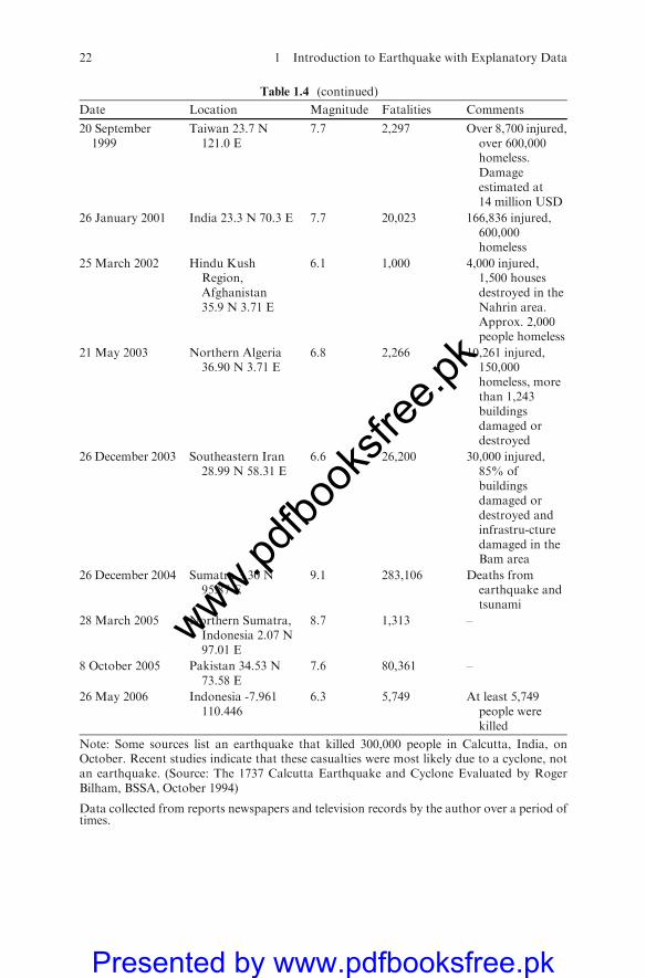
Table 1.4 (continued)
Date Location Magnitude Fatalities Comments
20 September1999
Taiwan 23.7 N121.0 E
7.7 2,297 Over 8,700 injured,over 600,000homeless.Damageestimated at14 million USD
26 January 2001 India 23.3 N 70.3 E 7.7 20,023 166,836 injured,600,000homeless
25 March 2002 Hindu KushRegion,Afghanistan35.9 N 3.71 E
6.1 1,000 4,000 injured,1,500 housesdestroyed in theNahrin area.Approx. 2,000people homeless
21 May 2003 Northern Algeria36.90 N 3.71 E
6.8 2,266 10,261 injured,150,000homeless, morethan 1,243buildingsdamaged ordestroyed
26 December 2003 Southeastern Iran28.99 N 58.31 E
6.6 26,200 30,000 injured,85% ofbuildingsdamaged ordestroyed andinfrastru-cturedamaged in theBam area
26 December 2004 Sumatra 3.30 N95.87 E
9.1 283,106 Deaths fromearthquake andtsunami
28 March 2005 Northern Sumatra,Indonesia 2.07 N97.01 E
8.7 1,313 –
8 October 2005 Pakistan 34.53 N73.58 E
7.6 80,361 –
26 May 2006 Indonesia -7.961110.446
6.3 5,749 At least 5,749people werekilled
Note: Some sources list an earthquake that killed 300,000 people in Calcutta, India, onOctober. Recent studies indicate that these casualties were most likely due to a cyclone, notan earthquake. (Source: The 1737 Calcutta Earthquake and Cyclone Evaluated by RogerBilham, BSSA, October 1994)
Data collected from reports newspapers and television records by the author over a period oftimes.
22 1 Introduction to Earthquake with Explanatory Data
www.pdfbo
oksfr
ee.pk
Presented by www.pdfbooksfree.pk

1.8 Intensity Scale
The word ‘‘intensity’’ may be defined qualitatively as ‘‘the quality or condition
of being intense’’ or quantitatively as ‘‘magnitude, as of energy or a force per
unit of area or time’’. The term earthquake intensity was introduced to be a
physical quantity, but through qualitative or fuzzy definitions. In the earth-
quake engineering field, some consider it a qualitative rating through the
intensity scale, but many engineers consider it an equivalent of ground peak
acceleration intensity.There are three properties of earthquake intensity defined by macroseismic
phenomena:
1. A composite measure of multiple scales: intensity is defined through thelevels of human response, structural damage, changes in natural phenom-ena and behaviour of objects during or after an earthquake. Each of thesefour responses is a scale, and intensity ratings are specified in each scale.When the measurements of each individual scale differ from each other as
Fig. 1.1 Seismicity of the world (courtesy of Cartographic Data Atlas version 1.02, BritishGeological Survey Worldwide Earthquake Database)(Ref. Prototype Building Structures, Thomas Telford, London 1993.)
1.8 Intensity Scale 23
www.pdfbo
oksfr
ee.pk
Presented by www.pdfbooksfree.pk
usually happens, a subjective decision is made, such as in China, byindividuals who rate the intensity, but the maximum rating is taken inEurope.
2. A ranking and fuzzy measure through macroseismic description: on eachindividual scale, the scaling is not quantitative but qualitative in terms offuzzy ranks, such as a ‘‘few’’, ‘‘some’’, ‘‘many’’, ‘‘most’’, for the number ofitems considered; ‘‘slight’’, ‘‘moderate’’, ‘‘heavy’’, ‘‘serious’’, for strength ofresponse. These are typical fuzzy set terms, i.e. they are defined throughqualitative description, and the boundaries between ranks are not clear butfuzzy.
3. Indirectness of defining a cause through the results if intensity means groundmotion: many building design codes still define intensity as ground motion. Itis quite clear that ground motion is the cause of its effects on objects. Therelation between cause and effects must be rough or fuzzy if the objects, as wellas the cause and effects, are not clearly defined as in the case of an intensityscale.
The term earthquake intensity has been used for more than 170 years before
the term earthquake magnitude and is still widely used. Its usage includes the
following three aspects:
4. As a simple measure of earthquake damage: after a strong earthquake,government and society want to know the general level of damage and itsdistribution in order to take emergency action. It is relatively easy to estimateafter an earthquake and to be understood by ordinary people, just like windintensity.
5. As a simple macroseismic scale for the strength of earthquake motionfor the seismologist: historical earthquake data are damage data, whichhave been used to study past seismicity. Without damage data, thehistory of earthquakes would cover only a few decades, too short toknow the spatial and temporal distribution of earthquakes or theirseismicity.
6. As a rough but convenient index to sum up experience to earthquakeengineering construction and to depict zones of seismic hazard(Hu, C1983): many countries use intensity as index for zonation,such as Russia, China and several European countries, and manycountries have previously used it, such as the United States, Canadaand India.
1.8.1 Earthquake Intensity Scale
The macroseismic idea of earthquake intensity was a natural product 170 years
ago when no instruments were available to measure any physical quantity of
ground motion and the requirement of earthquake description was also simple,
24 1 Introduction to Earthquake with Explanatory Data
www.pdfbo
oksfr
ee.pk
Presented by www.pdfbooksfree.pk
just a scale or a single number or grade to describe its strength or magnitude.
The earliest record of earthquake intensity may be traced back to 1564 inEurope. When discussing the effect of an earthquake, different colours are
used to show different effects on a map. Up to the nineteenth century, thereappeared many earthquake intensity scales, mostly used to grade the localdamage or effect. During the early period, macroseismic phenomena were the
only means possible to define the indices of the intensity scale. As an example,the one commonly used is the abridgedModifiedMercalli (MM) intensity scale,from which a general and brief idea of intensity may be obtained. A reference is
made to Tables 1.1, 1.2, 1.3, 1.4, 1.5, 1.6 and 1.7.An effective earthquake-resisting design for buildings in an area subject to
seismic activity depends on the characteristics of earthquakes, namely fre-quency content, intensity and duration. The type of construction, soil condi-
tions and a number of other complex factors concerning dynamic modelling,load–structure– soil interactions, etc. are additional areas which need to beinvestigated.
The genealogy of the intensity scales is described in a step-by-step manner inFigs. 1.1 and 1.2. The most well-known intensity scales, Modified Mercalli
(Richter) and Medvedev–Sponheuer–Karnik (MSK), are fully described inTables 1.3, 1.4 and 1.5. These tables are needed to assess the damage to
structures such as buildings and their components. A guide to earthquakemagnitude is given in Tables 1.3, 1.4, 1.5, 1.6 and 1.7.
1.8.2 Intensity Distribution
1.8.2.1 Isoseismal Map
The intensity contour or isoseismal map is a simple way to show the general
damage to a strong earthquake on a map. After field investigations an isoseis-mal map is drawn in the following two stages:
1. The original intensity ratings of all sites investigated are indicated on adetailed map.
2. Contour lines of equal intensities are drawn which group sites of the sameintensity in the same zone.
For the design of buildings three approaches are specified and are givenbelow:
(a) Seismic coefficient method: Various codes recommend this method. Flex-ibility or stiffness methods are employed. Specified shear distribution ascubic parabola in various building storeys is recommended. This approachis adopted for buildings no more than 40 m high.
(b) Modal analysis: Modal analysis using average acceleration spectra and amultiplying factor is adopted for buildings within the range of 40–90m height.
1.8 Intensity Scale 25
www.pdfbo
oksfr
ee.pk
Presented by www.pdfbooksfree.pk

Table 1.5 Modified Mercalli intensity scale
I. Not felt except by a very few under exceptionally favourable circumstances.
II. Felt by persons at rest, on upper floors, or favourably placed.
III. Felt indoors; hanging objects swing; vibration similar to passing of light trucks;duration may be estimated; may not be recognized as an earthquake.
IV. Hanging objects swing; vibration similar to passing of light trucks; or sensation of ajolt similar to a heavy ball striking the walls; standing motor cars rock; windows,dishes and doors rattle; glasses clink and crockery clashes; in the upper range of IVwooden walls and frames creak.
V. Felt outdoors; direction may be estimated; sleepers wakened, liquids disturbed, somespilled; small unstable objects displaced or upset; doors swing, close or open;shutters and pictures move; pendulum clocks stop, start or change rate.
VI. Felt by all; many frightened and run outdoors; walking unsteady; windows, dishesand glassware broken; knick-knacks, books, etc., fall from shelves and picturesfrom walls; furniture moved or overturned; weak plaster and masonry D* cracked;small bells ring (church or school); trees and bushes shaken (visibly, or heard torustle).
VII. Difficult to stand; noticed by drivers of motor cars; hanging objects quiver; furniturebroken; damage to masonry D, including cracks; weak chimneys broken at roofline; fall of plaster, loose bricks, stones, tiles, cornices (also unbraced parapets andarchitectural ornaments); some cracks in masonry C*; waves on ponds; waterturbid with mud; small slides and caving in along sand or gravel banks; large bellsring; concrete irrigation ditches damaged.
VIII. Steering of motor cars affected; damage to masonry C or partial collapse; somedamage to masonry B*; none to masonry A*; fall of stucco and some masonrywalls; twisting and fall of chimneys, factory stacks, monuments, towers andelevated tanks; frame housesmoved on foundations if not bolted down; loose panelwalls thrown out; decayed piling broken off; branches broken from trees; changesin flow or temperature of springs and wells; cracks in wet ground and on steepslopes.
IX. General panic; masonry D destroyed; masonry C heavily damaged, sometimes withcomplete collapse; masonry B seriously damaged; general damage to foundations;frame structures if not bolted shifted off foundations; frames racked; seriousdamage to reservoirs; underground pipes broken; conspicuous cracks in ground; inalluviated areas sand and mud ejected, earthquake fountains and sand cratersappear.
X. Most masonry and frame structures destroyed with their foundations; some well-builtwooden structures and bridges destroyed; serious damage to dams, dykes andembankments; large landslides; water thrown on banks of canals, rivers, lakes, etc.;sand and mud shifted horizontally on beaches and flat land; rails bent slightly.
XI. Rails bent greatly; underground pipelines completely out of service.
XII. Damage nearly total; large rock masses displaced; lines of sight and level distorted;objects thrown into the air.
Masonry A: Good workmanship, mortar and design; reinforced, especially laterally, andbound together by using steel, concrete, etc., designed to resist lateral forces.
Masonry B: Good workmanship and mortar; reinforced but not designed in detail to resistlateral forces.
Masonry C: Ordinary workmanship and mortar; no extreme weaknesses like failing to tie inat corners, but neither reinforced nor designed against horizontal forces.
Masonry D: Weak materials, such as adobe; poor mortar; low standards of workmanship;weak horizontally.
26 1 Introduction to Earthquake with Explanatory Data
www.pdfbo
oksfr
ee.pk
Presented by www.pdfbooksfree.pk

Table 1.6 Seismic intensity scale MSK-81 Medvedev–Sponheuer–Karnik 1981 Revision
Intensity degree I: Not noticeable
The intensity of the vibration is below the limit of sensibility; the tremor is detected andrecorded by seismographs only.
Intensity degree II: Scarcely noticeable (very slight)
Vibration is felt only by individual people at rest in houses, especially on upper floors ofbuildings.
Intensity degree III: Weak
The earthquake is felt indoors by a few people, outdoors only in favourable circumstances.The vibration is weak. Attentive observers notice a slight swinging of hanging objects,somewhat more heavily on upper floors.
Intensity degree IV: Largely observed
The earthquake is felt indoors by many people, outdoors by a few. Here and there people areawakened, but no one is frightened. The vibration is moderate. Windows, doors and dishesrattle. Floors and walls creak. Furnitures begin to shake. Hanging objects swing slightly.Liquids in open vessels are slightly disturbed. In standing motor cars the shock is noticeable.
Intensity degree V: Strong
Effects on people and surroundings: The earthquake is felt indoors by most, outdoors bymany. Many sleeping people are awakened. A few run outdoors. Animals become uneasy.Buildings tremble throughout. Hanging objects swing considerably. Pictures swing out ofplace. Occasionally pendulum clocks stop. Unstable objects may be overturned or shifted.Open doors and windows are thrust open and slam back again. Liquids spill in smallamounts from well-filled open containers. The vibration is strong, resembling sometimesthe fall of a heavy object in the building.
Effects on structures: Damage of grade 1 in a few buildings of type A is possible.
Effects on nature: Sometimes change in flow of springs.
Intensity degree VI: Slight damage
Effects on people and surroundings: Felt by most indoors and outdoors. Many people inbuildings are frightened and run outdoors. A few persons lose their balance. Domesticanimals run out of their stall. In a few instances dishes and glassware may break. Books falldown. Heavy furniture may possibly move and small steeple bells may ring.
Effects on structures: Damage of grade 1 is sustained in single buildings of type B and in manyof type A. Damage in few buildings of type A is of grade 2.
Effects on nature: In a few cases cracks up to widths of 1 cm are possible in wet ground; inmountains occasional landslips; changes in flow of springs and in level of well water areobserved.
Intensity degree VII: Damage to buildings
Effects on people and surroundings: Most people are frightened and run outdoors. Many findit difficult to stand. Persons driving motor cars notice the vibration. Large bells ring.
Effects on structures: In many buildings of type C damage of grade 1 is caused; in manybuildings of type B damage is of grade 2.Many buildings of type A suffer damage of grade 3,a few of grade 4. In some instances landslips of roadway on steep slopes occur; local cracks inroads and stonewalls.
Effects on nature: Waves are formed on water, and water is made turbid by mud stirred up.Water levels in wells change, and the flow of springs changes. In a few cases dry springs havetheir flow restored and existing springs stop flowing. In isolated instances parts of sandy orgravelly banks slip off.
Intensity degree VIII: Destruction of buildings
Effects on people and surroundings: General fright; a few people show panic, also personsdriving motor cars are disturbed. Here and there branches of trees break off. Even heavyfurniture moves and partly overturns. Hanging lamps are in part damaged.
1.8 Intensity Scale 27
www.pdfbo
oksfr
ee.pk
Presented by www.pdfbooksfree.pk

Table 1.6 (continued)
Effects on structures: Many buildings of type C suffer damage of grade 2 and a few of grade 3.Many buildings of type B suffer damage of grade 3 and a few of grade 4. Many buildings oftype A suffer damage of grade 4 and a few of grade 5.Memorials andmonuments move andtwist. Tombstones overturn. Stone walls collapse.
Effects on nature: Small landslips on hollows and on banked roads on steep slopes; cracks inground up to widths of several centimetres. New reservoirs come into existence. Sometimesdry wells refill and existing wells become dry. In many cases change in flow and level ofwater or wells.
Intensity degree IX: General damage to buildings
Effects on people and surroundings: General panic; considerable damage to furniture.Animals run to and fro in confusion and cry.
Effects on structures: Many buildings of type C suffer damage of grade 3 and a few of grade 4.Many buildings of type B show damage of grade 4, a few of grade 5. Many buildings oftype A suffer damage of grade 5. Monuments and columns fall. Reservoirs may showheavy damage. In individual cases railway lines are bent and roadways damaged.
Effects on nature: On flat land overflow of water, sand and mud is often observed. Groundcracks to widths of up to 10 cm, in slopes and river banks more than 10 cm; furthermore, alarge number of slight cracks in ground; falls of rock, many landslides and earth flows; largewaves on water.
Intensity degree X: General destruction of buildings
Effects on structures: Many buildings of type C suffer damage of grade 4, a few of grade 5.Many buildings of type B show damage of grade 5, most of type A collapse. Dams, dykesand bridges may show severe to critical damage. Railway lines are bent slightly. Roadpavements and asphalt show wary folds.
Effects on nature: In ground, cracks up to widths of several decimetres, sometimes up to 1 m.Broad fissures occur parallel to water courses. Loose ground slides from steep slopes.Considerable landslides are possible from river banks and steep coast. In coastal areasdisplacement of sand and mud; water from canals, lakes, river, etc., thrown on land. Newlakes occur.
Intensity degree XI: Catastrophe
Effects on structures: Destruction of most and collapse of many buildings of type C. Evenwell-built bridges and dams may be destroyed and railway lines largely bent, thrusted orbucked; highways become unusable; underground pipes destroyed.
Effects on nature: Ground fractured considerably by broad cracks and fissures, as well as bymovement in horizontal and vertical directions; numerous landslides and fall of rocks. Theintensity of the earthquake requires to be investigated especially.
Intensity degree XII: Landscape changes
Effects on structures: Practically all structures above and below ground are heavily damagedor destroyed.
Effects on nature: The surface of the ground is radically changed. Considerable groundcracks with extensive vertical and horizontal movement are observed. Fall of rocksand slumping of river banks over wide areas; lakes are dammed; waterfalls appear,and rivers are deflected. The intensity of the earthquake requires to be investigatedespecially.
Type of structures (building not antiseismic)
A Buildings of fieldstone, rural structures, adobe houses, clay houses.B Ordinary brick buildings, large block construction, half-timbered structures, structures of
hewn blocks of stone.C Precast concrete skeleton construction, precast large panel construction, well-built
wooden structures.
28 1 Introduction to Earthquake with Explanatory Data
www.pdfbo
oksfr
ee.pk
Presented by www.pdfbooksfree.pk

Table 1.6 (continued)
Classification of damage to buildings
Grade 1: Slight damage: fine cracks in plaster; fall of small pieces of plaster.Grade 2: Moderate damage: small cracks in walls; fall of fairly large pieces of plaster; pantiles
slip off; cracks in chimneys; parts of chimneys fall down.Grade 3: Heavy damage: large and deep cracks in walls; fall of chimneys.Grade 4: Destruction: gaps in walls; parts of buildings may collapse; separate parts of the
buildings lose their cohesion; inner walls and filled-in walls of the frame collapse.Grade 5: Total damage: total collapse of buildings.
Table 1.7 A guide to earthquake magnitude
Magnitudes less than 4.5
Magnitude 4.5 represents an energy release of about 108 kJ and is the equivalent of about 10 tof TNT being exploded underground. Below about magnitude 4.5, it is extremely rare foran earthquake to cause damage, although it may be quite widely felt. Earthquakes ofmagnitude 3 and magnitude 2 become increasingly difficult for seismographs to detectunless they are close to the event. A shallow earthquake of magnitude 4.5 can generally befelt for 50–100 km from the epicentre.
Magnitude 4.5–5.5 – local earthquakes
Magnitude 5.5 represents an energy release of around 109 kJ and is the equivalent of about100 t of TNT being exploded underground. Earthquakes of magnitude 5.0–5.5 may causedamage if they are shallow and if they cause significant intensity of ground shaking in areasof weaker buildings. Earthquakes up to magnitude of about 5.5 can occur almost anywherein the world – this is the level of energy release that is possible in normal non-tectonicgeological processes such as weathering and land formation. An earthquake of magnitude5.5 may well be felt 100–200 km away.
Magnitude 6.0–7.0 – large magnitude events
Magnitude 6 represents an energy release of the order of 1010 kJ and is the equivalent ofexploding about 6,000 t of TNT underground. Amagnitude 6.3 is generally taken as beingabout equivalent to an atomic bomb being exploded underground. A magnitude 7.0represents an energy release of 1012 kJ. Large magnitude earthquakes of magnitude 6.0and above are much larger energy releases associated with tectonic processes. If theyoccur close to the surface they may cause intensities at their centre of VIII, IX or even X,causing very heavy damage or destruction if there are towns or villages close to theirepicentre. Some of these large magnitude earthquakes, however, are associated withtectonic processes at depth and may be relatively harmless to people on the Earth’ssurface. There are about 200 large magnitude events somewhere in the world each decade.A magnitude 7.0 earthquake at shallow depth may be felt at distances 500 km or morefrom its epicentre.
Magnitudes 7.0–8.9 – great earthquakes
A magnitude 8 earthquake releases around 1013 kJ of energy, equivalent to more than 400atomic bombs being exploded underground, or almost as much as a hydrogen bomb. Thelargest earthquake yet recorded, magnitude 8.9, released 1014 kJ of energy. Greatearthquakes are themassive energy releases caused by long lengths of linear faults rupturingin on break. If they occur at shallow depths they cause slightly stronger epicentral intensitiesthan large magnitude earthquakes but their great destructive potential is due to the verylarge areas that are affected by strong intensities.
1.8 Intensity Scale 29
www.pdfbo
oksfr
ee.pk
Presented by www.pdfbooksfree.pk
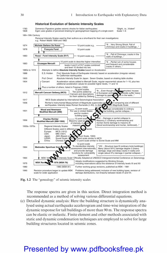
The response spectra are given in this section. Direct integration method isrecommended as a method of solving various differential equations.
(c) Detailed dynamic analysis: Here the building structure is dynamically ana-lysed using actual earthquake accelerogram and time-wise integration of thedynamic response for tall buildings of more than 90m. The response spectracan be elastic or inelastic. Finite element and other methods associated withstatic and dynamic condensation techniques are employed to solve for largebuilding structures located in seismic zones.
Historical Evolution of Seismic Intensity ScalesDomenico Pignatoro grades seismic shocks for Italian earthquakes:Egen uses grades of perceived shaking for geolographical mapping of a single event
Personal Intensity Scales used by their authors as a shorthand for their own investigationse.g. Robert Mallet 1858 and 1862
10 point scale e.g..
10 point scale
10 point scale e.g..
E.S. Holden First ‘Absolute Scale of Earthquake Intensity’ based on acceleration (irregular values)for Californian earthquakes
Prof. Omori Absolute Intensity Scale for Japan: Seven Grades, based on shaking table studies
Cancani
Plus a number of others, listed in Freeman (1930)12 point scales
Two points added byCancani and descriptionsfor them added by Seiberg
MCS Scale adopted by international Seismological AssociationRichter’s Instrumental Measurement of Magnitude supercodes intensity for comparing size of differentearthquakes. Intensity takes Roman Numerals (I–XII), to distinguish from Magnitude Scale
“VIII: ...Damage considerable to ordinarysubstantial building, partial collapse...”
12 point scaleFor use in United States
and for modernbuilding types12 point scale
Masonry used as indicatorof intensity. 4 grades of
masonry proposed
“VIII: ...Damage or partial collapse toMasonry C (Ordinary workmanship andmortar) Some damage to masonry B(Good workmanship and mortar, reinforced)...”Regional Intensity Scales
Different Scales used in different areas of the world:Europe: MCS (1912)USA: MM (1931)Japan: JMA (Based on 7 point Omori Scale, 1900)USSR: Soviet Scale (1931) 12 point scale similar to MCSChina: Chinese Scale (1956) 12 point scale similar to Soviet Scale and MM
Medvedev Sponhuer Karnik (MSK)
MSK ‘International Intensity Scale’ Officially Adopted at UNESCO Intergovernmental Conference on Seismology
Adopts modifications suggested by Working Groups,including reservations about the existence of intensity levels XI and XII
Further working group revisions, published as MSK - 1981
Problems being addressed; inclusion of new building types, revision ofdamage distributions, non-linearity between levels VI and VII.
Revision procedure began to update MSKscale for wider application
MSK Revisions 1976 (MSK-76)
1964
1930s–1970s
1956
1931
19361917
1912
1904
1900
1888
1880s to 1915
1883
1883
1878
1874
18th–19th Century
17831828
1964
1976
1980
1990
12 point scaleTo standardise intensity
assessment internationallyand provide damage
functions for vulnerabilityassessment
“VIII: ...Structure type B (ordinary brick buildings)Many (about 50%) damage degree 3 (heavydamage, large and deep cracks in walls) andsingle (about 5%) damage 4 (partial collapse)...”
“8: ...Even though solidly constructed, housesof European architecture generally suffer heavydamage by gaping fissures in the walls...”
“8: ...Very Strong Shock. Fall ofchimneys and cracks in buildings...”
“Slight...to...Violent”Scale 1–6
“8: ...Fall of Chimneys, cracks in thewalls of buildings...”
Acceleration values added to Mercalli Scale, regular exponential values for 1–10, plus twoadditional acceleration values for possible higher levels, 11 and 12
Attempts to define Absolute Intensity Scales based on Acceleration
levels 4 and 5 of R-F scales combinedand level 10 divided into two
Michele Stefano De Rossi
François Forel
Rossi - Forel Intensity Scale (R-F)
Giuseppe Mercalli
Mercalli Cancani Seiberg (MCS)
Wood and NewmannModified Mercalli (MM)
Charles RichterModified Mercalli (MM-1956)
1980 (MSK-81)
“8: ...Partial ruin of some housesand frequent and considerablecracks in others...”
10 point scale to describe higher intensities
Fig. 1.2 The ‘‘genealogy’’ of seismic intensity scales
30 1 Introduction to Earthquake with Explanatory Data
www.pdfbo
oksfr
ee.pk
Presented by www.pdfbooksfree.pk
A greater detail of such methods is given in Part B of the book, Methods ofAnalysis, and in the Appendix.
Design for drift and lateral stability is important and should be addressed inthe early stages of the building design development. The concept of lateralstability and its relationship to drift and the P� D effect has been codified. Inan earthquake area the relative displacement of buildings is measured by anoverall drift ratio or index. This ratio is either of the following:
(i) the ratio of the relative displacement of a particular floor to the storey heightat that level;
(ii) relative displacement between two adjacent floors.
The drift index is the drift divided by the storey height.Stability analysis sections and the Appendix provide details for drift, lateral
stability and P� D. The limitations of these are given by various codes.Because of the wide scattering of data, judgement is necessary for the second
stage. The routine compromise is to have one set of isoseismals starting from theepicentral area with the highest intensity and decreasing outwards by a decre-ment of one grade with fairly smooth contours and some individual contoursscattered almost randomly. The former is considered to represent the generalintensity distribution, which reflects attenuation of damage away from theepicentre, and the latter as abnormal intensity areas, which reflect the localvariations of site conditions and other effects.
If intensity is rated by the highest indication of an intensity scale, theisoseismals will be the envelope of intensity scale; as the Chinese do, theisoseismals will be some average.
1.8.3 Abnormal Intensity Region
Since site conditions over a wide region change quite often, abnormal intensityareas are actually quite common and can be found in almost any strong earth-quake. In mountainous regions, local topography and soil conditions aremainly responsible; in alluvial plains, soft and weak soils are the major causeof abnormality. There are areas where abnormal intensities have been reportedfor several historical earthquakes. For example, the Yutian area, about 50 kmnorthwest of Tangshan City, was an area of abnormally low intensity in boththe 1679 Sanhe-Pinggu and the 1976 Tangshan earthquakes.
1.8.4 Factors Controlling Intensity Distribution
1.8.4.1 Source Effect
The term ‘‘earthquake source’’ is used here for the whole region where strainenergy is released in the form of earthquake waves during one earthquake.Energy density, geometry of the source and its position in space are the
1.8 Intensity Scale 31
www.pdfbo
oksfr
ee.pk
Presented by www.pdfbooksfree.pk

controlling factors of intensity distribution. The overall shape of isoseismals iscontrolled by the source. For example, small earthquakes have small sourcesand the isoseismals are usually circular; but very large earthquakes have ingeneral extended sources, i.e. with one horizontal dimension much longer thanthe other, and the isoseismals of higher intensities are usually elongated orelliptical. For example, the surface faulting of the 1970 Tonghai earthquakewas about 60 km long and the isoseismals of intensities VII, VIII, IX andXwerevery narrow, with a short-axis/long-axis ratio less than one-third.
1.8.4.2 Distance Effect
The effect of distance is clear and it is the main factor of attenuation. There areseveral definitions of distance and their distinction is important for the nearfield, i.e. the epicentre and the neighbouring areas. The epicentral distancedepends on the definition of epicentre. The instrumental epicentre is the easiestto use with instrumental records, but it has the lowest correlation with intensitydistribution. The fault distance or the shortest distance to the fault is even betterwhen surface faulting can be found.
1.9 Earthquake Intensity Attenuation
The relationship of intensity variation with magnitude and distance is usuallyreferred to as the attenuation law.
1.9.1 Epicentral Intensity and Magnitude
The epicentral intensity I0 was used to represent the size of an earthquake beforethe earthquake magnitude was suggested. Although epicentral intensity alsodepends on focal depth h, it can still be used for a certain specified narrow rangeof focal depth, say 10–30 km, which is the rough average of most strong earth-quakes. To estimate the magnitude of historical earthquakes, the relationbetween epicentral intensity I0 and magnitude M that given by Gutenbergand Richter (1956) for the southern California region is useful.
1.10 Geotechnical Earthquake Engineering
Geotechnical earthquake engineering can be defined as that subspecialty withinthe field of geotechnical engineering which deals with the design and constructionof projects in order to resist the effects of earthquakes. Geotechnical earthquakeengineering requires an understanding of basic geotechnical principles as well asgeology, seismologyand earthquake engineering. In abroad sense, seismologycan
32 1 Introduction to Earthquake with Explanatory Data
www.pdfbo
oksfr
ee.pk
Presented by www.pdfbooksfree.pk
be defined as the study of earthquakes. This would include the internal beheviourof the Earth and the nature of seismic waves generated by the earthquake.
The first step in geotechnical earthquake engineering is often to determinethe dynamic loading from the anticipated earthquake (the anticipated earth-quake is also known as the design earthquake). For the analysis of earthquakes,the types of activities that may need to be performed by the geotechnicalengineer include the following:
– Investigating the possibility of liquefaction at the site. Liquefaction cancause a complete loss of the soil’s shear strength, which could result in abearing capacity failure, excessive settlement or slope movement.
– Calculating the settlement of the structure caused by the anticipatedearthquake.
– Checking the design parameters for the foundation, such as the bearing capa-city andallowable soil bearingpressures, tomake sure that the foundationdoesnot suffer a bearing capacity failure during the anticipated earthquake.
– Investigating the stability of slopes for the additional forces imposed duringthe design earthquake. In addition, the lateral deformation of the slopeduring the anticipated earthquake may need to be calculated.
– Evaluation of the effect of the design earthquake on the stability ofstructures.
– Analysing other possible earthquake effects, such as surface faulting andresonance of the structure.
– Developing site improvement techniques to mitigate the effects of theanticipated earthquake. These include ground stabilization and ground-water control.
– Determining the type of foundation, such as a shallow or deep foundation.– Assisting the structural engineer by investigating the effects of ground
movement due to seismic forces on the structure and by providing designparameters or suitable structural systems to accommodate the anticipateddisplacement.
1.11 Liquefaction
1.11.1 Introduction
The final three sections of this chapter deal with secondary effects, which aredefined as non-tectonic surface processes that are directly related to earthquakeshaking. Examples of secondary effects are liquefaction, earthquake-inducedslope failures and landslides, tsunamis and seiches.
This section deals with liquefaction. The typical subsurface soil condition thatis susceptible to liquefaction is loose sand, which has been newly deposited orplaced, with a groundwater table near ground surface.During an earthquake, thepropagation of shear waves causes the loose sand to contract, resulting in an
1.11 Liquefaction 33
www.pdfbo
oksfr
ee.pk
Presented by www.pdfbooksfree.pk

increase in pore water pressure. Because the seismic shaking occurs so quickly,the cohesionless soil is subjected to an undrained loading. The increase in porewater pressure causes an upward flow of water to the ground surface, where tiemerges in the form of mud spouts or sand boils. The development of high porewater pressures due to the ground shaking and the upward flow of water mayturn the sand into a liquefied condition, which has been termed liquefaction. Forthis state of liquefaction, the effective stress is zero and the individual soil particlesare released from any confinement, as if the soil particles were floating in water.
Because liquefaction typically occurs in soil with a high groundwater table,its effects are most commonly observed in low-lying areas or adjacent rivers,lakes, bays and oceans.
Structures on top of the loose sand deposit that has liquefied during anearthquake can sink or fall over, and buried tanks will float to the surfacewhen the loose sand is liquefied.
After the soil has liquefied, the excess pore water pressure will start todissipate the length of time that the soil will remain in a liquefied state, whichdepends on two main factors: (1) the duration of the seismic shaking from theearthquake and (2) the drainage condition of the liquefied soil. The longer andthe stronger the cyclic shear stress application from earthquake, the longer thestate of liquefaction persists. Likewise, if the liquefied soil is confined by anupper and a lower clay layer, then it will take longer for the excess waterpressures to dissipate by the flow of water from the liquefied soil. After theliquefaction process is complete, the soil will be in a somewhat denser state.
1.11.2 Types of Damage
As previously mentioned, there could also be liquefaction-induced grounddamage, which causes settlement of structures.
There are two main aspects to the ground surface damage:
1. Sand boils: There could be liquefaction-induced ground loss below the struc-tures as the loss of soil through the development of ground surface sand boils.Often liquefaction, and sand boils are observed at ground surface. A row ofsands often develops at the location of cracks or fissures in the ground.
2. Surface fissures: The liquefied soil could also cause the development ofground face fissures which break the overlying soil into blocks that openand close during earthquakes. Note that the liquefied soil actually flowed outof the fissures.
1.12 Earthquake-Induced Settlement
Buildings founded on solid rocks are least likely to experience earth-quake-induced differential settlement. However, buildings on soils couldbe subjected to many different types of earthquake-induced settlement;
34 1 Introduction to Earthquake with Explanatory Data
www.pdfbo
oksfr
ee.pk
Presented by www.pdfbooksfree.pk

where the earthquake-induced settlement exists the following conditions
must be satisfied:
(a) Settlement versus the factor of safety against liquefaction and is acceptable(b) Liquefaction–induced ground damage has been successfully evaluated and
is ok(c) Volumetric compression is satisfied(d) Settlement due to dynamic loads caused by rocking is within permissible
limits given in various codes.
1.13 Bearing Capacity Analyses for Earthquakes
A bearing capacity failure is defined as a foundation failure that occurs when
the shear stresses in the soil exceed the shear strength of the soil. For both static
and seismic cases bearing capacity failures of foundations can be grouped into
three categories:
– General shear strength– Punching shear strength– Local shear strength
1.14 Slope Stability Analysis for Earthquakes
It is necessary to have a shaking threshold that is needed to produce earth-
quake-induced slope movement. The inertia slope stability analysis is prefered
for those materials that retain their shear strength during the earthquake.
Examples of these types of soil and rock are as follows:
(a) Massive crystalline bedrock and sedimentary rock(b) Soils that tend to dilate during seismic shaking: examples are very stiff to
hard clay(c) Soils that have a stress–strain curve that does not exhibit a significant
reduction in shear strength with strains. Earthquake-induced slope move-ment in these soils often takes the form of soil slumps or soil block slides
(d) Clay that has a low sensitivity(e) Soils located above the groundwater table. They have negative pore water
pressure due to capillary action(f) Landslides that have a distinct rupture surface. Cases such as shear
strength along the rupture surface can be equal to the drained residualshear strength
Tables 1.8 and 1.9 give earthquake-induced slope movements in rocks and
soils with appropriate threshold values.
1.14 Slope Stability Analysis for Earthquakes 35
www.pdfbo
oksfr
ee.pk
Presented by www.pdfbooksfree.pk

1.15 Energy Released in an Earthquake
The earthquake magnitude is defined in terms of logarithm of the amplitude ofrecorded seismic wave, and energy of a wave is proportional to the square of itsamplitude. So, there should be no surprise that the magnitude is also related tothe logarithm of the energy. Several equations have been proposed for thisrelationship in the past. An empirical formula worked out by Gutenberg andRichter (1945; Gutenberg, 1956) relates the energy releaseE to the surface wavemagnitude Ms
log10 E ¼ 4:4þ 1:5Ms (1:6)
where E is in Joules. An alternative version of the energy–magnitude relation,suggested by Bath (1966) for magnitudes Ms>5, is
log10 E ¼ 5:24þ 1:44Ms (1:7)
Table 1.8 Earthquake-induced slope movement in rock
Types ofslopemovement Subdivisions Material type
Minimumslopeinclination
Thresholdvalues
Falls Rockfalls Rocks weakly cemented, intenselyfractured or weathered; containconspicuous planes of weaknessdipping out of slope or containboulders in a weak matrix
408 (1.2:1) ML= 4.0
Slides Rock slides Rocks weakly cemented, intenselyfractured or weathered; containconspicuous planes of weaknessdipping out of slope or containboulders in a weak matrix
358 (1.4:1) ML= 4.0
Rock avalanches Rocks
intenselyfracturedandexhibitingone of thefollowing
properties: significantweathering, planes of weaknessdipping out of slope, weakcementation or evidence ofprevious landsliding
258 (2.1:1) ML= 6.0
Rockslumps
Intensely fractured rocks,preexisting rock slump deposits,shale and other rockscontaining layers of weaklycemented or intenselyweathered material
158 (3.7:1) ML= 5.0
Rockblockslides
Rockshaving
conspicuous bedding planes orsimilar planes of weaknessdipping out of slopes
158 (3.7:1) ML= 5.0
Note: Data collected by the author from references to the World Congress on Earthquakesheld at CALTECH, California, U.S.A.
36 1 Introduction to Earthquake with Explanatory Data
www.pdfbo
oksfr
ee.pk
Presented by www.pdfbooksfree.pk
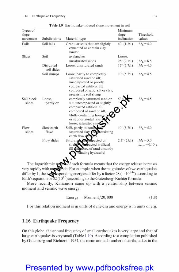
The logarithmic nature of each formula means that the energy release increasesvery rapidlywithmagnitude.For example,when themagnitudesof two earthquakesdiffer by 1, their corresponding energies differ by a factor 28 (=101.44) according toBath’s equation or 32 (101.5) according to theGutenberg–Richter formula.
More recently, Kanamori came up with a relationship between seismicmoment and seismic wave energy:
Energy ¼Moment=20; 000 (1:8)
For this relation moment is in units of dyne-cm and energy is in units of erg.
1.16 Earthquake Frequency
On this globe, the annual frequency of small earthquakes is very large and that oflarge earthquakes is very small (Table 1.10). According to a compilation publishedbyGutenberg andRichter in 1954, themean annual number of earthquakes in the
Table 1.9 Earthquake-induced slope movement in soil
Types ofslopemovement Subdivisions Material type
Minimumslopeinclination
Thresholdvalues
Falls Soil falls Granular soils that are slightlycemented or contain claybinder
408 (1.2:1) ML=4.0
Slides Soil avalanches Loose,
unsaturated sands 258 (2.1:1) ML=6.5
Disruptedsoil slides
Loose, unsaturated sands 158 (3.7:1) ML=4.0
Soil slumps Loose, partly to completelysaturated sand or silt;uncompacted or poorlycompacted artificial fillcomposed of sand, silt or clay,preexisting soil slump
108 (5.7:1) ML=4.5
Soil blockslides
Loose,partly or
completely saturated sand orsilt; uncompacted or slightlycompacted artificial fillcomposed of sand or silt,bluffs containing horizontalor subhorizontal layers ofloose, saturated sand or silt
58 (11:1) ML=4.5
Flowslides
Slow earthflows
Stiff, partly to completelysaturated clay and preexistingearth flow deposits
108 (5.7:1) ML=5.0
Flow slides Saturated, uncompacted orslightly compacted artificialfill composed of sand or sandysilt (including hydraulic)
2.38 (25:1) ML=5.0amax=0.10 g
1.16 Earthquake Frequency 37
www.pdfbo
oksfr
ee.pk
Presented by www.pdfbooksfree.pk
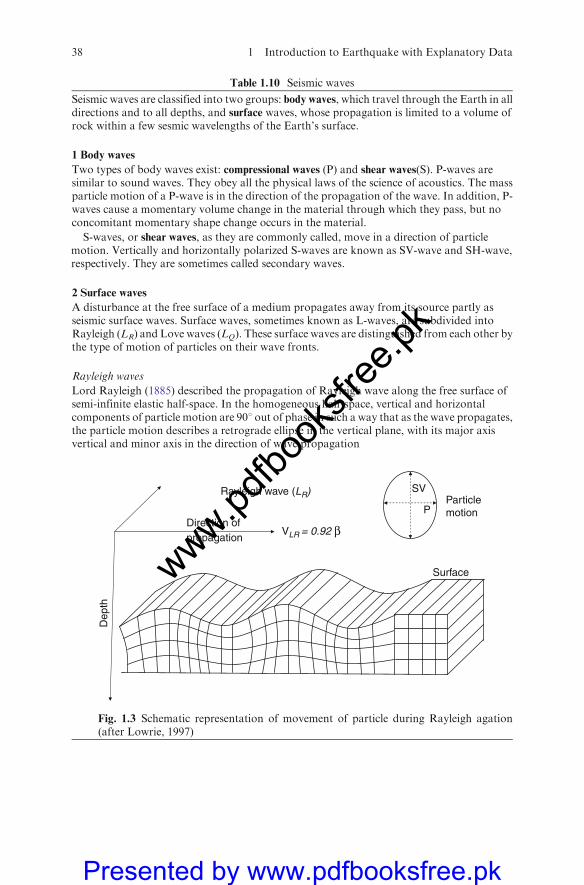
Table 1.10 Seismic waves
Seismic waves are classified into two groups: body waves, which travel through the Earth in alldirections and to all depths, and surface waves, whose propagation is limited to a volume ofrock within a few sesmic wavelengths of the Earth’s surface.
1 Body waves
Two types of body waves exist: compressional waves (P) and shear waves(S). P-waves aresimilar to sound waves. They obey all the physical laws of the science of acoustics. The massparticle motion of a P-wave is in the direction of the propagation of the wave. In addition, P-waves cause a momentary volume change in the material through which they pass, but noconcomitant momentary shape change occurs in the material.
S-waves, or shear waves, as they are commonly called, move in a direction of particlemotion. Vertically and horizontally polarized S-waves are known as SV-wave and SH-wave,respectively. They are sometimes called secondary waves.
2 Surface waves
A disturbance at the free surface of a medium propagates away from its source partly asseismic surface waves. Surface waves, sometimes known as L-waves, are subdivided intoRayleigh (LR) and Love waves (LQ). These surface waves are distinguished from each other bythe type of motion of particles on their wave fronts.
Rayleigh waves
Lord Rayleigh (1885) described the propagation of Rayleigh wave along the free surface ofsemi-infinite elastic half-space. In the homogeneous half-space, vertical and horizontalcomponents of particle motion are 908 out of phase in such a way that as the wave propagates,the particle motion describes a retrograde ellipse in the vertical plane, with its major axisvertical and minor axis in the direction of wave propagation
Direction of propagation
Rayleigh wave (LR)
VLR = 0.92 β
Surface
Particlemotion
SV
P
Dep
th
Fig. 1.3 Schematic representation of movement of particle during Rayleigh agation(after Lowrie, 1997)
38 1 Introduction to Earthquake with Explanatory Data
www.pdfbo
oksfr
ee.pk
Presented by www.pdfbooksfree.pk
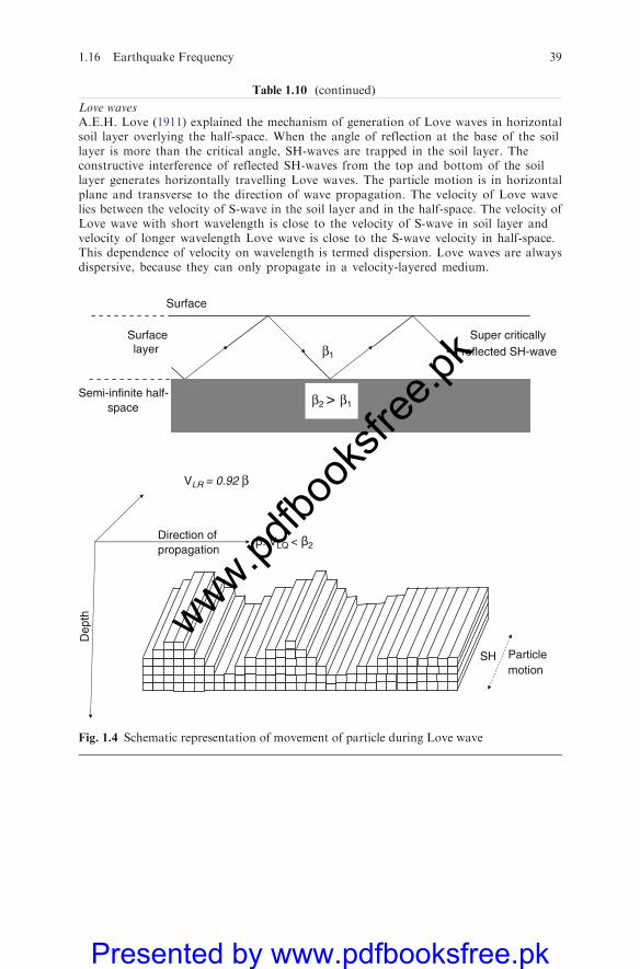
Table 1.10 (continued)
Love wavesA.E.H. Love (1911) explained the mechanism of generation of Love waves in horizontalsoil layer overlying the half-space. When the angle of reflection at the base of the soillayer is more than the critical angle, SH-waves are trapped in the soil layer. Theconstructive interference of reflected SH-waves from the top and bottom of the soillayer generates horizontally travelling Love waves. The particle motion is in horizontalplane and transverse to the direction of wave propagation. The velocity of Love wavelies between the velocity of S-wave in the soil layer and in the half-space. The velocity ofLove wave with short wavelength is close to the velocity of S-wave in soil layer andvelocity of longer wavelength Love wave is close to the S-wave velocity in half-space.This dependence of velocity on wavelength is termed dispersion. Love waves are alwaysdispersive, because they can only propagate in a velocity-layered medium.
Super critically reflected SH-wave
Surface
Surfacelayer
Semi-infinite half-space
β1
β2 > β1
Direction of propagation
Dep
th
β. VLQ < β2
Particle motion
SH
VLR = 0.92 β
Fig. 1.4 Schematic representation of movement of particle during Love wave
1.16 Earthquake Frequency 39
www.pdfbo
oksfr
ee.pk
Presented by www.pdfbooksfree.pk
years 1918–1945 with magnitudes 4–4.9 was around 6,000, while there were onlyon average about 100 earthquakes per year with magnitudes 6–6.9. The relation-ship between annual frequency (N) and magnitude is shown below:
Earthquake magnitude Number per year Annual energy (1015J�1)
�8.0 0–1 0–600
7–7.9 18 200
6–6.9 120 43
5–5.9 800 12
4–4.9 6,200 3
3–3.9 49,000 1
2–2.9 �350,000 0.2
1–1.9 �3,000,000 0.1
The relationship between annual frequency (N) and magnitude (Ms) islogarithmic and is given by an equation of the form
logN ¼ a� bMs (1:9)
The value of ‘‘a’’ varies between about 8 and 9 from one region to another,while ‘‘b’’ is approximately unity for regional and global seismicity. Most of thetime ‘‘b’’ is assumed to be equal to 1; ‘‘b’’ > 1 in an area generally means thatsmall earthquakes occur frequently; ‘‘b’’< 1 indicates an area that is more pronefor a larger earthquake. In volcanic areas where there are lots of earthquakeswarms ‘‘b’’ > 1. Along subduction zones and continental rifts the value of‘‘b’’ < 1. The mean annual numbers of earthquakes in different magnituderanges are listed in Table 1.10.
1.17 Impedance Contrast
Seismic waves travel faster in hard rocks than in softer rocks and sediments. Asthe seismic waves pass from hard medium to soft medium, their celeritydecreases, so they must get bigger in amplitude to carry the same amount ofenergy. If the effects of scattering and material damping are neglected, theconservation of elastic wave energy requires that the flow of energy (energyflux, rVsv
2) from depth to the ground service be constant. Therefore, withdecrease in density (r) and S-wave velocity (Vs) of the medium, as wavesapproach the ground surface, the particle velocity (n) must increase. Thus,shaking tends to be stronger at sites with softer soil layers.
Resonance: Tremendous increase in groundmotion amplification occurswhenthere is resonance of signal frequency with the fundamental frequency or higherharmonics of the soil layer. Various spectral peaks characterize resonance pat-terns. For one-layer one-dimensional structures, this relation is very simple:
40 1 Introduction to Earthquake with Explanatory Data
www.pdfbo
oksfr
ee.pk
Presented by www.pdfbooksfree.pk
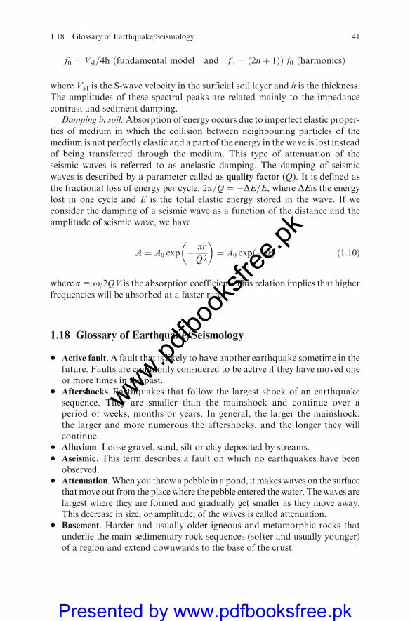
f0 ¼ Vsl=4h ðfundamental model and fn ¼ ð2nþ 1ÞÞ f0 ðharmonicsÞ
where Vs1 is the S-wave velocity in the surficial soil layer and h is the thickness.
The amplitudes of these spectral peaks are related mainly to the impedance
contrast and sediment damping.Damping in soil:Absorption of energy occurs due to imperfect elastic proper-
ties of medium in which the collision between neighbouring particles of the
medium is not perfectly elastic and a part of the energy in the wave is lost instead
of being transferred through the medium. This type of attenuation of the
seismic waves is referred to as anelastic damping. The damping of seismic
waves is described by a parameter called as quality factor (Q). It is defined as
the fractional loss of energy per cycle, 2p=Q ¼ �DE=E, where DEis the energylost in one cycle and E is the total elastic energy stored in the wave. If we
consider the damping of a seismic wave as a function of the distance and the
amplitude of seismic wave, we have
A ¼ A0 exp �prQl
� �¼ A0 expð�arÞ (1:10)
where a=o/2QV is the absorption coefficient. This relation implies that higher
frequencies will be absorbed at a faster rate.
1.18 Glossary of Earthquake/Seismology
� Active fault. A fault that is likely to have another earthquake sometime in thefuture. Faults are commonly considered to be active if they have moved oneor more times in the past.
� Aftershocks. Earthquakes that follow the largest shock of an earthquakesequence. They are smaller than the mainshock and continue over aperiod of weeks, months or years. In general, the larger the mainshock,the larger and more numerous the aftershocks, and the longer they willcontinue.
� Alluvium. Loose gravel, sand, silt or clay deposited by streams.� Aseismic. This term describes a fault on which no earthquakes have been
observed.� Attenuation.When you throw apebble in a pond, itmakeswaves on the surface
thatmove out from the place where the pebble entered the water. The waves arelargest where they are formed and gradually get smaller as they move away.This decrease in size, or amplitude, of the waves is called attenuation.
� Basement. Harder and usually older igneous and metamorphic rocks thatunderlie the main sedimentary rock sequences (softer and usually younger)of a region and extend downwards to the base of the crust.
1.18 Glossary of Earthquake/Seismology 41
www.pdfbo
oksfr
ee.pk
Presented by www.pdfbooksfree.pk

� Bedrock. Relatively hard, solid rock that commonly underlies softer rock,sediment or soil; a subset of the basement.
� Benioff zone. A dipping planar (flat) zone of earthquakes that is produced bythe interaction of a downgoing oceanic crustal plate with a continental plate.These earthquakes can be produced by slip along the subduction thrust faultor by slip on faults within the downgoing plate as a result of bending andextension as the plate is pulled into the mantle. Also known as the Wadati–Benioff zone.
� Body wave. A seismic wave that moves through the interior of the Earth,as opposed to the surface waves that travel near the Earth’s surface. P- andS-waves are body waves.
� Core. The innermost part of the Earth. The outer core extends from 2,500 to3,500miles below the Earth’s surface and is liquidmetal. The inner core is thecentral 500 miles and is solid metal.
� Crust. The outermost major layer of the Earth, ranging from about 10 to65 km in thickness worldwide. The uppermost 15–35 km of crust is brittleenough to produce earthquakes.
� Earthquake. This term is used to describe both sudden slip on a fault and theresulting ground shaking and radiated seismic energy caused by the slip, orby volcanic or magmatic activity, or other sudden stress changes in theEarth.
� Earthquake hazard. Anything associated with an earthquake that may affectthe normal activities of people. This includes surface faulting, ground shak-ing, landslides, liquefaction, tectonic deformation, tsunamis and seiches.
� Earthquake risk. The probable building damage and number of people thatare expected to be hurt or killed if a likely earthquake on a particular faultoccurs. Earthquake risk and earthquake hazard are occasionally usedinterchangeably.
� Epicentre. The point on the Earth’s surface vertically above the point in thecrust where seismic rupture begins.
� Fault. A fracture along which the blocks of crust on either side have movedrelative to one another parallel to the fracture. Strike-slip faults are vertical(or nearly vertical) fractures where the blocks have mostly moved horizon-tally. If the block opposite to an observer looking across the fault moves tothe right, the slip style is termed right-lateral; if the block moves to the left,the motion is termed left-lateral. Dip-slip faults are inclined fractures wherethe blocks have mostly shifted vertically. If the rock mass above an inclinedfault moves down, the fault is termed normal, whereas if the rock above thefault moves up, the fault is termed reverse (or thrust). Oblique-slip faults havesignificant components of both slip styles.
� Foreshocks. Foreshocks are relatively smaller earthquakes that precede thelargest earthquake in a series, which is termed the mainshock. Not allmainshocks have foreshocks.
� Hypocentre. The point within the Earth where an earthquake rupture starts.Also commonly termed the focus.
42 1 Introduction to Earthquake with Explanatory Data
www.pdfbo
oksfr
ee.pk
Presented by www.pdfbooksfree.pk

� Intensity. A number (written as a Roman numeral) describing the severity ofan earthquake in terms of its effects on the Earth’s surface and on humansand their structures. There are many intensity values for an earthquake,depending on where you are, unlike the magnitude, which is one number foreach earthquake.
� Intraplate and crust plate. Intraplate pertains to process within the Earth’scrustal plates. Interplate pertains to process between the plates.
� Isoseismal. A contour or line on amap bounding points of equal intensity fora particular earthquake.
� Left-lateral. If you were to stand on the fault and look along its length, this isa type of strike-slip fault where the left block moves towards you and theright block moves away.
� Lithosphere. The outer solid part of the Earth, including the crust anduppermost mantle. The lithosphere is about 100 km thick, although itsthickness is age dependent (older lithosphere is thicker). The lithospherebelow the crust is brittle enough at some locations to produce earthquakesby faulting, such as within a subducted oceanic plate.
� Love wave. A type of seismic surface wave having a horizontal motion that istransverse (or perpendicular) to the direction the wave is travelling.
� Magnitude. A number that characterizes the relative size of an earthquake.Magnitude is based on measurement of the maximum motion recorded by aseismograph. Several scales have been defined, but the most commonly usedare (1) local magnitude (ML), commonly referred to as ‘‘Richter magnitude’’,(2) surface wave magnitude (MS), (3) body wave magnitude (MB) and (4)moment magnitude (MW).
� Mainshock. The largest earthquake in a sequence, sometimes preceded byone or more foreshocks and almost always followed by many aftershocks.
� Mantle. The part of the Earth’s interior between the metallic outer core andthe crust.
� Moho. The boundary between the crust and the mantle in the Earth. Theboundary is between 25 and 60 km deep beneath the continents and between5 and 10 km deep beneath the ocean floor.
� Oceanic spreading ridge. A fracture zone along the ocean bottom wheremolten mantle material comes to the surface, thus creating new crust. Thisfracture can be seen beneath the ocean as a line of ridges that form as moltenrock reaches the ocean bottom and solidifies.
� Oceanic trench. A linear depression of the sea floor caused by the subductionof one plate under another.
� P-wave. A seismic body wave that shakes the ground back and forth in thesame direction and the opposite direction as the wave is moving.
� Plate tectonics. A theory supported by a wide range of evidence thatconsiders the Earth’s crust and upper mantle to be composed of severallarge, thin, relatively rigid plates that move relative to one another. Slip onfaults that define the plate boundaries commonly results in earthquakes.Several styles of faults bound the plates, including thrust faults along
1.18 Glossary of Earthquake/Seismology 43
www.pdfbo
oksfr
ee.pk
Presented by www.pdfbooksfree.pk

which plate material is subducted or consumed in the mantle, oceanicspreading ridges along which new crystal material is produced and trans-form faults that accommodate horizontal slip (strike-slip) between adjoin-ing plates.
� Rayleigh wave. A seismic surface wave causing the ground to shake in anelliptical motion, with no transverse or perpendicular motion.
� Recurrence interval. The average time span between large earthquakes at aparticular site. Also termed return period.
� Reflection. The energy or wave from an earthquake that has been returned(reflected) from a boundary between two different materials within theEarth, just as a mirror reflects light.
� Refraction. The deflection, or bending, of the ray path of a seismic wavecaused by its passage from one material to another having different elasticproperties. Bending of a tsunami wave front owing to variations in the waterdepth along a coastline.
� Right-lateral. If you were to stand on the fault and look along its length, thisis a type of strike-slip fault where the right block moves towards you and theleft block moves away.
� Ring of fire. The zone of earthquakes surrounding the Pacific Ocean which iscalled the Circum-Pacific belt, about 90% of the world’s earthquakes occurthere. The next most seismic region (5–6% of earthquakes) is the Alpide belt(extends from Mediterranean region, eastwards through Turkey, Iran andnorthern India).
� S-wave. A seismic body wave that shakes the ground back and forth perpen-dicular to the direction the wave is moving, also called a shear wave.
� Sand boil. Sand and water that come out onto the ground surface during anearthquake as a result of liquefaction at shallow depth.
� Seismic gap. A section of a fault that has produced earthquakes in the pastbut is now quiet. For some seismic gaps, no earthquakes have been observedhistorically, but it is believed that the fault segment is capable of producingearthquakes on some other basis, such as plate-motion information or strainmeasurements.
� Seismicity. The geographic and historical distribution of earthquakes.� Seismic moment. A measure of the size of an earthquake based on the area of
fault rupture, the average amount of slip and the force that was required toovercome the friction sticking the rocks together that were offset by faulting.Seismic moment can also be calculated from the amplitude spectra of seismicwaves.
� Seismic zone. An area of seismicity probably sharing a common cause.Example: ‘‘The Himalayan Zone’’.
� Seismogenic. Capable of generating earthquakes.� Seismogram. A recordwritten by a seismograph in response togroundmotions
produced by an earthquake, explosion or other ground motion sources.� Seismology. The study of earthquakes and the structure of the Earth by both
naturally and artificially generated seismic waves.
44 1 Introduction to Earthquake with Explanatory Data
www.pdfbo
oksfr
ee.pk
Presented by www.pdfbooksfree.pk

1.19 Artificial Generation of Earthquake
Back in the period of cold war, the Soviet Union (now Russia), along with the
satellite countries, developed a methodology for the creation of underground
warfare. The basis of this warfare was the artificial generation of earthquakes of
any magnitude, their intention was to destroy ALASKA by reactivating the live
or dead fault lines. Depending on the depth of placing nuclear explosives, the
main concept was to produce various energy waves. The fault lines can easily be
re-activated. This was treated as the cheapest way to destroy any part of a
country with sensative establishment. To a large extent this research was a
success. ALASKAwas onetime a part of Soviet Union and was sold to America.
It was by Soviet Union as a great danger, owing to its close proximity. In case of
the Third World War, they could easily have destroyed ALASKA without the
world knowing that who was responsible.To create successfully on environment for the artificial generation of earth-
quake, the following parameters are essentially to be known as indicated from
the archives:
1. Site survey and geological maps inclusive of the geometry of fault lines.2. Aseismic data and data of aftershock.3. Possibilities of sudden slip on a fault line.4. Tactonic data and soil samples plates.5. Epicentre and Hypocentre data of past earthquakes if any. Site seismology.6. The depth of placement to produce required energy and waves from nuclear
explosives.7. Seismic Zones inclusive of faults and their geometry and positioning.8. The method of production and direction’s of waves.9. Seismograph.
10. The nature and magnitude and producing waves.11. The calculation of wave intensity.12. Control of the waves to the extent demanded.13. Instrumentations and Equipment related to.
1.20 Net Result
This technology has not been effectively tried. However it is a widespread
believe that one portion of Kashmir, known as AZAD KASHMIR, had been
experimented upon successfully. One occupied part of Kashmir was turned out
to be safe while AZAD KASHMIR was totally destroyed.
1.20 Net Result 45
www.pdfbo
oksfr
ee.pk
Presented by www.pdfbooksfree.pk

Bibliography
Abe, K. Tsunami and mechanism of great earthquakes. Phys. Earth Planet Interiors 1973;7:143–153.
Aki, K. Local site effects on strong ground motion. In Earthquake Engineering and SoilDynamics II – Recent Advances in Ground Motion Evaluation (Von Thun, J. L., ed.),Geotechnical Special Publication No. 20, 103–155, American Society of Civil Engineering,New York, 1988.
Aki, K., and Chouet, B. Origin of coda waves: Source, attenuation and scattering effects.J. Geophys. Res. 1975; 80: 3322.
Algermisen, S.T., and Perkins, D.M. A technique for seismic zoning-general considerationand parameter. In Proceedings of the International Conference of Microzonation forSafer-Construction, Research and Application, Vol. II, pp. 865–878, Seattle, Washington,1972.
Ambraseys, N.N. The correlation of intensity with ground motions. In Advances in Engineer-ing Seismology in Europe, Trieste, 1974.
Barazangi, M., and Dorman, J. World seismicity map compiled from ESSA, coat andgeodetic survey, epicenter data, 1961–1967. Bull. Seismol. Soc. Am. 1969; 59:369–380.
Bard, P.Y., and Bouchon,M. The seismic response of sediment-filled valleys – Part 1: The caseof incident SH waves. Bull. Seismol. Soc. Am. 1980a; 70: 1263–1286.
Bard, P.Y., and Bouchon,M. The seismic response of sediment-filled valleys – Part 2: The caseof incident P and SV waves. Bull. Seismol. Soc. Am. 70: 1921–1941, 1980b.
Bard, P.Y., and Bouchon, M. The two-dimensional resonance of sediment-filled valleys. Bull.Seismol. Soc. Am. 1985; 75: 519–541.
Basu, S. Statistical analysis of seismic data and seismic risk analysis of Indian Peninsula.Ph.D. thesis, Department of Civil Engineering, IIT Kanpur, India, 1977.
Bath, M. Earthquake energy and magnitude. Phys. Chem. Earth. Ahren, L.H. Press, 1966;115–165.
Bolt, B.A., and Abrahamson, N.A. New attenuation relations for peak and expected accel-erations of ground motion. Bull. Seismol. Soc. Am. 1982; 72, 2307–2321.
Boore, D.M., Joyner, W.B., and Fumal, T.E. Equations for estimating horizontal responsespectra and peak acceleration for western north American earthquakes: A summary ofrecent works. Seismol. Res. Lett. 1997; 68(1), 128–140.
Bullen, E., and Bolt, B.A. An Introduction to the Theory of Seismology, Cambridge UniversityPress, Cambridge, 1985.
Burridge, R., and Knopoff, L. Body force equivalents for seismic dislocation. Bull. Seismol.Soc. Am. 54: 1875–1888, 1964.
Campbell, K.W. Empirical near-source attenuation relationships for horizontal and verticalcomponents of peak ground acceleration, Peak Ground Velocity, and Pseudo-absoluteAcceleration Response Spectra. Seismol. Res. Lett. 1997; 68(1), 154–179.
Celebi, M. Topographical and geological amplifications determined from strong-motion andaftershock records of the 3March 1985 Chile earthquake.Bull. Seismol. Soc. Am. 1987; 77:1147–1167.
Conrad, V., Laufzeitkurven Des Tauernbebens, vom 28: 59: 1–23,Mitt. Erdb. –Komm.Wien,1925.
Cornell, C.A. Engineering seismic risk analysis. Bull. Seismol. Soc. Am. 1968; 58, 1583–1606.DeMets, C. et al. Curr. Plate Motions 1990; 101, 425–478.Esteva, L. Bases Para la Formulacion de Decisiones de Diseno Sismico. Technical Report,
INstitute de Ingenieria, UNAM, Mexico, 1968.Esteva, L., and Villaverde, R. Seismic risk design spectra and structural reliability.
In Proceedings of the Fifth World Conference on Earthquake Engineering, Rome,pp. 2586–2596, 1974.
46 1 Introduction to Earthquake with Explanatory Data
www.pdfbo
oksfr
ee.pk
Presented by www.pdfbooksfree.pk

Faccioli, E., Seismic Amplification in the presence of geological and topographic irre-gularities. Proceedings of the 2nd International Conference on Recent Advances inGeotechnical Earthquake Engineering and Soil Dynamics, St. Louis, Missouri, 1991;2: 1779–1797.
Geli, L., Bard, P.Y., and Jullien, B. The effect of topography on earthquake groundmotion: Areview and new results. Bull. Seismol. Soc. Am. 1988; 78: 42–63.
Gutenberg, B. The Energy of Earthquakes 1945; 112: 1–14.Gutenberg, B. Magnitude determination for deep focus earthquakes. Bull. Seismol. Soc. Am.
1956; 35: 117–130.Gutenberg, B., and Richter, C.F., Seismicity of Earth and Related Phenomenon, Princeton
University Press, Princeton, NJ, 1945.Hanks, T.C., and Kanamori, H. A moment magnitude scale. J. Geophys. Res. 1979; 84(B5),
2348–2350.Hatayama, K., Matsunami, K. Iwata, T., and Irikura, K. Basin-induced love wave in the
eastern part of the Osaka basin. J. Phys. Earth 1995; 43, 131–155.Housner, G.W. Calculating the response of an oscillator to arbitrary ground motion. Bull.
Seismol. Soc. Am. 31: 143–149, 1941.Housner, G.W.Measures of severity of earthquake ground shaking. In Proceedings of the US
National Conference on Earthquake Engineering, Earthquake Engineering Institute, AnnArbor, Michigan, pp. 25–33, 1975.
Hutton, L.K., and Boore, D.M. The M scale in Southern California. Bull. Seismol. Soc. Am.77: 6: 2074–2094, 1987.
IS:1893. Indian Standard Criteria for Earthquake Resistant Design of Structures, Part 1,Bureau of Indian Standards, New Delhi, 2002.
Jibson, R. Summary on research on the effects of topographic amplification of earthquakeshaking on slope stability. Open-File-Report-87-268, USGS, California, 1987.
Joyner,W.B., and Boore, D.M. Peak horizontal acceleration and velocity from strong-motionrecords including records from the 1979 Imperial Valley, California Earthquake. Bull.Seismol. Soc. Am. 71: 2011–2038, 1981.
Kanamori, H. Mechanisms of tsunami earthquake. Phys. Planet Interiors 1972; 6, 246–259.Kanamori, H. The energy release in great earthquakes. Tectonophysics 1977; 93, 185–199.Kawase, H. The cause of damage belt in Kobe: ‘The basin-edge effect’, constructive inter-
ference of the direct S-waves with the basin induced diffracted/Rayleigh waves. Seismol.Res. Lett. 1996; 67, 25–34.
Kawase, H., and Aki, K. Topography effect at the critical SV wave incidence: Possibleexplanation of damage pattern by the Whitter narrow. Earthquake of 1 October 1987.Bull. Seismol. Soc. Am. 1990; 80: 1–22, California.
Kennet, B.L.N., and Engdahl, E.R. Trabel ties for global earthquake location and phaseidentification. Int. J. Geophys. 1991; 105, 429–465.
Khan, P.K. Recent seismicity trend in India and adjoining regions. ISET,New Lett., October2003–July 2004, 10–14, 2004.
Kim, W.Y. The M scale in Eastern North America. Bull. Seismol. Soc. Am. 1998; 88,935–951.
Langston, C.A. Brazier, R., Nyblade, A.A., and Owens, T.J. Local magnitude scale andseismicity rate for Tanzania, East Africa. Bull. Seismol. Soc. Am. 1998; 88, 712–721.
Levret, A., Loup, C., and Goula, X. The Provence Earthquake of June 11, 1909 (France):New assessment of near field effects. Proceedings of the 8th European Conference ofEarthquake Engineering, Lisbon, 2, p. 4.2.79, 1986.
Love, A.E.H. Some Problems of Aerodynamics, Cambridge University Press, Cambridge,1911.
Lowrie, W., Fundamentals of Geophysics, Cambridge University Press, Cambridge, 1997.MacMurdo, J. Papers relating to the earthquake which occurred in India in 1819.Philos.Mag.
1824; 63, 105–177.
Bibliography 47
www.pdfbo
oksfr
ee.pk
Presented by www.pdfbooksfree.pk

Maruyama, T. On the force equivalents of dynamic elastic dislocations with reference to theearthquake mechanism. Bulletin of Earthquake Research Institute, Tokyo University 1963;41, 467–486.
McGuire, R.K. Seismic design spectra and mapping procedures using hazard analysis baseddirectly on oscillator response. Earthquake Eng. Struct. Dyn. 1977; 5, 211–234.
Moczo, P., and Bard, P.Y. Wave diffraction, amplification and differential motion nearstrong lateral discontinuities. Bull. Seismol. Soc. Am. 83: 85–106, 1993.
Mohorovicic, A. Das Beben Vom 8 x 1909. Jb. Met. Obs. Zagreb 1909; 9, 1–63.Mohraz, B. A study of earthquake response spectra for different geologic condition. Bull.
Seismol. Soc. Am. 66: 915–932, 1976.Murphy, J.R., and O’Brien, L.J. The correlation of peak ground acceleration amplitude
with seismic intensity and other physical parameters. Bull. Seismol. Soc. Am. 1977; 67,877–915.
Mussett, A.E., and Khan, M.A., Looking into the Earth: An Introduction to GeologicalGeophysics. Cambridge University Press, Cambridge, 2000.
Narayan, J.P, Sharma, M.L., and Ashwani K. A Seismological Report on the January 26,2001 Bhuj, India Earthquake. Seismol. Res. Lett. 2002; 73, 343–355.
Narayan, J.P. 2.5D Simulation of basin-edge effects on the ground motion characteristics.Proc. Indian Acad. Sci. (Science of the Earth Planet), 2003a; 112: 463–469.
Narayan, J.P. 3D Simulation of basin-edge effects on the ground motion characteristics.13WCEE, August 1–6, Paper No. 3333, Vancouver, Canada, 2004.
Narayan, J.P. Simulation of ridge weathering effects on the ground motion characteristics.J. Earthquake Eng. 2003b; 7: 447–461.
Narayan, J.P. Study of basin-edge effects on the ground motion characteristics using 2.5-Dmodelling. Pure Appl. Geophys. 2005; 162, 273–289.
Narayan, J.P., and Prasad Rao, P.V. Two and half dimensional simulation of ridge effects onthe ground motion characteristics. Pure Appl. Geophys. 2003; 160, 1557–1571.
Narayan, J.P., and Rai, D.C. An observational study of local site effects in the Chamoli earth-quake. Proceedings of Workshop on Recent Earthquakes of Chamoli and Bhuj, 273–279, 2001.
Narayan,M.P. Site specific strong groundmotion prediction using 2.5-Dmodelling.Geophys.J. Int. 2001; 146, 269–281.
NEHRP. Recommended Provisions for Seismic Regulation for New Buildings and OtherStructures. Technical Report, Building Safety Council for Federal Emergency Manage-ment, Washington D.C., 1997.
Newmark, N.M. and Rosenblueth, E., Fundamentals of Earthquake Engineering. PrenticeHall, Inc., Englewood Cliffs, NJ, 1971.
Newmark, N.M., and Hall, W.J. Earthquake spectra and design. Technical Report, Earth-quake Engineering Research Institute, Berkeley, California, 1982.
Newmark, N.M., Blume, J.A., and Kapur, K.K. Seismic design spectra for nuclear powerplants. J. Power Division, ASCE 1973; 99(02), 873–889.
Oldham, R.D. A catalogue of Indian earthquakes from the earliest times to the end of A.D.1869. Memoir X, Geological Survey of India, 1883.
Oldham, R.D. The constitution of the interior of the earth, as revealed by earthquakes.Quar.J. Geo. Soc. London 1906; 62, 456–75.
Pederson, H., Hatzfield, D., Campillo, M., and Bard, P.Y. Ground motion amplitude acrossridges. Bull. Seismol. Soc. Am. 84: 1786–1800, 1994.
Pitarka, A. Irikura, K., Iwata, T., and Sekiguchi, H. Three-dimensional Simulation of thenear fault ground motion for 1995. Hyogo-ken Nanbu (Kobe), Japan earthquake, Bull.Seismol. Soc. Am. 88: 428–440, 1998.
Plesinger, A., Zmeskal, M., and Zednik, J. Automated Pre-processing of Digital Seismograms:Principles and Software. Version 2.2, E. Bergman (Ed.), Prague and Golden, 1996.
Rayleigh, L. On-wave propagated along the plane surface of an elastic solid. Proc. LondonMath. Soc. 1885; 17, 4–11.
48 1 Introduction to Earthquake with Explanatory Data
www.pdfbo
oksfr
ee.pk
Presented by www.pdfbooksfree.pk

Reid, H.F. The elastic rebound theory of earthquakes. Bull. Dept. Geol 6: 413–444, Universityof Berkeley, 1911.
Reid, H.F., The California Earthquake of April 18, 1906, Publication 87, 21 Carnegie Instituteof Washington, D.C., 1910.
Richter, C.F. An instrumental earthquake magnitude scale. Bull. Seismol. Soc. Am. 25: 1–32,1935.
Richter, C.F., Elementary Seismology. W.H. Freeman and Co., San Francisco, CA, 1958.Sanchez-Sesma, F.J. Elementary solutions for the response of a wedge-shaped medium to
incident SH and SV waves. Bull. Seismol. Soc. Am. 80: 737–742, 1990.Satake, K., Tsunamis, International Handbook of Earthquake and Engineering Seismology-
Part B, Lee et al. (Eds.), 437–451, 2002.Seed, H.B., and Idriss, I.M. Ground motions and soil liquefaction during earthquakes.
Technical Report, Earthquake Engineering Research Institute, Berkeley, California, 1982.Seed, H.B., Ugas, C., and Lysmer, J. Site dependent spectra for earthquake-resistant design.
Bull. Seismol. Soc. Am. 66: 221–243, 1976.Siro, L. Southern Italy November 23, 1980 Earthquake. Proceedings of the 7th European
Conference on Earthquake Engineering, Athens, Greece, 1982.Slemmons, D.B. Determination of design earthquake magnitudes for Microzonation. in
Proceedings of 3rd International EarthquakeMicrozonation Conference, pp. 119–130, 1982.Tocher, D. Earthquake energy and ground breakage. Bull. Seismol. Soc. Am. 1958; 48(2):
147–153.Trifunac, M.D., and Brady, A.G. A study of the duration of strong earthquake ground
motion. Bull. Seismol. Soc. Am. 65: 581–626, 1975.Trifunac, M.D., and Brady, A.G. On the correlation of seismic intensity with peaks of
recorded strong motion. Bull. Seismol. Soc. Am. 65: 139–162, 1975.Wells, D.L., and Coppersmith, K.J. New empirical relationships among magnitude, rupture
length, rupture width, rupture area and surface displacement. Bull. Seismol. Soc. Am.1994; 84(4): 974–1002.
Wood, H.O. Distribution of apparent intensity in San Francisco, in the California Earth-quake of April 18, 1906. Report of the State Earthquake Investigation Commission, 1:220–245, Carnegie Institute of Washington, Washington, D.C., 1908.
Bibliography 49
www.pdfbo
oksfr
ee.pk
Presented by www.pdfbooksfree.pk

www.pdfbo
oksfr
ee.pk
Presented by www.pdfbooksfree.pk
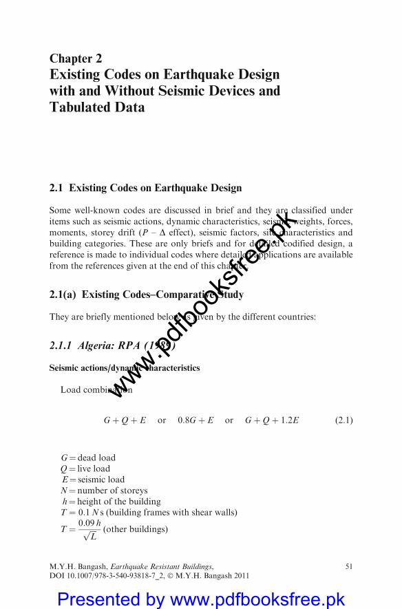
Chapter 2
Existing Codes on Earthquake Design
with and Without Seismic Devices and
Tabulated Data
2.1 Existing Codes on Earthquake Design
Some well-known codes are discussed in brief and they are classified under
items such as seismic actions, dynamic characteristics, seismic weights, forces,moments, storey drift (P – D effect), seismic factors, site characteristics andbuilding categories. These are only briefs and for detailed codified design, areference is made to individual codes where detailed applications are available
from the references given at the end of this chapter.
2.1(a) Existing Codes–Comparative Study
They are briefly mentioned below as given by the different countries:
2.1.1 Algeria: RPA (1989)
Seismic actions/dynamic characteristics
Load combination
GþQþ E or 0:8G þ E or GþQþ 1:2E (2:1)
G¼ dead loadQ¼ live loadE¼ seismic loadN¼ number of storeysh¼ height of the buildingT ¼ 0:1N s (building frames with shear walls)
T ¼ 0:09 hffiffiffiffiLp (other buildings)
M.Y.H. Bangash, Earthquake Resistant Buildings,DOI 10.1007/978-3-540-93818-7_2, � M.Y.H. Bangash 2011
51
www.pdfbo
oksfr
ee.pk
Presented by www.pdfbooksfree.pk
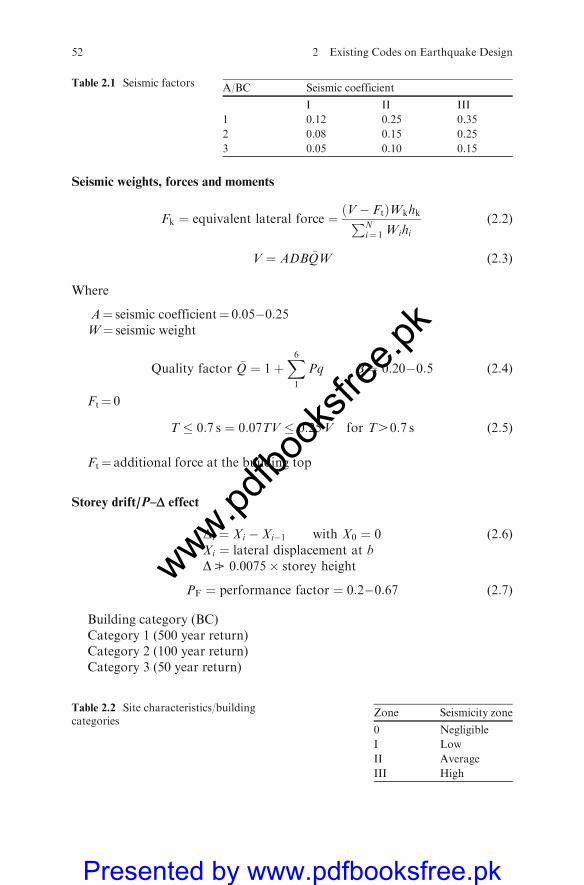
Seismic weights, forces and moments
Fk ¼ equivalent lateral force ¼ V� Ftð ÞWkhkPNi¼ 1 Wihi
(2:2)
V ¼ ADB �QW (2:3)
Where
A¼ seismic coefficient¼ 0.05�0.25W¼ seismic weight
Quality factor �Q ¼ 1þX61
Pq B ¼ 0:20�0:5 (2:4)
Ft¼ 0
T � 0:7 s ¼ 0:07TV � 0:25V for T40:7 s (2:5)
Ft¼ additional force at the building top
Storey drift/P–D effect
Di ¼ Xi � Xi�1 with X0 ¼ 0 (2:6)Xi ¼ lateral displacement at bDB 0:0075� storey height
PF ¼ performance factor ¼ 0:2�0:67 (2:7)
Building category (BC)Category 1 (500 year return)Category 2 (100 year return)Category 3 (50 year return)
Table 2.2 Site characteristics/buildingcategories
Zone Seismicity zone
0 Negligible
I Low
II Average
III High
Table 2.1 Seismic factors A/BC Seismic coefficient
I II III
1 0.12 0.25 0.35
2 0.08 0.15 0.25
3 0.05 0.10 0.15
52 2 Existing Codes on Earthquake Design
www.pdfbo
oksfr
ee.pk
Presented by www.pdfbooksfree.pk
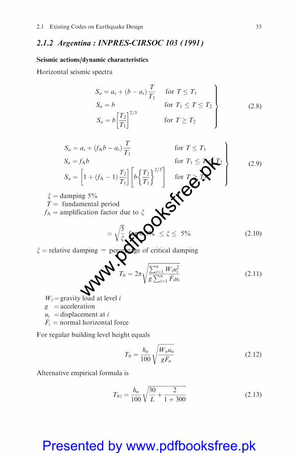
2.1.2 Argentina : INPRES-CIRSOC 103 (1991)
Seismic actions/dynamic characteristics
Horizontal seismic spectra
Sa ¼ as þ ðb� asÞT
T1for T � T1
Sa ¼ b for T1 � T � T2
Sa ¼ bT2
T1
� �2=3for T � T2
9>>>>>=>>>>>;
(2:8)
Sa ¼ as þ ðfAb� asÞT
T1for T � T1
Sa ¼ fAb for T1 � T � T2
Sa ¼ 1þ ðfA � 1ÞT2
T1
� �b
T2
T1
� �2=3" #
for T � T2
9>>>>>=>>>>>;
(2:9)
x ¼ damping 5%T ¼ fundamental periodfA ¼ amplification factor due to x
¼ffiffiffi5
x
rfor 0:5% � x � 5% (2:10)
x ¼ relative damping = percentage of critical damping
T0 ¼ 2p
ffiffiffiffiffiffiffiffiffiffiffiffiffiffiffiffiffiffiffiffiffiffiffiPni¼1Wiu
2i
gPn
i¼1�Fiui
s(2:11)
Wi¼ gravity load at level ig ¼ accelerationui ¼ displacement at i�Fi ¼ normal horizontal force
For regular building level height equals
T0 ¼hn100
ffiffiffiffiffiffiffiffiffiffiffiWnun
g �Fn
s(2:12)
Alternative empirical formula is
T0 l ¼hn100
ffiffiffiffiffiffiffiffiffiffiffiffiffiffiffiffiffiffiffiffiffiffiffiffiffiffiffi30
Lþ 2
1þ 300
r(2:13)
2.1 Existing Codes on Earthquake Design 53
www.pdfbo
oksfr
ee.pk
Presented by www.pdfbooksfree.pk
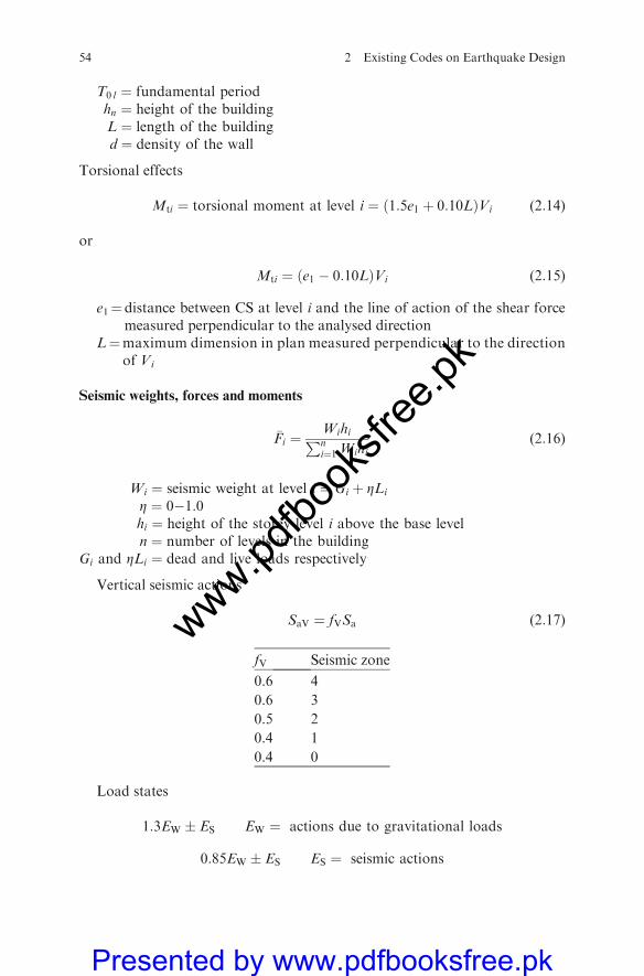
T0 l ¼ fundamental periodhn ¼ height of the buildingL ¼ length of the buildingd ¼ density of the wall
Torsional effects
Mti ¼ torsional moment at level i ¼ ð1:5e1 þ 0:10LÞVi (2:14)
or
Mti ¼ ðe1 � 0:10LÞVi (2:15)
e1¼ distance between CS at level i and the line of action of the shear forcemeasured perpendicular to the analysed direction
L¼maximum dimension in plan measured perpendicular to the directionof Vi
Seismic weights, forces and moments
�Fi ¼WihiPni¼1Wihi
(2:16)
Wi ¼ seismic weight at level i ¼ Gi þ ZLi
Z ¼ 0�1:0hi ¼ height of the storey level i above the base leveln ¼ number of levels in the building
Gi and ZLi ¼ dead and live loads respectively
Vertical seismic actions
SaV ¼ fVSa (2:17)
fV Seismic zone
0.6 4
0.6 3
0.5 2
0.4 1
0.4 0
Load states
1:3EW � ES EW ¼ actions due to gravitational loads
0:85EW � ES ES ¼ seismic actions
54 2 Existing Codes on Earthquake Design
www.pdfbo
oksfr
ee.pk
Presented by www.pdfbooksfree.pk
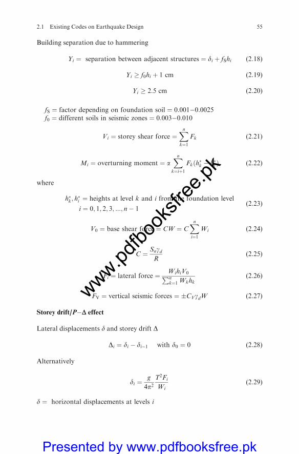
Building separation due to hammering
Yi ¼ separation between adjacent structures ¼ di þ fShi (2:18)
Yi � f0hi þ 1 cm (2:19)
Yi � 2:5 cm (2:20)
fS ¼ factor depending on foundation soil ¼ 0:001�0:0025f0 ¼ different soils in seismic zones ¼ 0:003�0:010
Vi ¼ storey shear force ¼Xnk¼1
Fk (2:21)
Mi ¼ overturning moment ¼ aXnk¼iþ1
Fkðh�k � h�i Þ (2:22)
where
h�k; h�i ¼ heights at level k and i from the foundation level
i ¼ 0; 1; 2; 3; :::; n� 1(2:23)
V0 ¼ base shear force ¼ CW ¼ CXni¼1
Wi (2:24)
C ¼ SagdR
(2:25)
Fi ¼ lateral force ¼ WihiV0Pnk¼1 Wkhk
(2:26)
FV ¼ vertical seismic forces ¼ �CVgdW (2:27)
Storey drift/P�D effect
Lateral displacements d and storey drift D
Di ¼ di � di�1 with d0 ¼ 0 (2:28)
Alternatively
di ¼g
4p2T2Fi
Wi(2:29)
d ¼ horizontal displacements at levels i
2.1 Existing Codes on Earthquake Design 55
www.pdfbo
oksfr
ee.pk
Presented by www.pdfbooksfree.pk
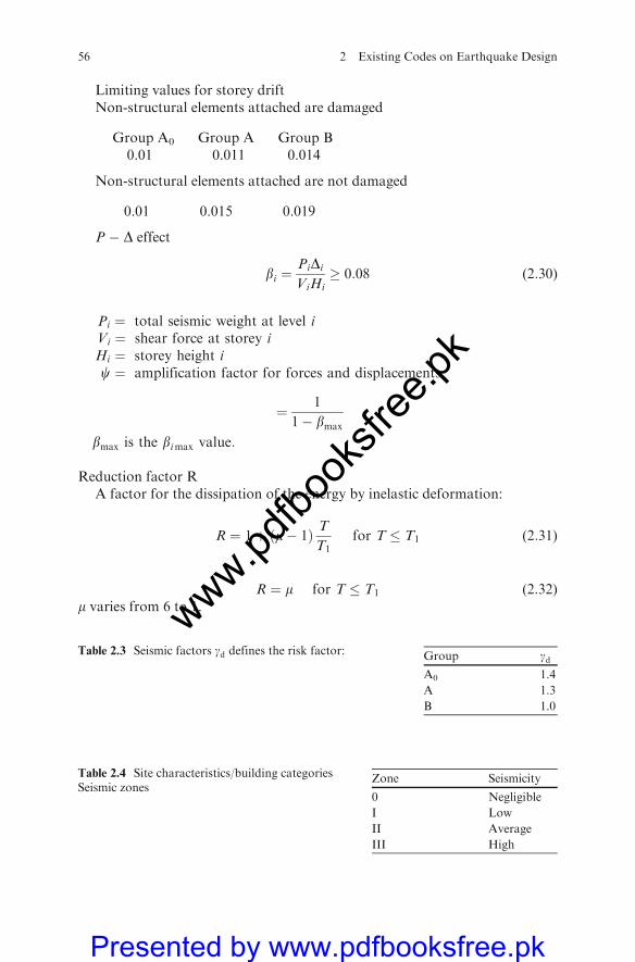
Limiting values for storey driftNon-structural elements attached are damaged
Group A0 Group A Group B0.01 0.011 0.014
Non-structural elements attached are not damaged
0.01 0.015 0.019
P � D effect
bi ¼PiDi
ViHi� 0:08 (2:30)
Pi ¼ total seismic weight at level iVi ¼ shear force at storey iHi ¼ storey height ic ¼ amplification factor for forces and displacements
¼ 1
1� bmax
bmax is the bimax value:
Reduction factor RA factor for the dissipation of the energy by inelastic deformation:
R ¼ 1þ ðm� 1Þ TT1
for T � T1 (2:31)
R ¼ m for T � T1 (2:32)m varies from 6 to 1.
Table 2.4 Site characteristics/building categoriesSeismic zones
Zone Seismicity
0 Negligible
I Low
II Average
III High
Table 2.3 Seismic factors gd defines the risk factor: Group gdA0 1.4
A 1.3
B 1.0
56 2 Existing Codes on Earthquake Design
www.pdfbo
oksfr
ee.pk
Presented by www.pdfbooksfree.pk
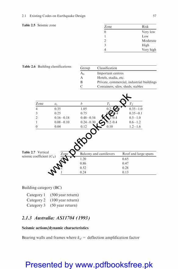
Building category (BC)
Category 1 (500 year return)
Category 2 (100 year return)
Category 3 (50 year return)
2.1.3 Australia: AS11704 (1993)
Seismic actions/dynamic characteristics
Bearing walls and frames where kd = deflection amplification factor
Table 2.5 Seismic zone Zone Risk
0 Very low
1 Low
2 Moderate
3 High
4 Very high
Table 2.7 Verticalseismic coefficient (CV)
Zone Balcony and cantilevers Roof and large spans
4 1.20 0.65
3 0.86 0.47
2 0.52 0.28
1 0.24 0.13
Zone as b T1 T2
4 0.35 1.05 0.2�0.4 0.35�1.03 0.25 0.75 0.2�0.4 0.35�0.12 0.16�0.18 0.48�0.54 0.2–0.4 0.5�1.01 0.08�0.10 0.24�0.30 0.2–0.4 0.6�1.20 0.04 0.12 0.10 1.2�1.6
Table 2.6 Building classifications Group Classification
A0 Important centres
A Hotels, stadia, etc.
B Private, commercial, industrial buildings
C Containers, silos, sheds, stables
2.1 Existing Codes on Earthquake Design 57
www.pdfbo
oksfr
ee.pk
Presented by www.pdfbooksfree.pk
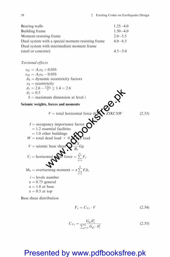
Bearing walls 1.25�4.0Building frame 1.50�4.0Moment-resisting frame 2.0�5.5Dual system with a special moment-resisting frame 4.0�6.5Dual system with intermediate moment frame
(steel or concrete) 4.5�5.0
Torsional effects
ed1 ¼ A1eS þ 0:05bed2 ¼ A2eS � 0:05bAS ¼ dynamic eccentricity factorseS ¼ eccentricityA1 ¼ 2:6� 3:6eS
b � 1:4 ¼ 2:6A2 ¼ 0:5b ¼ maximum dimension at level i
Seismic weights, forces and moments
V ¼ total horizontal force (kN) ¼ ZIKCSW (2:33)
I ¼ occupancy importance factor¼ 1.2 essential facilities¼ 1.0 other buildings
W ¼ total dead load + 0.25 live load
V ¼ seismic base shear ¼ ICS
RfGg
Vi ¼ horizontal shear force ¼Pnx¼i
Fx
M0 ¼ overturning moment ¼ aPni¼1
Fihi
i ¼ levels numbera ¼ 0:75 generala ¼ 1:0 at basea ¼ 0:5 at top
Base shear distribution
Fx ¼ CVx � V (2:34)
CVx ¼Ggsh
kxPn
i¼1Ggi � hki(2:35)
58 2 Existing Codes on Earthquake Design
www.pdfbo
oksfr
ee.pk
Presented by www.pdfbooksfree.pk

x ¼ i levelsk ¼ 1 T � 0:5 s
Gg ¼ gravity load ¼ Gþ cQG ¼ dead load (kN)Q ¼ live load (kN)
Storey drift/P�D effect
dx ¼ interstorey drift ¼ kddxedxe ¼ lateral displacement at levels i
(2:36)
¼ aiT
2p
� �2
¼ gFi
Ggi
T
2p
� �2
(2:37)
P�D effectTo allow for P�D effect, the storey drift is increased by
0:9
ð1�mÞ � 1:0 (2:38)
When m50:1 there is no effect
m ¼ stability coefficient ¼ PxDx
Vxhsxkd(2:39)
Px ¼ total vertical design load
Seismic factors
C ¼ seismic response factor ¼ 1
15ffiffiffiffiTp � 0:12 (2:40)
a ¼ acceleration coefficient ¼ 0:05�0:11
C ¼ 1:25a
T2=3(2:41)
T ¼ h046
(main direction) (2:42)
T ¼ h0
58(orthogonal direction) (2:43)
c ¼ 0:4�0:6Rf ¼ response modification factor ¼ 1:5�8:0
2.1 Existing Codes on Earthquake Design 59
www.pdfbo
oksfr
ee.pk
Presented by www.pdfbooksfree.pk

k ¼ horizontal force factor¼ 0:75 ðductileÞ¼ 3:2 ðbrittleÞ
Z ¼ zone factor¼ 0 for zone A ductile¼ 0:09 for zone A non-ductile¼ 0:18 for zone 1¼ 0:36 for zone 2
Site characteristics/building categories
S ¼ soil structure resonance factor ¼ 1:5 if not calculated
Building classification
Type I Domestic and not more than two storeys
Type II Buildings with high occupancy (schools, theatres, etc.)
Type III Buildings for essential functions (power stations, tall structures,hospitals, etc.)
C¼ static analysisD¼ static and dynamic analysisE¼ static and dynamic analysisS¼ site factor varies from 0.67 to 2.0
2.1.4 China: TJ 11-78 and GBJ 11-89
Seismic actions/dynamic characteristics
S ¼ total effect of horizontal seismic action
¼
ffiffiffiffiffiffiffiffiffiffiffiffiffiXNj¼1
S2j
vuut (2:44)
T1 ¼ fundamental periodSj ¼ modal effect caused by seismic forces of the jth modeN ¼ number of modes
Table 2.8 Seismic design categories
aS III II I Domestic
aS � 0:20 E D C H3
0:10 � aS � 0:20 D C B H2
aS50:10 C B A H1
60 2 Existing Codes on Earthquake Design
www.pdfbo
oksfr
ee.pk
Presented by www.pdfbooksfree.pk
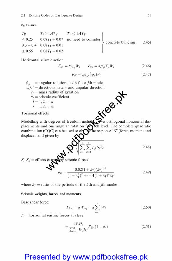
dn values
Tg T141:47 g T1 � 1:4Tg
� 0:25 0:08T1 þ 0:07 no need to consider
0:3� 0:4 0:08T1 þ 0:01
� 0:55 0:08T1 � 0:02
9>>>=>>>;
concrete building (2:45)
Horizontal seismic action
Fxji ¼ ajgtjWi Fyji ¼ ajgtjYjiWi (2:46)
Ftji ¼ ajgtjr2i fjiWi (2:47)
fji ¼ angular rotation at ith floor jth modex; j; t ¼ directions in x; y and angular direction
ri ¼ mass radius of gyrationaj ¼ seismic coefficienti ¼ 1; 2; :::; nj ¼ 1; 2; :::;m
Torsional effects
Modelling with degrees of freedom including two orthogonal horizontal dis-placements and one angular rotation for each level. The complete quadraticcombination (CQC) can be used to obtain the response ‘‘S’’ (force, moment anddisplacement) given by
S ¼
ffiffiffiffiffiffiffiffiffiffiffiffiffiffiffiffiffiffiffiffiffiffiffiffiffiffiffiffiffiffiXnj¼1
Xnk¼1
rjkSjSk
vuut (2:48)
Sj;Sk ¼ effects caused by seismic forces
rjk ¼0:02ð1þ lTÞðlTÞ1:5
ð1� l2TÞ2 þ 0:01ð1þ lTÞ2lT
(2:49)
where lT ¼ ratio of the periods of the kth and jth modes.
Seismic weights, forces and moments
Base shear force:
FEK ¼ aWeq ¼ aXni¼1
Wi (2:50)
Fi¼ horizontal seismic forces at i level
¼ WiHiPnj¼1 WjHj
FEKð1� dnÞ (2:51)
2.1 Existing Codes on Earthquake Design 61
www.pdfbo
oksfr
ee.pk
Presented by www.pdfbooksfree.pk
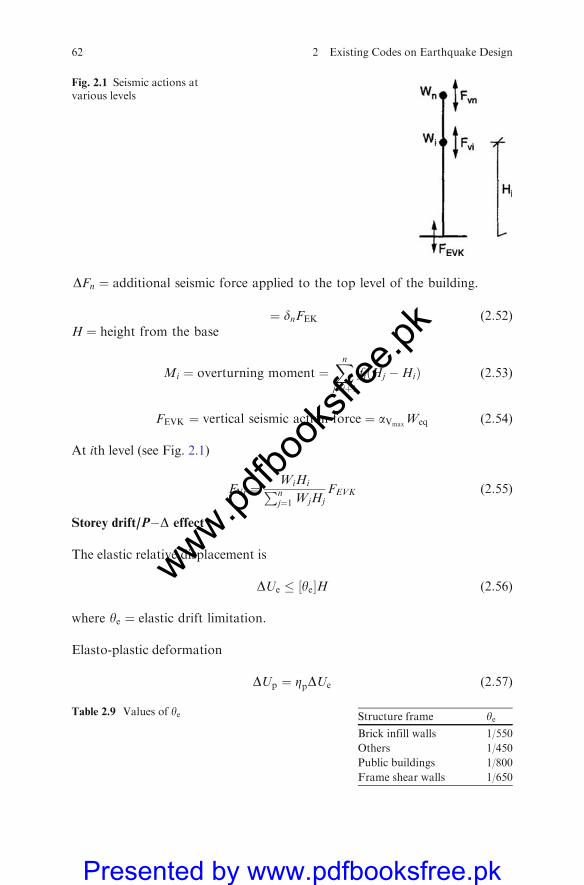
DFn ¼ additional seismic force applied to the top level of the building.
¼ dnFEK (2:52)H ¼ height from the base
Mi ¼ overturning moment ¼Xnj¼iþ1
fjðHj �HiÞ (2:53)
FEVK ¼ vertical seismic action force ¼ aVmaxWeq (2:54)
At ith level (see Fig. 2.1)
FVi ¼WiHiPnj¼1 WjHj
FEVK (2:55)
Storey drift/P�D effect
The elastic relative displacement is
DUe � ye½ H (2:56)
where ye ¼ elastic drift limitation.
Elasto-plastic deformation
DUp ¼ ZpDUe (2:57)
Table 2.9 Values of ye Structure frame yeBrick infill walls 1/550
Others 1/450
Public buildings 1/800
Frame shear walls 1/650
Fig. 2.1 Seismic actions atvarious levels
62 2 Existing Codes on Earthquake Design
www.pdfbo
oksfr
ee.pk
Presented by www.pdfbooksfree.pk

or
DUp ¼ mDUy ¼ZpDUy
xy(2:58)
DUy ¼ storey yield displacementDUe ¼ elastically calculated storey displacementZp ¼ amplification coefficient
Up � yp
H (2:59)
Seismic factors
a ¼ seismic coefficient
a ¼ amaxð5:5T1 þ 0:45Þ for T1 � 0:1s (2:60)
a ¼ amax for 0:15T1 � 0:1Tg
a ¼ Tg
T1
� �0:9
amax for Tg5T153s (2:61)
dn ¼ additional seismic action coefficientgtj ¼ the mode participation factor of the jth moderjk ¼ coupling coefficient for jth and kth modesm ¼ storey ductility coefficient
xy ¼ storey yield strength coefficient ¼ Fy
Qe(2:62)
Table 2.11 amax values for variousintensities
Intensity amax
VI VII VIII IX
0.04 0.08 0.16 0.32
Table 2.10 The value of yp yp Structure
1/30 Single-storey RC frame
1/50 Frame with infill
1/70 Frame in the first storey of a brick building
2.1 Existing Codes on Earthquake Design 63
www.pdfbo
oksfr
ee.pk
Presented by www.pdfbooksfree.pk
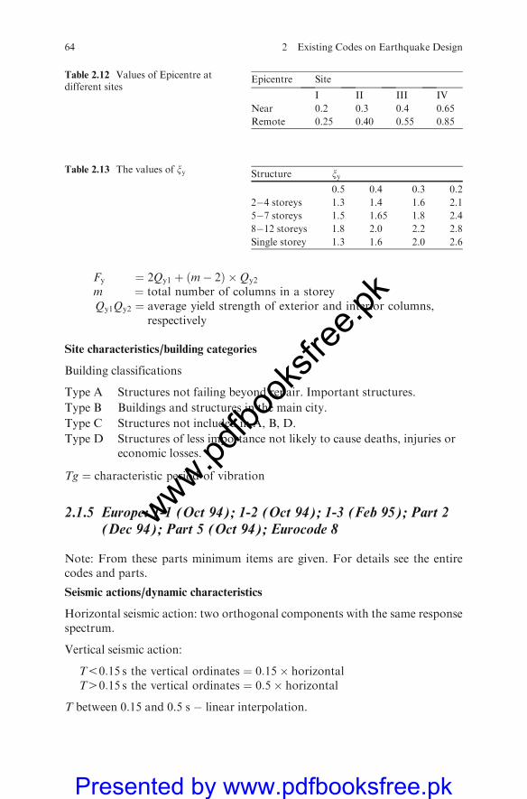
Fy ¼ 2Qy1 þ ðm� 2Þ �Qy2
m ¼ total number of columns in a storeyQy1Qy2 ¼ average yield strength of exterior and interior columns,
respectively
Site characteristics/building categories
Building classifications
Type A Structures not failing beyond repair. Important structures.
Type B Buildings and structures in the main city.
Type C Structures not included in A, B, D.
Type D Structures of less importance not likely to cause deaths, injuries oreconomic losses.
Tg ¼ characteristic period of vibration
2.1.5 Europe: 1-1 (Oct 94); 1-2 (Oct 94); 1-3 (Feb 95); Part 2(Dec 94); Part 5 (Oct 94); Eurocode 8
Note: From these parts minimum items are given. For details see the entirecodes and parts.
Seismic actions/dynamic characteristics
Horizontal seismic action: two orthogonal components with the same responsespectrum.
Vertical seismic action:
T50:15 s the vertical ordinates ¼ 0:15� horizontalT40:15 s the vertical ordinates ¼ 0:5� horizontal
T between 0.15 and 0.5 s � linear interpolation.
Table 2.13 The values of xy Structure xy0.5 0.4 0.3 0.2
2�4 storeys 1.3 1.4 1.6 2.1
5�7 storeys 1.5 1.65 1.8 2.4
8�12 storeys 1.8 2.0 2.2 2.8
Single storey 1.3 1.6 2.0 2.6
Table 2.12 Values of Epicentre atdifferent sites
Epicentre Site
I II III IV
Near 0.2 0.3 0.4 0.65
Remote 0.25 0.40 0.55 0.85
64 2 Existing Codes on Earthquake Design
www.pdfbo
oksfr
ee.pk
Presented by www.pdfbooksfree.pk
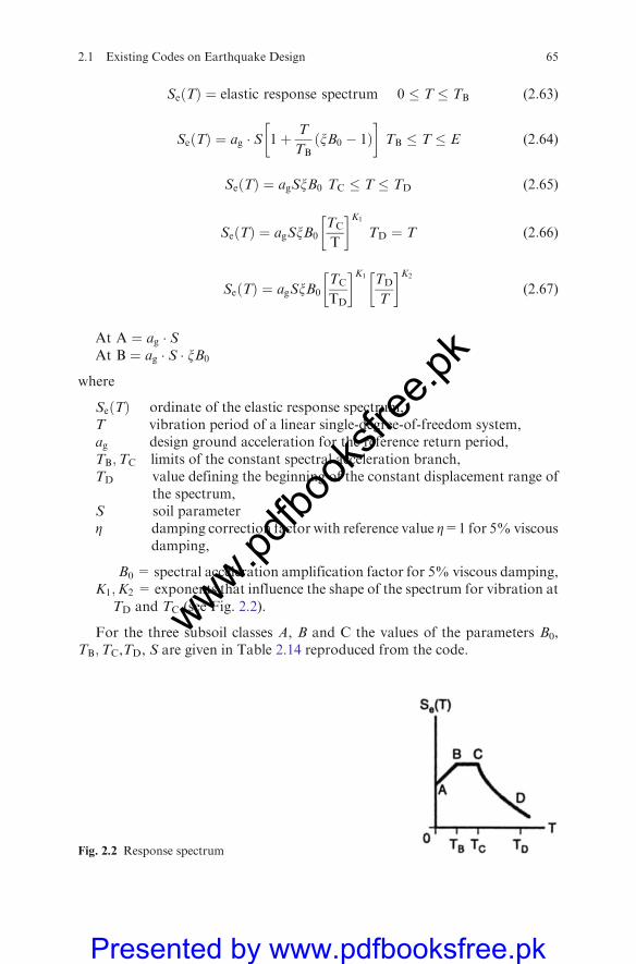
SeðTÞ ¼ elastic response spectrum 0 � T � TB (2:63)
SeðTÞ ¼ ag � S 1þ T
TBðxB0 � 1Þ
� �TB � T � E (2:64)
SeðTÞ ¼ agSxB0 TC � T � TD (2:65)
SeðTÞ ¼ agSxB0TC
T
� �K1
TD ¼ T (2:66)
SeðTÞ ¼ agSxB0TC
TD
� �K1 TD
T
� �K2
(2:67)
At A ¼ ag � SAt B ¼ ag � S � xB0
where
SeðTÞ ordinate of the elastic response spectrum,T vibration period of a linear single-degree-of-freedom system,ag design ground acceleration for the reference return period,TB;TC limits of the constant spectral acceleration branch,TD value defining the beginning of the constant displacement range of
the spectrum,S soil parameterZ damping correction factor with reference value Z=1 for 5% viscous
damping,
B0 = spectral acceleration amplification factor for 5% viscous damping,K1;K2 = exponents that influence the shape of the spectrum for vibration at
TD and TC (see Fig. 2.2).
For the three subsoil classes A, B and C the values of the parameters B0,TB;TC,TD, S are given in Table 2.14 reproduced from the code.
Fig. 2.2 Response spectrum
2.1 Existing Codes on Earthquake Design 65
www.pdfbo
oksfr
ee.pk
Presented by www.pdfbooksfree.pk
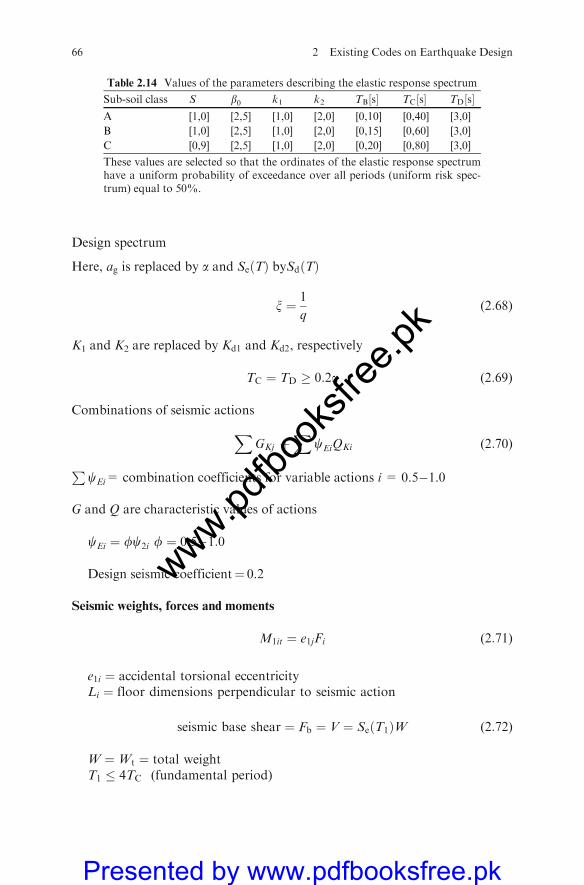
Design spectrum
Here, ag is replaced by a and SeðTÞ bySdðTÞ
x ¼ 1
q(2:68)
K1 and K2 are replaced by Kd1 and Kd2, respectively
TC ¼ TD � 0:2a (2:69)
Combinations of seismic actions
XGKj þ
XcEiQKi (2:70)
PcEi= combination coefficients for variable actions i = 0.5�1.0
G and Q are characteristic values of actions
cEi ¼ fc2i f ¼ 0:5�1:0
Design seismic coefficient¼ 0.2
Seismic weights, forces and moments
M1it ¼ e1jFi (2:71)
e1i ¼ accidental torsional eccentricityLi ¼ floor dimensions perpendicular to seismic action
seismic base shear ¼ Fb ¼ V ¼ SeðT1ÞW (2:72)
W ¼Wt ¼ total weightT1 � 4TC (fundamental period)
Table 2.14 Values of the parameters describing the elastic response spectrum
Sub-soil class S b0 k1 k2 TB½s TC½s TD½sA [1,0] [2,5] [1,0] [2,0] [0,10] [0,40] [3,0]
B [1,0] [2,5] [1,0] [2,0] [0,15] [0,60] [3,0]
C [0,9] [2,5] [1,0] [2,0] [0,20] [0,80] [3,0]
These values are selected so that the ordinates of the elastic response spectrumhave a uniform probability of exceedance over all periods (uniform risk spec-trum) equal to 50%.
66 2 Existing Codes on Earthquake Design
www.pdfbo
oksfr
ee.pk
Presented by www.pdfbooksfree.pk
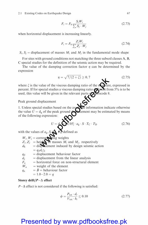
Fi ¼ FbSiWiPSj �Wj
(2:73)
when horizontal displacement is increasing linearly.
Fi ¼ FbZiWiPZj �Wj
(2:74)
Si;Sj ¼ displacement of masses Mi and Mj in the fundamental mode shape
For sites with ground conditions not matching the three subsoil classes A, B,C special studies for the definition of the seismic action may be required.
The value of the damping correction factor Z can be determined by theexpression
Z ¼ffiffiffiffiffiffiffiffiffiffiffiffiffiffiffiffiffiffiffiffi7=ð2þ xÞ
p� 0; 7 (2:75)
where x is the value of the viscous damping ratio of the structure, expressed inpercent. If for special studies a viscous damping ratio different from 5% is to beused, this value will be given in the relevant parts of Eurocode 8.
Peak ground displacement
1. Unless special studies based on the available information indicate otherwisethe value U ¼ dg of the peak ground displacement may be estimated by meansof the following expression:
U ¼ dg ¼ ½0; 05 � ag � S � TC � TD (2:76)
with the values of ag;S;TC;TD defined as
Wi;Wj ¼ corresponding weightsZi;Zj ¼ heights of masses Mi and Mj; respectivelydS ¼ displacement induced by design seismic action
¼ qddegIqd ¼ displacement behaviour factorde ¼ displacement from the linear analysisFa ¼ horizontal force on non-structural elementWa ¼ weight of the elementqa ¼ �B ¼ behaviour factor
¼ 1:0�2:0 ¼ q
Storey drift/P�D effect
P�D effect is not considered if the following is satisfied:
f ¼ Ptot � drVtot � hi
� 0:10 (2:77)
2.1 Existing Codes on Earthquake Design 67
www.pdfbo
oksfr
ee.pk
Presented by www.pdfbooksfree.pk
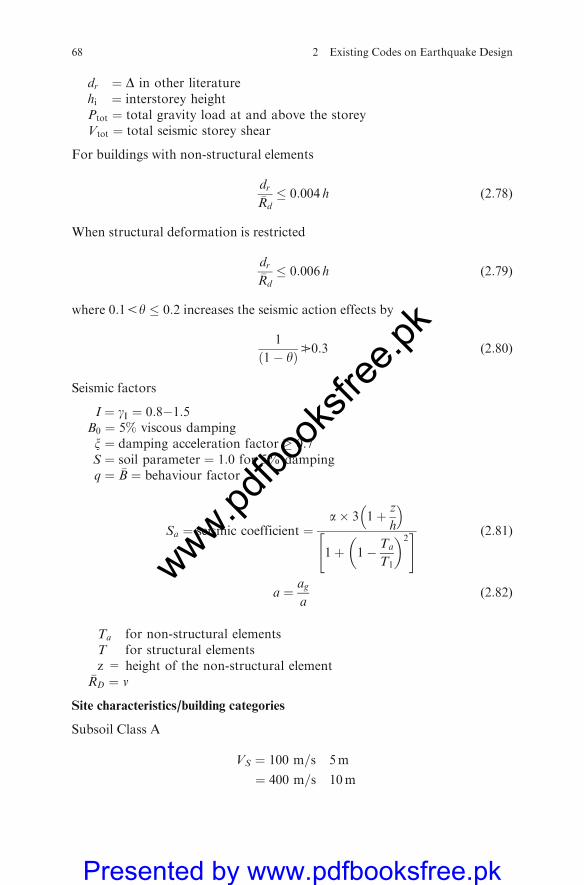
dr ¼ D in other literaturehi ¼ interstorey heightPtot ¼ total gravity load at and above the storeyVtot ¼ total seismic storey shear
For buildings with non-structural elements
dr�Rd
� 0:004 h (2:78)
When structural deformation is restricted
dr�Rd� 0:006 h (2:79)
where 0:15y � 0:2 increases the seismic action effects by
1
ð1� yÞB0:3 (2:80)
Seismic factors
I ¼ gI ¼ 0:8�1:5B0 ¼ 5% viscous dampingx ¼ damping acceleration factor � 0:7S ¼ soil parameter ¼ 1:0 for 5% dampingq ¼ �B ¼ behaviour factor
Sa ¼ seismic coefficient ¼a� 3 1þ z
h
� �
1þ 1� Ta
T1
� �2" # (2:81)
a ¼ ag
a(2:82)
Ta for non-structural elementsT for structural elementsz = height of the non-structural element
�RD ¼ v
Site characteristics/building categories
Subsoil Class A
VS ¼ 100 m=s 5m
¼ 400 m=s 10m
68 2 Existing Codes on Earthquake Design
www.pdfbo
oksfr
ee.pk
Presented by www.pdfbooksfree.pk
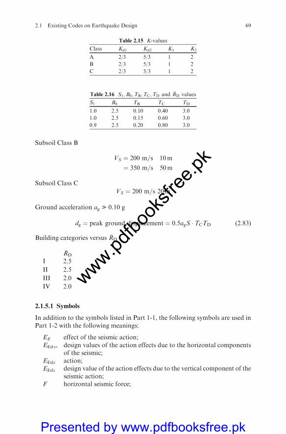
Subsoil Class B
VS ¼ 200 m=s 10m
¼ 350 m=s 50m
Subsoil Class C
VS ¼ 200 m=s 20m
Ground acceleration ag B 0.10 g
dg ¼ peak ground displacement ¼ 0:5agS � TCTD (2:83)
Building categories versus �RD
�RD
I 2.5
II 2.5
III 2.0
IV 2.0
2.1.5.1 Symbols
In addition to the symbols listed in Part 1-1, the following symbols are used inPart 1-2 with the following meanings:
EE effect of the seismic action;EEdx, design values of the action effects due to the horizontal components
of the seismic;EEdy action;EEdz design value of the action effects due to the vertical component of the
seismic action;F horizontal seismic force;
Table 2.16 S1;B0;TB;TC;TD and �RD values
S1 B0 TB TC TD
1.0 2.5 0.10 0.40 3.0
1.0 2.5 0.15 0.60 3.0
0.9 2.5 0.20 0.80 3.0
Table 2.15 K-values
Class Kd1 Kd2 K1 K2
A 2/3 5/3 1 2
B 2/3 5/3 1 2
C 2/3 5/3 1 2
2.1 Existing Codes on Earthquake Design 69
www.pdfbo
oksfr
ee.pk
Presented by www.pdfbooksfree.pk

Fa horizontal seismic force acting on a non-structural element (appendage);H building height;Rd design resistance;T1 fundamental vibration period of a building;Ta fundamental vibration period of a non-structural element
(appendage);W weight;Wa weight of a non-structural element (appendage);d displacement;dr design interstorey drift;e1 accidental eccentricity of a storey mass from its nominal location;h interstorey height;m mass;qa behaviour factor of a non-structural element;qd displacement behaviour factor;s displacement of a mass m in the fundamental mode shape of a
building;z height of the massm above the level of application of the seismic action;ga important factor of a non-structural element;y interstorey drift sensitivity coefficient.
2.1.5.2 Characteristics of Earthquake-Resistant Buildings
Basic Principles of Conceptual Design
(1) P The aspect of seismic hazard shall be taken into consideration in the earlystages of the conceptual design of the building.
(2) The guiding principles governing this conceptual design against seismichazard are– structural simplicity,– uniformity and symmetry,– redundancy,– bidirectional resistance and stiffness,– torsional resistance and stiffness,– diaphragmatic action at storey level,– adequate foundation.
(3) Commentaries to these principles are given in Annex B.
Structural Regularity
General
(1) P For the purpose of seismic design, building structures are distinguished asregular and non-regular.
70 2 Existing Codes on Earthquake Design
www.pdfbo
oksfr
ee.pk
Presented by www.pdfbooksfree.pk

(2) This distinction has implications on the following aspects of the seismicdesign:– method of analysis such as power spectrum, non-linear time history and
frequency domain– the value of the behaviour factor ‘q’– geometric non-linearity exceeding the limit by the Eurocode 8– Non-regular distribution of overstrength in elevation exceeding the limit
by Eurocode 8– Criteria describing regularity in plan and in elevation
Safety Verifications
General
(1) P For the safety verifications the relevant limit states and specific mea-sures (see Clause 2.2.4 of Part 1-1) shall be considered.
(2) For building of importance categories II–IV (see Table 3.3) the verificationsprescribed in Sects. 4.2 and 4.3 may be considered satisfied if the followingtwo conditions are met:
(a) The total base shear due to the seismic design combination (see Clause4.4 of Part 1-1), calculated with a behaviour factor q¼ [1,0], is less thanthat due to the other relevant action combinations for which the build-ing is designed on the basis of a linear elastic analysis.
(b) The specific measures described in Clause 2.2.4 of Part 1-1 of the codeare taken, with the exception that the provisions contained in Clause2.2.4.1 (2)–(3) of Part 1-1 need not be demonstrated as having been met.
Ultimate Limit State
General
(1) P The safety against collapse (ultimate limit state) under the seismic designsituation is considered to be ensured if the following conditions regardingresistance, ductility, equilibrium, foundation stability and seismic joints aremet.
Resistance Condition
(1) P The following relation shall be satisfied for all structural elements –including connections – and the relevant non-structural elements:
Ed � Rd (2:84)
where
Ed ¼ EX
Gkj; gI � AED;PK;X
c2i �Qki
n o
2.1 Existing Codes on Earthquake Design 71
www.pdfbo
oksfr
ee.pk
Presented by www.pdfbooksfree.pk

is the design value of the action effect due to the seismic design situation (see
Clause 4.4 of Part 1-1), including – if necessary – second-order effects, and
Rd ¼ R fk=gMf g (2:85)
is the corresponding design resistance of the element, calculated according
to the rules specific to the pertinent material (characteristic value of prop-
erty fk and partial safety factor gM) and according to the mechanical models
which relate to the specific type of structural system.(2) Second-order effects (P� D effects) need not be considered when the fol-
lowing condition is fulfilled in all storeys:
y ¼ Ptot � drVtot � h
� 0:10 (2:86)
wherey interstorey drift sensitivity coefficient,Ptot total gravity load at and above the storey considered, in accordance
with the assumptions made for the computation of the seismicaction effects,
dr design interstorey drift, evaluated as the difference of the averagelateral displacements at the top and bottom of the storey underconsideration,
Vtot total seismic storey shear,h interstorey height.
(3) In cases when 0:15y � 0:2, the second-order effects can approximately betaken into account by increasing the relevant seismic action effects by afactor equal to 1=ð1 � yÞ.
(4) P The value of the coefficient y shall not exceed 0.3.
Ductility Condition
(1) P It shall be verified that both the structural elements and the structure asa whole possess adequate ductility taking into account the expectedexploration of ductility, which depends on the selected system and thebehaviour factor.
(2) P Specific material-related requirements as defined in Part 1-3 shall besatisfied, including – when indicated – capacity design provisions in order toobtain the hierarchy of resistance of the various structural componentsnecessary for ensuring the intended configuration of plastic hinges and foravoiding brittle failure modes.
(3) P Capacity design rules are presented in detail in Part 1-3.
72 2 Existing Codes on Earthquake Design
www.pdfbo
oksfr
ee.pk
Presented by www.pdfbooksfree.pk

Equilibrium Condition
(1) P The building structure shall be stable under the set of actions given bythe combination rules of Clause 4.4 of Part 1-1. Herein are included sucheffects as overturning and sliding.
(2) P In special cases the equilibrium may be verified by means of energybalance methods or by geometrically non-linear methods with the seismicaction defined as described in Clause 4.3.2 of Part 1-1 of the code.
Resistance of Horizontal Diaphragms
(1) P Diaphragms and bracings in horizontal planes shall be able to transmitwith sufficient overstrength the effects of the design seismic action to thevarious lateral load resisting systems to which they are connected.
(2) Paragraph (1) is considered satisfied if for the relevant resistance verificationsthe forces obtained from the analysis are multiplied by a factor equal to 1.3.
Resistance of Foundations
(1) P The foundation system shall be verified according toClause 5.4 of Part 5and to Eurocode 7.
(2) P The action effects for the foundations shall be derived on the basis ofcapacity design considerations accounting for the development of possibleoverstrength, but they need not exceed the action effects corresponding tothe response of the structure under the seismic design situation inherent tothe assumption of an elastic behaviour (q ¼ 1.0).
(3) If the action effects for the foundation have been determined using abehaviour factor q � ½1; 5, no capacity design considerations accordingto (2) P are required.
Seismic Joint Condition
(1) P Building shall be protected for collisions with adjacent structuresinduced be earthquakes.
(2) Paragraph (1) is deemed to be satisfied if the distance from the boundaryline to the potential points of impact is not less than the maximum hor-izontal displacement.
(3) If the floor elevations of a building under design are the same as those ofthe adjacent building, the above referred distance may be reduced by afactor of [0,7].
(4) Alternatively, this separation distance is not required if appropriate shearwalls are provided on the perimeter of the building to act as collision walls(‘‘bumpers’’). At least two such walls must be placed at each side subject topounding and must extend over the total height of the building. They mustbe perpendicular to the side subject to collisions and they can end on theboundary line. Then the separation distance for the rest of the building canbe reduced to [4,0] cm.
2.1 Existing Codes on Earthquake Design 73
www.pdfbo
oksfr
ee.pk
Presented by www.pdfbooksfree.pk
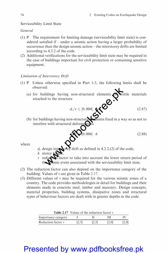
Serviceability Limit State
General
(1) P The requirement for limiting damage (serviceability limit state) is con-sidered satisfied if – under a seismic action having a larger probability ofoccurrence than the design seismic action – the interstorey drifts are limitedaccording to 4.3.2 of the code.
(2) Additional verifications for the serviceability limit state may be required inthe case of buildings important for civil protection or containing sensitiveequipment.
Limitation of Interstorey Drift
(1) P Unless otherwise specified in Part 1-3, the following limits shall beobserved:
(a) for buildings having non-structural elements of brittle materialsattached to the structure
dr=v � ½0; 004 � h (2:87)
(b) for buildings having non-structural elements fixed in a way so as not tointerfere with structural deformations
dr=v � ½0; 006 � h (2:88)
wheredr design interstorey drift as defined in 4.2.2.(2) of the code,h storey height,v reduction factor to take into account the lower return period of
the seismic event associated with the serviceability limit state.
(2) The reduction factor can also depend on the importance category of thebuilding. Values of v are given in Table 2.17.
(3) Different values of v may be required for the various seismic zones of acountry. The code provides methodologies in detail for buildings and theirelements made in concrete steel, timber and masonry. Design concepts,material properties, building systems, dissipative zones and structuraltypes of behaviour factors are dealt with in greater depths in the code.
Table 2.17 Values of the reduction factor v
Importance category I II III IV
Reduction factor v [2,5] [2,5] [2,0] [2,0]
74 2 Existing Codes on Earthquake Design
www.pdfbo
oksfr
ee.pk
Presented by www.pdfbooksfree.pk
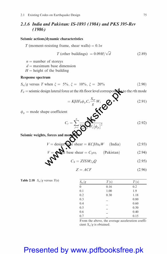
2.1.6 India and Pakistan: IS-1893 (1984) and PKS 395-Rev(1986)
Seismic actions/dynamic characteristics
T (moment-resisting frame, shear walls) ¼ 0:1n
T (other buildings) ¼ 0:09H=ffiffiffidp
(2:89)
n ¼ number of storeysd ¼ maximum base dimensionH ¼ height of the building
Response spectrum
Sa=g versus T when x ¼ 5%; x ¼ 10%; x ¼ 20% ð2:90Þ
Fir¼ seismic design lateral force at the ith floor level corresponding to the rthmode
¼ KbIF0firCrSar
gWi (2:91)
fir ¼ mode shape coefficient
Cr ¼Xnj¼i
WjfjrPnj¼1 Wj fjr
2 (2:92)
Seismic weights, forces and moments
V ¼ design base shear ¼ KCbIa0W ðIndiaÞ (2:93)
V ¼ design base shear ¼ CSot ðPakistanÞ (2:94)
CS ¼ ZISMgdQ (2:95)
Z ¼ ACF (2:96)
Table 2.18 Sa=g versus T(s) Sa=g T ðsÞ T ðsÞ0 0.16 0.2
0.1 1.00 1.9
0.2 0.30 1.18
0.3 _ 0.80
0.4 _ 0.60
0.5 _ 0.50
0.6 _ 0.40
0.7 _ 0.15
From the above, the average acceleration coeffi-cient Sa=g is obtained.
2.1 Existing Codes on Earthquake Design 75
www.pdfbo
oksfr
ee.pk
Presented by www.pdfbooksfree.pk
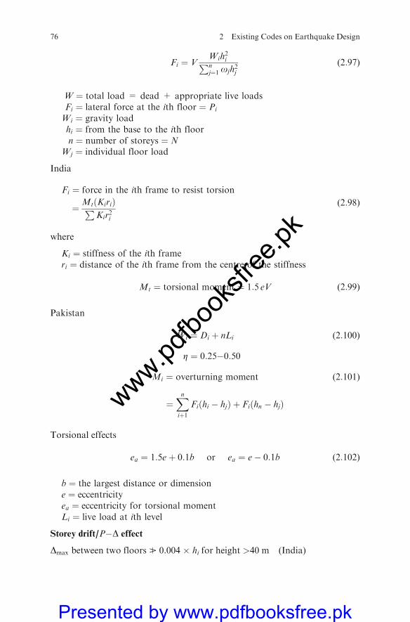
Fi ¼ VWih
2iPn
j¼1 ojh2j
(2:97)
W ¼ total load = dead + appropriate live loadsFi ¼ lateral force at the ith floor ¼ Pi
Wi ¼ gravity loadhi ¼ from the base to the ith floorn ¼ number of storeys ¼ N
Wj ¼ individual floor load
India
Fi ¼ force in the ith frame to resist torsion
¼MtðKiriÞPKir
2i
(2:98)
where
Ki ¼ stiffness of the ith frameri ¼ distance of the ith frame from the centre of the stiffness
Mt ¼ torsional moment ¼ 1:5 eV (2:99)
Pakistan
Wi ¼ Di þ nLi (2:100)
Z ¼ 0:25�0:50
Mi ¼ overturning moment (2:101)
¼Xniþ1
Fiðhi � hjÞ þ Fiðhn � hjÞ
Torsional effects
ea ¼ 1:5eþ 0:1b or ea ¼ e� 0:1b (2:102)
b ¼ the largest distance or dimensione ¼ eccentricityea ¼ eccentricity for torsional momentLi ¼ live load at ith level
Storey drift/P�D effect
Dmax between two floors B 0.004 � hi for height >40 m (India)
76 2 Existing Codes on Earthquake Design
www.pdfbo
oksfr
ee.pk
Presented by www.pdfbooksfree.pk
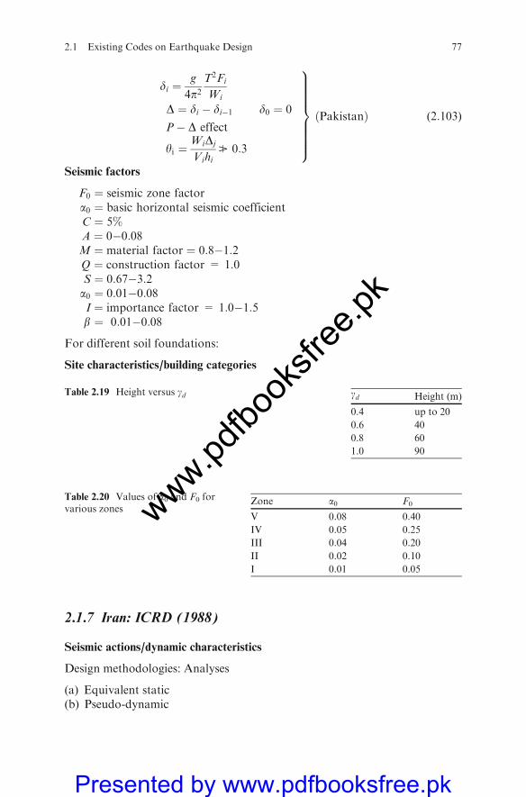
di ¼g
4p2T2Fi
Wi
D ¼ di � di�1 d0 ¼ 0
P� D effect
yi ¼WiDj
VihiB 0:3
9>>>>>>>=>>>>>>>;ðPakistanÞ (2:103)
Seismic factors
F0 ¼ seismic zone factora0 ¼ basic horizontal seismic coefficientC ¼ 5%A ¼ 0�0:08M ¼ material factor ¼ 0:8�1:2Q ¼ construction factor = 1:0S ¼ 0:67�3:2a0 ¼ 0:01�0:08I ¼ importance factor = 1:0�1:5b ¼ 0:01�0:08
For different soil foundations:
Site characteristics/building categories
2.1.7 Iran: ICRD (1988)
Seismic actions/dynamic characteristics
Design methodologies: Analyses
(a) Equivalent static(b) Pseudo-dynamic
Table 2.20 Values of a0 and F0 forvarious zones
Zone a0 F0
V 0.08 0.40
IV 0.05 0.25
III 0.04 0.20
II 0.02 0.10
I 0.01 0.05
Table 2.19 Height versus gd gd Height (m)
0.4 up to 20
0.6 40
0.8 60
1.0 90
2.1 Existing Codes on Earthquake Design 77
www.pdfbo
oksfr
ee.pk
Presented by www.pdfbooksfree.pk
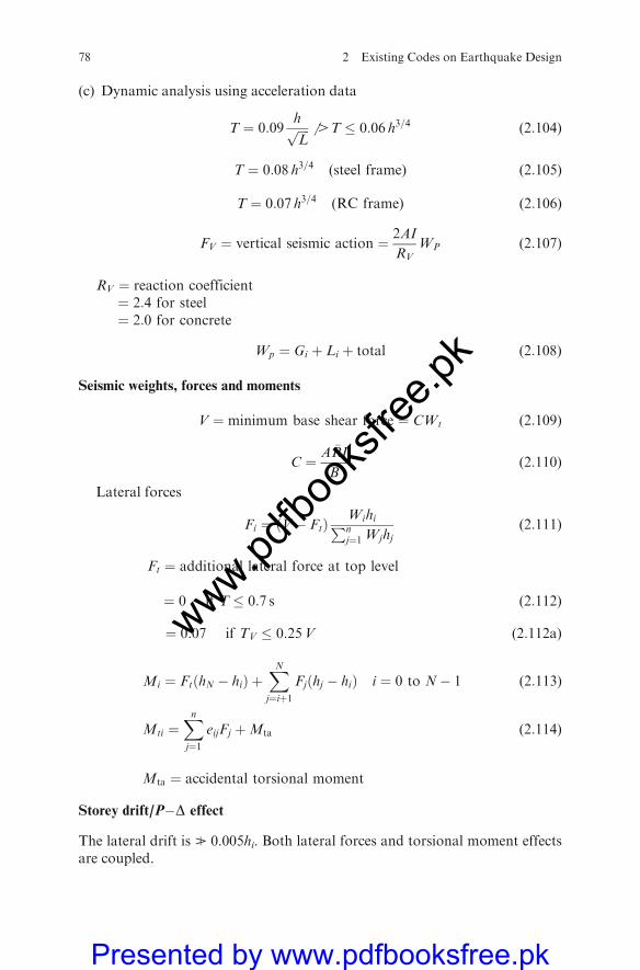
(c) Dynamic analysis using acceleration data
T ¼ 0:09hffiffiffiffiLp 64T � 0:06 h3=4 (2:104)
T ¼ 0:08 h3=4 (steel frame) (2:105)
T ¼ 0:07 h3=4 (RC frame) (2:106)
FV ¼ vertical seismic action ¼ 2AI
RVWP (2:107)
RV ¼ reaction coefficient¼ 2:4 for steel¼ 2:0 for concrete
Wp ¼ Gi þ Li þ total (2:108)
Seismic weights, forces and moments
V ¼ minimum base shear force ¼ CWt (2:109)
C ¼ A �RI�B
(2:110)
Lateral forces
Fi ¼ ðV� FtÞWihiPnj¼1Wjhj
(2:111)
Ft ¼ additional lateral force at top level
¼ 0 if T � 0:7 s (2:112)
¼ 0:07 if TV � 0:25V (2:112a)
Mi ¼ FtðhN � hiÞ þXNj¼iþ1
Fjðhj � hiÞ i ¼ 0 to N� 1 (2:113)
Mti ¼Xnj¼1
eijFj þMta (2:114)
Mta ¼ accidental torsional moment
Storey drift/P�D effect
The lateral drift is B 0.005hi. Both lateral forces and torsional moment effectsare coupled.
78 2 Existing Codes on Earthquake Design
www.pdfbo
oksfr
ee.pk
Presented by www.pdfbooksfree.pk
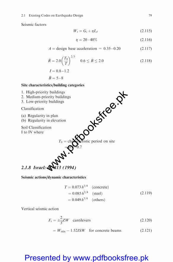
Seismic factors
Wt ¼ Gi þ ZLI (2:115)
Z ¼ 20�40% (2:116)
A ¼ design base acceleration = 0:35�0:20 (2:117)
�R ¼ 2:0T0
T
� �2=3
0:6 � �R � 2:0 (2:118)
I ¼ 0.8�1.2�B ¼ 5�8
Site characteristics/building categories
1. High-priority buildings2. Medium-priority buildings3. Low-priority buildings
Classification
(a) Regularity in plan(b) Regularity in elevation
Soil ClassificationI to IV where
T0 ¼ characteristic period on site
¼ 0:3�0:7
2.1.8 Israel: IC-413 (1994)
Seismic actions/dynamic characteristics
T ¼ 0:073 h3=4 concreteð Þ¼ 0:085 h3=4 steelð Þ¼ 0:049 h3=4 othersð Þ
(2:119)
Vertical seismic action
Fr ¼ �2
3ZW cantilevers (2:120)
¼Wmin � 1:52ISW for concrete beams (2:121)
2.1 Existing Codes on Earthquake Design 79
www.pdfbo
oksfr
ee.pk
Presented by www.pdfbooksfree.pk
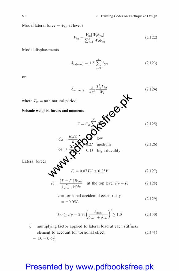
Modal lateral force = Fim at level i
Fim ¼Vm Wifim½ Pn
i¼1 Wifim
(2:122)
Modal displacements
dim maxð Þ ¼ �KXij¼0
Djm (2:123)
or
dim maxð Þ ¼g
4p2T2mFim
Wi(2:124)
where Tm ¼ mth natural period.
Seismic weights, forces and moments
V ¼ Cd
XNi¼1
Wi (2:125)
Cd ¼RaIZ
�R
or � SIZffiffiffiffiffiffi3 �Rp
9>>=>>;B
0:3I low
0:2I medium
0:1I high ductility
(2:126)
Lateral forces
Ft ¼ 0:07TV � 0:25V (2:127)
Fi ¼V� Ftð ÞWihiPN
i ¼ 1 Wihiat the top level FN þ Ft (2:128)
e ¼ torsional accidental eccentricity
¼ �0:05L(2:129)
3:0 � AT ¼ 2:75dmax
dmax þ dmin
� �2
� 1:0 (2:130)
x ¼ multiplying factor applied to lateral load at each stiffness
element to account for torsional effect
¼ 1:0þ 0:6 yL
(2:131)
80 2 Existing Codes on Earthquake Design
www.pdfbo
oksfr
ee.pk
Presented by www.pdfbooksfree.pk
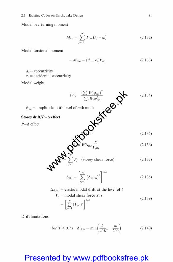
Modal overturning moment
Mim ¼XNj¼iþ1
Fpm hj � hi �
(2:132)
Modal torsional moment
¼Mtim ¼ di � eið ÞVim (2:133)
di ¼ eccentricityei ¼ accidental eccentricity
Modal weight
Wm ¼P
iWifimð Þ2PiWif2
im
(2:134)
fim= amplitude at ith level of mth mode
Storey drift/P�D effect
P�D effect
yi41:0 (2:135)
yi ¼WDel;iK
Vihi(2:136)
Vi ¼XNj¼i
Fj storey shear forceð Þ (2:137)
Del;i ¼XNm¼1
Del; im
�2" #1=2(2:138)
Del; im ¼ elastic modal drift at the level of i
Vi ¼ modal shear force at i
¼PNm¼1
Vimð Þ2� �1=2 (2:139)
Drift limitations
for T � 0:7 s Di;lim ¼ minhi40K
;hi200
� �(2:140)
2.1 Existing Codes on Earthquake Design 81
www.pdfbo
oksfr
ee.pk
Presented by www.pdfbooksfree.pk
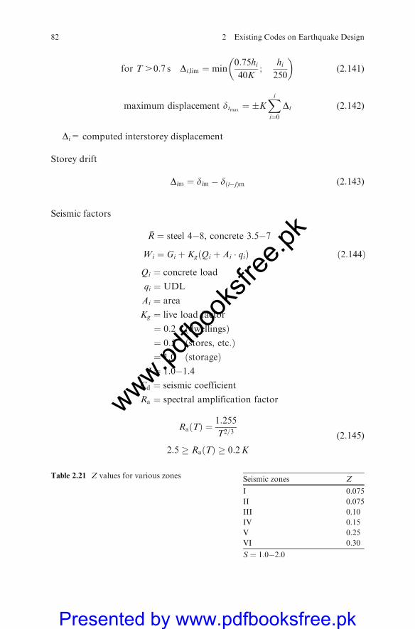
for T40:7 s Di;lim ¼ min0:75hi40K
;hi250
� �(2:141)
maximum displacement dtmax¼ �K
Xii¼0
Di (2:142)
Di= computed interstorey displacement
Storey drift
Dim ¼ dim � d i�jð Þm (2:143)
Seismic factors
�R ¼ steel 4�8, concrete 3:5�7
Wi ¼ Gi þ Kg Qi þ Ai � qið Þ ð2:144Þ
Qi ¼ concrete load
qi ¼ UDL
Ai ¼ area
Kg ¼ live load factor
¼ 0:2 dwellingsð Þ¼ 0:5 stores, etc:ð Þ¼ 1:0 storageð Þ
I ¼ 1:0�1:4Cd ¼ seismic coefficient
Ra ¼ spectral amplification factor
Ra Tð Þ ¼ 1:255
T2=3
2:5 � Ra Tð Þ � 0:2K
(2:145)
Table 2.21 Z values for various zones Seismic zones Z
I 0.075
II 0.075
III 0.10
IV 0.15
V 0.25
VI 0.30
S ¼ 1:0�2:0
82 2 Existing Codes on Earthquake Design
www.pdfbo
oksfr
ee.pk
Presented by www.pdfbooksfree.pk

Site characteristics/building categories
Regular structuresCategory B580m highCategory C580m high
with normalized seismic zones Z � 0:075:
2.1.9 Italy: CNR-GNDT (1986) and Eurocode EC8is Implemented
Seismic actions/dynamic characteristics
Seismic index S = 6, 9 and 12Fundamental period T0
T040:8 s �R ¼ 0:862=T2=30 (2:146)
T0 � 0:8 s �R ¼ 1:0 (2:147)
T0 ¼ 0:1hffiffiffiffiLp for a framed structure (2:148)
Lateral and vertical effects
a ¼ a2h þ a2v 1=2
(2:149)
�Z ¼ Z2h þ Z2v 1=2
(2:150)
a ¼ single force componenth; v ¼ subscripts for horizontal and verticalZ ¼ single displacement component
Combination of modal effects
a ¼ffiffiffiffiffiffiffiffiffiffiffiffiffiXa
a2ir
(2:151)
Structure Maximum height (m)
Frame S ¼ 6 S ¼ 9 S ¼ 12
Frame No limitation
Masonry 16.0 11.0 7.5
Walls 32.0 25.0 15.0
Timber 10.0 7.0 7.0
2.1 Existing Codes on Earthquake Design 83
www.pdfbo
oksfr
ee.pk
Presented by www.pdfbooksfree.pk
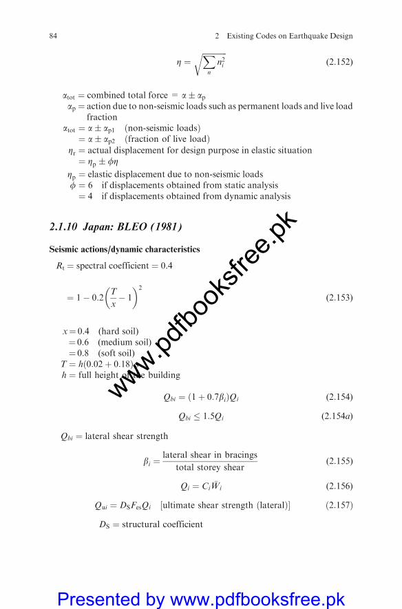
Z ¼ffiffiffiffiffiffiffiffiffiffiffiffiffiXn
n2i
r(2:152)
atot ¼ combined total force = a� apap ¼ action due to non-seismic loads such as permanent loads and live load
fractionatot ¼ a� ap1 non-seismic loadsð Þ¼ a� ap2 fraction of live loadð Þ
Zr ¼ actual displacement for design purpose in elastic situation¼ Zp � fZ
Zp ¼ elastic displacement due to non-seismic loadsf ¼ 6 if displacements obtained from static analysis¼ 4 if displacements obtained from dynamic analysis
2.1.10 Japan: BLEO (1981)
Seismic actions/dynamic characteristics
Rt ¼ spectral coefficient ¼ 0.4
¼ 1� 0:2T
x� 1
� �2
(2:153)
x¼ 0.4 (hard soil)¼ 0.6 (medium soil)¼ 0.8 (soft soil)
T ¼ h 0:02þ 0:18ð Þ sh ¼ full height of the building
Qbi ¼ 1þ 0:7bið ÞQi (2:154)
Qbi � 1:5Qi (2:154a)
Qbi ¼ lateral shear strength
bi ¼lateral shear in bracings
total storey shear(2:155)
Qi ¼ Ci�Wi (2:156)
Qui ¼ DSFesQi ultimate shear strength lateralð Þ½ ð2:157Þ
DS ¼ structural coefficient
84 2 Existing Codes on Earthquake Design
www.pdfbo
oksfr
ee.pk
Presented by www.pdfbooksfree.pk
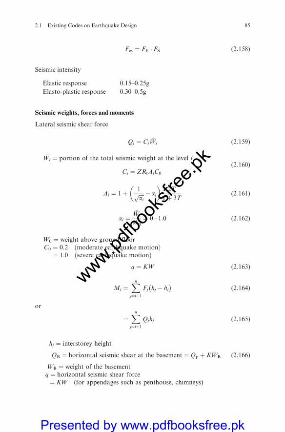
Fes ¼ FE � FS (2:158)
Seismic intensity
Seismic weights, forces and moments
Lateral seismic shear force
Qi ¼ Ci�Wi (2:159)
�Wi ¼ portion of the total seismic weight at the level i
Ci ¼ ZRtAiC0
(2:160)
Ai ¼ 1þ 1ffiffiffiffiaip � ai
� �2T
1þ 3T(2:161)
ai ¼�Wi
W0¼ 0�1:0 (2:162)
W0 ¼ weight above ground floorC0 ¼ 0:2 moderate earthquake motionð Þ¼ 1:0 severe earthquake motionð Þ
q ¼ KW (2:163)
Mi ¼Xnj¼iþ1
Fj hj � hi �
(2:164)
or
¼Xnj¼iþ1
Qjhj (2:165)
hj ¼ interstorey height
QB ¼ horizontal seismic shear at the basement ¼ Qp þ KWB (2:166)
WB ¼ weight of the basementq ¼ horizontal seismic shear force¼ KW (for appendages such as penthouse, chimneys)
Elastic response 0.15–0.25g
Elasto-plastic response 0.30–0.5g
2.1 Existing Codes on Earthquake Design 85
www.pdfbo
oksfr
ee.pk
Presented by www.pdfbooksfree.pk
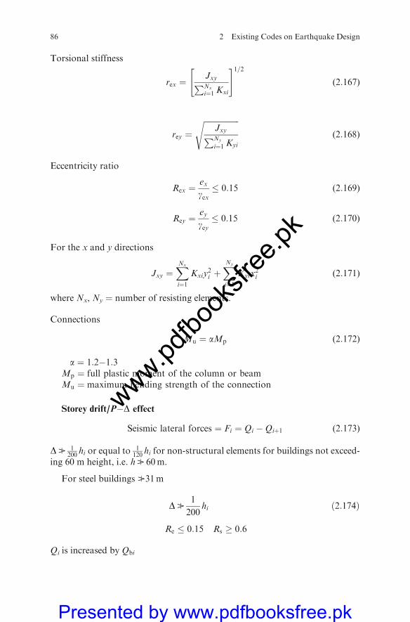
Torsional stiffness
rex ¼JxyPNx
i¼1Kxi
" #1=2(2:167)
rey ¼ffiffiffiffiffiffiffiffiffiffiffiffiffiffiffiffiffiffi
JxyPNy
i¼1 Kyi
s(2:168)
Eccentricity ratio
Rex ¼exgex� 0:15 (2:169)
Rey ¼ey
gey� 0:15 (2:170)
For the x and y directions
Jxy ¼XNx
i¼1Kxiy
2i þ
XNy
i¼1Kyix
2i (2:171)
where Nx, Ny ¼ number of resisting elements.
Connections
Mu ¼ aMp (2:172)
a ¼ 1:2�1:3Mp ¼ full plastic moment of the column or beamMu ¼ maximum bending strength of the connection
Storey drift/P�D effect
Seismic lateral forces ¼ Fi ¼ Qi �Qiþ1 (2:173)
DB 1200
hi or equal to1120
hi for non-structural elements for buildings not exceed-ing 60 m height, i.e. hB 60m.
For steel buildings B31m
DB1
200hi ð2:174Þ
Re � 0:15 Rs � 0:6
Qi is increased by Qbi
86 2 Existing Codes on Earthquake Design
www.pdfbo
oksfr
ee.pk
Presented by www.pdfbooksfree.pk
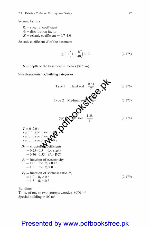
Seismic factors
Rt ¼ spectral coefficientAi ¼ distribution factorZ ¼ seismic coefficient ¼ 0.7–1.0
Seismic coefficient K of the basement
� 0:1 1� H
40
� �� Z (2:175)
H ¼ depth of the basement in metres ðB20mÞ.
Site characteristics/building categories
Type 1 Hard soil0:64
T(2:176)
Type 2 Medium soil0:96
T(2:177)
Type 3 Soft soil1:28
T(2:178)
T ¼ 0–2.0 sTC for Type 1 soil ¼ 0.4TC for Type 2 soil ¼ 0.6TC for Type 3 soil ¼ 0.8
DS ¼ structural coefficients¼ 0:25�0:5 for steelð Þ¼ 0:30�0:55 for RCð Þ
Fe ¼ function of eccentricity¼ 1:0 for Re50:15¼ 1:5 for Re40:3
FS ¼ function of stiffness ratio Rx
¼ 1:0 RS40:6¼ 1:5 RS50:3
(2:179)
BuildingsThose of one to two-storeys: wooden B500m2
Special building B100m2
2.1 Existing Codes on Earthquake Design 87
www.pdfbo
oksfr
ee.pk
Presented by www.pdfbooksfree.pk

RC buildings
25X
AW þ 7X
AC � Z �WiAi for hB 20 m (2:180)
25X
AW þ 7X
AC þ 10X
A0C � 0:75ZAi�Wi for hB 31 m (2:181)
Steel buildings
(1) Not exceeding three storeysh � 13 m span � 6 mtotal floor area � 500 m2
C0 ¼ 0:3(2) Not exceeding 60 m
Qui � Qu (2:182)
PAC ¼ summation of total column areasPAW ¼ summation of total horizontal cross-sectional areas of walls
2.1.11 Mexico: UNAM (1983) M III (1988)
Seismic actions/dynamic characteristics
T0 ¼ 4Xi
ti
bli(2:183)
Design spectraReferring to Fig. 2.3:
a ¼ 1þ 3T
Ta
� �C
4for T � Ta s (2:184)
a ¼ C for Ta5T � Tb s (2:185)
a ¼ Tb
T
� �r
c for T4Tb s (2:186)
T reduced lateral forcesð Þ ¼ 0:63XNi¼1
Wix2i
gPN
i¼1 Fixi
!1=2
(2:187)
x ¼ displacementsFi ¼ force at ith levela ¼ spectral acceleration
88 2 Existing Codes on Earthquake Design
www.pdfbo
oksfr
ee.pk
Presented by www.pdfbooksfree.pk
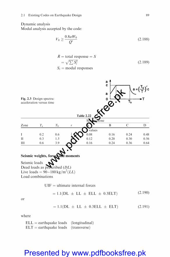
Dynamic analysisModal analysis accepted by the code:
V0 �0:8aW0
Q0(2:188)
�R ¼ total response ¼ S
¼ffiffiffiffiffiffiffiffiffiffiffiP
S2i
pSi ¼ modal responses
(2:189)
Seismic weights, forces and moments
Seismic loadsDead loads as prescribed (DL)Live loads ¼ 90�180 kg=m2 LLð ÞLoad combinations
UIF ¼ ultimate internal forces
¼ 1:1 DL � LL � ELL � 0:3ELTð Þ (2:190)
or
¼ 1:1 DL � LL � 0:3ELL � ELTð Þ (2:191)
where
ELL ¼ earthquake loads longitudinalð ÞELT ¼ earthquake loads transverseð Þ
Fig. 2.3 Design spectra:acceleration versus time
Table 2.22
Seismic zone
Zone Ta Tb r A B C D
c values
I 0.2 0.6 12
0.08 0.16 0.24 0.48
II 0.3 1.5 23 0.12 0.20 0.30 0.56
III 0.6 3.9 1.0 0.16 0.24 0.36 0.64
2.1 Existing Codes on Earthquake Design 89
www.pdfbo
oksfr
ee.pk
Presented by www.pdfbooksfree.pk
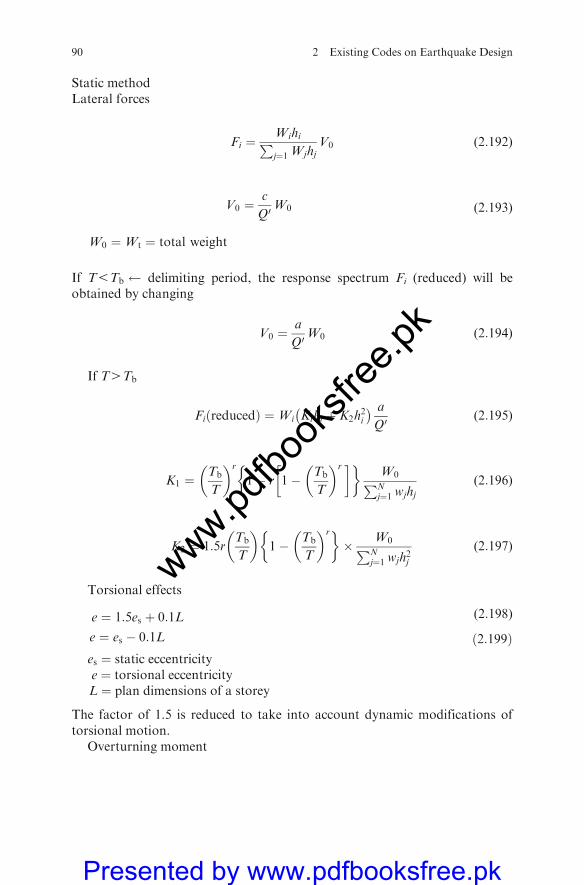
Static methodLateral forces
Fi ¼WihiPj¼1 Wjhj
V0 (2:192)
V0 ¼c
Q0W0
W0 ¼Wt ¼ total weight
(2:193)
If T5Tb delimiting period, the response spectrum Fi (reduced) will beobtained by changing
V0 ¼a
Q0W0 (2:194)
If T4Tb
Fi reducedð Þ ¼Wi Kihi þ K2h2i
� a
Q0(2:195)
K1 ¼Tb
T
� �r
1� r 1� Tb
T
� �r� �� �W0PNj¼1 wjhj
(2:196)
K2 ¼ 1:5rTb
T
� �1� Tb
T
� �r� �� W0PN
j¼1 wjh2j
(2:197)
Torsional effects
e ¼ 1:5es þ 0:1L
e ¼ es � 0:1L ð2:199Þ
(2:198)
es ¼ static eccentricitye ¼ torsional eccentricityL ¼ plan dimensions of a storey
The factor of 1.5 is reduced to take into account dynamic modifications oftorsional motion.
Overturning moment
90 2 Existing Codes on Earthquake Design
www.pdfbo
oksfr
ee.pk
Presented by www.pdfbooksfree.pk
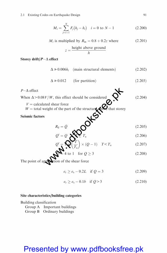
Mi ¼XNj¼iþ1
Fj hj � hi �
i ¼ 0 to N� 1 (2:200)
Mi is multiplied by Rm ¼ 0:8þ 0:2z where
z ¼ height above ground
h
(2:201)
Storey drift/P�D effect
DB 0:006hi main structural elementsð Þ
DB 0:012 for partitionð Þ ð2:203Þ
(2:202)
P�D effect
When D40:08V=W, this effect should be considered (2:204)
V ¼ calculated shear forceW ¼ total weight of the part of the structure above that storey
Seismic factors
Rd ¼ �Q (2:205)
Q0 ¼ Q T � Ta (2:206)
Q0 ¼ 1þ T
Ta
� �� Q� 1ð Þ T5Ta (2:207)
Q ¼ 4 to 1 for Q � 3 (2:208)
The point of application of the shear force
er � es � 0:2L if Q ¼ 3 (2:209)
er � es � 0:1b if Q43 (2:210)
Site characteristics/building categories
Building classificationGroup A Important buildingsGroup B Ordinary buildings
2.1 Existing Codes on Earthquake Design 91
www.pdfbo
oksfr
ee.pk
Presented by www.pdfbooksfree.pk

sands > 50 m
bi ¼P
i tiPitibli
(2:211)
ti ¼ thickness of soil layers iGi ¼ shear modulus tons/m2
gi ¼ unit weight tons/m3
b1 ¼ffiffiffiffiffigGi
gi
qfor Class II
b15700�550T0 ð2:213Þ(2:212)
For outside Mexico
a ¼ a0 þ c� a0ð Þ TTa
for T � Ta (2:214)
2.1.12 New Zealand: NZS 4203 (1992) and NZNSEE (1988)
Seismic actions/dynamic characteristics
Methods
(a) Equivalent static method(b) Modal response spectrum(c) Numerical integration time – history analysis
T ¼ 2pPN
i¼1 Wiu2iPN
i¼1 Wiui
" #1=2(2:215)
T ¼ 0:042 (2:216)
ui ¼ 1:0 for one storey¼ 0:85 for six or more storeys¼ for fewer than six storeys interpolate between 1:0 and 0:85
ui ¼ lateral displacement at level idt ¼ lateral displacement in millimetres at the top of the building
Table 2.23 Seismic zones: soil types
Seismic zones Soil types
I Hill zone, stiff rock, soft clays
II Transition zone, sandy, silty sands < 20 m
III Lake bed zone, clays, silty clay
92 2 Existing Codes on Earthquake Design
www.pdfbo
oksfr
ee.pk
Presented by www.pdfbooksfree.pk
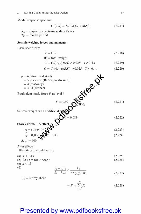
Modal response spectrum
C1 Tmð Þ ¼ SmCb Tm; 1ð Þ �RZfL (2:217)
Sm ¼ response spectrum scaling factorTm ¼ modal period
Seismic weights, forces and moments
Basic shear force
V ¼ CW
W ¼ total weight
(2:218)
C ¼ Cb T; mð Þ �RZfL40:025 T40:4 s (2:219)
C ¼ Cb 0:4; mð ÞRZfL40:025 T � 0:4 s (2:220)
m ¼ 6 (structural steel)¼ 5 [concrete (RC or prestressed)]¼ 4 (masonry)¼ 3�4 (timber)
Equivalent static force Fi at level i
Fi ¼ 0:92VWihiPNj¼1Wjhj
(2:221)
Seismic weight with additional top force
Ft ¼ 0:08V (2:222)
Storey drift/P�D effect
D ¼ storey drift ð2:223ÞDh
0; 0:2; 0:4; 0:6 %ð Þ ð2:224ÞDmax ¼ 600
P�D effectsUltimately it should satisfy
(a) T50:4 s ð2:225Þ(b) hB15m for T50:8 s ð2:226Þ(c) m51:5(d) ui � ui�1
hi � hi�1� Vi
7:5PN
j¼1 Wi
Vi ¼ storey shear
(2:227)
¼ Ft þXNi¼1
Fj (2:228)
2.1 Existing Codes on Earthquake Design 93
www.pdfbo
oksfr
ee.pk
Presented by www.pdfbooksfree.pk
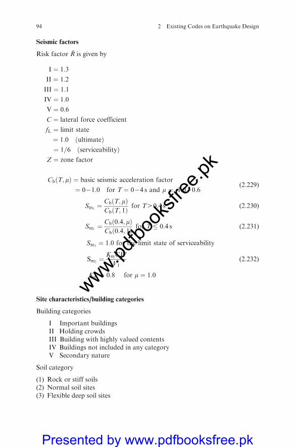
Seismic factors
Risk factor �R is given by
I ¼ 1:3
II ¼ 1:2
III ¼ 1:1
IV ¼ 1:0
V ¼ 0:6
C ¼ lateral force coefficient
fL ¼ limit state
¼ 1:0 ultimateð Þ¼ 1=6 ðserviceabilityÞ
Z ¼ zone factor
Cb T; mð Þ ¼ basic seismic acceleration factor
¼ 0�1:0 for T ¼ 0�4 s and m ¼ 1:0�0:6(2:229)
Sm1¼ Cb T; mð Þ
Cb T; 1ð Þ for T40:4 s (2:230)
Sm1¼ Cb 0:4; mð Þ
Cb 0:4; 1ð Þ for T � 0:4 s (2:231)
Sm1¼ 1:0 for the limit state of serviceability
Sm2¼ KmCW
V1(2:232)
Km ¼ 0:8 for m ¼ 1:0
Site characteristics/building categories
Building categories
I Important buildingsII Holding crowdsIII Building with highly valued contentsIV Buildings not included in any categoryV Secondary nature
Soil category
(1) Rock or stiff soils(2) Normal soil sites(3) Flexible deep soil sites
94 2 Existing Codes on Earthquake Design
www.pdfbo
oksfr
ee.pk
Presented by www.pdfbooksfree.pk
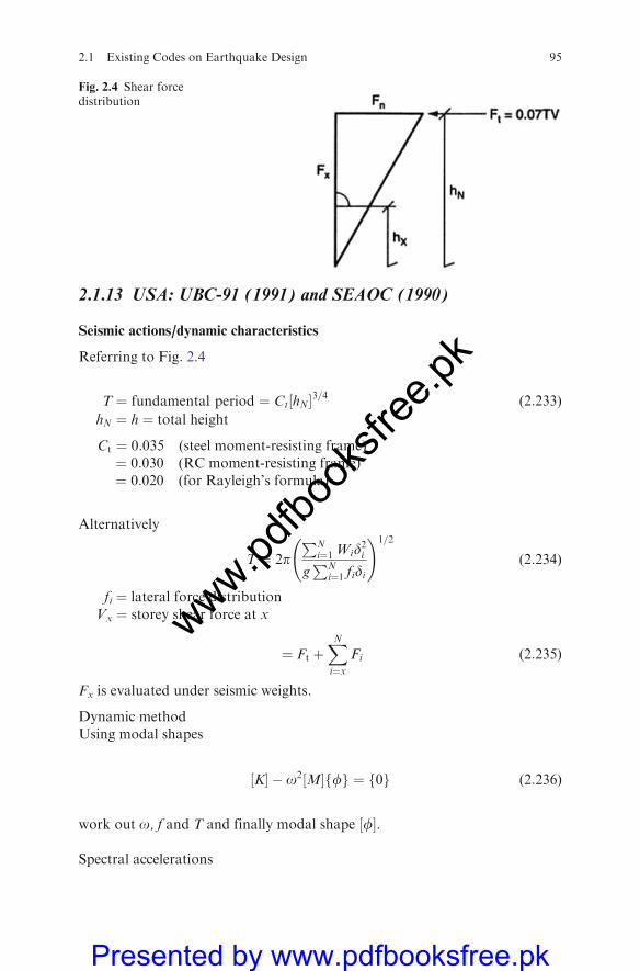
2.1.13 USA: UBC-91 (1991) and SEAOC (1990)
Seismic actions/dynamic characteristics
Referring to Fig. 2.4
T ¼ fundamental period ¼ Ct hN½ 3=4 (2:233)
hN ¼ h ¼ total height
Ct ¼ 0:035 (steel moment-resisting frame)¼ 0:030 (RC moment-resisting frame)¼ 0:020 (for Rayleigh’s formula)
Alternatively
T ¼ 2pPN
i¼1 Wid2igPN
i¼1 fidi
!1=2
(2:234)
fi ¼ lateral force distributionVx ¼ storey shear force at x
¼ Ft þXNi¼x
Fi (2:235)
Fx is evaluated under seismic weights.
Dynamic methodUsing modal shapes
K½ � o2 M½ ff g ¼ 0f g (2:236)
work out o, f and T and finally modal shape f½ .
Spectral accelerations
Fig. 2.4 Shear forcedistribution
2.1 Existing Codes on Earthquake Design 95
www.pdfbo
oksfr
ee.pk
Presented by www.pdfbooksfree.pk
Scaled down by peak one of 0:3g=Rw ¼ 12:
Sa1 ¼ 0:034g Sa2 ¼ 0:063g (2:237)
Sa3 ¼ 0:061g Sa4 ¼ 0:05g (2:238)
Seismic weights, forces and moments
V ¼ basic shear force ¼ ZICW
Rw(2:239)
C ¼ 1:25S
T2=3� 2:75 (2:240)
Rw ¼ structural factor ¼ 4–12
Fx ¼V� Ftð ÞWxhxPN
i¼1 Wihiat level x from the base (2:241)
Ft ¼ 0:07TV � 0:25V for T40:7 s (2:242)
Ft ¼ 0 for T � 0:7 s
V ¼ Ft þXNi¼1
Fi (2:243)
Storey shear force
Vx ¼ Ft þXNi¼x
Fi (2:244)
Mx ¼ overturning moment, thus
Mx ¼ Ft hN � hxð Þ þXNi¼xþ1
Fi hi � hxð Þ where x ¼ 0; 1; 2; . . . ;N� 1 (2:245)
Torsional momentTorsional (based on UBC-91) irregularities in buildings are considered byincreasing the accidental torsion by Ax (amplification factor)
Ax ¼dmax at x
1:20davg
� �2
� 3:0 (2:246)
davg ¼ the average displacement at extreme points at level x.
96 2 Existing Codes on Earthquake Design
www.pdfbo
oksfr
ee.pk
Presented by www.pdfbooksfree.pk
The floor and the roof diaphragms shall resist the forces determined by thefollowing formula:
Fpx ¼Ft þ
PNi¼x FiPN
i¼x Wi
Wpx (2:247)
whereWpx ¼ weight of the diaphragm and attached parts of the building.
Correspondingly FpxB0:75ZIWpx and C 0:35ZIWpx (2:248)
Storey drift/P�D effect
Drift calculated B0:04
Rw� hi (2:249)
or B0:005hi for T50:7 s
or B0:004hi for T � 0:7 s
P�D effectSecondary moment formula driftPrimary moment due to lateral forces
Mxs
MspB0:10 not considered for greater values (2:250)
yx ¼Mxs
Msp¼ PxDx
VxHx(2:251)
Subscript x means to the level of storey x.
Elastic storey drift
Die ¼Vi
Ki(2:252)
Di ¼ inelastic storey drift
¼ Die
KK51:0ð Þ (2:253)
or
Di ¼ RDie (2:254)
di ¼ lateral displacement ¼XNi¼1
Di (2:255)
2.1 Existing Codes on Earthquake Design 97
www.pdfbo
oksfr
ee.pk
Presented by www.pdfbooksfree.pk
Total displacement
dpx ¼ dix � yYp (2:256)
dpy ¼ diy þ yYp (2:257)
dix; diy ¼ lateral displacement in x and y directionsy ¼ storey rotation
dpx; dpy ¼ lateral displacement in x and y directionsdp ¼ total displacement at a selected point P¼ d2px þ d2py
�1=2Seismic factors
Z ¼ seismic zone factorZ ¼ 0:075 Zone I¼ 0:15 Zone IIA¼ 0:20 Zone IIB¼ 0:30 Zone III¼ 0:40 Zone IV
I ¼ occupancy or importance factor ¼ 1:0�1:25
Site characteristics/building categories
S1 type
Sa ¼ 1þ 10T 05T � 0:15 s (2:258)
Sa ¼ 2:5T 0:155T � 0:39 s (2:259)
Sa ¼0:975
TT40:39 s (2:260)
S2 type
Sa ¼ 1þ 10T 05T � 0:15 sð2:261ÞSa ¼ 2:5T 0:155T � 0:585 sð2:262Þ
(2:261)
Table 2.24 Soils in seismic zones
Seismic zones Soil S*
I Rock like 1.0 (S1)
IIA Dense stiff 1.2 (S2)
IIB
II Soft-medium clay 1.5 (S3)
IV Soft clay 2.0 (S4)
S*= site coefficient
98 2 Existing Codes on Earthquake Design
www.pdfbo
oksfr
ee.pk
Presented by www.pdfbooksfree.pk
Sa ¼1:463
TT40:585 s (2:262)
S3 type
Sa ¼ 1þ 75T 05T � 0:2 s (2:263)
Sa ¼ 2:5T 0:25T � 0:915 s (2:264)
Sa ¼2:288
TT T40:915 s (2:265)
K ¼ spring parameter of the damperC ¼ viscous constant of the dampera ¼ parameter of the damper, a usually varies between 0.1 and 0.4
Parameters should be experimentally calibrated by the supplier.
Additional deliberations on viscoelastic dampers
A convenient way to improve the dynamic performance of a structure sub-jected to wind or earthquake loading vibration is to incorporate mechanicaldampers to augment the structural damping. This damping increase yields areduction in the expected structural damage through a significant reduction ofthe interstory drifts of the structure during the dynamic event.
Although the developments in research and analysis techniques, paralleledby significant improvements and refinements of device hardware, make themechanical dampers totally suitable for consideration in new or retrofit design,there are still relatively few applications to buildings (Mahmoodi 1969; Aikenand Kelly 1990; Tsai and Lee 1993; Inaudi et al. 1993; Inaudi and Kelly 1995;Lai et al. 1995; Shen and Soong 1995; Makri et al. 1995).
Among a number of viable types of energy dissipation devices proposed, theviscoelastic dampers have found several successful applications for wind-induced vibration reduction of the tall buildings. Remarkable examples arethe 110-story twin towers of the World Trade Center, in New York City, the
FO
F
x
Fig. 2.5 F versus X
2.1 Existing Codes on Earthquake Design 99
www.pdfbo
oksfr
ee.pk
Presented by www.pdfbooksfree.pk
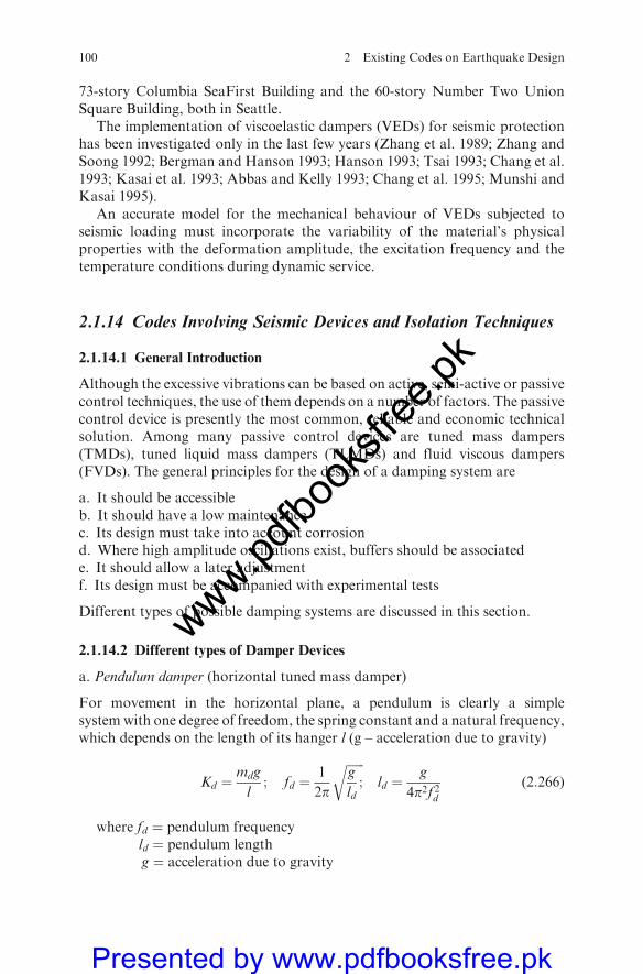
73-story Columbia SeaFirst Building and the 60-story Number Two UnionSquare Building, both in Seattle.
The implementation of viscoelastic dampers (VEDs) for seismic protectionhas been investigated only in the last few years (Zhang et al. 1989; Zhang andSoong 1992; Bergman and Hanson 1993; Hanson 1993; Tsai 1993; Chang et al.1993; Kasai et al. 1993; Abbas and Kelly 1993; Chang et al. 1995; Munshi andKasai 1995).
An accurate model for the mechanical behaviour of VEDs subjected toseismic loading must incorporate the variability of the material’s physicalproperties with the deformation amplitude, the excitation frequency and thetemperature conditions during dynamic service.
2.1.14 Codes Involving Seismic Devices and Isolation Techniques
2.1.14.1 General Introduction
Although the excessive vibrations can be based on active, semi-active or passivecontrol techniques, the use of them depends on a number of factors. The passivecontrol device is presently the most common, reliable and economic technicalsolution. Among many passive control devices are tuned mass dampers(TMDs), tuned liquid mass dampers (TLMDs) and fluid viscous dampers(FVDs). The general principles for the design of a damping system are
a. It should be accessibleb. It should have a low maintenancec. Its design must take into account corrosiond. Where high amplitude oscillations exist, buffers should be associatede. It should allow a later adjustmentf. Its design must be accompanied with experimental tests
Different types of possible damping systems are discussed in this section.
2.1.14.2 Different types of Damper Devices
a. Pendulum damper (horizontal tuned mass damper)
For movement in the horizontal plane, a pendulum is clearly a simplesystemwith one degree of freedom, the spring constant and a natural frequency,which depends on the length of its hanger l (g – acceleration due to gravity)
Kd ¼mdg
l; fd ¼
1
2p
ffiffiffiffiffiffig
ld;
rld ¼
g
4p2f 2d(2:266)
where fd ¼ pendulum frequencyld ¼ pendulum lengthg ¼ acceleration due to gravity
100 2 Existing Codes on Earthquake Design
www.pdfbo
oksfr
ee.pk
Presented by www.pdfbooksfree.pk
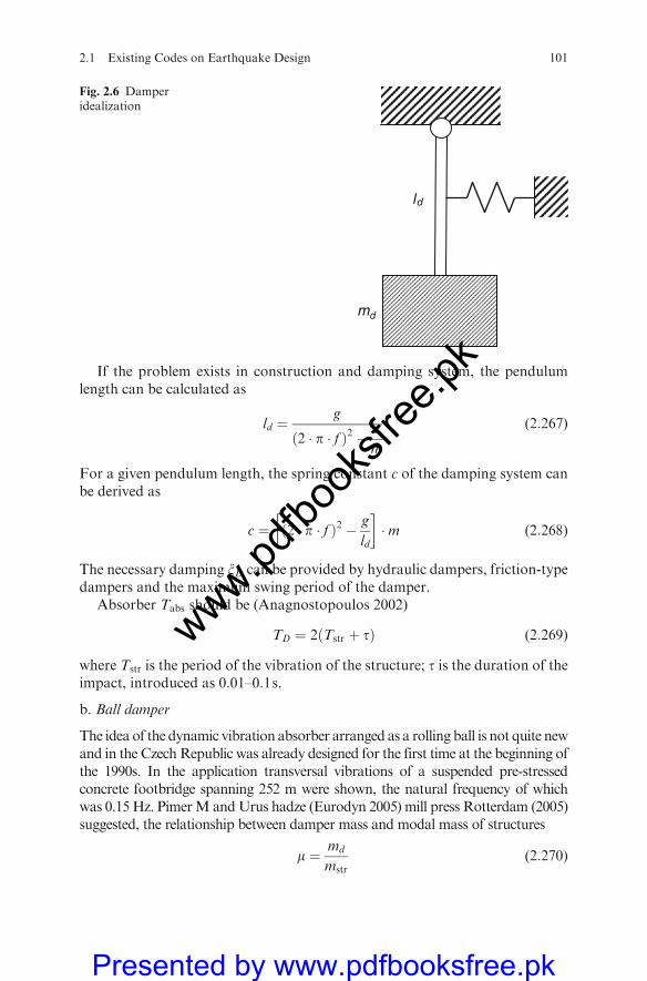
If the problem exists in construction and damping system, the pendulumlength can be calculated as
ld ¼g
ð2 � p � f Þ2 � c
m
(2:267)
For a given pendulum length, the spring constant c of the damping system canbe derived as
c ¼ ð2 � p � f Þ2 � g
ld
� ��m (2:268)
The necessary damping xD can be provided by hydraulic dampers, friction-typedampers and the maximum swing period of the damper.
Absorber Tabs should be (Anagnostopoulos 2002)
TD ¼ 2ðTstr þ tÞ (2:269)
where Tstr is the period of the vibration of the structure; t is the duration of theimpact, introduced as 0.01–0.1s.
b. Ball damper
The idea of the dynamic vibration absorber arranged as a rolling ball is not quite newand in the Czech Republic was already designed for the first time at the beginning ofthe 1990s. In the application transversal vibrations of a suspended pre-stressedconcrete footbridge spanning 252 m were shown, the natural frequency of whichwas 0.15 Hz. PimerM andUrus hadze (Eurodyn 2005) mill press Rotterdam (2005)suggested, the relationship between damper mass and modal mass of structures
m ¼ md
mstr(2:270)
ld
dm
Fig. 2.6 Damperidealization
2.1 Existing Codes on Earthquake Design 101
www.pdfbo
oksfr
ee.pk
Presented by www.pdfbooksfree.pk
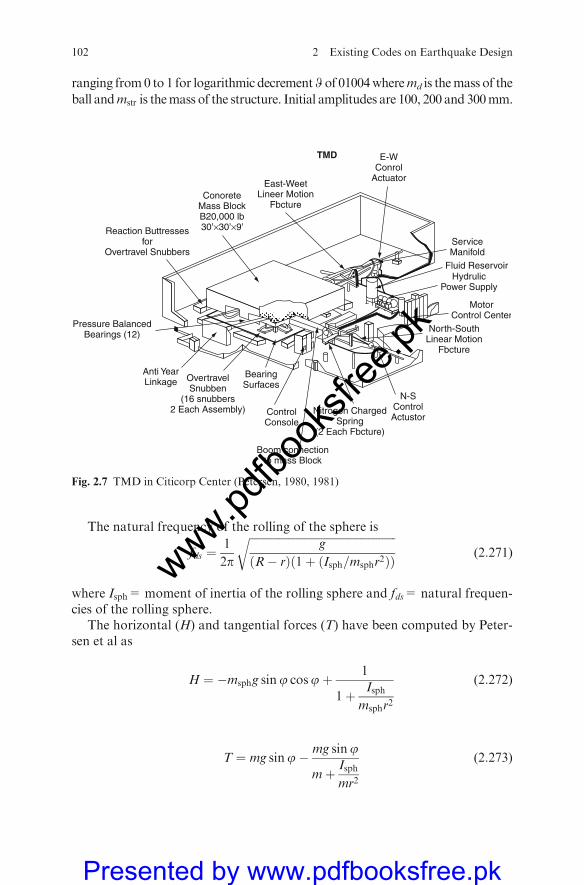
ranging from0 to 1 for logarithmic decrementW of 01004wheremd is themass of the
ball andmstr is themass of the structure. Initial amplitudes are 100, 200 and 300mm.
The natural frequency of the rolling of the sphere is
fds ¼1
2p
ffiffiffiffiffiffiffiffiffiffiffiffiffiffiffiffiffiffiffiffiffiffiffiffiffiffiffiffiffiffiffiffiffiffiffiffiffiffiffiffiffiffiffiffiffiffiffiffiffiffiffiffiffig
ðR� rÞð1þ ðIsph=msphr2ÞÞ
r(2:271)
where Isph= moment of inertia of the rolling sphere and fds= natural frequen-cies of the rolling sphere.
The horizontal (H) and tangential forces (T) have been computed by Peter-sen et al as
H ¼ �msphg sinj cosjþ 1
1þ Isphmsphr2
(2:272)
T ¼ mg sinj� mg sinj
mþ Isphmr2
(2:273)
East-WeetLineer Motion
FbctureConorete
Mass BlockB20,000 lb30’×30’×9’Reaction Buttresses
forOvertravel Snubbers
Pressure BalancedBearings (12)
Anti YearLinkage Overtravel
Snubben(16 snubbers
2 Each Assembly) ControlConsole
Boom connectionto mass Block
Nitrogen ChargedSpring
(2 Each Fbcture)
N-SControlActustor
North-SouthLinear Motion
Fbcture
MotorControl Center
HydrulicPower Supply
Fluid Reservoir
ServiceManifold
BearingSurfaces
E-WConrol
Actuator
TMD
Fig. 2.7 TMD in Citicorp Center (Petersen, 1980, 1981)
102 2 Existing Codes on Earthquake Design
www.pdfbo
oksfr
ee.pk
Presented by www.pdfbooksfree.pk
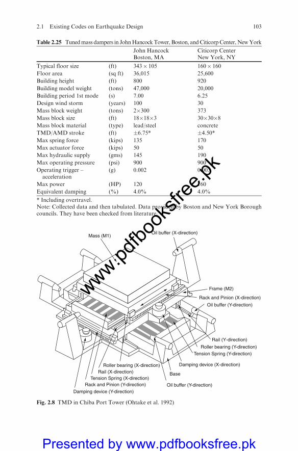
Table 2.25 Tunedmass dampers in JohnHancockTower, Boston, andCiticorpCenter,NewYork
John HancockBoston, MA
Citicorp CenterNew York, NY
Typical floor size (ft) 343� 105 160� 160
Floor area (sq ft) 36,015 25,600
Building height (ft) 800 920
Building model weight (tons) 47,000 20,000
Building period 1st mode (s) 7.00 6.25
Design wind storm (years) 100 30
Mass block weight (tons) 2�300 373
Mass block size (ft) 18�18�3 30�30�8Mass block material (type) lead/steel concrete
TMD/AMD stroke (ft) �6.75* �4.50*Max spring force (kips) 135 170
Max actuator force (kips) 50 50
Max hydraulic supply (gms) 145 190
Max operating pressure (psi) 900 900
Operating trigger –acceleration
(g) 0.002 0.003
Max power (HP) 120 160
Equivalent damping (%) 4.0% 4.0%
* Including overtravel.Note: Collected data and then tabulated. Data provided by Boston and New York Boroughcouncils. They have been checked from literature.
Roller bearing (X-direction)
Oil buffer (Y-direction)
Oil buffer (X-direction)Mass (M1)
Oil buffer (Y-direction)
Damping device (X-direction)
Tension Spring (Y-direction)Roller bearing (Y-direction)
Rail (Y-direction)
BaseRail (X-direction)Tension Spring (X-direction)
Rack and Pinion (Y-direction)
Rack and Pinion (X-direction)
Frame (M2)
Damping device (Y-direction)
Fig. 2.8 TMD in Chiba Port Tower (Ohtake et al. 1992)
2.1 Existing Codes on Earthquake Design 103
www.pdfbo
oksfr
ee.pk
Presented by www.pdfbooksfree.pk
c. Tuned mass damper
Petersen [1995] provides a method design for tuned mass dampers using equation(2.279)
Calculation of damper mass:
md ¼ mh � m (2:274)
Calculation of optimum turning Kopt and of optimum damping ratio xopt:
Kopt ¼ 1=1þ m (2:275)
xopt ¼ffiffiffi3p� m=8 � 1þ mð Þ3 (2:276)
Calculation of the optimum damping frequency, fd :
fd ¼ Kopt � fh (2:277)
Calculation of the spring constant of the damping element, kd :
kd ¼ 2 � p � fdð Þ2� md (2:278)
Calculation of the damping coefficient of the damping element, ddc:
ddc ¼ 2 �md � 2 � p � fdð Þ � xopt (2:279)
d. Viscous dampers
Viscous elastic dampers or dry friction dampers use the action of solids todissipate the oscillatory energy of a structure. It is also possible to use a fluidfor obtaining the same goal.
The immediate device is the one derived from the ‘‘dashpot’’. In such adevice, the dissipation is obtained by the conversion of the mechanical energyinto heat with the help of a piston that deforms and displaces a very viscoussubstance such as silicon. Another family of dampers is based on the flow of afluid in a closed container. The piston not only deforms the viscous substancebut also forces the passage of the fluid through calibrated orifices. As in thepreceding case, the dissipation of the energy results in development of the heat.
The main difference between these two techniques is the following. In the‘‘dashpot’’ damper, the dissipative force is a function of the viscosity of the fluid,while in the other one that force is principally due to the volumic mass of thefluid. This means that the dampers with orifices are more stable against tem-perature variations in comparison with the ‘‘dashpot’’ ones.
Viscous dampers must be placed between two points of the structure withdifferential displacement between them. They can be either on an elementlinking a pier and the deck or on the horizontal wind bracing of the deck.
104 2 Existing Codes on Earthquake Design
www.pdfbo
oksfr
ee.pk
Presented by www.pdfbooksfree.pk
Several recent studies have shown that supplement fluid viscous damping
effectively reduces the seismic responses of asymmetric plan systems. However,
these investigations examined the behaviour of asymmetric plan systems
with linear fluid viscous dampers. Non-linear fluid viscous dampers (velocity
exponent less than one) have the apparent advantage of limiting the peak damper
force at large velocities while still providing sufficient supplemental damping for
linear dampers, the damper force increasing linearly with damper velocity.A recent investigation examined the seismic response of asymmetric systems
with non-linear viscous and viscoelastic dampers. It was found that structural
response is weakly affected by damper non-linearity, and non-linear dampers
achieve essentially the same reduction in response but with much smaller
damper force compared to linear dampers; reductions up to 20%were observed
for edge deformations and plan rotations of short-period systems. Further-
more, it was shown that the earthquake response of the asymmetric systems
with non-linear dampers can be estimated with sufficient degree of accuracy by
analysing the same asymmetric systems with equivalent linear dampers.
A simplified analysis procedure for asymmetric plan systems with non-linear
dampers has also been developed.The investigation by Lin and Chopra examined the effects of damper
non-linearity on edge deformations and damper forces. For asymmetric plan
systems, however, other important response quantities of interest for design
purposes include base shear, base torque and base torque generated by asym-
metric distribution of dampers. Therefore, it is useful to investigate the effects of
damper non-linearity on these responses.
e. Viscous elastic dampers
The use of viscous elastic materials for the control of vibrations goes back to the
1950s. Their application in structural engineering dates back to the 1960s.The viscous elastic materials are principally polymers dissipating the energy
by shear. The characteristics of viscous elastic dampers depend not only on
frequency but also on temperature. The damping coefficient is expressed by
C ¼ Wd
p � O � x2 (2:280)
where Wd ¼ energy dissipation in the structure per cycleO ¼ circular frequency of excitationx ¼ (piston) displacement
To calculate the effect of dampers in the structure a time history dynamic
analysis could be carried out. Viscoelastic damper’s behaviour could be repre-
sented with the following simplified model:
F ¼ F0 þ Kxþ Cva (2:281)
2.1 Existing Codes on Earthquake Design 105
www.pdfbo
oksfr
ee.pk
Presented by www.pdfbooksfree.pk
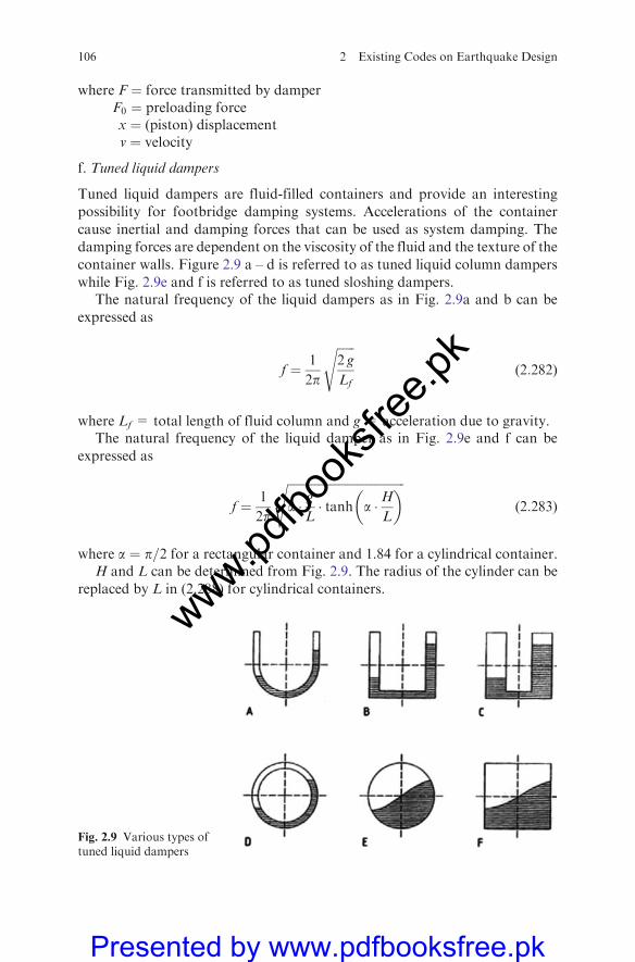
where F ¼ force transmitted by damperF0 ¼ preloading forcex ¼ (piston) displacementv ¼ velocity
f. Tuned liquid dampers
Tuned liquid dampers are fluid-filled containers and provide an interesting
possibility for footbridge damping systems. Accelerations of the container
cause inertial and damping forces that can be used as system damping. The
damping forces are dependent on the viscosity of the fluid and the texture of the
container walls. Figure 2.9 a – d is referred to as tuned liquid column dampers
while Fig. 2.9e and f is referred to as tuned sloshing dampers.The natural frequency of the liquid dampers as in Fig. 2.9a and b can be
expressed as
f ¼ 1
2p
ffiffiffiffiffiffi2 g
Lf
s(2:282)
where Lf = total length of fluid column and g = acceleration due to gravity.The natural frequency of the liquid damper as in Fig. 2.9e and f can be
expressed as
f ¼ 1
2p
ffiffiffiffiffiffiffiffiffiffiffiffiffiffiffiffiffiffiffiffiffiffiffiffiffiffiffiffiffiffiffiffiffiffiffiffiffiffiffia � g
L� tanh a �H
L
� �s(2:283)
where a ¼ p=2 for a rectangular container and 1.84 for a cylindrical container.H and L can be determined from Fig. 2.9. The radius of the cylinder can be
replaced by L in (2.288) for cylindrical containers.
Fig. 2.9 Various types oftuned liquid dampers
106 2 Existing Codes on Earthquake Design
www.pdfbo
oksfr
ee.pk
Presented by www.pdfbooksfree.pk
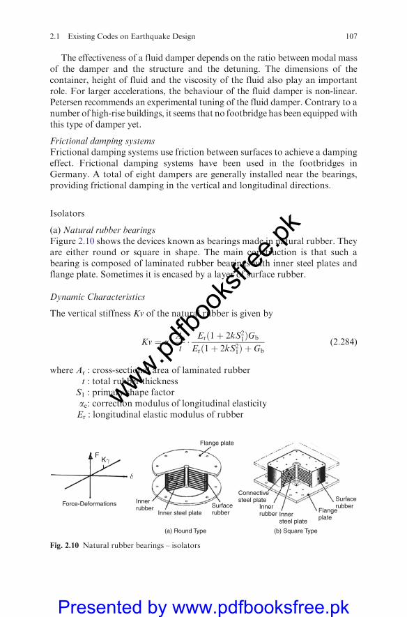
The effectiveness of a fluid damper depends on the ratio between modal massof the damper and the structure and the detuning. The dimensions of thecontainer, height of fluid and the viscosity of the fluid also play an importantrole. For larger accelerations, the behaviour of the fluid damper is non-linear.Petersen recommends an experimental tuning of the fluid damper. Contrary to anumber of high-rise buildings, it seems that no footbridge has been equippedwiththis type of damper yet.
Frictional damping systemsFrictional damping systems use friction between surfaces to achieve a dampingeffect. Frictional damping systems have been used in the footbridges inGermany. A total of eight dampers are generally installed near the bearings,providing frictional damping in the vertical and longitudinal directions.
Isolators
(a) Natural rubber bearingsFigure 2.10 shows the devices known as bearings made in natural rubber. Theyare either round or square in shape. The main construction is that such abearing is composed of laminated rubber bearings with inner steel plates andflange plate. Sometimes it is encased by a layer of surface rubber.
Dynamic Characteristics
The vertical stiffness Kv of the natural rubber is given by
Kv ¼ a � Ar
t� Erð1þ 2kS2
1ÞGb
Erð1þ 2kS21Þ þ Gb
(2:284)
where Ar : cross-sectional area of laminated rubbert : total rubber thickness
S1 : primary shape factorae: correction modulus of longitudinal elasticityEr : longitudinal elastic modulus of rubber
Force-Deformations
FKγ
δ
Innerrubber
Connectivesteel plate
Innerrubber Inner
steel plate
Flangeplate
Surfacerubber
Inner steel plateSurfacerubber
Flange plate
(a) Round Type (b) Square Type
Fig. 2.10 Natural rubber bearings – isolators
2.1 Existing Codes on Earthquake Design 107
www.pdfbo
oksfr
ee.pk
Presented by www.pdfbooksfree.pk
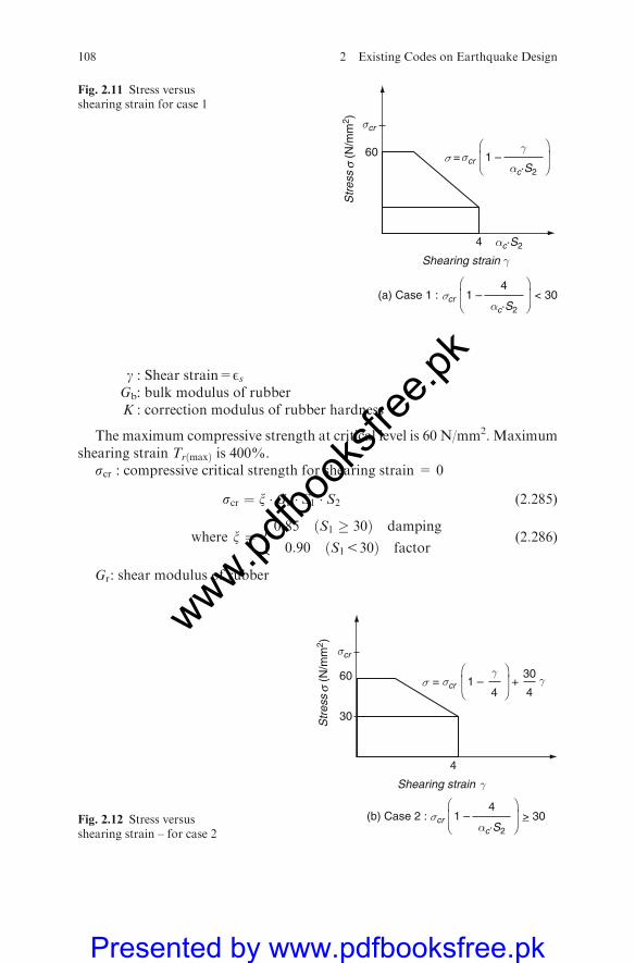
g : Shear strain=EsGb: bulk modulus of rubberK : correction modulus of rubber hardness
The maximum compressive strength at critical level is 60 N/mm2. Maximumshearing strain TrðmaxÞ is 400%.
scr : compressive critical strength for shearing strain = 0
scr ¼ x � Gr � S1 � S2 (2:285)
where x ¼0:85 S1 � 30ð Þ damping
0:90 S1530ð Þ factor
�(2:286)
Gr: shear modulus of rubber
Str
ess
(N
/mm
2 )σ σ
σcr
= σcr
Shearing strain γ
γ60
30
1 – + ⎛⎜⎝
⎞⎟⎠
4
4 4
30
σcr 1 – (b) Case 2 : > 304⎛
⎜⎝
⎞⎟⎠αc·S2
γ
Fig. 2.12 Stress versusshearing strain – for case 2
Str
ess
(N
/mm
2 )σ σ
σcr
= σcr
Shearing strain γ
γ60 1 – ⎛⎜⎝
⎞⎟⎠
4 αc·S 2
αc·S 2
σcr 1 – (a) Case 1 : < 304⎛
⎜⎝
⎞⎟⎠αc·S2
Fig. 2.11 Stress versusshearing strain for case 1
108 2 Existing Codes on Earthquake Design
www.pdfbo
oksfr
ee.pk
Presented by www.pdfbooksfree.pk
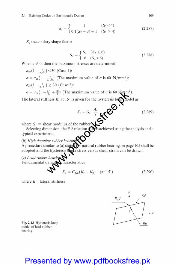
ac ¼1 S254ð Þ
0:1 S2 � 3ð Þ þ 1 S2 � 4ð Þ
�(2:287)
S2 : secondary shape factor
S2 ¼S2 S2 � 6ð Þ6 S246ð Þ
�(2:288)
When g 6¼ 0, then the maximum stresses are determined.
scr 1� 4
ac�S2
�530 Case 1ð Þ:
s ¼ scr 1� g
ac�S2
� The maximum value of s is 60 N=mm2
�:
scr 1� 4
ac�S2
�� 30
Case 2
�:
s ¼ scr 1� g4
�þ 30
4g The maximum value of s is 60N/mm2 �
:
The lateral stiffness Kr at 15 is given for the hysteresis loop model as
Kr ¼ Gr �Ar
t(2:289)
where Gr = shear modulus of the rubber.Selecting dimension, the F-8 relation can be achieved using the analysis and a
typical experiment.
(b) High damping rubber bearingAprocedure similar to (a) stated for natural rubber bearing on page 105 shall be
adopted and the hysteresis shear stress versus shear strain can be drawn.
(c) Lead-rubber bearingFundamental dynamic characteristics
Kd ¼ CKd Kr þ Kp
�at 15ð Þ (2:290)
where Kr : lateral stiffness
F
δ
Kd
Ku
Fγ d
Fig. 2.13 Hysteresis loopmodel of lead-rubberbearing
2.1 Existing Codes on Earthquake Design 109
www.pdfbo
oksfr
ee.pk
Presented by www.pdfbooksfree.pk
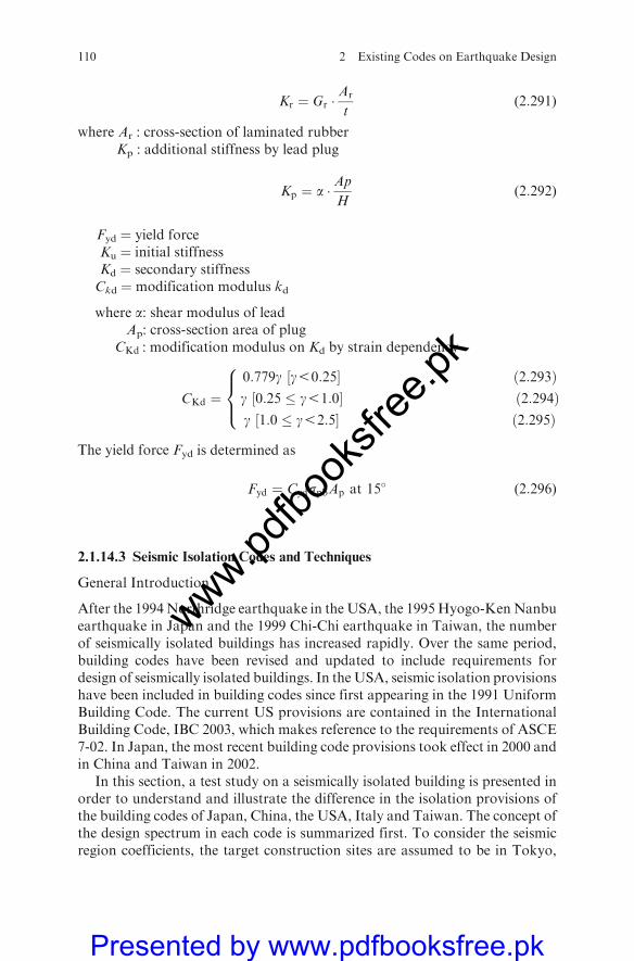
Kr ¼ Gr �Ar
t(2:291)
where Ar : cross-section of laminated rubberKp : additional stiffness by lead plug
Kp ¼ a � ApH
(2:292)
Fyd ¼ yield forceKu ¼ initial stiffnessKd ¼ secondary stiffnessCkd ¼ modification modulus kd
where a: shear modulus of leadAp: cross-section area of plug
CKd : modification modulus on Kd by strain dependency
CKd ¼0:779g g50:25½ ð2:293Þg 0:25 � g51:0½ ð2:294Þg 1:0 � g52:5½ ð2:295Þ
8><>:
The yield force Fyd is determined as
Fyd ¼ CydspbAp at 15 (2:296)
2.1.14.3 Seismic Isolation Codes and Techniques
General Introduction
After the 1994Northridge earthquake in the USA, the 1995Hyogo-KenNanbuearthquake in Japan and the 1999 Chi-Chi earthquake in Taiwan, the numberof seismically isolated buildings has increased rapidly. Over the same period,building codes have been revised and updated to include requirements fordesign of seismically isolated buildings. In theUSA, seismic isolation provisionshave been included in building codes since first appearing in the 1991 UniformBuilding Code. The current US provisions are contained in the InternationalBuilding Code, IBC 2003, which makes reference to the requirements of ASCE7-02. In Japan, the most recent building code provisions took effect in 2000 andin China and Taiwan in 2002.
In this section, a test study on a seismically isolated building is presented inorder to understand and illustrate the difference in the isolation provisions ofthe building codes of Japan, China, the USA, Italy and Taiwan. The concept ofthe design spectrum in each code is summarized first. To consider the seismicregion coefficients, the target construction sites are assumed to be in Tokyo,
110 2 Existing Codes on Earthquake Design
www.pdfbo
oksfr
ee.pk
Presented by www.pdfbooksfree.pk

Beijing, Los Angeles, Potenza and Taipei, respectively. A fixed soil profile isassumed in all cases where the average shear wave velocity within the top 30m isabout 209 m/s.
If the control device needs external energy to modify the vibration propertiesof a structure, a closed-loop control system can be used, which does not affectmany properties of external vibrations. In the case of an open loop controlsystem external vibrations are sensed as soon as they reach the foundation andbefore they are incident on the building. The control is exercised in such a waythat the building does not vibrate in resonance with the severe changes inseismic motion. The usefulness of the open-loop system depends on the properfunctioning of the brain unit which recognizes the information from varioussensors and generates signals to counter the earthquake.
Various devices are being considered for the control mechanism. Themain mechanisms being discussed are (a) variable stiffness mechanism wherestiffness of the structure is varied according to the seismic motion striking thefoundation of the building so that the building does not attain resonancecondition and (b) a mechanism requiring external energy or a mechanismwith additional control power which actively and effectively absorbs the energyincident on the building according to the response and which can restore thedeformation caused in the building due to the action of the seismic force.
Design Spectrum
In general, seismic load is expressed by a 5%damped design spectrum as follows:
S Tð Þ ¼ ISa Tð Þ (2:297)
where
I: occupancy importance factor, which is taken as 1.0 in this studyT: fundamental period of the structure
Sa(T ): the design spectrum on site.
The design spectrum generally consists of two parts, namely, a uniform accel-eration portion in the short-period range and a uniform velocity portion in thelonger period range.
In the Chinese code, spectrum in the constant velocity portion is additionallyincreased to ensure the safety of structures having long natural periods, such ashigh-rise buildings or seismically isolated buildings.
A two-stage design philosophy is introduced in the Japanese, Chineseand Italian codes. The two stages are usually defined as damage limitation(level 1) and life safety (level 2). In this chapter, response analyses in the lifesafety stage will be discussed. In addition, an extremely large earthquake with 2%probability of exceedance in 50 years is defined to check the maximum designdisplacement of the isolation system in the US and Italian codes.
2.1 Existing Codes on Earthquake Design 111
www.pdfbo
oksfr
ee.pk
Presented by www.pdfbooksfree.pk
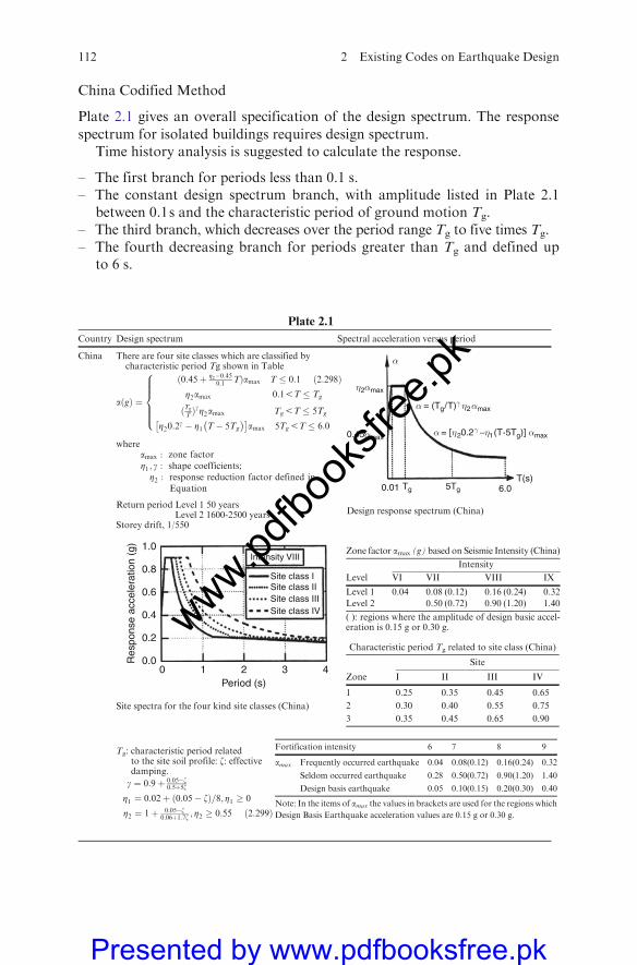
China Codified Method
Plate 2.1 gives an overall specification of the design spectrum. The response
spectrum for isolated buildings requires design spectrum.Time history analysis is suggested to calculate the response.
– The first branch for periods less than 0.1 s.– The constant design spectrum branch, with amplitude listed in Plate 2.1
between 0.1s and the characteristic period of ground motion Tg.– The third branch, which decreases over the period range Tg to five times Tg.– The fourth decreasing branch for periods greater than Tg and defined up
to 6 s.
Plate 2.1
Country Design spectrum Spectral acceleration versus period
China There are four site classes which are classified bycharacteristic period Tg shown in Table
a gð Þ ¼
ð0:45þ Z2�0:450:1 TÞamax T � 0:1 ð2:298Þ
Z2amax 0:15T � Tg
ðTg
T ÞgZ2amax Tg5T � 5Tg
Z20:2g � Z1 T� 5Tg
� amax 5Tg5T � 6:0
8>>>><>>>>:
whereamax : zone factorZ1 ; g : shape coefficients;Z2 : response reduction factor defined in
Equation
Return period Level 1 50 yearsLevel 2 1600-2500 years
Storey drift, 1/550
1.0Intensity VIII
Site class ISite class IISite class IIISite class IV
0.8
0.6
0.4
0.2
Res
pons
e ac
cele
ratio
n (g
)
0.00 1 2 3 4
Period (s)
Site spectra for the four kind site classes (China)
Tg: characteristic period relatedto the site soil profile: z: effectivedamping.
g ¼ 0:9þ 0:05�z0:5þ5z
Z1 ¼ 0:02þ 0:05� zð Þ=8; Z1 � 0
Z2 ¼ 1þ 0:05�z0:06þ1:7z ; Z2 � 0:55 ð2:299Þ
0.45α max
0.01 6.0T(s)
Tg 5Tg
η 2α max
α
α = (Tg / T)γ η 2 α max
α = [η 20.2 γ −η1 (T.5Tg)] α max
Design response spectrum (China)
Zone factor amax (g) based on Seismie Intensity (China)
Intensity
Level VI VII VIII IX
Level 1 0.04 0.08 (0.12) 0.16 (0.24) 0.32
Level 2 0.50 (0.72) 0.90 (1.20) 1.40
( ): regions where the amplitude of design basic accel-eration is 0.15 g or 0.30 g.
Characteristic period Tg related to site class (China)
Site
Zone I II III IV
1 0.25 0.35 0.45 0.65
2 0.30 0.40 0.55 0.75
3 0.35 0.45 0.65 0.90
Fortification intensity 6 7 8 9
amax Frequently occurred earthquake 0.04 0.08(0.12) 0.16(0.24) 0.32
Seldom occurred earthquake 0.28 0.50(0.72) 0.90(1.20) 1.40
Design basis earthquake 0.05 0.10(0.15) 0.20(0.30) 0.40
Note: In the items of amax the values in brackets are used for the regions which
Design Basis Earthquake acceleration values are 0.15 g or 0.30 g.
112 2 Existing Codes on Earthquake Design
www.pdfbo
oksfr
ee.pk
Presented by www.pdfbooksfree.pk
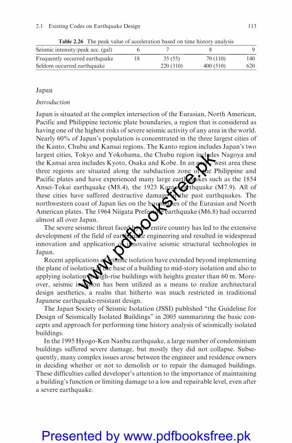
Japan
Introduction
Japan is situated at the complex intersection of the Eurasian, North American,
Pacific and Philippine tectonic plate boundaries, a region that is considered as
having one of the highest risks of severe seismic activity of any area in the world.
Nearly 60% of Japan’s population is concentrated in the three largest cities of
the Kanto, Chubu and Kansai regions. The Kanto region includes Japan’s two
largest cities, Tokyo and Yokohama, the Chubu region includes Nagoya and
the Kansai area includes Kyoto, Osaka and Kobe. In an east – west area these
three regions are situated along the subduction zone of the Philippine and
Pacific plates and have experienced many large earthquakes such as the 1854
Ansei-Tokai earthquake (M8.4), the 1923 Kanto earthquake (M7.9). All of
these cities have suffered destructive damage in the past earthquakes. The
northwestern coast of Japan lies on the boundaries of the Eurasian and North
American plates. The 1964 Niigata Prefecture earthquake (M6.8) had occurred
almost all over Japan.The severe seismic threat faced by the entire country has led to the extensive
development of the field of earthquake engineering and resulted in widespread
innovation and application of innovative seismic structural technologies in
Japan.Recent applications of seismic isolation have extended beyond implementing
the plane of isolation at the base of a building to mid-story isolation and also to
applying isolation to high-rise buildings with heights greater than 60 m. More-
over, seismic isolation has been utilized as a means to realize architectural
design aesthetics, a realm that hitherto was much restricted in traditional
Japanese earthquake-resistant design.The Japan Society of Seismic Isolation (JSSI) published ‘‘the Guideline for
Design of Seismically Isolated Buildings’’ in 2005 summarizing the basic con-
cepts and approach for performing time history analysis of seismically isolated
buildings.In the 1995Hyogo-KenNanbu earthquake, a large number of condominium
buildings suffered severe damage, but mostly they did not collapse. Subse-
quently, many complex issues arose between the engineer and residence owners
in deciding whether or not to demolish or to repair the damaged buildings.
These difficulties called developer’s attention to the importance of maintaining
a building’s function or limiting damage to a low and repairable level, even after
a severe earthquake.
Table 2.26 The peak value of acceleration based on time history analysis
Seismic intensity/peak acc. (gal) 6 7 8 9
Frequently occurred earthquake 18 35 (55) 70 (110) 140
Seldom occurred earthquake 220 (310) 400 (510) 620
2.1 Existing Codes on Earthquake Design 113
www.pdfbo
oksfr
ee.pk
Presented by www.pdfbooksfree.pk
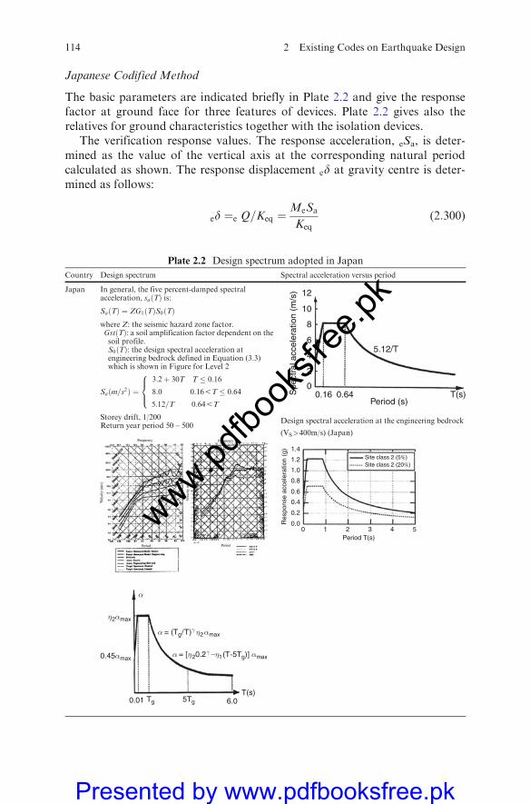
Japanese Codified Method
The basic parameters are indicated briefly in Plate 2.2 and give the responsefactor at ground face for three features of devices. Plate 2.2 gives also therelatives for ground characteristics together with the isolation devices.
The verification response values. The response acceleration, eSa, is deter-mined as the value of the vertical axis at the corresponding natural periodcalculated as shown. The response displacement ed at gravity centre is deter-mined as follows:
ed ¼e Q=Keq ¼MeSa
Keq(2:300)
Plate 2.2 Design spectrum adopted in Japan
Country Design spectrum Spectral acceleration versus period
Japan In general, the five percent-damped spectralacceleration, saðTÞ is:SaðTÞ ¼ ZG1ðTÞS0ðTÞwhere Z: the seismic hazard zone factor.GstðTÞ: a soil amplification factor dependent on thesoil profile.S0ðTÞ: the design spectral acceleration atengineering bedrock defined in Equation (3.3)which is shown in Figure for Level 2
Saðm=s2Þ ¼3:2þ 30T T � 0:16
8:0 0:165T � 0:64
5:12=T 0:645T
8><>:
Storey drift, 1/200Return year period 50 – 500
0.45α max
0.01 6.0T(s)
Tg 5Tg
η 2α max
α
α = (Tg / T)γ η 2 α max
α = [η 20.2 γ −η1 (T.5Tg)] α max
12
10
8
6
4
2
00.16 0.64 T(s)
Period (s)
5.12/T
Spe
ctra
l acc
eler
atio
n (m
/s)
Design spectral acceleration at the engineering bedrock
(VS>400m/s) (Japan)
1.4Site class 2 (5%)Site class 2 (20%)
1.2
1.0
0.8
0.6
0.4
0.2
0.0Res
pons
e ac
cele
ratio
n (g
)
0 1 2Period T(s)
3 4 5
114 2 Existing Codes on Earthquake Design
www.pdfbo
oksfr
ee.pk
Presented by www.pdfbooksfree.pk
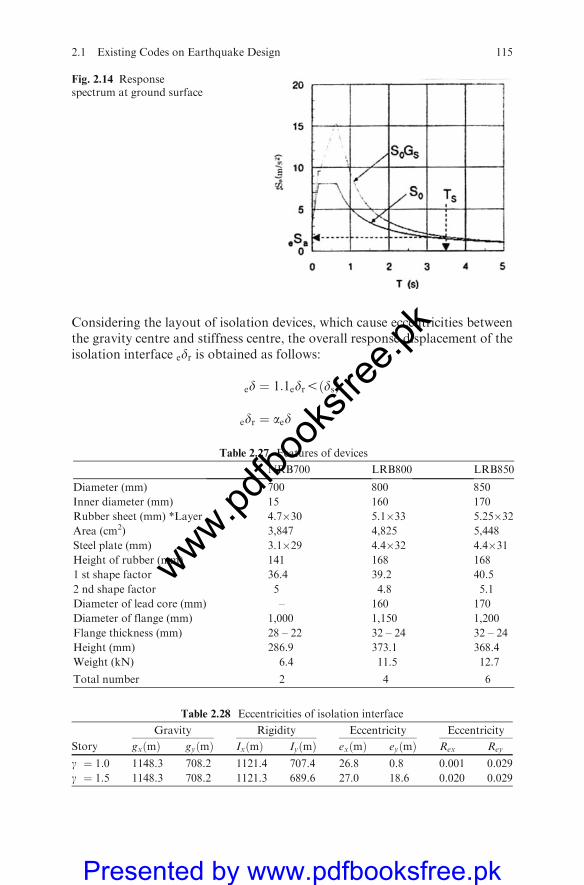
Considering the layout of isolation devices, which cause eccentricities betweenthe gravity centre and stiffness centre, the overall response displacement of theisolation interface edr is obtained as follows:
ed ¼ 1:1edr5ðdsÞ
edr ¼ aed
Fig. 2.14 Responsespectrum at ground surface
Table 2.27 Features of devices
NRB700 LRB800 LRB850
Diameter (mm) 700 800 850
Inner diameter (mm) 15 160 170
Rubber sheet (mm) *Layer 4.7�30 5.1�33 5.25�32Area (cm2) 3,847 4,825 5,448
Steel plate (mm) 3.1�29 4.4�32 4.4�31Height of rubber (mm) 141 168 168
1 st shape factor 36.4 39.2 40.5
2 nd shape factor 5 4.8 5.1
Diameter of lead core (mm) – 160 170
Diameter of flange (mm) 1,000 1,150 1,200
Flange thickness (mm) 28 – 22 32 – 24 32 – 24
Height (mm) 286.9 373.1 368.4
Weight (kN) 6.4 11.5 12.7
Total number 2 4 6
Table 2.28 Eccentricities of isolation interface
Gravity Rigidity Eccentricity Eccentricity
Story gx mð Þ gy mð Þ Ix mð Þ Iy mð Þ ex mð Þ ey mð Þ Rex Rey
g ¼ 1:0 1148.3 708.2 1121.4 707.4 26.8 0.8 0.001 0.029
g ¼ 1:5 1148.3 708.2 1121.3 689.6 27.0 18.6 0.020 0.029
2.1 Existing Codes on Earthquake Design 115
www.pdfbo
oksfr
ee.pk
Presented by www.pdfbooksfree.pk
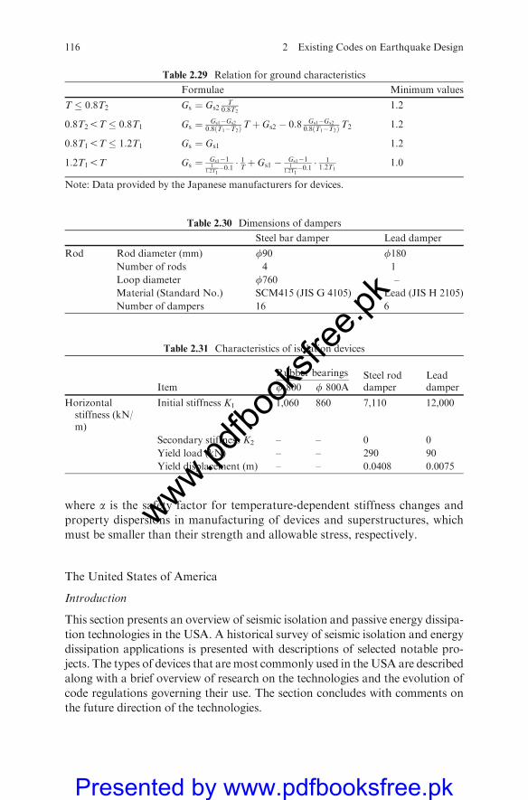
where a is the safety factor for temperature-dependent stiffness changes and
property dispersions in manufacturing of devices and superstructures, which
must be smaller than their strength and allowable stress, respectively.
The United States of America
Introduction
This section presents an overview of seismic isolation and passive energy dissipa-
tion technologies in the USA. A historical survey of seismic isolation and energy
dissipation applications is presented with descriptions of selected notable pro-
jects. The types of devices that are most commonly used in theUSA are described
along with a brief overview of research on the technologies and the evolution of
code regulations governing their use. The section concludes with comments on
the future direction of the technologies.
Table 2.29 Relation for ground characteristics
Formulae Minimum values
T � 0:8T2 Gs ¼ Gs2T
0:8T21.2
0:8T25T � 0:8T1 Gs ¼ Gs1�Gs2
0:8 T1�T2ð ÞTþ Gs2 � 0:8 Gs1�Gs2
0:8 T1�T2ð ÞT2 1.2
0:8T15T � 1:2T1 Gs ¼ Gs1 1.2
1:2T15T Gs ¼ Gs1�11
1:2T1�0:1 �
1Tþ Gs1 � Gs1�1
11:2T1�0:1 �
11:2T1
1.0
Note: Data provided by the Japanese manufacturers for devices.
Table 2.30 Dimensions of dampers
Steel bar damper Lead damper
Rod Rod diameter (mm) f90 f180Number of rods 4 1
Loop diameter f760 –
Material (Standard No.) SCM415 (JIS G 4105) Lead (JIS H 2105)
Number of dampers 16 6
Table 2.31 Characteristics of isolation devices
Item
Rubber bearings Steel roddamper
Leaddamperf 800 f 800A
Horizontalstiffness (kN/m)
Initial stiffness K1 1,060 860 7,110 12,000
Secondary stiffness K2 – – 0 0
Yield load (kN) – – 290 90
Yield displacement (m) – – 0.0408 0.0075
116 2 Existing Codes on Earthquake Design
www.pdfbo
oksfr
ee.pk
Presented by www.pdfbooksfree.pk
Overview of Seismic Isolation Applications in the USA
Construction of the first seismically isolated building in theUSAwas completedin 1985 and by mid-2005 there were approximately 80 seismically isolatedbuildings in the USA. Some of the most significant early projects are discussedbelow, along with examples of several more recent projects.
Buildings
The first building in the USA to be seismically isolated, the Foothill Com-munities Law and Justice Center in Rancho, California, was completed in1985, a four-storey plus basement building. The realization of the project wasthe culmination of the efforts of numerous parties. The use of high-dampingrubber bearings was the first application in the world of this type of isolationsystem.
The US Court of Appeals building, in San Francisco, is another example ofa large historic building retrofit of numerous other monumental buildingstructures, including City Hall in Oakland and State Capitols in South Carolinaand Utah.
Seismic isolation has been used throughout the US buildings up and downthe country; many reports exist on the testing facilities of passive energydissipation systems. However, code provisions for seismic isolation and passiveenergy systems are briefly dealt with below.
Current Status and Future Development
Seismic isolation. Given the 20-year application history of seismic isolation inthe USA, the approximately 80 projects completed is a modest total. Whilemany notable projects, particularly the retrofit of a number of landmarkhistoric buildings, have been undertaken, fewer projects of this type areexpected in the future. Seismic isolation has not moved into the mainstreamas a widely accepted and used seismic-resistant technology.
Somewhat unfairly, seismic isolation has suffered under the conventionalwisdom that it is an expensive technology. Many of the most prominentearly isolation projects were large and costly retrofits of historic buildings,projects that would have been expensive regardless of whether or not isolationwas used. Nonetheless, the general belief has evolved that seismic isolationis expensive and that it is not economically feasible to consider for typicalbuildings.
Codified Method
According to IBC 2003, the general design response spectrum curve withvarious equations are indicated in Plate 2.3.
Apart from these parameters, the values of the site coefficient Fa as afunction of the site class and mapped spectra response acceleration at shortperiod (S) would be needed and they are given below:
2.1 Existing Codes on Earthquake Design 117
www.pdfbo
oksfr
ee.pk
Presented by www.pdfbooksfree.pk

Values of site coefficient Fa as a function of site class and mapped spectral
response are given in tables provided by the code.Based on ISO, the following information is required if one goes on using the code:
Acceleration at short period (Ss)a
Mapped spectral accelerations at short periods
Site ClassA reference is made to the code
Plate 2.3 Design spectrum and Data (U.S.A)Country Design spectrum Spectral acceleration versus period
USA According to the IBC 2003, the general designresponse spectrum curve is as shown in Figureand is defined by Equation
Sa ¼0:6 SDS
T0þ 0:4SDS
SDSSD1
T
8<:
T � T0
T0 � T � TS
TS5T
where:SDS ;SD1 : the design spectral responseacceleration at short periods and one secondperiod, respectively, as determined by Equation(3.8).T0 ¼ 0:2SD1=SDS ;TS ¼ SD1=SDS
SDS ¼ 23SMS ¼ 2
3FaSS
SD1 ¼ 23SM1 ¼ 2
3FvS1
SS � 1:55 g;S1 ¼ 0:623 gWhere:Fa;Fv: site coefficients defined in Tablesand, respectively. Ss ;S1: the mapped spectralaccelerations for short periods and one secondperiod.
Design response spectrum, IBC 2003 (USA)
Site spectra at the four kinds of site classes (USA)
Table Values of the site coefficient Fa as a functions of the class
andmapped spectral response acceleration at short period (Ss)a
Mapped spectral accelerations at short periodsSite Class Ss � 0.25 Ss = 0.50 Ss = 0.75 Ss = 1.00 Ss � 1.25
A 0.8 0.8 0.8 0.8 0.8B 1.0 1.0 1.0 1.0 1.0C 1.2 1.2 1.1 1.0 1.0D 1.6 1.4 1.2 1.1 1.0E 2.5 1.7 1.2 0.9 0.9F Note b Note b Note b Note b Note b
a Use straight line interpolation for intermediate values ofmapped spectral acceleration at short periodb. Site specific geotechnical investigation and dynamic siteresponse analyses shall be performed.
Table Values of site coefficient Fa as a function of site class andmapped
spectral response acceleration at short period (St)a
Mapped spectral accelerations at one second periodSite Class St � 0.1 St ¼ 0.2 St ¼ 0.3 St ¼ 0.4 St � 0.5
A 0.8 0.8 0.8 0.8 0.8B 1.0 1.0 1.0 1.0 1.0C 1.74 1.6 1.5 1.4 1.3D 2.4 2.0 1.8 1.6 1.5E 3.5 3.2 2.8 2.4 2.4F Note b Note b Note b Note b Note b
118 2 Existing Codes on Earthquake Design
www.pdfbo
oksfr
ee.pk
Presented by www.pdfbooksfree.pk
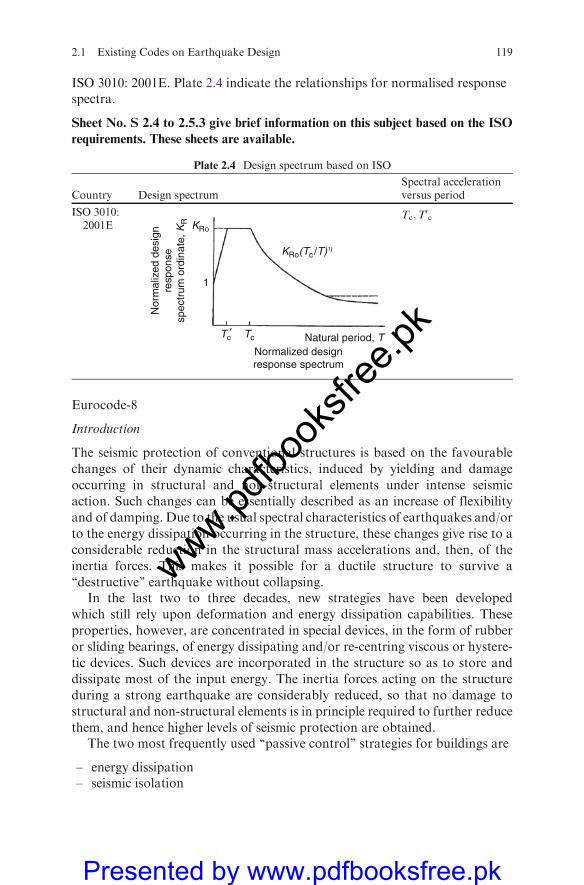
ISO 3010: 2001E. Plate 2.4 indicate the relationships for normalised responsespectra.
Sheet No. S 2.4 to 2.5.3 give brief information on this subject based on the ISO
requirements. These sheets are available.
Eurocode-8
Introduction
The seismic protection of conventional structures is based on the favourable
changes of their dynamic characteristics, induced by yielding and damage
occurring in structural and non-structural elements under intense seismicaction. Such changes can be essentially described as an increase of flexibility
and of damping. Due to the usual spectral characteristics of earthquakes and/or
to the energy dissipation occurring in the structure, these changes give rise to aconsiderable reduction in the structural mass accelerations and, then, of the
inertia forces. This makes it possible for a ductile structure to survive a‘‘destructive’’ earthquake without collapsing.
In the last two to three decades, new strategies have been developed
which still rely upon deformation and energy dissipation capabilities. Theseproperties, however, are concentrated in special devices, in the form of rubber
or sliding bearings, of energy dissipating and/or re-centring viscous or hystere-
tic devices. Such devices are incorporated in the structure so as to store anddissipate most of the input energy. The inertia forces acting on the structure
during a strong earthquake are considerably reduced, so that no damage tostructural and non-structural elements is in principle required to further reduce
them, and hence higher levels of seismic protection are obtained.The two most frequently used ‘‘passive control’’ strategies for buildings are
– energy dissipation– seismic isolation
Plate 2.4 Design spectrum based on ISO
Country Design spectrumSpectral accelerationversus period
ISO 3010:2001E KRo
1
Tc Tc Natural period, TNormalized designresponse spectrum
Nor
mal
ized
des
ign
resp
onse
spec
trum
ord
inat
e, K
R
′
KRo(Tc /T) η
Tc;T0c
2.1 Existing Codes on Earthquake Design 119
www.pdfbo
oksfr
ee.pk
Presented by www.pdfbooksfree.pk
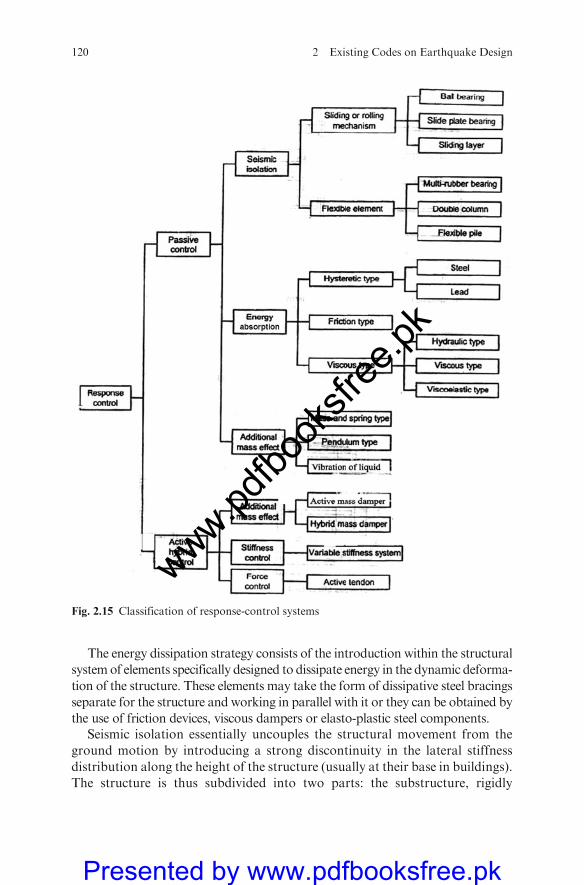
The energy dissipation strategy consists of the introduction within the structural
systemof elements specifically designed to dissipate energy in the dynamic deforma-
tion of the structure. These elements may take the form of dissipative steel bracings
separate for the structure and working in parallel with it or they can be obtained by
the use of friction devices, viscous dampers or elasto-plastic steel components.Seismic isolation essentially uncouples the structural movement from the
ground motion by introducing a strong discontinuity in the lateral stiffness
distribution along the height of the structure (usually at their base in buildings).
The structure is thus subdivided into two parts: the substructure, rigidly
Fig. 2.15 Classification of response-control systems
120 2 Existing Codes on Earthquake Design
www.pdfbo
oksfr
ee.pk
Presented by www.pdfbooksfree.pk
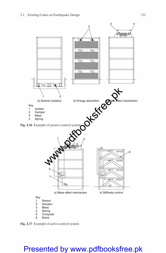
a) Seismic isolation
Key1 Isolator2 Damper3 Mass4 Spring
b) Energy absorbtion c) Mass effect mechanism
2
21
3 4
Fig. 2.16 Example of passive control system
Key1 Sensor2 Actuator3 Mass4 Spring5 Computer6 Brace
a) Mass effect mechanism b) Stiffness control
OFF/ON
ON/OFF
ON/OFF
OFF/ON
1
5
1
4
6
32
Fig. 2.17 Example of active control system
2.1 Existing Codes on Earthquake Design 121
www.pdfbo
oksfr
ee.pk
Presented by www.pdfbooksfree.pk
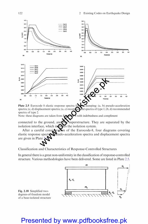
connected to the ground, and the superstructure. They are separated by theisolation interface, which includes the isolation system.
After a careful consideration of the Eurocode-8, four diagrams coveringelastic response spectra, pseudo-acceleration spectra and displacement spectraare given in Plate 2.5
Classification and Characteristics of Response-Controlled Structures
In general there is a great non-uniformity in the classification of response-controlledstructure. Various methodologies have been delivered. Some are listed in Plate 2.5.
Plate 2.5 Eurocode 8 elastic response spectra for 5% damping: (a, b) pseudo-accelerationspectra; (c, d) displacement spectra; (a, c) recommended spectra of type 1; (b, d) recommendedspectra of type 2.Note: these diagrams are taken from Eurocode 8 with indebtedness and compliment
Fig. 2.18 Simplified two-degrees-of-freedom modelof a base-isolated structure
122 2 Existing Codes on Earthquake Design
www.pdfbo
oksfr
ee.pk
Presented by www.pdfbooksfree.pk
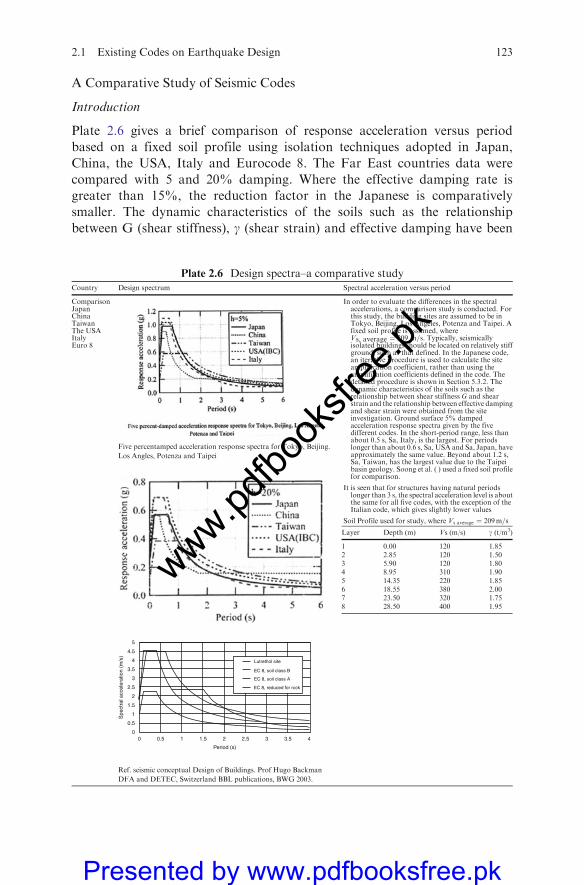
A Comparative Study of Seismic Codes
Introduction
Plate 2.6 gives a brief comparison of response acceleration versus period
based on a fixed soil profile using isolation techniques adopted in Japan,
China, the USA, Italy and Eurocode 8. The Far East countries data were
compared with 5 and 20% damping. Where the effective damping rate is
greater than 15%, the reduction factor in the Japanese is comparatively
smaller. The dynamic characteristics of the soils such as the relationship
between G (shear stiffness), g (shear strain) and effective damping have been
Plate 2.6 Design spectra–a comparative studyCountry Design spectrum Spectral acceleration versus period
ComparisonJapanChinaTaiwanThe USAItalyEuro 8
Five percentamped acceleration response spectra for Tokyo, Beijing.
Los Angles, Potenza and Taipei
00 0.5 1 1.5 2
Period (s)
Spe
ctra
l acc
eler
atio
n (m
/s)
2.5 3
Lutrethol site
EC 8, soil class B
EC 8, soil class A
EC 8, reduced for rock
3.5 4
0.5
1
1.5
2
2.5
3
3.5
4
4.5
5
Ref. seismic conceptual Design of Buildings. Prof Hugo Backman
DFA and DETEC, Switzerland BBL publications, BWG 2003.
In order to evaluate the differences in the spectralaccelerations, a comparison study is conducted. Forthis study, the building sites are assumed to be inTokyo, Beijing, Los Angeles, Potenza and Taipei. Afixed soil profile is assumed, whereVs, average ¼ 209 m=s. Typically, seismicallyisolated buildings should be located on relatively stiffground, such as that defined. In the Japanese code,an iterative procedure is used to calculate the siteamplification coefficient, rather than using theamplification coefficients defined in the code. Thedetailed procedure is shown in Section 5.3.2. Thedynamic characteristics of the soils such as therelationship between shear stiffness G and shearstrain and the relationship between effective dampingand shear strain were obtained from the siteinvestigation. Ground surface 5% dampedacceleration response spectra given by the fivedifferent codes. In the short-period range, less thanabout 0.5 s, Sa, Italy, is the largest. For periodslonger than about 0.6 s, Sa, USA and Sa, Japan, haveapproximately the same value. Beyond about 1.2 s,Sa, Taiwan, has the largest value due to the Taipeibasin geology. Soong et al. ( ) used a fixed soil profilefor comparison.
It is seen that for structures having natural periodslonger than 3 s, the spectral acceleration level is aboutthe same for all five codes, with the exception of theItalian code, which gives slightly lower values
Soil Profile used for study, where Vs average ¼ 209m=s
Layer Depth (m) Vs (m/s) g (t/m3)
1 0.00 120 1.852 2.85 120 1.503 5.90 120 1.804 8.95 310 1.905 14.35 220 1.856 18.55 380 2.007 23.50 320 1.758 28.50 400 1.95
2.1 Existing Codes on Earthquake Design 123
www.pdfbo
oksfr
ee.pk
Presented by www.pdfbooksfree.pk
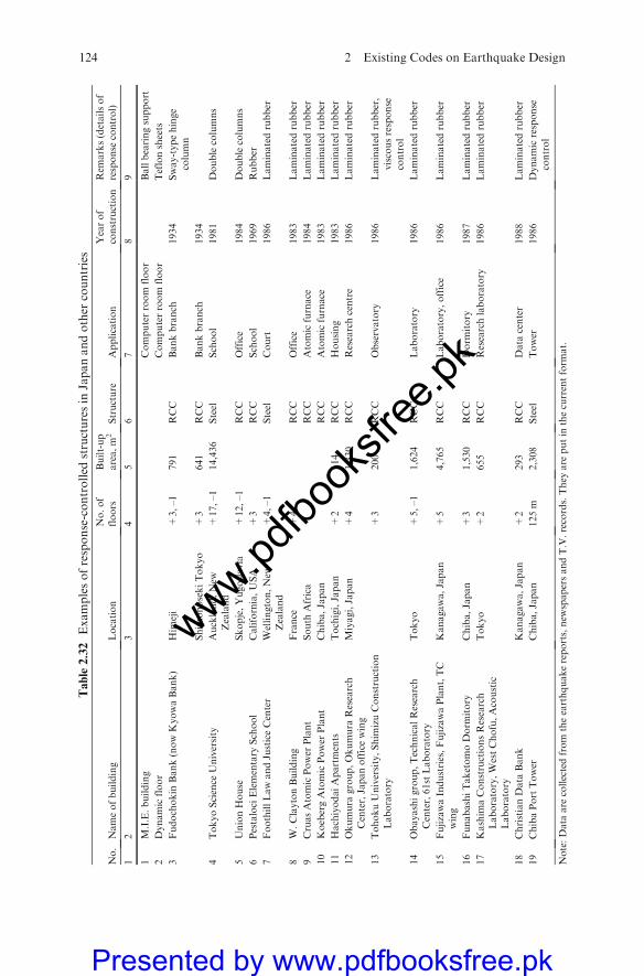
Table2.32
Examplesofresponse-controlled
structuresin
Japanandother
countries
No.
Nameofbuilding
Location
No.of
floors
Built-up
area,m
2Structure
Application
Yearof
construction
Rem
arks(detailsof
response
control)
12
34
56
78
9
1M.I.E.building
Computerroom
floor
Ballbearingsupport
2Dynamicfloor
Computerroom
floor
Teflonsheets
3Fudochokin
Bank(nowKyowaBank)
Him
eji
+3,–1
791
RCC
Bankbranch
1934
Sway-typehinge
column
Shim
onosekiTokyo
+3
641
RCC
Bankbranch
1934
4TokyoScience
University
Auckland,New
Zealand
+17,–1
14,436
Steel
School
1981
Doublecolumns
5UnionHouse
Skopje,Yugoslavia
+12,–1
RCC
Office
1984
Doublecolumns
6PestalociElementary
School
California,USA
+3
RCC
School
1969
Rubber
7FoothillLawandJusticeCenter
Wellington,New
Zealand
+4,–1
Steel
Court
1986
Laminatedrubber
8W.ClaytonBuilding
France
+4
RCC
Office
1983
Laminatedrubber
9CruasAtomicPower
Plant
South
Africa
RCC
Atomicfurnace
1984
Laminatedrubber
10
KoebergAtomicPower
Plant
Chiba,Japan
RCC
Atomicfurnace
1983
Laminatedrubber
11
HachiyodaiApartments
Tochigi,Japan
+2
114
RCC
Housing
1983
Laminatedrubber
12
Okumura
group,Okumura
Research
Center,Japanofficewing
Miyagi,Japan
+4
1,330
RCC
Researchcentre
1986
Laminatedrubber
13
TohokuUniversity,Shim
izuConstruction
Laboratory
+3
200
RCC
Observatory
1986
Laminatedrubber,
viscousresponse
control
14
Obayashigroup,TechnicalResearch
Center,61stLaboratory
Tokyo
+5,–1
1,624
RCC
Laboratory
1986
Laminatedrubber
15
FujizawaIndustries,FujizawaPlant,TC
wing
Kanagawa,Japan
+5
4,765
RCC
Laboratory,office
1986
Laminatedrubber
16
FunabashiTaketomoDorm
itory
Chiba,Japan
+3
1,530
RCC
Dorm
itory
1987
Laminatedrubber
17
Kashim
aConstructionsResearch
Laboratory,WestChofu,Acoustic
Laboratory
Tokyo
+2
655
RCC
Researchlaboratory
1986
Laminatedrubber
18
ChristianData
Bank
Kanagawa,Japan
+2
293
RCC
Data
center
1988
Laminatedrubber
19
ChibaPortTower
Chiba,Japan
125m
2,308
Steel
Tower
1986
Dynamicresponse
control
Note:Data
are
collectedfrom
theearthquakereports,new
spapersandT.V.records.They
are
putin
thecurrentform
at.
124 2 Existing Codes on Earthquake Design
www.pdfbo
oksfr
ee.pk
Presented by www.pdfbooksfree.pk
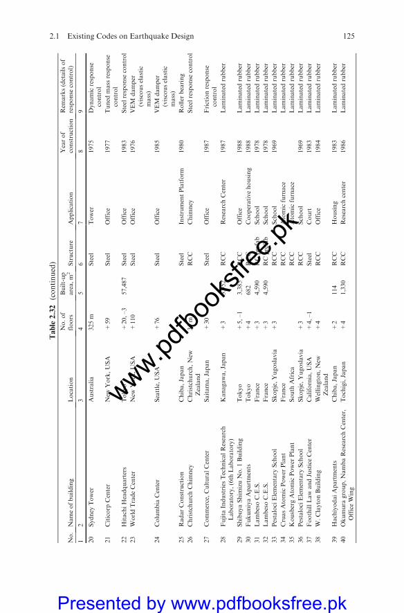
Table2.32
(continued)
No.
Nameofbuilding
Location
No.of
floors
Built-up
area,m
2Structure
Application
Yearof
construction
Rem
arks(detailsof
response
control)
12
34
56
78
9
20
Sydney
Tower
Australia
325m
Steel
Tower
1975
Dynamicresponse
control
21
Citicorp
Center
New
York,USA
+59
Steel
Office
1977
Tuned
mass
response
control
22
HitachiHeadquarters
Tokyo
+20,–3
57,487
Steel
Office
1983
Steelresponse
control
23
WorldTradeCenter
New
York,USA
+110
Steel
Office
1976
VEM
damper
(viscouselastic
mass)
24
Columbia
Center
Seattle,USA
+76
Steel
Office
1985
VEM
damper
(viscouselastic
mass)
25
RadarConstruction
Chiba,Japan
Steel
InstrumentPlatform
1980
Roller
bearing
26
ChristchurchChim
ney
Christchurch,New
Zealand
35m
RCC
Chim
ney
Steelresponse
control
27
Commerce,CulturalCenter
Saitama,Japan
+30
Steel
Office
1987
Frictionresponse
control
28
Fujita
Industries
TechnicalResearch
Laboratory,(6th
Laboratory)
Kanagawa,Japan
+3
3,952
RCC
ResearchCenter
1987
Laminatedrubber
29
ShibuyaShim
izuNo.1Building
Tokyo
+5,–1
3,385
RCC
Office
1988
Laminatedrubber
30
FukumiyaApartments
Tokyo
+4
682
RCC
Cooperativehousing
1988
Laminatedrubber
31
LambesoC.E.S.
France
+3
4,590
RCprefab
School
1978
Laminatedrubber
32
LambesoC.E.S.
France
+3
4,590
RCprefab
School
1978
Laminatedrubber
33
PestalociElementary
School
Skopje,Yugoslavia
+3
RCC
School
1969
Laminatedrubber
34
CruasAtomicPower
Plant
France
RCC
Atomicfurnace
Laminatedrubber
35
KousbergAtomicPower
Plant
South
Africa
RCC
Atomicfurnace
Laminatedrubber
36
PestalociElementary
School
Skopje,Yugoslavia
+3
RCC
School
1969
Laminatedrubber
37
FoothillLawandJusticeCenter
California,USA
+4,–1
Steel
Court
1983
Laminatedrubber
38
W.ClaytonBuilding
Wellington,New
Zealand
+4
RCC
Office
1984
Laminatedrubber
39
HachiyodaiApartments
Chiba,Japan
+2
114
RCC
Housing
1983
Laminatedrubber
40
Okumura
group,NambaResearchCenter,
OfficeWing
Tochigi,Japan
+4
1,330
RCC
Researchcenter
1986
Laminatedrubber
2.1 Existing Codes on Earthquake Design 125
www.pdfbo
oksfr
ee.pk
Presented by www.pdfbooksfree.pk

Table2.32
(continued)
No.
Nameofbuilding
Location
No.of
floors
Built-up
area,m
2Structure
Application
Yearof
construction
Rem
arks(detailsof
response
control)
12
34
56
78
9
41
Obayashigroup,TechnicalResearch
Center,61Laboratory
Tokyo
+5,–1
1,024
RCC
Laboratory
1986
Laminatedrubber
42
Oires
Industries,FujizawaPlant,TCwing
Kanagawa,Japan
+5
4,765
RCC
Laboratory,Office
1986
Laminatedrubber
43
FunabashiTaketomoDorm
itory
Chiba,Japan
+3
1,530
RCC
Dorm
itory
1987
Laminatedrubber
44
Kashim
aConstructionsResearch
Laboratory,WestChofu,Acoustic
Laboratory
Tokyo,Japan
+2
655
RCC
ResearchLaboratory
1986
Laminatedrubber
45
ChristianData
Bank
Kanagawa,Japan
+2
293
RCC
Data
center
1988
Laminatedrubber
46
TohokuUniversity,Shim
izuConstruction
Laboratory
Miyagi,Japan
+3
200
RCC
Observatory
1986
Laminatedrubber
47
Fujita
Industries
TechnicalResearch
Laboratory,6th
Laboratory
Kanagawa,Japan
+3
3,952
RCC
Researchcenter
1987
Laminatedrubber
48
ShibuyaShim
izuNo.1Building
Tokyo,Japan
+5,–1
3,385
RCC
Office
1988
Laminatedrubber
49
FukumiyaApartments
Tokyo,Japan
+4
685
RCC
Housing
1988
Laminatedrubber
50
Shim
izuConstructionsTsuchiura
Branch
Ibaraki,Japan
+4
637
RCC
Office
1988
Laminatedrubber
51
Toranomon3-chomebuilding
Tokyo,Japan
+8
3,373
RCC
Office
1989
Laminatedrubber
52
NationalInstitute
forResearchin
inorganic
materials,vibrationfree
special
laboratory
Ibaraki,Japan
+1
616
RCC
Laboratory
1988
Laminatedrubber
53
Fudochokin
Bank(nowKyowaBank)
Him
eji,Japan
+3,–1
791
RCC
Bankbranch
1933
Sway-typehinge
column
54
Fudochokin
Bank(nowKyowaBank)
Shim
onoscki,Japan
641
Sway-typehinge
column
55
TokyoScience
University
Tokyo,Japan
+17,–1
14,436
Steel
School
1981
Doublecolumns
56
UnionHouse
Auckland,New
Zealand
+12,–1
RCC
Office
1983
Doublecolumns
57
ACertain
Radar
Chiba,Japan
+9Atop
the
building
711
Steel platform
Instrument
1980
Roller
bearing
58
TaiseiConstruction,TechnicalResearch
Center,JWing
Kanagawa,Japan
+4
1,029
RCC
Office
1988
Slidingsupport
126 2 Existing Codes on Earthquake Design
www.pdfbo
oksfr
ee.pk
Presented by www.pdfbooksfree.pk

Table2.32
(continued)
No.
Nameofbuilding
Location
No.of
floors
Built-up
area,m
2Structure
Application
Yearof
construction
Rem
arks(detailsof
response
control)
12
34
56
78
9
59
WorldTradeCenter
New
York,USA
+110
Steel
Office
1976
VEM
damper
(viscoelastic
material)
60
Columbia
Center
Seattle,USA
+76
Steel
Office
1985
VEM
damper
61
Commerce,CulturalCenter
Saitama,Japan
+31
105,060
Steel
Office
1988
Frictiondamper
62
1-C
homeComplex,OfficeWing
Tokyo,Japan
+22
34,650
Steel
Office
1990[sic]
Frictiondamper
63
Sydney
Tower
Australia
325m
Steel
Tower
1975
Dynamicdamper
64
Citicorp
Center
New
York,USA
+59
Steel
Office
1977
Tuned
mass
damper
65
ChibaPortTower
Chiba,Japan
125m
2,204
Steel
Tower
1986
Dynamicdamper
66
ToyamaPark
ObservationTower
Aichi,Japan
134m
2,929
Steel
Tower
1988
Dynamicdamper
67
Gold
Tower
136m
1,193
Steel
Tower
1988
Aquadamper
68
YokohamaMarineTower
Kanagawa,Japan
103m
3,325
Steel
Tower
1988
Super
sloshing-
damper
Note:+
indicatesfloors
abovegroundand–indicatesfloors
belowground.
Data
collectedfrom
thereports,new
spapersandtelevisionrecords.They
havebeenputin
thecurrentorder.
Individualinform
ationcollectedfrom
reports,new
spapersandtelevisionrecords.They
are
placedandputin
thisorder.
Thedata
are
taken
from
new
spaperssuch
asTim
eIndex
andplacedin
thegiven
order.
2.1 Existing Codes on Earthquake Design 127
www.pdfbo
oksfr
ee.pk
Presented by www.pdfbooksfree.pk

Table2.33
Seism
icallyisolatedbuildingsin
theUSA
Building
Height/
storeys
Floorarea
(m2)
Isolationsystem
Date
FoothillCommunitiesLawandJusticeCenter
417,000
10%
damped
elastomericbearings
1985/86
SaltLakeCityandCounty
Building(R
etrofit)
516,000
Rubber
andlead-rubber
bearings
1987/88
SaltLakeCityManufacturingFacility
(EvansandSutherland
Building)
49,300
Lead-rubber
bearings
1987/88
USCUniversity
Hospital
833,000
Rubber
andlead-rubber
bearings
1989
FireCommandandControlFacility
23,000
10%
damped
elastomericbearings
1989
RockwellBuilding(R
etrofit)
828,000
Lead-rubber
bearings
1989
Kaiser
ComputerCenter
210,900
Lead-rubber
bearings
1991
MackaySchoolofMines
(Retrofit)
34,700
10%
damped
elastomericbearingsplus
PTFE
1991
HawleyApartments(R
etrofit)
41,900
Frictionpendulum/slider
1991
ChanningHouse
Retirem
entHome(R
etrofit)
11
19,600
Lead-rubber
bearings
1991
LongBeach
VA
Hospital(R
etrofit)
12
33,000
Lead-rubber
bearings
1991
Note:Data
isobtained
from
variousNew
york
Tim
es.
128 2 Existing Codes on Earthquake Design
www.pdfbo
oksfr
ee.pk
Presented by www.pdfbooksfree.pk
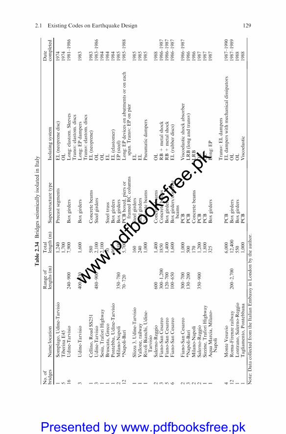
Table2.34
Bridges
seismicallyisolatedin
Italy
No.of
bridges
Name/location
Rangeof
lengths(m
)Total
length
(m)
Superstructure
type
Isolatingsystem
Date
completed
1Somplago,Udine-Tarvisio
1,240
Precastsegments
EL(neoprenedisc)
1974
5TiberinaE45
1,700
OL
1974
16
Udine-Tarvisio
240–900
7,900
Boxgirders
Long:elastom.Sleeves
1981–1986
Transv:elastom.discs
3Udine-Tarvisio
400–830
1,600
Boxgirders
Long:EPdampers
1983
Transv:elastom.discs
1Cellino,RoadSS251
580
Concretebeams
EL(neoprene)
1983
3Udine-Tarvisio
480–900
2,100
Steelgirders
OL
1983–1986
1Sesia,TraforiHighway
2,100
OL
1984
1Bruscata,Greco
70
Steeltruss
EL
1984
1Pontebba,Udine-Tarvisio
960
Boxgirders
EL(elastomer)
1984
2Milano-N
apoli
350–780
1,100
Boxgirders
EP(steel)
1985
12
*Napoli-Bari
70–720
5,700
PCBboxed,piers
or
framed
RCcolumns
Long:EPdevices
onabutm
entsoroneach
span.Transv:EPonpier
1985–1988
1Slizza3,Udine-Tarvisio
160
Steelgirders
EL
1985
1Vallone,railway
240
Steelgirders
EL
1985
1RivoliBianchi,Udine-
Tarvisio
1,000
Concretebeams
Pneumaticdampers
1985
2Salerno-R
eggio
600
1,400
Concretebeams
OL
1988
3Fiano-SanCesareo
300–1,200
1850
Concretebeams
RB+
metalshock
1986–1987
5Fiano-SanCesareo
120–700
1,400
Boxgirders
RB+
metalshock
1986–1987
6Fiano-SanCesareo
100–650
1,600
Boxgirders/concrete
beams
EL(rubber
discs)
1986–1987
2Fiano-SanCesareo
300–700
1,000
PCB
Viscoelasticshock
absorber
1986–1987
3*Napoli-Bari
130–200
500
PCB
LRB(longandtransv)
1986
2Milano-N
apoli
170
Concretebeams
LRB
1986
2Salerno-R
eggio
350–900
1,200
PCB
OL
1987
1Sizzine,TraforiHighway
1,800
PCB
OL
1987
1AquaMarcia,Milano-
Napoli
325
Boxgirders
Long:EP
1987
Transv:ELdampers
4Monte
Vesuvio
6,000
PCB
ELdamperswithmechanicaldissipators
1987–1990
12
Roma-Firenze
railway
200–2,700
12,400
Boxgirders
OL
1987–1989
1Lontrano,Salerno-R
eggio
550
Boxgirders
OL
1988
1Tagliamento,Pontebbana
1,000
PCB
Viscoelastic
1988
Note:Data
collectedfrom
theItalianEmbassyin
Londonbytheauthor.
2.1 Existing Codes on Earthquake Design 129
www.pdfbo
oksfr
ee.pk
Presented by www.pdfbooksfree.pk
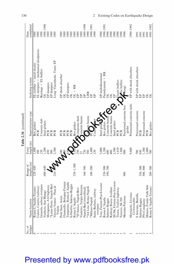
Table2.34
(continued)
No.of
bridges
Name/location
Rangeof
lengths(m
)Total
length
(m)
Superstructure
type
Isolatingsystem
Date
completed
6Roma-L’A
quila-Teramo
128–450
1,800
Boxgirders
EL(rubber
+metalshock)
1988
1Calore,Caserta(railway)
100
PCB
ELdampers+
mechanicaldissipators
1988
1Granola,railwayoverpass
120
Concreteslab
Bearings+
ELbuffers
1988
2Viaducts,SanMango
600–640
1,200
Steelgirders
OL
1988–1990
1Morignano,A14highway
450
PCB
EPdampers
1989
1*Lenze-Pezze,Napoli-Bari
300
PCB
EPdampers
1989
2VittorioVeneto–Piandi
Vedoia
210–2,100
2,300
PCB
Long:Viscoelastic.Trans:EP
1989
1PontSuaz,Aosta
240
PCB
EPshock
absorber
1989
1Flumicello,Bologna-Firenze
300
PCB
OL
1989
1Tem
perino,Roma-L’A
quila
830
PCB
EPdampers
1989
1S.O
nofrio,Salerno-R
eggio
450
PCB
OL
1989
3Roma-L’A
quila
230–1,300
1,800
Boxgirders
OL+
RB
1989
1*D’A
ntico,Napoli-Bari
250
Composite
deck
EP
1989
1Viadotto,Targia-Siracusa
23
Concretebeams
EP
1989
3Napoli-Bari(retrofitted)
160–390
720
PCB
EP
1989–1990
1*3rd
Line,Roma-N
apoli
580
Concretebeams
LRB
1990
7*Milano-N
apoli
100–200
1,000
PCB
EP
1990–1991
1Santa
Barbara,railway
overpass
120
Concreteslab
EP
1990
1Tora,Firenze-Pisa-Livorno
5,000
Steelgirders
EPmultidirectional
1990
3Roma-L’A
quila
230–500
1,200
Boxgirders
Pneudynamic+
RB
1990–1991
2Salerno-R
eggio
190,390
600
Concretebeams
OL
1990
1RailwayRoccaAvellino
400
Concretebeams
OL
1990
1SS206,F
irenze-Pisa-Livorno
2,500
Steelgirders
EP
1990
1Tiasca,Traforihighway
1,610
PCB
Elasticbuffers
1990
1Vesuvio,SS269
1,860
PCB
Elasticbuffers
1990
3Messina-Palerm
o900
900
Prestressed
concretebox
girder
EP(long)
1990
1Mortaiolo,Livorno-
Civitavecchio
9,600
Prestressed
concreteslabs
EPwithshock
absorbers
1990–1992
1SAntonio,Bretella
700
Prestressed
concrete
EPwithshock
absorbers
1991
2Salerno-R
eggio
350.500
850
PCB
EP
1991
2PN-C
onigliano
500,800
1,300
Prestressed
concrete
EP
1991
1Minuto,FondoValleSele
1,000
PCB
OL
1991
3Roma-L’A
quila-Teramo
200–300
700
Boxgirders
OL
1991–1992
130 2 Existing Codes on Earthquake Design
www.pdfbo
oksfr
ee.pk
Presented by www.pdfbooksfree.pk

Table2.34
(continued)
No.of
bridges
Name/location
Rangeof
lengths(m
)Total
length
(m)
Superstructure
type
Isolatingsystem
Date
completed
1Poggio
Ibem
a,Livorno-
Civitavecchia
2,500
PCB
OL
1991–1992
3Livorno-C
ecina
600–1800
2,800
PCB
EP,EP+
RB
1991–1992
1*Rumeano,Via
Salaria
340
PCB
EP
Retrofit
designed
1ViadottoNo2,Tangenziale
Potenza
240
PCB
EP
1990
1Angusta,Siracusa
450
Boxed
RCbeams
EL
1990
7*Salerno-R
Calabria
100–500
1,800
PCBwithconnectingslabs
EP
Retrofit
designed
1Fragneto
870
Steelboxgirder
withRC
slabs
EPdevices
onpiers,withSTlong.Highest
piers
connected
Designed
1Ponte
NelleAlpi,Via
Veneto-PiandiVedoia
310
Steelboxgirder
withRC
slabs
Long:EPwithST
Designed
Transv:EPonallpiers
Key:
EP=
Elastic–plasticbehaviour
EL=
Elastic
OL=
Oleodynamicsystem
(EPequivalent)
SL=
Slidingsupport
ST=
Shock
transm
ittersystem
associatedwithSL
RB=
Rubber
bearings
LRB=
Lead-rubber
bearings
RC=
Reinforced
concrete
PCB=
Prestressed
concretebeams
Notes:
Wherebridges
are
two-w
ay,they
havebeenregarded
asasinglebridgein
estimatingthelength.
Thetotallength
ofisolatedbridges
isthusgreaterthan100km.
Ofthemore
recentbridges
(1985–1992),typicaldesignvalues
oftheparametersare
Yield/w
eightratio:5–28%,witharepresentativevalueof10%
.�Maxim
um
seismicdisplacement:�30to�150mm,witharepresentativevalueof�60mm.
�Peakgroundacceleration:0.15�0.40g,witharepresentativevalueof0.25g.
Knownretrofitsare
indicatedwithanasterisk(*)
Inform
ationanddata
collectedfrom
theItalianEmbassyin
Londonbytheauthor.
Inform
ationcollectedfrom
ResearchLibrary,Westm
inster,Londonbytheauthor.
Researchdata
from
theResearchLibrary,Westm
inster,Londonbytheauthor.
Note:ResearchData
from
theTim
esdocumentsin
Westm
inster
ResearchLibrary,Londonbytheauthor.
2.1 Existing Codes on Earthquake Design 131
www.pdfbo
oksfr
ee.pk
Presented by www.pdfbooksfree.pk

Table2.35
Variousapplicationsandpossibilitiesofusingresponse-controlled
structuresin
buildings
Buildingapplication
Effect/technical
them
eHousing
Generaloffice
building
Publichigh-
rise
building
Disaster
preventive
building
Artgallery/
museums
facility
Atomicpower
facility
Hospitalfacility
Modern
industrial
facility
ab
cd
ef
gh
1.Ensure
safety
ofbuilding
structure
Safe
Safe
Safe
Safe
Safe
Safe
Safe
Safe
2.Freedom
indesignof
cross-section
ofmem
bers
Economy,
design
freedom
Economy,
design
freedom
3.Prevent
vibrations,
sliding,rolling
ofcontents
Safe
Satisfactory
perform
ance
Satisfactory
perform
ance
Satisfactory
perfor-
mance
Protect
the
exhibits
Protect
contents.
Satisfactory
perform
ance.
Prevent
hazardous
discharge
Protect
contents.
Satisfactory
perform
ance.
Prevent
hazardous
discharge
Satisfactory
perform
ance.
Prevent
hazardous
discharge
4.P
reventlossof
secondary
materials
Safe
economy,
design
freedom
Safe
economy,
design
freedom
Satisfactory
perform
ance
Satisfactory
perform
ance
Satisfactory
perform
ance
Satisfactory
perform
ance
Satisfactory
perform
ance
Satisfactory
perform
ance
5.Sensitivity
controlwhen
thevibrations
are
not
comfortable
Satisfactory
living
conditions
Satisfactory
living
conditions
Satisfactory
living
conditions
6.Maintain
proper
functioningof
machinery,
equipment,
etc.
Satisfactory
perform
ance
Satisfactory
perform
ance
Satisfactory
perform
ance
Note:They
are
collectedandthen
placedin
thecorrectorder
from
numerousliterature
onearthquakes
andbuildingsrelatedto
earthquakes.They
are
basedonconstructed
facilities.
132 2 Existing Codes on Earthquake Design
www.pdfbo
oksfr
ee.pk
Presented by www.pdfbooksfree.pk

Table2.36
Item
(0)Hachiya
Apartments
(1)ChristianData
Center
(2)Okumura
group
(3)ObayashiGroupTechnical
ResearchCenter
(4)Dieres
Industries
Fujizawasite
TC
wing
(5)Funab
ashi
TaketomoDorm
itory
(6)Okumura
Group
Designed
by
TokyoBuilding
ResearchCenter
TokyoBuilding
ResearchCenter,
Unitika
TokyoBuilding
ResearchCenter,
Okumura
group
Obayashigroup
Oires
Industries,
Symiono
Constructions,
YasuiBuilding
TakenakaKomyten
–
Design
requirem
ents
Antiseismic.Prevent
anydamageto
goodsstored
Antiseismic.Protect
computerandstored
data
fortechnical
Antiseismic.Protectionof
computerandother
laboratory
equipment
Designers
Safety
andfire
resistance
during
earthquak
e
–
No.offloors
+2
+2,–1
+4
No.offloors
+5
+5
+3
Built-up
area,m
260.18
226.21
348.18
Built-uparea,m
2351.92
1136.5
719.28
Application
Housing(residential
Data
house
Researchcenter
Application
Laboratory
Researchlaboratory
andoffice
Dorm
itory
Structure
RCCframe(shear
wall)
RCCframe(shear
wall)
RCCframe
Structure
RC
RC
RC
Foundation
Raftfoundationwith
castin
situ
piles
Deepfoundation
RCCcastin
situ
raft
Foundation
PHCtie(cem
ent
groutmethod)
Concretein
situ
raft
(each-drilling
method)
Concretein
situ
raft
(earth-drillingmethod)
Isolator:
Dim
ensions,
mm
82�
300dia
Rubber
5thick�
300
dia
(12layers)
Rubber
7thick�
500
dia
(14layers)
Isolator:Dim
ensions,mm
Rubber
4.4
thick
�740dia
(61
layers)
Rubber
10thick�
24
dia
(H=
363),OD
=650,700,750,
800)
Rubber
7thick�
670dia
(19layers)(H
=187)
Rubber
8thick�
700dia
(18layers)(H
=195)
Numbers
632
25
Numbers
14
35
14
Supporting
force
s=
45kg/cm
2,0.5
t/cm
(32t)
s=
60kg/cm
2,0.5
t/cm
(42.5t)
s=
60kg/cm
2,0.86t/
cm(120t)
Supportingforce
200t
200t!
6Nos.
150t!
8Nos.
Response-
control
device
Frictionforcebetween
PCplates
Usesplastic
deform
ationofsteel
bars
bentto
makea
loop(8
Nos.)
Usesplastic
deform
ationofsteel
bars
bentto
makea
loop(12Nos.)
Response-controldevice
Useselasto-
plastic
recoveryof
steelbars
(96
Nos.)
Leadpluginserted
inlaminatedrubber
Viscousdamper
(8Nos.)
Shearforce
coefficient
usedin
design
0.2
0.15
0.15
Shearforcecoefficientusedin
design
0.15
0.2
0.15
Fundamental
periodSmall
deform
ation
1.83s
14s
1.4
sFundamentalperiodSmall
deform
ation
X=
1.33s
X=
0.895s
X=
2.09s
Y=
1.24s
Y=
0.908s(at50%
deflection)
Y=
2.10s
Large
deform
ation
1.9
s2.1
sLargedeform
ation
X=
3.12s
X=
2.143s
Note:Data
collectedfrom
theBritish
Library
inLondonbytheauthorandplacedin
thegiven
order.
2.1 Existing Codes on Earthquake Design 133
www.pdfbo
oksfr
ee.pk
Presented by www.pdfbooksfree.pk

Table2.36
(continued)
Item
(0)Hachiya
Apartments
(1)ChristianData
Center
(2)Okumura
group
(3)ObayashiGroupTechnical
ResearchCenter
(4)Dieres
Industries
Fujizawasite
TC
wing
(5)Funabashi
TaketomoDorm
itory
(6)Okumura
Group
Y=
3.08s
Y=
2.148s(at100%
deflection)
Incident
seismicwave
ElCentro1940(N
S)
ElCentro1940(N
S)
ElCentro1940(N
S)
Incidentseismicwave
ElCentro1940
(NS)
ElCentro1940(N
S)
ElCentro1940(N
S)
Hachinohe1968(N
S)
Hachinohe1968(N
S)
Taft1952(EW)
Hachinohe1968
(NS)
Hachinohe1968(N
S)
Taft1952(EW)
Hachinohe1968(EW)
Taft1952(EW)
Hachinohe1968(N
S)
Hachinohe1968
(EW)
Hachinohe1968
(EW)
Tokyo1011956(N
S)
Taft1952(EW)
Taft1952(EW)
Taft1952(EW)
Hachinohe1968(N
S)
Man-m
ade
earthquake
twowaves
KT0081980(N
S)
Man-m
adeearthquak
efourwaves
Man-m
ade
earthquak
etw
owaves
Inputlevel
300gal
300gal,450gal
300gal,450gal
Inputlevel
25cm
/s,50cm
/s25cm
/s,50cm
/s25cm
/s,50cm
/s
Item
(6)Kashim
aConstructions
ResearchCenter,
NishiChofu
Acciystue
(7)ChristianData
Center(reapplied)
(8)Fukumiya
Apartments
(9)ShibuyaShim
izuBuildingNo.1
(10)Fujita
Industries,6th
Laboratory
(11)InorganicMaterials
ResearchCenter,
Vibration-FreeWing
12
34
56
7
Designed
by
Kashim
aConstructions
TokyoBuilding
ResearchCenter
Okumura
group
Obayashigroup
Fujita
Kogyo
SecretariatoftheMinistry
ofconstruction,
PlanningBureau
Design
requirem
ents
Reduce
seismicinput
andinsulate
(isolate)
from
Earth’s
vibrations
Anti-seism
ic.Prevent
anydamageto
storedgoods
Safety
ofbuilding.
Added
valuein
business
Protect
themain
buildingandOA
equipmentinstalledtherein
Protect
themain
buildingandthe
equipmentstoredthereinsuch
as
laboratory
equipmentandcomputers
Protect
themain
building
andresearchequipment
storedtherein
No.offloors
+2
+2
+4
+5,–2
+3
+1
Built-uparea,
m2
379.10
149.43
225.40
560.30
102.21
8,341(old
–7,725;new
–616)
Application
Researchlaboratory
Data
house
Cooperativehousing
Office
Researchlaboratory
Researchcenter
Structure
RC
RC
RC
RCC
RCC
RCC
134 2 Existing Codes on Earthquake Design
www.pdfbo
oksfr
ee.pk
Presented by www.pdfbooksfree.pk

Table2.36
(continued)
Item
(0)Hachiya
Apartments
(1)ChristianData
Center
(2)Okumura
group
(3)ObayashiGroupTechnical
ResearchCenter
(4)Dieres
Industries
Fujizawasite
TC
wing
(5)Funabashi
TaketomoDorm
itory
(6)Okumura
Group
Foundation
Concretein
situ
raft
(deepfoundation)
Deepfoundation
Concretein
situ
raft
(miniature
earth-
drillingmethod)
Concretein
situ
raft
(earth-drillingmethod)
PHCpile(typeA,B
)cementgroutmethod
PHCraft(typeA)
blastmethod
Isolator:
Dim
ensions,
mm
320�
1340(48thick�
5dia);308�
1080
(38thick�
6dia)
4thick�
435dia
(25
layers)
5.0
thick�
620dia
(50layers);6.0
thick�
740dia
(45layers)
4.0
thick�
450dia
(44layers)
3.2
thick�
420dia
(62layers)
Numbers
18
12
20
432
Supporting
force
165t:1340dia
s=
60kg/cm
2;0.55t/
cm(90t)
100-150t:620dia
65t(m
ax80t)
100t:1080dia
200-250t:740dia
Response-
control
device
Elasto-plasticdamper
usingmildsteelbars
(14Nos.)
Usesplastic
deform
ationofsteel
bars
bentto
makea
loop(6
Nos.)
Usesplastic
deform
ationofsteel
bars
bentto
makea
loop(7
Nos.)
Elasto-plasticdamper
usingmildsteelbars
(48Nos.)
Elasto-plasticdamper
usingmildsteel
bars
(108nos.)
Shearforce
coefficient
usedin
design
0.2
0.15
0.2
0.15:Basement,1stfloor;
0.183:3rd
floor
;0.205:5th
floor
0.15:1stfloor,
0.17:2ndfloor;
0.20:3rd
floor
0.15
Primary
period
Small
deform
ation
X=
0.828s
1.3
s1.4
sX=
1.30s
1.35s
X=
1.17s
Y=
0.809s
Y=
1.24s
Y=
1.17s
Large
deform
ation
1.80s
1.9
s2.2
sX=
2.99s
X=
2.26s
Y=
2.97s
Y=
2.26s
Incident
seismicwave
ElCentro
1940(N
S)
ElCentro
1940(N
S)
ElCentro
1940(N
S)
ElCentro
1940(N
S)
ElCentro1940(N
S)
ElCentro
1940(N
S)
Taft1952
(EW)
Taft1952(EW)
Taft1952(EW)
Taft1952(EW)
Taft1952(EW)
Taft1952(EW)
Tokyo101
1956(N
S)
Hachinohe
1968(N
S)
Tokyo101
1956(N
S)
Hachinohe1968(N
S)
Hachinohe1968(N
S)
Hachinohe
1968(N
S)
SendaiTHO38-1
1978(EW)
Hachinohe
1968(N
S)
Hachinohe
1968(EW)
Hachinohe
1968(EW)
Hachinohe
1968(EW)
Sdkanrig
Sdkantig
Sdansrig
9 = ;Man-madeseismic
waves
Artm
79L00
(seism
icwave)
Tsukuba
85
NS
Tsukuba
85
EW
Tsukuba
86
NS
Tsukuba
86
EW
9 > > = > > ;Observed
seismic
waves
Inputlevel
25cm
/s,50cm
/s300gal,450gal
25cm
/s,50cm
/s25cm
/s,50cm
/s25cm
/s,50cm
/s25cm
/s,50cm
/s
Notes:
Designersdata
collectedbytheauthorfrom
statedcompaniesin
Japan.
Data
collectedfrom
U.S.A
andJapanesereports,British
Library,Kingscross,Londonbytheauthor.They
are
placedunder
topics.
Data
collectedfrom
thecompaniesin
thereportsavailablewithBritish
Library,London.They
are
placedunder
topics.
2.1 Existing Codes on Earthquake Design 135
www.pdfbo
oksfr
ee.pk
Presented by www.pdfbooksfree.pk
evaluated. The spectral acceleration level is about the same in all codes men-tioned here. The velocity versus coverage (average) was taken by Soong et al.to be 210 m/s.
Data on Constructed Facilities
Some constructed building and other structural facilities have been examinedwith respect to the usage of seismic devices and are categorized on the basis ofthe types of structures and seismic devices installed to control and minimizevarious parameters inclusive of disastrous vibrations included by the earth-quakes. Tables (2.34) to (2.36) give the details of the constructed facilities wherevarious devices have been installed.
Bibliography
Abe, M., and Fujino, Y. Dynamic characteristics of multiple tuned mass dampers and somedesign formulas. Earthquake Eng. Struct. Dyn. 1994; 23(8), 813–836.
Algeria RPA (1999) Algerian EarthquakeResistant Regulation-Document Technique, Regle-mentaire (DTR) 1982
Argentina INPRESS-CIROSC 103 (1991) -Australian standard AS1170-4-1993 MinimumDesign Roads on structures Pa A4, Earthquake loads 1996
Australia AS I 1704 (1993) -Australian standard AS1170-4-1993 Minimum Design Roads onstructures Pa A4, Earthquake loads 1996
Beliayev, V.S., Vinogradov, V.V., and Guskov, V.D. Most recent development of the studiesfor seismic isolation of nuclear structures in Russia, International Post-Smirt ConferenceSeminar on Seismic Isolation, Passive Energy Dissipation and Control of Vibrations ofStructures, Santiago, Chile, 1995.
Bishop, R.E.D. and Welbourn, D.B. The problem of the dynamic vibration absorber.Engineering, London, 1952, 174, 769.
Brock, J.E. A Note on the Damped Vibration Absorber. J. Appl. Mech. 13(4), A-284.Carter, W.J., and Lin, F.C. Steady-state behavior of nonlinear dynamic absorber. J. Appl.
Mech. 1961; 60-WA-14, 67–70.Chang, J.C.H., and Soong, T.T. Structural control using active tuned mass dampers. J. Eng.
Mech. Div. ASCE 1980; 106(EM6): 1091–1098.China T J 11-78 and GB J11-89Chowdhury, A.H., Iwuchukwu, M.D., and Garske, J.J. The Past and Future of Seismic
Effectiveness of Tuned Mass Dampers, Structural Control (Leipholz, H.H.E., ed.), Marti-nus Nijhoff Publishers, Dordrecht, 1987; 105–127.
Clarke, A.J. Multiple passive tuned mass damper for reducing earthquake induced buildingmotion, Proc. 9th Wld. Conf. Earthquake Eng., 5, Japan, 1988; 779–784.
Den Hartog, J.P. Mechanical Vibrations, 4th edition, McGraw-Hill, New York, 1956.Ding, J.H., and Ou, J.P. Theoretical study and performance experiment for cylinder with
holes viscous damper. World Inf. Earthquake Eng. 2001; 17(1): 30–35 (in Chinese).Englekirk, R., Seismic Design of Reinforcement and Precast Concrete Buildings. Wiley, New
York, 2003.ENR. Hancock Tower Now to Get Dampers, Engineering News-Record, Oct. 30, 1975; 11.ENR. Tower Cables Handle Wind, Water Tank Dampens It, Engineering News-Record,
Dec. 9, 1971; 23.Europ 1-1 OCT(94), Eurocode 8-Design provisions for Earthquake Resistance of structures
ENV 1994–1998
136 2 Existing Codes on Earthquake Design
www.pdfbo
oksfr
ee.pk
Presented by www.pdfbooksfree.pk

Fajfar, P. Equivalent ductility factors taking into account low-cycle fatigue. Earthquake Eng.Struct. Dyn. 1992, 21, 837–848.
Falcon, K.C., Stone, B.J., Simcock, W.D., and Andrew, C. Optimization of vibration absor-bers: A graphical method for use on idealized systems with restricting damping. J. Mech.Eng. Sci. 1967, 9, 374–381.
Frahm, H. Device for Damped Vibrations of Bodies, U.S. Patent No. 989958, Oct. 30, 1909.Fu, Y., and Kasai, K. Comparative study of frames using viscoelastic and viscous dampers. J.
Struct. Eng., Am. Soc. Civil Eng. 1998; 122(10), 513–522.Fujita, T. Studies about vibration isolating floor using pre-stretched or pre-compressed
springs (Part 2. Vibration characteristics and vibration isolator properties II.). SeisanKenkyu, December, 1980; 32(10), 28–31.
Fujita, T., Hattori, S., and Ishida, J. Studies about vibration isolating floor using pre-stretched or pre-compressed springs (Part 1. Vibration characteristics and vibration iso-lator properties I.). Seisan Kenkyu, August, 1980; 32(8), 48–51.
Fujita, T., Hattori, S., and Ishida, J. Studies about vibration isolating floor using pre-stretched or pre-compressed springs (Part 3. Vibration characteristics and vibration iso-lator properties III.). Seisan Kenkyu, December, 1980; 32(12), 22–25.
Furukawa, Y., Kawaguchi, S., Sukagawa, M., Masaki, N., Sera, S., Kato, N., Washiyama, Y.,and Mitsusaka, Y. Performance and quality control of viscous dampers. Proc.Structural Engineers World Congress (SEWC), Yokohama, JAPAN, CD-Rom, T3-3-3,2002.
Garcia de Jalon, J., and Bayo, E. Kinematic and Dynamic Simulation of Multibody Systems:The Real Time Challenge. Springer, Berlin, 1994.
GB50011-2001. Code for Seismic Design of Buildings. China Building Industry Press, Beijing,China (in Chinese), 2001.
Housner, G.W. et al. Structural control: Past, present and future. J. Struct. Eng. ASCE 1997;123(9): 897–971.
India Pakistan Criteria for Earthquake Resistant designing structures fifth revision Part I IS1893 (Part 1) 2002
Iran ICSRD (1988) Iranian code for seismic design of Buildings 1988. Building Housingregional centre, Tehran.
Ishikawa, K., Okuma, K., Shimada, A., Nakamura, H., and Masaki, N. JSSI Manual forBuilding Passive Control Technology: Part-5 Performance and Quality Control of Visco-elastic Dampers (Companion Paper, Presented at 13WCEE).
ISO3010: 1988 Base for design of structures_Seismic Actions on Structures. Notification ofNo.1446 of Ministry of Construction, Japan/May 31, 2000. Notification of No.2009 ofMinistry of Construction, Japan/May 31, 2000
Israel IC-413 (1994) SI 413Design provision for EarthquakeResistant of structures. StandardInstitute of Israel 1988.
Italy CNR-GNDT (1986) & Eurocode Technical Rulers for Constructions in seismic zonesPublic works ministry 2000.
Iwan, W.D., and Gates, N.C. Estimating earthquake response of simple hysteretic structures.J. Eng. Mech. Div. ASCE 1979; 105(EM3): 391–405.
Izumi, M. Mitsuhashi, H., Sasaki, T., Katsukura, H., and Aizawa, F. Studies about dampingof vibrations in buildings. Basic studies about energy dissipation-type structure. NipponKecnchiku Gakkai, Tohoku-shibu, February, 1980; 85–88.
Jangid, R., and Londhe, Y. Effectiveness of elliptical rolling rods for base isolation. J. Struct.Eng. (ASCE) 1988; 124: 469–472.
Jangid, R.S. Response of pure-friction sliding structures to bi-directional harmonic groundmotion. Eng. Struct. 1997; 19: 97–104.
Jangid, R.S. Seismic response of sliding structures to bi-directional earthquake excitation.Earthquake Eng. Struct. Dyn. 1996; 25: 1301–1306.
Bibliography 137
www.pdfbo
oksfr
ee.pk
Presented by www.pdfbooksfree.pk

Japan BLEO (1981) Part 1, Earthquake Resistant Design of Structures Part 2, EarthquakeResistant Design of Building (Tokyo Japan, 2000)
JSSI Manual. Design and Construction Manual for Passively Controlled Buildings, JapanSociety of Seismic Isolation (JSSI), First Edition, Tokyo, JAPAN, October (in Japanese,405 pages), 2003.
Kanada, M., Kasai, K., and Okuma, K. Innovative passive control scheme: a Japanese12-story building with stepping columns and viscoelastic dampers. Proc. Structural Engi-neers World Congress (SEWC), Yokohama, JAPAN, CD-ROM, T2-2-a-5, 2002.
Kasai, K., and Kibayashi, M. JSSI Manual for Building Passive Control Technology, Part-1Manual Contents and Design Analysis Methods’’, 13WCEE, No.2989, 2004.
Kasai, K., and Kibayashi, M. JSSI Manual for Building Passive Control Technology: Part-1Control Device and System (Companion Paper, Presented at 13WCEE).
Kasai, K., and Nishimura, T. Equivalent linearization of passive control system having oildamper bi-linearly dependent on velocity. J. Struct. Constr. Eng. (Transaction of AIJ),(in Review), (in Japanese), 2004.
Kasai, K., and Okuma, K. Accuracy enhancement of Kelvin-type modeling for linear viscoe-lastic dampers. A refined model including effect of input frequency on, 2002
Kasai, K., and Okuma, K. Kelvin-type formulation and its accuracy for practical modeling oflinear viscoelastic dampers (Part1: One-Mass SystemHaving Damper and Elastic / Inelas-tic Frame). J. Struct. Constr. Eng. (Transactions of AIJ), No. 550, 2001; 71–78, Dec.(in Japanese).
Kasai, K., Ito, H., andWatanabe, A. Peak response prediction rule for a SDOF elasto-plasticsystem based on equivalent linearization technique. J. Struct. Constr. Eng. (Transactionsof AIJ), No. 571, 2003; 53–62, Sep. (in Japanese).
Kasai, K., Kibayashi, M., Takeuchi, T., Kimura, Y., Saito, Y., Nagashima, I., Mori, H.,Uchikoshi, M., Takahashi, O., and Oohara, K. Principles and current status of manual fordesign and construction of passively-controlled buildings: Part-1: Background scope, anddesign concept. Proc. Structural Engineers World Congress (SEWC), Yokohama,JAPAN, CD-ROM, T2-2-a-1, 2002.
Kasai, K., Suzuki, A., and Oohara, K. Equivalent linearization of a passive control systemhaving viscous dampers dependent on fractional power of velocity. J. Struct. Constr. Eng.(Transactions of AIJ), No. 574, 2003; 77–84, Dec. (in Japanese).
Kibayashi, M., Kasai, K., Tsuji, Y., Kato, S., Kikuchi, M., Kimura, Y., and Kobayashi, T.Principles and current status of manual for design and construction of passively-controlledbuildings: Part-2: JSSI Criteria for Implementation of Energy Dissipation Devices. Proc.Structural Engineers World Congress (SEWC), Yokohama, JAPAN, CD-ROM, T3-3-1,2002.
Kibayashi, M., Kasai, K., Ysuji, J., Kukuchi, M., Kimura, Y., Kobayashi, T., Nakamura, J.,and Matsubsa, Y. JSSI Manual for Building Passive Control Technology, Part-2 Criteriafor Implementation of Energy Dissipation Devices, 13WCEE, No. 2990, 2004.
Kobori, T, and Minai, R., Analytical study on active seismic response control: Seismic-response-controlled structure 1. Trans. Architectural Inst. Japan 1960; 66: 257–260 (inJapanese).
Kobori, T, and Minai, R., Condition for active seismic response control: seismic-response-controlled structure 2. Trans. Architectural Inst. Japan 1960; 66: 253–256 (in Japanese).
Kobori, T. Quake resistant and nonlinear problems of the structural vibrations to violentearthquake. J. Kyoto University Disaster Prevention Laboratory, 5th Anniversary Edition1956; 116–124 (in Japanese).
Kobori, T. The direction of earthquake resistant engineering. J. Architecture Building Sci.1958; 73: 5–9 (in Japanese).
Kobori, T., Koshika,N.Yamada, K., and Ikeda, Y. Seismic-response-controlled structure withactive mass driver system. Part 1: Design. Earthquake Eng. Struct. Dyn. 1991; 20: 133–149.
138 2 Existing Codes on Earthquake Design
www.pdfbo
oksfr
ee.pk
Presented by www.pdfbooksfree.pk

Kobori, T., Koshika, N. Yamada, K., and Ikeda, Y. Seismic-response-controlled structurewith active mass driver system. Part 2: Verification, Design. Earthquake Eng. Struct. Dyn.1991; 20: 151–166.
Krieg, R.D., and Krieg, D.N. Accuracy of numerical solution methods for the elastic,perfectly plastic model. Pres. Ves. Technol. 1997; 99: 510–515.
Kumaya, K., Arano, T., Kurihara,M., and Sasai, H. Structure incorporating sliding elementsand rubber in the foundations of buildings (Part 2. Rocking vibrations developed in avibration isolator structure developed at the time of sliding). Nippon Kikai Gakkai KoenRonbun-shu, No. 800–3, 1980; 89–91.
Kumaya, K., Arano, T., Kurihara,M., Sasai, H. Structure incorporating sliding elements andrubber in the foundations of buildings (Part 2. Methods of response analysis in a multi-freedom systems and comparison with experimental findings). Nippon Kikai Gakkai KoenRonbun-shu, No. 800–3, 1980; 92–94.
Li, Z., Rossow, E.C., and Shah, S.P. Sinusoidal forced vibration of sliding masonry system.Struct. Eng. ASCE 1989; 115: 1741–1755.
Liaw, T.C., Tian, Q.L., and Cheung, Y.K., Structures on sliding base subjected to horizontaland vertical motions. Struct. Eng. ASCE 1988; 114: 2119–2129.
Lin, B.C., and Tadjbakhsh, I.G. Effect of vertical motion on friction driven systems. Earth-quake Eng. Struct. Dyn. 1986; 14: 609–622.
Lin, T.W., Chern, C.C., and Hone, C.C. Experimental study of base isolation by free rollingrods. Earthquake Eng. Struct. Dyn. 1995; 24: 1645–1650.
Lu, L.Y., and Yang, Y.B. Dynamic response of equipment in structures with sliding support.Earthquake Eng. Struct. Dyn. 1997; 26: 61–77.
Makris, N., Dargush, G.F., and Constantinou, M.C. Dynamic analysis of viscoelastic fluiddampers. J. Eng. Mech. ASCE, 1995; 121(10), 1114–1121.
Masri, S.F., Bekey, G.A., and Caughey, T.K. On-line control of nonlinear flexible structures.J. Appl. Mech. ASME 1982; 49: 877–884.
Mathworks, Inc., MATLAB, Reference Guide. Natick, MA, 1999.Matsushita, S., Nomura, M., and Sasaki, T. Recovery properties of steel pipe type response-
control device. Nippon Kenchiku Gakkai, Tohoku-shibu, March, 1980; 129–132.Mexico UNAM (1983) M111 (1988)Miyazaki, N., and Mitsusaka, Y. Design of a building with 20% or greater damping, Tenth
World Conf. Earthquake Eng., Madrid, 1992; 4143–4148.Mokha, A., Constantinou, M.C., and Reinhorn, A.M. Verification of friction model of
Teflon bearings under triaxial load. Struct. Eng. ASCE 1993; 119: 240–261.Mori, M., Arano, T., Kataoka, T., Ochiai, K., and Sasai, H. Structure incorporating sliding
elements and rubber in the foundations of buildings (Part 1). Nippon Kikai Gakkai KoenRonbun-shu, No. 800–3, 1980; 88–91.
Mostaghel, N., and Khodaverdian, M. Dynamics of resilient-friction base isolator (R-FBI).Earthquake Eng. Struct. Dyn. 1987; 15: 379–390.
Mostaghel, N., and Tanbakuchi, J. Response of sliding structures to earthquake supportmotion. Earthquake Eng. Struct. Dyn. 1983; 11: 729–748.
Mostaghel, N., Hejazi, M., and Tanbakuchi, J. Response of sliding structure to harmonicsupport motion. Earthquake Eng. Struct. Dyn. 1983; 11: 355–366.
Nakagawa, K., Watanabe, S., and Shimaguchi. S. Experimental studies about dynamic floorsystem (Part 2) – Vibration experiment with a computer using vibration table.Dairin-gumigijutsu Kenkyusho-ho, No. 17, 1978; 17–21.
Nakata, Y. Performance and quality control of steel hysteretic damper. Proc. StructuralEngineers World Congress (SEWC), Yokohama, Japan, CD-ROM, T3-3-5, 2002.
Nakata, Y., Hirota, M., Shimizu, T., and Iida, T. JSSI manual for building passive controltechnology: Part-6 performance and quality control of steel dampers (Companion Paper,Presented at 13WCEE).
Bibliography 139
www.pdfbo
oksfr
ee.pk
Presented by www.pdfbooksfree.pk

New Zealand NZS 4203 (1992) and NZNSEE (1988) general structures designs, designloading for buildings. Standards association of New Zealand 2004.
Nishitani, A. Application of active structural control in Japan. Prog. Struct. Eng. Mater.1998; 1(3): 301–307.
Niwa, N., Kobori, T., Takahashi, M., Hatada, T., Kurino, H., and Tagami, J. Passive seismicresponse controlled high-rise building with high damping device. Earthquake Eng. Struct.Dyn. 1995, 24, 655–671.
Okuma, K., Ishikawa, K., Oku, T., Sone, Y., Nakamura, H., and Masaki, N. Performanceand quality control of viscoelastic dampers. Proc. Structural Engineers World Congress(SEWC), Yokohama, Japan, CD-ROM, T3-3-4, 2002.
Okuma, K., Kasai, K., and Tokoro, K. JSSI manual for building passive control technology:Part-10 time-history analysis model for viscoelastic dampers (Companion Paper, Pre-sented at 13WCEE), 2002.
Oldham, K.B., and Spanier, J. The Fractional Calculus. Academic Press, New York, 1974.Ooki, Y., Kasai, K., and Amemiya, K. JSSI manual for building passive control technology:
Part-11 Time-history Analysis Model for Viscoelastic Dampers Combining Iso-Butyleneand Stylene Polymers (Companion Paper, Presented at 13WCEE).
Ou, J.P., and Zou, X. Experimental study on properties of viscoelastic damper. J. VibrationShock 1999; 18(3): 12–19 (in Chinese).
Ou, J.P., He, Z., Wu, B., and Long, X. Seismic damage performance design for RC structures.J. Building (in Chinese), 2001; 21:1, 63–73.
Ou, J.P., Niu, D., and Wang, G. Seismic damage estimation and optimal design of nonlinearRC structures. J. Civil Eng. (in Chinese), 1993; 26:5, 14–21.
Ou, J.P., Wu, B., and Long, X. Parameter analysis of passive energy dissipation systems.Earthquake Eng. Vibration 1998; 18(1): 60–70 (in Chinese).
Park, Y.J., and Ang, A. H.-S. Mechanistic seismic damage model for reinforced concrete. J.Struct. Eng. 1985; 111(4): 722–739.
Pekcan, G., Mander, J.B., and Chen, S.S. The seismic response of a 1:3 scale model R.C.structure with elastomeric spring dampers. Earthquake Spectra, 1995; 11(2), 249–267.
Press, W.H., Teukolsky, S.A., Vetterling, W.T., and Flannery, B.P. Numerical recipes inFORTRAN, Cambridge University Press, Cambridge, UK, 1992.
Petersen et al. Dynamic analysis with tuned mass dampers private communication (Tworeports 1995).
Qumaroddin, M., Rasheedazzafar, Arya, A.S., and Chadra, B. Seismic response of masonrybuildings with sliding substructure. Struct. Eng. ASCE 1986; 112: 2001–2011.
Reinhorn, A.M., and Li, C. Experimental and analytical investigation of seismic retrofit ofstructures with supplemental damping, Part III: Viscous Damping Walls, TechnicalReport NCEER-95-0013, National Centre for Earthquake Engineering Research, Buf-falo, NY, 1995.
Reinhorn, A.M., Li, C., andConstantinou,M.C. Experimental and analytical investigation ofseismic retrofit of structures with supplemental damping, Part I: Fluid Viscous DampingDevices, Technical Report NCEER-95-0001, National Centre for Earthquake Engineer-ing Research, Buffalo, NY, 1995.
Schwahn, K.J., andDelinic, K. Verification of the reduction of structural vibrations bymeansof viscous dampers, Seismic Engineering, ASME, Pressure Vessel and Piping Conf.,Pittsburgh, PA, 1988, 144, 87–95.
Sekiguchi, Y., Kasai, K., and Ooba, K. JSSI manual for building passive control technology:Part-13 Time-history Analysis Model for Viscous Dampers (Companion Paper, Presentedat 13WCEE).
Sekiguchi, Y., Kasai, K., and Takahashi, O. JSSI manual for building passive controltechnology: Part-12 time-history analysis model for nonlinear oil dampers. (CompanionPaper, Presented at 13WCEE).
140 2 Existing Codes on Earthquake Design
www.pdfbo
oksfr
ee.pk
Presented by www.pdfbooksfree.pk

Shames, I.H., and Dym, C.L. Energy and Finite Element Methods in Structural Mechanics.Hemisphere Publishing, New York, 1985.
Shimazu, T., and Hidco, A. Basic experimental studies on vibration isolator properties oflayered walls. Nippn Kenchiku Gakkai Taikai, September, 1980; 755–757.
Soong, T.T., andDargush, G.F.Passive EnergyDissipation Systems in Structural Engineering.Wiley, New York, 1997.
Spencer Jr. B.F., and Sain, M.K. Controlling buildings: A new frontier in feedback. IEEEControl SystemsMagazine: Special Issue on Emerging Technologies (Samad, T. Guest ed.),1997; 17(6): 19–35.
Suresh, S. Fatigue of Materials. Cambridge University Press, Cambridge, 1991.Tanaka, K., Kawagushi, S., Sukagawa, M., Masaki, N., Sera, S., Washiyama, Y., and
Mitsusaka, Y. JSSI manual for building passive control technology: Part-4 Performanceand Quality Control of Viscous Dampers (Companion Paper, Presented at 13WCEE).
Taylor, D.P., and Constantinou, M.C. Fluid dampers for applications of seismic energydissipation and seismic isolation. Proceedings of the Eleventh World Conference onEarthquake Engineering, Acapulco, Mexico, 1996.
Tezcan, S., and Civi, A. Reduction in Earthquake Response of Structures by Means ofVibration Isolators, Proc. Second U.S. National Conf. on Earthquake Engrg., Earth-quake Engrg. Research Institute, Stanford Univ., California, 1979; 433–442.
Tsopelas, P., and Constantinou, M.C. NCEER-Taisei Corporation Research Program onSliding Seismic Isolation Systems for Bridges: Experimental and Analytical Study of aSystem Consisting of Sliding Bearings and Fluid Restoring Force/Damping Devices,Technical Report NCEER-94-0014, National Centre for Earthquake EngineeringResearch, Buffalo, NY, 1994.
Tsuyuki, Y., Kamei, T., Gofuku, Y., Iiyama, F., and Kotake, Y. Performance and qualitycontrol of oil-damper. Proc. Structural Engineers World Congress (SEWC), Yokohama,Japan, CD-ROM, T3-3-2, 2002.
Tsuyuki, Y., Kamei, T., Gofuku, Y., Kotake, Y., and Iiyama, F. JSSI manual for buildingpassive control technology: Part-3 Performance and Quality Control of Oil Dampers(Companion Paper, Presented at 13WCEE).
USA UBC. 95 (1995) 2 SEAOC (1990) ASCE Minimum Design Loads for Buildings andother structures, ASCE, USA.
Vidic, T., Fajfar, P., and Fischinger, M. Consistent inelastic design spectra: Strength anddisplacement. Earthquake Eng. Struct. Dyn. 1992; 23: 507–521.
Warburton, G.B., and Soni, S.R. Errors in response calculations for non-classically dampedstructures. Earthquake Eng. Struct. Dyn. 1977, 5, 365–376.
Westermo, B., and Udwadia, F., Periodic response of a sliding oscillator system to harmonicexcitation. Earthquake. Eng. Struct. Dyn. 1983; 11: 135–146.
Yang, J.N. Application of optimal control theory to civil engineering structures. J. Eng.Mech. Div. ASCE 1975; 101(6): 819–838.
Yang, Y.B., Lee, T.Y., and Tsai, I.C. Response of multi-degree-of-freedom structures withsliding supports. Earthquake Eng. Struct. Dyn. 19, 739–752, 1990
Yao, J.T.P. Concept of structural control. J. Struct. Div. ASCE 1972; 98(ST7): 1567–1574.Yasui, H., and Iniwa, C. Experimental studies about dynamic floor system (Part1) – Sinusoi-
dal forced damped vibration experiment on a large-scale model. Dairin-gumi GijutsuKenkyusho-ho, No. 16, 1978; pp. 46–50.
Yasunishi, K., and Tada, H. Discussions about aseismic isolator (steel, rubber laminationpad). Nippon Kenchiku Gakkai Taikai, September, 1980; 751–753.
Younis, C.J., and Tadjbakhsh, I.G. Response of sliding structure to base excitation. Eng.Mech. ASCE 1984; 110: 417–432.
Bibliography 141
www.pdfbo
oksfr
ee.pk
Presented by www.pdfbooksfree.pk

www.pdfbo
oksfr
ee.pk
Presented by www.pdfbooksfree.pk
Chapter 3
Basic Structural Dynamics
3.1 General Introduction
Most loads acting on structures are dynamic in origin. These loads can be
suddenly applied or allowed to reach full magnitude after a considerable
delay. On the other hand, the structures will have various degrees of freedomwith unclamped or clamped free or forced vibrations. These need to be dis-
cussed prior to the introduction of earthquake analysis and design.One of the most important applications of the theory of structural dynamics
is in analysing the response of structures to ground shaking caused by an
earthquake. In this chapter the reader can study the earthquake response oflinear SDF systems to earthquake motions. By definition, linear systems are
elastic systems and one shall also refer to them as linearly elastic systems toemphasize both properties. Because earthquakes can cause damage to many
structures, one is also interested in the response of yielding or inelastic systems,the subject is known as non-linear structural dynamics.
The later part of this chapter is concerned with the earthquake response
deformation, internal element forces, stresses and so on of simple structures asa function of time and how this response depends on the system parameters.
Then one introduces the response spectrum concept, which is central to earth-
quake engineering, together with procedures to determine the peak response ofsystems directly from the response spectrum. This is followed by a study of the
characteristics of earthquake response spectra, which lead into the design spec-
trum for the design of new structures and safety evaluation of existing structuresagainst future earthquakes. A number of examples are given to the reader in
order to understand the basis of structural dynamics in relation to earthquakes.
3.2 Structural Dynamics
3.2.1 General Introduction to Basic Dynamics
A number of textbooks and research papers have been written on the subject ofstructural dynamics in relation to earthquakes. Various mathematical models
M.Y.H. Bangash, Earthquake Resistant Buildings,DOI 10.1007/978-3-540-93818-7_3, � M.Y.H. Bangash 2011
143
www.pdfbo
oksfr
ee.pk
Presented by www.pdfbooksfree.pk
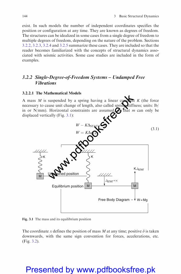
exist. In such models the number of independent coordinates specifies theposition or configuration at any time. They are known as degrees of freedom.The structures can be idealized in some cases from a single degree of freedom tomultiple degrees of freedom, depending on the nature of the problem. Sections3.2.2, 3.2.3, 3.2.4 and 3.2.5 summarize these cases. They are included so that thereader becomes familiarized with the concepts of structural dynamics asso-ciated with seismic activities. Some case studies are included in the form ofexamples.
3.2.2 Single-Degree-of-Freedom Systems – Undamped FreeVibrations
3.2.2.1 The Mathematical Models
A mass M is suspended by a spring having a linear constant K (the forcenecessary to cause unit change of length, also called spring stiffness; units: lb/in or N/mm). Horizontal constraints are assumed, so that m can only bedisplaced vertically (Fig. 3.1):
W� KDSTAT ¼ 0
W ¼ KDSTAT
(3:1)
The coordinate x defines the position of massM at any time; positive d is takendownwards, with the same sign convention for forces, accelerations, etc.
(Fig. 3.2).
Unstrained position
Free Body Diagram W = Mg
KΔSTAT
KK
M
M M
ΔSTAT = ×
Equilibrium position
Fig. 3.1 The mass and its equilibrium position
144 3 Basic Structural Dynamics
www.pdfbo
oksfr
ee.pk
Presented by www.pdfbooksfree.pk
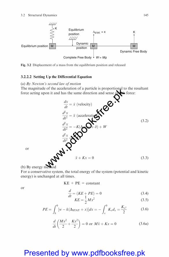
3.2.2.2 Setting Up the Differential Equation
(a) By Newton’s second law of motionThe magnitude of the acceleration of a particle is proportional to the resultantforce acting upon it and has the same direction and sense as this force:
dx
dt¼ _x ðvelocityÞ
d2x
dt2¼ €x ðaccelerationÞ
d2x
dt2¼ �KðDSTAT þ dÞ þW
d2x
dt2¼ �Kx
(3:2)
or
€xþ Kx ¼ 0 (3:3)
(b) By energy methodFor a conservative system, the total energy of the system (potential and kineticenergy) is unchanged at all times.
KE + PE = constantor
d
dt¼ ðKEþ PEÞ ¼ 0 (3:4)
KE ¼ 1
2Mx2 (3:5)
PE ¼Z 0
k
½w� kðDSTAT þ xÞ�dx ¼ �Z 0
x
Kxdx ¼Kx2
2(3:6)
d
dt
Mx2
2þ Kx2
2
� �¼ 0 or M€xþ Kx ¼ 0 (3:6a)
M MM
Equilibrium position
Dynamicposition
Complete Free Body W = Mg
Dynamic Free Body
KKΔSTAT. = x
Equilibrium position
Fig. 3.2 Displacement of a mass from the equilibrium position and released
3.2 Structural Dynamics 145
www.pdfbo
oksfr
ee.pk
Presented by www.pdfbooksfree.pk
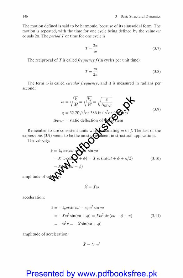
The motion defined is said to be harmonic, because of its sinusoidal form. Themotion is repeated, with the time for one cycle being defined by the value otequals 2p. The period T or time for one cycle is
T ¼ 2po
(3:7)
The reciprocal of T is called frequency f (in cycles per unit time):
T ¼ o2p
(3:8)
The term o is called circular frequency, and it is measured in radians persecond:
o ¼ffiffiffiffiffik
M
r¼
ffiffiffiffiffikgW
r¼
ffiffiffiffiffiffiffiffiffiffiffiffiffig
DSTAT
r
g ¼ 32:2ft=s2or 386 in= s2or 9:81m=s2
DSTAT ¼ static deflection of the system
(3:9)
Remember to use consistent units when calculating o or f. The last of theexpressions (3.9) seems to be the most convenient in structural applications.
The velocity:
_x ¼ _x0 cosot ¼ x0o sinot
¼ X o cosðotþ fÞ ¼ X o sinðotþ fþ p=2Þ
¼ _X cosðotþ fÞ
(3:10)
amplitude of velocity:
_X ¼ Xo
acceleration:
€x ¼ � _x0o sinot� x0o2 sinot
¼ �Xo2 sinðotþ fÞ ¼ Xo2 sinðotþ fþ pÞ
¼ �o2x ¼ � €X sinðotþ fÞ
(3:11)
amplitude of acceleration:
€X ¼ X o2
146 3 Basic Structural Dynamics
www.pdfbo
oksfr
ee.pk
Presented by www.pdfbooksfree.pk
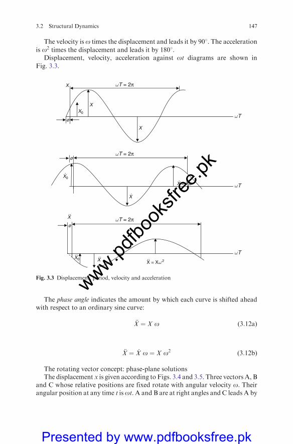
The velocity is o times the displacement and leads it by 908. The accelerationis o2 times the displacement and leads it by 1808.
Displacement, velocity, acceleration against ot diagrams are shown in
Fig. 3.3.
The phase angle indicates the amount by which each curve is shifted aheadwith respect to an ordinary sine curve:
€X ¼ X o (3:12a)
€X ¼ _X o ¼ X o2 (3:12b)
The rotating vector concept: phase-plane solutionsThe displacement x is given according to Figs. 3.4 and 3.5. Three vectors A, B
and C whose relative positions are fixed rotate with angular velocity o. Theirangular position at any time t isot. A and B are at right angles and C leads A by
X
XX0
ø
X ωT = 2π
ωT = 2π
ωT = 2π
ωT
ωT
ωT
X
ø
X0 ·
X = Xω
X
ø
X
X0 X = Xω 2
Fig. 3.3 Displacement, period, velocity and acceleration
3.2 Structural Dynamics 147
www.pdfbo
oksfr
ee.pk
Presented by www.pdfbooksfree.pk
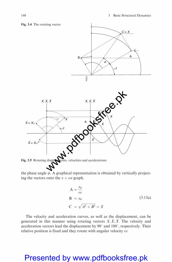
the phase angle f. A graphical representation is obtained by vertically project-
ing the vectors onto the xþ ot graph.
A ¼ x0o
B ¼ x0
C ¼ffiffiffiffiffiffiffiffiffiffiffiffiffiffiffiffiffiA2 þ B2
p¼ X
(3:13a)
The velocity and acceleration curves, as well as the displacement, can be
generated in this manner using rotating vectors X; _X; €X. The velocity and
acceleration vectors lead the displacement by 908 and 1808, respectively. Theirrelative position is fixed and they rotate with angular velocity o:
A
ωt
X, X, X
ω X
X = Xω2
X = Xω X
X
X
X, X, X
Fig. 3.5 Rotating displacements, velocities and accelerations
C = X
ω
AB
ωt
ø
2π
Fig. 3.4 The rotating vector
148 3 Basic Structural Dynamics
www.pdfbo
oksfr
ee.pk
Presented by www.pdfbooksfree.pk
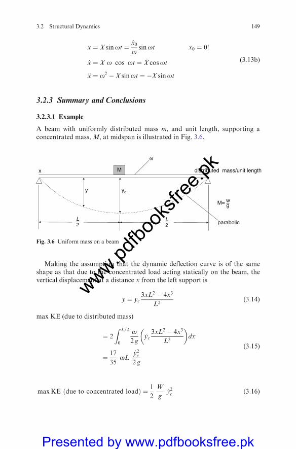
x ¼ X sinot ¼ _x0o
sinot x0 ¼ 0!
_x ¼ X o cos ot ¼ _X cosot
€x ¼ o2 � X sinot ¼ �X sinot
(3:13b)
3.2.3 Summary and Conclusions
3.2.3.1 Example
A beam with uniformly distributed mass m, and unit length, supporting aconcentrated mass, M, at midspan is illustrated in Fig. 3.6.
Making the assumption that the dynamic deflection curve is of the sameshape as that due to the concentrated load acting statically on the beam, thevertical displacement at a distance x from the left support is
y ¼ yc3xL2 � 4x3
L2(3:14)
max KE (due to distributed mass)
¼ 2
Z L=2
0
o2 g
_yc3xL2 � 4x3
L3
� �dx
¼ 17
35oL
_y2c2 g
(3:15)
maxKE ðdue to concentrated loadÞ ¼ 1
2
W
g_y2c (3:16)
M
y yc
x
ω
parabolic
distributed mass/unit length
2L
2L
M= gw
Fig. 3.6 Uniform mass on a beam
3.2 Structural Dynamics 149
www.pdfbo
oksfr
ee.pk
Presented by www.pdfbooksfree.pk
maxSE ¼ 12Ky2c
total energy ¼ KEþ SE ¼ constant(3:17)
¼ 1
2_y2c
Wþ 17
35oL
� �
gþ 1
2Ky2c ¼ constant (3:18)
@
@t¼ _yc
Wþ 17
35oL
g€yc þ Kyc
0B@
1CA ¼ 0 (3:19)
This expression is equivalent to (3.7) except that 1735 of the total mass of the
beam is lumped with the concentrated mass. The natural frequency is
f ¼ 1
2p
ffiffiffiffiffiffiffiffiffiffiffiffiffiffiffiffiffiffiffiffiffiffiffiKg
Wþ 17
35oL
vuut ¼ 1
2p
ffiffiffiffiffiffiffiffiffiffiffiffiffig
DSTAT
r(3:20)
where DSTAT is the static deflection under the concentrated load due to a totalload of Wþ 17
35oL acting at the same point.
3.2.3.2 Estimate of the Fundamental Frequency of Multi-mass Systems
by Rayleigh’s Method
The mass of the beam or structure is assumed negligible or is ‘‘lumped’’ asin (3.20).
Assume again that the dynamic amplitude of the loads W1;W2; . . . ;Wn isapproximated by the static deflections of the structure y1; y2; . . . ; yn at the loadpoints. Substitute into (3.16), remembering that the amplitude of the velocity is
_yi ¼ oy
max SE ¼XWiyi
2by Clapeyron’s theorem
(3:21)
maxKE ¼XMiy
2i
2at the equilibrium position
¼XMiy
21
2¼XMio2y2i
2¼ o2
g
PWiy
2i
2
(3:22)
XWiyi2¼ o2
g
XWiy2i
2(3:23)
150 3 Basic Structural Dynamics
www.pdfbo
oksfr
ee.pk
Presented by www.pdfbooksfree.pk
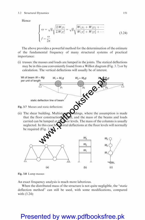
Hence
o ¼ ffiffiffigp
ffiffiffiffiffiffiffiffiffiffiffiffiffiffiSWiyi
SWiy2i
s¼ ffiffiffi
gp
ffiffiffiffiffiffiffiffiffiffiffiffiffiffiffiffiffiffiffiffiffiffiffiffiffiffiffiffiffiffiffiffiffiffiffiffiffiffiffiffiW1y1 þW2y2 þ � � �W1y
21 þW2y
22 þ � � �
s
f ¼ o2p
8>>><>>>:
(3:24)
The above provides a powerful method for the determination of the estimateof the fundamental frequency of many structural systems of practicalimportance:
(i) trusses: the masses and loads are lumped in the joints. The statical deflectionsmay be in this case conveniently found from aWilliot diagram (Fig. 3.7) or bycalculation. The vertical deflections will usually be of interest.
(ii) The shear building. Multistorey buildings, where the assumption is madethat the floor construction is rigid, and the mass of the beams and loadscarried can be lumped at the floor levels. The mass of the columns is usuallyneglected. In this case horizontal deflections at the floor levels will normallybe required (Fig. 3.8).
An exact frequency analysis is much more laborious.When the distributed mass of the structure is not quite negligible, the ‘‘static
deflection method’’ can still be used, with some modifications, compared
with (3.24):
W1
W2
W3
M1
M2
M3
(a) (b) (c)
Fig. 3.8 Lump masses
W1 = M1g W3 = M3gW2 = M2g
y1 y2 y3
Wt of beam W = Mgper unit of length
static deflection line of beam
Fig. 3.7 Masses and static deflections
3.2 Structural Dynamics 151
www.pdfbo
oksfr
ee.pk
Presented by www.pdfbooksfree.pk
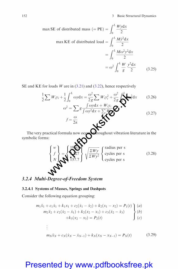
maxSE of distributed mass ð¼ PEÞ ¼Z L
0
Wydx
2
maxKE of distributed load ¼Z L
0
M _y2dx
2
¼Z L
0
Mo2y2dx
2
¼ o2
Z L
0
W
g
y2dx
2 (3:25)
SE and KE for loads W are in (3.21) and (3.22), hence respectively
1
2
XWiyi þ
1
2
Z L
0
oydx ¼ o2
2 g
XWiy
2i þ
o2
2 g
Z L
0
oy2i dx (3:26)
o2 ¼X
g
RoydxþWiyiR
oy2dxþP
Wiy2i
f ¼ o2p
(3:27)
The very practical formula now occurs throughout vibration literature in thesymbolic forms:
w
f
N
8><>:
9>=>; ¼
19:65
3:127
157:7
8><>:
9>=>;
ffiffiffiffiffiffiffiffiffiffiffiffiffiSWy
SWy2
s radius per s
cycles per s
cycles per s
8<: (3:28)
3.2.4 Multi-Degree-of-Freedom System
3.2.4.1 Systems of Masses, Springs and Dashpots
Consider the following equation grouping:
m1€x1 þ c1 _x1 þ k1x1 þ c2ð _x1 � _x2Þ þ k2ðx1 � x2Þ ¼ P1ðtÞm2€x2 þ c2ð _x2 � _x1Þ þ k2ðx2 � x1Þ þ c3ð _x2 � _x3Þ
þk3ðx2 � x3Þ ¼ P2ðtÞ
9>=>;ðaÞðbÞðcÞ
..
.
mN€xN þ cNð _xN � _xN�1Þ þ kNðxN � xN�1Þ ¼ PNðtÞ (3:29)
152 3 Basic Structural Dynamics
www.pdfbo
oksfr
ee.pk
Presented by www.pdfbooksfree.pk
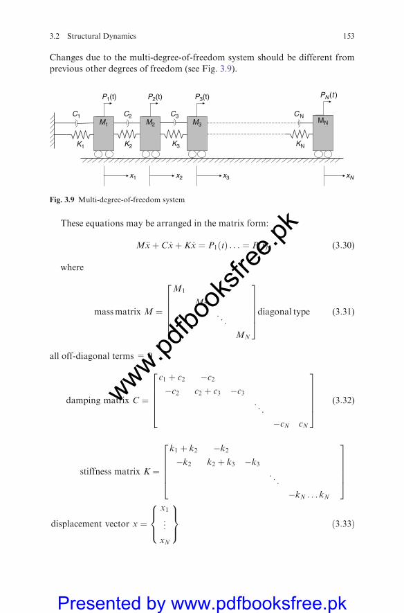
Changes due to the multi-degree-of-freedom system should be different from
previous other degrees of freedom (see Fig. 3.9).
These equations may be arranged in the matrix form:
M€xþ C _xþ K _x ¼ P1ðtÞ . . . ¼ PðtÞ (3:30)
where
massmatrix M ¼
M1
M2
. ..
MN
266664
377775diagonal type (3:31)
all off-diagonal terms = 0
damping matrix C ¼
c1 þ c2 �c2�c2 c2 þ c3 �c3
. ..
�cN cN
266664
377775 (3:32)
stiffness matrix K ¼
k1 þ k2 �k2�k2 k2 þ k3 �k3
. ..
�kN . . . kN
266664
377775
displacement vector x ¼x1
..
.
xN
8><>:
9>=>; ð3:33Þ
M1 M3M2MN
K1 K2 K3 KN
C1 C2 C3 CN
x1 x2 x3 xN
P1(t) P2(t) P3(t) PN(t )
Fig. 3.9 Multi-degree-of-freedom system
3.2 Structural Dynamics 153
www.pdfbo
oksfr
ee.pk
Presented by www.pdfbooksfree.pk
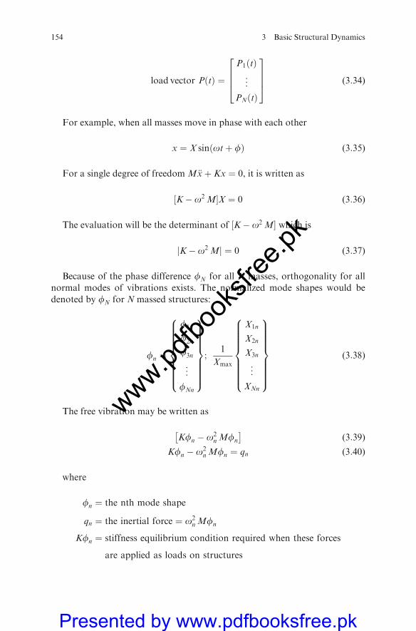
load vector PðtÞ ¼
P1ðtÞ...
PNðtÞ
2664
3775 (3:34)
For example, when all masses move in phase with each other
x ¼ X sinðotþ fÞ (3:35)
For a single degree of freedom M€xþ Kx ¼ 0, it is written as
½K� o2M�X ¼ 0 (3:36)
The evaluation will be the determinant of ½K� o2 M� which is
jK� o2Mj ¼ 0 (3:37)
Because of the phase difference fN for all N masses, orthogonality for all
normal modes of vibrations exists. The normalized mode shapes would be
denoted by fN for N massed structures:
fn ¼
f1n
f2n
f3n
..
.
fNn
8>>>>>>><>>>>>>>:
9>>>>>>>=>>>>>>>;
;1
Xmax
X1n
X2n
X3n
..
.
XNn
8>>>>>>><>>>>>>>:
9>>>>>>>=>>>>>>>;
(3:38)
The free vibration may be written as
Kfn � o2n Mfn
� �(3:39)
Kfn � o2n Mfn ¼ qn (3:40)
where
fn ¼ the nth mode shape
qn ¼ the inertial force ¼ o2n Mfn
Kfn ¼ stiffness equilibrium condition required when these forces
are applied as loads on structures
154 3 Basic Structural Dynamics
www.pdfbo
oksfr
ee.pk
Presented by www.pdfbooksfree.pk
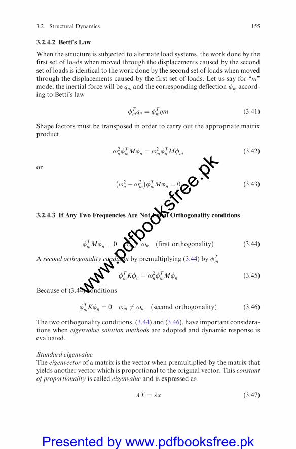
3.2.4.2 Betti’s Law
When the structure is subjected to alternate load systems, the work done by thefirst set of loads when moved through the displacements caused by the secondset of loads is identical to the work done by the second set of loads when movedthrough the displacements caused by the first set of loads. Let us say for ‘‘m’’mode, the inertial force will be qm and the corresponding deflection fm accord-ing to Betti’s law
fTmqn ¼ fT
mqm (3:41)
Shape factors must be transposed in order to carry out the appropriate matrixproduct
o2nf
TmMfn ¼ o2
mfTnMfm (3:42)
or
o2n � o2
m
� �fTmMfn ¼ 0 (3:43)
3.2.4.3 If Any Two Frequencies Are Not Equal Orthogonality conditions
fTmMfn ¼ 0 om 6¼ on ðfirst orthogonalityÞ (3:44)
A second orthogonality condition by premultiplying (3.44) by fTm
fTmKfn ¼ o2
nfTmMfn (3:45)
Because of (3.44) conditions
fTmKfn ¼ 0 om 6¼ on ðsecond orthogonalityÞ (3:46)
The two orthogonality conditions, (3.44) and (3.46), have important considera-tions when eigenvalue solution methods are adopted and dynamic response isevaluated.
Standard eigenvalueThe eigenvector of a matrix is the vector when premultiplied by the matrix thatyields another vector which is proportional to the original vector. This constantof proportionality is called eigenvalue and is expressed as
AX ¼ lx (3:47)
3.2 Structural Dynamics 155
www.pdfbo
oksfr
ee.pk
Presented by www.pdfbooksfree.pk
whereA is the square matrix of orderN and X is the eigenvector of orderN. l isthe corresponding eigenvalue where
A� lIð ÞX ¼ 0 (3:48)
I is the identity matrix of the same order as A. In case of free vibration, theeigenvalue problem is represented by
KX ¼ lMX (3:49)
in which l ¼ o2.The eigenvalues are both real and positive and eigenvalues can similarly be
obtained using the orthogonality given above. Just take for Xm; Xn (eigenvec-tors), the corresponding values lm and ln and equations are solved forlm 6¼ ln; m 6¼ n, etc. Hence
lm ¼XT
mKYm
XTmMXm
The mass orthonormalization for scaling will be
fTmMfM ¼ 1 (3:50)
SuperpositionThe basic eigenvectors of Nth order as in N-dimensional space can be repre-sented by the superposition of N independent vectors also of order N. Thesuperposition can be expressed as
ds ¼XNm¼1
Xm�Wm (3:50a)
where
ds ¼ a vector of orderN
Xm is as defined above and �Wm is a weighting factor
ds ¼ �X �Wm
�X ¼XNm¼1
Xm
(3:50b)
The value of
156 3 Basic Structural Dynamics
www.pdfbo
oksfr
ee.pk
Presented by www.pdfbooksfree.pk

f �Wm ¼ �Xð Þ�1ds (3:50c)
Since Xm vectors are independent, �Xð Þ�1 must exist and can be equal to �Xð ÞT.This mean the mode shapes obtained are also independent and are used in therepresentation of vectors ds. Hence
ds ¼ �W1X1 þ �W2X2 þ � � � þ �WNXN
¼ fmlX1 þ fm2X2 þ � � � þ fmNXN
(3:50d)
�Wm is written as
XTmMds
XTmMXm
(3:50e)
Because fTmMfm ¼ 1; �Wm is given by
�Wm ¼ FMds for m ¼ 1; 2; 3; . . . ;N
Rayleigh quotientLet K,M and ds be the stiffness and mass matrices of orderN and any arbitraryvector of order N. The scalar factor Sf, known as the Rayleigh quotient, iswritten as
Sf ¼dTKd
dTMd(3:50f )
If d ¼ F �W then
dTMd ¼ ð �WÞTFTMF �W ¼XNm¼1ð �WmÞ2
dTKd ¼ ð �WÞTFTKF �W
¼ ð �WÞTL �W ¼XNm¼1
lmð �WmÞ2
(3:50g)
where F is a set of normalized modes.The value of Sf is given by
Sf ¼l1ð �W1Þ2 þ l2ð �W2Þ2 þ � � � þ lNð �WNÞ2
ð �W1Þ2 þ ð �W2Þ2 þ � � � þ ð �WNÞ2
�W1 � Sf
(3:50h)
3.2 Structural Dynamics 157
www.pdfbo
oksfr
ee.pk
Presented by www.pdfbooksfree.pk
When a set of arbitrary vector d are orthogonal to the first s� 1 eigenvectors
dTMfm ¼ 0 m ¼ 1; 2; . . . ; s� 1 (3:51)
and when d is in expansion
�Wm ¼ 0 m ¼ 1; 2; . . . s� 1 (3:52)
the arbitrary vector d used in obtaining or developing the expression for Sf, theeigenvectors were of approximate characteristics. The deviation from the trueeigenvectors by e�d (e2, taken out) can be written as
d ¼ fm þ e�d (3:53)
where
fm ¼ mth eigenvector
e�d ¼ contribution from all other eigenvectors to d
�d ¼XNm¼1
amfm (3:54)
Numerator of the value of Sf
dTKd ¼ fTm þ e�dT
� �K fm þ o�d� �
(3:55)
Using the orthogonality principle described above
fTmM
�d ¼ ð�dÞTKfm ¼ 0
fTmK
�d ¼ ð�dÞTMfm ¼ 0
fTmKfm ¼ lmfT
mMfm ¼ lm
9>=>; (3:56)
then substituting into (3.55)
dTKd ¼ lm þ e2 a21l1 þ a22l2 þ � � � þ a2NlN� �
(3:57)
Denominator of Sf
dTMd ¼ fTmMfm þ efT
mM�dþ eð�dÞTMfm þ e2ð�dÞTM�d
¼ 1þ e2 a21 þ a22 þ � � � þ a2N� � (3:58)
158 3 Basic Structural Dynamics
www.pdfbo
oksfr
ee.pk
Presented by www.pdfbooksfree.pk
Hence
Sf ¼ lm þ e2 a21 l1 � lmð Þ þ a22 l2 � lmð Þ þ � � � þ a2N lN � lmð Þ
(3:59)
3.2.5 Dynamic Response of Mode Superposition
Multi-degree-of-freedom system is described by
M€xþ C _xþ Kx ¼ F ¼ P (3:60)
As stated, mode superposition is based on the fact that the deflected shape of thestructure may be expressed as a linear combination of all the modes:
x ¼ f1X1 þ f2X2 þ f3X3 þ � � �fNXN ¼XNn¼1
fnXn (3:61)
Xn are the modal amplitudes varying with time.The motion of the ith mass is
ixi ¼ fi1X1 þ fi2X2 þ � � � þ finXn þ � � � þ fiNXN
where
fin ¼ displacement of the ith mode ofvibration
Equation (3.61) may be written as
x ¼ FL
where F is the modal matrix whose columns are the mode shapes so that
F ¼ F2F2Fþ � � � þ FNf g
X is a vector of the modal amplitudes
XT ¼ X1;X2; . . .Xn; . . . ;XNf g
They are always in generalized coordinates where x are natural coordinates.Modal analysis is a process of decomposition (3.60) using generalized coor-
dinates so as to obtain a set of differential equations that are uncoupled, eachof which may be analysed as a single degree of freedom. Substituting Eq. (3.61)into (3.60) gives
3.2 Structural Dynamics 159
www.pdfbo
oksfr
ee.pk
Presented by www.pdfbooksfree.pk
MXNn¼1
Fn€Xn þ C
XNn¼1
Fn_Xn þ K
XNn¼1
FXn ¼ P (3:62)
Fn shape functions are independent of time. Premultiplying Eq. (3.62) by Fm forthe mth case of mode
FT 00
m MXNn¼1
F €Xn þ fT 00
m CXNn¼1
Fn_Xn þ FT
mKXNn¼1
FnNn ¼ FT 00
m P (3:63)
The first term can be expanded to
FT 00MF1€X1 þ FT 00
m MF2€X2 þ � � � þ FT 00
m MFn€Xn þ � � � (3:64)
Referring to the first or orthogonality conditions every term in this series will bezero except for the case where n ¼ m
; FTm
XNn¼1
F €Xn ¼ FmMFm€Xm ¼Mm
€Xm (3:65)
where Mm is a generalized mass of the mth mode. The reasoning applies to thestiffness term
FT 00
m KXNn¼1
fnXn ¼ fT 00
m MfmXm ¼ KmYm (3:66)
where Km is the generalized stiffness.The generalized force Qm will be
Qm¼FT 00
m P (3:67)
Damping C is a problemAssume C is proportional to either M or K or a combination of both. The
same effect of decomposition would be achieved
fmCXNn¼1
fn_Xn ¼ CmXm
Transpose ¼ T00
(3:68)
The damping ratios in the N modes are written as x1; x2; . . . ; xN and thetransformed damping matrix is written as
160 3 Basic Structural Dynamics
www.pdfbo
oksfr
ee.pk
Presented by www.pdfbooksfree.pk
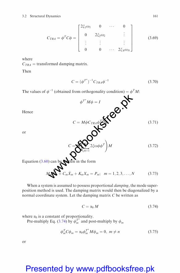
CTRA ¼ fTCf ¼
2x1o1 0 � � � 0
0 2x2o2...
..
. ... ..
.
0 0 � � � 2xNoN
2666664
3777775
(3:69)
whereCTRA ¼ transformed damping matrix.
Then
C ¼ ðfT 00 Þ�1CTRAf�1 (3:70)
The values of f�1 (obtained from orthogonality condition) ¼ fTM:
fT 00Mf ¼ I
Hence
C ¼MfCTRAfT 00M (3:71)
or
C ¼MXNm¼1
2xoffT
!M (3:72)
Equation (3.60) can be written in the form
Mm€Xm þ Cm
_Xm þ KmXm ¼ Pm; m ¼ 1; 2; 3; . . . ;N (3:73)
When a system is assumed to possess proportional damping, the mode super-position method is used. The damping matrix would then be diagonalized by anormal coordinate system. Let the damping matrix C be written as
C ¼ a0 M (3:74)
where a0 is a constant of proportionality.Pre-multiply Eq. (3.74) by fT 00
m and post-multiply by fm
fTmCfm ¼ a0f
T 00
m Mfm ¼ 0; m 6¼ n (3:75)
or
3.2 Structural Dynamics 161
www.pdfbo
oksfr
ee.pk
Presented by www.pdfbooksfree.pk
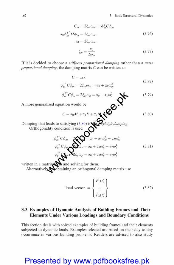
Cm ¼ 2xmom ¼ fTmCfm
a0fT 00
m Mfm ¼ 2xmom
a0 ¼ 2xmom
(3:76)
xm ¼a02om
(3:77)
If it is decided to choose a stiffness proportional damping rather than a massproportional damping, the damping matrix C can be written as
C ¼ a1k
fT 00
m Cfm ¼ 2xmom ¼ a0 þ a1o2m
(3:78)
fT 00
m Cfn ¼ 2xmon ¼ a0 þ a1o2n (3:79)
A more generalized equation would be
C ¼ a0Mþ a1Kþ a2M�1KM (3:80)
Damping that leads to satisfying (3.80) is the Rayleigh damping.Orthogonality condition is used
fT 00
m Cfm ¼ 2xmom ¼ a0 þ a1o2m þ a2o4
m
fT 00
m Cfn ¼ 2xnon ¼ a0 þ a1o2n þ a2o4
n
fT 00
p Cfp ¼ 2xpop ¼ a0 þ a1o2p þ a2o4
p
(3:81)
written in a matrix form and solving for them.Alternatively for obtaining an orthogonal damping matrix use
load vector ¼
P1ðtÞ...
PnðtÞ
8>><>>:
9>>=>>;
(3:82)
3.3 Examples of Dynamic Analysis of Building Frames and Their
Elements Under Various Loadings and Boundary Conditions
This section deals with solved examples of building frames and their elementssubjected to dynamic loads. Examples selected are based on their day-to-dayoccurrence in various building problems. Readers are advised to also study
162 3 Basic Structural Dynamics
www.pdfbo
oksfr
ee.pk
Presented by www.pdfbooksfree.pk
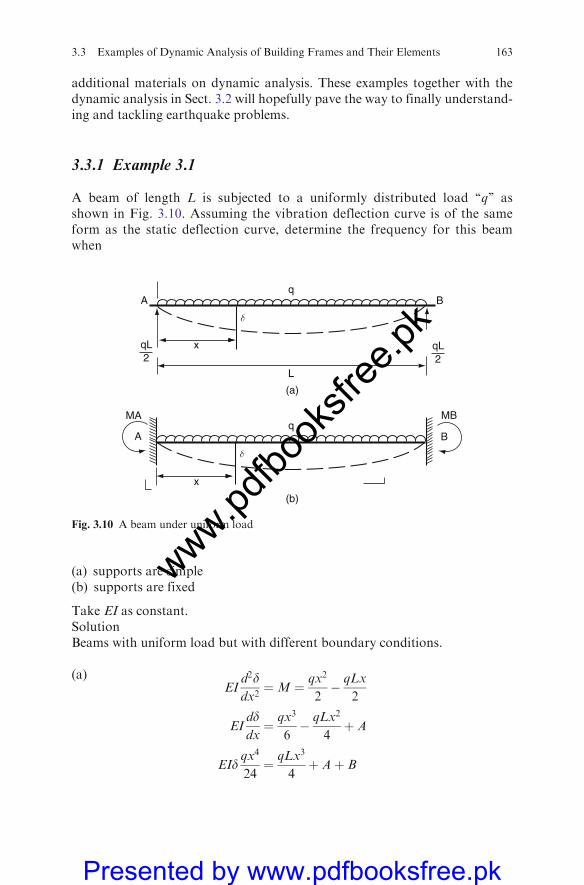
additional materials on dynamic analysis. These examples together with thedynamic analysis in Sect. 3.2 will hopefully pave the way to finally understand-ing and tackling earthquake problems.
3.3.1 Example 3.1
A beam of length L is subjected to a uniformly distributed load ‘‘q’’ asshown in Fig. 3.10. Assuming the vibration deflection curve is of the sameform as the static deflection curve, determine the frequency for this beamwhen
(a) supports are simple(b) supports are fixed
Take EI as constant.SolutionBeams with uniform load but with different boundary conditions.
(a)EI
d2ddx2¼M ¼ qx2
2� qLx
2
EIdddx¼ qx3
6� qLx2
4þ A
EIdqx4
24¼ qLx3
4þ Aþ B
(b)
(a)
A
L
x
qB
δ
qL2
qL2
MA
A
x
qB
MB
δ
Fig. 3.10 A beam under uniform load
3.3 Examples of Dynamic Analysis of Building Frames and Their Elements 163
www.pdfbo
oksfr
ee.pk
Presented by www.pdfbooksfree.pk

when the boundary conditions are
x ¼ 0 d ¼ 0 B ¼ 0
x ¼ L d ¼ 0 A ¼ qL3
24
EId ¼ 0 ¼ qL4
24� qL4
12þ AL
d ¼ q
24EIðx4 � 2Lx3 þ L3xÞ
Z L
0
ddx ¼ qL5
120EIZ L
0
d2dx ¼ 31
360L9 q
24EI
� �2
f ¼ 1
2p
ffiffiffiffiffiffiffiffiffiffiffiffiffiffiffiffiffiffiffiffiffiffiffiffiffiffiffiffiffiffiffiffiffiffiffiffiffiffiffiffiffiffiffiffiffiffiffiffiffiffiffiffiffiffiffiffiffigqL5
120EI
630
31L9
24EI
q
� �2( )vuut
¼ 1:572
ffiffiffiffiffiffiffiffiffiffiffiffiffiffiffiffiffiffiffiffiEIg
qL4ðHzÞ
s
(b)EI
d2ddx2¼M ¼MA þ
qx2
2� qL
2x
EIdddx¼MAxþ
qx3
6� qL
x2
4þ A
EId ¼ 1
2MAx
2 þ qx4
24� qLx3
12þ Axþ B
Boundary conditions:
x ¼ 0dddx¼ 0 A ¼ 0 B ¼ 0 d ¼ 0
x ¼ Ldddx¼ 0
EIdddx¼MALþ
qL3
6� qLx2
4þ 0
0 ¼MALþqL3
6� qL3
4or MA ¼
qL3
12
d ¼ q
24EI½L2x2 þ x4 � 2Lx3�
164 3 Basic Structural Dynamics
www.pdfbo
oksfr
ee.pk
Presented by www.pdfbooksfree.pk
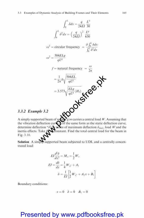
Z L
0
ddx ¼ q
24EI
L3
30Z L
0
d2dx ¼� q
24EI
�2 Lq
630
o2 ¼ circular frequency ¼dR L0 ddxR L
0 d2dx
o2 ¼ 504ELg
qL4
f ¼ natural frequency ¼ o2p
¼ 1
2pg
ffiffiffiffiffiffiffiffiffiffiffiffiffiffi504EL
qL4
s
¼ 3:573
ffiffiffiffiffiffiffiffiffiffiffiffiffiffiffiffiffiffiffiffiELg
qL4ðH2Þ
s
3.3.2 Example 3.2
A simply supported beam of weight q/m carries a central loadW.Assuming thatthe vibration deflection curve is of the same form as the static deflection curve,determine deflection ‘‘d’’ in terms of maximum deflection dmax, load W and theinertia effects. Take EI as constant. Find the total central load for the beam inFig. 3.10.
Solution A simply supported beam subjected to UDL and a centrally concen-trated load:
EId2ddx2¼Mx ¼
1
2Wx
EI ¼ dddx¼ 1
4Wx2 þ A1
d ¼ 1
EI
1
2Wx3 þ A1xþ B1
�
Boundary conditions:
x ¼ 0 d ¼ 0 B1 ¼ 0
3.3 Examples of Dynamic Analysis of Building Frames and Their Elements 165
www.pdfbo
oksfr
ee.pk
Presented by www.pdfbooksfree.pk
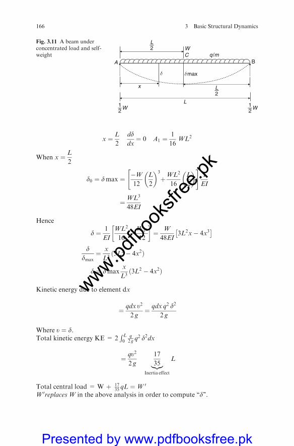
x ¼ L
2
dddx¼ 0 A1 ¼
1
16WL2
When x ¼ L
2
d0 ¼ dmax ¼ �W12
L
2
� �3
þWL2
16
L
2
� �" #1
EI
¼WL3
48EI
Hence
d ¼ 1
EI
WL2
16�Wx3
12
�¼ W
48EI3L2x� 4x3� �
ddmax
¼ x
L3ð3L2 � 4x2Þ
d ¼ dmaxx
L3ð3L2 � 4x2Þ
Kinetic energy due to element dx
¼ qdx u2
2 g¼ qdx q2 d2
2 g
Where u ¼ d.Total kinetic energy KE = 2
R L0
q2 g q
2 d2dx
¼ qu2
2 g
17
35|{z}Inertia effect
L
Total central load = W þ 1735 qL ¼W 0
W 0replaces W in the above analysis in order to compute ‘‘d’’.
A
WC
B
δ
x
WL
q /m
δmax
21
2L
2L
W21
Fig. 3.11 A beam underconcentrated load and self-weight
166 3 Basic Structural Dynamics
www.pdfbo
oksfr
ee.pk
Presented by www.pdfbooksfree.pk
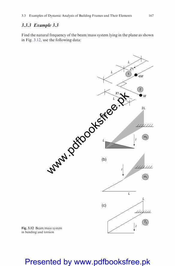
3.3.3 Example 3.3
Find the natural frequency of the beam/mass system lying in the plane as shown
in Fig. 3.12, use the following data:
L
L
Z1
X1
L
1
2
M
4M
2L
m2L I
m1
I
L
L
IT2
(a)
(b)
(c)
Fig. 3.12 Beam/mass systemin bending and torsion
3.3 Examples of Dynamic Analysis of Building Frames and Their Elements 167
www.pdfbo
oksfr
ee.pk
Presented by www.pdfbooksfree.pk
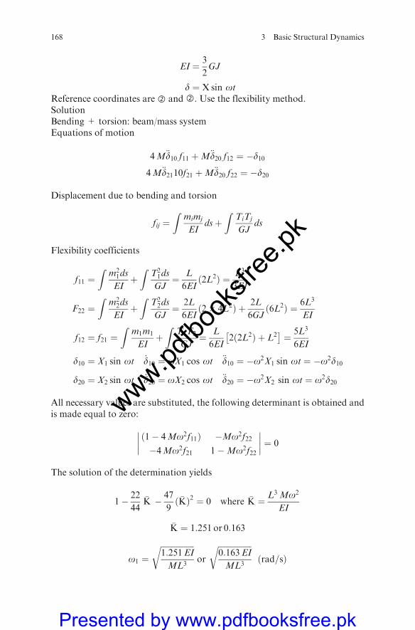
EI ¼ 3
2GJ
d ¼ Xsin otReference coordinates areffl andffl. Use the flexibility method.SolutionBending + torsion: beam/mass systemEquations of motion
4M€d10 f11 þM€d20 f12 ¼ �d104M€d2110f21 þM€d20 f22 ¼ �d20
Displacement due to bending and torsion
fij ¼Z
mimj
EIdsþ
ZTiTj
GJds
Flexibility coefficients
f11 ¼Z
m21ds
EIþZ
T21ds
GJ¼ L
6EIð2L2Þ ¼ L3
3EI
F22 ¼Z
m22ds
EIþZ
T22ds
GJ¼ 2L
6EIð2� 4L2Þ þ 2L
6GJð6L2Þ ¼ 6L3
EI
f12 ¼ f21 ¼Z
m1m1
EIþZ
T1T2
GJ¼ L
6EI2ð2L2Þ þ L2� �
¼ 5L3
6EI
d10 ¼ X1 sin ot _d10 ¼ oX1 cos ot €d10 ¼ �o2X1 sin ot ¼ �o2d10
d20 ¼ X2 sin ot _d20 ¼ oX2 cos ot €d20 ¼ �o2X2 sin ot ¼ o2d20
All necessary values are substituted, the following determinant is obtained andis made equal to zero:
ð1� 4Mo2f11Þ �Mo2f22
�4Mo2f21 1�Mo2f22
�������� ¼ 0
The solution of the determination yields
1� 22
44�K � 47
9ð �KÞ2 ¼ 0 where �K ¼ L3 Mo2
EI
�K ¼ 1:251 or 0:163
o1 ¼ffiffiffiffiffiffiffiffiffiffiffiffiffiffiffiffiffi1:251EI
ML3
ror
ffiffiffiffiffiffiffiffiffiffiffiffiffiffiffiffiffi0:163EI
ML3
rðrad=sÞ
168 3 Basic Structural Dynamics
www.pdfbo
oksfr
ee.pk
Presented by www.pdfbooksfree.pk
f ðlowestÞ ¼ 1
2p
ffiffiffiffiffiffiffiffiffiffiffiffiffiffiffiffiffiffiffiffiffiffi0:163EI
ML3
�s
3.3.4 Example 3.4
A frame lying in a plane with a distributed mass of 1,500 kg/m is shown inFig. 3.13. Using the flexibility method or otherwise, determine the naturalfrequency ‘‘f’’ for this frame. Use the following data:
E = 14 � 106 kN/m2
I = 2,600 � 10�6 m4
G = 6.4 � 106 kN/m2
J = 1,800 � 10�6 m4
L = 4md = X sin o tEI = 14 � 106 kN/m2 � 2600 � 10�6
GJ = 6.4 � 106 kN/m2 � 1800 � 10�6
Use the direct integration process.SolutionA bent in-plane subject to a distributed mass. Different coordinate systems x
and y apply:
C
L = 4m
L = 4m
x
y
B
A
1500 kg/m
Fig. 3.13 A frame in-plane
3.3 Examples of Dynamic Analysis of Building Frames and Their Elements 169
www.pdfbo
oksfr
ee.pk
Presented by www.pdfbooksfree.pk

fij ¼Z
mimj
EIdsþ
ZTiTj
GJ
d ¼ �o2X sin ot
Flexibility parameters Limits
m1 = 1 � L 0 � y � L
m1 = 1 � L 0 � x � L
m2 = 1 � L 0 � y � L
m2 = 1 � L 0 � x � L
T1 ¼ 12L 0 � y � L
T1 ¼ 12L 0 � x � L
T2 ¼ 12L 0 � y � L
T2 ¼ 12L 0 � x � L
Flexibility coefficients
f11 ¼ 2
Z L
0
L2
EIdLþ 2
Z L
0
L2
4GJ2dL ¼ 2L3
3EIþ L3
6GJ¼ 0:0021
EI
f22 ¼ 2
Z L
0
LdL
EIþ 2
Z L
0
L2
4GJdL ¼ 0:0014
EI
f12 ¼ f21 ¼2
EI
Z L
0
L2dLþ 2
GJ
Z L
0
L2 dL ¼ 0:0021
EI
Equations of motion:
M1€d10 f11 þM2
€d20 f12 ¼ �d10
M1€d10 f12 þM2
€d20 f22 ¼ �d20
Substituting respective values, the following relations are established:
0:1029w2 � 1� �
0:062w2
0:1029w2 0:041w2 � 1� �
" #X1X2
n o¼ 0
0
Solving the determinant of the matrix X1 6¼ 0; X2 6¼ 0 and making K ¼ o2
�K ¼ �0:1439� 0:1718
0:0044
o ¼ 2:51ðthe lowest rad =sÞ
F ¼ o2p¼ 0:4HZ
170 3 Basic Structural Dynamics
www.pdfbo
oksfr
ee.pk
Presented by www.pdfbooksfree.pk
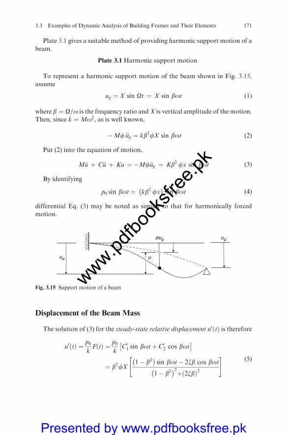
Plate 3.1 gives a suitable method of providing harmonic support motion of a
beam.
Plate 3.1 Harmonic support motion
To represent a harmonic support motion of the beam shown in Fig. 3.15,
assume
ug ¼ X sin Ot ¼ X sin bot (1)
where b ¼ O=o is the frequency ratio andX is vertical amplitude of the motion.
Then, since k ¼Mo2, as is well known,
�Mf €ug ¼ kb2fX sin bot (2)
Put (2) into the equation of motion,
M€u þ C€u þ Ku ¼ �Mf€ug ¼ Kb2 fx sin bot (3)
By identifying
p0 sin bot ¼ kb2 fx� �
sin bot (4)
differential Eq. (3) may be noted as similar to that for harmonically forced
motion.
Displacement of the Beam Mass
The solution of (3) for the steady-state relative displacement u0 tð Þ is therefore
u0 tð Þ ¼ p0
kF tð Þ ¼ p0
kC01 sin botþ C02 cos bot� �
¼ b2fX1� b2� �
sin bot� 2xb cos bot
1� b2� �2þ 2xbð Þ2
" #(5)
ugøug
uua
Fig. 3.15 Support motion of a beam
3.3 Examples of Dynamic Analysis of Building Frames and Their Elements 171
www.pdfbo
oksfr
ee.pk
Presented by www.pdfbooksfree.pk
from which the maximum value may be written as
u0max ¼p0kFmax ¼ b2fXFmax (6)
where
Fmax ¼1ffiffiffiffiffiffiffiffiffiffiffiffiffiffiffiffiffiffiffiffiffiffiffiffiffiffiffiffiffiffiffiffiffiffiffi
i� b2� �2þ 2xbð Þ2
q (7)
Consequently, the steady-state absolute displacement ua tð Þ of the beam mass isgiven by
ua tð Þ ¼ fug tð Þ þ u tð Þ ¼ fx1� b2 þ 4x2b2� �
sin bot� 2xb3 cos bot
1� b2� �2þ 2xbð Þ2
(8)
and its maximum value is found (after manipulation) to be
umax ¼ fxFmax
ffiffiffiffiffiffiffiffiffiffiffiffiffiffiffiffiffiffiffiffiffiffi1þ 2xbð Þ2
q(9)
For most practical values of x and b the square root factor is almost equal tounity.
Equivalent Static Load on the Beam
From the equation of motion of the beam mass, the equivalent static load is
Pequiv ¼M€ua (10)
Pequiv ¼ Kuþ C _u ¼ K uþ 2xo
_u
�(11)
Through the use of (8), (10) gives the following result:
Pequiv ¼ b2kua tð Þ ¼ b2 kfX1� b2 þ 4x2b2� �
sin bot� 2xb2 cos bot
1� b2� �2þ 2xbð Þ2
" #(12)
using (9), the maximum value can be achieved as
Pequivmax ¼ b2 kf Fmax
ffiffiffiffiffiffiffiffiffiffiffiffiffiffiffiffiffiffiffiffiffiffi1þ 2xbð Þ2
q �(13)
3.3.5 Example 3.5
A single-bay two-storey frame is shown in Fig. 3.14. Derive equations ofmotion.
For displacements x1 and x2, the tensions in the springs are
P1 ¼ k1x1 and P2 ¼ k2 x2 � x1ð Þ
172 3 Basic Structural Dynamics
www.pdfbo
oksfr
ee.pk
Presented by www.pdfbooksfree.pk
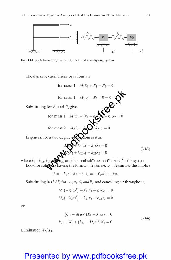
The dynamic equilibrium equations are
for mass 1 M1€x1 þ P1 � P2 ¼ 0
for mass 1 M2€x2 þ P2 � 0 ¼ 0
Substituting for P1 and P2 gives
for mass 1 M1€x1 þ ðk1 þ k2Þ x1 � k2 x2 ¼ 0
for mass 2 M2€x2 � k2x1 þ k2x2 ¼ 0
In general for a two-degree-of-freedom system
M1€x1 þ k11x1 þ k12x2 ¼ 0
M2€x2 þ k12x1 þ k22x2 ¼ 0(3:83)
where k11, k12, k21 and k22 are the usual stiffness coefficients for the system.Look for solutions having the form x1¼X1 sinot, x2¼;X2 sinot; this implies
€x ¼ �X1o2 sin ot; €x2 ¼ �X2o2 sin ot:
Substituting in (3.83) for x1; x2; €x1 and €x2 and cancelling ot throughout,
M1 �X1o2� �
þ k11x1 þ k12x2 ¼ 0
M2 �X2o2� �
þ k21x1 þ k22x2 ¼ 0
or
k11 �M1o2� �
X1 þ k12x2 ¼ 0
k21 þ X1 þ k22 �M2o2� �
X2 ¼ 0(3:84)
Elimination X2=X1,
1
2
M1 M2
x1 x2
k2k1
Fig. 3.14 (a) A two-storey frame. (b) Idealized mass/spring system
3.3 Examples of Dynamic Analysis of Building Frames and Their Elements 173
www.pdfbo
oksfr
ee.pk
Presented by www.pdfbooksfree.pk
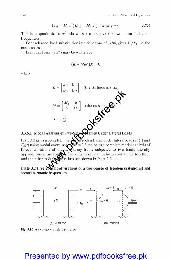
k11 �M1o2� �
k22 �M2o2� �
� k12k21 ¼ 0 (3:85)
This is a quadratic in o2 whose two roots give the two natural circularfrequencies.
For each root, back substitution into either one of (3.84) givesX2=X1; i.e. themode shape.
In matrix form, (3.84) may be written as
K�Mo2� �
X ¼ 0
where
K ¼k11 k12
k21 k22
�ðthe stiffness matrixÞ
M ¼M1 0
0 M2
�ðthe mass matrixÞ
X ¼ X1
X2
h i
3.3.5.1 Modal Analysis of Two-Storey Frames Under Lateral Loads
Plate 3.2 gives a complete analysis of such a frame under lateral loads F1 tð Þ andF2 tð Þ using modal coordinates. Plate 3.3 indicates a complete modal analysis offorced vibrations of the two-storey frame subjected to two loads laterallyapplied, one is an applied load of a triangular pulse placed at the top floorand the other is F tð Þ. The values are shown in Plate 3.3.
Plate 3.2 Free undamped virations of a two degree of freedom system-first and
second harmonic frequencies
x2
x1
EI
EI
EI
EI
L
L
k
k
x1 = 1 k
2k
x1 = 0
x2 = 1x2 = 0
M
2M
(a) A frame (b) modes
Fig. 3.16 A two-story single-bay frame
174 3 Basic Structural Dynamics
www.pdfbo
oksfr
ee.pk
Presented by www.pdfbooksfree.pk

Equations of Motion
M€xþ kx ¼ 0
M 0
0 2M
" #€x1
€x2
" #þ
k �k
�k 2 k
" #x1
x2
" #¼
0
0
" #(1)
Trial Solution
x tð Þ ¼ x A sin otþ B cos otð Þ
x1 tð Þ
x2 tð Þ
" #x1
x2
" #A sin otþ B cos otð Þ
(2)
The Eigenvalue Problem
By substituting (2) into (1), we obtain the necessary conditions for (2) to be asolution
k� o2 M� �
x ¼ 0 (3)
1� bð Þ �1�1 2 1� bð Þ
�x1
x2
�¼
0
0
�b ¼ o2 M=k (4)
Using nontrivial solutions to (3), i.e. solutions where the eigenvectors f 6¼ 0,
k� o2 M�� �� ¼ 0 (5)
Equation (5) if the frequency equation from which the eigenvalues o2 can beobtained
2 1� bð Þ2�1 ¼ 0 or 2b2 � 4bþ 1 ¼ 0 ! b� 1
2
ffiffiffi2p
(6)
b1¼ 0:2929; b2 ¼ 1:7071 (7)
Natural Circular Frequencies and Natural Periods
First harmonic
o1
ffiffiffiffiffiffiffiffiffiffiffiffiffiffiffib1k=M
p; T1 ¼
2po1
(8)
Second harmonic
o2
ffiffiffiffiffiffiffiffiffiffiffiffiffiffiffib2k=M
p; T2 ¼
2po2
(9)
3.3 Examples of Dynamic Analysis of Building Frames and Their Elements 175
www.pdfbo
oksfr
ee.pk
Presented by www.pdfbooksfree.pk
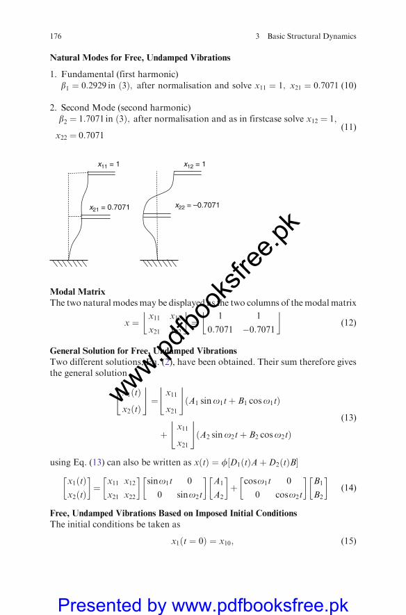
Natural Modes for Free, Undamped Vibrations
1. Fundamental (first harmonic)b1 ¼ 0:2929 in ð3Þ; after normalisation and solve x11 ¼ 1; x21 ¼ 0:7071 (10)
2. Second Mode (second harmonic)b2 ¼ 1:7071 in ð3Þ; after normalisation and as in firstcase solve x12 ¼ 1;
x22 ¼ 0:7071(11)
x11 = 1 x12 = 1
x22 = –0.7071x21 = 0.7071
Modal Matrix
The two natural modes may be displayed as the two columns of themodal matrix
x ¼x11 x12
x21 x22
� �¼
1 1
0:7071 �0:7071
� �(12)
General Solution for Free, Undamped Vibrations
Two different solutions, Eq. (2), have been obtained. Their sum therefore givesthe general solution
x1ðtÞ
x2ðtÞ
$ %¼
x11
x21
$ %ðA1 sino1tþ B1 coso1tÞ
þx11
x21
$ %ðA2 sino2tþ B2 coso2tÞ
(13)
using Eq. (13) can also be written as xðtÞ ¼ f½D1ðtÞAþD2ðtÞB�
x1ðtÞx2ðtÞ
�¼
x11 x12
x21 x22
�sino1t 0
0 sino2t
�A1
A2
�þ
coso1t 0
0 coso2t
�B1
B2
�(14)
Free, Undamped Vibrations Based on Imposed Initial Conditions
The initial conditions be taken as
x1ðt ¼ 0Þ ¼ x10; (15)
176 3 Basic Structural Dynamics
www.pdfbo
oksfr
ee.pk
Presented by www.pdfbooksfree.pk
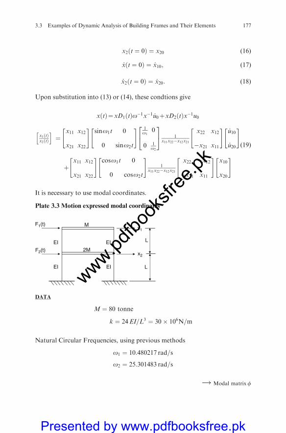
x2ðt ¼ 0Þ ¼ x20 (16)
_xðt ¼ 0Þ ¼ _x10; (17)
_x2ðt ¼ 0Þ ¼ _x20: (18)
Upon substitution into (13) or (14), these condtions give
xðtÞ¼xD1ðtÞo�1x�1 _u0þxD2ðtÞx�1u0
x1ðtÞx2ðtÞ
h i¼
x11 x12
x21 x22
" #sino1t 0
0 sino2t
" # 1o1
0
0 1o2
24
35 1
x11x22�x12x21
x22 x12
�x21 x11
" #_u10
_u20
" #
þx11 x12
x21 x22
" #coso1t 0
0 coso2t
" #1
x11x22�x12x21
x22 �x12
�x21 x11
" #x10
x20
" #(19)
It is necessary to use modal coordinates.
Plate 3.3 Motion expressed modal coordinates
F2(t)
x1
EI
EI
EI
EI
L
L
M
2M
F1(t)
x2
DATA
M ¼ 80 tonne
k ¼ 24EI=L3 ¼ 30� 106N=m
Natural Circular Frequencies, using previous methods
o1 ¼ 10:480217 rad=s
o2 ¼ 25:301483 rad=s
! Modal matrixf
3.3 Examples of Dynamic Analysis of Building Frames and Their Elements 177
www.pdfbo
oksfr
ee.pk
Presented by www.pdfbooksfree.pk
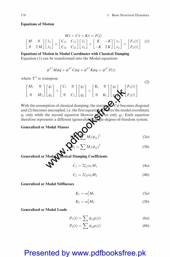
Equations of Motion
M _xþ C _xþ K _x ¼ FðtÞM 0
0 2M
�€x1
€x2
�þ
C11 C12
C21 C22
�_x1
_x2
�þ
K �K�K 2K
�x1
x2
�¼
F1ðtÞF2ðtÞ
�(1)
Equations of Motion in Modal Coordinates with Classical Damping
Equation (1) can be transformed into the Modal equations
fT 00Mf€qþ fT 00Cf _qþ fT 00Kfq ¼ fT 00FðtÞ
where T 00 is transpose
M1 0
0 M2
" #€q1
€q2
" #þ
C1 0
0 C2
" #_q1
_q2
" #þ
K1 0
0 K1
" #q1
q2
" #¼
F1ðtÞ
F2ðtÞ
" # (2)
With the assumption of classical damping, the matrix fT 00Cf becomes diagonaland (2) becomes uncoupled, i.e. the first equation involves themodal coordinateq1 only while the second equation likewise involves only q2. Each equationtherefore represents a different (generalized) single-degree-of-freedom system.
Generalized or Modal Masses
M1 ¼X
Miðfi1Þ2 (3a)
M2 ¼X
Miðfi2Þ2 (3b)
Generalized or Modal Classical Damping Coefficients
C1 ¼ 2x1o1M1 (4a)
C2 ¼ 2x2o2M2 (4b)
Generalized or Modal Stiffnesses
K1 ¼ o21M1 (5a)
K2 ¼ o22M2 (5b)
Generalized or Modal Loads
P1ðtÞ ¼X
fi1piðtÞ (6a)
P2ðtÞ ¼X
fi2piðtÞ (6b)
178 3 Basic Structural Dynamics
www.pdfbo
oksfr
ee.pk
Presented by www.pdfbooksfree.pk
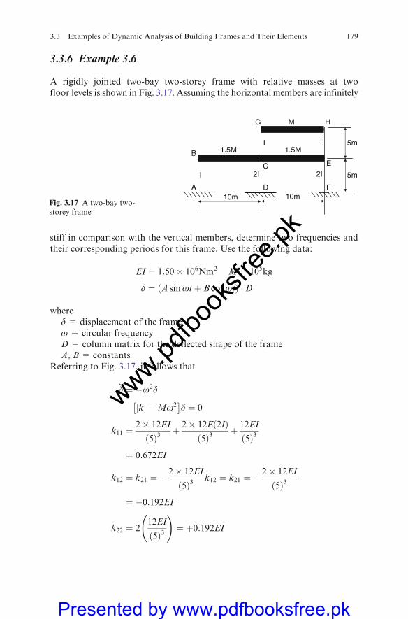
3.3.6 Example 3.6
A rigidly jointed two-bay two-storey frame with relative masses at twofloor levels is shown in Fig. 3.17. Assuming the horizontal members are infinitely
stiff in comparison with the vertical members, determine two frequencies andtheir corresponding periods for this frame. Use the following data:
EI ¼ 1:50� 106Nm2 M ¼ 105kg
d ¼ ðA sinotþ B cosotÞ �D
whered = displacement of the frameo = circular frequencyD = column matrix for the deflected shape of the frameA, B = constants
Referring to Fig. 3.17, it follows that
€d ¼ �o2d
k½ � �Mo2� �
d ¼ 0
k11 ¼2� 12EI
ð5Þ3þ 2� 12Eð2IÞ
ð5Þ3þ 12EI
ð5Þ3
¼ 0:672EI
k12 ¼ k21 ¼ �2� 12EI
ð5Þ3k12 ¼ k21 ¼ �
2� 12EI
ð5Þ3
¼ �0:192EI
k22 ¼ 212EI
ð5Þ3
!¼ þ0:192EI
H
2I
I
I 5m
5m
M
1.5M
G
1.5M
10m 10m
2I
E
FD
C
B
A
I
Fig. 3.17 A two-bay two-storey frame
3.3 Examples of Dynamic Analysis of Building Frames and Their Elements 179
www.pdfbo
oksfr
ee.pk
Presented by www.pdfbooksfree.pk
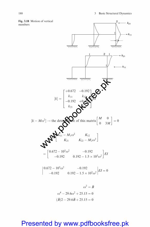
½k� ¼
þ0:672 �0:192k11 k12
�0:192 þ0:192k21 k22
26664
37775EI
½k�Mo2� ! the determinant of this matrixM 0
0 3M
�¼ 0
EIK11 �M1o2 K12
K21 K22 �M2o2
�
¼ 0:672� 105o2 �0:192�0:192 0:192� 1:5� 105o2
�EI
0:672� 105o2 �0:192�0:192 0:192� 1:5� 105o2
��������EI ¼ 0
o2 ¼ �B
o4 � 29:6o2 þ 25:15 ¼ 0
ð �BÞ2� 29:6 �Bþ 25:15 ¼ 0
k21
I
I
2
k11
k21
I
2
k11
II
Fig. 3.18 Motion of verticalmembers
180 3 Basic Structural Dynamics
www.pdfbo
oksfr
ee.pk
Presented by www.pdfbooksfree.pk
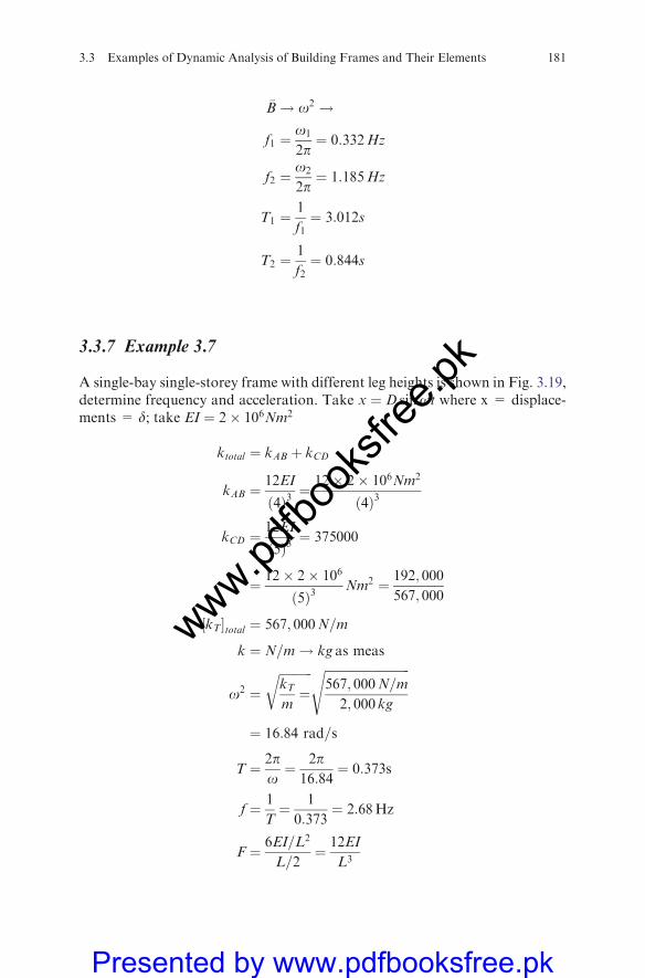
�B! o2 !
f1 ¼o1
2p¼ 0:332Hz
f2 ¼o2
2p¼ 1:185Hz
T1 ¼1
f1¼ 3:012s
T2 ¼1
f2¼ 0:844s
3.3.7 Example 3.7
A single-bay single-storey frame with different leg heights is shown in Fig. 3.19,determine frequency and acceleration. Take x ¼ D sinot where x = displace-ments = d; take EI ¼ 2� 106Nm2
ktotal ¼ kAB þ kCD
kAB ¼12EI
ð4Þ3¼ 12� 2� 106Nm2
ð4Þ3
kCD ¼12EI
ð5Þ3¼ 375000
¼ 12� 2� 106
ð5Þ3Nm2 ¼ 192; 000
567; 000
½kT�total ¼ 567; 000N=m
k ¼ N=m! kg as meas
o2 ¼ffiffiffiffiffiffiffiffiffiffiffikTm¼
r ffiffiffiffiffiffiffiffiffiffiffiffiffiffiffiffiffiffiffiffiffiffiffiffiffiffiffiffi567; 000N=m
2; 000 kg
s
¼ 16:84 rad=s
T ¼ 2po¼ 2p
16:84¼ 0:373s
f ¼ 1
T¼ 1
0:373¼ 2:68Hz
F ¼ 6EI=L2
L=2¼ 12EI
L3
3.3 Examples of Dynamic Analysis of Building Frames and Their Elements 181
www.pdfbo
oksfr
ee.pk
Presented by www.pdfbooksfree.pk
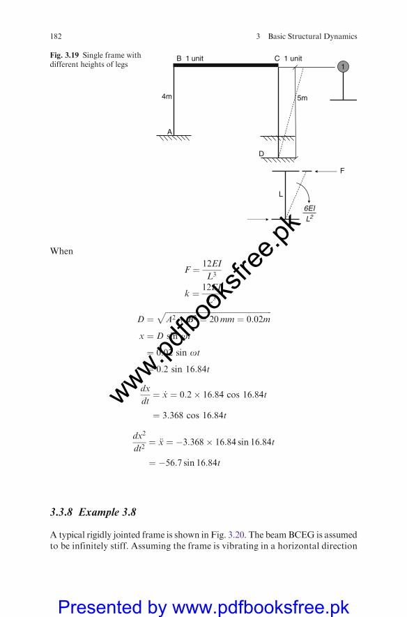
When
F ¼ 12EI
L3
k ¼ 12EI
L3
D ¼ffiffiffiffiffiffiffiffiffiffiffiffiffiffiffiffiffiffiffiffiffiffiffiffiffiffiffiffiffiffiffiffiffiffiffiffiffiffiffiffiffiffiffiffiffiffiffiffiffiffiffiffiffiffiffiA2 þ B2 ¼ 20mm ¼ 0:02m
px ¼ D sin ot
¼ 0:02 sin ot
¼ 0:2 sin 16:84t
dx
dt¼ _x ¼ 0:2� 16:84 cos 16:84t
¼ 3:368 cos 16:84t
dx2
dt2¼ €x ¼ �3:368� 16:84 sin 16:84t
¼ �56:7 sin 16:84t
3.3.8 Example 3.8
A typical rigidly jointed frame is shown in Fig. 3.20. The beamBCEG is assumedto be infinitely stiff. Assuming the frame is vibrating in a horizontal direction
1C 1 unitB 1 unit
4m
A
D
5m
6EIL2
F
L
Fig. 3.19 Single frame withdifferent heights of legs
182 3 Basic Structural Dynamics
www.pdfbo
oksfr
ee.pk
Presented by www.pdfbooksfree.pk
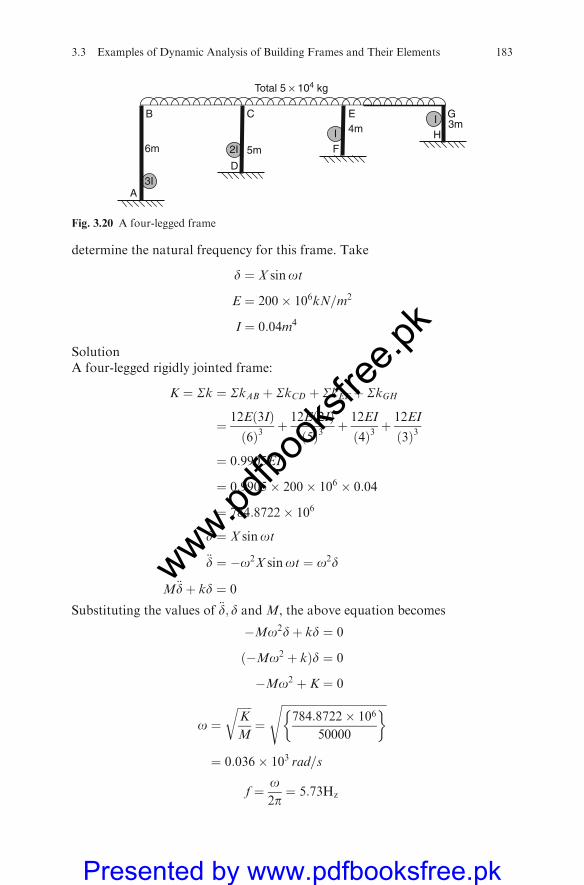
determine the natural frequency for this frame. Take
d ¼ X sinot
E ¼ 200� 106kN=m2
I ¼ 0:04m4
SolutionA four-legged rigidly jointed frame:
K ¼ Sk ¼ SkAB þ SkCD þ SkEF þ SkGH
¼ 12Eð3IÞð6Þ3
þ 12Eð2IÞð5Þ3
þ 12EI
ð4Þ3þ 12EI
ð3Þ3
¼ 0:9905EI
¼ 0:9905� 200� 106 � 0:04
¼ 784:8722� 106
d ¼ X sinot
€d ¼ �o2X sinot ¼ o2d
M€dþ kd ¼ 0
Substituting the values of €d; d and M, the above equation becomes
�Mo2dþ kd ¼ 0
ð�Mo2 þ kÞd ¼ 0
�Mo2 þ K ¼ 0
o ¼ffiffiffiffiffiK
M
r¼
ffiffiffiffiffiffiffiffiffiffiffiffiffiffiffiffiffiffiffiffiffiffiffiffiffiffiffiffiffiffiffiffiffiffiffiffiffiffi784:8722� 106
50000
� �s
¼ 0:036� 103 rad=s
f ¼ o2p¼ 5:73Hz
II
3I
2I
C
H
E
Total 5 × 10⁴ kg
3mG
F
4m
D
5m
A
B
6m
Fig. 3.20 A four-legged frame
3.3 Examples of Dynamic Analysis of Building Frames and Their Elements 183
www.pdfbo
oksfr
ee.pk
Presented by www.pdfbooksfree.pk
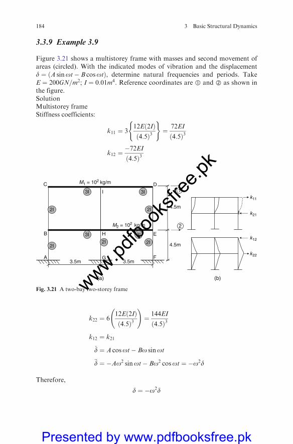
3.3.9 Example 3.9
Figure 3.21 shows a multistorey frame with masses and second movement ofareas (circled). With the indicated modes of vibration and the displacementd ¼ ðA sinot� B cosotÞ, determine natural frequencies and periods. TakeE ¼ 200GN=m2; I ¼ 0:01m4. Reference coordinates are ffi and ffl as shown inthe figure.SolutionMultistorey frameStiffness coefficients:
k11 ¼ 312Eð2IÞð4:5Þ3
( )¼ 72EI
ð4:5Þ3
k12 ¼�72EIð4:5Þ3
k22 ¼ 612Eð2IÞð4:5Þ3
!¼ 144EI
ð4:5Þ3
k12 ¼ k21
_d ¼ A cosot� Bo sinot
€d ¼ �Ao2 sinot� Bo2 cosot ¼ �o2d
Therefore,
d ¼ �o2d
2I
2I
3I
3I 3I2I 2I
G
2I
3Ik11
I
3.5m
k21
k12
k22
3.5m
4.5m
4.5m
M1 = 102 kg/m
M2 = 102 kg/m
1
2
E
F
I
A
(a)
C
B H
D
(b)
Fig. 3.21 A two-bay two-storey frame
184 3 Basic Structural Dynamics
www.pdfbo
oksfr
ee.pk
Presented by www.pdfbooksfree.pk
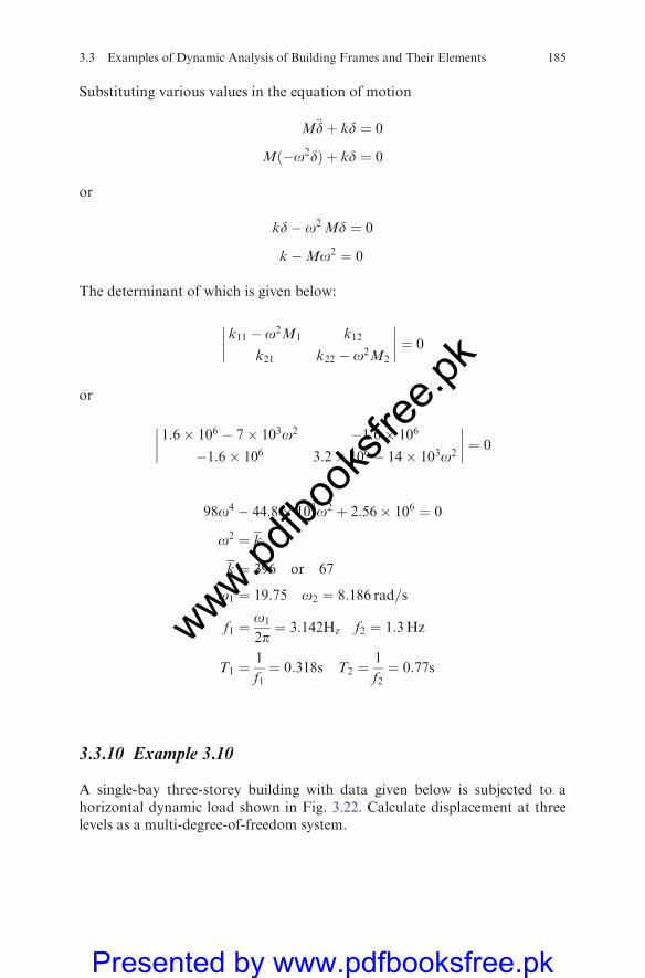
Substituting various values in the equation of motion
M€dþ kd ¼ 0
Mð�o2dÞ þ kd ¼ 0
or
kd� o2 Md ¼ 0
k�Mo2 ¼ 0
The determinant of which is given below:
k11 � o2M1 k12
k21 k22 � o2M2
�������� ¼ 0
or
1:6� 106 � 7� 103o2 �1:6� 106
�1:6� 106 3:2� 106 � 14� 103o2
�������� ¼ 0
98o4 � 44:8� 103o2 þ 2:56� 106 ¼ 0
o2 ¼ k
k ¼ 396 or 67
o1 ¼ 19:75 o2 ¼ 8:186 rad=s
f1 ¼o1
2p¼ 3:142Hz f2 ¼ 1:3Hz
T1 ¼1
f1¼ 0:318s T2 ¼
1
f2¼ 0:77s
3.3.10 Example 3.10
A single-bay three-storey building with data given below is subjected to ahorizontal dynamic load shown in Fig. 3.22. Calculate displacement at threelevels as a multi-degree-of-freedom system.
3.3 Examples of Dynamic Analysis of Building Frames and Their Elements 185
www.pdfbo
oksfr
ee.pk
Presented by www.pdfbooksfree.pk
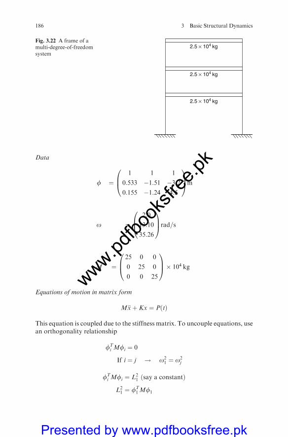
Data
f ¼1 1 1
0:533 �1:51 �3:20:155 �1:24 4:5
0B@
1CAm
o ¼2:0
13:10
35:26
0B@
1CArad=s
M ¼25 0 0
0 25 0
0 0 25
0B@
1CA� 104 kg
Equations of motion in matrix form
M€xþ Kx ¼ PðtÞ
This equation is coupled due to the stiffness matrix. To uncouple equations, usean orthogonality relationship
fTi Mfi ¼ 0
If i ¼ j ! o21 ¼ o2
j
fTi Mfi ¼ L2
1 ðsay a constantÞ
L21 ¼ fT
1Mf1
2.5 × 10⁴ kg
2.5 × 10⁴ kg
2.5 × 10⁴ kg
Fig. 3.22 A frame of amulti-degree-of-freedomsystem
186 3 Basic Structural Dynamics
www.pdfbo
oksfr
ee.pk
Presented by www.pdfbooksfree.pk

¼ ð1; 0:533; 0:155Þ25; 000 0 0
0 25; 000 0
0 0 25; 000
0B@
1CA
1
0:533
0:155
0B@
1CA
¼ð25; 000; 13; 325; 38; 75Þ1
0:533
0:155
0B@
1CA
¼ 32; 702:35) L1 ¼ 180:84 kg1=2m
L22 ¼ fT
2Mf2
¼ ð1 � 1:51� 1:24Þ25; 000 0 0
0 25; 000 0
0 0 25; 000
0B@
1CA
1
�1:51�1:24
0B@
1CA
¼ ð25; 000 � 37; 250 � 31; 000Þ1
�1:51�1:24
0B@
1CA
¼ 120; 442:5 ) L2 ¼ 347:048kg1=2m
L23 � fT
3Mf3
¼ ð1:0 � 3:2; 4:5Þ25; 000 0 0
0 25; 000 0
0 0 25; 000
0B@
1CA
1:0
�3:24:5
0B@
1CA
¼ ð25; 000 � 80; 000; 112; 500Þ1:0
�3:24:5
0B@
1CA
¼ 787; 250) L3 ¼ 897:27kg1=2m
The following can now be written:
zi ¼fi
Li
which gives
zTi Mzi ¼fTi M fi
L21
¼ 1
and
zTi M zj ¼ 0
3.3 Examples of Dynamic Analysis of Building Frames and Their Elements 187
www.pdfbo
oksfr
ee.pk
Presented by www.pdfbooksfree.pk
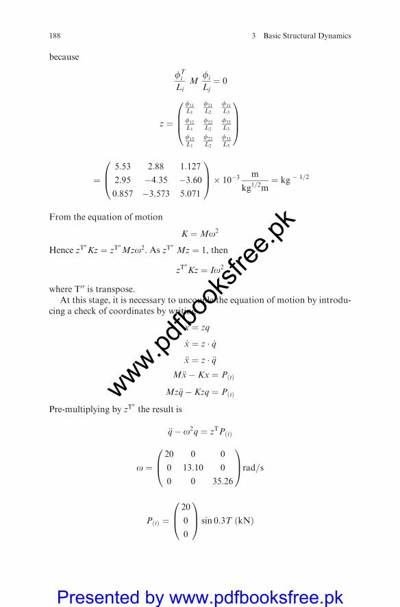
because
fTi
LiM
fi
Lj¼ 0
z ¼
f11
L1
f21
L2
f31
L3
f12
L1
f22
L2
f32
L3
f13
L1
f23
L2
f33
L3
0BB@
1CCA
¼5:53 2:88 1:127
2:95 �4:35 �3:600:857 �3:573 5:071
0B@
1CA� 10�3
m
kg1=2m¼ kg � 1=2
From the equation of motion
K ¼Mo2
Hence zT00Kz ¼ zT
00Mzo2. As zT
00Mz ¼ 1, then
zT00Kz ¼ Io2
where T00 is transpose.At this stage, it is necessary to uncouple the equation of motion by introdu-
cing a check of coordinates by writing
x ¼ zq
_x ¼ z � _q
€x ¼ z � €qM€x� Kx ¼ PðtÞ
Mz€q� Kzq ¼ PðtÞ
Pre-multiplying by zT00the result is
€q� o2q ¼ zTPðtÞ
o ¼20 0 0
0 13:10 0
0 0 35:26
0B@
1CArad=s
PðtÞ ¼20
0
0
0B@
1CA sin 0:3T ðkNÞ
188 3 Basic Structural Dynamics
www.pdfbo
oksfr
ee.pk
Presented by www.pdfbooksfree.pk
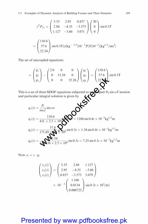
zTPðtÞ ¼5:53 2:95 0:857
2:88 �4:35 �3:5731:127 �3:60 5:071
0B@
1CA
20
0
0
0B@
1CA sin 0:3T
¼110:6
57:6
22:54
0B@
1CA sin 0:3Tðz½kg � 1=2�10� 3P½N�10�3Þ½kg1=2=ms2�
The set of uncoupled equations:
¼€q1
€q2
€q3
0B@
1CA�
2:0 0 0
0 13:10 0
0 0 35:26
0B@
1CA
q1
q2
q3
0B@
1CA ¼
110:6
57:6
22:54
0B@
1CA sin 0:3T
This is a set of three SDOF equations subjected to undamped P0 sinoTmotion
and particular integral solution is given by
q1ðtÞ ¼Pi
mo2i
sinot
q1ðtÞ ¼110:6
4:0:� 2:5� 104sin 0:3t ¼ 1106 sin 0:4t� 10�3kg1=2m
q2ðtÞ ¼57:6
171:69� 2:5� 104sin 0:3t ¼ 1:34 sin 0:4t� 10�5kg1=2m
q3ðtÞ ¼22:54
1243:36� 2:5� 104sin 0:3t ¼ 7:25 sin 0:3t� 10�7kg1=2m
Now xi ¼ z � qi
x1ðtÞx2ðtÞx3ðtÞ
0B@
1CA ¼
5:53 2:88 1:127
2:95 �4:35 �3:600:857 �3:573 5:079
0B@
1CA
� 10 � 3
1:106
0:0134
0:000725
0B@
1CA sin 0:3t� 103ðmÞ
3.3 Examples of Dynamic Analysis of Building Frames and Their Elements 189
www.pdfbo
oksfr
ee.pk
Presented by www.pdfbooksfree.pk
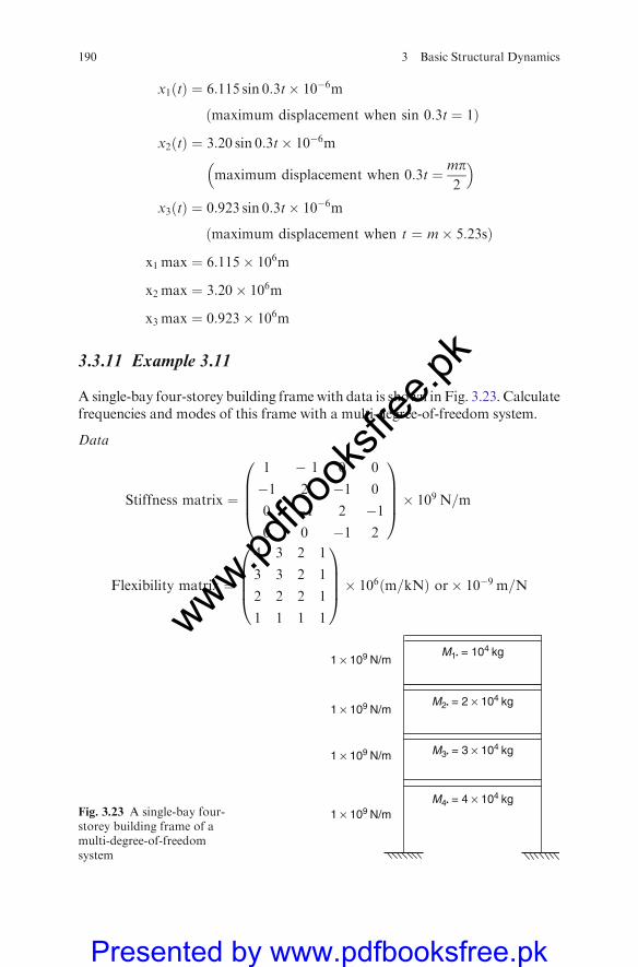
x1ðtÞ ¼ 6:115 sin 0:3t� 10�6m
ðmaximum displacement when sin 0:3t ¼ 1Þ
x2ðtÞ ¼ 3:20 sin 0:3t� 10�6m
maximum displacement when 0:3t ¼ mp2
� �
x3ðtÞ ¼ 0:923 sin 0:3t� 10�6m
ðmaximum displacement when t ¼ m� 5:23sÞ
x1 max ¼ 6:115� 106m
x2 max ¼ 3:20� 106m
x3 max ¼ 0:923� 106m
3.3.11 Example 3.11
A single-bay four-storey building frame with data is shown in Fig. 3.23. Calculatefrequencies and modes of this frame with a multi-degree-of-freedom system.
Data
Stiffness matrix ¼
1 � 1 0 0
�1 2 �1 0
0 �1 2 �10 0 �1 2
0BBB@
1CCCA� 109 N=m
Flexibility matrix ¼
4 3 2 1
3 3 2 1
2 2 2 1
1 1 1 1
0BBB@
1CCCA� 106ðm=kNÞ or� 10�9 m=N
M2• = 2 × 10⁴ kg
1 × 10⁹ N/m
1 × 10⁹ N/m
1 × 10⁹ N/m
1 × 10⁹ N/m
M1• = 104 kg
M3• = 3 × 10⁴ kg
M4• = 4 × 10⁴ kgFig. 3.23 A single-bay four-storey building frame of amulti-degree-of-freedomsystem
190 3 Basic Structural Dynamics
www.pdfbo
oksfr
ee.pk
Presented by www.pdfbooksfree.pk
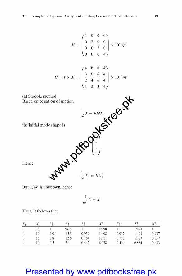
M ¼
1 0 0 0
0 2 0 0
0 0 3 0
0 0 0 4
0BBB@
1CCCA� 104 kg
H ¼ F�M ¼
4 6 6 4
3 6 6 4
2 4 6 4
1 2 3 4
0BBB@
1CCCA� 10�5m2
(a) Stodola methodBased on equation of motion
1
o2X ¼ FMX
the initial mode shape is
X01 ¼
1
1
1
1
0BBB@
1CCCA
Hence
1
o2X1
1 ¼ HX01
But 1=o2 is unknown, hence
1
o2X ¼ �X
Thus, it follows that
X01 X1
1 X11
�X21 X2
1�X31 X3
1�X41 X4
1
1 20 1 96.5 1 15.98 1 15.90 1
1 19 0.95 15.5 0.939 14.98 0.937 14.90 0.937
1 16 0.8 12.6 0.764 12.11 0.758 12.03 0.757
1 10 0.5 7.3 0.442 6.938 0.434 6.884 0.433
3.3 Examples of Dynamic Analysis of Building Frames and Their Elements 191
www.pdfbo
oksfr
ee.pk
Presented by www.pdfbooksfree.pk
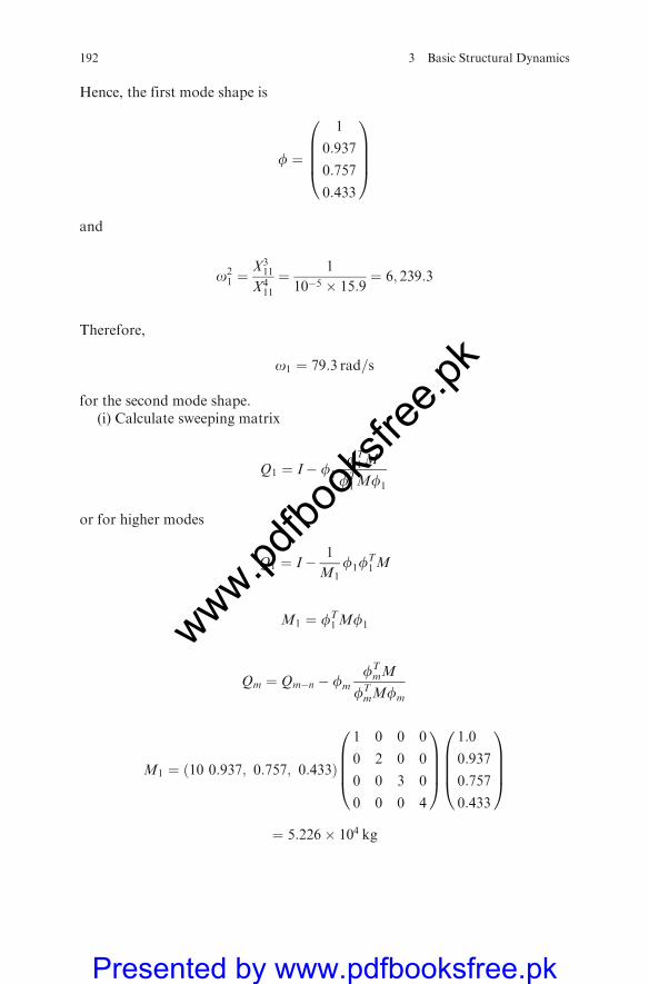
Hence, the first mode shape is
f ¼
1
0:937
0:757
0:433
0BBB@
1CCCA
and
o21 ¼
X311
X411
¼ 1
10�5 � 15:9¼ 6; 239:3
Therefore,
o1 ¼ 79:3 rad=s
for the second mode shape.(i) Calculate sweeping matrix
Q1 ¼ I� f1
fT1M
fT1Mf1
or for higher modes
Q1 ¼ I� 1
M1f1f
T1M
M1 ¼ fT1Mf1
Qm ¼ Qm�n � fm
fTmM
fTmMfm
M1 ¼ ð10 0:937; 0:757; 0:433Þ
1 0 0 0
0 2 0 0
0 0 3 0
0 0 0 4
0BBB@
1CCCA
1:0
0:937
0:757
0:433
0BBB@
1CCCA
¼ 5:226� 104 kg
192 3 Basic Structural Dynamics
www.pdfbo
oksfr
ee.pk
Presented by www.pdfbooksfree.pk
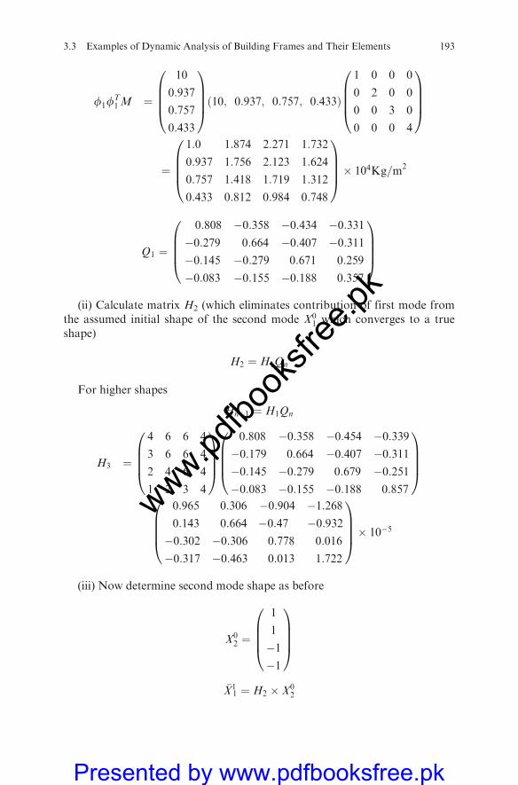
f1fT1M ¼
10
0:937
0:757
0:433
0BBB@
1CCCAð10; 0:937; 0:757; 0:433Þ
1 0 0 0
0 2 0 0
0 0 3 0
0 0 0 4
0BBB@
1CCCA
¼
1:0 1:874 2:271 1:732
0:937 1:756 2:123 1:624
0:757 1:418 1:719 1:312
0:433 0:812 0:984 0:748
0BBB@
1CCCA� 104Kg=m2
Q1 ¼
0:808 �0:358 �0:434 �0:331�0:279 0:664 �0:407 �0:311�0:145 �0:279 0:671 0:259
�0:083 �0:155 �0:188 0:357
0BBB@
1CCCA
(ii) Calculate matrix H2 (which eliminates contribution of first mode fromthe assumed initial shape of the second mode X0
1 which converges to a trueshape)
H2 ¼ H1Qn
For higher shapes
Hnþ1 ¼ H1Qn
H3 ¼
4 6 6 4
3 6 6 4
2 4 6 4
1 2 3 4
0BBB@
1CCCA
0:808 �0:358 �0:454 �0:339�0:179 0:664 �0:407 �0:311�0:145 �0:279 0:679 �0:251�0:083 �0:155 �0:188 0:857
0BBB@
1CCCA
0:965 0:306 �0:904 �1:2680:143 0:664 �0:47 �0:932�0:302 �0:306 0:778 0:016
�0:317 �0:463 0:013 1:722
0BBB@
1CCCA� 10�5
(iii) Now determine second mode shape as before
X02 ¼
1
1
�1�1
0BBB@
1CCCA
�X11 ¼ H2 � X0
2
3.3 Examples of Dynamic Analysis of Building Frames and Their Elements 193
www.pdfbo
oksfr
ee.pk
Presented by www.pdfbooksfree.pk
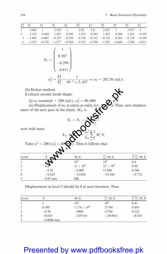
f2 ¼
1
0:587
�0:299
�0:811
0BBBBB@
1CCCCCA
o22 ¼
X42
�X52
¼ 1
10�5 � 2; 437) o2 ¼ 202:56 rad=s
(b) Holzer methodEvaluate second mode shape:
(i) o2 assumed = 200 rad/s, o22 ¼ 40; 000
(ii) Displacement of m1 is taken as unity (i.e. X1 ¼ 1). Thus, new displace-ment of the next pass in the chain, M2, is
X2 ¼ X1 � o2M1X1
k2
now with mass
Xm ¼ Xm�n �o2
km
Xm�nr¼1
M;X;
Take o2 ¼ 200 o22 ¼ 40; 000
� �. Then it follows that
Level X MrXr
PMrXr
o21
k
PMrXr
1 1 104 104 0.4
2 0.6 12 � 104 22 � 104 0.88
3 �0.28 �8,400 13,600 0.544
4 �0.824 �32,960 �19,360 �0.7745 0.05 mm OK
Displacement at level 5 should be 0 at next iteration. Thus
Level X MrXr
PMrXr
o21
km
PMrXr
1 1 104 104 0.41
2 0.589 1.178 � 104 21780 0.893
3 �0.30 �9000 12780 0.524
4 �0.824 �32974.8 �20194.8 �0.8285 �0.0046 mm
X02
�X12 X1
2�X22 X2
2�X32 X3
2�X42 X4
2�X52 X5
2
1 3.443 1 2.455 1 2.42 1.0 2.427 1 2.437 1
1 2.219 0.644 1.451 0.591 1.415 0.585 1.423 0.586 1.432 0.587
�1 �1.402 �0.407 �0.327 �0.336 �0.756 �0.312 �0.736 �0.303 �0.729 �0.299�1 �2.515 �0.730 �1.877 �0.765 �1.912 �0.790 �1.952 �0.804 �1.926 �0.811
194 3 Basic Structural Dynamics
www.pdfbo
oksfr
ee.pk
Presented by www.pdfbooksfree.pk
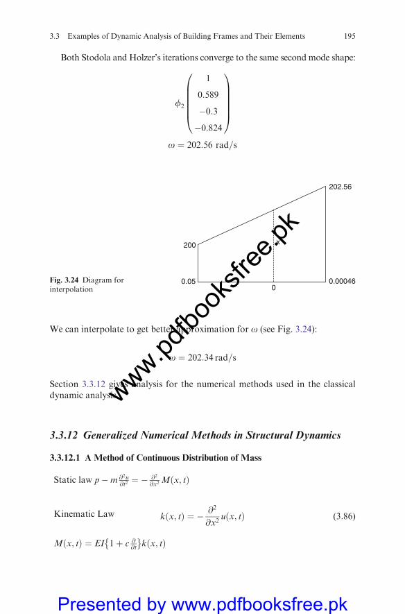
Both Stodola and Holzer’s iterations converge to the same second mode shape:
f2
1
0:589
�0:3
�0:824
0BBBBB@
1CCCCCA
o ¼ 202:56 rad=s
We can interpolate to get better approximation for o (see Fig. 3.24):
o ¼ 202:34 rad=s
Section 3.3.12 gives analysis for the numerical methods used in the classicaldynamic analysis.
3.3.12 Generalized Numerical Methods in Structural Dynamics
3.3.12.1 A Method of Continuous Distribution of Mass
Static law p�m @2u@t2¼ � @2
@x2Mðx; tÞ
Kinematic Law kðx; tÞ ¼ � @2
@x2uðx; tÞ (3:86)
Mðx; tÞ ¼ EI 1þ c @@t
kðx; tÞ
200
0.000460.05
202.56
0
x
Fig. 3.24 Diagram forinterpolation
3.3 Examples of Dynamic Analysis of Building Frames and Their Elements 195
www.pdfbo
oksfr
ee.pk
Presented by www.pdfbooksfree.pk
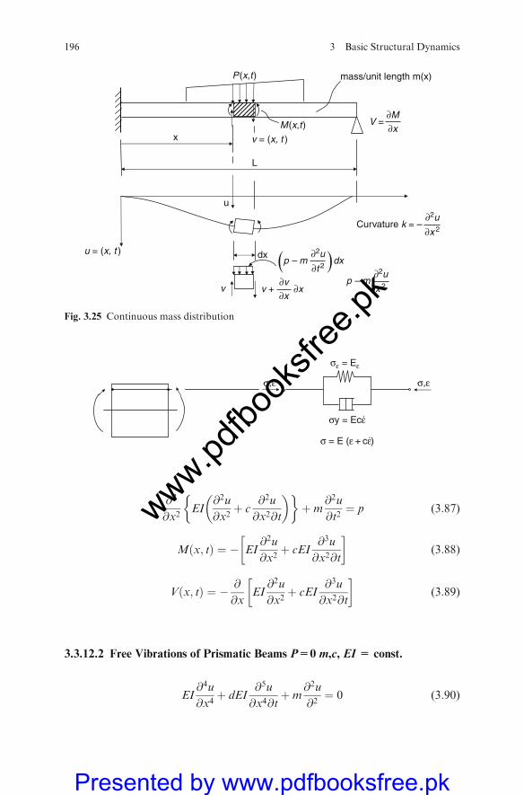
@2
@x2EI
@2u
@x2þ c
@2u
@x2@t
� �� �þm
@2u
@t2¼ p (3:87)
Mðx; tÞ ¼ � EI@2u
@x2þ cEI
@3u
@x2@t
�(3:88)
Vðx; tÞ ¼ � @
@xEI@2u
@x2þ cEI
@3u
@x2@t
�(3:89)
3.3.12.2 Free Vibrations of Prismatic Beams P=0 m,c, EI = const.
EI@4u
@x4þ dEI
@5u
@x4@tþm
@2u
@2¼ 0 (3:90)
L
v = (x, t )
u = (x, t )
M(x,t)x
mass/unit length m(x)P(x,t)
dx
u
Curvature k = –
V = ∂M
∂x
∂2u
∂x 2
v + v∂v
∂x∂x
∂2u
∂t 2p – m
∂2u
∂x 2 p – m
dx
Fig. 3.25 Continuous mass distribution
σ = E (ε + cε.)
σy = Ecε.
σε = Eε
σ,ε σ,ε
196 3 Basic Structural Dynamics
www.pdfbo
oksfr
ee.pk
Presented by www.pdfbooksfree.pk
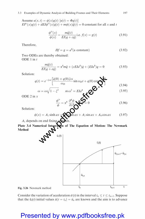
Assume uðx; tÞ ¼ fðxÞqðtÞ ½uðtÞ ¼ FqðtÞ�EIivðxÞqðtÞ þ dEIfivðxÞ _qðtÞ þmfðxÞ€qðtÞ ¼ 0 constant for all x and t
fivðxÞfðxÞ ¼
m€qðtÞEIðqþ c _qÞ i:e: fðxÞ ¼ gðtÞ (3:91)
Therefore,
Hf ¼ g ¼ a4ða constantÞ (3:92)
Two ODEs are thereby obtained:ODE 1 in t
m€qðtÞEIðqþ e _qÞ ¼ a4m€qþ ðcEIa4Þ _qþ ðEIa4Þq ¼ 0 (3:93)
Solution:
qðtÞ ¼ e�xot_qð0Þ þ qð0Þxo
oDsinoDtþ qð0Þ cosoDt
�
o ¼ offiffiffiffiffiffiffiffiffiffiffiffiffi1� x2
qmo2 ¼ EIa4 ð3:95Þ
(3:94)
ODE 2 in x
fiv
f¼ a4
@4f@x4� a4f ¼ 0 (3:96)
Solution:
fðxÞ ¼ A1 sinh axþ A2 cosh axþ A3 sin axþ A4 cos ax (3:97)
A1 depends on end fixing of beam.
Plate 3.4 Numerical Integration of The Equation of Motion: The Newmark
Method
Consider the variation of acceleration u (t) in the interval tn � t � tnþ1. Supposethat the ui(t) initial values €uðt ¼ tnÞ ¼ €un are known and the aim is to advance
ü,(t)
f,(t)
tn tn+1 t
üt,n
üt,n+1– üt,n
Fig. 3.26 Newmark method
3.3 Examples of Dynamic Analysis of Building Frames and Their Elements 197
www.pdfbo
oksfr
ee.pk
Presented by www.pdfbooksfree.pk
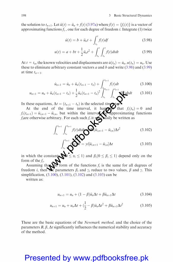
the solution to tnþ1. Let €uðtÞ ¼ €un þ fðtÞ (3.97a) where fðtÞ ¼ ffiðtÞg is a vector ofapproximating functions fi , one for each degree of freedom i. Integrate (1) twice
_uðtÞ ¼ bþ €untþZ t
tn
fðtÞdf (3:98)
uðtÞ ¼ aþ btþ 1
2€unt
2 þZ t
tn
Z t
tn
fðtÞdtdt (3:99)
At t= tn, the known velocities and displacements are _uðtnÞ ¼ _un; uðtnÞ ¼ un. Usethese to eliminate arbitrary constant vectors a and b and write (3.98) and (3.99)at time tn+1.
_unþ1 ¼ _un þ €unðtnþ1 � tnÞ þZ tnþ1
tn
fðtÞdt (3:100)
unþ1 ¼ un þ €unðtnþ1 � tnÞ þ1
2€unðtnþ1 � tnÞ2
Z tnþ1
tn
Z tnþ1
tn
fðtÞdtdt (3:101)
In these equations, Dt ¼ ðtnþ1 � tnÞ is the selected time-step.At the end of the time interval, it happens that fiðtnÞ ¼ 0 and
fiðtnþ1Þ ¼ €ui;nþ1 � €ui;n, but within the interval the approximating functionsfiare otherwise arbitrary. For each such fi it may easily be written as
Z tnþ1
tn
Z tnþ1
tn
fðtÞdtdt ¼ Bið€ui;nþ1 � €ui;nÞDt2 (3:102)
Z tnþ1
tn
fiðtÞdt ¼ yi½€ui;nþ1 � €ui;n�Dt (3:103)
in which the constants aið0 � ai � 1Þ and bið0 � bi � 1Þ depend only on theform of the fi.
Assuming that the form of the functions fi is the same for all degrees offreedom i, then the parameters bi and gi reduce to two values, b and g. Thissimplification, (3.100), (3.101), (3.102) and (3.103) can be
written as:
unþ1 ¼ un þ ð1� bÞ€unDtþ b€unþ1Dt (3:104)
unþ1 ¼ un þ unDtþ ð1
2� bÞ€unDt2 þ b€unþ1Dt2 (3:105)
These are the basic equations of the Newmark method, and the choice of theparameters B, b, Dt significantly influences the numerical stability and accuracyof the method.
198 3 Basic Structural Dynamics
www.pdfbo
oksfr
ee.pk
Presented by www.pdfbooksfree.pk

From Eq. (3.105) the incremental acceleration vector is obtained:
D€u ¼ €unþ1 � €un ¼1
bDt2½unþ1; � un� �
1
bDtun �
1
2b€un (3:106)
Now substitute Eq. (3.106) to Eq. (3.104) gives the incremental velocityvector:
D _u ¼ _unþ1 � _un ¼g
bDt½unþ1 � un� �
gb
_un þ ð1�g2bÞ€unDt (3:107)
At times tn+1 and tn, the equations of motion may be written as:
m€unþ1 þ cunþ1 þ kunþ1 ¼ pnþ1 (3:108)
m€un þ cun þ kun ¼ pn (3:109)
Subtracting Eqs. (3.108) and (3.109) the equations of motion in incrementalform can be written as
mD€uþ cD _uþ kDu ¼ Dp (3:110)
When Eqs (3.106) and (3.107) are substituted into (3.108) gives the incrementaldisplacements:
1
aDt2mþ y
aDtcþ k
�Du ¼ Dpþ 1
aDtmþ y
ac
�_uuþ
1
2amþ y
2a
n oDtc
�€un (3:111)
Algorithm
For a structure having N degrees of freedom, choose the time step Dt ¼ 0:1TN,where TN is the shortest natural period. Choose the parameters a = 0.25(constant average acceleration) and b = 0.5 (no algorithmic damping).
Plate No. 3.5 Eigenvalue analysis by inverse matrix iteration
In structural dynamics, the ith natural circular frequency oi and natural modefi must satisfy
kfi ¼ o2imfi (3:112)
Let s be a constant called the shift. Then, subtracting smfi from both sides ofEq. (1) gives
k� sm½ �fi ¼ ðo2i � sÞmfi (3:113)
The modified stiffness matrix retains the same eigenvectors fi but shifts all theeigenvalues o2
i by the same amount s.
3.3 Examples of Dynamic Analysis of Building Frames and Their Elements 199
www.pdfbo
oksfr
ee.pk
Presented by www.pdfbooksfree.pk
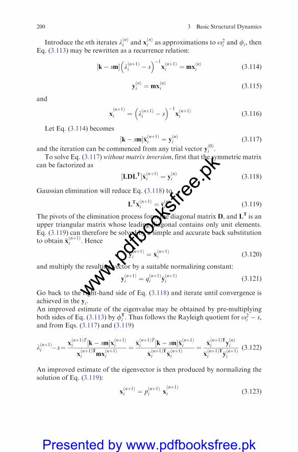
Introduce the nth iterates lðnÞi and xðnÞi as approximations to o2
i and fi, thenEq. (3.113) may be rewritten as a recurrence relation:
½k� sm� lðnþ1Þi � s� ��1
xðnþ1Þi ¼ mx
ðnÞi (3:114)
yðnÞi ¼ mx
ðnÞi (3:115)
and
xðnþ1Þi ¼ lðnþ1Þi � s
� ��1xðnþ1Þi (3:116)
Let Eq. (3.114) becomes
½k� sm��xðnþ1Þi ¼ yðnÞi (3:117)
and the iteration can be commenced from any trial vector yð0Þi .
To solve Eq. (3.117) without matrix inversion, first that the symmetric matrixcan be factorized as
½LDLT��xðnþ1Þi ¼ yðnÞi (3:118)
Gaussian elimination will reduce Eq. (3.118) to
LT�xðnþ1Þi ¼ �v
ðnÞi (3:119)
The pivots of the elimination process form the diagonal matrix D, and LT is anupper triangular matrix whose leading diagonal contains only unit elements.Eq. (3.119) can therefore be solved by a simple and accurate back substitutionto obtain �x
ðnþ1Þi . Hence
�yðnþ1Þi ¼ �x
ðnþ1Þi (3:120)
and multiply the resulting vector by a suitable normalizing constant:
yðnþ1Þi ¼ q
ðnþ1Þi �y
ðnþ1Þi (3:121)
Go back to the right-hand side of Eq. (3.118) and iterate until convergence isachieved in the yi.An improved estimate of the eigenvalue may be obtained by pre-multiplyingboth sides of Eq. (3.113) by fT
i . Thus follows the Rayleigh quotient for o2i � s,
and from Eqs. (3.117) and (3.119)
lðnþ1Þi �s¼ xðnþ1ÞTi ½k� sm�xðnþ1Þi
xðnþ1ÞTi mx
ðnþ1Þi
¼ �xðnþ1ÞTi ½k� sm��xðnþ1Þi
�xðnþ1ÞTi �x
ðnþ1Þi
¼ �xðnþ1ÞTi y
ðnÞi
�xðnþ1ÞTi �y
ðnþ1Þi
(3:122)
An improved estimate of the eigenvector is then produced by normalizing thesolution of Eq. (3.119):
xðnþ1Þi ¼ p
ðnþ1Þi x
ðnþ1Þi (3:123)
200 3 Basic Structural Dynamics
www.pdfbo
oksfr
ee.pk
Presented by www.pdfbooksfree.pk
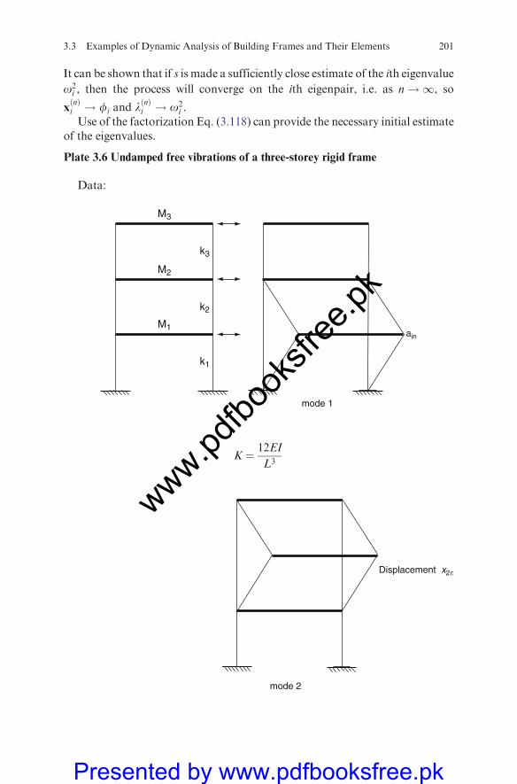
It can be shown that if s is made a sufficiently close estimate of the ith eigenvalue
o2i , then the process will converge on the ith eigenpair, i.e. as n!1, so
xðnÞi ! fi and lðnÞi ! o2
i .
Use of the factorization Eq. (3.118) can provide the necessary initial estimate
of the eigenvalues.
Plate 3.6 Undamped free vibrations of a three-storey rigid frame
Data:
K ¼ 12EI
L3
mode 1
M3
M2
M1
k3
k2
k1
ain
mode 2
Displacement x2n
3.3 Examples of Dynamic Analysis of Building Frames and Their Elements 201
www.pdfbo
oksfr
ee.pk
Presented by www.pdfbooksfree.pk
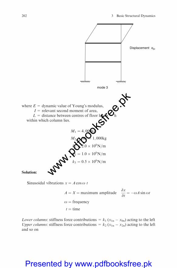
where E = dynamic value of Young’s modulus,I = relevant second moment of area,L = distance between centres of floor levels = h
within which column lies.
M1 ¼ 4; 000kg
M2 ¼M3 ¼ 1; 000kg
k1 ¼ 2:0� 106N=m
k2 ¼ 1:0� 106N=m
k3 ¼ 0:5� 106N=m
Solution:
Sinusoidal vibrations x ¼ A coso t
A ¼ X ¼ maximum amplitudedxdt¼ �oA sinot
o ¼ frequency
t ¼ time
Lower columns: stiffness force contributions = k1 (x1n � x0n) acting to the leftUpper columns: stiffness force contributions = k2 (x1n � x2n) acting to the left
and so on
mode 3
Displacement x3n
202 3 Basic Structural Dynamics
www.pdfbo
oksfr
ee.pk
Presented by www.pdfbooksfree.pk
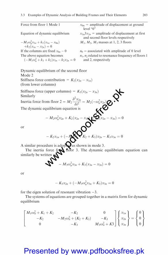
Dynamic equilibrium of the second floorMode 2Stiffness force contribution = K2ðx2n � x1nÞ(from lower columns)
Stiffness force (upper columns) = K3ðx2n � x3nÞSimilarly
Inertia force from floor 2 ¼M2d2x2ndt2¼M2ð�o2
nx2nÞ
The dynamic equilibrium equation is
�M2o2nx2n þ K2ðx2n � x1nÞ þ K3ðx2n � x3nÞ ¼ 0
or
� K2x1n þ ð�M2o2n þ K2 þ K3Þx2n � K3x3n ¼ 0
A similar procedure is adopted as shown in mode 3.The inertia force from floor 3. The dynamic equilibrium equation can
similarly be written as
�M3o2nx3n þ K3ðx3n � x2nÞ ¼ 0
or
� K3x2n þ ð�M3o2nx3n þ K3Þx3n ¼ 0
for the eigen solution of resonant vibration �3.The systems of equations are grouped together in a matrix form for dynamic
equilibrium
M1o2n þ K1 þ K2 �K2 0
�K2 �M2o2n þ ðK2 þ K3Þ �K3
0 �K3 M3o2n þ K3
264
375
x1n
x2n
x3n
8><>:
9>=>; ¼
0
0
0
8><>:
9>=>;
Force from floor 1 Mode 1 x0n = amplitude of displacement at groundlevel ‘‘0’’
Equation of dynamic equilibrium x1n3x2n = amplitude of displacement at firstand second floor levels respectively
�M1o2nx1n þ k1ðx1n � x0nÞ
þk2ðx1n � x2nÞ ¼ 0M1, M2, M3 masses at 1, 2, 3 floors
If the columns are fixed x0n � 0 n0 ¼ associated with amplitude of 0 level
The above equation becomes
ð�M1o2n þ k1 þ k2Þx1n � k2x2n ¼ 0
n1, n2 related to resonance frequency of floors 1
and 2, respectively
3.3 Examples of Dynamic Analysis of Building Frames and Their Elements 203
www.pdfbo
oksfr
ee.pk
Presented by www.pdfbooksfree.pk
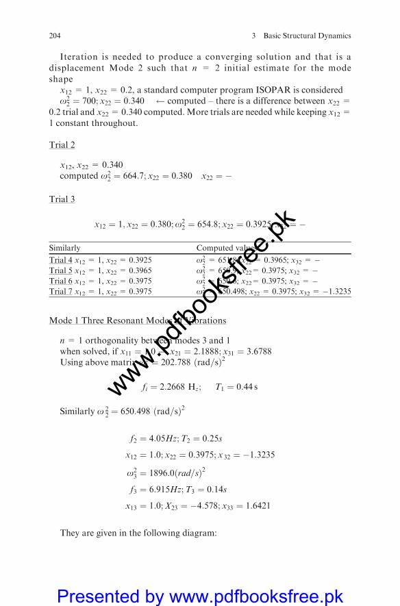
Iteration is needed to produce a converging solution and that is a
displacement Mode 2 such that n = 2 initial estimate for the mode
shapex12 = 1, x22 = 0.2, a standard computer program ISOPAR is consideredo2
2 ¼ 700; x22 ¼ 0:340 computed – there is a difference between x22 =
0.2 trial and x22 = 0.340 computed. More trials are needed while keeping x12=
1 constant throughout.
Trial 2
x12, x22 = 0.340computed o2
2 ¼ 664:7; x22 ¼ 0:380 x22 ¼ �
Trial 3
x12 ¼ 1; x22 ¼ 0:380;o22 ¼ 654:8; x22 ¼ 0:3925; x32 ¼ �
Similarly Computed values
Trial 4 x12 = 1, x22 = 0.3925 o22 = 651.8; x22 = 0.3965; x32 = �
Trial 5 x12 = 1, x22 = 0.3965 o22 = 650.9; x22= 0.3975; x32 = �
Trial 6 x12 = 1, x22 = 0.3975 o22 = 650.6; x22= 0.3975; x32 = �
Trial 7 x12 = 1, x22 = 0.3975 o22 = 650.498; x22 = 0.3975; x32 = �1.3235
Mode 1 Three Resonant Modes of Vibrations
n = 1 orthogonality between modes 3 and 1when solved, if x11 ¼ 1:0! x21 ¼ 2:1888; x31 ¼ 3:6788Using above matrix o2
1 ¼ 202:788 ðrad=sÞ2
fi ¼ 2:2668 Hz; T1 ¼ 0:44 s
Similarly o 22¼ 650:498 ðrad=sÞ2
f2 ¼ 4:05Hz;T2 ¼ 0:25s
x12 ¼ 1:0; x22 ¼ 0:3975; x 32 ¼ �1:3235
o23 ¼ 1896:0ðrad=sÞ2
f3 ¼ 6:915Hz;T3 ¼ 0:14s
x13 ¼ 1:0;X23 ¼ �4:578; x33 ¼ 1:6421
They are given in the following diagram:
204 3 Basic Structural Dynamics
www.pdfbo
oksfr
ee.pk
Presented by www.pdfbooksfree.pk
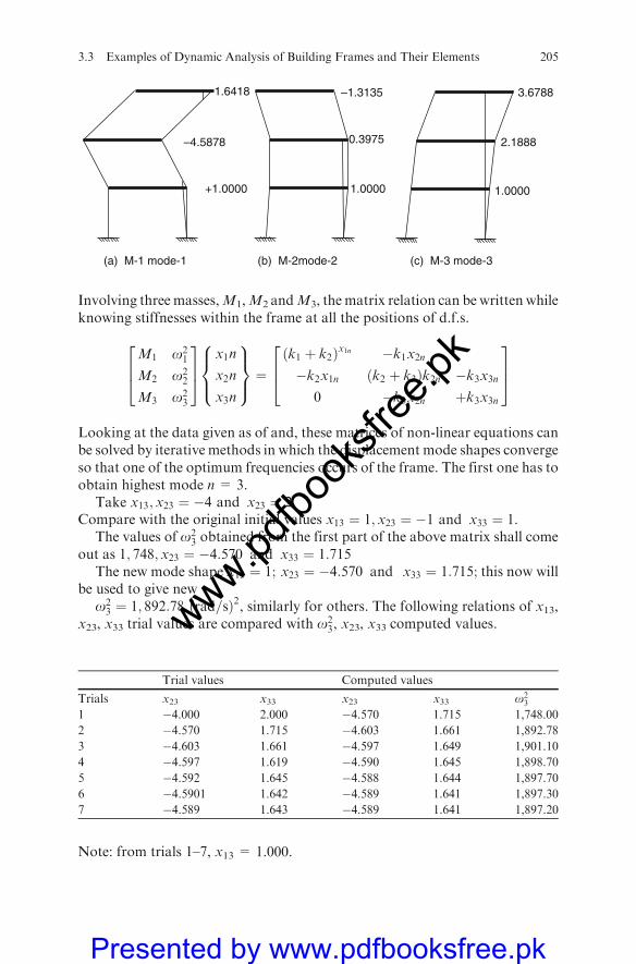
Involving three masses,M1,M2 andM3, thematrix relation can be written whileknowing stiffnesses within the frame at all the positions of d.f.s.
M1 o21
M2 o22
M3 o23
264
375
x1n
x2n
x3n
8><>:
9>=>; ¼
ðk1 þ k2Þx1n �k1x2n�k2x1n ðk2 þ k3Þk2n �k3x3n
0 �k3x2n þk3x3n
264
375
Looking at the data given as of and, these matrices of non-linear equations canbe solved by iterative methods in which the displacement mode shapes convergeso that one of the optimum frequencies occurs of the frame. The first one has toobtain highest mode n = 3.
Take x13; x23 ¼ �4 and x23 ¼ 2:Compare with the original initial values x13 ¼ 1; x23 ¼ �1 and x33 ¼ 1.
The values of o23 obtained from the first part of the above matrix shall come
out as 1; 748; x23 ¼ �4:570 and x33 ¼ 1:715The new mode shape x13 ¼ 1; x23 ¼ �4:570 and x33 ¼ 1:715; this now will
be used to give newo2
3 ¼ 1; 892:78 ðrad=sÞ2, similarly for others. The following relations of x13,x23, x33 trial values are compared with o2
3, x23, x33 computed values.
Note: from trials 1–7, x13 = 1.000.
(a) M-1 mode-1
1.6418 –1.3135
–4.5878
+1.0000
2.18880.3975
1.0000
3.6788
1.0000
(b) M-2mode-2 (c) M-3 mode-3
Trial values Computed values
Trials x23 x33 x23 x33 o23
1 �4.000 2.000 �4.570 1.715 1,748.00
2 �4.570 1.715 �4.603 1.661 1,892.78
3 �4.603 1.661 �4.597 1.649 1,901.10
4 �4.597 1.619 �4.590 1.645 1,898.70
5 �4.592 1.645 �4.588 1.644 1,897.70
6 �4.5901 1.642 �4.589 1.641 1,897.30
7 �4.589 1.643 �4.589 1.641 1,897.20
3.3 Examples of Dynamic Analysis of Building Frames and Their Elements 205
www.pdfbo
oksfr
ee.pk
Presented by www.pdfbooksfree.pk

Similarly using the above matrix with the iterative technique indicated the
above values are computed for x23, x33 x23 and o23 and they are tabulated.
The mass orthogonality between modes 3 and 2. The equation set up is M1 x12x13+M2 x22 x23+M3 x32 x33= 0. Substituting values, then the relation can be
easily found between x32 to x12 and x22, x32 to x12 and x22The value of x3 can be determined.
206 3 Basic Structural Dynamics
www.pdfbo
oksfr
ee.pk
Presented by www.pdfbooksfree.pk
Chapter 4
Earthquake Response Spectra With Coded
Design Examples
4.1 Introduction
The most important application in structural dynamics is in the analysis of theresponse of structures to ground shaking caused by an earthquake. The earth-quake response is generally divided into two categories – linearly elastic andinelastic.
The response spectrum concept which is central to earthquake engineeringtogether with procedures to evaluate the peak response of systems directly formthe response spectrum. This then is followed by a study of the characteristicsof the earthquake response spectra which generally lead into the design spec-trum for the design of new buildings and safety evaluation of existing buildingsagainst future earthquakes. The designers would be interested in response ofyielding or inelastic system.
The ground acceleration is defined by numerical values at discrete timeinstants. These time instants should be closely spaced to describe accuratelythe highly irregular variation of acceleration with time. Typically, the timeinterval is chosen to be 1/100 to 1/50 of a second, requiring 1,500–3,000ordinates to describe the ground motion.
The main cause of the structural damage during earthquake is its response toground motions which is, in fact the input to the base of the structure. Toevaluate the behaviour of the building under this type of loading condition,knowledge of structural dynamics is required. The static analysis and design cannow be changed to a separate time-dependent analysis and design. The loadingand all aspects of responses vary with time which result in an infinite number ofpossible solutions at each instant during the time interval. For an engineer themaximum values of the building response are needed for the structural design.
The response may be deflection, shear, equivalent acceleration, etc. Theresponse curves are generally similar with a major variation occurring inthe vertical ordinates. The variations definitely occur with the magnitude ofthe earthquake and location of the recording instruments. Accelerationsderived from actual earthquakes are surprisingly high as compared with theforce used in designs and the main reason is the effect of different degrees ofdamping.
M.Y.H. Bangash, Earthquake Resistant Buildings,DOI 10.1007/978-3-540-93818-7_4, � M.Y.H. Bangash 2011
207
www.pdfbo
oksfr
ee.pk
Presented by www.pdfbooksfree.pk
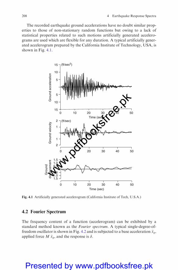
The recorded earthquake ground accelerations have no doubt similar prop-
erties to those of non-stationary random functions but owing to a lack of
statistical properties related to such motions artificially generated accelero-
grams are used which are flexible for any duration. A typical artificially gener-
ated accelerogram prepared by the California Institute of Technology, USA, is
shown in Fig. 4.1.
4.2 Fourier Spectrum
The frequency content of a function (accelerogram) can be exhibited by a
standard method known as the Fourier spectrum. A typical single-degree-of-
freedom oscillator is shown in Fig. 4.2 and is subjected to a base acceleration €xg,applied force M €xg, and the response is d.
15 (ft/sec2)
(ft/sec)
(ft)
10
5
5
10Gro
und
acce
lera
tion
Gro
und
velo
city
Gro
und
dis
plac
emen
t
150
2
1.51.00.5
0.51.01.5
1
1
2
0 10 20 30 40 50
0 10 20Time (sec)
30 40 50
10Time (sec)
20 30 40 50
Fig. 4.1 Artificially generated accelerogram (California Institute of Tech, U.S.A.)
208 4 Earthquake Response Spectra
www.pdfbo
oksfr
ee.pk
Presented by www.pdfbooksfree.pk

The equation of motion is
M€dþ Kd ¼ �M€xg (4:1)
where d is the relative displacement and €w is the base acceleration.The vibratory response is given for the relative displacement at time ‘t’ by
dðt;oÞ ¼ 1
o
Z t
0
€xgðtÞ sinoðt� tÞdt (4:2)
o2 ¼ K
M¼ 2p
TZ
� �2
where T is the period.The total energy is
E ¼ 1
2M _d2 þ 1
2Kd2 (4:3)
¼ 1
2M
Z t
0
€xg sinotdt� �2
þZ t
0
€xg cosotdt� �" #2
(4:4)
The duration of €w from t ¼ 0 to t ¼ t1, the square root of twice the energy perunit mass at that time t1, is
ffiffiffiffiffiffiffiffiffiffiffiffiffiffiffiffiffi2Eðt;oÞ
M
r¼
Z t
0
€xg sinotdt� �2
þZ t1
0
€xg cosotdt� �2
" #1=2(4:5)
where
o ¼ 2pTZ¼ 2pf
Mδ δ
M
KK
Mx..
xg..
Fig. 4.2 A single-degree-of-freedom oscillator
4.2 Fourier Spectrum 209
www.pdfbo
oksfr
ee.pk
Presented by www.pdfbooksfree.pk
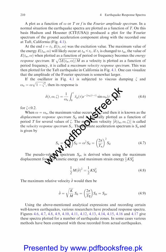
A plot as a function of o or T or f is the Fourier amplitude spectrum. In anormal situation the earthquake spectra are plotted as a function of T. On thisbasis Hudson and Housner (CIT(USA)) produced a plot for the Fourierspectrum of the ground acceleration component along with the recorded oneat Taft, California (Fig. 4.1).
At the end t ¼ t1;Eðt1;oÞ was the excitation value. The maximum value ofthe energy Eðtm;oÞ will likely occur at tm5t1. if t1 is changed to tm, the value ofEðtm;oÞ when plotted as a function of period or frequency becomes the energy
response spectrum. Ifffiffiffiffiffiffiffiffiffiffiffiffiffiffiffiffiffiffiffiffiffiffiffiffiffiffiffi2E tm;oð Þ=M
pas a velocity is plotted as a function of
period frequency, it is called a maximum velocity response spectrum. This wasthen plotted for the Taft earthquake in California in Fig. 4.1. One can visualizethat the amplitude of the Fourier spectrum is somewhat larger.
If the oscillator in Fig. 4.1 is subjected to viscous damping z and
on ¼ offiffiffiffiffiffiffiffiffiffiffiffiffi1� z2
p, then its response is
d t;o; zð Þ ¼ 1
on
Z t
0
€xg tð Þe�zon t�tð Þ sinon t� tð Þdt (4:6)
for z<0.2.When o ¼ on, the maximum value occurs at tm, and then it is known as the
displacement response spectrum Sd and is generally plotted as a function ofperiod T for several values of z. The maximum velocity _d tm;o; zð Þ
�� �� is calledthe velocity response spectrum Sv. The absolute acceleration spectrum is Sa andis given by
Sa ¼K
M
� �Sd ¼ o2Sd ¼
2pTn
� �2
Sd (4:7)
The pseudo-velocity spectrum Spv is derived when using the maximumdisplacement for zero kinetic energy and maximum strain energy 1
2KS2
d
1
2Mð _dÞ2 ¼ 1
2KS2
d (4:8)
The maximum relative velocity _d would then be
_d ¼ffiffiffiffiffiK
M
rSd ¼
2pTZ
� �Sd ¼ Spv (4:9)
Using the above-mentioned analytical expressions and recording certainwell-known earthquakes, various researchers have produced response spectra.Figures 4.6, 4.7, 4.8, 4.9, 4.10, 4.11, 4.12, 4.13, 4.14, 4.15, 4.16 and 4.17 givethese spectra plotted for a number of earthquake zones. In some cases variousmethods have been compared with those recorded from actual earthquakes.
210 4 Earthquake Response Spectra
www.pdfbo
oksfr
ee.pk
Presented by www.pdfbooksfree.pk
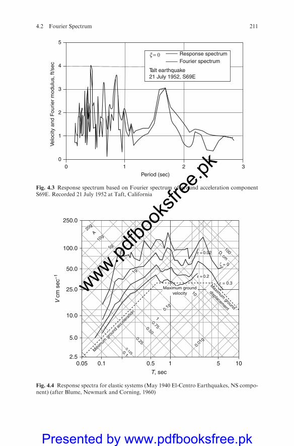
5
4
3
2
1
00 1
Period (sec)
Response spectrum Fourier spectrum
Talt earthquake21 July 1952, S69E
Velo
city
and
Fou
rier
mod
ulus
, ft/s
ec
32
= 0 ξ
Fig. 4.3 Response spectrum based on Fourier spectrum of ground acceleration componentS69E. Recorded 21 July 1952 at Taft, California
0.052.5
5.0
10.0
25.0
50.0
100.0
250.0
0.1 0.5
T, sec
V c
m s
ec–1
1 5 10
0.1
0.125
0.25
0.50
0.75
Maxim
um ground
displacement
10
100D, cm
1
Maximum groundvelocity
ε = 0.3
ζ = 0
ε = 0.2
ε = 0.02
0.01
g
0.1g
1g
5g10
g
20g
A
Mini
mum
gro
und
acce
lerat
ion
Fig. 4.4 Response spectra for elastic systems (May 1940 El-Centro Earthquakes, NS compo-nent) (after Blume, Newmark and Corning, 1960)
4.2 Fourier Spectrum 211
www.pdfbo
oksfr
ee.pk
Presented by www.pdfbooksfree.pk
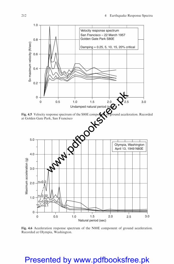
1.0
Velocity response spectrumSan Francisco – 22 March 1957Golden Gate Park S80E
Damping = 0.25, 5, 10, 15, 20% critical
0.8
0.6
0.4
0.2
0
0
Undamped natural period (sec)
Sv
max
imum
vel
ocity
(ft/
sec)
0.5 1.0 1.5 2.0 2.5 3.0
Fig. 4.5 Velocity response spectrum of the S80E component of ground acceleration. Recordedat Golden Gate Park, San Francisco
5.0
4.0
3.0
2.0
1.0
00 0.5 1.0
Natural period (sec)
Max
imum
acc
eler
atio
n (g
)
1.5 2.0 2.5 3.0
April 13, 1949 N80EOlympia, Washington
n=0.0
n=0.02
n=0.05n=0.1
Fig. 4.6 Acceleration response spectrum of the N80E component of ground acceleration.Recorded at Olympia, Washington.
212 4 Earthquake Response Spectra
www.pdfbo
oksfr
ee.pk
Presented by www.pdfbooksfree.pk
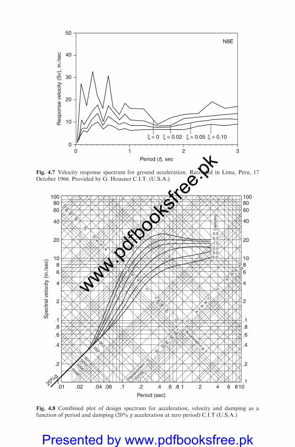
0.0
Dam
ping
1.02.05.0
10.0
0.5
10080
60
40
20
108
64
2
1.8
.6
.4
.2
.1.0
8
.06
.04
.02
.01
.02
.03
.04
.06
.08.1
.2
.4
.6.8
1
2
46
810
.003.002
.001.0005.0006.0008
Acceleration g, s
Displac
emen
t
inche
s
.01.1
.2
.4
.6
.8
.1
2
4
68
10
20
Spe
ctra
l vel
ocity
(in
./sec
)
40
6080
100
.1
.2
.4
.6
.8
.1
2
4
6810
200.0
Dam
ping
1.02.05.0
10.0
0.5
60
40
80100
20%
g
.02 .04 .06 .1 .2
Period (sec)
.4 .6 .8 1 2 4 6 108
10080
60
40
20
108
64
2
1.8
.6
.4
.2
.1.0
8
.06
.04
.02
.01
.02
.03
.04
.06
.08.1
.2
.4
.6.8
1
2
46
810
.003.002
.001.0005.0006.0008
Acceleration g, s
Displac
emen
t
inche
s
Fig. 4.8 Combined plot of design spectrum for acceleration, velocity and damping as afunction of period and damping (20% g acceleration at zero period) C.I.T (U.S.A.)
50
40
30
20
10
010
Period (t), sec
Res
pons
e ve
loci
ty (
Sv)
, in.
/sec
2
N8E
3
ξ = 0 ξ = 0.02 ξ = 0.05 ξ = 0.10
Fig. 4.7 Velocity response spectrum for ground acceleration. Recorded in Lima, Peru, 17October 1966. Provided by G. Housner C.I.T. (U.S.A.)
www.pdfbo
oksfr
ee.pk
Presented by www.pdfbooksfree.pk
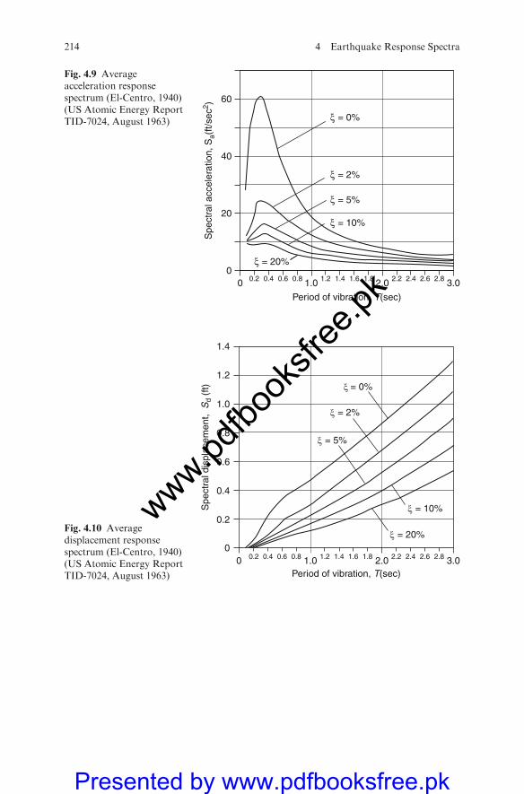
Spe
ctra
l acc
eler
atio
n, S
a(ft/
sec2 )
ξ = 0%
ξ = 2%
ξ = 5%
ξ = 10%
ξ = 20%0
Period of vibration, T(sec)
0 1.0 2.0 3.00.2 0.4 0.6 0.8 1.2 1.4 1.6 1.8 2.2 2.4 2.6 2.8
60
40
20
Fig. 4.9 Averageacceleration responsespectrum (El-Centro, 1940)(US Atomic Energy ReportTID-7024, August 1963)
0.2
0
Period of vibration, T(sec)
Spe
ctra
l dis
plac
emen
t, S
d (f
t)
0 1.0 2.0 3.00.2 0.4 0.6 0.8 1.2 1.4 1.6 1.8 2.2 2.4 2.6 2.8
1.4
1.2
1.0
0.8
0.6
0.4
ξ = 0%
ξ = 2%
ξ = 5%
ξ = 10%
ξ = 20%Fig. 4.10 Averagedisplacement responsespectrum (El-Centro, 1940)(US Atomic Energy ReportTID-7024, August 1963)
214 4 Earthquake Response Spectra
www.pdfbo
oksfr
ee.pk
Presented by www.pdfbooksfree.pk
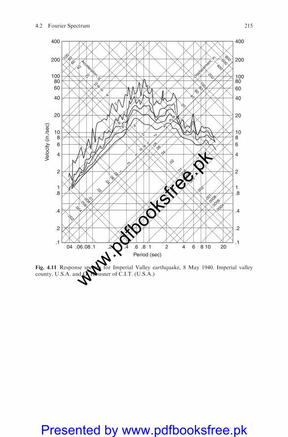
.002
.004
.006
.008.01
.02
.04
.06
.08.1
.2
.4
.000
4.000
6.000
8.0
01.0
02.0
04.006.0
08.01
.02
.04
.06.0
8
.2
.4.6.8
1
2
46
810
20 Displac
emen
t, in.
4060
80100
.6.8
1
2
4
6
Acceleration, g
20
40
6080
100
200
400
600
800
04 .06.08 .1 .2 .4 .6 .8
Period (sec)
Vel
ocity
(in
./sec
)
.1
.2
.4
.81
2
4
6
10
20
40
6080
100
200
.002
.004
.006
.008.01
.02
.04
.06
.08.1
.2
.4
.000
4.000
6.000
8.001
.002
.004
.006.0
08.01
.02
.04
.06.0
8
.2
.4.6.8
1
2
46
810
20 Displac
emen
t, in.
4060
80100
.6.8
1
2
4
6
Acceleration, g
20
40
6080
100
200
400
600
800
400
8
.1
.2
.4
.81
2
4
6
10
20
40
6080100
200
400
8
1 2 4 6 8 10 20
810
810
Fig. 4.11 Response spectra for Imperial Valley earthquake, 8 May 1940. Imperial valleycounty, U.S.A. and G. Housner of C.I.T. (U.S.A.)
4.2 Fourier Spectrum 215
www.pdfbo
oksfr
ee.pk
Presented by www.pdfbooksfree.pk
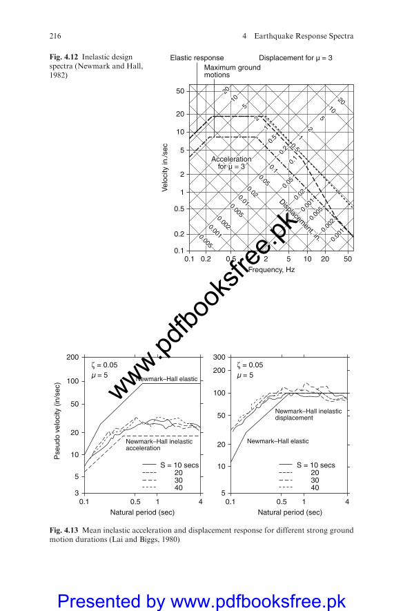
0.10.1
0.2
0.5
1
2
5
10
20
50
Elastic responseMaximum groundmotions
Displacement for µ = 3
0.2 0.5 1 2
Frequency, Hz
Vel
ocity
in./s
ec
5 10 20 50
Accelerationfor µ = 3
0.00
10.00
20.00
50.00
10.02
0.05
0.1
0.2
0.5
1
2
510
20
0.005
0.001
0.002
0.005
0.01
0.02Displacem
ent, in.
0.05
0.1
0.5
12
5
10
20
Accelerationfor µ = 3
0.00
10.00
20.00
50.00
10.02
0.05
0.1
0.2
0.5
1
2
510
20
0.005
0.001
0.002
0.005
0.01
0.02Displacem
ent, in.
0.05
0.1
0.5
12
5
10
20
Fig. 4.12 Inelastic designspectra (Newmark and Hall,1982)
S = 10 secs
Newmark–Hall inelasticacceleration
Natural period (sec) Natural period (sec)
Newmark–Hall inelasticdisplacement
Newmark–Hall elastic
Newmark–Hall elastic
203040
S = 10 secs203040
0.13
5
10
20
50
100
200
5
10
20
50
100
300
200
Pse
udo
velo
city
(in
/sec
)
0.5 1 4 0.1 0.5 1 4
ζ = 0.05µ = 5
ζ = 0.05µ = 5
Fig. 4.13 Mean inelastic acceleration and displacement response for different strong groundmotion durations (Lai and Biggs, 1980)
216 4 Earthquake Response Spectra
www.pdfbo
oksfr
ee.pk
Presented by www.pdfbooksfree.pk
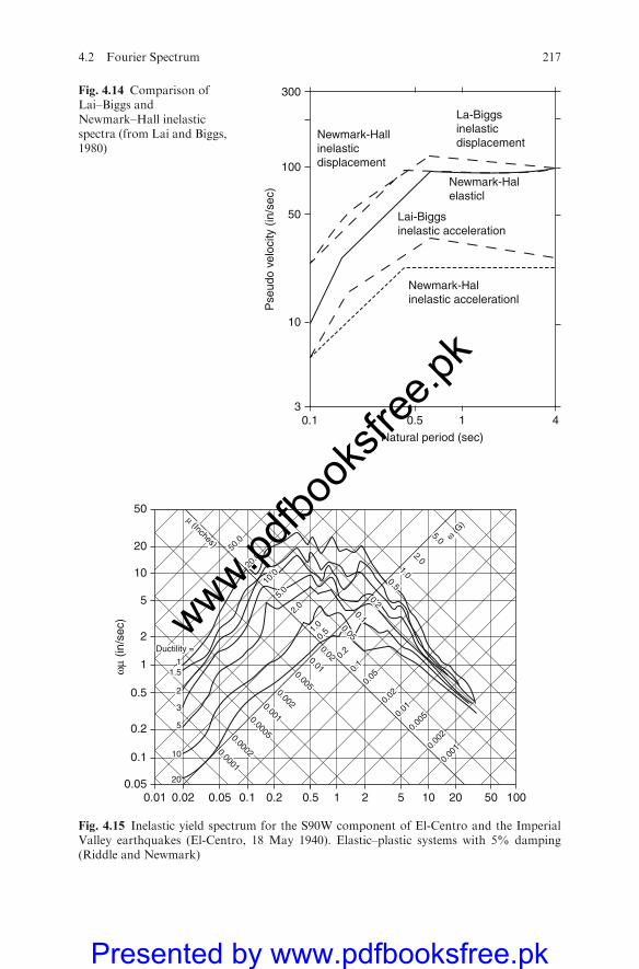
10
5
3
2
1.51
Ductility =
0.00010.
0010.
002
0.00
50.01
0.02
0.05
0.1
ωμ (G)
0.2
0.51.
0
2.0
5.0
10.0
20.0
50.0
0.0002
0.0005
0.001
0.002
0.005
0.01
μ (Inches)
0.02
0.05
0.1
0.2
0.5
1.0
2.0
5.0
20
10
5
3
2
1.51
Ductility =
0.010.05
0.1
0.2
0.5
1
2
5
10
20
50
0.02 0.05 0.1 0.2 0.5 1 2 5 10 20 50 100
0.00010.
0010.
002
0.00
50.01
0.02
0.05
0.1
ω (G)
0.2
0.51.
0
2.0
5.0
10.0
20.0
50.0
0.0002
0.0005
0.001
0.002
0.005
0.01
μ (Inches)
0.02
0.05
0.1
0.2
0.5
1.0
2.0
5.0
ωμ
(in/s
ec)
Fig. 4.15 Inelastic yield spectrum for the S90W component of El-Centro and the ImperialValley earthquakes (El-Centro, 18 May 1940). Elastic–plastic systems with 5% damping(Riddle and Newmark)
300
Pse
udo
velo
city
(in
/sec
)
100
50
10
30.1 0.5
Natural period (sec)
Newmark-Halinelastic accelerationl
Lai-Biggsinelastic acceleration
Newmark-Halelasticl
La-Biggsinelasticdisplacement
Newmark-Hallinelasticdisplacement
1 4
Fig. 4.14 Comparison ofLai–Biggs andNewmark–Hall inelasticspectra (from Lai and Biggs,1980)
4.2 Fourier Spectrum 217
www.pdfbo
oksfr
ee.pk
Presented by www.pdfbooksfree.pk
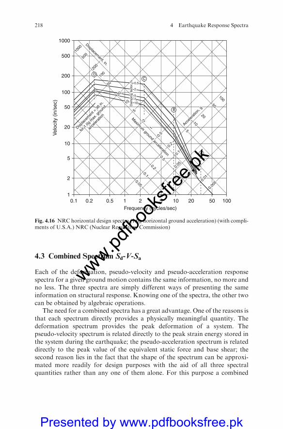
4.3 Combined Spectrum Sd-V-Sa
Each of the deformation, pseudo-velocity and pseudo-acceleration responsespectra for a given ground motion contains the same information, no more andno less. The three spectra are simply different ways of presenting the sameinformation on structural response. Knowing one of the spectra, the other twocan be obtained by algebraic operations.
The need for a combined spectra has a great advantage. One of the reasons isthat each spectrum directly provides a physically meaningful quantity. Thedeformation spectrum provides the peak deformation of a system. Thepseudo-velocity spectrum is related directly to the peak strain energy stored inthe system during the earthquake; the pseudo-acceleration spectrum is relateddirectly to the peak value of the equivalent static force and base shear; thesecond reason lies in the fact that the shape of the spectrum can be approxi-mated more readily for design purposes with the aid of all three spectralquantities rather than any one of them alone. For this purpose a combined
Displacement, in.
0.05
0.1
0.2
0.5
Maxim
um ground acceleration
0.00
50.
01
0.05
0.02
0.1
0.2
Accele
ratio
n, g
Displac
emen
t = 3
6 in.
for 1
.0g
max
. gro
und
acce
lerat
ion
0.5
1
2
5
10
20
50
100
200
500
5
10
20
50
100
1000
Dam
ping
fact
or, %
75
2
10
0.5
Displacement, in.
0.11
2
5
10
20
50
100
200
500
1000
0.2 0.5 1 2Frequency (cycles/sec)
Vel
ocity
(in
/sec
)
0.05
0.1
0.2
0.5
Maxim
um ground acceleration
0.00
50.
01
0.05
0.02
0.1
0.2
Accele
ratio
n, g
Displac
emen
t = 3
6 in.
for 1
.0g
max
. gro
und
acce
lerat
ion
0.5
1
2
5
10
20
50
100
200
500
5
10
20
50
100
5 10 20 50 100
A
B
CD
1000
Dam
ping
fact
or, %
75
2
10
0.5
Fig. 4.16 NRC horizontal design spectra (1.0g horizontal ground acceleration) (with compli-ments of U.S.A.) NRC (Nuclear Regulatory Commission)
218 4 Earthquake Response Spectra
www.pdfbo
oksfr
ee.pk
Presented by www.pdfbooksfree.pk
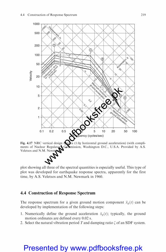
plot showing all three of the spectral quantities is especially useful. This type of
plot was developed for earthquake response spectra, apparently for the first
time, by A.S. Veletsos and N.M. Newmark in 1960.
4.4 Construction of Response Spectrum
The response spectrum for a given ground motion component €xgðtÞ can be
developed by implementation of the following steps:
1. Numerically define the ground acceleration €xgðtÞ; typically, the groundmotion ordinates are defined every 0.02 s.
2. Select the natural vibration period T and damping ratio z of an SDF system.
0.05
0.1
0.2
5
10
20
50
100
Maxim
um horizontal
ground acceleration
Maximum vertical
ground acceleration
Accele
ratio
n, g
Displacement, in.
5
10
20
50
100
200
500
1000
0.1
0.2
0.5
1
2
0.00
50.
010.
02
Dam
ping
fact
or, %
75
2
10
0.5
Displac
emen
t = 3
6 in.
for 1
.0g
max
. gro
und
acce
lerat
ion
0.1 0.2 0.5 1 2
Frequency (cycles/sec)
5 10 20 50 100
1
2
5
10
20
50
100
200
500
1000
Vel
ocity
Aα
B
C
D
0.05
0.1
0.2
5
10
20
50
100
Maxim
um horizontal
ground acceleration
Maximum vertical
ground acceleration
Accele
ratio
n, g
Displacement, in.
5
10
20
50
100
200
500
1000
0.1
0.2
0.5
1
2
0.00
50.
010.
02
Dam
ping
fact
or, %
75
2
10
0.5
Displac
emen
t = 3
6 in.
for 1
.0g
max
. gro
und
acce
lerat
ion
Fig. 4.17 NRC vertical design spectra (1.0g horizontal ground acceleration) (with compli-ments of Nuclear Regulatory Commission, Washington D.C., U.S.A. Provided by A.S.Veletsos and N.M. Newmark)
4.4 Construction of Response Spectrum 219
www.pdfbo
oksfr
ee.pk
Presented by www.pdfbooksfree.pk
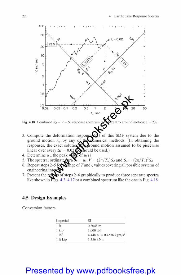
3. Compute the deformation response dðtÞ of this SDF system due to theground motion €xg by any of the numerical methods. (In obtaining theresponses, the exact solution for ground motion assumed to be piecewiselinear over every Dt ¼ 0:02 sec should be used.)
4. Determine uo, the peak value of u(t).5. The spectral ordinates are dd ¼ u0;V ¼ ð2p=TnÞSd and Sa ¼ ð2p=TnÞ2Sd
6. Repeat steps 2–5 for a range ofT and z values covering all possible systems ofengineering interest.
7. Present the results of steps 2–6 graphically to produce three separate spectralike shown in Figs. 4.3–4.17 or a combined spectrum like the one in Fig. 4.18.
4.5 Design Examples
Conversion factors
Imperial SI
1 ft 0.3048 m
1 kip 1,000 lbf
1 lbf 4.448 N ¼ 0.4536 kgm/s2
1 ft kip 1.356 kNm
0.020.2
0.5
1
2
5
10
20
50
100
0.05 0.1 0.2 0.5 1
Tn, sec
V, i
n./ s
ec
2 5 10
0.00
10.01
0.1
10
100
1
0.01
0.1
10
1
20 50
7.470.19
19
S d, in
.Sa, θ
23.5
ζ = 0.02
Fig. 4.18 Combined Sd � V� Sa response spectrum for El-Centro ground motion; z ¼ 2%
220 4 Earthquake Response Spectra
www.pdfbo
oksfr
ee.pk
Presented by www.pdfbooksfree.pk
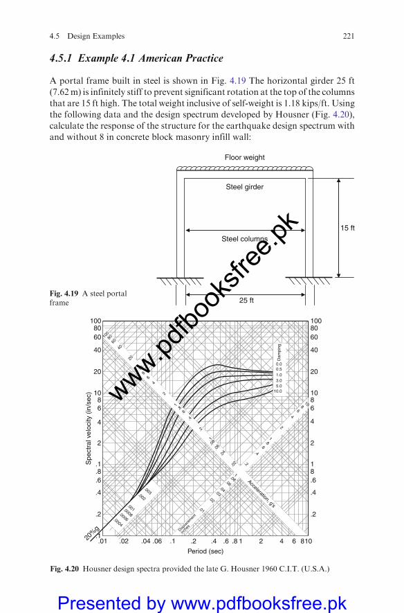
4.5.1 Example 4.1 American Practice
A portal frame built in steel is shown in Fig. 4.19 The horizontal girder 25 ft
(7.62m) is infinitely stiff to prevent significant rotation at the top of the columns
that are 15 ft high. The total weight inclusive of self-weight is 1.18 kips/ft. Using
the following data and the design spectrum developed by Housner (Fig. 4.20),
calculate the response of the structure for the earthquake design spectrum with
and without 8 in concrete block masonry infill wall:
Floor weight
Steel girder
Steel columns
25 ft
15 ft
Fig. 4.19 A steel portalframe
1008060
40
Dam
ping
20
10.05.03.01.00.50.0
1086
4
2
18.6
.4
Acceleration, g’s
.2
1086421.8.6.4
Period (sec)
.2
Displac
emen
t
inche
s
.1.06.04.02
.0004
.0006
.0008
.001
.002
.003
100
8060
40
20
108
64
2
1.8
.6.4
.2
.1.0
8.0
6.0
4
.02
.01
.02
.03
.04
.06
.08.1
.2
.4
.6.8
1
2
46
810
.0120%
g.1
.2
.4
.6
.8
2
Spe
ctra
l vel
ocity
(in
/sec
)
4
68
10
20
40
6080
100
.1
Fig. 4.20 Housner design spectra provided the late G. Housner 1960 C.I.T. (U.S.A.)
4.5 Design Examples 221
www.pdfbo
oksfr
ee.pk
Presented by www.pdfbooksfree.pk
Steel:
IðcolumnÞ ¼ 56:4 in2
ES ¼ 30� 106 lb=in2 ð200G N=m2Þ
Concrete block masonry:
Em ¼ 1,500kip=in2
Ev ¼ shear modulus of elasticity ¼ 0:4Em
Masonry weight ¼ 100lbf=ft2
Using the US code
K ¼ stiffness ¼ 212EI
h3
� �¼ 2ð12Þð30� 106Þð56:4Þ � 10�3
ð15� 12Þ3¼ 6:963kip=ft
on ¼ffiffiffiffiffiffiffiffiK
M
r¼
ffiffiffiffiffiffiffiffiffiffiffiffiffiffiffi6:963
1:18�25386
s¼ 9:55 rad=s
Tn ¼2pon¼ 0:658 � 0:66 s
Using 5% damping, from Housner’s spectrum, Sv= 10 in/s. Thus,
Sa ¼2pTn
� �Sv ¼ 95:24in=s2
Sd ¼Tn
2p
� �Sa ¼
0:66
2p
� �2
�95:24 ¼ 1:05 in
Sd is the relative displacement between the top and bottom of the column.Now
Seismic coefficient ¼ floor mass� acceleration
floor weight
¼ S a
g¼ 95:24
386� 0:25
The total shear force in the two columns at the ground level is equal to floormass � acceleration of the mass.
222 4 Earthquake Response Spectra
www.pdfbo
oksfr
ee.pk
Presented by www.pdfbooksfree.pk
Base shear
V ¼ 0:250� 1:18� 25 ¼ 7:375 kips
or
V ¼ KSd ¼ 6:963� 1:05 ¼ 7:31 kips
The difference between the two methods for the base shear is due to the
difference between Sa and the true floor acceleration.Force–deflection equation
DcP¼ h3
3EMIþ 1:2 h
AEvh ¼ 15 ft ¼ 180in
¼ 180ð Þ3
3� 1500� 7:62 300ð Þ3
12
þ 1:2� 180
7:62� 300ð Þ � 0:4� 1500
¼ 2:337� 10�4in=kip
K ¼ stiffness ¼ P
Dc¼ 1
2:337� 10�4¼ 4; 279 kip=in
One-half weight of the wall¼ 12� 15� 25� 100 lbf=ft2 � 10�3 ¼ 18:75 kips
KT ¼ total spring constant ¼ 6:963þ 4; 279 ¼ 4; 286 kip=in
Wtotal ¼ 1:18� 25þ 18:75 ¼ 48:25 kips
on ¼ffiffiffiffiffiffiffiffiffiffiK
M¼
r ffiffiffiffiffiffiffiffiffiffiffiffiffiffiffiffi4286
48:25386
¼
vuut185:17 rad=s
Tn ¼2p
185:17¼ 0:0339 � 0:034
V ¼ SaW ¼ 0:24� 48:25 ¼ 11:58 kips
Using Housner’s diagram (Fig. 4.20)
Tn ¼ 0:03
Sv ¼ 0:45 in=s
Sa ¼ 0:24 and Sd ¼ 0:0021in
4.5 Design Examples 223
www.pdfbo
oksfr
ee.pk
Presented by www.pdfbooksfree.pk
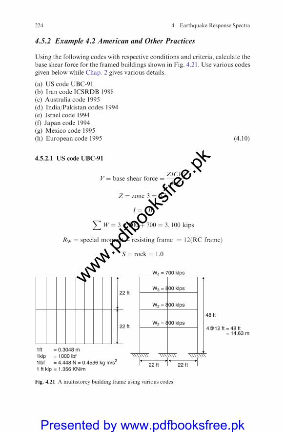
4.5.2 Example 4.2 American and Other Practices
Using the following codes with respective conditions and criteria, calculate thebase shear force for the framed buildings shown in Fig. 4.21. Use various codesgiven below while Chap. 2 gives various details.
(a) US code UBC-91(b) Iran code ICSRDB 1988(c) Australia code 1995(d) India/Pakistan codes 1994(e) Israel code 1994(f) Japan code 1994(g) Mexico code 1995(h) European code 1995 (4.10)
4.5.2.1 US code UBC-91
V ¼ base shear force ¼ ZICW
RW
Z ¼ zone 3 ¼ 0:3
I ¼ 1:0
XW ¼ 3� 800þ 700 ¼ 3; 100 kips
RW ¼ special moment � resisting frame ¼ 12ðRC frameÞ
S ¼ rock ¼ 1:0
22 ft
22 ft
1ft = 0.3048 m1klp = 1000 lbf1lbf = 4.448 N = 0.4536 kg m/s2
1 ft klp = 1.356 KN/m
W4 = 700 klps
W3 = 800 klps
W2 = 800 klps
W2 = 800 klps
48 ft
22 ft22 ft
4@12 ft = 48 ft= 14.63 m
Fig. 4.21 A multistorey building frame using various codes
224 4 Earthquake Response Spectra
www.pdfbo
oksfr
ee.pk
Presented by www.pdfbooksfree.pk
C ¼ 1:25S
T2=3Z
¼ 1:25� 1
0:03� ð48Þ3=4h i2=3 ¼ 1:25� 1:0
ð0:55Þ2=3¼ 1:862
V ¼ 0:3� 1:0� 1:862� 3100
12¼ 144:305 kipsð642 kNÞ
4.5.2.2 Iran Code ICSRDB 1988
TZ ¼ 0:07H3=4 ¼ 0:07� ð14:63Þ3=4 ¼ 0:524
HðmetresÞ ¼ 0:3048� 48 ¼ 14:63 m
T0 ¼ soil type 1 ¼ 0:3X
W ¼ 3,100 kips ¼ 3,100� 103 � 4:448
103¼ 13,789 kN
I ¼ important factor ¼ 1:0
R ¼ behaviour coefficient ¼ 7:0
A ¼ design base acceleration ¼ 0:35
B ¼ response coefficient ¼ 2T0
TZ
� �2=3
¼ 0:3
0:524
� �2=3
¼ 0:689
where 0:6 � B � 2:0
C ¼ seismic coefficient ¼ ABI
R¼ 0:35� 0:689� 1:0
7:0¼ 0:035
V ¼ base shear ¼ CW ¼ 0:035� 13,789 ¼ 475 kN
4.5.2.3 Australia Code 1995
V ¼ total seismic base shear ¼ ISC
RfGg
Gg ¼ 13; 789 kN
Vmin ¼ 0:01Gg ¼ 137:89 kN
Vmax ¼2:5Ia
RfGg ¼ 2:5� 1� 0:10
6� 13; 789 ¼ 575 kN
V ¼ 1� 0:25� 0:67
6� 13789 ¼ 386:5 kN
4.5 Design Examples 225
www.pdfbo
oksfr
ee.pk
Presented by www.pdfbooksfree.pk
where
a ¼ 0:10
I ¼ 1:0
S ðsoilÞ ¼ 0:67
R ¼ 6
Kd ¼ 5
C ¼ seismic design coefficient
¼ 1:25a
T2=3¼ 1:25� 0:10
ð0:252Þ2=3¼ 1:25� 0:10
0:498¼ 0:251
TZ ¼hn46¼ 48� 0:3048
46¼ 0:318 s
or
TZ ¼48� 0:3048
58¼ 0:252 s ðadopt this valueÞ
4.5.2.4 India/Pakistan Codes 1994
Total weight of the building frameP
W ¼ 13; 789 kN
bðsoilÞ ¼ 1:0
I ¼ ðimportance factorÞ ¼ 1:0
K = (performance factor) = 1.0
TZðinX� directionÞ ¼ 0:1n ¼ 0:1� 4 ¼ 0:4 s
TZðin y� directionÞ ¼ 0:09Hffiffiffidp ¼ 0:09� 14:63ffiffiffiffiffiffiffiffiffiffiffi
13:41p ¼ 0:36 sec
Adopt TZ ¼ 0:4 for maximum dimension, then C ¼ 0:9; a0 ¼ 0:08:
V ¼ base shear ¼ KCbIa0W
¼ 1� 0:9� 1� 0:08� 13789 ¼ 992:8 kN
226 4 Earthquake Response Spectra
www.pdfbo
oksfr
ee.pk
Presented by www.pdfbooksfree.pk
4.5.2.5 Israel Code 1994
TZðfor concrete frameÞ ¼ 0:073H3=4 ¼ 0:073 ð14:63Þ3=4 ¼ 0:546 s
XW ¼ 13; 789 kN
K ¼ reduction factor ¼ 5:5
I ¼ importance factor ¼ 1:0
Z ¼ acceleration factor ¼ 0:1
S (soil) = 1.2
RaðTnÞ ¼ spectral amplification factor
¼ 1:25S
T2=3Z
¼ 1:25� 1:2
ð0:546Þ2=3¼ 2:246
But
RaðTZÞ � 0:2K ¼ 0:2� 5:5 ¼ 1:152:246
Adopt RaðTZÞ ¼ 2:246
Cd ¼ seismic coefficient ¼ RaIZ
K¼ 2:246� 1� 0:1
5:5¼ 0:041
Cd �SIZffiffiffiffiffiffiffi3Kp ¼ 1:2� 1� 0:1ffiffiffiffiffiffiffiffiffiffiffiffiffiffiffi
3� 5:5p ¼ 0:0295 ðadoptedÞ
V ¼ base shear force
¼ Cd
XWi ¼ 0:0295� 13789 � 407 kN
On the basis of Cd ¼ 0:041
0:041
0:0295� 407 � 565 kN
4.5 Design Examples 227
www.pdfbo
oksfr
ee.pk
Presented by www.pdfbooksfree.pk
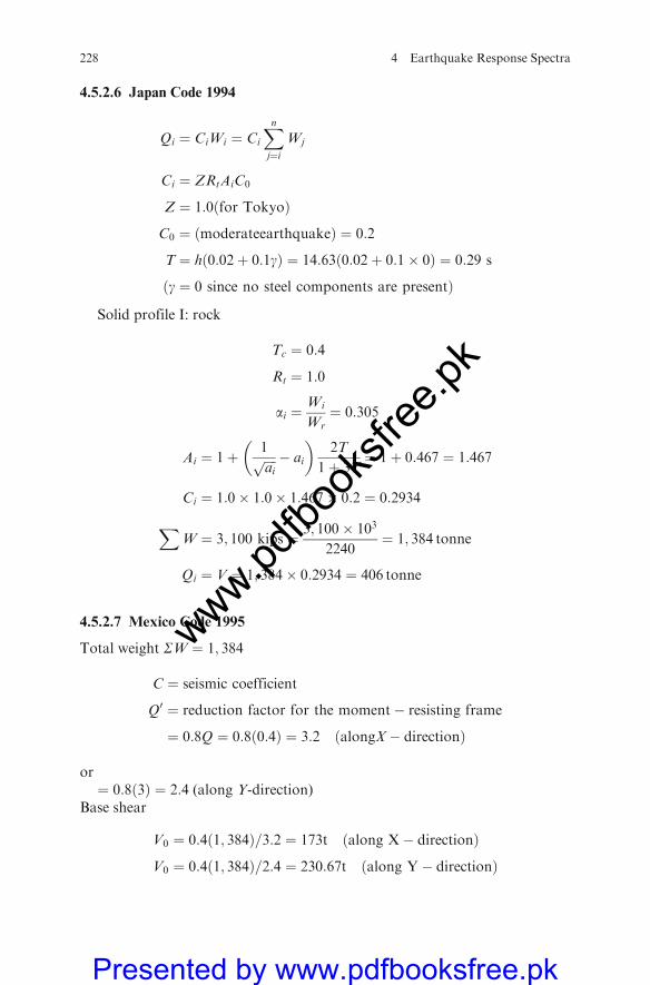
4.5.2.6 Japan Code 1994
Qi ¼ CiWi ¼ Ci
Xnj¼i
Wj
Ci ¼ ZRtAiC0
Z ¼ 1:0ðfor TokyoÞ
C0 ¼ ðmoderateearthquakeÞ ¼ 0:2
T ¼ hð0:02þ 0:1gÞ ¼ 14:63ð0:02þ 0:1� 0Þ ¼ 0:29 s
ðg ¼ 0 since no steel components are presentÞ
Solid profile I: rock
Tc ¼ 0:4
Rt ¼ 1:0
ai ¼Wi
Wr¼ 0:305
Ai ¼ 1þ 1ffiffiffiffiaip � ai
� �2T
1þ 3T¼ 1þ 0:467 ¼ 1:467
Ci ¼ 1:0� 1:0� 1:467� 0:2 ¼ 0:2934
XW ¼ 3; 100 kips ¼ 3; 100� 103
2240¼ 1; 384 tonne
Qi ¼ V ¼ 1; 384� 0:2934 ¼ 406 tonne
4.5.2.7 Mexico Code 1995
Total weight SW ¼ 1; 384
C ¼ seismic coefficient
Q0 ¼ reduction factor for the moment� resisting frame
¼ 0:8Q ¼ 0:8ð0:4Þ ¼ 3:2 ðalongX� directionÞ
or¼ 0:8ð3Þ ¼ 2:4 (along Y-direction)
Base shear
V0 ¼ 0:4ð1; 384Þ=3:2 ¼ 173t ðalong X� directionÞ
V0 ¼ 0:4ð1; 384Þ=2:4 ¼ 230:67t ðalong Y� directionÞ
228 4 Earthquake Response Spectra
www.pdfbo
oksfr
ee.pk
Presented by www.pdfbooksfree.pk
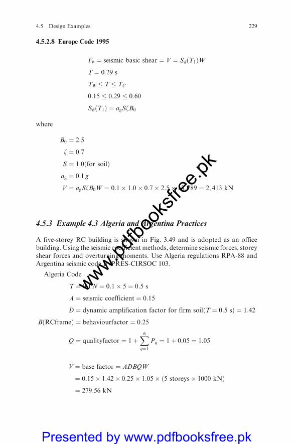
4.5.2.8 Europe Code 1995
Fb ¼ seismic basic shear ¼ V ¼ SdðT1ÞW
T ¼ 0:29 s
TB � T � TC
0:15 � 0:29 � 0:60
SdðT1Þ ¼ agSzB0
where
B0 ¼ 2:5
z ¼ 0:7
S ¼ 1:0ðfor soilÞ
ag ¼ 0:1 g
V ¼ agSzB0W ¼ 0:1� 1:0� 0:7� 2:5� 13; 789 ¼ 2; 413 kN
4.5.3 Example 4.3 Algeria and Argentina Practices
A five-storey RC building is shown in Fig. 3.49 and is adopted as an officebuilding. Using the seismic coefficient methods, determine seismic forces, storeyshear forces and overturning moments. Use Algeria regulations RPA-88 andArgentina seismic code INPRES-CIRSOC 103.
Algeria Code
T ¼ 0:1N ¼ 0:1� 5 ¼ 0:5 s
A ¼ seismic coefficient ¼ 0:15
D ¼ dynamic amplification factor for firm soilðT ¼ 0:5 sÞ ¼ 1:42
BðRCframeÞ ¼ behaviourfactor ¼ 0:25
Q ¼ qualityfactor ¼ 1þX6q¼1
Pq ¼ 1þ 0:05 ¼ 1:05
V ¼ base factor ¼ ADBQW
¼ 0:15� 1:42� 0:25� 1:05� ð5 storeys� 1000 kNÞ
¼ 279:56 kN
4.5 Design Examples 229
www.pdfbo
oksfr
ee.pk
Presented by www.pdfbooksfree.pk
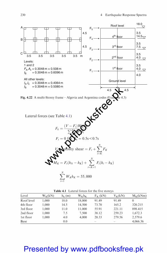
Lateral forces (see Table 4.1)
Fk ¼ðV� FtÞWKhKPN
i¼1 Wihi
Ft ¼ 0 for Tn ¼ 0:5s50:7s
Vk ¼ storey shear ¼ Ft þXNi¼K
FK
MK ¼ FtðhN � hKÞ þXNi¼Kþ1
Fiðhi � hKÞ
XNi¼1
WKhK ¼ 55; 000
Table 4.1 Lateral forces for the five storeys
Level WK(kN) hk (m) WKhK FK (kN) VK(kN) MK(kNm)
Roof level 1,000 18.0 18,000 91.49 91.49 0
4th floor 1,000 14.5 14,500 73.70 165.2 320.215
3rd floor 1,000 11.0 11,000 55.91 221.11 898.415
2nd floor 1,000 7.5 7,500 38.12 259.23 1,672.3
1st floor 1,000 4.0 4,000 20.33 279.56 2,579.6
Base 0.0 – – 4,066.36
18.0
3.514.5
3.57.5
3.54.0
3.54.0
4.0
4.5 4.5
Roof level
4th floor
3rd floor
2nd floor
1st floor
Ground level
F5
F4
F3
F2
F1
A
B
C3.5 3.5 3.5 3.5
4.5
4.5
3.5 m
Levels:1 and 2FA,Ac = 0.3048 m × 0.508 mIB = 0.3048 m × 0.6096 m
All other levels:IA,IC = 0.3048 m × 0.4064 mIB = 0.3048 m × 0.5080 m
Fig. 4.22 A multi-Storey frame – Algevia and Argentina codes (Example 4.3)
230 4 Earthquake Response Spectra
www.pdfbo
oksfr
ee.pk
Presented by www.pdfbooksfree.pk
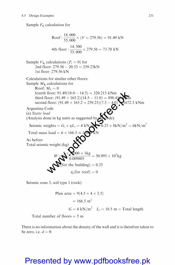
Sample FK calculation for
Roof :18; 000
55; 000� ðV ¼ 279:56Þ ¼ 91:49 kN
4th floor :14; 500
55; 000� 279:56 ¼ 73:70 kN
Sample VK calculations ðFt ¼ 0Þ for2nd floor: 279:56� 20:33 ¼ 259:23kN1st floor: 279.56 kN
Calculations for similar other floors:Sample MK calculations for
Roof: Mk ¼ 0fourth floor: 91:49ð18:0� 14:5Þ ¼ 320:215 kNmthird floor: ð91:49þ 165:2Þð14:5� 11:0Þ ¼ 898:415 kNmsecond floor: ð91:49þ 165:2þ 259:23Þð7:5� 4:0Þ ¼ 1672:3 kNm
Argentina Code(a) Static load(Analysis done in kg units as suggested by the code):
Seismic weights ¼ Gi þ ZLi ¼ 4 kN=m2 þ 0:25� 8kN=m2 ¼ 6kN=m2
Total mass load ¼ 6� 166:5 � 1; 000 kN
As beforeTotal seismic weight (kg)
W ¼ 5� 1; 000� 1kg
0:009805¼ 50:995� 105kg
Ziðfor the buildingÞ ¼ 0:25
Ziðfor roofÞ ¼ 0
Seismic zone 3, soil type 1 (rock)
Plan area ¼ 9ð4:5þ 4� 3:5Þ
¼ 166:5 m2
G ¼ 4 kN=m2 Li ¼ 18:5 m ¼ Total length
Total number of floors ¼ 5 m
There is no information about the density of the wall and it is therefore taken to
be zero, i.e. d ¼ 0:
4.5 Design Examples 231
www.pdfbo
oksfr
ee.pk
Presented by www.pdfbooksfree.pk
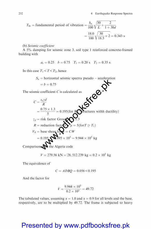
T0e ¼ fundamental period of vibration ¼ hn100
ffiffiffiffiffiffiffiffiffiffiffiffiffiffiffiffiffiffiffiffiffiffiffiffiffiffiffi30
Lþ 2
1þ 30d
r
¼ 18:0
100
ffiffiffiffiffiffiffiffiffiffiffiffiffiffiffiffiffi30
18:5þ 2
r¼ 0:343 s
(b) Seismic coefficientA 5% damping for seismic zone 3, soil type 1 reinforced concrete-framed
building with
as ¼ 0:25 b ¼ 0:75 T1 ¼ 0:20 s T2 ¼ 0:35 s
In this case T15T5T2, hence
Sa ¼ horizontal seismic spectra pseudo� acceleration
¼ b ¼ 0:75
The seismic coefficient C is calculated as
C ¼ sagdR
¼ 0:75� 1:3
5¼ 0:195ðfor RC structures withh ductilityÞ
gd ¼ risk factor Group A ¼ 1:3
R ¼ reduction factors ¼ m ¼ 5ðforT � T1Þ
V0 ¼ base shear force ¼ CW
¼ 0:195� 50:995� 105 ¼ 9:944� 105 kg
Comparison with the Algeria code
V ¼ 279:56 kN ¼ 28; 512:239 kg ¼ 0:2� 105 kg
The equivalence of
C ¼ ADBQ ¼ 0:05650:195
And the factor for
V ¼ 9:944� 105
0:2� 105¼ 49:72
The tabulated values, assuming a ¼ 1:0 and a ¼ 0:9 for all levels and the base,respectively, are to be multiplied by 49.72. The frame is subjected to heavy
232 4 Earthquake Response Spectra
www.pdfbo
oksfr
ee.pk
Presented by www.pdfbooksfree.pk

lateral loads and overturning moments and this building in Argentina will haveto have a more robust design.
(c) Torsional momentTable 4.1 is extended to include torsional moments. A column is created in
Table 4.1 on the basis of
Mti ¼ ð1:5e1 þ 0:10LÞVi
¼ 0:1LVi
¼ 0:1� 18:5Vi
¼ 1:85Vi
e1 ¼ distance from the CS at level i and the line of action of the shear forcemeasured perpendicularly, assumed to be zero
all units in MKS, i.e. kg units.The modified V column � 1.85 will give the Mti values.
(d) Storey drifts, lateral displacement and storey distortions
Ki ¼ stiffness at ith level ¼ 12EIi=H3i
Hi ¼ 3:5 m storey height
Ec ¼ 2:1� 109kg=m2
Ii ¼ cross� sectional area moment of inertia for the storey column
(e) Storey drift Di
Given by
D ¼ mVi
Ki
Level Vi � 104 kg
Roof 0.9331
Fourth floor 1.8649
Third floor 2.2551
Second floor 2.6439
First floor 2.8512
Base –
(f) I for columns
For floors 1 and 2:
IA ¼ IC ¼1
12� 0:3048ð0:508Þ3 ¼ 3:3298� 10�3m4
IB ¼1
12� 0:3048ð0:6096Þ3 ¼ 5:7539� 10�3m4
4.5 Design Examples 233
www.pdfbo
oksfr
ee.pk
Presented by www.pdfbooksfree.pk
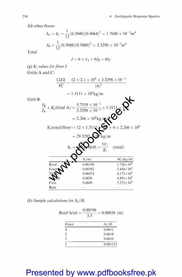
All other floors
IA ¼ IC ¼1
12ð0:3048Þð0:4064Þ3 ¼ 1:7048� 10�3m4
IB ¼1
12ð0:3048Þð0:5080Þ3 ¼ 3:3298� 10�3m4
Total
I ¼ 6� IA þ 6IB þ 6IC
(g) Ki values for floor I
Grids A and C:
12EIi
H3i
¼ 12� 2:1� 109 � 3:3298� 10�3
ð4Þ3
¼ 1:3111� 106kg=m
Grid B:
IBIA� KiðGrid AÞ ¼ 5:7539� 10�3
3:3298� 10�3� 1:3111� 106
¼ 2:266� 106kg=m
KiðtotalÞfloor ¼ 12� 1:3111� 106 þ 6� 2:266� 106
¼ 29:3292� 106kg=m
Di ¼ storey drift ¼ 5Vi
KiðtotalÞ
DiðmÞ Mtiðkg=mÞRoof 0.00196 1.726�104Fourth 0.00392 3.450�104Third 0.00474 4.172�104Second 0.0056 4.891�104First 0.0049 5.275�104Base – –
(h) Sample calculations for Di=Hi
Roof level ¼ 0:00196
3:5¼ 0:00056 ðmÞ
Floor Di=Hi
4 0.0011
3 0.0014
2 0.0016
1 0.001123
234 4 Earthquake Response Spectra
www.pdfbo
oksfr
ee.pk
Presented by www.pdfbooksfree.pk
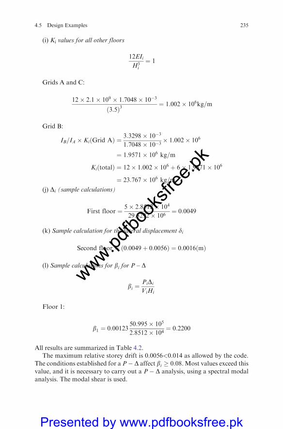
(i) Ki values for all other floors
12EIi
H3i
¼ 1
Grids A and C:
12� 2:1� 109 � 1:7048� 10�3
ð3:5Þ3¼ 1:002� 106kg=m
Grid B:
IB=IA � KiðGrid AÞ ¼ 3:3298� 10�3
1:7048� 10�3� 1:002� 106
¼ 1:9571� 106 kg=m
KiðtotalÞ ¼ 12� 1:002� 106 þ 6� 1:9571� 106
¼ 23:767� 106 kg=m
(j) Di (sample calculations)
First floor ¼ 5� 2:8512� 104
29:3292� 106¼ 0:0049
(k) Sample calculation for the lateral displacement di
Second floor ¼ ð0:0049þ 0:0056Þ ¼ 0:0016ðmÞ
(l) Sample calculations for bi for P – D
bi ¼PiDi
ViHi
Floor 1:
b1 ¼ 0:0012350:995� 105
2:8512� 104¼ 0:2200
All results are summarized in Table 4.2.The maximum relative storey drift is 0.0056<0.014 as allowed by the code.
The conditions established for a P� D affect bi � 0:08. Most values exceed this
value, and it is necessary to carry out a P� D analysis, using a spectral modal
analysis. The modal shear is used.
4.5 Design Examples 235
www.pdfbo
oksfr
ee.pk
Presented by www.pdfbooksfree.pk
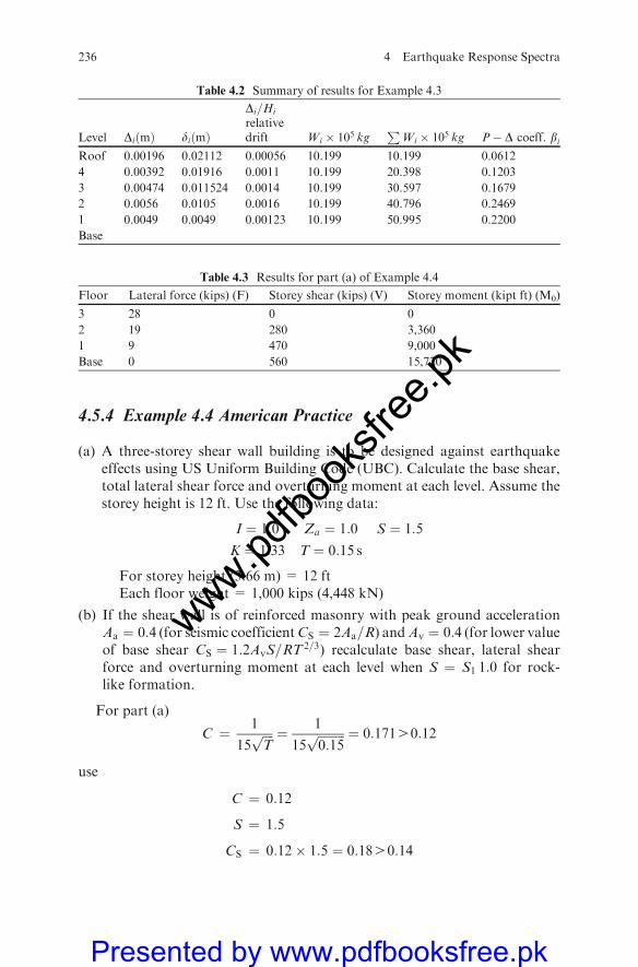
4.5.4 Example 4.4 American Practice
(a) A three-storey shear wall building is to be designed against earthquakeeffects using US Uniform Building Code (UBC). Calculate the base shear,total lateral shear force and overturning moment at each level. Assume thestorey height is 12 ft. Use the following data:
I ¼ 1:0 Za ¼ 1:0 S ¼ 1:5
K ¼ 1:33 T ¼ 0:15 s
For storey height (3.66 m) = 12 ftEach floor weight = 1,000 kips (4,448 kN)
(b) If the shear wall is of reinforced masonry with peak ground accelerationAa ¼ 0:4 (for seismic coefficientCS ¼ 2Aa=R) andAn ¼ 0:4 (for lower valueof base shear CS ¼ 1:2AnS=RT
2=3) recalculate base shear, lateral shearforce and overturning moment at each level when S ¼ S1 1:0 for rock-like formation.
For part (a)
C ¼ 1
15ffiffiffiffiTp ¼ 1
15ffiffiffiffiffiffiffiffiffi0:15p ¼ 0:17140:12
use
C ¼ 0:12
S ¼ 1:5
CS ¼ 0:12� 1:5 ¼ 0:1840:14
Table 4.2 Summary of results for Example 4.3
Level DiðmÞ diðmÞ
Di=Hi
relativedrift Wi � 105 kg
PWi � 105 kg P� D coeff: bi
Roof 0.00196 0.02112 0.00056 10.199 10.199 0.0612
4 0.00392 0.01916 0.0011 10.199 20.398 0.1203
3 0.00474 0.011524 0.0014 10.199 30.597 0.1679
2 0.0056 0.0105 0.0016 10.199 40.796 0.2469
1 0.0049 0.0049 0.00123 10.199 50.995 0.2200
Base
Table 4.3 Results for part (a) of Example 4.4
Floor Lateral force (kips) (F) Storey shear (kips) (V) Storey moment (kipt ft) (M0)
3 28 0 0
2 19 280 3,360
1 9 470 9,000
Base 0 560 15,720
236 4 Earthquake Response Spectra
www.pdfbo
oksfr
ee.pk
Presented by www.pdfbooksfree.pk
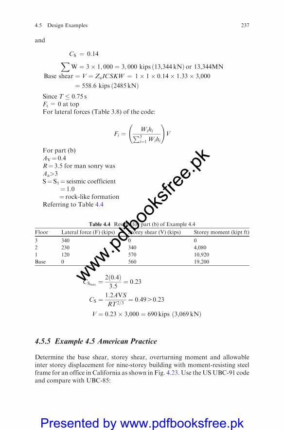
and
CS ¼ 0:14XW ¼ 3� 1; 000 ¼ 3; 000 kips 13,344 kNð Þ or 13,344MN
Base shear ¼ V ¼ ZaICSKW ¼ 1� 1� 0:14� 1:33� 3,000
¼ 558:6 kips 2485 kNð ÞSince T � 0:75 sFt = 0 at topFor lateral forces (Table 3.8) of the code:
Fi ¼WihiP3i¼1 Wihi
!V
For part (b)AV¼ 0.4R¼ 3.5 for man sonry wasAa>3S¼ S1¼ seismic coefficient
¼ 1.0¼ rock-like formation
Referring to Table 4.4
CSmax¼ 2 0:4ð Þ
3:5¼ 0:23
CS ¼1:2AVS
RT 2=3¼ 0:4940:23
V ¼ 0:23� 3,000 ¼ 690 kips 3,069 kNð Þ
4.5.5 Example 4.5 American Practice
Determine the base shear, storey shear, overturning moment and allowableinter storey displacement for nine-storey building with moment-resisting steelframe for an office in California as shown in Fig. 4.23. Use theUSUBC-91 codeand compare with UBC-85:
Table 4.4 Results for part (b) of Example 4.4
Floor Lateral force (F) (kips) Storey shear (V) (kips) Storey moment (kipt ft)
3 340 0 0
2 230 340 4,080
1 120 570 10,920
Base 0 560 19,200
4.5 Design Examples 237
www.pdfbo
oksfr
ee.pk
Presented by www.pdfbooksfree.pk

Data
Storey height = 13 ft = hx
Total load = 0.1 kip/ft2 (all levels)
Soil profile type 2, i.e. S2=1.2
Seismic coefficient C ¼ 115ffiffiffiTp or C ¼ 1:25S
T 2=3
Ductile moment frame and zone location: zone 4:
Base shear V ¼ ZaIKCSW or ZICWRW
RW ¼ 12
For zone 4:
Za ¼ 1
I = importance factor =1.0 (for the office building)K = ductile value =0.67
117 ft
Elevation
Plan
100 ft
170 ft
Fig. 4.23 Moment-resistingsteel-framed building
238 4 Earthquake Response Spectra
www.pdfbo
oksfr
ee.pk
Presented by www.pdfbooksfree.pk
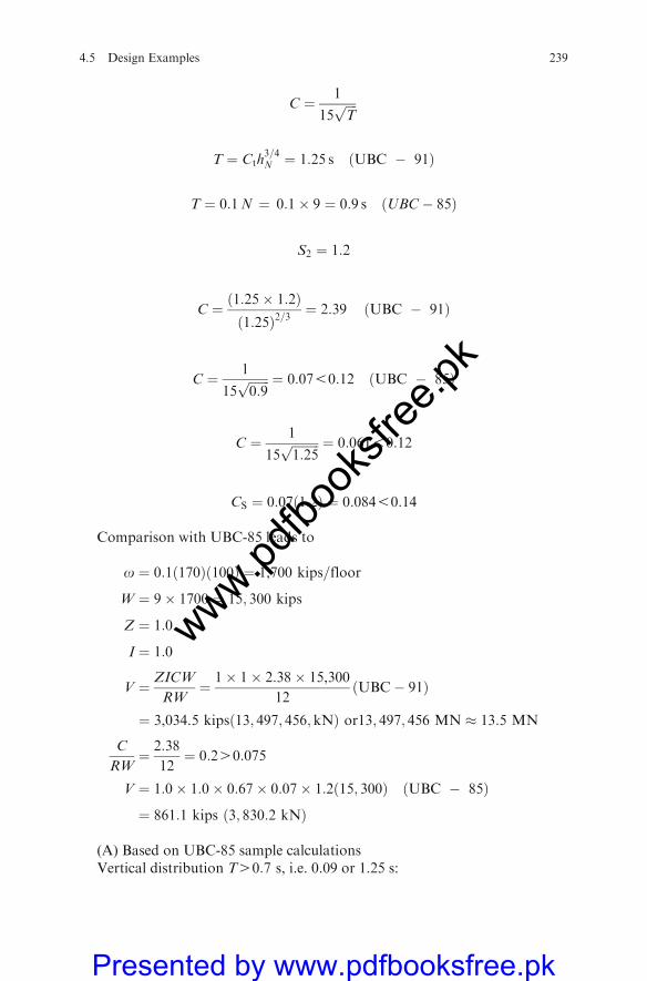
C ¼ 1
15ffiffiffiffiTp
T ¼ Cth3=4N ¼ 1:25 s UBC � 91ð Þ
T ¼ 0:1N ¼ 0:1� 9 ¼ 0:9 s UBC� 85ð Þ
S2 ¼ 1:2
C ¼ 1:25� 1:2ð Þ1:25ð Þ2=3
¼ 2:39 UBC � 91ð Þ
C ¼ 1
15ffiffiffiffiffiffiffi0:9p ¼ 0:0750:12 UBC � 85ð Þ
C ¼ 1
15ffiffiffiffiffiffiffiffiffi1:25p ¼ 0:06150:12
CS ¼ 0:07 1:2ð Þ ¼ 0:08450:14
Comparison with UBC-85 leads to
o ¼ 0:1ð170Þð100Þ ¼ 1,700 kips=floor
W ¼ 9� 1700 ¼ 15; 300 kips
Z ¼ 1:0
I ¼ 1:0
V ¼ ZICW
RW¼ 1� 1� 2:38� 15,300
12UBC� 91ð Þ
¼ 3,034.5 kips 13; 497; 456;kNð Þ or13; 497; 456 MN � 13:5 MN
C
RW¼ 2:38
12¼ 0:240:075
V ¼ 1:0� 1:0� 0:67� 0:07� 1:2 15; 300ð Þ UBC � 85ð Þ
¼ 861:1 kips 3; 830:2 kNð Þ
(A) Based on UBC-85 sample calculationsVertical distribution T40:7 s, i.e. 0.09 or 1.25 s:
4.5 Design Examples 239
www.pdfbo
oksfr
ee.pk
Presented by www.pdfbooksfree.pk
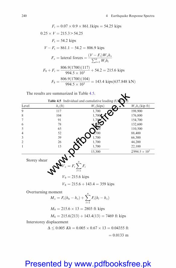
Ft ¼ 0:07� 0:9� 861:1kips ¼ 54:25 kips
0:25� V ¼ 215:3454:25
Ft ¼ 54:2 kips
V� Ft ¼ 861:1� 54:2 ¼ 806:9 kips
Fx ¼ lateral forces ¼ V� Ftð ÞWxhxPni¼1 Wihi
F9 þ Ft ¼806:9 1700ð Þ 117ð Þ
994:5� 103þ 54:2 ¼ 215:6 kips
F8 ¼806:9 1700ð Þ 104ð Þ
994:5� 103¼ 143:4 kips 637:848 kNð Þ
The results are summarized in Table 4.5.
Storey shear
Vx ¼ Ft
Xni¼x
Fi
V9 ¼ 215:6 kips
V8 ¼ 215:6þ 143:4 ¼ 359 kips
Overturning moment
Mx ¼ Ftðhn � hxÞ þXni¼1
Fiðhi � hxÞ
M9 ¼ 215:6� 13 ¼ 2803 ft kips
M8 ¼ 215:6ð213Þ þ 143:4ð13Þ ¼ 7469 ft kips
Interstorey displacement
D � 0:005 Kh ¼ 0:005� 0:67� 13 ¼ 0:04355 ft
¼ 0:0133 m
Table 4.5 Individual and cumulative loading (UBC-85)
Level hxðftÞ WxðkipsÞ Wxhxðkip ftÞ9 117 1,700 198,900
8 104 1,700 176,800
7 91 1,700 154,700
6 78 1,700 132,600
5 65 1,700 110,500
4 52 1,700 88,400
3 39 1,700 66,300
2 26 1,700 44,200
1 13 1,700 22,100
15,300 S994:5� 103
240 4 Earthquake Response Spectra
www.pdfbo
oksfr
ee.pk
Presented by www.pdfbooksfree.pk
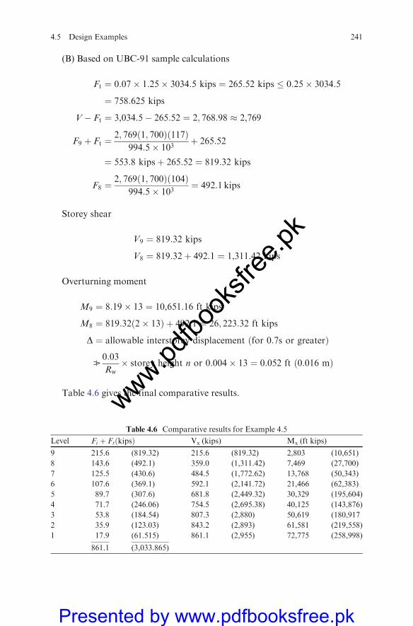
(B) Based on UBC-91 sample calculations
Ft ¼ 0:07� 1:25� 3034:5 kips ¼ 265:52 kips � 0:25� 3034:5
¼ 758:625 kips
V� Ft ¼ 3,034.5� 265:52 ¼ 2; 768:98 � 2,769
F9 þ Ft ¼2; 769ð1; 700Þð117Þ
994:5� 103þ 265:52
¼ 553:8 kipsþ 265:52 ¼ 819:32 kips
F8 ¼2; 769ð1; 700Þð104Þ
994:5� 103¼ 492:1 kips
Storey shear
V9 ¼ 819:32 kips
V8 ¼ 819:32þ 492:1 ¼ 1,311.42 kips
Overturning moment
M9 ¼ 8:19� 13 ¼ 10,651.16 ft kips
M8 ¼ 819:32ð2� 13Þ þ 492:1 ¼ 26; 223:32 ft kips
D ¼ allowable interstorey displacement ðfor 0:7s or greaterÞ
B0:03
Rw� storey height n or 0:004� 13 ¼ 0:052 ft ð0:016 mÞ
Table 4.6 gives the final comparative results.
Table 4.6 Comparative results for Example 4.5
Level Fi þ FtðkipsÞ Vx (kips) Mx (ft kips)
9 215.6 (819.32) 215.6 (819.32) 2,803 (10,651)
8 143.6 (492.1) 359.0 (1,311.42) 7,469 (27,700)
7 125.5 (430.6) 484.5 (1,772.62) 13,768 (50,343)
6 107.6 (369.1) 592.1 (2,141.72) 21,466 (62,383)
5 89.7 (307.6) 681.8 (2,449.32) 30,329 (195,604)
4 71.7 (246.06) 754.5 (2,695.38) 40,125 (143,876)
3 53.8 (184.54) 807.3 (2,880) 50,619 (180,917
2 35.9 (123.03) 843.2 (2,893) 61,581 (219,558)
1 17.9 (61.515) 861.1 (2,955) 72,775 (258,998)
861.1 (3,033.865)
4.5 Design Examples 241
www.pdfbo
oksfr
ee.pk
Presented by www.pdfbooksfree.pk
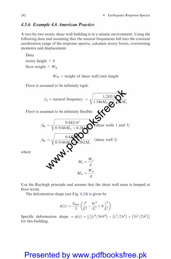
4.5.6 Example 4.6 American Practice
A two-by-two storey shear wall building is in a seismic environment. Using thefollowing data and assuming that the natural frequencies fall into the constantacceleration range of the response spectra, calculate storey forces, overturningmoments and displacement.
Data
storey height = h
floor weight = WS
WW ¼ weight of shear wall=unit length
Floor is assumed to be infinitely rigid:
fA ¼ natural frequency ¼
ffiffiffiffiffiffiffiffiffiffiffiffiffiffiffiffiffiffiffiffiffiffiffiffiffiffiffiffiffiffiffiffiffiffiffiffiffiffiffiffiffiffi1:2EI=h3
1:54hMw þ 1:125Ms
s
Floor is assumed to be infinitely flexible:
fB1¼
ffiffiffiffiffiffiffiffiffiffiffiffiffiffiffiffiffiffiffiffiffiffiffiffiffiffiffiffiffiffiffiffiffiffiffiffiffiffiffiffiffiffiffiffi0:4EI=h3
0:514hMw þ 0:281Ms
sðshear walls 1 and 3Þ
fB2¼
ffiffiffiffiffiffiffiffiffiffiffiffiffiffiffiffiffiffiffiffiffiffiffiffiffiffiffiffiffiffiffiffiffiffiffiffiffiffiffiffiffiffiffiffi0:4EI=h3
0:514hMw þ 0:562Ms
sðshear wall 2Þ
where
Ms ¼Ws
g
Mw ¼Ww
g
Use the Rayleigh principle and assume that the shear wall mass is lumped atfloor levels.
The deformation shape (see Fig. 4.24) is given by
fðzÞ ¼ dmax
3
z4
L4� 4z3
L3þ 6
z2
L2
� �
Specific deformation shape ¼ fðzÞ ¼ 13
z4=16 h4� �
� z3=2 h3� �
þ 3z2=2 h2� ��
for this building.
242 4 Earthquake Response Spectra
www.pdfbo
oksfr
ee.pk
Presented by www.pdfbooksfree.pk
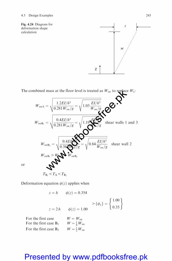
The combined mass at the floor level is treated as Wsw to replace Ws:
WswA ¼
ffiffiffiffiffiffiffiffiffiffiffiffiffiffiffiffiffiffiffiffiffiffiffiffiffiffiffiffiffiffiffiffiffiffiffiffiffiffiffiffiffiffiffiffiffiffiffiffiffiffiffiffiffiffiffiffiffiffiffi1:2EI=h3
0:281Wsw=g¼
ffiffiffiffiffiffiffiffiffiffiffiffiffiffiffiffiffiffiffiffiffiffiffi1:03
EI=h3
Wsw=g
svuut
WswB1¼
ffiffiffiffiffiffiffiffiffiffiffiffiffiffiffiffiffiffiffiffiffiffiffiffiffiffiffiffiffiffiffiffiffiffiffiffiffiffiffiffiffiffiffiffiffiffiffiffiffiffiffiffiffiffiffiffiffiffiffi0:4EI=h3
0:281Wsw=g¼
ffiffiffiffiffiffiffiffiffiffiffiffiffiffiffiffiffiffiffiffiffiffiffi1:19
EI=h3
Wsw=g
svuut shear walls 1 and 3
WswB2¼
ffiffiffiffiffiffiffiffiffiffiffiffiffiffiffiffiffiffiffiffiffiffiffiffiffiffiffiffiffiffiffiffiffiffiffiffiffiffiffiffiffiffiffiffiffiffiffiffiffiffiffiffiffiffiffiffiffiffiffi0:4EI=h3
0:562Wsw=g¼
ffiffiffiffiffiffiffiffiffiffiffiffiffiffiffiffiffiffiffiffiffiffiffi0:84
EI=h3
Wsw=g
svuut shear wall 2
WswB14WswA4WswB2
or
TB15TA5TB2
Deformation equation fðzÞ applies when
z ¼ h fðzÞ ¼ 0:354
z ¼ 2 h fðzÞ ¼ 1:00
4ff1g ¼1:00
0:35
( )
For the first case W ¼Wsw
For the first case B1 W ¼ 14Wsw
For the first case B2 W ¼ 12Wsw
δ
H
Z
Fig. 4.24 Diagram fordeformation shapecalculation
4.5 Design Examples 243
www.pdfbo
oksfr
ee.pk
Presented by www.pdfbooksfree.pk
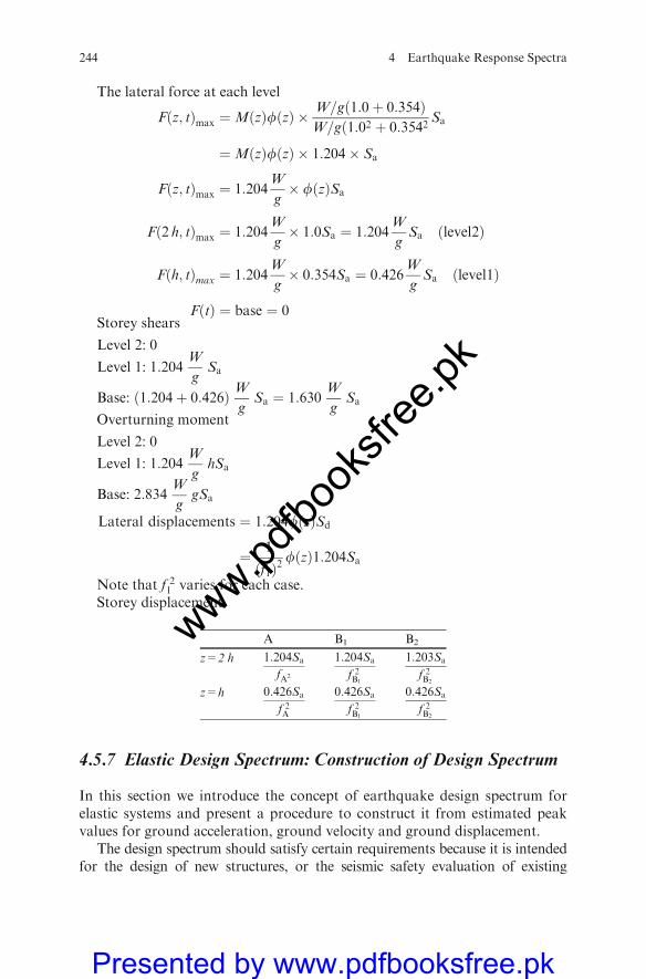
The lateral force at each level
Fðz; tÞmax ¼MðzÞfðzÞ � W=gð1:0þ 0:354ÞW=gð1:02 þ 0:3542
Sa
¼MðzÞfðzÞ � 1:204� Sa
Fðz; tÞmax ¼ 1:204W
g� fðzÞSa
Fð2 h; tÞmax ¼ 1:204W
g� 1:0Sa ¼ 1:204
W
gSa ðlevel2Þ
Fðh; tÞmax ¼ 1:204W
g� 0:354Sa ¼ 0:426
W
gSa ðlevel1Þ
FðtÞ ¼ base ¼ 0Storey shears
Level 2: 0
Level 1: 1:204W
gSa
Base: ð1:204þ 0:426Þ Wg
Sa ¼ 1:630W
gSa
Overturning moment
Level 2: 0
Level 1: 1:204W
ghSa
Base: 2:834W
ggSa
Lateral displacements ¼ 1:204fðzÞSd
¼ 1
ðf1Þ2fðzÞ1:204Sa
Note that f 21 varies for each case.
Storey displacement
A B1 B2
z=2 h 1:204Sa
fA2
1:204Sa
f 2B1
1:203Sa
f 2B2
z=h 0:426Sa
f 2A
0:426Sa
f 2B1
0:426Sa
f 2B2
4.5.7 Elastic Design Spectrum: Construction of Design Spectrum
In this section we introduce the concept of earthquake design spectrum forelastic systems and present a procedure to construct it from estimated peakvalues for ground acceleration, ground velocity and ground displacement.
The design spectrum should satisfy certain requirements because it is intendedfor the design of new structures, or the seismic safety evaluation of existing
244 4 Earthquake Response Spectra
www.pdfbo
oksfr
ee.pk
Presented by www.pdfbooksfree.pk
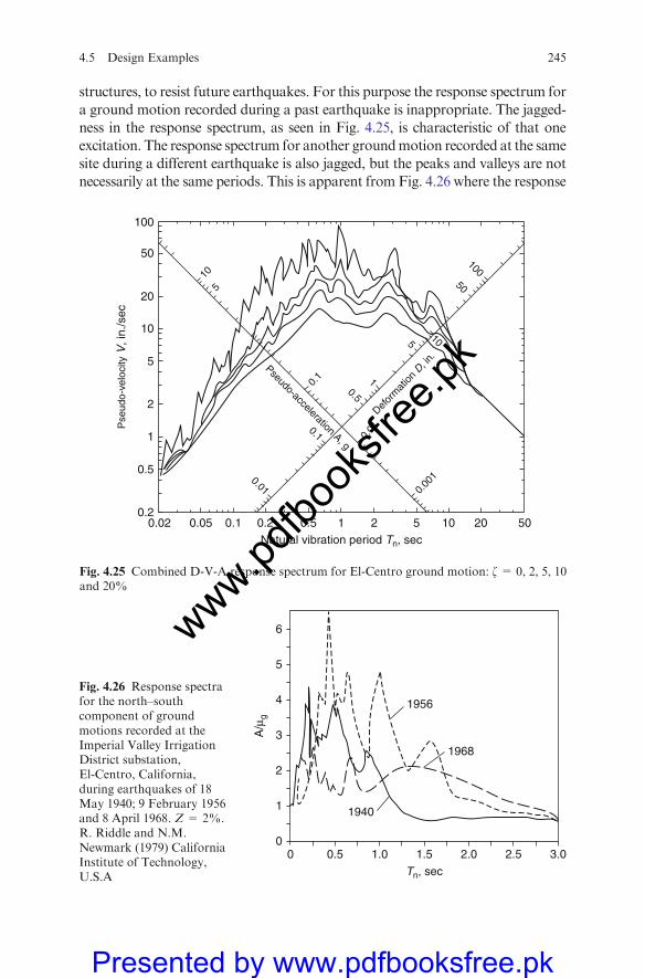
structures, to resist future earthquakes. For this purpose the response spectrum for
a ground motion recorded during a past earthquake is inappropriate. The jagged-
ness in the response spectrum, as seen in Fig. 4.25, is characteristic of that one
excitation. The response spectrum for another groundmotion recorded at the same
site during a different earthquake is also jagged, but the peaks and valleys are not
necessarily at the same periods. This is apparent from Fig. 4.26 where the response
0.050.020.2
0.5
1
2
5
10
20
50
100
0.1 0.2 0.5Natural vibration period Tn, sec
Pse
udo-
velo
city
V, i
n./s
ec
1 2 5 10 20 50
0.00
10.01
0.1
0.5
Pseudo-acceleration A, g
1
5
50
100
10
0.01
Deform
ation
D, in
.
0.1
510
Fig. 4.25 Combined D-V-A response spectrum for El-Centro ground motion: z = 0, 2, 5, 10and 20%
00
1
3
2
4
5
6
0.5 1.0 1.5
1940
1968
1956
2.52.0 3.0
A/μ
g
Tn, sec
Fig. 4.26 Response spectrafor the north–southcomponent of groundmotions recorded at theImperial Valley IrrigationDistrict substation,El-Centro, California,during earthquakes of 18May 1940; 9 February 1956and 8 April 1968. Z = 2%.R. Riddle and N.M.Newmark (1979) CaliforniaInstitute of Technology,U.S.A
4.5 Design Examples 245
www.pdfbo
oksfr
ee.pk
Presented by www.pdfbooksfree.pk
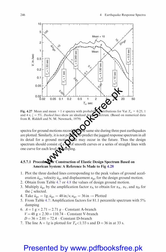
spectra for groundmotions recorded at the same site during three past earthquakesare plotted. Similarly, it is not possible to predict the jagged response spectrum in allits detail for a ground motion that may occur in the future. Thus the designspectrum should consist of a set of smooth curves or a series of straight lines withone curve for each level of damping.
4.5.7.1 Procedure for Construction of Elastic Design Spectrum Based on
American System: A Reference Is Made to Fig 4.28
1. Plot the three dashed lines corresponding to the peak values of ground accel-eration €ugo, velocity _ugo and displacement ugo for the design ground motion.
2. Obtain from Table 4.7 or 4.8 the values of design ground motion.3. Multiply €ugo by the amplification factor aA to obtain for aA; aV, and aD for
the z selected.4. Take €ugo ¼ 1g; _ugo ¼ 48 in=s; ugo ¼ 36 in! Plotted5. From Table 4.7: Amplification factors for 81.1 percentile spectrum with 5%
damping6. A¼ 1 g� 2.71¼ 2.71 g – Constant A-branch
V¼ 48 g� 2.30¼ 110.74 – Constant V-branchD¼ 36� 2.01¼ 72.4 – Constant D-branch
7. The line A¼ 1g is plotted for Tn<1/33 s and D¼ 36 in at 33 s.
0.020.02
0.05
0.1
0.2
0.5
1
2
5
10
0.05 0.1 0.2 0.5 1 2 5 10 20 50Tn, sec
V, i
n./s
ec
Mean
Mean + 10
Tu
= 1
sec
Te
= 1
0 se
c
Ts
= 0
.3 s
ec
Tu
= 1
.53
sec
A/ugo
D/u go
0.01
0.001
0.01
0.1
1
10
0.1
1
10
100
d
Td
= 3
.130
sec
Tc
= 0
.349
sec
Fig. 4.27 Mean and mean +1 s spectra with probability distributions for Vat Tn = 0.25, 1and 4 s; z ¼ 5%. Dashed lines show an idealized design spectrum. (Based on numerical datafrom R. Riddell and N. M. Newmark, 1979)
246 4 Earthquake Response Spectra
www.pdfbo
oksfr
ee.pk
Presented by www.pdfbooksfree.pk
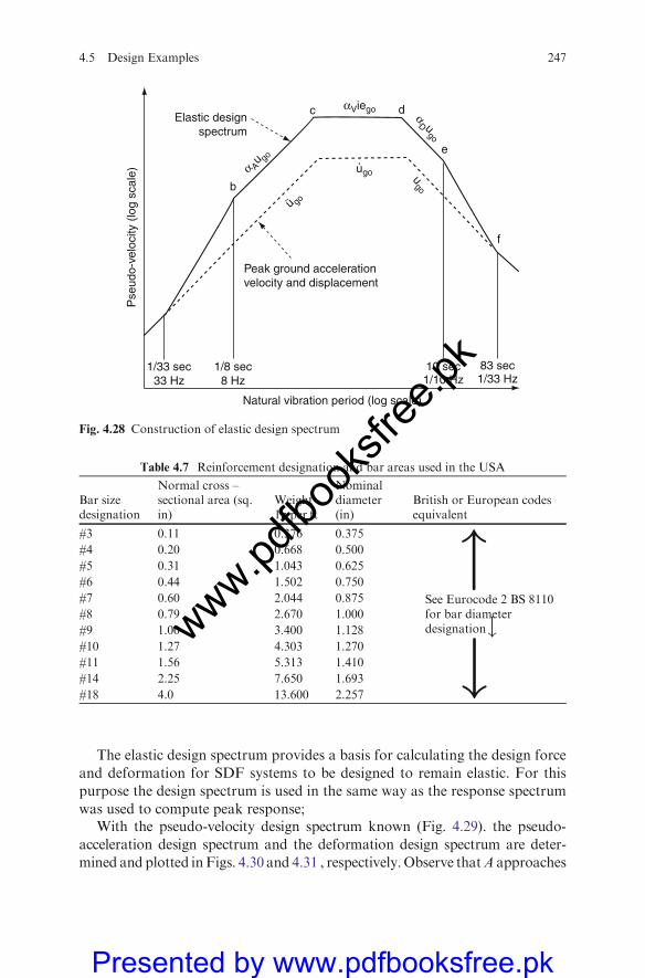
The elastic design spectrum provides a basis for calculating the design force
and deformation for SDF systems to be designed to remain elastic. For this
purpose the design spectrum is used in the same way as the response spectrum
was used to compute peak response;With the pseudo-velocity design spectrum known (Fig. 4.29). the pseudo-
acceleration design spectrum and the deformation design spectrum are deter-
mined and plotted inFigs. 4.30 and 4.31 , respectively. Observe thatA approaches
Natural vibration period (log scale)
Pse
udo-
velo
city
(lo
g sc
ale)
Elastic designspectrum
Peak ground accelerationvelocity and displacement
1/8 sec8 Hz
10 sec1/10 Hz
83 sec1/33 Hz
1/33 sec33 Hz
αViego
α Au go
αD u
go
d
e
c
b
fu
go
ü go
ugo
Fig. 4.28 Construction of elastic design spectrum
Table 4.7 Reinforcement designation and bar areas used in the USA
Bar sizedesignation
Normal cross –sectional area (sq.in)
Weight1b per ft
Nominaldiameter(in)
British or European codesequivalent
#3 0.11 0.376 0.375
See Eurocode 2 BS 8110for bar diameterdesignation#
#4 0.20 0.668 0.500
#5 0.31 1.043 0.625
#6 0.44 1.502 0.750
#7 0.60 2.044 0.875
#8 0.79 2.670 1.000
#9 1.00 3.400 1.128
#10 1.27 4.303 1.270
#11 1.56 5.313 1.410
#14 2.25 7.650 1.693
#18 4.0 13.600 2.257
"#
4.5 Design Examples 247
www.pdfbo
oksfr
ee.pk
Presented by www.pdfbooksfree.pk
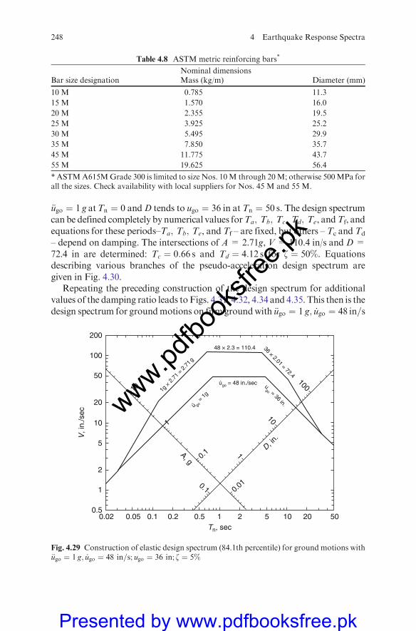
€ugo ¼ 1 g atTn ¼ 0 andD tends to ugo ¼ 36 in at Tn ¼ 50 s. The design spectrumcan be defined completely by numerical values forTa; Tb; Tc; Td; Te, andTf, andequations for these periods–Ta; Tb; Te, and Tf – are fixed, but others – Tc and Td
– depend on damping. The intersections of A= 2.71g, V= 110.4 in/s and D=72.4 in are determined: Tc ¼ 0:66 s and Td ¼ 4:12 s for z ¼ 50%. Equationsdescribing various branches of the pseudo-acceleration design spectrum aregiven in Fig. 4.30.
Repeating the preceding construction of the design spectrum for additionalvalues of the damping ratio leads toFigs. 4.31, 4.32, 4.34 and 4.35. This then is thedesign spectrum for groundmotions on firm groundwith €ugo ¼ 1 g; _ugo ¼ 48 in=s
200
10
A, g
0.1 0.01
D, in.
1g ×
2.7
1 =
2.71
g
100
50
20
10
5
2
1
0.50.02 0.05 0.1 0.2 0.5 1 2 5 10 20 50
Tn, sec
V, i
n./s
ec
48 × 2.3 = 110.4
ugo = 48 in./sec
ü go =
1g
36 × 2.01 = 72.4
ugo = 36 in.
100
1
0.1 1
10
Fig. 4.29 Construction of elastic design spectrum (84.1th percentile) for ground motions with€ugo ¼ 1 g; _ugo ¼ 48 in=s; ugo ¼ 36 in; z ¼ 5%
Table 4.8 ASTM metric reinforcing bars*
Bar size designationNominal dimensionsMass (kg/m) Diameter (mm)
10 M 0.785 11.3
15 M 1.570 16.0
20 M 2.355 19.5
25 M 3.925 25.2
30 M 5.495 29.9
35 M 7.850 35.7
45 M 11.775 43.7
55 M 19.625 56.4
* ASTMA615MGrade 300 is limited to size Nos. 10M through 20M; otherwise 500MPa forall the sizes. Check availability with local suppliers for Nos. 45 M and 55 M.
248 4 Earthquake Response Spectra
www.pdfbo
oksfr
ee.pk
Presented by www.pdfbooksfree.pk
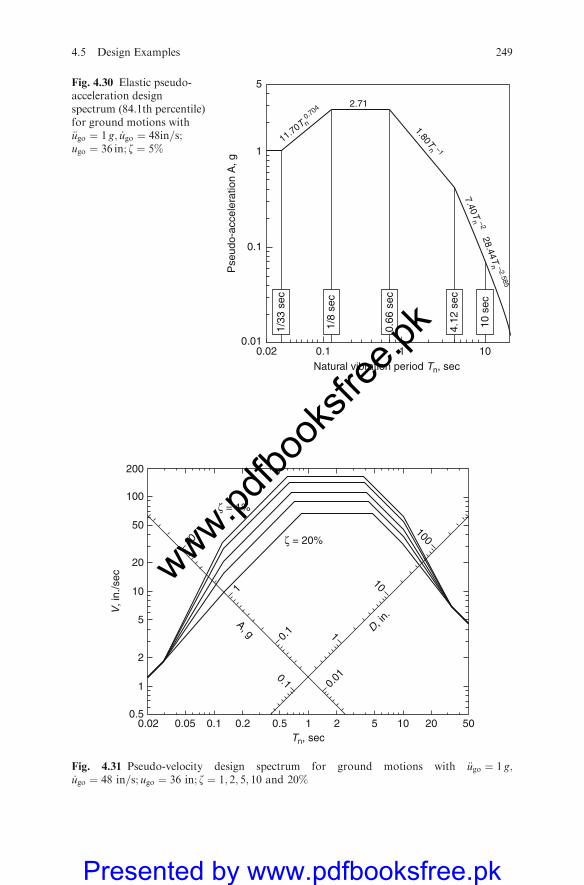
200
100
50
20
10
5
2
1
0.50.02 0.05 0.1 0.2 0.5
Tn, sec
V, i
n./s
ec
ζ = 20%
ζ = 1%
1 2 5 10 20 50
A, g
0.1 0.01
D, in.
0.1
1
10
1
10
100
Fig. 4.31 Pseudo-velocity design spectrum for ground motions with €ugo ¼ 1 g;_ugo ¼ 48 in=s; ugo ¼ 36 in; z ¼ 1; 2; 5; 10 and 20%
5
2.71
1.80Tn –1
7.40Tn –2
28.44Tn –2.585
11.70T n0.704
1
0.1
1/33
sec
1/8
sec
0.66
sec
4.12
sec
10 s
ec
0.010.02 0.1
Natural vibration period Tn, sec
Pse
udo-
acce
lera
tion
A, g
1 10
Fig. 4.30 Elastic pseudo-acceleration designspectrum (84.1th percentile)for ground motions with€ugo ¼ 1 g; _ugo ¼ 48in=s;ugo ¼ 36 in; z ¼ 5%
4.5 Design Examples 249
www.pdfbo
oksfr
ee.pk
Presented by www.pdfbooksfree.pk

200
100
50
20
10
5
2
1
0.5
1/33
sec
0.66
sec
4.12
sec
10 s
ec
33 s
ec
1/8
sec
D, i
n.
0.2
0.1
0.05
0.02
0.01
0.0050.02 0.05 0.1 0.2 0.5 1 2 5 10 30 50
Tn, sec
Fig. 4.33 Deformation design spectrum (84.1th percentile) for ground motions with€ugo ¼ 1 g; _ugo ¼ 48 in=s; ugo ¼ 36 in; z ¼ 5%
ζ = 1%
ζ = 20%
Tn, sec0.02
0.01
0.1
A, g
1
5
0.1 1 10 20
Fig. 4.32 Pseudo-acceleration designspectrum (84.1th percentile)for ground motions with€ugo ¼ 1 g; _ugo ¼ 48 in=s;ugo ¼ 36 in; z ¼ 1; 2; 5; 10and 20%
250 4 Earthquake Response Spectra
www.pdfbo
oksfr
ee.pk
Presented by www.pdfbooksfree.pk
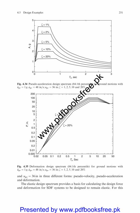
and ugo ¼ 36 in in three different forms: pseudo-velocity, pseudo-acceleration
and deformation.The elastic design spectrum provides a basis for calculating the design force
and deformation for SDF systems to be designed to remain elastic. For this
0.050.020.0050.01
0.2
0.05
0.1
0.2
1
2
510
20
50
100
200
0.1 0.2 0.5 1Tn. Sec
P, i
n.
2 5 10 20 50
0.5
ζ = 1%
ζ = 20%
Fig. 4.35 Deformation design spectrum (84.1th percentile) for ground motions with€ugo ¼ 1 g; _ugo ¼ 48 in=s; ugo ¼ 36 in; z ¼ 1; 2; 5; 10 and 20%
5
4
3
2
1
010
Tn, sec
A, g
32
ζ = 1%
ζ = 2%
ζ = 5%
ζ = 10%
ζ = 20%
Fig. 4.34 Pseudo-acceleration design spectrum (84.1th percentile) for ground motions with€ugo ¼ 1 g; _ugo ¼ 48 in=s; ugo ¼ 36 in; z ¼ 1; 2; 5; 10 and 20%
4.5 Design Examples 251
www.pdfbo
oksfr
ee.pk
Presented by www.pdfbooksfree.pk
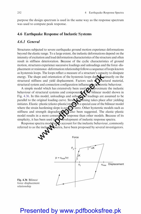
purpose the design spectrum is used in the same way as the response spectrumwas used to compute peak response.
4.6 Earthquake Response of Inelastic Systems
4.6.1 General
Structures subjected to severe earthquake ground motion experience deformationsbeyond the elastic range. To a large extent, the inelastic deformations depend on theintensityof excitationand loaddeformation characteristicsof the structure andoftenresult in stiffness deterioration. Because of the cyclic characteristics of groundmotion, structures experience successive loadings and unloadings and the force–dis-placementor resistance–deformationrelationship followsasequenceof loopsknownas hysteresis loops. The loops reflect a measure of a structure’s capacity to dissipateenergy. The shape and orientation of the hysteresis loops depend primarily on thestructural stiffness and yield displacement. Factors such as structural material,structural system and connection configuration influence the hysteretic behaviour.
A simple model which has extensively been used to approximate the inelasticbehaviour of structural systems and components is the bilinear model shown inFig. 4.36. In this model, unloadings and subsequent loadings are assumed to beparallel to the original loading curve. Strain hardening takes place after yieldinginitiates. Elastic–plastic (elasto-plastic)model is a special case of the bilinearmodelwhere the strain hardening slope is equal to zero. Other hysteretic models such asstiffness and strength degrading have also been suggested. The elastic–plasticmodel results in a more conservative response than other models. Because of itssimplicity, it has been used in the development of inelastic response spectra.
Response spectra modified to account for the inelastic behaviour, commonlyreferred to as the inelastic spectra, have been proposed by several investigators.
Displacementumaxuγ
l
l
K
αKFy
Force
μ = umax/uγ
Fig. 4.36 Bilinearforce–displacementrelationship
252 4 Earthquake Response Spectra
www.pdfbo
oksfr
ee.pk
Presented by www.pdfbooksfree.pk
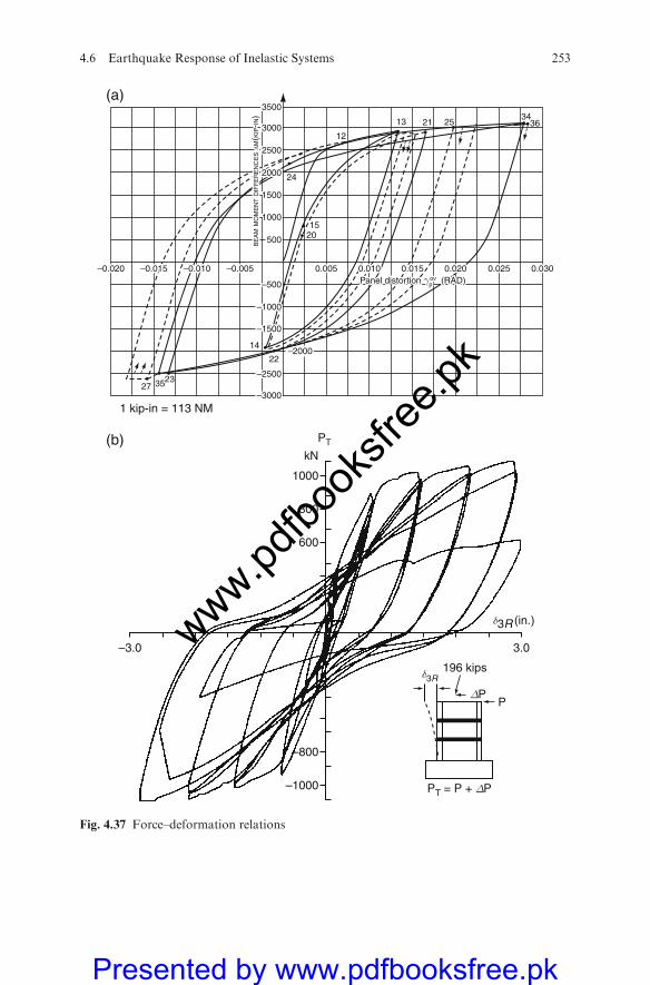
3500
2500
–2500
1500
–1500
3000
–3000
2000
–2000
1000
–1000
500
–500
–0.020 0.020 0.025 0.030–0.015 0.015–0.010 0.010–0.005 0.005
BE
AM
MO
ME
NT D
IFF
ER
EN
CE
S Δ
M(K
IP-IN
)
Panel distortion γpov (RAD)
3500
2500
–2500
1500
–1500
3000
–3000
2000
–200022
14
233527
1000
–1000
500
–500
–0.020 0.020 0.025 0.030–0.015 0.015–0.010 0.010–0.005 0.005
2015
252113
12
24
3634
BE
AM
MO
ME
NT D
IFF
ER
EN
CE
S Δ
M(K
IP-IN
)
(a)
Panel distortion γpov (RAD)
1000
800
–1000
–800
600
PT
PT = P + ΔP
kN
–3.0 3.0
196 kips
ΔP
δ3R
δ3R (in.)
P
(b)
1 kip-in = 113 NM
Fig. 4.37 Force–deformation relations
4.6 Earthquake Response of Inelastic Systems 253
www.pdfbo
oksfr
ee.pk
Presented by www.pdfbooksfree.pk
The use of the inelastic spectra in analysis and design, however, has been limitedto structures that can be modelled as a single degree of freedom. Procedures forutilizing inelastic spectra in the analysis and design of multi-degree-of-freedomsystems have also been developed to the extent that can be implemented indesign. Similar to elastic spectra, inelastic spectra can usually be plotted ontripartite paper for a given damping and ductility or yield deformation. Whenthe spectra are plotted for various ductilities, computations are repeated forseveral yield deformations using an iterative procedure such as finite elementand other techniques to achieve the target ductility.
In the inelastic yield spectrum (IYS), the yield displacement is plotted on thedisplacement axis; in the inelastic acceleration spectrum (IAS), the maximumforce per unit mass is plotted on the acceleration axis; and in the inelastic totaldisplacement (ITDS), the absolute maximum total displacement is plotted onthe displacement axis. For elastic–plastic behaviour, the inelastic yield spectrumand the inelastic acceleration spectrum are identical. Examples of inelasticspectra for a 5% damped elastic–plastic system for the S90W component ofEl-Centro, the Imperial Valley earthquake of 18 May 1940, are shown in Fig.4.26. The figure indicates that for inelastic yield and acceleration spectra, thecurves for various ductilities fall below the elastic curve (ductility of one),whereas for the inelastic total deformation spectra, they primarily fall abovethe elastic, particularly in the acceleration region. It should be noted thatincreasing the ductility ratio smoothes the spectra and minimizes the sharppeaks and valleys that are present in the plots.
A different presentation of inelastic spectra can always be conceived in aslightly different manner. The spectrum, referred to as the yield displacementspectrum (YDS), is plotted similar to the inelastic total deformation spectrumexcept that it is plotted for a given yield displacement instead of a givenductility. The ductility is obtained as the ratio of the maximum displacementto the yield displacement for which the spectrum is plotted. Their procedureoffers an efficient computational technique, particularly when statistical studiesare used to obtain inelastic design spectra.Note: This concept is fully described in the archives on Imperial Valley in theLibrary of American Congress, Washington D.C.
4.6.2 De-amplification Factors
When inelastic deformations are permitted in design, the elastic forces can bereduced if adequate ductility is provided.
Hence they presented a set of coefficients referred to as ‘‘de-amplificationfactors’’ by which the ordinates of the elastic design spectrum are multiplied toobtain the inelastic yield spectrum. In addition it is worthwhile to note that artificialaccelerograms with variable durations of strong motion presented a set of coeffi-cients referred to as ‘‘inelastic acceleration response ratios’’ by which the ordinatesof the elastic spectrum are decided to give the inelastic yield spectrum. Since these
254 4 Earthquake Response Spectra
www.pdfbo
oksfr
ee.pk
Presented by www.pdfbooksfree.pk
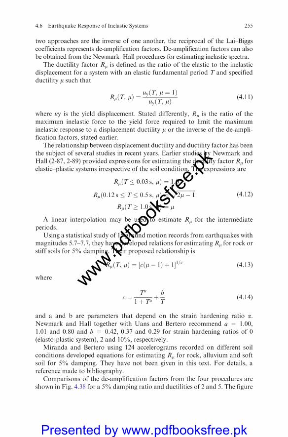
two approaches are the inverse of one another, the reciprocal of the Lai–Biggscoefficients represents de-amplification factors. De-amplification factors can alsobe obtained from the Newmark–Hall procedures for estimating inelastic spectra.
The ductility factor Rm is defined as the ratio of the elastic to the inelasticdisplacement for a system with an elastic fundamental period T and specifiedductility m such that
RmðT; mÞ ¼uyðT; m ¼ 1ÞuyðT; mÞ
(4:11)
where uy is the yield displacement. Stated differently, Rm is the ratio of themaximum inelastic force to the yield force required to limit the maximuminelastic response to a displacement ductility m or the inverse of the de-ampli-fication factors, stated earlier.
The relationship between displacement ductility and ductility factor has beenthe subject of several studies in recent years. Earlier studies by Newmark andHall (2-87, 2-89) provided expressions for estimating the ductility factor Rm forelastic–plastic systems irrespective of the soil condition. The expressions are
Rm T � 0:03 s; mð Þ ¼ 1:0
Rm 0:12 s � T � 0:5 s; mð Þ ¼ffiffiffiffiffiffiffiffiffiffiffiffiffiffi2m� 1
pRm T � 1:0 s; mð Þ ¼ m
(4:12)
A linear interpolation may be used to estimate Rm for the intermediateperiods.
Using a statistical study of 15 ground motion records from earthquakes withmagnitudes 5.7–7.7, they have developed relations for estimatingRm for rock orstiff soils for 5% damping. Their proposed relationship is
RmðT; mÞ ¼ cðm� 1Þ þ 1½ �1=c (4:13)
where
c ¼ Ta
1þ Taþ b
T(4:14)
and a and b are parameters that depend on the strain hardening ratio a.Newmark and Hall together with Uans and Bertero recommend a = 1.00,1.01 and 0.80 and b = 0.42, 0.37 and 0.29 for strain hardening ratios of 0(elasto-plastic system), 2 and 10%, respectively.
Miranda and Bertero using 124 accelerograms recorded on different soilconditions developed equations for estimating Rm for rock, alluvium and softsoil for 5% damping. They have not been given in this text. For details, areference made to bibliography.
Comparisons of the de-amplification factors from the four procedures areshown in Fig. 4.38 for a 5% damping ratio and ductilities of 2 and 5. The figure
4.6 Earthquake Response of Inelastic Systems 255
www.pdfbo
oksfr
ee.pk
Presented by www.pdfbooksfree.pk
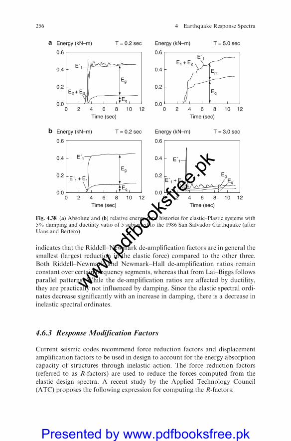
indicates that the Riddell–Newmark de-amplification factors are in general the
smallest (largest reduction in the elastic force) compared to the other three.
Both Riddell–Newmark and Newmark–Hall de-amplification ratios remain
constant over certain frequency segments, whereas that from Lai–Biggs follows
parallel patterns. While the de-amplification ratios are affected by ductility,
they are practically not influenced by damping. Since the elastic spectral ordi-
nates decrease significantly with an increase in damping, there is a decrease in
inelastic spectral ordinates.
4.6.3 Response Modification Factors
Current seismic codes recommend force reduction factors and displacement
amplification factors to be used in design to account for the energy absorption
capacity of structures through inelastic action. The force reduction factors
(referred to as R-factors) are used to reduce the forces computed from the
elastic design spectra. A recent study by the Applied Technology Council
(ATC) proposes the following expression for computing the R-factors:
20 4 6Time (sec)
8 10 12
0.6
0.4
0.2
0.0
T = 0.2 secEnergy (kN–m)
20 4 6Time (sec)
8 10 12
0.6
0.4
0.2
0.0
T = 3.0 secEnergy (kN–m)
20 4 6Time (sec)
8 10 12
0.6
0.4
0.2
0.0
T = 0.2 secEnergy (kN–m)
20 4 6Time (sec)
8 10 12
0.6
0.4
0.2
0.0
T = 5.0 secEnergy (kN–m)
E´1
E´1
E2 + E3
E1 + E2
E´1 + E1E´1 + E1
E´1E´1
Eg
EgEg
Eg
Eq
Eq
Eq
Eq
a
b
Fig. 4.38 (a) Absolute and (b) relative energy time histories for elastic–Plastic systems with5% damping and ductility vatio of 5 subjeated to the 1986 San Salvador Carthquake (afterUans and Bertero)
256 4 Earthquake Response Spectra
www.pdfbo
oksfr
ee.pk
Presented by www.pdfbooksfree.pk
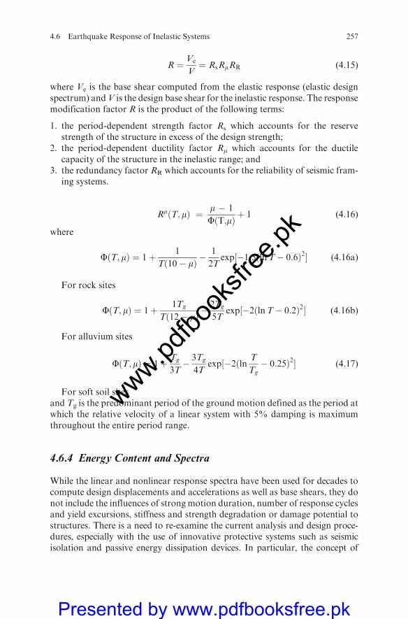
R ¼ Ve
V¼ RsRmRR (4:15)
where Ve is the base shear computed from the elastic response (elastic designspectrum) andV is the design base shear for the inelastic response. The responsemodification factor R is the product of the following terms:
1. the period-dependent strength factor Rs which accounts for the reservestrength of the structure in excess of the design strength;
2. the period-dependent ductility factor Rm which accounts for the ductilecapacity of the structure in the inelastic range; and
3. the redundancy factor RR which accounts for the reliability of seismic fram-ing systems.
RmðT; mÞ ¼ m � 1
FðT;mÞ þ 1 (4:16)
where
FðT; mÞ ¼ 1þ 1
Tð10� mÞ �1
2Texp½�1:5ðlnT� 0:6Þ2� (4:16a)
For rock sites
FðT; mÞ ¼ 1þ 1Tg
Tð12� mÞ �2Tg
5Texp½�2ðlnT� 0:2Þ2� (4:16b)
For alluvium sites
FðT; mÞ ¼ 1þ Tg
3T� 3Tg
4Texp½�2ðln T
Tg� 0:25Þ2� (4:17)
For soft soil sitesand Tg is the predominant period of the ground motion defined as the period atwhich the relative velocity of a linear system with 5% damping is maximumthroughout the entire period range.
4.6.4 Energy Content and Spectra
While the linear and nonlinear response spectra have been used for decades tocompute design displacements and accelerations as well as base shears, they donot include the influences of strong motion duration, number of response cyclesand yield excursions, stiffness and strength degradation or damage potential tostructures. There is a need to re-examine the current analysis and design proce-dures, especially with the use of innovative protective systems such as seismicisolation and passive energy dissipation devices. In particular, the concept of
4.6 Earthquake Response of Inelastic Systems 257
www.pdfbo
oksfr
ee.pk
Presented by www.pdfbooksfree.pk
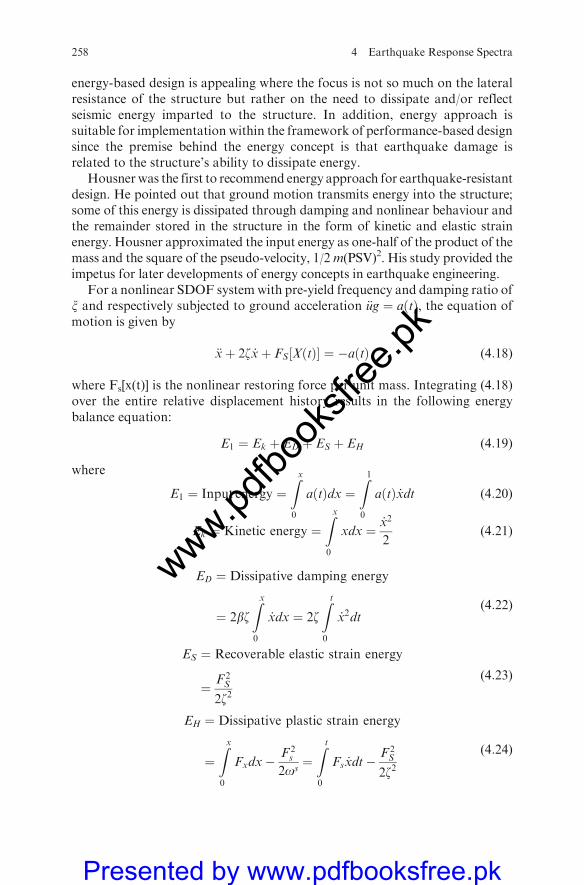
energy-based design is appealing where the focus is not so much on the lateralresistance of the structure but rather on the need to dissipate and/or reflectseismic energy imparted to the structure. In addition, energy approach issuitable for implementation within the framework of performance-based designsince the premise behind the energy concept is that earthquake damage isrelated to the structure’s ability to dissipate energy.
Housnerwas the first to recommend energy approach for earthquake-resistantdesign. He pointed out that ground motion transmits energy into the structure;some of this energy is dissipated through damping and nonlinear behaviour andthe remainder stored in the structure in the form of kinetic and elastic strainenergy. Housner approximated the input energy as one-half of the product of themass and the square of the pseudo-velocity, 1/2m(PSV)2. His study provided theimpetus for later developments of energy concepts in earthquake engineering.
For a nonlinear SDOF systemwith pre-yield frequency and damping ratio ofx and respectively subjected to ground acceleration €ug ¼ aðtÞ, the equation ofmotion is given by
€xþ 2z _xþ FS½XðtÞ� ¼ �aðtÞ (4:18)
where Fs[x(t)] is the nonlinear restoring force per unit mass. Integrating (4.18)over the entire relative displacement history results in the following energybalance equation:
E1 ¼ Ek þ ED þ ES þ EH (4:19)
where
E1 ¼ Input energy ¼Zx
0
aðtÞdx ¼Z1
0
aðtÞ _xdt (4:20)
Ek ¼ Kinetic energy ¼Zx
0
xdx ¼ _x2
2(4:21)
ED ¼ Dissipative damping energy
¼ 2bzZx
0
_xdx ¼ 2zZ t
0
_x2dt(4:22)
ES ¼ Recoverable elastic strain energy
¼ F 2S
2z2(4:23)
EH ¼ Dissipative plastic strain energy
¼Zx
0
Fxdx�F 2s
2os¼Z t
0
Fs _xdt� F 2S
2z2(4:24)
258 4 Earthquake Response Spectra
www.pdfbo
oksfr
ee.pk
Presented by www.pdfbooksfree.pk
The energy terms in the above equations are given in energy per unit mass.Through the remainder of this section, the term ‘‘energy’’ refers to the energy perunit mass. The absolute energy terms ED, ES, and EH are the same as theirrelative counterparts while the absolute input energy is given as
R€Xt dxg and the
absolute kinetic energy is given as _x2t =2where xt and xg are the absolute andground displacement, respectively. The absolute input energy represents thework done by the total base shear on the foundation displacement. The differ-ence between the absolute and relative input and kinetic energies is given by
EI:acs � EI:rel ¼
Ek:abs � Ek:rel ¼_x2g2þ _x _xg (4:25)
Figure 4.38 shows energy time histories for a short-and a long-period elastic–-plastic structure using the relative and absolute energy terms. In addition, Uangand Bertero converted the input energy to an equivalent velocity such that
VI ¼ffiffiffiffiffiffiffiffi2EI
p(4:26)
where EI can be the relative or absolute input energy per unit mass. Figure 4.38presents the relative and absolute input energy equivalent velocity spectra alongwith thepeakgroundvelocity for threeearthquakerecords.As theplots indicate, therelative and absolute input energies are very close for the mid-range periods (in thevicinity of predominant periods of groundmotion). For longer and shorter periods,however, the difference between relative and absolute energies is significant.
4.6.5 Example 4.7 American Practice
For the collapse level, the earthquake spectral design requirements are thefollowing:
Sa ¼ 0:60 gSv ¼ 21:5 in=sSd ¼ 11:9 in
Take 1 in=25.4 mmThe elastic response spectrum for a 5% damped system ductility =2%.Correct the inelastic yield spectrum:
Velocity region ¼ 1
m¼ 1
2¼ 0:5
acceleration region ¼ 1ffiffiffi2p
m� 1¼ 1ffiffiffiffiffiffiffiffiffiffiffi
4� 1p ¼ 0:58
displacement region ¼ 1
m¼ 1
2¼ 0:5
4.6 Earthquake Response of Inelastic Systems 259
www.pdfbo
oksfr
ee.pk
Presented by www.pdfbooksfree.pk
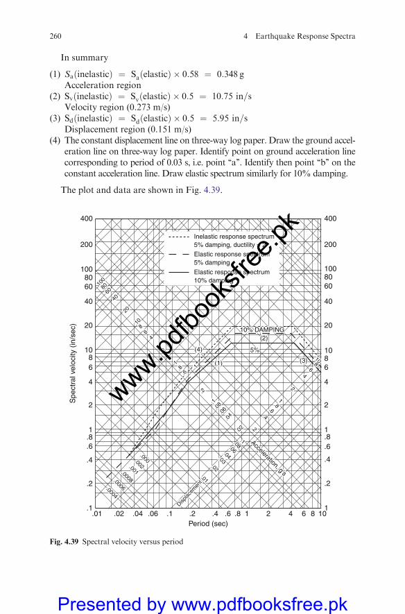
In summary
(1) SaðinelasticÞ ¼ SaðelasticÞ � 0:58 ¼ 0:348 gAcceleration region
(2) SvðinelasticÞ ¼ SvðelasticÞ � 0:5 ¼ 10:75 in=sVelocity region (0.273 m/s)
(3) SdðinelasticÞ ¼ SdðelasticÞ � 0:5 ¼ 5:95 in=sDisplacement region (0.151 m/s)
(4) The constant displacement line on three-way log paper. Draw the ground accel-eration line on three-way log paper. Identify point on ground acceleration linecorresponding to period of 0.03 s, i.e. point ‘‘a’’. Identify then point ‘‘b’’ on theconstant acceleration line. Draw elastic spectrum similarly for 10% damping.
The plot and data are shown in Fig. 4.39.
.02
.04.0
6.08.1
.2
1.6
.81
2
46
810
20
4060
8010
0
Acceleration, g's.01
.000.002.001.0008.0006.0004
.02
.03
.04
.06
.08.1
.2
.4.6
.81
2
46
810
Displac
emen
t
(3)
(2)
(1)
(4) 5%
10% DAMPING
.01 .02 .04 .06 .1 .2 .4Period (sec)
.6 .8 1 2 4 6 8 10
400
200
1008060
40
20
1086
4
2
1.8.6
.4
.2
1
400
200
1008060
40
20
Spe
ctra
l vel
ocity
(in
/sec
)
1086
4
2
1.8.6
.4
.2
.1
Inelastic response spectrum5% damping, ductility = 2
Elastic response spectrum5% damping
Elastic response spectrum10% damping
.02
.04.0
6.08.1
.2
1.6
.81
2
46
810
20
4060
8010
0
Acceleration, g's.01
.000.002.001.0008.0006.0004
.02
.03
.04
.06
.08.1
.2
.4.6
.81
2
46
810
Displac
emen
t
(3)
(2)
(1)
(4) 5%
10% DAMPING
Fig. 4.39 Spectral velocity versus period
260 4 Earthquake Response Spectra
www.pdfbo
oksfr
ee.pk
Presented by www.pdfbooksfree.pk
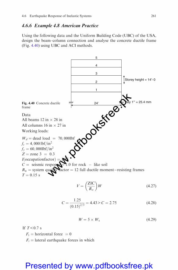
4.6.6 Example 4.8 American Practice
Using the following data and the Uniform Building Code (UBC) of the USA,
design the beam–column connection and analyse the concrete ductile frame
(Fig. 4.40) using UBC and ACI methods.
DataAll beams 12 in � 28 in
All columns 16 in � 27 in
Working loads:
Wd ¼ dead load ¼ 70; 000lbf
fc ¼ 4; 000 lbf=in2
fy ¼ 60; 000lbf=in2
Z ¼ zone 3 ¼ 0:3
IðoccupationfactorÞ ¼ 1:25
C ¼ seismic response ¼ 1:0 for rock � like soil
Rw ¼ system quality factor ¼ 12 full ductile moment�resisting frames
T ¼ 0:15 s
V ¼ ZIC
Rw
� �W (4:27)
C ¼ 1:25
ð0:15Þ2=3¼ 4:434C ¼ 2:75 (4:28)
W ¼ 5�Ws (4:29)
If T50:7 s
Ft ¼ horizontal force ¼ 0
Fi ¼ lateral earthquake forces in which
1
2
3
4
5
24' Key 1′′ = 25.4 mm
Storey height = 14′- 0
Fig. 4.40 Concrete ductileframe
4.6 Earthquake Response of Inelastic Systems 261
www.pdfbo
oksfr
ee.pk
Presented by www.pdfbooksfree.pk
Ft ¼ 0 at the ith level
¼ WihiPni¼1Wihi
� �V
(4:30)
Fi ¼ CiV ¼ 0:86CiWs (4:31)
Initial value to start with is
Xni¼1¼ ð1þ 2þ 3þ 4þ 5ÞWs ði ¼ 5 at the topmost floorÞ
All floors need to be analysed for lateral forces, storey shears and storeymoments.
Brief design notes and design formulae UBC and ACI
Relevant terms are
WS ¼ weight of one storey
RW ¼ system quality factor
W ¼ total vertical weight of building ¼ nWS
S ¼ site factor
C ¼ seismic response ¼ 1:25=Tð Þ3
n ¼ number of storeys
Step I
Determine earthquake zone, select UBC seismic coefficients Z,I,C,S,RW.Determine period T by UBC method A or B.
Step II
Compute
V ¼ ZIC
RWW and V ¼ Ft þ
Xn
i¼1 Ft (4:32)
Ft ¼ 0 when T ¼ 0:7 s
Ft ¼ 0:97TC � 0:25V
Tn ¼ CtðhwÞ3=4
Ct ¼ 0:10ffiffiffiffiffiffiffiACp
Step III
Tabulate base lateral force and each storey force Fi toFn :
262 4 Earthquake Response Spectra
www.pdfbo
oksfr
ee.pk
Presented by www.pdfbooksfree.pk
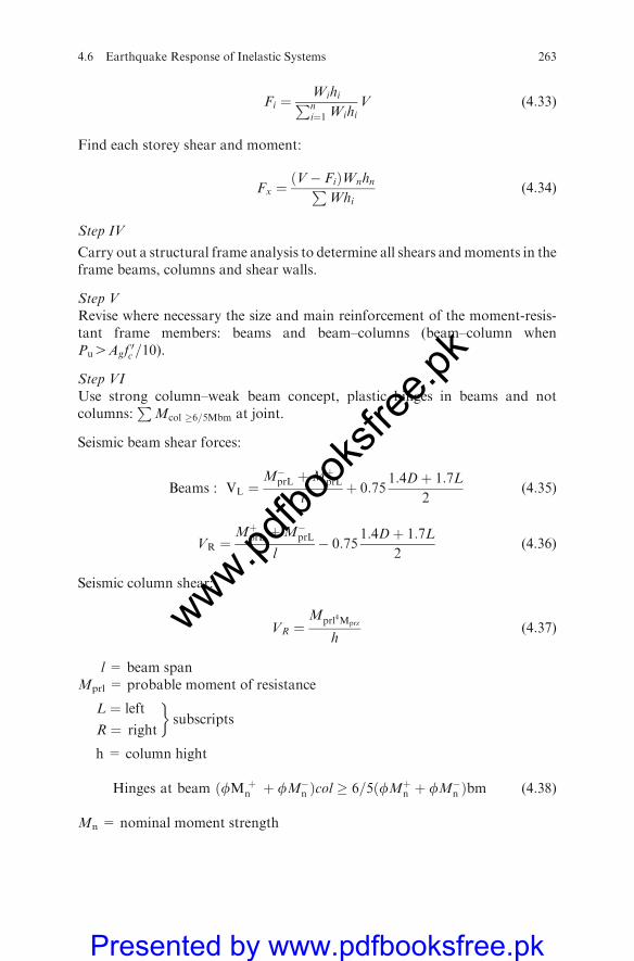
Fi ¼WihiPni¼1 Wihi
V (4:33)
Find each storey shear and moment:
Fx ¼V� Fið ÞWnhnP
Whi(4:34)
Step IV
Carry out a structural frame analysis to determine all shears andmoments in theframe beams, columns and shear walls.
Step VRevise where necessary the size and main reinforcement of the moment-resis-tant frame members: beams and beam–columns (beam–column whenPu4Agf
0c =10).
Step VIUse strong column–weak beam concept, plastic hinges in beams and notcolumns:
PMcol �6=5Mbm at joint.
Seismic beam shear forces:
Beams : VL ¼M�prL þMþprL
tþ 0:75
1:4Dþ 1:7L
2(4:35)
VR ¼MþprL þM�prL
l� 0:75
1:4Dþ 1:7L
2(4:36)
Seismic column shear:
VR ¼Mprl4Mprz
h(4:37)
l = beam spanMprl = probable moment of resistance
L ¼ left
R ¼ right
subscripts
h = column hight
Hinges at beam ðfM þn þ fM�n Þcol � 6=5ðfMþn þ fM�n Þbm (4:38)
Mn = nominal moment strength
4.6 Earthquake Response of Inelastic Systems 263
www.pdfbo
oksfr
ee.pk
Presented by www.pdfbooksfree.pk
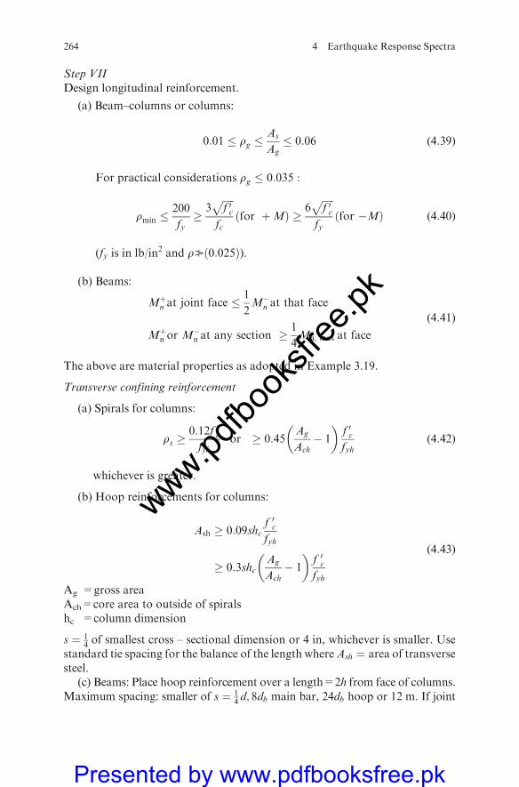
Step VIIDesign longitudinal reinforcement.
(a) Beam–columns or columns:
0:01 � rg �As
Ag� 0:06 (4:39)
For practical considerations rg � 0:035 :
rmin �200
fy�
3ffiffiffiffiffif 0c
pfc
for þMð Þ �6ffiffiffiffiffif 0c
pfy
for �Mð Þ (4:40)
(fy is in lb/in2 and rB 0:025ð Þ).
(b) Beams:
Mþn at joint face �1
2M�n at that face
Mþn or M�n at any section � 1
4Ma; max at face
(4:41)
The above are material properties as adopted in Example 3.19.
Transverse confining reinforcement
(a) Spirals for columns:
rs �0:12f 0cfyh
or � 0:45Ag
Ach� 1
� �f 0cfyh
(4:42)
whichever is greater.
(b) Hoop reinforcements for columns:
Ash � 0:09shcf 0cfyh
� 0:3shcAg
Ach� 1
� �f 0cfyh
(4:43)
Ag =gross areaAch=core area to outside of spiralshc =column dimension
s ¼ 14of smallest cross – sectional dimension or 4 in, whichever is smaller. Use
standard tie spacing for the balance of the length whereAsh ¼ area of transversesteel.
(c) Beams: Place hoop reinforcement over a length=2h from face of columns.Maximum spacing: smaller of s ¼ 1
4 d; 8db main bar, 24db hoop or 12 m. If joint
264 4 Earthquake Response Spectra
www.pdfbo
oksfr
ee.pk
Presented by www.pdfbooksfree.pk
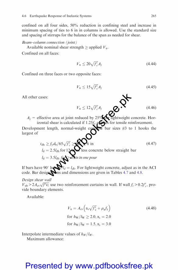
confined on all four sides, 50% reduction in confining steel and increase inminimum spacing of ties to 6 in in columns is allowed. Use the standard sizeand spacing of stirrups for the balance of the span as needed for shear.
Beam–column connection (joint)Available nominal shear strength � applied Vu.
Confined on all faces:
Vn � 20ffiffiffiffiffif 0c
pAj (4:44)
Confined on three faces or two opposite faces:
Vn � 15ffiffiffiffiffif 0c
pAj (4:45)
All other cases:
Vn � 12ffiffiffiffiffif 0c
pAj (4:46)
Aj = effective area at joint reduced by 25% for lightweight concrete. Hor-izontal shear is calculated if 1.25fy applies for tensile reinforcement.
Development length, normal-weight concrete bar sizes #3 to 1 hooks thelargest of
tdh � fydb=65ffiffiffiffiffif 0c
p� 8db � 6 in (4:47)
ld ¼ 2:5ldh for 12 in or less concrete below straight bar
ld ¼ 3:5ldh for � 12in in one pour
If bars have 908 hooks, ld ¼ ldh. For lightweight concrete, adjust as in the ACIcode. Bar designations and dimensions are given in Tables 4.7 and 4.8.
Design shear wallVuh42Acv
ffiffiffiffiffiffiffif 0c;p
use two reinforcement curtains in wall. If wall fc40:2f 0c; pro-vide boundary elements.
Available:
Vn ¼ Acv asffiffiffiffiffif 0c
pþ rnfy
� �(4:48)
for hW=lW � 2:0; as ¼ 2:0
for hW=lW ¼ 1:5; as ¼ 3:0
Interpolate intermediate values of hW=lW.Maximum allowance:
4.6 Earthquake Response of Inelastic Systems 265
www.pdfbo
oksfr
ee.pk
Presented by www.pdfbooksfree.pk
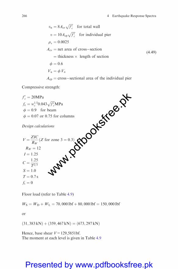
un ¼ 8Acv
ffiffiffiffiffif 0c
pfor total wall
u ¼ 10Acp
ffiffiffiffiffif 0c
pfor individual pier
rv ¼ 0:0025
Acv ¼ net area of cross�section
¼ thickness� length of section
f ¼ 0:6
Vu ¼ fVn
Acp ¼ cross�sectional area of the individual pier
(4:49)
Compressive strength:
f 0c ¼ 20MPa
fc ¼ w1:5c 0:043
ffiffiffiffiffif 0c
pMPa
f ¼ 0:9 for beam
f ¼ 0:07 or 0:75 for columns
Design calculations
V ¼ ZIC
RWðZ for zone 3 ¼ 0:3Þ
RW ¼ 12
I ¼ 1:25
C ¼ 1:25
T2=3
S ¼ 1:0
T ¼ 0:7 s
ft ¼ 0
Floor load (refer to Table 4.9)
WS ¼WD þWL ¼ 70; 000 lbfþ 80; 000 lbf ¼ 150; 000 lbf
or
31; 383 kNð Þ þ 359; 467 kNð Þ ¼ 673; 297 kNð Þ
Hence, base shear V=129,5851bf.The moment at each level is given in Table 4.9
266 4 Earthquake Response Spectra
www.pdfbo
oksfr
ee.pk
Presented by www.pdfbooksfree.pk
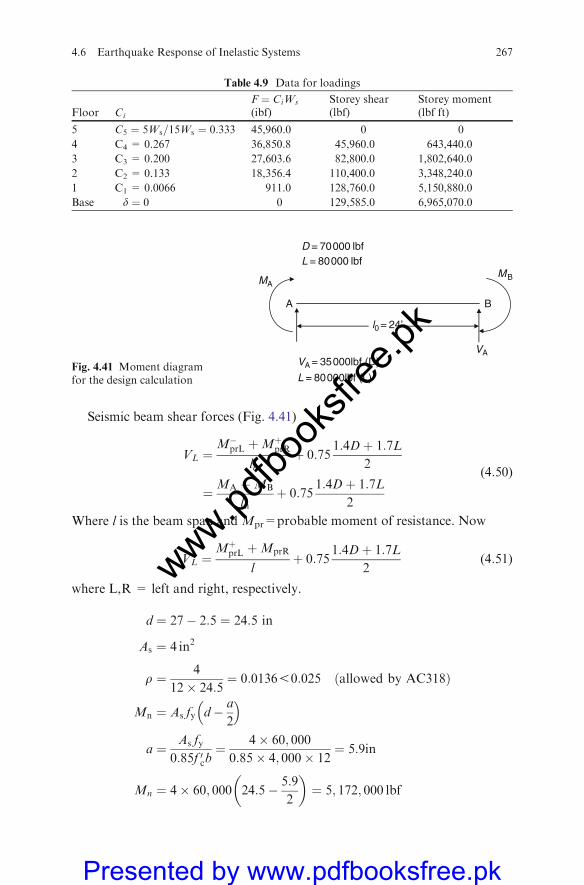
Seismic beam shear forces (Fig. 4.41)
VL ¼M�prL þMþprR
lnþ 0:75
1:4Dþ 1:7L
2
¼MA þMB
lnþ 0:75
1:4Dþ 1:7L
2
(4:50)
Where l is the beam span and Mpr=probable moment of resistance. Now
VL ¼MþprL þMprR
lþ 0:75
1:4Dþ 1:7L
2(4:51)
where L,R = left and right, respectively.
d ¼ 27� 2:5 ¼ 24:5 in
As ¼ 4 in2
r ¼ 4
12� 24:5¼ 0:013650:025 allowed by AC318ð Þ
Mn ¼ As fy d� a
2
� �
a ¼ As fy0:85f 0cb
¼ 4� 60; 000
0:85� 4; 000� 12¼ 5:9in
Mn ¼ 4� 60; 000 24:5� 5:9
2
� �¼ 5; 172; 000 lbf
Table 4.9 Data for loadings
Floor Ci
F ¼ CiWs
(ibf)Storey shear(lbf)
Storey moment(lbf ft)
5 C5 ¼ 5Ws=15Ws ¼ 0:333 45,960.0 0 0
4 C4 = 0.267 36,850.8 45,960.0 643,440.0
3 C3 = 0.200 27,603.6 82,800.0 1,802,640.0
2 C2 = 0.133 18,356.4 110,400.0 3,348,240.0
1 C1 = 0.0066 911.0 128,760.0 5,150,880.0
Base d ¼ 0 0 129,585.0 6,965,070.0
D = 70000 lbfL = 80000 lbf
MAMB
BA
VAVA = 35000lbf (D)
L = 80000lbf (L)
l0 = 24’
Fig. 4.41 Moment diagramfor the design calculation
4.6 Earthquake Response of Inelastic Systems 267
www.pdfbo
oksfr
ee.pk
Presented by www.pdfbooksfree.pk
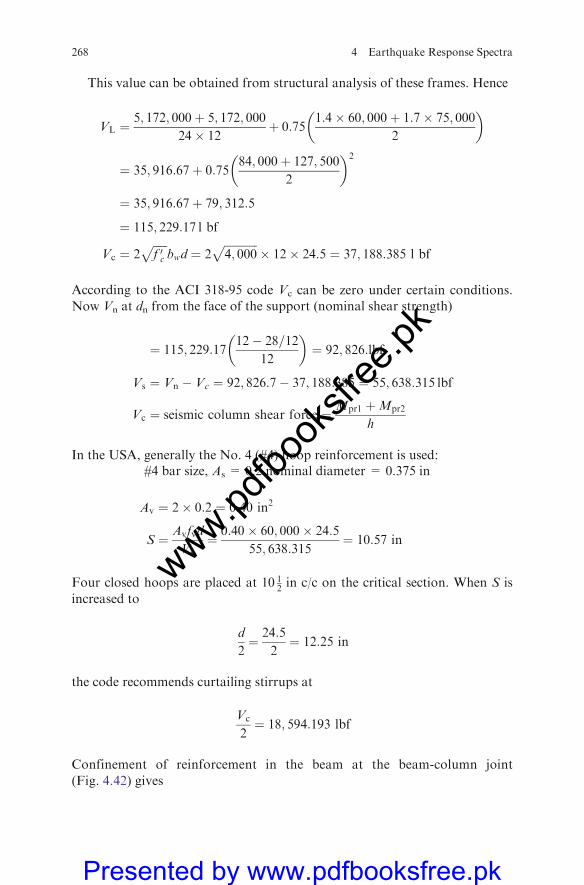
This value can be obtained from structural analysis of these frames. Hence
VL ¼5; 172; 000þ 5; 172; 000
24� 12þ 0:75
1:4� 60; 000þ 1:7� 75; 000
2
� �
¼ 35; 916:67þ 0:7584; 000þ 127; 500
2
� �2
¼ 35; 916:67þ 79; 312:5
¼ 115; 229:17 l bf
Vc ¼ 2ffiffiffiffiffif 0c
pbwd ¼ 2
ffiffiffiffiffiffiffiffiffiffiffiffi4; 000
p� 12� 24:5 ¼ 37; 188:385 l bf
According to the ACI 318-95 code Vc can be zero under certain conditions.
Now Vn at dn from the face of the support (nominal shear strength)
¼ 115; 229:1712� 28=12
12
� �¼ 92; 826:lbf
Vs ¼ Vn � Vc ¼ 92; 826:7� 37; 188:385 ¼ 55; 638:315 lbf
Vc ¼ seismic column shear force ¼Mpr1 þMpr2
h
In the USA, generally the No. 4 (#4) hoop reinforcement is used:#4 bar size, As = 0.2 nominal diameter = 0.375 in
Av ¼ 2� 0:2 ¼ 0:40 in2
S ¼ Avfvd
Vs¼ 0:40� 60; 000� 24:5
55; 638:315¼ 10:57 in
Four closed hoops are placed at 10 12in c/c on the critical section. When S is
increased to
d
2¼ 24:5
2¼ 12:25 in
the code recommends curtailing stirrups at
Vc
2¼ 18; 594:193 lbf
Confinement of reinforcement in the beam at the beam-column joint
(Fig. 4.42) gives
268 4 Earthquake Response Spectra
www.pdfbo
oksfr
ee.pk
Presented by www.pdfbooksfree.pk
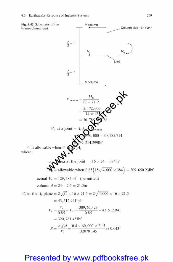
Vcolumn ¼Mn
7þ 7ð Þ12
¼ 5; 172; 000
14� 12
¼ 30; 785:714 lbf
Vn at a joint ¼ As fy � Vcolumn
¼ 4:0� 60; 000� 30; 785:714
¼ 209; 214:299lbfVn is allowable when � 15
ffiffiffiffiffif 0c
pAj
where
Aj ¼ area at the joint ¼ 16� 24 ¼ 384in2
Vu ¼ allowable when 0:85 15ffiffiffiffiffiffiffiffiffiffiffiffi4; 000
p� 384
� �¼ 309; 650:23lbf
actual Vc ¼ 129; 585lbf permittedð Þ
column d ¼ 24� 2:5 ¼ 21:5in
Vc at the Aj plane ¼ 2ffiffiffiffiffif 0c
p� 16� 21:5 ¼ 2
ffiffiffiffiffiffiffiffiffiffiffiffi4; 000
p� 16� 21:5
¼ 43; 512:941lbf
Vc ¼Vu
0:85� Vc ¼
309; 650:23
0:85� 43; 512:941
¼ 320; 781:45 lbf
S ¼ Avfvd
Vs¼ 0:4� 60; 000� 21:5
320781:45� 0:643
V column
Vu
h2
= T
V column
joint
Mu
Column size 16° x 24°
h2
= T
Fig. 4.42 Schematic of thebeam-column joint
4.6 Earthquake Response of Inelastic Systems 269
www.pdfbo
oksfr
ee.pk
Presented by www.pdfbooksfree.pk

Maximum allowable (Thus, nine # 4 bars)
S ¼ d=4 ¼ 21:5
4¼ 5:375
Adopt 3 in {i.e. 4 in diameter}
8db ¼ 8� 9
8¼ 9 in
db � 24 ¼ 24� 1
2¼ 12 in ðminimumÞ
Thus, use four hoops plus two #4 cross-ties at 3 in c/c. The length of suchhoops:
l0 ¼ 2 h ¼ 2� 28 ¼ 56 in
Reinforcement in the column at the beam-column jointWhichever Ash is greater should be adopted:
Ash � 0:009Shcf0c=fyh
or
Ash � 0:3ShcAg
Ach� 1
� �f 0cFyh
hc ¼ column core
¼ 24� ð2� 1:5þ 2� 0:5Þ ¼ 20 in
Try S = 3 in
Ash ¼ 0:09� 3� 204000
60; 000
� �¼ 0:36 in2
or
Ash ¼ 0:3� 3� 2016� 24
11� 20� 1
� �4000
60; 0000:89 in2
Now, S (maximum allowable) ¼ 14b ¼ 1
4small dimension or 4 in
¼ 14� 16 ¼ 4in
Therefore, use #4 hoops at 3 in c/c and place the confining hoops in the columnon both sides of the joint over a distance l0 using the largest of
(a) depth of the member = 24 in(b) 1
6� clear span ¼ 1
6� 24� 12 ¼ 48 in
(c) 18 in
Thus, l0 ¼ 48 in; #4 hoops and cross-ties at 3 in c/c spacing (Fig. 4.43).
270 4 Earthquake Response Spectra
www.pdfbo
oksfr
ee.pk
Presented by www.pdfbooksfree.pk
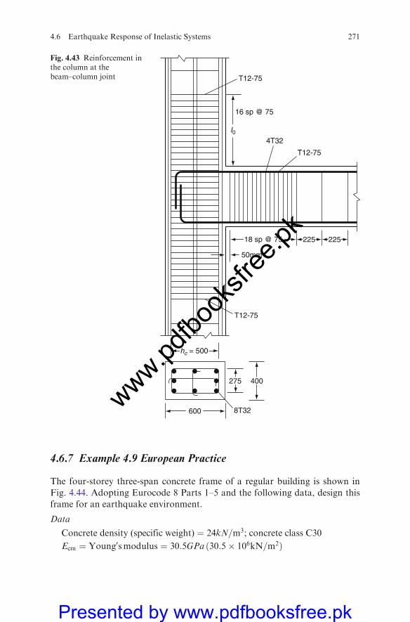
4.6.7 Example 4.9 European Practice
The four-storey three-span concrete frame of a regular building is shown in
Fig. 4.44. Adopting Eurocode 8 Parts 1–5 and the following data, design this
frame for an earthquake environment.
Data
Concrete density (specific weight) ¼ 24kN=m3; concrete class C30
Ecm ¼ Young0smodulus ¼ 30:5GPa ð30:5� 106kN=m2Þ
600 8T32
275
T12-75
50mm
T12-75
T12-75
I04T32
16 sp @ 75
22518 sp @ 75 225
400
hc = 500
Fig. 4.43 Reinforcement inthe column at thebeam–column joint
4.6 Earthquake Response of Inelastic Systems 271
www.pdfbo
oksfr
ee.pk
Presented by www.pdfbooksfree.pk

v ¼ Poisson0s ratio ¼ 0:2
fck=gc ¼ design compressive strength ¼ 30=1:5 ¼ 20MPa ð20MN=m2Þ
TRd ¼ design shear strength ¼ 0:30MPa ð0:3MN=m2Þ
hc ¼ 3:0m
h1 ¼ 4:0m
All columns 1� 2 levels ¼ 500� 500; all beams at 1� 2 levels ¼ 400� 400:
All columns 2� 3 levels ¼ 500� 500; all beams at 2� 3 levels ¼ 400� 400:
All columns 3� 4 and 4� 5 levels ¼ 400� 400:
All beams 3� 4 and 4� 5 levels ¼ 500� 500:
Eurocode classSteel class S400
fyd ¼ design tensile strength ¼ fyk=gs
¼ 400=1:15 ¼ 348MPa ð348MN=m2Þ
Design loads
g ¼ dead load ðfloor; slabs; finishes; etc:Þ ¼ 6kN=m2
G ¼ 6kN=m2 � 5:0m ¼ 30kN=m
1
2
3
4
5 6
7
8
9
10
11
12
13
14
15
16
17
18
19
20
h1
h2
h3
h4
Frame dimensions
3 @ 5.0 m
Fig. 4.44 Frame dimensionsfor Example 4.9
272 4 Earthquake Response Spectra
www.pdfbo
oksfr
ee.pk
Presented by www.pdfbooksfree.pk
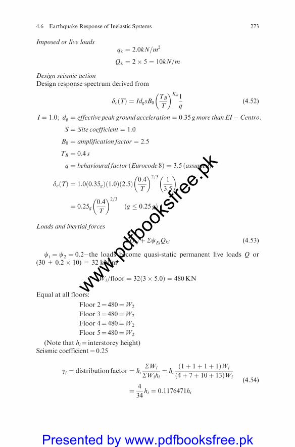
Imposed or live loadsqk ¼ 2:0kN=m2
Qk ¼ 2� 5 ¼ 10kN=m
Design seismic actionDesign response spectrum derived from
dcðTÞ ¼ IdgsB0TB
T
� �Kdt1
q(4:52)
I ¼ 1:0; dg ¼ effective peak ground acceleration ¼ 0:35 gmore thanEI� Centro:
S ¼ Site coefficient ¼ 1:0
B0 ¼ amplification factor ¼ 2:5
TB ¼ 0:4 s
q ¼ behavioural factor ðEurocode 8Þ ¼ 3:5 ðassumedÞ
deðTÞ ¼ 1:0ð0:35gÞð1:0Þð2:5Þ0:4
T
� �2=31
3:5
� �
¼ 0:25g0:4
T
� �2=3
ðg � 0:25 gÞ
Loads and inertial forces
SGkj þ ScEiQki (4:53)
ci ¼ c2 ¼ 0:2�the loads become quasi-static permanent live loads Q or(30 + 0.2 � 10) = 32 kN/m
Wi=floor ¼ 32ð3� 5:0Þ ¼ 480KN
Equal at all floors:
Floor 2¼ 480¼W2
Floor 3¼ 480¼W2
Floor 4¼ 480¼W2
Floor 5¼ 480¼W2
(Note that hi¼ interstorey height)Seismic coefficient¼ 0.25
gi ¼ distribution factor ¼ hiSWi
SWihi¼ hi
ð1þ 1þ 1þ 1ÞWi
ð4þ 7þ 10þ 13ÞWi
¼ 4
34hi ¼ 0:1176471hi
(4:54)
4.6 Earthquake Response of Inelastic Systems 273
www.pdfbo
oksfr
ee.pk
Presented by www.pdfbooksfree.pk

Horizontal forces at each levelThe method has been demonstrated in other examples and the horizontal forces
are computed (Fig. 4.45).
Load combination for structural analysisEurocode 8 specifies at least two load combinations: (a) with the live load as themain variable action and (b) with the seismic load as the main action:
ðaÞ Sd ¼ Sð1:35Gþ 1:5QkÞðbÞ Sd ¼ SðGþ SciQk þ EÞ
load combinations
The frame has been analysed for these two loading cases using an IBM PC andthe above data with the program STIFF. Design moments are based on thelinear analysis of the building frame. Redistribution is permitted (see Fig. 4.46).
(A) BeamsFrom seismically considered situations, all beams shall be equally reinforced tocover 40 mm or 4 cm beams of 500�500.
MRd ¼ the ultimate bending moment at:
positive ¼ 240kNm4145
negative ¼ 355kNm � 265
See Table 4.10 for data.Design shear forcesConditions of static equilibrium at the beams subjected to vertical loads and endmoments give design shear forces. The end moments must be from the actualreinforcement placed in beams. Eurocode 2 suggests the following beam analysisto evaluate moments and reactions. Each section at the end shall have two values ofshear force – the maximum and the minimum value corresponding to positive andnegative moments yielding at the hinges. The algebraic ratio between the maximumand the minimum values of the shear force at a section shall be denoted by ‘‘z’’. Forthepurposes of design the value of z shall not be takenas smaller than�1 (Fig. 4.47).
Floor 4
Floor 3
Floor 2
Floor 1
183.7 KN
141.4
98.85
56.55
Fig. 4.45 Horizontal forcesat each level of frame
274 4 Earthquake Response Spectra
www.pdfbo
oksfr
ee.pk
Presented by www.pdfbooksfree.pk
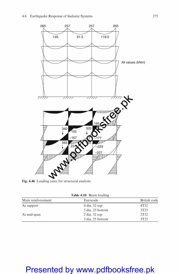
265 257 257 265
91.5 118.0145
All values (kNm)
–227–250
–167
155
231 –229
–177
165
320
535565
340
Fig. 4.46 Loading cases for structural analysis
Table 4.10 Beam loading
Main reinforcement Eurocode British code
At support 4 dia. 32 top 4T32
3 dia. 25 bottom 3T25
At mid-span 2 dia. 32 top 2T32
3 dia. 25 bottom 3T25
4.6 Earthquake Response of Inelastic Systems 275
www.pdfbo
oksfr
ee.pk
Presented by www.pdfbooksfree.pk
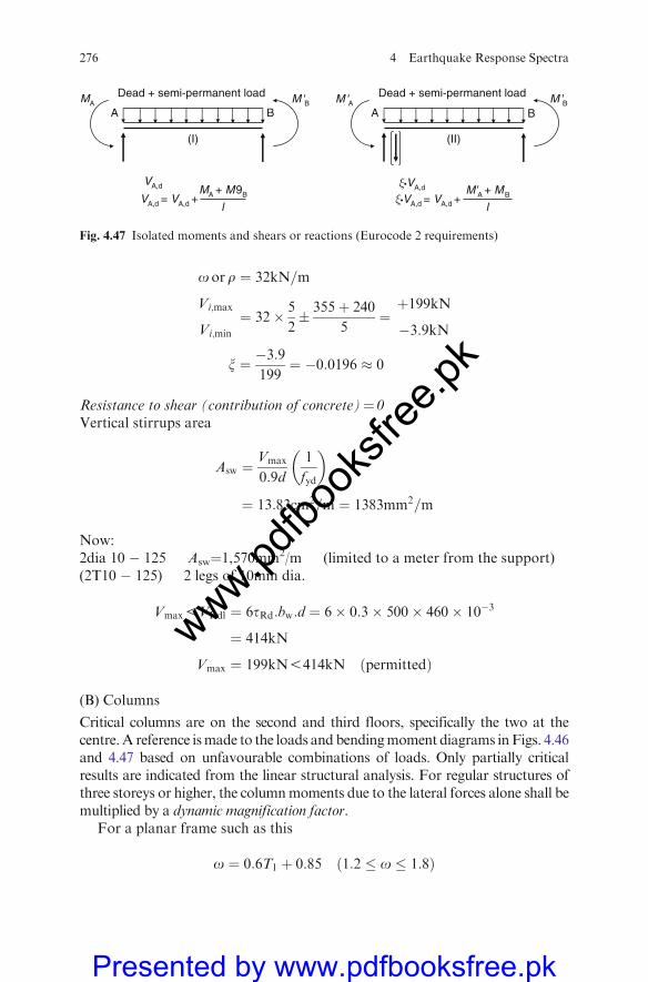
o or r ¼ 32kN=m
Vi;max
Vi;min
¼ 32� 5
2� 355þ 240
5¼þ199kN
�3:9kN
x ¼ �3:9199
¼ �0:0196 � 0
Resistance to shear (contribution of concrete)¼ 0Vertical stirrups area
Asw ¼Vmax
0:9d
1
fyd
� �
¼ 13:83cm2=m ¼ 1383mm2=m
Now:2dia 10 � 125 Asw¼1,570mm2/m (limited to a meter from the support)(2T10 � 125) 2 legs of 10mm dia.
Vmax5VRdl ¼ 6tRd:bw:d ¼ 6� 0:3� 500� 460� 10�3
¼ 414kN
Vmax ¼ 199kN5414kN ðpermittedÞ
(B) Columns
Critical columns are on the second and third floors, specifically the two at thecentre.A reference ismade to the loads and bendingmoment diagrams inFigs. 4.46and 4.47 based on unfavourable combinations of loads. Only partially criticalresults are indicated from the linear structural analysis. For regular structures ofthree storeys or higher, the columnmoments due to the lateral forces alone shall bemultiplied by a dynamic magnification factor.
For a planar frame such as this
o ¼ 0:6T1 þ 0:85 1:2 � o � 1:8ð Þ
Dead + semi-permanent load MA M'BBA
(I)
Dead + semi-permanent load M'A M'BBA
(II)
VA,d
VA,d = VA,d +MA + M9B
l
ξ•VA,d
ξ•VA,d = VA,d +M'A + MB
l
Fig. 4.47 Isolated moments and shears or reactions (Eurocode 2 requirements)
276 4 Earthquake Response Spectra
www.pdfbo
oksfr
ee.pk
Presented by www.pdfbooksfree.pk
where T1 is the fundamental period of the structure T1 (Eurocode 8) is in therange of 0.4–0.6. Hence
o ¼ 0:6ð0:6Þ þ 0:85 ¼ 1:1241:3
Therefore, o ¼ 1:3 is retained.
Relative strength between columns and beams at jointThis requirement of Eurocode 8 is to be adhered to. Thus
Mb ¼ sumof beammoments ¼ MþRD þM�RD
� �¼ 240þ 355ð Þ ¼ 595kNm
Mc ¼ sum of column design moments
¼ 1:3 155 þ 231ð Þ ¼ 501:8kNm
ReinforcementAdverse combinations of axial forceN and bending momentM can be adopted:
upper column
N ¼ 320kN
M ¼ 1:3� 177 ¼ 230:1kNm
lower column
N ¼ 565kN
M ¼ 1:3� 227 ¼ 295:1kNm
The section is therefore checked. Actual reinforcement provided in the section(avoiding traditional column calculations) is
8 dia: 25 and 12dia: 20 Eurocode
8T25ð Þ 12T20ð Þ British standard
As ¼ 3; 932mm2 As ¼ 3; 760mm2
Total AsToT ¼ 7; 692mm2
The corresponding ultimate bending moments:upper column
MRdu ¼ 265kNm4230:1kNm
4.6 Earthquake Response of Inelastic Systems 277
www.pdfbo
oksfr
ee.pk
Presented by www.pdfbooksfree.pk
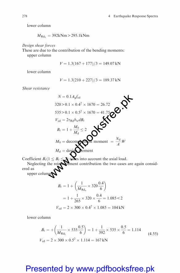
lower column
MRdL ¼ 392kNm4295:1kNm
Design shear forcesThese are due to the contribution of the bending moments:
upper column
V ¼ 1:3 167þ 177ð Þ=3 ¼ 149:07 kN
lower column
V ¼ 1:3 210þ 227ð Þ=3 ¼ 189:37 kN
Shear resistance
N ¼ 0:1Agfcd
32040:1� 0:42 � 1670 ¼ 26:72
53540:1� 0:52 � 1670 ¼ 41:75
Vcd ¼ 2tRdbwdB‘
B‘ ¼ 1þM0
Md� 2
M0 ¼ decompression moment ¼ Nd
AW
Md ¼ design moment
Coefficient B‘ 1 � B‘ � 2ð Þ takes into account the axial load.Neglecting the reinforcement contribution the two cases are again consid-
ered asupper column
B‘ ¼ 1þ 1
MRdu
� 3200:4
6
� �
¼ 1þ 1
265� 320� 0:4
6¼ 1:08552
Vcd ¼ 2� 300� 0:42 � 1:085 ¼ 104 kN
lower column
B‘ ¼ þ1
MRdL
� 5350:5
6
� �¼ 1þ 1
392� 535� 0:5
6¼ 1:114
Vcd ¼ 2� 300� 0:52 � 1:114 ¼ 167 kN
(4:55)
278 4 Earthquake Response Spectra
www.pdfbo
oksfr
ee.pk
Presented by www.pdfbooksfree.pk
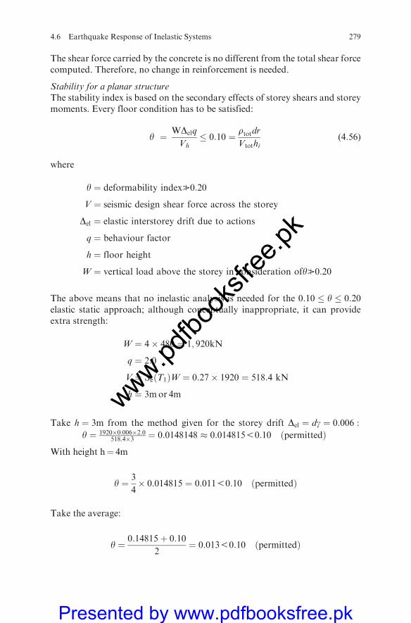
The shear force carried by the concrete is no different from the total shear forcecomputed. Therefore, no change in reinforcement is needed.
Stability for a planar structureThe stability index is based on the secondary effects of storey shears and storeymoments. Every floor condition has to be satisfied:
y ¼ WDelq
Vh� 0:10 ¼ rtotdr
Vtothi(4:56)
where
y ¼ deformability indexB0:20
V ¼ seismic design shear force across the storey
Del ¼ elastic interstorey drift due to actions
q ¼ behaviour factor
h ¼ floor height
W ¼ vertical load above the storey in consideration ofyB0:20
The above means that no inelastic analysis is needed for the 0:10 � y � 0:20elastic static approach; although conceptually inappropriate, it can provideextra strength:
W ¼ 4� 480 ¼ 1; 920kN
q ¼ 2:0
V ¼ SeðT1ÞW ¼ 0:27� 1920 ¼ 518:4 kN
h ¼ 3mor 4m
Take h ¼ 3m from the method given for the storey drift Del ¼ dg ¼ 0:006 :
y ¼ 1920�0:006�2:0518:4�3 ¼ 0:0148148 � 0:01481550:10 ðpermittedÞ
With height h¼ 4m
y ¼ 3
4� 0:014815 ¼ 0:01150:10 ðpermittedÞ
Take the average:
y ¼ 0:14815 þ 0:10
2¼ 0:01350:10 ðpermittedÞ
4.6 Earthquake Response of Inelastic Systems 279
www.pdfbo
oksfr
ee.pk
Presented by www.pdfbooksfree.pk
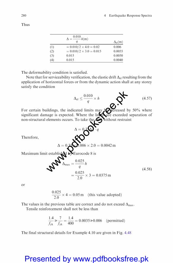
Thus
D ¼ 0:010
qhðmÞ
DelðmÞ(1) ¼ 0:010=2� 4:0 ¼ 0:02 0.006
(2) ¼ 0:010=2� 3:0 ¼ 0:015 0.0055
(3) 0.015 0.0050
(4) 0.015 0.0040
The deformability condition is satisfied.Note that for serviceability verification, the elastic driftDel resulting from the
application of horizontal forces or from the dynamic action shall at any storeysatisfy the condition
Del �0:010
q� h (4:57)
For certain buildings, the indicated limits may be increased by 50% wheresignificant damage is expected. Where the limits are exceeded separation ofnon-structural elements occurs. To take the drift without restraint
D ¼ 0:35Del q
Therefore,
D ¼ 0:35� 0:006� 2:0 ¼ 0:0042m
Maximum limit established by Eurocode 8 is
Dmax ¼0:025
qh
¼ 0:025
2:0� 3 ¼ 0:0375m
(4:58)
or
0:025
2:0� 4 ¼ 0:05m ðthis value adoptedÞ
The values in the previous table are correct and do not exceed Dmax.Tensile reinforcement shall not be less than
1:4
fykB
7
fyk¼ 1:4
400¼ 0:0035B0:006 ðpermittedÞ
The final structural details for Example 4.10 are given in Fig. 4.48
280 4 Earthquake Response Spectra
www.pdfbo
oksfr
ee.pk
Presented by www.pdfbooksfree.pk
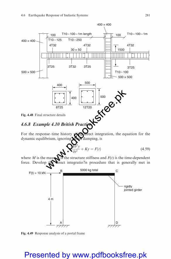
4.6.8 Example 4.10 British Practice
For the response–time history using direct integration, the equation for thedynamic equilibrium, ignoring initial damping, is
Md2ydt2
þ Ky ¼ FðtÞ (4:59)
where M is the mass, K is the structure stiffness and F(t) is the time-dependentforce. Develop the direct integratio7n procedure that is generally met in
100
4T32
3T25
400
8T25 12T20
400 500
500
3T32 3T25
4T32 4T32
3T25
T10 – 100 – 1m length
T10 – 125 T10 – 250
T10 – 100
500 × 500
500 × 500
400 × 400
T10 – 100 – 1m
400 × 400
30 × 50 1500
100
Fig. 4.48 Final structure details
4 m
F(t) = 10 kN5000 kg total CB
A D
rigidlyjointed girder
Fig. 4.49 Response analysis of a portal frame
4.6 Earthquake Response of Inelastic Systems 281
www.pdfbo
oksfr
ee.pk
Presented by www.pdfbooksfree.pk
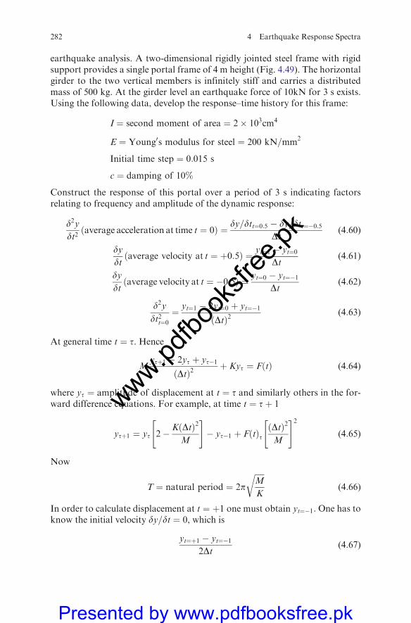
earthquake analysis. A two-dimensional rigidly jointed steel frame with rigidsupport provides a single portal frame of 4 m height (Fig. 4.49). The horizontalgirder to the two vertical members is infinitely stiff and carries a distributedmass of 500 kg. At the girder level an earthquake force of 10kN for 3 s exists.Using the following data, develop the response–time history for this frame:
I ¼ second moment of area ¼ 2� 103cm4
E ¼ Young0s modulus for steel ¼ 200 kN=mm2
Initial time step ¼ 0:015 s
c ¼ damping of 10%
Construct the response of this portal over a period of 3 s indicating factorsrelating to frequency and amplitude of the dynamic response:
d2ydt2ðaverage acceleration at time t ¼ 0Þ ¼ dy=dtt¼0:5 � dy=dtt¼�0:5
Dt(4:60)
dydtðaverage velocity at t ¼ þ0:5Þ ¼ yt¼1 � yt¼0
Dt(4:61)
dydtðaverage velocity at t ¼ �0:5Þ ¼ yt¼0 � yt¼�1
Dt(4:62)
d2ydt2t¼0
¼ yt¼1 � 2yt¼0 þ yt¼�1
ðDtÞ2(4:63)
At general time t ¼ t. Hence
Mytþ1 � 2yt þ yt�1
ðDtÞ2þ Kyt ¼ FðtÞ (4:64)
where yt ¼ amplitude of displacement at t ¼ t and similarly others in the for-ward difference equations. For example, at time t ¼ tþ 1
ytþ1 ¼ yt 2� KðDtÞ2
M
" #� yt�1 þ FðtÞt
ðDtÞ2
M
" #2(4:65)
Now
T ¼ natural period ¼ 2p
ffiffiffiffiffiM
K
r(4:66)
In order to calculate displacement at t ¼ þ1 one must obtain yt¼�1. One has toknow the initial velocity dy=dt ¼ 0, which is
yt¼þ1 � yt¼�12Dt
(4:67)
282 4 Earthquake Response Spectra
www.pdfbo
oksfr
ee.pk
Presented by www.pdfbooksfree.pk

or
yt¼�1 ¼ yt¼þ1 � 2Dtdy
dtt¼0(4:68)
The starting equation by making t� 0 becomes
y1 ¼ y02� KðDtÞ2
M
" #� y1 � 2Dt
dydt0
�þ FðtÞ0
ðDtÞ2
M
" #(4:69)
By including damping c ¼ 10%, i.e. cðdy=dtÞ in the generalized equation, then
Md2ydt2þ c
dydtþ Ky ¼ FðtÞ
Equation (4.69) becomes
ytþ1 1þ cDt2M
�¼ yt 2�KðDtÞ2
M
" #� yt�1 1� cDt
2M
�þ FðtÞt
ðDtÞ2
M
" #(4:70)
ytþ1 is computed from (4.70):
Kð2 columnsÞ ¼ 2� 12EI
L¼ 1:5� 106 Nm
T ¼ 2p
ffiffiffiffiffiM
K
r¼ 2p
ffiffiffiffiffiffiffiffiffiffiffiffiffiffiffiffiffiffiffi5000
1:5� 106
r¼ 0:3635 s
When c=10%, the maximum time-step interval = 0.036�0.04 s. The value ofDt ¼ 0:015s is acceptable. ytþ1 is given by
ytþ1 ¼ytð1:9325Þ � yt�1ð0:974Þ þ 4:5� 10�4FðtÞ
1:026
For the initial case
y1 ¼0þ 0þ 4:5� 10�4
2¼ 2:25� 10�4m
y2 ¼2:25� 10�4ð1:9325Þ � 0� 0:974þ 4:5� 10�4
1:026¼ 0:0008624m
y3 ¼0:0008624ð1:9325Þ � 2:25� 10�4 � 0:974þ 4:5� 10�4
1:026
¼ 0:0018493m
y4 ¼0:0018493� 1:9325� 0:0008624þ 4:5� 10�4
1:026¼ 0:0031198m
4.6 Earthquake Response of Inelastic Systems 283
www.pdfbo
oksfr
ee.pk
Presented by www.pdfbooksfree.pk
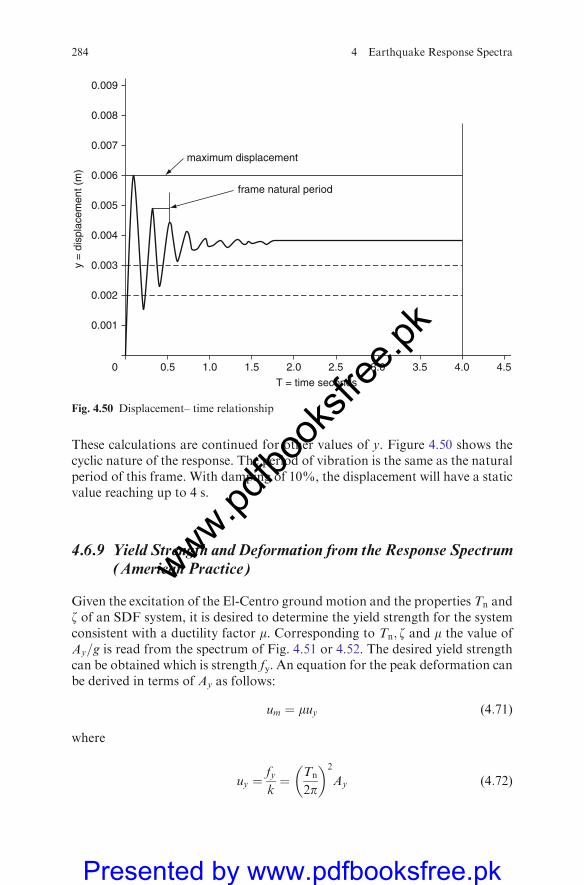
These calculations are continued for other values of y. Figure 4.50 shows thecyclic nature of the response. The period of vibration is the same as the naturalperiod of this frame. With damping of 10%, the displacement will have a staticvalue reaching up to 4 s.
4.6.9 Yield Strength and Deformation from the Response Spectrum(American Practice)
Given the excitation of the El-Centro ground motion and the properties Tn andz of an SDF system, it is desired to determine the yield strength for the systemconsistent with a ductility factor m. Corresponding to Tn; z and m the value ofAy=g is read from the spectrum of Fig. 4.51 or 4.52. The desired yield strengthcan be obtained which is strength fy. An equation for the peak deformation canbe derived in terms of Ay as follows:
um ¼ muy (4:71)
where
uy ¼fy
k¼ Tn
2p
� �2
Ay (4:72)
0.009
0.008
0.007maximum displacement
0.006frame natural period
0.005
y =
dis
plac
emen
t (m
)
T = time seconds
0.004
0.003
0.002
0.001
0 0.5 1.0 1.5 2.0 2.5 3.0 3.5 4.0 4.5
Fig. 4.50 Displacement– time relationship
284 4 Earthquake Response Spectra
www.pdfbo
oksfr
ee.pk
Presented by www.pdfbooksfree.pk
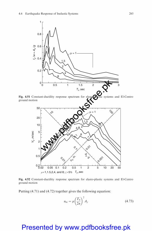
Putting (4.71) and (4.72) together gives the following equation:
um ¼ mTn
2p
� �2
Ay (4:73)
00 0.5
1.5
μ = 1
2
48
1 1.5 2 2.5 3
0.2
0.4
0.6
f y /w
= A
x /g
Tn .sec
0.8
1
Fig. 4.51 Constant-ductility response spectrum for elasto-plastic systems and El-Centroground motion
0.20.02 0.05
μ = 1,1.5,2,4, and 8; ζ = 5%
8
4 2
1.5
0.1
0.01
0.1
Ay , g
μ y, in
.
1
10
10010
1
0.1
0.01
0.00
1
μ = 1
0.2 0.5 1 2 5 10 20 50
1
0.5
2
10
5
Vy
,m/s
ec
Tn ,sec
20
50
Fig. 4.52 Constant-ductility response spectrum for elasto-plastic systems and El-Centroground motion
4.6 Earthquake Response of Inelastic Systems 285
www.pdfbo
oksfr
ee.pk
Presented by www.pdfbooksfree.pk
Example 4.11 American PracticeData Tn ¼ 0:5 sDamping z ¼ 5%Ductility m ¼ 4
Using Figs. 4.51 and 4.52 for the El-Centro ground motion, calculate the yieldstrength and deformation from the response spectrum or elasto-plastic systemshown in the figures.
Ay/g = 0.1789
fy ¼ the yield strength of an elasto-plastic system ¼ KUy ¼ mðw2nuyÞ
¼ mAy ¼ Ay=g ¼ 0:1789w
where w = weight of the systemA = pseudo-acceleration response spectrum for linearly elastic systems
Uy ¼fy
k
Tn
2p
� �2
Ay ¼0:5
2p
� �2
f0:179 gg g ¼ 386
¼ 0:437 inð11:1 mmÞ
Um ¼ 4� 0:437 � 1:749 inð44:5 mmÞ
4.7 Equivalent Static Force Method Based on Eurocode-8
4.7.1 General Introduction
Equivalent static response spectrum method and time history method areaccepted by EC8 in order to evaluate seismic forces while treating at the sametime the building which is symmetrical in elevation and plan.
One of the plan frame is taken as an example and shall be assumed moment-resisting rigid frame.
4.7.2 Evaluation of Lumped Masses to Various Floor Levels
Step 1 Lumped mass evaluation
(a) Roof: Mass of infill + mass of columns + mass of beams longitudinallyand transversely of the floor + mass of slab + imposed load or action onroof wherever possible
(b) Mass of floor: Masses of all floors: seismic weight of each floor = full deadload + imposed load. Any weight supported between storeys
(c) Imposed loads or actions(d) Total seismic weight of the building: m ¼ m1 þm2 þm3 þ
286 4 Earthquake Response Spectra
www.pdfbo
oksfr
ee.pk
Presented by www.pdfbooksfree.pk
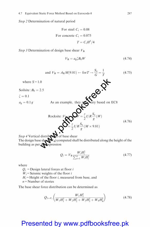
Step 2 Determination of natural period
For steel Ct ¼ 0:08
For concrete Ct ¼ 0:075
T ¼ CtH3=4
Step 3 Determination of design base shear VB
VB ¼ agzB0W (4:74)
and VB ¼ ARMð9:81Þ forT! Sa
G¼ 1
T(4:75)
where S=1.0
Soilsite :B0 ¼ 2:5
z ¼ 0:1
ag ¼ 0:1 g As an example; they may vary based on EC8
Rocksite :VB ¼ ARW ¼z
2I=R
Sa
gðWÞ
¼ z
2I=R
Sa
gðM� 9:81Þ
(4:76)
Step 4 Vertical distribution of base shearThe design base shear (VB) computed shall be distributed along the height of thebuilding as per the expression
Qi ¼ VBWiH
2iPn
i¼1 WiH2i
(4:77)
whereQi =Design lateral forces at floor iWi=Seismic weights of the floor iHi=Height of the floor i, measured from base, andn=Number of stories
The base shear force distribution can be determined as
Q1¼V1
W1H21
W1H21 þW2H
22 þW3H
23 þW4H
24
� �(4:78)
4.7 Equivalent Static Force Method Based on Eurocode-8 287
www.pdfbo
oksfr
ee.pk
Presented by www.pdfbooksfree.pk

4.7.3 Response Spectrum Method
A: Frame without considering the stiffness of infillsA step-by-step procedure for analysis of the frame by response spectrummethod is as follows.
4.7.3.1 Step 1: Determination of Eigenvalues and Eigenvectors
Mass matrix,M, and stiffness matrix,K, of the plane frame lumped mass modelare
½M� ¼
M1 0 0 0
0 M2 0 0
0 0 M3 0
0 0 0 M4
26664
37775n�n
(4:79)
Note: The terms in a matrix can be of n � n terms (n = 4 as an example)Column Stiffness of Storey
K ¼ 12EI
L3(4:80)
The lateral stiffness of each storey
k1; k2; k3; . . . ; kn (4:81)
Stiffness of lumped mass modelled as
k ¼
k1 þ k1 �k2 0 0
�k2 k2 þ k3 �k3 0
0 �k3 k3 þ k4 �k40 0 �k4 k4
26664
37775 (4:82)
n = 4 for a caseThe stiffness, mass matrices, eigenvalues and eigenvectors are
jK� o2mj ¼
2 k� o2M �k2 0 0
�k2 2 k� o2M �k3 0
0 �k2 2 k� o2M �k30 0 �k4 k� o20:575M
���������
���������n�n
(4:83)
= 0
288 4 Earthquake Response Spectra
www.pdfbo
oksfr
ee.pk
Presented by www.pdfbooksfree.pk
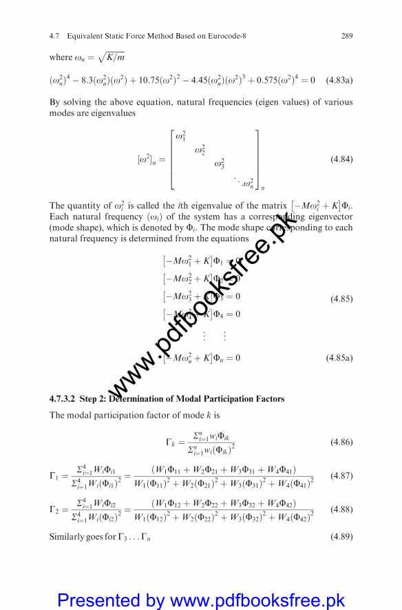
where on ¼ffiffiffiffiffiffiffiffiffiffiK=m
p
ðo2nÞ
4 � 8:3ðo2nÞðo2Þ þ 10:75ðo2Þ2 � 4:45ðo2
nÞðo2Þ3 þ 0:575ðo2Þ4 ¼ 0 (4:83a)
By solving the above equation, natural frequencies (eigen values) of variousmodes are eigenvalues
½o2�n ¼
o21
o22
o23
. ..
o2n
2666664
3777775n
(4:84)
The quantity of o2i is called the ith eigenvalue of the matrix �Mo2
i þ K�
Fi.Each natural frequency ðoiÞ of the system has a corresponding eigenvector(mode shape), which is denoted by Fi. The mode shape corresponding to eachnatural frequency is determined from the equations
�Mo21 þ K
� F1 ¼ 0
�Mo22 þ K
� F2 ¼ 0
�Mo23 þ K
� F3 ¼ 0
�Mo24 þ K
� F4 ¼ 0
..
. ...
(4:85)
�Mo2n þ K
� Fn ¼ 0 (4:85a)
4.7.3.2 Step 2: Determination of Modal Participation Factors
The modal participation factor of mode k is
Gk ¼Sni¼1wiFik
Sni¼1wiðFikÞ2
(4:86)
G1 ¼S4i¼1WiFi1
S4i¼1WiðFi1Þ2
¼ ðW1F11 þW2F21 þW3F31 þW4F41ÞW1ðF11Þ2 þW2ðF21Þ2 þW3ðF31Þ2 þW4ðF41Þ2
(4:87)
G2 ¼S4i¼1WiFi2
S4i¼1WiðFi2Þ2
¼ ðW1F12 þW2F22 þW3F32 þW4F42ÞW1ðF12Þ2 þW2ðF22Þ2 þW3ðF32Þ2 þW4ðF42Þ2
(4:88)
Similarly goes forG3 . . .Gn (4:89)
4.7 Equivalent Static Force Method Based on Eurocode-8 289
www.pdfbo
oksfr
ee.pk
Presented by www.pdfbooksfree.pk

whereg = Acceleration due to gravity,Fik ¼Mode shape coefficient at floor i in mode k, andWi = Seismic weight of floor i.
4.7.3.3 Step 3: Modal Masses
M1 ¼S4i¼1WiFi1
� 2g S4
i¼1WiðFi1Þ2h i (4:90)
Similarly for others up to nth mass Mn
Modal contributions of various modes
Formodel 1 ¼M1
M
..
.
For model n ¼Mn
M
(4:91)
4.7.3.4 Step 4: Determination of Lateral Force at Each Floor in Each Mode
Qik = design lateral force at floor ‘‘i’’ in mode ‘‘k’’ is given by
AkFikGkWi (4:92)
where Ak = design horizontal acceleration spectrum value using the naturalperiod of vibration ‘‘Tk’’ of mode ‘‘k’’
The design horizontal seismic coefficient for various modes are
ARk ¼Z
2
I
R
Sak
gif it is rock (4:93)
Or if soil: agSzB0
4.7.3.5 Step 5: Determination of Storey Shear Forces in Each Mode
The peak shear force is given by
Vik ¼Xnl¼iþ1
Qlk (4:94)
4.7.3.6 Step 6: Determination of Storey Shear Force due to All Modes
The peak shear force Vi in storey ‘‘i’’ due to all modes is obtained by combiningthose due to each mode in accordance with
290 4 Earthquake Response Spectra
www.pdfbo
oksfr
ee.pk
Presented by www.pdfbooksfree.pk
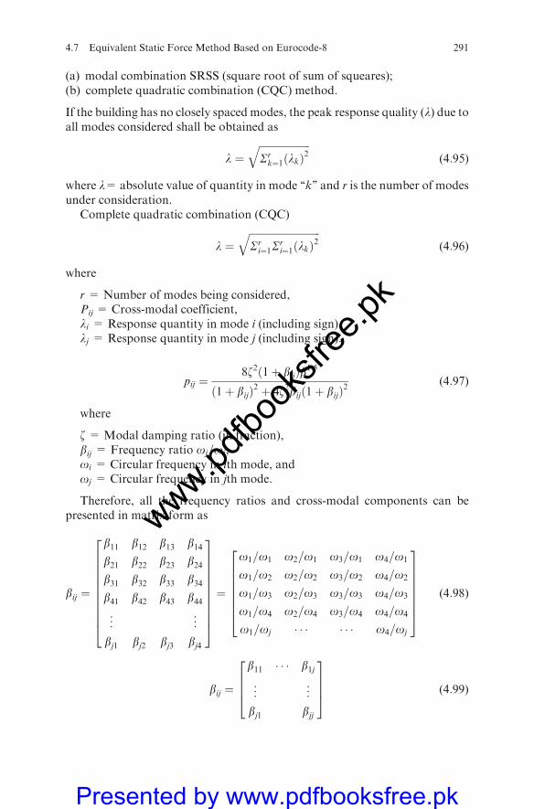
(a) modal combination SRSS (square root of sum of squeares);(b) complete quadratic combination (CQC) method.
If the building has no closely spaced modes, the peak response quality (l) due toall modes considered shall be obtained as
l ¼ffiffiffiffiffiffiffiffiffiffiffiffiffiffiffiffiffiffiffiffiSrk¼1ðlkÞ
2q
(4:95)
where l=absolute value of quantity in mode ‘‘k’’ and r is the number of modesunder consideration.
Complete quadratic combination (CQC)
l ¼ffiffiffiffiffiffiffiffiffiffiffiffiffiffiffiffiffiffiffiffiffiffiffiffiffiffiffiffiSri¼1S
ri¼1ðlkÞ
2q
(4:96)
where
r = Number of modes being considered,Pij = Cross-modal coefficient,li = Response quantity in mode i (including sign),lj = Response quantity in mode j (including sign).
pij ¼8z2ð1þ bijÞb1:5
ð1þ bijÞ2 þ 4z2bijð1þ bijÞ2(4:97)
where
z = Modal damping ratio (in fraction),bij = Frequency ratio oj=oi,oi = Circular frequency in ith mode, andoj = Circular frequency in jth mode.
Therefore, all the frequency ratios and cross-modal components can bepresented in matrix form as
bij ¼
b11 b12 b13 b14b21 b22 b23 b24b31 b32 b33 b34b41 b42 b43 b44
..
. ...
bj1 bj2 bj3 bj4
26666666664
37777777775¼
o1=o1 o2=o1 o3=o1 o4=o1
o1=o2 o2=o2 o3=o2 o4=o2
o1=o3 o2=o3 o3=o3 o4=o3
o1=o4 o2=o4 o3=o4 o4=o4
o1=oj o4=oj
26666664
37777775
(4:98)
bij ¼
b11 b1j
..
. ...
bj1 bjj
2664
3775 (4:99)
4.7 Equivalent Static Force Method Based on Eurocode-8 291
www.pdfbo
oksfr
ee.pk
Presented by www.pdfbooksfree.pk
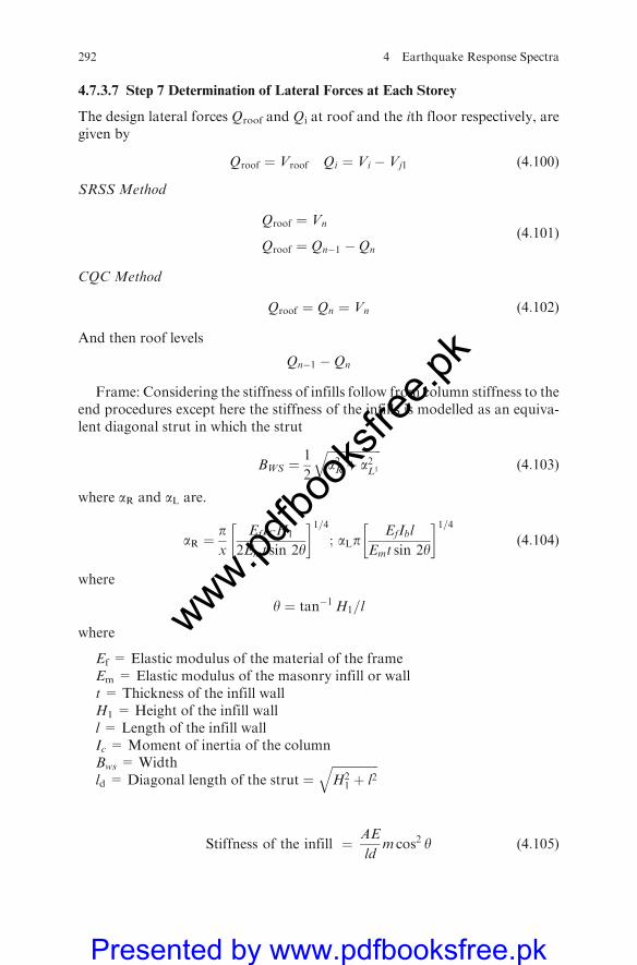
4.7.3.7 Step 7 Determination of Lateral Forces at Each Storey
The design lateral forces Qroof and Qi at roof and the ith floor respectively, aregiven by
Qroof ¼ Vroof Qi ¼ Vi � Vj1 (4:100)
SRSS Method
Qroof ¼ Vn
Qroof ¼ Qn�1 �Qn
(4:101)
CQC Method
Qroof ¼ Qn ¼ Vn (4:102)
And then roof levels
Qn�1 �Qn
Frame: Considering the stiffness of infills follow from column stiffness to theend procedures except here the stiffness of the infills is modelled as an equiva-lent diagonal strut in which the strut
BWS ¼1
2
ffiffiffiffiffiffiffiffiffiffiffiffiffiffiffiffiffiffia2R þ a2
L1
q(4:103)
where aR and aL are.
aR ¼px
EfICH1
2Emt sin 2y
�1=4; aLp
EfIbl
Emt sin 2y
�1=4(4:104)
where
y ¼ tan�1 H1=l
where
Ef = Elastic modulus of the material of the frameEm = Elastic modulus of the masonry infill or wallt = Thickness of the infill wallH1 = Height of the infill walll = Length of the infill wallIc = Moment of inertia of the columnBws = Widthld = Diagonal length of the strut ¼
ffiffiffiffiffiffiffiffiffiffiffiffiffiffiffiH2
1 þ l2q
Stiffness of the infill ¼ AE
ldm cos2 y (4:105)
292 4 Earthquake Response Spectra
www.pdfbo
oksfr
ee.pk
Presented by www.pdfbooksfree.pk
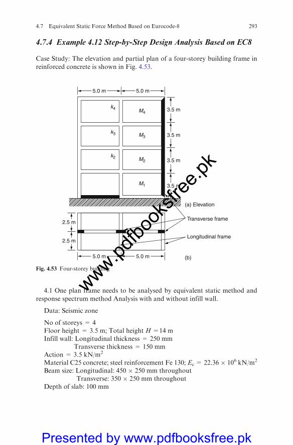
4.7.4 Example 4.12 Step-by-Step Design Analysis Based on EC8
Case Study: The elevation and partial plan of a four-storey building frame in
reinforced concrete is shown in Fig. 4.53.
4.1 One plan frame needs to be analysed by equivalent static method and
response spectrum method Analysis with and without infill wall.
Data: Seismic zone
No of storeys = 4Floor height = 3.5 m; Total height H =14 mInfill wall: Longitudinal thickness = 250 mm
Transverse thickness = 150 mmAction = 3.5 kN/m2
Material C25 concrete; steel reinforcement Fe 130; Ec = 22.36 � 106 kN/m2
Beam size: Longitudinal: 450 � 250 mm throughoutTransverse: 350 � 250 mm throughout
Depth of slab: 100 mm
5.0 m
3.5 m
3.5 m
5.0 m
k4
k3
k2
M4
M3
M2
M1
3.5 m
3.5 m
2.5 m
2.5 m
5.0 m 5.0 m
(a) Elevation
Transverse frame
Longitudinal frame
(b)
Fig. 4.53 Four-storey building
4.7 Equivalent Static Force Method Based on Eurocode-8 293
www.pdfbo
oksfr
ee.pk
Presented by www.pdfbooksfree.pk
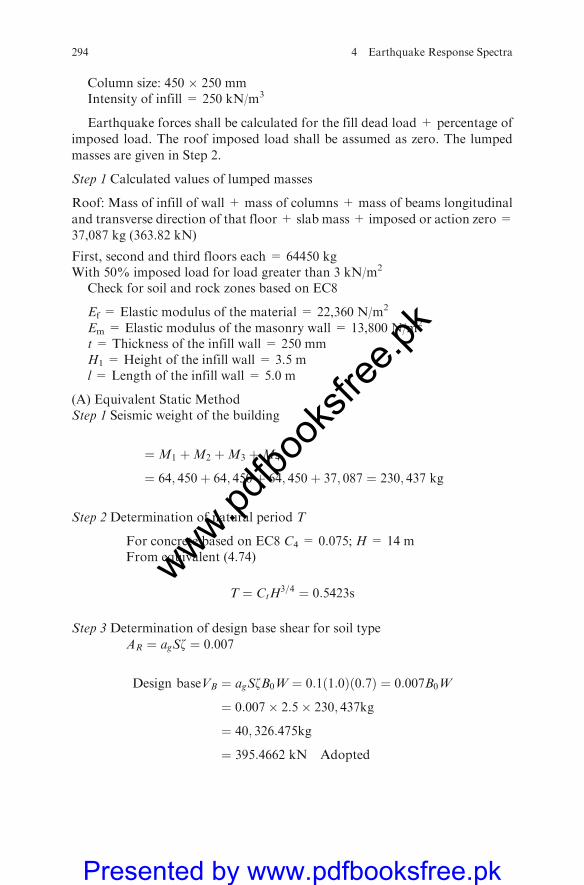
Column size: 450 � 250 mmIntensity of infill = 250 kN/m3
Earthquake forces shall be calculated for the fill dead load + percentage ofimposed load. The roof imposed load shall be assumed as zero. The lumped
masses are given in Step 2.
Step 1 Calculated values of lumped masses
Roof: Mass of infill of wall + mass of columns + mass of beams longitudinal
and transverse direction of that floor + slab mass + imposed or action zero =37,087 kg (363.82 kN)
First, second and third floors each = 64450 kgWith 50% imposed load for load greater than 3 kN/m2
Check for soil and rock zones based on EC8
Ef = Elastic modulus of the material = 22,360 N/m2
Em = Elastic modulus of the masonry wall = 13,800 N/m2
t = Thickness of the infill wall = 250 mmH1 = Height of the infill wall = 3.5 ml = Length of the infill wall = 5.0 m
(A) Equivalent Static MethodStep 1 Seismic weight of the building
¼M1 þM2 þM3 þM4
¼ 64; 450þ 64; 450þ 64; 450þ 37; 087 ¼ 230; 437 kg
Step 2 Determination of natural period T
For concrete based on EC8 C4 = 0.075; H = 14 mFrom equivalent (4.74)
T ¼ CtH3=4 ¼ 0:5423s
Step 3 Determination of design base shear for soil type
AR ¼ agSz ¼ 0:007
Design baseVB ¼ agSzB0W ¼ 0:1ð1:0Þð0:7Þ ¼ 0:007B0W
¼ 0:007� 2:5� 230; 437kg
¼ 40; 326:475kg
¼ 395:4662 kN Adopted
294 4 Earthquake Response Spectra
www.pdfbo
oksfr
ee.pk
Presented by www.pdfbooksfree.pk
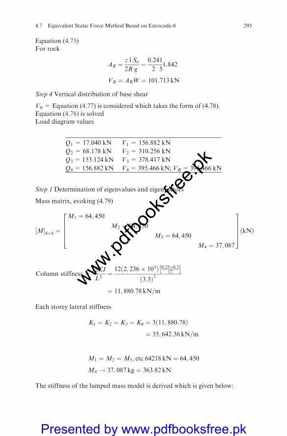
Equation (4.75)For rock
AR ¼z
2
1
R
Sa
g¼ 0:24
2
1
51:842
VB ¼ ARW ¼ 101:713 kN
Step 4 Vertical distribution of base shear
V0 = Equation (4.77) is considered which takes the form of (4.78).Equation (4.78) is solvedLoad diagram values
Q1 = 17.040 kN V1 = 156.882 kN
Q2 = 68.178 kN V2 = 310.256 kN
Q3 = 153.124 kN V3 = 378.417 kN
Q4 = 156.882 kN V4 = 395.466 kN; VB=395.466 kN
Step 1 Determination of eigenvalues and eigenvectors
Mass matrix, evoking (4.79)
½M�4�4 ¼
M1 ¼ 64; 450
M2 ¼ 64; 450
M3 ¼ 64; 450
M4 ¼ 37; 087
26664
37775ðkNÞ
Column stiffness ¼ 12EJ
L3¼
12ð2; 236� 103Þ 0:25�0:312
� ð3:5Þ3
¼ 11; 880:78 kN=m
Each storey lateral stiffness
K1 ¼ K2 ¼ K3 ¼ K4 ¼ 3ð11; 880:78Þ
¼ 35; 642:36 kN=m
M1 ¼M2 ¼M3; etc:64218 kN ¼ 64; 450
M4 ! 37; 087 kg ¼ 363:82 kN
The stiffness of the lumped mass model is derived which is given below:
4.7 Equivalent Static Force Method Based on Eurocode-8 295
www.pdfbo
oksfr
ee.pk
Presented by www.pdfbooksfree.pk
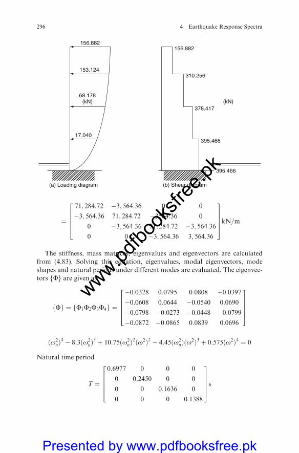
¼
71; 284:72 �3; 564:36 0 0
�3; 564:36 71; 284:72 �3564:36 0
0 �3; 564:36 71; 284:72 �3; 564:360 0 �3; 564:36 3; 564:36
26664
37775kN=m
The stiffness, mass matrices, eigenvalues and eigenvectors are calculatedfrom (4.83). Solving this equation, eigenvalues, modal eigenvectors, modeshapes and natural periods under different modes are evaluated. The eigenvec-tors Ff g are given as
Ff g ¼ F1F2F3F4f g ¼
�0:0328 0:0795 0:0808 �0:0397�0:0608 0:0644 �0:0540 0:0690
�0:0798 �0:0273 �0:0448 �0:0799�0:0872 �0:0865 0:0839 0:0696
26664
37775
ðo2nÞ
4 � 8:3ðo2nÞ
3 þ 10:75ðo2nÞ
2ðo2Þ2 � 4:45ðo2nÞðo2Þ3 þ 0:575ðo2Þ4 ¼ 0
Natural time period
T ¼
0:6977 0 0 0
0 0:2450 0 0
0 0 0:1636 0
0 0 0 0:1388
26664
37775s
153.124
156.882156.882
310.256
378.417
395.466
395.466
68.178(kN) (kN)
17.040
(a) Loading diagram (b) Shear diagram
296 4 Earthquake Response Spectra
www.pdfbo
oksfr
ee.pk
Presented by www.pdfbooksfree.pk
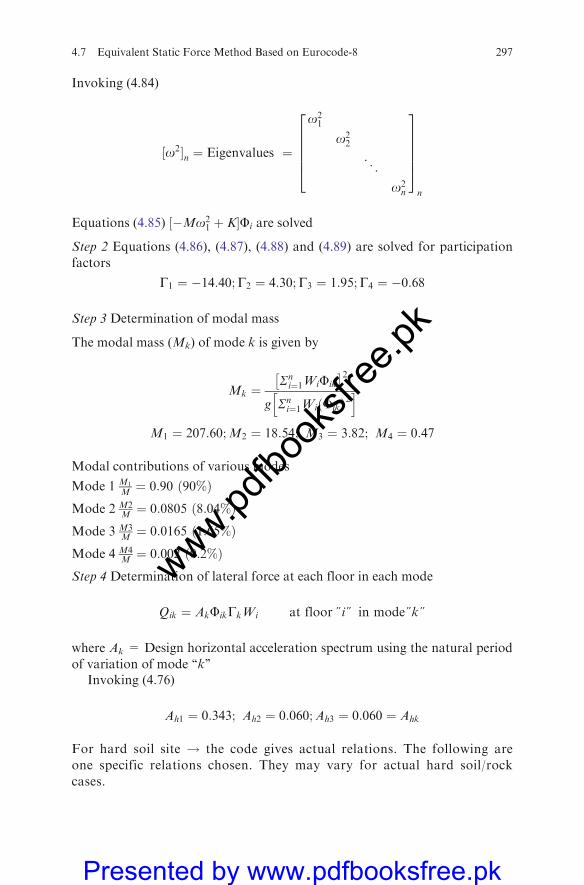
Invoking (4.84)
½o2�n ¼ Eigenvalues ¼
o21
o22
. ..
o2n
266664
377775n
Equations (4.85) ½�Mo21 þ K�Fi are solved
Step 2 Equations (4.86), (4.87), (4.88) and (4.89) are solved for participation
factors
G1 ¼ �14:40;G2 ¼ 4:30;G3 ¼ 1:95;G4 ¼ �0:68
Step 3 Determination of modal mass
The modal mass (Mk) of mode k is given by
Mk ¼Sni¼1WiFik
� 2g Sn
i¼1WiðFikÞ2h i
M1 ¼ 207:60;M2 ¼ 18:54; M3 ¼ 3:82; M4 ¼ 0:47
Modal contributions of various modes
Mode 1 M1
M ¼ 0:90 ð90%ÞMode 2 M2
M ¼ 0:0805 ð8:04%ÞMode 3 M3
M¼ 0:0165 ð1:65%Þ
Mode 4 M4M ¼ 0:002 ð0:2%Þ
Step 4 Determination of lateral force at each floor in each mode
Qik ¼ AkFikGkWi at floor }i} in mode}k}
where Ak = Design horizontal acceleration spectrum using the natural period
of variation of mode ‘‘k’’Invoking (4.76)
Ah1 ¼ 0:343; Ah2 ¼ 0:060;Ah3 ¼ 0:060 ¼ Ahk
For hard soil site ! the code gives actual relations. The following are
one specific relations chosen. They may vary for actual hard soil/rock
cases.
4.7 Equivalent Static Force Method Based on Eurocode-8 297
www.pdfbo
oksfr
ee.pk
Presented by www.pdfbooksfree.pk
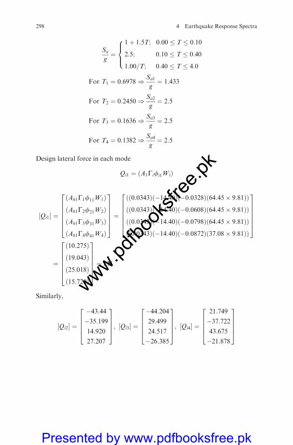
Sa
g¼
1þ 1:5T; 0:00 � T � 0:10
2:5; 0:10 � T � 0:40
1:00=T; 0:40 � T � 4:0
8><>:
For T1 ¼ 0:6978) Sa1
g¼ 1:433
For T2 ¼ 0:2450) Sa2
g¼ 2:5
For T3 ¼ 0:1636) Sa3
g¼ 2:5
For T4 ¼ 0:1382) Sa4
g¼ 2:5
Design lateral force in each mode
Qi1 ¼ ðA1Gifi1WiÞ
½Qi1� ¼
ðAh1G1f11W1Þ
ðAh1G2f21W2Þ
ðAh1G3f31W3Þ
ðAh1G4f41W4Þ
2666664
3777775¼
ðð0:0343Þð�14:40Þð�0:0328Þð64:45� 9:81ÞÞ
ðð0:0343Þð�14:40Þð�0:0608Þð64:45� 9:81ÞÞ
ðð0:0343Þð�14:40Þð�0:0798Þð64:45� 9:81ÞÞ
ðð0:0343Þð�14:40Þð�0:0872Þð37:08� 9:81ÞÞ
2666664
3777775
¼
ð10:275Þ
ð19:043Þ
ð25:018Þ
ð15:720Þ
2666664
3777775¼ kN
Similarly,
½Qi2� ¼
�43:44�35:19914:920
27:207
26664
37775; ½Qi3� ¼
�44:20429:499
24:517
�26:385
26664
37775; ½Qi4� ¼
21:749
�37:72243:675
�21:878
26664
37775
298 4 Earthquake Response Spectra
www.pdfbo
oksfr
ee.pk
Presented by www.pdfbooksfree.pk
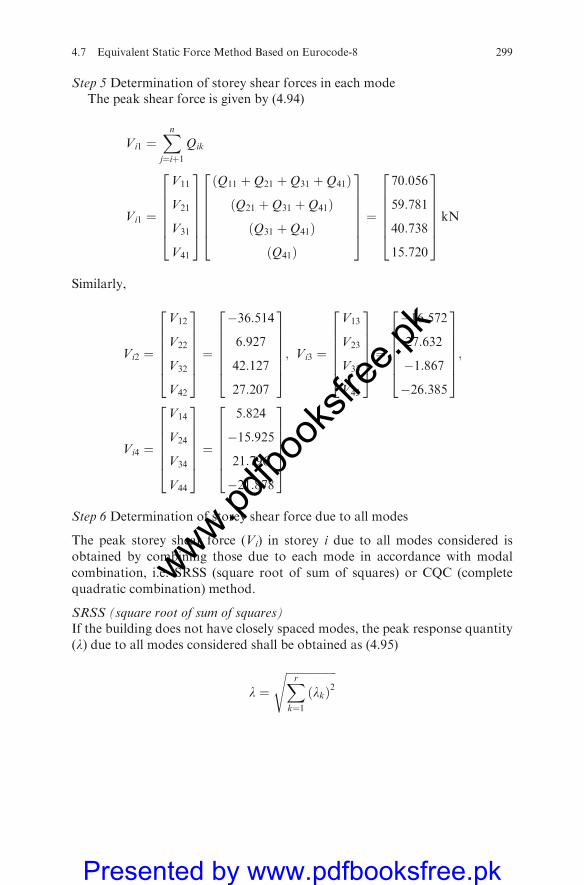
Step 5 Determination of storey shear forces in each modeThe peak shear force is given by (4.94)
Vi1 ¼Xnj¼iþ1
Qik
Vi1 ¼
V11
V21
V31
V41
2666664
3777775
Q11 þQ21 þQ31 þQ41ð Þ
Q21 þQ31 þQ41ð Þ
Q31 þQ41ð Þ
Q41ð Þ
2666664
3777775¼
70:056
59:781
40:738
15:720
2666664
3777775kN
Similarly,
Vi2 ¼
V12
V22
V32
V42
2666664
3777775¼
�36:514
6:927
42:127
27:207
2666664
3777775; Vi3 ¼
V13
V23
V33
V43
2666664
3777775¼
�16:572
27:632
�1:867
�26:385
2666664
3777775;
Vi4 ¼
V14
V24
V34
V44
2666664
3777775¼
5:824
�15:925
21:796
�21:878
2666664
3777775
Step 6 Determination of storey shear force due to all modes
The peak storey shear force (Vi) in storey i due to all modes considered isobtained by combining those due to each mode in accordance with modal
combination, i.e. SRSS (square root of sum of squares) or CQC (completequadratic combination) method.
SRSS (square root of sum of squares)If the building does not have closely spaced modes, the peak response quantity(l) due to all modes considered shall be obtained as (4.95)
l ¼ffiffiffiffiffiffiffiffiffiffiffiffiffiffiffiffiffiffiXrk¼1
lkð Þ2s
4.7 Equivalent Static Force Method Based on Eurocode-8 299
www.pdfbo
oksfr
ee.pk
Presented by www.pdfbooksfree.pk
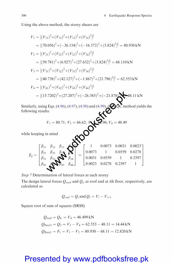
Using the above method, the storey shears are
V1 ¼ ½ V11ð Þ2þ V12ð Þ2þ V13ð Þ2þ V14ð Þ2�12
¼ ½ 70:056ð Þ2þ �36:154ð Þ2þ �16:572ð Þ2þ 5:824ð Þ2�12 ¼ 80:930 kN
V2 ¼ ½ V21ð Þ2þ V22ð Þ2þ V23ð Þ2þ V24ð Þ2�12
¼ ½ 59:781ð Þ2þ 6:927ð Þ2þ 27:632ð Þ2þ 5:824ð Þ2�12 ¼ 68:110 kN
V3 ¼ ½ V31ð Þ2þ V32ð Þ2þ V33ð Þ2þ V34ð Þ2�12
¼ ½ 40:738ð Þ2þ 42:127ð Þ2þ �1:867ð Þ2þ 21:796ð Þ2�12 ¼ 62:553 kN
V4 ¼ ½ V41ð Þ2þ V42ð Þ2þ V43ð Þ2þ V44ð Þ2�12
¼ ½ 15:7202ð Þ2þ 27:207ð Þ2þ �26:385ð Þ2þ �21:878ð Þ2�12 ¼ 48:11 kN
Similarly, using Eqs. (4.96), (4.97), (4.98) and (4.99), the CQCmethod yields thefollowing results:
V1 ¼ 80:71; V2 ¼ 66:62; V3 ¼ 62:96;V4 ¼ 48:49
while keeping in mind
bij ¼
b11 b12 b13 b14b21 b22 b23 b24b31 b32 b33 b34b41 b42 b43 b44
26664
37775 ¼
1 0:0073 0:0031 0:0023
0:0073 1 0:0559 0:0278
0:0031 0:0559 1 0:2597
0:0023 0:0278 0:2597 1
26664
37775
Step 7 Determination of lateral forces at each storey
The design lateral forces Qroof and Qi, at roof and at ith floor, respectively, arecalculated as
Qroof ¼ Qi andQi ¼ Vi � Viþ1
Square root of sum of squares (SRSS)
Qroof ¼ Q4 ¼ V4 ¼ 46:499 kN
Qfloor3 ¼ Q3 ¼ V3 � V4 ¼ 62:553� 48:11 ¼ 14:44 kN
Qfloor1 ¼ F1 ¼ V1 � V2 ¼ 80:930� 68:11 ¼ 12:820 kN
300 4 Earthquake Response Spectra
www.pdfbo
oksfr
ee.pk
Presented by www.pdfbooksfree.pk
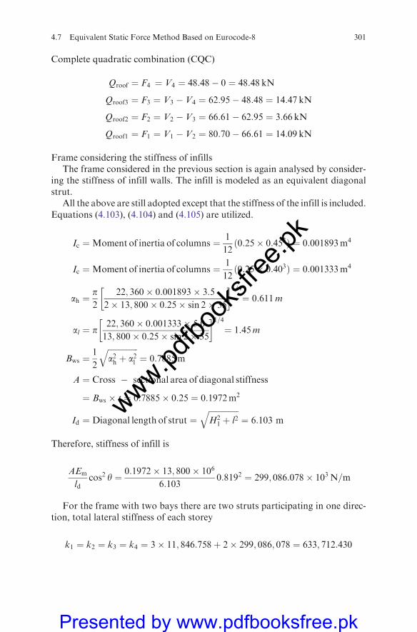
Complete quadratic combination (CQC)
Qroof ¼ F4 ¼ V4 ¼ 48:48� 0 ¼ 48:48 kN
Qroof3 ¼ F3 ¼ V3 � V4 ¼ 62:95� 48:48 ¼ 14:47 kN
Qroof2 ¼ F2 ¼ V2 � V3 ¼ 66:61� 62:95 ¼ 3:66 kN
Qroof1 ¼ F1 ¼ V1 � V2 ¼ 80:70� 66:61 ¼ 14:09 kN
Frame considering the stiffness of infillsThe frame considered in the previous section is again analysed by consider-
ing the stiffness of infill walls. The infill is modeled as an equivalent diagonalstrut.
All the above are still adopted except that the stiffness of the infill is included.Equations (4.103), (4.104) and (4.105) are utilized.
Ic ¼Moment of inertia of columns ¼ 1
12ð0:25� 0:453Þ ¼ 0:001893m4
Ic ¼Moment of inertia of columns ¼ 1
12ð0:25� 0:403Þ ¼ 0:001333m4
ah ¼p2
22; 360� 0:001893� 3:5
2� 13; 800� 0:25� sin 2� 35
�1=4¼ 0:611m
al ¼ p22; 360� 0:001333� 5:0
13; 800� 0:25� sin 2� 35
�1=4¼ 1:45m
Bws ¼1
2
ffiffiffiffiffiffiffiffiffiffiffiffiffiffiffia2h þ a2l
q¼ 0:7885m
A ¼ Cross � sectional area of diagonal stiffness
¼ Bws � t ¼ 0:7885� 0:25 ¼ 0:1972m2
Id ¼ Diagonal length of strut ¼ffiffiffiffiffiffiffiffiffiffiffiffiffiffiffiH2
1 þ l2q
¼ 6:103 m
Therefore, stiffness of infill is
AEm
ldcos2 y ¼ 0:1972� 13; 800� 106
6:1030:8192 ¼ 299; 086:078� 103 N=m
For the frame with two bays there are two struts participating in one direc-tion, total lateral stiffness of each storey
k1 ¼ k2 ¼ k3 ¼ k4 ¼ 3� 11; 846:758þ 2� 299; 086; 078 ¼ 633; 712:430
4.7 Equivalent Static Force Method Based on Eurocode-8 301
www.pdfbo
oksfr
ee.pk
Presented by www.pdfbooksfree.pk
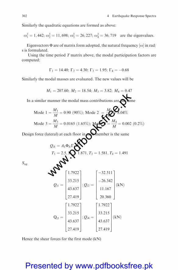
Similarly the quadratic equations are formed as above:
o21 ¼ 1; 442; o2
2 ¼ 11; 698; o23 ¼ 26; 227; o2
4 ¼ 36; 719 are the eigenvalues:
EigenvectorsF are of matrix form adopted, the natural frequency ½o� in rad/s is formulated.
Using the time period T matrix above, the modal participation factors arecomputed:
G1 ¼ 14:40; G2 ¼ 4:30; G3 ¼ 1:95; G4 ¼ �0:68
Similarly the modal masses are evaluated. The new values will be
M1 ¼ 207:60; M2 ¼ 18:54; M3 ¼ 3:82; M4 ¼ 0:47
In a similar manner the modal mass contributions are the same
Mode 1 ¼M1
M¼ 0:90 ð90%Þ; Mode 2 ¼ M2
M¼ 8:04%
Mode 3 ¼M3
M¼ 0:0165 ð1:65%Þ; Mode 4 ¼M4
M¼ 0:002 ð0:2%Þ
Design force (lateral) at each floor in each member is the same
Qik ¼ AkFikGkWi
T1 ¼ 2:5;T2 ¼ 1:871;T3 ¼ 1:581;T4 ¼ 1:491
Sag
Qi1 ¼
1:7922
33:215
43:637
27:419
26666664
37777775
;Qi2 ¼
�32:511
�26:342
11:167
20:360
26666664
37777775ðkNÞ
Qi3 ¼
1:7922
33:215
43:637
27:419
26666664
37777775
;Qi4 ¼
1:7922
33:215
43:637
27:419
26666664
37777775ðkNÞ
Hence the shear forces for the first mode (kN)
302 4 Earthquake Response Spectra
www.pdfbo
oksfr
ee.pk
Presented by www.pdfbooksfree.pk
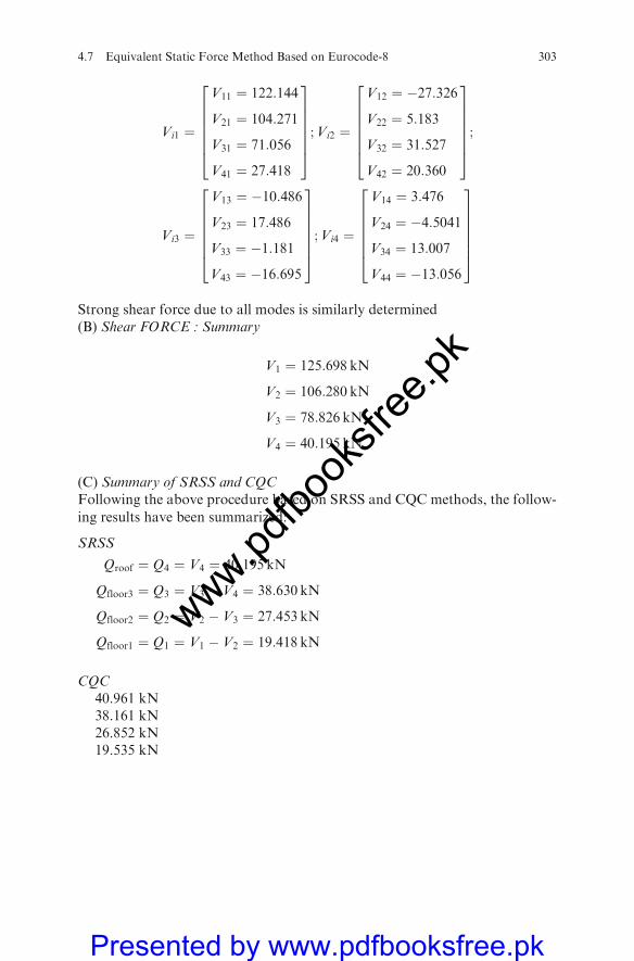
Vi1 ¼
V11 ¼ 122:144
V21 ¼ 104:271
V31 ¼ 71:056
V41 ¼ 27:418
2666664
3777775
;Vi2 ¼
V12 ¼ �27:326
V22 ¼ 5:183
V32 ¼ 31:527
V42 ¼ 20:360
2666664
3777775
;
Vi3 ¼
V13 ¼ �10:486
V23 ¼ 17:486
V33 ¼ �1:181
V43 ¼ �16:695
2666664
3777775
;Vi4 ¼
V14 ¼ 3:476
V24 ¼ �4:5041
V34 ¼ 13:007
V44 ¼ �13:056
2666664
3777775
Strong shear force due to all modes is similarly determined(B) Shear FORCE : Summary
V1 ¼ 125:698 kN
V2 ¼ 106:280 kN
V3 ¼ 78:826 kN
V4 ¼ 40:195 kN
(C) Summary of SRSS and CQCFollowing the above procedure based on SRSS and CQC methods, the follow-
ing results have been summarized:
SRSS
Qroof ¼ Q4 ¼ V4 ¼ 40:195 kN
Qfloor3 ¼ Q3 ¼ V3 � V4 ¼ 38:630 kN
Qfloor2 ¼ Q2 ¼ V2 � V3 ¼ 27:453 kN
Qfloor1 ¼ Q1 ¼ V1 � V2 ¼ 19:418 kN
CQC40.961 kN38.161 kN26.852 kN19.535 kN
4.7 Equivalent Static Force Method Based on Eurocode-8 303
www.pdfbo
oksfr
ee.pk
Presented by www.pdfbooksfree.pk

www.pdfbo
oksfr
ee.pk
Presented by www.pdfbooksfree.pk
Chapter 5
Dynamic Finite Element Analysis of Structures
5.1 Introduction
Because of the large number of computer runs required for dynamic analysis, it isvery important that accurate and numerically efficient methods be used withincomputer programs. These methods have been described adequately. Equationof motion for various structures with seismic devices is given. Their functions areidentified when various solution procedures are used. Some of the solutionprocedures popularly adopted by various resea rches are explained. A completefinite element procedure is given which can easily be linked to typical dynamicanalysis chosen for a specific case study. These analyses are generally adopted bymany well-known finite element computer packages. The analysis given has theflexibility to be adopted in any new package in the offing. Computer subroutinescan be developed to link the main finite element analysis package with theperformance of specific seismic devices. Many computerized finite elementpackages have such facilities. The purpose of this chapter is to give credit to thepower of finite element in the use of earthquake-resistant structures.
Part A: Analysis with solution proceduresDynamic Elastic Analysis with and without Seismic Devices
5.2 Dynamic Equilibrium
5.2.1 Lumped Mass system
The force equilibrium of a multi-degree-of-freedom lumped mass system as afunction of time can be expressed by the following equation:
fðtÞ1 þ fðtÞD þ fðtÞs ¼ fðtÞ (5:1)
in which the force vectors at time t are
f ðtÞ1 is a vector of inertia forces acting on the node massesf ðtÞD is a vector of viscous damping forces
M.Y.H. Bangash, Earthquake Resistant Buildings,DOI 10.1007/978-3-540-93818-7_5, � M.Y.H. Bangash 2011
305
www.pdfbo
oksfr
ee.pk
Presented by www.pdfbooksfree.pk
f ðtÞS is a vector of forces carried by the structuref ðtÞ is a vector of externally applied loads
Equation (5.1) is valid for both linear and non-linear systems if equilibrium isformulated with respect to the deformed geometry of the structure.For linear analysis, Equation (5.1) can be written, in terms of nodal displace-ments, in the following form:
Ms€uðtÞa þ C _uðtÞa þ KsðtÞ ¼ fðtÞ (5:2)
in which Ms is the mass matrix (lumped or consistent), C is a viscous dampingmatrix (which is normally selected to approximate energy dissipation in the realstructure) and Ks is the static stiffness matrix for the system of structuralelements. The time-dependent vectors uðtÞa; _uðtÞaand €uðtÞa are the absolutenodal displacements, velocities and accelerations, respectively.
For seismic loading, the external loading f(t) is equal to zero. The basicseismic motions are the three components of free-field ground displacementsuðtÞig that are known at some point below the foundation level of the structure.Here, one can write Eq. (5.1) in terms of the displacements uðtÞ, velocities _uðtÞand accelerations €uðtÞ that are relative to the three components of free-fieldground displacements.Therefore, the absolute displacements, velocities and accelerations can beeliminated from Eq. (5.2) by writing the following simple equations:
uðtÞa ¼ uðtÞ þ IxuðtÞxg þ IyuðtÞyg þ IzuðtÞzg (5:3a)
_uðtÞa ¼ _uðtÞ þ Ix _uðtÞxg þ Iy _uðtÞyg þ Iz _uðtÞzg (5:3b)
€uðtÞa ¼ €uðtÞ þ Ix€uðtÞxg þ Iy€uðtÞyg þ Iz€uðtÞzg (5:3c)
where Ii is a vector with ones in the ‘i’ directional degrees of freedom and zero inall other positions. The substitution of (5.3) into (5.2) allows the node pointequilibrium equations to be rewritten as
ms€uðtÞ þ c€uðtÞ þ ksuðtÞ ¼ �mx€uðtÞxg �my€uðtÞyg �mz€uðtÞzg (5:4)
where mi ¼ msIi.The simplified form of Eq. (5.4) is possible since the rigid body velocities and
displacements associated with the base motions cause no additional damping orstructural forces to be developed.
5.3 Solution of the Dynamic Equilibrium Equations
There are several different methods that can be used for the solution of (5.1).Each method has advantages and disadvantages that depend on the type ofstructure and loading.
306 5 Dynamic Finite Element Analysis of Structures
www.pdfbo
oksfr
ee.pk
Presented by www.pdfbooksfree.pk
5.3.1 Mode Superposition Method
The most common and effective approach for seismic analysis of linear struc-tural systems is the mode superposition method. This method, after a set oforthogonal vectors are evaluated, reduces the large set of global equilibriumequations to a relatively small number of uncoupled second-order differentialequation. The numerical solution of these equations involves greatly reducedcomputational time.
It has been shown that seismic motions excite only the lower frequencies ofthe structure. Typically, earthquake ground accelerations are recorded at incre-ments of 200 points/s. Therefore, the basic loading data do not contain infor-mation over 50 cycles/s. Hence, neglecting the higher frequencies and modeshapes of the system does not introduce errors.
The dynamic force equilibrium, Equation (5.4), can be rewritten in thefollowing form as a set of N second-order differential equations:
M€uðtÞ þ C€uðtÞ þ KuðtÞ ¼ FðtÞ ¼XNj¼1
f �j gðtÞj (5:5)
All possible types of time-dependent loading, including wind, wave andseismic, can be represented by a sum of J space vectors f �j , which are not afunction of time, and J time function gðtÞj, where J cannot be greater than thenumber of displacements N.
The number of dynamic degrees of freedom is equal to the number of lumpedmasses in the system. Some publications advocate the elimination of all mass-less displacements by static condensation prior to the solution of Eq. (5.5). Thestatic condensation method reduces the number of dynamic equilibrium equa-tions to solve; however, it can significantly increase the density and the band-width of the condensed stiffness matrix.
For the dynamic solution of arbitrary structural systems, however, theelimination of themassless displacement is, in general, not numerically efficient.Therefore, the method of static condensation should be avoided and othermethods can be used.
The fundamental mathematical method which is used to solve Eq. (5.5) isseparation of variables. This approach assumes that the solution can beexpressed in the following form:
uðtÞ ¼ F €YðtÞ (5:6a)
where F is an ‘‘N by L’’ matrix containing L spatial vectors which are not afunction of time and Y(t) is a vector containing L functions of time.
From Eq. (5.6a) it follows that
_uðtÞ ¼ F _YðtÞ (5:6b)
5.3 Solution of the Dynamic Equilibrium Equations 307
www.pdfbo
oksfr
ee.pk
Presented by www.pdfbooksfree.pk
and
€uðtÞ ¼ F €YðtÞ (5:6c)
Prior to solution, it is necessary that the space functions satisfy the followingmass and stiffness orthogonality conditions:
FT00MF ¼ 1 and FT00KF ¼ O2 (5:7)
T0 0=Transpose
where I is a diagonal unit matrix and O2 is a diagonal matrix which may or maynot contain the free vibration frequencies. It should be noted that the funda-mentals of mathematics place no restrictions on these vectors, other than theorthogonality properties. Here, all space function vectors are normalized sothat the generalized mass fT 00
n Mfn ¼ 1.After substitution of Eq. (5.6) into Eq. (5.5) and the premultiplication byFT00
the following matrix of L equations are produced:
I €YðtÞ þ d _YðtÞ þ O2 ¼XJj¼1
PjgðtÞj (5:8)
where Pj ¼ FT 00 f �j and are defined as the modal participation factors for timeequation j. The term Pnj is associated with the nth mode.
For all structures the ‘‘square’’ matrix [d ] is not diagonal; however, in orderto uncouple the modal equations it is necessary to assume that there is nocoupling between the modes. Hence, it is assumed to be diagonal with themodal damping forms defined by
dnn ¼ 2xnon (5:9)
where zn is defined as the ratio of the damping in mode n to the critical dampingof the mode.
A typical uncoupled modal equation, for linear structural systems, is of thefollowing form:
€yðtÞn þ 2xnon _yðtÞn þ o2nyðtÞn ¼
XJj¼1
PnjgðtÞj (5:10)
For three-dimensional seismic motion, this equation can be written as
€yðtÞn þ 2xnon _yðtÞn þ o2nyðtÞn ¼ Pnx€uðtÞgx þ Pny€uðtÞgy þ Pnz€uðtÞgz (5:11)
where the three mode participation factors are defined by Pni ¼ fnMi in which iis equal to x, y or z.
308 5 Dynamic Finite Element Analysis of Structures
www.pdfbo
oksfr
ee.pk
Presented by www.pdfbooksfree.pk
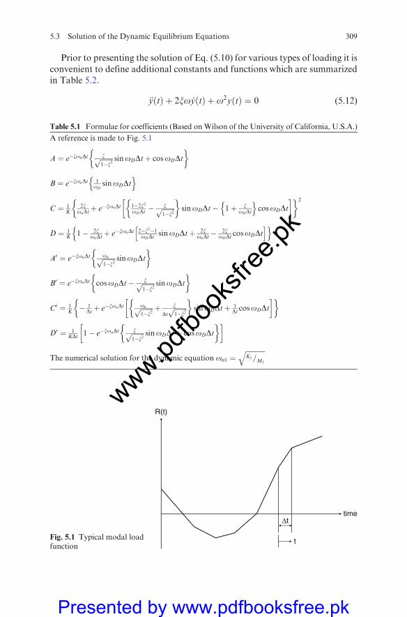
Prior to presenting the solution of Eq. (5.10) for various types of loading it isconvenient to define additional constants and functions which are summarizedin Table 5.2.
€yðtÞ þ 2xo _yðtÞ þ o2yðtÞ ¼ 0 (5:12)
Table 5.1 Formulae for coefficients (Based onWilson of the University of California, U.S.A.)
A reference is made to Fig. 5.1
A ¼ e�zonDt zffiffiffiffiffiffiffiffi1�x2p sinoDDtþ cosoDDt� �
B ¼ e�xonDt 1oD
sinoDDtn o
C ¼ 1K
2xonDtþ e�xonDt 1�2x2
oDDt� xffiffiffiffiffiffiffiffi
1�x2p
� �sinoDDt� 1þ x
oDDt
n ocosoDDt
� �� �2
D ¼ 1K 1� 2x
onDtþ e�xonDt 2�x2�1
oDDtsinoDDtþ 2x
onDt� 2x
oDDtcosoDDt
h in o
A0 ¼ e�xonDt onffiffiffiffiffiffiffiffi1�x2p sinoDDt� �
B0 ¼ e�xonDt cosoDDt� xffiffiffiffiffiffiffiffi1�x2p sinoDDt
� �
C0 ¼ 1K� 1
Dtþ e�xonDt onffiffiffiffiffiffiffiffi1�x2p þ x
Dtffiffiffiffiffiffiffiffi1�x2p
� �sinoDDtþ 1
Dt cosoDDt� �� �
D0 ¼ 1KDt 1� e�xonDt xffiffiffiffiffiffiffiffi
1�x2p sinoDDtþ cosoDDt� �� �
The numerical solution for the dynamic equation on1 ¼ffiffiffiffiffiffiffiffiffiffiffiffiK1=M1
q
R(t)
Δt
t
time
Fig. 5.1 Typical modal loadfunction
5.3 Solution of the Dynamic Equilibrium Equations 309
www.pdfbo
oksfr
ee.pk
Presented by www.pdfbooksfree.pk
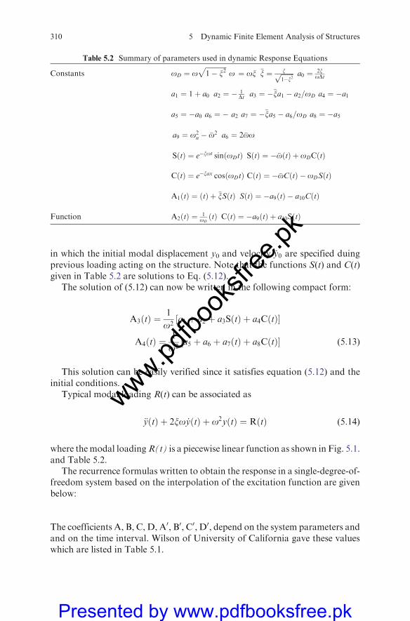
in which the initial modal displacement y0 and velocity _y0 are specified duingprevious loading acting on the structure. Note that the functions S(t) and C(t)given in Table 5.2 are solutions to Eq. (5.12).
The solution of (5.12) can now be written in the following compact form:
A3ðtÞ ¼1
o2½a1 þ a2 þ a3SðtÞ þ a4CðtÞ�
A4ðtÞ ¼1
o2½a5 þ a6 þ a7ðtÞ þ a8CðtÞ� (5:13)
This solution can be easily verified since it satisfies equation (5.12) and theinitial conditions.
Typical modal loading R(t) can be associated as
€yðtÞ þ 2xo _yðtÞ þ o2yðtÞ ¼ RðtÞ (5:14)
where the modal loadingR(t) is a piecewise linear function as shown in Fig. 5.1.and Table 5.2.
The recurrence formulas written to obtain the response in a single-degree-of-freedom system based on the interpolation of the excitation function are givenbelow:
The coefficients A, B, C, D, A0, B0, C0, D0, depend on the system parameters andand on the time interval. Wilson of University of California gave these valueswhich are listed in Table 5.1.
Table 5.2 Summary of parameters used in dynamic Response Equations
Constants oD ¼ offiffiffiffiffiffiffiffiffiffiffiffiffi1� x2
po ¼ ox �x ¼ xffiffiffiffiffiffiffiffi
1�x2p a0 ¼ 2x
oDt
a1 ¼ 1þ a0 a2 ¼ � 1Dt a3 ¼ ��xa1 � a2=oD a4 ¼ �a1
a5 ¼ �a0 a6 ¼ � a2 a7 ¼ ��xa5 � a6=oD a8 ¼ �a5
a9 ¼ o2n � �o2 a6 ¼ 2�oo
SðtÞ ¼ e�xot sinðoDtÞ SðtÞ ¼ ��oðtÞ þ oDCðtÞ
CðtÞ ¼ e�xax cosðoDtÞ CðtÞ ¼ ��oCðtÞ � oDSðtÞ
A1ðtÞ ¼ ðtÞ þ �xSðtÞ SðtÞ ¼ �a9ðtÞ � a10CðtÞ
Function A2ðtÞ ¼ 1oDðtÞ CðtÞ ¼ �a9ðtÞ þ a10SðtÞ
310 5 Dynamic Finite Element Analysis of Structures
www.pdfbo
oksfr
ee.pk
Presented by www.pdfbooksfree.pk
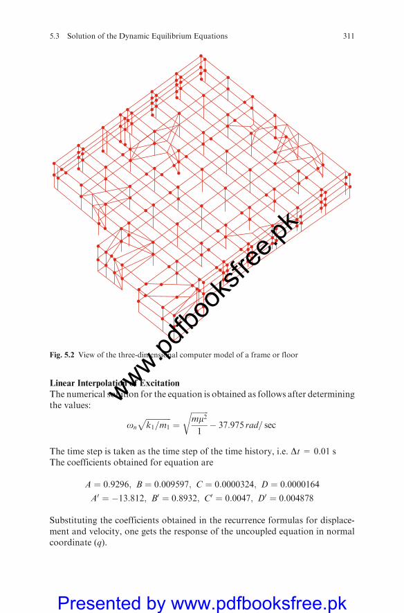
Linear Interpolation of Excitation
The numerical solution for the equation is obtained as follows after determiningthe values:
on
ffiffiffiffiffiffiffiffiffiffiffiffiffik1=m1
p¼
ffiffiffiffiffiffiffiffiffimm2
1
r� 37:975 rad= sec
The time step is taken as the time step of the time history, i.e. Dt = 0.01 sThe coefficients obtained for equation are
A ¼ 0:9296; B ¼ 0:009597; C ¼ 0:0000324; D ¼ 0:0000164
A0 ¼ �13:812; B0 ¼ 0:8932; C0 ¼ 0:0047; D0 ¼ 0:004878
Substituting the coefficients obtained in the recurrence formulas for displace-ment and velocity, one gets the response of the uncoupled equation in normalcoordinate (q).
Fig. 5.2 View of the three-dimensional computer model of a frame or floor
5.3 Solution of the Dynamic Equilibrium Equations 311
www.pdfbo
oksfr
ee.pk
Presented by www.pdfbooksfree.pk
5.4 Step-By-Step Solution Method
The most general solution method for dynamic analysis is an incremental
method in which the equilibrium equations are solved at times Dt, 2Dt, 3Dt,etc. There are a large number of different incremental solution methods
described in this chapter. In general, they involve a solution of the complete
set of equilibrium equations at each time increment. In the case of non-linear
analysis, it may be necessary to reform the stiffness matrix for the complete
structural system for each time step. Also, iterationmay be required within each
time increment to satisfy equilibrium. As a result of the large computational
requirements it can take a significant amount of time to solve structural systems
with just a few hundred degrees of freedom.In addition, artificial or numerical damping must be added to most incre-
mental solution methods in order to obtain stable solutions. For this reason,
engineers must be very careful in the interpretation of the results. For some non-
linear structures, subjected to seismic motions, incremental solution methods
are necessary.For very large structural systems, a combination of mode superposition and
incremental methods has been found to be efficient for systems with a small
number of non-linear members as stated byWilson of University of California.The response of real structures, when subjected to large dynamic loads, often
involves significant non-linear behaviour. In general, non-linear behaviour
includes the effects of large displacements and/or non-linear material
properties.The more complicated problem associated with large displacements, which
cause large strains in all members of the structures, requires a tremendous
amount of computational effort and computer time to obtain a solution. How-
ever, certain types of large strains, such as those in rubber base isolators and gap
elements, can be treated as a lumped non-linear element by the fast non-linear
analysis (FNA) method.
5.4.1 Fundamental Equilibrium Equations
The global dynamic equilibrium equations, at time t, of an elastic structure with
non-linear or energy-dissipating elements are of the following form:Looking at Eq. (5.2) it is now rewritten as
M €UðtÞ þ CinðtÞ þ KnðtÞ þ RðtÞn ¼ RðtÞ (5:15a)
All elements in the equation have already been defined. In addition R(t) is the
external applied load where RðtÞ ¼ FðtÞ ¼ SNj fjgðtÞj. R(t)N is the global mode
force vector due to the sum of the forces in the non-linear elements and is
312 5 Dynamic Finite Element Analysis of Structures
www.pdfbo
oksfr
ee.pk
Presented by www.pdfbooksfree.pk
computed by iteration at time t. The solution of structural systems with alimited number of non-linear elements is summarized below.
The first step in the solution of Eq. (5.12) is to calculate a set of ‘‘m’’orthogonal Ritz vectors, F , which satisfy the following equations of Eq. (5.7):
FT00M F ¼ 1 and (5:16a)
FT00K F ¼ O2 (5:16b)
where I is a unit matrix and O2 is a diagonal matrix in which the diagonal termsare defined.
The result is of great importance for the interpretation of the behaviour ofisolated buildings and for their preliminary design: and for the usual spectralshapes, the isolation system can be designed for a maximum displacement equalto , and the superstructure for a shear coefficient equal to . These values couldhave been obtained with reference to a simple oscillator, whose mass is equal tothe total mass of the superstructure and the stiffness and damping are equal tothe corresponding quantities of the isolation system.
The interstorey drift, on which the damage produced by an earthquakedepends, is proportional to the frequency ratio
ffiffiffiffiBp
and to the maximum basedisplacement.
5.4.2 Supplementary Devices
Supplementary devices are installed separately from isolators to complete theisolation system. Very often they are made of simple energy-dissipating ele-ments (EDEs). EDEs are sometimes embodied in isolators to improve theirenergy-dissipating capabilities and avoid the use of separate devices. They haveto be within the finite element systems equations.
5.4.2.1 Design Seismic Action Effects on Fixed-Base and Isolated Buildings
The stresses on fixed-base framed structure and on a similar isolated structureneed to be compared in terms of base shear on the superstructure. Therefore,the ratio between the design spectral accelerations of a fixed-base structuremultiplied by the effective mass ratio and that of a similar seismic-isolatedstructure divided by the behaviour factor of 1.5 for the superstructure iscalculated, where is the period of the fixed-base structure and the period ofthe isolated structure. The effective mass ratio is taken as equal to 0.85, asprescribed for the equivalent linear static analysis, if the structure has at leasttwo storeys and its vibration period is . It is taken equal to 1 for the isolatedstructure.
5.4 Step-By-Step Solution Method 313
www.pdfbo
oksfr
ee.pk
Presented by www.pdfbooksfree.pk
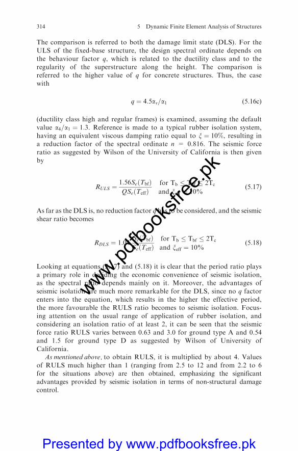
The comparison is referred to both the damage limit state (DLS). For the
ULS of the fixed-base structure, the design spectral ordinate depends onthe behaviour factor q, which is related to the ductility class and to the
regularity of the superstructure along the height. The comparison isreferred to the higher value of q for concrete structures. Thus, the case
with
q ¼ 4:5av=a1 (5:16c)
(ductility class high and regular frames) is examined, assuming the default
value a4=a1 ¼ 1:3. Reference is made to a typical rubber isolation system,having an equivalent viscous damping ratio equal to x ¼ 10%, resulting ina reduction factor of the spectral ordinate n = 0.816. The seismic force
ratio as suggested by Wilson of the University of California is then givenby
RULS ¼1:56SeðTbfÞQSeðTeffÞ
for Tb � Tbf � 2Tc
and xeff ¼ 10%(5:17)
As far as the DLS is, no reduction factor q has to be considered, and the seismic
shear ratio becomes
RDLS ¼ 1:04SeðTbfÞSeðTeffÞ
for Tb � Tbf � 2Tc
and xeff ¼ 10%(5:18)
Looking at equations (5.17) and (5.18) it is clear that the period ratio plays
a primary role in deciding the economic convenience of seismic isolation,as the spectral ratio depends mainly on it. Moreover, the advantages of
seismic isolation are much more remarkable for the DLS, since no q factorenters into the equation, which results in the higher the effective period,
the more favourable the RULS ratio becomes to seismic isolation. Focus-ing attention on the usual range of application of rubber isolation, andconsidering an isolation ratio of at least 2, it can be seen that the seismic
force ratio RULS varies between 0.63 and 3.0 for ground type A and 0.54and 1.5 for ground type D as suggested by Wilson of University of
California.As mentioned above, to obtain RULS, it is multiplied by about 4. Values
of RULS much higher than 1 (ranging from 2.5 to 12 and from 2.2 to 6for the situations above) are then obtained, emphasizing the significant
advantages provided by seismic isolation in terms of non-structural damagecontrol.
314 5 Dynamic Finite Element Analysis of Structures
www.pdfbo
oksfr
ee.pk
Presented by www.pdfbooksfree.pk
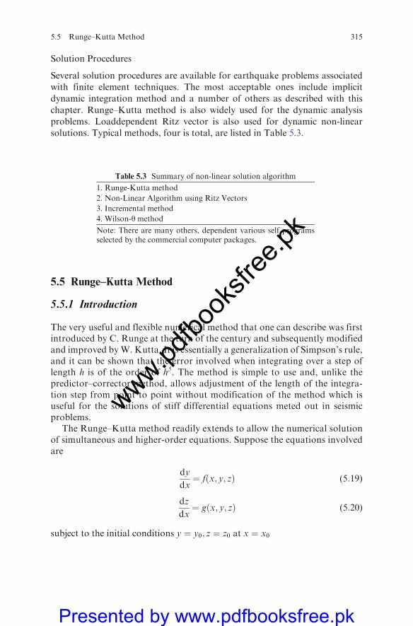
Solution Procedures
Several solution procedures are available for earthquake problems associated
with finite element techniques. The most acceptable ones include implicit
dynamic integration method and a number of others as described with this
chapter. Runge–Kutta method is also widely used for the dynamic analysis
problems. Loaddependent Ritz vector is also used for dynamic non-linear
solutions. Typical methods, four is total, are listed in Table 5.3.
5.5 Runge–Kutta Method
5.5.1 Introduction
The very useful and flexible numerical method that one can describe was firstintroduced by C. Runge at the turn of the century and subsequently modifiedand improved byW. Kutta. It is essentially a generalization of Simpson’s rule,and it can be shown that the error involved when integrating over a step oflength h is of the order of h5. The method is simple to use and, unlike thepredictor–corrector method, allows adjustment of the length of the integra-tion step from point to point without modification of the method which isuseful for the solutions of stiff differential equations meted out in seismicproblems.
The Runge–Kutta method readily extends to allow the numerical solutionof simultaneous and higher-order equations. Suppose the equations involvedare
dy
dx¼ fðx; y; zÞ (5:19)
dz
dx¼ gðx; y; zÞ (5:20)
subject to the initial conditions y ¼ y0; z ¼ z0 at x ¼ x0
Table 5.3 Summary of non-linear solution algorithm
1. Runge-Kutta method
2. Non-Linear Algorithm using Ritz Vectors
3. Incremental method
4. Wilson-y method
Note: There are many others, dependent various self programsselected by the commercial computer packages.
5.5 Runge–Kutta Method 315
www.pdfbo
oksfr
ee.pk
Presented by www.pdfbooksfree.pk
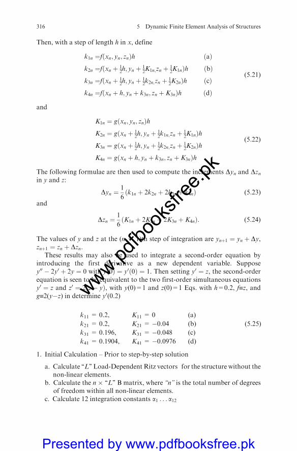
Then, with a step of length h in x, define
k1n ¼fðxn; yn; znÞh ðaÞ
k2n ¼fðxn þ 12h; yn þ 1
2K1n;zn þ 12K1nÞh ðbÞ
k3n ¼fðxn þ 12h; yn þ 1
2k2n;zn þ 12K2nÞh ðcÞ
k4n ¼fðxn þ h; yn þ k3n; zn þ K3nÞh ðdÞ
(5:21)
and
K1n ¼ gðxn; yn; znÞh
K2n ¼ gðxn þ 12h; yn þ 1
2k1n;zn þ 12K1nÞh
K3n ¼ gðxn þ 12h; yn þ 1
2k2n;zn þ 12K2nÞh
K4n ¼ gðxn þ h; yn þ k3n; zn þ K3nÞh
(5:22)
The following formulae are then used to compute the increments Dyn and Dznin y and z:
Dyn ¼1
6k1n þ 2k2n þ 2k3n þ k4nð Þ (5:23)
and
Dzn ¼1
6K1n þ 2K2n þ 2K3n þ K4nð Þ: (5:24)
The values of y and z at the (n + 1)th step of integration are ynþ1 ¼ yn þ Dy,znþ1 ¼ zn þ Dzn:
These results may also be used to integrate a second-order equation byintroducing the first derivative as a new dependent variable. Supposey00 � 2y0 þ 2y ¼ 0 with y 0ð Þ ¼ y0 0ð Þ ¼ 1. Then setting y0 ¼ z, the second-orderequation is seen to be equivalent to the two first-order simultaneous equationsy0 ¼ z and z0 ¼ 2 z� yð Þ, with y(0)=1 and z(0)=1 Eqs. with h=0.2, f”z, andg”2(y�z) in determine y0(0.2)
1. Initial Calculation – Prior to step-by-step solution
a. Calculate ‘‘L’’ Load-Dependent Ritz vectors for the structure without thenon-linear elements.
b. Calculate the n � ‘‘L’’ B matrix, where ‘‘n’’ is the total number of degreesof freedom within all non-linear elements.
c. Calculate 12 integration constants a1 . . . a12
k11 = 0.2, K11 = 0 (a)
k21 = 0.2, K21 = �0.04 (b) (5.25)
k31 = 0.196, K31 = �0.048 (c)
k41 = 0.1904, K41 = �0.0976 (d)
316 5 Dynamic Finite Element Analysis of Structures
www.pdfbo
oksfr
ee.pk
Presented by www.pdfbooksfree.pk
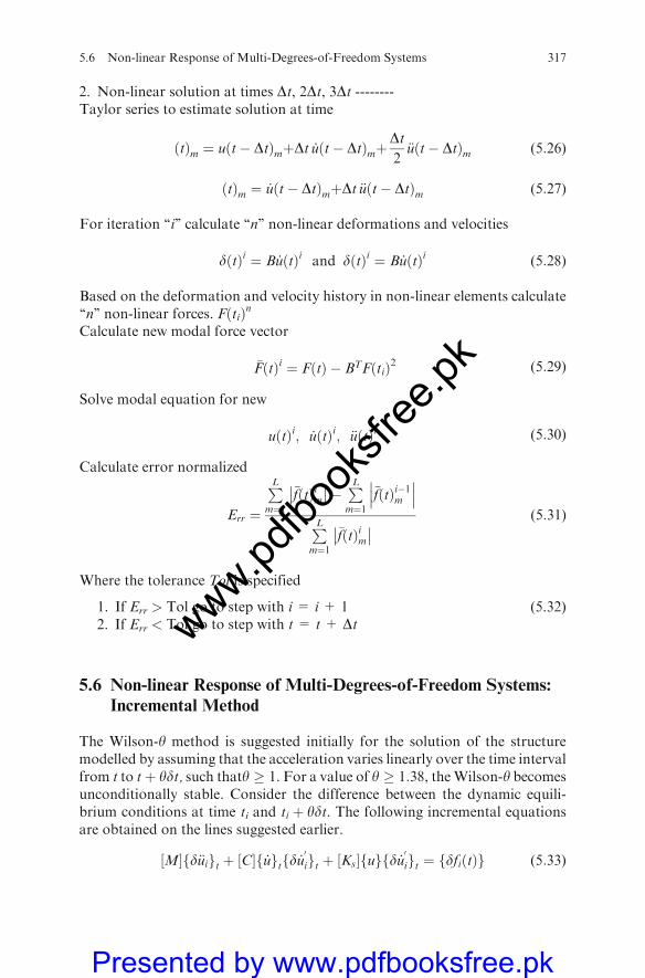
2. Non-linear solution at times Dt, 2Dt, 3Dt --------Taylor series to estimate solution at time
ðtÞm ¼ u t� Dtð ÞmþDt _u t� Dtð ÞmþDt2
€u t� Dtð Þm (5:26)
ðtÞm ¼ _u t� Dtð ÞmþDt €u t� Dtð Þm (5:27)
For iteration ‘‘i’’ calculate ‘‘n’’ non-linear deformations and velocities
dðtÞi ¼ B _uðtÞi and dðtÞi ¼ B _uðtÞi (5:28)
Based on the deformation and velocity history in non-linear elements calculate‘‘n’’ non-linear forces. F tið ÞnCalculate new modal force vector
�FðtÞi ¼ FðtÞ � BTF tið Þ2 (5:29)
Solve modal equation for new
uðtÞi; _uðtÞi; €uðtÞi (5:30)
Calculate error normalized
Err ¼
PLm¼1
�fðtÞim�� ��� PL
m¼1�fðtÞi�1m
��� ���PLm¼1
�fðtÞim�� �� (5:31)
Where the tolerance Tol is specified
1. If Err > Tol go to step with i = i + 1 (5.32)2. If Err < Tol go to step with t = t + Dt
5.6 Non-linear Response of Multi-Degrees-of-Freedom Systems:
Incremental Method
The Wilson-y method is suggested initially for the solution of the structuremodelled by assuming that the acceleration varies linearly over the time intervalfrom t to tþ ydt, such thaty � 1. For a value of y � 1:38, theWilson-y becomesunconditionally stable. Consider the difference between the dynamic equili-brium conditions at time ti and ti þ ydt. The following incremental equationsare obtained on the lines suggested earlier.
½M�fd€uigt þ ½C�f _ugtfd _u0
igt þ ½Ks�fugfd _u0
igt ¼ fdfiðtÞg (5:33)
5.6 Non-linear Response of Multi-Degrees-of-Freedom Systems 317
www.pdfbo
oksfr
ee.pk
Presented by www.pdfbooksfree.pk
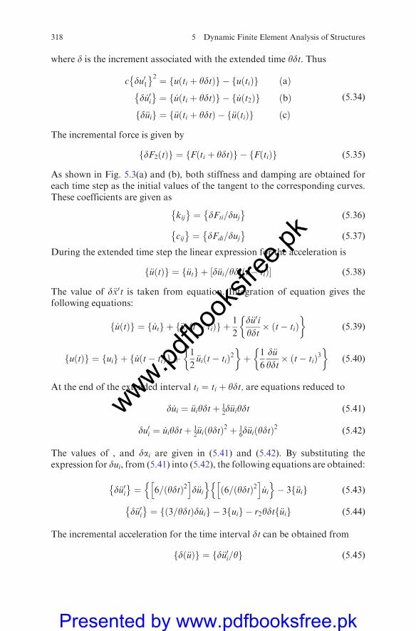
where d is the increment associated with the extended time ydt. Thus
c du01� 2 ¼ u ti þ ydtð Þf g � u tið Þf g að Þ
d _u0i�
¼ _u ti þ ydtð Þf g � _u t2ð Þf g bð Þ
d€uif g ¼ f€uðti þ ydtÞ � f€uðtiÞg cð Þ
(5:34)
The incremental force is given by
dF2ðtÞf g ¼ F ti þ ydtð Þf g � F tið Þf g (5:35)
As shown in Fig. 5.3(a) and (b), both stiffness and damping are obtained foreach time step as the initial values of the tangent to the corresponding curves.These coefficients are given as
kij�
¼ dFti=duj�
(5:36)
cij�
¼ dFdi=duj�
(5:37)
During the extended time step the linear expression for the acceleration is
€uðtÞf g ¼ €utf g þ d€ui=ydt t� tið Þ½ � (5:38)
The value of d€x0t is taken from equation. Integration of equation gives thefollowing equations:
_uðtÞf g ¼ _utf g þ €a1 t� tið Þf g þ 1
2
d€u0i
ydt� t� tið Þ
� �(5:39)
uðtÞf g ¼ uif g þ _u t� tið Þf g þ 1
2€ui t� tið Þ2
� �þ 1
6
d€u
ydt� t� tið Þ3
� �(5:40)
At the end of the extended interval ti ¼ ti þ ydt, are equations reduced to
d _ui ¼ €uiydtþ 12d€uiydt (5:41)
du0i ¼ _uiydtþ 12€uiðydtÞ2 þ 1
6d€uiðydtÞ2 (5:42)
The values of , and dai are given in (5.41) and (5.42). By substituting theexpression for dui, from (5.41) into (5.42), the following equations are obtained:
d€u0i�
¼ 6=ðydtÞ2h i
d€ui
n oð6=ðydtÞ2h i
_ui
n o� 3 €uif g (5:43)
d€u0i�
¼ ð3=ydtÞd _uif g � 3fuig � r2ydtf€uig (5:44)
The incremental acceleration for the time interval dt can be obtained from
dð€uÞf g ¼ fd€u0i=yg (5:45)
318 5 Dynamic Finite Element Analysis of Structures
www.pdfbo
oksfr
ee.pk
Presented by www.pdfbooksfree.pk
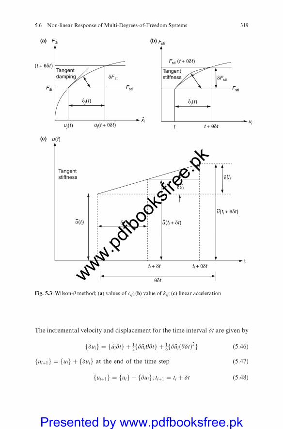
The incremental velocity and displacement for the time interval dt are given by
duif g ¼ f _uidtg þ 12fd€uiydtg þ 1
6fd€uiðydtÞ2g (5:46)
fuiþ1g ¼ fuig þ fduig at the end of the time step (5:47)
fuiþ1g ¼ fuig þ fduig; tiþ1 ¼ ti þ dt (5:48)
(t + θδt )
δj(t )
uj(t + θδt )uj(t )
Fdi
Fdi Fsti
δFsti
Tangentdamping
(a)
(c)
(b)
Fsti (t + θδt )
δj(t )
t + θδtt
Fsti
Fsti
δFsti
Tangentstiffness
δu i
u (ti)
u (ti + θδt )
t
u (t )
δu i
δt
Tangentstiffness
ti + θδt
u (ti + δt)••••
••
••
ti + δt
θδt
xi•
ui
••
Fig. 5.3 Wilson-y method; (a) values of cij; (b) value of kij; (c) linear acceleration
5.6 Non-linear Response of Multi-Degrees-of-Freedom Systems 319
www.pdfbo
oksfr
ee.pk
Presented by www.pdfbooksfree.pk
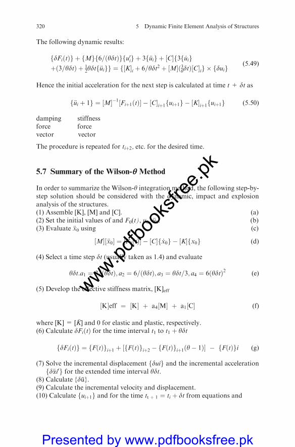
The following dynamic results:
fdFiðtÞg þ fMgf6=ðydtÞgfu0ig þ 3f€uig þ ½C�f3f _uigþð3=ydtÞ þ 1
2ydtf€uigg ¼ f½K�i þ 6=ydt2 þ ½M�ð3ydtÞ½C�ig � fduig(5:49)
Hence the initial acceleration for the next step is calculated at time t + dt as
€ui þ 1f g ¼ M½ ��1 Fiþ1ðtÞ½ � � C½ �iþ1 uiþ1f g � K½ �iþ1 uiþ1f g (5:50)
damping stiffnessforce forcevector vector
The procedure is repeated for tiþ2, etc. for the desired time.
5.7 Summary of the Wilson-q Method
In order to summarize the Wilson-y integration method, the following step-by-step solution should be considered with the dynamic, impact and explosionanalysis of the structures.(1) Assemble [K], [M] and [C]. (a)(2) Set the initial values of and F0(t), u0, €u0. (b)(3) Evaluate €x0 using (c)
M½ � €x0½ � ¼ F0ðtÞ½ � � C½ � _x0f g � K½ � x0f g (d)
(4) Select a time step dt (usually taken as 1.4) and evaluate
ydt:a1 ¼ 3= ydtð Þ; a2 ¼ 6= ydtð Þ; a3 ¼ ydt=3; a4 ¼ 6 ydtð Þ2 (e)
(5) Develop the effective stiffness matrix, [K]eff
½K�eff ¼ ½K� þ a4½M� þ a1½C� (f)
where [K] = [ �K] and 0 for elastic and plastic, respectively.(6) Calculate dFiðtÞ for the time interval t1 to t1 þ ydt
fdFiðtÞg ¼ fFðtÞgiþ1 þ ½fFðtÞgiþ2 � fFðtÞgiþ1ðy� 1Þ� � fFðtÞgi (g)
(7) Solve the incremental displacement duif g and the incremental accelerationd€ai0f g for the extended time interval ydt.
(8) Calculate {du}.(9) Calculate the incremental velocity and displacement.(10) Calculate fuiþ1g and for the time tt þ 1 ¼ ti þ dt from equations and
320 5 Dynamic Finite Element Analysis of Structures
www.pdfbo
oksfr
ee.pk
Presented by www.pdfbooksfree.pk
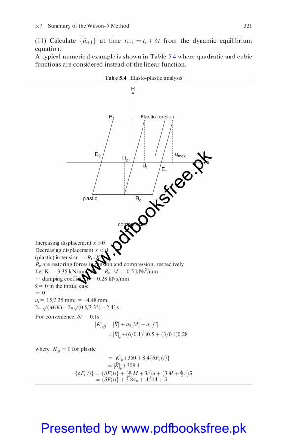
(11) Calculate f€uiþ1g at time tt�1 ¼ ti þ dt from the dynamic equilibrium
equation.A typical numerical example is shown in Table 5.4 where quadratic and cubic
functions are considered instead of the linear function.
Table 5.4 Elasto-plastic analysis
xE1
R
Rc
Rt
Ut
E2 umaxUc
compression
plastic
Plastic tension
Increasing displacement x >0
Decreasing displacement x < 0
(plastic) in tension = Rt /K
Re are restoring forces in tension and compression, respectively
Let K = 3.35 kN/mm; Rt = Re; M = 0.5 kNs2/mm
= damping coefficient = 0.28 kNs/mm
_x= 0 in the initial case
= 0
ut= 15/3.35 mm; = –4.48 mm;
2pp(M/K)=2p
p(0.5/3.35)=2.43 s
For convenience, dt = 0.1s
K½ �eff ¼ �K½ � þ a4 M½ � þ a1 C½ �¼ �K½ �pþ 6=0:1ð Þ2Þ0:5þ 3=0:1ð Þ0:28
where ½K�p ¼ 0 for plastic
¼ �K½ �pþ350þ 8:4 dF2ðtÞf g¼ �K½ �pþ308:4
dFiðtÞf g ¼ dFðtÞf g þ 6dtMþ 3c �
_uþ 3Mþ dt2 c
�€u
¼ dFðtÞf g þ 3:84u þ :1514þ €u
5.7 Summary of the Wilson-y Method 321
www.pdfbo
oksfr
ee.pk
Presented by www.pdfbooksfree.pk
5.8 Dynamic Finite Element Formulation with Base Isolation
Seismic response of the base-isolated buildings, excited unidirectionally
with these ground motions can be obtained by means of computer program
ISOPAR-II. This program is given a detailed review in the Appendix.The following assumptions are made in this software for the analysis of base-
isolated buildings:
(i) The superstructure is elastic at all times and the non-linear behaviour isrestricted in isolators only.
(ii) All framed substructures are connected at each floor level by a diaphragm,which is infinitely rigid in its own plane.
(iii) Each floor has three degrees of freedom (two translations and one rotation)attached to the centre of mass of each floor.
(iv) The isolation devices are rigid in the vertical direction and have negligibletorsion resistance.
The equations of motion for the elastic superstructure are expressed in the
following form familiar from the dynamic equations stated earlier inclusive of
ground acceleration.
Mu þ Cu þ Ku ¼ �MR €ug þ €ub�
(5:51)
where
M = mass matrix for superstructureC = damping matrix for superstructureK = stiffness matrix for superstructureR = the matrix of influence coefficientu = the vector of floor displacement relative to baseub = the vector of base displacement relative to ground andug = the vector of ground acceleration
The velocity increment is given by
d _u ¼ 3=dtð Þdui � 3 _ui � dt=2ð Þ€ui
¼ 3=0:1ð Þdui � 3 _ui 0:12ð Þ€u1¼30dui � 3 _ui � 0:05€ui
The results are obtained on the basis of the above two equations of force and velocityincrement. The step-by-step procedure is covered in Section 3.4.6 and the results are tabulatedas follows.
t FðtÞ x _x R €x �Kp
� Keff½ � dFðtÞ d �FðtÞ dx d _x
Table 5.4 (continued)
322 5 Dynamic Finite Element Analysis of Structures
www.pdfbo
oksfr
ee.pk
Presented by www.pdfbooksfree.pk
The equations of motion for the base are
RTM½f€ug þ Rf€ub þ €ugg� þ ½Mb�f€ub þ €uggþ½Cb�fubg þ ½ _kb�fubg þ ffg ¼ 0
(5:52)
where
Mb = mass matrix for base isolation systemCb = damping matrix for base isolation systemKb = stiffness matrix for base isolation system andf = the vector containing the forces mobilized in the non-linear elements
of the isolation system
Employing modal reduction
u ¼ fu (5:53)
where
f= the modal matrix normalized with respect to the mass matrix andu = the modal displacement vector relative to the base and combining
equations the following equation is obtained:
½I� fT 00mR
RT 00mf RT 00mRþ _Mb
" #€u
€ub
� �þ
2zioi 0
0 Cb
� �€u
_ub
� �
þ o2i 0
0 Rb
� �_u
ub
� �þ
0
f
� �¼ � fT 00mR
RT 00mRþmb
" #€ug � (5:54)
5.9 Added Viscoelastic Dampers (VEDs) in Seismic Buildings
5.9.1 Introduction
The effect of supporting braces on the controlled efficiency ofVEDs is investigated.It is, on the basis if available evidence, considered that when sufficient stiffnesscannot be provided for the supporting braces, if required, the flexibility of the braceshould be considered in the design of the VED to achieve the desired performanceof the building. Sometimes it is necessary, if compensation is needed, to reduce thesize of the supporting brace to increase the additional VED size.
The viscoelastic damper (VED) is acknowledged as one of the most efficientenergy-absorbing devices for building structures against dynamic loads such asearthquake or wind. Previous studies have shown that the efficiency of an addedVED can be greatly enhanced by applying properly sized dampers to properlocations. Zhang and Soong and Shukla and Datta have proposed optimallocation and size of the VED.
5.9 Added Viscoelastic Dampers (VEDs) in Seismic Buildings 323
www.pdfbo
oksfr
ee.pk
Presented by www.pdfbooksfree.pk
5.9.2 Generalized Equation of Motion when Dampers Are Used
Equations (5.1), (5.42) and (5.44) are modified to include the influence of thedamper under consideration. The equation of motion of an n-degree-of-free-dom building structure with supplementary dampers installed at different loca-tions and subjected to ground excitations at the base can be written as
ms€usðtÞ þ cs _uðtÞ þ ksusðtÞ þXme
d¼1�r di p drðtÞ ¼ �msegi€ugðtÞ (5:55)
wherems, ks and cs, respectively, represent the n� nmass, stiffness, and inherentstructural damping matrices of the building structure. €ugðtÞ = ground accel-eration time history; e = ground motion influence coefficients; and usðtÞ= n-dimensional relative displacement response vector measured with respect to thebase.
A dot over a quantity indicates time derivative of the quantity. pdrðtÞ repre-sents the force in the damper at the dth location, and there are N number ofpossible locations where the devices can be installed on the structure. Theinfluence of the damper force on the structure is considered through the n-dimensional influence vector. It is assumed that the structural system behaveslinearly under earthquake-induced ground excitation.
5.9.3 System Dynamic Equation with Friction Dampers
The governing equation of motion given earlier in this chapter such as Eq. (5.1)can now be slightly modified for the whole system (superstructure of thebuilding, sliding support and semi-active/passive dampers) and can be statedas without dampers (semi-active or passive) but sliding included of the buildingsupport
m½ � €uf g þ c½ � _uf g þ Pd uð Þf g ¼ � m½ � I½ � €ug�
(5:56)
in which
[m]=mass matrix; [c] damping matrix{u}= linear case[k] = elastic stiffness matrix
{u}T0 0= displacement vector
I = identity matrix or unit diagonal matrix
The differential equations of motion (5.49) are solved in incremental form byemploying the Newmark–Beta method assuming a constant average accelera-tion over a short time interval. In convergent process the Newton–Raphsonmethod is used for the solution of the non-linear problem and the iteration
324 5 Dynamic Finite Element Analysis of Structures
www.pdfbo
oksfr
ee.pk
Presented by www.pdfbooksfree.pk
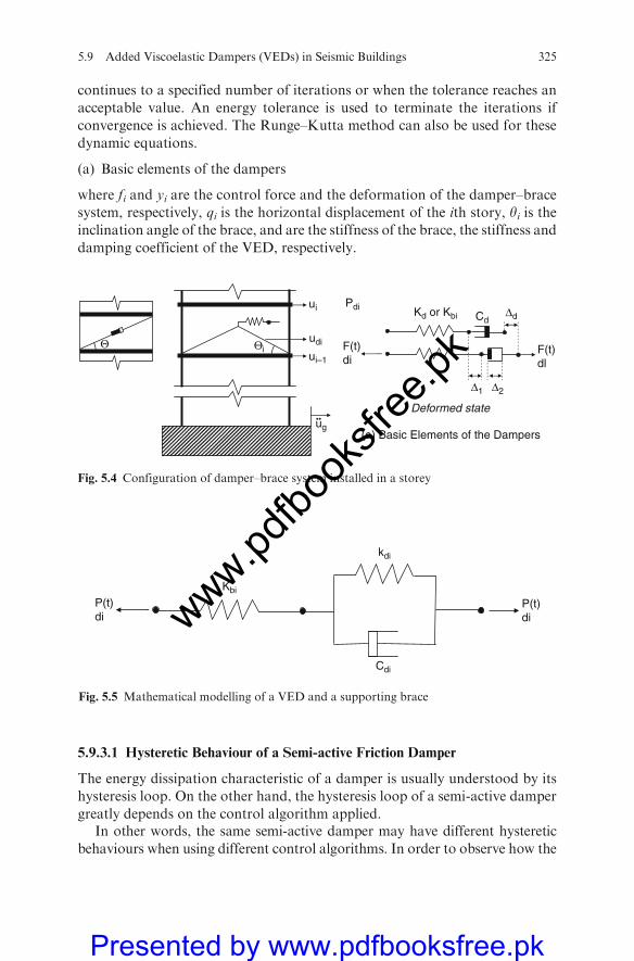
continues to a specified number of iterations or when the tolerance reaches an
acceptable value. An energy tolerance is used to terminate the iterations if
convergence is achieved. The Runge–Kutta method can also be used for these
dynamic equations.
(a) Basic elements of the dampers
where fi and yi are the control force and the deformation of the damper–brace
system, respectively, qi is the horizontal displacement of the ith story, yi is theinclination angle of the brace, and are the stiffness of the brace, the stiffness and
damping coefficient of the VED, respectively.
5.9.3.1 Hysteretic Behaviour of a Semi-active Friction Damper
The energy dissipation characteristic of a damper is usually understood by its
hysteresis loop. On the other hand, the hysteresis loop of a semi-active damper
greatly depends on the control algorithm applied.In other words, the same semi-active damper may have different hysteretic
behaviours when using different control algorithms. In order to observe how the
Deformed state
Θ Θi
(a) Basic Elements of the Dampers
udi
ui
Δ1 Δ2
CdΔdKd or Kbi
F(t)dl
F(t)di
Pdi
ui–1
ug••
Fig. 5.4 Configuration of damper–brace system installed in a storey
Cdi
Kbi
kdi
P(t)di
P(t)di
Fig. 5.5 Mathematical modelling of a VED and a supporting brace
5.9 Added Viscoelastic Dampers (VEDs) in Seismic Buildings 325
www.pdfbo
oksfr
ee.pk
Presented by www.pdfbooksfree.pk
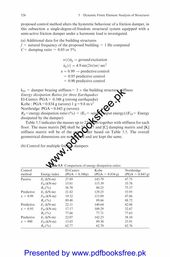
proposed control method alters the hysteretic behaviour of a friction damper, in
this subsection a single-degree-of-freedom structural system equipped with a
semi-active friction damper under a harmonic load is investigated.
(a) Additional data for the building structuresf = natural frequency of the proposed building = 1 Hz computedC= damping ratio = 0.05 or 5%
wðtÞ€ug ¼ ground excitation
€ugðtÞ ¼ 4:9 sin 2ptð Þm= sec2
a ¼ 0:99! predictive control
= 0.95 predictive control= 0.90 predictive control
kD = damper bracing stiffness= 3 � the building structure stiffnessEnergy dissipation Ratios for three EarthquakesEl-Centro: PGA= 0.348 g (strong earthquake)Kobe : PGA=0.834 g (severe) 1 g=9.8 m/s2
Northridge: PGA=0.843 g (severe)Rd=energy dissipation ratio (%) = (E1= seismic input energy)/(FD= Energy
dissipated by the damper)Table 5.5 indicates the masses up to 27 floors together with stiffness for each
floor. The mass matrix [M] shall be 27 � 27 and [C] damping matrix and [K]
stiffness matrix will be of the same order based on Table 5.5. The overall
geometrical dimensions are not altered and are kept the same.
(b) Control for multiple friction dampers
Table 5.5 Comparison of energy dissipation ratios
Controlmethod Energy index
El-Centro(PGA= 0.348g)
Kobe(PGA = 0.834 g)
Northridge(PGA = 0.843 g)
Passive E1 (kN-m) 27.89 143.79 47.75
FD (kN-m) 15.81 115.39 35.76
Rd (%) 56.70 80.25 75.37
Predictive E1 (kN-m) 21.82 129.25 53.95
a = 0.99 FD (kN-m) 19.52 115.89 47.86
Rd (%) 89.48 89.66 88.72
Predictive E1 (kN-m) 22.11 140.64 42.08
a = 0.95 FD (kN-m) 17.17 109.29 32.67
Rd (%) 77.66 77.71 77.63
Predictive E1 (kN-m) 22.07 142.23 38.10
a = 090 FD (kN-m) 13.85 89.30 23.91
Rd (%) 62.77 62.70 62.76
326 5 Dynamic Finite Element Analysis of Structures
www.pdfbo
oksfr
ee.pk
Presented by www.pdfbooksfree.pk
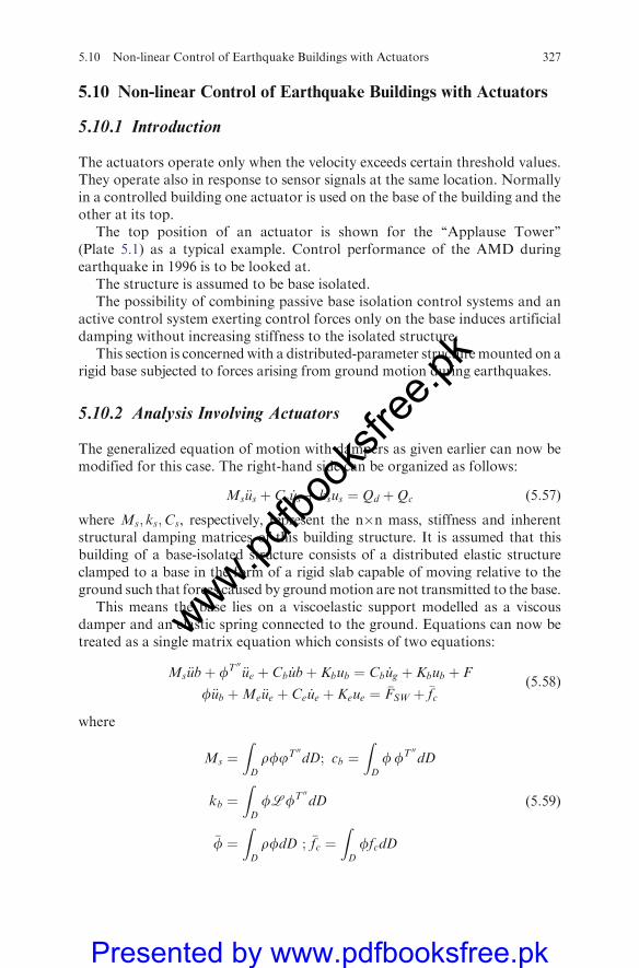
5.10 Non-linear Control of Earthquake Buildings with Actuators
5.10.1 Introduction
The actuators operate only when the velocity exceeds certain threshold values.They operate also in response to sensor signals at the same location. Normallyin a controlled building one actuator is used on the base of the building and theother at its top.
The top position of an actuator is shown for the ‘‘Applause Tower’’(Plate 5.1) as a typical example. Control performance of the AMD duringearthquake in 1996 is to be looked at.
The structure is assumed to be base isolated.The possibility of combining passive base isolation control systems and an
active control system exerting control forces only on the base induces artificialdamping without increasing stiffness to the isolated structure.
This section is concernedwith a distributed-parameter structuremounted on arigid base subjected to forces arising from ground motion during earthquakes.
5.10.2 Analysis Involving Actuators
The generalized equation of motion with dampers as given earlier can now bemodified for this case. The right-hand side can be organized as follows:
Ms€us þ Cs _us þ ksus ¼ Qd þQc (5:57)
where Ms; ks;Cs, respectively, represent the n�n mass, stiffness and inherentstructural damping matrices of this building structure. It is assumed that thisbuilding of a base-isolated structure consists of a distributed elastic structureclamped to a base in the form of a rigid slab capable of moving relative to theground such that forces caused by groundmotion are not transmitted to the base.
This means the base lies on a viscoelastic support modelled as a viscousdamper and an elastic spring connected to the ground. Equations can now betreated as a single matrix equation which consists of two equations:
Ms€ubþ fT 00 €ue þ Cb _ubþ Kbub ¼ Cb _ug þ Kbub þ F
f€ub þMe€ue þ Ce _ue þ Keue ¼ �FSW þ �fc(5:58)
where
Ms ¼ZD
rfjT 00dD; cb ¼ZD
ffT 00dD
kb ¼ZD
flfT 00dD
�f ¼ZD
rfdD ; �fc ¼ZD
ffcdD
(5:59)
5.10 Non-linear Control of Earthquake Buildings with Actuators 327
www.pdfbo
oksfr
ee.pk
Presented by www.pdfbooksfree.pk
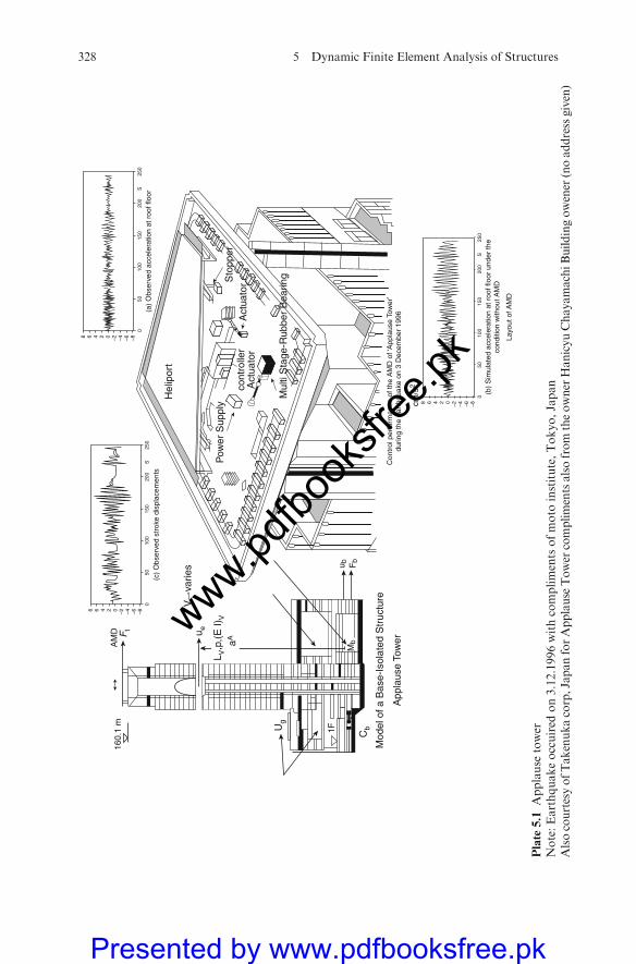
Pow
er S
uppl
y
Mod
el o
f a B
ase-
Isol
ated
Str
uctu
re
App
laus
e To
wer
Con
trol
per
form
ance
of t
he A
MD
of ‘
App
laus
e To
wer
’du
ring
the
eart
hqua
ke o
n 3
Dec
embe
r 19
96
(b)
Sim
ulat
ed a
ccel
erat
ion
at r
oof f
loor
und
er th
eco
nditi
on w
ithou
t AM
D
(a)
Obs
erve
d ac
cele
ratio
n at
roo
f flo
or(c
) O
bser
ved
stro
ke d
ispl
acem
ents
cm/s
2
CbU
g
Hel
ipor
t
cont
rolle
rA
ctua
tor
Act
uato
rSto
pper
Mul
ti S
tage
-Rub
ber
Bea
ring
Mb
1F
Fb
u b
8 6 4 2 –2 –4 –6 –80
5010
015
020
025
0S
0
8 6 4 2 –2 –4 –6 –80
5010
015
020
025
0S
0
8 6 4 2 –2 –4 –6 –80
5010
015
020
025
0S
0
160.
1 m
AM
D
L V,p
,(E
I)V
u eFt
V
varie
s
aA
Layo
ut o
f AM
D
Plate
5.1
Applause
tower
Note:Earthquakeoccuired
on3.12.1996withcomplimentsofmoto
institute,Tokyo,Japan
AlsocourtesyofTakenukacorp,JapanforApplause
Tower
complimentsalsofrom
theowner
HanicyuChayamachiB
uildingowener
(noaddressgiven)
328 5 Dynamic Finite Element Analysis of Structures
www.pdfbo
oksfr
ee.pk
Presented by www.pdfbooksfree.pk
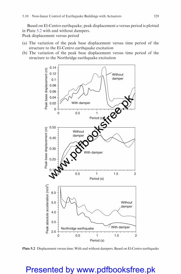
Based on El-Centro earthquake, peak displacement u versus period is plotted
in Plate 5.2 with and without dampers.Peak displacement versus period
(a) The variation of the peak base displacement versus time period of thestructure to the El-Centro earthquake excitation
(b) The variation of the peak base displacement versus time period of thestructure to the Northridge earthquake excitation
00
0.02
Pea
k ba
se d
ispl
acem
ent (
m)
0.04
0.06
0.08
0.1
0.12
0.14
0.5 1 1.5
Period (s)
With damper
Withoutdamper
0.15
Pea
k ba
se d
ispl
acem
ent (
m)
0.25
0.35
0.45
0.55
0 0.5 1 1.5 2
Period (s)
With damper
Withoutdamper
Pea
k ab
solu
te a
ccel
erat
ion
(m/s
2 )
2.5
3.5
4.5
5.5
6.5
0 0.5
Northridge earthquake
1 1.5 2
Period (s)
With damper
Withoutdamper
Plate 5.2 Displacement versus time;With andwithout dampers; Based on El-Centro earthquake
5.10 Non-linear Control of Earthquake Buildings with Actuators 329
www.pdfbo
oksfr
ee.pk
Presented by www.pdfbooksfree.pk
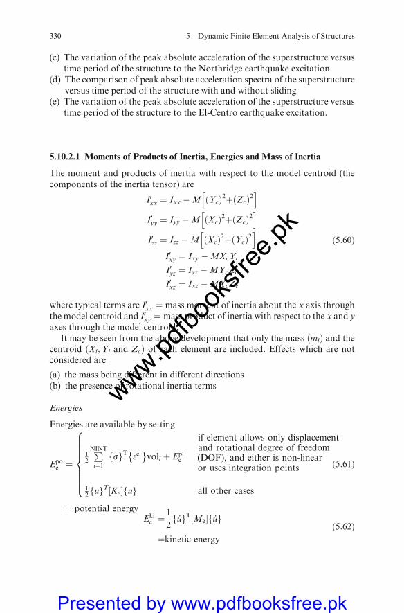
(c) The variation of the peak absolute acceleration of the superstructure versustime period of the structure to the Northridge earthquake excitation
(d) The comparison of peak absolute acceleration spectra of the superstructureversus time period of the structure with and without sliding
(e) The variation of the peak absolute acceleration of the superstructure versustime period of the structure to the El-Centro earthquake excitation.
5.10.2.1 Moments of Products of Inertia, Energies and Mass of Inertia
The moment and products of inertia with respect to the model centroid (thecomponents of the inertia tensor) are
I0xx ¼ Ixx �M Ycð Þ2þ Zcð Þ2h i
I0yy ¼ Iyy �M Xcð Þ2þ Zcð Þ2h i
I0zz ¼ Izz �M Xcð Þ2þ Ycð Þ2h i
I0xy ¼ Ixy �MXcYc
I0yz ¼ Iyz �MYcZc
I0xz ¼ Ixz �MXcZc
(5:60)
where typical terms are I0xx ¼ mass moment of inertia about the x axis throughthe model centroid and I0xy ¼ mass product of inertia with respect to the x and yaxes through the model centroid.
It may be seen from the above development that only the mass mið Þ and thecentroid Xi;Yi and Zcð Þ of each element are included. Effects which are notconsidered are
(a) the mass being different in different directions(b) the presence of rotational inertia terms
Energies
Energies are available by setting
Epoe ¼
12
PNINT
i¼1sf gT eel
� voli þ Epl
e
12
uf gT Ke½ � uf g
8>>>>>><>>>>>>:
if element allows only displacementand rotational degree of freedom(DOF), and either is non-linearor uses integration points
all other cases
(5:61)
¼ potential energyEkie ¼
1
2_uf gT Me½ � _uf g
¼kinetic energy
(5:62)
330 5 Dynamic Finite Element Analysis of Structures
www.pdfbo
oksfr
ee.pk
Presented by www.pdfbooksfree.pk
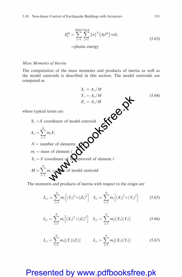
Eple ¼
XNINT
i¼1
XNCS
j¼1sf gT Depl
� voli
¼plastic energy
(5:63)
Mass Moments of Inertia
The computation of the mass moments and products of inertia as well asthe model centroids is described in this section. The model centroids arecomputed as
Xc ¼ Ax M=
Yc ¼ Ay=M
Zc ¼ Az=M
(5:64)
where typical terms are
Xc ¼X coordinate of model centroid
Ax ¼XNi¼1
miXi
N ¼ number of elements
mi ¼ mass of element i
Xi ¼X coordinate of the centroid of element i
M ¼XNi¼1
mi ¼ mass of model centroid
The moments and products of inertia with respect to the origin are
Ixx ¼XNi¼1
mi Yið Þ2þ Zið Þ2h i
Izz ¼XNi¼1
mi Xið Þ2þ Yið Þ2h i
(5:65)
Iyy ¼XNi¼1
mi Xið Þ2þ Zið Þ2h i
Ixy ¼XNi¼1
mi Xið Þ Yið Þ½ � (5:66)
Iyz ¼XNi¼1
mi Yið Þ Zið Þ½ � Ixz ¼XNi¼1
mi Xið Þ Yið Þ½ � (5:67)
5.10 Non-linear Control of Earthquake Buildings with Actuators 331
www.pdfbo
oksfr
ee.pk
Presented by www.pdfbooksfree.pk
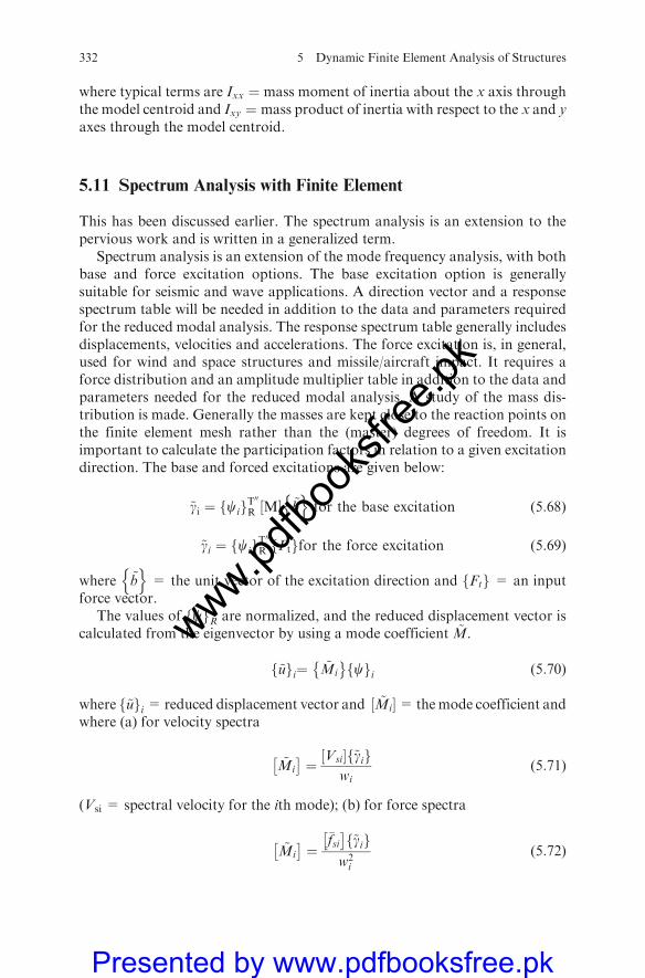
where typical terms are Ixx ¼ mass moment of inertia about the x axis throughthe model centroid and Ixy ¼ mass product of inertia with respect to the x and yaxes through the model centroid.
5.11 Spectrum Analysis with Finite Element
This has been discussed earlier. The spectrum analysis is an extension to thepervious work and is written in a generalized term.
Spectrum analysis is an extension of the mode frequency analysis, with bothbase and force excitation options. The base excitation option is generallysuitable for seismic and wave applications. A direction vector and a responsespectrum table will be needed in addition to the data and parameters requiredfor the reduced modal analysis. The response spectrum table generally includesdisplacements, velocities and accelerations. The force excitation is, in general,used for wind and space structures and missile/aircraft impact. It requires aforce distribution and an amplitude multiplier table in addition to the data andparameters needed for the reduced modal analysis. A study of the mass dis-tribution is made. Generally the masses are kept close to the reaction points onthe finite element mesh rather than the (master) degrees of freedom. It isimportant to calculate the participation factors in relation to a given excitationdirection. The base and forced excitations are given below:
~gi ¼ cif gT00
R M½ � ~bn o
for the base excitation (5:68)
~gi ¼ cif gT00
R Ftf gfor the force excitation (5:69)
where ~bn o
= the unit vector of the excitation direction and Ftf g = an inputforce vector.
The values of cf gR are normalized, and the reduced displacement vector iscalculated from the eigenvector by using a mode coefficient ~M.
~uf gi¼ ~Mi
� cf gi (5:70)
where ~uf gi =reduced displacement vector and ½ ~Mi�=themode coefficient andwhere (a) for velocity spectra
~Mi
� ¼ Vsi½ � ~gif g
wi(5:71)
(Vsi = spectral velocity for the ith mode); (b) for force spectra
~Mi
� ¼
�fsi�
~gif gw2i
(5:72)
332 5 Dynamic Finite Element Analysis of Structures
www.pdfbo
oksfr
ee.pk
Presented by www.pdfbooksfree.pk
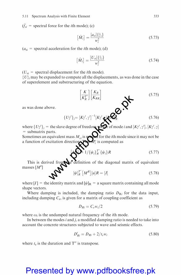
(�fsi = spectral force for the ith mode); (c)
~Mi
� ¼ asi½ � ~gif g
w2i
(5:73)
(asi = spectral acceleration for the ith mode); (d)
~Mi
� ¼ Usi½ � ~gif g
w2i
(5:74)
(Usi = spectral displacement for the ith mode).{U}imay be expanded to compute all the displacements, as was done in the caseof superelement and substructuring of the equation.
K
KT}R
� �KR
KRR
� �(5:75)
as was done above.
Ug0f gi¼ Kg0; g0½ ��1 Kg0; g½ � Uif gR (5:76)
where Ug0f gi =the slave degree of freedom vector ofmode i and Kg0; g0½ �, Kg0; g½ �= submatrix parts.Sometimes an equivalent massMei is needed for the ith mode since it may not bea function of excitation direction. This Me
i is computed as
Mei
� ¼ 1= cif g
T}R cif gR (5:77)
This is derived from the definition of the diagonal matrix of equivalentmasses [Me]
c½ �T}R MR�
u½ �R ¼ I½ � (5:78)
where [I ] = the identity matrix and [c]R= a square matrix containing all modeshape vectors.
Where damping is included, the damping ratio DRi for the data input,including damping Ce, is given for a matrix of coupling coefficient as
DRi ¼ Cewi=2 (5:79)
where oi is the undamped natural frequency of the ith mode.In between the modes i and j, a modified damping ratio is needed to take into
account the concrete structures subjected to wave and seismic effects.
D0Ri ¼ DRi þ 2=tewi (5:80)
where te is the duration and T00 is transpose.
5.11 Spectrum Analysis with Finite Element 333
www.pdfbo
oksfr
ee.pk
Presented by www.pdfbooksfree.pk
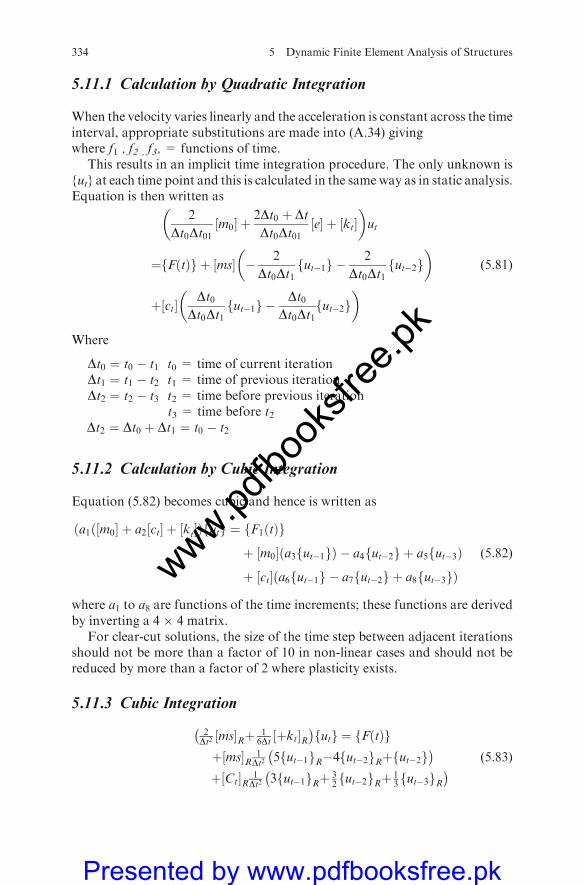
5.11.1 Calculation by Quadratic Integration
When the velocity varies linearly and the acceleration is constant across the timeinterval, appropriate substitutions are made into (A.34) givingwhere f1 , f2 , f3, = functions of time.
This results in an implicit time integration procedure. The only unknown is{ut} at each time point and this is calculated in the same way as in static analysis.Equation is then written as
2
Dt0Dt01m0½ � þ
2Dt0 þ DtDt0Dt01
e½ � þ kt½ �� �
ut
¼ FðtÞf g þ ms½ � � 2
Dt0Dt1ut�1f g � 2
Dt0Dt1ut�2f g
� �
þ ct½ �Dt0
Dt0Dt1ut�1f g � Dt0
Dt0Dt1ut�2f g
� �(5:81)
Where
Dt0 ¼ t0 � t1 t0 = time of current iterationDt1 ¼ t1 � t2 t1 = time of previous iterationDt2 ¼ t2 � t3 t2 = time before previous iteration
t3 = time before t2Dt2 ¼ Dt0 þ Dt1 ¼ t0 � t2
5.11.2 Calculation by Cubic Integration
Equation (5.82) becomes cubic and hence is written as
ða1ð½m0� þ a2½ct� þ ½kt�Þfutg ¼ fF1ðtÞg
þ ½m0�ða3fut�1gÞ � a4fut�2g þ a5fut�3Þ
þ ½ct�ða6fut�1g � a7fut�2g þ a8fut�3gÞ
(5:82)
where a1 to a8 are functions of the time increments; these functions are derivedby inverting a 4 � 4 matrix.
For clear-cut solutions, the size of the time step between adjacent iterationsshould not be more than a factor of 10 in non-linear cases and should not bereduced by more than a factor of 2 where plasticity exists.
5.11.3 Cubic Integration
2Dt2 ms½ �Rþ 1
6Dt þkt½ �R �
utf g ¼ FðtÞf gþ ms½ �R 1
Dt2 5 ut�1f gR�4 ut�2f gRþ ut�2f g �
þ Ct½ �R 1Dt2 3 ut�1f gRþ 3
2 ut�2f gRþ 13 ut�3f gR
� (5:83)
334 5 Dynamic Finite Element Analysis of Structures
www.pdfbo
oksfr
ee.pk
Presented by www.pdfbooksfree.pk
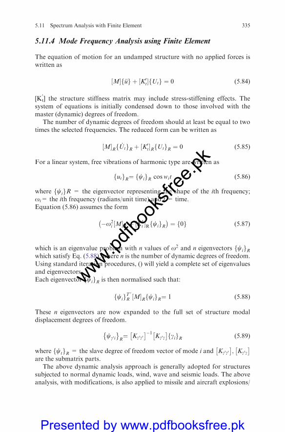
5.11.4 Mode Frequency Analysis using Finite Element
The equation of motion for an undamped structure with no applied forces iswritten as
½M�f€ug þ ½K0t�fUtg ¼ 0 (5:84)
[K0
t] the structure stiffness matrix may include stress-stiffening effects. Thesystem of equations is initially condensed down to those involved with themaster (dynamic) degrees of freedom.
The number of dynamic degrees of freedom should at least be equal to twotimes the selected frequencies. The reduced form can be written as
½M�Rf _UtgR þ ½K0t�RfUtgR ¼ 0 (5:85)
For a linear system, free vibrations of harmonic type are written as
utf gR¼ cif gR coswit (5:86)
where cif gR = the eigenvector representing the shape of the ith frequency;oi= the ith frequency (radians/unit time) and t = time.Equation (5.86) assumes the form
�o2i ½M�R þ ½K1
t �R cif gR �
¼ 0f g (5:87)
which is an eigenvalue problem with n values of o2 and n eigenvectors cif gRwhich satisfy Eq. (5.88), where n is the number of dynamic degrees of freedom.Using standard iteration procedures, () will yield a complete set of eigenvaluesand eigenvectors.Each eigenvector cif gR is then normalised such that:
cif gT}R M½ �R cif gR¼ 1 (5:88)
These n eigenvectors are now expanded to the full set of structure modaldisplacement degrees of freedom.
cg0i
� R¼ Kg0g0� �1
Kg0g�
gif gR (5:89)
where ctf gR = the slave degree of freedom vector of mode i and Kg0g0�
; Kg0g�
are the submatrix parts.The above dynamic analysis approach is generally adopted for structures
subjected to normal dynamic loads, wind, wave and seismic loads. The aboveanalysis, with modifications, is also applied to missile and aircraft explosions/
5.11 Spectrum Analysis with Finite Element 335
www.pdfbo
oksfr
ee.pk
Presented by www.pdfbooksfree.pk
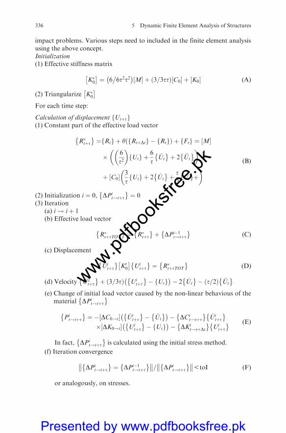
impact problems. Various steps need to included in the finite element analysisusing the above concept.Initialization(1) Effective stiffness matrix
K�0�
¼ 6 6t2�
t2 �
M½ � þ 3 3t= tð Þ C0½ � þ K0½ � (A)
(2) Triangularize K�0�
For each time step:
Calculation of displacement Utþtf g(1) Constant part of the effective load vector
R�tþt�
¼ Rtf g þ y RtþDtf g � Rtf gð Þ þ Ftf g ¼ M½ �
� 6
t2
� �Utf g þ 6
t_Ut
� þ 2 €Ut
� � �
þ C0½ �3
tUtf g þ 2 _Ut
� þ t2
Utf gþ� � (B)
(2) Initialization i ¼ 0, DPit!tþt
� ¼ 0
(3) Iteration(a) i! iþ 1(b) Effective load vector
R�tþtTOT
� ¼ R�tþt�
þ DPi�1t!tþt
� (C)
(c) Displacement
Uitþt
� K00�
Uitþt
� ¼ R�tþtTOT
� (D)
(d) Velocity U2tþt
� þ 3 3t=ð Þ Ui
tþt�
� Utf g �
� 2 _Ut
� � t=2ð Þ €Ut
� (e) Change of initial load vector caused by the non-linear behavious of the
material DPit!tþt
�
Pit!tþt
� ¼ � DC0!t½ � _Ui
tþt�
� _Ut
� �� DCi
t!tþt�
_Uitþt
� � DK0!t½ � Ui
tþt�
� Utf g �
� DKit!tþDt
� Ui
tþt� (E)
In fact, DPit!tþt
� is calculated using the initial stress method.
(f) Iteration convergence
DPit!tþt
� ¼ DPi�1
t!tþt� �� ��= DPi
t!tþt� �� ��5toI (F)
or analogously, on stresses.
336 5 Dynamic Finite Element Analysis of Structures
www.pdfbo
oksfr
ee.pk
Presented by www.pdfbooksfree.pk
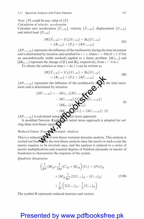
Note: Pf g could be any value of Ff g.Calculation of velocity, accelerationCalculate new acceleration €UtþDt
� , velocity _UtþDt
� , displacement UtþDtf g
and initial load PtþDtf g
½M�f €UtþDtg þ ½C0�fUtþDtg þ ½K0�fUtþDtg¼ fRtþDtg þ fPtg þ fDPt!tþDtg
(G)
fDPt!tþDtg represents the influence of the nonlinearity during the time incrementand is determined by iteration and satisfied for tþ t, where t ¼ yDt (y> 1.37 foran unconditionally stable method) applied to a linear problem. [DC0!t] and[DK0!t ] represent the change of [C] and [K], respectively, from t = 0 to t.
To obtain the solution at time tþ Dt, ( ) can be written as
½M�f €UtþDtg þ ½C0�fUtþDtg þ ½K0�fUtþDtg¼ fRtþDtg þ fFtg þ fDFt!tþDtg
(H)
DPt!tþDtf g represents the influence of the nonlinearity during the time incre-ment and is determined by iteration
fDPt!tþDtg ¼ � ½DC0!t�fDUt!tþDtg
� ½DCt!tþDt�ðfUg þ fDUt!tþDtgÞ
� ½DK0!t�fDUt!tþDtg
� ½DKt!tþDt�ðfUtg þ fDUt!tþDtgÞ ðIÞ
(I)
DPt!tþDtf g is calculated using the initial stress approach.A modified Newton–Raphson or initial stress approach is adopted for sol-
ving these non-linear equations.
Reduced Linear Transient Dynamic Analysis
This is a reduced form of non-linear transient dynamic analysis. This analysis iscarried out faster than the non-linear analysis since the matrix in such a case thematrix requires to be inverted once, and the analysis is reduced to a series ofmatrix multiplications and essential degrees of freedom (dynamic or master offreedoms) to characterize the response of the system.
Quadratic Integration
1
Dt2½M�R
�þ 3
2Dt½Ct�R þ ½Kt�R
�fUtg ¼ fFðtÞgR
þ ½M�R1
Dt22fUt�1gR � fUt�2gRð Þ
þ 1
Dt2fUt�1gR �
1
2fUt�2gR
� �(5:90)
The symbol R represents reduced matrices and vectors.
5.11 Spectrum Analysis with Finite Element 337
www.pdfbo
oksfr
ee.pk
Presented by www.pdfbooksfree.pk
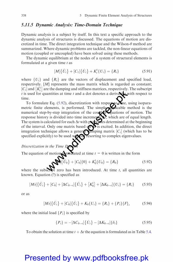
5.11.5 Dynamic Analysis: Time-Domain Technique
Dynamic analysis is a subject by itself. In this text a specific approach to thedynamic analysis of structures is discussed. The equations of motion are dis-cretized in time. The direct integration technique and the Wilson-y method aresummarized. Where dynamic problems are tackled, the non-linear equations ofmotion (coupled or uncoupled) have been solved using these methods.
The dynamic equilibrium at the nodes of a system of structural elements isformulated at a given time t as
M½ � €Ut
� þ C1½ � _Ut
� þ K1
t Utf g ¼ Rtf g (5:91)
where Utf g and Rtf g are the vectors of displacement and specified load,respectively. [M] represents the mass matrix which is regarded as constant;Ct½ � and K1
t
� are the damping and stiffness matrices, respectively. The subscript
t is used for quantities at time t and a dot denotes a derivative with respect totime.
To formulate Eq. (5.92), discretization with respect to time, using isopara-metric finite elements, is performed. The simple applicable method is thenumerical step-by-step integration of the coupled equations of motion. Theresponse history is divided into time increments Dt, which are of equal length.The system is calculated for eachDtwith properties determined at the beginningof the interval. Only one matrix based on M is excited. In addition, the directintegration technique allows a general damping matrix Ct½ � (which has to bespecified explicitly) to be used without resorting to complex eigenvalues.
Discretization in the Time Domain
The equation of motion formulated at time t = 0 is written in the form
M½ � €U0
� þ C0½ � 0f g þ K1
0 U0f g ¼ R0f g (5:92)
where the subscript zero has been introduced. At time t, all quantities areknown. Equation (?) is specified as
Ms½ � €Ut
� þ C0½ � þ DC0!t½ � €Ut
� þ K1
0
� þ DK0!t½ � Utf g ¼ Rtf g (5:93)
or as
Ms½ � €Ut
� þ C0½ � _Ut
� þ K0 Utf g ¼ Rtf g þ Ptf g Ff gt (5:94)
where the initial load Ptf g is specified by
Ptf g ¼ � DC0!t½ � _Ut
� � DK0!t½ � dtf g (5:95)
To obtain the solution at time tþ Dt the equation is formulated as in Table 5.4.
338 5 Dynamic Finite Element Analysis of Structures
www.pdfbo
oksfr
ee.pk
Presented by www.pdfbooksfree.pk
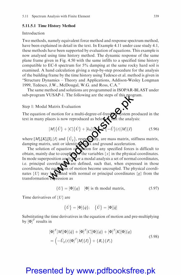
5.11.5.1 Time History Method
Introduction
Twomethods, namely equivalent force method and response spectrummethod,have been explained in detail in the text. In Example 4.11 under case study 4.1,these methods have been supported by evaluation of equations. This example isnow analysed using time history method. The dynamic response of the sameplane frame given in Fig. 4.50 with the same infills to a specified time historycompatible to EC-8 spectrum for 5% damping at the same rocky hard soil isexamined. A hand calculation giving a step-by-step procedure for the analysisof the building frame by the time history using Tedesco et al. method is given in‘‘Structure Dynamics – Theory and Applications, Addison-Wesley Longman1999, Tedesco, J.W., McDougal, W.G. and Ross, C.A.’’
The same method and solutions are programmed in ISOPAR-BLAST undersub-program VUSAP-1. The following are the steps of this program.
Step 1: Modal Matrix Evaluation
The equation of motion for a multi-degree-of-freedom system produced in thetext in many places is now reproduced as below to suit the analysis:
M½ � €U�
þ C½ � _U�
þ k0½ � Uf g ¼ � €U�
ðtÞM½ � If g (5:96)
where [M],[K],[I],{I} and €Ug
� , respectively, are mass matrix, stiffness matrix,
damping matrix, unit or identity matrix and ground acceleration.The solution of equation of motion for any specified forces is difficult to
obtain, mainly due to coupling of the variables {x} in the physical coordinates.In mode superposition analysis or a modal analysis a set of normal coordinates,i.e. principal coordinates, are defined, such that, when expressed in thosecoordinates, the equations of motion become uncoupled. The physical coordi-nates {U} may be related with normal or principal coordinates {g} from thetransformation expression as
Uf g ¼ F½ � qf g F½ � is th modal matrix, (5:97)
Time derivatives of {U} are
_U�
¼ F½ � _qf g; €U�
¼ F½ � €q½ �
Substituting the time derivatives in the equation of motion and pre-multiplyingby F½ �T results in
F½ �T M½ � F½ � €qf g þ F½ �T C½ � F½ � _qf g þ F½ �T K½ � F½ � qf g
¼ � €UgðtÞ F½ �T M½ � If g� �
þ Rtf g Ptf g(5:98)
5.11 Spectrum Analysis with Finite Element 339
www.pdfbo
oksfr
ee.pk
Presented by www.pdfbooksfree.pk
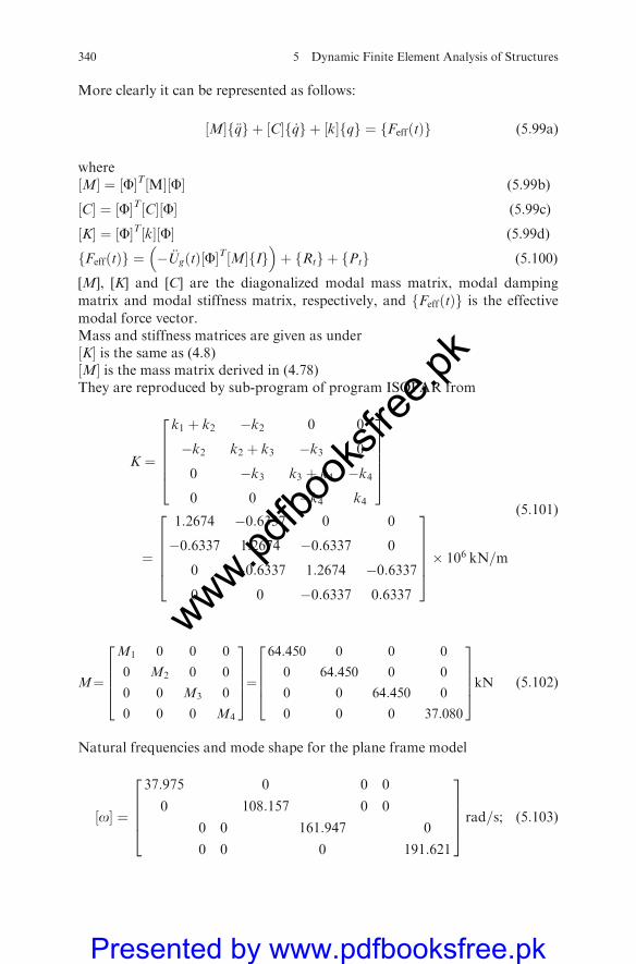
More clearly it can be represented as follows:
M½ � €qf g þ C½ � _qf g þ k½ � qf g ¼ FeffðtÞf g (5:99a)
whereM½ � ¼ F½ �T M½ � F½ � (5.99b)
C½ � ¼ F½ �T C½ � F½ � (5.99c)
K½ � ¼ F½ �T k½ � F½ � (5.99d)
FeffðtÞf g ¼ � €UgðtÞ F½ �T M½ � If g� �
þ Rtf g þ Ptf g (5.100)
[M], [K] and [C] are the diagonalized modal mass matrix, modal damping
matrix and modal stiffness matrix, respectively, and FeffðtÞf g is the effective
modal force vector.Mass and stiffness matrices are given as underK½ � is the same as (4.8)M½ � is the mass matrix derived in (4.78)They are reproduced by sub-program of program ISOPAR from
K ¼
k1 þ k2 �k2 0 0
�k2 k2 þ k3 �k3 0
0 �k3 k3 þ k4 �k40 0 �k4 k4
266664
377775
¼
1:2674 �0:6337 0 0
�0:6337 1:2674 �0:6337 0
0 �0:6337 1:2674 �0:63370 0 �0:6337 0:6337
266664
377775� 106 kN=m
(5:101)
M¼
M1 0 0 0
0 M2 0 0
0 0 M3 0
0 0 0 M4
26664
37775¼
64:450 0 0 0
0 64:450 0 0
0 0 64:450 0
0 0 0 37:080
26664
37775kN (5:102)
Natural frequencies and mode shape for the plane frame model
o½ � ¼
37:975 0
0 108:157
0 0
0 0
0 0
0 0
161:947 0
0 191:621
26664
37775 rad=s; (5:103)
340 5 Dynamic Finite Element Analysis of Structures
www.pdfbo
oksfr
ee.pk
Presented by www.pdfbooksfree.pk
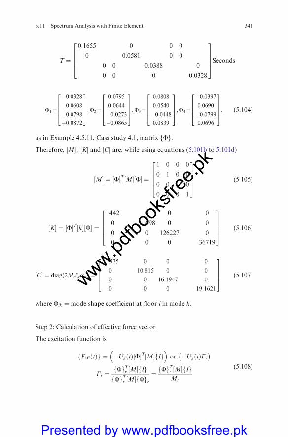
T ¼
0:1655 0
0 0:0581
0 0
0 0
0 0
0 0
0:0388 0
0 0:0328
26664
37775Seconds
F1¼
�0:0328�0:0608�0:0798�0:0872
26664
37775;F2¼
0:0795
0:0644
�0:0273�0:0865
26664
37775;F3¼
0:0808
0:0540
�0:04480:0839
26664
37775;F4¼
�0:03970:0690
�0:07990:0696
26664
37775; (5:104)
as in Example 4.5.11, Cass study 4.1, matrix Ff g.
Therefore, M½ �; K½ � and C½ � are, while using equations (5.101b to 5.101d)
M½ � ¼ F½ �T M½ � F½ � ¼
1 0 0 0
0 1 0 0
0 0 1 0
0 0 0 1
26664
37775 (5:105)
K½ � ¼ F½ �T k½ � F½ � ¼
1442 0
0 11698
0 0
0 0
0 0
0 0
126227 0
0 36719
26664
37775 (5:106)
C½ � ¼ diag 2Mrzrorð Þ ¼
3:7975 0
0 10:815
0 0
0 0
0 0
0 0
16:1947 0
0 19:1621
26664
37775 (5:107)
where Fik ¼ mode shape coefficient at floor i in mode k.
Step 2: Calculation of effective force vector
The excitation function is
FeffðtÞf g ¼ � €UgðtÞ F½ �T M½ � If g� �
or � €UgðtÞGr
�
Gr ¼Ff gTr M½ � If gFf gTr M½ � Ff gr
¼ Ff gTr M½ � If gMr
(5:108)
5.11 Spectrum Analysis with Finite Element 341
www.pdfbo
oksfr
ee.pk
Presented by www.pdfbooksfree.pk
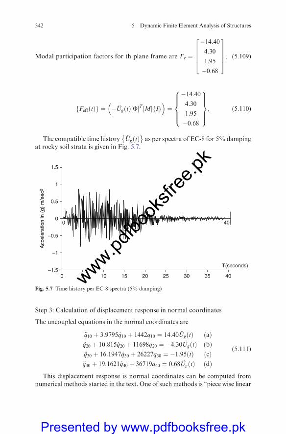
Modal participation factors for th plane frame are Gr ¼
�14:404:30
1:95
�0:68
26664
37775; (5:109)
FeffðtÞf g ¼ � €UgðtÞ F½ �T M½ � If g� �
¼
�14:404:30
1:95
�0:68
8>>><>>>:
9>>>=>>>;; (5:110)
The compatible time history €UgðtÞ�
as per spectra of EC-8 for 5% dampingat rocky soil strata is given in Fig. 5.7.
Step 3: Calculation of displacement response in normal coordinates
The uncoupled equations in the normal coordinates are
€q10 þ 3:9795 _q10 þ 1442q10 ¼ 14:40 €UgðtÞ að Þ€q20 þ 10:815 _q20 þ 11698q20 ¼ �4:30 €UgðtÞ bð Þ€q30 þ 16:1947 _q30 þ 26227q30 ¼ �1:95ðtÞ cð Þ€q40 þ 19:1621 _q40 þ 36719q40 ¼ 0:68 €UgðtÞ dð Þ
(5:111)
This displacement response is normal coordinates can be computed fromnumerical methods started in the text. One of such methods is ‘‘piece wise linear
50–1.5
–1
–0.5
Acc
eler
atio
n in
(g)
m/s
ec2
0
0.5
1.5
1
10 15
0 40
20 25 30 35 40
T(seconds)
Fig. 5.7 Time history per EC-8 spectra (5% damping)
342 5 Dynamic Finite Element Analysis of Structures
www.pdfbo
oksfr
ee.pk
Presented by www.pdfbooksfree.pk
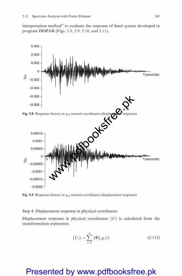
interpretation method’’ to evaluate the response of lined system developed in
program ISOPAR (Figs. 5.8, 5.9, 5.10, and 5.11).
Step 4: Displacement response in physical coordinates
Displacement response in physical coordinates {U} is calculated from the
transformation expression.
Utf g ¼Xnr¼1
Ff grqrðtÞ (5:112)
0
0.002
–0.002q 10
–0.004
–0.006
–0.008
0.004
0.005
T(seconds)
Fig. 5.8 Response history in q10 normal coordinates (displacement response)
00
0.00005
–0.00005
q 20
–0.0001
–0.00015
–0.0002
0.0001
0.00015
T(seconds)
Fig. 5.9 Response history in q20 normal coordinates (displacement response)
5.11 Spectrum Analysis with Finite Element 343
www.pdfbo
oksfr
ee.pk
Presented by www.pdfbooksfree.pk
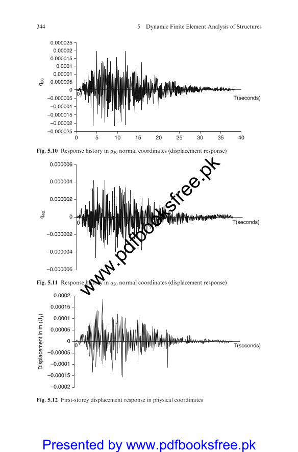
T(seconds)
–0.000006
–0.000004
0.000004
0.000006
–0.000002
0.000002
00
q 40
Fig. 5.11 Response history in q20 normal coordinates (displacement response)
–0.0002
–0.0001
–0.00015
0.00015
0.0002
–0.00005
0.0001
0.00005
00
Dis
plac
emen
t in
m (
U1)
T(seconds)
Fig. 5.12 First-storey displacement response in physical coordinates
50 10 15 20 25 30 35 40
T(seconds)
00
–0.00001
0.0001
0.00001
–0.000005
0.000005q 30
–0.000015
0.000015
–0.00002
0.00002
–0.000025
0.000025
Fig. 5.10 Response history in q30 normal coordinates (displacement response)
344 5 Dynamic Finite Element Analysis of Structures
www.pdfbo
oksfr
ee.pk
Presented by www.pdfbooksfree.pk
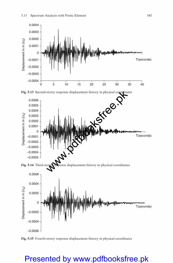
0–0.0004
–0.0003
–0.0002
–0.0001
0.0001
0.0002
0.0003
0.0004
0
5 10 15 20 25 35 40
T(seconds)
30
Dis
plac
emen
t in
m (
U2)
Fig. 5.13 Second-storey response displacement history in physical coordinates
–0.0005
–0.0004
–0.0003
–0.0002
–0.0001
0.0001
0.0002
0.0003
0.0005
0.0004
0.0006
0
Dis
plac
emen
t in
m (
U3)
T(seconds)
Fig. 5.14 Third-storey response displacement history in physical coordinates
–0.0006
–0.0004
–0.0002
0.0002
0.0004
0.0006
0
Dis
plac
emen
t in
m (
U4)
T(seconds)
Fig. 5.15 Fourth-storey response displacement history in physical coordinates
5.11 Spectrum Analysis with Finite Element 345
www.pdfbo
oksfr
ee.pk
Presented by www.pdfbooksfree.pk
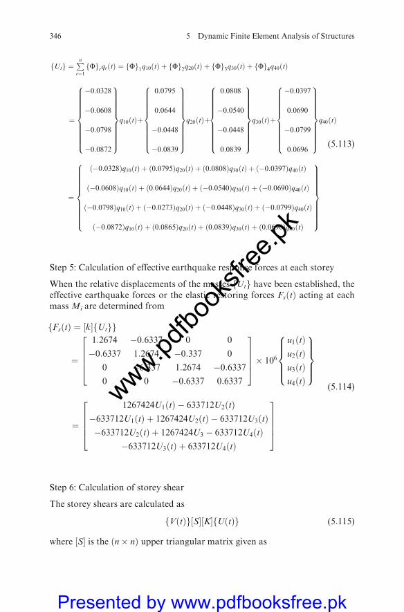
Utf g ¼Pnr¼1
Ff grqrðtÞ ¼ Ff g1q10ðtÞ þ Ff g2q20ðtÞ þ Ff g3q30ðtÞ þ Ff g4q40ðtÞ
¼
�0:0328
�0:0608
�0:0798
�0:0872
8>>>>>>>>><>>>>>>>>>:
9>>>>>>>>>=>>>>>>>>>;
q10ðtÞþ
0:0795
0:0644
�0:0448
�0:0839
8>>>>>>>>><>>>>>>>>>:
9>>>>>>>>>=>>>>>>>>>;
q20ðtÞþ
0:0808
�0:0540
�0:0448
0:0839
8>>>>>>>>><>>>>>>>>>:
9>>>>>>>>>=>>>>>>>>>;
q30ðtÞþ
�0:0397
0:0690
�0:0799
0:0696
8>>>>>>>>><>>>>>>>>>:
9>>>>>>>>>=>>>>>>>>>;
q40ðtÞ
¼
�0:0328ð Þq10ðtÞ þ 0:0795ð Þq20ðtÞ þ 0:0808ð Þq30ðtÞ þ �0:0397ð Þq40ðtÞ
�0:0608ð Þq10ðtÞ þ 0:0644ð Þq20ðtÞ þ �0:0540ð Þq30ðtÞ þ �0:0690ð Þq40ðtÞ
�0:0798ð Þq10ðtÞ þ �0:0273ð Þq20ðtÞ þ �0:0448ð Þq30ðtÞ þ �0:0799ð Þq40ðtÞ
�0:0872ð Þq10ðtÞ þ 0:0865ð Þq20ðtÞ þ 0:0839ð Þq30ðtÞ þ 0:0696ð Þq40ðtÞ
8>>>>>>>>><>>>>>>>>>:
9>>>>>>>>>=>>>>>>>>>;
(5:113)
Step 5: Calculation of effective earthquake response forces at each storey
When the relative displacements of the masses Utf g have been established, theeffective earthquake forces or the elastic restoring forces FsðtÞ acting at eachmass Mi are determined from
FsðtÞ ¼ k½ � Utf gf g
¼
1:2674 �0:6337 0 0
�0:6337 1:2674 �0:337 0
0 �6:337 1:2674 �0:63370 0 �0:6337 0:6337
26664
37775� 106
u1ðtÞu2ðtÞu3ðtÞu4ðtÞ
8>>><>>>:
9>>>=>>>;
¼
1267424U1ðtÞ � 633712U2ðtÞ�633712U1ðtÞ þ 1267424U2ðtÞ � 633712U3ðtÞ�633712U2ðtÞ þ 1267424U3 � 633712U4ðtÞ
�633712U3ðtÞ þ 633712U4ðtÞ
26664
37775
(5:114)
Step 6: Calculation of storey shear
The storey shears are calculated as
VðtÞf g S½ � K½ � UðtÞf g (5:115)
where S½ � is the n� nð Þ upper triangular matrix given as
346 5 Dynamic Finite Element Analysis of Structures
www.pdfbo
oksfr
ee.pk
Presented by www.pdfbooksfree.pk
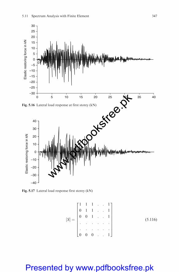
S½ � ¼
1 1 1 : : 1
0 1 1 : : 1
0 0 1 : : 1
: : : : : :
: : : : : :
0 0 0 : : 1
2666666664
3777777775
(5:116)
–3050 10 15 20 25 35 4030
–25
–15
Ela
stic
res
torin
g fo
rce
in k
N
–5
5
10
20
30
25
15
00
–20
–10
Fig. 5.16 Lateral load response at first storey (kN)
00
–10
10
–20
20
–30
30
–40
40
Ela
stic
res
torin
g fo
rce
in k
N
Fig. 5.17 Lateral load response first storey (kN)
5.11 Spectrum Analysis with Finite Element 347
www.pdfbo
oksfr
ee.pk
Presented by www.pdfbooksfree.pk
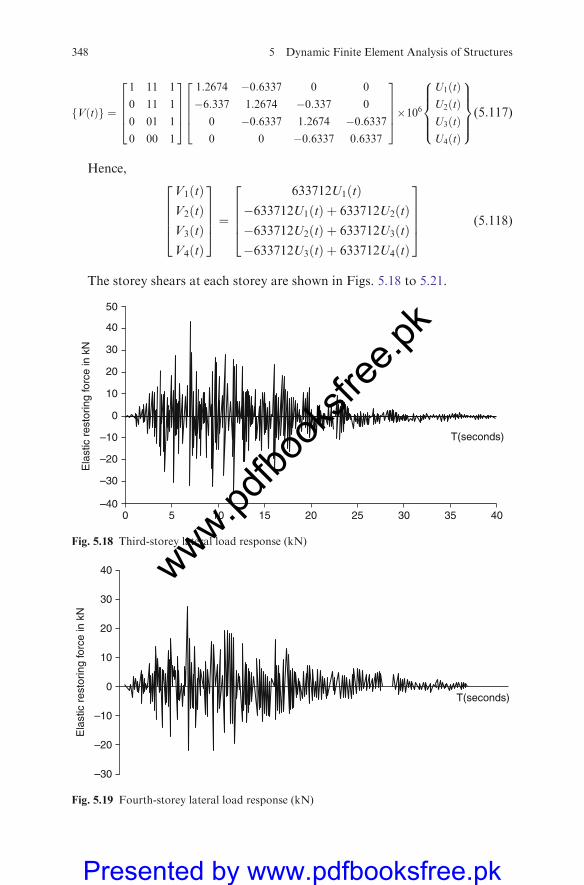
VðtÞf g ¼
1 11 1
0 11 1
0 01 1
0 00 1
26664
37775
1:2674 �0:6337 0 0
�6:337 1:2674 �0:337 0
0 �0:6337 1:2674 �0:63370 0 �0:6337 0:6337
26664
37775�106
U1ðtÞU2ðtÞU3ðtÞU4ðtÞ
8>>><>>>:
9>>>=>>>;(5:117)
Hence,
V1ðtÞV2ðtÞV3ðtÞV4ðtÞ
26664
37775 ¼
633712U1ðtÞ�633712U1ðtÞ þ 633712U2ðtÞ�633712U2ðtÞ þ 633712U3ðtÞ�633712U3ðtÞ þ 633712U4ðtÞ
26664
37775 (5:118)
The storey shears at each storey are shown in Figs. 5.18 to 5.21.
0–40
40
50
–30
30
–20
20
–10
10
0
5 10 20 3015 25 35 40
T(seconds)
Ela
stic
res
torin
g fo
rce
in k
N
Fig. 5.18 Third-storey lateral load response (kN)
40
–30
30
–20
20
–10
10
0
Ela
stic
res
torin
g fo
rce
in k
N
T(seconds)
Fig. 5.19 Fourth-storey lateral load response (kN)
348 5 Dynamic Finite Element Analysis of Structures
www.pdfbo
oksfr
ee.pk
Presented by www.pdfbooksfree.pk
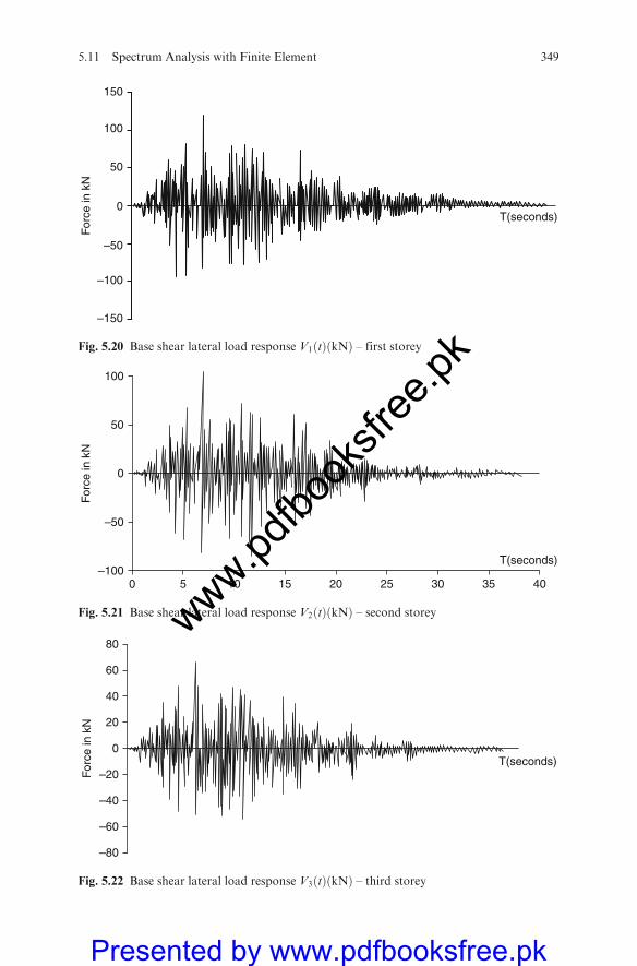
150
100
50
–50
For
ce in
kN
–100
–150
0T(seconds)
Fig. 5.20 Base shear lateral load response V1ðtÞðkNÞ – first storey
0–100
–50
For
ce in
kN
0
50
100
5 10 20 30 40
T(seconds)
25 3515
Fig. 5.21 Base shear lateral load response V2ðtÞðkNÞ – second storey
For
ce in
kN
–80
80
–40
40
–20
20
–60
60
0T(seconds)
Fig. 5.22 Base shear lateral load response V3ðtÞðkNÞ – third storey
5.11 Spectrum Analysis with Finite Element 349
www.pdfbo
oksfr
ee.pk
Presented by www.pdfbooksfree.pk
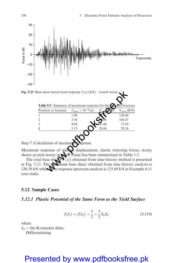
Step 7: Calculation of maximum response
Maximum response of relative displacement, elastic restoring forces, storeyshears at each storey in plane frame has been summarized in Table 5.5.
The total base shears V1ðtÞ obtained from time history method is presentedin Fig. 5.23. The maximum base shear obtained from time history analysis is120.39 kN while from response spectrum analysis is 125.69 kN in Example 4.11case study.
5.12 Sample Cases
5.12.1 Plastic Potential of the Same Form as the Yield Surface
f J2ð Þ ¼ f dij �
¼ 3
2¼ 3
2SijSij (5:119)
wheredij ¼ the Kronecker delta.
Differentiating
T(seconds)
For
ce in
kN
–20
20
–10
10
–30
30
0
Fig. 5.23 Base shear lateral load response V4ðtÞðkNÞ – fourth storey
Table 5.5 Summary of maximum response for the example structure
Position or location Umax � 10�4ðmÞ Fmax (KN) Vmax (KN)
1 1.90 23.4 120.40
2 3.54 32.88 104.47
3 4.68 43.86 72.10
4 5.13 28.64 28.24
350 5 Dynamic Finite Element Analysis of Structures
www.pdfbo
oksfr
ee.pk
Presented by www.pdfbooksfree.pk
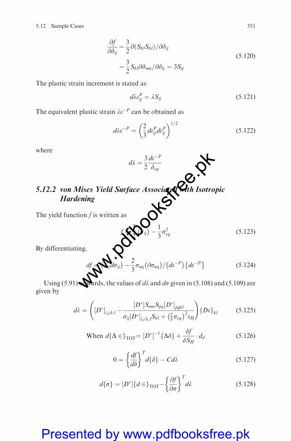
@f
@dij¼ 3
2@ SklSklð Þ=@dij
¼ 3
2Skl@dmn=@dij ¼ 3Sij
(5:120)
The plastic strain increment is stated as
dlePij ¼ lSij (5:121)
The equivalent plastic strain le�P can be obtained as
dle�P ¼ 2
3dePij de
Pij
� �1=2
(5:122)
where
dl ¼ 3
2
de�P
deq
5.12.2 von Mises Yield Surface Associated with IsotropicHardening
The yield function f is written as
f ¼ T
2sij �
� 1
3s2eq (5:123)
By differentiating,
df ¼ Sijdsij
�� 2
3seq @seq �
= de�P �
de�P�
(5:124)
Using (5.91) onwards, the values of dl and ds given in (5.108) and (5.109) aregiven by
dl ¼ D�½ �i;j;k;l�D�½ �SmnSpq D
�½ �pqklsij D�½ �i:j:k;lSkl þ 2
3seq �2
sH
!Def gkl (5:125)
When d D 2f gTOT¼ D�½ ��1 Ddf g þ dfdSH� dd (5:126)
0 ¼ df
dd
� �T
d df g � Cdl (5:127)
d sf g ¼ D�½ � d 2f gTOT�@f
@s
� �T
dl (5:128)
5.12 Sample Cases 351
www.pdfbo
oksfr
ee.pk
Presented by www.pdfbooksfree.pk
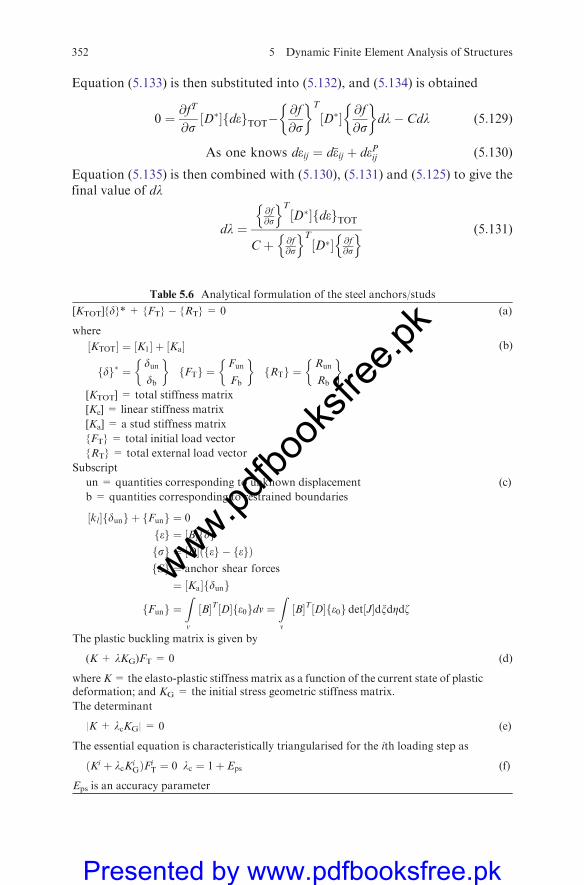
Equation (5.133) is then substituted into (5.132), and (5.134) is obtained
0 ¼ @fT
@sD�½ � def gTOT�
@f
@s
� �T
D�½ � @f
@s
� �dl� Cdl (5:129)
As one knows deij ¼ d�eij þ dePij (5:130)
Equation (5.135) is then combined with (5.130), (5.131) and (5.125) to give thefinal value of dl
dl ¼@f@s
n oT
D�½ � def gTOT
Cþ @f@s
n oT
D�½ � @f@s
n o (5:131)
Table 5.6 Analytical formulation of the steel anchors/studs
[KTOT]{d}* + {FT} � {RT} = 0 (a)
where
½KTOT� ¼ ½K1� þ ½Ka�
fdg� ¼dundb
� �fFTg ¼
Fun
Fb
� �fRTg ¼
Run
Rb
� � (b)
[KTOT] = total stiffness matrix
[Ke] = linear stiffness matrix
[Ka] = a stud stiffness matrix
{FT} = total initial load vector
{RT} = total external load vector
Subscript
un = quantities corresponding to unknown displacement
b = quantities corresponding to restrained boundaries
(c)
½kl�fdung þ fFung ¼ 0
feg ¼ ½B�fdgfsg ¼ ½D�ðfeg � fegÞfSg ¼ anchor shear forces
¼ ½Ka�fdung
fFung ¼Zv
½B�T½D�fe0gdv ¼Zv
½B�T½D�fe0g det½J�dxdZdz
The plastic buckling matrix is given by
(K + lKG)FT = 0 (d)
where K= the elasto-plastic stiffness matrix as a function of the current state of plasticdeformation; and KG = the initial stress geometric stiffness matrix.
The determinant
|K + lcKG| = 0 (e)
The essential equation is characteristically triangularised for the ith loading step as
ðKi þ lcKiGÞFi
T ¼ 0 lc ¼ 1þ Eps (f)
Eps is an accuracy parameter
352 5 Dynamic Finite Element Analysis of Structures
www.pdfbo
oksfr
ee.pk
Presented by www.pdfbooksfree.pk
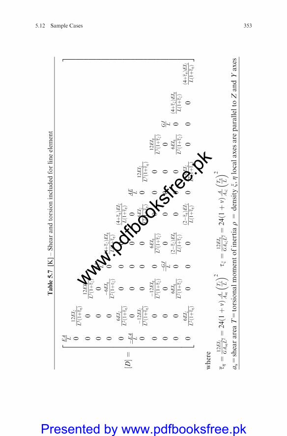
Table5.7
[K]–Shearandtorsionincluded
forlineelem
ent
½D�¼
EA L 0
12EI x
L3ð1þt ZÞ
00
12EI x
L3ð1þt xÞ
00
0GJ L
00
�6EI Z
L2ð1þt xÞ
0ð4þt xÞE
I ZLð1þt ZÞ
06EI x
L2ð1þt ZÞ
00
0ð4þt ZÞE
I xLð1þt ZÞ
�EA
L0
00
00
AE L
0�12EI x
L3ð1þt ZÞ
00
0�6EI x
L2ð1þt ZÞ
012EI x
L3ð1þt ZÞ
00
�12EI Z
L3ð1þt xÞ
06EI Z
L2ð1þt xÞ
00
012EI Z
L3ð1þt xÞ
00
0�GJ
L0
00
00
GJ L
00
6EI Z
L2ð1þt xÞ
0ð2�t xÞE
I ZLð1þt xÞ
00
06EI Z
L2ð1þt xÞ
0ð4þt xÞE
I ZLð1þt xÞ
06EI x
L2ð1þt ZÞ
00
0ð2�t ZÞE
I xLð1þt ZÞ
0�6EI x
L2ð1þt ZÞ
00
0ð4þt ZÞE
I xLð1þt ZÞ
2 6 6 6 6 6 6 6 6 6 6 6 6 6 6 6 6 6 6 6 6 6 6 6 6 6 4
3 7 7 7 7 7 7 7 7 7 7 7 7 7 7 7 7 7 7 7 7 7 7 7 7 7 5
where
t Z¼
12EI x
GA
sZL2¼
24ð1þnÞ
A AsZ
Tx L�� 2
t x¼
12EI Z
GA
sxL2¼
24ð1þnÞ
A Asx
TZ L�� 2
as=
shearareaT=torsionalmomentofinertiar=
density
x,Zlocalaxes
are
parallelto
ZandYaxes
5.12 Sample Cases 353
www.pdfbo
oksfr
ee.pk
Presented by www.pdfbooksfree.pk
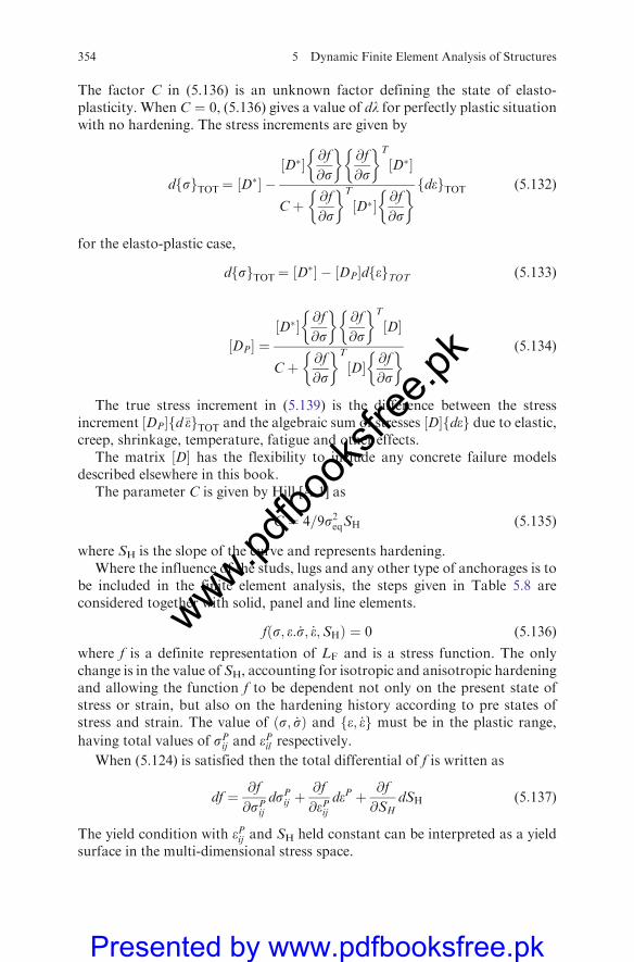
The factor C in (5.136) is an unknown factor defining the state of elasto-plasticity. When C ¼ 0, (5.136) gives a value of dl for perfectly plastic situationwith no hardening. The stress increments are given by
d sf gTOT¼ D�½ � �D�½ � @f
@s
� �@f
@s
� �T
D�½ �
Cþ @f
@s
� �T
D�½ � @f
@s
� � def gTOT (5:132)
for the elasto-plastic case,
d sf gTOT¼ ½D�� � ½DP�dfegTOT (5:133)
DP½ � ¼D�½ � @f
@s
� �@f
@s
� �T
D½ �
Cþ @f
@s
� �T
D½ � @f
@s
� � (5:134)
The true stress increment in (5.139) is the difference between the stressincrement DP½ � d�ef gTOT and the algebraic sum of stresses D½ � def g due to elastic,creep, shrinkage, temperature, fatigue and other effects.
The matrix D½ � has the flexibility to include any concrete failure modelsdescribed elsewhere in this book.
The parameter C is given by Hill [A.1] as
C ¼ 4=9s2eqSH (5:135)
where SH is the slope of the curve and represents hardening.Where the influence of the studs, lugs and any other type of anchorages is to
be included in the finite element analysis, the steps given in Table 5.8 areconsidered together with solid, panel and line elements.
f s; e: _s; _e;SHð Þ ¼ 0 (5:136)
where f is a definite representation of LF and is a stress function. The onlychange is in the value of SH, accounting for isotropic and anisotropic hardeningand allowing the function f to be dependent not only on the present state ofstress or strain, but also on the hardening history according to pre states ofstress and strain. The value of s; _sð Þ and e; _ef g must be in the plastic range,
having total values of sPij and ePil respectively.When (5.124) is satisfied then the total differential of f is written as
df ¼ @f
@sPijdsPij þ
@f
@ePijdeP þ @f
@SHdSH (5:137)
The yield condition with ePij and SH held constant can be interpreted as a yieldsurface in the multi-dimensional stress space.
354 5 Dynamic Finite Element Analysis of Structures
www.pdfbo
oksfr
ee.pk
Presented by www.pdfbooksfree.pk

When f< 0 the condition indicates a purely elastic change towards the insideof the yield surface. In cases where plastic flow does not occur, the increments ofplastic strain dePij and the change of hardening parameter dSH will be automa-tically zero, and hence, in the case of the unloading, (5.125) is reduced to
df ¼ @f
@sPijd sPijn o
50 (5:138)
When df ¼ 0, which is the case for neutral loading, no plastic strain changesoccur and the hardening factor remains unchanged, then
df ¼ @f
@sPijd sPijn o
¼ 0 d ePijn o
¼ 0 (5:139)
The quantity dsij is tangent to the surface for neutral loading. For the vectorproducts to be zero, @f=@sij will be normal to the surface. When dsij is pointing
Table 5.8 Stiffness coefficient and matrix for ISOPAR
The element pressure load vector in element coordinates is:fFPr
1 g ¼ P1 P2 P3 P4 P5 P6b cT
Value of stress stiffness coefficient (C2)
Previous iteration resulted in atensile stress
Previous iteration resulted in acompressive stress
1.0 0.0
1.0AE
F� 106
0.0 1.0AE
F� 1061.0
F ¼
for the first iteration : AEein
for all subsequent iterations : the axial forcein the element as computed in the previousstress pass of the element ðoutput quantityÞFORC
8>>>><>>>>:
C2 = value given in the table above.
The matrix for the tension-only or compression-only ISOPAR is given by:
M1½ � ¼Mt2
10 10 0 10 0 0 00 0 0 0 0 Symmetric0 0 0 0 0 00 0 0 0 0 0 10 0 0 0 0 0 0 10 0 0 0 0 0 0 0 10 0 0 0 0 0 0 0 0 00 0 0 0 0 0 0 0 0 0 00 0 0 0 0 0 0 0 0 0 0 0
26666666666666666664
37777777777777777775
5.12 Sample Cases 355
www.pdfbo
oksfr
ee.pk
Presented by www.pdfbooksfree.pk
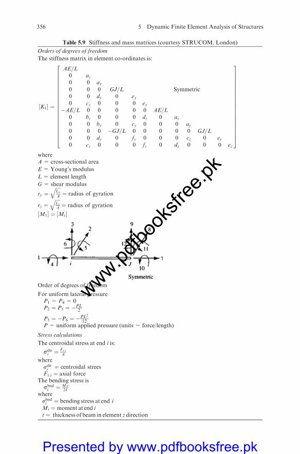
Table 5.9 Stiffness and mass matrices (courtesy STRUCOM, London)
Orders of degrees of freedom
The stiffness matrix in element co-ordinates is:
½K1� ¼
AE=L0 az0 0 ay0 0 0 GJ=L Symmetric0 0 dy 0 ey0 cz 0 0 0 ey
�AE=L 0 0 0 0 0 AE=L0 bz 0 0 0 dz 0 az0 0 by 0 cy 0 0 0 ay0 0 0 �GJ=L 0 0 0 0 0 GJ=L0 0 dy 0 fy 0 0 0 cz 0 ey0 cz 0 0 0 fz 0 dz 0 0 0 ez
26666666666666666664
37777777777777777775
whereA = cross-sectional area
E = Young’s modulus
L = element length
G = shear modulus
ry ¼ffiffiffiffiIyyA
q¼ radius of gyration
rz ¼ffiffiffiffiIzzA
q¼ radius of gyration
½M1� ¼ ½Mt�
Order of degrees of freedom
For uniform lateral pressureP1 = P4 = 0P2 ¼ P5 ¼ �PL
2
P3 ¼ �P6 ¼ �PL2
12P = uniform applied pressure (units = force/length)
Stress calculations
The centroidal stress at end i is:
sdiri ¼
Fx;i
A
wheresdiri ¼ centroidal streesFx;i ¼ axial force
The bending stress issbndi ¼ Mit
2Iwheresbndi ¼ bending stress at end iMi ¼ moment at end it ¼ thickness of beam in element zdirection
356 5 Dynamic Finite Element Analysis of Structures
www.pdfbo
oksfr
ee.pk
Presented by www.pdfbooksfree.pk
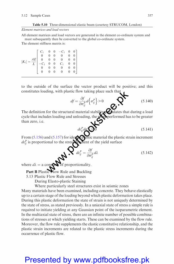
to the outside of the surface the vector product will be positive; and thisconstitutes loading, with plastic flow taking place such that
df ¼ @f
@sPijd sPijn o
40 (5:140)
The definition for the structural material stability postulates that during a loadcycle that includes loading and unloading, the work performed has to be greaterthan zero, i.e.
dePij dsPij � 0 (5:141)
From (5.156) and (5.157) for ideally plastic material the plastic strain incrementdePij is proportional to the stress gradient of the yield surface
dePij ¼@f
@sPijdl (5:142)
where dl ¼ a constant of proportionality.
Part B Plastic Flow Rule and Buckling5.13 Plastic Flow Rule and Stresses
During Elasto-plastic StainingWhere particularly steel structures exist in seismic zones
Many materials have been examined, including concrete. They behave elasticallyup to a certain stage of the loading beyondwhich plastic deformation takes place.During this plastic deformation the state of strain is not uniquely determined bythe state of stress, as stated previously. In a uniaxial state of stress a simple rule isrequired to initiate yielding at any Gaussian point of the isoparametric element.In the multiaxial state of stress, there are an infinite number of possible combina-tions of stresses at which yielding starts. These can be examined by the flow rule.Moreover, the flow rule supplements the elastic constitutive relationship, and theplastic strain increments are related to the plastic stress increments during theoccurrence of plastic flow.
Table 5.10 Three-dimensional elastic beam (courtesy STRUCOM, London)
Element matrices and load vectors
All element matrices and load vectors are generated in the element co-ordinate system andmust subsequently then be converted to the global co-ordinate system.
The element stiffness matrix is:
K1½ � ¼AE
L
C1 0 0 �C1 0 00 0 0 0 0 00 0 0 0 0 0�C1 0 0 C1 0 00 0 0 0 0 00 0 0 0 0 0
26666664
37777775
5.12 Sample Cases 357
www.pdfbo
oksfr
ee.pk
Presented by www.pdfbooksfree.pk

The yield criterion described by a failure surface in amulti-dimensional stress
space is given by Bangash:
LF sSij ;2P;SH
� �¼ 0 (5:143)
where
LF ¼ the yield functiontsSij ¼ the multi-dimensional stress state2P¼ accumulated plastic strainSH ¼ strain hardening or softening parameter
The general form of the yield surface given by (5.121) allows either isotropic
or kinematic hardening of the material. For a given previous history, LF sSij� �
is
Table 5.11 Two-dimensional elastic beam (courtesy STRUCOM,London)
Element matrices and load vectors
The element stiffness matrix in element co-ordinates is:
K1½ � ¼
AEL 0 0 �AE
L 0 0
0 12EIL3ð1þ f0Þ
6EIL2ð1þ f0Þ 0 � 12EI
L3ð1þ f0Þ6EI
Lð1þ f0Þ
0 6EIL2ð1þ f0Þ
EIð4þ f0ÞLð1þ f0Þ 0 � 6EI
L2ð1þ f0ÞEIð2� f0ÞLð1þ f0Þ
�AEL 0 0 AE
L 0 0
0 � 12EIL3ð1þ f0Þ
6EIL2ð1þ f0Þ 0 12EI
L3ð1þ f0Þ � 6EIL2ð1þ f0Þ
0 6EIL2ð1þ f0Þ
EIð2� f0ÞLð1þ f0Þ 0 � 6EI
L2ð1þ f0ÞEIð4þ f0ÞLð1þ f0Þ
2666666666666666664
3777777777777777775
whereA = cross-sectional areaE = Young’s modulusL = element lengthI = moment of inertiaf0 ¼ 12EI
GAsL2
G = shear modulusAs ¼ A
F s ¼ shear areaF s ¼ shear deflection constant
Two-dimensional beam element centroidal axis
358 5 Dynamic Finite Element Analysis of Structures
www.pdfbo
oksfr
ee.pk
Presented by www.pdfbooksfree.pk
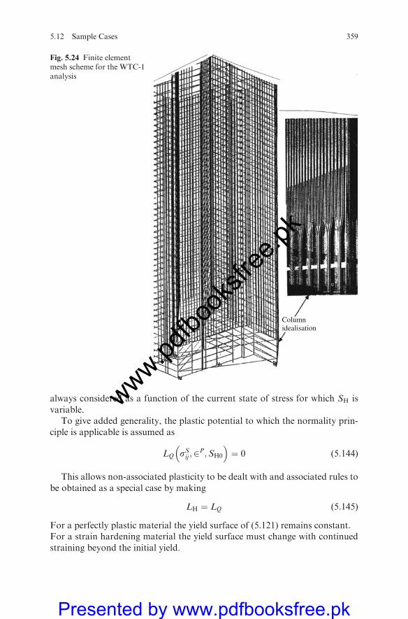
always considered as a function of the current state of stress for which SH isvariable.
To give added generality, the plastic potential to which the normality prin-ciple is applicable is assumed as
LQ sSij ;2P;SH0
� �¼ 0 (5:144)
This allows non-associated plasticity to be dealt with and associated rules tobe obtained as a special case by making
LH ¼ LQ (5:145)
For a perfectly plastic material the yield surface of (5.121) remains constant.For a strain hardening material the yield surface must change with continuedstraining beyond the initial yield.
Columnidealisation
Fig. 5.24 Finite elementmesh scheme for the WTC-1analysis
5.12 Sample Cases 359
www.pdfbo
oksfr
ee.pk
Presented by www.pdfbooksfree.pk
This phenomenon is included in (5.121) by allowing both LF and SH to befunctions of the state of stress and the plastic deformation history. This meansSH will have a new value for every time-dependent yielding. Further, if thematerial is unloaded and then loaded again, additional yielding cannot takeplace, unless the current value of SH has been exceeded.
A unified approach for arriving at the incremental stress–strain equationbased on (5.121) can be written in a combined tensor form in three dimensionsas the overall matrix is stored in the half-band form. Since the number ofdegrees of freedom is 15 at each story the dimensions of the stored matrix willbe (15�NS) by 30. The solution is obtained for the required number of loadingcases and from the displacements thus obtained and the generalized memberstiffness matrices. The stress resultants are found. Finally, the global load,stiffness and displacement relationships are obtained for the overall structures.
5.12.3 Dynamic Local and Global Stability Analysis
When the impact/blast occurs, there can be problem of combined torsional–flexural buckling of the building comprising the core, floors, columns andbracings. The elements of the building structures may be bolted or welded or incase of concrete connected with bars embedded to floors. The torsional bucklinganalysis can be combined with flexural buckling by adjusting the respectivestiffness matrices. The torsional buckling was dealt with in detail already.
5.12.3.1 Dynamic Flexural Buckling
The eigenvalue buckling (bifurcation) is vital where steel is fully or partiallyanchored to the other elements such as aluminium or concrete. The eigenvaluebuckling by bifurcation is represented by
K½ � þ lei K½ �s �
cf gi¼ 0f g (5:146)
where
K½ � ¼stiffness matrix of the core complexK½ �S¼ stress stiffness matrixlei ¼ the ith eigenvalue (is to multiply load which generated K½ �S)cf gi¼ the ith eigenvector of displacement
To reduce the solution of (5.146) to its static and dynamic buckling (master)degrees of freedom, the matrix [K] is reduced and K½ �S is reduced in a manneridentical to that by which the mass matrix is reduced. Hence (5.146) becomes
K½ �Rþlei K½ �s �
cif gR¼ 0f g (5:147)
where K½ �R¼ K1t
� Rwhen blast problem is involved. The subscript ‘t’ in C is a
time-dependent matrix.
360 5 Dynamic Finite Element Analysis of Structures
www.pdfbo
oksfr
ee.pk
Presented by www.pdfbooksfree.pk
Since the building structures have specific geometry, the geometric stiffnessmatrix is involved. At the plasticity situation, the dynamic plastic stiffnessmatrix will now be K1P
t
� R. The overall plastic buckling matrix is now given by
K1Pt
� Rþlei K½ �s
�cif gr¼ 0 (5:148)
where lei ¼ Iþ Eps and Eps ¼ accuracy parameters.
5.12.3.2 Inclusion of Torsional Buckling
For the torsional phenomena: Assuming that the core–floor–bracings complexhas the final stiffness matrix K½ �TOT, the matrix is algebraically added to K1P
t
� R.
Hence,
F½ �TOT¼ K1Pt
� þ K½ �TOTþlei KG½ �; Cif gR (5:149)
The final buckling/torsional equation is given as
K½ �TOT df g�þ FTf g � RTf g ¼ 0 (5:150)
where
FTf g ¼ total initial seismic load vector on each element of the complexRTf g ¼ total external seismic load vector
df g�¼dundb
� �; FTf g ¼
Fun
Fb
� �; RTf g ¼
Run
Rb
� �(5:150a)
In (5.151a) the subscripts ‘un’ and ‘b’ are defined as
un = quantities corresponding to unknown displacementsb = quantities corresponding to restrained boundaries
In (5.151b) if for simplicity reasons on mathematical equation
Kl½ � ¼ K1Pt
� Rþ K½ �TOT (5:150b)
then without geometric stiffness
Kl½ � dunf g þ Funf g ¼ 0 (5:151)
When the influence of KG½ � is taken into consideration, the overall plasticbuckling/torsional criterion can now be given as
Kl½ � þ l KG½ �ð ÞFT ¼ 0 (5:152)
5.12 Sample Cases 361
www.pdfbo
oksfr
ee.pk
Presented by www.pdfbooksfree.pk
where
l ¼ lei cif gR
Kl½ � ¼ total plastic stiffness matrix as a function of the current state of plasticdeformationThe determination
Kl þ lKGj j ¼ 0 (5:153)
The essential equation is characteristically triangularized for the th loadingstep. It is essential to notice that a brief breakdown of the buckling phenomenoncif gR is related to the load vector FT of the elements in (5.153) and
Funf g ¼Z
B½ �T D½ � e0f gdet J½ �dxdndx (5:154)
5.13 Dynamic Analysis of Buildings in Three Dimensions
5.13.1 General Introduction
A framed tube is a thin-walled structure, which can be defined as one which ismade up of thin plates joined along their edges. A precise quantitative definitionfor the thinness is not easy to give, except to say that the wall thickness is smallcompared to other cross-sectional dimensions, which are in turn small com-pared with the overall length of the structure. Shear walls of this type areextensively used in tall buildings, which typically exhibit another characteristic,namely that the walls are open sections, meaning that they do not have closedsections as, for example, box girders.
Compared to closed sections, open-section shear walls possess very littletorsional rigidity and, therefore, must be given special consideration in theiranalysis and design. In a shear wall the shear stresses and strains are relativelymuch larger than those in solid rectangular columns. When shear walls twist,there is a so-called warping of the cross-section.
The framed tube buildings are very slender with a high width ratio in excessof 8.0. As mentioned the framed tube can be multi-dimensional. Variousstructural flooring systems are included. In order to achieve composite beha-viour sometimes an attempt is made to limit the number of shear walls byinterconnecting them with heavy floor systems.
Non-linear analyses of two- or three-dimensional structures are achievedby modelling prototype structures as assemblages of line members and panels.The line members may have axial, flexural, shearing and torsional properties,while the panels may carry in-plane direct and shear stresses in addition to
362 5 Dynamic Finite Element Analysis of Structures
www.pdfbo
oksfr
ee.pk
Presented by www.pdfbooksfree.pk
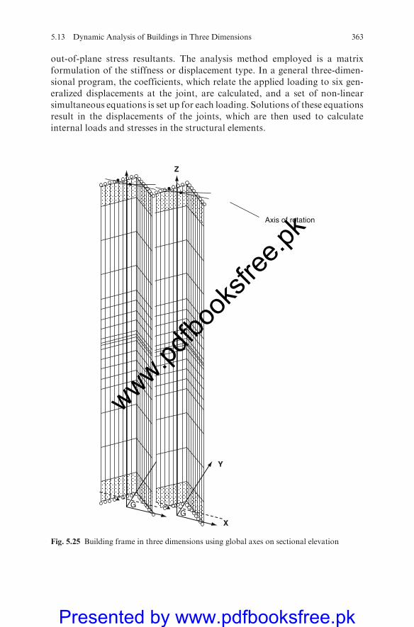
out-of-plane stress resultants. The analysis method employed is a matrix
formulation of the stiffness or displacement type. In a general three-dimen-
sional program, the coefficients, which relate the applied loading to six gen-
eralized displacements at the joint, are calculated, and a set of non-linear
simultaneous equations is set up for each loading. Solutions of these equations
result in the displacements of the joints, which are then used to calculate
internal loads and stresses in the structural elements.
GG
X
Y
Z
Axis of rotation
Fig. 5.25 Building frame in three dimensions using global axes on sectional elevation
5.13 Dynamic Analysis of Buildings in Three Dimensions 363
www.pdfbo
oksfr
ee.pk
Presented by www.pdfbooksfree.pk
Analytical solutions can be obtained for both frame and framed tube struc-tures for high-rise buildings which mostly analysed as 3D structures are com-posed of relatively slender members which can be represented by propertiesalong centroidal axis. Surface systems such as slabs and walls or frames aretreated as an assemblage of finite elements. Many computer packages have thecapability for mixing up different element types and are useful in idealizingproblems of complex shape. External influences such as static, dynamic andblast load temperature and file can be considered in the design of such struc-tures. The reader is advised to refer to Appendix IA for options.
Generation options are available for convenience of inputting largeamounts of data. Many computer programs have plotting capabilities forthe undeformed and deformed shape of the structure for verification of themodel geometry and the structural behaviour of the system. The library ofelements consists of elements from the basic linear element to the mostsophisticated three-dimensional elements. Boundary elements in the form ofspring supports can be incorporated. Loading options include gravity, ther-mal, in addition to the usual nodal loading consisting of either specified forcesor displacements.
Among the dynamic analysis options, two of the most useful ones areeigenvalue analysis and response spectrum analysis. Wind, seismic and blastanalyses by the response spectrum approach require the undamped free vibra-tionmode shapes and frequencies of the system. The response spectrum analysisis obtained by solving the dynamic equilibrium equations by using the modalsuperposition method.
Data preparation involves defining the basic geometric dimensions of thestructure by establishing joints or nodes on the structure.
5.13.2 Finite Element Analysis of Framed Tubular Buildings UnderStatic and Dynamic Load Influences
A tube is a three-dimensional structure and as such responds by bending aboutboth its principal axes and rotation about a vertical axis. In analysing a quarteror half model, it is necessary to restrain the transverse bending and rotation ofthe tube. The kinematic restraints that preclude transverse movement androtation of the model are shown in Fig. 5.26.
5.13.2.1 Lumping Technique
Many structural analyses have used lumping techniques to reduce the size ofanalytical models for computer analysis. The reduction in size was necessi-tated because even with large-capacity computers, there just was no econom-ical way of solving very tall buildings with large numbers of joints. Before thestructural analysis raises its eyebrows in surprise, it is well to bear in mind
364 5 Dynamic Finite Element Analysis of Structures
www.pdfbo
oksfr
ee.pk
Presented by www.pdfbooksfree.pk
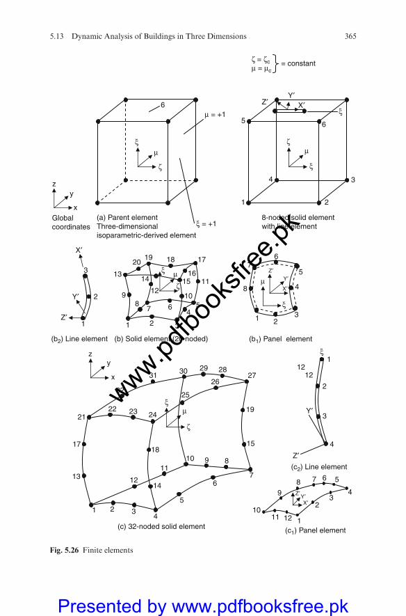
ξ μ
z
ζμ
ξ
6 μ = +1
ξ = +1
6
21
34
5
Z′Y′
X′ξ
ζ = ζcμ = μc
= constant
(a) Parent elementThree-dimensionalisoparametric-derived element
8-noded solid elementwith line element
ξμ
ζ
1 2 3 4
5
6 7
8 9 10
1
12 13 14
15
Z′ 17
18
19 Y′21
22 23 24
25
26
11
2
28 29 27
30 31
32
10
1
23
4
56789
12 11
ξ
3
4
ξ μ
ζ 11
1 2 3
4 5 6 7
8 9 10
12 12
12
13 14 15
16
17 18 19 20
(b) Solid element (20 noded) (b1) Panel element
Z′Y′
X′μ
ξ
1 2 3
4
5
6 7
8
1
2
3
Z′
Y′
X′
zy
x
(b2) Line element
(c1) Panel element(c) 32-noded solid element
(c2) Line element
Globalcoordinates
ζ
x
y
Y′Z′
X′
Fig. 5.26 Finite elements
5.13 Dynamic Analysis of Buildings in Three Dimensions 365
www.pdfbo
oksfr
ee.pk
Presented by www.pdfbooksfree.pk
that many notable buildings have been analysed using lumping techniquesand they have been performing successfully over the years. Therefore,although the speed and capacity of modern mainframe computers are sovast as not to require lumping, introduction of desktop computers withrelatively less capacity has once again required lumped computer modellingtechniques. It is important to realise that as long as the essential features ofthe building are captured in the model, it makes very little difference whethera lumped or a full model is used for the analysis. Of course, there will bedifferences between the results of the two models, especially with regard tothe stress resultants. Under impact and blast load effects, the authors foundvery little difference between the results of lumped and full models as dis-cussed later on.
In this method of analysis, while looking at the entire structure, two floorsare lumped into one floor, the moment of inertia and area of the girder in thelumped model should be twice their values in the prototype model. If n floorsare lumped into one floor, the corresponding properties will be n times theprototype values. To keep the explanation simple, it is useful to introduce thefollowing notations:
Icp ¼ moment of inertia of column in the unlumped model (prototype)Icl ¼ moment of intertia of the column in the lumped modelL = length of girder which is the same in both modelshcp ¼ height of column in the unlumped model (prototype)hcl = height of the column in the lumped modeluf g ¼ element DOF vector_uf g ¼ time derivative of element DOF vector
Kef g ¼ element stiffness/conductivity matrixMef g ¼ element mass matrix
NINT = number of integration pointsNCS =total number of converged substeps
sf g ¼ stress vectoreel�
¼ elastic strain vectorDepl�
¼ plastic strain incrementVoli = volume of integration points
Part C
5.14 Finite Element Modelling of Building Structures – Step by
Step Formulations Incorporating All Previous Sections
5.14.1 Introduction
A step-by-step finite element analysis is developed in which a provision ismade for elasto-plasticity, thermal creep, creep recovery and cracking
366 5 Dynamic Finite Element Analysis of Structures
www.pdfbo
oksfr
ee.pk
Presented by www.pdfbooksfree.pk
under static and dynamic conditions. Various concrete strength theories
described in earlier chapters are included in the finite element analysis.
These give facilities for the comparative study of results necessary for some
sensitive structures. The analysis presented here also includes facilities for
loading and unloading phenomena. Although greater emphasis is given to
the use of isoparametric elements in the text, tables are provided which
will assist in the automatic inclusion of other types of finite elements.
Equations are set up in such a way that they can easily be replaced or
modified to include other case studies. The initial stress or modified
Newton–Raphson method is used for the major solution procedures.
They together with acceleration and convergence procedures can easily
solve non-linear, plasticity and cracking problems. Where dynamic pro-
blems exist, equations of motion are introduced in both linear and non-
linear cases. Expressions for displacements, velocities and accelerations are
then obtained. Direct integration and Wilson-y methods have been used
throughout for the time-dependent solutions of dynamically loaded struc-
tures. The main analysis of this chapter is supported by analyses given in
various tables and appendices. For further study and additional informa-
tion, the references cited in this chapter may be found useful.
5.14.2 Solid Isoparametric Element Representing Concrete
Three-dimensional isoparametric elements are used and the functions relating
to coordinate systems are expressed as follows:
X ¼Pni¼1
Ni x; Z; zð ÞXi ¼ N1x1 þN2x2 þ � � � ¼ Nf gT Xnf g
Y ¼Pni¼1
Ni x; Z; zð ÞYi ¼ N1y1 þN2y2 þ � � � ¼ Nf gT Ynf g
Z ¼Pni¼1
Ni x; Z; zð ÞZi ¼ N1z1 þN2z2 þ � � � ¼ Nf gT Znf g
(5:155)
where Ni x; Z; zð Þ; i ¼ 1 to n, are the interpolation functions in the curvilinear
coordinates x; Z; z and Xi;Yi and Zi are the global X,Y,Z coordinates of mode
i. The interpolation function N is also known as the shape function.The terms Xnf g; Ynf g and Znf g present the nodal coordinates and Nf gT is
dependent on x; Z and z. Reference is made to Fig. 5.26 for important aspects of
the mapping procedures. The most important aspect is to establish a one-to-one
relationship between the derived and the parent element (Fig. 5.26). The neces-
sary condition for a one-to-one relationship is the Jacobian determinant given
in (5.157)
5.14 Finite Element Modelling of Building Structures 367
www.pdfbo
oksfr
ee.pk
Presented by www.pdfbooksfree.pk
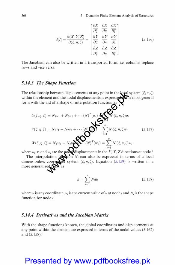
d J½ � ¼ @ X;Y;Zð Þ@ x; Z; zð Þ ¼
@X
@x@X
@Z@X
@z
@Y
@x@Y
@Z@Y
@z
@Z
@x@Z
@Z@Z
@z
266666664
377777775
(5:156)
The Jacobian can also be written in a transported form, i.e. columns replacerows and vice versa.
5.14.3 The Shape Function
The relationship between displacements at any point in the local system x; Z; zð Þwithin the element and the nodal displacements is expressed in the most generalform with the aid of a shape or interpolation function as
U x; Z; zð Þ ¼ N1u1 þN2u2 þ � � � Nð ÞT unð Þ ¼Xni¼1
Ni x; Z; zð Þui
V x; Z; zð Þ ¼ N1v1 þN2v2 þ � � � Nð ÞT vnð Þ ¼Xni¼1
Ni x; Z; zð Þvi
W x; Z; zð Þ ¼ N1w1 þN2w2 þ � � � Nð ÞT wnð Þ ¼Xni¼1
Ni x; Z; zð Þwi
(5:157)
where ui; vi and wi are the nodal displacements in theX, Y, Z directions at node i.The interpolation function Ni can also be expressed in terms of a local
dimensionless coordinate system x; Z; zð Þ. Equation (5.159) is written in amore generalized form as
�u ¼Xni¼1
Ni�ui (5:158)
where �u is any coordinate, �ui is the current value of �u at node i andNi is the shapefunction for node i.
5.14.4 Derivatives and the Jacobian Matrix
With the shape functions known, the global coordinates and displacements atany point within the element are expressed in terms of the nodal values (5.162)and (5.158):
368 5 Dynamic Finite Element Analysis of Structures
www.pdfbo
oksfr
ee.pk
Presented by www.pdfbooksfree.pk
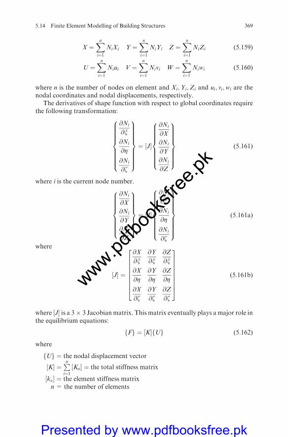
X ¼Xni¼1
NiXi Y ¼Xni¼1
NiYi Z ¼Xni¼1
NiZi (5:159)
U ¼Xni¼1
Niui V ¼Xni¼1
Nivi W ¼Xni¼1
Niwi (5:160)
where n is the number of nodes on element and Xi;Yi;Zi and ui; vi;wi are thenodal coordinates and nodal displacements, respectively.
The derivatives of shape function with respect to global coordinates requirethe following transformation:
@Ni
@x
@Ni
@Z
@Ni
@z
8>>>>>>><>>>>>>>:
9>>>>>>>=>>>>>>>;¼ J½ �
@Ni
@X
@Ni
@Y
@Ni
@Z
8>>>>>><>>>>>>:
9>>>>>>=>>>>>>;
(5:161)
where i is the current node number.
@Ni
@X
@Ni
@Y
@Ni
@Z
8>>>>>><>>>>>>:
9>>>>>>=>>>>>>;¼ J½ �
@Ni
@x@Ni
@Z
@Ni
@z
8>>>>>>><>>>>>>>:
9>>>>>>>=>>>>>>>;
(5:161a)
where
J½ � ¼
@X
@x@Y
@x@Z
@x@X
@Z@Y
@Z@Z
@Z
@X
@z@Y
@z@Z
@z
266666664
377777775
(5:161b)
where J½ � is a 3� 3 Jacobianmatrix. This matrix eventually plays amajor role inthe equilibrium equations:
Ff g ¼ K½ � Uf g (5:162)
where
Uf g ¼ the nodal displacement vector
K½ � ¼Pni¼1
Ke½ � ¼ the total stiffness matrix
ke½ � ¼ the element stiffness matrixn = the number of elements
5.14 Finite Element Modelling of Building Structures 369
www.pdfbo
oksfr
ee.pk
Presented by www.pdfbooksfree.pk
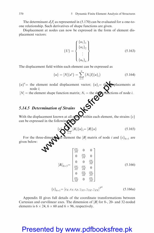
The determinant d J½ � as represented in (5.170) can be evaluated for a one-to-one relationship. Such derivatives of shape functions are given.
Displacement at nodes can now be expressed in the form of element dis-placement vectors:
Uf g ¼
u1f g1u2f g2...
unf gn
8>>>><>>>>:
9>>>>=>>>>;
(5:163)
The displacement field within each element can be expressed as
uf g ¼ N½ � uef g ¼Xni¼1
Ni I½ � uf gi �
(5:164)
uf ge¼ the element nodal displacement vector; uf gi¼ the displacements atnode i;
N½ � ¼ the element shape function matrix; Ni ¼ the shape functions of node i.
5.14.5 Determination of Strains
With the displacement known at all points within each element, the strains ef gcan be expressed in the following form:
ef g ¼Xni¼1
Bi½ � uf gi¼ B½ � uf g (5:165)
For the three-dimensional element the B½ � matrix of node i and ef g6�1 aregiven below:
Bi½ �6�3¼
@Ni
@X 0 0
0 @Ni
@Y 0
0 0 @Ni
@Z
@Ni
@Y@Ni
@X 0
0 @Ni
@Z@Ni
@Y
@Ni
@Z 0 @Ni
@X
266666666664
377777777775
(5:166)
ef g6�1¼ eX; eY; eZ; gXY; gYZ; gZX½ �TH
(5:166a)
Appendix II gives full details of the coordinate transformations betweenCartesian and curvilinear axes. The dimension of B½ � for 8-, 20- and 32-nodedelements is 6� 24, 6� 60 and 6� 96, respectively.
370 5 Dynamic Finite Element Analysis of Structures
www.pdfbo
oksfr
ee.pk
Presented by www.pdfbooksfree.pk

5.14.6 Determination of Stresses
The stresses sf g can be determined within each element from the strains as
sf g ¼ D½ � ef g � e0f g þ s0f gð Þ (5:167)
where s0f g = initial stresses; e0f g = initial strains and D½ � ¼ the materialcompliance matrix.
5.14.7 Load Vectors and Material Stiffness Matrix
Appendix III gives the material matrices D½ � for both concrete and steel. Nowvirtual displacement duef g is applied at the nodes, and the sum of work done,dW, by the stresses and distributed body and surface forces over the elementvolume, vol, and surface, S, is given by
dW¼ duef gTH
h i Zvol
B½ �TH
sf gd vol�ZS
N½ �TH
pf gd S�Zvol
N½ �TH
Gf gd vol
� �(5:168)
where pf g ¼ the surface force per unit surface area; Gf g ¼ the force per unitvolume and TH ¼ transpose of the matrix.
When the external work dW is related to the internal work dU
dW ¼ dU (5:169)The element stiffness matrix K½ �
K½ � ¼Z
volBTH
DBd vol ¼Z þ1�1
Z þ1�1
Z þ1�1
BTH
DB det=dxdZdz (5:170)
The right-hand side of (5.170) is based on the Gaussian integration rule.Equation (5.168) is valid for any virtual displacement duef g, thus it can be
eliminated from both sides of (5.168a). Substituting equations (5.170) and(5.167) into (5.168) one obtains
Pf ge¼Zvol
B½ �TH
D½ � B½ �dV� �
uef g �Zvol
B½ �TH
D½ � e0f gdV
þZvol
B½ �TH
s0f gdV�ZS
N½ �T pf gdS�Zvol
N½ �TH
Gf gdV(5:171)
Table 5.10 gives miscellaneous loads and forces. Equation (5.185) is theforce–displacement relation with stiffness transformation. The terms in(VI.17) are defined as the following:The element stillness matrix
5.14 Finite Element Modelling of Building Structures 371
www.pdfbo
oksfr
ee.pk
Presented by www.pdfbooksfree.pk
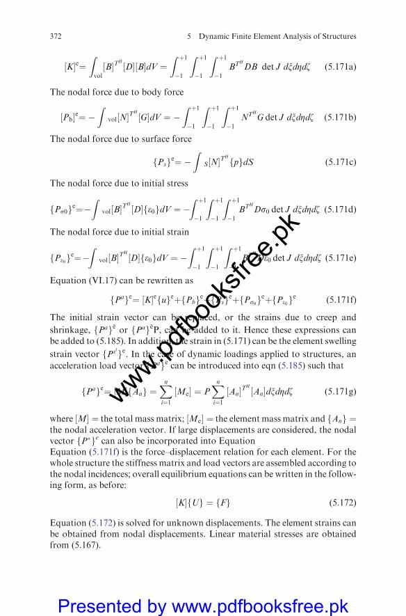
K½ �e¼Zvol
B½ �TH
D½ � B½ �dV ¼Z þ1�1
Z þ1�1
Z þ1�1
BTH
DB det J dxdZdz (5:171a)
The nodal force due to body force
Pb½ �e¼ �Z
vol N½ �TH
G½ �dV ¼ �Z þ1�1
Z þ1�1
Z þ1�1
NTH
G det J dxdZdz (5:171b)
The nodal force due to surface force
Psf ge¼ �Z
S N½ �TH
pf gdS (5:171c)
The nodal force due to initial stress
Ps0f ge¼�Z
vol B½ �TH
D½ � e0f gdV ¼ �Z þ1�1
Z þ1�1
Z þ1�1
BTH
Ds0 det J dxdZdz (5:171d)
The nodal force due to initial strain
Pe0f ge¼�Z
vol B½ �TH
D½ � e0f gdV ¼ �Z þ1�1
Z þ1�1
Z þ1�1
BTH
De0 det J dxdZdz (5:171e)
Equation (VI.17) can be rewritten as
Paf ge¼ K½ �e uf geþ Pbf geþ Psf geþ Ps0f geþ Pe0f ge (5:171f)
The initial strain vector can be replaced, or the strains due to creep and
shrinkage, Paf g�e or Paf g�eP, can be added to it. Hence these expressions canbe added to (5.185). In addition, the strain in (5.171) can be the element swelling
strain vector fPslge. In the case of dynamic loadings applied to structures, an
acceleration load vector Paf ge can be introduced into eqn (5.185) such that
Paf ge¼ M½ � Anf g ¼Xni¼1
Me½ � ¼ PXni¼1
An½ �TH
An½ �dxdZdz (5:171g)
where M½ � ¼ the total mass matrix; Me½ � ¼ the element mass matrix and Anf g ¼the nodal acceleration vector. If large displacements are considered, the nodalvector P�f ge can also be incorporated into EquationEquation (5.171f) is the force–displacement relation for each element. For thewhole structure the stiffness matrix and load vectors are assembled according tothe nodal incidences; overall equilibrium equations can be written in the follow-ing form, as before:
K½ � Uf g ¼ Ff g (5:172)
Equation (5.172) is solved for unknown displacements. The element strains canbe obtained from nodal displacements. Linear material stresses are obtainedfrom (5.167).
372 5 Dynamic Finite Element Analysis of Structures
www.pdfbo
oksfr
ee.pk
Presented by www.pdfbooksfree.pk
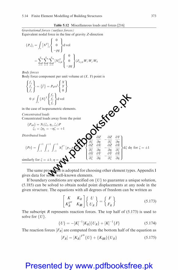
The same procedure is adopted for choosing other element types. Appendix Igives data for some well-known elements.
If boundary conditions are specified on Uf g to guarantee a unique solution,(5.185) can be solved to obtain nodal point displacements at any node in thegiven structure. The equations with all degrees of freedom can be written as
K K �R
KTH
�RK �R�R
" #U
U �R
� �¼
F
F �R
� �(5:173)
The subscript R represents reaction forces. The top half of (5.173) is used tosolve for Uf g.
Uf g ¼ � K½ ��1 K �R½ � U �Rf g þ K½ ��1 Ff g (5:174)
The reaction forces ½FR� are computed from the bottom half of the equation as
F �R½ � ¼ K �R½ �TH
Uf g þ K �R�Rf g U �Rf g (5:175)
Table 5.12 Miscellaneous loads and forces [216]
Gravitational forces (surface forces)Equivalent nodal force in the line of gravity Z-direction
fPsgi ¼Zv
NT�
i
0
0
�pg
8><>:
9>=>;d vol
¼Xni¼1
Xni¼1
Xni¼1
N½ �Ti:jk0
0
�pg
8><>:
9>=>; Jj ji:j:kWi Wj Wk
Body forcesBody force component per unit volume at (X, Y) point is
fxfyfz
8<:
9=; ¼ �f
� ¼ Pbo2
XY0
8<:
9=;
0 6¼Zv
Nf gTfxfyfz
8<:
9=;d vol
in the case of isoparametric elements.
Concentrated loadsConcentrated loads away from the point
Ps0f g ¼ Niðx1; Z1; z1ÞPx1 ¼ xZ1 ¼ �Zz ¼ þ1
Distributed loads
Psf g ¼Z þ1�1
Z þ1�1
Z þ1�1
NT 00
i ½ px; py; pz; �T 00
@Y
@x@Z
@Z� @Z@x
@Y
@Z@Z
@x@X
@Z� @Z@Z
@X
@x@X
@x@Y
@Z� @Y@x
@X
@Z
8>>>>>><>>>>>>:
9>>>>>>=>>>>>>;dx dZ for z ¼ 1
similarly for x ¼ 1; Z ¼ 1:
5.14 Finite Element Modelling of Building Structures 373
www.pdfbo
oksfr
ee.pk
Presented by www.pdfbooksfree.pk
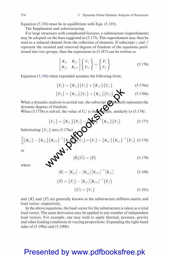
Equation (5.188) must be in equilibrium with Eqn. (5.189).The Supplement and substructuringFor large structures with complicated features, a substructure (superelement)
may be adopted on the lines suggested in (5.173). This superelement may then beused as a reduced element from the collection of elements. If subscripts g and gl
represent the retained and removed degrees of freedom of the equations parti-tioned into two groups, then the expressions in (5.187) can be written as
Kgg Kggl
Kglg Kglgl
" #Ug
Ugl
( )¼
Fg
Fgl
( )(5:176)
Equation (5.190) when expanded assumes the following form:
Fg�
¼ Kgg�
Ug�
þ Kggl�
Ugl�
(5:176a)
Fgl�
¼ Kglg
� Ug�
þ Kglg
� Ugl�
(5:176b)
When a dynamic analysis is carried out, the subscript g (retained) represents thedynamic degrees of freedom.When (5.175b) is solved, the value of Ur
0 is then written, similarly to (5.174)..
Ugl�
¼ Kglg
� Fgl�
� Kglgl� �1
Kglg
� Ug�
(5:177)
Substituting Ugl�
into (5.176a)
Kgg�
� Kglg�
Kglgl� �1
Kglg� h ih i
Ug�
¼ Fg�
� Kggl�
Kggl� �1
Fgl�
(5:178)
or
�K½ � �Uf g ¼ �Ff g (5:179)
where
�K½ � ¼ Kggl�
� Kggl�
Kglgl� �1
Kglg�
(5:180)
�Ff g ¼ Fg�
� Kggl�
Kglgl� �1
Fgl�
�Uf g ¼ Ug�
(5:181)
and �Kf g and �Ff g are generally known as the substructure stiffness matrix andload vector, respectively.
In the above equations, the load vector for the substructure is taken as a totalload vector. The same derivation may be applied to any number of independentload vectors. For example, one may wish to apply thermal, pressure, gravityand other loading conditions in varying proportions. Expanding the right-handsides of (5.190a) and (5.190b)
374 5 Dynamic Finite Element Analysis of Structures
www.pdfbo
oksfr
ee.pk
Presented by www.pdfbooksfree.pk
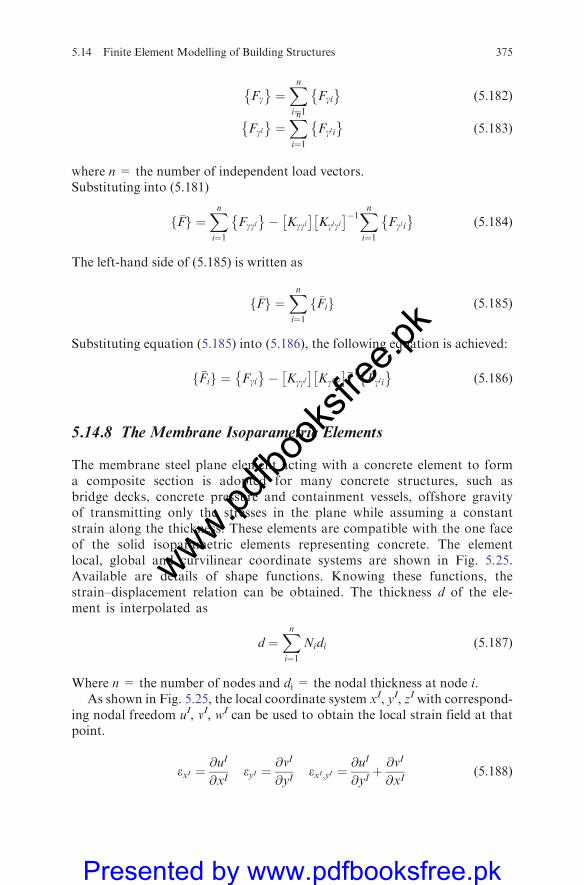
Fg�
¼Xni¼1
Fgi�
(5:182)
Fgl�
¼Xni¼1
Fgl i�
(5:183)
where n = the number of independent load vectors.Substituting into (5.181)
�Ff g ¼Xni¼1
Fggl�
� Kggl�
Kglgl� �1Xn
i¼1Fgl i�
(5:184)
The left-hand side of (5.185) is written as
�Ff g ¼Xni¼1
�Fif g (5:185)
Substituting equation (5.185) into (5.186), the following equation is achieved:
�Fif g ¼ Fgi�
� Kggl�
Kglgl� �1
Fgli
� (5:186)
5.14.8 The Membrane Isoparametric Elements
The membrane steel plane element acting with a concrete element to forma composite section is adopted for many concrete structures, such asbridge decks, concrete pressure and containment vessels, offshore gravityof transmitting only the stresses in the plane while assuming a constantstrain along the thickness. These elements are compatible with the one faceof the solid isoparametric elements representing concrete. The elementlocal, global and curvilinear coordinate systems are shown in Fig. 5.25.Available are details of shape functions. Knowing these functions, thestrain–displacement relation can be obtained. The thickness d of the ele-ment is interpolated as
d ¼Xni¼1
Nidi (5:187)
Where n = the number of nodes and di = the nodal thickness at node i.As shown in Fig. 5.25, the local coordinate system xI, yI, zI with correspond-
ing nodal freedom uI, vI, wI can be used to obtain the local strain field at thatpoint.
exI ¼@uI
@xIeyI ¼
@vI
@yIexI;yI ¼
@uI
@yIþ @v
I
@xI(5:188)
5.14 Finite Element Modelling of Building Structures 375
www.pdfbo
oksfr
ee.pk
Presented by www.pdfbooksfree.pk
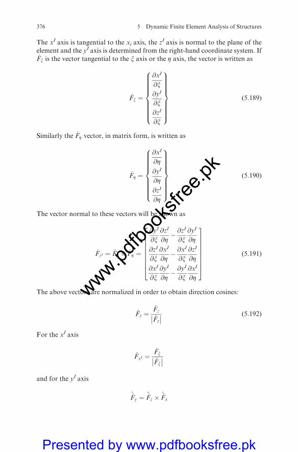
The xI axis is tangential to the xi axis, the zI axis is normal to the plane of the
element and the yI axis is determined from the right-hand coordinate system. IfFx is the vector tangential to the x axis or the Z axis, the vector is written as
Fx ¼
@xI
@x@yI
@x@zI
@x
8>>>>>>><>>>>>>>:
9>>>>>>>=>>>>>>>;
(5:189)
Similarly the FZ vector, in matrix form, is written as
FZ ¼
@xI
@Z@yI
@Z@zI
@Z
8>>>>>>><>>>>>>>:
9>>>>>>>=>>>>>>>;
(5:190)
The vector normal to these vectors will be shown as
FzI ¼ Fx � FZ ¼
@yI
@x@zI
@Z� @z
I
@x@yI
@Z@zI
@x@xI
@Z� @x
I
@x@zI
@Z@xI
@x@yI
@Z� @y
I
@x@xI
@Z
266666664
377777775
(5:191)
The above vectors are normalized in order to obtain direction cosines:
Fz ¼Fz
Fz
�� �� (5:192)
For the xI axis
FxI ¼Fx
Fx�� ��
and for the yI axis
^Fy ¼ ^
Fz � ^Fx
376 5 Dynamic Finite Element Analysis of Structures
www.pdfbo
oksfr
ee.pk
Presented by www.pdfbooksfree.pk
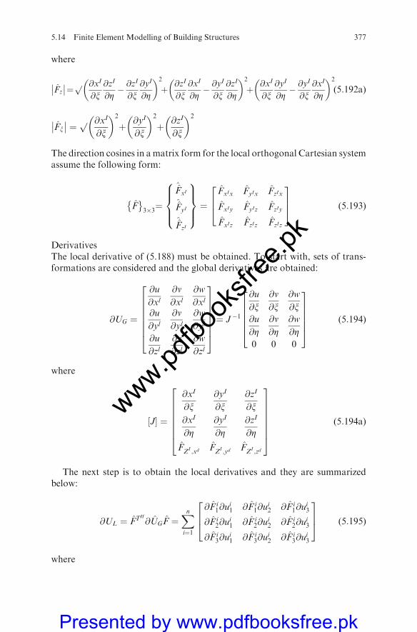
where
Fz
�� ��¼p @xI
@x@zI
@Z� @z
I
@x@yI
@Z
� �2
þ @zI
@x@xI
@Z� @y
I
@x@zI
@Z
� �2
þ @xI
@x@yI
@Z� @y
I
@x@xI
@Z
� �2
(5:192a)
Fx�� �� ¼ p @xI
@x
� �2
þ @yI
@x
� �2
þ @zI
@x
� �2
The direction cosines in amatrix form for the local orthogonal Cartesian systemassume the following form:
F�
3�3¼
^FxI
^FyI
^FzI
8>><>>:
9>>=>>;¼
FxIx FyIx FzIx
FxIy FyIz FzIy
FxIz FzIz FzIz
264
375 (5:193)
DerivativesThe local derivative of (5.188) must be obtained. To start with, sets of trans-formations are considered and the global derivatives are obtained:
@UG ¼
@u
@xl@v
@xl@w
@xl
@u
@yl@v
@yl@w
@yl
@u
@zl@v
@zl@w
@zl
26666664
37777775¼ J �1
@u
@x@v
@x@w
@x@u
@Z@v
@Z@w
@Z0 0 0
266664
377775 (5:194)
where
J½ � ¼
@xI
@x@yI
@x@zI
@x@xI
@Z@yI
@Z@zI
@Z
FZI ;xd FZI ;yd FZI ;zd
26666664
37777775
(5:194a)
The next step is to obtain the local derivatives and they are summarizedbelow:
@UL ¼ FTH
@UGF ¼Xni¼1
@F i1@u
i1 @F i
1@ui2 @F i
1@ui3
@F i2@u
i1 @F i
2@ui2 @F i
2@ui3
@F i3@u
i1 @F i
3@ui2 @F i
3@ui3
264
375 (5:195)
where
5.14 Finite Element Modelling of Building Structures 377
www.pdfbo
oksfr
ee.pk
Presented by www.pdfbooksfree.pk
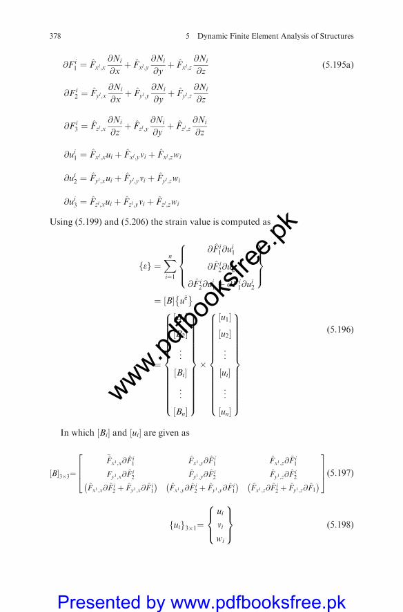
@Fi1 ¼ Fxl;x
@Ni
@xþ Fxl;y
@Ni
@yþ Fxl;z
@Ni
@z(5:195a)
@Fi2 ¼ Fyl;x
@Ni
@xþ Fyl;y
@Ni
@yþ Fyl;z
@Ni
@z
@Fi3 ¼ Fzl;x
@Ni
@zþ Fzl;y
@Ni
@yþ Fzl;z
@Ni
@z
@ui1 ¼ Fxl;xui þ Fxl;yvi þ Fxl;zwi
@ui2 ¼ Fyl;xui þ Fyl;yvi þ Fyl;zwi
@ui3 ¼ Fzl;xui þ Fzl;yvi þ Fzl;zwi
Using (5.199) and (5.206) the strain value is computed as
ef g ¼Xni¼1
@F i1@u
i1
@F i2@u
i2
@F i2@u
i1 þ @F i
1@ui2
8>><>>:
9>>=>>;
¼ B½ � u�e�
¼
B1½ �
B2½ �
..
.
Bi½ �
..
.
Bn½ �
8>>>>>>>>>>>>><>>>>>>>>>>>>>:
9>>>>>>>>>>>>>=>>>>>>>>>>>>>;
�
u1½ �
u2½ �
..
.
ui½ �
..
.
un½ �
8>>>>>>>>>>>>><>>>>>>>>>>>>>:
9>>>>>>>>>>>>>=>>>>>>>>>>>>>;
(5:196)
In which Bi½ � and ui½ � are given as
B½ �3�3¼
�Fx1;x@F
i1 Fx1;y@F
i1 Fx1;z@F
i1
Fy1;x@Fi2 Fy1;y@F
i2 Fy1;z@F
i2
Fx1;x@Fi2 þ Fy1;x@F
i1
�Fx1;y@F
i2 þ Fy1;y@F
i1
�Fx1;z@F
i2 þ Fy1;z@F1
�
2664
3775(5:197)
uif g3�1¼ui
vi
wi
8><>:
9>=>; (5:198)
378 5 Dynamic Finite Element Analysis of Structures
www.pdfbo
oksfr
ee.pk
Presented by www.pdfbooksfree.pk
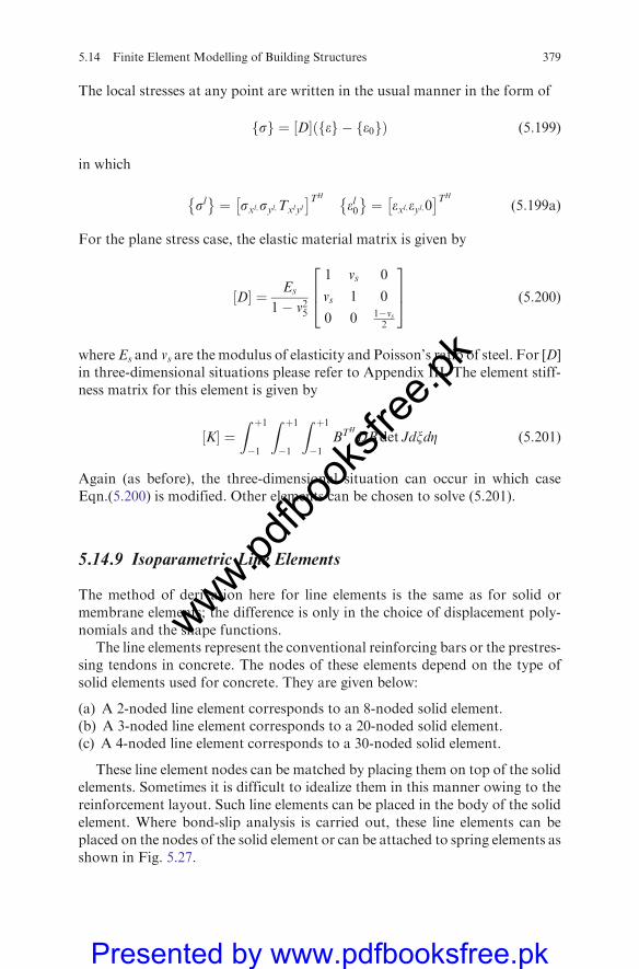
The local stresses at any point are written in the usual manner in the form of
sf g ¼ D½ � ef g � e0f gð Þ (5:199)
in which
sl�
¼ sxl;syl;Txlyl� TH
el0�
¼ exl;eyl;0� TH
(5:199a)
For the plane stress case, the elastic material matrix is given by
D½ � ¼ Es
1� v25
1 vs 0
vs 1 0
0 0 1�vs2
264
375 (5:200)
whereEs and vs are the modulus of elasticity and Poisson’s ratio of steel. For [D]in three-dimensional situations please refer to Appendix III. The element stiff-ness matrix for this element is given by
K½ � ¼Z þ1�1
Z þ1�1
Z þ1�1
BTH
DB det JdxdZ (5:201)
Again (as before), the three-dimensional situation can occur in which caseEqn.(5.200) is modified. Other elements can be chosen to solve (5.201).
5.14.9 Isoparametric Line Elements
The method of derivation here for line elements is the same as for solid ormembrane elements; the difference is only in the choice of displacement poly-nomials and the shape functions.
The line elements represent the conventional reinforcing bars or the prestres-sing tendons in concrete. The nodes of these elements depend on the type ofsolid elements used for concrete. They are given below:
(a) A 2-noded line element corresponds to an 8-noded solid element.(b) A 3-noded line element corresponds to a 20-noded solid element.(c) A 4-noded line element corresponds to a 30-noded solid element.
These line element nodes can be matched by placing them on top of the solidelements. Sometimes it is difficult to idealize them in this manner owing to thereinforcement layout. Such line elements can be placed in the body of the solidelement. Where bond-slip analysis is carried out, these line elements can beplaced on the nodes of the solid element or can be attached to spring elements asshown in Fig. 5.27.
5.14 Finite Element Modelling of Building Structures 379
www.pdfbo
oksfr
ee.pk
Presented by www.pdfbooksfree.pk
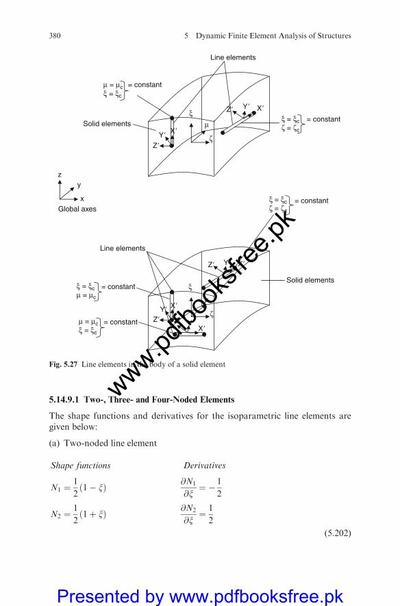
5.14.9.1 Two-, Three- and Four-Noded Elements
The shape functions and derivatives for the isoparametric line elements aregiven below:
(a) Two-noded line element
Shape functions Derivatives
N1 ¼1
21� xð Þ @N1
@x¼ � 1
2
N2 ¼1
21þ xð Þ @N2
@x¼ 1
2
(5:202)
ξμ
ζ
Z� Y� X�
Z�
Y� X�
ξ = ξc = constant ζ = ζc
Line elements
Solid elements
μ = μc = constant ξ = ξc
zy
xGlobal axes
ξ
μ
ζ
Z� Y� X�
Z� Y� X�
ξ = ξc = constant ζ = ζc
μ = μc = constant ξ = ξc
Y�X�
Z�
Line elements
Solid elements ξ = ξc = constant μ = μc
Fig. 5.27 Line elements in the body of a solid element
380 5 Dynamic Finite Element Analysis of Structures
www.pdfbo
oksfr
ee.pk
Presented by www.pdfbooksfree.pk
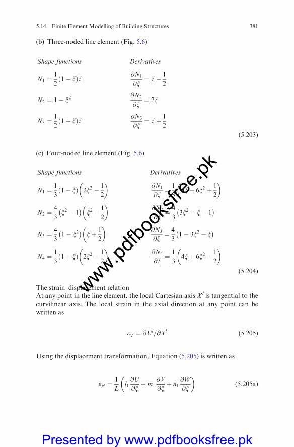
(b) Three-noded line element (Fig. 5.6)
Shape functions Derivatives
N1 ¼1
21� xð Þx @N1
@x¼ x� 1
2
N2 ¼ 1� x2@N2
@x¼ 2x
N3 ¼1
21þ xð Þx @N3
@x¼ xþ 1
2
(5:203)
(c) Four-noded line element (Fig. 5.6)
Shape functions Derivatives
N1 ¼1
31� xð Þ 2x2 � 1
2
� �@N1
@x¼ 1
34x� 6x2 þ 1
2
� �
N2 ¼4
3x2 � 1 �
x2 � 1
2
� �@N2
@x¼ 4
33x2 � x� 1 �
N3 ¼4
31� x2 �
xþ 1
2
� �@N3
@x¼ 4
31� 3x2 � x �
N4 ¼1
31þ xð Þ 2x2 � 1
2
� �@N4
@x¼ 1
34xþ 6x2 � 1
2
� �
(5:204)
The strain–displacement relationAt any point in the line element, the local Cartesian axis Xl is tangential to the
curvilinear axis. The local strain in the axial direction at any point can be
written as
exl ¼ @Ul=@Xl (5:205)
Using the displacement transformation, Equation (5.205) is written as
exl ¼1
Ll1@U
@xþm1
@V
@xþ n1
@W
@x
� �(5:205a)
5.14 Finite Element Modelling of Building Structures 381
www.pdfbo
oksfr
ee.pk
Presented by www.pdfbooksfree.pk
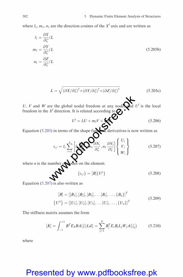
where l1, m1, n1 are the direction cosines of the Xl axis and are written as
l1 ¼@X
@x=L
m1 ¼@Y
@x=L
n1 ¼@Z
@x=L
(5:205b)
L ¼ffiffiffiffiffiffiffiffiffiffiffiffiffiffiffiffiffiffiffiffiffiffiffiffiffiffiffiffiffiffiffiffiffiffiffiffiffiffiffiffiffiffiffiffiffiffiffiffiffiffiffiffiffiffiffiffiffiffiffiffiffiffiffiffiffiffi@X=@xð Þ2þ @Y=@xð Þ2þ @Z=@xð Þ2
q(5:205c)
U, V and W are the global nodal freedom at any node, and Ul is the localfreedom in the Xl direction. It is related according to
Ul ¼ llUþmlVþ nlW (5:206)
Equation (5.205) in terms of the shape function derivatives is now written as
exl ¼ l1Xni¼1
l1@Ni
@x;m1
@Ni
@x; n1
@Ni
@x
� � Ui
Vi
Wi
8><>:
9>=>; (5:207)
where n is the number of nodes on the element.
exlf g ¼ B½ � Uef g (5:208)
Equation (5.207) is also written as
B½ � ¼ B1½ �; B2½ �; B3½ �; . . . Bi½ �; . . . ; Bnf g½ �T
U�e�
¼ U1½ �; U2½ �; U3½ �; . . . Ui½ �; . . . ; Unf g½ �T(5:209)
The stiffness matrix assumes the form
K½ � ¼Z þ1�1
BTESBA xð ÞLdx ¼XNj¼1
BTj EsBjLjWjA xj
�(5:210)
where
382 5 Dynamic Finite Element Analysis of Structures
www.pdfbo
oksfr
ee.pk
Presented by www.pdfbooksfree.pk
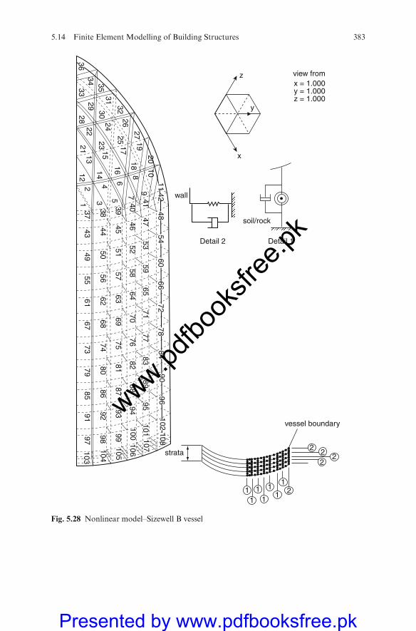
Detail 2 Detail 1
soil/rock
wall
x
y
z
vessel boundary
222
21
111
111
2strata103
104
105
106
107
108102101
10099989791
92
93
94
95
96
85
86
87
88
89
90
79
80
81
82
83
84
73
74
75
76
77
78
67
68
69
70
71
72
61
62
63
64
65
66
55
56
57
58
59
60
49
50
51
52
53
54
43
44
45
46
47
48
37
38
39
40
41
42
12
12
14
16
18
20
1917151321
23
25
27
26242228
30
32
312933
3534
36
4 6
8
10
3 5 7 9
11
view fromx = 1.000y = 1.000z = 1.000
Fig. 5.28 Nonlinear model–Sizewell B vessel
5.14 Finite Element Modelling of Building Structures 383
www.pdfbo
oksfr
ee.pk
Presented by www.pdfbooksfree.pk

A ej �¼Xni¼1
NiAj (5:210a)
where A = the cross-sectional area at node j; n = the number of nodes on the
element; N= the number of integration points and Ni = the shape function at
node i.The strain and stress are calculated as
exlf g ¼ B½ � Uef g sxlf g ¼ ES½ � exlf g (5:211)
where U�ef g is the global nodal displacement of the element.
Fig. 5.29 Finite elementmesh scheme for a concrete
384 5 Dynamic Finite Element Analysis of Structures
www.pdfbo
oksfr
ee.pk
Presented by www.pdfbooksfree.pk

Fig. 5.30 Damage caused by implosion at a level 2.75 times the extreme loads (minimumsafety factor 2.5)
5.14 Finite Element Modelling of Building Structures 385
www.pdfbo
oksfr
ee.pk
Presented by www.pdfbooksfree.pk

Fig. 5.31 Damage caused by implosion at a level 3.5 times the extreme loads (concretecracked/scabbed; steel yielded/plastic)
386 5 Dynamic Finite Element Analysis of Structures
www.pdfbo
oksfr
ee.pk
Presented by www.pdfbooksfree.pk
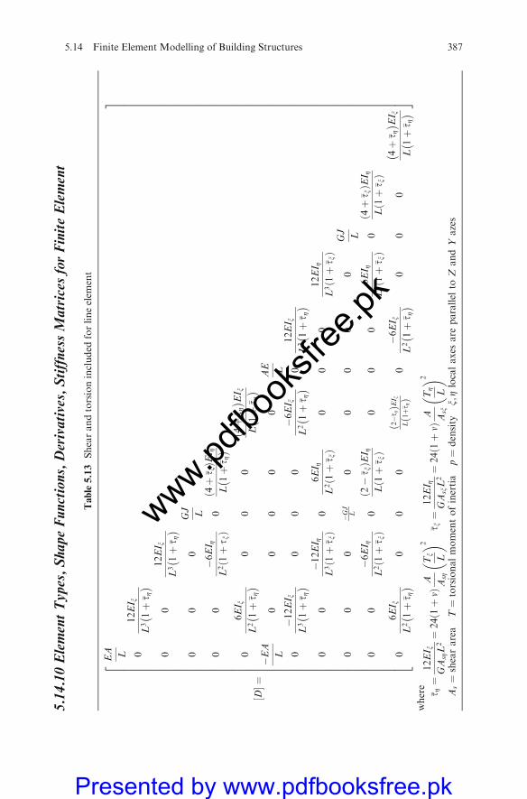
5.14.10ElementTypes,ShapeFunctions,Derivatives,StiffnessMatrices
forFiniteElement
Table5.13
Shearandtorsionincluded
forlineelem
ent
D½�¼
EA L 0
12EI x
L31þ
� t Z
�0
012EI x
L31þ
� t Z
�0
00
GJ L
00
�6EI Z
L21þt x
ðÞ
04þ
� t xð
ÞEI Z
L1þ
� t Z
�0
6EI x
L21þ
�t Z
�0
00
4þ
� t Z
� EIx
L1þ
�t Z
��EA
L0
00
00
AE L
0�12EI x
L31þ
� t Z
�0
00
�6EI x
L21þ
� t Z
�0
12EI x
L31þ
� t Z
�0
0�12EI Z
L31þ
� t xð
Þ0
6EI Z
L21þ
� t xð
Þ0
00
12EI Z
L31þ
� t xð
Þ
00
0�GJ
L0
00
00
GJ L
00
�6EI Z
L21þ
� t xð
Þ0
2�
� t xð
ÞEI Z
L1þ
� t xð
Þ0
00
6EI Z
L21þ
� t xð
Þ0
4þ
� t xð
ÞEI Z
L1þ
� t xð
Þ
06EI x
L21þ
� t Z
�0
00
2�
� t ZðÞE
I x
L1þ
� t ZðÞ
0�6EI x
L21þ
� t Z
�0
00
4þ
� t Z
� EIx
L1þ
� t Z
�
2 6 6 6 6 6 6 6 6 6 6 6 6 6 6 6 6 6 6 6 6 6 6 6 6 6 6 6 6 6 6 6 6 6 6 6 6 6 6 6 6 6 6 6 6 6 4
3 7 7 7 7 7 7 7 7 7 7 7 7 7 7 7 7 7 7 7 7 7 7 7 7 7 7 7 7 7 7 7 7 7 7 7 7 7 7 7 7 7 7 7 7 7 5where
�t Z¼
12EI x
GA
sZL2¼
241þv
ðÞA AsZ
Tx L�� 2
�t x¼
12EI Z
GA
sxL2¼
241þv
ðÞA Asx
TZ L�� 2
As¼
sheararea
T¼
torsionalmomentofinertia
p¼
density
x;Zlocalaxes
are
parallel
toZ
andY
azes
5.14 Finite Element Modelling of Building Structures 387
www.pdfbo
oksfr
ee.pk
Presented by www.pdfbooksfree.pk

5.14.9.2 Line Element in the Body of a Solid Element
The procedure for the strain–displacement and the stiffness matrix is the same
as for the other line elements. The element must lie parallel to one of the
curvilinear axes x; Z; zð Þ of the solid element. The element may be anywhere in
the solid element with maximum curvilinear coordinates x ¼ 1, Z ¼ 1 and
z ¼ 1. The displacement U inside the element is written as (Fig. 5.27)
Table 5.14 Chain rule
@u
@X
@u
@Y
@u
@Z
@v
@X
@v
@Y
@v
@Z
@w
@X
@w
@Y
@w
@Z
26666666666666666666666666666666664
37777777777777777777777777777777775
¼ 1
det J
C11 C12 C13 0 0 0 0 0 0
C21 C22 C23 0 0 0 0 0 0
C31 C32 C33 0 0 0 0 0 0
0 0 0 C11 C12 C13 0 0 0
0 0 0 C21 C22 C23 0 0 0
0 0 0 C31 C32 C33 0 0 0
0 0 0 0 0 0 C11 C12 C13
0 0 0 0 0 0 C21 C22 C23
0 0 0 0 0 0 C31 C32 C33
26666666666666666664
37777777777777777775
@u
@x@u
@Z
@u
@z@v
@x@v
@Z
@v
@z@w
@x@w
@Z
@w
@z
26666666666666666666666666666666666664
37777777777777777777777777777777777775
where
C11 ¼@Y
@x@Z
@x� @Z@Z
@Y
@xC12 ¼
@Z
@x@Y
@z� @Y@x
@Z
@z
C13 ¼@Y
@x@Z
@z� @Z@x
@Y
@zC21 ¼
@Z
@x@X
@z� @X@x
@Z
@z
C22 ¼@X
@x@Z
@z� @Z@x
@X
@zC23 ¼
@Z
@x@X
@Z� @X@x
@Z
@Z
C31 ¼@X
@Z@Y
@z� @Y@Z
@X
@zC32 ¼
@Y
@x@X
@z� @X@x
@Y
@z
C33 ¼@X
@x@Y
@Z� @Y@x
@X
@Z
det J½ � ¼ the determinant of the Jacobian matrix:
388 5 Dynamic Finite Element Analysis of Structures
www.pdfbo
oksfr
ee.pk
Presented by www.pdfbooksfree.pk
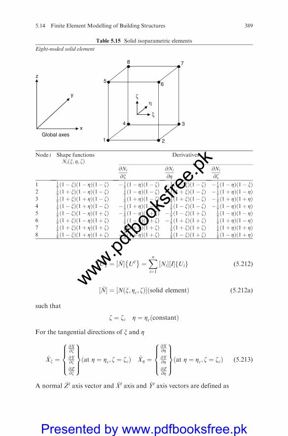
Uf g ¼ �N½ � U�e�
¼Xni¼1
Ni½ � I½ � Uif g (5:212)
�N½ � ¼ N x; Zc; zð Þ½ � solid elementð Þ (5:212a)
such that
z ¼ zc Z ¼ Zc constantð Þ
For the tangential directions of x and Z
Xx ¼
@X@x@Y@x@Z@x
8>><>>:
9>>=>>;
at Z ¼ Zc; z ¼ zcð Þ XZ ¼
@X@Z
@Y@Z
@Z@Z
8>><>>:
9>>=>>;
at Z ¼ Zc; z ¼ zcð Þ (5:213)
A normal Zl axis vector and Xl axis and Yl axis vectors are defined as
Table 5.15 Solid isoparametric elements
Eight-noded solid element
ζη
ξ
6
1 2
34
5
8 7
Global axesx
y
z
Node i Shape functionsNi x; Z; zð Þ
Derivatives
@Ni
@x@Ni
@Z@Ni
@z
1 181� xð Þ 1� Zð Þ 1� zð Þ � 1
81� Zð Þ 1� zð Þ � 1
81� xð Þ 1� zð Þ � 1
81� Zð Þ 1� xð Þ
2 18 1þ xð Þ 1� Zð Þ 1� zð Þ 1
8 1� Zð Þ 1� zð Þ � 18 1þ xð Þ 1� zð Þ � 1
8 1þ Zð Þ 1� Zð Þ3 1
8 1þ xð Þ 1þ Zð Þ 1� zð Þ 18 1þ Zð Þ 1� zð Þ 1
8 1þ xð Þ 1� zð Þ � 18 1þ Zð Þ 1þ Zð Þ
4 181� xð Þ 1þ Zð Þ 1� zð Þ � 1
81þ Zð Þ 1� zð Þ 1
81� xð Þ 1� zð Þ � 1
81� Zð Þ 1þ Zð Þ
5 181� xð Þ 1� Zð Þ 1þ zð Þ � 1
81� Zð Þ 1þ zð Þ � 1
81� xð Þ 1þ zð Þ 1
81� Zð Þ 1� Zð Þ
6 18 1þ xð Þ 1� Zð Þ 1þ zð Þ 1
8 1� Zð Þ 1þ zð Þ � 18 1þ xð Þ 1þ zð Þ 1
8 1þ Zð Þ 1� Zð Þ7 1
81þ xð Þ 1þ Zð Þ 1þ zð Þ 1
81þ Zð Þ 1þ zð Þ 1
81þ xð Þ 1þ zð Þ 1
81þ Zð Þ 1þ Zð Þ
8 181� xð Þ 1þ Zð Þ 1þ zð Þ � 1
81þ Zð Þ 1þ zð Þ 1
81� xð Þ 1þ zð Þ 1
81� Zð Þ 1þ Zð Þ
5.14 Finite Element Modelling of Building Structures 389
www.pdfbo
oksfr
ee.pk
Presented by www.pdfbooksfree.pk
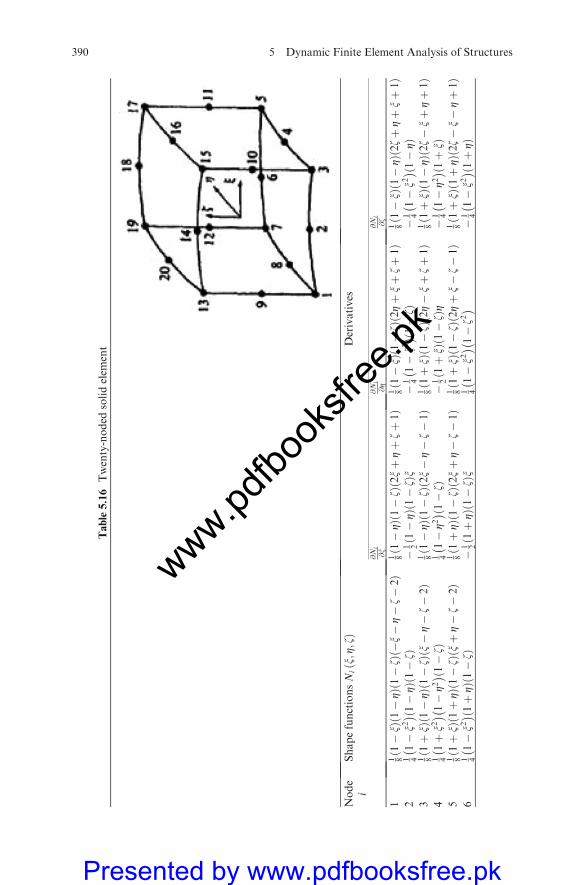
Table5.16
Twenty-noded
solidelem
ent
Node
iShapefunctionsN
iðx;Z;zÞ
Derivatives
@N
i
@x
@N
i
@Z
@N
i
@z
11 81�x
ðÞ1�Z
ðÞ1�z
ðÞ�x�Z�z�2
ðÞ
1 81�Z
ðÞ1�z
ðÞ2xþZþzþ1
ðÞ
1 81�x
ðÞ1�z
ðÞ2Zþxþzþ1
ðÞ
1 81�x
ðÞ1�Z
ðÞ2zþZþxþ1
ðÞ
21 41�x2
� 1�Z
ðÞ1�z
ðÞ
�1 21�Z
ðÞ1�z
ðÞx
�1 41�x2
� 1�z
ðÞ
�1 41�x2
� 1�Z
ðÞ
31 81þx
ðÞ1�Z
ðÞ1�z
ðÞx�Z�z�2
ðÞ
1 81�Z
ðÞ1�z
ðÞ2x�Z�z�1
ðÞ
1 81þx
ðÞ1�z
ðÞ2Z�xþzþ1
ðÞ
1 81þx
ðÞ1�Z
ðÞ2z�xþZþ1
ðÞ
41 41þx2
� 1�Z2
� 1�z
ðÞ
1 41�Z2
� 1�z
ðÞ
�1 21þx
ðÞ1�z
ðÞZ
�1 41�Z2
� 1þx
ðÞ
51 81þx
ðÞð1þZÞð1�zÞ
xþZ�z�2
ðÞ
1 81þZ
ðÞ1�z
ðÞ2xþZ�z�1
ðÞ
1 81þx
ðÞ1�z
ðÞ2Zþx�z�1
ðÞ
1 81þx
ðÞ1þZ
ðÞ2z�x�Zþ1
ðÞ
61 41�x2
� 1þZ
ðÞ1�z
ðÞ
�1 21þZ
ðÞ1�z
ðÞx
1 41�x2
� 1�z2
�
�1 41�x2
� 1þZ
ðÞ
390 5 Dynamic Finite Element Analysis of Structures
www.pdfbo
oksfr
ee.pk
Presented by www.pdfbooksfree.pk
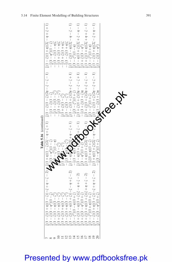
Table5.16
(continued)
71 81�x
ðÞ1þZ
ðÞ1�z
ðÞ�xþZ�z�2
ðÞ
1 81þZ
ðÞ1�z
ðÞ2x�Zþzþ1
ðÞ
1 81�x
ðÞ1�z
ðÞ2Z�x�z�1
ðÞ
1 81�x
ðÞ1þZ
ðÞ2z�Zþxþ1
ðÞ
81 41�x
ðÞ1�Z2
� 1�z
ðÞ
�1 41�Z2
� 1�z
ðÞ
�1 21�x
ðÞ1�z
ðÞ
�1 41�Z2
� 1�x
ðÞ
91 41�x
ðÞ1�Z
ðÞ1�z2
�
�1 41�z2
� 1�Z
ðÞ
�1 41�x
ðÞ1�z2
�
�1 21�x
ðÞ1�Z
ðÞz
10
1 41þx
ðÞ1�Z
ðÞ1�z2
�
1 41�Z
ðÞ1�z2
�
�1 41þx
ðÞ1�z2
�
�1 21þx
ðÞ1�Z
ðÞz
11
1 41þx
ðÞ1þZ
ðÞ1�z2
�
1 41þZ
ðÞ1�z2
�
1 41þx
ðÞ1�z2
�
�1 21þx
ðÞ1þZ
ðÞz
12
1 41�x
ðÞ1þZ
ðÞ1�z2
�
�1 41þZ
ðÞ1�z2
�
1 41�x
ðÞ1�z2
�
�1 21�x
ðÞ1þZ
ðÞz
13
1 81�x
ðÞ1�Z
ðÞ1þz
ðÞ�x�Zþz�2
ðÞ
1 81�Z
ðÞ1þz
ðÞ2xþZ�zþ1
ðÞ
1 81�x
ðÞ1þz
ðÞ2Zþx�zþ1
ðÞ
1 81�x
ðÞ1�Z
ðÞ2z�Z�x�1
ðÞ
14
1 41�x2
� 1�Z
ðÞ1þz
ðÞ
�1 21�Z
ðÞ1þz
ðÞx
�1 41�x2
� 1þz
ðÞ
1 41�x2
� 1�Z
ðÞ
15
1 81þx
ðÞ1�Z
ðÞ1þz
ðÞx�Zþz�2
ðÞ
1 81�Z
ðÞ1þz
ðÞ2x�Zþz�1
ðÞ
1 81þz
ðÞ1þx
ðÞ2Z�x�zþ1
ðÞ
1 81�Z
ðÞ1þx
ðÞ2zþx�Z�1
ðÞ
16
1 41þx
ðÞ1�Z2
� 1þz
ðÞ
1 41�Z2
� 1þx
ðÞ
�1 21þx
ðÞ1þz
ðÞZ
1 41þx
ðÞ1�Z2
�
17
1 81þx
ðÞ1þZ
ðÞ1þz
ðÞxþZþz�2
ðÞ
1 81þZ
ðÞ1þz
ðÞ2xþZþz�1
ðÞ
1 81þx
ðÞ1þz
ðÞ2Zþxþz�1
ðÞ
1 81þx
ðÞ1þZ
ðÞ2zþZþx�1
ðÞ
18
1 41�x2
� 1þZ
ðÞ1þz
ðÞ
�1 2x1þZ
ðÞ1þz
ðÞ
1 41�x2
� 1þz
ðÞ
1 41�x2
� 1þZ
ðÞ
19
1 81�x
ðÞ1þZ
ðÞ1þz
ðÞ�xþZþz�2
ðÞ
1 81þZ
ðÞ1þz
ðÞ2x�Z�z�1
ðÞ
1 81�x
ðÞ1þz
ðÞ2Z�xþz�1
ðÞ
1 81�x
ðÞ1þZ
ðÞ2z�xþZ�1
ðÞ
20
1 41�x
ðÞ1�Z2
� 1þz
ðÞ
�1 41�Z2
� 1þz
ðÞ
�1 21�x
ðÞ1þz
ðÞZ
1 41�x
ðÞ1�Z2
�
5.14 Finite Element Modelling of Building Structures 391
www.pdfbo
oksfr
ee.pk
Presented by www.pdfbooksfree.pk
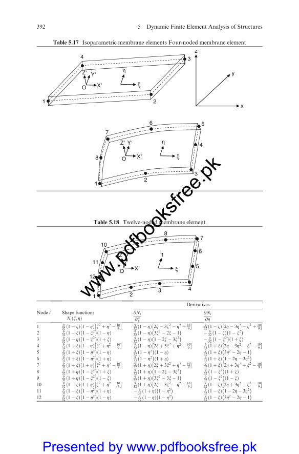
Table 5.17 Isoparametric membrane elements Four-noded membrane element
z
y
x
Z� Y�
X�O
η
ξ
1 2
34
Z� Y�
X�O
η
ξ
12
3
4
56
7
8
Table 5.18 Twelve-noded membrane element
Z� Y�
X�O
η
ξ
1 23 4
5
6
78
910
11
12
Derivatives
Node i Shape functionsNi x; Zð Þ
@Ni
@x@Ni
@Z
1 932 1� xð Þ 1� Zð Þ x2 þ Z2 � 10
9
� 932 1� Zð Þ 2x� 3x2 � Z2 þ 10
9
� 932 1� xð Þ 2Z� 3Z2 � x2 þ 10
9
� 2 9
321� xð Þ 1� x2
�1� Zð Þ 9
321� Zð Þ 3x2 � 2x� 1
�� 9
321� xð Þ 1� x2
�3 9
32 1� Zð Þ 1� x2 �
1þ xð Þ 932 1� Zð Þ 1� 2x� 3x2
�� 9
32 1� x2 �
1þ xð Þ4 9
32 1þ xð Þ 1� Zð Þ x2 þ Z2 � 109
� 932 1� Zð Þ 2xþ 3x2 þ Z2 � 10
9
� 932 1þ xð Þ 2Z� 3Z2 � x2 � 10
9
� 5 9
32 1þ xð Þ 1� Z2 �
1� Zð Þ 932 1� Z2 �
1� Zð Þ 932 1þ xð Þ 3Z2 � 2Z� 1
�6 9
321þ xð Þ 1� Z2
�1þ Zð Þ 9
321� Z2 �
1þ Zð Þ 932
1þ xð Þ 1� 2Z� 3Z2 �
7 932 1þ xð Þ 1þ Zð Þ x2 þ Z2 � 10
9
� 932 1þ Zð Þ 2xþ 3x2 þ Z2 � 19
9
� 932 1þ xð Þ 2Zþ 3Z2 þ x2 � 10
9
� 8 9
32 1þ Zð Þ 1� x2 �
1þ xð Þ 932 1þ Zð Þ 1� 2x� 3x2
�932 1� x2 �
1þ xð Þ9 9
321þ Zð Þ 1� x2
�1� xð Þ 9
321þ Zð Þ 3x2 � 3x� 1
�932
1� x2 �
1� xð Þ10 9
32 1� xð Þ 1þ Zð Þ x2 þ Z2 � 109
� 932 1þ Zð Þ 2x� 3x2 � Z2 þ 10
9
� 932 1� xð Þ 2Zþ 3Z2 � x2 � 10
9
� 11 9
32 1� xð Þ 1� Z2 �
1þ Zð Þ � 932 1þ Zð Þ 1� Z2
�932 1� xð Þ 1� 2Z� 3Z2
�12 9
32 1� xð Þ 1� Z2 �
1� Zð Þ � 932 1� Zð Þ 1� Z2
�932 1� xð Þ 3Z2 � 2Z� 1
�
392 5 Dynamic Finite Element Analysis of Structures
www.pdfbo
oksfr
ee.pk
Presented by www.pdfbooksfree.pk
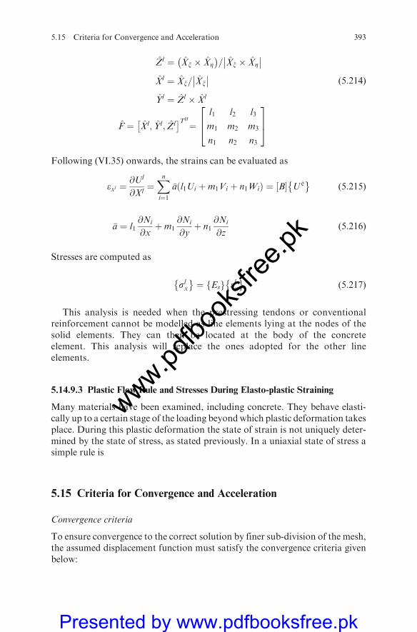
Zl ¼ Xx � XZ �
= Xx � XZ�� ��
Xl ¼ Xx= Xx�� ��
Yl ¼ Zl � Xl
(5:214)
F ¼ Xl; Yl; Zl� TH
¼l1 l2 l3
m1 m2 m3
n1 n2 n3
264
375
Following (VI.35) onwards, the strains can be evaluated as
exl ¼@Ul
@Xl¼Xni¼1
�a l1Ui þm1Vi þ n1Wið Þ ¼ B½ � U�e�
(5:215)
�a ¼ l1@Ni
@xþm1
@Ni
@yþ n1
@Ni
@z(5:216)
Stresses are computed as
slx�
¼ Esf g elx�
(5:217)
This analysis is needed when the prestressing tendons or conventionalreinforcement cannot be modelled as line elements lying at the nodes of thesolid elements. They can then be located at the body of the concreteelement. This analysis will replace the ones adopted for the other lineelements.
5.14.9.3 Plastic Flow Rule and Stresses During Elasto-plastic Straining
Many materials have been examined, including concrete. They behave elasti-cally up to a certain stage of the loading beyondwhich plastic deformation takesplace. During this plastic deformation the state of strain is not uniquely deter-mined by the state of stress, as stated previously. In a uniaxial state of stress asimple rule is
5.15 Criteria for Convergence and Acceleration
Convergence criteria
To ensure convergence to the correct solution by finer sub-division of the mesh,the assumed displacement function must satisfy the convergence criteria givenbelow:
5.15 Criteria for Convergence and Acceleration 393
www.pdfbo
oksfr
ee.pk
Presented by www.pdfbooksfree.pk
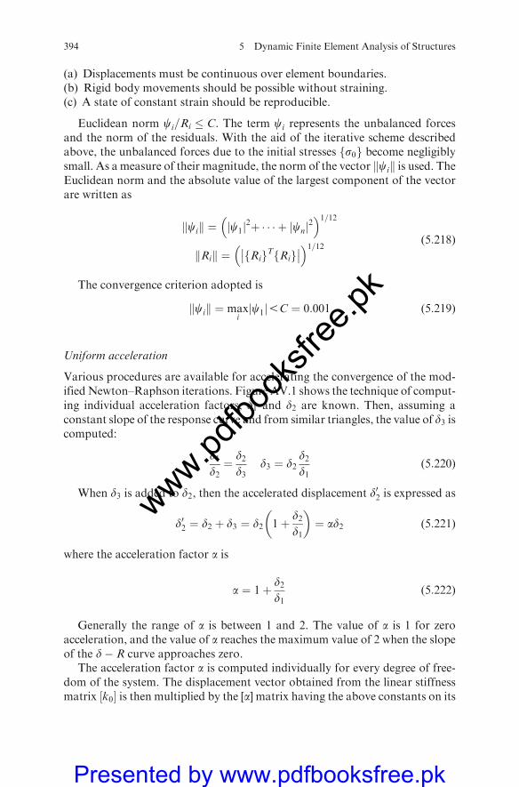
(a) Displacements must be continuous over element boundaries.(b) Rigid body movements should be possible without straining.(c) A state of constant strain should be reproducible.
Euclidean norm ci=Ri � C. The term ci represents the unbalanced forcesand the norm of the residuals. With the aid of the iterative scheme describedabove, the unbalanced forces due to the initial stresses s0f g become negligiblysmall. As a measure of their magnitude, the norm of the vector cik k is used. TheEuclidean norm and the absolute value of the largest component of the vectorare written as
cik k ¼ c1j j2þ � � � þ cnj j
2� �1 12=
Rik k ¼ Rif gT Rif g�� ��� �1 12=
(5:218)
The convergence criterion adopted is
cik k ¼ maxi
c1j j5C ¼ 0:001 (5:219)
Uniform acceleration
Various procedures are available for accelerating the convergence of the mod-ified Newton–Raphson iterations. Figure AV.1 shows the technique of comput-ing individual acceleration factors, d1 and d2 are known. Then, assuming aconstant slope of the response curve and from similar triangles, the value of d3 iscomputed:
d1d2¼ d2
d3d3 ¼ d2
d2d1
(5:220)
When d3 is added to d2, then the accelerated displacement d02 is expressed as
d02 ¼ d2 þ d3 ¼ d2 1þ d2d1
� �¼ ad2 (5:221)
where the acceleration factor a is
a ¼ 1þ d2d1
(5:222)
Generally the range of a is between 1 and 2. The value of a is 1 for zeroacceleration, and the value of a reaches the maximum value of 2 when the slopeof the d� R curve approaches zero.
The acceleration factor a is computed individually for every degree of free-dom of the system. The displacement vector obtained from the linear stiffnessmatrix k0½ � is then multiplied by the [a] matrix having the above constants on its
394 5 Dynamic Finite Element Analysis of Structures
www.pdfbo
oksfr
ee.pk
Presented by www.pdfbooksfree.pk
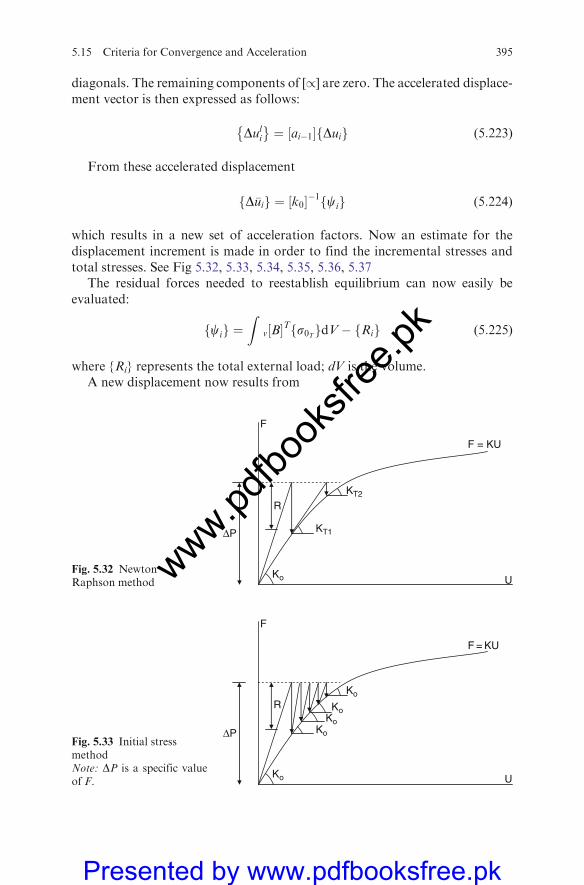
diagonals. The remaining components of [/] are zero. The accelerated displace-ment vector is then expressed as follows:
Duli�
¼ ai�1½ � Duif g (5:223)
From these accelerated displacement
D�uif g ¼ k0½ ��1 cif g (5:224)
which results in a new set of acceleration factors. Now an estimate for thedisplacement increment is made in order to find the incremental stresses andtotal stresses. See Fig 5.32, 5.33, 5.34, 5.35, 5.36, 5.37
The residual forces needed to reestablish equilibrium can now easily beevaluated:
cif g ¼Z
v B½ �T s0Tf gdV� Rif g (5:225)
where {Ri} represents the total external load; dV is the volume.A new displacement now results from
F
F = KU
ΔP
R
KT1
U
KT2
KoFig. 5.32 Newton –Raphson method
F
F = KU
ΔP
R
Ko
U
Ko
Ko
Ko
Ko
Fig. 5.33 Initial stressmethodNote: DP is a specific valueof F.
5.15 Criteria for Convergence and Acceleration 395
www.pdfbo
oksfr
ee.pk
Presented by www.pdfbooksfree.pk
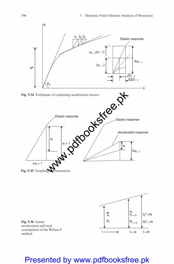
R
Elastic response
ΔP
Ko
δ1 δ2 δ3
Aψi – 1
ψi – 1(A – 1)
(ψi – 1)
ΔUi –1AΔUi – 1
δ
Fig. 5.34 Technique of computing acceleration factors
Elastic response
ψi = 1ψi
Δψi = 1
Aψi – 1
ψi
Elastic response
decelerated response
Fig. 5.35 Graphing representation
t
Rt
δt
t + Δt t + θt
δt + Δt
Rt + Δt Rtn
+ θt
δtn
+ θt
Fig. 5.36 Linearacceleration and loadassumptions of the Wilson-ymethod
396 5 Dynamic Finite Element Analysis of Structures
www.pdfbo
oksfr
ee.pk
Presented by www.pdfbooksfree.pk
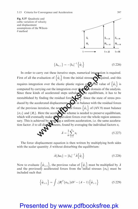
Duiþ1
� ¼ � k0½ ��1 ci
n o(5:226)
In order to carry out these iterative steps, numerical integration is required.
First of all the evaluation of ci
n ofrom the initial stresses is required, and this
requires integration over the elastic–plastic region only. The value of ci
n ois
computed by carrying out the integration over the entire domain of the analysis.Since these kinds of accelerated steps unbalance the equilibrium, it has to be
reestablished by finding the residual forces ci
n o. Since the state of stress pro-
duced by the accelerated displacements is not in balance with the residual forces
of the previous iteration, the new residual forces ci
n oof (AV.9) must balance
sTf g and Rif g. Here the acceleration scheme is needed to preserve equilibrium,which will eventually make the equivalent forces over the whole region unneces-sary. This is achieved by applying a uniform acceleration, i.e. the same accelera-
tion factor �A to all displacements, found by averaging the individual factors ai
�A ¼ 1
n
Xni¼1
ai (5:227)
The force–displacement equation is then written by multiplying both sideswith the scalar quantity �A without disturbing the equilibrium:
�A Duif g ¼ k0½ ��1 �A ci
n o(5:228)
Now to evaluate ciþ1
n o, the previous value of ci
n omust be multiplied by �A
and the previously accelerated forces from the initial stresses s0f g must beincluded such that
ciþ1
n o¼Z
v B½ �T s0Tf gdV� A� 1ð Þ ci�1
n o(5:229)
t
Rt
δt
t + Δt t + θt
δt + Δt
Rt + Δt Rt + θt
δt + θt
Fig. 5.37 Quadratic andcubic variation of velocityand displacementassumptions of the Wilson-y method
5.15 Criteria for Convergence and Acceleration 397
www.pdfbo
oksfr
ee.pk
Presented by www.pdfbooksfree.pk
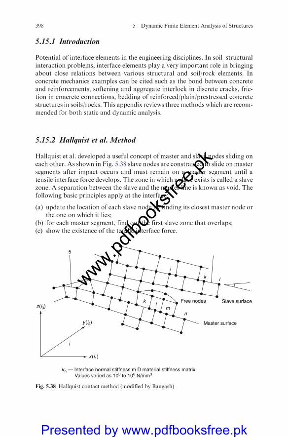
5.15.1 Introduction
Potential of interface elements in the engineering disciplines. In soil–structuralinteraction problems, interface elements play a very important role in bringingabout close relations between various structural and soil/rock elements. Inconcrete mechanics examples can be cited such as the bond between concreteand reinforcements, softening and aggregate interlock in discrete cracks, fric-tion in concrete connections, bedding of reinforced/plain/prestressed concretestructures in soils/rocks. This appendix reviews three methods which are recom-mended for both static and dynamic analysis.
5.15.2 Hallquist et al. Method
Hallquist et al. developed a useful concept of master and slave nodes sliding oneach other. As shown in Fig. 5.38 slave nodes are constrained to slide on mastersegments after impact occurs and must remain on a master segment until atensile interface force develops. The zone in which a slave exists is called a slavezone. A separation between the slave and the master line is known as void. Thefollowing basic principles apply at the interface:
(a) update the location of each slave node by finding its closest master node orthe one on which it lies;
(b) for each master segment, find out the first slave zone that overlaps;(c) show the existence of the tensile interface force.
Free nodes Slave surface
Master surface
kz(i3)
y(i2)
kn — Interface normal stiffness m D material stiffness matrix Values varied as 103 to 106 N/mm3
i
x(i1)
k l
i
lm
n
5
Fig. 5.38 Hallquist contact method (modified by Bangash)
398 5 Dynamic Finite Element Analysis of Structures
www.pdfbo
oksfr
ee.pk
Presented by www.pdfbooksfree.pk
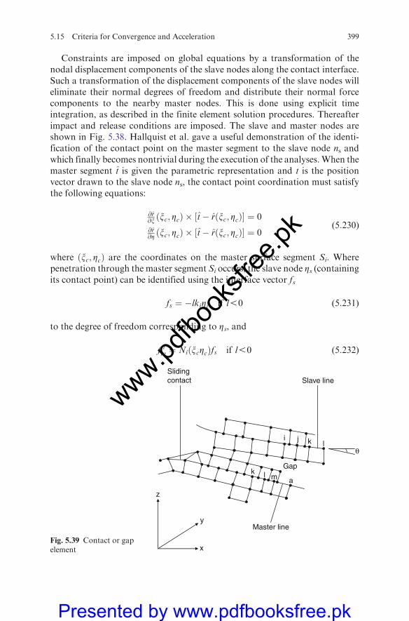
Constraints are imposed on global equations by a transformation of thenodal displacement components of the slave nodes along the contact interface.Such a transformation of the displacement components of the slave nodes willeliminate their normal degrees of freedom and distribute their normal forcecomponents to the nearby master nodes. This is done using explicit timeintegration, as described in the finite element solution procedures. Thereafterimpact and release conditions are imposed. The slave and master nodes areshown in Fig. 5.38. Hallquist et al. gave a useful demonstration of the identi-fication of the contact point on the master segment to the slave node ns andwhich finally becomes nontrivial during the execution of the analyses. When themaster segment t is given the parametric representation and t is the positionvector drawn to the slave node ns, the contact point coordination must satisfythe following equations:
@r@x xc; Zcð Þ � t� r xc; Zcð Þ½ � ¼ 0
@r@Z xc; Zcð Þ � t� r xc; Zcð Þ½ � ¼ 0
(5:230)
where xc; Zcð Þ are the coordinates on the master surface segment Si. Wherepenetration through the master segment Si occurs, the slave node Zs (containingits contact point) can be identified using the interface vector fs
fs ¼ �lkiZi if l50 (5:231)
to the degree of freedom corresponding to Zs, and
f im ¼ Ni xcZcð Þfs if l50 (5:232)
z
y
x
Gap
Slave line
Master line
k l m a
k li
Slidingcontact
θ
j
Fig. 5.39 Contact or gapelement
5.15 Criteria for Convergence and Acceleration 399
www.pdfbo
oksfr
ee.pk
Presented by www.pdfbooksfree.pk
where
l ¼ ni � t� r xc; Zcð Þ½ �50 (5:233)
A unit normal
ni ¼ ni xc; Zcð Þ; ti ¼ niXnj¼1
Nj F1ð Þ jðtÞ (5:234)
ki ¼ fsiKiA2i A2
i Vi
�(5:235)
where
F1ð Þ jðtÞ ¼ impact at the jth nodeK ¼ stiffness factorKi;Vi;Ai ¼ bulk modulus, volume and face area, respectivelyfsi ¼ scale factor normally defaulted to 0.10Ni ¼ 1
41þ xxið Þ 1þ ZZið Þ for a four-node linear surface
Bangash extended this useful analysis for other shape functions, such as Ni
for 8-noded and 12-noded elements. On the basis of this theory and owing to thenon-availability of the original computer source, a new sub-program CON-TACTwas written in association with the program ISOPAR. The sub-programCONTACT is in three dimensions.
FN
� ¼ Kgg�
iUg�
i¼P
k½ �P
Di;Dj; . . .�
¼ Fi;j...
� þ mFn . . . Di . . .�
Dsl ¼ distance of sliding
¼ Dj � Di
�� m Fnj j
Kggj jm ¼ friction
FSN
� � m FN
� no sliding
� m FN
� sliding
¼ 0 contact broken
y ¼ cos�1 Xg or sin�1 Y
g
Bibliography
Ali, H. M. and Abdel-Ghaffar, A. M. Modelling of rubber and lead passive-control bearingsfor seismic analysis. J. Struct. Eng. 1995; 121(7):1134–1144.
Bangash M.Y.H. Shock Impact and Explosion, Springer/Verlag 2009.Bangash M.Y.H. and Bangash T. Shock Impact and Explosion Resistant. swedep Springer
Verlag.
400 5 Dynamic Finite Element Analysis of Structures
www.pdfbo
oksfr
ee.pk
Presented by www.pdfbooksfree.pk

Barbat, A. H. and Bozzo, L. M. Seismic analysis of base isolated buildings. Arch. Comput.Methods Eng. 1997; 4(2):153–192.
Barbat, A. H. and Miquel-Canet, J. Estructuras Sometidas a Acciones Sismicas. CentroInternacional de Metodos Numericos en Ingenieria CIMNE, Barcelona 1994.
Barbat, A., Oller, S., Onate, E., and Hanganu, A. Viscous damage model for Timoshenkobeam structures. Int. J. Solids Struct. 1997; 34(30):3953–3976.
Bathe, K. J. Finite Element Procedures. Prentice-Hall, NJ, 1996.Bhatti, M. A., Pister,K. S., and Polak, E. Optimization of control devices in base isolation
system for aseismic design. Structural Control (Leipholz, H. H. E., ed.). North-HollandPublishing Co., Amsterdam, The Netherlands, 1979; pp. 127–138.
Chopra and Chandrasekaren. Absorber system for earthquake excitation. Proc. 4th WorldConf. Earthquake Eng., Chile, 1969; Vol. II, pp. 139–148.
CSO Volume 7 (User), Book 1: Fortuoi Write Ups, Computing Services Office, University ofIllinois, Urbana, IL, 1974.
Den Hartog, J. P. Mechanical Vibrations (4th edn.). McGraw-Hill, New York, 1956.Dong, R. G. Vibration-absorber effect under seismic excitation. J. Struct. Div. (ASCE) 1976;
102:2021–2031.Feng,M. Q. Application of hybrid sliding isolation system to buildings. J. Engrg.Mech. 1993;
119(10):2090–2108.Feng, M. Q., Shinozuka, M., and Fujii, S. Friction-controllable sliding isolation system.
J. Engrg. Mech. (ASCE) 1993; 119(9):1845–1864.Fuller, K. N. G., Gough, J., Pound, T. J., and Ahmadi, H. R. High damping natural rubber
seismic isolators. J. Struct. Control 1997; 4(2):19–40.Fur, L. S., Yang, H. T. Y., and Ankireddi,S. Vibration control of tall buildings under seismic
and wind loads. J. Struct. Engrg. (ASCE) 1994; 122(8):948–957.Gadala, M. S. Alternative methods for the solution of hyperelastic problems with incompres-
sibility. Comp. Struct. 1992; 42(1):1–10.Govindjee, S. and Simo, J. C. ‘Mullins’ effect and the strain amplitude dependence of the
storage modulus. Int. J. Solids Struct. 1992; 2(14/15):1737–1751.Gupta,Y. P. andChandrasekaren, A. R. Absorber system for earthquake excitation.Proc. 4th
World Conf. Earthquake Eng., Santiago, Chile II, 1969; pp. 139–148.Hanganu, D. A. Analisis no lineal estatico y dinamico de estructuras de hormigon armado
mediante modelos de dano. Ph.D. Thesis, Escuela Tecnica Superior de Ingenieros deCaminos Canales y Puertos de Barcelona, Universidad Politecnica de Cataluna, 1997.
Heinsbroek, A. G. T. J. and Tijsseling, A. S. Seismic Isolation and Response Control forNuclear and Non-Nuclear Structures. Structural Mechanics in Reactor Technology,SMiRT11, Tokyo, Japan 1991.
Hermann, L. R., Hamidi, R., Shafigh-Nobari, F., and Lim, C. K. Nonlinear behaviour ofelastromeric bearings, I: Theory. J. Eng. Mech. 1988; 114(11):1811–1830
Hermann, L. R., Hamidi, R., Shafigh-Nobari, F., and Ramaswamy, A. Nonlinear behaviourof elastomeric bearings. II:FE analysis and verification. J. Eng. Mech. 1998; 114(11):1831–1853.
Housner, G.W. Intensity of Earthquake ground shaking near the causative fault. Proc. 3rdworld conference on Earthquake Engineering, NewZealand, Vol 1, pp. III. Jan. 1965,94–115.
Hwang, J. S. and Ku, S. W. Analytical modelling of high damping rubber bearings. J. Struct.Eng. 1997; 123(8):1029–1036.
Jagadish, K. S., Pradas, B. K. R., and Rao, P. V. The inelastic vibration absorber subjected toearthquake ground motions. Eng. Struct. Dyn. 1979; 7:317–326.
Jalihal, P., Utku, S., and Wada, B. K. Active base isolation in buildings subjected to earth-quake excitation. Proc. 1994 Int. Mech. Eng. Cong. Exposition, Chicago, Illinois, 1994;DSC-Vol. 55-1, pp. 381–388.
Bibliography 401
www.pdfbo
oksfr
ee.pk
Presented by www.pdfbooksfree.pk
Jangid, R. S. Seismic response of sliding structures to bi-directional earthquake excitation.Earthquake Eng. Struct. Dyn. 1996; 25:1301–1306.
Jangid, R. S. Response of pure-friction sliding structures to bi-directional harmonic groundmotion. Eng. Struct. 1997; 19:97–104.
Kaliske, M., Gebbeken, N., and Rothert, H. A generalized approach to inelastic behaviour atfinite srains-Application to polymeric material. Proc. 5th Int. Conf. Comput. Plasticity,Centro Internacional de Metodos Numericos en Ingenieria CIMNE, Barcelona, 1997;pp. 937–944.
Kaynia, A. M., Veneziano, D., and Biggs, J. M. Seismic effectiveness of tuned mass dampers.J. Struct. Div. (ASCE) 1981; 107:1465–1484.
Kelly, J. M. Control devices for earthquake-resistant structural design. Structural Control(Leipholz, H. H. E., ed.). North-Holland Publishing Co., Amsterdam, The Netherlands,1979; pp. 391–413.
Kelly, J. M. Dynamic and Failure Characteristics of Bridgestone Isolation Bearings. Earth-quake Engineering Research Center, College of Engineering, University of California,Berkley, 1991.
Kelly, J. M. Final Report on the International Workshop on the Use of Rubber-Based Bearingfor the Earthquake Protection of Buildings. Earthquake Engineering Research Center,College of Engineering, University of California, Berkley 1995.
Kelly, J. M., Leitmann, G., and Soldatos, A. G. Robust control of base-isolated structuresunder earthquake excitation. J. Optim. Theory Appl. 1987; 53(2):159–180.
Koh, C. G. and Kelly, J. M. Viscoelastic stability model for elastometric isolation bearings.J. Struct. Eng. 1989; 115(2):285–302.
Krieg, R. D. and Krieg, D. N. Accuracy of numerical solution methods for the elastic,perfectly plastic model. Pres. Ves. Technol. 1977; 99:510–515.
Lead hula-hoops stabilize antenna. Eng. News-Record July 22 1976; 10.Li, Z., Rossow, E. C., and Shah, S. P. Sinusoidal forced vibration of sliding masonry system.
Struct. Eng. (ASCE) 1989; 115:1741–1755.Liaw, T. C., TIan,Q. L., and Cheung, Y. K. Structures on sliding base subjected to horizontal
and vertical motions. Struct Eng. (ASCE) 1988; 114:2119–2129.Lin, B. C. and Tadjbakhsh, I. G. Effect of vertical motion on friction driven systems. Earth-
quake Eng. Struct. Dyn. 1986; 14:609–622.Loh,C. H. and Chao, C. H. Effectiveness of active tuned mass damper and seismic
isolation on vibration control of multi-storey building. J. Sound Vibration 1996;193(4):773–792.
Lu, L. Y. and Yang, Y. B. Dynamic response of equipment in structures with sliding support.Earthquake Eng. Struct. Dyn. 1997; 26:61–77.
Luco, J. E., Wong, H. L., andMita, A. Active control of the seismic response of structures bycombined use of base isolation and absorbing boundaries. Earthquake Eng. Struct. Dyn.1992; 21(6):525–541.
Luft, R. W. Optimal tuned mass dampers for buildings. J. Struct. Div. (ASCE) 1979; 105:2766–2772.
McNamara, R. J. Tuned mass dampers for buildings. J. Struct. Div. (ASCE) 1977; 103:1785–1798.
Meirovitch, L. Dynamics and Control Of Structures. Wiley-Interscience, New York, 1990.Meirovitch, L. Principles and Techniques of Vibrations. Prentice-Hall, Inc., Englewood Cliffs,
NJ, 1997.Miyama, T. Seismic response of multi-storey frames equipped with energy absorbing storey on
its top.Proc. 10thWorld Conf. Eng., Madrid, Spain, 19–24 July 1992; Vol. 7, pp. 4201–4206.Mokha, A., Constantinou, M. C., and Reinhorn, A. M. Verification of friction model of
Teflon bearings under triaxial load. Struct. Eng. (ASCE) 1993; 119:240–261.
402 5 Dynamic Finite Element Analysis of Structures
www.pdfbo
oksfr
ee.pk
Presented by www.pdfbooksfree.pk

Molinares, N. and Barbat A. H. Edificios con aislamiento de base no lineal. Monografias deIngenieria Sismica 5, Centre Internacional deMetodos Numericos en Ingenieria, CIMNE,Barcelona 1994.
Moore, J.K.Anonlinear finite element analysis of elastomeric bearings, Ph.D.Thesis, Departmentof Civil Engineering, University of California at Davis, 1982.
Morman, K. The generalized strain measure with application to non-homogeneous deforma-tions in rubber-like solids. J. Appl. Mech. 1986; 53:726–728.
Mostaghel, N., Hejazi, M., and Tanbakuchi, J. Response of sliding structure to harmonicsupport motion. Earthquake Eng. Struct. Dyn. 1983; 11:355–366.
Mostaghel, N. and Khodaverdian, M. Dynamics of resilient-friction base isolator (R-FBI).Earthquake Eng. Struct. Dyn. 1987; 15:379–390.
Mostaghel, N. and Tanbakuchi, J. Response of sliding structures to earthquake supportmotion. Earthquake Eng. Struct. Dyn. 1983; 11:729–748.
Nagarajaiah, S., Li, C., Reinhorn, A., and Constantinou, M. 3D-BASIS-TABS: version 2.0computer program for nonlinear dynamic analysis of three dimensional base isolatedstructures.Technical Report NCEER-94-0018, National Centre for Earthquake EngineeringResearch, University, Buffalo, 1994.
Nagarajaiah, S., Reinhorn, A. M., and Constantinou, M. C. Nonlinear dynamic analysis of3-D-Base-isolated structures. J. Struct. Eng. 1991; 117(7):2035–2054.
Newmark, N.N. Amethod of computation for structural dynamics. J. Eng. Mech, Div. Asck,Vol 85, Nov. EM3, July 1959, pp. 67–94.
Newmark, N.M. and Rosen Blueth E., Fundamentals of earthquake engineering, PrenticeHall, Inc. Englewood chipps, N.I 1971., pp. 162–163.
Odgen, R. W. Nonlinear Elastic Deformations. Ellis Horwood, Chichester, England, 1984.Oller, S.Modelizacion Numerica de Materiales Friccionales. Monografia 3, Centro Internacional
de Metodos Numericos en Ingenieria CIMNE, Barcelona, 1991.Oller, S., Onate, E., Miquel, J., and Botello, S. A plastic damage constitutive model for
composite materials. Int. J. Solids Struct. 1996; 33(17):2501–2518.Onate, E. Calculo de estructuras por el Metodo de los Elementos Finitos. Centro Internacional
de Metodos Numericos en Ingenieria CIMNE, Barcelona, 1992.Ormondroyd, J. and Den Hartog, J. P. The theory of the dynamic vibration absorber. Trans.
(ASME) 1928; APM-50-7:9–22.Pu, J. P. and Kelly,M. Active control and seismic isolation. J. Eng. Mech. ASCE 1991;
117(10):2221–2236.Qumaroddin, M., Rasheeduzzafar, Arya,A. S., and Chandra, B. Seismic response of masonry
buildings with sliding substructure. Struct. Eng. ASCE 1986; 112:2001–2011.Reinhorn, A. M., Soong, T. T., and Wen, C. Y. Base isolated structures with active control.
Recent Advances in Design, Analysis, Testing andQualificationMethods. ASMEPVP 1987;127:413–419.
Rofooei, F. R. and Tadjbakksh, I. G. Optimal control of structures with acceleration,velocity, and displacement feedback. J. Engrg. Mech. ASCE 1993; 119(10): 1993–2010.
Salomon, O. Estructuras con sistema de aislamiento sismico. Analisis por Elementos Finitos.Master’s Thesis, Escuela Tecnica Superior de Ingenieros de Caminos Canales y Puertos deBarcelona, Universidad Politecnica de Cataluna, 1995.
Salomon, O., Oller, S. and Barbat, A. Modelling of laminated elastomeric passive-controlbearing for seismic analysis. Fourth World Cong. Comput. Mech., Buenos Aires, Argentina,1998.
Simo, J. C. A framework for finite strain elastoplasticity based on maximum plastic dissipa-tion and the multiplicative decomposition: Part 2 computational aspects. Comp. MethodsAppl. Mech. Eng. 1988; 68:1–31.
Simo, J. C. Algorithms for static and dynamic multiplicative plasticity that preserve theclassical return mapping schemes of the infinitesimal theory. Comp. Methods Appl.Mech. Eng. 1992; 99:61–112.
Bibliography 403
www.pdfbo
oksfr
ee.pk
Presented by www.pdfbooksfree.pk
Simo, J. C. and Taylor, R. L. Quasi-incompressible finite elasticity in principal stretches.Continuum basis and numerical algorithms. Comp. Methods Appl. Mech. Eng. 1991;85:273–310.
Skinner, R. I., Robinson,W. H., andMcVerry, G.An Introduction to Seismic Isolation. Wiley,Chichester, 1993.
Sladek, J. R. andKlingner, R. E. Effect of tuned-mass dampers on seismic response. J. Struct.Div. (ASCE) 1983; 109:2004–2009.
Sner, M. and Utku, S. Active-passive base isolation system for seismic response controlledstructures. Proc. 36th AIAA/ASME/ASCE/AHS/ASC Struct. Struct. Dyn. Mat. Conf.AIAA/ASME Adaptive Struct. Forum Part 4 (of 5), New Orleans, Louisiana, 1995;pp. 2350–2359.
Sussman, T. and Bathe, K. A finite element formulation for nonlinear incompressible elasticand inelastic analysis. Comp. Struct. 1987; 26(1/2):357–409.
Tower’s cables handle wind, water tank damps it. Eng. News-Record Dec. 9 1971; 23.Tuned mass dampers steady sway of skyscrapers in wind. Eng. News-Record Aug. 18 1977;
28–29.Villaverde, R. Earthquake response of systems with nonproportional damping by the con-
ventional response spectrum method. Proc. 7th World Conf. Earthquake Eng., Istambul,Turkey 1980; Vol. 5, pp. 467–474.
Villaverde, R. Reduction in seismic response with heavily-damped vibration absorbers.Earth-quake Eng. Struct. Dyn. 1985; 13:33–42.
Villaverde, R. Seismic control of structures wih damped resonant appendages. Proc. 1stWorld Conf. Struct. Control, Los Angeles, California, USA, 1994; WP4-113–WP4-119.
Villaverde, R. and Koyama, L. A. Damped resonant appendages to increase inherent damingin buildings. Earthquake Eng. Struct. 1993; 22:491–507.
Villaverde, R. and Martin, S. C. Passive seismic control of cable-stayed bridges with dampedresonant appendages. Earthquake Eng. 1995; 24:233–246.
Villaverde, R. and Newmark, N. M. Seismic response of light attachments to buildings. SRSNo. 469, University of Illinois, Urbana, IL, 1980.
Watari, A. and Sano, I. Optimum tuning of the dynamic damper to control response ofstructures to earthquake ground. Sixth World Conf. Earthquake Eng., New Delhi, India,1977; Vol. 3, pp. 157–161.
Westermo, B. and Udwadia, F. Periodic response of a sliding oscillator system to harmonicexcitation. Earthquake Eng. Struct. Dyn. 1983; 11:135–146.
Wirsching, P. H. and Campbell, G. W. Minimal structural response under random excitationusing vibration absorber. Earthquake Dyn. 1974; 2:303–312.
Wirsching, P. H. and Yao, J. T. P. Safety design concepts for seismic structures. Comput.Struct. 1973; 3:809–826.
Yang, J. N., Danielians, A., and Liu, S. C. Aseismic hybrid control systems for buildingstructures. J. Engrg. Mech. (ASCE) 1991; 117(4): 836–853.
Yang, J. N., Danielians, A., and Liu, S. C. Aseismic hybrid control of nonlinear and hystereticstructures, I. J. Engrg. Mech. (ASCE) 1992a; 118(7):1423–1440.
Yang, J. N., Danielians, A., and Liu,S. C. Aseismic hybrid control of nonlinear and hystereticstructures, I. J. Engrg. Mech. (ASCE) 1992b; 118(7):1441–1456.
Yang, Y. B., Lee, T. Y., and Tsai, I. C. Response of multi-degree-of-freedom structures withsliding supports. Earthquake Eng. Struct. Dyn. 1990; 19:739–752.
Younis,C. J. and Tadjbakhsh, I. G. Response of sliding structure to base excitation. Eng.Mech. (ASCE) 1984; 110:417–432.
404 5 Dynamic Finite Element Analysis of Structures
www.pdfbo
oksfr
ee.pk
Presented by www.pdfbooksfree.pk
Chapter 6
Geotechnical Earthquake Engineering
and Soil–Structure Interaction
6.1 General Introduction
In earthquake engineering, geotechnics plays a prime part. To begin with the
knowledge of soil mechanics for areas related to seismic history is essential. The
understanding of basic dynamics as given in earlier chapters is a must. It is vital
that shaking of the soft ground in earthquakesmust have historical records. The
rupture of fault as a cause of earthquake must be treated as a part of seismo-logical knowledge. Earthquake waves are as P- and S-waves, love wave and
Rayleigh wave. The engineer must know the response of elastic ground to
surface excitation, seismic wave energy and the wave transmission and reflec-
tion at interface. To assess the behaviour of particularly heavy structures in
earthquakes, the soil must be related to the overall performance of structures.
The following are clearly essential to perform the soil–structure interaction.
(a) The intensity of earthquake motion and motion records(b) Time history of the ground motion and power of acceleration–time history(c) Earthquake magnitude and acceleration and duration(d) Effects of local soil conditions on maximum acceleration(e) Significance of outcrop motion(f) Response of multilayered ground and amplification of motion of particu-
larly alluvium surface and at the top hill(g) Direction of seismic criteria force(h) Damping ratio in soils(i) Direction of seismic inertia force and wave propagation modulus in soils(j) Variation of shear modulus at the interface of soil layers(k) Rate-dependent nature of clays(1) Non-linear cyclic behaviour of undisturbed soils(m)Dilutancy of sand under cyclic loading(n) Seismic devices when existing together with elasto-plasticity of soils(o) Subsidence and liquefaction and sand boiling induced by earthquakes(p) Floating of embedded parts(q) Correlation between shear strain energy and excess pore water pressure(r) Behaviour of soil undergoing cyclic undrained loading from earthquakes
M.Y.H. Bangash, Earthquake Resistant Buildings,DOI 10.1007/978-3-540-93818-7_6, � M.Y.H. Bangash 2011
405
www.pdfbo
oksfr
ee.pk
Presented by www.pdfbooksfree.pk
(s) Post-liquefaction behaviour of sandy ground(t) Displacement/deformation of liquefied subsoil(u) Soil densification
One can see how appropriately seismic loading characterizes a number offactors including earthquake source, travel path effects, local site effects and theeffect of soil–structure interaction (SSI). The SSI analysis evaluates the collec-tive response of the systems to a specified free-field ground motion. The inertialinteraction and kinematics interaction are the most important effects in theglobal finite element investigation of SSI. The methodologies of soil–structureinteraction analysis involve
(1) Foundation input motion (FIM)(2) Impedance function, meaning stiffness and damping characteristics of
foundation soil(3) The substructure approach, knowing each step is independent of the other
Many computerized analyses exist to solve heavy structural problems such ascontainment buildings. The problem of SSI can be grouped into two maincategories, namely the wave scattering problem and the impedance problem.The reduction of the former problem can only be achieved through observa-tions on the seismic wave field. The reduction of uncertainties associated withthe latter problem can be accomplished by test correlation studies using the dataduring forced vibration tests.
6.2 Concrete Structures – Seismic Criteria, Numerical Modelling
of Soil–Building Structure Interaction and Isolators
6.2.1 Structural Design Requirements for Building Structures
6.2.1.1 Introduction to the Design Basis
The seismic analysis and design procedures to be used in the analysis and designof concrete structures and their components shall be as prescribed in variouscodes. The design ground motions can occur along any direction of a structure.The design seismic forces, and their distribution over the height of the structure,shall be established by a specific code and the corresponding internal forces inthe members of the concrete structure shall be determined using a linearlyelastic model. An approved alternative procedure may be used to establish theseismic forces and their distribution, in which case the corresponding internalforces and deformations in the members shall be determined using a theoreticalmodel.
Individual members shall be designed and sized for the shears, axial forcesand moments determined in accordance with these provisions, and connectionsshall develop the strength of the connected members or the forces. The
406 6 Geotechnical Earthquake Engineering and Soil–Structure Interaction
www.pdfbo
oksfr
ee.pk
Presented by www.pdfbooksfree.pk
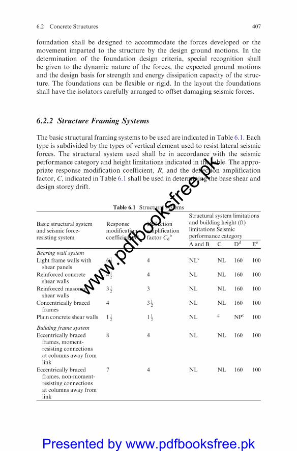
foundation shall be designed to accommodate the forces developed or themovement imparted to the structure by the design ground motions. In thedetermination of the foundation design criteria, special recognition shallbe given to the dynamic nature of the forces, the expected ground motionsand the design basis for strength and energy dissipation capacity of the struc-ture. The foundations can be flexible or rigid. In the layout the foundationsshall have the isolators carefully arranged to offset damaging seismic forces.
6.2.2 Structure Framing Systems
The basic structural framing systems to be used are indicated in Table 6.1. Eachtype is subdivided by the types of vertical element used to resist lateral seismicforces. The structural system used shall be in accordance with the seismicperformance category and height limitations indicated in the table. The appro-priate response modification coefficient, R, and the deflection amplificationfactor, C, indicated in Table 6.1 shall be used in determining the base shear anddesign storey drift.
Table 6.1 Structural systems
Basic structural systemand seismic force-resisting system
Responsemodificationcoefficient Ra
Deflectionamplificationfactor Cd
b
Structural system limitationsand building height (ft)limitations Seismicperformance category
A and B C Dd Ee
Bearing wall system
Light frame walls withshear panels
6 12 4 NLc NL 160 100
Reinforced concreteshear walls
4 12
4 NL NL 160 100
Reinforced masonryshear walls
3 12
3 NL NL 160 100
Concentrically bracedframes
4 3 12
NL NL 160 100
Plain concrete shear walls 1 12
1 12
NL g NPc 100
Building frame system
Eccentrically bracedframes, moment-resisting connectionsat columns away fromlink
8 4 NL NL 160 100
Eccentrically bracedframes, non-moment-resisting connectionsat columns away fromlink
7 4 NL NL 160 100
6.2 Concrete Structures 407
www.pdfbo
oksfr
ee.pk
Presented by www.pdfbooksfree.pk

Table 6.1 (continued)
Basic structural systemand seismic force-resisting system
Responsemodificationcoefficient Ra
Deflectionamplificationfactor Cd
b
Structural system limitationsand building height (ft)limitations Seismicperformance category
A and B C Dd Ee
Composite eccentricallybraced frames(C-EBF)
8 4 NL NL 160 100
Light frame walls withshear panels
7 4 12 NL NL 160 100
Concentrically bracedframes
5 4 12 NL NL 160 100
Composite concentricallybraced frames(C-CBF)
5 4 12
NL NL 160 100
Reinforced concreteshear walls
5 12
5 NL NL 160 100
RC shear wallscomposite with steelelements
5 12
5 NL NL 160 100
Plain (unreinforced)masonry shear walls
1 12
1 12
NL f NP NP
Plain concrete shear walls 2 2 NL g NP NP
Dual system with anintermediate momentframe of reinforcedconcrete or an ordinarymoment frame of steelcapable of resisting atleast 25% of prescribedseismic forces
Concentrically bracedframes
5 4 12
NL NL 160 100
Composite concentricallybraced frames(C-CBF)
5 4 12
NL NL 160 100
Reinforced concreteshear walls
6 5 NL NL 160 100
RC shear wallscomposite with steelelements
6 5 NL NL 160 100
Special moment framesof reinforced concrete
2 12 2 1
2 NL NL NL NL
key 1ft=0.3048m
Note: Data collected from the archives of the British Library and organised them in the givenformat
408 6 Geotechnical Earthquake Engineering and Soil–Structure Interaction
www.pdfbo
oksfr
ee.pk
Presented by www.pdfbooksfree.pk

Table 6.1 (continued)
Basic structural systemand seismic force-resisting system
Responsemodificationcoefficient Ra
Deflectionamplificationfactor Cd
b
Structural system limitationsand building height (ft)limitations Seismicperformance category
A and B C Dd Ee
Moment-resisting framessystem
Special moment framesof reinforced concrete
8 5 NL NL NL NL
Composite specialmoment frames(C-SMF)
8 5 12
NL NL NL NL
Intermediate momentframes of reinforcedconcrete
5 4 12
NL NL NP NP
Composite ordinarymoment frames(C-OMF)
4 12
4 NL NL 160 100
Composite partiallyrestrained frames(C-PRF)
6 5 12
160 160 100 NP
Ordinary moment framesof reinforced concrete
3 2 12
NLh NP NP NP
Dual system with a specialmoment frame capableof resisting at least25% of prescribedseismic forces
Eccentrically bracedframes, moment-resisting
connections at columnsaway from link
8 4 NL NL NL NL
Eccentrically bracedframes, non-momentresisting
connections at columnsaway from link
7 4 NL NL NL NL
Composite eccentricallybraced frames(C-EBF)
8 4 NL NL NL NL
Concentrically bracedframes
6 5 NL NL NL NL
Special concentricallybraced frames– steel
8 6 12
NL NL NL NL
Composite concentricallybraced frames(C-CBF)
6 5 NL NL NL NL
Reinforced concreteshear walls
8 6 12
NL NL NL NL
6.2 Concrete Structures 409
www.pdfbo
oksfr
ee.pk
Presented by www.pdfbooksfree.pk
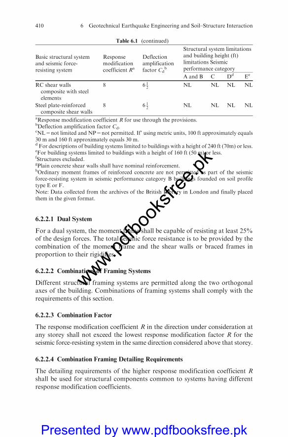
6.2.2.1 Dual System
For a dual system, the moment frame shall be capable of resisting at least 25%of the design forces. The total seismic force resistance is to be provided by thecombination of the moment frame and the shear walls or braced frames inproportion to their rigidities.
6.2.2.2 Combinations of Framing Systems
Different structural framing systems are permitted along the two orthogonalaxes of the building. Combinations of framing systems shall comply with therequirements of this section.
6.2.2.3 Combination Factor
The response modification coefficient R in the direction under consideration atany storey shall not exceed the lowest response modification factor R for theseismic force-resisting system in the same direction considered above that storey.
6.2.2.4 Combination Framing Detailing Requirements
The detailing requirements of the higher response modification coefficient Rshall be used for structural components common to systems having differentresponse modification coefficients.
Table 6.1 (continued)
Basic structural systemand seismic force-resisting system
Responsemodificationcoefficient Ra
Deflectionamplificationfactor Cd
b
Structural system limitationsand building height (ft)limitations Seismicperformance category
A and B C Dd Ee
RC shear wallscomposite with steelelements
8 6 12 NL NL NL NL
Steel plate-reinforcedcomposite shear walls
8 6 12 NL NL NL NL
aResponse modification coefficient R for use through the provisions.bDeflection amplification factor Cd.cNL=not limited and NP=not permitted. If’ using metric units, 100 ft approximately equals30 m and 160 ft approximately equals 30 m.d For descriptions of building systems limited to buildings with a height of 240 ft (70m) or less.eFor building systems limited to buildings with a height of 160 ft (50 m) or less.fStructures excluded.gPlain concrete shear walls shall have nominal reinforcement.hOrdinary moment frames of reinforced concrete are not permitted as part of the seismicforce-resisting system in seismic performance category B buildings founded on soil profiletype E or F.Note: Data collected from the archives of the British Library in London and finally placedthem in the given format.
410 6 Geotechnical Earthquake Engineering and Soil–Structure Interaction
www.pdfbo
oksfr
ee.pk
Presented by www.pdfbooksfree.pk
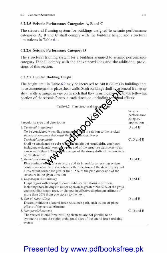
6.2.2.5 Seismic Performance Categories A, B and C
The structural framing system for buildings assigned to seismic performance
categories A, B and C shall comply with the building height and structural
limitations in Table 6.1.
6.2.2.6 Seismic Performance Category D
The structural framing system for a building assigned to seismic performance
category D shall comply with the above provisions and the additional provi-
sions of this section.
6.2.2.7 Limited Building Height
The height limit in Table 6.2 may be increased to 240 ft (70 m) in buildings that
have concrete cast-in-place shear walls. Such buildings shall have braced frames or
shear walls arranged in one plane such that they resist no more than the following
portion of the seismic forces in each direction, including torsional effects:
Table 6.2 Plan structural irregularities
Irregularity type and description
Seismicperformancecategoryapplication
1. Torsional irregularity D and E
To be considered when diaphragms are rigid in relation to the verticalstructural elements that resist the lateral seismic forces
Torsional irregularity C, D and E
Shall be considered to exist when the maximum storey drift, computedincluding accidental torsion, at one end of the structure transverse to anaxis is more than 1.2 times the average of the storey drifts at the two endsof the structure
2. Re-entrant corners D and E
Plan configurations of a structure and its lateral force-resisting systemcontain re-entrant corners, where both projections of the structure beyonda re-entrant corner are greater than 15% of the plan dimension of thestructure in the given direction
3. Diaphragm discontinuity D and E
Diaphragms with abrupt discontinuities or variations in stiffness,including those having cut out or open areas greater than 50% of the grossenclosed diaphragm area, or changes in effective diaphragm stiffness ofmore than 50% from one storey to the next
4. Out-of-plane offsets D and E
Discontinuities in a lateral force resistance path, such as out-of-planeoffsets of the vertical elements
5. Non-parallel systems C, D and E
The vertical lateral force-resisting elements are not parallel to orsymmetric about the major orthogonal axes of the lateral force-resistingsystem
6.2 Concrete Structures 411
www.pdfbo
oksfr
ee.pk
Presented by www.pdfbooksfree.pk
(a) 60% where the braced frame or shear walls are arranged only on theperimeter.
(b) 40% where some of the braced frames or shear walls are arranged on theperimeter.
(c) 30% for other arrangements.
6.2.2.8 Interaction Effects
Moment-resisting frames that are enclosed or adjoined by more rigid elementsnot considered to be part of the seismic force-resisting system shall be analysedand designed so that the action or failure of those elements will not impair thevertical.
6.2.2.9 Deformational Compatibility
Every structural component not included in the seismic force-resisting system inthe direction under consideration shall be designed to be adequate for thevertical loadcarrying capacity and the induced moments resulting from thedesign storey drift.
6.2.2.10 Special Moment Frames
A special moment frame that is used but not required by Table 6.1 is permittedto be discontinued and supported by a more rigid system with a lower responsemodification coefficient. Where a special moment frame is required byTable 6.1., the frame shall be continuous to the foundation.
6.2.2.11 Seismic Performance Category E
The framing systems of buildings assigned to category E shall conform to thecode requirements for category D and to the additional requirements andlimitations of this section. The height limitation shall be reduced from 240 to160 ft (from 70 to 50 m).
6.2.2.12 Seismic Building Configuration
Buildings shall be classified as regular or irregular based on the criteria in thissection. Such classification shall be based on the plan and vertical configuration.
6.2.2.13 Plan Irregularity
Buildings having one or more of the features given in Table 6.2 shall bedesignated as having plan structural irregularity and shall comply with therequirements in the codes.
412 6 Geotechnical Earthquake Engineering and Soil–Structure Interaction
www.pdfbo
oksfr
ee.pk
Presented by www.pdfbooksfree.pk
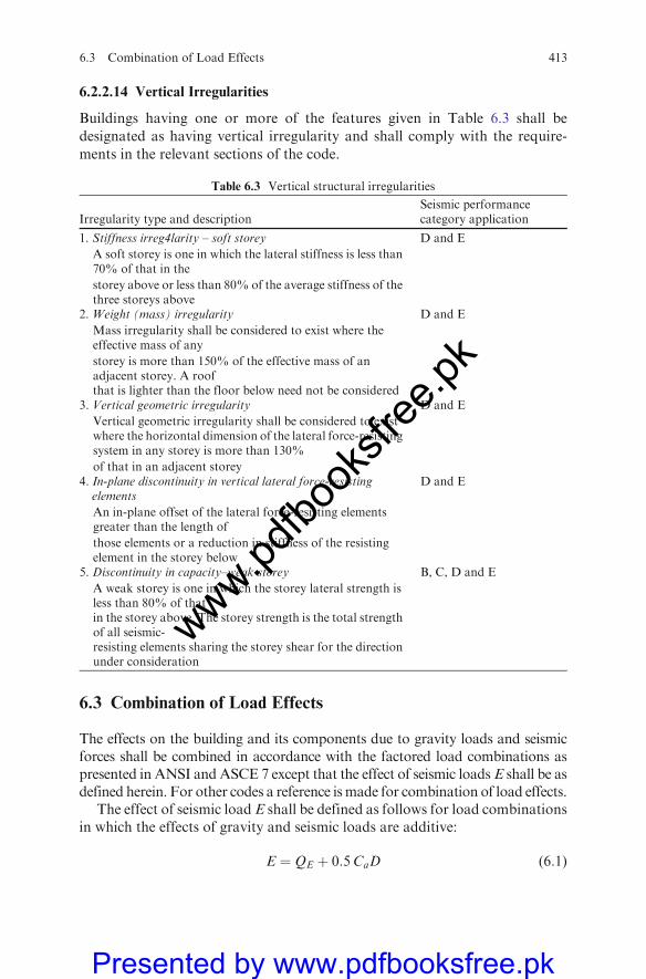
6.2.2.14 Vertical Irregularities
Buildings having one or more of the features given in Table 6.3 shall be
designated as having vertical irregularity and shall comply with the require-
ments in the relevant sections of the code.
6.3 Combination of Load Effects
The effects on the building and its components due to gravity loads and seismicforces shall be combined in accordance with the factored load combinations aspresented in ANSI and ASCE 7 except that the effect of seismic loads E shall be asdefined herein. For other codes a reference ismade for combination of load effects.
The effect of seismic load E shall be defined as follows for load combinationsin which the effects of gravity and seismic loads are additive:
E ¼ QE þ 0:5CaD (6:1)
Table 6.3 Vertical structural irregularities
Irregularity type and descriptionSeismic performancecategory application
1. Stiffness irreg4larity – soft storey D and E
A soft storey is one in which the lateral stiffness is less than70% of that in the
storey above or less than 80% of the average stiffness of thethree storeys above
2. Weight (mass) irregularity D and E
Mass irregularity shall be considered to exist where theeffective mass of any
storey is more than 150% of the effective mass of anadjacent storey. A roofthat is lighter than the floor below need not be considered
3. Vertical geometric irregularity D and E
Vertical geometric irregularity shall be considered to existwhere the horizontal dimension of the lateral force-resistingsystem in any storey is more than 130%
of that in an adjacent storey4. In-plane discontinuity in vertical lateral force-resistingelements
D and E
An in-plane offset of the lateral force-resisting elementsgreater than the length of
those elements or a reduction in stiffness of the resistingelement in the storey below
5. Discontinuity in capacity–weak storey B, C, D and E
A weak storey is one in which the storey lateral strength isless than 80% of thatin the storey above. The storey strength is the total strengthof all seismic-resisting elements sharing the storey shear for the directionunder consideration
6.3 Combination of Load Effects 413
www.pdfbo
oksfr
ee.pk
Presented by www.pdfbooksfree.pk
where E is the effect of horizontal and vertical earthquake-induced forces; Ca ’’
is the seismic coefficient based on the soil profile type and the values of Ca asdetermined;D is the effect of dead load andQE is the effect of horizontal seismicforces.
The effect of seismic load E shall be defined by (6.2) as follows for loadcombinations in which the effects of gravity counteract seismic load:
E ¼ QE � 0:5CaD (6:2)
where E, QE, Ca and D are as defined above.The load factor on E need not be taken as greater than 1.0 in factored load
combinations when using the seismic loads as defined in these provisions.For columns supporting discontinuous lateral force-resisting elements, the
axial force in the columns shall be computed using the most critical load
combinations. Load combinations including seismic loads shall also be inves-tigated, except that the effect of seismic load E shall be defined by (6.3) asfollows:
E ¼ 2R
5
� �QE þ 0:5CaD (6:3)
where E,QE, Ca andD are as defined above and R is the response modificationcoefficient as given in Table 6.1. The axial forces in such columns need notexceed the capacity of other elements of the structure to transfer such loads tothe column.
Brittle materials, systems and connections shall be designed using the mostcritical load combinations. Load combinations including seismic loads shallalso be investigated, except that the effect of seismic load E shall be defined by(6.6) as follows:
E ¼ 2R
5
� �QE � 0:5CaD (6:4)
where E, R, QE, Ca and D are as defined above.The factor (2 R/5) shall be equal to or greater than 1.0. The term 0.5 Ca is
permitted.
6.4 Deflection and Drift Limits
The design storey drift D as determined shall not exceed the allowable storeydrift Da as obtained for any torsional effects (Table 6.4). All portions of thebuilding shall be designed and constructed to act as an integral unit in resisting
414 6 Geotechnical Earthquake Engineering and Soil–Structure Interaction
www.pdfbo
oksfr
ee.pk
Presented by www.pdfbooksfree.pk

seismic forces unless separated structurally by a distance sufficient to avoiddamaging contact under total deflection.
6.5 Equivalent Lateral Force Procedure
6.5.1 General
This section provides the requiredminimum standards for the equivalent lateralforce procedure of seismic analysis of buildings. For purposes of analysis, thebuilding is considered to be fixed at the base.
6.5.2 Seismic Base Shear
The seismic base shear V in a given direction shall be determined in accordancewith the following equation:
V ¼ C3W (6:5)
where C3 is the seismic response coefficient and W is the total dead load andapplicable portions of other loads listed below.
(a) In areas used for storage, a minimum of 25% of the floor live load shall beapplicable. Floor live load in public garages and open parking structures isnot applicable.
Table 6.4 Allowable storey drift Da (in or mm)
Building
Seismic Hazard Exposure group
I II III
Buildings, other than masonry shear wall ormasonry wall frame buildings, four storeysor less in height with interior walls,partitions, ceilings and exterior wall systemsthat have been designed to accommodate thestorey drifts
0.025 hsxa,b 0.020 hsx 0.015 hsx
Masonry cantilever shear wall buildings 0.010 hsx 0.010 hsxc 0.010 hsx
Other masonry shear wall buildings 0.007 hsx 0.007 hsxc 0.007 hsx
Masonry wal4 frame buildings 0.010 hsxc 0.013 hsx 0.010 hsx
All other buildings 0.020 hsx 0.015 hsx 0.010 hsxa hsx is the storey height below level x.b There shall be no drift limit for single-storey buildings with interior wall partitions, ceilingsand exterior wall systems that have been designed to accommodate the storey drifts.cBuildings in which the basic structural system consists of masonry shear walls designed asvertical elements cantilevered from their base foundation support which are so constructedthat moment transfer between shear walls (coupling) is negligible. Data collected from theLibrary of ASCE, (U.S.A.)
6.5 Equivalent Lateral Force Procedure 415
www.pdfbo
oksfr
ee.pk
Presented by www.pdfbooksfree.pk
(b) Where an allowance for particular load is included in the floor load design,the actual partition weight or a minimum weight of 10 psf (0.5 kN/m2) offloor area, whichever is greater, shall be applicable.
(c) Total operating weight of permanent equipment.
6.5.2.1 Calculation of Seismic Response Coefficient
When the fundamental period of the building is computed, the seismic responsecoefficient CS; shall be determined in accordance with the following equation:
CS ¼ ð1:2CVÞÞ=ðRT2=3Þ (6:6)
where
CV=the seismic coefficient based on the soil profile type and the value ofAV
R = the response modification factorT = the fundamental period of the building (s).
A soil–structure interaction reduction is permitted when determined usingthe generally accepted procedures approved by the regulatory agency.
Alternatively, the seismic response coefficient need not be greater than thefollowing:
CS ¼ ð2:5CVÞ=R (6:7)
whereR is as above andCs is the seismic coefficient based on the soil profile typeand the value of Aa.
6.5.3 Period Determination
The fundamental period T of the building in the direction under considerationshall be established using the structural properties and deformational charac-teristics of the resisting elements in a properly substantiated analysis. Thefundamental period T shall not exceed the product of the coefficient for upperlimit on calculated period Cu from Table 6.5 and the approximate fundamentalperiod Ta determined from the appropriate requirements.
6.5.3.1 I Approximate Fundamental Period for Concrete and Steel
Moment-Resisting Frame Buildings
The approximate fundamental period, Ta in seconds, shall be determined fromthe following equation:
Ta ¼ CTh3=4n (6:8)
416 6 Geotechnical Earthquake Engineering and Soil–Structure Interaction
www.pdfbo
oksfr
ee.pk
Presented by www.pdfbooksfree.pk
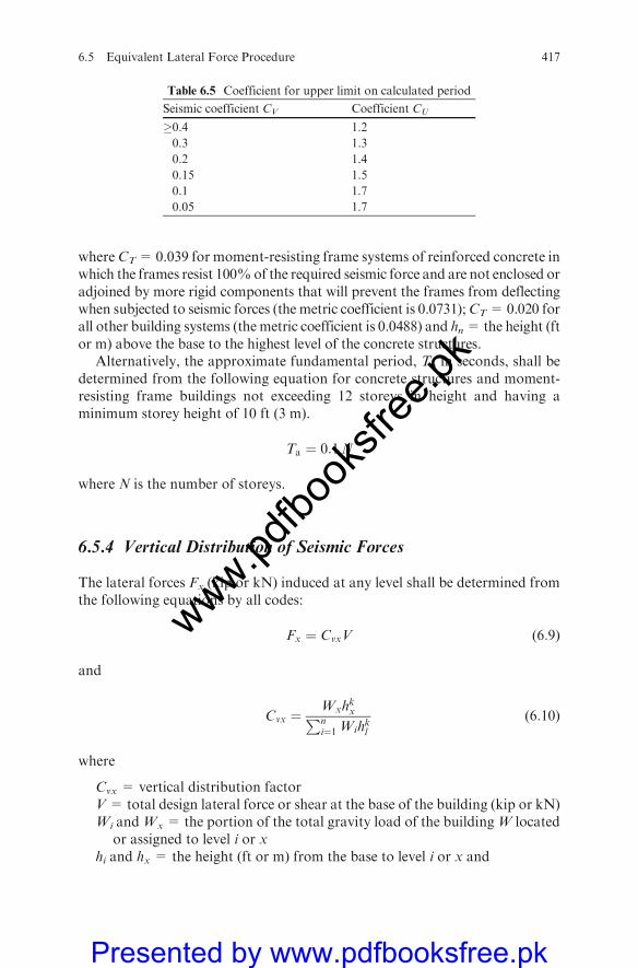
whereCT=0.039 for moment-resisting frame systems of reinforced concrete inwhich the frames resist 100%of the required seismic force and are not enclosed oradjoined by more rigid components that will prevent the frames from deflectingwhen subjected to seismic forces (the metric coefficient is 0.0731);CT=0.020 forall other building systems (themetric coefficient is 0.0488) and hn= the height (ftor m) above the base to the highest level of the concrete structures.
Alternatively, the approximate fundamental period, Ta in seconds, shall bedetermined from the following equation for concrete structures and moment-resisting frame buildings not exceeding 12 storeys in height and having aminimum storey height of 10 ft (3 m).
Ta ¼ 0:1N
where N is the number of storeys.
6.5.4 Vertical Distribution of Seismic Forces
The lateral forces Fx (kip or kN) induced at any level shall be determined fromthe following equations by all codes:
Fx ¼ CvxV (6:9)
and
Cvx ¼Wxh
kxPn
i¼1 Wihkl
(6:10)
where
Cvx = vertical distribution factorV= total design lateral force or shear at the base of the building (kip or kN)Wi andWx = the portion of the total gravity load of the buildingW located
or assigned to level i or xhi and hx = the height (ft or m) from the base to level i or x and
Table 6.5 Coefficient for upper limit on calculated period
Seismic coefficient CV Coefficient CU
�0.4 1.2
0.3 1.3
0.2 1.4
0.15 1.5
0.1 1.7
0.05 1.7
6.5 Equivalent Lateral Force Procedure 417
www.pdfbo
oksfr
ee.pk
Presented by www.pdfbooksfree.pk
K= an exponent related to the building period as follows:For buildings having a period of 0.5 s or less, k=1for buildings having a period of 2.5 s or less, k = 1for buildings having a period between 0.5 and 2.5 s, k shall be 2 or shall be
determined by linear interpolation between 1 and 2.
6.6 Horizontal Shear Distribution
The seismic design storey shear in any storeyVx (kip or kN) shall be determined
from the following equation:
Vx ¼ SxFi (6:11)
where Fi is the portion of the seismic base shearV (kip or kN) induced at level i.The seismic design storey, Vx (kip or kN), shall be distributed to the various
vertical elements of the seismic force-resisting system in the storey under con-
sideration, based on the relative lateral stiffness of the vertical-resisting ele-
ments and the diaphragm.
6.6.1 Torsion
The design shall include the torsional moment, M (kip-ft or kNm), resulting
from the location of the structure (masses plus the accidental torsional
moments, Mta (kip-ft or kNm)) caused by assumed displacement of the base
each way from its actual location by a distance equal to 5% of the dimension of
the building perpendicular to the direction of the applied forces.Buildings of seismic performance categories C, D and E, where type 1
torsional irregularity exists. shall have the effects accounted for by increasing
the accidental torsion at each level by a torsional amplification factor Ax
determined from the following equation
Ax ¼dmax
1:2 davg
� �(6:12)
where dmax is the maximum displacement at level x (in or mm) and davg is theaverage of the displacements at the extreme points of the structure at level x (in
or mm).The torsional amplification factorAx is not required to exceed 3.0. The more
severe loading for each element shall be considered for design.
418 6 Geotechnical Earthquake Engineering and Soil–Structure Interaction
www.pdfbo
oksfr
ee.pk
Presented by www.pdfbooksfree.pk
6.6.2 Overturning (determined by all codes)
The building shall be designed to resist overturning effects caused by the seismicforces. At any storey, the increment of overturning moment in the storey underconsideration shall be distributed to the various vertical force-resisting elements inthe same proportion as the distribution of the horizontal shears to those elements.
The overturningmoments at level x,Mx (kip-ft or kNm), shall be determinedfrom the following equation:
Mx ¼ tSni¼xFiðhi ¼ hxÞ (6:13)
where
Fi = the position of the seismic base shear V included at level i,hi and hx = the height (ft or m) from the base to level i or x,t = 1.0 for the top 10 storeys,t = 0.8 for the 20th storey from the top and below, andt = a value between 1.0 and 0.8 determined by a straight line interpolation
for storeys between the 20th and 10th storeys below the top.
The foundations of buildings except inverted-type structures shall bedesigned for the foundation overturning design moment, M (kip-ft or kNrn),at the foundation soil interface determined using the equation for the over-turning moment at level M (kip-ft or kNm) with an overturning momentreduction factor T of 0.75 for all building heights.
6.7 Drift Determination and P�D Effects
Storey drifts and, where required, member forces and moments due to P� Deffects shall be determined in accordance with this section.
6.7.1 Storey Drift Determination (determined by all codes)
The design storey drift shall be computed as the difference between the deflec-tions at the top and bottom of the storey under consideration. The deflections oflevel x at the centre of the mass, dx (in or mm), shall be determined in accor-dance with the following equation:
dx ¼ Cddxc (6:14)
where
Cd = the deflection amplification factordxc= the deflections determined by an elastic analysis (in or mm)
6.7 Drift Determination and P�D Effects 419
www.pdfbo
oksfr
ee.pk
Presented by www.pdfbooksfree.pk

Where applicable, the design storey drift, D (in or mm) shall be increased bythe incremental factor relating to the P� D effects.
6.7.2 P�D Effects (determined according to all codes)
P� D effects on storey shears and moments the resulting member forces andmoments, and the storey drifts induced by these effects are not required to beconsidered when the stability coefficient y, as determined by the followingequation, is equal to or less than 0.10:
y ¼ ðPxDÞ=ðVxhsxCdÞ (6:14a)
where
Px = the total vertical design load at and above level x (kip or kN); whencalculating the vertical design load for purposes of determining P� Dthe individual load factors need not exceed 1.0
D= the design storey drift occurring simultaneously with V� (in or mm)Vx = the seismic shear force acting between level x and x�1 (kip or kN)hsx = the storey height below level x (ft or m)Cd = the deflection amplification factor
The stability coefficient B shall not exceed ymax determined as follows:
ymax ¼ 0:5=ðbCdÞ � 0:25 (6:14b)
where b is the ratio of shear demand to shear capacity for the storey betweenlevel x and x�1. The ratio may be conservatively taken as 1.0.
When the stability coefficient y is greater than 0.10 but less than or equal toymax the incremental factor is related to P�D.
To obtain the storey drift for including theP�D effect, the design storey driftdetermined shall be multiplied by 1.0/(1 � y). When y is greater than ymax thestructure is potentially unstable and shall be redesigned.
6.8 Modal Analysis Procedure: Codified Approach
6.8.1 Introduction
A reference is made to themodel analysis in Chap. 4 with examples. This sectionprovides required standards for the modal analysis procedures of seismic ana-lysis of structures. The symbols used in this method of analysis have the samemeaning as those for similar terms with the subscript m denoting quantities inthe mth mode. The structure shall be modelled as a system of masses lumped at
420 6 Geotechnical Earthquake Engineering and Soil–Structure Interaction
www.pdfbo
oksfr
ee.pk
Presented by www.pdfbooksfree.pk
various levels with each mass having one degree of freedom – that of lateraldisplacement in the direction under consideration.
The analysis shall include, for each of two mutually perpendicular axes, atleast the lowest three modes of vibration or all modes of vibration with periodsgreater than 0.4 s. The number of modes shall equal the number of storeys forbuildings less than three storeys in height.
The required periods and mode shapes of the building in the direction underconsideration shall be calculated by established methods of structural analysisfor the fixed–base condition using the masses and elastic stiffnesses of theseismic force–resisting system. A reference is made to Chap. 5 for modal andChap. 6 for other analyses and solution procedures.
6.8.2 Modal Base Shear as by Codified Methods
The portion of the base shear contributed by the mth mode, Vm, shall bedetermined from the following equations:
Vm ¼ Csm�Wn (6:15)
�Wm ¼Pn
i¼l wifim
� �Pn
i¼l wif2im
(6:16)
where
Csm = the modal seismic response coefficient determined belowWm = the effective modal gravitywi = the portion of the total gravity load of the building at level i and
fim = the displacement amplitude at the ith level of the building whenvibrating in its mth mode.
The modal seismic response coefficient Csm shall be determined in accor-dance with the following equation:
Csm ¼ ð1:2CvÞ=ðRT 2=3m Þ (6:17)
where
Cv = the seismic coefficient based on the soil profile type and the value Av
R = the response modification factor determined from Table 6.1 andTm = the modal period of vibration (in seconds) of the mth mode of the
building.
The modal seismic design coefficient Csm is not required to exceed 2.5 timesthe seismic coefficient Ca divided by the response modification factor R.
The following are the exceptions.
6.8 Modal Analysis Procedure: Codified Approach 421
www.pdfbo
oksfr
ee.pk
Presented by www.pdfbooksfree.pk
(a) The limiting value is not applicable to seismic performance category 0 and Ebuildings with a period of 0.7 s or greater located on soil profile type E or Fsites.
(b) For buildings on sites with soil profile type D, E or F, the modal seismicdesign coefficient Csm for modes other than the fundamental mode thathave periods less than 0.3 s is permitted to be determined by the followingequation:
Csm ¼Ca
Rð1:0þ 5:0TmÞ; (6:18)
whereR and Tm are as defined above andCa is the seismic coefficient basedon the soil profile type and the value of Aa.
(c) For buildings where any modal period of vibration Tm exceeds 4.0 s, themodal seismic design coefficient Csm for that mode is permitted to bedetermined by the following equation:
Csm ¼3Ca
RT4=3m
(6:19)
where R and Tm are as defined above and Ca is the seismic coefficient based onthe soil type and the value of Av.
The reduction due to soil structure–concrete interaction may be used.
6.8.3 Modal Forces, Deflection and Drifts
The modal force Fxm at each level shall be determined by the followingequations:
Fvm ¼ CvxmVm (6:20)
and
Cvxm ¼wxfvmPni¼l wifim
(6:21)
where Cvsm = the vertical factor in the mth mode except that for buildingswhere the gravity load is concentrated at a single level, it shall be taken as equalto W.
The reduced based shear V shall in no case be taken as less than 0.7 V.
Vm = the total design lateral force or shear at the base in the mth modewi,wx = the portion of the total gravity load of the building W located or
assigned to level i or x
422 6 Geotechnical Earthquake Engineering and Soil–Structure Interaction
www.pdfbo
oksfr
ee.pk
Presented by www.pdfbooksfree.pk
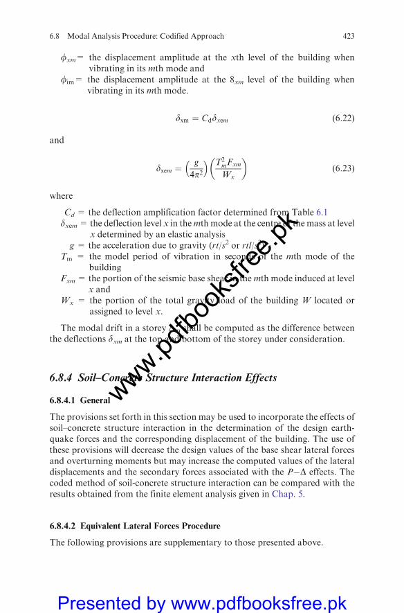
fxm= the displacement amplitude at the xth level of the building whenvibrating in its mth mode and
fim= the displacement amplitude at the 8xm level of the building whenvibrating in its mth mode.
dxm ¼ Cddxem (6:22)
and
dxem ¼g
4p2
� � T2mFxm
Wx
� �(6:23)
where
Cd = the deflection amplification factor determined from Table 6.1dxem=the deflection level x in themth mode at the centre of the mass at level
x determined by an elastic analysisg = the acceleration due to gravity (rt/s2 or rtl/s2)
Tm = the model period of vibration in seconds of the mth mode of thebuilding
Fxm = the portion of the seismic base shear in themth mode induced at levelx and
Wx = the portion of the total gravity load of the building W located orassigned to level x.
The modal drift in a storey Dm shall be computed as the difference betweenthe deflections dxm at the top and bottom of the storey under consideration.
6.8.4 Soil–Concrete Structure Interaction Effects
6.8.4.1 General
The provisions set forth in this section may be used to incorporate the effects ofsoil–concrete structure interaction in the determination of the design earth-quake forces and the corresponding displacement of the building. The use ofthese provisions will decrease the design values of the base shear lateral forcesand overturning moments but may increase the computed values of the lateraldisplacements and the secondary forces associated with the P�D effects. Thecoded method of soil-concrete structure interaction can be compared with theresults obtained from the finite element analysis given in Chap. 5.
6.8.4.2 Equivalent Lateral Forces Procedure
The following provisions are supplementary to those presented above.
6.8 Modal Analysis Procedure: Codified Approach 423
www.pdfbo
oksfr
ee.pk
Presented by www.pdfbooksfree.pk
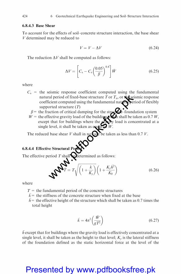
6.8.4.3 Base Shear
To account for the effects of soil–concrete structure interaction, the base shearV determined may be reduced to
V ¼ V� DV (6:24)
The reduction DV shall be computed as follows:
DV ¼ Cs � Cs0:05
b
� �0:4" #
�W (6:25)
where
Cs = the seismic response coefficient computed using the fundamentalnatural period of fixed-base structure T or Ta, or the seismic responsecoefficient computed using the fundamental natural period of flexiblysupported structure (T)
b= the fraction of critical damping for the structure–foundation systemW= the effective gravity load of the building which shall be taken as 0.7W,
except that for buildings where the gravity load is concentrated at asingle level, it shall be taken as equal to W.
The reduced base shear V shall in no case be taken as less than 0.7 V.
6.8.4.4 Effective Structural Period
The effective period T shall be determined as follows:
�T ¼ T
ffiffiffiffiffiffiffiffiffiffiffiffiffiffiffiffiffiffiffiffiffi1þ k
Ky
� �s1þ Ky
�h2
K0
� �(6:26)
where
T = the fundamental period of the concrete structures�k= the stiffness of the concrete structure when fixed at the base�h= the effective height of the structure which shall be taken as 0.7 times thetotal height
�k ¼ 4p2�W
gT2
� �(6:27)
�h except that for buildings where the gravity load is effectively concentrated at asingle level, it shall be taken as the height to that level; Ky is the lateral stiffnessof the foundation defined as the static horizontal force at the level of the
424 6 Geotechnical Earthquake Engineering and Soil–Structure Interaction
www.pdfbo
oksfr
ee.pk
Presented by www.pdfbooksfree.pk
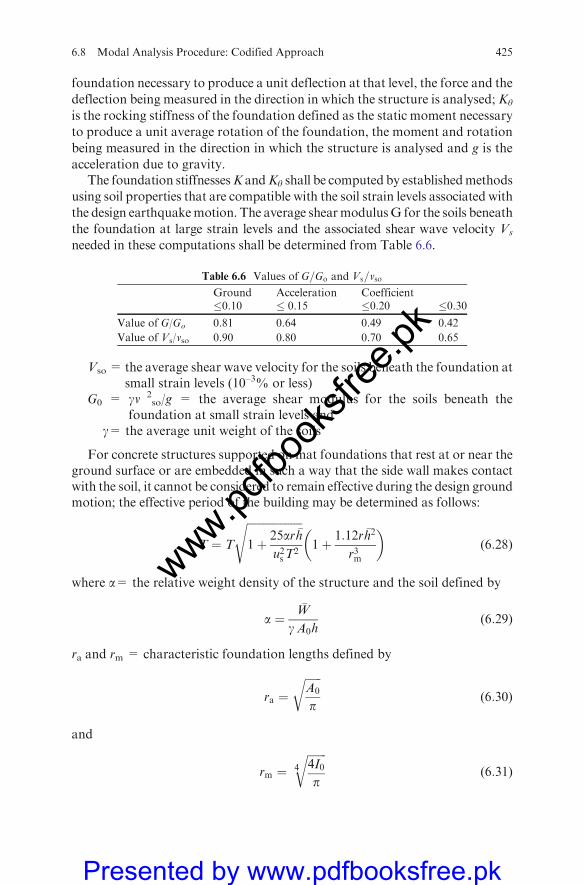
foundation necessary to produce a unit deflection at that level, the force and the
deflection being measured in the direction in which the structure is analysed; Ky
is the rocking stiffness of the foundation defined as the static moment necessary
to produce a unit average rotation of the foundation, the moment and rotation
being measured in the direction in which the structure is analysed and g is the
acceleration due to gravity.The foundation stiffnessesK andKy shall be computed by establishedmethods
using soil properties that are compatible with the soil strain levels associated with
the design earthquakemotion. The average shearmodulusG for the soils beneath
the foundation at large strain levels and the associated shear wave velocity Vs
needed in these computations shall be determined from Table 6.6.
Vso= the average shear wave velocity for the soils beneath the foundation atsmall strain levels (10–3% or less)
G0 = gv 2so/g = the average shear modulus for the soils beneath the
foundation at small strain levels andg= the average unit weight of the soils
For concrete structures supported on mat foundations that rest at or near theground surface or are embedded in such a way that the side wall makes contactwith the soil, it cannot be considered to remain effective during the design groundmotion; the effective period of the building may be determined as follows:
T ¼ T
ffiffiffiffiffiffiffiffiffiffiffiffiffiffiffiffiffiffiffiffi1þ 25ar �h
u2sT2
s1þ 1:12r �h2
r3m
� �(6:28)
where a= the relative weight density of the structure and the soil defined by
a ¼�W
gA0h(6:29)
ra and rm = characteristic foundation lengths defined by
ra ¼ffiffiffiffiffiffiA0
p
r(6:30)
and
rm ¼ 4
ffiffiffiffiffiffiffi4I0p
r(6:31)
Table 6.6 Values of G=Go and Vs=vso
Ground Acceleration Coefficient�0.10 � 0.15 �0.20 �0.30
Value of G/Go 0.81 0.64 0.49 0.42
Value of Vs/vso 0.90 0.80 0.70 0.65
6.8 Modal Analysis Procedure: Codified Approach 425
www.pdfbo
oksfr
ee.pk
Presented by www.pdfbooksfree.pk
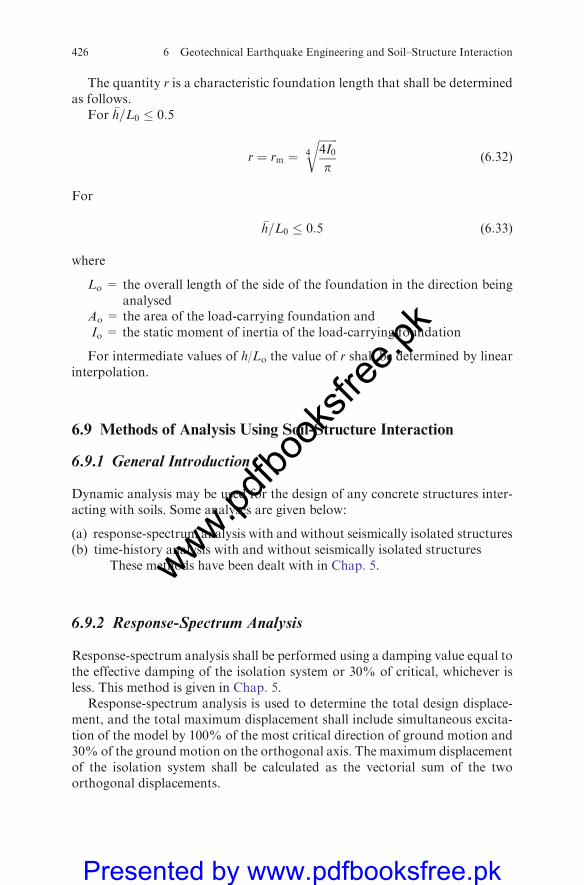
The quantity r is a characteristic foundation length that shall be determinedas follows.
For �h=L0 � 0:5
r ¼ rm ¼ 4
ffiffiffiffiffiffiffi4I0
p
r(6:32)
For
�h=L0 � 0:5 (6:33)
where
Lo = the overall length of the side of the foundation in the direction beinganalysed
Ao = the area of the load-carrying foundation andIo = the static moment of inertia of the load-carrying foundation
For intermediate values of h/Lo the value of r shall be determined by linearinterpolation.
6.9 Methods of Analysis Using Soil-Structure Interaction
6.9.1 General Introduction
Dynamic analysis may be used for the design of any concrete structures inter-acting with soils. Some analyses are given below:
(a) response-spectrum analysis with and without seismically isolated structures(b) time-history analysis with and without seismically isolated structures
These methods have been dealt with in Chap. 5.
6.9.2 Response-Spectrum Analysis
Response-spectrum analysis shall be performed using a damping value equal tothe effective damping of the isolation system or 30% of critical, whichever isless. This method is given in Chap. 5.
Response-spectrum analysis is used to determine the total design displace-ment, and the total maximum displacement shall include simultaneous excita-tion of the model by 100% of the most critical direction of ground motion and30% of the groundmotion on the orthogonal axis. The maximum displacementof the isolation system shall be calculated as the vectorial sum of the twoorthogonal displacements.
426 6 Geotechnical Earthquake Engineering and Soil–Structure Interaction
www.pdfbo
oksfr
ee.pk
Presented by www.pdfbooksfree.pk
The design shear at any storey shall not be less than the storey shear obtainedusing the value of Vs taken as equal to the base shear obtained from theresponse-spectrum analysis of the direction of interest.
6.9.3 Time-History Analysis
Time-history analysis shall be performed with at least three appropriate pairs ofhorizontal time-history components as defined.
Each pair of time histories shall be applied simultaneously to the model,considering the most disadvantageous location of mass eccentricity. The max-imum displacement of the isolation system shall be calculated from the vectorialsum of the two orthogonal components at each time step.
The parameter of interest shall be calculated for each time-history analysis. Ifthree time-history analyses are performed, the maximum response of the para-meter of interest shall be used for design. If seven or more time-history analysesare performed, the average value of the response parameter of interest shall beused for design. For each pair of horizontal ground of components, the squareroot sum of the squares (SRSS) of the 5% damped spectrum of the scaledhorizontal components shall be constructed. The motions shall be scaled suchthat the average value of the SRSS spec4ra does not fall below 1.3 times the 5%damped spectrum of the design earthquake (or maximum capable earthquake)by more than 10% in the period range of TI from minus 1.0 s to TI plus 1.0.
Time histories developed for sites within 15 km of a major active fault shallincorporate near-fault phenomena. In both cases the analyses shall be per-formed using specific earthquake input.
The design earthquake shall be used to calculate the total design displace-ment of the isolation system and the lateral forces and displacements of theisolated structure. The maximum capable earthquake shall be used to calculatethe total maximum displacement of the isolation system. The details of thismethod are given in Chap. 5.
6.9.4 Characteristics of Interaction
The interaction effects in the approach used here are expressed by an increase inthe fundamental natural period of the structure and a change (usually anincrease) in its effective damping. The increase in period results from theflexibility of the foundation soil, whereas the change in damping results mainlyfrom the effects of energy dissipation in the soil due to radiation and materialdamping. These statements can be clarified by comparing the responses ofrigidity and elastically supported systems subjected to a harmonic excitationof the base. Consider a linear structure of weight W, lateral stiffness k andcoefficient of viscous damping c (shown in Fig. 6.1) and assume that it is
6.9 Methods of Analysis Using Soil-Structure Interaction 427
www.pdfbo
oksfr
ee.pk
Presented by www.pdfbooksfree.pk
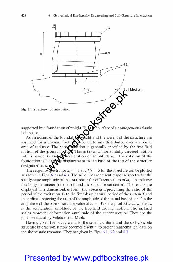
supported by a foundation of weightW0 at the surface of a homogeneous elastichalf-space.
As an example, the foundation weight and the weight of the structure areassumed for a circular footing to be uniformly distributed over a circulararea of radius r. The base excitation is generally specified by the free-fieldmotion of the ground surface. This is taken as horizontally directed motionwith a period T0 and an acceleration of amplitude am. The rotation of thefoundation is y and the displacement to the base of the top of the structuredesignated as u.
The response spectra for h/r=1 and h/r=5 for the structure can be plottedas shown in Figs. 6.2 and 6.3. The solid lines represent response spectra for thesteady-state amplitude of the total shear for different values of f0 –the relativeflexibility parameter for the soil and the structure concerned. The results aredisplayed in a dimensionless form, the abscissa representing the ratio of theperiod of the excitation T0 to the fixed-base natural period of the system T andthe ordinate showing the ratio of the amplitude of the actual base shearV to theamplitude of the base shear. The value of m=W/g in a product mam where amis the acceleration amplitude of the free-field ground motion. The inclinedscales represent deformation amplitude of the superstructure. They are theplots produced by Veletsos and Meek.
Having given the background to the seismic criteria and the soil–concretestructure interaction, it now becomes essential to present mathematical data onthe site seismic response. They are given in Figs. 6.1, 6.2 and 6.3.
uw
k,c
θ (t )
r
h
w
d (t ) Soil Medium
Fig. 6.1 Structure–soil interaction
428 6 Geotechnical Earthquake Engineering and Soil–Structure Interaction
www.pdfbo
oksfr
ee.pk
Presented by www.pdfbooksfree.pk
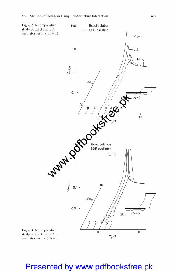
h/r =1
1/3
0.2
φo= 0
0.1
SDF
Exact solution100
10
1
0.1
101
SDF oscillator
V/m
dm
u/dm
55
10
22 1
To / T
Fig. 6.2 A comparativestudy of exact and SDFoscillator result (h/r= 1)
0.1
SDF
Exact solution10
1
0.1
0.01
101
SDF oscillator
55 22 1
10
h/r = 5
φo= 0
V/m
dm
u/dm
To / T
Fig. 6.3 A comparativestudy of exact and SDFoscillator results (h/r= 5)
6.9 Methods of Analysis Using Soil-Structure Interaction 429
www.pdfbo
oksfr
ee.pk
Presented by www.pdfbooksfree.pk
6.10 Site Response – A Critical Problem in Soil–Structure
Interaction Analyses for Embedded Structures
6.10.1 Vertical Earthquake Response and P�D Effect
The methodology for vertical and horizontal response analysis is the same inprinciple. However, the difference in vibrational properties of the structure hasstr4ng influences in response analysis. At least the following three influencesexist.
First, the amplitude and spectral contents of earthquake motion vary withthe magnitude and distance of the earthquake, but differently in the horizontaland vertical directions; the relative amplitude of the vertical motion is higher forsites in the epicentral region.
Second, the possible variation for both amplitude and frequency content is tobe considered when analysing the response in the vertical direction.
Third, the vertical vibration response of vertical members is mainly fromaxial forces while the horizontal response is from the shear and bending forces.The hysteretic property for different loads may be different, especially in thenon-linear range; the P�D effect will produce a descending branch in theforce–deformation curve.
6.10.2 P�D Effects
In an elastic system, P–D may also introduce non-linearity. This effect is veryimportant for high-rise structures and inelastic structures.
For a single mass system as shown in Fig. 6.4 the P�D effect is the secondarymoment produced by the axial force F(t) and the vertical inertial forceM(€vþ €vg) on the deflection u, which is equivalent to an additional horizontalforce
½FðtÞ þMð€vþ €vgÞ�u=H (6:34)
where €vg is the vertical ground acceleration and €v is the relative vertical accel-eration of the mass. Because vertical vibration is also considered, there are nowtwo degrees of freedom and two equations of motion
M€uþ Cu€uþ Ku ¼ PðtÞ �M€ug � ½FðtÞ þMð€vþ €vgÞ�u=H (6:35)
M€vþ Cv _vþ kvv ¼ FðtÞ �M€vg (6:36)
where Cu, Cv are, respectively, the damping coefficient and stiffness of thesystem in the horizontal and vertical directions. It is seen here that the lastterm in (6.38) makes the problem non-linear.
430 6 Geotechnical Earthquake Engineering and Soil–Structure Interaction
www.pdfbo
oksfr
ee.pk
Presented by www.pdfbooksfree.pk
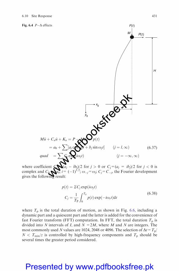
M€uþ Cu _uþ Ku ¼ P�M _ug ¼ pðtÞ
¼ a0 þX½aj cosojtþ bj sinojt� ðj ¼ l;1Þ
quad ¼X
Cj expðiojtÞ ðj ¼ �1;1Þ
(6:37)
where coefficient Cj= (aj � ibj)/2 for j > 0 or Cj=(aj = ibj)/2 for j < 0 iscomplex and C0 = a0; i= (�1)1/2; o�j=oj; Cj=C�j, the Fourier developmentgives the following result:
pðtÞ ¼ SCj expðiojtÞ
Cj ¼l
TP
Z Tp
0
pðtÞ expð�iottÞdt(6:38)
where Tp is the total duration of motion, as shown in Fig. 6.6, including adynamic part and a quiescent part and the latter is added for the convenience offast Fourier transform (FFT) computation. In FFT, the total duration Tp isdivided into N intervals of I, and N =2M, where M and N are integers. Themost commonly usedN values are 1024, 2048 or 4096. The selection of Dt=Tp/N < Tmin/z is controlled by high-frequency components and Tp should beseveral times the greater period considered.
x
H
P(t )
F(t )
yg
xg
M
Fig. 6.4 P�D effects
6.10 Site Response 431
www.pdfbo
oksfr
ee.pk
Presented by www.pdfbooksfree.pk
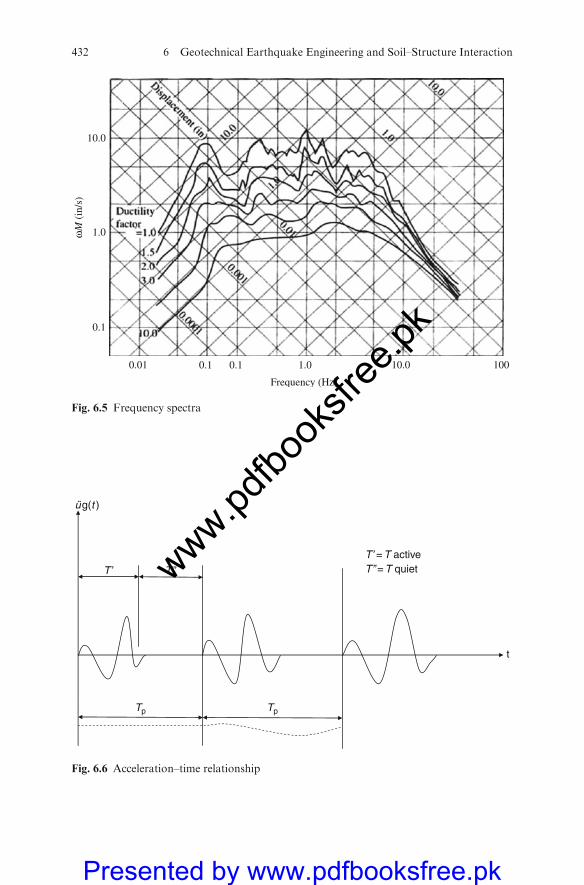
0.01
0.1
1.0ωM
(in
/s)
10.0
0.1 0.1 1.0
Frequency (Hz)
10.0 100
Fig. 6.5 Frequency spectra
T’
T’ = T activeT’’ = T quiet
üg(t )
T’’
TpTp
t
Fig. 6.6 Acceleration–time relationship
432 6 Geotechnical Earthquake Engineering and Soil–Structure Interaction
www.pdfbo
oksfr
ee.pk
Presented by www.pdfbooksfree.pk
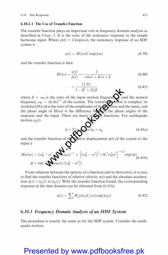
6.10.2.1 The Use of Transfer Function
The transfer function plays an important role in frequency domain analysis asdescribed in Chap. 5. It is the ratio of the stationary response to the simpleharmonic input. Where p(t) = Cexp(iot), the stationary response of an SDFsystem is
uðtÞ ¼ HðioÞC expðiotÞ (6:39)
and the transfer function is then
HðioÞ ¼ uðtÞpðtÞ ¼
1
�mo2 þ iCoþ k(6:40)
¼ ð1=kÞ1� b2 þ 2ixb
(6:41)
where b = o0 is the ratio of the input motion frequency o and the naturalfrequency o0 = (k/m)1/2 of the system. The transfer function is complex; itsmodulus [H(io)] is the ratio of the amplitudes of the response and the input, andthe phase angle of H(io) is the difference between the phase angles of theresponse and the input. There are many transfer functions. For earthquakemotion ug(t)
€uþ 2xo0 _uþ o2u0 ¼ €ug (6:41a)
and the transfer function of the relative displacement u(i) of the system to theinput €u
HuðioÞ ¼ ðo20 � o2 þ 2ixo0oÞ�1 ¼ o2
0 � o2� �2þ 4x2o2
0o2
h i�1=2expðifÞ
f ¼ tan�1 ð2xo0oÞ= o20 � o2
� � (6:41b)
From relations between the spectra of a function and its derivative, it is easyto find the transfer functions of relative velocity u(t) and the absolute accelera-tion €uðtÞ þ €ugðtÞ to €ugðtÞ. With the transfer function found, the correspondingresponse in the time domain can be obtained from (6.41b)
uðtÞ ¼X
HuðiojÞCjðoÞ expðiojtÞ (6:42)
6.10.3 Frequency Domain Analysis of an MDF System
The procedure is exactly the same as for the SDP system. Consider the earth-quake motion.
6.10 Site Response 433
www.pdfbo
oksfr
ee.pk
Presented by www.pdfbooksfree.pk
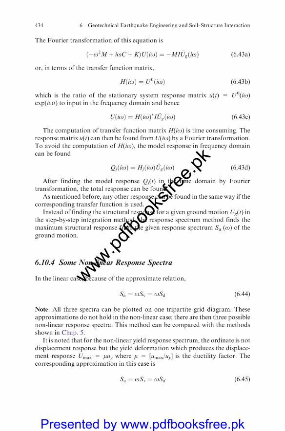
The Fourier transformation of this equation is
ð�o2Mþ ioCþ KÞUðioÞ ¼ �MI €UgðioÞ (6:43a)
or, in terms of the transfer function matrix,
HðioÞ ¼ U 0ðioÞ (6:43b)
which is the ratio of the stationary system response matrix u(t) = U 0(io)exp(iot) to input in the frequency domain and hence
UðioÞ ¼ HðioÞ�I €UgðioÞ (6:43c)
The computation of transfer function matrix H(io) is time consuming. Theresponse matrix u(t) can then be found fromU(io) by a Fourier transformation.To avoid the computation of H(io), the model response in frequency domaincan be found
QjðioÞ ¼ HjðioÞ €UgðioÞ (6:43d)
After finding the model response Qj(t) in the time domain by Fouriertransformation, the total response can be found.
As mentioned before, any other response can be found in the same way if thecorresponding transfer function is used.
Instead of finding the structural response for a given ground motionUg(t) inthe step-by-step integration method, the response spectrum method finds themaximum structural response from the given response spectrum Sa (o) of theground motion.
6.10.4 Some Non-linear Response Spectra
In the linear case, because of the approximate relation,
Sa ¼ oSv ¼ oSd (6:44)
Note: All three spectra can be plotted on one tripartite grid diagram. Theseapproximations do not hold in the non-linear case; there are then three possiblenon-linear response spectra. This method can be compared with the methodsshown in Chap. 5.
It is noted that for the non-linear yield response spectrum, the ordinate is notdisplacement response but the yield deformation which produces the displace-ment response Umax = muy where m = [umax/uy] is the ductility factor. Thecorresponding approximation in this case is
Sa ¼ oSv ¼ oSd (6:45)
434 6 Geotechnical Earthquake Engineering and Soil–Structure Interaction
www.pdfbo
oksfr
ee.pk
Presented by www.pdfbooksfree.pk
And the yield strength of the concrete structure is
Py ¼ Pmax ¼ kuy ¼ mo2uy (6:46)
In an ideal elasto-plastic system, Py is the maximum internal force elastic
limit of the deformation capacity uy which the system should have in order to
limit the spectral acceleration, velocity and displacement to not over o2uy, ouyand uy, respectively. Here uy and ductility factor It are requirements of the
capacity for the system. Finally, four structural factors (natural period, damp-
ing ratio, type of hysteretic curve and the ductility factor m) and three ground
motion parameters (peak acceleration A, velocity V and displacement D) are
obtained for analysis.
6.10.5 Soil–Structure Interaction Numerical Technique
Soil–structure interaction (SSI) was first studied a long time ago in analysis of
the vibration of machinery foundations but has developed greatly in the past
two decades because of the rapid advances in computer technology. It may be
classified into time and frequency domains in methodology or total structure
concept or substructure and hybrid structure in structural decomposition.Most
investigators have adopted frequency–domain analysis which has the following
advantages.
(a) It is convenient to consider the frequency-dependent foundation impedancewhen the whole system is divided into structure and ground.
(b) The transmitting boundary for a finite element model or wave propagationtheory is frequency dependent.
Generally speaking, SSI analysis consists of four fundamental problems as
follows:
(i) The free-field problem: the rock (ground) motion is found from other givenmotions.
(ii) The scattering problem: the response of the ground is studied with thestructure removed at the contacts (Fig. 6.6) of the structure and ground.The different contact points of the hybrid structure are studied, includingthe foundation soil and the remaining half-space.
(iii) Impedance: the displacements Uc(o) exp(iot) at the contact points arefound for forces applied at the contact point Fc(o) exp(iot). The impe-dance matrix Is(o) =C�1(o) or the flexibility matrixC(o) of the ground isdefined in the following ratio:
UcðoÞ ¼ CðoÞFcðoÞ (6:47)
6.10 Site Response 435
www.pdfbo
oksfr
ee.pk
Presented by www.pdfbooksfree.pk
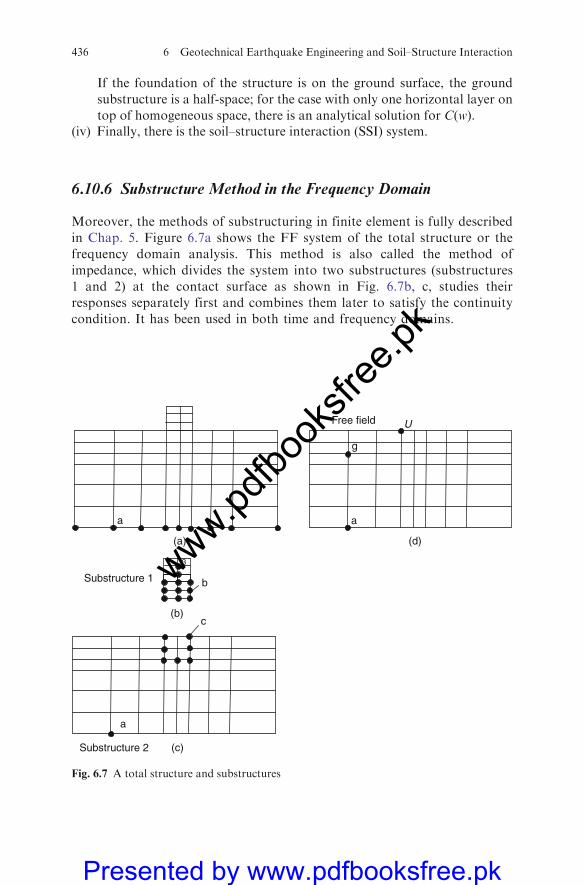
If the foundation of the structure is on the ground surface, the ground
substructure is a half-space; for the case with only one horizontal layer on
top of homogeneous space, there is an analytical solution for C(w).(iv) Finally, there is the soil–structure interaction (SSI) system.
6.10.6 Substructure Method in the Frequency Domain
Moreover, the methods of substructuring in finite element is fully described
in Chap. 5. Figure 6.7a shows the FF system of the total structure or the
frequency domain analysis. This method is also called the method of
impedance, which divides the system into two substructures (substructures
1 and 2) at the contact surface as shown in Fig. 6.7b, c, studies their
responses separately first and combines them later to satisfy the continuity
condition. It has been used in both time and frequency domains.
a
(a)
a
g
Free field
(d)
U
a
(c)Substructure 2
b
(b)
3
Substructure 1
c
Fig. 6.7 A total structure and substructures
436 6 Geotechnical Earthquake Engineering and Soil–Structure Interaction
www.pdfbo
oksfr
ee.pk
Presented by www.pdfbooksfree.pk
Let the known motion be a general three-dimensional time history ug(t),whose frequency domain expression is Ug(o) at some depth below the surface.The four primary problems are encountered:
(a) Free-field response: the input motion ua (t) orUa (o) is evaluated as bedrockpoint ‘‘a’’ in Fig. 6.8d, the lower boundary of the ground substructure forgiven motional point g. Let the analysis use Din operator L1
*:
L�1 : uaðtÞ;Ua; ðoÞ ¼ uðtÞ;U0gðoÞ (6:48)
(b) Scattering problem: the response of substructure 2 is studied(Fig. VIII.8(c)). Let there be an operator Li
*:
L�2 : u0gðtÞ;U0ðoÞ ¼ uaðtÞ;UaðoÞ (6:49)
(c) mpedance problem: the response of substructure 2 is studied (Fig. 6.8(c))under an external excitation fc(t) = Fc(o)Fc(iot) acting along one directionat any point c. The response at point c, uc(t) = Uc(o) exp (iot) for a givenforce fb(o) = Fb(o)exp(iot) at point c is
UcðoÞ ¼ CðoÞFcðoÞ FcðoÞ ¼ IsðoÞUcðoÞCðoÞ (6:50)
(d) The response ub(t) or Ub(o) of substructure 1 under external forces fb(t) =Fb (o) exp(iot) is studied at contact point b:
FbðoÞ ¼MbðoÞo2 UbðoÞ (6:51)
where Mb(o) is the equivalent, frequency-dependent mass matrix of thesuperstructure.
The four primary problems are four steps to find the operators L1*, L2*,C(o) or Is(o) andMb(o). The final solution is only an assemblage of the four tosatisfy the compatibility requirement at the boundary points b and c.
The continuity condition at boundary points b and c is that the displacementub(t) or Ub(o) is equal to the sum of displacements uc
0(t) or Uc0(o) of substruc-
ture 2 and the displacements uc(t) orUc(w) due to the SSI effect of substructure 1on substructure 2:
ubðtÞ ¼ u0cðtÞ þ ucðtÞ orbðoÞ ¼ U0cðoÞ þUcðoÞ (6:52)
The equilibrium condition requires that the sum of forces f(t) or Fc(o)between the ground and foundation and the forces fb(t) or Fb(o) between thestructure and foundation resist the inertial force fi( t) or Fi(o) of the rigidfoundation, i.e.
ubðtÞ ¼ u0cðtÞ þ ucðtÞ or FcðoÞ ¼M0 o2UbðwÞ þ FbðoÞ (6:53)
whereM0W2Ub(o) is the Fourier transform of the inertial force fi(t) andM0 the
mass matrix of the rigid foundation.
6.10 Site Response 437
www.pdfbo
oksfr
ee.pk
Presented by www.pdfbooksfree.pk
From these Fourier equations it is finally found that
UbðoÞ ¼ fI� o2CðoÞ½M0 þMbðoÞ�g�1U 0cðoÞ (6:54)
or
UbðoÞ ¼ fIsðoÞ � o2½M0 þMbðoÞ�g�1 U 0cðwÞ (6:55)
F0cðoÞ ¼ IsðoÞU0
cðoÞ (6:56)
where I is the identity matrix. If three-dimensional ground motion is consid-ered, a rigid foundation has six components: three translational and threerotational, and I is 6 � 6. Equation (6.54) clearly shows the interactions. Theeffect of input motion ug(t) is represented by Uc
0(o), the foundation inputmotion obtained by operators L1 and L2; the interaction of the superstructurefoundation and ground by the termC(o)[M0+Mb(o)] andUb(o) is the result ofthe input motion on the soil–structure system, from which the structuralresponse is obtained.
In (6.55), Fc0(o) = Is(o)Uc
0(o) is the driving force vector which includes theforces and moments from the rigid foundation on the ground when points c ofthe substructure 2 tend to deform and the foundation resists the deformation.Equations (6.55) and (6.56) are easier to use than Eq. (6.54).
6.11 Mode Superposition Method – Numerical Modelling
The alternative numerical method under mode superposition given in Chap. 5can be adopted for superstructures.
Mode superposition method is a method of using the natural frequencies andmode shapes from the modal analysis to characterize the dynamic response of astructure to transient or steady harmonic excitations.
The equations of motion may be expressed as stated before in Chap. 5:
½M�f€ug þ ½C�f€ug þ ½K�fug ¼ fFg (6:57)
{F} is the time-varying load vector given by
fFg ¼ fFndg þ sfFSg (6:58)
where {Fnd} is the time-varying nodal forces; s is the load vector scale factor and{F} is the load factor from the modal analysis.
The procedure of setting modal coordinates are clearly established as indi-cated in Chap. 5. Equation (6.57) is then reset and orthogonality conditions areestablished. Normality conditions given in (6.59) are established:
ffigIfMgffjg ¼ 1 (6:59)
438 6 Geotechnical Earthquake Engineering and Soil–Structure Interaction
www.pdfbo
oksfr
ee.pk
Presented by www.pdfbooksfree.pk
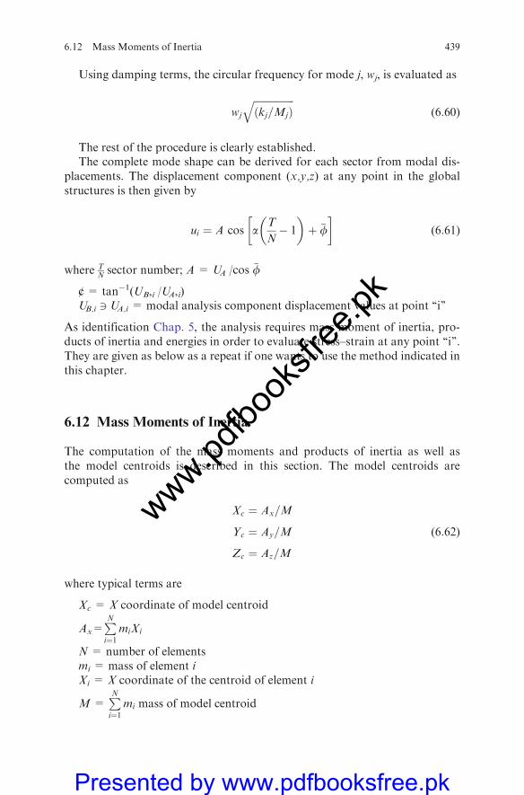
Using damping terms, the circular frequency for mode j, wj, is evaluated as
wj
ffiffiffiffiffiffiffiffiffiffiffiffiffiffiffiffiðkj=MjÞ
q(6:60)
The rest of the procedure is clearly established.The complete mode shape can be derived for each sector from modal dis-
placements. The displacement component (x,y,z) at any point in the globalstructures is then given by
ui ¼ A cos aT
N� 1
� �þ �f
� �(6:61)
where TNsector number; A = UA /cos �f
¢ = tan�1(UB,i /UA,i)UB,i 3 UA,i = modal analysis component displacement values at point ‘‘i’’
As identification Chap. 5, the analysis requires mass moment of inertia, pro-ducts of inertia and energies in order to evaluate stress–strain at any point ‘‘i’’.They are given as below as a repeat if one wants to use the method indicated inthis chapter.
6.12 Mass Moments of Inertia
The computation of the mass moments and products of inertia as well asthe model centroids is described in this section. The model centroids arecomputed as
Xc ¼ Ax=M
Yc ¼ Ay=M
Zc ¼ Az=M
(6:62)
where typical terms are
Xc = X coordinate of model centroid
Ax=PNi¼1
miXi
N = number of elementsmi = mass of element iXi = X coordinate of the centroid of element i
M =PNi¼1
mi mass of model centroid
6.12 Mass Moments of Inertia 439
www.pdfbo
oksfr
ee.pk
Presented by www.pdfbooksfree.pk
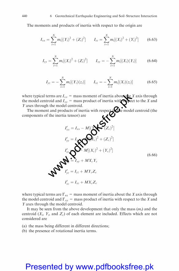
The moments and products of inertia with respect to the origin are
Ixx ¼XNi¼1
mi½ðYiÞ2 þ ðZiÞ2� Izz ¼XNi¼1
mi½ðXiÞ2 þ ðYiÞ2� (6:63)
Iyy ¼XNi¼1
mi½ðXiÞ2 þ ðZiÞ2� Ixy ¼ �XNi¼1
mi½ðXiÞðYiÞ� (6:64)
Iyz ¼ �XNi¼1
mi½ðYiÞðziÞ� Ixz ¼ �XNi¼1
mi½ðXiÞðziÞ� (6:65)
where typical terms are Ixx =mass moment of inertia about the X axis throughthe model centroid and Ixy =mass product of inertia with respect to the X andY axes through the model centroid.
The moment and products of inertia with respect to the model centroid (thecomponents of the inertia tensor) are
I 0xx ¼ Ixx �M½ðYcÞ2 þ ðZcÞ2�
I 0yy ¼ Iyy �M½ðXcÞ2 þ ðZcÞ2�
I 0zz ¼ Izz �M½ðXcÞ2 þ ðYcÞ2�
I 0xy ¼ Ixy þMXcYc
I 0yz ¼ Iyz þMYcZc
I 0xz ¼ Ixz þMXcZc
(6:66)
where typical terms are I0xx =mass moment of inertia about theX axis throughthe model centroid and I0xy =mass product of inertia with respect to the X andY axes through the model centroid.
It may be seen from the above development that only the mass (mi) and thecentroid (Xi, Yi, and Zc) of each element are included. Effects which are notconsidered are
(a) the mass being different in different directions;(b) the presence of rotational inertia terms.
440 6 Geotechnical Earthquake Engineering and Soil–Structure Interaction
www.pdfbo
oksfr
ee.pk
Presented by www.pdfbooksfree.pk
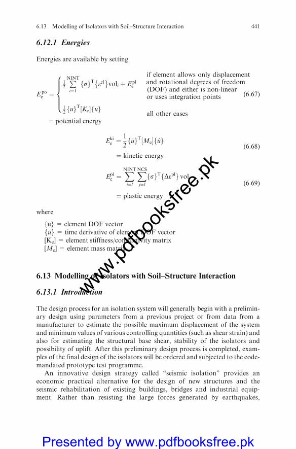
6.12.1 Energies
Energies are available by setting
E poe ¼
12
PNINT
i¼1sf gT eel
�voli þ Epl
e
12
uf gT Ke½ � uf g
8>>><>>>:
if element allows only displacementand rotational degrees of freedom(DOF) and either is non-linearor uses integration points
all other cases
(6:67)
¼ potential energy
Ekie ¼
1
2f _ugT½Me�f _ug
¼ kinetic energy
(6:68)
Eple ¼
XNINT
i¼l
XNCS
j¼lfsgTfDeplg voli
¼ plastic energy
(6:69)
where
{u} = element DOF vectorf _ug= time derivative of element DOF vector[Ke] = element stiffness/conductivity matrix[Me] = element mass matrix
6.13 Modelling of Isolators with Soil–Structure Interaction
6.13.1 Introduction
The design process for an isolation system will generally begin with a prelimin-ary design using parameters from a previous project or from data from amanufacturer to estimate the possible maximum displacement of the systemandminimum values of various controlling quantities (such as shear strain) andalso for estimating the structural base shear, stability of the isolators andpossibility of uplift. After this preliminary design process is completed, exam-ples of the final design of the isolators will be ordered and subjected to the code-mandated prototype test programme.
An innovative design strategy called ‘‘seismic isolation’’ provides aneconomic practical alternative for the design of new structures and theseismic rehabilitation of existing buildings, bridges and industrial equip-ment. Rather than resisting the large forces generated by earthquakes,
6.13 Modelling of Isolators with Soil–Structure Interaction 441
www.pdfbo
oksfr
ee.pk
Presented by www.pdfbooksfree.pk
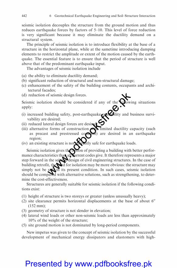
seismic isolation decouples the structure from the ground motion and thusreduces earthquake forces by factors of 5–10. This level of force reductionis very significant because it may eliminate the ductility demand on astructural system.
The principle of seismic isolation is to introduce flexibility at the base of astructure in the horizontal plane, while at the sametime introducing dampingelements to restrict the amplitude or extent of the motion caused by the earth-quake. The essential feature is to ensure that the period of structure is wellabove that of the predominant earthquake input.
The advantages of seismic isolation include
(a) the ability to eliminate ductility demand;(b) significant reduction of structural and non-structural damage;(c) enhancement of the safety of the building contents, occupants and archi-
tectural facades;(d) reduction of seismic design forces.
Seismic isolation should be considered if any of the following situationsapply:
(i) increased building safety, post-earthquake operability and business survi-vability are desired;
(ii) reduced lateral design forces are desired;(iii) alternative forms of construction with limited ductility capacity (such
as precast and prestressed concrete) are desired in an earthquakeregion;
(iv) an existing structure is not currently safe for earthquake loads.
Seismic isolation gives the option of providing a building with better perfor-mance characteristics than all current codes give. It therefore represents a majorstep forward in the seismic design of civil engineering structures. In the case ofbuilding retrofit, the need for isolation may be more obvious: the structure maysimply not be safe in its present condition. In such cases, seismic isolationshould be compared with alternative solutions, such as strengthening, to deter-mine the cost-effectiveness.
Structures are generally suitable for seismic isolation if the following condi-tions exist:
(1) height of structure is two storeys or greater (unless unusually heavy);(2) site clearance permits horizontal displacements at the base of about 600
(152 mm);(3) geometry of structure is not slender in elevation;(4) lateral wind loads or other non-seismic loads are less than approximately
10% of the weight of the structure;(5) site ground motion is not dominated by long-period components.
New impetus was given to the concept of seismic isolation by the successfuldevelopment of mechanical energy dissipators and elastomers with high-
442 6 Geotechnical Earthquake Engineering and Soil–Structure Interaction
www.pdfbo
oksfr
ee.pk
Presented by www.pdfbooksfree.pk
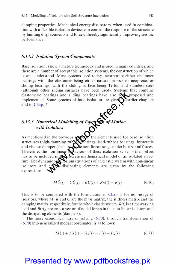
damping properties. Mechanical energy dissipators, when used in combina-tion with a flexible isolation device, can control the response of the structureby limiting displacements and forces, thereby significantly improving seismicperformance.
6.13.2 Isolation System Components
Base isolation is now a mature technology and is used in many countries, andthere are a number of acceptable isolation systems, the construction of whichis well understood. Most systems used today incorporate either elastomerbearings with the elastomer being either natural rubber or neoprene, orsliding bearings, with the sliding surface being Teflon and stainless steel(although other sliding surfaces have been used). Systems that combineelastomeric bearings and sliding bearings have also been proposed andimplemented. Some systems of base isolation are given in earlier chaptersand in Chap. 5.
6.13.3 Numerical Modelling of Equations of Motionwith Isolators
As mentioned in the previous sections, the elements used for base isolationstructures (high-damping rubber bearings, lead-rubber bearings, hystereticand viscous dampers) behave in the non-linear range under horizontal forces.Therefore, the non-linear behaviour of these isolation systems themselveshas to be included in the discrete mathematical model of an isolated struc-ture. The dynamic equilibrium equations of an elastic system with non-linearisolators and energy-dissipating elements are given by the followingexpression:
M €UðtÞ þ C _UðtÞ þ KUðtÞ þ RNðtÞ ¼ RðtÞ (6:70)
This is to be compared with the formulation in Chap. 5 for non-usage ofisolators, where M, K and C are the mass matrix, the stiffness matrix and thedampingmatrix, respectively, for the whole elastic system.R(t) is a time-varyingload and R(t)N presents a vector of nodal forces in the non-linear isolators andthe dissipating elements (dampers).
The more economical way of solving (6.70), through transformation of(6.70) into generalized modal coordinates, is as follows:
IXðtÞ þ LXðtÞ ¼ OXðtÞ ¼ FðtÞ � FNðtÞ (6:71)
6.13 Modelling of Isolators with Soil–Structure Interaction 443
www.pdfbo
oksfr
ee.pk
Presented by www.pdfbooksfree.pk
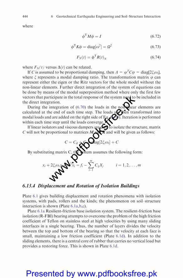
where
fTMf ¼ I (6:72)
fTKf ¼ diag½o2� ¼ O2 (6:73)
FNðtÞ ¼ fTRðtÞN (6:74)
where FN(t) versus DðtÞ can be related.If C is assumed to be proportional damping, then L= jTCj= diag[2xioi],
where x represents a modal damping ratio. The transformation matrix j canrepresent either the eigen or the Ritz vectors for the whole model without thenon-linear elements. Further direct integration of the system of equations canbe done by means of the modal superposition method where only the first fewvectors that participate in the total response of the system need to be included inthe direct integration.
During the integration of (6.70) the loads in the non-linear elements arecalculated at the end of each time step. The loads are then transformed intomodal loads and are added on the right side of Eq. (6.70). Iteration is performedwithin each time step until the loads converge.
If linear isolators and viscous dampers are used to isolate the structure, matrixC will not be proportional to matricesM and K and will be given as follows:
C ¼ Cd þ C ¼ diag½2xioi� þ C
By substituting matrix C, the system assumes the following form:
xi þ 2xioixþ o2xi ¼ fi �Xmi�1
CijXj i ¼ 1; 2; . . . ;m
6.13.4 Displacement and Rotation of Isolation Buildings
Plate 6.1 gives building displacement and rotation phenomena with isolationsystems, with pads, rollers and the kinds; the phenomenon on soil–structureinteraction is shown (Plate 6.1a,b,c).
Plate 6.1a Resilient-friction base isolation system. The resilient-friction baseisolation (R-FBI) bearing attempts to overcome the problem of the high frictioncoefficient of Teflon on stainless steel at high velocities by using many slidinginterfaces in a single bearing. Thus, the number of layers divides the velocitybetween the top and bottom of the bearing so that the velocity at each face issmall, maintaining a low friction coefficient (Plate 6.1d). In addition to thesliding elements, there is a central core of rubber that carries no vertical load butprovides a restoring force. This is shown in Plate 6.1d.
444 6 Geotechnical Earthquake Engineering and Soil–Structure Interaction
www.pdfbo
oksfr
ee.pk
Presented by www.pdfbooksfree.pk
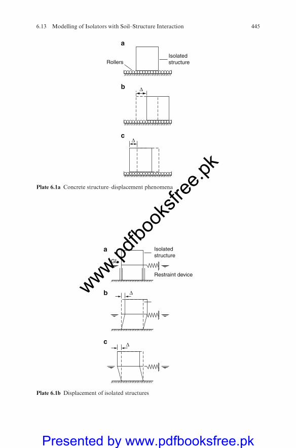
Isolatedstructure
Restraint device
GL
Δ
Δ
a
b
c
Plate 6.1b Displacement of isolated structures
Isolatedstructure
Δ
Δ
Rollers
a
b
c
Plate 6.1a Concrete structure–displacement phenomena
6.13 Modelling of Isolators with Soil–Structure Interaction 445
www.pdfbo
oksfr
ee.pk
Presented by www.pdfbooksfree.pk

6.13.4.1 Reactor Containment Building
The actual cross-section of the TVA prestressed concrete containment building
is given in Figs. 6.8 and 6.9. The finite element model is given in Fig. 6.10 usingsoil-structure interaction concept described in this chapter using the kobeearthquake in Japan; the complete deformed containment building with cracks
in concrete and complete failure of prestressing tendons is shown in Fig. 6.11.This is the damage model for the Kobe earthquake of frequency 8.5–9.5 Hz.
GapRubber plug
Rubber plug
Rubber core
Sliding platesTeflon layers
Bottom plate
Top connecting plate
Central steel rodPlate 6.1d Isolators withlow friction
Isolatedstructure
Δ
Δ
a
b
c
Plate 6.1c Displacementand rotation of concretestructures
446 6 Geotechnical Earthquake Engineering and Soil–Structure Interaction
www.pdfbo
oksfr
ee.pk
Presented by www.pdfbooksfree.pk

EL 259.9
EL 259.6const JT
const JT
const JT
const JT
const JTconst JT
EL 260.8
EL 261.2EL 262.45EL 263.0EL 260.6
EL 264.9
EL 265.66
EL 266.4
1.678 m
457 mm
springline
6 mm A liner(typical)
533 mmvertical tendons
3.06 m
El 189.71.22 m
0.61
EL 187.1
0.763533 mm
EL 185
coupling device
EL 184.5
2.44 m
0.763EL 187.6
EL 189.1
secondarycontainment
vertical angles (typ)
horizontal channels (typ)
horiz
onta
l (ho
op)
tend
ons
0.76
3
1.14 EL 186.8
EL 258.9
true elliptical curve(major axis = 41.175 m)(minor axis = 24.248 m)
tendon layers ‘A’ & ‘C’ arerotated in this section inorder to clarify theirposition in their vertical plane
const JT229 mm
0.915 m
35.9˚
8˚
CL layer ‘A’CL layer ‘B’
CL layer ‘C’
1.53 m
1.53 m
Fig. 6.8 Typical section – wall and dome (courtesy of TVA and Bellefonte NPS)
6.13 Modelling of Isolators with Soil–Structure Interaction 447
www.pdfbo
oksfr
ee.pk
Presented by www.pdfbooksfree.pk
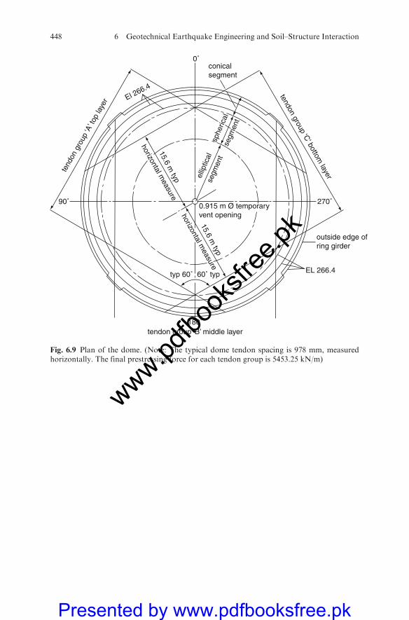
270˚
EL 266.4typ 60˚
180˚tendon group ‘B’ middle layer
60˚ typ
15.6 m typ
15.6 m typ
horizontal measure
horizontal measure
tendon group ‘C’ bottom
layer
tend
on g
roup
‘A’ t
op la
yer
outside edge ofring girder
0.915 m Ø temporaryvent opening
0˚
90˚
conicalsegment
El 266.4
ellip
tical
segm
ent
sphe
rical
segm
ent
Fig. 6.9 Plan of the dome. (Note: The typical dome tendon spacing is 978 mm, measuredhorizontally. The final prestressing force for each tendon group is 5453.25 kN/m)
448 6 Geotechnical Earthquake Engineering and Soil–Structure Interaction
www.pdfbo
oksfr
ee.pk
Presented by www.pdfbooksfree.pk
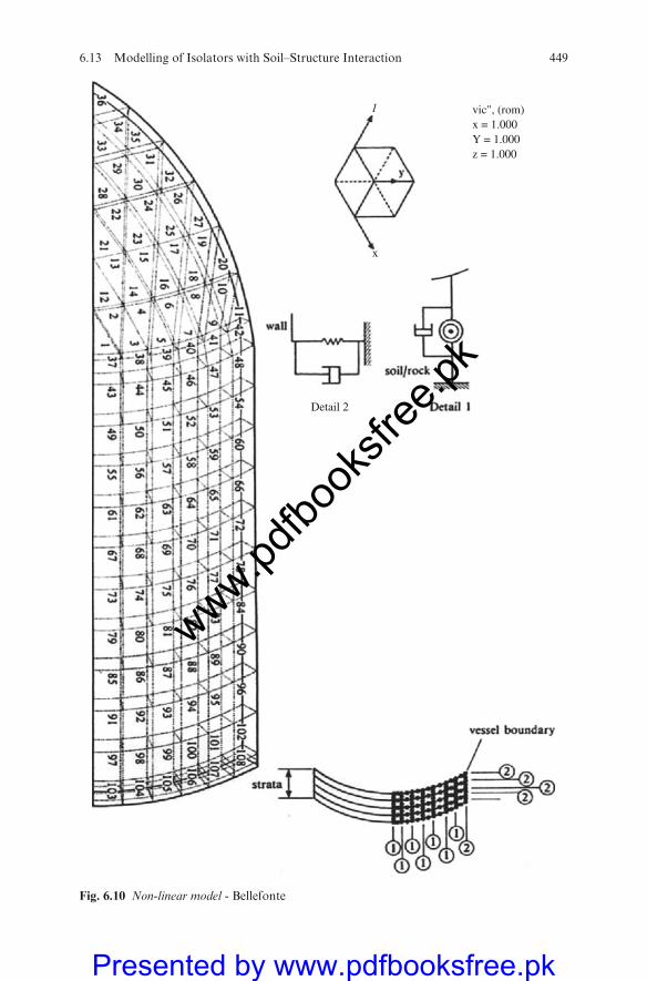
1 vic", (rom) x = 1.000 Y = 1.000 z = 1.000
x
Detail 2
Fig. 6.10 Non-linear model - Bellefonte
6.13 Modelling of Isolators with Soil–Structure Interaction 449
www.pdfbo
oksfr
ee.pk
Presented by www.pdfbooksfree.pk
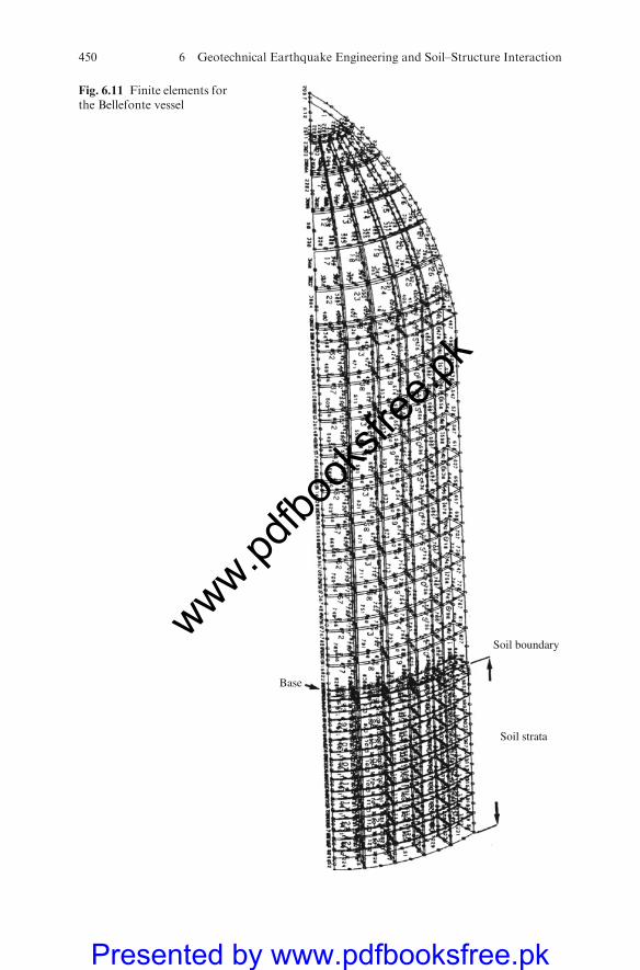
Soil boundary
Soil strata
Base
Fig. 6.11 Finite elements forthe Bellefonte vessel
450 6 Geotechnical Earthquake Engineering and Soil–Structure Interaction
www.pdfbo
oksfr
ee.pk
Presented by www.pdfbooksfree.pk
for containment vessels subjected to internal pressures up to 344.75 kN/m2
along with dead, live and prestressing loads. The idealized strata in case of
the Bellefonte vessel are given in Fig. 6.11 for the vessel parameters shown in
Figs. 6.9 and 6.10.(i) Missile loads (Ym). In nuclear plant design, components and equipment should
be protected against loss of function due to plant-generated and extreme environ-
mental missile.Where a containment building is close to amajor airport the damage
caused by a otential missile such as an aircraft crash should be considered.
Bibliography
Akiyama, H. Earthquake Resistant Limit-State Design for Buildings. University of TokyoPress, Tokyo, Japan, 1985.
Bendat, J. S. and Piersol, A. G. Random Data: Analysis and Measurement Procedures. JohnWiley and Sons, Inc., New York, 1971.
Berg, G. V. and Thomaides, T. T. Energy consumption by structures in strong-motion earth-quakes. Proc. 2nd World Conf. Earthquake Eng., Tokyo and Kyoto, 1960; pp. 681–696.
Blackman, R. and Tuckey, J. W. TheMeasurement of Power Spectra from the Point of View ofCommunication Engineering. Dover Publications, New York, 1959.
Caughey, T. K. and Stumpf, H. J. Transient response of a dynamic system under randomexcitation. J. Appl. Mech. 1961; 28:563–566.
Chaboche, L. J. Constitutive equation for cyclic plasticity and cyclic viscoplasticity. Int. J.Plasticity 1989; 5:247–301.
Clough, R. W. Analysis of structural vibrations and dynamic response. Proc. 1st US-JapanSymp. Recent Adv. Matrix Meth. Struct. Anal. Design, Tokyo (1969), University ofAlabama Press, 1971.
Corotis, R. B. Time-dependent power spectra and first passage probabilities. MIT Civil Engi-neering Research Report R7D-78, Massachusetts Institute of Technology, Cambridge,MA, 1970.
Corotis, R. B., Vanmarcke, E. H., and Cornell, C. A. First passage of nonstationary randomprocesses. J. Eng. Mech. Div.(ASCE) 1972; 98:401–414.
Craig, R. and Bampton, M. Coupling of structures for dynamic analysis. AIAA J. 1968;6:1313–1319.
Fajfar, P. and Vidic, T. Consistent inelastic design spectra: hysteretic and input energy.Earthquake Eng. Struct. Dyn. 1994; 23:523–537.
Goel, S. C. and Berg, G. V. Inelastic earthquake response of tall steel frames. J. Struct. Div.(ASCE) 1968; 94:1907–1934.
Housner, G. W. Limit design of structures to resist earthquakes. Proc. First World Conf.Earthquake Eng., Berkeley, CA, 1956; Vol. 5, pp. 1–11.
Housner, G. W. Behavior of structures during earthquakes. J. Eng. Mech. Div.(ASCE) 1959;85(4):109–129.
Housner, G. W. and Jennings, P. C. The capacity of extreme earthquake motions to damagestructures. Structural and Geotechnical Mechanics: A volume honoring NM Newmark(Hall, W. J., ed.). Prentice-Hall, Englewood Cliff, NJ, 1975; pp. 102–116.
Japan Road Association. Design Specification for Highway Bridges, Part V (Seismic Design).Maruzen Press, Tokyo, 1998.
Kato, B. and Akiyama, H. Energy input and damages in structures subjected to severeearthquakes. J. Struct. Const. Eng.(AU) 1975; 235:9–18 (in Japanese).
Kausch, H. H. Polymer Fracture (2nd revised edn). Springer-Verlag, Berlin, 1987.
Bibliography 451
www.pdfbo
oksfr
ee.pk
Presented by www.pdfbooksfree.pk
Kausel, E., Roesset, J. M., and Waas, G. Dynamic analysis of footings on layered media.J. Eng. Mech. Div. (ASCE) 1975; 101:679–693.
Kuwamura, H., Kirino, Y., and Akiyama, H. Prediction of earthquake energy input fromsmoothed Fourier amplitude spectrum.Earthquake Eng. Struct. Dyn. 1994; 23: 1125–1137.
Lee, T. H. andWesley, D. A. Soil-structure interaction of nuclear reactor structures consider-ing through-soil coupling between adjacent structures. Nucl. Eng. Design 1973; 24:374–387.
Leger, P. and Dussault, S. Seismic-energy dissipation in MDOF structures. J. Struct. Eng.(ASCE) 1992; 118(5):1251–1269.
Lewangamage, C. S.Measurement of strain field of continua by image analysis and its applica-tion to understanding behavior of rubber. Master Thesis, The University of Tokyo, Japan,2001.
Lewangamage, C. S., Abe, M., Fujino, Y., and Yoshida, J. Characteristics of rubber used inseismic isolation by digital and thermal image analysis. Proc. 9th Int. Symp. Smart Struct.Mater., San Diego, USA, 2002; Vol. 9.
Luco, E., Hadjian, A. H., and Bos, H. D. The dynamic modeling of the half-plane by finiteelements. Nucl. Eng. Design 1974; 31:184–194.
Luco, J. E. Torsional response of structures to obliquely incident seismic SH waves. Int. J.Earthquake Eng. Struct. Dyn. 1976; 4:207–219.
Lyon, R. H. Statistical Energy Analysis of Dynamical Systems. MIT Press, Cambridge, MA,1975.
Lysmer, J. and Richart, F. E. Dynamic response of footings to vertical loading. J. Soil Mech.Found. Div. (ASCE) 1966; 92(SM1):65–91.
Mahin, S. A. and Lin, J. Construction of inelastic response spectrum for single-degree-of-freedom system. Report No. UCB/EERC-83/17, Earthquake Engineering ResearchCenter, University of California, Berkeley, CA, 1983.
Mori, A., Carr, A. J., Cooke, N., and Moss, P. I. Compression behaviour of bridge bearingsused for seismic isolation. Eng. Struct. 1996; 18(5):351–362.
Ogawa, K., Inoue, K., Nakashima, M. A study on earthquake input energy causing damagesin structures. J. Struct. Construct. Eng. (AU) 2000; 530:177–184 (in Japanese).
Ohi, K., Takanashi, K., and Tanaka, H. A simple method to estimate the statistical para-meters of energy input to structures during earthquakes. J. Struct. Const. Eng. (All) 1985;347:47–55 (in Japanese).
Ordaz, M., Huerta, B., and Reinoso, E. Exact computation of input-energy spectra fromFourier amplitude spectra. Earthquake Eng. Struct. Dyn. 2003; 32:597–605.
Page, C. H. Instantaneous power spectra. J. Appl. Phys. 1952; 23(I):103–106.Parmelee, R. A., Perelman, D. S., Lee, S. L., and Keer, L. M. Seismic response of structure-
foundation systems. J. Eng. Mech. Div. (ASCE) 1968; 94:1295–1315.Press, W. H., Flannery, B. P., Teukolsky, S. A., Vetterling, W. T. Numerical Recipes in
C. Cambridge University Press, Cambridge, 1988.Rejcba, C. Design of elastomer bearings. PCI J. 1964; 9:62–78.Richardson, J. D. Forced vibrations of rigid bodies on a semi-infinite elastic medium. Ph.D.
Dissertation, Nottingham University, England, 1969.Richart, F. E., Woods, R. D., and Hall, J. R. Vibration of Soils and Foundations. Prentice-
Hall, Englewood Cliffs, NJ, 1970.Riddell, R. and Garcia, J. E. Hysteretic energy spectrum and damage control. Earthquake
Eng. Struct. Dyn. 2001; 30:1791–1816.Scanlan, R. H. Seismic wave effects on soil-structure interaction. Int. J. Earthquake Eng.
Struct. Dyn. 1976; 4:379–388.Scanlan, R. H. and Sachs, K. Earthquake time histories and response spectra. J. Eng. Mech.
Div.(ASCE) 1974; 100:635–655.Shinozuka, M. Maximum structural response to seismic excitations. J. Eng. Mech. Div.
(ASCE) 1970; 96(EM5):729–738.
452 6 Geotechnical Earthquake Engineering and Soil–Structure Interaction
www.pdfbo
oksfr
ee.pk
Presented by www.pdfbooksfree.pk

Stallybrass, M. P. A variational approach to a class of mixed boundary-value problems in theforced oscillations of an elastic medium. Proc. 4th USNat. Cong. Appl. Mech. 1962; 391–400.
Takewaki, I. Optimal damper placement for minimum transfer functions. Earthquake Eng.Struct. Dyn. 1997; 26:1113–1124.
Takewaki, I. Probabilistic critical excitation for MDOF elastic-plastic structures on compli-ant ground. Earthquake Eng. Struct. Dyn. 2001a; 30:1345–1360.
Takewaki, I. A new method for non-stationary random critical excitation. Earthquake Eng.Struct. Dyn. 2001b; 30:519–535.
Takewaki, I. Critical excitation method for robust design: a review. J. Struct. Eng.(ASCE)2002a; 128(5):665–672.
Takewaki, I. Robust building stiffness design for variable critical excitations. J. Struct. Eng.(ASCE) 2002b; 128(12):1565–1574.
Takizawa, H. Energy-response spectrum of earthquake ground motions. Proc. 14th Nat.Disaster Sci. Symp., 1977; pp. 359–362, Hokkaido (in Japanese).
Tanabashi, R. Personal view on destructiveness of earthquake ground motions and buildingseismic resistance. J Architect. Buil. Sci. (AB) 1935; 48:599 (in Japanese).
Tanabashi, R. Studies on the nonlinear vibrations of structures subjected to destructiveearthquakes. Proc. First World Conf. Earthquake Eng., Berkeley, CA, 1956; Vol. 6,pp. 1–16.
Treloar, L. R. G. The Physics of Rubber Elasticity (3rd edn). Clarendon Press, Oxford, 1975.Uang, C. M. and Bertero, V. V. Evaluation of seismic energy in structures. Earthquake Eng.
Struct. Dyn. 1990; 19:77–90.Uchida, K., Miyashita, T., and Nagata, S. Earthquake response analysis of a nuclear power
plant reactor building with a circular base mat. Annual Report of the Kajima Institute ofConstruction Technology, 21, 98–99, first published in Japanese in June 1973.
Veletsos, A. S. and Ventura, C. E. O. Modal analysis of non-classically damped linearsystems. Earthquake Eng. Struct. Dyn. 1986; 14:217–243.
Veletsos, A. S. andWei, Y. T. Lateral and rocking vibration of footings. J. Soil Mech. Found.Div. (ASCE) 1971; 97:1227–1248.
Yamashita, Y., Kawabata, S. Strain energy density approximation formula for carbon-filledrubber. Jpn. Rubber Assoc. 1992; 65:517–527 (in Japanese).
Zahrah, T. F. and Hall, W. J. Earthquake energy absorption in SDOF structures. J. Struct.Eng.(ASCE) 1984; 110(8):1757–1772.
Bibliography 453
www.pdfbo
oksfr
ee.pk
Presented by www.pdfbooksfree.pk

www.pdfbo
oksfr
ee.pk
Presented by www.pdfbooksfree.pk
Chapter 7
Response of Controlled Buildings – Case Studies
7.1 Introduction
This chapter deals with a number of buildings constructed with differentmaterials, vertical and plain dimensions and variable floor areas. The heightof a building is measured to its eaves level. The classification of buildingstructure can be identified as made up of reinforced concrete with or withoutprestressing elements, structural steel, steel–concrete composite and manyothers in combination. The building can be built as three-dimensionalmoment frame with shear walls with individual spread footings or mat systemsand RC/steel pile foundation. The building cited on site may have a differentfoundation or ground properties. Where ground properties are unknown, theanalysis for soil structure interaction is based on Chap. 6 and Chap. 7, as perdetails given in Table 7.1. Various devices for the buildings have beendescribed in this text and they have been used to make the building ascontrolled structures. For checking various buildings irrespective of how tallthey are, the devices such as isolators, dampers contribute to control accel-eration, displacement, velocity and the total drift. A comparative study ismade between the designer’s results and results produced by the author. Inmany areas the collaboration is excellent between the results given by theoriginal designers and those evaluated by the author using three differentcomputer packages, namely, programs ISOPAR, ETAB and SAP2000.Some results are presented in graphical form and some are compared intabulated form as a comparative study of individual test cases for variousconstructed facilities. Seismic waveforms such as El-Centro NS and Taft EWhave been adopted for cases where the information was not available. In somecases the waveform for Kobe earthquake has been used to evaluate variousparameters. The reader has a choice to adopt any specific waveform forbuilding in seismic area where information cannot, for some reason, beobtained.
The author has analysed quite a few buildings of constructed facilities ascontrolled structures and related their displacement, velocities and accelera-tion to the height and total floor areas. The obvious problems are theintricate layouts of buildings and the relevant positioning of devices and
M.Y.H. Bangash, Earthquake Resistant Buildings,DOI 10.1007/978-3-540-93818-7_7, � M.Y.H. Bangash 2011
455
www.pdfbo
oksfr
ee.pk
Presented by www.pdfbooksfree.pk
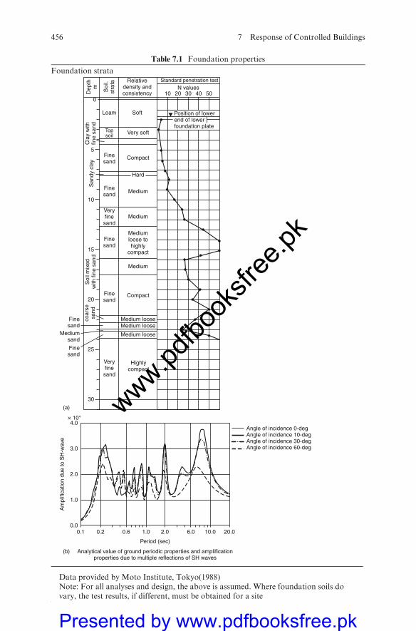
Table 7.1 Foundation properties
Foundation strata
Dep
thm Soi
l.st
rata Relative
density andconsistency
Soft Position of lowerend of lowerfoundation plate
Loam
0
5
10
15
20
25
30
4.0× 10°
3.0
2.0
Am
plifi
catio
n du
e to
SH
-wav
e
1.0
0.00.1 0.2 0.6 1.0
Period (sec)
Analytical value of ground periodic properties and amplificationproperties due to multiple reflections of SH waves
2.0 6.0 10.0 20.0
Angle of incidence 0-degAngle of incidence 10-degAngle of incidence 30-degAngle of incidence 60-deg
(a)
(b)
Topsoil
Cla
y w
ithfin
e sa
ndS
andy
cla
y
Finesand
Finesand
Veryfine
sand
Finesand
Finesand
Soi
l mix
edw
ith fi
ne s
and
coar
sesa
nd
Finesand
Finesand
Mediumsand
Veryfine
sand
Highlycompact
Medium loose
Medium looseMedium loose
Compact
Medium
Mediumloose tohighly
compact
Medium
Medium
Hard
Compact
Very soft
Standard penetration test
N values10 20 30 40 50
Data provided by Moto Institute, Tokyo(1988)Note: For all analyses and design, the above is assumed. Where foundation soils dovary, the test results, if different, must be obtained for a site
456 7 Response of Controlled Buildings
www.pdfbo
oksfr
ee.pk
Presented by www.pdfbooksfree.pk
their quantities. What the author has done is to reanalyse the existing con-structed facilities with and without devices. Displacement, velocities, accel-eration and storey drift were examined. If they are excessive without devicesbased on codified methods and practical limitations imposed, a simplenumerical relation will give the number of devices needed to control thebuilding. A random permutation and combination approach has beenadopted. This random method of algebra would decide and confirm theinitial numberof devices needed to make the building stand up to specificseismic waveform, with reduced displacements and accelerations of floorsand foundation levels. The reduction of storey drift will then confirm theanalysis to an acceptable level. It is envisaged that calculated initial numbersof devices may be lightly more or less depending upon the geometric loca-tions available in the overall layout. The author has noted that in suchcircumstances, the final prepared controlled structure has to be reanalysedusing specific analysis. In many cases, the author has used dynamic non-linear time integration approach to reanalyse the building structure. Thereanalysis will confirm whether or not its results will comply with the codelimitations. At the reanalysis stage, the number of constructed facilities waschecked again for displacement, velocity and acceleration and storey driftwith known seismic devices at each floor level where such devices could alsoeasily be accommodated. The net results are within 10% accuracy whenauthor’s results were compared with those of the designers of the existingfacilities. The results are summarized for each building of constructed facilityin the form of data, tables and graphs.
7.2 Building With Controlled Devices
Examples of response-controlled structures found in various countries areknown. The Japanese ones are first in parts (A) and (B) and Table 7.1 and part(C) to (H). The listing is just few types known to the author;
(A)1. Buildings with laminated rubber support2. Buildings with sliding supports3. Buildings with sway-type hinged columns4. Buildings with double columns5. Buildings with dampers (viscoelastic, friction)6. Buildings with dynamic dampers7. Buildings with sloshing-type dampers
7.2 Building With Controlled Devices 457
www.pdfbo
oksfr
ee.pk
Presented by www.pdfbooksfree.pk

(B) Building (Data provided by various companies) Type1. Yachiyodai Unitika Menshin Laminated rubber2. Okumura Group, Namba Research Center, office
wingLaminated rubber
3. Obayashi Group, Technical Research Center, 61Laboratory
Laminated rubber
4. Oires Industries, Fujizawa plant, TC Wing Laminated rubber5. Takenaka Komuten Funabashi Laminated
Taketomo DormitoryLaminated rubber
6. Kajima Constructions, Technical Research CenterNishi Chofu Acoustic Laboratory
Laminated rubber
7. Christian Data Bank Laminated rubber8. Tohoku University, Menshin Building Laminated rubber9. Fujita Industries, Technical Research Laboratory,
6th LaboratoryLaminated rubber
10. Shibuya Shimizu No. 1 Building Laminated rubber11. Fukumiya Apartments Laminated rubber12. Shimizu Construction, Suchiura Branch Laminated rubber13. Toranomon San-Chome Building Laminated rubber14. Department of Science and Technology, Inorganic
Material Laboratory, Vibration –free WingLaminated rubber
15. A Certain Radar Sliding support16. Taisei Construction Technical Research Center,
J WingSliding support
17. Chamber of Commerce and Culture Friction damper18. Chib Port Tower Dynamic damper19. Toyana Park Observatory Dynamic damper20. Gold Tower Sloshing damper21. Yokohama Marine Tower Sloshing damper
A typical two-storey building in Japan with devices located (Plate 7.1) will be
tested against the random method of algebra approach.
(C) Buildings with laminated rubber support (menshin structure)Structures using laminated rubber support in their foundations are the
most popular type of response-controlled structures found within and
outside Japan. It is common to use laminated rubber along with other
types of dampers. Laminated rubber is used to extend the fundamental
period of a building in the horizontal direction so that the seismic
input is reduced while the dampers absorb the incident seismic energy.
Sometimes, laminated rubber is also used to reduce the vertical
microseisms.
458 7 Response of Controlled Buildings
www.pdfbo
oksfr
ee.pk
Presented by www.pdfbooksfree.pk

Regarding building size, buildings in the USA are constructed mostly of
steel while in Japan one finds RCC structure with four to five stories. There
is also one example of a 14-storied RCC structure.(D) Buildings with sliding support
Sliding-support structures are generally used for computer room floors.
Examples using sliding supports for the entire building are very few and
only recent. This type of structure is not able to return to its original
position. When using sliding supports the position of a building after an
earthquake will be different from the one before the earthquake.(E) Buildings with double columns
Columns of low stiffness are provided in the foundation of a building. The
basic considerations are the same as those for the laminated rubber sup-
port. There are few examples of this technique, one inNewZealand and one
in Japan (Tokyo Science University).(F) Buildings with dampers (viscoelastic, friction)
Various types of dampers are installed in a multistoried structure, thus
absorbing the incident seismic energy. In the USA, buildings using viscoe-
lastic dampers (VEM) have been in use for some time to reduce the response
to strong winds. In Japan, steel dampers and friction dampers are used in
multistoried buildings.(G) Buildings with dynamic dampers
Dynamic dampers convert the vibration energy of an earthquake or wind
into kinetic energy allowing the dynamic damper to absorb the input energy.
It is used to reduce the vibrations of machinery. In the USA this technique is
mainly used to reduce the deformation of a building due to wind, while in
Japan, it is used to absorb the wind as well as earthquake energy. In Japan,
this technique is used for tower-type structures of lesser mass.(H) Buildings with sloshing-Type dampers
The incident vibration energy is absorbed as the kinetic energy of water (or
fluid) using the phenomenon of sloshing of liquids. In Japan, this technique
is mainly used for tower-type structures to reduce building deformation
due to wind or earthquake.
7.2.1 Special Symbols with Controlled Devices
Plate No. 7.1 briefly gives the symbols adopted for some devices.
7.2 Building With Controlled Devices 459
www.pdfbo
oksfr
ee.pk
Presented by www.pdfbooksfree.pk
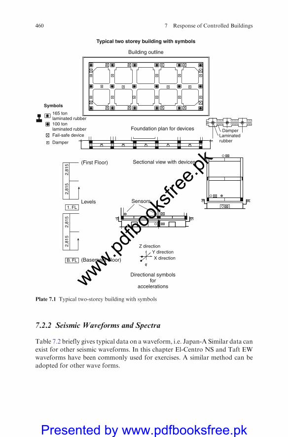
7.2.2 Seismic Waveforms and Spectra
Table 7.2 briefly gives typical data on a waveform, i.e. Japan-A Similar data can
exist for other seismic waveforms. In this chapter El-Centro NS and Taft EW
waveforms have been commonly used for exercises. A similar method can be
adopted for other wave forms.
Sectional view with devices
Levels
(First Floor)
(Basement Floor)
Sensors
Foundation plan for devices
Building outline
Typical two storey building with symbols
DamperLaminatedrubber
100 tonlaminated rubber
Symbols
Fail-safe device
Damper
165 tonlaminated rubber
1. FL
B. FL
2,81
52,
815
2,81
52,
815
Directional symbolsfor
accelerations
X direction
Z directionY direction
Plate 7.1 Typical two-storey building with symbols
460 7 Response of Controlled Buildings
www.pdfbo
oksfr
ee.pk
Presented by www.pdfbooksfree.pk
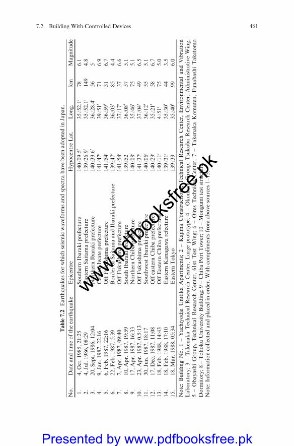
Table7.2
Earthquakes
forwhichseismicwaveform
sandspectrahavebeenadoptedin
Japan.
No.
Date
andtimeoftheearthquake
Epicentre
HypocentreLat.
Long.
km
Magnitude
1.
4,Oct.1985,21:25
SouthernIbarakiprefecture
140ff09.50
35ff52.10
78
6.1
2.
4,Jul.1986,08:29
EasternSaitamaprefecture
139ff26.90
35ff52.10
149
4.8
3.
20,Sept.1986,12:04
NorthernIbarakiprefecture
140ff39.60
36ff28.40
56
54.
9,Jan.1987,22.16
CentralIw
ate
prefecture
141ff470
39ff510
71
6.9
5.
6,Feb.1987,22:16
OffFukushim
aprefecture
141ff540
36ff590
31
6.7
6.
22,Feb.1987,5:39
Border
ofSaitamaandIbarakiprefecture
139ff470
36ff030
85
4.4
7.
7,Apr.1987,09:40
OffFukushim
aprefecture
141ff540
37ff170
37
6.6
8.
10,Apr.1987,19:59
South
Ibarakiprefecture
139ff52
36ff080
57
5.1
9.
17,Apr.1987,16:33
NorthernChibaprefecture
140ff080
35ff460
75
5.1
10.
23,Apr.1987,0.5:13
OffFukushim
aprefecture
141ff370
37ff040
49
6.5
11.
30,Jun.1987,18:17
SouthwestIbarakiprefecture
140ff060
36ff120
55
5.1
12.
17,Dec.1987,11:08
OffeasternChibaprefecture
140ff290
35ff210
58
6.7
13.
18,Feb.1988,14:43
OffEasternChibaprefecture
140ff110
4ff510
75
5.0
14.
18,Feb.1988,17:10
EasternKanagawarefecture
139ff310
35ff300
44
3.5
15.
18,Mar.1988,05:34
EasternTokyo
139ff39
35ff400
99
6.0
Note:BuildingNo.1–YachiyodaiUnitikaApartments;2–KajimaConstructions,
TechnicalResearchCenter,
EnvironmentalandVibration
Laboratory;3–TakenakaTechnicalResearchCenter,
Largeprototype;
4–Okumura
Group,TsukubaResearchCenter,
AdministrativeWing;
5–ObayashiGroup,TechnicalResearchCenter,
61st
TestWing;6–Oires
TechnicalCenter;
7–TakenakaKomuten,FunabashiTaketomo
Dorm
itory;8–TohokuUniversity
Building;9–ChibaPortTower;10–Mongumiteststructure.
Note:Inform
ationcollectedandplacedin
order.Withcomplimentsfrom
abovesources
1–15.
7.2 Building With Controlled Devices 461
www.pdfbo
oksfr
ee.pk
Presented by www.pdfbooksfree.pk
7.2.3 Maximum Acceleration and Magnification
Again eight buildings were chosen by the Japanese companies to evaluate andcompare the maximum acceleration and magnification at various floor levels ofthese buildings from basement level to the roof level. These figures are given inTable 7.3.
7.2.4 Three-Dimensional Simulation of the Seismic Wave Field
In regions such as Japan, there is a strong interaction between the details of theseismic force and the three-dimensional building structure, particularly withthe presence of subduction zones. Wherever possible modelling of the wavefield in three dimensions can then provide a useful means of simulating thelikely effect of major earthquakes. Subduction along the Nankai trough isresponsible for very large earthquakes, such as a magnitude 8.0 event. In thethree-dimensional analysis using non-linear time integration approach, ahybrid pseudo-spectral/finite element approach is used for the region. Assumethe region is 820� 410 km in horizontal dimensions and 125 km in depth. Themesh of optimum nature is 512 � 256 � 160 points with a horizontal meshincrement of 1.6 km and a vertical increment of 0.8 km can be adopted. Theminimum S-wave velocity for the superficial layer in the three-dimensionalmould is 3 km/s. The P-wave front is an outer rampart to the larger ‘S’disturbance. A reference is made to Table 7.1 for layer positioning
In some cases accurate wave fields have been correctly evaluated. Thenumerical values of accelerations for case studies have been stated. In the55-storey building, the seismic wave field mesh scheme interacts with suitablefinite element gap between the building and the foundation strata.
7.3 Evaluation of Control Devices and the Response-Control
Technique
7.3.1 Initial Statistical Investigation of Response-ControlledBuildings
The response-control technique restricts or controls the response of buildings toexternal vibrations. The responses to be restricted or controlled are accelera-tion, velocity and displacement. It is possible to control or restrict the stressesdeveloped in structural material by controlling the above responses.
The extent of restriction or control of response of buildings to external forcesusing response-control techniques can be set at any level, unlike in earlier wind-and earthquake-resistant structural methods. As a result, the response-control
462 7 Response of Controlled Buildings
www.pdfbo
oksfr
ee.pk
Presented by www.pdfbooksfree.pk
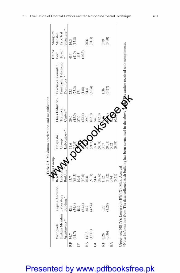
Table7.3
Maxim
um
accelerationandmagnification
Yachiyodal
UnitikaMenshin
Apartments*
KajimaAcoustic
Laboratory
Building*
Okumura
Group
Research
Laboratory
Building*
Obayashi
Group
Laboratory
*
Oires
Industries
Technical
Center*
TakenakaKomuten,
FunabashiTaketomo
Dorm
itory
*
Chiba
Port
Tower
*
Mongumi
Menshin
Typetest
Structure
*
RF
34.7
42.9
45.7
11.6
29.0
23.1
414
16.3
(44.7)
(54.4)
(66.5)
(10.9)
(45.0)
(23.3)
(410)
(15.8)
IF48.9
10.4
26.0
27.0
171
15.5
(63.4)
(10.6)
(43.0)
(22.4)
(148)
(15.3)
BA
131.3
34.7
40.8
20.4
29.0
64.4
20.6
(123.3)
(42.4)
(50.3)
(21.5)
(62.0)
(86.4)
(31.3)
GI
54.6
39.0
54.0
(82.6)
(43.8)
(72.0)
RF
0.26
1.23
1.12
0.57
1.0
1.36
0.79
(0.36)
(1.28)
(1.32)
(0.51)
(0.73)
(0.27)
(0.50)
BA
0.74
0.52
0.54
(0.61)
(0.49)
(0.86)
Upper
rowNS(Y
);Lower
rowEW
(X),Max.Acc:gal
*Note:Inform
ationfrom
Thedata
collectedeach
buildinghasbeennorm
alisedin
theaboveTable.Theauthorreceived
withcompliments.
7.3 Evaluation of Control Devices and the Response-Control Technique 463
www.pdfbo
oksfr
ee.pk
Presented by www.pdfbooksfree.pk
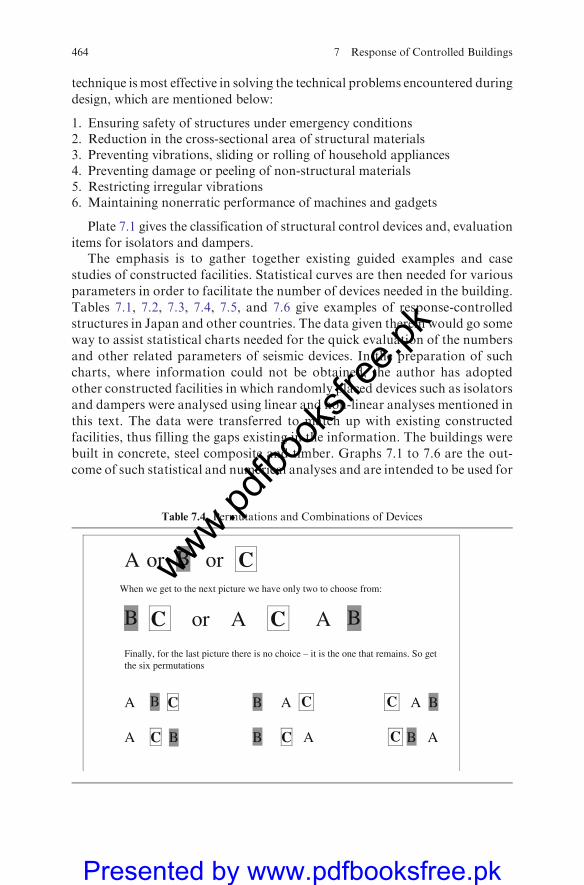
technique is most effective in solving the technical problems encountered during
design, which are mentioned below:
1. Ensuring safety of structures under emergency conditions2. Reduction in the cross-sectional area of structural materials3. Preventing vibrations, sliding or rolling of household appliances4. Preventing damage or peeling of non-structural materials5. Restricting irregular vibrations6. Maintaining nonerratic performance of machines and gadgets
Plate 7.1 gives the classification of structural control devices and, evaluation
items for isolators and dampers.The emphasis is to gather together existing guided examples and case
studies of constructed facilities. Statistical curves are then needed for various
parameters in order to facilitate the number of devices needed in the building.
Tables 7.1, 7.2, 7.3, 7.4, 7.5, and 7.6 give examples of response-controlled
structures in Japan and other countries. The data given therein would go some
way to assist statistical charts needed for the quick evaluation of the numbers
and other related parameters of seismic devices. In the preparation of such
charts, where information could not be obtained, the author has adopted
other constructed facilities in which randomly placed devices such as isolators
and dampers were analysed using linear and non-linear analyses mentioned in
this text. The data were transferred to match up with existing constructed
facilities, thus filling the gaps existing in the information. The buildings were
built in concrete, steel composite and timber. Graphs 7.1 to 7.6 are the out-
come of such statistical and numerical analyses and are intended to be used for
Table 7.4 Permutations and Combinations of Devices
A or B or CWhen we get to the next picture we have only two to choose from:
B C or A C A B
Finally, for the last picture there is no choice – it is the one that remains. So get the six permutations
A B C B A C C A B
A C B B C A C B A
464 7 Response of Controlled Buildings
www.pdfbo
oksfr
ee.pk
Presented by www.pdfbooksfree.pk
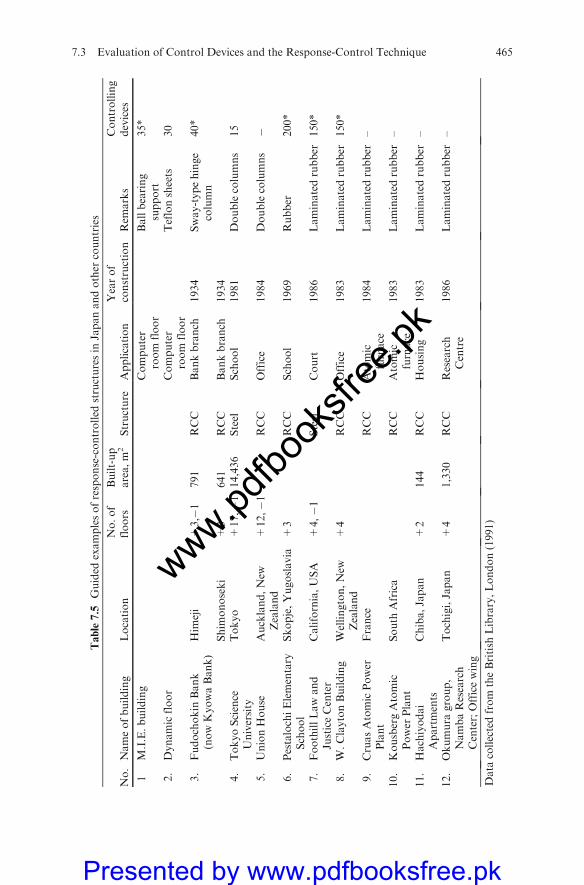
Table7.5
Guided
examplesofresponse-controlled
structuresin
Japanandother
countries
No.Nameofbuilding
Location
No.of
floors
Built-up
area,m
2Structure
Application
Yearof
construction
Rem
arks
Controlling
devices
1M.I.E.building
Computer
room
floor
Ballbearing
support
35*
2.
Dynamicfloor
Computer
room
floor
Teflonsheets
30
3.
Fudochokin
Bank
(nowKyowaBank)
Him
eji
+3,�
1791
RCC
Bankbranch
1934
Sway-typehinge
column
40*
Shim
onoseki
+3
641
RCC
Bankbranch
1934
4.
TokyoScience
University
Tokyo
+17,�1
14,436
Steel
School
1981
Doublecolumns
15
5.
UnionHouse
Auckland,New
Zealand
+12,�1
RCC
Office
1984
Doublecolumns�
6.
PestalochiElementary
School
Skopje,Yugoslavia
+3
RCC
School
1969
Rubber
200*
7.
FoothillLawand
JusticeCenter
California,USA
+4,�1
Steel
Court
1986
Laminatedrubber
150*
8.
W.ClaytonBuilding
Wellington,New
Zealand
+4
RCC
Office
1983
Laminatedrubber
150*
9.
CruasAtomicPower
Plant
France
RCC
Atomic
furnace
1984
Laminatedrubber
–
10.
KousbergAtomic
Power
Plant
South
Africa
RCC
Atomic
furnace
1983
Laminatedrubber
–
11.
Hachiyodai
Apartments
Chiba,Japan
+2
144
RCC
Housing
1983
Laminatedrubber
–
12.
Okumura
group,
NambaResearch
Center;Officewing
Tochigi,Japan
+4
1,330
RCC
Research
Centre
1986
Laminatedrubber
–
Data
collectedfrom
theBritish
Library,London(1991)
7.3 Evaluation of Control Devices and the Response-Control Technique 465
www.pdfbo
oksfr
ee.pk
Presented by www.pdfbooksfree.pk
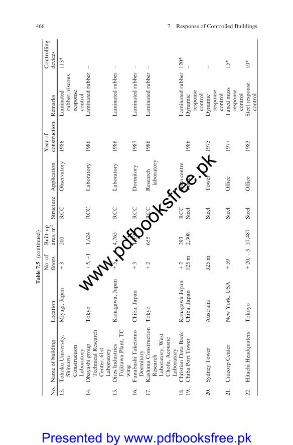
Table7.5
(continued)
No.Nameofbuilding
Location
No.of
floors
Built-up
area,m
2Structure
Application
Yearof
construction
Rem
arks
Controlling
devices
13.
TohokuUniversity,
Shim
azu
Construction
Laboratory
Miyagi,Japan
+3
200
RCC
Observatory
1986
Laminated
rubber,viscous
response
control
113*
14.
Obayashigroup
TechnicalResearch
Center,61st
Laboratory
Tokyo
+5,–1
1,624
RCC
Laboratory
1986
Laminatedrubber
–
15.
Oires
Industries
FujizawaPlant,TC
wing
Kanagawa,Japan
+5
4,765
RCC
Laboratory
1986
Laminatedrubber
–
16.
FunabashiTaketomo
Dorm
itory
Chiba,Japan
+3
1,530
RCC
Dorm
itory
1987
Laminatedrubber
–
17.
Kashim
aConstruction
Research
Laboratory,West
Chofu,Acoustic
Laboratory
Tokyo
+2
655
RCC
Research
laboratory
1986
Laminatedrubber
–
18.
ChristianData
Bank
KanagawaJapan
+2
293
RCC
Data
centre
Laminatedrubber
120*
19.
ChibaPortTower
Chiba,Japan
125m
2,308
Steel
Tower
1986
Dynamic
response
control
–
20.
Sydney
Tower
Australia
325m
Steel
Tower
1975
Dynamic
response
control
–
21.
Citicorp
Center
New
York,USA
+59
Steel
Office
1977
Tuned
mass
response
control
15*
22.
HitachiHeadquaters
Tokoyo
+20,�3
57,487
Steel
Office
1983
Steelresponse
control
10*
466 7 Response of Controlled Buildings
www.pdfbo
oksfr
ee.pk
Presented by www.pdfbooksfree.pk

Table7.5
(continued)
23.
WorldTradeCenter
New
York,USA
+110
Steel
Office
1976
VEM
damper
(viscouselastic
mass)
35*
24.
Columbia
Center
Seattle,USA
+76
Steel
Office
1985
VEM
damper
(viscouselastic
mass)
25.
RadarConstruction
Chiba,Japan
Steel
Instrument
platform
1980
Roller
bearing
35
26.
Christchurchchim
ney
Christchurch,New
Zealand
35m
RCC
Chim
ney
Steelresponse
control
60*
27.
Commerce,Cultural
Saitama,Japan
+30
Steel
Office
1987
Frictionresponse
control
38
28.
Fujita
Industries
TechnicalResearch
Laboratory
(6th)
Kanagawa,Japan
+3
3,952
RCC
Research
center
Laminatedrubber
80*
29.
ShibuyaShim
izuNo.1
Building
Tokoyo
+5,�1
3,385
RCC
Office
Laminatedrubber
80*
30.
FukumiyaApartments
Tokoyo
+4
682
RCC
Cooperative
housing
Laminatedrubber
–
31.
LambesoC.E.S
France
+3
4,590
RC prefab
School
1978
Laminatedrubber
–
Note:+
Indicatesfloors
abovegroundand–indicatesfloors
belowground.
*Comparedandtested
onthebasisofdynamicnon-linearthree-dim
ensionalfiniteelem
entAnalysis.
Note:Data
collectedfrom
sources
Note:Data
collectedfrom
cases1to
12from
locationsgiven
intheTable
andplace
them
ingiven
order.Withcompliments
from
organisations
mentioned
initem
sNo.1to
31.Theauthoracknowledges
thedata
withthanks.
7.3 Evaluation of Control Devices and the Response-Control Technique 467
www.pdfbo
oksfr
ee.pk
Presented by www.pdfbooksfree.pk

Table7.6
Case
studiesofearthquakeconstructed
facilities
Item
Hachiyaapartmentsz
Christiandata
centerØz
Okumura
groupØ
Ø
Designed
by
TokyoBuildingResearchCenter
TokyoBuildingResearchCenter,
Unitika
TokyoBuildingResearchCenter,
Okumura
group
Yearofapproval;No.455
2Novem
ber
1982;Kana61
19Novem
ber
1985;Tochi37
24Decem
ber
1985;
No.offloors
+2
+2,�1
+4
Built-uparea,m
260.18
226.21
348.18
Application
Housing(residential)
Data
house
Researchcentre
Structure
RCCframe(shearwall)
RCCframe(shearwall)
RCCframe
Foundation
Raftfoundationwithcastin
situ
piles
Deepfoundation
RCCcastin
situ
raft
Isolator:Dim
ensions,mm
82�
300dia
Rubber
5thick�
300dia
(12layers)
Rubber
7thickthick�
500dia
(14layers)
Numbers
(6)(computed7)
(32)(28)
(25)(21)
Supportingforce
s=45kg/cm
2,0.5
t/cm
(32t)
s=60kg/cm
2,0.5
t/cm
(42.5
t)s=
60kg/cm
2,0.86t/cm
(120t)
Response-controldevice
FrictionforcebetweenPCplates
Usesplasticdefomationofsteelbars
bentto
makealoop(8
nos)
Usesplasticdeform
ationofsteelb
arsbent
tomakealoop(12nos)
Shearforcecoefficient
usedin
design
0.2
0.15
0.15
Fundament
Small
period
deform
ation
1.83cm
1.4
cm1.4
cm
Large
deform
ation
1.9
cm2.1
cmIncidentseismicwave
El-Centro1940(N
S)
El-Centro1940(N
S)
El-Centro1940(N
S)
Hachinohe1968(N
S)
Hachinohe1968(N
S)
Taft1952(EW)
Hachinohe1986(EW)
Taft1952(EW)
Hachinohe1968(N
S)
Taft1952(EW)
Inputlevel
300gal
300gal,450gal
300gal,450gal
Note:(*)computedandtested
onthebasisofdynamicnon-linearthree-dim
ensionalanalysisusingfiniteelem
ent.
(Ø)Actuallyprovided.
Note:Data
collectedfrom
thearchives
British
Library
forHuchiyaapartments
(z),
christiandata
center[Øz]
andokumura
group[Ø
Ø],with
compliments.
468 7 Response of Controlled Buildings
www.pdfbo
oksfr
ee.pk
Presented by www.pdfbooksfree.pk
evaluating the initial number of devices, displacements, velocities and accel-
erations for various heights and floor areas of the buildings. This procedure
has cut down the time and effort of making decisions regarding devices and
building final displacement, velocity and acceleration. The exact analysis for a
particular building will be carried out both with and without such devices. The
extent of control within specified limitations will be known. The limitations on
the following will be adhered to:
(a) Response acceleration(b) Response relative displacement (using linear, non-linear and damage
analyses)(c) Response material stress(d) Physical positioning of devices in a specific layout in three dimensions
The variables concerning (d) shall require the knowledge of total building
floor area, standard area per floor, floor height and final building height. Once
the total number of devices ‘‘S’’ is known from the graph, the next step is to
initially spread these devices across the building structure when the above
requirements are met. Various methods are available and their boundary con-
ditions must be such that the requisite number must easily be accommodated
after the analytical decisions are made. In this text the selected method is based
on permutation and/or combination. The permutation is for single-type device
and combination is for two or more types of devices placed in sequence or in
others to reduce drift, acceleration and velocity commensurate with the codified
methods and clauses noted in design practices. This method cuts down the time
and cost involved in arriving at the optimum choice finally placed before a
specific computer program to assess andmeet the targets given by designers and
clients. It is therefore necessary to remind the reader about the method.
7.3.2 Permutations and Combinations
7.3.2.1 Permutations
A permutation for the devices of identical shape, make and performance shall be
the ‘‘rearrangement number’’ or ‘‘order’’ in specific area of a floor from an ordered
list ‘‘S’’ required for a building within specific seismic zone. The rearrangement of
devices in permutationwill finally determine the optimumpositions, whenput to a
specific analysis-cum-computer program, such that the targets are met.For example, the number of permutations for devices {1, 2}, namely {1, 2}
and {2,1}, shall be 2! = 2 � 1 =2 two places two permutations in two
positions; 3! = 3 � 2 � 1=6 three places and six permutations in three
positions for the devices to be placed at the floor level. In order to further
explain, the 3! would be in the following six set-up and in six orders as
7.3 Evaluation of Control Devices and the Response-Control Technique 469
www.pdfbo
oksfr
ee.pk
Presented by www.pdfbooksfree.pk
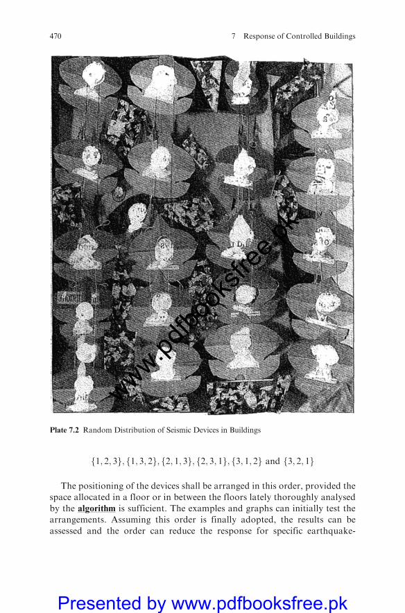
1; 2; 3f g; 1; 3; 2f g; 2; 1; 3f g; 2; 3; 1f g; 3; 1; 2f g and 3; 2; 1f g
The positioning of the devices shall be arranged in this order, provided the
space allocated in a floor or in between the floors lately thoroughly analysed
by the algorithm is sufficient. The examples and graphs can initially test the
arrangements. Assuming this order is finally adopted, the results can be
assessed and the order can reduce the response for specific earthquake-
Plate 7.2 Random Distribution of Seismic Devices in Buildings
470 7 Response of Controlled Buildings
www.pdfbo
oksfr
ee.pk
Presented by www.pdfbooksfree.pk
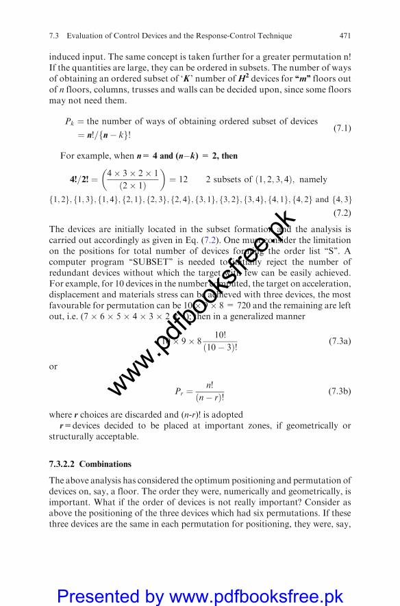
induced input. The same concept is taken further for a greater permutation n!If the quantities are large, they can be ordered in subsets. The number of waysof obtaining an ordered subset of ‘K ’ number ofH2 devices for ‘‘m’’ floors outof n floors, columns, trusses and walls can be decided upon, since some floorsmay not need them.
Pk ¼ the number of ways of obtaining ordered subset of devices
¼ n!=fn� kg!(7:1)
For example, when n= 4 and (n�k) = 2, then
4!=2! ¼ 4� 3� 2� 1
ð2� 1Þ
�¼ 12 2 subsets of 1; 2; 3; 4ð Þ; namely
�
1; 2gf ; 1; 3f g; 1; 4f g; 2; 1f g; 2; 3f g; 2; 4f g; 3; 1f g; 3; 2f g; 3; 4f g; 4; 1f g; 4; 2f g and 4; 3f g(7:2)
The devices are initially located in the subset formation and the analysis iscarried out accordingly as given in Eq. (7.2). One must consider the limitationon the positions for total number of devices forming the order list ‘‘S’’. Acomputer program ‘‘SUBSET’’ is needed to initially reject the number ofredundant devices without which the target with few can be easily achieved.For example, for 10 devices in the number computed, the target on acceleration,displacement and materials stress can be achieved with three devices, the mostfavourable for permutation can be 10� 9� 8 = 720 and the remaining are leftout, i.e. (7 � 6 � 5 � 4 � 3 � 2 � 1); then in a generalized manner
10� 9� 810!
10� 3ð Þ! (7:3a)
or
Pr ¼n!
n� rð Þ! (7:3b)
where r choices are discarded and (n-r)! is adoptedr=devices decided to be placed at important zones, if geometrically or
structurally acceptable.
7.3.2.2 Combinations
The above analysis has considered the optimum positioning and permutation ofdevices on, say, a floor. The order they were, numerically and geometrically, isimportant. What if the order of devices is not really important? Consider asabove the positioning of the three devices which had six permutations. If thesethree devices are the same in each permutation for positioning, they were, say,
7.3 Evaluation of Control Devices and the Response-Control Technique 471
www.pdfbo
oksfr
ee.pk
Presented by www.pdfbooksfree.pk

all A, B and C, however they are positioned. ‘‘They were only one combination’’.Hence for 3!, i.e. six permutations, they have one combination. Three deviceswill be ‘‘one set’’. The same will be true for ‘‘each group’’ of three devices as aboveas choosing 720 permutations when choosing 3 devices from ‘‘10’’. So the
number 3! of sets of 3 from 10 can be arranged in combinations as 7203!¼ 120.
In general, it can be further written in shorthand as
number of combinations ¼ total number of permutations for positioning devices
number of permutations of each set of devices
(7:4)
In the same way that permutations have shorthand, combinations havesimilar shorthand. All one has to do is to divide the total number of permuta-tions by the number of permutations in each set. So, the right-hand side of thefollowing equation is the same as the equation for the number of permutationsexcept for an additional r! term in the divisor which corrects the number ofpermutations of each set of devices for true positioning.
C ¼ n!
r! n� rð Þ!(7:5)
7.4 Permutations and Combinations of Devices
When one talks of permutations and combinations one often uses the two termsinterchangeably (Suggestion: ‘‘When talking of permutations and combina-tions, these terms are oftentimes used interchangeably.’’) In mathematics, how-ever, the two each have very specific meanings, and this distinction often causesproblems. (Suggestion: In mathematics, however, each of these terms carries adistinctive meaning, which can cause confusion.’’)
In brief, the permutation of a number of devices is the number of differentways they can be placed, i.e. which is first, second, third, etc. If one wishes tochoose some device from a larger number of devices, the way one positions thechosen device is also important. With combinations, on the other hand, onedoes not consider the order in which devices were chosen or placed, just whichdevices were chosen. They could be devices chosen from Plate 7.1.
One can summarise them asPermutations – position important (although choice may also be important)Combinations – chosen devices important, which may help one to remember
which is which and the difference between them for thepurpose of recognition in devices
As mentioned above, there is an important difference between permutationsand combinations. In this case, for permutations the order of events is
472 7 Response of Controlled Buildings
www.pdfbo
oksfr
ee.pk
Presented by www.pdfbooksfree.pk
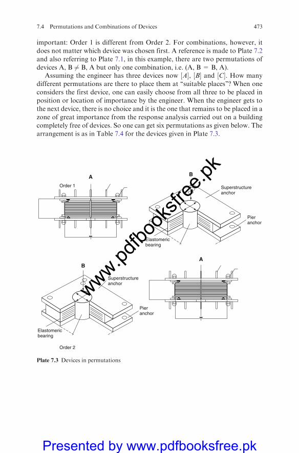
important: Order 1 is different from Order 2. For combinations, however, it
does not matter which device was chosen first. A reference is made to Plate 7.2
and also referring to Plate 7.1, in this example, there are two permutations of
devices A, B 6¼ B, A but only one combination, i.e. (A, B = B, A).Assuming the engineer has three devices now A½ �, B½ � and C½ �. How many
different permutations are there to place them at ‘‘suitable places’’? When one
considers the first device, one can easily choose from all three to be placed in
position or location of importance by the engineer. When the engineer gets to
the next device, there is no choice and it is the one that remains to be placed in a
zone of great importance from the response analysis carried out on a building
completely free of devices. So one can get six permutations as given below. The
arrangement is as in Table 7.4 for the devices given in Plate 7.3.
Superstructureanchor
Pieranchor
Elastomericbearing
Order 1
A
A
B
B
Superstructureanchor
Pieranchor
Order 2
Elastomericbearing
Plate 7.3 Devices in permutations
7.4 Permutations and Combinations of Devices 473
www.pdfbo
oksfr
ee.pk
Presented by www.pdfbooksfree.pk
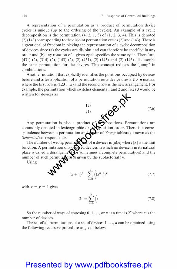
A representation of a permutation as a product of permutation device
cycles is unique (up to the ordering of the cycles). An example of a cyclic
decomposition is the permutation (4, 2, 1, 3) of (1, 2, 3, 4). This is denoted
(2) (143) corresponding to the disjoint permutation cycles (2) and (143). There is
a great deal of freedom in picking the representation of a cyclic decomposition
of devices since (a) the cycles are disjoint and can therefore be specified in any
order and (b) any rotation of a given cycle specifies the same cycle. Therefore,
(431) (2), (314) (2), (143) (2), (2) (431), (2) (143) and (2) (143) all describe
the same permutation for the devices. This concept reduces the ‘‘jump’’ in
combinations.Another notation that explicitly identifies the positions occupied by devices
before and after application of a permutation on n device uses a 2 � n matrix,
where the first row is (123 . . .n) and the second row is the new arrangement. For
example, the permutation which switches elements 1 and 2 and fixes 3 would be
written for devices as
123
213(7:6)
Any permutation is also a product of transpositions. Permutations are
commonly denoted in lexicographic or transposition order. There is a corre-
spondence between a permutation and a pair of Young tableaux known as the
Schensted correspondence.The number of wrong permutations of n devices is [n!/e] where [x] is the nint
function. A permutation of n ordered devices in which no device is in its natural
place is called a derangement (or sometimes a complete permutation) and the
number of such permutations is given by the subfactorial !n.Using
xþ yð Þn¼Xxr¼0ðÞn
rxn�ryr (7:7)
with x = y = 1 gives
2x ¼Xxr¼0ðÞn
r(7:8)
So the number of ways of choosing 0, 1,. . ., or n at a time is 2n where n is the
number of devices.The set of all permutations of a set of devices 1, . . ., n can be obtained using
the following recursive procedure as given below:
474 7 Response of Controlled Buildings
www.pdfbo
oksfr
ee.pk
Presented by www.pdfbooksfree.pk
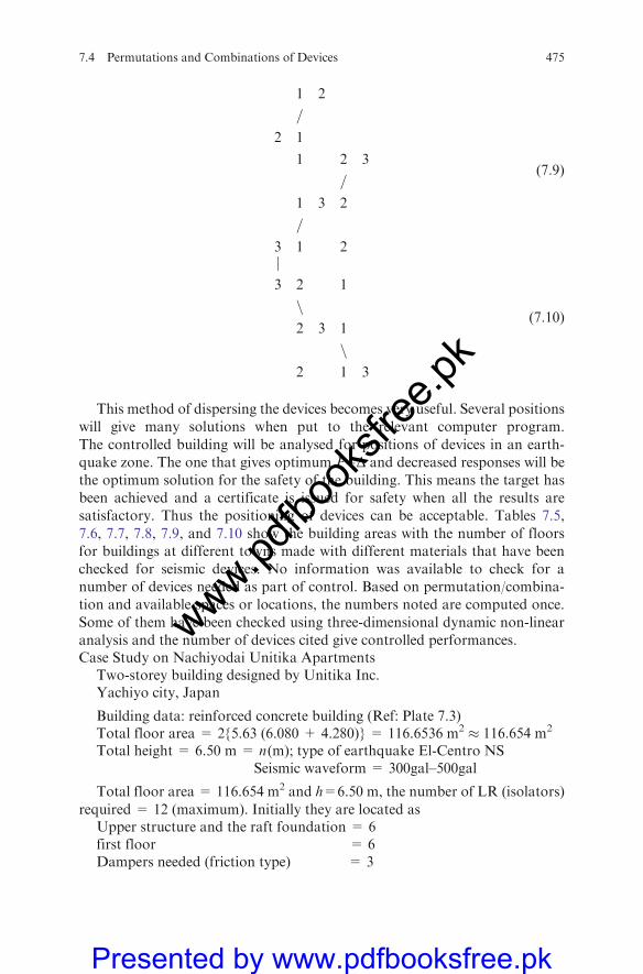
1 2
=
2 1
1 2 3
=
1 3 2
=
3 1 2
(7:9)
j3 2 1
n2 3 1
n2 1 3
(7:10)
This method of dispersing the devices becomes very useful. Several positionswill give many solutions when put to the relevant computer program.
The controlled building will be analysed for positions of devices in an earth-quake zone. The one that gives optimum P�D and decreased responses will bethe optimum solution for the safety of the building. This means the target hasbeen achieved and a certificate is issued for safety when all the results aresatisfactory. Thus the positioning of devices can be acceptable. Tables 7.5,
7.6, 7.7, 7.8, 7.9, and 7.10 show the building areas with the number of floorsfor buildings at different towns made with different materials that have beenchecked for seismic devices. No information was available to check for anumber of devices needed as part of control. Based on permutation/combina-tion and available spaces or locations, the numbers noted are computed once.
Some of them have been checked using three-dimensional dynamic non-linearanalysis and the number of devices cited give controlled performances.Case Study on Nachiyodai Unitika Apartments
Two-storey building designed by Unitika Inc.Yachiyo city, Japan
Building data: reinforced concrete building (Ref: Plate 7.3)Total floor area = 2{5.63 (6.080 + 4.280)} = 116.6536 m2 � 116.654 m2
Total height = 6.50 m = n(m); type of earthquake El-Centro NSSeismic waveform = 300gal–500gal
Total floor area = 116.654 m2 and h=6.50 m, the number of LR (isolators)
required = 12 (maximum). Initially they are located asUpper structure and the raft foundation = 6first floor = 6Dampers needed (friction type) = 3
7.4 Permutations and Combinations of Devices 475
www.pdfbo
oksfr
ee.pk
Presented by www.pdfbooksfree.pk
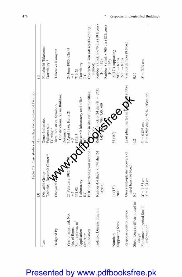
Table7.7
Case
studiesofearthquakeconstructed
facilities
(3)
(4)
(5)
Item
ObayashiGroup
DieresIndustries
FunabashiTaketomo
TechnicalResearchCenter*
Fujizawasite
Dorm
itory
*TCwing*
Designed
by
ObayashiGroup
Oires
Industries,Symiono
Constructions,YasuiBuilding
TakenakaKomyten
Designers
Yearofapproval;No.
27February
1986;Tok.30
7April1986;Kana21
24June1986;Chi43
No.offloors
+5
+5
+3
Built-uparea,m
2351.92
1136.5
719.28
Application
Laboratory
Researchlaboratory
andoffice
Dorm
itory
Structure
RC
RC
RC
Foundation
PHCtie(cem
entgroutmethod)
Concretein
situ
raft(earth-drilling
method)
Concretein
situ
raft(earth-drilling
method)
Isolator:Dim
ensions,mm
Rubber
4.4
thick�
740dia
(61
layers)
Rubber
10thick�
24dia
(H=
363),
OD
=650,700,750,800
Rubber
7thick�
670dia
(19layers)
(H=
187)
Rubber
8thickx700dia
(18layers)
(H=
195)
Numbers
14(15*)
35(38*)
14(17*)supporting
Supportingforce
200t
200t!
6nos
150t!
8nos
Response-controldevice
Useselasto-plasticrecoveryof
steelbars
(96Nos.)
Leadpluginserted
inlaminatedrubber
Viscousdamper
(8Nos.)
Shearforcecoefficientusedin
design
0.5
0.2
0.15
FundamentalperiodSmall
deform
ation
X=
1.33cm
Y=
1.24cm
X=
0.895cm
Y=
0.908cm
(at50%
deflection)
X=
2.09cm
476 7 Response of Controlled Buildings
www.pdfbo
oksfr
ee.pk
Presented by www.pdfbooksfree.pk

Table7.7
(continued)
Largedeform
ation
X=
3.12cm
X=
2.143cm
Y=
2.10cm
Y=
3.08cm
Y=
2.148cm
(at100%
deflection)
Incidentseismicwave
El-Centro1940(N
S)
El-Centro1940(N
S)
El-Centro1940(N
S)
Hachinohe1968(N
S)
Hachinohe1968(N
S)
Taft1952(EW)
Hachinohe1968(EW)
Hachinohe1968(EW)
Tokyo1o11956(N
S)
Taft1952(EW)
Taft1952(EW)
Hachinohe1968(N
S)
Man-m
adeearthquake
KT0081980(N
S)
Man-m
adeearthquake
2waves
Man-m
adeearthquake
4waves
2waves
Inputlevel
25cm
/sec,50cm
/s25cm
/sec,50cm
/s25cm
/sec,50cm
/s
Note:(*)computedandtested
onthebasisofdynamicnon-linearthree-dim
ensionalanalysisusingfiniteelem
ent.
*Note:Data
collectedwiththecomplimentsofrespectivecompanies.
7.4 Permutations and Combinations of Devices 477
www.pdfbo
oksfr
ee.pk
Presented by www.pdfbooksfree.pk

Table7.8
Case
studiesofearthquakeconstructed
facilities
Item
Kashim
aConstructionsResearch
Center(reapplied)*
ChristianData
Apartments*
Fukumiya*
Center,NishiChofu
Acciystus
Designed
by
Kashim
aConstructions
TokyoBuildingResearchCenter
Okumura
Group
Designrequirem
ents
Reduce
seismicinputandinsulate
(isolate)from
Earth’svibrations
Antiseismic.Preventanydamageto
storedgoods
Safety
ofbuilding.Added
valuein
business
Yearofapproval;No.
Tok473
5Decem
ber
1986;
3March1987;Tok44
No.offloors
+2
+2
+4
Built-uparea,m
2379.10
149.43
225.40
Application
Researchlaboratory
Data
house
Cooperativehousing
Structure
RC
RC
RC
Foundation
Concretein
situ
raft(deepfoundation)
Deepfoundation
Concretein
situ
raft
(miniature
earth-drilling
method)
Isolator:Dim
ensions,mm
320�
1340(48thick�
5dial);308�
1080(38thick�
6dia)(25layers)
4thick�
435dia
Dnamic
Numbers
18
12
Non-linear
Supporting
165t:1340dia
s=60kg/cm
2;0.55
F.E.Analysis
force
100t:1080dia
t/cm
(90t)
Respones-
controldevice
Elasto-plasticdamper
usingmildsteel
14T15
Usesplasticdeform
ationofsteel
bars
bentto
makealoop6T8
Usesplasticdeform
ationof
steelbars
bentto
makea
loop7T10
f
478 7 Response of Controlled Buildings
www.pdfbo
oksfr
ee.pk
Presented by www.pdfbooksfree.pk

Table7.8
(continued)
Shearforcecoefficient
usedin
design
0.2
0.15
0.2
Primary
Small
perioddeform
ation
X=
0.828cm
Y=
0.809cm
1.3
cm1.4
cm
Largedeform
ation
1.80cm
1.9
cm2.2
cmIncidentseismicwave
EICentro1940(N
S)
EICentro1940(N
S)
EICentro1940(N
S)
Taft1952(EW)
Taft1952(EW)
Taft1952(EW)
Tokyo1011956(N
S)
Hachinohe1968(N
S)
Tokyo1011956(N
S)
Sendai
Hachinohe1968(N
S)
THO38-1
1978(EW)
Inputlevel
25cm
/s,50cm
/s300gal,450gal
25cm
/s,50cm
/s
NOTE:(*)computedandtested
onthebasisofdynamicnon-linearthree-dim
ensionalanalysisusingfiniteelem
ent.
()Actuallyprovided.
*Data
collectedfrom
thesecompaniesandpresentedin
thegiven
form
at.Withcomplimentsfrom
theseconstructors
inJapan.
7.4 Permutations and Combinations of Devices 479
www.pdfbo
oksfr
ee.pk
Presented by www.pdfbooksfree.pk
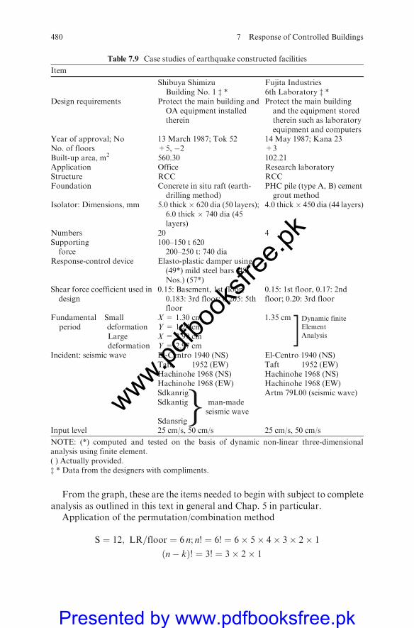
From the graph, these are the items needed to begin with subject to complete
analysis as outlined in this text in general and Chap. 5 in particular.Application of the permutation/combination method
S ¼ 12; LR=floor ¼ 6 n; n! ¼ 6! ¼ 6� 5� 4� 3� 2� 1
n� kð Þ! ¼ 3! ¼ 3� 2� 1
Table 7.9 Case studies of earthquake constructed facilities
Item
Shibuya Shimizu Fujita IndustriesBuilding No. 1 z * 6th Laboratory z *
Design requirements Protect the main building andOA equipment installedtherein
Protect the main buildingand the equipment storedtherein such as laboratoryequipment and computers
Year of approval; No 13 March 1987; Tok 52 14 May 1987; Kana 23No. of floors +5, �2 +3Built-up area, m2 560.30 102.21Application Office Research laboratoryStructure RCC RCCFoundation Concrete in situ raft (earth-
drilling method)PHC pile (type A, B) cementgrout method
Isolator: Dimensions, mm 5.0 thick� 620 dia (50 layers);6.0 thick � 740 dia (45layers)
4.0 thick� 450 dia (44 layers)
Numbers 20 4Supporting 100–150 t 620force 200–250 t: 740 dia
Response-control device Elasto-plastic damper using(49*) mild steel bars (48Nos.) (57*)
Shear force coefficient used indesign
0.15: Basement, 1st floor;0.183: 3rd floor; 0.205: 5thfloor
0.15: 1st floor, 0.17: 2ndfloor; 0.20: 3rd floor
Fundamental Smallperiod deformation
X = 1.30 cmY = 1.24 cm
1.35 cm
Largedeformation
X = 2.99 cmY = 2.97 cm
Incident: seismic wave El-Centro 1940 (NS) El-Centro 1940 (NS)Taft 1952 (EW) Taft 1952 (EW)Hachinohe 1968 (NS) Hachinohe 1968 (NS)Hachinohe 1968 (EW) Hachinohe 1968 (EW)Sdkanrig Artm 79L00 (seismic wave)Sdkantig man-made
seismic waveSdansrig
Input level 25 cm/s, 50 cm/s 25 cm/s, 50 cm/s
NOTE: (*) computed and tested on the basis of dynamic non-linear three-dimensionalanalysis using finite element.( ) Actually provided.z * Data from the designers with compliments.
g
�Dynamic finiteElementAnalysis
480 7 Response of Controlled Buildings
www.pdfbo
oksfr
ee.pk
Presented by www.pdfbooksfree.pk

Pk ¼ n!n�kð Þ!
¼ 120
Cnr ¼
120
3� 2� 1¼ 20 positioning for combination
The requisite floors:
SþDampers ¼ 12þ 7 ¼ 19 � 20"
Two floors are okay adopted computed
Table 7.10 Case studies of earthquake constructed facilities
Item (11) (12)
Inorganic Materials ResearchCenter, Vibration-free Wing
Shimizu Constructions,Chuchiura Branch, newbuilding
1 2 3Designed by Secretariat of the Ministry of
Construction, PlanningBureau
Shimizu Constructions
Design requirements Protect the main building andresearch equipment storedtherein
Year of approval June 1987 June 1987No. of floors +1 +4Built-up area, m2 8,341 (old – 7,725; new – 616) 170.366Application Research centre Office, company housingStructure RCC RCCFoundation PHC raft (type A) blast method PHC raft (type B, C) method
using earth augerIsolator: Dimensions, mm 3.2 thick � 420 dia (62 layers) 6.0 thick � 450 dia; 6.0 � 500;
6.0 � 550 (31 layers)Number 32 14Supporting force 65 t (max 80 t) 51–165 tResponse-control device Elasto-plastic damper using
mild steel bars (108 nos.)(112*)
Lead plug inserted inlaminated rubber (112*)
Shear force coefficient used indesign
0.15 All floors 0.15
Fundamental Small X = 1.17 cm X = 0.77 cmperiod deformation Y = 1.17 cm Y = 0.77 cm
Large X = 2.26 cm X = 2.33 cmdeformation Y = 2.26 cm Y = 2.33 cm
Incident seismic wave El-Centro 1940 (NS) El-Centro 1940 (NS)Taft 1952 (EW) Taft 1952 (EW)Hachinohe 1968 (NS) Hachinohe 1968 (NS)Hachinohe 1968 (EW) Ibaragi 606 1964 (NS)Tsukuba 85 NSTsukuba 85 EW ObservedTsukuba 86 NS seismic wavesTsukuba 86 EW
Input level 25 cm/s, 50 cm/s 35 cm/s, 50 cm/s
NOTE:(*) computed and tested on the basis of dynamic non-linear three-dimensional analysis usingfinite element.( ) Actually provided.Data under 1,2,3 are obtained by the author with compliments.
�
g
�Dynamic FiniteElementAnalysis
7.4 Permutations and Combinations of Devices 481
www.pdfbo
oksfr
ee.pk
Presented by www.pdfbooksfree.pk

These are now to be tested for a given layout using the program ISOPAR and
then finally checked against the design given by Unita Inc., Japan.
Data for Raft foundation For soil–structure interactionGround propertyFoundation depth Raft foundation. Formation GL-1.15 mSoil property and N value
GL-m 0–2.8 2.8–3.9 3.9–10.8 10.8–12.7 12.7
Soil Red loam Red aboveloam
finesand
very finesand
Fine sand loambelow
N value <4 1.4 4–17 25–27 >50
Permissible pile resistance 6.0 t/m2 = 60 KN/m2
Outline of the structure
Foundation
Ground type: Raft foundation, supported directly on loam-type soil.Formation depth:
Foundationstructure:
GL-1.15 m
Maximum contact: Long term: 4.81 t/m2 = 48.1 KN/m2
Pressure: Short term: –
Case Study 7.1 A Two-Storey Building
Description of the structureA reference is made to Plate 7.4. It is an RCC framed structure with the
following details of the elements:
482 7 Response of Controlled Buildings
www.pdfbo
oksfr
ee.pk
Presented by www.pdfbooksfree.pk
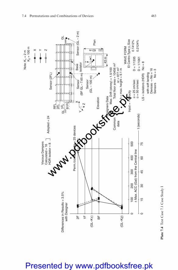
Sen
sor
(BF
GL
–7.
65 m
)
Sen
sor
(2F
L)R
FL
2FL
1FL
B1F
L
GL
Not
e: K
1 =
2 m
K2
= 1
00 m
Sen
sor
(GL
– 10
0 m
)
Ele
vatio
n
Des
igne
rs D
ata
Com
mon
data
Inpu
t = –
Vel
ocity
u =
25
cm/s
ec
WA
VE
FO
RM
El C
entr
o Ty
pe c
i Siz
e0.
1412
%
0.21
24%
u =
50
cm/s
ec
LS =
isol
ator
s (H
DR
) N
o =
8D
= 1
/106
1
D =
1/1
335
with
sof
t lan
ding
Dev
ices
→ N
o =
16
Sen
sors
No
= 3
Max
. Drif
t (st
orey
) =
1.5
/100
Tota
l flo
or a
rea
= 1
0456
m2
or =
977
m2
h =
max
. hei
ght =
9.1
m
Pla
n
43 m
63 m
Bas
eis
olat
orS
enso
r (G
L –
2 m
)
0
(GL–
K2)BF
(GL–
K1)1F
Diff
eren
ces
in R
esul
ts =
3.5
%w
ith D
esig
ner
2F
015
30
± M
ax. A
CC
(G
al)
from
the
Cen
tral
line
4560
75t (
seco
nds)
100
200
300
400
500
X Y Z
Y
x
YZ
XP
erm
./com
b. r
esul
ts =
25
devi
ces
Vis
cous
Dam
pers
Cal
cula
ted
= 1
6H
DR
isol
ator
= 8
Ado
pted
= 2
4
GL
• •
{
Plate
7.4
TestCase
7.1
Case
StudyI
7.4 Permutations and Combinations of Devices 483
www.pdfbo
oksfr
ee.pk
Presented by www.pdfbooksfree.pk
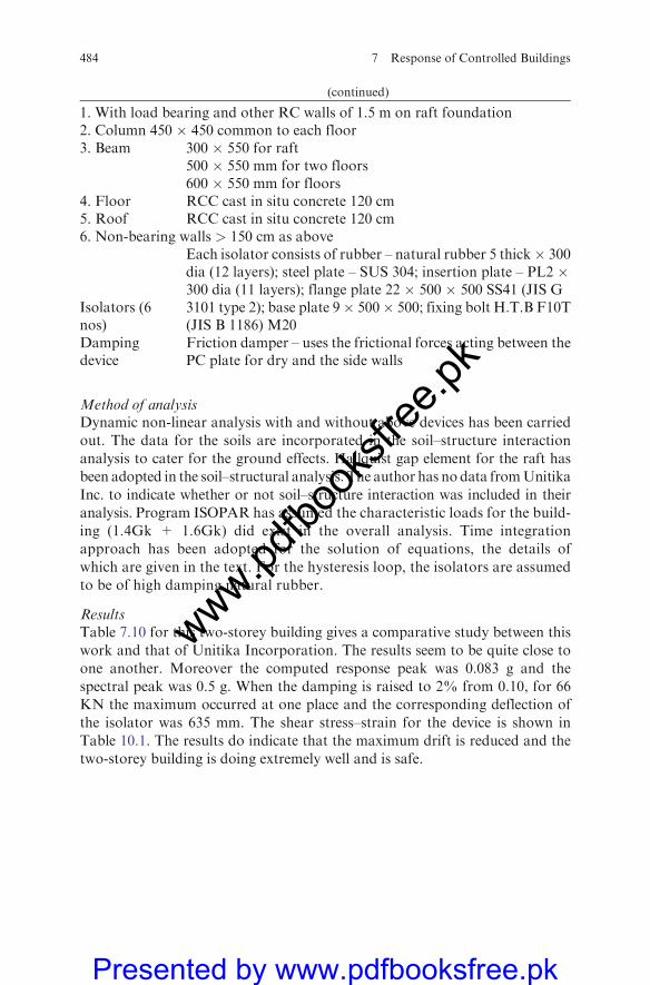
(continued)
1. With load bearing and other RC walls of 1.5 m on raft foundation2. Column 450 � 450 common to each floor3. Beam 300 � 550 for raft
500 � 550 mm for two floors600 � 550 mm for floors
4. Floor RCC cast in situ concrete 120 cm5. Roof RCC cast in situ concrete 120 cm6. Non-bearing walls > 150 cm as above
Isolators (6nos)
Each isolator consists of rubber – natural rubber 5 thick� 300dia (12 layers); steel plate – SUS 304; insertion plate – PL2 �300 dia (11 layers); flange plate 22 � 500 � 500 SS41 (JIS G3101 type 2); base plate 9� 500� 500; fixing bolt H.T.B F10T(JIS B 1186) M20
Dampingdevice
Friction damper – uses the frictional forces acting between thePC plate for dry and the side walls
Method of analysisDynamic non-linear analysis with and without above devices has been carried
out. The data for the soils are incorporated in the soil–structure interaction
analysis to cater for the ground effects. Hallquist gap element for the raft has
been adopted in the soil–structural analysis. The author has no data fromUnitika
Inc. to indicate whether or not soil–structure interaction was included in their
analysis. Program ISOPAR has assumed the characteristic loads for the build-
ing (1.4Gk + 1.6Gk) did exist in the overall analysis. Time integration
approach has been adopted for the solution of equations, the details of
which are given in the text. For the hysteresis loop, the isolators are assumed
to be of high damping natural rubber.
ResultsTable 7.10 for this two-storey building gives a comparative study between this
work and that of Unitika Incorporation. The results seem to be quite close to
one another. Moreover the computed response peak was 0.083 g and the
spectral peak was 0.5 g. When the damping is raised to 2% from 0.10, for 66
KN the maximum occurred at one place and the corresponding deflection of
the isolator was 635 mm. The shear stress–strain for the device is shown in
Table 10.1. The results do indicate that the maximum drift is reduced and the
two-storey building is doing extremely well and is safe.
484 7 Response of Controlled Buildings
www.pdfbo
oksfr
ee.pk
Presented by www.pdfbooksfree.pk
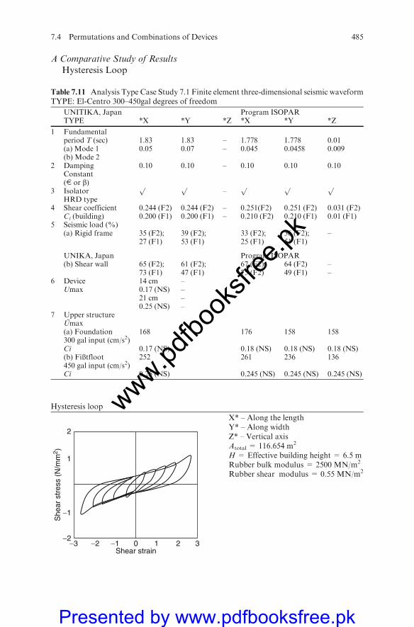
A Comparative Study of ResultsHysteresis Loop
Hysteresis loop
X* – Along the lengthY* – Along widthZ* – Vertical axisAtotal = 116.654 m2
H = Effective building height = 6.5 mRubber bulk modulus = 2500 MN/m2
Rubber shear modulus = 0.55 MN/m2
−1
1
2
−2−3 −2 −1 0
Shear strain
She
ar s
tres
s (N
/mm
2 )
1 2 3
Table 7.11 Analysis Type Case Study 7.1 Finite element three-dimensional seismic waveformTYPE: El-Centro 300–450gal degrees of freedom
UNITIKA, Japan Program ISOPARTYPE *X *Y *Z *X *Y *Z
1 Fundamentalperiod T (sec) 1.83 1.83 – 1.778 1.778 0.01(a) Mode 1 0.05 0.07 – 0.045 0.0458 0.009(b) Mode 2
2 Damping 0.10 0.10 – 0.10 0.10 0.10Constant(E or b)
3 Isolatorp p
–p p p
HRD type4 Shear coefficient 0.244 (F2) 0.244 (F2) – 0.251(F2) 0.251 (F2) 0.031 (F2)
Ci (building) 0.200 (F1) 0.200 (F1) – 0.210 (F2) 0.210 (F1) 0.01 (F1)5 Seismic load (%)
(a) Rigid frame 35 (F2); 39 (F2); 33 (F2); 36 (F2); –27 (F1) 53 (F1) 25 (F1) 51 (F1)
UNIKA, Japan Program ISOPAR(b) Shear wall 65 (F2); 61 (F2); 67 (F2); 64 (F2) –
73 (F1) 47 (F1) 75 (F2) 49 (F1) –6 Device 14 cm –
Umax 0.17 (NS) –21 cm –0.25 (NS) –
7 Upper structureUmax(a) Foundation300 gal input (cm/s2)
168 176 158 158
Ci 0.17 (NS) 0.18 (NS) 0.18 (NS) 0.18 (NS)(b) Fißtfloot450 gal input (cm/s2)
252 261 236 136
Ci 0.25 (NS) 0.245 (NS) 0.245 (NS) 0.245 (NS)
7.4 Permutations and Combinations of Devices 485
www.pdfbo
oksfr
ee.pk
Presented by www.pdfbooksfree.pk

Case Study 7.2Obayashi-Gumi Technical Research Center Laboratory 61 Designed By
Obayashi-Gumi Ltd, Tokyo, Japan
Building Data: Reinforced concrete rigid frame building with RCC seismicwall
Total floor area: 1623.89 m2, total height = 22.80 m = h (m)Area/floor: 328.75m2, Type of earthquake waveform: El-Centro with
acceleration amplitude 300–450 cm/s2
Total floors: above ground = 5Penthouse = 1
Dampers – 24 nos, they are positioned. as a set of 4 Total No = 96.Isolators – 14 no, with ABCD permutation + combination
Total No computed = 98
Soil Property And Foundation DataNote: These data are used for soil–structure interaction analysis
Ground propertyFoundation depthPHC pile
Formation GL-1.775 mPile depth, formationGL-7.0 m
Soil property andN value
GL-m 0–0.7 m 0.7–6.2 m > 6.2 m
Soil type Red loam Loam Gravel
N value – 2.3 >50
Permissible pile resistance PHC pile (Type A, B) cement grouting method(method approved by Ministry of Constructionunder Section 38 of its regulations) 45 dia 66t/pile(long term); 132 t/pile (short term)
Outline of the structure
Foundation
Ground type, foundationstructure
PHC pile supported directly in fine sand layerat GL-6.2 m
Maximum contact pressure Long term Short term(Pile resistance) PHC pile (type A, B)
450 diaSide column 90 t 138 tCorner column 200 t 257 t
486 7 Response of Controlled Buildings
www.pdfbo
oksfr
ee.pk
Presented by www.pdfbooksfree.pk
(continued)
Main Structure
Structural features The device is placed between RCC upper structureand the foundation
Frame classification Bearing walls,other wall
X direction: RCC rigid frame; Y direction: RCCaseismic wall RCC structure
Material for columns RCCstructure; column–B�D=600� 550, 650�550;Beams, sections Beam – B�D=300, 450� 700; 300, 450, 500� 800;
Concrete – Fc = 270, Steel bars: deformed bars –SD30, SD35 (JIS G 3112)
Columns, beams, joints RCC structure
FloorPRC rib slab, PRC flat slab (cast in situ concretestructure)
Roof PRC rib slab (cast in situ RCC structure)Non-bearing wall Outlet wall – ALC plate; inner wall – Glass fibre-
reinforcedFoam gypsum plate
Fire-proof coating –Structural design
Device
Laminated rubber Each consists of Rubber – natural rubber 4.4 thick �740 dia (61 layers); steel plate: insertion plate – SS41(JIS G 3101) PL – 24 – 30 � 985 (top and bottom);fixing bolt – H.T.B. F10T (JIS B 1186) M24
Steel rod damper Each set consists of Steel rod – SCM 435 (JIS G 4105)three beams (span 20 cm, 45 cm, 20 cm); bearing –SUJ2 (JIS H 5105); steel plate – SS41 (JIS G 3101 type2); base plate 4 PL – 19 � 230� 360; Fixing bolt – PCsteel rod type A (JIS G 3109) 4 numbers, 13 dia.
Steel and concrete building : Two storeyResults SAP2000Time history non-linear analysis: Three-dimensionalD=max. Diff. = 1.52/100Ci = 0.22 cmU = Velocity m/s = 50 cm/sU = Acceleration; x =3 200Galy =200 Galz = 50 Galt = 130 cm
Case Study 7.3 Four-storey building
Seismic waveform: El-Centro NS and Taft EW
No. of degrees = 6
Major analysis is non-linear time integration.Data: Case Studies C, covering five different cases:1 RC building C1: h=height=14 m; A=total area=1100 m2;
Devices: 12-Isolators, 13.free-sliding pot bearing2. Steel building C2: h=height=19 m; A=total area=4500 m2
Devices: 32 YE dampers
7.4 Permutations and Combinations of Devices 487
www.pdfbo
oksfr
ee.pk
Presented by www.pdfbooksfree.pk

(continued)
3. RC building C3: h=height=15 m; A=total area=8000 m2
Devices: 80 hysteric steel damper4. RC building C4: h=height=13.92 m; A=total area=636.764 m2
Devices: 14 LRB with lead plug5. RC building C5: h=height=11.57 m; A=total area=681.8 m2
Devices: 12 R500/steel plates, bolts, 7 sets of steel rod dampersC1 Input level = 0.25 g; max drift=1/7500; Umaxmax. top displacement=14.10 cmC2 Input level = 1.40 g; max drift=1.5/00; Umax. top displacement=15.20 cmC3 Input level = 200 g; max drift=1/500; Umax. top displacement=18.10 cmC4 Input level = 35 cm/s; max drift=1/500; Umax. top displacement=15.80 cmC5 Input level = 50 cm/s; max drift=T/500; Umax. top displacement=14.90 cm
Case Study 7.4 Five-storey building
Seismic waveform: El-Centro NS and Taft EWData: Case studies CNursing Home Building (RCC): C1 h=height=19.40 m; total area=5504.6 m2;
Devices: 18 isolators, rubber bearingsShibuya Shimizu Building (RCC): C2 h=height=16.45 m; total area=3385.0 m2;
Devices: 20 isolators, 108 feel dampersObayashi R&D Center: C3 h=height=22.8 m; total area=1624.0 m2;
Devices: 14 isolators, 96 feel dampersCentro P. Del rione Traianoc C4 h=height=14.5 m; total area=90,000 m2;
Devices: 624 isolators, multi-layered elastomericIMFR Gervasutta Hospital C5 h=height=21.0 m; total area=2000 m2;
Devices: 52 HDE isolatorsNursing Home Building (Tamari and Tokita, 2005)
488 7 Response of Controlled Buildings
www.pdfbo
oksfr
ee.pk
Presented by www.pdfbooksfree.pk
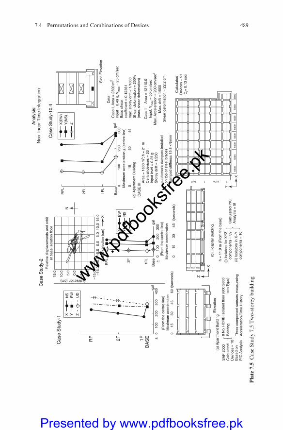
RF 2F 1F
BA
SE + –
010
020
030
040
0
015
3045
60t(
seco
nds)
015
3045
t(se
cond
s)
gal
(Fro
m th
e ce
ntre
line
)
+ –0
100
200
300
(Fro
m th
e ce
ntre
line
)
Cas
e S
tudy
-1
Cas
e S
tudy
-2
Ana
lysi
s:N
on-li
near
Tim
e In
tegr
atio
n
Cas
e S
tudy
-10.
4
–15.
0–1
5.0
–10.
0–5
.00.
0E
W d
irect
ion
(cm
)5.
010
.015
.0
–10.
0
–5.00.0
5.0
10.0
15.0
Rel
ativ
e di
spla
cem
ents
and
orb
itat
bas
e is
olat
ion
floor
lS direction (cm)
X
ZX(E
W)
Y(N
S)
RF
L
2FL
N
1FL
Bas
e 010
020
030
0
015
3045
gal
RF
L
2F 1FL
Bas
ega
l
Max
imum
acc
eler
atio
nM
axim
um a
ccel
erat
ionNS
EW
UD
Sid
e E
leva
tion
Z
X
Y
X
3900
30146299?
37503749
?8100
6200
5600
5600
5600
5600
5600
5600
5600
?? 8400
Ele
vatio
n(a
) A
part
men
t Bui
ldin
g
SA
P 2
000
Cal
cula
ted
Dev
ices
= 1
0B
ased
on
P/C
Ana
lysi
s
8 N
o. H
DR
B Is
olat
ed fl
oor
(600
280
0m
m T
ype)
h =
11.
9 m
(Fr
om th
e ba
se)
(i) Is
olat
ors
for
XY
Zco
mpo
nent
s =
39
(ii)
Isol
ator
s in
X–Y
com
pone
nts
= 1
0
Cal
cula
ted
PIC
Ana
lysi
s =
5I
Bea
ring
Thr
ee c
ompo
nent
sen
sors
mea
sure
ing
Acc
eler
atio
n-T
ime
His
tory
(b)
Hos
pita
l Bui
ldin
g
(c)
Apa
rtm
ent B
uild
ing
Dat
a:C
ase
I, A
rea
= 2
500
m2
Cas
e II
A
rea
= 1
2110
.0In
put,
Vm
ax =
50
cm/s
ecM
ax. A
ccel
erat
ion
= 2
00 c
m/s
ec2
Max
. drif
t = 1
/500
She
ar d
efor
mat
ion
= 2
2.2
cm
Cal
cula
ted
Dev
ices
= 5
1C
i=0.
13 s
ec
Inpu
t = 0
.49
g, V
max
= 2
5 cm
/sec
Bas
e sh
ear
coef
ficie
nt =
0.1
2361
max
. sto
rey
drift
< 1
/100
0S
hear
def
orm
atio
n =
200
%(m
ax. s
hear
def
orm
atio
n)C
AS
E II
I Are
a =
160
0 m
2 ; h =
21
mC
entr
al d
evic
es =
33
Inpu
t lev
el =
0.2
5 g
Sto
rey
drift
= 1
/250
elas
tom
eric
dam
pers
inst
alle
don
top
of s
teel
bra
ces
Dam
ped
stiff
ness
19.
8 kN
/mm
Max
imum
acc
eler
atio
n +_
(cen
tre
line)
X Y Z
EW NS
X Y Z
Plate
7.5
Case
Study7.5
Two-storeybuilding
7.4 Permutations and Combinations of Devices 489
www.pdfbo
oksfr
ee.pk
Presented by www.pdfbooksfree.pk
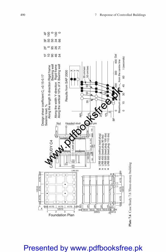
Des
ign
shea
r co
effic
ient
Ci =
0.15
-0.1
7S
eism
ic lo
ad, %
Alo
ng th
e le
ngth
X-d
irect
ion
Rig
id fr
ame
Alo
ng th
e w
idth
Y-d
irect
ion
Rig
id fr
ame
Alo
ng th
e ve
rtic
al 1
0% o
f X B
earin
g w
all
Bea
ring
wal
l
1F 10 90 46 54
2F5 95 26 74
3F 50 50 34 66
4F 100 0
100 0
1200
1200 4170
1 2 3 4
4170 417012510
1200 RF
L
4FL
3FL
2FL
1FL
GL
1200 1200
4170
4170
4170
1200
1251
0
9008203150315013420
0012
3150500 3150X
Y41
7041
7012
510
4170
1200
Foundation Plan
CA
SE
ST
UD
Y C
4
Lead
plu
g
55
100150
500700
LRB 500
150
222215
03
x 30 32
422
2215
0
712
6 x
30
LRB
450
(w
ithou
t lea
d pl
ug)
LRB
450
(le
ad p
lug
90 d
ia)
LRB
500
(le
ad p
lug
100
dia)
LRB
500
(le
ad p
lug
110
dia)
X Y Z
35 c
m/s
ec50
cm
/sec
Res
ults
from
SA
P 2
000
5050
35
35
0 015
3045
60t (
seco
nds)
BF
01F
L
2FL
3FL
4FL
RF
L
100
200
300
400
Gal
Max
imum
acc
eler
atio
n +
– fr
om th
e ce
ntre
line
Nut Headed stud Dowell pin
Plate
7.6
Case
Study7.6
Three-storeybuilding
490 7 Response of Controlled Buildings
www.pdfbo
oksfr
ee.pk
Presented by www.pdfbooksfree.pk
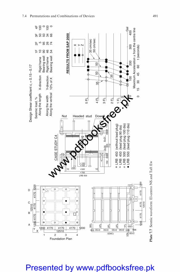
Foundation Plan
1200
4170
4170
4170
1200
1251
0
1200 4170 417012510
4170 1200
1X
Y
A
B
C
D
2 3 4
2100
9003150315031503150500 820
1200
13420
RF
L
4FL
3FL
2FL
1FL
GL
1200
4170
4170
4170
1200
1251
0
Lead
plu
g
3×30
6×31
324
712
150
150
500 1010
700
LRB 500
15055
100
Nut Headed stud Dowell pin
22
22
22
22
RE
SU
LTS
FR
OM
SA
P 2
000
5 F
L
X Y Z
4 F
L
3 F
L
3550
35
50
35 c
m/s
ec50
cm
/sec
2 F
L
1 F
L
BF
00
100
200
300
400G
al
0
15
3
0
45
6
0
t (
seco
nds)
M
axim
um A
ccel
erat
ion
± fr
om th
e ce
ntre
line
Sei
smic
load
, %
A
long
the
leng
th
Alo
ng th
e w
idth
A
long
the
vert
ical
1F 10 90 46 54
2F5 95 26 74
3F 50 50 34 66
4F 100 0
100 0
X-d
irect
ion
Y-di
rect
ion
10%
of X
Rig
id fr
ame
Bea
ring
wal
lR
igid
fram
eB
earin
g w
all
CA
SE
ST
UD
Y C
4
Des
ign
She
ar c
oeffi
cien
t ci =
0.1
5 –
0.17
LRB
450
(w
ithou
t lea
d pl
ug)
LRB
450
(le
ad p
lug
90 d
ia)
LRB
500
(le
ad p
lug
100
dia)
LRB
550
(le
ad p
lug
110
dia)
Plate
7.7
Sesmicwaveform
:El-centroNSandTaftEw
7.4 Permutations and Combinations of Devices 491
www.pdfbo
oksfr
ee.pk
Presented by www.pdfbooksfree.pk
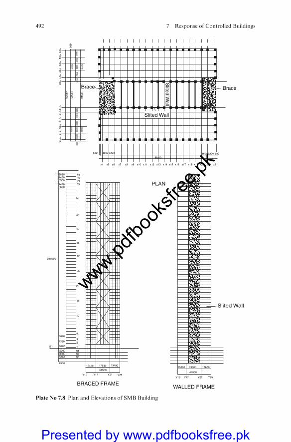
Slited Wall
PLAN
15600 13300 15600
44500
Y13 Y17 Y21 Y25
WALLED FRAMEBRACED FRAME
55
50
45
40
35
30
25
20
15
10
1
23
5
P1P2P3
3690
7360
5200
5200
250013400 17540 13480
44500
36003600
B1
G1
B2B3
Y13 Y17 Y21 Y25
210200
385044506500
44803690
Brace Brace
Slited W
all
680
36003200
32003480
2120
13300
23203480
32003200
3600
13400
15600
600
17540
44500
13440
15600
Y25
Y24
Y23
Y22
Y21
Y20
Y18
Y17
Y16
Y15
Y14
Y13
680 3600 3200
x4 x5 x6 x7 x8 x9 x10 x11 x12 x13 x14 x15 x16 x17 x18 x19 x20 x21 x21
68032003600
58.00
Slited Wall
Plate No 7.8 Plan and Elevations of SMB Building
492 7 Response of Controlled Buildings
www.pdfbo
oksfr
ee.pk
Presented by www.pdfbooksfree.pk

7.4 Permutations and Combinations of Devices 493
www.pdfbo
oksfr
ee.pk
Presented by www.pdfbooksfree.pk

Case Study 7.5 Obayashi-Gumi Technical Research Center LaboratoryDesigned by Obayashi-Gumi Ltd, Tokyo, Japan
Building Data: - Reinforced concrete rigid frame building with RCC aseismic
wall
– Total floor area: 1623.89 m2; total height=22.80 m=h (m)– Area/floor=328.75 m2
– Type of earthquake waveform: El-Centro with accelerations amplitude300–400 cm/s2
– Total floors: 5 above ground, 1 penthouse– Dampers: 24 nos in sets of 4 are positioned. Total no. = 96– Isolators: 14 nos are positioned
with A, B, C, D permutation and combinationThe total number computed = 98
Soil Property and Foundation Data
Note: These data are used for soil–structure interaction analysis
Ground propertyFoundation depthPHC file
FormationGL-1.775 m Piledepth FormationGL-7.0 m
Soil property and N value
GL-m 0–0.7 m 0.7–6.2 m >6.2 m
Soil type Red Loam Loam Gravel
N value: – 2–3 >50
Permissible pile resistance PHC pile (Type A, B) cement grouting method (methodapproved by Ministry of Construction under Section 38 ofits regulations)
45 dia 66 t/pile (long time); 132 t/pile (short term)
Case Study 7.6 A Comparative Study of ResultsAnalysis type: Seismic Waveform type Degree of FreedomFinite element Three-Dimensional El-Centro 300–345 gal 6/floor
S.No. Obayashi-Gumi Ltd, Tokyo, Japan Program ISOPAR and Graph G-typeDIRECTION DirectionType X* Y* Z* X* Y* Z*
1 Fundamental period (s)(a) mode 1 3.12 3.08 – 2.92 3.01 1.05(b) mode 2 0.42 0.25 – 0.39 0.22 0.01
2 Damping constant(x & b)
0.02 0.01 – 0.015 25 cm/s 0.02 50 m/s 0.001
3 Shear coefficientCi building
0.122 (F1)Input25 cm/s
0.120 (F1) – 0.119 (F1) 0.119 (F1) 0.100
494 7 Response of Controlled Buildings
www.pdfbo
oksfr
ee.pk
Presented by www.pdfbooksfree.pk
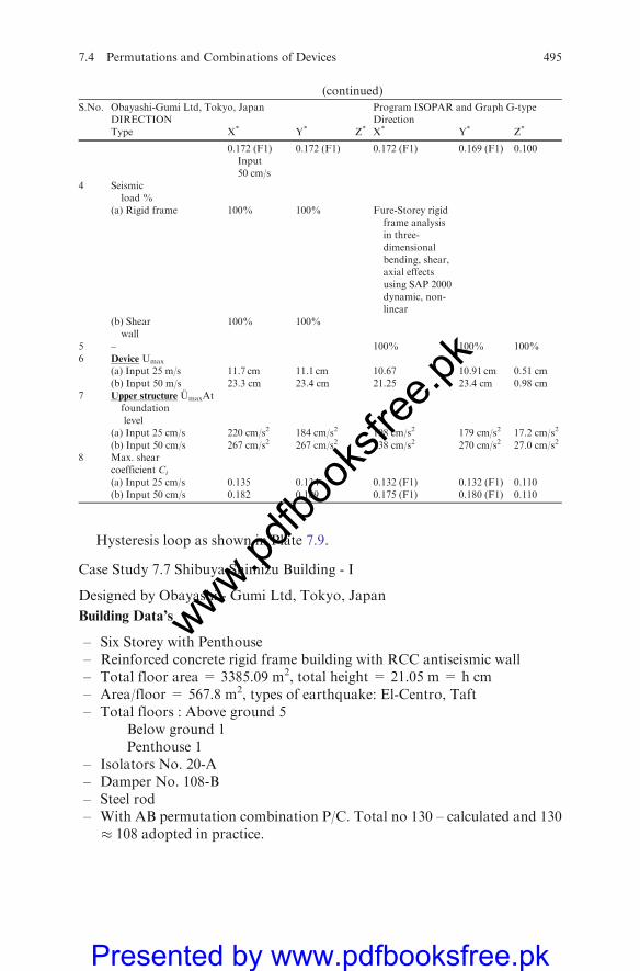
(continued)
S.No. Obayashi-Gumi Ltd, Tokyo, Japan Program ISOPAR and Graph G-typeDIRECTION DirectionType X* Y* Z* X* Y* Z*
0.172 (F1)Input50 cm/s
0.172 (F1) 0.172 (F1) 0.169 (F1) 0.100
4 Seismicload %
(a) Rigid frame 100% 100% Fure-Storey rigidframe analysisin three-dimensionalbending, shear,axial effectsusing SAP 2000dynamic, non-linear
(b) Shearwall
100% 100%
5 – 100% 100% 100%6 Device Umax
(a) Input 25 m/s 11.7 cm 11.1 cm 10.67 10.91 cm 0.51 cm(b) Input 50 m/s 23.3 cm 23.4 cm 21.25 23.4 cm 0.98 cm
7 Upper structure UmaxAtfoundationlevel
(a) Input 25 cm/s 220 cm/s2 184 cm/s2 198 cm/s2 179 cm/s2 17.2 cm/s2
(b) Input 50 cm/s 267 cm/s2 267 cm/s2 238 cm/s2 270 cm/s2 27.0 cm/s2
8 Max. shearcoefficient Ci
(a) Input 25 cm/s 0.135 0.134 0.132 (F1) 0.132 (F1) 0.110(b) Input 50 cm/s 0.182 0.189 0.175 (F1) 0.180 (F1) 0.110
Hysteresis loop as shown in Plate 7.9.
Case Study 7.7 Shibuya Shimizu Building - I
Designed by Obayashi - Gumi Ltd, Tokyo, Japan
Building Data’s
– Six Storey with Penthouse– Reinforced concrete rigid frame building with RCC antiseismic wall– Total floor area = 3385.09 m2, total height = 21.05 m = h cm– Area/floor = 567.8 m2, types of earthquake: El-Centro, Taft– Total floors : Above ground 5
Below ground 1Penthouse 1
– Isolators No. 20-A– Damper No. 108-B– Steel rod– With AB permutation combination P/C. Total no 130 – calculated and 130� 108 adopted in practice.
7.4 Permutations and Combinations of Devices 495
www.pdfbo
oksfr
ee.pk
Presented by www.pdfbooksfree.pk
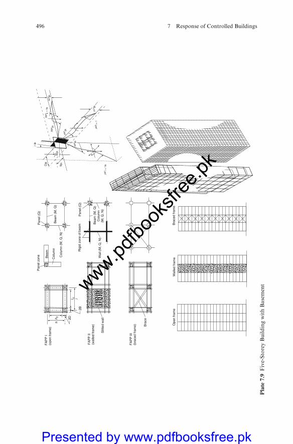
2B
I c i
2D
hh 0
Col
umn
Bea
m
Pan
el z
one
Pan
el (
Q)
Pan
el (
Q)
Col
umn
(M, Q
, N)
Col
umn
(M, Q
, N)
Wal
l (M
, Q, N
)
Rig
id z
one
of b
eam
Bea
m (
M, Q
)
Bea
m (
M, Q
)
Slit
ted
wal
l
FA
PP
II(w
alle
d fr
ame)
FA
PP
III
(bra
ced
fram
e)
FA
PP
I(o
pen
fram
e)
Bra
ce
Ope
n fr
ame
Wal
led
fram
eB
race
d fr
ame
i +
1ikU
ijk
Vijk
Wijk
ijk
γ
ijk
Xθg
ijk
yθ9
ij 1
kX
θ9+
ijk
yλ9
i +
1yθ
9
yθc
ijk
xθ0
ijk
xy9
Plate
7.9
Five-StoreyBuildingwithBasement
496 7 Response of Controlled Buildings
www.pdfbo
oksfr
ee.pk
Presented by www.pdfbooksfree.pk
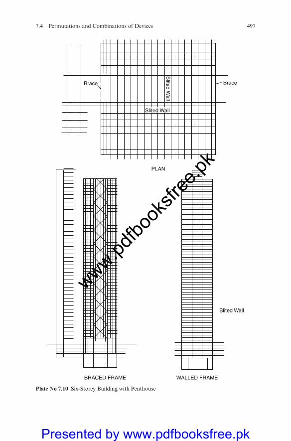
Slited Wall
BRACED FRAME WALLED FRAME
PLAN
Brace Brace
Slited W
all
Slited Wall
Plate No 7.10 Six-Storey Building with Penthouse
7.4 Permutations and Combinations of Devices 497
www.pdfbo
oksfr
ee.pk
Presented by www.pdfbooksfree.pk

Soil Property and Foundation Data
For Soil–Structural InteractionNote: These data are used for soil–structural interaction analysis
GL-m 0–1.0 1.0–6.7 6.7–10.4 10.4–13.2 13.2–15.4 15.4–18.7 18.7–20.0 20.0–25.4 25.4–30.2
Soil Redloam
Loam Clayloam
TuffClay
Sandysilt
Silt Very finesand
Gravel Clay
Nvalue – 4–23 3–6 8 4–5 5–8 23 50 >50
Permissible pile Cast in situ concrete pile (earth drill method): Long termResistance 160 t/pile 1,200 dia 280 t/pile
Outline of the Structure
Foundation
Ground type and Pile foundation: Cast in-situ pile supported directly onfoundation structure gravel layer at GL-20.0 mMaximum contact pressure Cast in situ concrete pile.(pile resistance) 900 dia at 1,200 dia at 1,200 dia at
side column middle column corner columnLong term156 t/pile 235 t/pile 264 t/pileShort term199 t/pile 261 t/pile 382 t/pile
Main structure
Structural features It is a menhin structure where the menhin device is placedbetween the RCC upper structure and the foundation
Frame classification Along the length: RCC rigid frameAlong the width: RCC antiseismic wall
Bearing wall, other wallsmaterials for columns
Column – B � D = 400 � 450, 450 � 450, 500 � 500, 450 �350
Beams, sections Beams – B � D = 220 � 750, 220 – 250 � 1050, 220 – 250 �1,150, 250 � 400; Steel bars – deformed bars SD35 (JIS G3,112); concrete – FC = 210 kg/cm2 (for foundation andfoundation beam)
Columns, beams, joints RCC rigid structureFloor Cast in situ RCC structureRoof Cast in situ flat slab structureNon-bearing walls Outer wall – ALC plate; Inner wall – ALC plateFire-proof coating
Structural Design
Laminated rubber (20 nos) 100–150 ton (8 nos). Each consists of rubber – natural rubber5 thick � 620 dia (50 layers); steel plate; insertion plate –SS41 (JIS G 3101); flange plate – SS41 (JIS G 3101); 20–28� 830 dia (top and bottom); fixing bolt – high-tension boltFBT (JIS B 1186) M24
200–250 ton (12 nos). Each consists of Rubber – naturalrubber 6 thick � 740 dia (45 layers); steel plate: insertionplate SS41 (JIS G 3101) 3.1� 740 dia (44 Nos); flange plate– SS41 (JIS G 3101) 24–30 � 985 dia (top and bottom);fixing bolt – High-tension bolt FBT (JIS B 1186) M24.
Rubber properties:Rubber hardness: 40 � 525% shear modulus (kg/cm2): 3.4 � 1.0
498 7 Response of Controlled Buildings
www.pdfbo
oksfr
ee.pk
Presented by www.pdfbooksfree.pk
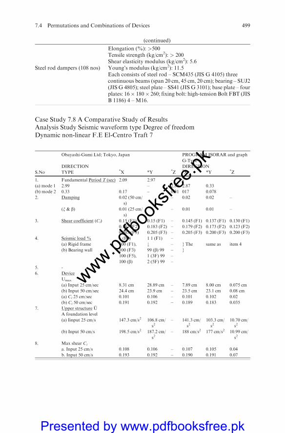
(continued)
Elongation (%): >500Tensile strength (kg/cm2): > 200Shear elasticity modulus (kg/cm2): 5.6
Steel rod dampers (108 nos) Young’s modulus (kg/cm2): 11.5Each consists of steel rod – SCM435 (JIS G 4105) threecontinuous beams (span 20 cm, 45 cm, 20 cm); bearing – SUJ2(JIS G 4805); steel plate – SS41 (JIS G 3101); base plate – fourplates: 16� 180� 260; fixing bolt: high-tension Bolt FBT (JISB 1186) 4 – M16.
Case Study 7.8 A Comparative Study of ResultsAnalysis Study Seismic waveform type Degree of freedomDynamic non-linear F.E El-Centro Traft 7
Obayashi-Gumi Ltd; Tokyo, Japan PROGRAM ISORAR and graph
G-Type
DIRECTION DIRECTION
S.No TYPE *X *Y *Z *X *Y *Z
1. Fundamental Period T (sec) 2.09 2.97 – -
(a) mode 1 2.99 – 2.89 2.87 0.33
(b) mode 2 0.33 0.17 – 0.31 017 0.078
2. Damping 0.02 (50 cm/
s)
– 0.02 0.02 –
(x & b) 0.01 (25 cm/
s)
– 0.01 0.01 –
3. Shear coefficient (Ci) 0.15 (F1) 0.15 (F1) – 0.145 (F1) 0.137 (F1) 0.130 (F1)
0.183 (F2) 0.183 (F2) – 0.179 (F2) 0.173 (F2) 0.123 (F2)
0.205 (F3) 0.205 (F3) – 0.205 (F3) 0.200 (F3) 0.200 (F3)
4. Seismic load % – (F2) 1 1 (F1) –
(a) Rigid frame 100 (F1), # – } The same as item 4
(b) Bearing wall 100 (F3) 99 (b) 99 – }
100 (F5), 1 (3F) 99 –
100 (b) 2 (5F) 99 –
5. -
6. Device
Umax
(a) Input 25 cm/sec 8.31 cm 28.89 cm – 7.89 cm 8.00 cm 0.075 cm
(b) Input 50 cm/sec 24.4 cm 23.9 cm – 23.5 cm 23.1 cm 0.08 cm
(a) Ci 25 cm/sec 0.101 0.106 – 0.101 0.102 0.02
(b) Ci 50 cm/sec 0.191 0.192 – 0.189 0.183 0.035
7. Upper structure U
A foundation level
(a) Iinput 25 cm/s 147.3 cm/s2 106.8 cm/
s2– 141.3 cm/
s2103.3 cm/
s210.70 cm/
s2
(b) Input 50 cm/s 198.5 cm/s2 187.2 cm/
s2– 188 cm/s2 177 cm/s2 10.99 cm/
s2
8. Max shear Ci
a. Input 25 cm/s 0.108 0.106 – 0.107 0.105 0.04
b. Input 50 cm/s 0.193 0.192 – 0.190 0.191 0.07
7.4 Permutations and Combinations of Devices 499
www.pdfbo
oksfr
ee.pk
Presented by www.pdfbooksfree.pk
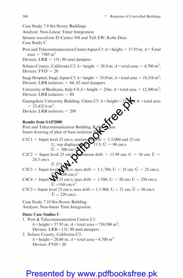
Case Study 7.9 Six-Storey Buildings
Analysis: Non-Linear Timer Integration
Seismic waveform El-Centro NS and Taft EW; Kobe DataCase Study C
Post and Telecommunication Center Japan C1: h=height= 37.95m;A=Total
area = 7305 m2
Devices: LRB = 131; 90 steel dampers
Solano County, California C2: h=height = 28.0 m; A=total area = 4,700 m2;Devices: FVD = 20
Inagi Hospital, Inagi, Japan C3: h=height= 35.81m;A=total area= 18,518m2;Devices: LRB isolators = 84; 42 steel dampers
University of Basilicata, Italy C4: h=height = 25m;A=total area= 12,500 m2;Devices: LRB isolators = 80
Guangzhou University Building, China C5: h=height=22.5 m; A=total area
= 23,452.6 m2;Devices: LRB isolators = 209
Results from SAP2000
Post and Telecommunication Building, Kobe, JapanInsert drawing of plan of base isolation floor.
C1C1 = Input level 25 cm/s; maximum drift = 1/5,000 and 25 cmU, top displacement = 13.5; U = 90 cm/sU = 300 cm/s2
C2C2 = Input level 25 cm/s; maximum drift = 13.98 cm; U = 36 cm; U =24.5 cm/s
U 375 cm/s2
C3C3 = Input level 50 cm/s; max drift = 1/1,780; U = 35 cm; U = 25 cm/s;U = 200 cm/s2
C4C4 = Input level 25 cm/s; max drift = 1/500; U = 20 cm; U ¼ 250 cm/s;U ¼168 cm/s2
C5C5 ¼ Input level 25 cm/s; max drift ¼ 1/1,906; U ¼ 21 cm; U ¼ 30 cm/sU ¼ 220 cm/s
Case Study 7.10 Six-Storey BuildingAnalysis: Non-linear Time Integration
Data: Case Studies C
1. Post & Telecommunication Centre C1:h=height=37.95 m; A=total area=730,500 m2;Devices: LRB=131; 90 steel dampers
2. Solano County, California C2:h=height=28.00 m; A=total area=4,700 m2
Devices: FVD=20
500 7 Response of Controlled Buildings
www.pdfbo
oksfr
ee.pk
Presented by www.pdfbooksfree.pk
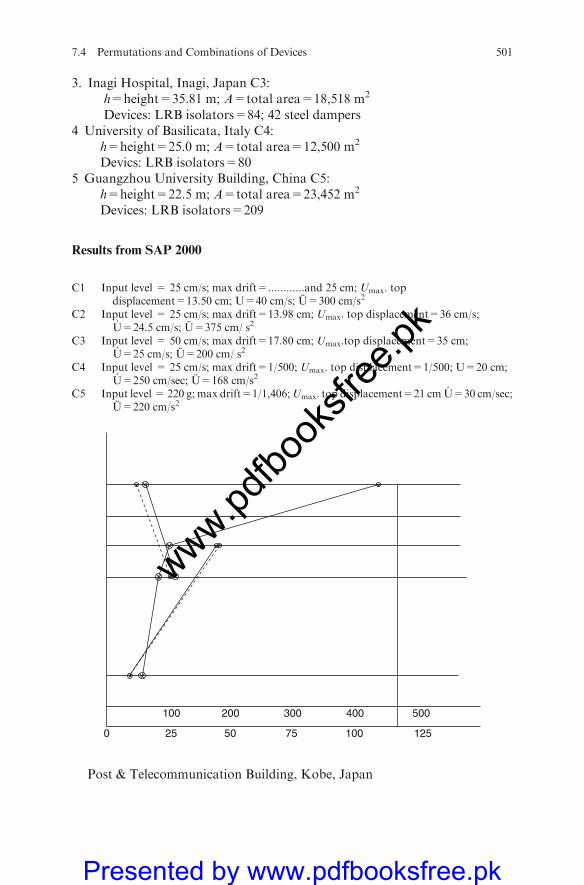
3. Inagi Hospital, Inagi, Japan C3:h=height=35.81 m; A=total area=18,518 m2
Devices: LRB isolators=84; 42 steel dampers4 University of Basilicata, Italy C4:
h=height=25.0 m; A=total area=12,500 m2
Devics: LRB isolators=805 Guangzhou University Building, China C5:
h=height=22.5 m; A=total area=23,452 m2
Devices: LRB isolators=209
Results from SAP 2000
C1 Input level = 25 cm/s; max drift=............and 25 cm; Umax. topdisplacement=13.50 cm; U=40 cm/s; U=300 cm/s2
C2 Input level = 25 cm/s; max drift=13.98 cm; Umax. top displacement=36 cm/s;U=24.5 cm/s; U=375 cm/ s2
C3 Input level = 50 cm/s; max drift=17.80 cm; Umax.top displacement=35 cm;U=25 cm/s; U=200 cm/ s2
C4 Input level = 25 cm/s; max drift=1/500; Umax. top displacement=1/500; U=20 cm;U=250 cm/sec; U=168 cm/s2
C5 Input level= 220 g; max drift=1/1,406;Umax. top displacement=21 cm U=30 cm/sec;U=220 cm/s2
Post & Telecommunication Building, Kobe, Japan
0 25 50 75 100 125
100 200 300 400 500
7.4 Permutations and Combinations of Devices 501
www.pdfbo
oksfr
ee.pk
Presented by www.pdfbooksfree.pk

Case Study 7.11 Seven-Storey BuildingSeismic WaveForm : El-Centro NS and TAFT, EWDATA: CASE STUDY C
Insert floor plan drawing?System Plaza Isogo, C1: h=height = 30.3 m; A=total area = 9,242.13 m2
Yokohama city, Japan Devices: Isolators = 24; devices computed = 58Dampers = 28Lead steel 52 Adopted
Yinhe Building C2: h=height = 18.9 m; A=total area = 130,000 m2
Wulumugi city,China Devices: LRB isolators = 123; Adopted 206Dampers = 86Devices computed P/CLRB + dampers = 200
RESULTS: SAP2000C1 Input level = 50 cm/s; storey drift = 1/200U = 39 cm/s; U= 50 cm/s; U= 264 cm/s2
C2 Input level = 400 gal; storey drift = 22 cmU = 50 cm/s; U = 400 cm/s2; Ci = 0.21
Insert graph from excel?
502 7 Response of Controlled Buildings
www.pdfbo
oksfr
ee.pk
Presented by www.pdfbooksfree.pk
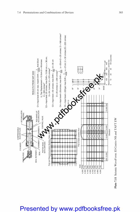
Pos
t and
Tel
ecom
mun
icat
ion
Bui
ldin
g, K
obe
JAPA
N
PIS
TON
RO
D
CY
LIN
DE
R
PIS
TON
HE
AD
WIT
H O
RF
ICE
S
SE
AL
RE
TAIN
ER
SE
AL
CH
AM
BE
R 1
CH
AM
BE
R 2
CO
NT
RO
L V
ALV
E
RO
D M
AK
E-U
PA
CC
UM
ULA
TOR
AC
CU
MU
LATO
RH
OU
SIN
G
CO
MP
RE
SS
IBLE
SIL
ICO
N F
LUID
Ele
vatio
nM
axim
um a
ccel
erat
ion
+ c
entr
al li
ne
4.20
0
PH
RP
lan
of b
ase
isol
atio
n flo
or
000
12.0
0012
.000
12.0
0012
.000
000
PH
2
7EL
6EL
5EL
4EL
3EL
2EL
1EL
5.30
0
4.15
0
4.35
0
4.75
0
4.25
0
4.75
0
5.80
0
5F6F 4F 3F 2F 1F
0 010
2030
t (se
cond
s)40
100
200
300
400ga
lB
AS
E
x y z
RE
SU
LTS
FR
OM
SA
P 2
000
C1=
Inpu
t lev
el 2
5 cm
/sec
; max
im-D
rift
=1
5000
And
25
cm
U_T
op D
ispl
acem
ent =
13.5
cm;Ú
= 4
0cm
/sec
Ü =
300
cm
/sec
2
Ú =
25
cm/s
ec; ü
= 2
00 c
m/s
ec2
Ú =
24.
5 c
m/s
ec; U
= 3
75 c
m/s
ec2
C2
= In
put l
evel
: 25
cm
/sec
; max
.Drif
t = 1
3.98
cm
; u =
36
cm;
; U =
35
cm
C3
= In
put l
evel
= 5
0 c
m/s
ec; m
ax.D
rift =
1 780
C5
= In
put l
evel
= 2
20 g
al; m
ax.D
rift =
; u =
21
cm; Ú
= 3
0 c
m/s
ec;Z
Ü =
220
cm
/sec
114
06
C4
= In
put l
evel
= 2
5cm
/sec
; max
Drif
t =1 500
;u =
20
cm Ú
= 2
5 cm
/sec
; Ü =
168
cm
/sec
2
CA
SE
ST
UD
Y C
I
Plate
7.11Seism
icWaveF
orm
:El-CentroNSandTAFTEW
7.4 Permutations and Combinations of Devices 503
www.pdfbo
oksfr
ee.pk
Presented by www.pdfbooksfree.pk

1.0 × 10⁵ t.m
DISPLACEMENT STOREY SHEAR
Response - IV
OVER TURNING MOMENT
2000 t6.40 sec 6.40 sec 6.40 sec
Animated earthquake response 4
ENLARGEDBY
50 TIMES
0.40 cm
–4000 4000SHEAR
0
–4000 4000SHEAR
0
–4000 4000SHEAR
0
–4000 4000SHEAR
0
–4000 4000SHEAR
0
–3.0 0 3.0OVTM
×105
–3.0 0 3.0OVTM
×105
–3.0 0 3.0OVTM
×105
–3.0 0 3.0OVTM
×105
–3.0 0 3.0OVTM
×105
1.0 × 10⁵ t.m2000 t6.80 sec 6.80 sec 6.80 sec
1.0 × 10⁵ t.m2000 t7.20 sec
7.20 sec 7.20 sec
1.0 × 10⁵ t.m2000 t7.60 sec 7.60 sec 7.60 sec
1.0 × 10⁵ t.m2000 t8.00 sec 7.60 sec 7.60 sec
ENLARGEDBY
50 TIMES
0.40 cm
ENLARGEDBY
50 TIMES
0.40 cm
ENLARGEDBY
50 TIMES
0.40 cm
ENLARGEDBY
50 TIMES
0.40 cm
Plate 7.12
504 7 Response of Controlled Buildings
www.pdfbo
oksfr
ee.pk
Presented by www.pdfbooksfree.pk
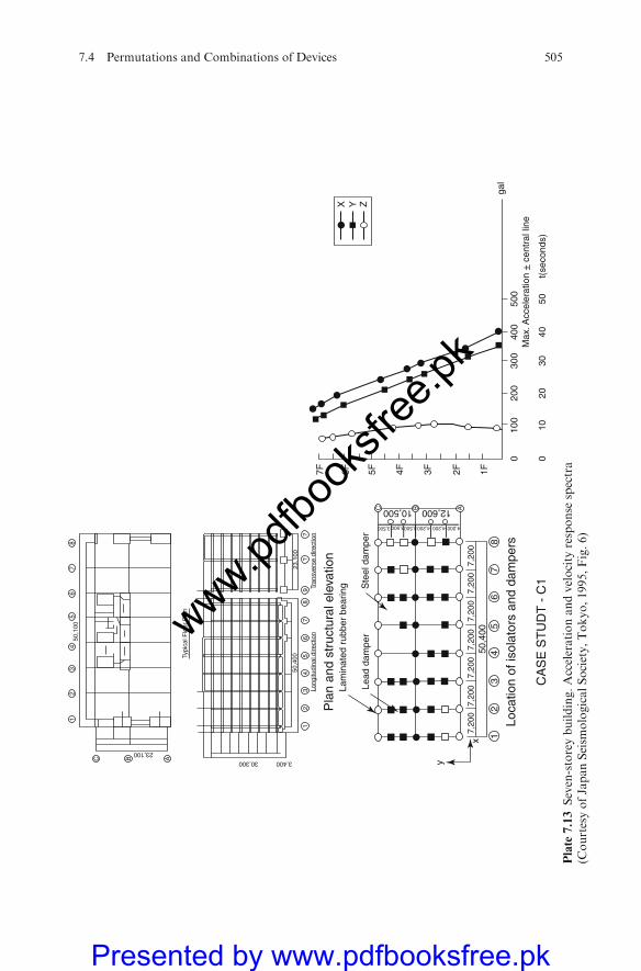
12
34
550
,400
12,600
4,2004,200
7,20
07,
200
7,20
07,
200
7,20
07,
200
7,20
0
4,2003,5003,5003,500
10,500
67
8
Loca
tion
of is
olat
ors
and
dam
pers
CA
SE
ST
UD
T -
C1Ste
el d
ampe
rLe
ad d
ampe
r
Lam
inat
ed r
ubbe
r be
arin
gP
lan
and
stru
ctur
al e
leva
tion
y
x
50,4
00
23,100
30,300 3,400
50,1
00
23,1
00
C B A
1Lo
ngitu
dina
l dire
ctio
nTr
ansv
erse
dire
ctio
n2
34
56
78
9?
?
C B A
12
34
56
78
Typi
cal F
loor
Pla
n
0
1F2F3F4F5F6F7F
100
200
300
400
500
010
2030
4050
Max
. Acc
eler
atio
n + –
cen
tral
line
t(se
cond
s)
gal
X Y Z
Plate
7.13Seven-storeybuilding.Accelerationandvelocity
response
spectra
(CourtesyofJapanSeism
ologicalSociety,Tokyo,1995,Fig.6)
7.4 Permutations and Combinations of Devices 505
www.pdfbo
oksfr
ee.pk
Presented by www.pdfbooksfree.pk

RF 2F 1F
BA
SE + –
010
020
030
040
0
015
3045
60t(
seco
nds)
015
3045
t(se
cond
s)
gal
(Fro
m th
e ce
ntre
line
)
+ –0
100
200
300
(Fro
m th
e ce
ntre
line
)
Cas
e S
tudy
-1
Cas
e S
tudy
-2
Ana
lysi
s:N
on-li
near
Tim
e In
tegr
atio
n
Cas
e S
tudy
-10.
4
–15.
0–1
5.0
–10.
0–5
.00.
0E
W d
irect
ion
(cm
)5.
010
.015
.0
–10.
0
–5.00.0
5.0
10.0
15.0
Rel
ativ
e di
spla
cem
ents
and
orb
itat
bas
e is
olat
ion
floor
lS direction (cm)
X
ZX(E
W)
Y(N
S)
RF
L
2FL
N
1FL
Bas
e 010
020
030
0
015
3045
gal
RF
L
2F 1FL
Bas
ega
l
Max
imum
acc
eler
atio
nM
axim
um a
ccel
erat
ionNS
EW
UD
Sid
e E
leva
tion
Z
X
Y
X
3900
30146299?
37503749
?8100
6200
5600
5600
5600
5600
5600
5600
5600
?? 8400
Ele
vatio
n(a
) A
part
men
t Bui
ldin
g
SA
P 2
000
Cal
cula
ted
Dev
ices
= 1
0B
ased
on
P/C
Ana
lysi
s
8 N
o. H
DR
B Is
olat
ed fl
oor
(600
280
0m
m T
ype)
h =
11.
9 m
(Fr
om th
e ba
se)
(i) Is
olat
ors
for
XY
Zco
mpo
nent
s =
39
(ii)
Isol
ator
s in
X–Y
com
pone
nts
= 1
0
Cal
cula
ted
PIC
Ana
lysi
s =
5I
Bea
ring
Thr
ee c
ompo
nent
sen
sors
mea
sure
ing
Acc
eler
atio
n-T
ime
His
tory
(b)
Hos
pita
l Bui
ldin
g
(c)
Apa
rtm
ent B
uild
ing
Dat
a:C
ase
I, A
rea
= 2
500
m2
Cas
e II
A
rea
= 1
2110
.0In
put,
Vm
ax =
50
cm/s
ecM
ax. A
ccel
erat
ion
= 2
00 c
m/s
ec2
Max
. drif
t = 1
/500
She
ar d
efor
mat
ion
= 2
2.2
cm
Cal
cula
ted
Dev
ices
= 5
1C
i=0.
13 s
ec
Inpu
t = 0
.49
g, V
max
= 2
5 cm
/sec
Bas
e sh
ear
coef
ficie
nt =
0.1
2361
max
. sto
rey
drift
< 1
/100
0S
hear
def
orm
atio
n =
200
%(m
ax. s
hear
def
orm
atio
n)C
AS
E II
I Are
a =
160
0 m
2 ; h =
21
mC
entr
al d
evic
es =
33
Inpu
t lev
el =
0.2
5 g
Sto
rey
drift
= 1
/250
elas
tom
eric
dam
pers
inst
alle
don
top
of s
teel
bra
ces
Dam
ped
stiff
ness
19.
8 kN
/mm
Max
imum
acc
eler
atio
n +_
(cen
tre
line)
X Y Z
EW NS
X Y Z
Plate
No7.14
Eight-storeybuildings
506 7 Response of Controlled Buildings
www.pdfbo
oksfr
ee.pk
Presented by www.pdfbooksfree.pk

1.0 × 10⁵ t.m
DISPLACEMENT STOREY SHEAR
Response - IV
OVER TURNING MOMENT
2000 t6.40 sec 6.40 sec 6.40 sec
Animated earthquake response 4
ENLARGEDBY
50 TIMES
0.40 cm
–4000 4000SHEAR
0
–4000 4000SHEAR
0
–4000 4000SHEAR
0
–4000 4000SHEAR
0
–4000 4000SHEAR
0
–3.0 0 3.0OVTM
×105
–3.0 0 3.0OVTM
×105
–3.0 0 3.0OVTM
×105
–3.0 0 3.0OVTM
×105
–3.0 0 3.0OVTM
×105
1.0 × 10⁵ t.m2000 t6.80 sec 6.80 sec 6.80 sec
1.0 × 10⁵ t.m2000 t7.20 sec
7.20 sec 7.20 sec
1.0 × 10⁵ t.m2000 t7.60 sec 7.60 sec 7.60 sec
1.0 × 10⁵ t.m2000 t8.00 sec 7.60 sec 7.60 sec
ENLARGEDBY
50 TIMES
0.40 cm
ENLARGEDBY
50 TIMES
0.40 cm
ENLARGEDBY
50 TIMES
0.40 cm
ENLARGEDBY
50 TIMES
0.40 cm
Plate No 7.15
7.4 Permutations and Combinations of Devices 507
www.pdfbo
oksfr
ee.pk
Presented by www.pdfbooksfree.pk
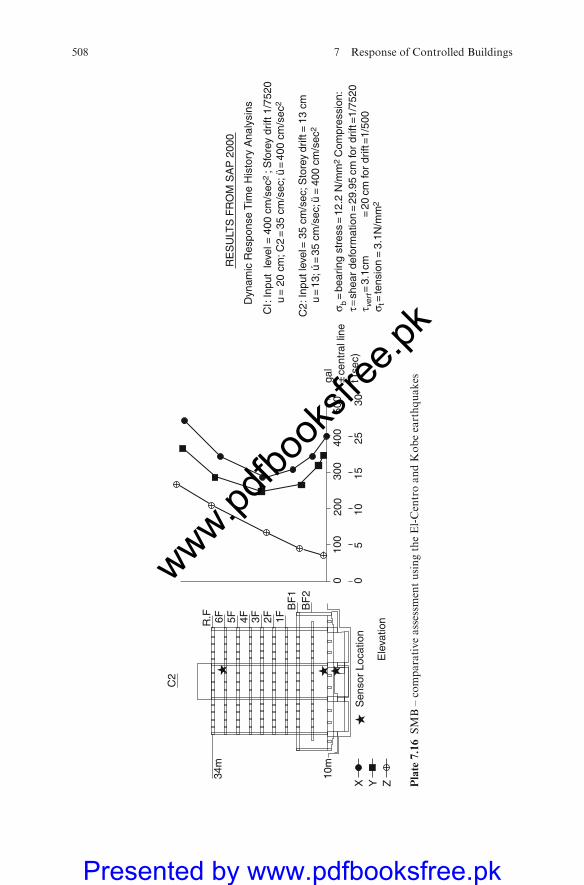
200
100
0
1015
50
2530
300
400
500
X Y Z
gal
± c
entr
al li
net (
sec)
Sen
sor
Loca
tion
Ele
vatio
n
C2
R.F 6F 5F 4F 3F 2F 1F
BF
1B
F2
34m
10m
RE
SU
LTS
FR
OM
SA
P 2
000
: Inp
ut l
evel
= 4
00 c
m/s
ec2
; Sfo
rey
drift
1/7
520
u =
20
cm; C
2 =
35
cm/s
ec; ü
= 4
00 c
m/s
ec2
: Inp
ut le
vel =
35
cm/s
ec; S
tore
y dr
ift =
13
cmu
= 1
3; ú
= 3
5 cm
/sec
; ü =
400
cm
/sec
2
σ b = b
earin
g st
ress
= 1
2.2
N/m
m2
Com
pres
sion
:τ =
shea
r de
form
atio
n =
29.9
5 cm
for
drift
=1/
7520
τ ver
t = 3
.1cm
= 2
0 cm
for
drift
=1/
500
σ t =
tens
ion
= 3.
1N/m
m2
Dyn
amic
Res
pons
e T
ime
His
tory
Ana
lysi
ns
CI
C2
Plate
7.16SMB–comparativeassessm
entusingtheEl-CentroandKobeearthquakes
508 7 Response of Controlled Buildings
www.pdfbo
oksfr
ee.pk
Presented by www.pdfbooksfree.pk
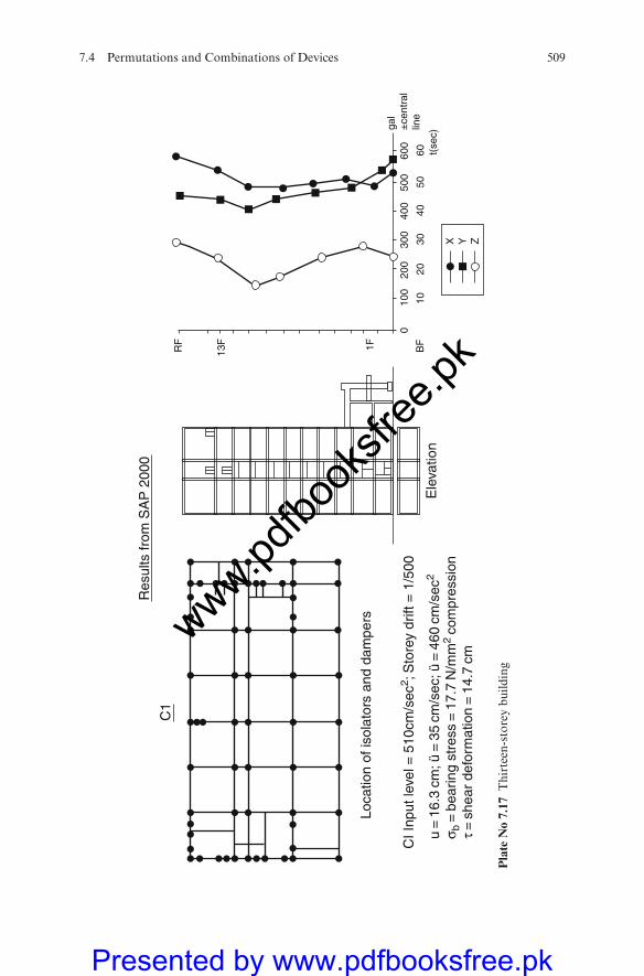
Loca
tion
of is
olat
ors
and
dam
pers
CI I
nput
leve
l = 5
10cm
/sec
2 ; S
tore
y dr
ift =
1/5
00
u =
16.
3 cm
; ü =
35
cm/s
ec; ü
= 4
60 c
m/s
ec2
σ b =
bea
ring
stre
ss =
17.
7 N
/mm
2 co
mpr
essi
onτ =
she
ar d
efor
mat
ion
= 1
4.7
cm
Res
ults
from
SA
P 2
000
C1
0
BF
Ele
vatio
n10
2030
4050
60 t(se
c)
100
200
300
400
500
600
gal
±ce
ntra
llin
e
RF
13F 1F
X Y Z
Plate
No7.17Thirteen-storeybuilding
7.4 Permutations and Combinations of Devices 509
www.pdfbo
oksfr
ee.pk
Presented by www.pdfbooksfree.pk
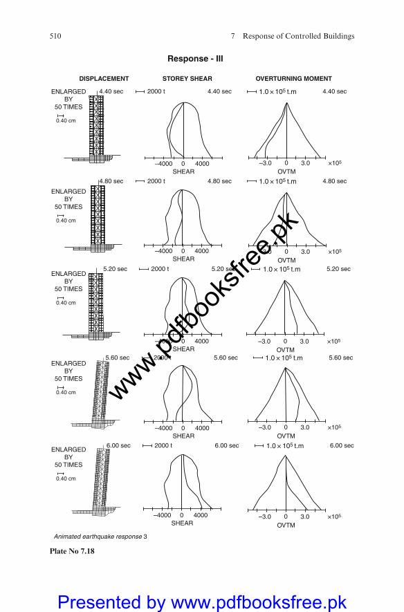
1.0 × 10⁵ t.m
DISPLACEMENT STOREY SHEAR
Response - III
OVERTURNING MOMENT
2000 t4.40 sec 4.40 sec 4.40 sec
Animated earthquake response 3
ENLARGEDBY
50 TIMES
0.40 cm
–4000 4000SHEAR
0
–4000 4000SHEAR
0
–4000 4000SHEAR
0
–4000 4000SHEAR
0
–4000 4000SHEAR
0
–3.0 0 3.0OVTM
×105
–3.0 0 3.0OVTM
×105
–3.0 0 3.0OVTM
×105
–3.0 0 3.0OVTM
×105
–3.0 0 3.0OVTM
×105
ENLARGEDBY
50 TIMES
0.40 cm
ENLARGEDBY
50 TIMES
0.40 cm
ENLARGEDBY
50 TIMES
0.40 cm
ENLARGEDBY
50 TIMES
0.40 cm
1.0 × 10⁵ t.m2000 t4.80 sec 4.80 sec 4.80 sec
1.0 × 10⁵ t.m2000 t5.20 sec 5.20 sec 5.20 sec
1.0 × 10⁵ t.m2000 t5.60 sec 5.60 sec 5.60 sec
1.0 × 10⁵ t.m2000 t6.00 sec 6.00 sec 6.00 sec
Plate No 7.18
510 7 Response of Controlled Buildings
www.pdfbo
oksfr
ee.pk
Presented by www.pdfbooksfree.pk
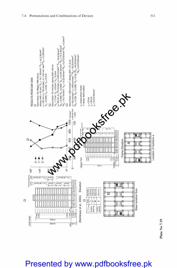
CI
C2
CI
Not
e
Rub
ber
Bea
ring
Slid
ing
Bea
ring
Dia
met
er
1100
mm
1100
mm
1200
mm
1300
mm
CI
18F
14F 9F 4F 1F
200
5010
00
400
600
800
1000
X Y Z
150
mm
/sec
2
+ c
entr
al li
net (
sec)
(Nis
hika
wa
et a
l., 2
004)
Bas
e is
olat
ion
floor
Loca
tion
of Is
olat
ors
a
Ele
vatio
n
Fram
e E
leva
tion
Tota
l Hei
ght
Col
umns
,Jo
ints
Bea
ms,
Sla
b
4,08
03,
950
Fc = 36 N/mm2
Fc = 48 N/mm2Fc = 36 N/mm3
Fc = 42N/mm2
Fc = 48N/mm2
Fc = 60N/mm2
Fc = 42N/mm2
Isol
atio
n
1FL
11,430
3,95
0
7,50
02,
050
3,75
03,
750
GL84,900
74,900
,, ,,,, ,, ,, ,, ,, ,, ,, ,, ,, ,, ,, ,,
Eav
es H
ight
4,08
03,
950
Fc = 36
Fc = 48 Fc = 36
Fc = 42 Fc = 48 Fc = 60
Fc = 42
Isol
atio
n
1FL
11,430
3,95
07,
500
2,50
03,
750
3,75
0
GL74,900
,, ,, ,, ,, ,, ,, ,, ,, ,, ,, ,, ,, ,, ,,
Usa
ge o
f Con
cret
eC
olum
n G
irder
sla
b(N
/mm
2 )
RE
SU
LTS
FR
OM
SA
P 2
000
CI
Inpu
t lev
el =
81.
96ga
l (18
th fl
oor)
stor
ey d
rift =
20
cm; σ
b x =
16.
1 N
/mm
2 ; σ b
y = 1
4.5
N/m
m2
u =
20
cm; ú
= 3
5 cm
/sec
; ü =
104
cm
/ se
c2 σ b
z =
0.3
N/m
m2
τ bx
= 0
.049
; τb y
= 0
.05;
τ bz =
0.0
15
C2
Inpu
t lev
el=
75
cm/s
ec; s
tore
y dr
ift =
50
cmτ x
x =
7.7
cm; τ
y z =
5.6
cm
; τz y
= 0
.2cm
u =
50
cm; ú
= 7
5 cm
/sec
; ü =
249
cm
/sec
2 σ b
x =
16.
6 N
/mm
2
τ bx =
0.0
59; τ
b y =
0.0
63; τ
b z =
0.0
16 N
/mm
2 σ
b y =
15.
4 N
/mm
2
σ bx
= 1
6.7
N/m
m2 ; τ
b y =
15.
25 N
/mm
2 σ b
z =
0.0
12 N
/mm
2 σ b
z = 0
.3m
m2
C3
Inpu
t lev
el =
400
cm
/sec
2 ; s
tore
y dr
ift =
21.
5 cm
u =
50
cm/s
ec2 Ü
= 4
00 c
m/s
ec2
σb x
= 1
8.25
N/m
m2
σ bx =
0.0
9; τ b
y =
0.0
92; τ
b z =
0.0
2; σ b
y = 1
6.25
N/m
m2
σ
b z =
0.0
13 N
/mm
2
τ b =
bas
e sh
ear
fact
or
τ =
she
ar d
efor
mat
ion
τ x =
31c
mτ y
= 3
5 cm
τ z =
0.0
12 N
/mm
2
120
;
Plate
No7.19
7.4 Permutations and Combinations of Devices 511
www.pdfbo
oksfr
ee.pk
Presented by www.pdfbooksfree.pk
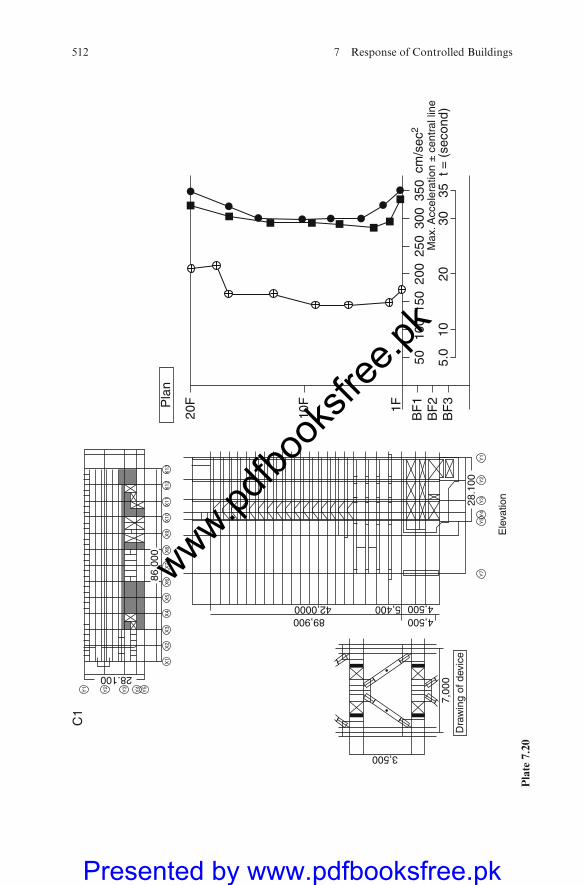
C1
5010
015
020
025
030
035
0cm
/sec
2
Max
. Acc
eler
atio
n ±
cen
tral
line
5.0
BF
3B
F2
BF
1
10F
20FPla
n
1F
1020
3035
t = (
seco
nd)
28.100
Y1
Y2
Y3
Y4
Y5
X1
X2
X3
X4
X5
X6
X7
X8
X9
X10
X11
X12
X13
86.0
00
28.1
00
4,5004,500
89,9005,40042,0000
Ele
vatio
n
Y1
Y2
Y3
Y4
Y5
Y7
7,00
0
3,500
Dra
win
g of
dev
ice
Plate
7.20
512 7 Response of Controlled Buildings
www.pdfbo
oksfr
ee.pk
Presented by www.pdfbooksfree.pk
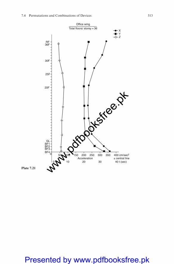
0 50 100 150 200 250Acceleration
300 350 400 cm/sec2
100 20 30
XYZ
BF4BF3
BF1BF2
GL
20F
25F
30F
36FRF
Office wing
Total floors/ storey = 36
± central line40 t (sec)
Plate 7.21
7.4 Permutations and Combinations of Devices 513
www.pdfbo
oksfr
ee.pk
Presented by www.pdfbooksfree.pk
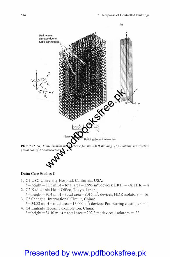
Data: Case Studies C
1. C1 USC University Hospital, California, USA:h=height=33.5 m; A=total area=3,995 m2; devices: LRH= 68; IHR= 8
2. C2 Kadokania Head Office, Tokyo, Japan:h=height=30.4 m; A=total area=8016 m2; devices: HDR isolators = 16
3. C3 Shanghai International Circuit, China:h=34.82 m; A=total area=13,000 m2; devices: Pot bearing elastomer = 4
4. C4 Linhailu Housing Completion, China:h=height=34.10 m; A=total area=202.3 m; devices: isolators = 22
Plate 7.22 (a) Finite element mesh scheme for the SMB Building. (b) Building substructure(total No. of 20 substructures)
514 7 Response of Controlled Buildings
www.pdfbo
oksfr
ee.pk
Presented by www.pdfbooksfree.pk
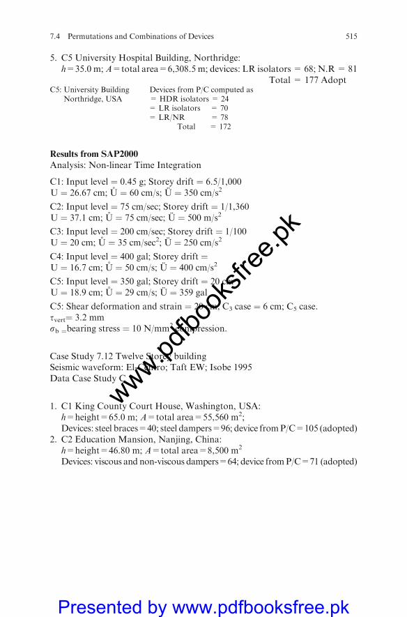
5. C5 University Hospital Building, Northridge:h=35.0 m;A=total area=6,308.5 m; devices: LR isolators = 68; N.R= 81
Total = 177 AdoptC5: University Building Devices from P/C computed as
Northridge, USA = HDR isolators = 24= LR isolators = 70= LR/NR = 78
Total = 172
Results from SAP2000
Analysis: Non-linear Time Integration
C1: Input level ¼ 0.45 g; Storey drift ¼ 6.5/1,000U ¼ 26.67 cm; U ¼ 60 cm/s; U ¼ 350 cm/s2
C2: Input level ¼ 75 cm/sec; Storey drift ¼ 1/1,360U ¼ 37.1 cm; U ¼ 75 cm/sec; U ¼ 500 m/s2
C3: Input level ¼ 200 cm/sec; Storey drift ¼ 1/100U ¼ 20 cm; U ¼ 35 cm/sec2; U ¼ 250 cm/s2
C4: Input level ¼ 400 gal; Storey drift ¼U ¼ 16.7 cm; U ¼ 50 cm/s; U ¼ 400 cm/s2
C5: Input level ¼ 350 gal; Storey drift ¼ 20 cmU ¼ 18.9 cm; U ¼ 29 cm/s; U ¼ 359 gal
C5: Shear deformation and strain ¼ 20 cm; C3 case ¼ 6 cm; C5 case.tvert¼ 3.2 mmsb ¼bearing stress ¼ 10 N/mm2 compression.
Case Study 7.12 Twelve Storey buildingSeismic waveform: El-Centro; Taft EW; Isobe 1995Data Case Study C
1. C1 King County Court House, Washington, USA:h=height=65.0 m; A=total area=55,560 m2;Devices: steel braces=40; steel dampers=96; device fromP/C=105 (adopted)
2. C2 Education Mansion, Nanjing, China:h=height=46.80 m; A=total area=8,500 m2
Devices: viscous and non-viscous dampers=64; device fromP/C=71 (adopted)
7.4 Permutations and Combinations of Devices 515
www.pdfbo
oksfr
ee.pk
Presented by www.pdfbooksfree.pk
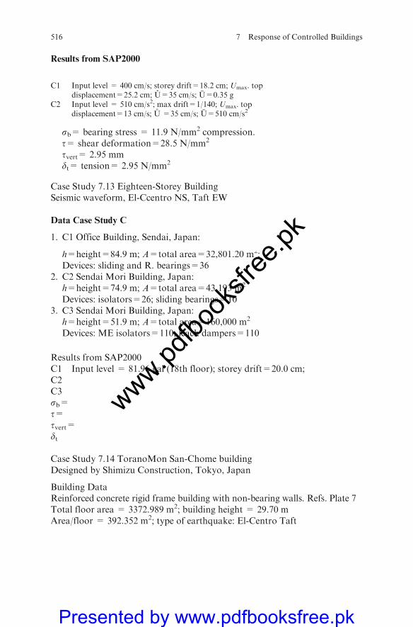
Results from SAP2000
C1 Input level = 400 cm/s; storey drift=18.2 cm; Umax. topdisplacement=25.2 cm; U=35 cm/s; U=0.35 g
C2 Input level = 510 cm/s2; max drift=1/140; Umax. topdisplacement=13 cm/s; U =35 cm/s; U=510 cm/s2
sb= bearing stress = 11.9 N/mm2 compression.t= shear deformation=28.5 N/mm2
tvert= 2.95 mmdt= tension= 2.95 N/mm2
Case Study 7.13 Eighteen-Storey BuildingSeismic waveform, El-Ccentro NS, Taft EW
Data Case Study C
1. C1 Office Building, Sendai, Japan:
h=height=84.9 m; A=total area=32,801.20 m2;Devices: sliding and R. bearings=36
2. C2 Sendai Mori Building, Japan:h=height=74.9 m; A=total area=43,193 m2
Devices: isolators=26; sliding bearings=103. C3 Sendai Mori Building, Japan:
h=height=51.9 m; A=total area=160,000 m2
Devices: ME isolators=110; leach dampers=110
Results from SAP2000C1 Input level = 81.96 gal (18th floor); storey drift=20.0 cm;C2C3sb=t=tvert=dt
Case Study 7.14 ToranoMon San-Chome buildingDesigned by Shimizu Construction, Tokyo, Japan
Building DataReinforced concrete rigid frame building with non-bearing walls. Refs. Plate 7Total floor area = 3372.989 m2; building height = 29.70 mArea/floor = 392.352 m2; type of earthquake: El-Centro Taft
516 7 Response of Controlled Buildings
www.pdfbo
oksfr
ee.pk
Presented by www.pdfbooksfree.pk
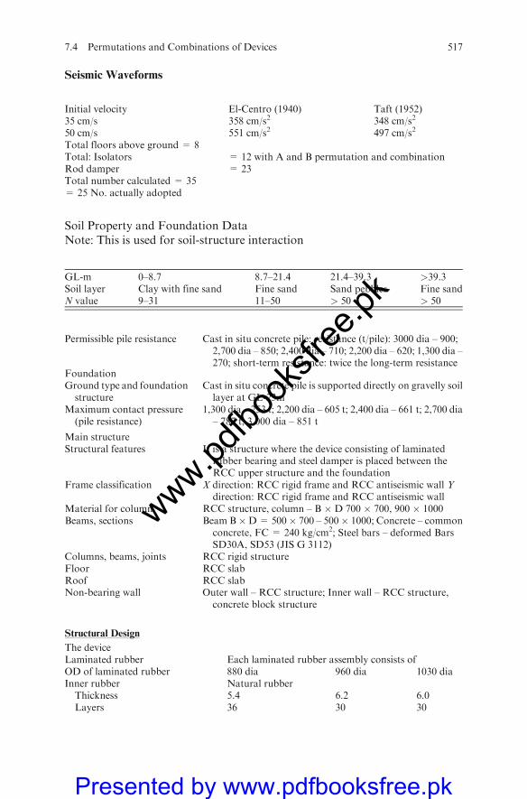
Seismic Waveforms
Initial velocity El-Centro (1940) Taft (1952)35 cm/s 358 cm/s2 348 cm/s2
50 cm/s 551 cm/s2 497 cm/s2
Total floors above ground = 8Total: Isolators = 12 with A and B permutation and combinationRod damper = 23Total number calculated = 35= 25 No. actually adopted
Soil Property and Foundation DataNote: This is used for soil-structure interaction
GL-m 0–8.7 8.7–21.4 21.4–39.3 >39.3Soil layer Clay with fine sand Fine sand Sand pebbles Fine sandN value 9–31 11–50 > 50 > 50
Permissible pile resistance Cast in situ concrete pile: resistance (t/pile): 3000 dia – 900;2,700 dia – 850; 2,400 dia – 710; 2,200 dia – 620; 1,300 dia –270; short-term resistance: twice the long-term resistance
FoundationGround type and foundationstructure
Cast in situ concrete pile is supported directly on gravelly soillayer at GL-23m
Maximum contact pressure(pile resistance)
1,300 dia – 253 t; 2,200 dia – 605 t; 2,400 dia – 661 t; 2,700 dia– 787 t; 3,000 dia – 851 t
Main structureStructural features It is a structure where the device consisting of laminated
rubber bearing and steel damper is placed between theRCC upper structure and the foundation
Frame classification X direction: RCC rigid frame and RCC antiseismic wall Ydirection: RCC rigid frame and RCC antiseismic wall
Material for column RCC structure, column – B � D 700 � 700, 900 � 1000Beams, sections Beam B�D= 500� 700 – 500� 1000; Concrete – common
concrete, FC = 240 kg/cm2; Steel bars – deformed BarsSD30A, SD53 (JIS G 3112)
Columns, beams, joints RCC rigid structureFloor RCC slabRoof RCC slabNon-bearing wall Outer wall – RCC structure; Inner wall – RCC structure,
concrete block structure
Structural Design
The deviceLaminated rubber Each laminated rubber assembly consists ofOD of laminated rubber 880 dia 960 dia 1030 diaInner rubber Natural rubberThickness 5.4 6.2 6.0Layers 36 30 30
7.4 Permutations and Combinations of Devices 517
www.pdfbo
oksfr
ee.pk
Presented by www.pdfbooksfree.pk
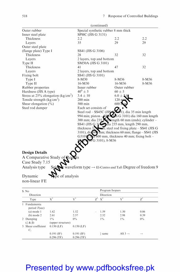
(continued)
Outer rubber Special synthetic rubber 8 mm thickInner steel plate SPHC (JIS G 3131)Thickness 2.2 2.2 2.2Layers 35 29 29
Outer steel plate(flange plate) Type I SS41 (JIS G 3106)Thickness 28 32 32Layers 2 layers, top and bottom
Type II SM50A (JIS G 3101)Thickness 41 47 32Layers 2 layers, top and bottom
Fixing bolt SS41 (JIS G 3101)Type I 8-M30 8-M36 8-M36Type II 16-M30 16-M36 8-M36
Rubber properties Inner rubber Outer rubberHardness (JIS A type) 400 � 5 60 � 5Stress at 25% elongation (kg/cm2) 3.4 � 10 6.0 � 2.0Tensile strength (kg/cm2) 200 min 120 minShear elongation (%) 500 min 600 minSteel rod damper Each set consists of
Steel rod – SS45C (JIS G 4501), dia 35 min length994 min; piston – SS41 (JIS G 3101) dia 160 mm length300 mm; dia 235 mm, length 60 mm (ends); cylinder –SS41 (JIS G 3101), dia 235 mm, length 290 mm,thickness 32.5 mm; steel rod fixing plate – SS41 (JIS G3101), dia 600 mm; thickness 60 mm; flange – SS41 (JISG3101), dia 600 mm, thickness 40 mm; fixing bolt –SS41 (JIS G 3101), 8-M36
Design Details
A Comparative Study of ResultsCase Study 7.15Analysis type Seismic waveform type! El-Centro and Taft Degree of freedom 9
Type of analysisDynamic
non-linear FE
S. No Program Isopars
Direction Direction
Type X* Y* Z* X* Y* Z*
1 Fundamenta
period T(sec)
(a) mode 1 1.62 1.52 – 1.59 1.50 0.06
(b) mode 2 2.61 2.57 2.52 2.98 0.39
2 Damping
(x & b)1%
(upper structure)
0% 1% 1% 0%
3 Shear coefficient
Ci
0.150 (LF) 0.150 (LF)
0.191 (IF) 0.191 (IF) } same AS 3! !0.296 (TF) 0.296 (TF)
518 7 Response of Controlled Buildings
www.pdfbo
oksfr
ee.pk
Presented by www.pdfbooksfree.pk
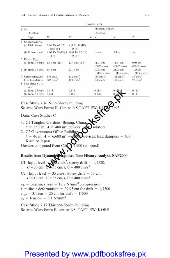
(continued)
S. No Program Isopars
Direction Direction
Type X* Y* Z* X* Y* Z*
4 Seismic load %
(a) Rigid frame 35 (LF); 62 (IF)
108 (TF)
4 (LF), 18 (IF)
45 (TF)
(b) Pressure wall 65 (LF); 38 (IF) 8
(TF)
96 (LF), 82 (IF)
55 (TF)
} same AS! !
5 Device Umax
(a) Input 35 cm/s 12.5 cm (Taft) 12.4 cm (Taft) 11.71 cm
(El-Centro)
11.67 cm
(El-Centro)
0.05 cm
(El-Centro)
6 (b) Input 50 cm/s 18.4 cm 23.10 cm 17.93 cm
(El-Centro)
21.75 cm
(El-Centro)
1.25 cm
(El-Centro)
7 Upper structure 146 cm/s2 132 cm/s2 138 cm/s2 128 cm/s2 50 cm/s2
U at foundation 203 cm/s2 189 cm/s2 198 cm/s2 190 cm/s2 75 cm/s2
8 Max shear Ci 1st
floor
(a) Input 35 cm/s 0.113 0.118 0.114 0.120 0.110
(b) Input 50 cm/s 0.164 0.186 0.170 0.190 0.113
Case Study 7.16 Nine-Storey buildingSeismic WaveForm: El-Centro NS TAFT EW, KUBA 1995
Data: Case Studies C
1. C1 Tonghui Gardens, Beijing, China:h = 33.2 m, A = 480 m2; devices: LRB isolators
2. C2 Government Office Building:h = 46 m, A = 6,680 m2 = 4,200; devices: lead dampers = 600Kushiro Japan
Devices computed from C/P = 4,900 (adopted)
Results from Dynamic Response, Time History Analysis SAP2000
C1: Input level = 400 cm/s2; storey drift = 1/7520;U=20 cm, U=35 cm/s, U=400 cm/s2
C2 : Input level = 35 cm/s, storey drift = 13 cm;U=13 cm, U=35 cm/s, U=400 cm/s2
sb = bearing stress = 12.2 N/mm2 compressiont = shear deformation = 29.95 cm for drift = 1/7500tvert= 3.1 cm = 20 cm for drift = 1/500st = tension = 3.1 N/mm2
Case Study 7.17 Thirteen-Storey buildingSeismic WaveForm El-centro NS, TAFT EW; KOBE
7.4 Permutations and Combinations of Devices 519
www.pdfbo
oksfr
ee.pk
Presented by www.pdfbooksfree.pk
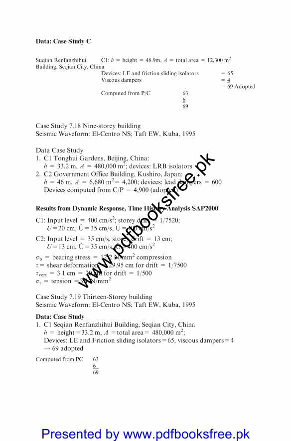
Data: Case Study C
Suqian Renfanzhihui C1: h = height = 48.9m, A = total area = 12,300 m2
Building, Seqian City, ChinaDevices: LE and friction sliding isolatorsViscous dampers
= 65= 4= 69 Adopted
Computed from P/C 63669
Case Study 7.18 Nine-storey buildingSeismic Waveform: El-Centro NS; Taft EW, Kuba, 1995
Data Case Study1. C1 Tonghui Gardens, Beijing, China:
h = 33.2 m, A = 480,000 m2; devices: LRB isolators2. C2 Government Office Building, Kushiro, Japan:
h = 46 m, A = 6,680 m2= 4,200; devices: lead dampers = 600Devices computed from C/P = 4,900 (adopted)
Results from Dynamic Response, Time History Analysis SAP2000
C1: Input level = 400 cm/s2; storey drift = 1/7520;U=20 cm, U=35 cm/s, U=400 cm/s2
C2: Input level = 35 cm/s, storey drift = 13 cm;U=13 cm, U=35 cm/s, U=400 cm/s2
sb = bearing stress = 12.2 N/mm2 compressiont= shear deformation = 29.95 cm for drift = 1/7500tvert = 3.1 cm = 20 cm for drift = 1/500st = tension =3.1 N/mm2
Case Study 7.19 Thirteen-Storey buildingSeismic Waveform: El-Centro NS; Taft EW, Kuba, 1995
Data: Case Study
1. C1 Seqian Renfanzhihui Building, Seqian City, Chinah = height=33.2 m, A =total area= 480,000 m2;Devices: LE and Friction sliding isolators=65, viscous dampers=4! 69 adopted
Computed from PC 63669
www.pdfbo
oksfr
ee.pk
Presented by www.pdfbooksfree.pk
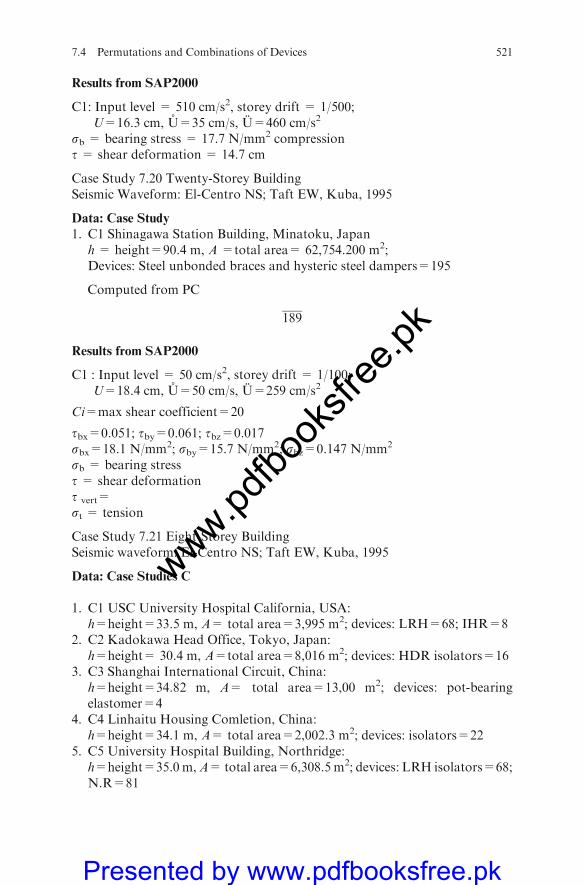
Results from SAP2000
C1: Input level = 510 cm/s2, storey drift = 1/500;U=16.3 cm, U=35 cm/s, U=460 cm/s2
sb = bearing stress = 17.7 N/mm2 compressiont = shear deformation = 14.7 cm
Case Study 7.20 Twenty-Storey BuildingSeismic Waveform: El-Centro NS; Taft EW, Kuba, 1995
Data: Case Study
1. C1 Shinagawa Station Building, Minatoku, Japanh = height=90.4 m, A =total area= 62,754.200 m2;Devices: Steel unbonded braces and hysteric steel dampers=195
Computed from PC
189
Results from SAP2000
C1 : Input level = 50 cm/s2, storey drift = 1/100;U=18.4 cm, U=50 cm/s, U=259 cm/s2
Ci=max shear coefficient=20
tbx=0.051; tby=0.061; tbz=0.017sbx=18.1 N/mm2; sby=15.7 N/mm2; sbz=0.147 N/mm2
sb = bearing stresst = shear deformationt vert=st = tension
Case Study 7.21 Eight-Storey BuildingSeismic waveform: El-Centro NS; Taft EW, Kuba, 1995
Data: Case Studies C
1. C1 USC University Hospital California, USA:h=height=33.5 m, A= total area=3,995 m2; devices: LRH=68; IHR=8
2. C2 Kadokawa Head Office, Tokyo, Japan:h=height= 30.4 m, A=total area=8,016 m2; devices: HDR isolators=16
3. C3 Shanghai International Circuit, China:h=height=34.82 m, A= total area=13,00 m2; devices: pot-bearingelastomer=4
4. C4 Linhaitu Housing Comletion, China:h=height=34.1 m, A= total area=2,002.3 m2; devices: isolators=22
5. C5 University Hospital Building, Northridge:h=height=35.0 m,A=total area=6,308.5 m2; devices: LRH isolators=68;N.R=81
7.4 Permutations and Combinations of Devices 521
www.pdfbo
oksfr
ee.pk
Presented by www.pdfbooksfree.pk
Devices computed from P/C:
=HDR isolators = 24= LR isolators = 70=LR/NR = 78
172
Results from SAP2000
Analysis Non-linear Time Integration
C1: Input level = 0.45 g; storey drift = 6.5/1,000;U=25.67 cm, U=60 cm/s, U=350 cm/s2
C2: Input level = 75 cm/s, storey drift = 1/1360;U=37.1 cm, U=75 cm/s, U=500 cm/s2
C3: Input level = 200 cm/cm2; storey drift = 1/1000;U=20.0 cm, U=35.0 cm/s, U=250 cm/s2
C4: Input level = 400 gal, storey drift =20 cmU=16.7 cm, U=50 cm/s, U=400 cm/s2
C5: Input level = 350 gal, storey drift =U=18.7 cm, U=29 cm/s, U=3,590 cm/s2
sb = bearing stress = 10.0 N/mm2 compressiont = shear deformation and strain= 20.0 cm for C3 case
= 6.0 cm for C5 casetvert= 3.2 mmst = tension =3.1 N/mm2
Case Study 7.22 Eight Story BuildingSeismic Waveform: El-Centro NS; Taft EW, Kuba, 1995
Data: Case Studies C
1. C1 Los Angeles City Hall, LA, USA:h=height=42.0 m, A= total area=100,406.7 m2;Devices: Isolators (HDR+SLB=viscous dampers)=526 actually placedIsolators (HDR+SLB=viscous dampers)= *59 (calculated)
C1: Input level = MCE (10% in 100 years); storey drift=3/1000;U=53.30 cm, U=35 cm/s, U=0.35 g
Results from SAP2000 and Program ISOPAR for checking results*using permutation/combination and finally checked by time history
analysis
tbx=0.071; tby=0.019; tbz=0.020sbx=20.2 N/mm2; sby=17.7 N/mm2; sbz=0.158 N/mm2
Ci=0.31
Total floors/storeys= 36
522 7 Response of Controlled Buildings
www.pdfbo
oksfr
ee.pk
Presented by www.pdfbooksfree.pk
7.5 Seismic Design of Tall Buildings in Japan – A Comprehensive
Study
7.5.1 General Introduction
Kiyushi Muto in his report (MUTO Report 73-1-1, May 1973) laid out a
comprehensive method for the planning and design of tall buildings (h�45mand h>45m) in Japan. In order to obtain horizontal seismic coefficients,
Tables 10.14 and 10.15 give preliminary calculations based on an old Japanese
code. In the same section, the work has been modified by including the effects
of vertical acceleration. The SMB building of 55 storeys is taken as a study
case (Plate 7.8).The Muto Institute has provided a flow chart (Fig. 7.1) which indicates the
AIJ guidelines for the seismic analysis and design of tall buildings in Japan. It is
suggested that preliminary design planning be checked and analysed against
several earthquakes. Dynamic analysis is performed using a rigorous vibration
model in conjunction with structural stiffness. A series of computer programs
have been developed (FAPP I to FAPP IV) for steel structures. Figures 7.9 and
gives a brief illustration of what these computer programs can do. Examples in
Table 3.18 indicate the response control in actual tall buildings.After developing a sound technique for planning, testing various buildings and
obtaining a criterion for the seismic analysis of tall buildings, the Muto Institute
took up the case of the Shinjuku Mitsui Building (SMB) in Tokyo, a 55-storey,
225m high office building as shown in Plate 7.8. Typical floor areas are
58.4�44.5m. The building has sufficient stiffness against strong winds and
typhoons, which frequently occur in Japan. The stiffness of this building was
assessed initially by a value given by the fundamental natural period T1 =0.1N
where N is the number of storeys. Hence T1 =0.1 � 55=5.5 seconds. Various
layouts and schemes were considered but T1 was not sufficient in the transverse
direction. The final suitable design layout is shown in the Muto Report.The El-Centro Earthquake was considered as the basis for the animated
earthquake response of the SMB building.
7.5.2 Resimulation Analysis of SMB Based on the KobeEarthquake Using Three-Dimensional Finite ElementAnalysis
The earthquake of 17 January 1995 that occurred in the area of Kobe in
southwestern Japan, also known as the Hanshin or Hyogo-Ken Nanbu Earth-
quake, caused extensive damage and numerous casualties. The magnitude of
this earthquake was M=7.2. Various universities and institutes in Japan
reported crust deformations, the foreshocks, with around 6,000 events
7.5 Seismic Design of Tall Buildings in Japan – A Comprehensive Study 523
www.pdfbo
oksfr
ee.pk
Presented by www.pdfbooksfree.pk
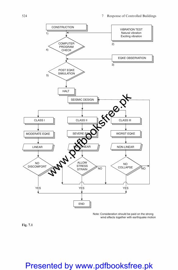
VIBRATION TESTNatural vibrationExciting vibration
EQKE OBSERVATION
POST EQKESIMULATION
HALT
CLASS I CLASS II CLASS III
SEISMIC DESIGN
COMPUTERPROGRAM
CHECK
MODERATE EQKE
LINEAR
NODISCOMFORT
ALLOWSTRESSSTRAIN
NOCOLLAPSENONO NO
END
NON-LINEAR NON-LINEAR
SEVERE EQKE WORST EQKE
Note: Consideration should be paid on the strong wind effects together with earthquake motion
1)
4)
5)
2)
3)
YES YESYES
CONSTRUCTION
Fig. 7.1
524 7 Response of Controlled Buildings
www.pdfbo
oksfr
ee.pk
Presented by www.pdfbooksfree.pk
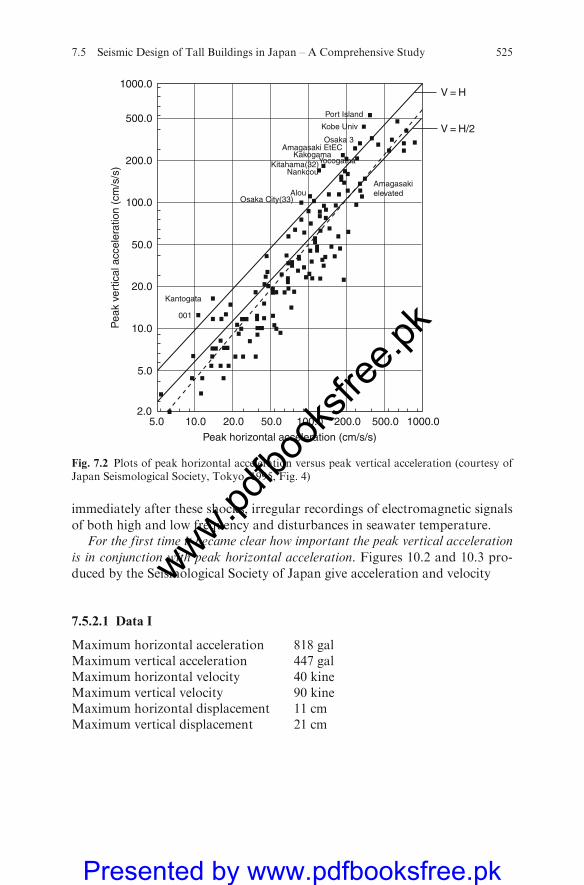
immediately after these shocks, irregular recordings of electromagnetic signals
of both high and low frequency and disturbances in seawater temperature.For the first time it became clear how important the peak vertical acceleration
is in conjunction with peak horizontal acceleration. Figures 10.2 and 10.3 pro-
duced by the Seismological Society of Japan give acceleration and velocity
7.5.2.1 Data I
Maximum horizontal acceleration 818 galMaximum vertical acceleration 447 galMaximum horizontal velocity 40 kineMaximum vertical velocity 90 kineMaximum horizontal displacement 11 cmMaximum vertical displacement 21 cm
1000.0
500.0
200.0
100.0
50.0
20.0
10.0
5.0
2.05.0 10.0 20.0 50.0 100.0 200.0 500.0 1000.0
Peak horizontal acceleration (cm/s/s)
Pea
k ve
rtic
al a
ccel
erat
ion
(cm
/s/s
)
V = H
V = H/2
Amagasakielevated
Port Island
Kobe Univ
Osaka 3Amagasaki EtEC
KakogamaYocogamaKitahama(32)
Nankcou
Osaka City(33)
001
Kantogata
Alou
Fig. 7.2 Plots of peak horizontal acceleration versus peak vertical acceleration (courtesy ofJapan Seismological Society, Tokyo, 1995, Fig. 4)
7.5 Seismic Design of Tall Buildings in Japan – A Comprehensive Study 525
www.pdfbo
oksfr
ee.pk
Presented by www.pdfbooksfree.pk
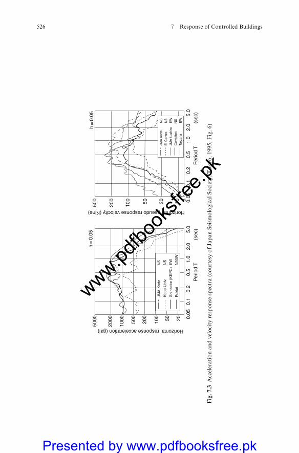
5000
h =
0.0
5h
= 0
.05
2000
1000 500
200
100 50 20 0.
055102050100
200
500
0.1
0.2
0.5
1.0
2.0
5.0
Horizontal response acceleration (gal)
Horizontal pseudo response velocity (Kine)
0.05
0.1
0.2
0.5
1.0
2.0
5.0
Per
iod
T(s
ec)
Per
iod
T(s
ec)
JMA
Kod
eN
S
Kob
e U
niv.
Shi
nkob
e (K
EP
C)
Fuk
iai
NS
EW
N30
W
JMA
Kod
eN
S
Cor
ralit
os
Tarz
ana
NS
NS
EW
EW
El C
entr
o
JMA
kus
hiro
Fig.7.3
Accelerationandvelocity
response
spectra(courtesyofJapanSeism
ologicalSociety,Tokyo,1995,Fig.6)
526 7 Response of Controlled Buildings
www.pdfbo
oksfr
ee.pk
Presented by www.pdfbooksfree.pk
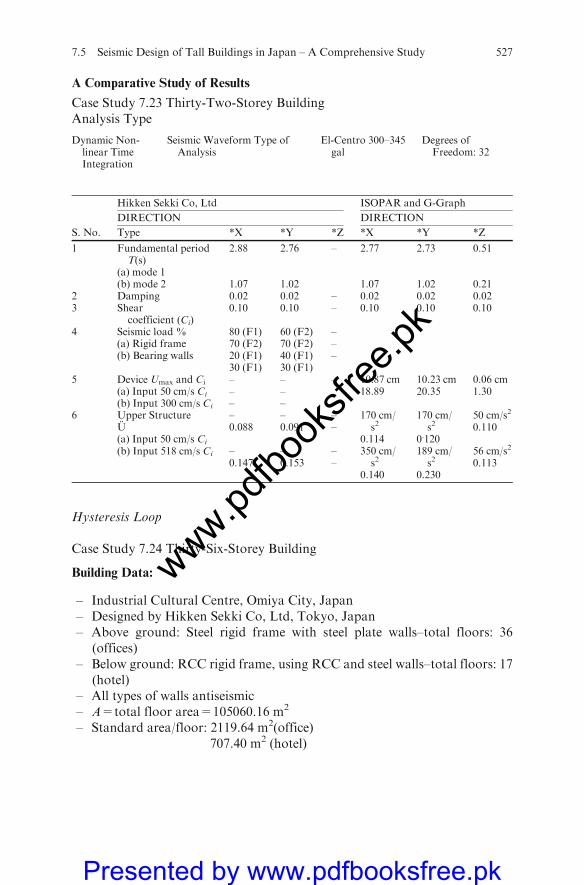
A Comparative Study of Results
Case Study 7.23 Thirty-Two-Storey BuildingAnalysis Type
Dynamic Non-linear TimeIntegration
Seismic Waveform Type ofAnalysis
El-Centro 300–345gal
Degrees ofFreedom: 32
Hikken Sekki Co, Ltd ISOPAR and G-Graph
DIRECTION DIRECTION
S. No. Type *X *Y *Z *X *Y *Z
1 Fundamental periodT(s)
2.88 2.76 – 2.77 2.73 0.51
(a) mode 1(b) mode 2 1.07 1.02 1.07 1.02 0.21
2 Damping 0.02 0.02 – 0.02 0.02 0.023 Shear
coefficient (Ci)0.10 0.10 – 0.10 0.10 0.10
4 Seismic load % 80 (F1) 60 (F2) –(a) Rigid frame 70 (F2) 70 (F2) –(b) Bearing walls 20 (F1)
30 (F1)40 (F1)30 (F1)
–
5 Device Umax and Ci – – – 10.87 cm 10.23 cm 0.06 cm(a) Input 50 cm/s Ci – – 18.89 20.35 1.30(b) Input 300 cm/s Ci – –
6 Upper StructureU(a) Input 50 cm/s Ci
–0.088
–0.091
––
170 cm/s2
0.114
170 cm/s2
0.120
50 cm/s2
0.110
(b) Input 518 cm/s Ci –0.147
–0.153
––
350 cm/s2
0.140
189 cm/s2
0.230
56 cm/s2
0.113
Hysteresis Loop
Case Study 7.24 Thirty-Six-Storey Building
Building Data:
– Industrial Cultural Centre, Omiya City, Japan– Designed by Hikken Sekki Co, Ltd, Tokyo, Japan– Above ground: Steel rigid frame with steel plate walls–total floors: 36
(offices)– Below ground: RCC rigid frame, using RCC and steel walls–total floors: 17
(hotel)– All types of walls antiseismic– A=total floor area=105060.16 m2
– Standard area/floor: 2119.64 m2(office)707.40 m2 (hotel)
7.5 Seismic Design of Tall Buildings in Japan – A Comprehensive Study 527
www.pdfbo
oksfr
ee.pk
Presented by www.pdfbooksfree.pk

(continued)
–Total number ofisolators: 12
Total number of isolators and dampers evaluatedfrom P/C-evaluated Non-linear Time Analysis = 21
–Dampers: 618
H=building height Office wing 136.550 mHotel wing 57.050 m
H=max height of the structure Office wing 140.050 mHotel wing 57.050 m
Standard floor height Office wing 3.8 mHotel wing 3.2 m
Height of first floor Office wing 5,500 mHotel wing –
Height of the equipment floor Office wing (13th floor) 5,500 mHotel wing –
Height of basement floor Office wing 5,800 mHotel wing (B1 floor) 5,800
Floors
Above ground Office wing 31Hotel wing 13
Below ground Office wing 4Hotel wing 3
Penthouse Office wing 1Hotel wing 1
Soil Property and Foundation Data
Note (used also for soil–structure interaction)
Soil Property and N value
GL-m Soil layerNvalue
0.0–5.0 Loam and clay (lm. DT) 1–55.0–10.0 Sandy soil, cohesive soil (Dc2, Dc1) 3–3410.0–26.0 Sandy soil � (D2) 16–4426.0–41.0 Cohesive soil (Dc2, Dc3) 4–4441.0–43.0 Alternate layers of gravel, sandy soil and cohesive
soil14–50
43.0–48.0 Cohesive soil � (Dc4) 10–1548–63 Sandy soil � (D3) 30–50
Permissiblegroundresistance
Pile resistance: 250t/m2
528 7 Response of Controlled Buildings
www.pdfbo
oksfr
ee.pk
Presented by www.pdfbooksfree.pk

Ground Property
Foundation depth Office wing 25.250 mHotel wing 17.450 m
Ground type, foundation structure Pile foundationMaximum contact pressure (Pile resistance) 210 t/m2(pile)
Main Structure
Structural features In both X and Y directions, rigid frames containing antiseismicsteel plate walls at the core are provided
Frame classification Structure above ground: RCC rigid frames using steel plate walls;Structure below ground: RCC rigid frame using RCC antiseismic
walls and steel framesBearing walls, other walls Structure above ground: Steel plate antiseismic walls
Structure below ground: RCC antiseismic wallsMaterial for columns,beams, sections
Structure above ground: Column – 600�600 with a box-like cross-section;
Beam-welded I section with depths of 850, 1200, 1500Structure below ground: Column – 1100�1100 and 1000�1000;
Beam – 850�1200 and 850�900Steel frame – SM50; Steel bars – SD35, SD30;Concrete – Floor above ground: light concrete strength – 180 kg/cm2
(sp. gr. 1.75, 1.85);Floor below first floor: common concrete strength – 210 kg/cm2
Columns, beams, joints Structure above ground: Beam flange welded at site. Beam webfixed with HT bolts and columns welded at site;
Structure below ground: Steel sections fixed with HT bolts(columns and beams, factory welded)
Floor Structure above ground: RCC slabStructure below ground: RCC slab
Roof Cast in situ concrete structureNon-bearing walls Outer wall – Precast concrete structure;
Inner wall – Light steel frame with laminated PB
7.5.3 Data I
Maximum horizontal acceleration = 818 galMaximum vertical acceleration = 447 galMaximum vertical velocity = 40 kineMaximum horizontal velocity = 90 kine
7.5 Seismic Design of Tall Buildings in Japan – A Comprehensive Study 529
www.pdfbo
oksfr
ee.pk
Presented by www.pdfbooksfree.pk
7.5.4 Data II
In the finite element analysis dynamic equations given in the Appendix, the
damping ratio is 10%. Isoparametric four-noded solid elements are used for the
finite element discretization. The following gives additional data:
1. SBM 55-storey frame and floorsFloor: Four-noded solid elements (55,500)Frame: Four-noded line elements (220,000)
2. Soil–structure interaction2,400 nodes on ground surface2,200 nodes on ground–structure interface
Reference is made to the soil–structure analysis in Chap. 6.
7.5.4.1 Provision of Controlled Devices
(a) Total number of isolators=1,650 computed with P/C and non-linear timeintegrationTotal number of HAD type=1,620 provided by designers (HRD)Total number of dampers:
(b) Viscoelastic computed=335Viscoelastic provided =365*
(c) Viscous computed=155 with P/C calculation and non-linear timeintegrationViscous provided =159* by the designers
(d) Sensors=80
*Note: Positions available in the building where the devices could easily be
accommodated.
Results based on ISOPAR-II
Ground period Tc=0.6 secPrimary design period T Tx1=2.88; Ty1=2.76; Tz1=1.35Design shear coefficient Ci Along the length: 0.10; along the width: 010;
distribution pattern: it includes the sheardistribution as obtained from the vibrationresponse analysis
Horizontal seismic intensityat the foundation K
The seismic intensity K at 1F: 0.10; the seismicat GL-40m=0. In between, it is interpolatedassuming a straight line relationship
Maximum storey drift 3/1000Maximum horizontal and vertical displacements respectively 11cm and 21cm
� Computer CRAY-3
530 7 Response of Controlled Buildings
www.pdfbo
oksfr
ee.pk
Presented by www.pdfbooksfree.pk
tbx=0.10; tby=0.10; tbz=0.022sbx=25.3 N/mm2; sby=19.3 N/mm2; sbz=0.23 N/mm2
Acceleration time relation is drawn in 10.16, giving values in three directionsX,Y and Z.
7.5.4.2 Finite Element Analysis: Non-linear Time Integration
Programs ISOPAR and SAP2000 have been used to check each other’s vali-dated results and to check certain specialized data and results.
The finite element mesh scheme with boundary conditions defined is shownin Plate 7.23. The step-by-step time integration analysis is adopted as part ofthis dynamic finite element analysis. The loadings given by theMuto Institute inFig. . ...are adopted as the input data to the three-dimensional finite elementanalysis.
For reasons of economics in the overall performance of time-consumingsolution procedures, the entire structure is divided into seven No. 8 substruc-tures. The loading on one substructure from the Muto seismic analysis is givenin Fig. 7.4. All columns are 500�500 mm box-type fully welded and rigidlyconnected to a girder. The transverse framing consists of wall frames, openframes and braced frames.Deadweight is assumed to be 115 kg/m2(1.045KN/m2).A non-linear earthquake of 0.5 g was assumed for this study.
Due to the inclusion of vertical acceleration simultaneously with the hor-izontal acceleration, the approach is completely changed. If this building werelocated in the Kobe region during the earthquake, the damage to the floors andframes would be in the ratio of three times the damage if vertical accelerationwere not ignored. The deformation shear and overturning moments by theProgram ETABS, checked by Programs ISOPAR and SAP2000 for the ani-mated earthquake responses, would be on average four times more. A compara-tive study of the displacement–time function graph (Fig. 10.5) indicated amarked difference for the Kobe earthquake. All seismic devices were placedand functionable.
The SM building is taken as an example for the three-dimensional dynamicfinite element analysis in which material and geometric non-linearity are con-sidered. Figure 10.16 shows ductility models for the various materials adopted.These models are included in the program ISOPAR (extended three-dimen-sional analysis of building systems) developed byWilson et al. at the Universityof California. The building is idealized as independent frames and sub-framesinterconnected by a flooring system adopted by the Muto Institute. Axial,bending and shear deformations are included within each column made of500�500 welded box-type members. Beams, girders and vertical panel elementsallow discontinuity. The loadings evaluated accurately by the Muto Institutefor the SBM building have been modified to include the effects of both hor-izontal and vertical acceleration. Non-linear earthquakes of 0.5 g are consid-ered for Kobe and other earthquake locations, assuming the SMB is sited inthese areas as well.
7.5 Seismic Design of Tall Buildings in Japan – A Comprehensive Study 531
www.pdfbo
oksfr
ee.pk
Presented by www.pdfbooksfree.pk
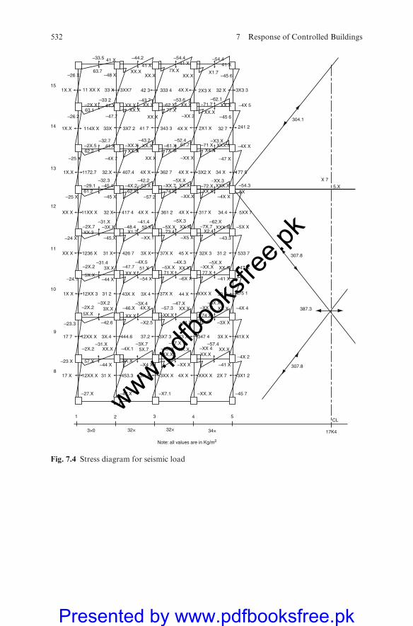
54321
3×0 32× 32× 34×
Note: all values are in Kg/m2
304.1
307.8
387.3
307.8
X 7
5.X
CL
17K4
–33.5 41 X
63.7–48 X
–33 2
3XX7 42 3 333 4
–47.7
–43.7
–44.2 –54.4 –54.4
4X.X 2X3 X
–4X 5
–45 6
–45 6
–71.7–62.1
32 X
41 X41 X41 X
3X3 3
–62.X77.X
–53.6
33 X
–2X.X
1X.X
–2X.5
–25 X –4X 7
1X.X 1172.7 32.X 407.4 4X X 4X X 3X2 X 177 5
–54.3
–4X X
–XX.3XXX.X
XX.X–XX.X
XXX.4–7X.7X2.4
–43.3–X5 X
–5X.XX1.7
52.X–48.4–41.4–31.X
–3X.X–2X.7XX.3
–45.X–24 X
XX X 31 X 3X X 45 X 32X 3 31.2
–47 X–5X.X
XX.X–XX.X77.X
–41 X–6X X–54 X–44 X
12XX 3 31 2 43X X 3X 4 44 X 30 X
–3X X
–5X.X
74 X
3X X 41X X
XXX X3XX X12XX X
12XX X
5X.X–2X.2
–3X.2
–31.4
3X.X
5X.X
–2X.2 3X.X
–23.3
453.3 4X X3X X31 X
3X.4
–44 X57.X
–2X.2–31.X
37.2 3X7 3
–27.X –47.X –X7.1
–XX X
43 X 347 4
–X4 X
17 X
17 7
–23 X
–XX. X
–4X 2
–41 X
–XX 4–XX.X
XX.X
XX.X
–XX.X
71.X
–46.X
–47.7
4X.X
51.X
–XX.X XX.XXX.X
XX.X
XX.X –4X.1–3X.7 –47.X
–61.X
–47.X
–4X.3–4X.5
–3X.4–57.3
–5X.X
–X2.5–42.6
5X.7XX.XXX.X
5X.X
444.6
XX.XXX.X–57.4
3X1 22X 7
–45 7
XXX X 475 1
–4X 4
37X X
–24.1
1X X
533 737X X1236 X 426 7
–5X.3
73.4XX.X
–XX.1
–5X.XXX.X–XX.7
–74.X–57 2
–53 X–42.2
–4X.262.X
–45 X
–45.4–32.3
–29.1
–25 X
XX X 11XX X 32 X 417 4 4X X 4X X361 2 317 X 5XX 7
–5X X
34.4
–62.X
12
11
10
9
8
13
61.2–72.X
5X
34 X
XX X
362 7
–32.741.X –XX.X
–43.2 –52.4–61.X 67.77X.4XX.X
XX.X62.2
114X X 33X 3X7 2 41 7 343 3
–26 263 1
41.X XX.X
XX.XXX.X XX.X
7X.X X1.7
XX.X
–XX X
XXX.5–X3.X
XX.XXX.X XX.X
XX.X
XX.X
2X1 X 32 7 241 24X X
–XX 2
–4X X
–47 X
–71 XX4.X
11 XX X1X.X
–26 X
15
14
Fig. 7.4 Stress diagram for seismic load
532 7 Response of Controlled Buildings
www.pdfbo
oksfr
ee.pk
Presented by www.pdfbooksfree.pk
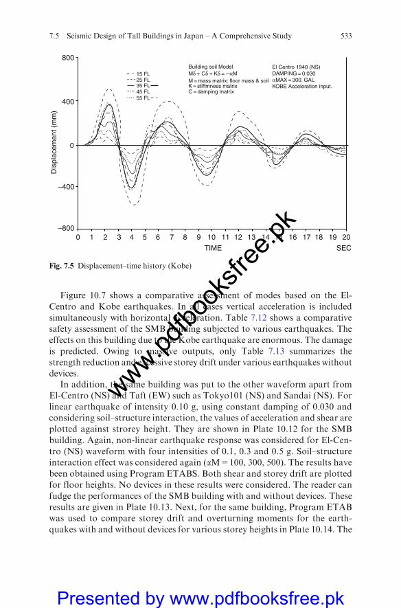
Figure 10.7 shows a comparative assessment of modes based on the El-
Centro and Kobe earthquakes. In all cases vertical acceleration is included
simultaneously with horizontal acceleration. Table 7.12 shows a comparative
safety assessment of the SMB building subjected to various earthquakes. The
effects on this building due to the Kobe earthquake are enormous. The damage
is predicted. Owing to massive outputs, only Table 7.13 summarizes the
strength reduction and excessive storey drift under various earthquakes without
devices.In addition, the same building was put to the other waveform apart from
El-Centro (NS) and Taft (EW) such as Tokyo101 (NS) and Sandai (NS). For
linear earthquake of intensity 0.10 g, using constant damping of 0.030 and
considering soil–structure interaction, the values of acceleration and shear are
plotted against strorey height. They are shown in Plate 10.12 for the SMB
building. Again, non-linear earthquake response was considered for El-Cen-
tro (NS) waveform with four intensities of 0.1, 0.3 and 0.5 g. Soil–structure
interaction effect was considered again (aM=100, 300, 500). The results have
been obtained using Program ETABS. Both shear and storey drift are plotted
for floor heights. No devices in these results were considered. The reader can
fudge the performances of the SMB building with and without devices. These
results are given in Plate 10.13. Next, for the same building, Program ETAB
was used to compare storey drift and overturning moments for the earth-
quakes with and without devices for various storey heights in Plate 10.14. The
0 1 2 3 4 5 6 7 8 9 10 11 12 13 14 15 16 17 18 19 20
800
–800
–400
0
400
Dis
plac
emen
t (m
m)
Building soil ModelMδ + Cδ + Kδ = – αM M = mass matrix: floor mass & soilK = stiffmness matrixC = damping matrix
15 FL25 FL35 FL45 FL55 FL
El Centro 1940 (NS)DAMPING = 0.030αMAX = 300. GALKOBE Acceleration input.
TIME SEC
Fig. 7.5 Displacement–time history (Kobe)
7.5 Seismic Design of Tall Buildings in Japan – A Comprehensive Study 533
www.pdfbo
oksfr
ee.pk
Presented by www.pdfbooksfree.pk
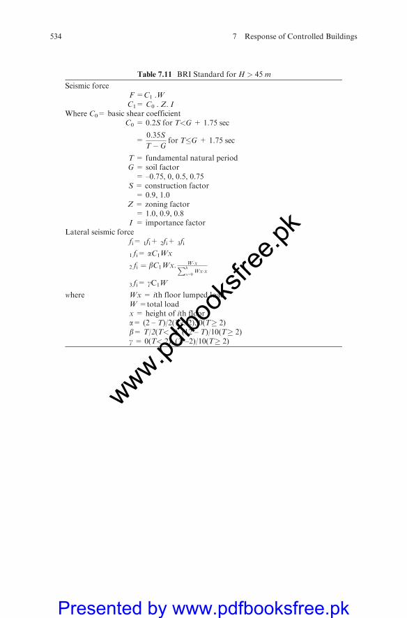
Table 7.11 BRI Standard for H > 45 m
Seismic forceF =C1 .WC1= C0 . Z. I
Where C0= basic shear coefficientC0 = 0.2S for T<G + 1.75 sec
=0:35S
T� Gfor T�G + 1.75 sec
T = fundamental natural periodG = soil factor= –0.75, 0, 0.5, 0.75
S = construction factor= 0.9, 1.0
Z = zoning factor= 1.0, 0.9, 0.8
I = importance factorLateral seismic force
fi= 1fi+ 2fi+ 3fi
1 fi= aC1Wx
2 fi ¼ bC1Wx: WxPh
x¼0 Wxx
3 fi= gC1W
where Wx = ith floor lumped loadW =total loadx = height of ith floora= (2 – T)/2(T< 2), 0(T 2)b= T/2(T< 2), (12 – T)/10(T 2)g = 0(T< 2), (T –2)/10(T 2)
534 7 Response of Controlled Buildings
www.pdfbo
oksfr
ee.pk
Presented by www.pdfbooksfree.pk
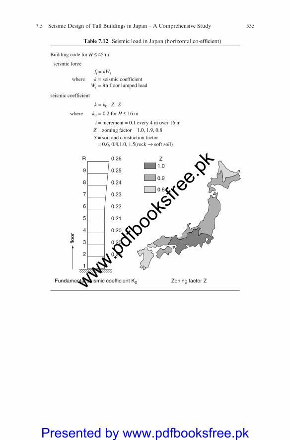
Table 7.12 Seismic load in Japan (horizontal co-efficient)
Building code for H ≤ 45 m
fi = kWi
k = k0 . Z . S
i = increment = 0.1 every 4 m over 16 m
Z = zoming factor = 1.0, 1.9, 0.8
S = soil and constuction factor = 0.6, 0.8,1.0, 1.5(rock → soft soil)
where k = seismic coefficient
where k0 = 0.2 for H ≤ 16 m
Wi = ith floor lumped load
seismic force
seismic coefficient
1
2
3
4
5 0.21
0.22
0.23
0.24
0.25
0.261.0Z
0.9
0.8
0.20
Zoning factor ZFundamental seismic coefficient K0
floor
0.20
0.20
6
7
8
9
R
7.5 Seismic Design of Tall Buildings in Japan – A Comprehensive Study 535
www.pdfbo
oksfr
ee.pk
Presented by www.pdfbooksfree.pk
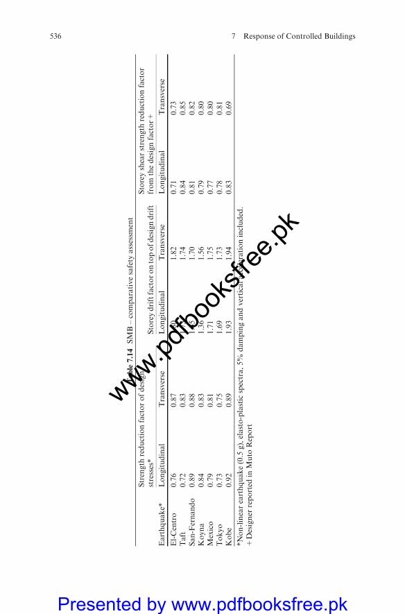
Table7.14
SMB–comparativesafety
assessm
ent
Earthquake*
Strength
reductionfactorofdesign
stresses*
Storeydriftfactorontopofdesigndrift
Storeyshearstrength
reductionfactor
from
thedesignfactor+
Longitudinal
Transverse
Longitudinal
Transverse
Longitudinal
Transverse
El-Centro
0.76
0.87
1.80
1.82
0.71
0.73
Taft
0.72
0.83
1.73
1.74
0.84
0.85
San-Fernando
0.89
0.88
1.65
1.70
0.81
0.82
Koyna
0.84
0.83
1.36
1.56
0.79
0.80
Mexico
0.79
0.81
1.71
1.75
0.77
0.80
Tokyo
0.73
0.75
1.69
1.73
0.78
0.81
Kobe
0.92
0.89
1.93
1.94
0.83
0.69
*Non-linearearthquake(0.5
g),elasto-plasticspectra,5%
dampingandverticalaccelerationincluded.
+Designer
reported
inMuto
Report
536 7 Response of Controlled Buildings
www.pdfbo
oksfr
ee.pk
Presented by www.pdfbooksfree.pk
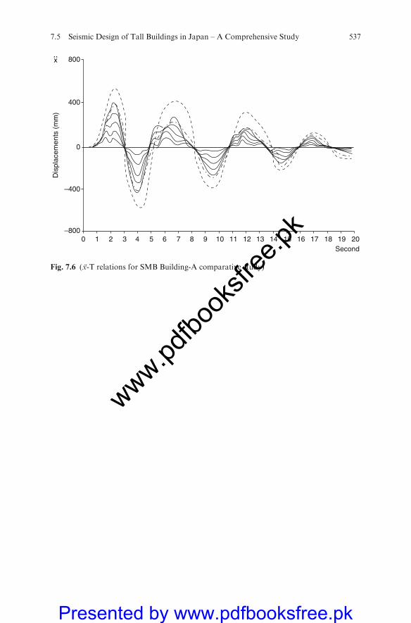
0 1 2 3 4 5 6 7 8 9 10 11 12 13 14 15 16 17 18 19 20Second
x• •
Dis
plac
emen
ts (
mm
)800
–800
–400
0
400
Fig. 7.6 (x-T relations for SMB Building-A comparative study)
7.5 Seismic Design of Tall Buildings in Japan – A Comprehensive Study 537
www.pdfbo
oksfr
ee.pk
Presented by www.pdfbooksfree.pk
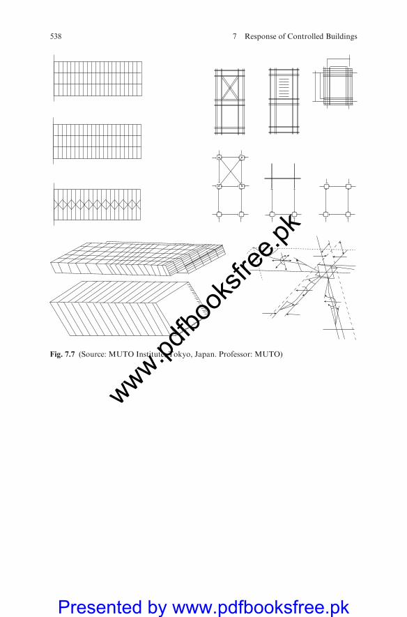
Fig. 7.7 (Source: MUTO Institute, Tokyo, Japan. Professor: MUTO)
538 7 Response of Controlled Buildings
www.pdfbo
oksfr
ee.pk
Presented by www.pdfbooksfree.pk
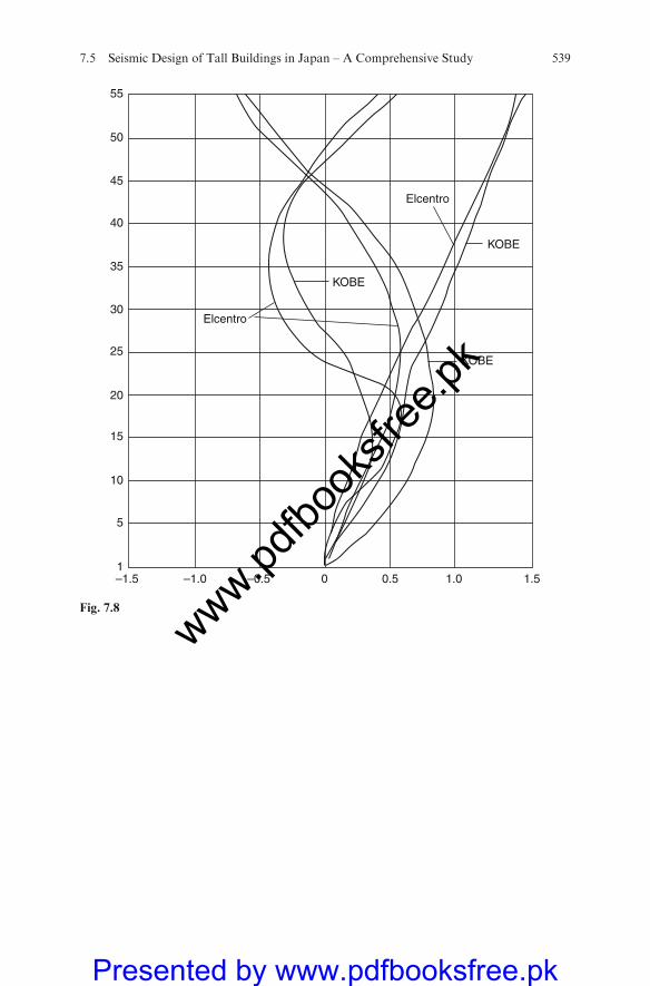
–1.0 –0.5 0 0.5 1.0 1.5–1.51
5
10
15
20
25
30
35
40
45
50
55
Elcentro
KOBE
KOBE
KOBE
Elcentro
Fig. 7.8
7.5 Seismic Design of Tall Buildings in Japan – A Comprehensive Study 539
www.pdfbo
oksfr
ee.pk
Presented by www.pdfbooksfree.pk

2,81
5
1,64
06,
500
280
S 630
100 1004040 6
6 125
505
2040
40
300
Section of view ofdevice
6,080 4,280
16,360
3 2 1
Section B-B
Section A-A
A B
3,26
43,
000
1,64
06,
500
280
3,26
43,
000
5,65
0
2,81
5
A
A A
B. FL
B. FL
B. FL
B
B
B
3 2
6,086 4,280
Plan
1
2,81
55,65
0
2,81
5
A
B
2,81
55,65
0 2,81
5
A
B
Fig. 7.9 (Source: MUTO Institute, Tokyo, Japan. Professor: MUTO)
Supersonicanchor
Elastomicbearing
(a) (b)
Fig. 7.10 (Source: MUTO Institute, Tokyo, Japan. Professor: MUTO)
540 7 Response of Controlled Buildings
www.pdfbo
oksfr
ee.pk
Presented by www.pdfbooksfree.pk
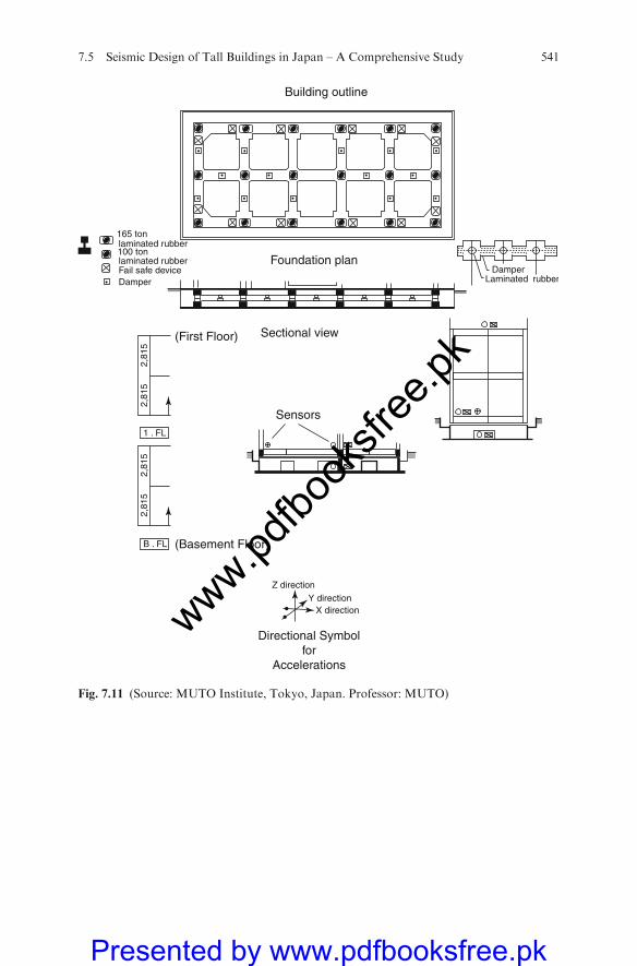
Building outline
DamperLaminated rubber
Foundation plan
Sectional view
165 ton
100 tonlaminated rubber
laminated rubberFail safe deviceDamper
Sensors1 . FL
(First Floor)
(Basement Floor)
Z directionY direction
X direction
B . FL
2,81
52,
815
2,81
52,
815
Directional Symbolfor
Accelerations
Fig. 7.11 (Source: MUTO Institute, Tokyo, Japan. Professor: MUTO)
7.5 Seismic Design of Tall Buildings in Japan – A Comprehensive Study 541
www.pdfbo
oksfr
ee.pk
Presented by www.pdfbooksfree.pk
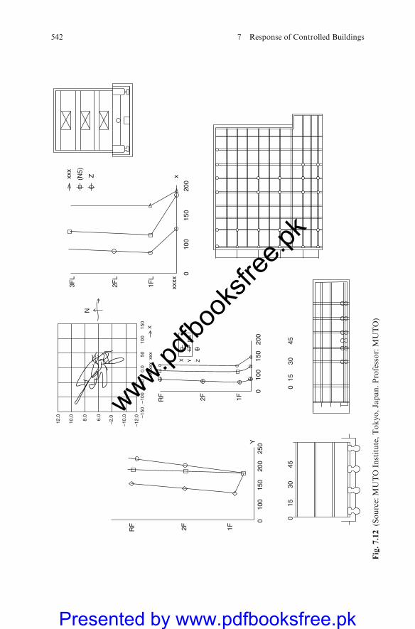
3FL
N
12.0
10.0
8.0
6.0
–2.0
–12.
0 –150
–100
–50
0.0
50
xxxx
xx x
xx
X YN
S
Z
X
100
150
–10.
0
2FL
RF 2F 1F
010
015
020
025
00
100
015
3045
015
3045
150
200
Y
Z(N5)
xxx
1FL
1F2FRF
xxxx
010
015
020
0
x
Fig.7.12(Source:MUTO
Institute,Tokyo,Japan.Professor:MUTO)
542 7 Response of Controlled Buildings
www.pdfbo
oksfr
ee.pk
Presented by www.pdfbooksfree.pk
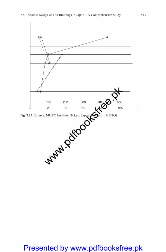
0 25 50 75 100 125
100 200 300 400 500
Fig. 7.13 (Source: MUTO Institute, Tokyo, Japan. Professor: MUTO)
7.5 Seismic Design of Tall Buildings in Japan – A Comprehensive Study 543
www.pdfbo
oksfr
ee.pk
Presented by www.pdfbooksfree.pk
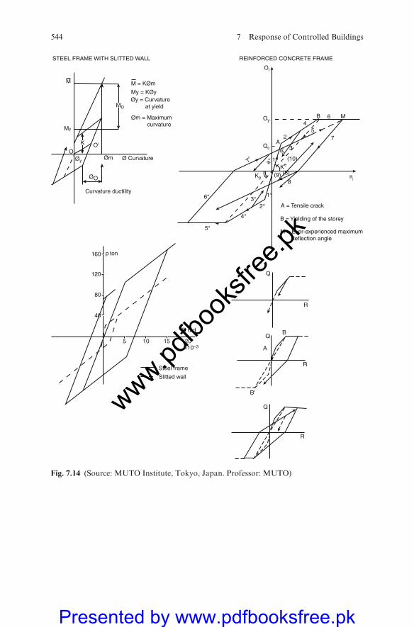
5 10 15 20×10–3
40
80
120
160 p ton
R rad
Steel frame
Slitted wall
Q
R
Q
R
QB
A
R
B'
STEEL FRAME WITH SLITTED WALL
M
My
Øy
OO'
Øm
ØO
Ø Curvature
Curvature ductility
M = KØm
My = KØyØy = Curvature at yield
Øm = Maximum curvature
A = Tensile crack
B = Yielding of the storey
M = Ever-experienced maximum deflection angle
REINFORCED CONCRETE FRAME
Oi
Oy
Qc
Kp
B 6 M
75
4
2A
1
3
Ke
3°2°
1°
a°
9°
4°
5°
6°
(10)
(9) (8)
8
7°
Rj
K
Mo
Fig. 7.14 (Source: MUTO Institute, Tokyo, Japan. Professor: MUTO)
544 7 Response of Controlled Buildings
www.pdfbo
oksfr
ee.pk
Presented by www.pdfbooksfree.pk
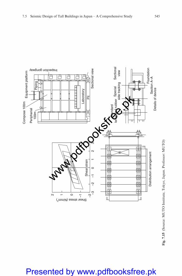
–3–2
–10
She
ar s
trai
n
Shear stress (N/mm2)
2 1 0 –1 –21
2P
it
Fou
ndat
ion
Sec
tiona
l vie
w
Det
ails
of d
evic
eS
ectio
n A
–AD
istr
ibut
ion
arra
ngem
ent
Sta
ndar
dla
min
ated
rub
ber
Spe
cial
si
de tr
acki
ngS
ectio
nal
view
Com
pose
100
mE
quip
men
t pla
tform
Pip
ing
Per
iphe
rial
100m
Inspection gongway
Labo
rato
ry
3
Fig.7.15(Source:MUTO
Institute,Tokyo,Japan.Professor:MUTO)
7.5 Seismic Design of Tall Buildings in Japan – A Comprehensive Study 545
www.pdfbo
oksfr
ee.pk
Presented by www.pdfbooksfree.pk
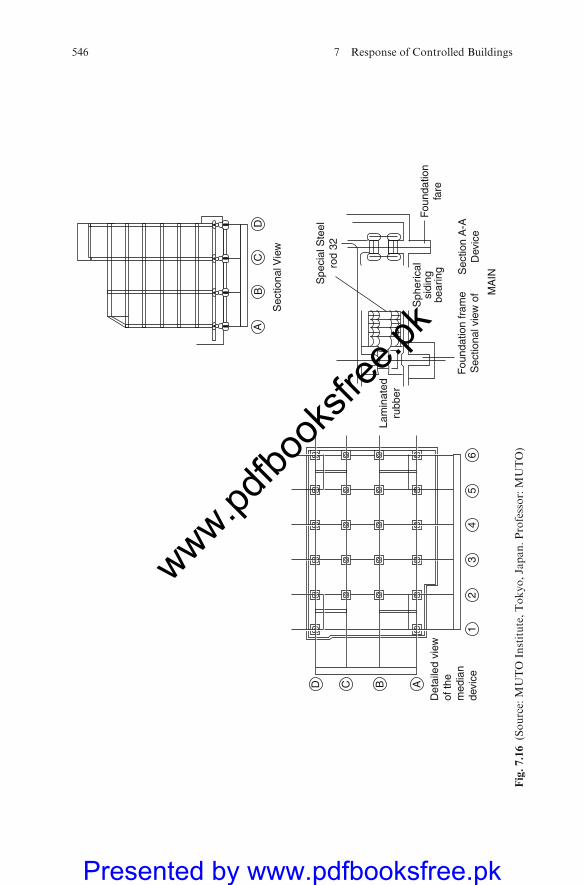
65
43
21
A
Det
aile
d vi
ewof
the
med
ian
devi
ce
BCD
AB
Sec
tiona
l Vie
w
Spe
cial
Ste
elro
d 32
Fou
ndat
ion
fare
Sec
tion
A-A
Dev
ice
Fou
ndat
ion
fram
eS
ectio
nal v
iew
of M
AIN
Sph
eric
alsi
ding
bear
ing
Lam
inat
edru
bber
CD
Fig.7.16(Source:MUTO
Institute,Tokyo,Japan.Professor:MUTO)
546 7 Response of Controlled Buildings
www.pdfbo
oksfr
ee.pk
Presented by www.pdfbooksfree.pk
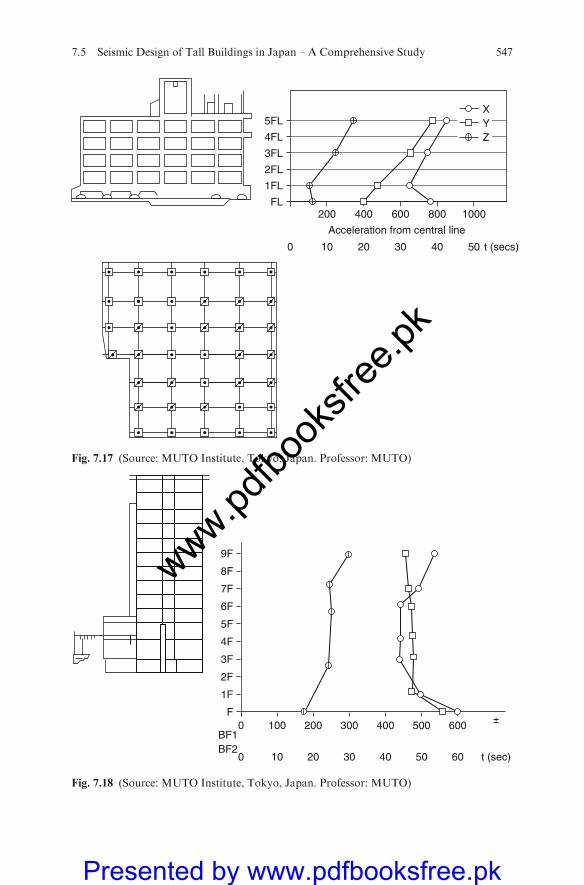
200 400
Acceleration from central line
600 800 1000
100 20 30 40 50 t (secs)
5FL
4FL
3FL
2FL
1FL
FL
XYZ
Fig. 7.17 (Source: MUTO Institute, Tokyo, Japan. Professor: MUTO)
100BF1
0 200 300 400 500 600
10BF2
0 20 30 40 50 60 t (sec)
±
5F
8F
9F
7F
6F
4F
3F
2F
1F
F
Fig. 7.18 (Source: MUTO Institute, Tokyo, Japan. Professor: MUTO)
7.5 Seismic Design of Tall Buildings in Japan – A Comprehensive Study 547
www.pdfbo
oksfr
ee.pk
Presented by www.pdfbooksfree.pk
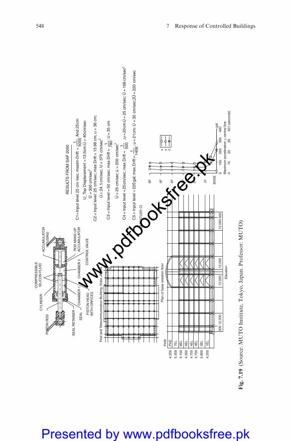
Pos
t and
Tel
ecom
mun
icat
ion
Bui
ldin
g, K
obe
JAPA
N
PIS
TON
RO
D
CY
LIN
DE
R
PIS
TON
HE
AD
WIT
H O
RF
ICE
S
SE
AL
RE
TAIN
ER
SE
AL
CH
AM
BE
R 1
CH
AM
BE
R 2
CO
NT
RO
L V
ALV
E
RO
D M
AK
E-U
PA
CC
UM
ULA
TOR
AC
CU
MU
LATO
RH
OU
SIN
G
CO
MP
RE
SS
IBLE
SIL
ICO
N F
LUID
Ele
vatio
nM
axim
um a
ccel
erat
ion
+ c
entr
al li
ne
4.20
0
PH
RP
lan
of b
ase
isol
atio
n flo
or
000
12.0
0012
.000
12.0
0012
.000
000
PH
2
7EL
6EL
5EL
4EL
3EL
2EL
1EL
5.30
0
4.15
0
4.35
0
4.75
0
4.25
0
4.75
0
5.80
0
5F6F 4F 3F 2F 1F
0 010
2030
t (se
cond
s)40
100
200
300
400ga
lB
AS
E
x y z
RE
SU
LTS
FR
OM
SA
P 2
000
C1=
Inpu
t lev
el 2
5 cm
/sec
; max
im-D
rift
=1
5000
And
25
cm
U_T
op D
ispl
acem
ent =
13.5
cm;Ú
= 4
0cm
/sec
Ü =
300
cm
/sec
2
Ú =
25
cm/s
ec; ü
= 2
00 c
m/s
ec2
Ú =
24.
5 c
m/s
ec; U
= 3
75 c
m/s
ec2
C2
= In
put l
evel
: 25
cm
/sec
; max
.Drif
t = 1
3.98
cm
; u =
36
cm;
; U =
35
cm
C3
= In
put l
evel
= 5
0 c
m/s
ec; m
ax.D
rift =
1 780
C5
= In
put l
evel
= 2
20 g
al; m
ax.D
rift =
; u =
21
cm; Ú
= 3
0 c
m/s
ec;Z
Ü =
220
cm
/sec
114
06
C4
= In
put l
evel
= 2
5cm
/sec
; max
Drif
t =1 500
;u =
20
cm Ú
= 2
5 cm
/sec
; Ü =
168
cm
/sec
2
CA
SE
ST
UD
Y C
I
Fig.7.19(Source:MUTO
Institute,Tokyo,Japan.Professor:MUTO)
548 7 Response of Controlled Buildings
www.pdfbo
oksfr
ee.pk
Presented by www.pdfbooksfree.pk
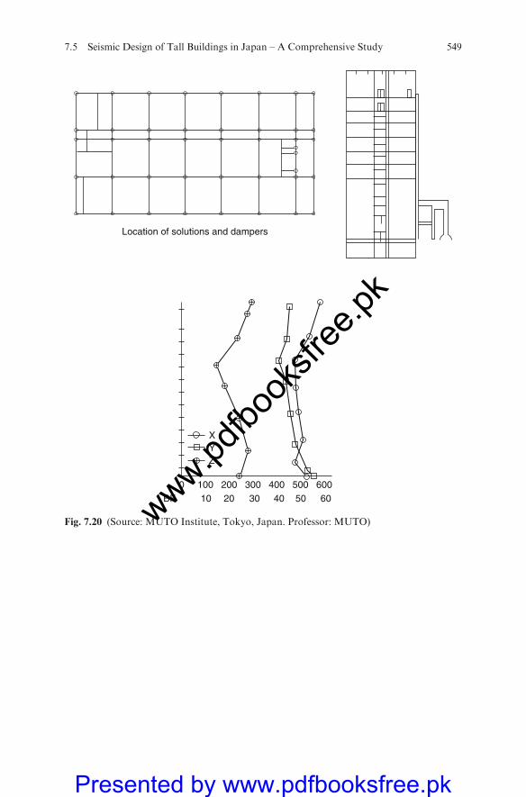
100BF 10 20 30 40 50 60
0 200 300
Location of solutions and dampers
400 500 600
XYZ
Fig. 7.20 (Source: MUTO Institute, Tokyo, Japan. Professor: MUTO)
7.5 Seismic Design of Tall Buildings in Japan – A Comprehensive Study 549
www.pdfbo
oksfr
ee.pk
Presented by www.pdfbooksfree.pk
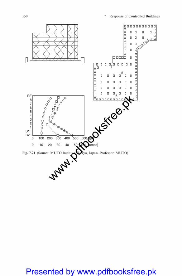
0 100 200 300 400 500 600
0
B2FB1F
12345678
RF
10 20 30 40 50 60
gal
73
5
6
t(secs)
Fig. 7.21 (Source: MUTO Institute, Tokyo, Japan. Professor: MUTO)
550 7 Response of Controlled Buildings
www.pdfbo
oksfr
ee.pk
Presented by www.pdfbooksfree.pk
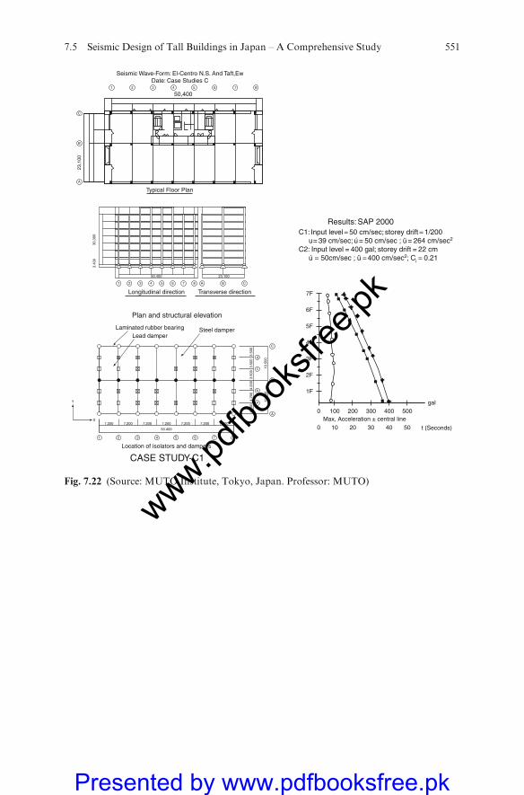
5F
6F
7F
4F
3F
2F
1F
0 100 200 300 400 500
0 10 20 30 40 50
gal
Max, Acceleration ± central line
Longitudinal direction Transverse direction
50.400 23.100
30,3
003.
400
1 2 3 4 5 6 7 8 A CB
Typical Floor Plan
50,400
23,1
00
2 3 4 5 6 7 81
C
B
A
Seismic Wave-Form: El-Centro N.S. And Taft,EwDate: Case Studies C
t (Seconds)
Results: SAP 2000C1: Input level = 50 cm/sec; storey drift = 1/200 u = 39 cm/sec; ú = 50 cm/sec ; ü = 264 cm/sec2
C2: Input level = 400 gal; storey drift = 22 cm ú = 50cm/sec ; ü = 400 cm/sec2; Ci = 0.21
1 2 3 4 5 6 7 8
a
A
B
C
b
c
d
Y
X
50.400
Laminated rubber bearing
Plan and structural elevation
Location of isolators and dampers
Lead damperSteel damper
7.200 7.200 7.200 7.200 7.200 7.200 7.200
4.20
04.
200
10.5
00
4.20
03.
500
3.50
0
12.6
00
3.50
0
CASE STUDY-C1
Fig. 7.22 (Source: MUTO Institute, Tokyo, Japan. Professor: MUTO)
7.5 Seismic Design of Tall Buildings in Japan – A Comprehensive Study 551
www.pdfbo
oksfr
ee.pk
Presented by www.pdfbooksfree.pk
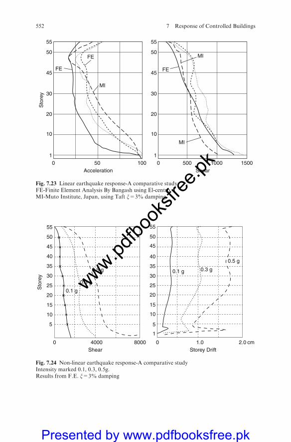
55
50
45
30
20
10
10 50 100
55
50
45
30
20
10
10 500 15001000
FE
MI
MIFE
FE
Acceleration Shear
Sto
rey
MI
Fig. 7.23 Linear earthquake response-A comparative studyFE-Finite Element Analysis By Bangash using El-centroMI-Muto Institute, Japan, using Taft x=3% damping
5
1
10
15
20
25
30
35
40
45
50
55
5
10
15
20
25
30
35
40
45
50
55
0 4000 8000 0 1.0 2.0 cm
Sto
rey
Shear Storey Drift
0.1 g
0.1 g
0.3 g
0.3 g
0.5 g
0.5 g
Fig. 7.24 Non-linear earthquake response-A comparative studyIntensity marked 0.1, 0.3, 0.5g.Results from F.E. x=3% damping
552 7 Response of Controlled Buildings
www.pdfbo
oksfr
ee.pk
Presented by www.pdfbooksfree.pk
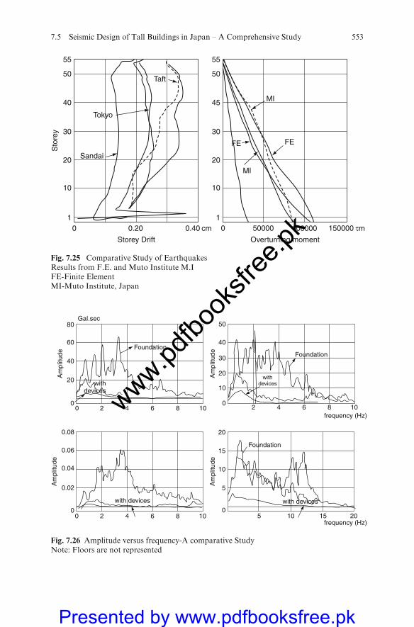
55
50
40
30
20 Sandai
Tokyo
Sto
rey
10
10 0.20
Storey Drift Overturning moment
0.40 cm
55
50Taft
45
30
20
FE
MI
FE
MI
10
10 50000 150000 τm100000
Fig. 7.25 Comparative Study of EarthquakesResults from F.E. and Muto Institute M.IFE-Finite ElementMI-Muto Institute, Japan
0
withdevices
with devices
withdevices
with devices
20 4 6 8 10 2 4 6 8 10
5 10 15 2020 4 6 8 10
20
40
0.08
0.06
0.04
0.02
0
60
80
0
20
10
20
15
10
5
0
30
40
50
Foundation
Foundation
Foundation
frequency (Hz)
frequency (Hz)
Am
plitu
de
Am
plitu
de
Am
plitu
de
Am
plitu
de
Gal.sec
Fig. 7.26 Amplitude versus frequency-A comparative StudyNote: Floors are not represented
7.5 Seismic Design of Tall Buildings in Japan – A Comprehensive Study 553
www.pdfbo
oksfr
ee.pk
Presented by www.pdfbooksfree.pk

damping of 0.03 is kept constant taking into consideration the soil–structure
interaction effects.Then it is necessary to check Fourier spectrum in each direction for the SMB
building with and without seismic devices using Program ETAB. Plate 7.15
shows these results.It is concluded that vertical acceleration is important and cannot now be
ignored. Since the SMB building is not actually in the Kobe region, the building
is safe and the existing design features are adequate even if the vertical accel-
eration parameters are included. In the Kobe region this type of building would
receive superficial damage but would not collapse due to specific layout tech-
niques adopted by the Muto Institute, Japan.
554 7 Response of Controlled Buildings
www.pdfbo
oksfr
ee.pk
Presented by www.pdfbooksfree.pk
Chapter 8
Seismic Criteria and Design Examples Based
on American Practices
8.1 General Introduction
This chapter briefly contains the design criteria provided in UBC-97. A table is
provided for various structural systems and is followed by the structural design
requirements for framing systems, performance categories, building configura-tions, including plan and vertical structural irregularities. As action is given on
combination of load effects, it became necessary to give the American views ondeflection and drift limits. This is followed by equivalent lateral force procedure,
period determination and seismic base shear. Vertical distribution of seimicforces and horizontal base shear distribution, torsion and overturning moments
are fully described and supported by design equations. NextP� D effects, modal
forces, deflection and drifts are given due consideration. Soil– structure interac-
tion effects given earlier in the text are briefly mentioned to remind the designerthat it necessarily has to be dealt with. They are described in Chap. 6.
This chapter gives away design examples based on the criteria given in
UBC-97.
8.2 Structural Design Requirements for Structures
8.2.1 Introduction to the Design Basis
The seismic analysis and design procedures to be used in the analysis anddesign of structures and their components shall be as prescribed in various
codes. The design ground motions can occur along any direction of a struc-
ture. The design seismic forces and their distribution over the height of the
structure shall be established by a specific code and the corresponding internalforces in the members of the structure shall be determined using a linearly
elastic model. An approved alternative procedure may be used to establish theseismic forces and their distribution, in which case the corresponding internal
forces and deformations in the members shall be determined using a theore-tical model.
M.Y.H. Bangash, Earthquake Resistant Buildings,DOI 10.1007/978-3-540-93818-7_8, � M.Y.H. Bangash 2011
555
www.pdfbo
oksfr
ee.pk
Presented by www.pdfbooksfree.pk
Individual members shall be designed and sized for the shears, axial forces
and moments determined in accordance with these provisions, and connectionsshall develop the strength of the connected members or the forces. The founda-tion shall be designed to accommodate the forces developed or the movement
imparted to the structure by the design groundmotions. In the determination ofthe foundation design criteria, special recognition shall be given to the dynamicnature of the forces, the expected ground motions and the design basis forstrength and energy dissipation capacity of the structure. The foundations can
be flexible or rigid. In the layout the foundations shall have the isolators care-fully arranged to offset damaging seismic forces. Themost comprehensive workis given on numerical modelling in the author’s book on Earthquake Resisting
Buildings, published by Springer-Verlag, Germany.
8.3 Drift Determination and P–D Effects
Storey drifts and, where required, member forces and moments due to P� Deffects shall be determined in accordance with this section.
8.3.1 Storey Drift Determination
The design storey drift shall be computed as the difference between the deflec-tions at the top and bottom of the storey under consideration. The deflections of
level x and the centre of the mass dx (in or mm) shall be determined inaccordance with the following equation:
dx ¼ Cddxc (8:1)
where
Cd¼ the deflection amplification factordxc ¼ the deflection determined by an elastic analysis (in or mm).
Where applicable, the design storey drift D (in or mm) shall be increased bythe incremental factor relating to the P� D effects.
8.4 P–D Effects
P� D effects on storey shears and moments the resulting member forces and
moments and the storey drifts induced by these effects are not required to beconsidered when the stability coefficient y, as determined by the followingequation, is equal to or less than 0.10:
556 8 Seismic Criteria and Design Examples
www.pdfbo
oksfr
ee.pk
Presented by www.pdfbooksfree.pk
y ¼ PxDð Þ= VxhsxCdð Þ (8:2)
where
Px ¼ the total vertical design load above level x (kip or kN); when circulatingthe vertical design load for purpose of determining P� D, the individualload factors need not exceed 1.0
D ¼ the design storey drift occurring simultaneously with Vx (in or mm)Vx ¼ the seismic shear force acting between level x and x�1 (kip or kN)hsx ¼ the storey height below level x (ft or m)Cd= the deflection amplification factor
The stability coefficient y shall not exceed ymax, determined as follows:
ymax ¼ 0:5=ðbCdÞ � 0:25 (8:3)
8.5 Modal Forces, Deflection and Drifts
The modal force Fxm at each level shall be determined by the following
equations:
Fxm ¼ CvxmVm (8:4)
8.6 Soil–Concrete Structure Interaction Effects
8.6.1 General
The provisions set forth in this section may be used to incorporate the effects of
soil–concrete structure interaction in the determination of the design earth-quake forces and the corresponding displacement of the building. The use of
these provisions will decrease the design values of the base shear lateral forcesand overturning moments but may increase the computed values of the later
displacements and the secondary forces associated with the P� D effects. Theprocedure is given elaborately in Chap. 6.
8.7 Equivalent Lateral Forces Procedure
The following provisions are supplementary to those presented above.
8.7 Equivalent Lateral Forces Procedure 557
www.pdfbo
oksfr
ee.pk
Presented by www.pdfbooksfree.pk
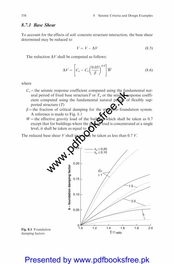
8.7.1 Base Shear
To account for the effects of soil–concrete structure interaction, the base sheardetermined may be reduced to
V ¼ V� DV (8:5)
The reduction DV shall be computed as follows:
DV ¼ Cs � Cs0:05
b
� �0:4" #
W (8:6)
where
Cs¼ the seismic response coefficient computed using the fundamental nat-ural period of fixed base structureT or Ta or the seismic response coeffi-cient computed using the fundamental natural period of flexibly sup-ported structure (T)
b¼ the fraction of critical damping for the structure–foundation system.A reference is made to Fig. 8.1
W¼ the effective gravity load of the building which shall be taken as 0.7except that for buildings where the gravity load is concentrated at a singlelevel, it shall be taken as equal to W.
The reduced base shear V shall in no case be taken as less than 0.7 V.
Β –
fou
nd
atio
n d
amp
ing
fac
tor
1.5
2.0
5
H.r≤ 1
02.01.21.0 1.4 1.6 1.8
0.25
0.20
0.15
0.10
0.05
Δv ≤ 0.10Δv ≥ 0.20
T/ T ratioFig. 8.1 Foundationdamping factors
558 8 Seismic Criteria and Design Examples
www.pdfbo
oksfr
ee.pk
Presented by www.pdfbooksfree.pk
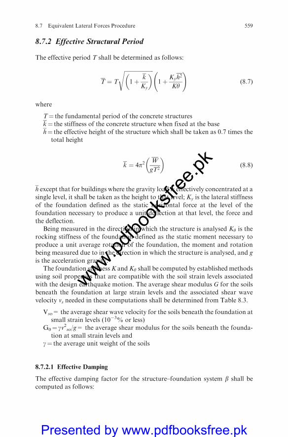
8.7.2 Effective Structural Period
The effective period T shall be determined as follows:
T ¼ T
ffiffiffiffiffiffiffiffiffiffiffiffiffiffiffiffiffiffiffiffiffi1þ k
Ky
� �s1þ Kyh2
Ky
!(8:7)
where
T¼ the fundamental period of the concrete structuresk¼ the stiffness of the concrete structure when fixed at the baseh¼ the effective height of the structure which shall be taken as 0.7 times the
total height
k ¼ 4p2W
gT2
� �(8:8)
h except that for buildings where the gravity load is effectively concentrated at asingle level, it shall be taken as the height to that level; Ky is the lateral stiffnessof the foundation defined as the static horizontal force at the level of thefoundation necessary to produce a unit deflection at that level, the force andthe deflection.
Being measured in the direction in which the structure is analysed Ky is therocking stiffness of the foundation defined as the static moment necessary toproduce a unit average rotation of the foundation, the moment and rotationbeing measured due to in the direction in which the structure is analysed, and gis the acceleration gravity.
The foundation stiffnessK andKy shall be computed by established methodsusing soil properties that are compatible with the soil strain levels associatedwith the design earthquake motion. The average shear modulus G for the soilsbeneath the foundation at large strain levels and the associated shear wavevelocity vs needed in these computations shall be determined from Table 8.3.
Vso= the average shear wave velocity for the soils beneath the foundation atsmall strain levels (10�3% or less)
G0¼ gv2so/g= the average shear modulus for the soils beneath the founda-tion at small strain levels and
g¼ the average unit weight of the soils
8.7.2.1 Effective Damping
The effective damping factor for the structure–foundation system b shall becomputed as follows:
8.7 Equivalent Lateral Forces Procedure 559
www.pdfbo
oksfr
ee.pk
Presented by www.pdfbooksfree.pk
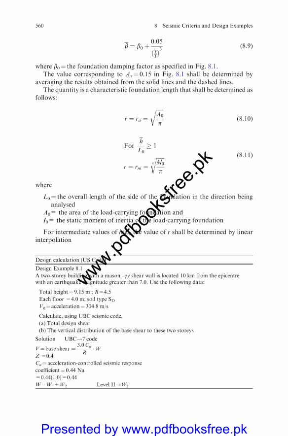
b ¼ b0 þ0:05
ðTTÞ3
(8:9)
where b0¼ the foundation damping factor as specified in Fig. 8.1.The value corresponding to Av¼ 0.15 in Fig. 8.1 shall be determined by
averaging the results obtained from the solid lines and the dashed lines.The quantity is a characteristic foundation length that shall be determined as
follows:
r ¼ ra ¼ffiffiffiffiffiffiA0
p
r(8:10)
Forh
L0� 1
r ¼ rm ¼ffiffiffiffiffiffi4l0
p4
r (8:11)
where
L0¼ the overall length of the side of the foundation in the direction beinganalysed
A0= the area of the load-carrying foundation andI0= the static moment of inertia of the load-carrying foundation
For intermediate values of h/L0 the value of r shall be determined by linearinterpolation
Design calculation (US Code)
Design Example 8.1
A two-storey building with a mason –gy shear wall is located 10 km from the epicentrewith an earthquake magnitude greater than 7.0. Use the following data:
Total height¼ 9.15 m ; R=4.5
Each floor =4.0 m; soil type SDVg¼ acceleration¼ 304.8 m/s
Calculate, using UBC seismic code,
(a) Total design shear
(b) The vertical distribution of the base shear to these two storeys
Solution UBC!7 code
V¼ base shear ¼ 3:0Ca
R�W
Z =0.4
Ca¼ acceleration-controlled seismic response
coefficient¼ 0.44 Na
=0.44(1.0)=0.44
W=W1+W2 Level II!W2
560 8 Seismic Criteria and Design Examples
www.pdfbo
oksfr
ee.pk
Presented by www.pdfbooksfree.pk
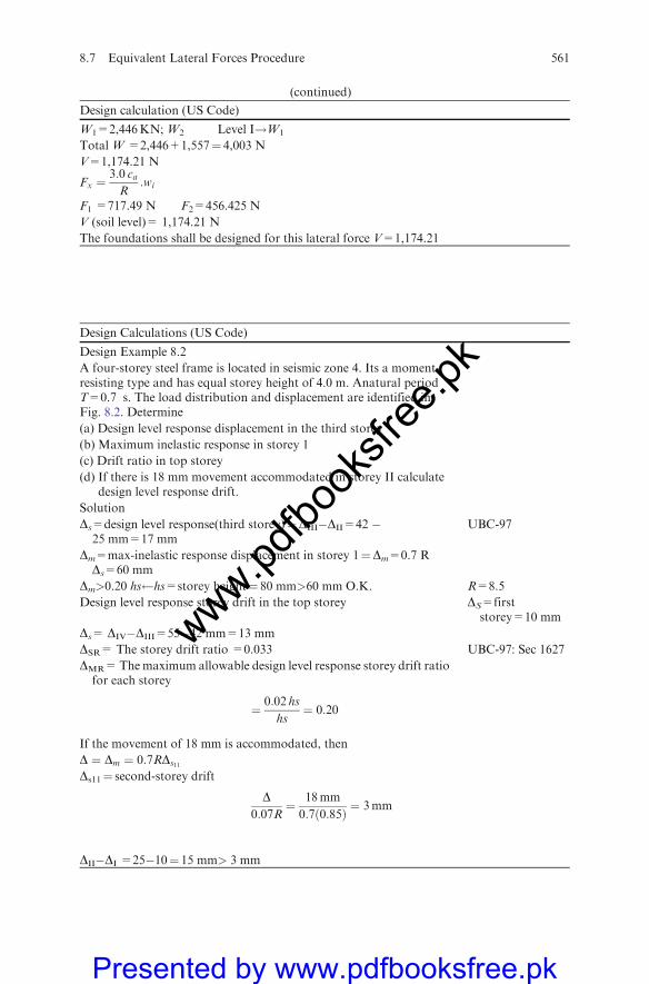
(continued)
Design calculation (US Code)
W1=2,446KN; W2 Level I!W1
Total W =2,446+1,557¼ 4,003 N
V=1,174.21 N
Fx ¼3:0 caR
:wi
F1 =717.49 N F2=456.425 N
V (soil level)= 1,174.21 N
The foundations shall be designed for this lateral force V=1,174.21
Design Calculations (US Code)
Design Example 8.2
A four-storey steel frame is located in seismic zone 4. Its a moment-resisting type and has equal storey height of 4.0 m. Anatural periodT=0.7 s. The load distribution and displacement are identified inFig. 8.2. Determine
(a) Design level response displacement in the third storey
(b) Maximum inelastic response in storey 1
(c) Drift ratio in top storey
(d) If there is 18 mm movement accommodated in storey II calculatedesign level response drift.
Solution
Ds=design level response(third storey)¼DIII�DII=42 �25 mm=17 mm
UBC-97
Dm=max-inelastic response displacement in storey 1¼Dm=0.7 RDs=60 mm
Dm>0.20 hs hs=storey height¼ 80 mm>60 mm O.K. R=8.5
Design level response storey drift in the top storey DS=firststorey=10 mm
Ds= DIV�DIII=55�42 mm=13 mm
DSR= The storey drift ratio =0.033 UBC-97: Sec 1627
DMR=Themaximum allowable design level response storey drift ratiofor each storey
¼ 0:02 hs
hs¼ 0:20
If the movement of 18 mm is accommodated, then
D ¼ Dm ¼ 0:7RDs11
Ds11¼ second-storey drift
D0:07R
¼ 18mm
0:7ð0:85Þ ¼ 3mm
DII�DI =25�10¼ 15 mm> 3 mm
8.7 Equivalent Lateral Forces Procedure 561
www.pdfbo
oksfr
ee.pk
Presented by www.pdfbooksfree.pk
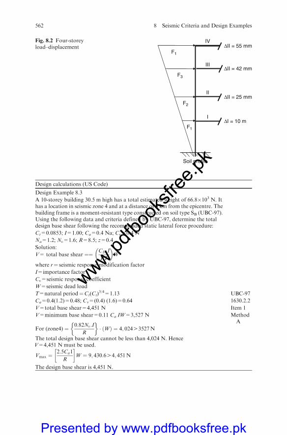
Design calculations (US Code)
Design Example 8.3
A 10-storey building 30.5 m high has a total estimated weight of 66.8�103 N. Ithas a location in seismic zone 4 and at a distance of 5 km from the epicentre. Thebuilding frame is a moment-resistant type constructed on soil type SB (UBC-97).Using the following data and criteria defined by UBC-97, determine the totaldesign base shear following the recommended static lateral force procedure:
Ct=0.0853; I=1.00; Ca=0.4 Na; Cu=0.4 N
Na=1.2; Nu=1.6; R=8.5; z=0.4
Solution:
V= total base shear ¼¼ CD:I
RT
� �W
where r¼ seismic response modification factor
I=importance factor
Cu=seismic response coefficient
W=seismic dead load
T=natural period¼Ct(Ct)3/4=1.13 UBC-97
Ca=0.4(1.2)=0.48; Cv=(0.4) (1.6)=0.64 1630.2.2
V=total base shear=4,451 N Item 1
V=minimum base shear=0.11 Ca IW=3,527 N MethodA
For (zone4) ¼ 0:82Nu:I
R
� �� ðWÞ ¼ 4; 02443527N
The total design base shear cannot be less than 4,024 N. HenceV=4,451 N must be used.
Vmax ¼2:5Ca1
R
� �W ¼ 9; 430:644; 451N
The design base shear is 4,451 N.
F1
ΔI = 10 m
ΔII = 25 mm
ΔII = 42 mm
ΔII = 55 mm
F2
F3
F1
I
II
III
IV
Soil profile
Fig. 8.2 Four-storeyload–displacement
562 8 Seismic Criteria and Design Examples
www.pdfbo
oksfr
ee.pk
Presented by www.pdfbooksfree.pk

Design calculations (US Code)
Design Example 8.4
The horizontal stiffness of a single isolator is defined by KH=GA,whereG is the shear modulus of a rubber,A is the full cross-sectionalarea of the pad. And tr is the total thickness of the pad rubber.Assuming the diameter of the isolator=240 0 and the designdisplacement is 11.430 0, calculate the value of the period TD.
tr=1.50 0 0 note 1 inch=25.4mm
g=38.4 ; T=0.73 s
DD=design displacement=11.430 0
G=7.35 Kips/in2
Solution
A ¼ pf2
4¼ pð24Þ2
4¼ 425 in2
Total rubber thickness ¼ D
tr¼ 11:43
1:50¼ 7:6
KH ¼7:35ð452Þ
384¼ 8:65Kip=in
TD ¼ 2:5
ffiffiffiffiffiffiffiffiffi7:35
8:65
r¼ 2:3 s
TD � 3Tfixedbase ¼ 3ð0:7Þ ¼ 2:1
Hence TD=2.3>2.1 OK.
The isolator initial parameter OK.
8.7 Equivalent Lateral Forces Procedure 563
www.pdfbo
oksfr
ee.pk
Presented by www.pdfbooksfree.pk

www.pdfbo
oksfr
ee.pk
Presented by www.pdfbooksfree.pk
Chapter 9
Design of Structural Elements Based on Eurocode 8
9.1 Introduction
This chapter covers only the requirements related to Eurocode 8. Other codes,for comparison, currently in existence is briefly given. Prior to the designcalculations an emphasis is placed on the types of superstructure and structuralsystems, classifications of the seismic zones. A preference is given to the EC8requirements in this chapter. At the time of writing this chapter calculationshave been attempted to design structural elements using EC8. Some relevantequations are given and they have been referred to while carrying out design ofstructural elements. The reader is advised to Study Chaps. 2, 4 and 5 as well andgrab the basic methods and related calculations.
9.2 Existing Codes
A reference is made to Chap. 2 regarding existing codes. The following list covermore or less the codes followed by other countries in case the designers need acomparative study of seismic code requirements:
Algeria Earthquake Resistance Regulations RPA (2002)
Australia Minimum Design Load on Structures AS1170 Part 4 (1996)
Austria Design Loads in Building ONoRmB4015 Part 1 (1999)
Bulgaria Code for Design of Buildings and Structures in Seismic Regions(1996)
Canada National Building Code of Canada (1996)
Chile –
China Peoples Republic of Code for Seismic Design of Buildings (2001)
Colombia –
Costa Rica –
Croatia Similar to Yugoslavia and revised in 1999
Cuba –
Dominican Republic Provisional and Recommendations for Seismic Analysis ofStructures (2004)
M.Y.H. Bangash, Earthquake Resistant Buildings,DOI 10.1007/978-3-540-93818-7_9, � M.Y.H. Bangash 2011
565
www.pdfbo
oksfr
ee.pk
Presented by www.pdfbooksfree.pk

Ecuador Manual de adise n de Esstructureas sismo. Resistentes paratusvs guil (2000)
Egypt Regulations for Earthquake-Resistant Design of Buildings inEgypt (1996)
El Salvador –
Ethiopia –
France NF Po6013 (AFNOR Buildings) (1997)
Germany German Standard Din 4144 Building in German EarthquakeArea (2002)
Ghana Code for the Seismic Design of Concrete Structure (1990)
Greece Greek code for Seismic-Resistant Structures EAK 2000 (2000)
Hungary Dimensioning Directives for Seismic Effects, MI-04.133-81-Now Eurocode 8 (2005)
India Criteria for Earthquake Design of structures, Part 1, BIS (2002)IS 1893-1 (2002)
Indonesia –
Iran Iranian Code for Seismic-Resistant Design of Buildings (1998)
Israel Design Provision for Earthquake Resistance of Structures SI413 (1998)
Italy Technical Rules for Construction in Seismic Zones (2002), NowEurocode 8 (2005)
Japan Earthquake-Resistant Design Method for Building Part (2)2000 (other versions)
Jordan Jordan Code for Loads and Forces (1990)
Korea Building Code for Structural Regulations (2000)
Macedonia –
Mexico –
Nepal Nepal National Building Code NBC (2004)
New Zealand General Structural Design and Design Loadings for BuildingsNZS4203 (2004)
Nicaragua –
Norway Following the Eurocode 8 (2005)
Panama –
Peru –
Philippines –
Portugal Following the Eurocode 8 (2005)
Romania Seismic Building Code (2000), now following the Eurocode 8(2005)
Russian Federation Seismic Building Code 2000
Slovenia Following the Eurocode 8 (2005)
Spain Following the Eurocode 8 (2005)
Switzerland Standard STA 160, Action on Structures (2003), nowFollowing the Eurocode 8 (2005)
Chinese Taiwan Building Code for Earthquake-Resistant Structures (2002)
Thailand –
Turkey Specification for Structures to be Built in Disaster Areas (2000)
United States of America Minimum Design Loads for Building and Structures ASCE-7(2002)
566 9 Design of Structural Elements Based on Eurocode 8
www.pdfbo
oksfr
ee.pk
Presented by www.pdfbooksfree.pk
Venezuela –
Yugoslavia Following the Eurocode 8 (2005)
Eurocode 8 Design Provisions for Earthquake Resistance of Structures (2005)
ISO 3010 International Standard Base for Design of Structures: SeismicActions (2001)
(former) Yugoslavia Code of Technical Regulations for the Design andConstruction of Building in Seismic Regions (1981)
9.2.1 Explanations Based on Clause 4.2.3 of EC8 RegardingStructural Regularity. A Reference is Made to Eurocode 8:Part 1 – Design of Structures for Earthquake Resistance
Note: This brief is refered to the extended version of clause 4.2.3 of the code
(i) Criteria for regularity in plan:
The slenderness ratio l ¼ Lmax=Lmin � 4
where Lmax = larger dimensions in plan; Lmin = smaller dimensions in plan inorder to meet the above condition:
The total length of the building ¼ 5m; the width of the building ¼ 16m
One has divided the total length (5 m) of the building into three separateindependent portions, two external units of 42 m = 84 m; and the centralunit of 21 m=21m, thus totalling 10mwith a clear gap between the units; 4m has been left so that the earthquake force on each unit will not affect theadjacent one due to collision as explained in this text. The overall area is114� 21m. In our case, l ¼ 42=16 ¼ 2:6554.
So, it satisfies the criteria for regularity in plan:
(ii) Criteria for regularity in elevation:If the building is regular in plan, with slight deviation in central unit, it
will satisfy the criteria for elevation in plan.(iii) Criteria for well-distributed and relatively rigid cladding:
The criteria is satisfied by providing with well-distributed rigid claddingon the roof and vertical sides.
9.2.2 Seismological Actions (Refer Clause 3.2 of EC8)
The construction area is in the earthquake zone of ‘strong’ intensity which isequivalent to the Modified Mercalli (MM) scale between VII and VIII andRicher scale between 6.2 and 6.8Assumed: in our case, horizontal ground acceleration = 0.1g
9.2 Existing Codes 567
www.pdfbo
oksfr
ee.pk
Presented by www.pdfbooksfree.pk

For most of the application of EN 1998, the hazard is described in terms of asingle parameter, i.e. the value of the reference peak ground acceleration ontype A ground, agR.
The reference peak ground acceleration, chosen by the National Authoritiesfor each seismic zone, corresponds to the reference return period of the seismicaction for the no-collapse requirement (or equivalently the reference probabilityof exceedance in 50 years) chosen by the National Authorities (see Chap. 14).An importance factor = 1.0 is assigned to this reference period.
Low sensitivity is recommended
(i) when the design ground acceleration on type A ground, ag � 0:08 g or(ii) when the product ag � S � 0:1 g
In the analysis ag is the same as ug or €Xg. This is convenient in the analyticalformulation.
The basic representation of the seismic action is given in Clause 3.2.2 usingground type based on Table 3.1 of EC8.
9.3 Avoidance in the Design and Construction in Earthquake Zones:
Contributing Factors Responsible for Collapse Conditions
Many buildings collapse during earthquakes due to many contributing factors.Prior to the design of buildings, it is necessary to
1. Avoid soft storey ground floors: Walls existing in the upper floors are omitted inthe ground floor but replaced by columns. This means the ground floor is soft inthe horizontal direction. In such constructions the columns receive damage dueto the cyclic displacements between the building upper parts and the vibrating ormoving soil. A storey mechanism sometimes exists by the developing plastichinges at the top and the bottom of columns with a large concentration ofplastic deformations at their ends. Hence the collapse inevitably occurs.
2. Avoid soft storey upper floors: Once the lateral bracing is weakened, omittedaltogether or the horizontal resistance is substantially reduced above a particularfloor, a dangerous sway mechanism occurs and hence the collapse is inevitable.
3. Avoid a symmetric bracing:When the centre of the buildingmass and the centreof resistance do not coincide, definitely twist occurs. This develops torsion in thehorizontal plane about the centre of the stiffness. Great relative displacementoccurs between the bottom and top of the columns in particular, by keepingthem far apart from the centre of stiffness. Failure normally occurs.
4. Avoid bracing offsets: Horizontal bracing offsets in-plane at the bottom planor out-of-plane at the top plan do cause position of the bracing changes fromone storey to another, thereby developing bending moments and shearforces. They, in the case of being continuous, definitely reduce seismicresistance. Bracing offsets must be avoided.
568 9 Design of Structural Elements Based on Eurocode 8
www.pdfbo
oksfr
ee.pk
Presented by www.pdfbooksfree.pk

5. Avoid columns and masonry walls mixed system: Mixed system of concretesteel column walls is unfavourable because
(a) Columns with slabs and beams develop frames with small horizontalstiffness than masonry wall.
(b) Failure of masonry wall due to seismic actions or deflection will beunable to carry gravity loads and inertia loads.
The collapse is inevitable.
6. Avoid bracing of frames with masonry infills: The frames structure is relativelyflexible and somewhat ductile. However, the unreinforced masonry is stiffand fragile. The two in combination will cause a damage scenario under theeffect of small deformations.
The combination of these two different incompatible construction does
perform poorly. Themasonry fails due to the shear or sliding diagonal cracks
that develop which indicates seismic failures. The framed structure will have
totally different performance as stated earlier. The failure is imminent.7. Avoid short columns: Shear is a problem in short columns. Shear failure
occurs reaching plastic moment capacity. Short columns are to be avoided.8. Avoid partially filled frames: The infill of parapet walls into a frame structure
without the addition of joints can cause shear failure like a short column. Aswaymechanism andP–D effect can occur when sufficient shear strength exists.
9.4 Superstructure and Structural Systems
9.4.1 Regularity
To offer a better resistance to earthquakes, the constructions should preferably
have simple forms on the one hand and a distribution of the masses and
rigidities as regular as possible in the plan and in elevation on the other hand.
9.4.2 Structural Systems
In general, the constructions should have lateral load-resisting system at least in
two horizontal directions. These systems should be arranged in order to
– take up sufficient vertical load enough to ensure their stability.– ensure a direct transmission of the forces to the foundations.– minimize the torsion action effects.
The lateral load-resisting systems should have a regular configuration and form
a continuous and coherent structural system as monolithic as possible. On the
other hand, this system should be sufficiently redundant in order to ensure an
important margin between the elastic limit and the rupture threshold of the
structure.
9.4 Superstructure and Structural Systems 569
www.pdfbo
oksfr
ee.pk
Presented by www.pdfbooksfree.pk

A Particular attention should be given to the design and execution of all the
connections, keeping in mind the effects of any failure at this level on behaviour
of the structure.
9.4.2.1 Reinforced Concrete Structures/Buildings
(a) Moment-resisting space frames without rigid masonry infill wallsThe concerned buildings should not exceed seven storeys or 23 m in
height in zone I low seismicity; six storeys or 20 m in height in zone II
moderate seismicity; two storeys or 8 m in height in zone III high seismicity.(b) Moment-resisting space frames with rigid masonry infill walls
Here the structure is composed uniquely of the frames capable of carry-
ing all forces due to the vertical and horizontal loads. The fill thickness shall
not exceed without loading 10 cm except for the exterior masonry infill
panels or for separating walls between two premises where a second wall of
5 cm is accepted on the interior side.The concerned building shall not exceed six storeys or 20 m height in
zones I and II and two storeys or 18 m in height in zone III.(c) Structural lateral load-resistant system composed of vertical load-carrying
shear walls in reinforced concrete.They arewalls andwall cum frames. The lateral casewill havewalls carrying
more than 20% vertical loads. The lateral loads are carried by the walls alone.(d) RC building entirely braced by RC core
Here the building is completely braced by the RC rigid core which carries
all horizontal loads.(e) Dual bracing systems composed of walls and frames with justification frame
wall interaction.
(i) Here the shear walls carry less than 20% of vertical loads.(ii) The horizontal loads are jointly carried by the shear walls and the
frames.(iii) The frames resist less than 25% of the storey shear in addition to
forces due to vertical loads.
(f) Moment-resisting frames system braced by RC shear walls. In this case theshear walls carry less than 20% of vertical loads plus total forces due tohorizontal loads.
The buildings are limited to 10 storeys or 33 mmaximum height. In zone III,
the frames shall have the capacity to resist not less than 25% of the storey shear
force due to the vertical loads.
Steel Structure or Buildings
(a) Structures or buildings braced with ordinary moment resisting the height ofall the buildings does not exceed five storeys or 17 m in height.
570 9 Design of Structural Elements Based on Eurocode 8
www.pdfbo
oksfr
ee.pk
Presented by www.pdfbooksfree.pk

(b) Ductile moment-resisting space frame systems. They alone resist the totalhorizontal loads.
(c) Structures or buildings braced by concentric braced frames.
The height of the building in this case is limited to five storeys or 17 m inheight.
The complete structure carries total vertical load.The moment-resisting space frames alone resist the total horizontal loads.
(d) Structures or buildings braced by the X-braced frame:In this system of a braced node, the axis of the diagonal, the beam and
the column are convergent to one point located in the centre of the node. Inthis type of frame only those diagonals which are in tension contribute tothe resistance and the dissipative behaviour.
(e) Structures or buildings with V-braced framesHere the beams of each braced frame are continuous and the point of the
intersection of the diagonal axis of the braced frame is located on the axis ofthe beam. The resistance and the capacity of dissipation are provided by thejoint participation of both the in-tension and in-compression diagonals.
(f) The moment-resisting frames and the braced frames should be designedto resist horizontal loads according to their relative rigidities considering theinteraction at all levels. The ductile moment-resisting frames should havethe capacity to alone resist not less than 25% of the global horizontal loads.
(g) Structural system braced with ductile frames and X-braced framesIn this system, the dual bracing system is a combination of ductile
moment-resisting space frames and concentric V-braced frames.(h) Vertical cantilever frame system
This category of structure with small degree of redundancy concernsessentially classical one-storey frames with rigid transversal beam andslender structure (tube) type where the resistant structural elements areessentially the columns located on the periphery of the structure.
These particular structures have a dissipative behaviour located uniquelyat the ends of the columns.
(i) Steel frame structure braced by diaphragmThese structures resist the seismic actions by the diaphragm effect of
vertical element (walls) and horizontal element (floors). The level of dissi-pative behaviour of these structures depends on the capacity of ductile shearresistance of these walls and floors that can be achieved with variousmaterials and technologies (cold-formed ribbed sheet, reinforced masonrywall, plain concrete or reinforced concrete wall, etc.
The walls should be fixed to the steel frame in order to consider theconnections as rigid.
(j) Steel frame structure braced by reinforced concrete coreSame definition as for reinforced concrete frames structural system.
(k) Steel frame structure braced by reinforced concrete shear wallsSame definition as for reinforced concrete frames structural system.
9.4 Superstructure and Structural Systems 571
www.pdfbo
oksfr
ee.pk
Presented by www.pdfbooksfree.pk
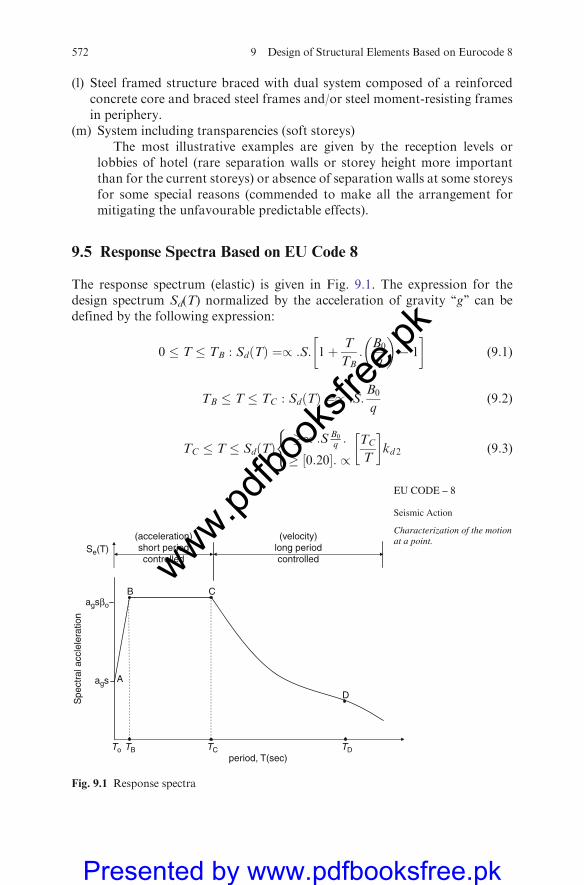
(l) Steel framed structure braced with dual system composed of a reinforcedconcrete core and braced steel frames and/or steel moment-resisting framesin periphery.
(m) System including transparencies (soft storeys)The most illustrative examples are given by the reception levels or
lobbies of hotel (rare separation walls or storey height more importantthan for the current storeys) or absence of separation walls at some storeysfor some special reasons (commended to make all the arrangement formitigating the unfavourable predictable effects).
9.5 Response Spectra Based on EU Code 8
The response spectrum (elastic) is given in Fig. 9.1. The expression for thedesign spectrum Sd(T) normalized by the acceleration of gravity ‘‘g’’ can bedefined by the following expression:
0 � T � TB : SdðTÞ ¼/ :S: 1þ T
TB:
B0
q
� �� 1
� �(9:1)
TB � T � TC : Sd Tð Þ ¼/ :S:B0
q(9:2)
TC � T � Sd Tð Þ�/ :S B0
q :
� 0:20½ �: /
(TC
T
� �kd 2 (9:3)
ags
Spe
ctra
l acc
lele
ratio
n
agsβo
(acceleration)short periodcontrolled
Se(T)(velocity)
long periodcontrolled
To TB TC TD
A
B C
D
period, T(sec)
Seismic Action
Characterization of the motionat a point.
EU CODE – 8
Fig. 9.1 Response spectra
572 9 Design of Structural Elements Based on Eurocode 8
www.pdfbo
oksfr
ee.pk
Presented by www.pdfbooksfree.pk

TD�T : SdðTÞ�/ :S B0
q :TC
TD
h ikd1
� ½0; 20�: /
8<:
TD
T
� �kd z (9:4)
Note Sometimes Se(T) is written for the elastic spectrum instead of Sd(T) in(9.1), (9.2), (9.3) and (9.4)
The behaviour factor q is an approximation of the ratio of the seismic forcesexperienced by the completely elastic structure with 5% viscous damping.
Three types of soil profiles are defined: A, B, C, ordered with decreasingoverall stiffness; from profile A – C there is a shift of the corner period towardshigher values, while the maximum amplification is essentially unaffected, withonly a 10% reduction foreseen for subsoil class C.
The values suggested in EC8 for the parameters defining the elastic responsespectrum are given in Table 9.1.
The correction factor for damping is given by the expression of the codeequation (2.3.2).
Z ¼ ðG=2þx Þ12 � 0:7 (9:5)
The rotational response spectrum about the axis i has the form of codeequation (2.3.3) which is
syci ¼ fw=cSeðTÞg (9:6)
SeðTÞ is site dependent; the expression c is the S-wave velocity.The peak ground displacement dg is given by
dg¼½0; 05�:ag:s:TC:TD (9:7)
With the values of ag, s, TC, TD as defined, where
SdðTÞ ordinate of the design spectrum, which is normalized by g/ ratio of the design ground acceleration ag to the acceleration of
gravity
ð/¼ ag=gÞ (9:7a)
q behaviour factor
Kd1; kdz exponents which influence the shape of the design spectrum for avibration period greater than TC;TD, respectively. Values of the parameters
Table 9.1 Parameters of elastic response spectrum (code Table 2.3.1)
Soil class S b0 K1 K2 TB TC TD
A 1.0 2.5 1.0 2.0 0.10 0.40 3.0
B 1.0 2.5 1.0 2.0 0.15 0.60 3.0
C 0.9 2.5 1.0 2.0 0.20 0.80 3.0
9.5 Response Spectra Based on EU Code 8 573
www.pdfbo
oksfr
ee.pk
Presented by www.pdfbooksfree.pk
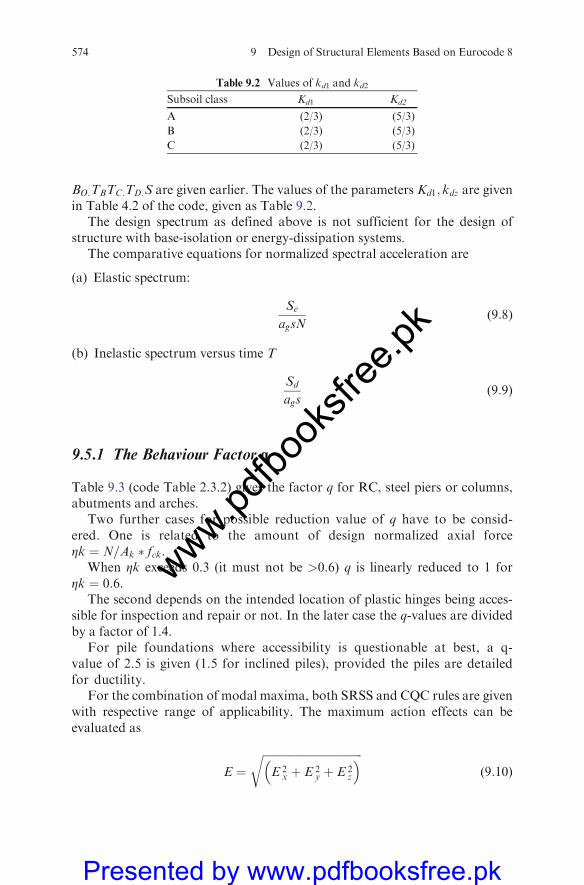
BO:TBTC:TD:S are given earlier. The values of the parameters Kd1; kdz are givenin Table 4.2 of the code, given as Table 9.2.
The design spectrum as defined above is not sufficient for the design ofstructure with base-isolation or energy-dissipation systems.
The comparative equations for normalized spectral acceleration are
(a) Elastic spectrum:
Se
agsN(9:8)
(b) Inelastic spectrum versus time T
Sd
ags(9:9)
9.5.1 The Behaviour Factor q
Table 9.3 (code Table 2.3.2) gives the factor q for RC, steel piers or columns,abutments and arches.
Two further cases for possible reduction value of q have to be consid-ered. One is related to the amount of design normalized axial forceZk ¼ N=Ak � fck.
When Zk exceeds 0.3 (it must not be >0.6) q is linearly reduced to 1 forZk ¼ 0:6.
The second depends on the intended location of plastic hinges being acces-sible for inspection and repair or not. In the later case the q-values are dividedby a factor of 1.4.
For pile foundations where accessibility is questionable at best, a q-value of 2.5 is given (1.5 for inclined piles), provided the piles are detailedfor ductility.
For the combination of modal maxima, both SRSS and CQC rules are givenwith respective range of applicability. The maximum action effects can beevaluated as
E ¼ffiffiffiffiffiffiffiffiffiffiffiffiffiffiffiffiffiffiffiffiffiffiffiffiffiffiffiffiffiffiffiffiffiffiffiffiE 2
x þ E 2y þ E 2
z
� �r(9:10)
Table 9.2 Values of kd1 and kd2
Subsoil class Kd1 Kd2
A (2/3) (5/3)
B (2/3) (5/3)
C (2/3) (5/3)
574 9 Design of Structural Elements Based on Eurocode 8
www.pdfbo
oksfr
ee.pk
Presented by www.pdfbooksfree.pk
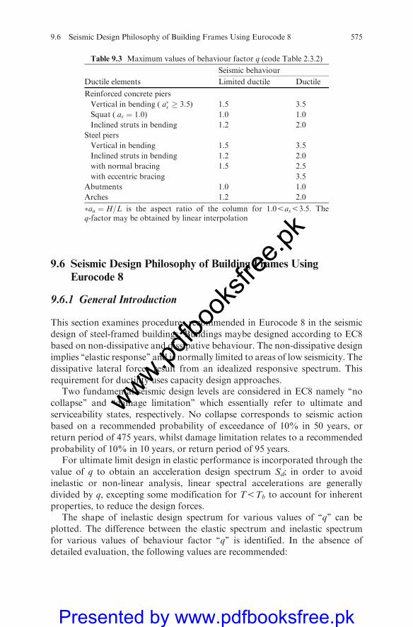
9.6 Seismic Design Philosophy of Building Frames Using
Eurocode 8
9.6.1 General Introduction
This section examines procedures recommended in Eurocode 8 in the seismic
design of steel-framed buildings. Buildings maybe designed according to EC8
based on non-dissipative and dissipative behaviour. The non-dissipative design
implies ‘‘elastic response’’ and is normally limited to areas of low seismicity. The
dissipative lateral forces result from an idealized responsive spectrum. This
requirement for ductility uses capacity design approaches.Two fundamental seismic design levels are considered in EC8 namely ‘‘no
collapse’’ and ‘‘damage limitation’’ which essentially refer to ultimate and
serviceability states, respectively. No collapse corresponds to seismic action
based on a recommended probability of exceedance of 10% in 50 years, or
return period of 475 years, whilst damage limitation relates to a recommended
probability of 10% in 10 years, or return period of 95 years.For ultimate limit design in elastic performance is incorporated through the
value of q to obtain an acceleration design spectrum Sd; in order to avoid
inelastic or non-linear analysis, linear spectral accelerations are generally
divided by q, excepting some modification for T5Tb to account for inherent
properties, to reduce the design forces.The shape of inelastic design spectrum for various values of ‘‘q’’ can be
plotted. The difference between the elastic spectrum and inelastic spectrum
for various values of behaviour factor ‘‘q’’ is identified. In the absence of
detailed evaluation, the following values are recommended:
Table 9.3 Maximum values of behaviour factor q (code Table 2.3.2)
Seismic behaviour
Ductile elements Limited ductile Ductile
Reinforced concrete piers
Vertical in bending ( a�s � 3:5) 1.5 3.5
Squat ( as ¼ 1:0) 1.0 1.0
Inclined struts in bending 1.2 2.0
Steel piers
Vertical in bending 1.5 3.5
Inclined struts in bending 1.2 2.0
with normal bracing 1.5 2.5
with eccentric bracing 3.5
Abutments 1.0 1.0
Arches 1.2 2.0
�aa ¼ H=L is the aspect ratio of the column for 1:05as53:5. Theq-factor may be obtained by linear interpolation
9.6 Seismic Design Philosophy of Building Frames Using Eurocode 8 575
www.pdfbo
oksfr
ee.pk
Presented by www.pdfbooksfree.pk
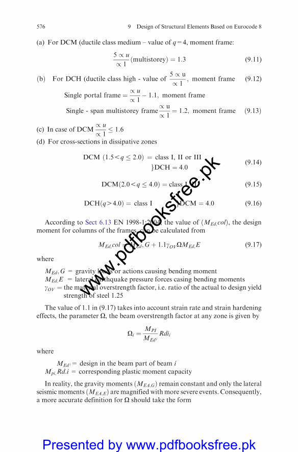
(a) For DCM (ductile class medium – value of q=4, moment frame:
5 / u
/ 1ðmultistoreyÞ ¼ 1:3 (9:11)
ðbÞ For DCH (ductile class high - value of5 / u
/ 1; moment frame (9:12)
Single portal frame ¼ / u
/ 1� 1:1; moment frame
Single - span multistorey frame/ u
/ 1¼ 1:2; moment frame ð9:13Þ
(c) In case of DCM/ u
/ 1� 1:6
(d) For cross-sections in dissipative zones
DCM 1:55q � 2:0ð Þ ¼ class I, II or III
gDCH ¼ 4:0(9:14)
DCMð2:05q � 4:0Þ ¼ class I. II (9:15)
DCHðq44:0Þ ¼ class I gDCM ¼ 4:0 (9:16)
According to Sect 6.13 EN 1998-1:2004, the value of ðMEd;colÞ, the designmoment for columns of the frames, can be calculated from
MEd;col ¼MEd;Gþ 1:1gOVOMEd;E (9:17)
where
MEd;G = gravity loads or actions causing bending momentMEd;E = lateral earthquake pressure forces casing bending momentsgOV ¼ the material overstrength factor, i.e. ratio of the actual to design yield
strength of steel 1.25
The value of 1.1 in (9.17) takes into account strain rate and strain hardeningeffects, the parameter O, the beam overstrength factor at any zone is given by
Oi ¼MPI
MEd i
Rdii
where
MEd i= design in the beam part of beam iMpi;Rd:i = corresponding plastic moment capacity
In reality, the gravity moments ðMEA;GÞ remain constant and only the lateralseismic moments ðMEA;EÞ aremagnified withmore severe events. Consequently,a more accurate definition for O should take the form
576 9 Design of Structural Elements Based on Eurocode 8
www.pdfbo
oksfr
ee.pk
Presented by www.pdfbooksfree.pk
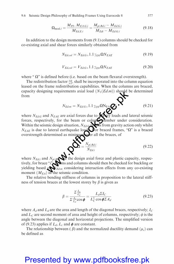
Omod:i ¼MPI�MEA:G:i
MEd;E:i¼Mpi:Rd:i �MEd:G:i
MEdi �MEd:G:i(9:18)
In addition to the design moments from (9.1) columns should be checked forco-existing axial and shear forces similarly obtained from
NEd:col ¼ NEd:Gþ1:1 gOVONEAE (9:19)
VEd;col ¼ VEd:Gþ1:1 gOVONEAE (9:20)
where ‘‘ O’’ is defined before (i.e. based on the beam flexural overstrength).The redistribution factor /u/1, shall be incorporated into the column equation
leased on the frame redistribution capabilities. When the columns are braced,capacity designing requirements axial load ðN1ðEd:mÞÞ should be determinedfrom
NEd:m ¼ NEd:Gþ1:1 gOVONEAE (9:21)
where NEd:G and NEAE are axial forces due to gravity loads and lateral seismicforces, respectively, for the beam or column member under consideration.Within the seismic design situation,NEd:G results from gravity action only whilstNEAE is due to lateral earthquake loads. For braced frames, ‘‘O’’ is a bracedoverstrength determined as minimum over all the braces, of
O ¼ Npi:Rd:i
NEd:i(9:22)
where NEd:i and Npi:Rd:i are the design axial force and plastic capacity, respec-tively, for brace ‘‘i’’. Beams and columns should then be checked for buckling oryielding based on NEd:m considering interaction effects from any co-existingmoment ðMEAÞ in the seismic condition.
The relative bending stiffness of columns in proposition to the lateral stiff-ness of tension braces at the lowest storey by b is given as
b ¼S Lc
L3C
S Ad
Ldcos f
¼ LdSICL3C cos fSAd
(9:23)
where Ad and Ld are the area and length of the diagonal braces, respectively; ICand LC are second moment of area and height of columns, respectively; f is theangle between the diagonal and horizontal projections. The simplified versionof (9.23) applies if Ld;Lc and f are constant.
The relationship between ( b) and the normalized ductility demand ðmrÞ canbe defined as
9.6 Seismic Design Philosophy of Building Frames Using Eurocode 8 577
www.pdfbo
oksfr
ee.pk
Presented by www.pdfbooksfree.pk
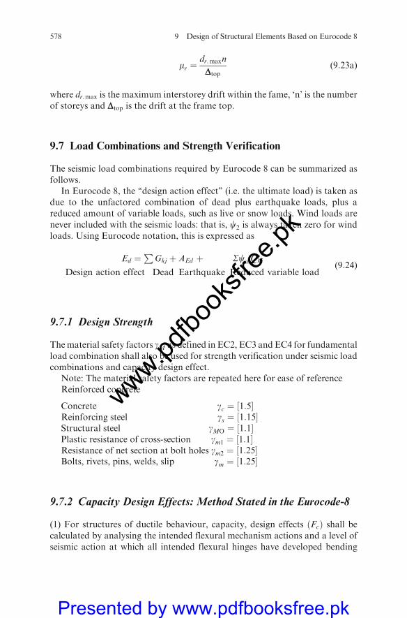
mr ¼dr:maxn
Dtop(9:23a)
where dr:max is the maximum interstorey drift within the fame, ‘n’ is the numberof storeys and Dtop is the drift at the frame top.
9.7 Load Combinations and Strength Verification
The seismic load combinations required by Eurocode 8 can be summarized asfollows.
In Eurocode 8, the ‘‘design action effect’’ (i.e. the ultimate load) is taken asdue to the unfactored combination of dead plus earthquake loads, plus areduced amount of variable loads, such as live or snow loads. Wind loads arenever included with the seismic loads: that is, c2 is always taken zero for windloads. Using Eurocode notation, this is expressed as
Ed ¼P
Gkj þ AEd þ ScaiQki
Design action effect Dead Earthquake Reduced variable load(9:24)
9.7.1 Design Strength
Thematerial safety factors gM as defined in EC2, EC3 and EC4 for fundamentalload combination shall also be used for strength verification under seismic loadcombinations and capacity design effect.
Note: The material safety factors are repeated here for ease of referenceReinforced concrete
Concrete gc ¼ ½1:5�Reinforcing steel gs ¼ ½1:15�Structural steel gMO ¼ ½1:1�Plastic resistance of cross-section gm1 ¼ ½1:1�Resistance of net section at bolt holes gm2 ¼ ½1:25�Bolts, rivets, pins, welds, slip gm ¼ ½1:25�
9.7.2 Capacity Design Effects: Method Stated in the Eurocode-8
(1) For structures of ductile behaviour, capacity, design effects ðFcÞ shall becalculated by analysing the intended flexural mechanism actions and a level ofseismic action at which all intended flexural hinges have developed bending
578 9 Design of Structural Elements Based on Eurocode 8
www.pdfbo
oksfr
ee.pk
Presented by www.pdfbooksfree.pk

moment equal to an appropriate upper fractile of their flexural resistance, called
moment overstrength MO.(2) The moment overstrength of section shall be calculated as
MO ¼ gO þMRd (9:25)
where
go is the value overstrength factorMRd is the design flexural strength of the section, in the selected direction and
sense, based on the actual section geometry and reinforcement configura-tion ( gm values for fundamental load combinations). In demandingMRd,the interaction with the axial force and eventually with the bendingmoment in the other direction, both resulting from the combination ofpermanent actions (gravity loads and prestressing) and the design seismicaction in the same direction and sense, shall be considered.
(3) P The value of the overstrength factor shall be taken in general as
go ¼ 0:7þ 0:2q (9:26)
where q is the relevant behaviour factor.In the case of reinforced concrete sections, with special confining rein-
forcement according to clause 6.2.1 of the code in which the value of the
normalized axial force
Zk ¼NEd
AC:fck(9:27)
exceeds 0.1,the value of overstrength factor shall be increased to
go ¼ 1þ 2ðZk � 0:1Þ2h i
ð0:7þ 0:2qÞ (9:28)
whereNEd is the value of the axial force at the plastic hinge corresponding to the
design seismic combination, which is positive if compressive
AC is the area of section andfck is the characteristic concrete strength.
(4) Within members containing plastic hinge(s), the capacity design bending
moment, MC, at the vicinity of the hinge shall not be assumed greater than the
relevant design flexural resistanceMRd of the hinge assesses according to clause
5.6.3.1.
9.7 Load Combinations and Strength Verification 579
www.pdfbo
oksfr
ee.pk
Presented by www.pdfbooksfree.pk
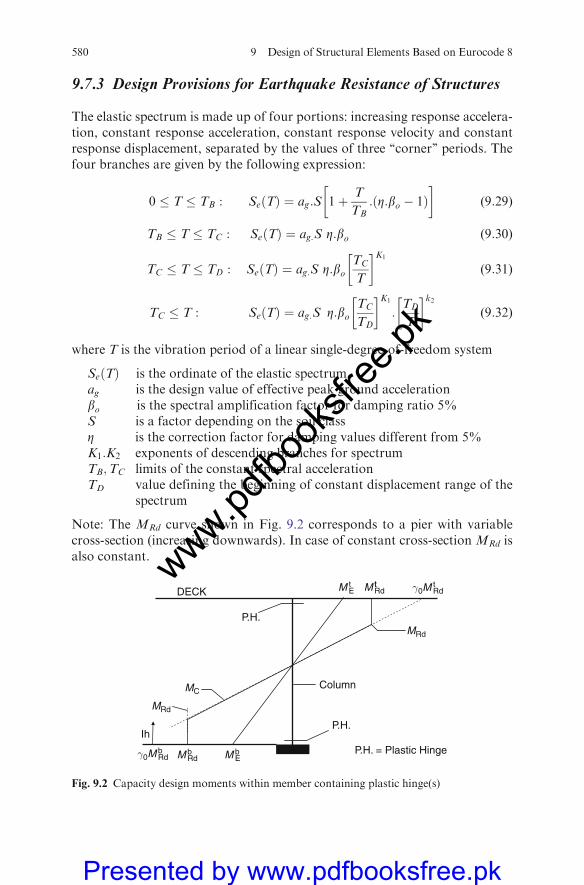
9.7.3 Design Provisions for Earthquake Resistance of Structures
The elastic spectrum is made up of four portions: increasing response accelera-tion, constant response acceleration, constant response velocity and constantresponse displacement, separated by the values of three ‘‘corner’’ periods. Thefour branches are given by the following expression:
0 � T � TB : Se Tð Þ ¼ ag:S 1þ T
TB: Z:bo � 1ð Þ
� �(9:29)
TB � T � TC : SeðTÞ ¼ ag:S Z:bo (9:30)
TC � T � TD : SeðTÞ ¼ ag:S Z:boTC
T
� �K1
(9:31)
TC � T : SeðTÞ ¼ ag:S Z:boTC
TD
� �K1
:TD
T
� �k2(9:32)
where T is the vibration period of a linear single-degree-of-freedom system
SeðTÞ is the ordinate of the elastic spectrumag is the design value of effective peak ground accelerationbo is the spectral amplification factor for damping ratio 5%S is a factor depending on the soil classZ is the correction factor for damping values different from 5%K1:K2 exponents of descending branches for spectrumTB;TC limits of the constant spectral accelerationTD value defining the beginning of constant displacement range of the
spectrum
Note: The MRd curve shown in Fig. 9.2 corresponds to a pier with variablecross-section (increasing downwards). In case of constant cross-section MRd isalso constant.
P.H.
P.H.
Column
DECK
P.H. = Plastic Hinge
Ih
M tE
M bEγ0M b
Rd M bRd
M ttRd γ0M t
Rd
MRd
MC
MRd
Fig. 9.2 Capacity design moments within member containing plastic hinge(s)
580 9 Design of Structural Elements Based on Eurocode 8
www.pdfbo
oksfr
ee.pk
Presented by www.pdfbooksfree.pk

(5) Capacity design effects shall be calculated in general for each sense of theseismic action in both the longitudinal and transverse directions. A relevantprocedure and simplifications are given in Annex G.
9.7.4 Second-Order Effects
In case of linear analysis, second-order effects may be estimated usingdisplacement:
dE ¼ 0:5ð1þ qÞdEe (9:33)
where q is the behaviour factor and dEe are the seismic displacement obtainedfrom the first-order elastic analysis.
9.7.5 Resistance Verification of Concrete Sections
(a) Design effects
(1) When the resistance of a section depends significantly on the interactionof more than one action effects (e.g. bendingmoments and axial force) itis sufficient that the ultimate limit state conditions, given in the respec-tive clauses, are satisfied separately by the extreme (max ormin) value ofeach action, taking into account the interaction with the coincidentalaccompanying values of the other actions.
(b) Structure of limit ductile behaviour
(1) PEd � Rd (9:34)
whereEd is the design action effect under the seismic load combination
including second-order effects andRd is the design resistance of the section.
(2) (P) In regions of moderate to high seismicity ða1g � ½0:10 g�Þ the shearresistance of potential plastic hinges shall be verified according to 5.6.3.4.
(c) Structures of ductile behaviourFlexural resistance of sections of plastic hinges
(1)MEd �MRd (9:34a)
whereMEd is the design moment under the seismic load combination,
including second-order effects and
9.7 Load Combinations and Strength Verification 581
www.pdfbo
oksfr
ee.pk
Presented by www.pdfbooksfree.pk

MRd is the design flexural resistance of the section, taking intoaccount the interaction of the accompanying design effects(axial force and eventually the bending moment in the otherdirection).
(2) P The longitudinal reinforcement of the member containing the hingeshall remain constant and fully active at least over the length lh indicatedin Fig. 9.2.
(d) Flexural resistance outside the region of plastic hinges
(1) MC �MRd (9:35)
whereMC is the capacity design moment as defined in Clause 5.3 andMRd is the design resistance of the section, taking into account the
interaction of the corresponding design effects (axial force andeventually the bending moment in the other direction).
(e) Shear resistance of elements outside the region of plastic hinges
(1) Verification of web diagonal compression
VC � VRdz (9:36)
(2) Verification of shear reinforcement
VC � VCd þ Vwd (9:37)
where VC is the shear force resulting from capacity design as per Clause 5.3.Design shear resistance shall be calculated according to EC2 part 1
VRdz
VCd ¼ VRdl
Vwd
Note: Formulae are repeated here, in concise form, to facilitate cross-reference
VRdz ¼ 0:5vfcdbw0:9d with v ¼ 0:7� fck
200� 0:5 (9:38)
Vcd ¼ VRd1 ¼ ½tRdkð1:2� 40r1Þ þ 0:15scp�bwd (9:39)
where
tRd ¼ 0:035fck
23
k ¼ 1:6� d � 1
582 9 Design of Structural Elements Based on Eurocode 8
www.pdfbo
oksfr
ee.pk
Presented by www.pdfbooksfree.pk

r1 ¼ Asl
bwd
� �40:02 is the ratio of longitudinal tension reinforcement
scp ¼ NEd
Acis the average normal stress under the design seismic effects,and d is the depth of the section in metres
Vwd ¼Asw
s
� �0:9dfywd (9:39a)
whereAsw and s are the area and spacing of the stirrups, respectively,fywd is the design yield strength of the shear reinforcement andbw is the width of the web of the section.
(e) Shear resistance of plastic hinges
(1) Verification of diagonal compression
VC5VRde (9:40)
whereVRde is the shear resistance corresponding to the compressive con-
crete strength after degradation
¼ 0:275vfckbwcdc (9:40a)
where
u ¼ 0:7� fck=200 � 0:5 and (9:41)
bmc and dc are confined web width and depth of the section, respectively.(2) Verification of shear reinforcement
Vc � Vcde þ Vwd (9:42)
where Vcde is the contribution of the concrete after degradation and is equal to
Vcde0 if Zk � 0:1 ðaÞVcde ¼ 2:5tRdbwcdc for Zk401 ðbÞwith Zk ¼ NEd
AccfckðcÞ
(9:43)
Vwd is the contribution of reinforcement calculated according to5.6.33 (2) of the code
NC is the design axial force and is positive if compressive and
9.7 Load Combinations and Strength Verification 583
www.pdfbo
oksfr
ee.pk
Presented by www.pdfbooksfree.pk
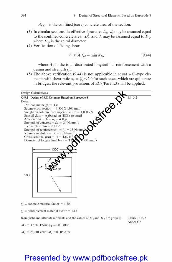
ACC is the confined (core) concrete area of the section.
(3) In circular sections the effective shear area bwc; dc may be assumed equalto the confined concrete area pD
24sp and dc may be assumed equal to Dsp
where Dsp is the spiral diameter.(4) Verification of sliding shear
Vc � Avfyd þminNEd (9:44)
where AV is the total distributed longitudinal reinforcement with adesign and strength fyd.
(5) The above verification (9.44) is not applicable in squat wall-type ele-ments with shear ratio as ¼ M
Vd52:0 for such cases, which are quite rare
in bridges; the relevant provisions of EC8/Part 1.3 shall be applied.
Design Calculations
Q.9.1 Design of RC Columns Based on Eurocode 8
Data:H= column height= 4 mSquare cross-section = 1,300 X1,300 (mm)Weight on column from superstructure = 4,000 kNSubsoil class= A (based on (EC8) assumedAcceleration = €U ¼ ag ¼ 400 galStrength of concrete ¼ fck ¼ 24 N=mm2;concrete strain = 0.0035
Strength of reinforcement ¼ fyk ¼ 35 N=mm2
Young’s modulus = Ec ¼ 25 N=mm2
Cross-sectional area = A = 1.69 m2
Diameter of longitudinal bars = T25 (AS = 491 mm2)
1300
2 Layers10T25–100
1300
gc ¼ concrete material factor = 1.50
gc ¼ reinforcement material factor = 1.15
from yield and ultimate moments and the values of Mu and MY are given as
MY = 17,880 kNm; fY ¼0.00140/m
Mu = 23,210 kNm: Mu =0.00556/m
1.1–3.2
Clause EC8/2
Annex C2
584 9 Design of Structural Elements Based on Eurocode 8
www.pdfbo
oksfr
ee.pk
Presented by www.pdfbooksfree.pk
Iun ¼ 1:3�1:3212¼ 0:2380m4
Icr ¼ MyðEcfyÞ ¼
17;88025 �ð106�0:0014Þ
�1¼0:510m4
T = fundamental period: Ieff ¼ 0:08� Iun þ Icr ¼ 0:529m4
K for column=3 EcIeffH2 ¼ 3�25�106�0:529
43= 619,922 (kN/m)
M ¼Wu þ 0:5Wp ¼ 4; 000þ 0:5ð4� 1:69� 25Þ¼ 4; 000þ 84:4 ¼ 4; 084:4
T ¼ffiffiffiffiffiffiffiM=gK
2pq
ffiffiffiffiffiffiffiffiffiffiffiffiffiffiffiffiffi4084:4=9:81
619922
2pq
¼ 0:1629 � 0:163
Design spectrum analysis with soil condition A
0 � T � TB SeðTÞ ¼ ag:s 1þ TTBðZb0 � 1Þ
h i
Design Calculations
ag ¼ 400� 1:3 ¼ 520 gal; a ¼ agG¼ 520
980¼ 0:531
S ¼ 1:0; b0 ¼ 2:5 Kdt ¼ 23
Table 4.1, q is fixed as 3.5 for height = 4.0 m and the length is 1.3, so
413� 3:077 � 3:50
TB ¼ 0:40 s;T ¼ 0:163 s
SeðTÞ ¼ 0:691540:20� 0:106
SeðTÞis fixed as 0.69
Verification of flexural resistance at the base of the column (the plastic hingeregion)
MA = the applied moment at the base of the column
¼ 4; 000� 4ð4�1:69�25Þ42gð0:69Þ ¼ 11; 273 kNm
n
The maximum elastic displacement at the top of the column
dEelastic ¼ 0:5 ð1þ qÞ dEe ¼ 0:5 1þ 3:6ð Þ � 0:018 ¼ 0:0414m
Dm, the additional moment (second-order effect)
4; 000 dE ¼ 4; 000� 0:0414 ¼ 165:6 kNmMAT ¼ the total applied moment = MA þ DM ¼ 16; 413:6KNM
EC B/2 -4.1.6
EC 8/2-4.2.1.4
9.7 Load Combinations and Strength Verification 585
www.pdfbo
oksfr
ee.pk
Presented by www.pdfbooksfree.pk
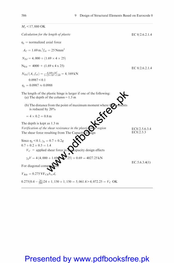
My517; 880 OK
Calculation for the length of plastic
Zk ¼ normalized axial force
AC ¼ 1:69m;2fck ¼ 25Nmm2
NEd ¼ 4; 000þ ð1:69� 4� 25Þ
NEd = 4000 + (1.69 x 4 x 25)
NEd=ðAc:fckÞ ¼ 4:169�1031�25�103�1:69 ¼ 4; 169 kN
0:098750:1
Zk ¼ 0:0987 � 0:0988
The length of the plastic hinge is larger if one of the following:(a) The depth of the column=1.3 m
(b) The distance from the point of maximummoment where themomentsis reduced by 20%
¼ 4� 0:2 ¼ 0:8m
The depth is kept as 1.3 m
Verification of the shear resistance in the plastic hinge region
The shear force resulting from The Capacity Design
Since Zk50:1; g0 ¼ 0:7þ 0:2q
0:7þ 0:2� 0:5 ¼ 1:4
VC = applied shear force in the capacity design effects
g0V ¼ 4 ð4; 000þ 1:69� 4� 25Þ � 0:69 ¼ 4027:25 kN
For diagonal compression
VRde ¼ 0:275VFCKbwcdc
0:275ð0:4� 24200Þ24� 1; 150� 1; 150 ¼ 5; 061:444; 072:25 ¼ VC OK
EC 8/2.6.2.1.4
EC 8/2.6.2.1.4
EC8/2.5.6.3.4EC8/2.5.3
EC.5.6.3.4(1)
586 9 Design of Structural Elements Based on Eurocode 8
www.pdfbo
oksfr
ee.pk
Presented by www.pdfbooksfree.pk
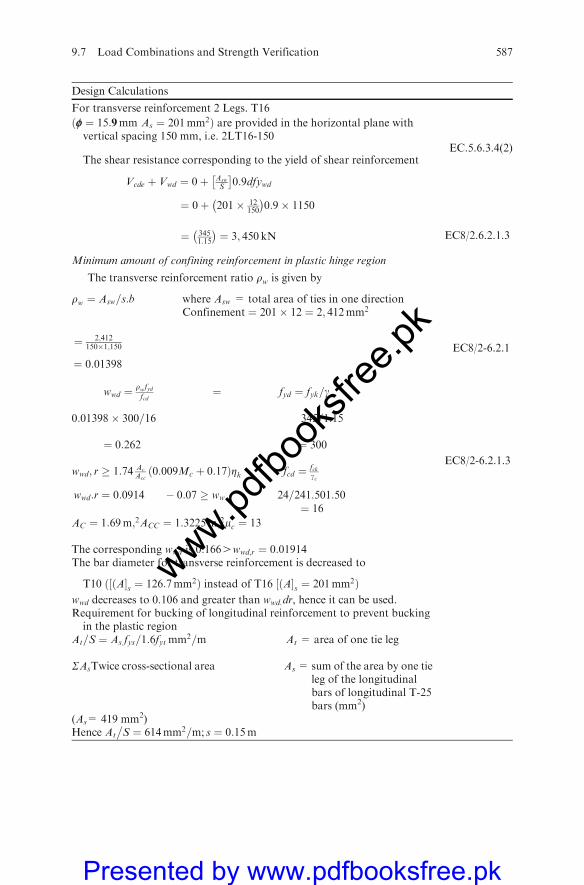
Design Calculations
For transverse reinforcement 2 Legs. T16
ðf ¼ 15:9mm As ¼ 201mm2Þ are provided in the horizontal plane withvertical spacing 150 mm, i.e. 2LT16-150
The shear resistance corresponding to the yield of shear reinforcement
Vcde þ Vwd ¼ 0þ Asw
S
0:9dfywd
¼ 0þ 201� 12150
� �0:9� 1150
¼ 3451:15
� �¼ 3; 450 kN
Minimum amount of confining reinforcement in plastic hinge region
The transverse reinforcement ratio rw is given by
rw ¼ Asw=s:b where Asw = total area of ties in one directionConfinement ¼ 201� 12 ¼ 2; 412mm2
¼ 2;412150�1;150
¼ 0:01398
wwd ¼ rwfydfcd
¼ fyd ¼ fyk=g
0:01398� 300=16 345=1:15
¼ 0:262 ¼ 300
wwd; r � 1:74 Ac
Accð0:009Mc þ 0:17ÞZk fcd ¼ fck
gc
wwd:r ¼ 0:0914 � 0:07 � ww 24 241:50= 1:50¼ 16
AC ¼ 1:69m;2ACC ¼ 1:3225m;2mc ¼ 13
The corresponding wwd is 0:1664wwd;r ¼ 0:01914The bar diameter for transverse reinforcement is decreased to
T10 ð½ðA�s ¼ 126:7mm2Þ instead of T16 ½ðA�s ¼ 201mm2Þwwd decreases to 0.106 and greater than wwd:dr, hence it can be used.Requirement for bucking of longitudinal reinforcement to prevent buckingin the plastic region
At=S ¼ As fys=1:6fyt mm2=m At = area of one tie leg
SAsTwice cross-sectional area As = sum of the area by one tieleg of the longitudinalbars of longitudinal T-25bars (mm2)
(As= 419 mm2)Hence At S ¼ 614mm2=m; s ¼ 0:15m
EC.5.6.3.4(2)
EC8/2.6.2.1.3
EC8/2-6.2.1
EC8/2-6.2.1.3
9.7 Load Combinations and Strength Verification 587
www.pdfbo
oksfr
ee.pk
Presented by www.pdfbooksfree.pk
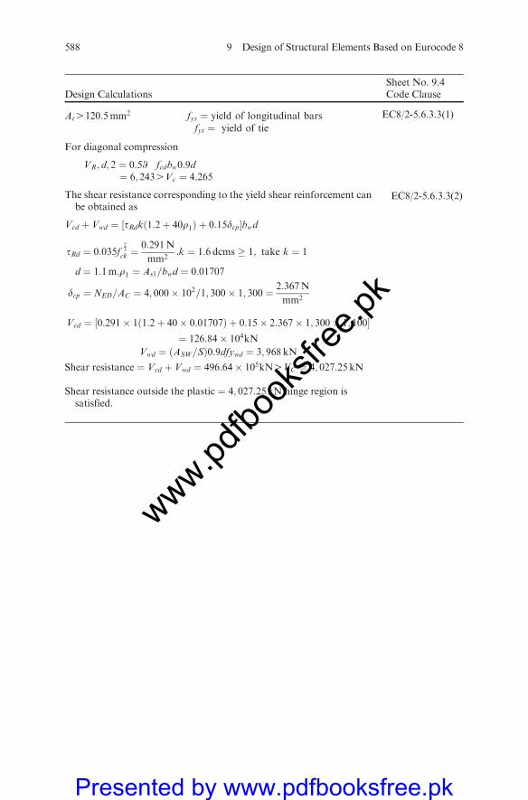
Design CalculationsSheet No. 9.4Code Clause
At4120:5mm2 fys ¼ yield of longitudinal barsfyt ¼ yield of tie
For diagonal compression
VR; d; 2 ¼ 0:5W fcdbw0:9d¼ 6; 2434Vc ¼ 4;265
The shear resistance corresponding to the yield shear reinforcement canbe obtained as
Vcd þ Vwd ¼ ½tRdkð1:2þ 40r1Þ þ 0:15dcp�bwd
tRd ¼ 0:035f23
ck ¼0:291N
mm2:k ¼ 1:6 dcms � 1; take k ¼ 1
d ¼ 1:1m;r1 ¼ As1=bwd ¼ 0:01707
dcp ¼ NED=AC ¼ 4; 000� 102=1; 300� 1; 300 ¼ 2:367N
mm2
Vcd ¼ ½0:291� 1ð1:2þ 40� 0:01707Þ þ 0:15� 2:367� 1; 300� 1; 100�¼ 126:84� 104kN
Vwd ¼ ðASW=SÞ0:9dfywd ¼ 3; 968 kN
Shear resistance ¼ Vcd þ Vwd ¼ 496:64� 105kN4VC ¼ 4; 027:25 kN
Shear resistance outside the plastic ¼ 4; 027:25 kN hinge region issatisfied.
EC8/2-5.6.3.3(1)
EC8/2-5.6.3.3(2)
588 9 Design of Structural Elements Based on Eurocode 8
www.pdfbo
oksfr
ee.pk
Presented by www.pdfbooksfree.pk
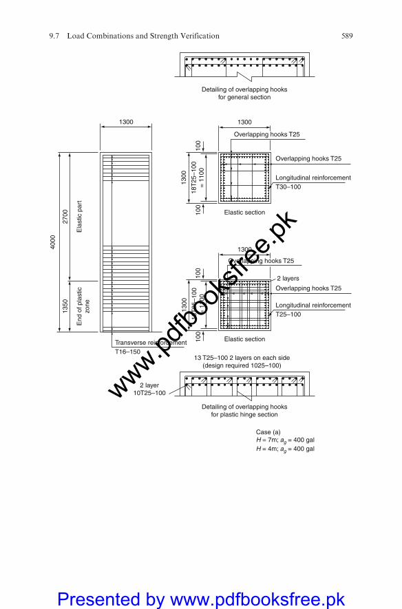
Elastic section
Detailing of overlapping hooksfor plastic hinge section
2 layer10T25–100
13 T25–100 2 layers on each side(design required 1025–100)
Case (a)H = 7m; ag = 400 gal
Elastic section
Detailing of overlapping hooksfor general section
Overlapping hooks T25
2 layers
Overlapping hooks T25
Overlapping hooks T25
Overlapping hooks T25
1300
100
100
100
100
1300
1300
1300
18T
25–1
00=
110
018
T25
–100
= 1
100
End
of p
last
iczo
neE
last
ic p
art
1350
4000
2700
1300
Longitudinal reinforcementT25–100
Longitudinal reinforcementT30–100
Transverse reinforcementT16–150
H = 4m; ag = 400 gal
9.7 Load Combinations and Strength Verification 589
www.pdfbo
oksfr
ee.pk
Presented by www.pdfbooksfree.pk
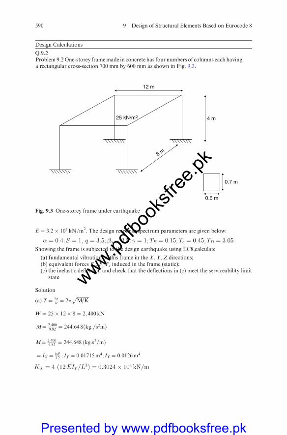
Design Calculations
Q.9.2Problem 9.2One-storey framemade in concrete has four numbers of columns each havinga rectangular cross-section 700 mm by 600 mm as shown in Fig. 9.3.
E ¼ 3:2� 107 kN=m2. The design response spectrum parameters are given below:
� ¼ 0:4;S ¼ 1; q ¼ 3:5;�o ¼ 2:5; � ¼ 1;TB ¼ 0:15;Tc ¼ 0:45;TD ¼ 3:05
Showing the frame is subjected to the design earthquake using EC8,calculate
(a) fundamental vibration of this frame in the X, Y, Z directions;(b) equivalent forces Fx, Fy,Fz induced in the frame (static);(c) the inelastic deflection and check that the deflections in (c) meet the serviceability limit
state
Solution
(a) T ¼ 2pw¼ 2p
ffiffiffiffiffiffiffiffiffiffiffiM K=
p
W ¼ 25� 12� 8 ¼ 2; 400 kN
M¼ 2;4009:82¼ 244:64 8ðkg: s2
mÞ
M¼ 2;4009:82 ¼ 244:648 ðkg:s2=mÞ
¼ IX ¼ bd3
12; IX ¼ 0:01715m4; IY ¼ 0:0126m4
KX ¼ 4 12EIY =L3ð Þ ¼ 0:3024� 104 kN=m
12 m
4 m
8 m
25 kN/m2
0.6 m
0.7 m
Fig. 9.3 One-storey frame under earthquake
590 9 Design of Structural Elements Based on Eurocode 8
www.pdfbo
oksfr
ee.pk
Presented by www.pdfbooksfree.pk

Design Calculations
Note:
L = 4 m
A ¼ 0:6� 0:7 ¼ 0:42m2 KY ¼ 4 12EIXL3
� �¼ 0:416� 106 kN=m
Kz ¼ 4EAH ¼ 4 32�106�0:42
4
h i¼ 13:44� 106 kN=m
TX ¼ 2pw¼
ffiffiffiffiffimKx
2pq
¼ 0:01787 s
Ty ¼ffiffiffiffimKy
2pq
¼ 0:1581 s
Tz ¼ffiffiffiffimKz
2pq
¼ 0:0268 s
(b) FX;FY;FZ
F ¼ ma
FX ¼MSdTxðiÞ a ¼ SdðtÞg
SdðTXÞ ¼ /Sboqg 0:150:178750:4
0:4�1�2:53:5 g ¼ 0:286:39 g
From
Fx ¼ 244:648� 0:286� 9:81 ¼ 686:39 kN
FY ¼ 656:399 kN
Fz ¼MSdðTzÞ � 0:7 g; Tz ¼ 0:026850:15 sreduction factor ¼ 0:7
0 � T � TB
0 � 0:268 � 0:1
Sdð0:268Þ ¼ as 1þ TTB
b0q� 1
� �h i
¼ 0:4 1þ 0:2680:1
2:53:5� 1� �
¼ 0:324
Fz ¼ 244:648� 0:3241� 0:7� 9:81 ¼ 544:409 kN
(c)dx:e ¼ Fx
Kx¼ 686:399
0:3024�106 ¼ 2:2675� 10�3 m
dx ¼ dxeðqÞ ¼ 7:936� 10�3 m
dr � h250
;dr ¼ 0:016
dx5dr7:936� 10�3m50:016m OK
Note: The individual column checking procedure as given in Example 9.1 shall be carriedout. This is not given in this solution owing to lack of space for repetitive work.
9.7 Load Combinations and Strength Verification 591
www.pdfbo
oksfr
ee.pk
Presented by www.pdfbooksfree.pk
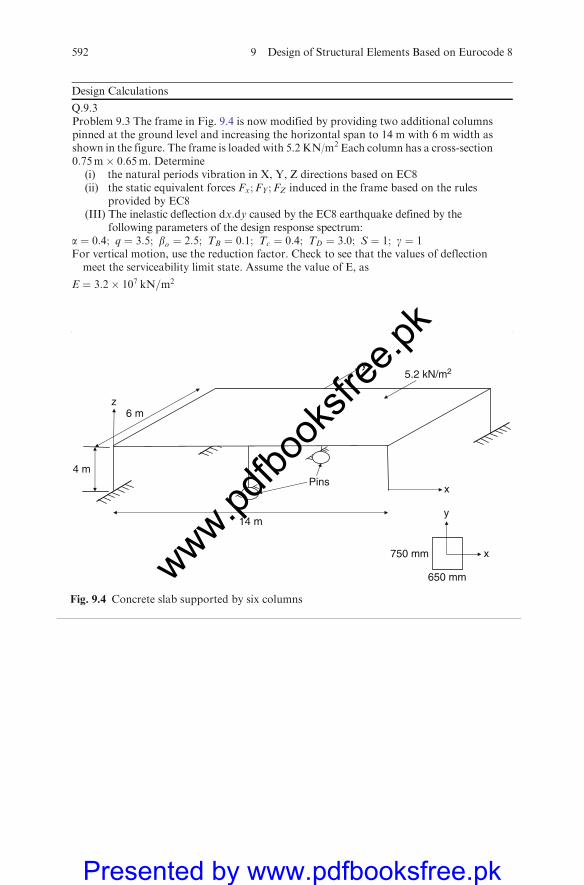
Design Calculations
Q.9.3Problem 9.3 The frame in Fig. 9.4 is now modified by providing two additional columnspinned at the ground level and increasing the horizontal span to 14 m with 6 m width asshown in the figure. The frame is loaded with 5.2 KN/m2 Each column has a cross-section0:75m� 0:65m. Determine
(i) the natural periods vibration in X, Y, Z directions based on EC8(ii) the static equivalent forces Fx;FY;FZ induced in the frame based on the rules
provided by EC8(III) The inelastic deflection dx:dy caused by the EC8 earthquake defined by the
following parameters of the design response spectrum:a ¼ 0:4; q ¼ 3:5; bo ¼ 2:5; TB ¼ 0:1; Tc ¼ 0:4; TD ¼ 3:0; S ¼ 1; g ¼ 1For vertical motion, use the reduction factor. Check to see that the values of deflectionmeet the serviceability limit state. Assume the value of E, as
E ¼ 3:2� 107 kN=m2
6 m
14 m
5.2 kN/m2
x
y
4 m
x
y
z
750 mm
650 mm
Pins
Fig. 9.4 Concrete slab supported by six columns
592 9 Design of Structural Elements Based on Eurocode 8
www.pdfbo
oksfr
ee.pk
Presented by www.pdfbooksfree.pk
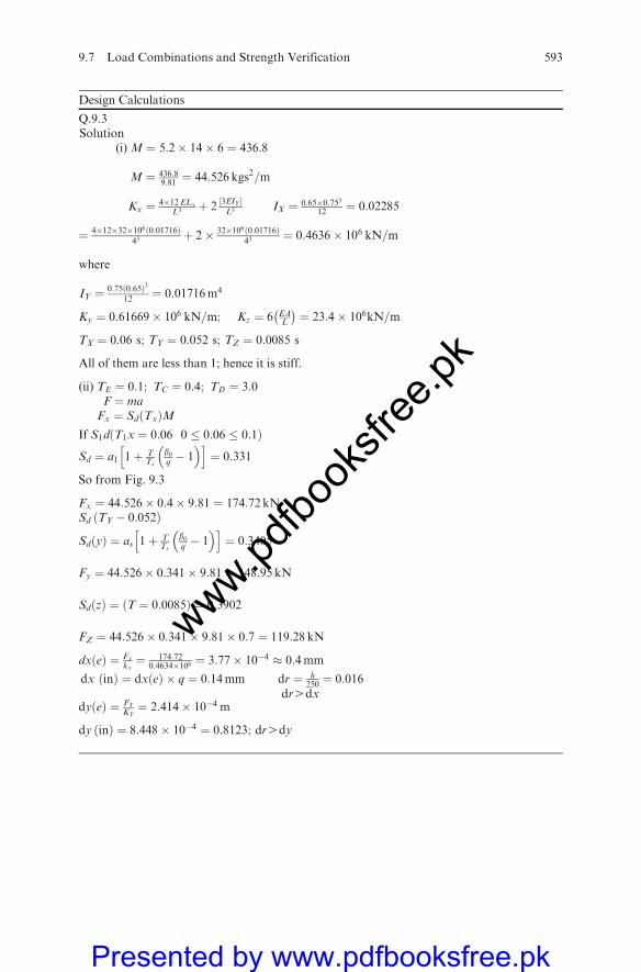
Design Calculations
Q.9.3Solution
(i) M ¼ 5:2� 14� 6 ¼ 436:8
M ¼ 436:89:81¼ 44:526 kgs2=m
Kx ¼ 4�12ELx
L3 þ 23EIY½ �L3 IX ¼ 0:65�0:753
12¼ 0:02285
¼ 4�12�32�106ð0:01716Þ43
þ 2� 32�106ð0:01716Þ43
¼ 0:4636� 106 kN=m
where
IY ¼ 0:75ð0:65Þ312
¼ 0:01716m4
Ky ¼ 0:61669� 106 kN=m; Kz ¼ 6 EAL
� �¼ 23:4� 106kN=m
TX ¼ 0:06 s; TY ¼ 0:052 s; TZ ¼ 0:0085 s
All of them are less than 1; hence it is stiff.
(ii) TE ¼ 0:1; TC ¼ 0:4; TD ¼ 3:0F ¼ ma
Fx ¼ SdðTxÞMIf S1dðT1x ¼ 0:06 0 � 0:06 � 0:1ÞSd ¼ a1 1þ T
Ts
b0q� 1
� �h i¼ 0:331
So from Fig. 9.3
Fx ¼ 44:526� 0:4� 9:81 ¼ 174:72 kNSd ðTY � 0:052Þ
SdðyÞ ¼ as 1þ TTs
b0q� 1
� �h i¼ 0:3405
Fy ¼ 44:526� 0:341� 9:81 ¼ 148:95 kN
SdðzÞ ¼ ðT ¼ 0:0085Þ ¼ 0:3902
FZ ¼ 44:526� 0:341� 9:81� 0:7 ¼ 119:28 kN
dxðeÞ ¼ Fx
kx¼ 174:72
0:4634�106 ¼ 3:77� 10�4 � 0:4mm
dx ðinÞ ¼ dxðeÞ � q ¼ 0:14mm dr ¼ h250¼ 0:016
dr4dxdyðeÞ ¼ FY
KY¼ 2:414� 10�4 m
dy ðinÞ ¼ 8:448� 10�4 ¼ 0:8123; dr4dy
9.7 Load Combinations and Strength Verification 593
www.pdfbo
oksfr
ee.pk
Presented by www.pdfbooksfree.pk
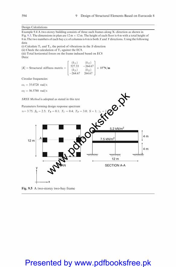
Design Calculations
Example 9.4 A two-storey building consists of three such frames along X- direction as shown inFig. 9.5. The dimensions in plan are 12m� 12m. The height of each floor is 4 m with a total height of8m.The two numbers of each bay c/c of columns is 6m is bothX andY directions. Using the followingdata(i) Calculate T1 and T2, the period of vibrations in the X-direction(ii) Check the calculation of T1 against the EC8.(iii) Total horizontal forces on the frame induced based on EC8Data:
½K� ¼ Structural stiffness matrix ¼
ðk11Þ ðk12Þ527:33 �264:67ðk21Þ ðk22Þ�264:67 264:67
2664
3775� 106N=m
Circular frequencies:
o1 ¼ 35:0728 rad=s
o2 ¼ 56:5788 rad=s
SRSS Method is adopted as stated in this text
Parameters forming design response spectrum
/¼ 3:75; b0 ¼ 2:5; TB ¼ 0:1; TC ¼ 0:4; TD ¼ 3:0; S ¼ 1; g1 ¼ 1
4 m
12 m 12 m
12 m
4 m
7.5 kN/m2A
5.2 kN/m2
AA
x
ySECTION A-APLAN
Fig. 9.5 A two-storey two-bay frame
594 9 Design of Structural Elements Based on Eurocode 8
www.pdfbo
oksfr
ee.pk
Presented by www.pdfbooksfree.pk
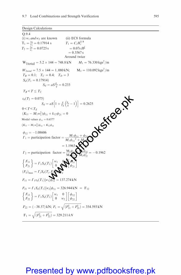
Design Calculations
Q:9:4ðiÞw1 andw2 are known (ii) EC8 formula
T1 ¼ 2pw1¼ 0:17914 s T1 ¼ CtH
3=4t
T2 ¼ 2pwz¼ 0:0725 s ¼ 0:07sH
34
¼ 0:3567 sAround twice
W1total ¼ 5:2� 144 ¼ 748:8 kN M1 ¼ 76:330 kgs2=m
W2total ¼ 7:5� 144 ¼ 1; 080 kN; M2 ¼ 110:092 kgs2=m
TB ¼ 0:1; TC ¼ 0:4; TD ¼ 3
SdðT1 ¼ 0:17914ÞSd ¼ aS bo
q¼ 0:233
TB5T � TC
sdðT2 ¼ 0:075ÞSd ¼ aS 1þ T
TB
boq� 1
� �h i¼ 0:2625
05T5TE
ðK11 �M1w21Þf11 þ k12f21 ¼ 0
Modal values f11 ¼ 0:6577
K11 �M1w22
� �f12 þ K12f21
f12 ¼ �1:08606G1 ¼ participation factor ¼ M1f11 þ f21
M1f112 þM2f21
2
¼ 1:1963
G2 ¼ participation factor ¼ M1f12 þM2f22
M1f212 þM2f
222
¼ � 0:1962
F11
F21
� �¼ G1SdðT1Þ
w1 00 w2
� �f11
f21
� �
ðFijÞmax ¼ GjSdðTj;EjÞ½w�fij
F11 ¼ G1sdðT1Þ½w1�f11 ¼ 137:274 kN
F21 ¼ G1SdðT1Þ½w2�f11 ¼ 326:944 kN ¼ F12
F12
F22
� �¼ G1SdðT1Þ
w1 00 w2
� �f12
f22
� �
F22 ¼ ð�38:57ÞkN; F1 ¼ffiffiffiffiffiffiffiffiffiffiffiffiffiffiffiffiffiffiffiffiffiffiffiðF2
11 þ F221Þ
q¼ 354:593 kN
F1 ¼ffiffiffiffiffiffiffiffiffiffiffiffiffiffiffiffiffiffiffiffiffiffiffiðF2
21 þ F222Þ
q¼ 329:211 kN
9.7 Load Combinations and Strength Verification 595
www.pdfbo
oksfr
ee.pk
Presented by www.pdfbooksfree.pk
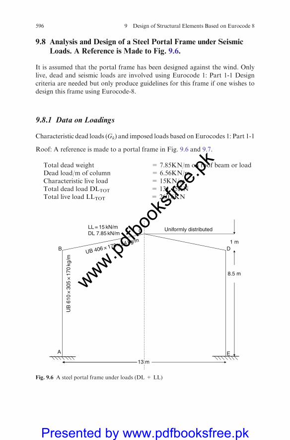
9.8 Analysis and Design of a Steel Portal Frame under Seismic
Loads. A Reference is Made to Fig. 9.6.
It is assumed that the portal frame has been designed against the wind. Only
live, dead and seismic loads are involved using Eurocode 1: Part 1-1 Design
criteria are needed but only produce guidelines for this frame if one wishes to
design this frame using Eurocode-8.
9.8.1 Data on Loadings
Characteristic dead loads (Gk) and imposed loads based on Eurocodes 1: Part 1-1
Roof: A reference is made to a portal frame in Fig. 9.6 and 9.7.
Total dead weight = 7.85KN/m on roof beam or loadDead load/m of column = 6.56KN/mCharacteristic live load = 15KN/mTotal dead load DLTOT = 131.45KNTotal live load LLTOT = 260.6KN
1 m
13 m
8.5 m
E
D
C
B
A
Uniformly distributedLL = 15 kN/m
UB
610
× 3
05 ×
170
kg/
m
UB 406 × 178 × 54 kg/mDL 7.85 kN/m
Fig. 9.6 A steel portal frame under loads (DL + LL)
596 9 Design of Structural Elements Based on Eurocode 8
www.pdfbo
oksfr
ee.pk
Presented by www.pdfbooksfree.pk
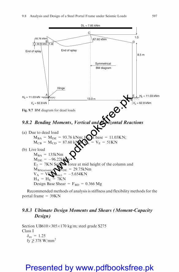
9.8.2 Bending Moments, Vertical and Horizontal Reactions
(a) Due to dead loadMBA = MDE = 93.76 kNm; HA at base = 11.03KN;MCB = MCD = 87.60 kNm VA = VE = 51KN
(b) Live loadMBA = 135kNmMDE = �96.22kNmE2 = 7KN Seismic force at mid height of the column andMBA(seismic) �MDE = 29.75kNmVA = VE(seismic) = �5.654KNHA = HE = 7KNDesign Base Shear = FBD = 0.366 Mg
Recommendedmethods of analysis is stiffness and flexibility methods for theportal frame = 39KN
9.8.3 Ultimate Design Moments and Shears (Moment-CapacityDesign)
Section UB610�305�170 kg/m; steel grade S275Class I
duv = 1.25fy � 378 W/mm2
1.0
13.0 m
8.5 m
E
D
C
B
A
Symmetrical
BM diagram
Hinge
HA = 11.03 kN
Va = 62.8 kN
1.0
93.76 kNm
82.73 kNm
HE = 11.03 kNm
87.60 kNm
1.8
End of splay
Ve = 62.8 kNm
End of splay
DL = 7.85 kNm
Fig. 9.7 BM diagram for dead loads
9.8 Analysis and Design of a Steel Portal Frame under Seismic Loads 597
www.pdfbo
oksfr
ee.pk
Presented by www.pdfbooksfree.pk

Max. ultimate design moment at YY axis = MED = 844kNmMax. ultimate shear = 95KNMax. Axial thrust = 194KN
Follow the eurocode EC-8 and Eurocode-3, check this frame for the seismic
combination of actions and prove that the frame is safe.
Guidelines for solution
1. Develop the BM diagram for live load and to account for the base force dueto seismic action.
2. Total load on the column of frame.3. Choose the analysis such as
(a) Flexibility method(b) Stiffness method(c) Handbook formulae (Kleinlogel Rahman Formula).
4. Assume member size given above and carry out solutions for momentsshear and axial effects using one of the abovemethod. Draw BMdiagram atcaves level due to the combination of seismic loads.
5. Check for seismic combination of actions for columns and pure in parts andbeams.
6. Classify the section, in this will come out to be class 1 while checking theflang and web.
7. Carry out moment capacity design using EC-5 and EC-8.8. Check the size UB610�305�170 kg/m; steel grade S = 275.9. Check for the dissipative zones expected to yield before other zones.
10. Check shear buckling resistance and buckling resistance to compression onall load combinations.
11. Check the plastic moment of resistance, plastic moment capacity, shear andbuckling effects such as for shear and
Conclusion. For columns UB 610�305�179 kg/m; S = 275 is ok.For beam UB 406�178�54 kg/m is ok.
598 9 Design of Structural Elements Based on Eurocode 8
www.pdfbo
oksfr
ee.pk
Presented by www.pdfbooksfree.pk
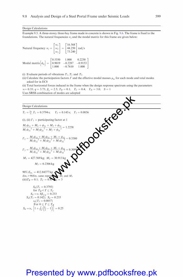
Design Calculations
Example 9.5. A three-storey three-bay frame made in concrete is shown in Fig. 9.6. The frame is fixed to the
foundations. The natural frequencies wj and the modal matrix for this frame are given below:
Natural frequency wj ¼w1
w2
w3
24
35 ¼
16:56844:25073:240
24
35 rad=s
Modal matrix fij
h i¼
0:5350 1:000 0:22300:9019 �0:2287 �0:91531:000 �0:7610 1:000
24
35
(i) Evaluate periods of vibrations T1;T2 and T2:
(ii) Calculate the participation factors G and the effective modal masses mm for each mode and total modes
asked for in EC8
(ii) Total horizontal forces induced in the frame when the design response spectrum using the parameters
/¼ 0:35; q ¼ 3:75; bo ¼ 2:5; TB ¼ 0:1; TC ¼ 0:4; TD ¼ 3:0; S ¼ 1
Uses SRSS combination of modes are adopted
Design Calculations
T1 ¼ 2pw ;
T1 ¼ 0:3794 s; T2 ¼ 0:143 s; T3 ¼ 0:0856
(i), (ii) G1 ¼ participating factor at 1
M1f11 þM2 þ f21 þM2 þ f31
M1f2
11 þM2f2
21 þM2 þ f 231
¼ 1:2258
G2 ¼ M1f12 þM2f22 þM3 þ f32
M1f 212 þM2f 2
22 þM3f 232
¼ 0:3380
G3 ¼ M1f12 þM2f23 þM3 þ f32
M1f2
12 þM2f2
22 þM3f2
32
¼ 0:3099
M1 ¼ 427:569 kg; M2 ¼ 30:913 kg
M3 ¼ 0:2306 kg
90%Em1¼ 412:84377 kg
Em1490Em1 same repeated for M2 and M3
(iii)TB ¼ 0:1; TC ¼ 0:4; TD ¼ 3
SdðT1 ¼ 0:3793Þfor TB5T � TC
Sd ¼/ Sbo=q ¼ 0:233SdðT2 ¼ 0:142Þ; Sd ¼ 0:233
sdðT3 ¼ 0:0857ÞFor 0 � T � TB
Sd ¼/s 1þ TTB
bo
q� 1
� �h i¼ 0:25
9.8 Analysis and Design of a Steel Portal Frame under Seismic Loads 599
www.pdfbo
oksfr
ee.pk
Presented by www.pdfbooksfree.pk

F11
F21
F32
8<:
9=; ¼ G1Sd1
w1 0 00 w2 00 0 w3
24
35 f11
f21
f31
8<:
9=;
F11 ¼ 305:30 kN! F1
F21 ¼ 386:5 kN! F21
F31 ¼ 385:590 kN! F31
M3 = 101.9367 (kg s2/m)
M2 = 152.9051
M1 = 203.8735
3
2
1
4m
4m
4m
Fig. 9.8 A three bay three-storey frame
600 9 Design of Structural Elements Based on Eurocode 8
www.pdfbo
oksfr
ee.pk
Presented by www.pdfbooksfree.pk
Chapter 10
Earthquake – Induced Collision, Pounding
and Pushover of Adjacent Buildings
10.1 General Introduction
The pounding of adjacent structures during earthquakes has been receivingconsiderable attention in recent years. This is because adjacent structures withinadequate clear spacing between them have suffered considerable structuraland non-structural damage as a result of their collision during major earth-quakes. The different dynamic characteristics of adjacent buildings make thenvibrate out of phase, and pounding occurs if there is a lack of sufficient spacebetween them. However, building code provisions for seismic separations inseismically active regions are not applicable, not only in the old parts of thecities but also in many cases in new buildings, due to socioeconomic implica-tions. Moreover, pounding between adjacent structures is a highly complexphenomenon, and its accurate modelling requires great details of informationof the structures in conjunction with a very reliable analytical method. Ingeneral, inelastic and plastic deformation, local crushing as well as impact-induced fracturing may occur at contacts during impact and pounding.
In this chapter the phenomenon of mutual interaction between neighbouringbuildings and the parameters that are affecting it are described thoroughly. Therequired separation distance between adjacent buildings in order to reducepounding is studied as well as the building code provisions for seismic separa-tions. Earthquake ground motion spatial variation effects on relative linearelastic response of adjacent buildings and their vibration characteristics areanalysed and also analytical solutions for the relative impact velocity arederived when adjacent buildings collide. Finally, the contact impact model istreated by the Lagrange multiplier method, which enforces compatibility ofdisplacements for the bodies coming into contact. Many other methods includ-ing the modal analysis given in Chap. 5 have also been recommended.
It has been observed, during powerful earthquakes, that in neighbouringbuildings, which are tangential to each other or have small separation distancebetween them so that they can collide with each other, their dynamic behaviouris mutually influenced in an important scale. In these conditions the phenomenathat are developed from the impact have as a result the mutual interaction ofthese buildings and also the drastic change of their dynamic response.
M.Y.H. Bangash, Earthquake Resistant Buildings,DOI 10.1007/978-3-540-93818-7_10, � M.Y.H. Bangash 2011
601
www.pdfbo
oksfr
ee.pk
Presented by www.pdfbooksfree.pk
During these phenomena, the presence of defects is possible, not only in thebuilding itself but also in the secondary elements of the mutually impactedbuildings. The defects of the building can be developed in positions that arecrucial for the behaviour of buildings, having as a possible result some or totalcollapse of the buildings.
This phenomenon is calledmutual interaction between neighbouring buildingsunder the conditions of seismic actions.
If the neighbouring buildings donot come in contactwith each other, because theseparation distance between them is big enough, but they are founded in soft soilsthen there is still the possibility of mutual interaction in their dynamic behaviour. Inthis case the mutual interaction is immediate, via the soil of the foundation.
For example, poundings between structures have been observed in the Alaskaearthquake of 1964, San Fernando earthquake of 1971, Mexico City earthquakeof 1985, Loma Prieta earthquake of 1989 in California, Kobe earthquake of 1995,TaiwanChi-Chi earthquake of 1999, the Sequenay earthquake of 1988 inCanada,the 1992 Erzincan earthquake in Turkey and the 1992Cairo earthquake. Recentlymany earthquakes occurred in Turkey, Iran andPakistan. The earthquake in 2006has destroyed Margalla Tower in Islamabad, Pakistan, and prior to collapse, theadjacent floors–walls interacted, eventually causing a total collapse.
The influence of the following factors when collision occurs between adja-cent buildings need to be examined in detail if possible:
1. The sizes of the building masses that impact or pound2. The stiffness and damping of each building3. The number of storeys of each building and in the height that the pounding
impact occurs4. The separation distance between the adjacent buildings must be such that
mutual pounding does not occur5. The surface of the impact6. The elastic–plastic behaviour of the buildings and their plasticity and crack-
ing levels7. The simulation on the foundation of the buildings8. The intensity and the dynamic characteristics of the
Apart from item 4, information does exist in each case mentioned in items1–3 and 5–8.
Initially, a simplified model of several adjacent buildings in a block was usedto study the pounding of such buildings due to strong earthquakes. Consider-able structural damage and even some collapses have sometimes been attributedto this effect. Each building is modelled as a SDOF system and pounding issimulated using impacted elements. A parametric investigation of this problemshows that the end structural elements almost always have substantial increasesin their response while for ‘‘interior’’ elements the opposite often happens. Thisexplains why high percentages of corner buildings have collapsed in manyearthquakes. Moreover, the effects of gap size, structural strength, relativemass size as well as impact element damping and stiffness need to be investigated.
602 10 Earthquake – Induced Pounding of Adjacent Buildings
www.pdfbo
oksfr
ee.pk
Presented by www.pdfbooksfree.pk
It is proposed to model pounding first between two adjacent buildings, withnatural periods T1 and T2 and damping z1 and z2 under harmonic earthquakeexcitation, as non-linear Hertzian impact between two SDOF systems. Analy-tical solution for the impact velocity can be derived for the case of rigid impacts.Inelastic impact will also be modelled by incorporating a coefficient of restitu-tion. For more general cases of non-rigid impacts, numerical simulations can becarried out to examine the applicability of the analytical solution for rigidimpacts and to investigate the maximum impact velocity.
An effective solution for studying the pounding response of adjacent build-ings during earthquakes can be carried out using the Lagrange multiplierapproach by which the geometric compatibility conditions due to contact areenforced. The energy and momentum balance criteria for contacting buildingsare satisfied according to the laws of impact covering post-impact conditions,which can also take into account local energy absorption phenomena duringcollision. A solution scheme is proposed which can be incorporated easily intoexisting computer programs for static and dynamic analysis of buildings asproposed in earlier chapters with and without seismic devices.
In many practical applications building structures are often constructed withnarrow gaps between adjacent but independent substructures. Examples includemechanical equipment within nuclear power plants, multi-span highway bridgesandmultistorey offices and parking structures.When responding to dynamic loads,the different dynamic characteristics of the individual units make them vibrate out-of-phase and mutual impact therefore occurs if the original gap size is too small.
In this chapter a simplifiedMDOF numerical model for analysis of the lateralcollision between adjacent buildings subjected to base excitation is suggestedalong with others. This model is based on the assumption that when the adjacentbuilding structural elements are collided with relatively high velocity and/or thelocal stiffness at the location of contact is much higher than global stiffness of theinvolved systems, then the duration of each collision can be assumed as zero, andthe change in potential energy of the system is negligible. As a result, theconstraints between the structural elements are removed and the original systemis replaced by pairs of colliding masses. The principle of conservation of momen-tum and the coefficient of restitution is applied to each floor independently touniquely determine the incremental velocities corresponding to each impact. Theproblem, therefore, turns to be a set of MDOF systems subjected to a series ofsudden change in velocities. BANG-Fhas a solution scheme described in the text.It is interesting to note the following papers by Chopra A. K and Goel R.K. Thereader must note these:
(a) A modal pushover analysis procedure for estimating seismic demands forbuildings. Earthquake Eng. Struct. Dyn. 2002; 31, 561–582.
(b) Amodal pushover analysis procedure to estimate seismic demands for unsym-metric-plan buildings. Earthquake Eng. Struct. Dyn. 2004; 33, 903–927.
Here some improved pushover analysis (MPA) procedure which retains(a) conceptual simplicity and computational attractiveness modal approach is
10.1 General Introduction 603
www.pdfbo
oksfr
ee.pk
Presented by www.pdfbooksfree.pk
adopted. In paper (b) a comprehensive MPA procedure with invariant forcedistribution is given for unsymmetrically planned building. Here again modalapproach is adopted. The reader is already familiar with the modal procedureearlier. Where seismic devices are employed, the right equation of motion inChopra A.K. et al. formulation be adopted, particularly for non-linear analysis.Where interation analysis can be carried out for pushover with non-equalheights of buildings, a reference is made to the following paper: C.G KaraYannis and Maria. J. Favvata, Earthquake induced interaction between adja-cent reinforced concrete structures with non-equal heights, Earthquake Engng.Struct. Dyn. 2005; 34, 1–20.
Here the authors developed a paper on the influence of structural poundingon the ductility requirement and the seismic behaviour of RC structuresdesigned according to EC2 and EC8 with non-equal heights.
10.2 Analytical Formulation for the Pushover
It is indeed very difficult to decide which method is to be used successfully toachieve the economic pushover results. The floors are modelled as adjacentmasses. If the buildings are of equal heights or of unequal heights, theequations of equilibrium can be established. Building with equal heightshaving adjacent masses can be treated as a contact impact case such thateach pair of masses vibrates initially along the line joining their centres.They should then collide head on while moving along the same straight lineafter collision. The collision is generally inelastic such that the local energyabsorption phenomenon during impact can be taken into account. The secondNewton’s law can be used for generalizing equations of equilibrium for anycase of building configurations. Again the buildings with and without seismicdevices can easily be devised using dynamic equations. Such equations arewith and without devices.
The generalized equilibrium equation for a pair of buildings can be written as
ma½ �t €uf gtaþ c½ �ta _uf gtaþ k½ �ta uf gta¼ � ma½ �t If g€xg � Ff gt�Building ‘‘a’’ (10:1)
mb½ �t €uf gtbþ c½ �tb _uf gtbþ k½ �tb uf gtb¼ � mb½ �t If g€xg � Ff gt�Building ‘‘b’’ (10:2)
such that one has to look for
uf ga� uf gb� d (10:3)
where uf g; _uf g and €uf g are the displacement, velocity and acceleration of eachbuilding such as buildings (a) and (b).
€xg= acceleration of supportIf g= influence coefficient column vector
604 10 Earthquake – Induced Pounding of Adjacent Buildings
www.pdfbo
oksfr
ee.pk
Presented by www.pdfbooksfree.pk
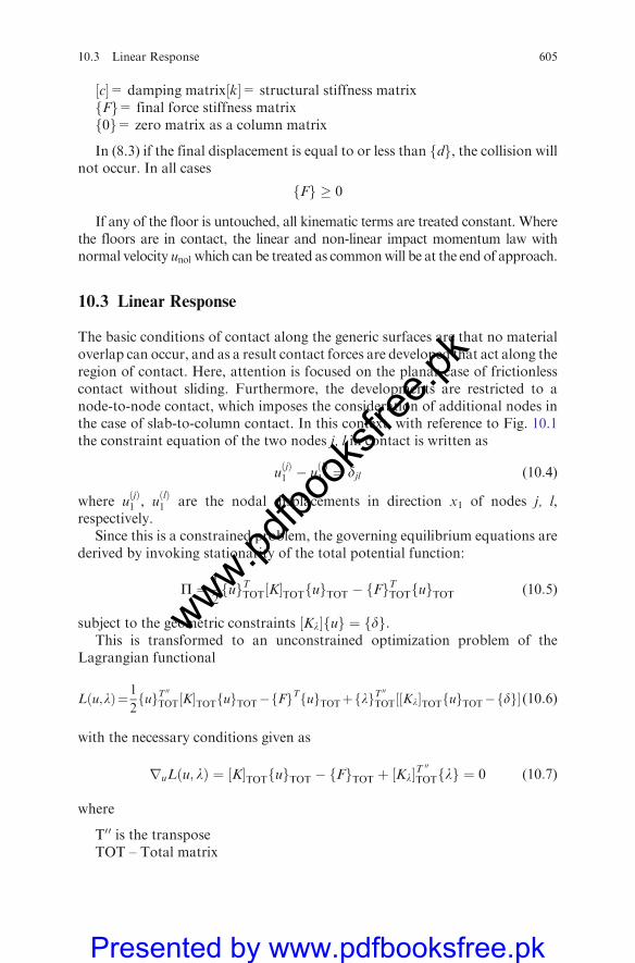
c½ �= damping matrix k½ �= structural stiffness matrixFf g= final force stiffness matrix0f g= zero matrix as a column matrix
In (8.3) if the final displacement is equal to or less than df g, the collision willnot occur. In all cases
Ff g � 0
If any of the floor is untouched, all kinematic terms are treated constant. Wherethe floors are in contact, the linear and non-linear impact momentum law withnormal velocity unol which can be treated as commonwill be at the end of approach.
10.3 Linear Response
The basic conditions of contact along the generic surfaces are that no materialoverlap can occur, and as a result contact forces are developed that act along theregion of contact. Here, attention is focused on the planar case of frictionlesscontact without sliding. Furthermore, the developments are restricted to anode-to-node contact, which imposes the consideration of additional nodes inthe case of slab-to-column contact. In this context, with reference to Fig. 10.1the constraint equation of the two nodes j, l in contact is written as
uðjÞ1 � u
ðlÞ1 ¼ djl (10:4)
where uðjÞ1 , u
ðlÞ1 are the nodal displacements in direction x1 of nodes j, l,
respectively.Since this is a constrained problem, the governing equilibrium equations are
derived by invoking stationarity of the total potential function:
P ¼ 1
2fugTTOT½K�TOTfugTOT � fFg
TTOTfugTOT (10:5)
subject to the geometric constraints ½Kl�fug ¼ fdg.This is transformed to an unconstrained optimization problem of the
Lagrangian functional
Lðu;lÞ¼1
2fugT
00
TOT½K�TOTfugTOT�fFgTfugTOTþflg
T 00
TOT½½Kl�TOTfugTOT�fdg� (10:6)
with the necessary conditions given as
ruLðu; lÞ ¼ ½K�TOTfugTOT � fFgTOT þ ½Kl�T00
TOTflg ¼ 0 (10:7)
where
T00 is the transposeTOT – Total matrix
10.3 Linear Response 605
www.pdfbo
oksfr
ee.pk
Presented by www.pdfbooksfree.pk
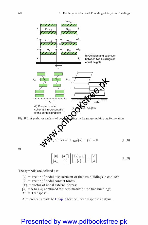
ruLðu; lÞ ¼ ½K�TOTfug � fdg ¼ 0 (10:8)
or
½K� ½KT00
l �½Kl� ½0�
" #fugTOT
flg
� �¼
F
d
� �(10:9)
The symbols are defined as:
{u} = vector of nodal displacement of the two buildings in contact;{l} = vector of nodal contact forces;{F} = vector of nodal external forces;[K] =A (n x n) combined stiffness matrix of the two buildings;T 00 = Transpose.
A reference is made to Chap. 5 for the linear response analysis.
(i) Collision and pushoverbetween two buildings ofequal heights
(ii) Coupled modelschematic representationof the contact problem
xg
ma,i mb,iua,i ub,ij l
m1,n
m2
m2,n–i k2
d
m1,n–i
m1
m1,n–i
m2,n
m2,n–ik2
k2
k2
k1
k1
(j–l)
k1
k1
(iii) Unequal heights
(a) (b)d
Fig. 10.1 A pushover analysis of buildings using the Lagrange multiplying formulation
606 10 Earthquake – Induced Pounding of Adjacent Buildings
www.pdfbo
oksfr
ee.pk
Presented by www.pdfbooksfree.pk
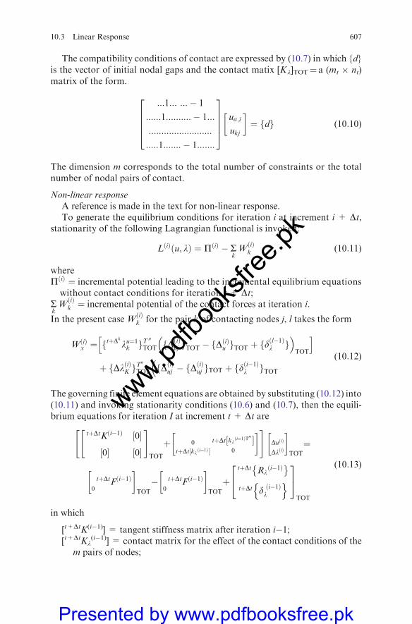
The compatibility conditions of contact are expressed by (10.7) in which {d}is the vector of initial nodal gaps and the contact matix [Kl]TOT¼ a (mt � nt)matrix of the form.
:::1::: :::� 1
::::::1:::::::::: � 1:::
:::::::::::::::::::::::::
:::::1::::::: � 1:::::::
26664
37775
ua;i
ukj
� �¼ fdg (10:10)
The dimension m corresponds to the total number of constraints or the totalnumber of nodal pairs of contact.
Non-linear responseA reference is made in the text for non-linear response.To generate the equilibrium conditions for iteration i at increment i + Dt,
stationarity of the following Lagrangian functional is invoked:
LðiÞðu; lÞ ¼ PðiÞ � SkWðiÞk (10:11)
wherePðiÞ ¼ incremental potential leading to the incremental equilibrium equationswithout contact conditions for iteration t + Dt;
SkWðiÞk ¼ incremental potential of the contact forces at iteration i.
In the present case WðiÞk for the pair k of contacting nodes j, l takes the form
WðiÞx ¼ ftþDk
lu¼1k gT 00
TOT fDðiÞuj gTOT � fDðiÞu gTOT þ fd
ðl�1Þl g
� �TOT
h i
þ fDlðiÞK gT00
TOT fDðiÞuj � fD
ðiÞuj gTOT þ fdði�1Þl gTOT
� (10:12)
The governing finite element equations are obtained by substituting (10.12) into(10.11) and invoking stationarity conditions (10.6) and (10.7), then the equili-brium equations for iteration I at increment t + Dt are
tþDtKði�1Þ 0½ �
0½ � 0½ �
" #TOT
þ 0
tþDt klði¼1Þ½ �tþDt klði¼1ÞT
00½ �0
� �" #DuðiÞ
DlðiÞ
� �TOT
¼
0
tþDtFði�1Þ� �
TOT
�0
tþDtFði�1Þ� �
TOT
þtþDt Rl
ði�1Þ� �tþDt d i�1ð Þ
l
n o24
35TOT
(10:13)
in which
[t+DtK(i�1)] = tangent stiffness matrix after iteration i�1;[t+DtKl
(i�1)] = contact matrix for the effect of the contact conditions of them pairs of nodes;
10.3 Linear Response 607
www.pdfbo
oksfr
ee.pk
Presented by www.pdfbooksfree.pk
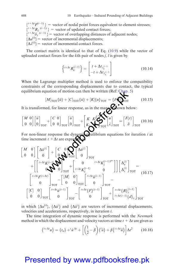
{t+DtF(i�1) } = vector of nodal point forces equivalent to element stresses;{t+DtRl
(i�1) } = vector of updated contact forces;{t+Dtdl
(i�1) }= vector of overlapping distances of adjacent nodes;{Du(i)}= vector of incremental displacements;{Dl(i)}= vector of incremental contact forces.
The contact matrix is identical to that of Eq. (10.9) while the vector ofuploaded contact forces for the kth pair of nodes j, l is given by
tþDtRi�1ð Þk
n o¼ tþ Dtl i�1ð Þ
k
�tþ Dtl i�1ð Þk
24
35 (10:14)
When the Lagrange multiplier method is used to enforce the compatibilityconstraints of the corresponding displacements due to contact, the typicalequilibrium equation of motion can then be written (Ref: Chap. 5)
M½ �TOT €uf g þ C½ �TOT _uf g þ K½ � uf gTOT ¼ F tð Þf gTOT (10:15)
It is transformed, for linear response, as in the manner shown below:
M 0
0 0
� �€u
0
� �TOT
þC 0
0 0
� �TOT
_u
0
� �TOT
þ K KT00
l
Kl 0
" #TOT
u
l
� �TOT
¼FðtÞd
� �TOT
(10:16)
For non-linear response the dynamic equilibrium equations for iteration i attime increment t +Dt are expressed as
M 0
0 0
� �D€uðiÞ
0
" #þ
C 0
0 0
� �TOT
D _uðiÞ
0
" #TOT
þtþDtKði�1Þ 0
0 0
" #TOT
þ0 tþDtK
ði�1ÞT00l
tþDtKði�1Þl 0
" #" #DðiÞu
DðiÞl
" #
TOT
¼
tþDtFðtþDtÞ
0
" #TOT
�½M� 0
0 0
� �TOT
tþDt€uði�1Þ
0
" #TOT
�
½C� 0
0 0
� �TOT
tþDt _uði�1Þ
0
" #TOT
�tþDtfFgði�1Þ
0
" #TOT
þtþDtfRgði�1ÞltþDtði�1Þfdgl
" #TOT
(10:17)
in which {Du(i)}, fD _uig and fD€uig are vectors of incremental displacements,velocities and accelerations, respectively, in iteration i.
The time integration of dynamic response is performed with the Newmarkmethod inwhich the displacement and velocity vectors at time t+Dt are given as
tþDtu� �
¼ tuf g þt _u Dt þ 1
2� b
� 0€uf g þ b tþDt€u
� �� �Dt2 (10:18)
608 10 Earthquake – Induced Pounding of Adjacent Buildings
www.pdfbo
oksfr
ee.pk
Presented by www.pdfbooksfree.pk
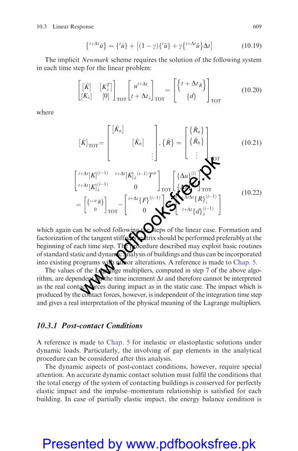
tþDt _u� �
¼ t _uf g þ 1� gð Þ t€uf g þ g tþDt€u� �
Dt �
(10:19)
The implicit Newmark scheme requires the solution of the following systemin each time step for the linear problem:
K �Kl½ �
KTl
�0½ �
" #
TOT
utþDt
tþ Dtl
" #TOT
¼tþ DtRn o
df g
24
35TOT
(10:20)
where
K �
TOT¼
Ka
�Kb
�...
26664
37775; ~R� �
¼
Ra
� �Rb
� �...
2664
3775TOT
(10:21)
tþDt K½ � i�1ð Þ tþDt K½ �l i�1ð ÞT 00
tþDt K½ � i�1ð Þl 0
" #
TOT
Duf g ið Þ
Dlf g ið Þ
" #
TOT
¼ tþDtRf g0
� �TOT
�tþDt Ff g i�1ð Þ
0
" #þ
tþDtDt Rf g i�1ð Þl
tþDt df g i�1ð Þl
" # (10:22)
which again can be solved following the steps of the linear case. Formation andfactorization of the tangent stiffnessmatrix should be performed preferably at thebeginning of each time step. The procedure described may exploit basic routinesof standard static and dynamic analysis of buildings and thus can be incorporatedinto existing programs with minor alterations. A reference is made to Chap. 5.
The values of the Lagrange multipliers, computed in step 7 of the above algo-rithm, are dependent on the time increment Dt and therefore cannot be interpretedas the real contact forces during impact as in the static case. The impact which isproduced by the contact forces, however, is independent of the integration time stepand gives a real interpretation of the physical meaning of the Lagrange multipliers.
10.3.1 Post-contact Conditions
A reference is made to Chap. 5 for inelastic or elastoplastic solutions underdynamic loads. Particularly, the involving of gap elements in the analyticalprocedure can be considered after this analysis.
The dynamic aspects of post-contact conditions, however, require specialattention. An accurate dynamic contact solution must fulfil the conditions thatthe total energy of the system of contacting buildings is conserved for perfectlyelastic impact and the impulse–momentum relationship is satisfied for eachbuilding. In case of partially elastic impact, the energy balance condition is
10.3 Linear Response 609
www.pdfbo
oksfr
ee.pk
Presented by www.pdfbooksfree.pk
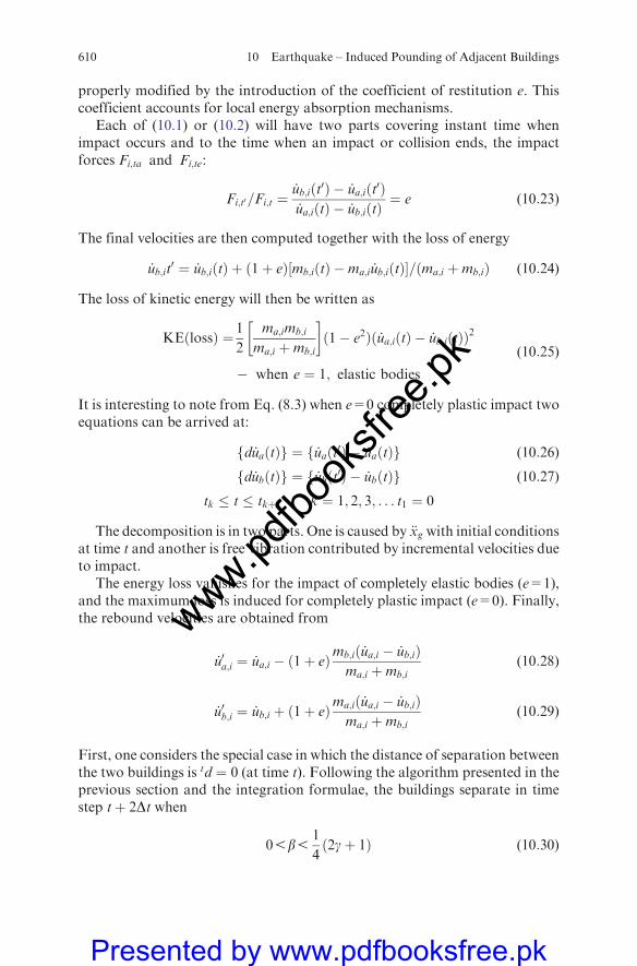
properly modified by the introduction of the coefficient of restitution e. Thiscoefficient accounts for local energy absorption mechanisms.
Each of (10.1) or (10.2) will have two parts covering instant time whenimpact occurs and to the time when an impact or collision ends, the impactforces Fi;ta and Fi;te:
Fi;t0=Fi;t ¼_ub;iðt0Þ � _ua;iðt0Þ_ua;iðtÞ � _ub;iðtÞ
¼ e (10:23)
The final velocities are then computed together with the loss of energy
_ub;it0 ¼ _ub;iðtÞ þ ð1þ eÞ½mb;iðtÞ �ma;i _ub;iðtÞ�=ðma;i þmb;iÞ (10:24)
The loss of kinetic energy will then be written as
KEðlossÞ ¼ 1
2
ma;imb;i
ma;i þmb;i
� �ð1� e2Þð _ua;iðtÞ � _ub;iðtÞÞ2
� when e ¼ 1; elastic bodies
(10:25)
It is interesting to note from Eq. (8.3) when e=0 completely plastic impact twoequations can be arrived at:
d _uaðtÞf g ¼ _uaðt0Þ � _uaðtÞf g (10:26)
d _ubðtÞf g ¼ _ubðt0Þ � _ubðtÞf g (10:27)
tk � t � tkþ1 k ¼ 1; 2; 3; . . . t1 ¼ 0
The decomposition is in two parts. One is caused by €xg with initial conditionsat time t and another is free vibration contributed by incremental velocities dueto impact.
The energy loss vanishes for the impact of completely elastic bodies (e=1),and the maximum loss is induced for completely plastic impact (e=0). Finally,the rebound velocities are obtained from
_u0a;i ¼ _ua;i � ð1þ eÞmb;ið _ua;i � _ub;iÞma;i þmb;i
(10:28)
_u0b;i ¼ _ub;i þ ð1þ eÞma;ið _ua;i � _ub;iÞma;i þmb;i
(10:29)
First, one considers the special case in which the distance of separation betweenthe two buildings is td ¼ 0 (at time t). Following the algorithm presented in theprevious section and the integration formulae, the buildings separate in timestep tþ 2Dt when
05b51
4ð2gþ 1Þ (10:30)
610 10 Earthquake – Induced Pounding of Adjacent Buildings
www.pdfbo
oksfr
ee.pk
Presented by www.pdfbooksfree.pk
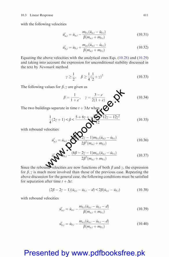
with the following velocities
_u0a;i ¼ _ua;i �mb;ið _ua;i � _ub;iÞbðma;i þmb;iÞ
(10:31)
_u0b;i ¼ _ub;i þma;ið _ua;i � _ub;iÞbðma;i þmb;iÞ
(10:32)
Equating the above velocities with the analytical ones Eqs. (10.28) and (10.29)and taking into account the expression for unconditional stability discussed inthe text by Newmark method
g � 1
2; b � 1
4ð12þ gÞ2 (10:33)
The following values for b; g are given as
b ¼ 1
1þ e; g ¼ 3� e
2ð1þ eÞ (10:34)
The two buildings separate in time tþ 3Dt when
1
4ð2gþ 1Þ5b5
5þ 6gþffiffiffiffiffiffiffiffiffiffiffiffiffiffiffiffiffiffiffiffiffiffiffiffiffiffiffiffiffiffiffiffiffi13þ 12g� 12g2
p12
(10:35)
with rebound velocities
_u0a;i ¼ _ua;i �ð6b� 2g� 1Þmb;ið _ua;i � _ub;iÞ
2b2ðma;i þmb;iÞ(10:36)
_u0b;i ¼ _ub;i �ð6b� 2g� 1Þma;ið _ua;i � _ub;iÞ
2b2ðma;i þmb;iÞ(10:37)
Since the rebound velocities are now functions of both b and g, the expressionfor b; g is much more involved than those of the previous case. Repeating theabove discussion for the general case, the following conditions must be satisfiedfor separation after time tþ Dt:
ð2b� 2g� 1Þð _ua;i � _ub;i � dÞ52bð _ua;i � _ub;iÞ (10:38)
with rebound velocities
_u0a;i ¼ _ua;i �mb;ið _ua;i � _ub;i � dÞ
bðma;i þmb;iÞ(10:39)
_u0b;i ¼ _ub;i �ma;ið _ua;i � _ub;i � dÞ
bðma;i þmb;iÞ(10:40)
10.3 Linear Response 611
www.pdfbo
oksfr
ee.pk
Presented by www.pdfbooksfree.pk
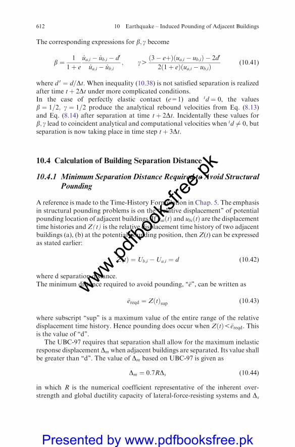
The corresponding expressions for b; g become
b ¼ 1
1þ e
_ua;i � _ub;i � d0
_ua;i � _ub;i; g4
ð3� eþÞðua;i � ub;iÞ � 2d0
2ð1þ eÞðua;i � ub;iÞ(10:41)
where d 0 ¼ d=Dt:When inequality (10.38) is not satisfied separation is realizedafter time tþ 2Dt under more complicated conditions.In the case of perfectly elastic contact (e=1) and td ¼ 0, the valuesb ¼ 1=2; g ¼ 1=2 produce the analytical rebound velocities from Eq. (8.13)and Eq. (8.14) after separation at time tþ 2Dt. Incidentally these values forb; g lead to coincident analytical and computational velocities when td 6¼ 0, butseparation is now taking place in time step tþ 3Dt.
10.4 Calculation of Building Separation Distance
10.4.1 Minimum Separation Distance Required to Avoid StructuralPounding
A reference is made to the Time-History Formulation in Chap. 5. The emphasisin structural pounding problems is on the ‘‘relative displacement’’ of potentialpounding location of adjacent buildings. If uaiðtÞ and ubiðtÞ are the displacementtime histories and Z(t) is the relative displacement time history of two adjacentbuildings (a), (b) at the potential pounding position, then Z(t) can be expressedas stated earlier:
ZðtÞ ¼ Ub;i �Ua;i ¼ d (10:42)
where d separation distance.The minimum distance required to avoid pounding, ‘‘�e’’, can be written as
�ereqd ¼ ZðtÞsup (10:43)
where subscript ‘‘sup’’ is a maximum value of the entire range of the relativedisplacement time history. Hence pounding does occur when ZðtÞ5�ereqd. Thisis the value of ‘‘d’’.
The UBC-97 requires that separation shall allow for the maximum inelasticresponse displacementDm when adjacent buildings are separated. Its value shallbe greater than ‘‘d’’. The value of Dm based on UBC-97 is given as
Dm ¼ 0:7RDs (10:44)
in which R is the numerical coefficient representative of the inherent over-strength and global ductility capacity of lateral-force-resisting systems and Ds
612 10 Earthquake – Induced Pounding of Adjacent Buildings
www.pdfbo
oksfr
ee.pk
Presented by www.pdfbooksfree.pk
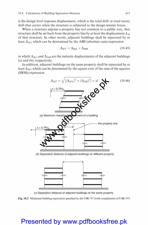
is the design level response displacement, which is the total drift or total storey
drift that occurs when the structure is subjected to the design seismic forces.When a structure adjoins a property line not common to a public way, that
structure shall be set back from the property line by at least the displacementDM
of that structure. In other words, adjacent buildings shall be separated by at
least DMT which can be determined by the ABS (absolute sum) expression
DMT ¼ DMA þ DMB (10:45)
in which DMA and DMB are the inelastic displacements of the adjacent buildings
(a) and (b), respectively.In addition, adjacent buildings on the same property shall be separated by at
least DMT which can be determined by the square root of the sum of the squares(SRSS) expression
DMT ¼ffiffiffiffiffiffiffiffiffiffiffiffiffiffiffiffiffiffiffiffiffiffiffiffiffiffiffiffiffiffiffiffiffiffiffiffiffiffi½ðDMAÞ2 þ ðDMBÞ2�
q¼ d (10:46)
(a) Maximum inelastic displacement of a building
(b) Separation distance of adjacent buildings on different property
Δ = 0.7RΔs
Δ = 0.7RΔs
the property line
(c) Separation distance of adjacent buildings on the same property
Fig. 10.2 Minimumbuilding separation specified by theUBC-97 (with compliments ofUBC-97)
10.4 Calculation of Building Separation Distance 613
www.pdfbo
oksfr
ee.pk
Presented by www.pdfbooksfree.pk
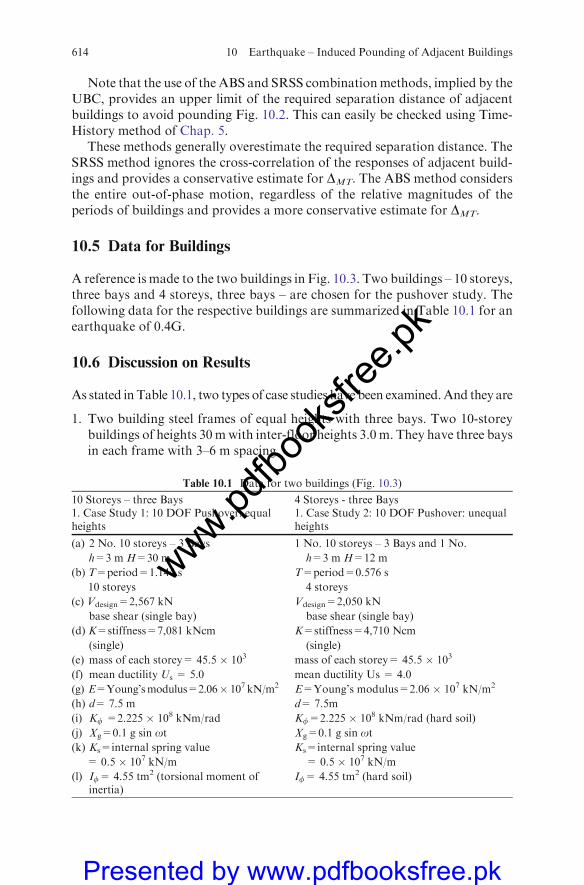
Note that the use of the ABS and SRSS combinationmethods, implied by theUBC, provides an upper limit of the required separation distance of adjacentbuildings to avoid pounding Fig. 10.2. This can easily be checked using Time-History method of Chap. 5.
These methods generally overestimate the required separation distance. TheSRSS method ignores the cross-correlation of the responses of adjacent build-ings and provides a conservative estimate for DMT. The ABS method considersthe entire out-of-phase motion, regardless of the relative magnitudes of theperiods of buildings and provides a more conservative estimate for DMT.
10.5 Data for Buildings
A reference is made to the two buildings in Fig. 10.3. Two buildings – 10 storeys,three bays and 4 storeys, three bays – are chosen for the pushover study. Thefollowing data for the respective buildings are summarized in Table 10.1 for anearthquake of 0.4G.
10.6 Discussion on Results
As stated in Table 10.1, two types of case studies have been examined.And they are
1. Two building steel frames of equal heights with three bays. Two 10-storeybuildings of heights 30mwith inter-floor heights 3.0 m. They have three baysin each frame with 3–6 m spacing.
Table 10.1 Data for two buildings (Fig. 10.3)
10 Storeys – three Bays 4 Storeys - three Bays1. Case Study 1: 10 DOF Pushover: equalheights
1. Case Study 2: 10 DOF Pushover: unequalheights
(a) 2 No. 10 storeys – 3 Bays 1 No. 10 storeys – 3 Bays and 1 No.
h=3 m H=30 m h=3 m H=12 m
(b) T=period=1.144 s T=period=0.576 s
10 storeys 4 storeys
(c) Vdesign=2,567 kN Vdesign=2,050 kN
base shear (single bay) base shear (single bay)
(d) K=stiffness=7,081 kNcm K=stiffness=4,710 Ncm
(single) (single)
(e) mass of each storey= 45.5 � 103 mass of each storey= 45.5 � 103
(f) mean ductility Us = 5.0 mean ductility Us = 4.0
(g) E=Young’smodulus=2.06� 107 kN/m2 E=Young’s modulus=2.06 � 107 kN/m2
(h) d= 7.5 m d= 7.5m
(i) Kf =2.225 � 108 kNm/rad Kf=2.225 � 108 kNm/rad (hard soil)
(j) Xg=0.1 g sin ot Xg=0.1 g sin ot(k) Ks=internal spring value Ks=internal spring value
= 0.5 � 107 kN/m = 0.5 � 107 kN/m
(l) If= 4.55 tm2 (torsional moment ofinertia)
If= 4.55 tm2 (hard soil)
614 10 Earthquake – Induced Pounding of Adjacent Buildings
www.pdfbo
oksfr
ee.pk
Presented by www.pdfbooksfree.pk
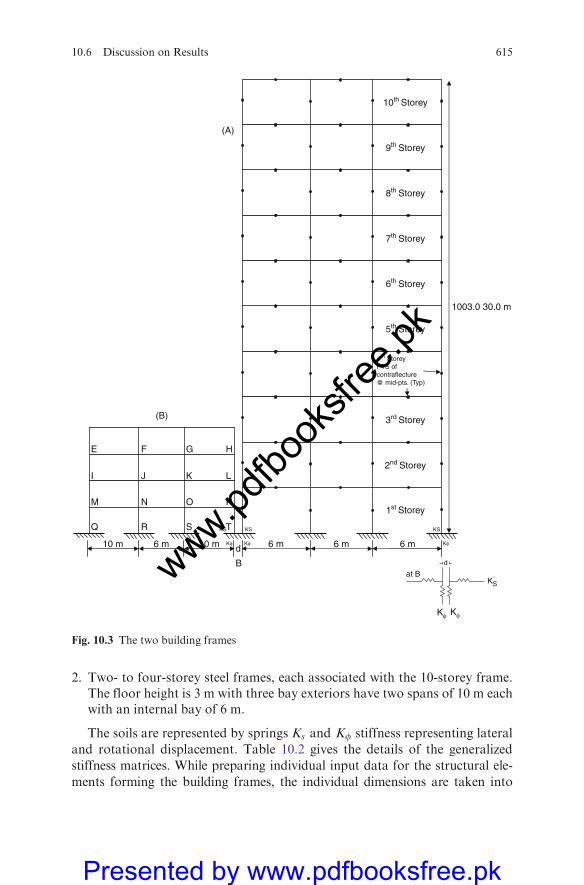
2. Two- to four-storey steel frames, each associated with the 10-storey frame.The floor height is 3 m with three bay exteriors have two spans of 10 m eachwith an internal bay of 6 m.
The soils are represented by springs Ks and Kf stiffness representing lateral
and rotational displacement. Table 10.2 gives the details of the generalized
stiffness matrices. While preparing individual input data for the structural ele-
ments forming the building frames, the individual dimensions are taken into
5th Storey
6th Storey
7th Storey
8th Storey
9th Storey
10th Storey
4th StoreyPTS ofcontraflecture@ mid-pts. (Typ)
E F G H
I J K
M
L
N O P
Q R S T KS KS
at B
Kφ Kφ
KS
KS
Kφ Kφ Kφ10 m 6 m6 m6 m10 m6 m
(B)
(A)
1003.0 30.0 m
d
B
3rd Storey
2nd Storey
1st Storey
d
Fig. 10.3 The two building frames
10.6 Discussion on Results 615
www.pdfbo
oksfr
ee.pk
Presented by www.pdfbooksfree.pk
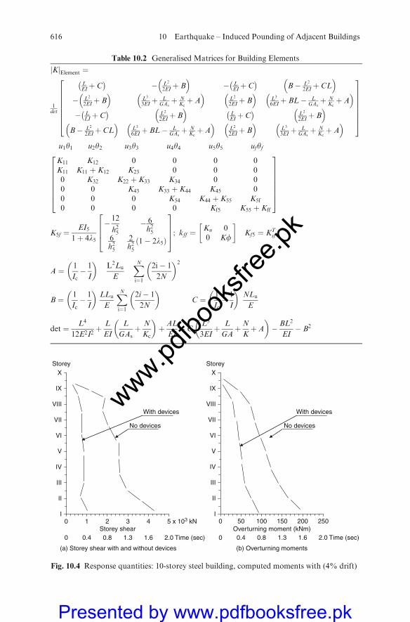
Table 10.2 Generalised Matrices for Building Elements
jKjElement ¼
1det
LEIþ C
�� L2
2EIþ B
� �� L
EIþ C
�B� L2
2EIþ CL
� �� L2
2EIþ B
� �L3
3EIþ L
GAsþ N
Kcþ A
� �L2
2EIþ B
� �L3
6EIþ BL� L
GAsþ N
Kcþ A
� �� L
LIþ C �
L2
2EIþ B
� �LEIþ C �
L2
2EIþ B
� �B� L2
2EIþ CL
� �L3
6EIþ BL� L
GAsþ N
Kcþ A
� �L2
2EIþ B
� �L3
3EIþ L
GAsþ N
Kcþ A
� �
26666664
37777775
u1y1 u2y2 u3y3 u4y4 u5y5 ufyf
K11 K12 0 0 0 0K11 K11 þ K12 K23 0 0 00 K32 K22 þ K33 K34 0 00 0 K43 K33 þ K44 K45 00 0 0 K54 K44 þ K55 K5f
0 0 0 0 Kf5 K55 þ Kff
26666664
37777775
K5f ¼EI5
1þ 4l5
� 12
h25� 6h25
6h25
2h25
1� 2l5ð Þ
2664
3775; kff ¼
Ku 00 Kf
� �Kf5 ¼ KT
sf
A ¼ 1
Ic� 1
I
� L2Lu
E
XNi¼1
2i� 1
2N
� 2
B ¼ 1
Ic� 1
I
� LLu
E
XNi¼1
2i� 1
2N
� C ¼ 1
Ic� 1
I
� NLu
E
det ¼ L4
12E2I2þ L
EI
L
GAsþ N
Kc
� þ AL
EIþ C
L3
3EIþ L
GAþN
Kþ A
� � BL2
EI� B2
5 x 10³ kN40
0.4
1 2 3I
Storey
0Storey shear
(a) Storey shear with and without devices (b) Overturning moments
II
III
IV
V
VI
VII
VIII
IX
X
0.8 1.3 1.6 2.0 Time (sec)
With devices
No devices
2502000
0.4
50 100 150I
Storey
0Overturning moment (kNm)
II
III
IV
V
VI
VII
VIII
IX
X
0.8 1.3 1.6 2.0 Time (sec)
With devices
No devices
Fig. 10.4 Response quantities: 10-storey steel building, computed moments with (4% drift)
616 10 Earthquake – Induced Pounding of Adjacent Buildings
www.pdfbo
oksfr
ee.pk
Presented by www.pdfbooksfree.pk
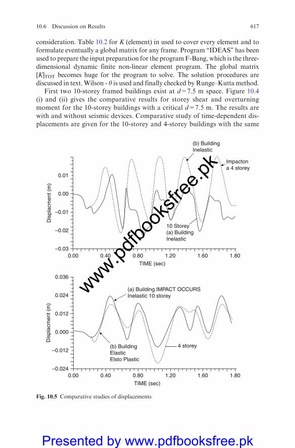
consideration. Table 10.2 for K (element) in used to cover every element and to
formulate eventually a global matrix for any frame. Program ‘‘IDEAS’’ has been
used to prepare the input preparation for the programF-Bang, which is the three-
dimensional dynamic finite non-linear element program. The global matrix
[K]TOT becomes huge for the program to solve. The solution procedures are
discussed in text.Wilson - y is used and finally checked by Runge–Kuttamethod.First two 10-storey framed buildings exist at d=7.5 m space. Figure 10.4
(i) and (ii) gives the comparative results for storey shear and overturning
moment for the 10-storey buildings with a critical d=7.5 m. The results are
with and without seismic devices. Comparative study of time-dependent dis-
placements are given for the 10-storey and 4-storey buildings with the same
–0.03
–0.02
–0.01
0.00
0.01
TIME (sec)
0.00 0.40 0.80 1.20 1.60 1.80
10 Storey(a) BuildingInelastic
Impactona 4 storey
(b) BuildingInelastic
–0.024
–0.012
0.000
0.012
0.024
TIME (sec)
0.00 0.40 0.80 1.20 1.60 1.80
(a) Building IMPACT OCCURSInelastic 10 storey
4 storey(b) BuildingElasticElsto Plastic
0.036
Dis
plac
men
t (m
)D
ispl
acm
ent (
m)
Fig. 10.5 Comparative studies of displacements
10.6 Discussion on Results 617
www.pdfbo
oksfr
ee.pk
Presented by www.pdfbooksfree.pk
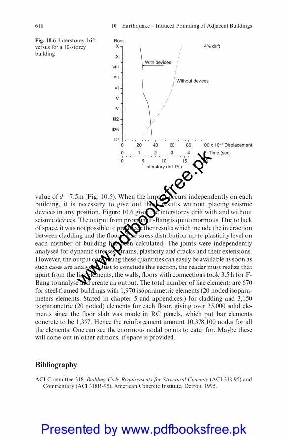
value of d=7.5m (Fig. 10.5). When the impact occurs independently on eachbuilding, it is necessary to give out these results without placing seismicdevices in any position. Figure 10.6 gives the interstorey drift with and withoutseismic devices. The output from programF-Bang is quite enormous. Due to lackof space, it was not possible to produce other results which include the interactionbetween cladding and the floors. The stress distribution up to plasticity level oneach member of building has been calculated. The joints were independentlyanalysed for dynamic stresses, strains, plasticity and cracks and their extensions.However, the output containing these quantities can easily be available as soon assuch cases are analysed. Just to conclude this section, the reader must realize thatapart from the line elements, the walls, floors with connections took 3.5 h for F-Bang to analyse and create an output. The total number of line elements are 670for steel-framed buildings with 1,970 isoparametric elements (20 noded isopara-meters elements. Stated in chapter 5 and appendices.) for cladding and 3,150isoparametric (20 noded) elements for each floor, giving over 35,000 solid ele-ments since the floor slab was made in RC panels, which put bar elementsconcrete to be 1,357. Hence the reinforcement amount 10,378,100 nodes for allthe elements. One can see the enormous nodal points to cater for. Maybe thesewill come out in other editions, if space is provided.
Bibliography
ACI Committee 318. Building Code Requirements for Structural Concrete (ACI 318-95) andCommentary (ACI 318R-95), American Concrete Institute, Detroit, 1995.
100 x 10–1 DisplacementI.2
Floor
Interstory drift (%)
II25
III2
IV
V
VI
VII
VIII
IX
X
5 Time (sec)
With devices
Without devices
800
1
20 40 60
0 2 3 4
200 5 10 15
4% driftFig. 10.6 Interstorey driftversus for a 10-storeybuilding
618 10 Earthquake – Induced Pounding of Adjacent Buildings
www.pdfbo
oksfr
ee.pk
Presented by www.pdfbooksfree.pk
Allahabadi, R., and Powell, G.H. DRAIN-2DX user guide. Report No. UCB/EERC-88/06,Earthquake Engineering Research Center, University of California, Berkeley, CA, 1988.
American Society of Civil Engineers. Prestandard and Commentary for the Seismic Rehabilita-tion of Buildings, FEMA-356, Federal EmergencyManagement Agency,Washington,DC,2000.
Anagnostopoulos, S.A. Building pounding re-examined: How serious a problem is it? Pro-ceedings of the 11th World Conference on Earthquake Engineering, Acapulco, Mexico,1996.
Anagnostopoulos, S.A. Earthquake induced pounding: State of the art. Proceedings of the10th European Conference on Earthquake Engineering 1995; Vol. 2: 897–905.
Anagnostopoulos, S.A. Pounding of buildings in series during earthquakes. Earthquake Eng.Struct. Dyn. 1988; 16:443–456.
Anagnostopoulos, S.A., and Spiliopoulos, K.V. An investigation of earthquake inducedpounding between adjacent buildings. Earthquake Eng. Struct. Dyn. 1992; 21:289–302.
Arnold, C., andReitherman, R.Building Configuration and Seismic Design.Wiley, NewYork,1982.
Athanasiadou, C.J., Penelis, G.G., and Kappos, A.J. Seismic response of adjacent buildingswith similar or different dynamic characteristics. Earthquake Spectra 1994; 10.
Aydinoglu, M.N. An incremental response spectrum analysis procedure based on inelasticspectral displacements for multi-mode seismic performance evaluation.Bullet. EarthquakeEng. 2003; 1:3–36.
Benjamin, J.R., and Cornell, C.A. Probability, Statistics, and Decision for Civil Engineers.McGraw-Hill, New York, 1970; 684pp.
Bertero, V.V. Observation on structural pounding. Proceeding of the International Conferenceon Mexico Earthquake, ASCE, 1986; 264–287.
Bracci, J.M., Kunnath, S.K., and Reinhorn, A.M. Seismic performance and retrofit evalua-tion for reinforced concrete structures. J. Struct. Eng. (ASCE) 1997; 123(1):3–10.
Building Seismic Safety Council. NEHRP Guidelines for the Seismic Rehabilitation of Build-ings, FEMA-273 and Commentary FEMA-274. Federal Emergency Management Agency,Washington, DC, 1997.
Chintanapakdee, C., and Chopra, A.K. Evaluation of modal pushover analysis for genericframes. Pacific Earthquake Engineering. Research Center, University of California,Berkeley, 2002, to be published.
Chintanapakdee, C., and Chopra, A.K. Evaluation of modal pushover analysis using genericframes. Earthquake Eng. Struct. Dyn. 2003; 32:417–442.
Chintanapakdee, C., Chopra, A.K. Seismic response of vertically irregular frames: Responsehistory and modal pushover analysis. J. Struct. Eng. (ASCE) 2004; 130(8), 1177–1185.
Chopra,A.K.Dynamic of Structures: Theory andApplications toEarthquakeEngineering (2nd ed.).Prentice-Hall, Englewood Cliffs, NJ, 2001; 844pp.
Chopra, A.K. and Goel, R. Modal pushover analysis of SAC building, Proceedings SEAOCConvention, San Diego, California, 2001.
Chopra, A.K., and Goel, R.K., A modal pushover analysis procedure to estimating seismicdemands for buildings: Theory and preliminary evaluation. PRREReport 2001/03, PacificEarthquake Research Center, University of California, Berkeley.
Chopra, A.K., and Goel, R.K., A modal pushover analysis procedure to estimating seismicdemands for buildings. Earthquake Eng. Struct. Dyn. 2002; 31: 561–582.
Chopra, A.K., and Goel, R.K. Capacity-demand-diagram methods based on inelastic designspectrum. Earthquake Spectra 1999; 15(4):637–656.
De Stefano, M., and Rutenberg, A. Predicting the dynamic response of asymmetrical multi-storey wall-frame structures by pushover analysis: Two case studies. Proceedings of the11th European Conference on Earthquake Engineering. Balkema Rotterdam, 1998.
Elnashai, A.S. Advanced inclastic static (pushover) analysis for earthquake applications.Struct. Eng. Mech. 2001; 12(1):51–69.
Bibliography 619
www.pdfbo
oksfr
ee.pk
Presented by www.pdfbooksfree.pk
Eurocode 2.Design of Concrete Structures- Part 1. General Rules and Rules for Building.CEN,Technical Committee 250/SG2, ENV 1992-1-1, 1991.
Eurocode 8.Structural in Seismic Regions, Design – Part 1. General and Building.CEC,ReportEUR 12266 EN, May 1994.
Fajfar, P., and Fischinger, M. N2- a method for nonlinear seismic analysis of regularstructures. Proceedings of the 9th World Conference on Earthquake Engineering, Tokyo-Kyoto, Japan, 1988; 5:111–116.
Goel, R.K., and Chopra, A.K. Period formulas for moment-resisting frame buildings. J.Struct. Eng. (ASCE) 1997; 123(11):1454–1461.
Gupta, A., and Krawinkler, H. Estimation of seismic drift demands for frame structures.Earthquake Eng. and Struct. Dyn. 2000; 29:1287–1305.
Gupta, B., and Kunnath, SK. Adaptive spectra-based pushover procedure for seismic evalua-tion of structures. Earthquake Spectra 2000; 16(2):367–392.
International Code Council. 2000 International Building Code. Falls Church, Virginia, 2000.Kilar, V., and Fajfar, P. Simple push-over analysis of asymmetric buildings. Earthquake Eng.
Struct. Dyn. 1997; 26:233–249.Kim, B, and D’Amore, E. Pushover analysis procedure in earthquake engineering. Earth-
quake Spectra 1999; 13:417–434.Krawinkler, H., and Seneviratna, GDPK. Pros and cons of a pushover analysis of seismic
performance evaluation. Engineering Structures 1998; 20:452–464.Krawinkler, H., and Nassar, A.A. Seismic design based on ductility and cumulative damage
demands and capacities. In Nonlinear Seismic Analysis and Design of ReinforcedConcrete Buildings (Fajfar, P. and Krawinkler, H., eds.). Elsevier Applied Science,New York, 1992.
Kunnath, S.K., and Gupta, B. Validity of deformation demand estimates using nonlinearstatic procedures. Proceedings of U.S. JapanWorkshop on Performance-Based EarthquakeEngineering Methodology for Reinforced Concrete Building Structures, Sapporo,Hokkaido, Japan, 2000; 117–128.
Maison, B. and Bonowitz, D. How safe are pre-NorthridgeWSMFs? A case study of the SACLos Angeles nine-storey building. Earthquake Spectra 1999; 25(1):31–46.
Matsumori, T., Otani, S., Shiohara, H., and Kabeyasawa, T. Earthquake member deforma-tion demands in reinforced concrete frame structures. Proceedings of U.S. –Japan Work-shop on Performance-Based Earthquake Engineering Methodology for Reinforced ConcreteBuilding Structures, Maui, Hawaii, 2000; 79–94.
Miranda, F. Seismic evaluation and upgrading of existing buildings. Ph.D. Dissertation,Department of Civil Engineering, University of California, Berkeley, CA, 1991.
Moghadam, A.S., and Tso, W.-K. Pushover analysis for asymmetrical multistorey buildings.Proceedings of the 6th U.S. National Conference on Earthquake Engineering, EERI,Oakland, CA, 1998.
Newmark, N.M., and Hall, W.J. Earthquake Spectra and Design. Earthquake EngineeringResearch Institute, Berkeley, CA, 1982; 103pp.
Ohtori, Y., Christenson, R.E, Spencer, Jr B.R, and Dyke, SJ. Benchmark Control Problemsfor Seismically Excited Nonlinear Buildings, http://www.nd.edu/�quake/, Notre DameUniversity, Indiana, 2000.
Paret, T.F., Sasaki, K.K., Eilbeck, D.H., and Freeman, S.A. Approximate inelastic proce-dures to identify failure mechanisms from higher mode effects. Proceedings of the 11thWorld Conference on Earthquake Engineering, Acapulco, Mexico, Paper No. 966, 1996.
Rosenblueth, E., and Meli, R. The 1985 earthquake: Causes and effects in Mexico City.Concrete Int. (ACI) 1986; 8(5):23–24.
Sasaki, K.K., Freeman, S.A., and Parent, T.F. Multimode pushover procedure (MMP) – amethod to identify the effects of higher modes in a pushover analysis. Proceedings of the6th U.S. National Conference on Earthquake Engineering, Seattle, Washington, 1998.
620 10 Earthquake – Induced Pounding of Adjacent Buildings
www.pdfbo
oksfr
ee.pk
Presented by www.pdfbooksfree.pk

Skokan, M.J., and Hart, G.C. Reliability of non-linear static methods for the seismic perfor-mance prediction of steel frame buildings. Proceedings of the 12th World Conference onEarthquake Engineering, Paper No. 1972, Auckland, New Zealand, 2000.
Vidie, T., Fajfar, P., and Fischinger, M. Consistent inelastic design spectra: Strength anddisplacement. Earthquake Eng. Struct. Dyn. 1994; 23(5):507–521.
Villaverde, R. Simplified response spectrum seismic analysis of non-liner structures. J. Struct.Eng. Mech., ASCE 1997; 123:256–265.
Westermo, B.D. The dynamic of interstructural connection to prevent pounding. EarthquakeEng. Struct. Dyn. 1989; 18:687–699.
Bibliography 621
www.pdfbo
oksfr
ee.pk
Presented by www.pdfbooksfree.pk

www.pdfbo
oksfr
ee.pk
Presented by www.pdfbooksfree.pk

Additional Extensive Bibliography
Analysis and Design of Buildings and Their Materials
1. ECCS Advisory Committee 1. Multi-storey Buildings in Steel – The Swedish Method(ECCS Publication No. 75). European Convention for Constructional Steelwork,Brussels, 1995.
2. Mullet, D. L. Slim Floor Design and Construction (SCI-Publication – 110). The SteelConstruction Institute, Ascot (Berkshire), 1992.
3. Mullet, D. L. and Lawson, R. M. Slim Floor Construction using Deep Decking (SCI-Publication-127). The Steel Construction Institute, Ascot (Berkshire), 1993.
4. Bogaard van de, A. W. A. M. J. and Eldik van, C. H. Verdiepingbouw in staal en beton-Staalskelet met geintegrerdde liggers en kanaalplaten (Multi-storey buildings in steel andconcrete-Steel frame with built-in beams and hollow core slabs, Dutch), StaalbouwInstituut, Rotterdam, 1995.
5. Eurocode 1. Basis of Design and Actions on Structures, Part 1: Basis of Design. CEN/TC250/N80, Draft July 1992.
6. Eurocode 3. Design of Steel Structures, Part 1.1: General Rules and Rules for Buildings.CEN, prENV, 1993-1-1.
7. ECCS Advisory Committee 5. Essentials of Eurocode 3. Design Manual for Steel Struc-tures in Building (ECCS Publication No. 65). European Convention for ConstructionalSteelwork, Brussels, 1991.
8. Verburg, W. H. Geintegreerde liggers-Rekenmodel voor de doorsnedecontrole volgensNEN 6770 (Built-in beams – Calculation model for member analysis according to theDutch code NEN 6770). Bouwen met Staal 1992; 107:7–12.
9. Wyatt, T. A. Design Guide on the Vibration of Floors (SCI-Publication -076). The SteelConstruction Institute, Ascot (Berkshire), 1989.
10. Precast Prestressed Hollow Core Floors (FIP Recommendations). Thomas Telford,London, 1988.
11. Anderson, J. Ljudisolering I bjalklag bestaende av stalbalk och haldackeselement (Soundinsulation in floor built-up from steel beam and hollow core slab, Swedish), SBI Rapport160: 1. Stalbyggnadsintute, Stockholm, 1992.
12. Anderson, J. Ljudisolering i bostadshus med stalstomme a (Sound insulation in residen-tial building with steel frame, Swedish), SBI Publikation 144. Stalbyggnadsinstitutet,Stockholm, 1992.
13. Eurocode 3.Design of Steel Structures, Part 1.2: Fire Resistance. CEN, prENV 1993-1-2.14. ECCS Technical Committee 3. European Recommendations for the Fire Safety of Steel
Structures. European Convention for Constructional Steelwork, Elsevier, Amsterdam/Brussels, 1983.
15. Saiidi, M. Constructability of Reinforced Concrete Joints. ACI Publication SCM-14 (86),Sec. VI, March 1986.
M.Y.H. Bangash, Earthquake Resistant Buildings,DOI 10.1007/978-3-540-93818-7, � M.Y.H. Bangash 2011
623
www.pdfbo
oksfr
ee.pk
Presented by www.pdfbooksfree.pk
16. Saiidi, M., Ghusn, G., and Jiang, Y. Five-spring element for biaxially bent R/C columns.J. Struct. Div. (ASCE) February 1989; 115:398–416.
17. Saiidi, M. and Sozen, M. A. Simple and Complex Models for Nonlinear Seismic Responseof Reinforced Concrete Structures. Civil Engineering Studies, Structural Research Seriesno 465, Department of Civil Engineering, University of Illinois, Urbana, 1979.
18. Sakino, K. and Ishibashi, H. Experimental Studies on Concrete Filled Square SteelTubular Short Columns Subjected to Cyclic Shearing Force and Constant Axial Force.Transactions of the Architectural Institute of Japan, no. 353, July 1985; 81–89.
19. Sakino, K. and Tomii, M. Hysteretic behavior of concrete filled square steel tubularbeam-columns failed in flexure. Transactions Japan Concrete Institute, 1981; 3:439–446.
20. Sakino, K., Tomii, M., andWatanabe, K. Sustaining load capacity of plain concrete stubcolumns confined by circular steel tube. Proc. Int. Specialty Conf. Concrete Filled SteelTubular Struct., Harbin, China, August 1985; 112–118.
21. SANZ. Code of Practice for the Design of Concrete Structures (NZS 3101 Part 1).Standards Association of New Zealand, Wellington, 1982.
22. Sargin, M. Stress-Strain Relationships for Concrete and Analysis of Structural ConcreteSections, Study no. 4. Solid Mechanics Division, University of Waterloo, Ontario,Canada, 1971.
23. Schickert, G. andWinkler, H. Results of Test Concerning Strength and Strain of ConcreteSubjected to Multiaxial Compressive Stress. Die Bundesanstalt fur Materialprufung(BAM), Berlin, Germany, 1977; p. 123.
24. Schlaich, J., et al. Toward a consistent design of structural concrete. PCI J. 1987; 2(3):74.25. Schlaich, J. and Schaefer, K. Konstruieren in Stahlbetonbau (Detailing in Reinforced
Concrete Design), Betonkalender, Part 2.W. Ernst, Berlin, Germany, 1984; pp. 787–1005.26. Schlaich, J., Schaefer, K., and Jennewein, M. Toward a consistent design of structural
concrete. PCI J. May–June 1987; 3:774–750.27. Schlaich, J. and Weischede, D. Detailing reinforced concrete structures. Proc. Can. Struct.
Concrete Conf., Department of Civil Engineering, University of Toronto, Toronto,Ontario, 1981; pp. 171–198.
28. Schmidt, W. and Hoffman, E. S. 9000 psi Concrete – Why? Why Not? Civil Engineering(ASCE), 1975; Vol. 45, pp. 52–55.
29. Schuster, J. Helical Stairs. Julius Hoffman, Stuttgart, Germany, 1964.30. Scott, B. D., Park, R., and Priestley, M. J. N. Stress-strain behavior of concrete by
overlapping hoops at low and high strain rates. ACI J. January–February 1982;79(1):13–27.
31. Scott, W. T., Reshoring aMultistory Concrete Frame: A Practical Approach, Analysis andDesign of High-Rise Concrete Buildings, ACI Special Publication SP-97. AmericanConcrete Institute, Detroit, 1985; pp. 277–301.
32. SEAOC.Recommended Lateral Force Requirements andCommentary. Structural Engineers’Association of California, San Francisco, 1975.
33. Sekin, M. and Uzumeri, S. M. Exterior beam-column joints in reinforced concreteframes. Proc. VIIth World Conf. Earthquake Eng., Istanbul, Turkey, September 1980;6:183–190.
34. Shah, S. P. New reinforced materials in concrete. ACI J. October 1974; 71(10):627.35. Shah, S. P. (ed.).Fatigue of Concrete Structures (ACI Special Publication SP-75). American
Concrete Institute, Detroit, 1982; pp. 133–175.36. Shah, S. P. and Rangan, B. V. Fiber reinforced concrete properties. ACI J. February
1971; 68(2):126–135.37. Shah, S. P., et al. Cyclic loading of spirally reinforced concrete. J. Struct. Eng. (ASCE)
July 1983; 109(ST7):1695–1710.38. Sheikh, S. A. and Uzumeri, S. M. Properties of Concrete Confined by Rectangular Ties.
Bulletin d’Inforamtion, no.132, Comite Euro-International du Beton, Paris, France,1979; pp. 53–60.
624 Additional Extensive Bibliography
www.pdfbo
oksfr
ee.pk
Presented by www.pdfbooksfree.pk

39. Sheikh, S. A. and Uzumeri, S. M. Strength and ductility of tied concrete columns.J. Struct. Div. (ASCE) May 1980; 106(ST5):1079–1102.
40. Siev, A. Analysis of free straight multiflight staircases. J. Struct. Div. (ASCE) 1962;88(ST3):207–232.
41. Smith, K.N. andVantsiotis, A. S. Shear strength of deep beams.ACI J. 1982; 79:201–213.42. Somerville, G. The Behavior and Design of Reinforced Concrete Corbels, Shear in Rein-
forced Concrete (ACI Special Publication SP-42). American Concrete Institute, Detroit,1974; pp. 477–502.
43. Stang, H. and Shah, S. P. Failure of fiber reinforced composites by pull-out fracture.J. Mater. Sci., March 1986; 21:953–957.
44. Steven, R. F. Encased stanchions. Struct. Eng. February 1965; 43(2):59–66.45. Suaris, W. and Shah, S. P. Properties of concrete and fiber reinforced concrete subjected
to impact loading. J. Struct. Div. (ASCE) July 1983; 103(ST7):1717–1741.46. Subedi, N. K. Reinforced concrete deep beams: a method for analysis. Proc. Inst. Civil
Eng. (London) 1988; 85:1–30.47. Paulay, T., Priestley, M. J. N., and Synge, A. J. Ductility in earthquake resisting squat
shear walls. ACI J. 1982; 79(4):257–269.48. Paulay, T. and Santhakumar, A. R. Ductile behaviour of coupled shear walls. J. Struct.
Div. (ASCE) 1976; 102(ST1):93–108.49. Paulay, T. and Taylor, R. G. Slab coupling of earthquake resisting shear walls. ACI J.
1981; 78(2):130–140.50. Paulay, T. and Uzumeri, S. M. A critical review of the seismic design provisions for
ductile shear walls of the Canadian code and commentary. Can. J. Civ. Eng.1975;2(4)592–601.
51. Pfeifer, D. W., Magura, D. D., Russell. H. G., and Corley, W. G. Time DependentDeformations in a 70 Story Structure, Designing for Effects of Creep and Shrinkage inConcrete Structures (ACI Special Publication SP-76). American Concrete Institute,Detroit, 1971; pp. 159–185.
52. Portland Cement Association. Design of Deep Girders (Publication ISO79.01D). PCA,Skokie, III, 1980.
53. Potucek,W. Die Beanspruchung der Stege von Stablbetonplattenbalken durch Querkraftund Biegung (Stresses inWebs of Reinforced Concrete T-Beams Subjected to Flexure andShear). Zement und Beton 1977; 22(3):88–98.
54. Potyondy, J. G. Concrete filled tubular steel structures in marine environment. Proc. Int.Specialty Conf. Concrete Filled Steel Tubular Struct., Habin, China, August 1985; 27–31.
55. Priestley, M. J. N. and Park, R. Strength and Ductility of Bridge Substructures. ResearchReport 84-20, Department of Civil Engineering, University of Canterbury, Christchurch,New Zealand, 1984; 120.
56. Priestley, M. J. N., and PARK , R. J. N., Concrete Filled Steel Tubular Piles underSeismic Loading, Proceedings of the International Specialty Conference on ConcreteFilled Steel Tubular Structures, Harbin, China, August 1985; pp. 96–103.
57. Priestley, M. J. N., Park, R., and Potangaroa, R. T. Ductility of spirally-confinedconcrete columns. J. Struct. Div. (ASCE) January 1981; 107(ST1):181–202.
58. PTI. Design of Post-Tensioned Slabs. Post-Tensioning Institute, Glenview, III, 1984.59. Ragan, H. S. and Warwaruk, J. Tee members with large web openings. PCI J. August
1967; 12(4):52–65.60. Ramakrishnan, V. and Ananthanarayana, Y. Ultimate strength of deep beams in shear.
ACI J. 1968; 65:87–98.61. Ramakrishnan, V. and Josifek, C. performance characteristics and flexural fatigue
strength on concrete steel fiber composites. Proc. Int. Symp. Fiber Reinforced Concrete,Madras, India, Oxford and IBH Publishing, New Delhi, December 1987; pp. 2.73–2.84.
62. Ramakrishnan, V., et al. A compressive evaluation of concrete reinforced straight steelfibres with deformed ends glued together bundles.ACI J.May–June 1980; 77(3):135–143.
Additional Extensive Bibliography 625
www.pdfbo
oksfr
ee.pk
Presented by www.pdfbooksfree.pk

63. Rausch, E. Design of inclined reinforcement to resist direct shear; Direct shear in concretestructures. Der Bauingenieur (Heidelberg) April 1922; 3(7):211–212; August 1931; 12(32/33):257.
64. Raush, E.Design for shear in reinforced concrete structures.Der Bauingenieur (Heidelberg)1963; 38:257.
65. Rawdon de paiva, H. A. and Siess, C. P. Strength and behavior of deep beams in shear.J. Struct. Div. (ASCE) 1965; 91:19–41.
66. Regan, P. E. Shear in RC beams. Mag. Concrete Res. March 1969; 21(66):31–42.67. Reinhardt, H. W. and Walraven, J. C. Cracks in concrete subject to shear. J. Struct. Div.
(ASCE) January 1982; 108(ST1):207–224.68. Rice, P. F. and Hoffman, E. S. Structural Design Guide to the ACI Building Code. Van
Nostrand Reinhold, New York, 1985.69. Ritter, W. Die Beauweise Hennebique (Hennebique’s construction method). Schweizerische
Bauzeitung (Zurich) 1899; 17:41–43, 49–52, 59–61.70. Rogowsky, D. M. and Macgregor, J. G. The design of reinforced concrete deep beams.
Concrete Int.: Design Construct. 1986; 8(8):49.71. Rogowsky, D. M., Macgregor, J. G., and Ong, S. Y. Test of reinforced concrete deep
beams. ACI J. July–August 1986; 83(4):614–623.72. Roik, K., Bergmann, R., Bode, H., and Wagenknecht, G. Tragfahigkeit von ausbeto-
nierten Hohlprofilstutzen aus Baustahl, Technical Report no. 75-4, Institut fur Kon-struktiven Ingenieurbau, Ruhr-Universitat Bochum, Germany, May 1975.
73. Romualdi, J. P. and Baston, G. R. Mechanics of crack arrest in concrete. J. Eng. Mech.Div. (ASCE) June 1963; 89(EM3):147–168.
74. Romualdi, J. P. and Mandeo, J. A. Tensile strength of concrete affected by uniformlydistributed and closely spaced short lengths of wire reinforcement. ACI J. June 1964;61(6):657–670.
75. Rosman, H. G. Approximate analysis of shear walls subjected to lateral loads. ACI J.1964; 61:717–733.
76. Russell, H. G. High-rise Concrete Buildings: Shrinkage, Creep, and Temperature Effects,Private Communication, 1985.
77. Saenz, L. P. and Martin, I. Slabless tread-riser stairs. ACI J. 1961; 58:353.78. Mattock, A. H. Design proposals for reinforced concrete corbels. PCI J. May–June 1976;
21(3):8–42.79. Mattock, A. H., et al. The behavior of reinforced concrete corbels. PCI J. March–April
1976; 21(2):52–77.80. Mayfield, B., Kong, F. K., Bennison, A., and Davies, J. C. D. T. Corner joint details in
structural lightweight concrete. ACI J. May 1971; 68(5):366–372.81. Mccormac, C. W. Design of Reinforced Concrete, 2nd edn. Harper & Row, New York,
1986; Chapter 14.82. Mehmel, A. and Freitag, W. Tests on the load capacity of concrete brackets (in German).
Der Bauingenieur (Heidelberg) 1967; 42(10):362–369.83. Meinheit, D. F. and Jirsa, J. O. Shear strength of reinforced concrete beam-column
connections. J. Struct. Div. (ASCE) 1983; 107(ST11):2227–2244.84. Meyers, V. J. Matrix Analysis of Structures. Harper & Row, New York, 1983.85. Mindess, S. The Fracture of Fiber Reinforced and Polymer Impregnated Concretes: A
Review, Fracture Mechanics of Concrete. Elsevier Applied Science Publishers, Amster-dam, The Netherlands, 1983; pp. 481–501.
86. Mindess, S. and Young, J. F. Concrete. Prentice Hall, Englewood Cliffs, NJ, 1981;Chapter 18.
87. Mitchell, D. and Collins, M. P. Diagonal compressions field theory – a rational model forstructural concrete in pure torsion. ACI J. August 1974; 71(8):396–408.
88. Mitchell, D. andCook,W.D. Preventing progressive collapse of slab structures. J. Struct.Eng. (ASCE) July 1984; 110(ST7):1513–1532.
626 Additional Extensive Bibliography
www.pdfbo
oksfr
ee.pk
Presented by www.pdfbooksfree.pk

89. Mochle, J. P., Diebold, J. W., and Zee, H. L. Experimental study of a flat- plate buildingmodel. Proc. 18thWorld Conf. Earthquake Eng., San Francisco, CA, July 1984; Vol. IV,pp. 355–362.
90. Moersch, E., Der Eisenbetonbau-Seine Theorie und Anwendung (Reinforced ConcreteConstruction-Theory and Application), 3rd edn. K. Wittwer, Stuttgart, 1908; 5th edn.,Vol. 1, Part 2, 1922.
91. Moersch, E. Concrete Steel Construction, English translation by E. P. Goodrich.McGraw-Hill, New York, 1909; 368 pp. (Translation from 3rd edition of Der Eisen-bentonbau; 1st edition 1902).
92. Mohammadi, J. and Yazbeck, G. J. Strategies for Bridge Inspection using probabilisticmodels. Structural Safety and Reliability (Aug, A. H.-S., Shinozuka, M., and Schueller,G. I., eds.). American Society of Civil Engineers, New York, 1990; Vol. 3, pp. 2115–2122.
93. Mokhtar, A. S., et al. Stud shear reinforcement for flat concrete plates. ACI J. September–October 1985; 82(5):676–683.
94. Moretto, O. Reinforced Concrete Course (Curso de Hormingon Armado), 2nd edn.Libreria El Ateneo, Buenos Aires, Argentina, 1971.
95. Moretto, O.Deep Foundations – Selected Synthesis of the Present State of the Knowledgeabout Soil Integration. Revista Latinoamericana de Geotecnia, Caracas, Venezuela,July–September, 1975.
96. Moretto, O. Foundations of the bridges over the Parana River in Argentina. Proc. 5thPan American Conf. Soil Mech. Found. Eng., Buenos Aires, Argentina, 1975; Vol. v.
97. Morishita, Y., Tomii, M., and Yoshimura, K. Experimental studies of bond strength inconcrete filled circular steel tubular columns subjected to axial loads.Transactions JapanConcrete Institute 1979; 1:351–358.
98. Morishita, Y., Tomii, M., and Yoshimura, K. Experimental studies on bond strength inconcrete filled square steel tubular columns subjected to axial loads. Transactions JapanConcrete Institute, 1979; 1:359–366.
99. Morishita, Y. and Tomii, M. Experimental studies on bond strength between squaresteel tube and encased concrete core under cyclic shearing force and constant axial force.Transactions Japan Concrete Institute 1982; 4:363–370.
100. Morrison, D. G. and Sozen, M. A. Response of Reinforced Concrete Plate-Column Con-nections to Dynamic and Static Horizontal Loads. Civil Engineering Studies, StructuralResearch Series no. 490, University of Illinois, Urbana, April 1981.
101. Morrison, J. K., et al. Analysis of the debonding and pull-out process in frame compo-sites. J. Eng. Mech. Div. (ASCE) February 1988; 114:277–294.
102. Mphonde, A. C. and Frantz, G. C. Shear Test of High- and Low- strength ConcreteBeams with Stirrups (ACI Special Publication SP-87). American Concrete Institute,Detroit, pp. 179–196.
103. Mueller, P. Failure Mechanisms for Reinforced Concrete Beams in Torsion and Bending.International Association for Bridge and Structural Engineering Publications, 1976;Vol. 36, pp. 147–163.
104. Naaman, A. E. and Shah, S. P. Pullout mechanism in steel fiber reinforced concrete.J. Eng. Mech. Div. (ASCE) August 1976; 102(ST8):1537–1548.
105. Naaman, A. E., et al. Probabilistic analysis of fiber reinforced concrete. J. Eng. Mech.Div. (ASCE) April 1974; 100(EM2):397–413.
106. Nasser, K. W., Acavalos, A., and Daniel, H. R. Behavior and design of large opening inreinforced concrete beams. ACI J. January 1967; 64(1):25–33.
107. Mansur, M. A., et al. Ultimate torque of R/C beam with large openings. J. Struct. Eng.(ASCE) August 1983; 109(8):2602–2618.
108. Mansur, M. A., et al. Collapse loads of R/C beams with large openings. J. Struct. Eng.(ASCE) November 1984; 110(11):1887–1902
109. Mansur, M. A., et al. Design method for reinforced concrete beams with large openings.ACI J. July–August 1985; 82(4):517–524.
Additional Extensive Bibliography 627
www.pdfbo
oksfr
ee.pk
Presented by www.pdfbooksfree.pk

110. Marti, P., Zur Plastischen Berechnung von Stahlbeton (on Plastic Analysis of ReinforcedConcrete). Institute of Structural Engineering, ETH Zurich, Switzerland, 1980; Reportno. 104, 176 pp.
111. Marti, P. Strength and Deformations of Reinforced Concrete Members under Torsion andCombined Actions. Bulletin d’information, no. 146. Comite Euro-International duBeton, January 1982; pp. 97–138.
112. Marti, P. Basic tools of reinforced concrete beam design. ACI J. January–February1985; 82:46–56; also, Discussion November–December 1985; 82(6):933–935.
113. Marti, P. Truss models in detailing.Concrete International: Design ConstructionOctober1985; 8(10):66–68.
114. Marti, P. Staggered shear design of simply supported concrete beams. ACI J. January–February 1986; 83(1):36–42.
115. Marti, P. Staggered shear design of concrete bridge girders. Proc. Int. Conf. ShortMedium Span Bridges, Ottawa, ON, Canada, August 1986; Vol. 1, pp. 139–149.
116. Marti, P. Design of concrete slabs for transverse shear. ACI Struct. J. 1986; 84(1).117. Marti, P. Personal Communication, 1990.118. Marti, P. and Kong, K. Response of reinforced concrete slab elements to torsion.
J. Struct. Eng. (ASCE) May 1987; 113(ST5):976–993.119. Martinez, S., Nilson, A. H., and Slate, F. O. Spirally-reinforced high-strength
concrete columns. ACT J. September–October 1982; 81:431–442; Research reportno. 82-101, Department of Structural Engineering, Cornell University, Ithaca, NY,August, 1982.
120. Mast, R. F. Auxiliary reinforced in concrete connections. ASCE Proc. June 1968;94(ST6):1485–1504.
121. Matsui, C. strength and behavior of frames with concrete filled square steel tubularcolumns under earthquake loading. Proc. Int. Specialty Conf. Concrete Filled SteelTubular Struct., Harbin, China, August 1985; pp. 104–111.
122. Matsui, C. Local bucking of concrete filled steel square tubular columns. IABSE-ECCSSymp., Luxembourg, September 1985; pp. 269–276.
123. Kotsovos, M. D. An analytical investigation of the behavior of concrete under concen-tration of load. Mater. Struct. (RILEM) September–October 1981; 14(83):341–348.
124. Kotsovos, M. D. A fundamental explanation of the behavior of RC beams in flexurebased on the properties of concrete under multiaxial stress. Mater. Struct. (RILEM)November–December 1982; 15:529–537.
125. Kotsovos, M. D. Effect of testing techniques on the post-ultimate behavior of concretein compression. Mater. Struct. (RILEM) 1983:16:3–12.
126. Kotsovos, M. D. Mechanisms of ‘shear’ failure. Mag. Concrete Res. June 1983;35(123):99–106.
127. Kotsovos, M. D. Behavior of RC beams with shear span to depth ratios between 1.0 and2.5. ACI J. May–June 1984; 81(3):279–286.
128. Kotsovos, M. D. Deformation and failure of concrete in a structure. Int. Conf. ConcreteUnder Multiaxial Conditions (RILEM-CEB-CNRS), Toulouse, France, May 1984.
129. Kotsovos, M. D. Behavior of reinforced concrete beams with a shear span to depth ratiogreater than 2.5. ACI J. 1986; 83:1026–1034.
130. Kotsovos, M. D. Shear failure of reinforced concrete beams. Eng. Struct. 1987; 9:32–38.131. Kotsovos, M. D. Shear Failure of RC Beams: A Reappraisal of Current Concepts.
Bulletin, d’information, no. 178/179. Comite Euro-International du Beton, Paris,France, 1987; pp. 103–112.
132. Kotsovos, M. D. Compressive force path concept: basis for ultimate limit state reinforcedconcrete design. ACI J. 1988; 85:68–75.
133. Kotsovos,M.D. Design of reinforced concrete deep beams. Struct. Eng. 1988; 66:28–32.134. Kotsovos, M. D. Designing RC beams in compliance with the concept of the compressive
force path (in preparation).
628 Additional Extensive Bibliography
www.pdfbo
oksfr
ee.pk
Presented by www.pdfbooksfree.pk

135. Kotsovos, M. D. Behavior of RC beams designed in compliance with the compressiveforce path (in preparation).
136. Kotsovos, M. D. Shear failure of RC beams (in preparation).137. Kotsovos, M. D. Behavior of RC beams with shear span to depth ratios greater than 2.5
(in preparation).138. Kotsovos, M. D. The Use of Fundamental Properties of Concrete for the Design of RC
Structural Members. Research Project Sponsored by Nuffield Foundation, Award No.890BA, Imperial College.
139. Hillerborg, A. Analysis of fracture by means of the fictitious crack model. Int. J. CementComposite 1980; 2:177–184.
140. Hoff, G. C. Bibliography on fiber reinforced concrete. Proc. Int. Symp. Fiber ReinforcedConcrete, Madras, India, Oxford and IHB Publishing, New Delhi, December 1987;pp. 8.3–8.163.
141. Hognestad, E., A Study of Combined Bending and Axial Loading in Reinforced ConcreteMembers. Bulletin no. 399, Engineering Experiment Station, University of Illinois,Urbana, November 1951.
142. Holmes,M. andMartin, L. H.Analysis andDesign of Structural Connections, ReinforcedConcrete and Steel. Ellis Horwood Ltd., West Sussex, UK, 1983
143. Hsu, T. T. C. Softened truss model theory for shear and torsion. ACI Struct. J.November–December 1988; 85(6):624–635.
144. Hurd, M. K. Formwork for Concrete, 4th edn. ACI Special Publication SP-4, AmericanConcrete Institute, Detroit, 1979.
145. Hurd, M. K. and Courtois, P. D. Method of analysis for shoring and reshoringin multistory buildings. Second Int. Conf. Forming Econ. Concrete Building,ACI Special Publication, SP-90, American Concrete Institute, Detroit, 1986;pp. 91–100.
146. IABSE. Colloquium on Plasticity in Reinforced Concrete. International Association ofBridge and Structural Engineers, Copenhagen, Introductory Report, Vol. 28, 172 pp,Final Report, Vol. 29, 360 pp., 1979.
147. IAEE. Earthquake Resistant Regulations – A World List. International Association forEarthquake Engineers, Tokyo, Japan, 1984; p. 904.
148. Iqbal, M. and Derecho, A. T. Inertial Forces over Height of Reinforced ConcreteStructural Walls During Earthquakes, Reinforced Concrete Structures Subjected toWind and Earthquake Forces. ACI Special Publication SP-63, American Concrete Insti-tute, Detroit, 1980; pp. 173–196.
149. Japan Concrete Institute. Method of Test for Flexural Strength and Flexural Toughnessof Fiber Reinforced Concrete. Japan Concrete Institute, 1983; pp. 45–51.
150. Jeng, Y. S. and Shah, S. P. Crack propagation of steel fiber reinforced mortar andconcrete. Proc. Int. Symp. Fibrous Concrete CI, The Construction Press Ltd., Lancaster,UK, 1986.
151. Johnston, C.D. Properties of steel fiber reinforcedmortar and concrete.Proc. Int. Symp.Fibrous Concrete CI, The Construction Press Ltd., Lancaster, UK, 1980.
152. Johnston, C. D. Definition and measurements of flexural toughness parameters offiber reinforced concrete. Cement Concrete Aggr. CCAGDP, ASTM (Winter) 1982;4(2):53–60.
153. Johnston, C. D. Steel fiber reinforced concrete – present and future in engineeringconstruction. J. Composites April 1982; pp. 113–121.
154. Johnson, E. and Savre, T. I. Tests on Brackets in Concrete (in Norwegian). NorwegianBuilding Research Institute, Oslo, Report no. 2/1976, 1976; p. 31.
155. Kaba, S. A. and Mahin, S. A. Refined Modeling of Reinforced Concrete Columns forSeismic Analysis. Earthquake Engineering Research Center, University of California,Berkeley, Report no. UCB/EERC-84/03, April 1984.
Additional Extensive Bibliography 629
www.pdfbo
oksfr
ee.pk
Presented by www.pdfbooksfree.pk

156. Kani, G. N. J. The riddle of shear and its solution. ACI J. April 1964; 61(4):441–467.157. Karshenas, S. and Ayoub, H. An investigation of live loads on concrete structures
during construction. Proc. I COSSAR’89, 5th Int. Conf. Struct. Safety Reliability, SanFrancisco, CA, 1989; pp. 1807–1814.
158. Kato, B., Akiyama, H., and Kitazawa, S. Deformation Characteristics of Box-shapedSteel Members Influenced by Local Buckling (in Japanese). Transactions Architect. Inst.Jpn. June 1978; 268:71–76.
159. Kienberger, H.DiaphragmWalls as Load Bearing Foundations. Institute of Civil Engineers,London, UK, 1975.
160. Kemp, E. L. and Mukherjee, P. R. Inelastic behavior of corner knee joints. ConsultingEngineer, October 1968; pp. 44–48.
161. Knowles. R. B. and Park, R. Strength of concrete filled steel tubular columns. J. Struct.Div. (ASCE) December 1969; 95(ST12):2565–2587.
162. Kollegger, J. and Mehlhorn, G. Material model for cracked reinforced concrete. Proc.IABSE Colloquium Comput. Mech. Concrete Struct., Delft, The Netherlands, August1987; pp. 63–74.
163. Kong, F. K. and Evans, R. H. Reinforced and Prestressed Concrete, 2nd edn. TheEnglish Language Book Society and Nelson, 1980, pp. 162–179.
164. Kong. F. K., Robins, P. J., and Cole, D. F. Web reinforcement effects on deep beams.ACI J. 1970; 67:1010–1017.
165. Kong, F. K., et al. Design of reinforced concrete deep beams in current practice. Struct.Eng. 1975; 53(4):73–180.
166. Kormeling, H. A., et al. Static and fatigue properties of concrete beams reinforced withcontinuous bars and with fibers. ACI J. January–February 1980; 77(1):36–43.
167. Kotsovos, M. D. Fracture processes of concrete under generalized stress states. Mater.Struct. (RILEM) November–December 1979; 12(72):431–437.
168. ACI Committee 207. ACI Manual of Concrete Practice, Part 1, 1986.169. ACI Committee 209. Prediction of creep, shrinkage, and temperature effects in concrete
structures. Designing for Creep and Shrinkage in Concrete Structures (ACI SpecialPublication SP-76). American Concrete Institute, Detroit, 1982; pp. 139–300.
170. ACI 228. In-place methods for determination of strength of concrete, American Con-crete Institute. ACI Mater. J. September–October 1988; F85(5):446–471.
171. ACI. Building Code Requirements for Reinforced Concrete (ACI 318–83). AmericanConcrete Institute, Detroit, 1983.
172. ACI Committee 318. Building Code Requirements for Reinforced Concrete. AmericanConcrete Institute, Detroit, 1983; 111 pp.
173. ACI 318. Building Code Requirements for Reinforced Concrete (ACI 318–89) andCommentary (ACI 318R–89). American Concrete Institute, Detroit, 111 pp., 1989.
174. ACI 347. Recommended Practice for Concrete Formwork. American Concrete Institute,Detroit, 1978; 37 pp.
175. ACI 363. State-of-the-art on high strength concrete. ACI J. July–August 1984;81(4):364–411.
176. ACI Committee 544. State of the art report on fiber reinforced concrete. ACI J.November 1973; 70(11):729–744.
177. ACI Committee 544. Measurements of properties of fiber reinforced concrete. ACI J.July 1978; 75(7):283–289.
178. ACI Committee 544. Measurements of properties of fiber reinforced concrete. ACI J.November–December, 1988; pp. 583–593.
179. ACI-ASCE Committee 352. Revised recommendations for the Design of Beam-ColumnJoints. American Concrete Institute, Detroit, draft. No. 11, 1984; 34 pp.
180. ACI-ASCE Committee 352. Recommendations for design of beam-column jointsin monolithic reinforced concrete structures. ACI J. May–June 1985; 82(3):266–283.
630 Additional Extensive Bibliography
www.pdfbo
oksfr
ee.pk
Presented by www.pdfbooksfree.pk

181. Computational mechanics of concrete structures: advances and applications. Transac-tions of IABSE Colloquium Delft 87, Delft, August 1987; pp. 113–120.
182. Pruijssers, A. F. Shear resistance of cracked concrete subjected to cyclic loading. Compu-tational Mechanics of Concrete Structures: Advances and Applications, Transactions ofIABSE Colloquium Delft 87, Delft, August 1987; pp. 43–50.
183. Walraven, J. C. Aggregate interlock under dynamic loading. Darmstadt Concrete 1986;1:143–156.
184. Yoshikawa H. et al. Analytical model for shear slip of cracked concrete. J. Struct. Eng.Am. Soc. Civ. Engrs. April 1989; 115(4):771–788.
185. Li, B. and Maekawa, K. Contact density model for cracks in concrete. Computationalmechanics of concrete structures: advances and applications. Transactions IABSEColloquium Delft August 1987; 87:51–62.
186. Bazant, Z. P. and Gambarova, P. G. Crack shear in concrete: crack band micro planemodel. J. Struct. Eng. Am. Soc. Civ. Engrs September 1984; 110(9):2015–2035.
187. Riggs, H. R. and Powell, G. H. Rough crack model for analysis of concrete. J. Eng.Mech. (ASCE) May 1986; 112(5):448–464.
188. Bazant, Z. P. and Oh, B. H. Microplane model for progressive fracture of concrete androck. J. Eng. Mech. (ASCE) 1985; 111(4):559–582.
189. Gambarova, Z. P. and Floris, E. Microplane model for concrete subject to planestresses. Nucl. Eng. Design 1986; 97:31–48.
190. Bazant, Z. P. and Prat, P. C. Microplane model for brittle-plastic material: I. Theory;II. Verification. J. Eng. Mech. (ASCE) 1988; 114(10):1672–1702.
191. Feensra, P. H., et al. Numerical study on crack dilatancy. I. Models and Stabilityanalysis; II. Applications. J. Eng. Mech. (ASCE) April 1991; 117(4):733–753, 754–769.
192. Cedolin, L. and Dei Poli, S. Finite element studies of shear critical R/C beams. J. Eng.Mech. Div. (ASCE) June 1977; 103(EM3):395–410.
193. Kemp, E. L. and Mukherjee, P. R. Inelastic behavior of corner knee joints. ConsultingEngineer, October 1968; pp. 44–48.
194. Knowles, R. B. and Park, R. Strength of concrete filled steel tubular columns. J. Struct.Div. (ASCE) December 1969; 95(ST12):2565–2587.
195. Tassions, T. and Vintzeleou, E. Concrete-to-concrete friction. J. Struct. Eng. (ASCE)April 1987; 113(4):832–849.
196. Isenberg, J. and Adham, S. Analysis of orthotropic reinforced concrete structures.J. Struct. Div. (ASCE) December 1970; 96(ST12):2607–2623.
197. Duchon, N. B. Analysis of reinforced concrete membranes subject to tension and shear.ACI J. September 1972; 69(9):578–583.
198. Collins, M. P. Towards a rational theory for reinforced concrete members in shear.J. Struct. Div. (ASCE) April 1978; 104(ST4):649–666.
199. Perdikaris, P. C. and White, R. N. Shear modulus of precracked R/C panels. J. Struct.Eng. (ASCE) February 1985; 111(2):270–289.
200. Tanabe, T. and Yoshikawa, H. Constitutive equations of a cracked reinforced concretepanel. Computational mechanics of concrete structures: advances and applications.Transactions IABSE Colloquium Delft August 1987; 17–34.
201. Vintzeleou, E. N. and Tassios, T. P., Mathematical Models for dowel action undermonotonic and cyclic conditions. Mag. Conc. Res. March 1986; 38(134):13–22.
202. Soroushian, P., et al. Bearing strength and stiffness of concrete under reinforcing bars.ACI Mater. J., Technical Paper No. 84-M19, May–June 1987; pp. 179–184.
203. Johnston, D.W. and Zia, P. Analysis of dowel action. J. Struct. Div. (ASCE)May 1971;97(ST5):1611–1630.
204. Giuriani, E. On the axial stiffness of a bar in cracked concrete. Bond in Concrete (Bartos,P. ed.). Applied Science Publishers, London, 1982.
205. Brenna, et al. Studie Ricerche, 11/89. School for the Design of RC Structures, Politecnicodi Milano, Milan, Report, 1990.
Additional Extensive Bibliography 631
www.pdfbo
oksfr
ee.pk
Presented by www.pdfbooksfree.pk
206. Di Prisco, et al. Non-linear modeling of dowel action of a bar immersed in a concretemass of infinite extent (in Italian). Studie Ricerche, 10/88. School for the Design of RCstructures, Politecnico di Milano, Milan, 1989.
207. Jimenez-Perez, R., et al. Bond and dowel capacities of reinforced concrete. ACI J.Symposium Paper, No. 76004, Jan. 1979.
208. Mehlhorn, G. Some developments for finite element analyses of reinforced concretestructures. Computer Aided Analysis and Design of Concrete Structures, Proc. 2nd Int.Conf., Zell-am-See, April, 1990; pp. 1319–1336.
209. Mehlhorn, G. et al. Nonlinear contact problems – a finite element approach implementedin ADINA. Computers Struct. 1985; 21(1/2):69–80.
210. Mehlhorn, G. and Keuser, M. Isoparametric contact elements for analysis of reinforcedconcrete structures. Finite Element Analysis of Reinforced Concrete Structures. Am.Soc. Civ. Engrs. 1986; 329–347.
211. Miguel, P. F. A discrete-crack model for the analysis of concrete structures. ComputerAided Analysis and Design of Concrete Structures, Proc. 2nd Int. Conf., Zell-am-See,April 1990; pp. 897–908.
212. Bathe, K.-J. et al. Nonlinear analysis of concrete structures. Computers Struct. 1989;32(3/4):563–590.
213. Grootenboer, H. J. et al. Numerical models for reinforced concrete structures in planestress. Heron J. 1981; 26(1c):83.
214. Hibbit, H. D. et al. ABAQUSManuals: V.1: User’s Manual, Version 4.5, 1984, Version4.8, 1989, Providence, RI.
215. Blaauwendraad, J. Realizations and restrictions. Applications of numerical models toconcrete structures. Finite Element Analysis of Reinforced Concrete Structures (Mever,C. and Okamura, H., eds.). ASCE, New York, 1986; pp. 557–578.
216. Wang, Q. B. et al. Failure of reinforced concrete panels – how accurate the models mustbe. Computer Aided Analysis and Design of Concrete Structures, Proc. 2nd Int. Conf.,Zell-am-See, April 1990; pp. 153–163.
217. Sarne, Y.Material Nonlinear Time-Dependent Three Dimensional Finite Element Analysisof Reinforced and Prestressed Concrete Structures. Thesis submitted to the Department ofCivil Engineering, Massachusetts Institute of Technology, in partial fulfillment of therequirements for the Degree of Doctor of Philosophy, Cambridge, MA, 1974.
218. Kotsovos, M. D. and Newman, J. B. A mathematical description of the deformationalbehavior of concrete under complex loading.Mag. Conc. Res. June 1979; 31(107):67–76.
219. Darwin, D. and Pecknold, D. A. Nonlinear biaxial stress strain law for concrete. J. Eng.Mec. (ASCE) April 1977; 103:229–241.
220. Schickert, G. andWinckler, H. Results of test concerning strength and strain of concretesubjected to multiaxial compressive stresses.Deutscher Ausschuss fur Stahlbeton (Berlin)1977; 277.
221. Traina, L. A. Experimental stress-strain behavior of a low strength concrete undermultiaxial states of stress. AFWL-TR-82-92, Air Force Weapons Laboratory, KirtlandAir Force Base, New Mexico, 1982.
222. Saenz, L. Equation for the stress-strain curve of concrete. ACI J. September 1964;61:1229–1235.
223. Kupfer, H. et al. Behavior of concrete under biaxial stresses. August 1973; 99:853–866.224. William, K. J. and Warnke, E. P. Constitutive model for the triaxial behavior of
concrete. IABSE Proc. 1975; 19:1–31.225. Eberhardsteiner, J., et al.Triaxales KonstitutiveModellieren von Beton. Report, Institute
for Strength of Materials, Technical University of Vienna, 1987.226. Sargin, M. Stress-strain relationship for concrete and the analysis of structural concrete
sections. No. 4, Solid Mechanics Division, University of Waterloo, 1971.227. Van Mier, J. G. M. Strain-softening of concrete under multiaxial loading conditions.
Dissertation, Eindhoven University, 1984.
632 Additional Extensive Bibliography
www.pdfbo
oksfr
ee.pk
Presented by www.pdfbooksfree.pk

228. Dafalias, Y. F. and Popov, E. P. Plastic internal variable formalism of cyclic plasticity.Appl. Mech. Am. Soc. Civ. Engrs. 1976; 43:645–651.
229. Dafalias, Y. F. and Herrmann, L. R. Bounding surface formulation of soil plasticity.Soil Mechanics – Transient and Cyclic Loads. (Pande G. N. and Zienkiewicz O. C. eds.).Wiley, New York, 1982.
230. Fardis, N. M., et al. Monotonic and cyclic constitutive law for concrete. J. Eng. Mech.(ASCE) 1983; 109:516–536.
231. Spooner, D. C. and Dougill, J. W. A quantitative assessment of damage sustained inconcrete during compressive loading. Mag. Conc. Res. 1975; 27:151–160.
232. Resende, L. A damage mechanics constitutive theory for the inelastic behavior ofconcrete. Comp. Meth. Appl. Mech. Engng. 1987; 60:57–93.
233. Krajcinovic, D. Constitutive equations for damaging materials. J. Appl. Mech. (ASME)1983; 50:355–360.
234. Bazant, Z. P. and Kim, S. S. Plastic-fracturing theory for concrete. J. Eng. Mech.(ASCE) June 1979; 105: 407–428.
235. Han, D. J. and Chen, W. F. Strain-space plasticity formulation for hardening softeningmaterials with elastoplastic coupling. Int. J. Solids Struct. 1986; 22(8):935–950.
236. Lemaitre, J. Coupled elastoplasticity and damage constitutive equations. Comp. Meth.Appl. Mech. Engng. 1985; 51:31–49.
237. Bazant, Z. P. and Prat, P. C. Microplane model for brittle-plastic material – Parts I andII. J. Eng. Mech. (ASCE) 1988; 114(10):1672–1702.
238. Bazant, Z. P. and Ozbolt, J. Nonlocal microplane model for fracture, damage and sizeeffect in structures. J. Eng. Mech. (ASCE) 1990; 116(11):2485–2505.
239. Pramono, E. and William, K. Fracture energy-based plasticity formulation of plainconcrete. J. Eng. Mech. (ASCE) June 1989; 115.
240. Lubliner, J. et al. A plastic-damage model for concrete. Int. J. Solids Struct. 1989; 25(3).241. Bazant, Z. P. and Oh, B. H. Microplane model for progressive fracture of concrete and
rock. J. Eng. Mech. (ASCE) 1985; 111.242. Bazant, Z. P. and Prat, P. C. Microplane model for brittle-plastic material: I theory,
II verification. J. Eng. Mech. (ASCE) October 1988; 114:1689–1702.243. Chen, W. F. Plasticity in Reinforced Concrete. McGraw-Hill, New York, 1982.244. Scordelis, A. C., Nilson, A. H., and Gerstle, K. Finite Element Analysis of Reinforced
Concrete. State of the Art Report, American Society of Civil Engineers, New York,1982.
245. Bazant, Z. P. and Bhat, P. Endochronic theory of inelasticity and failure of concrete.J. Eng. Mech. (ASCE) August 1976; 102:701–722.
246. Elwi, A. A. and Murray, D. W. A 3D hypoelastic concrete constitutive relationship.J. Eng. Mech. (ASCE) August 1979; 105:623–641.
247. Buyukozturk, O. and Shareef, S. S. Constitutive modeling of concrete in finite elementanalysis. Comp. Struct. 1985; 21(3):581–610.
248. Stankowski, T. andGerstle, K. H. Simple formulation of concrete behavior under multi-axial load histories. ACI J. March–April 1985; 82(2):213–221.
249. Shafer, G. S. and Ottosen, N. S. An invariant-based constitutive model. StructuralResearch Series 8506. Department of Civil Environmental and Architectural Engineering,University of Colorado, Boulder, 1985.
250. Vermeer, P. A. and De Borst, R. Non-associated plasticity for soils, concrete and rocks.Heron J. 1984; 29:1–64.
251. Han, D. J. and Chen, W. F. A nonuniform hardening plasticity model for concretematerials. J. Mech. Mat. 1985; 4:283–302.
252. Fardis, M. N. and Chen, E. S. A cyclic multiaxial model for concrete. Comput. Mech.1986; 1:301–315.
253. Chen, E. S. and Buyukozturk, O. Constitutive model for concrete in cyclic compression.J. Eng. Mech. (ASCE) 1985; 111:797–814.
Additional Extensive Bibliography 633
www.pdfbo
oksfr
ee.pk
Presented by www.pdfbooksfree.pk

254. Yang, B. et al. A bounding surface plasticity model for concrete. J. Eng. Mech. (ASCE)March 1985; 111:359–380.
255. Comite Euro-International du Beton. Concrete Under Multiaxial States of Stress. Con-stitutive Equations for Practical Design. CEB, Lausanne, 1983, Bulletin d’Information 156.
256. Krajcinovic, D. Continuous damage mechanics. Appl. Mech. Rev. 1984; 37:1–6.257. Lemaitre J. How to use damage mechanics. J. Nucl. Eng. & Design 1984; 80:233–245.258. Resende, L. and Martin, J. B. A progressive damage continuum model for granular
materials. Comp. Meth. Appl. Mech. Eng. 1984; 42:1–18.259. Krajcinovic, D. and Fonseka, G. U. The continuous damage theory of brittle materials.
J. Appl. Mech. Am. Soc. Mech. Engrs. 1981; 48:809–824.260. Mazars, J. Description of the multiaxial behavior of concrete with an elastic damaging
model.Proc. RILEMSymp. Concrete UnderMultiaxial Conditions, INSA-OPSToulouse,May 1984.
261. Dougill, J. W. On stable progressively fracturing solids. Z. Angew. Math. Phys. 1976;27:423–437.
262. Gerstle, K. H., et al. Behavior of concrete under multiaxial stress states. J. Eng. Mech.(ASCE) December 1980; 106:1383–1403.
263. Dulacska,H.Dowel action of reinforcement crossing cracks in concrete.ACI J.December1972; 69(69–70):745–757.
264. Furuchi, H. and Kakuta, Y. Deformation behavior in dowel action of reinforcing bars.Transactions Japan Concrete Institute 1985; 7:263–268.
265. Krefeld,W. J. and Thurston, C.W. Contribution of longitudinal steel to shear resistanceof reinforced concrete beams. ACI J. March 1966; 63(14):325–344.
266. Dei Poli, S. et al. Dowel action as a means of shear transmission in R/C elements: a state-of-art and new test results (in Italian), Studi e Richerche, 9/87. School for the Design ofR/C Structures, Politeccnico di Milano, Milan, 1988; pp.217–303.
267. Dei Poli, S. et al. Shear transfer by dowel action in R/C elements: the effects of transversereinforcement and concrete cover (in Italian), Studi e Ricerche, 10/88. School for theDesign of R/C Structures, Politecnico di Milano, Milan, 1989; pp.9–76.
268. Di Prisco,M. andGambarova, P.G. Test results andmodelling of dowel action in normal,high-strength and fiber reinforced concrete. Proc. 1st B. Abbyal Environment. SpecialityConf. Can. Soc. Civil Eng. – CSCE, 2, Hamilton (Ontario), May 1990; pp.702–722.
269. Paschen, H. and Schonhoff, T. Investigations on Shear Connectors Made of ReinforcingSteel Embedded in Concrete (in German). DAfSt, Report 346, Berlin, 1983; pp.105–149.
270. Vintzeleou, E. N. and Tassios, T. P. Behavior of dowels under cyclic deformations. ACIStruct. J. Technical Paper No. 84–S3, January–February 1987; pp.18–30.
271. Giuriani, E. and Rosati, G. P. Behaviour of concrete elements under tension aftercracking. Studi e Ricerche, 8/86. School for the Design of RC Structures, Politecnicodi Milano, Milan, 1987.
272. Fardis,M.N. and Buyukozturk, O. Shear transfer model for reinforced concrete. J. Eng.Mech. (ASCE) April 1979; 105(EM2):255–275.
273. Leombruni, P. et al. Analysis of Cyclic Shear Transfer in Reinforced Concrete withApplication to Containment Wall Specimens. MIT0CE R79-26, June 1979.
274. Jimenez-Perez, R. et al. Shear Transfer Across Cracks in Reinforced Concrete. CornellUniversity, Department of Structural Engineering, Report 78–4, August 1978.
275. Laible, J. P. et al. Experimental investigation of seismic shear transfer across cracks inconcrete nuclear containment vessels. ACI Special Publication SP53, Detroit, 1977;pp.203–226.
276. Bazant, Z. P. and Gambarova, P. G. Rough cracks in reinforced concrete J. Struct. Div.(ASCE) April 1980; 106(ST4):819–842.
277. Gambarova, P. G. Shear transfer by aggregate interlock in cracked reinforced concretesubject to repeated loads (in Italian). Studi e Ricerche, 1/79. School for theDesign of R/CStructures, Politecnico di Milano, Milan, 1980; pp.43–70.
634 Additional Extensive Bibliography
www.pdfbo
oksfr
ee.pk
Presented by www.pdfbooksfree.pk

278. Gambarova, P. G. and Karakoc, C. A new approach to the analysis of the confinementrole in regularly cracked concrete elements. Trans. 7th SMiRT Conf. II Paper H5/7,Chicago, August 1983; pp.251–261.
279. Gambarova, P. G. Shear transfer in R/C cracked plates (in Italian). Trans. 1983 Meet.Ital. Soc. R/C and P/C Struct. – AICAP, Bari, May 1983; pp.141–156.
280. Dahlblom, O. and Ottosen, N. S. Smeared crack analysis using a generalized fictitiouscrack model. J. Eng. Mech. (ASCE) January 1990; 116(1):55–76.
281. Gupta, A.K. andMaestrini, S. R. Post-cracking behavior ofmembrane reinforced concreteelements including tension-stiffening. J. Struct. Eng. (ASCE) April 1989; 11(4):957–976.
282. Hillerborg, A. Numerical methods to simulate softening and fracture of concrete.Fracture Mechanics of Concrete: Structural Application and Numerical Calculation(Sih, G. C. andDi Tommaso, A., eds.).MartinusNijhoff Publishers, Dordrecht, Nether-lands, 1984; pp. 141–170.
283. Bazant, Z. P. and Cedolin, L. Blunt crack propagation in finite element analysis. J. Eng.Mech. (ASCE) April 1979; 105(EM2):297–315.
284. Okamura, H. and Maekawa, K. Non-linear analysis and constitutive models of rein-forced concrete. Proc. 2nd Int. Conf. Computer Aided Analysis and Design of ConcreteStructures, Zell-am-See, April 1990; pp.831–850.
285. Rots, J. G. and Blaauwendraad, J. Crackmodels for concrete: discrete or smeared Fixed,multi-directional or rotating? Heron J. 1989; 34(1):59.
286. Bazant, Z. P. and Oh, B. H. Crack band theory for fracture of concrete. Mater. Struct.1983; 16:155–177.
287. Bazant, Z. P. Mechanics of distributed cracking. Appl. Mech. Rev. (ASCE) 1986;39(5):675–705.
288. Cervenka, V. Constitutive model for cracked reinforced concrete.ACI J. Proc.November–December 1985; 82(6):877–882.
289. Crisfield, M. A. and Wills, J. Analysis of R/C panels using different concrete models.J. Eng. Mech. (ASCE) March 1989; 115(EM3):578–597.
290. Barzegar, F. Analysis of RC membrane elements with anisotropic reinforcement.J. Struct. Eng. (ASCE) March 1989; 115(3):647–665.
291. Barzegar, F. and Ramaswamy, A. A secant post-cracking model for reinforced concretewith particular emphasis on tension stiffening. Proc. 2nd Int. Conf. Computer AidedAnalysis and Design of Concrete Structures, Zell-am-See, April 1990; pp. 1001–1016.
292. De Borst, R. and Nauta, P., Non-orthogonal cracks in a smeared finite element model.Eng. Comput. 1985; 2:354–46.
293. Cervenka, V. Constitutive Model for Cracked Reinforced Concrete Under General LoadHistories. CEB, March 1987; pp. 157–167 (Bulletin d’Information 178/179).
294. Vecchio, F. J. and Collins, M. P. The modified compression-field theory for reinforcedconcrete elements subjected to shear. ACI J. Proc. March–April 1986; 83(2):219–231.
295. Kolmar, W. Beschreibung der Kraftubertragung uber Risse in nichtlinearen Finite ElementeBerechnungen von Stahlbetontragwerken. Technische Hochschule Darmstadt, December1986; p. 193.
296. Gupta, A. K. and Akbar, H. Cracking in reinforced concrete analysis. J. Struct. Eng.(ASCE) August 1984; 110(8):1735–1746.
297. Balakrishnan, S. and Murray, D. W. Prediction of R/C panel and deep beam behaviourby NLFEA. J. Struct. Eng. (ASCE) October 1988, 114(10):2323–2342.
298. Hu, H.-T. and Schnobrich, W. C. Nonlinear analysis of cracked reinforced concrete.ACI Struct. J. Proc. March–April 1990; 87(2):199–207.
299. Btroud, A. H. Approximate Calculation of Multiple Integrals. Prentice Hall, EnglewoodCliffs, NJ, 1971.
300. Bezant, Z. P. Parallel viscous element and damage element coupling as a model for rateeffect in concrete fracture. Note privately communicated to M. Jirasek, S. Beissel andJ. Ozbolt, June, 1991.
Additional Extensive Bibliography 635
www.pdfbo
oksfr
ee.pk
Presented by www.pdfbooksfree.pk
301. De Borst, R. Continuum models for discontinuous media. Proc. Int. Conf. FractureProcesses Brittle Disordered Materials, Noordwijk, The Netherlands, 1991; p. 18.
302. Bazant, Z. P. (T. A. Jaeger (ed.). Numerically stable algorithmwith increasing time stepsfor integral-type aging creep. First Int. Conf. Struct. Mech. Reactor Technol., WestBerlin, Part H, 1971; Vol. 4, p. 17.
303. Bazant, Z. P. and Chern, J. C. Strain softening with creep and exponential algorithm.J. Eng. Mech. (ASCE) 1985; 113(3):381–390.
304. Puaudier-Cabot, G. and Bazant, Z. P. Nonlocal damage theory. J. Eng. Mech. (ASCE)1987; 113:1512–1533.
305. Sinha, B. P. et al. Stress-strain relations for concrete under cyclic loading. J. Am. Concr.Inst. 1964; 61(2):195–211.
306. Reinhardt, H. W. and Cornelissen, H. A. W. Post-peak cyclic behavior of concrete inuniaxial tensile and alternating tensile and compressive loading. Cement Concr. Res.1984; 14:263–278.
307. Eligehausen, R. andOzbolt, J. Size effect in concrete structures.RILEM-CEBWorkshopon Application of Fracture Mechanics in Concrete, Turin, 1990; p. 38.
308. Ozbolt, J. and Bazant, Z. P. Microplane model for cyclic triaxial behavior of concrete.J. Eng. Mech. (ASCE) 1992; 118(7):1365–1386.
309. Hillerborg, A., et al. Analysis of crack formation and crack growth in concrete by meansof fracture mechanics and finite elements. Cement Concr. Res. 1976; 6:773–782.
310. Duda, H. Bruchmechanische Verhalten von Beton unter monotoner und zyklischerZugbeanspruchung. Thesis, T. H. Darmstadt, 1990.
311. Petersson, P. E. Crack Growth and Development of Fracture Zones in Plain Concrete andSimilarMaterials. Report TVBM-1006, Thesis, Division of BuildingMaterials,Universityof Lund, Sweden, 1981.
312. Gustafsson, P. J. Fracture mechanics studies of nonyielding materials like concrete.Report TVBM-1007, Thesis, Division of Building Materials, University of Lund,Sweden, 1985.
313. Gopalaratnam, V. S. and Shah, S. P. Softening response of plain concrete in directtension. ACI J. 1985; 82(27):310–323.
314. Cornelissen, H. A., W. et al. Experiments and theory for the application of fracturemechanics to normal and lightweight concrete. Fracture Toughness and Fracture Energyof Concrete (Wittmann, F. H. ed.). Elsevier, Amsterdam, 1986; pp. 565–575.
315. Rots, J. G., et al. Smeared crack approach and fracture localization in concrete.Heron J.Delft, 1985; 30(1):1–48.
316. Gylltoft, K. Fracture mechanics model for fatigue in concrete. RILEM Mater. Struct.1984; 17(97):55–58.
317. Reinhardt, H. W., et al. Tensile tests and failure analysis of concrete. J. Struct Eng.(ASCE) 1986; 1112(11):2462–2477.
318. Yankelevsky, D. Z. and Reinhardt, H. W. Uniaxial behaviour of concrete in cyclictension. J. Struct. Eng. (ASCE) 1989; 115(1):166–182.
319. Suzuki, T., Kimura, M., Aburakawa, M., and Ogata, T. Elasto-plastic behaviors ofconcrete-filled square steel tubular columns and their connections with beams – tension-type connections with long through bolts (in Japanese). Trans. Architect. Inst. Japan,December 1985; 358:63–70.
320. Suzuki, T., Kimura, M., Ogawa, T., and Itoh, H. Elasto-plastic behaviors of concretefilled square steel tubular columns and their connections with beams – outstandingdiaphragm connections (in Japanese). Trans. Architect. Inst. Japan 1986; 359:93–101.
321. Suzuki, T., Kimura,M., Ogawa, T., and Itoh, H., Elasto-plastic behaviors of concrete filledsquare steel tubular columns and their connections with beams – outstanding diaphragmconnections (in Japanese). Trans. Architect. Inst. JapanDecember 1986; 358:63–70.
322. Swann, R. A. Flexural Strength of Corners of Reinforced Concrete Portal Frames. Reportin TRA 434, Cement and Concrete Association, London, U.K., 1969.
636 Additional Extensive Bibliography
www.pdfbo
oksfr
ee.pk
Presented by www.pdfbooksfree.pk

323. Swartz, S. E., et al. Structural Bending Properties of High Strength Concrete. ACI SpecPublication SP-87, American Concrete Institute, Detroit, 1985; pp. 147–178.
324. Tan, K. H. Ultimate Strength of Reinforced Concrete Beams with Rectangular Openingsunder Bending and Shear. Thesis, National University of Singapore, 1982.
325. Tanaka, H., et al. Anchorage of transverse reinforcement in rectangular reinforcedconcrete columns in seismic design. Bull. NZ Soc. Earthquake Eng. June 1985;18(2):165–190.
326. Taylor, H. P. J. Shear stresses in RC Beams without Shear Reinforcement. TechnicReport TRA 407, Cement and Concrete Association, London, February 1968; 23 pp.
327. Terzaghi, K. Coefficients of Subgrade Reactions. Geotechnique, London, December1955.
328. Thurlimann, B. Grob, J., and Luchinger, P. Torsion, beigung und schub in stahlbeton-tregern (torsion, flexure and shear in reinforced concrete girders). Institute of StructuralEngineering, ETH Zurich, Switzerland, 1975; 170 pp.
329. Thurlimann, B. and Luchinger, P. Steifigkeit von gerissenen stahlbetonbalken untertorsion und biegung (stiffness of cracked reinforced concrete beams subjected to torsionand flexure). Beton und Stahlbetonbau, June 1973; 68(6):146–152.
330. Thurlimann, B., Marti, P., Pralong, J., Ritz, P., and Zimmerli, B. Anwendung derplastizitatstheorie auf stahlbeton (application of the theory of plasticity to reinforcedconcrete). Institute of Structural Engineering, ETH Zurich, Switzerland, 1983; 252 pp.
331. Timoshenko, S. Strength of Materials. Van Nostrand Co., New York, 1965.332. Tomii, M. Bond check for concrete-filled steel tubular columns, Proc. U.S. Japan Joint
Sem. Composite Mixed Construct., Washington, DC, July 1984; pp. 195–204.333. Concrete filled steel tube structures. Proc. Natl. Conf. Plan. Design Tall Buildings,
ASCE-IABSE, Tokyo, Japan, August; pp. 55–72.334. Tomii, M. and Sakino, K. Experimental studies on the ultimate moment of concrete
filled square steel tubular beam-columns. Trans. Architect. Inst. Japan January 1979;275:55–63.
335. Tomii, M. and Sakino, K. Elasto-plastic behavior of concrete filled square steel tubularbeam-columns. Trans. Architect. Inst. Japan June 1979; 280:111–120.
336. Tomii, M. and Sakino, K. Experimental studies on concrete filled square steel tubularbeam-columns subjected to monotonic shearing force and constant axial force. Trans.Architect. Inst. Japan July 1979; 281:81–90.
337. Tomii, M., Sakino, K., and Kiyohara, K. Experimental studies on plain concretecolumns subjected tomonotonic shearing force and constant axial force.Trans. Architect.Inst. Japan September 1981; 307:46–55.
338. Tomii, M., Sakino, K., Watanabe, K., and Xiao, Y. Lateral load capacity of reinforcedconcrete short columns confined by steel tube – experimental results of preliminaryresearch. Proc. Int. Specialty Conf. Concr. Filled Steel Tubular Struct., Harbin, China,August 1985; pp. 19–26.
339. Tomii, M., Sakin, K., Xiao, Y. and Watanabe, K., Earthquake – resisting hystereticbehavior of reinforced concrete short columns confined by steel tube-experimentalresults of preliminary research. Proc. Int. Specialty Conf. Concrete Filled Steel TubularStruct., Harbin, China, August 1985; pp. 119–125.
340. Tomii,M., Yoshimura, K. andMorishita, Y. Experimental studies on concrete filled steeltubular stub columns under concentric loading. Proc. Int. Colloquium Stability Struct.Under Stat. Dyn. Loads, SSRC/ASCE, Washington, DC, March 1977; pp. 718–741.
341. Tomii, M., Yoshimura, K. and Morishita, Y. A method of improving bond strengthbetween steel tube and concrete core cast in circular steel tubular columns. TransactionsJapan Concrete Institute 1980; 2:319–326.
342. Tomii, M., Yoshimura, K. and Morishita, Y. A method of improving bond strengthbetween steel tube and concrete core cast in square and octagonal steel tubular columns.Transactions Japan Concrete Institute 1980; 2:327–334.
Additional Extensive Bibliography 637
www.pdfbo
oksfr
ee.pk
Presented by www.pdfbooksfree.pk

343. Trost, H. The calculation of deflections of reinforced concrete members – a rationalapproach, designing for creep and shrinkage in concrete structures. ACI SpecialPublication SP-76, American Concrete Institute, Detroit, 1982; pp. 89–108.
344. UBC. Uniform building code (chapter 23, section 2312: earthquake regulations). Inter-national Conference of Building Officials, Whittier, CA, 1982.
345. Constantinou, M. C., Soong, T. T., and Dargush, G. F. Passive Energy DissipationSystems for Structural Design and Retrofit. MCEER-State University of New York atBuffalo, 1998.
346. SEAONC, Structural Engineers Association of Northern California. Tentative SeismicDesign Requirements for Passive Energy Dissipation Systems, San Francisco, CA, 1993.
347. Paulay, T. and Priestly, M. J. N. Seismic Design of Reinforced Concrete and MasonryBuildings. Wiley, New York, 1992.
348. Aiken, I. D. andKelly, J.M.Earthquake Simulator Testing andAnalytical Studies of TwoEnergy-Absorbing Systems forMultistory Structures. Technical Report UCB/EERC-90/03, University of California at Berkeley, 1990.
349. Whitaker, A. S., Bertero, V., Alonso, J., and Thompson, C. Earthquake SimulatorTesting of Steel Plate Added Damping and Stiffness Elements. Technical ReportEERC-89/02, University of California at Berkeley, 1990.
350. Lobo, R. F., Shen, J. M., Reinhorn, K. L., and Soong, T. T. Inelastic Response ofReinforced Concrete Structures with Viscoelastic Braces. Technical Report NCEEC-0006, National Center for Earthquake Engineering Research, Buffalo, NY, 1993.
351. Reinhorn, K. L., Li, C., and Constantinou, M. C. Experimental and Analytical Inves-tigation of Seismic Retrofit of Structures with Supplemental Damping. TechnicalReport NCEEC-95-0001, National Center for Earthquake Engineering Research,Buffalo, NY, 1995.
352. Dolce M. Passive control of structure. Proc. 10th Euro. Conf. Earthquake Eng., Vienna,1994.
353. Housner, G.W., et al. Structural control: past, present and future. J. Eng.Mech. (ASCE)1998; 123(9):897–971.
354. Duerig, T. W., Melton, K. N., Stoeckel, D., and Wayman, C. M. (eds.). EngineeringAspects of Shape Memory Alloys. Butterworth-Heinemann Ltd., London, 1990.
355. Whittaker, A. S., Krumme, R. C., and Hayes, J. R. Structural Control of BuildingResponse Using Shape Memory Alloys. Report No. 95/22, Headquarters US ArmyCorps of Engineers, Washington, DC, USA, 1995.
356. Graesser, E. J. and Cozzarelli, F. A. Shape memory alloys as new materials for aseismicisolation. J. Eng. Mech. (ASCE) 1991; 117:2590–2608.
357. Hodgson, D. E. and Krumme, R. C. Damping in structural applications. Proc. 1st Int.Conf. Shape Memory Superelastic Technol., Pacific Grove, CA, USA, 1994.
358. Dolce, M. and Cardone, D. Mechanical behavior of SMA elements for seismic applica-tions – Part 1 Martensite and austenite NiTi bars subjected to torsion. Int. J. Mech. Sci.2001; 43(11):2631–2656.
359. Dolce, M. and Cardone, D. Mechanical behavior of SMA elements for seismic applica-tions – Part 2 Austenite NiTi wires subjected to tension. Int. J. Mech. Sci. 2001;43(11):2657–2677.
360. Various Authors. Brite-Euram MANSIDE Project – Workshop Proceedings, NationalSeismic Survey, Rome, Italy, 1999.
361. Dolce, M., Cardone, D., andMametto, R. Implementation and testing of passive controldevices based on shapememory alloys.Earthquake Eng. Struct. Dyn. 2000; 29(7):945–968.
362. Cardone, D., Coelho, E., Dolce, M., and Ponzo, F. Experimental behavior of RC framesretrofitted with dissipating and re-centering braces. J. Earthquake Eng. 2004; 8(3):361–396.
363. CEN, European Committee for Standardisation. Eurocode 8: Design Provision forEarthquake Resistance of Structures. Part 1.1: General Rules, Seismic Actions andRules for Buildings, ENV, 1998-1-1.
638 Additional Extensive Bibliography
www.pdfbo
oksfr
ee.pk
Presented by www.pdfbooksfree.pk

364. CEN, EuropeanCommittee for Standardisation. Eurocode 2:Design of Concrete Structures.Part 1-1: General Rules and Rules for Building, ENV, 1992-1-1.
365. Woo, K., El Atter, A., and White, R. N. Small-Scale Modeling Techniques for ReinforcedConcrete Structures Subjected to Seismic Loads. Technical Report No. NCRRR 88-0041,State University of New York at Buffalo, 1988.
366. Dolce, M., Cardone, D., and Nigro, D. Experimental tests on seismic devices based onshape memory alloys. Proc. 12th World Conf. Earthquake Eng., Auckland, New Zealand,30 Jan.–4 Feb. 2000.
367. Braga, F. and D’anzi P. Steel braces with energy absorbing devices: a design method toretrofit reinforced concrete existing buildings. Strengthening and Repair of Structures inSeismic Areas. Ouest Editions Presses Academiques, Nice, 1991; pp. 146–154.
368. Prakash, V., Powell, G. H., and Campbell, S. DRAIN-3DX: base program descriptionand user guide-version 1.10. Report No. UCB/SEMM-94/07. Department of CivilEngineering, University of California at Berkeley, CA, 1994.
369. Cardone, D. and Dolce, M. Dynamic behavior of R/C frame equipped with seismicdevices based on shape memory alloys. Ingegneria Sismica (Patron editore) 1999;3:16–35 (in Italian).
370. Chopra, A. K. Dynamics of Structures. Prentice-Hall, London, 1995; p. 729.371. FEMA356. Prestandard and Commentary for the Seismic Rehabilitation of Buildings.
Federal Emergency Management Agency, Washington DC, 2000.372. Akton, A. E., Bertero, V. V., Chowohury, A. A., and Nagashima, T. Experimental and
Analytical Predictions of theMechanical Characteristics of a 1/5-ScaleModel of a 7-StoryR/C Frame-Wall Building Structure. Report UCB/EERC No. 83/13, University ofCalifornia, Berkeley, 1983.
373. Stafford Smith, B. Methods or predicting the lateral stiffness and strength of multi-storyinfilled frames. Building Science. Pergamon Press, Oxford, UK, 1967: Vol. 2, pp. 247–257.
374. Klinger, R. E. and Bertero, V. V. Earthquake resistance of infilled frames. J. Struct. Div.1978; 104(ST6):973–989.
375. Mainstone, R. J. and Weeks, G. A. The influence of bounding frame on the rackingstiffness and strength of brick walls. Proc. 2nd Int. BrickMasonry Conf., Stoke on Trent,UK, 1970; pp. 165–171.
376. Ministero dei Lavori Pubblici. Norme tecniche per la progettazione, esecuzione e collaudodegli edifici in muratura e per il loro consolidamento. D.M.LL.PP. del 20/11/1987.
377. Applied Technology Council. NEHRP Guidelines for the Seismic Rehabilitation ofBuildings, Ballot Version (ATC-33). Washington, DC, P[Building Seismic Safety Coun-cil] 1996 (FEMA 273-274), 400/A665/ no. 33/ 1996/ Ref.
378. Elnashai, A. S., et al. Experimental and Analytical Investigations into the SeismicBehavior of Semi-Rigid Steel Frames. Department of Civil Engineering, ImperialCollege of Science and Technology and Medicine, London, 1996; 209p. (ESEE no. 96-7),400/E83/96-7.
379. Kramer, S. L. Geotechnical Earthquake Engineering. Prentice Hall, Upper Saddle River,NJ, 1996; 653p. 400/K72/1996.
380. Erberik, M. A. and Haluk, S. Influence of Earthquake Ground Motion Characteristics onStructural Damage and Seismic Response Reduction. Earthquake Engineering ResearchCenter, Middle East Technology University, Ankara, Turkey, 1996; 117 Ivs. (METU/EERC 96-04). 400/M53/96-04.
381. Tsai, K. C. and Wu, S. Behavior and Design of Seismic Moment Resisting Beam-ColumnJoints. Center for Earthquake Engineering Research, National Taiwan University,Taipei, 1993; 120p. (CEER 82-10). 400/N27/82-10.
382. Pressure Vessels and Piping Division, ASME, Chung, H. H., and Saleem, M. A. (eds.).Seismic, Shock and Vibration Isolation, 1996: presented at the 11996 ASME PressureVessels and Piping Conference, Montreal, Quebec, Canada, Jull 21–26, 1996; 139p. (PVPVol. 341). 480/S437/1996.
Additional Extensive Bibliography 639
www.pdfbo
oksfr
ee.pk
Presented by www.pdfbooksfree.pk

383. Hamada,M. andO’Rourke, T.Proc. 6th Japan-USWorkshop EarthquakeResistant DesignLifeline Facilities and Countermeasures against Soil Liquefaction, Waseda University,Tokyo, Japan, Jun. 11–13, 1996. National Center for Earthquake Engineering Research,Buffalo, NY, 1996; 754p. (NCEER-96-0012). 500/N24/96-12.
384. Cheok, G. S. and Stone, W. C. Performance of 1/3-Scale Model Precast Concrete Beam-Column Connections Subjected to Cyclic Inelastic Loads (Report no. 4). US Departmentof Commerce, National Institute of Standards and Technology, Gaithersburg, MD,June 1994; 59p. (NISTIR 5436). 500/N57/5436.
385. Kelly, J. M. Earthquake-Resistant Design with Rubber, 2nd edn. Springer, London, NewYork, 1997; 243p. 525/K45/1997.
386. Stewart, J. P.AnEmpirical Assessment of Soil Structure Interaction Effects on the SeismicResponse of Structures. PhD thesis, University of California, Berkeley, California, 1996;210p. 535/S748/1996.
387. Structural Engineers Association of Northern California. Current Design Issues in Struc-tural Engineering Practice, 1996 Fall Seminar, November 6, 13, & 20. The Association,San Francisco, 1996; 1v. 600/C877/1996.
388. Han, S. Wave Propagation in Discontinuous Rock Mass. Department of GeotechnicalEngineering, Nagoya University, Nagoya, Japan, 1989; 122p. 305.4/H26/1989.
389. Applied Technology Council. ATC TechBrief. The Council, Redwood City, California,1996; 400/A6654.
390. Applied Technology Council. Case Studies in Rapid Postearthquake Safety Evaluation ofBuildings. TheCouncil, RedwoodCity, California. 1996; 295p. (ATC 20-3). 400/A665/20-3.
391. Diaz, R. F. C. Hidrologia Para Ingenieros. Pontificia University, Catolica del Peru,Fondo Editorial, Lima, 1994; 396p. 400/C52/1994.
392. US National Science Foundations; Polish Academy of Sciences. Civil InfrastructureSystems Research for the Next Century: A Global Partnership in Research. StrataMechanics Research Institute of the Polish Academy of Sciences (PAS), Cracow,Poland, October 2–4, 1996. Washington, DC, NSF, 1996; 253p.
393. Challenges Associated with Existing Facilities, February 12–15, 1997, Austin Texas.EERI, Oakland, California, 1997; 1v. 400/E27/1997.
394. Assessment of Earthquake Engineering Research and Testing Capabilities in the UnitedStates. Earthquake Engineering Research Institute, Oakland, California, 1995. (Pub-lication no. WP-01A). 400/E275/WP-01A.
395. Hu,Y.-X. andDong,W.Earthquake Engineering. Spon, London, 1996; 410p. 400/H8/1996.396. Ishihara, K. (ed.). Earthquake geotechnical engineering. Proc. IS-Tokyo ’95/the 1st Int.
Conf. Earthquake Geotech. Eng., Tokyo, 4–16November 1995. A.A. Balkema, Rotterdam,1995; 3v. 400/I5657/1995.
397. Unjoh, S., et al. Proc. 4th US–Japan Workshop Earthquake Protect. Syst. Bridges,December 9 and 10, 1996. Public Works Research Institute, Tsukuba Science City,Japan, 1996; 349p. (Technical memorandum of PWRI; no. 3480). 400/J191/3196.
398. Vance, V. L. and Smith, H. A. Effects of Architectural Walls on Buildings Response toAmbient and Seismic Excitations. The John A. Blume Earthquake Engineering Center,Stanford, California, 1996; 206p. (Report no. 117). 400/J54/no. 117.
399. Basoz, N. and Kiremidjian, A. S. Risk Assessment for Highway Transportation Systems.The John A. Blume Earthquake Engineering Center, Stanford, California, 1996; 257p.(Report no. 118). 400/J54/no. 118.
400. Ozkan, G. andMengi, Y. A Boundary Element Method for Axisymmetric ElastodynamicAnalysis. Middle East Technical University, Earthquake Engineering Research Center,Ankara, Turkey, 1996; 131p. (METU/ EERC 96-05). 400/M53/95-05.
401. Budnitz, R. J., Apostolakis, G., Boore, D. M., Cluff, L. S., Coppersmithm, K. J.,Cornell, C. A., and Morris, P. A. Recommendations for Probabilistic Seismic HazardAnalysis: Guidance on Uncertainty and Use of Experts. USNuclearRegulatoryComm’n.,Washington, DC, 1997; 2v. (NUREG/CR-6372). 400/N87/CR-6372.
640 Additional Extensive Bibliography
www.pdfbo
oksfr
ee.pk
Presented by www.pdfbooksfree.pk

402. Bardet, J. P., et al. North American-Japan Workshop on the Geotechnical Aspects of theKobe, Loma Prieta, and Northridge Earthquakes, Osaka, Japan, 22–24 January 1996.California, Department of Civil Engineering, Los Angeles, 1997; 126p.
403. Ellingwood, B., et al. Reliability-Based Condition Assessment of Steel Containment andLiners. US Nuclear Regulatory Comm’n., Washington, DC, 1996; 96p. (NUREG/CR-5442). 400/N87/CR-5442.
404. Talwani, P., Kellog, J. N., and Trenkamp, R. Validation of Tectonic Models for anIntraplate Seismic Zone, Charleston, South Carolina with GPS Geodetic Data. USNuclear Regulatory Comm’n., Washington, DC, 1997; 41p. (NUREG/CR-6529). 400/N87/CR-6529.
405. ASME,Ma, D. C., et al.Pressure Vessels and Piping Division, Seismic Engineering, 1995:presented at the 1995 Joint ASME/JSME Pressure Vessels and Piping Conference,Honolulu, Hawaii, July 23–27, 1995. American Society of Mechanical Engineers, NewYork, 1995; 462p. (PVP vol. 312). 400/ S43/1995.
406. Tajima, K. and Kawashima, K.Modification of Acceleration, Velocity and DisplacementResponse Spectra in terms of Damping Ratio. Tokyo Institute of Technology, Tokyo,1996; 137p. (TIT/EERG 96-3).
407. Chen, I.-H., et al. Summary Report on Semi-Active Base Isolation Control. Departmentof Civil Engineering, University ofMichigan, AnnArbor,Michigan, 1994; 1v. (UMCEE94-38) 400/U423/94-38.
408. Lafave, J. M. and Wight, J. K. Behavior of Reinforced Concrete Exterior Wide Beam-Column-Slab Connections Subjected to Lateral Earthquake Loading. Department of CivilEngineering, University of Michigan, Ann Arbor, Michigan, 1997; 173p. (UMCEE97-01) 400/U423/97-01.
409. Rai, D. C. andGoel, S. C. Seismic Evaluation and Upgrading of Existing Steel ConcentricBraced Structures. Department of Civil Engineering, University of Michigan, AnnArbor, Michigan, 1997; 99lvs. (Report UMCEE 97-03) 400/U423/97-03.
410. Sato, Y., et al. Strong-Motion Earthquake Records on the 1994 Hokkaido-Toho-OkiEarthquake in Port Areas. Port and Harbour Research Institute, Nagase, Yokosuka,Japan, 1996; 341p. (Technical note of the Port andHarbour Research Institute,Ministryof Transport, Japan, no. 853).
411. Huang, M. J. (ed.). Proc. SMIP97 Seminar on Utilization for Strong-Motion Data, LosAngeles, California, May 8 1997. California Division ofMines and Geology, Sacramento,California, 1997; 127p. (415.1/S45/1997).
412. Duval, A.-M. Determination de la reponse d’un site aux seismes a l’aide du bruit de fond:Evaluation Experimental. Laboratoire central des ponts et chausses, Paris, 1996; 264p.
413. Terzaghi, K., et al. Soil Mechanics in Engineering Practise, 3rd edn. Wiley, New York,1996; 549p. (465/T45/1996).
414. Guha, S. Dynamic Characteristics of the Deep Old Bay Clay Deposits in the East SanFrancisco BayArea. UniversityMicrofilms International, AnnArbor,Michigan, 1996; 259p.
415. ASME, Chung, H. H., and Saleem, M. A. (eds.). Seismic, Shock and Vibration Isolation,1996: presented at the 1996 ASME Pressure Vessels and Piping Conference, Montreal,Quebec, Canada, July 21–26, 1996. American Society of Mechanical Engineers, NewYork, 1996; 139p. (PVP vol. 341) 480/S437/1996.
416. Fang, H.-Y. Foundation Engineering Handbook, 2nd edn. Chapman & Hall, New York,1991; 923p. (485/F688/1991).
417. Szczesiak, T. Die Komplemetarmethode: ein neus Verfahren in der dynamishen Boden-Struktur-Interaktion. Birkhauser Verlag, Basel, Boston, 1996; 30p. (500/E35/224).
418. Kratzig,W. B. andNiemann,H.Dynamics of Civil Engineering Structures. A.A. Balkema,Rotterdam, Brookfield, 1996; 630p.
419. Rodriguez, M. and Calistrillon, E. Manual de evaluacion postsismical dela seguridadstructural de edificiones. Inst. de Ingenieria, UNAM, Cayoacan, Mexico, 1995; 57p.(Series del Inst. de Ingenieria no. 569).
Additional Extensive Bibliography 641
www.pdfbo
oksfr
ee.pk
Presented by www.pdfbooksfree.pk

420. Reinhorn, A. M., et al. Modeling of Masonry Infill Panels for Structural Analysis.National Center for Earthquake Engineering Research, Buffalo, NY, 1995; 1v.(NCEER 95-0018). 500/N24/95-18.
421. Roa, R. S., et al. Retrofit of Nonductile Reinforced Concrete Frames Using FrictionDampers. National Center for Earthquake Engineering Research, Buffalo, NY, 1995;1 v. (NCEER 95-0020).
422. Mylonakis, G., et al. Parametric Results for Seismic Response of Pile-Supported BridgeBents. National Center for Earthquake Engineering Research, Buffalo, NY, 1995; 1 v.(NCEER 95-0021).
423. Costley, A. C. and Abrams, D. P.Dynamic Response of Unreinforced Masonry Buildingswith Flexible Diaphragms. National Center for Earthquake Engineering Research, StateUniversity of New York, Buffalo, NY, 1996; 1 v. (NCEER-96-0001) 500/N24/96-01.
424. Seligson, H. A., et al. Chemical Hazards, Mitigation and Preparedness in Areas of HighSeismic Risk: A Methodology for Estimating the Risk of Post-Earthquake HazardousMaterials Release. National Center for Earthquake Engineering Research, Buffalo, NY,1996; 1v. (Technical report NCEER 96-0013) 500/N24/96-13.
425. Mander, J. B., et al. Response of Steel Bridge Bearings to Reversed Cyclic Loading.National Center for Earthquake Engineering Research, Buffalo, NY, 1994; 193p.(Technical report NCEER-96-0014).
426. Youd, T. L. and Beckam, C. J.Highway Culvert Performance During Past Earthquakes.National Center for Earthquake Engineering, Buffalo, NY, 1996; 94p. (Technical reportNCEER-96-0015).
427. Bradfor, M. A. and Wright, H. D. Short and Long-Term Behavior of Axially LoadedComposite ProfiledWalls. University of New SouthWales, Sydney, 1996; 20p. (UNICIVreport no. R-359).
428. Shenton, H. W., III. Guidelines for Prequalification, Prototype and Quality ControlTesting of Seismic Isolation Systems. National Institute of Science and Technology,Boulder, CO, 1996; 136p. (NISTIR 5800).
429. Detwiler, R. J., Bhatty, J. I., and Bhattacharja, S. Supplementary Cementing Materialsfor Use in Blended Cements. Portland Cement Ass’n., Skokie, III, 1996; 96p. (Researchand Development Bulletin RD112T).
430. Burg, R. G. The Influence of Casting and Curing Temperature on the Properties of Freshand Hardened Concrete. Portland Cement Ass’n., Skokie, III, 1996; 13p. (Research andDevelopment Bulletin RD113T).
431. Stark, D. The Use of Recycled-Concrete Aggregate from Concrete Exhibiting Alkali-SilicaReactivity. Portland Cement Ass’n., Skokie, III, 1996; 14p. (Research and DevelopmentBulletin RD114).
432. Gajda, J. Development of a Cement to Inhibit Alkali-Silica Reactivity. Portland CementAss’n., Skokie, III, 1996; 53p. (Research and development bulletin RD115T).
433. Duan, M.-Z. and Chen, W.-F. Proposed Design Guidelines for Construction CodeRequirements of Concrete Buildings. School of Civil Engineering, Purdue University,West Lafayette, IN, 1996; 60 lvs. (CE-STR-96-16).
434. Budek, A., Benzoni, G., and Priestly, M. J. N. An Analytical Study of the InelasticSeismic Response of Reinforced Concrete Pile-Columns in Cohesionless Soil. StructuralSystems Research Project, University of California, San Diego, La Jolla, California,1995; 174p. (SSRP-95/13).
435. Seible, F. Structural Response Assessment of Soil Nail Wall Facings: Executive Summaryof Experimental and Analytical Investigations. Structural Systems Research Project,University of California, San Diego, La Jolla, California, 1996; 44 lvs. (Report; SSRP-96/01).
436. Benzoni, G., et al. Seismic Performance of Circular Reinforced Concrete Columns UnderVarying Axial Load. Structural Systems Research Project, University of California, SanDiego, La Jolla, California, 1996; 174p. (SSRP-96/04).
642 Additional Extensive Bibliography
www.pdfbo
oksfr
ee.pk
Presented by www.pdfbooksfree.pk

437. Nagdi, K. Rubber as and Engineering Material: Guideline for Users. Hanser Publishers,Munich, New York, 1993; 302p.
438. Technical Committee of Nordic Concrete Research Meeting 1996. Proc. Nordic ConcreteRes. Meeting, Espoo, Finland, 1996. Norsk Betongforening, Oslo, 1996; 340p.
439. Helmuth, R. A. andWes, P. B.Reappraisal of the Autoclave Expansion Test. ConstructionTechnology Laboratories, Portland Cement Ass’n., Skokie, I11, 1996; 44p. (PCA R & Dserial no. 1955).
440. Sozen, M. A. and Moehle, J. P. A Study of Experimental Data on Development and Lap-Splice Lengths for Deformed Reinforcing Bars in Concrete. The S&M Partnership,Urbana, I11, 1990; 109 lvs.
441. Comit E. Euro-international Du B. Eton. RC Elements Under Cyclic Loading: State ofthe Art Report. American Society of Civil Engineers, Publications Sales Department[distributor], New York; T. Telford, London, UK, 1996; 190p.
442. Comit E. Euro-international Du B. Eton. RC Frames Under Earthquake Loading Stateof the Art Report. American Society of Civil Engineers, New York; T. Telford, London,UK, 1996; 303p.
443. NOAA, National Geophysical Data Center. The Behavior of Columns During Earth-quakes. The Center, Boulder, CO, 1996.
Additional Extensive Bibliography 643
www.pdfbo
oksfr
ee.pk
Presented by www.pdfbooksfree.pk

www.pdfbo
oksfr
ee.pk
Presented by www.pdfbooksfree.pk

Appendix A
Subroutines for Program ISOPAR and Program
F-Bang
Program Structural Layout
Andrew Watson main programmer (supervised by M.Y.H. Bangash)
645
TITLE BLOCK
MAINPROGRAM
Part 1.Basic analysis
Part 2.Calculation of missileimpact data
SUBROUTINE.
SUBROUTINE.
SUBROUTINE.
SUBROUTINE.
SUBROUTINE.
SUBROUTINE.
Evaluation of stiffness coefficient
National Defence Research Committee formulae
Bechtel formulae
ACE formulae
CKW-BRL formulae
Interpolation procedure for evaluating the coefficient formoment of inertia calculation
www.pdfbo
oksfr
ee.pk
Presented by www.pdfbooksfree.pk

646 Appendix A
www.pdfbo
oksfr
ee.pk
Presented by www.pdfbooksfree.pk

Appendix A 647
www.pdfbo
oksfr
ee.pk
Presented by www.pdfbooksfree.pk

648 Appendix A
www.pdfbo
oksfr
ee.pk
Presented by www.pdfbooksfree.pk

Appendix A 649
www.pdfbo
oksfr
ee.pk
Presented by www.pdfbooksfree.pk

650 Appendix A
www.pdfbo
oksfr
ee.pk
Presented by www.pdfbooksfree.pk

Blast Loading Program
Appendix A 651
www.pdfbo
oksfr
ee.pk
Presented by www.pdfbooksfree.pk

652 Appendix A
www.pdfbo
oksfr
ee.pk
Presented by www.pdfbooksfree.pk

Appendix A 653
www.pdfbo
oksfr
ee.pk
Presented by www.pdfbooksfree.pk

654 Appendix A
www.pdfbo
oksfr
ee.pk
Presented by www.pdfbooksfree.pk

>LIST4000,44604000 LET U3=Q1+0.5∗(U2+Q2)∗T44010 LET U4=Q+0.5∗(U3+Q1)∗T44020 IF S=0 THEN LET U3=0:U4=04030 LET 01=INT(S∗1E5+0.5)/1E54040 LET 02=INT(E∗100+0.5)/1004050 LET 03=INT(U∗100+0.5)/1004060 LET 04=INT(U1∗100+0.5)/1004070 LET 05=INT(U2∗1000+0.5)/10004080 LET 06=INT(U3∗1E4+0.5)/1E44090 LET 07=INT(U4∗1E5+0.5)/1E54100 LET G=01:PROCtable:PRINT TAB(2−G1);G;4110 LET G=02:PROCtable:PRINT TAB(19−G1);G;4120 LET G=03:PROCtable:PRINT TAB(32−G1);G;4130 LET G=04:PROCtable:PRINT TAB(46−G1);G;4140 LET G=05:PROCtable:PRINT TAB(57−G1);G;4150 LET G=06:PROCtable:PRINT TAB(66−G1);G;4160 LET G=07:PROCtable:PRINT TAB(76−G1);G4170 LET Q=U44180 LET Q1=U34190 LET Q2=U24200 LET E1=U44210 IF E2<E1 THEN LET E2=E14220 NEXT S4230 VDU2,1,27,1,51,1,210,3:IF A1$=‘‘Y’’ THEN VDU24240 PRINT:PRINT4250 VDU2,1,27,1,51,1,40,3:IF A1$=‘‘Y’’ THEN VDU24260 PRINT4270 VDU2,1,27,1,33,1,0,3:IF A1$=‘‘Y’’ THEN VDU24280 VDU2,1,27,1,108,1,8,3:IF A1$=‘‘Y’’ THEN VDU24290 PRINT ‘‘*** MAXIMUM DISPLACEMENT OBTAINED FROM INTEGRATION PROCEDURE
***’’4300 LET E3=E2∗10004310 LET E4=INT (E3∗100+0.5)/1004320 PRINT4330 VDU2,1,27,1,106,1,15,3:IF A1$=‘‘Y’’ THEN VDU24340 PRINT ‘‘MAXIMUM CENTRE DISPLACEMENT OF WALL = ’’;E4;‘‘mm’’4350 PRINT:PRINT4360 PRINT ‘‘*** DUCTILITY RATIO ***’’4370 LET H=E2/(R5/K)4380 LET H4=INT(H∗100+0.5)/1004390 PRINT4400 VDU2,1,27,1,106,1,15,3:IF A1$=‘‘Y’’ THEN VDU24410 PRINT ‘‘DUCTILITY RATIO = ’’;H44420 PRINT:PRINT4430 PRINT ‘‘*** MAXIMUM HINGE ROTATION AT THE SUPPORT ***’’4440 PRINT4450 VDU2,1,27,1,106,1,15,3:IF A1$=‘‘Y’’ THEN VDU24460 LET H1=E2/(L2/2)
>LIST4470,49004470 LET H2=ATN(H1)4480 LET H3=H2∗360/(2∗3141592654)4490 LET H5=INT (H3∗100+0.5)/1004500 PRINT ‘‘MAXIMUM HINGE ROTATION AT THE SUPPORT = ’’;H5;‘‘ DEGREES’’
Appendix A 655
www.pdfbo
oksfr
ee.pk
Presented by www.pdfbooksfree.pk
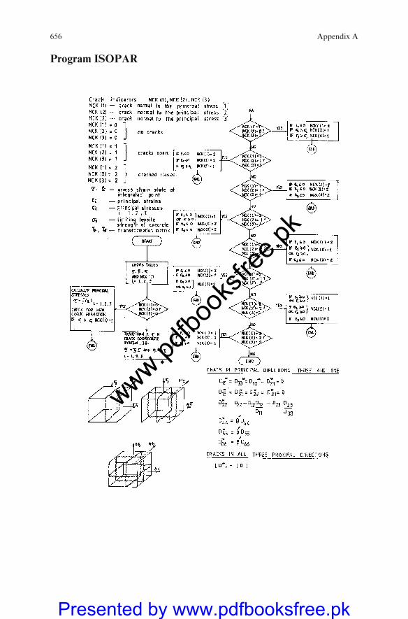
Program ISOPAR
656 Appendix A
www.pdfbo
oksfr
ee.pk
Presented by www.pdfbooksfree.pk
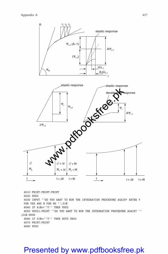
δ1
δtij
Rij
δtij + Δt
t + Δtl t + θt t + Δtl t + θt
δtij + θt
R1 + θtR1
+ Δt
δ
δ2 δ3R
K0
Ψi–l (A–1)
AΨi–l
AΨi–l
Ψi=lΨi
Ψi
(Ψi–l)
ΔUi–l
ΔΨi–l
AΔUi–l
elastic response
elastic response elastic response
decelerated response
t t
4510 PRINT:PRINT:PRINT4520 VDU34530 INPUT ‘‘DO YOU WANT TO RUN THE INTEGRATION PROCEDURE AGAIN? ENTER YFOR YES AND N FOR NO ’’;Z1$4540 IF A1$=‘‘Y’’ THEN VDU24550 VDU21:PRINT ‘‘DO YOU WANT TO RUN THE INTEGRATION PROCEDURE AGAIN? ’’
;Z1$:VDU64560 IF Z1$=‘‘Y’’ THEN GOTO 36504570 PRINT:PRINT4580 VDU3
=
=
Appendix A 657
www.pdfbo
oksfr
ee.pk
Presented by www.pdfbooksfree.pk

Ottosen Model
658 Appendix A
www.pdfbo
oksfr
ee.pk
Presented by www.pdfbooksfree.pk

Appendix A 659
www.pdfbo
oksfr
ee.pk
Presented by www.pdfbooksfree.pk

Main Program for Non-linear Analysis
660 Appendix A
www.pdfbo
oksfr
ee.pk
Presented by www.pdfbooksfree.pk

Appendix A 661
www.pdfbo
oksfr
ee.pk
Presented by www.pdfbooksfree.pk

662 Appendix A
www.pdfbo
oksfr
ee.pk
Presented by www.pdfbooksfree.pk

Appendix A 663
www.pdfbo
oksfr
ee.pk
Presented by www.pdfbooksfree.pk

664 Appendix A
www.pdfbo
oksfr
ee.pk
Presented by www.pdfbooksfree.pk

Appendix A 665
www.pdfbo
oksfr
ee.pk
Presented by www.pdfbooksfree.pk

666 Appendix A
www.pdfbo
oksfr
ee.pk
Presented by www.pdfbooksfree.pk

Appendix A 667
www.pdfbo
oksfr
ee.pk
Presented by www.pdfbooksfree.pk

668 Appendix A
www.pdfbo
oksfr
ee.pk
Presented by www.pdfbooksfree.pk

Appendix A 669
www.pdfbo
oksfr
ee.pk
Presented by www.pdfbooksfree.pk

670 Appendix A
www.pdfbo
oksfr
ee.pk
Presented by www.pdfbooksfree.pk

Appendix A 671
www.pdfbo
oksfr
ee.pk
Presented by www.pdfbooksfree.pk

672 Appendix A
www.pdfbo
oksfr
ee.pk
Presented by www.pdfbooksfree.pk

Appendix A 673
www.pdfbo
oksfr
ee.pk
Presented by www.pdfbooksfree.pk

674 Appendix A
www.pdfbo
oksfr
ee.pk
Presented by www.pdfbooksfree.pk

Appendix A 675
www.pdfbo
oksfr
ee.pk
Presented by www.pdfbooksfree.pk

676 Appendix A
www.pdfbo
oksfr
ee.pk
Presented by www.pdfbooksfree.pk

Appendix A 677
www.pdfbo
oksfr
ee.pk
Presented by www.pdfbooksfree.pk

678 Appendix A
www.pdfbo
oksfr
ee.pk
Presented by www.pdfbooksfree.pk

Appendix A 679
www.pdfbo
oksfr
ee.pk
Presented by www.pdfbooksfree.pk

680 Appendix A
www.pdfbo
oksfr
ee.pk
Presented by www.pdfbooksfree.pk

Appendix A 681
www.pdfbo
oksfr
ee.pk
Presented by www.pdfbooksfree.pk

682 Appendix A
www.pdfbo
oksfr
ee.pk
Presented by www.pdfbooksfree.pk

Appendix A 683
www.pdfbo
oksfr
ee.pk
Presented by www.pdfbooksfree.pk

684 Appendix A
www.pdfbo
oksfr
ee.pk
Presented by www.pdfbooksfree.pk

Appendix A 685
www.pdfbo
oksfr
ee.pk
Presented by www.pdfbooksfree.pk

686 Appendix A
www.pdfbo
oksfr
ee.pk
Presented by www.pdfbooksfree.pk

Appendix A 687
www.pdfbo
oksfr
ee.pk
Presented by www.pdfbooksfree.pk

688 Appendix A
www.pdfbo
oksfr
ee.pk
Presented by www.pdfbooksfree.pk

Appendix A 689
www.pdfbo
oksfr
ee.pk
Presented by www.pdfbooksfree.pk

690 Appendix A
www.pdfbo
oksfr
ee.pk
Presented by www.pdfbooksfree.pk

Appendix A 691
www.pdfbo
oksfr
ee.pk
Presented by www.pdfbooksfree.pk
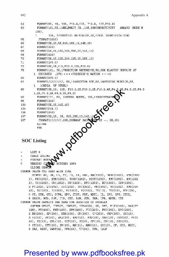
SOC Listing
692 Appendix A
www.pdfbo
oksfr
ee.pk
Presented by www.pdfbooksfree.pk

Appendix A 693
www.pdfbo
oksfr
ee.pk
Presented by www.pdfbooksfree.pk

694 Appendix A
www.pdfbo
oksfr
ee.pk
Presented by www.pdfbooksfree.pk

Appendix A 695
www.pdfbo
oksfr
ee.pk
Presented by www.pdfbooksfree.pk

696 Appendix A
www.pdfbo
oksfr
ee.pk
Presented by www.pdfbooksfree.pk

Appendix A 697
www.pdfbo
oksfr
ee.pk
Presented by www.pdfbooksfree.pk

698 Appendix A
www.pdfbo
oksfr
ee.pk
Presented by www.pdfbooksfree.pk

Appendix A 699
www.pdfbo
oksfr
ee.pk
Presented by www.pdfbooksfree.pk

700 Appendix A
www.pdfbo
oksfr
ee.pk
Presented by www.pdfbooksfree.pk

Appendix A 701
www.pdfbo
oksfr
ee.pk
Presented by www.pdfbooksfree.pk

702 Appendix A
www.pdfbo
oksfr
ee.pk
Presented by www.pdfbooksfree.pk

Appendix A 703
www.pdfbo
oksfr
ee.pk
Presented by www.pdfbooksfree.pk

704 Appendix A
www.pdfbo
oksfr
ee.pk
Presented by www.pdfbooksfree.pk

Appendix B
KOBE (Japan) Earthquake Versus Kashmir
(Pakistan) Earthquake
B.1. KOBE Earthquake versus Kashmir Earthquake
The summary of the Japanmeteorological Agency (JMA) has produced intensity
scale and range exists from 0 to 7.Mostly the areas come under disastrous (No. 6)
to very disastrous (No.7). Number 7 where collapse of more than 30 % of
wooden houses falling of objects, wavy deformation observed in horizon. The
Kashmir Earthquake was similar. Despite all these the brick houses together with
stoney ones, collapse like house of card. The Kobe Earthquake is known also as
Hyogo-KenManbu.Although various spring dampers were used. InKashmir no
such things existed. The damage could have been more, had Kashmir not having
stoney mountains or it had plane areas like KOBE. Based on modified Marcalli
(MM) of XII, and JMA 7, the positional scale of KOBE lies between them. The
disaster level in Azad Kashmir was much more it did not have modern construc-
tion of houses, roads and amenities. Many thousands of human beings were
carelessly killed or mammed in Kashmir since it did not have plane area to have
access to when compared with that of KOBE.
B.1 Data comparison
SerialNumber KOBE Kashmir
(1) ML = Magnitude = 7.6 onRichter Scale
$ Magnitude=7.6 on RichterScale
(2) Hypo-depth=10 Km $ Hypo-depth=16 km
(3) MW =Moment Magnitude = 6.9 $ 7.2
(4) MS = Surface Magnitude = 6.9 $ 7.2
(5) Epicentre Location = 34.527 N,135.005E
$ 40.35 N
123.00(6) Fault line 50 km long SE (affecting
small areas)$ 100 km long NS (affecting
large areas)
(7) Accumulated stress Equivalent to‘‘2 No’’ Earthquake ML = 8.5or larger
$ Accumulated stressEquivalent ‘‘4 No’’Earthquake ML = 8.5or larger
Acceleration $ Velocity
(8) (Max) (cm/s/s) Component (Max) (CMax) (cm/s)
N-S EW UD $ N-S EW UD
818.0 617.3 332.2 $ 55.1 344 cm/s 20.6 cm/s
www.pdfbo
oksfr
ee.pk
Presented by www.pdfbooksfree.pk

B.1 (continued)
SerialNumber KOBE Kashmir
(9) Energy $ Energy
More Eg. Less than Kashmir.Acceleration greater or lesserless energy. Separation time lessbetween horizontal wave andslowing moving surface wave islonger and hence less impactand less destructive
$ More ES, greater from 16 kmdepth. More energy Es
transferred to the surface.Separation time is sharper.More impact, moredestruction
(10) Vertical component ofacceleration=21%
$ Vertical component ofacceleration 30%
(11) Peak ground acceleration from site within 10 km from zone of intense destruction,the fault zone of KOBE Earthquake
Kobe Motoyama
PGA (g) = 0.79
$ Kashmir
Muzzafar AbadPGA (g) = 0.83
* Estimate distance from faultline = 1 km
* Estimate 2 km distance
Kobe University Border Area
PGA(g) = 0.31 PGA (g) = 0.32 to 0.33
* Distance=3 km *Distance=3 km
* Distance from site within 10 kmof the zone fo destruction.
706 Appendix B
www.pdfbo
oksfr
ee.pk
Presented by www.pdfbooksfree.pk