1 

 

Citation: Hirt, C. and M. Rexer (2015), Earth2014: 1 arc‐min shape, topography, bedrock and ice‐sheet models – 

available as gridded data and degree‐10,800 spherical harmonics, International Journal of Applied Earth 

Observation and Geoinformation 39, 103‐112, doi:10.1016/j.jag.2015.03.001. 

Earth2014:  1  arc‐min  shape,  topography,  bedrock  and  ice‐sheet models  – 

available as gridded data and degree‐10,800 spherical harmonics 

Christian Hirt1,2 

Email: c.hirt@curtin.edu.au  

Moritz Rexer2 

Email: m.rexer@tum.de 

1  Western  Australian  Geodesy  Group  &  The  Institute  for  Geoscience  Research  &  Department  of 

Spatial Sciences, Curtin University Perth, WA, Australia 

2  Institute  for  Advanced  Study  &  Institute  for  Astronomical  and  Physical  Geodesy,  TU  Munich, 

Germany 

Highlights 

Earth2014 topography, ice, bedrock and shape models constructed at 1arcmin resolution 

Earth2014 relies on SRTM30_PLUS, SRTM V4.1, Bedmap2 and Greenland Bed Topography v3 

Earth2014 suite comprises five topography and shape grid layers, freely available  

Models expanded into degree 10,800 spherical harmonic series for spectral modelling 

Analyses of model characteristics, power spectra, and external comparisons provided 

Abstract  

Since the release of the ETOPO1 global Earth topography model through the US NOAA in 2009, new 

or  significantly  improved  topographic data  sets have become available over Antarctica, Greenland 

and parts of  the oceans.   Here we present a suite of new 1 arc‐min models of Earth’s topography, 

bedrock and ice‐sheets constructed as a composite from up‐to‐date topography models: Earth2014. 

Our model suite relies on SRTM30_PLUS v9 bathymetry for the base  layer, merged with SRTM v4.1 

topography  over  the  continents,  Bedmap2  over  Antarctica  and  the  new  Greenland  Bedrock 

Topography  (GBT  v3). As  such, Earth2014 provides  substantially  improved  information of bedrock 

and  topography over Earth’s major  ice  sheets,  and more  recent bathymetric depth data over  the 

oceans, all merged into readily usable global grids. To satisfy multiple applications of global elevation 

data, Earth2014 provides different representations of Earth’s relief. These are grids of (1) the physical 

surface, (2) bedrock (Earth’s relief without water and ice masses), (3) bedrock and ice (Earth without 

water masses),  (4)  ice  sheet  thicknesses,  (5)  rock‐equivalent  topography  (ice  and  water masses 

condensed  to  layers  of  rock)  as mass  representation.  These models  have  been  transformed  into 

ultra‐high degree  spherical harmonics,  yielding degree  10,800  series  expansions of  the  Earth2014 

grids as  input  for spectral modelling  techniques. As  further variants, planetary shape models were 

constructed, providing distances between relief points and  the geocenter. The paper describes  the 

input  data  sets,  the  development  procedures  applied,  the  resulting  gridded  and  spectral 

  2 

 

representations of Earth2014, external  validation  results  and possible  applications. The Earth2014 

model suite is freely available via http://ddfe.curtin.edu.au/models/Earth2014/ 

Key  words:  Earth2014,  topography,  bathymetry,  bedrock,  ice  sheets,  planetary  shape,  spherical 

harmonics, composite model 

1. Introduction 

Detailed  global  information  on  Earth’s  relief  –  encompassing  land  topography,  ocean  and  lake 

bathymetry and ice information – is essential for numerous geoscience applications. Examples are as 

diverse as modelling of  the Earth’s gravity  field  (Balmino et al. 2012, Hirt et al. 2013), occurrence 

analysis  of  submarine  canyons  (Harris  and Whiteway  2011),  and  of  seamounts  (Sandwell  et  al. 

2014a), ocean wave refraction studies  (Li et al. 2010), visualisation of relief  for geophysical studies 

(Tape  et  al.  2010),  statistical  relief  analysis  in  terms of hypsometric  curves  and  terrain  roughness 

(Melosh 2011), construction of crustal models (Molinari and Morelli 2011, Reguzzoni and Sampietro 

2015) and aid in analysis of large‐scale geological formation (Stampfli et al. 2013). 

In  the presence of ocean water and  ice  coverage,  it  is not possible  to obtain global  relief models 

based on a  single homogeneous data  source or observation  technique  (e.g.,  remote  sensing  from 

space).  High‐resolution  digital  terrain  models,  e.g.,  from  the  Shuttle  Radar  Topography  Mission 

(SRTM, e.g., Rabus et al. 2003) or Advanced Spaceborne Thermal Emission and Reflection Radiometer 

(ASTER, e.g., Tachikawa et al. 2011) mission, provide elevations over  land areas only, while digital 

bathymetry models – from altimetry, echo soundings, or combinations thereof – aim to describe the 

seafloor  or  lake  bottom  topography  (Becker  et  al.  2009).  Bedrock  elevations  (i.e.,  sub‐ice‐

topography) are often obtained from airborne radar measurements (Fretwell et al. 2013). 

Earth relief models with global coverage are thus obtained as composites constructed from different 

data sources over land, water and ice‐covered areas. Notable examples of composite models are (1) 

the 1  arc‐min  global  ETOPO1  (by United  States National Oceanic  and Atmospheric Administration 

NOAA,  Amante  and  Eakins  2009),  which  combines  ice  thickness  data  with  bathymetry  and 

topography elsewhere, and (2) the 30 arc‐sec SRTM30_PLUS (by Scripps Institution of Oceanography, 

California, USA, Becker et al. 2009) data set as a global merger of altimetry‐derived and ship‐track 

bathymetry  and  SRTM  topography.  SRTM30_PLUS  is  provided  as  one‐layer  representation, while 

ETOPO1 comprises two layers of information (bedrock and ice surface heights).  

Recently, significantly improved bed, surface and ice thickness data sets have become available with 

the  Bedmap2  (Fretwell  et  al.  2013)  data  compilation  over  Antarctica,  and  the  GBT  bedrock 

topography  (Bamber et al. 2013) over Greenland. Further, the SRTM30_PLUS bathymetry has been 

updated about annually with new depth soundings and/or improved depth estimates from altimetry 

(Sandwell et al. 2014b). As a result, ETOPO1 is based to some extent on now‐outdated data sets over 

the oceans  and  ice‐covered  regions, while  SRTM30_PLUS does not  yet  incorporate  recent  surface 

height  data  over  the  ice‐sheets.  However,  for many  current  applications  of  global  relief  data,  a 

merged data set representing Earth’s surface, ice and bedrock based on recent data would be useful. 

This  paper  presents  of  suite  of  new  models  of  Earth’s  topography,  bedrock  and  ice‐sheets 

constructed  as  a  composite  from  up‐to‐date  topography models:  Earth2014.  To  satisfy multiple 

applications of global relief data, Earth2014 provides readily usable grids of (1) the physical surface 

SUR, (2) bedrock BED (Earth’s relief without water and ice masses), (3) topography, bedrock and ice 

  3 

 

TBI (representing Earth without water masses), (4) ice sheet thicknesses ICE, and (5) rock‐equivalent 

topography RET  (ice and water masses condensed to  layers of rock) as mass representation. These 

models  have  been  expanded  into  ultra‐high  degree  spherical  harmonics,  yielding  degree  10,800 

series expansions of the Earth2014 grids as  input for spectral modelling techniques frequently used 

in  geodesy  and  geophysics.  As  further  variants,  planetary  shape models  have  been  constructed, 

providing distances between  relief points  and  the  geocenter. While  the  topography models  (SUR, 

BED,  TBI,  and RET) use  the mean  sea  level  as  vertical datum,  the  vertical  reference of  the  shape 

models is the geocenter. 

Earth2014 relies on SRTM30_PLUS v9 bathymetry as base layer, merged with SRTM v4.1 topography 

over the continents, Bedmap2 over Antarctica and the Greenland Bedrock Topography  (GBT v3) as 

input data (Section 2). Section 3 summarizes the data processing applied to yield the Earth2014 grids. 

Section 4 characterizes the new relief models, e.g., in terms of geo‐statistics, hypsometric curves, and 

degree variance power spectra, and provides selected 3D visualizations. The Earth2014 global grids 

are compared against ETOPO1 and SRTM30_PLUS (Section 5), before outlining some applications and 

drawing conclusions in Section 6.  

2. Input data 

The Earth2014 suite of global relief and topography models is based on four input data sets,  

(i) SRTM30_PLUS (Becker et al. 2009) v9 (Dec 2013) bathymetry and topography model,  

(ii) the SRTM V4.1 topography (Jarvis et al. 2008) over all land areas between 60° latitude,  

(iii) Bedmap2  (Fretwell  et  al.  2013)  bedrock,  bathymetry  and  ice  thickness  data  over 

Antarctica, 

(iv) and the Greenland Bedrock Topography (GBT v3, Bamber et al. 2013, Bamber 2014, pers. 

comm.).  

Fig.  1  shows  the  spatial  coverage  of  the  four  input  data  sources.  The  30  arc‐sec  SRTM30_PLUS 

bathymetry  and  topography model  (Becker  et  al.  2009)  serves  as  the  background  layer  for  Earth 

2014. Over  land areas, SRTM30_PLUS relies on GTOPO30 topography North of 60°  latitude (Arctic),  

ICESat  ice  surface  heights  (DiMarzio  et  al.  2007),  and  SRTM30  topography  elsewhere.  Over  the 

oceans,  SRTM30_PLUS  v9  provides  depth  information  based  on  inverted  altimetry  gravity  data 

(including  new mission  data  such  as  Cryosat‐2,  Jason‐1  and  Envisat),  and  a  compilation  of  ~300 

million  soundings  (ship‐track  data). According  to  Becker  et  al.  (2009),  “approximately  10%  of  the 

seafloor  has  been mapped  by  echo  sounders  at  a  1‐minute  resolution”  only.  The  SRTM30_PLUS 

model  also  contains  bathymetric  depth  information  for  Earth’s  major  inland  lakes  (Superior, 

Michigan, Huron, Erie, Ontario and Baikal) and the Caspian Sea, which is the relevant data source for 

Earth2014 inland bathymetry. 

Over all  (dry)  land areas within 60° North and  South  latitude,  the 7.5 arc‐sec  (~250 m)  resolution 

SRTM V4.1  topography model  (Jarvis  et  al. 2008)  is  the  source  for  Earth2014.  SRTM4.1  is  a post‐

processed  SRTM  release  where  voids  were  filled  using  advanced  interpolation  techniques  and 

auxiliary data sets as described in Reuter et al. (2007).   

  4 

 

The 2013 Bedmap2  (Fretwell et al. 2013) data  set encompasses 1‐km  resolution grids of bedrock, 

surface topography, ice‐shelf and ice‐sheet thicknesses (mostly from airborne radar) and bathymetric 

depths over  the Antarctic  region.  Importantly,  the Bedmap2 collection  incorporates a multitude of 

new  ice thickness and surface elevation data sets originating from surveys conducted or completed 

since the release of the predecessor Bedmap1 (Lythe et al. 2001).   

The Bedmap2 grids substantially improve over earlier Bedmap1 data compilations over Antarctica, as 

is evident e.g., from independent comparisons against gravimetry (Hirt 2014). Differences in bedrock 

elevations  between  Bedmap2  and  Bedmap1  are  at  the  level  of  several  100  m  (up  to  1‐2  km 

maximum), where new ice thickness data has become available (Fretwell et al. 2013, Fig 13 ibid). This 

is  important  for  comparisons  with  ETOPO1  which  is  based  on  Bedmap1  bedrock  (Section  5). 

Bedmap2  surface heights only marginally  rely on  the 2007  ICESat measurements, and  instead are 

based on a combination of several newer digital elevation models (e.g., Bamber et al. 2009, Cook et 

al.  2012)    “to  exploit  the  strengths  of  each”  (Fretwell  et  al.  2013,  p381).  This  is  relevant  for 

comparisons  of  Earth2014  surface  heights with  SRTM30_PLUS  over  Antarctica  (from  2007  ICESat 

data), and with ETOPO1 (taken from the Radarsat Antarctic Mapping Project topography v2 released 

back in 2001) in Section 5. Over Greenland the GBT v3 (Bamber et al. 2013) product is conceptually 

similar  to  Bedmap2,  in  that,  it  provides  grids  of  ice‐thicknesses,  surface  topography  and 

bedrock/bathymetry based on newly compiled data at 1 km resolution.  

3 Processing 

3.1 Grid merging 

Relief  information from the four data sets was merged by using SRTM30_PLUS as “base  layer”, and 

subsequently  inserting  the SRTM V4.1, Greenland and Antarctica data sets.  In a  first step, artifacts 

detected at about ~3,000 cells in the V4.1 250 m release over parts of Asia were removed and fixed 

as described in Hirt et al. (2014). Second, SRTM30_PLUS and SRTM V4.1 elevations were combined at 

the highest possible  resolution of 7.5 arc‐sec by  (i) up‐sampling SRTM30_PLUS by a  factor 4 using 

bicubic  interpolation, and  (ii)  inserting SRTM V4.1 elevations where  land areas are  flagged through 

the SRTM sea‐mask (V4.1). 

 Third, inland bathymetry (Great Lakes, Baikal, Caspian Sea) was taken into account. Given the input 

data  set  “SRTM30_PLUS v9”  is not accompanied by a mask grid  that would allow  identification of 

inland bathymetry, a procedure to identify inland lake bathymetry had to be developed and applied. 

We  identified  inland  bathymetry  as  regions  of  certain  extent  (>  2000  cells)  with  bedrock 

(SRTM30_PLUS)  located at  least 5 metres below  the surface  topography  (SRTM V41).   Because  the 

SRTM V4.1 and SRTM30_PLUS  information  is not  identical over dry  land (among other effects there 

are oscillating positive and negative discrepancies reflecting the resolution effect of 7.5 arc‐sec vs. 30 

arc‐sec, and thus additional high‐frequency features in the V4.1 data set) it was necessary to impose 

a minimum size for regions considered as inland lakes. While the criterion applied is pragmatic in our 

case,  it  cannot  completely  extract  the  lake margins  along  the  inland  lake  coastlines  (e.g.,  shallow 

depths were neglected by our  criterion).  For  the  lake  extraction we  applied  region  growing  (e.g., 

Adams and Bischof 1994), a segmentation technique often used  in digital  image analysis to extract 

areas of similar characteristics. As the basic idea of region growing as done here, adjoining cells with 

systematically positive elevation differences SRTM V4.1 minus SRTM30_PLUS are grouped together 

through iterative search, yielding regions (segments) considered as lake areas. 

  5 

 

 

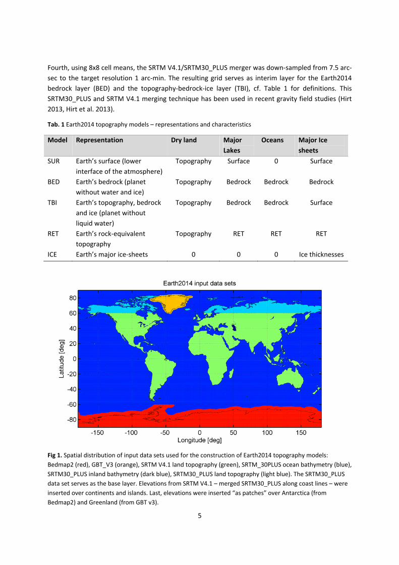
Fourth, using 8x8 cell means, the SRTM V4.1/SRTM30_PLUS merger was down‐sampled from 7.5 arc‐

sec  to  the  target  resolution 1 arc‐min. The  resulting grid serves as  interim  layer  for  the Earth2014 

bedrock  layer  (BED)  and  the  topography‐bedrock‐ice  layer  (TBI),  cf.  Table  1  for  definitions.  This 

SRTM30_PLUS and SRTM V4.1 merging technique has been used  in recent gravity field studies (Hirt 

2013, Hirt et al. 2013). 

Tab. 1 Earth2014 topography models – representations and characteristics 

Model  Representation  Dry land  Major 

Lakes 

Oceans  Major Ice 

sheets 

SUR  Earth’s surface (lower 

interface of the atmosphere) 

Topography  Surface  0  Surface 

BED  Earth’s bedrock (planet 

without water and ice) 

Topography  Bedrock  Bedrock  Bedrock 

TBI  Earth’s topography, bedrock 

and ice (planet without 

liquid water) 

Topography  Bedrock  Bedrock  Surface 

RET  Earth’s rock‐equivalent 

topography 

Topography  RET  RET  RET 

ICE  Earth’s major ice‐sheets  0  0  0  Ice thicknesses 

 

 

Fig 1. Spatial distribution of input data sets used for the construction of Earth2014 topography models: 

Bedmap2 (red), GBT_V3 (orange), SRTM V4.1 land topography (green), SRTM_30PLUS ocean bathymetry (blue), 

SRTM30_PLUS inland bathymetry (dark blue), SRTM30_PLUS land topography (light blue). The SRTM30_PLUS 

data set serves as the base layer. Elevations from SRTM V4.1 – merged SRTM30_PLUS along coast lines – were 

inserted over continents and islands. Last, elevations were inserted “as patches” over Antarctica (from 

Bedmap2) and Greenland (from GBT v3).

  6 

 

 

Fig 2. Spatial distribution of main types of terrain in Earth2014. Ice‐free land above mean sea level MSL (green) 

and below MSL (red), ice‐covered land (white), ice‐covered water (dark blue), oceans (blue), inland water 

bodies (dark red). 

The  described  procedure was  repeated  to  yield  global  1  arc‐min  grids  of  Earth’s  surface  SUR  (by 

setting ocean depths  to  0,  and  replacing  inland bathymetry with  lake  surface heights  from  SRTM 

v4.1), and of Earth’s rock‐eqivalent topography (RET), which is a dedicated Earth2014 layer for mass 

modelling and gravity applications. RET  is a model  that  represents  ice and water masses as mass‐

equivalent layers of rock, added to the Earth2014 BED bedrock layer (cf. appendix A for procedures). 

While the SRTM data sets and their merger are given  in terms of global geodetic  latitude‐longitude 

grids, both the Bedmap2 and GBT v3 data grids are  in polar stereographic (PS) projection, requiring 

coordinate transformation from PS to geodetic coordinates (and thus interpolation). Bedrock, surface 

and RET heights were extracted or computed at 1 km resolution in PS projection before transforming 

to geodetic coordinates. As  last step, the Bedmap2 and GBT v3 patches (BED, SUR, RET and ICE  ice‐

sheet  thicknesses) were  inserted  into  the SRTM‐merger over  the areas  shown  in Fig. 1, giving  the 

Earth2014 global grids at 1 arc‐min resolution.  

It  is  important to note that the Bedmap2 data ‘patched’  into the SRTM V4.1/SRTM30_PLUS merger 

covers  continental Antarctica and a ~400  km margin  (buffer) over  the adjoining oceans  (Fig. 1)  in 

order to preserve the self‐consistency of the Bedmap2 products over  land and sea. Along the same 

lines, a ~200km ocean zone surrounding Greenland is taken from GBT v3 and included in Earth 2014. 

The margin sizes were chosen such that  inconsistencies between the SRTM30_PLUS and Bedmap2, 

and  SRTM30_PLUS  and GBT  v3  bathymetry were  kept  reasonably  small.  Along  the merging  lines 

(red/blue  and  orange/blue  boundaries  in  Fig.  1),  bathymetry  differences  of  ‐1033/+1017/101 m 

(min/max/  root‐mean‐square) were  observed w.r.t.  Bedmap2,  and  ‐464/580/54 m w.r.t. GBT  v3, 

reflecting uncertainties  in current bathymetry data.  In  future versions of  the Earth relief models, a 

tapered transition between the data sets could be considered. Not using a tapered transition creates 

  7 

 

artificial features along the merging lines (cf. Fig. 1), which should not be misinterpreted as steps in 

the seafloor topography. 

3.2. Shape modelling 

For  geophysical  applications  and  geo‐visualisation,  shape  models  were  derived  for  the  various 

Earth2014  topography models. While  the previously described  relief models provide elevations of 

the topography or bedrock with respect to the mean sea level, shape models represent the geometry 

of  the  planet  via  the  planetary  radius  (i.e.,  distances  Pr   between  the  geocenter  and  the  surface 

points).   As such, relief and shape models differ by the sum of (a) the ellipsoidal radius, and (b) the 

geoid height, with the  latter being an approximation of the separation between the mean sea  level 

and  the  ellipsoid  surface.  Following  this  definition,  radii  Pr   of  the  Earth2014  shape models were 

constructed  as  sum  of  ellipsoidal  radii  Er ,  geoid  undulations  N   and  relief  heights  PH (bedrock, 

surface or RET heights, depending on the model) 

P E Pr r N H                   (1) 

where ellipsoidal radii are computed via (equation after Claessens 2006) 

2 2 2

2 2

1 2 sin

1 sinE

e er a

e

              (2) 

with  geodetic latitude,  a semi‐major axis, and  b semi‐minor axis of the GRS80 reference ellipsoid 

(Moritz 2000) and  

2 22

2

a be

a

                     (3) 

the  first  numerical  eccentricity  squared.  Geoid  undulations  N   were  obtained  from  the  EGM96 

geopotential model (Lemoine et al. 1998)  in spectral band of harmonic degrees 2 to 360. EGM96  is 

used  here  as model  of  the  geoid  because  EGM96  provided  the  vertical  reference  for  the  SRTM 

elevation model. We note that the choice of the geoid model  is not too much a concern for global 

relief modelling, given the differences between present geoid models are mostly at or  less the 1m‐

level. 

3.3 Transformation to ultra‐high degree spherical harmonics 

A convenient way to represent a global topography model is in terms of surface spherical harmonic 

coefficients  (SHCs),  see e.g. Balmino et al.  (2012) and Pavlis et  al.  (2012). By evaluating a  surface 

spherical harmonic expansion (SHE) of the discrete form (e.g., Claessens 2006) 

max

0

, ,n n

nm nmn m n

H T Y

               (4) 

with  the  fully normalized SHCs  nmT    of degree n and order m  (m<0:  sine associated; m≥0:  cosine 

associated), the elevation H of the topography model can be retrieved at any point on Earth, given by  

  8 

 

geocentric  latitude   and longitude  .  nmY  denote the spherical harmonic functions that evaluate 

the associated Legendre functions (ALFs) depending on the co‐latitude, and sine / cosine arguments 

depending on longitude. Variable  maxn   is the maximum degree of the model and defines the spatial 

resolution of the model. 

In order to generate the SHCs for the topography grids (from Section 3.1) we make use of a Gauss‐

Legendre  spherical  harmonic  analysis  (SHA)  procedure  (see  e.g.  Sneeuw  and  Bun,  1996).  We 

extended the SHTOOLS package v2.8 (Wieczorek, 2012) in order to achieve stability of the routines to 

ultra‐high degree. In the original form SHTOOLS v2.8 is restricted to spherical harmonic computations 

up  to  degree  ~2800,  due  to  the  numerical  instability  of  the  ALF  implementation  (Holmes  and 

Featherstone  2002). We modified  the  existing  ALF  computation method with  ALFs  based  on  the 

extended  range‐arithmetic  approach  (Fukushima  2012),  allowing  stable  computation  of  the 

associated Legendre polynomials up to arbitrary degree and order.  

In this work five sets of SHCs of maximum degree and order 10800, corresponding to the resolution 

of  the  topography  grids  (1  arc‐min),  are  computed  (cf.  Section  4.2). Closed  loop  tests with band‐

limited functions of degree 10800 show that the modified SHA procedure works satisfactorily, with 

maximum errors below 3 x 10‐6 m in the space domain. Note that the functions  ,H  described 

by  the  topography  grids  are  usually  not  band‐limited.  Therefore  the  topography  grids  cannot  be 

exactly represented by a SHE of degree N<. Tests that involve the entire workflow to generate the SHCs and a subsequent spherical harmonic synthesis show a global RMS (root mean square) below 9 

m  (maximum errors may exceed 100 m  in steep  terrain)  for  the chosen degree  maxn =10800.  If  full 

topographic  information  is sought, the data grids should be used  instead of the spherical harmonic 

representations.  

4. Results 

4.1 Spatial domain 

The main result of this work is the Earth2014 set of 1 arc‐min global grid layers which represent the 

physical surface (SUR), bedrock (BED), bedrock, land topography and  ice (TBI), ice sheet thicknesses 

(ICE), and  rock‐equivalent  topography  (RET, also denoted with RET2014  for  reasons of consistency 

for previous releases). The BED layer represents Earth’s relief without water and ice masses, and the 

TBI  layer  Earth’s  relief  without  ocean  and  lake  water masses,  they  thus  differ  by  the  ice  sheet 

thicknesses  (and  water  columns  below  ice  over  parts  of  Antarctica).  Table  1  summarizes  the 

differences between the five global Earth2014 grid layers which all provide in approximation physical 

heights (w.r.t mean sea level) of the relief. 

The five grids are self‐consistent in that, BED elevations are never larger than SUR or TBI, or RET, or 

TBI minus  ICE elevations,  ICE  is positive or zero anywhere on Earth, and TBI minus  ICE minus BED 

provides water column heights below  ice. Fig. 2  shows a global map of  the different  terrain  types 

(ice‐sheets,  ice‐shelves, dry  land above and below the mean sea  level, oceans and  lakes) extracted 

from the  input data sets and modelled  in Earth2014. Fig. 3 provides 3D visualisations of four Earth 

2014  topography  models,  illustrating  the  differences  between  the  SUR,  BED,  TBI  and  RET 

representations of Earth’s relief. 

  9 

 

 

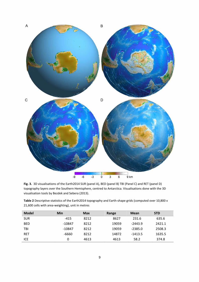
Fig. 3.  3D visualisations of the Earth2014 SUR (panel A), BED (panel B) TBI (Panel C) and RET (panel D) 

topography layers over the Southern Hemisphere, centred to Antarctica. Visualisations done with the 3D 

visualisation tools by Bezdek and Sebera (2013). 

Table 2 Descriptive statistics of the Earth2014 topography and Earth‐shape grids (computed over 10,800 x 

21,600 cells with area‐weighting), unit in metres 

Model  Min  Max  Range  Mean  STD 

SUR  ‐415   8212  8627     231.6     635.6 

BED  ‐10847   8212  19059   ‐2443.9    2421.1 

TBI  ‐10847   8212  19059   ‐2385.0    2508.3 

RET  ‐6660   8212  14872   ‐1413.5    1635.5 

ICE  0   4613  4613      58.2     374.8 

 

  10 

 

Table 2  reports  the descriptive  statistics of  the  Earth2014  grids, whereby  the mean  and  standard 

deviation (STD) take into account the area size of the individual grid cells to prevent overweighting of 

polar regions. The minimum and maximum values show that at 1 arc‐min grid resolution the actual 

relief  is  low‐pass  filtered,  so  cannot exactly  represent Mount Everest’s 8,848 m  summit and  the  ‐

10,911 m  depression  of  the Mariana  Trench.  The  STD  values  are  a measure  for  the  global  relief 

roughness of  the  Earth2014  grid  layers,  e.g.,  636 m  for  the physical  surface,  and  2421 m  for  the 

bedrock model. 

 

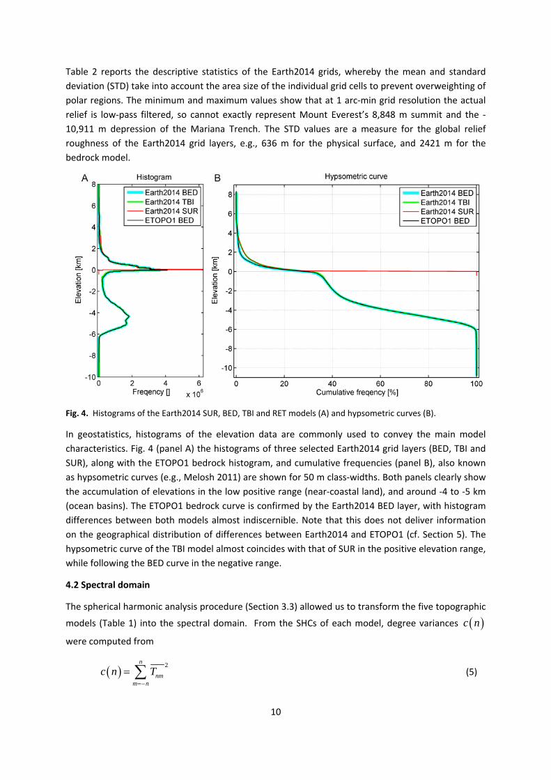
Fig. 4.  Histograms of the Earth2014 SUR, BED, TBI and RET models (A) and hypsometric curves (B).  

In  geostatistics,  histograms  of  the  elevation  data  are  commonly  used  to  convey  the main model 

characteristics. Fig. 4 (panel A) the histograms of three selected Earth2014 grid layers (BED, TBI and 

SUR), along with the ETOPO1 bedrock histogram, and cumulative frequencies (panel B), also known 

as hypsometric curves (e.g., Melosh 2011) are shown for 50 m class‐widths. Both panels clearly show 

the accumulation of elevations in the low positive range (near‐coastal land), and around ‐4 to ‐5 km 

(ocean basins). The ETOPO1 bedrock curve is confirmed by the Earth2014 BED layer, with histogram 

differences between both models almost  indiscernible. Note  that  this does not deliver  information 

on the geographical distribution of differences between Earth2014 and ETOPO1 (cf. Section 5). The 

hypsometric curve of the TBI model almost coincides with that of SUR in the positive elevation range, 

while following the BED curve in the negative range. 

4.2 Spectral domain 

The spherical harmonic analysis procedure (Section 3.3) allowed us to transform the five topographic 

models  (Table 1)  into  the spectral domain.   From  the SHCs of each model, degree variances  c n  

were computed from 

2n

nmm n

c n T

                  (5) 

  11 

 

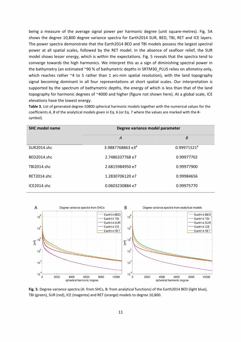
being  a measure  of  the  average  signal  power  per  harmonic  degree  (unit  square‐metres).  Fig.  5A 

shows the degree 10,800 degree variance spectra for Earth2014 SUR, BED, TBI, RET and  ICE  layers. 

The power spectra demonstrate that the Earth2014 BED and TBI models possess the largest spectral 

power  at  all  spatial  scales,  followed by  the RET model.  In  the  absence of  seafloor  relief,  the  SUR 

model shows  lesser energy, which  is within the expectations. Fig. 5 reveals that the spectra tend to 

converge  towards  the high harmonics. We  interpret  this as a sign of diminishing spectral power  in 

the bathymetry (an estimated ~90 % of bathymetric depths in SRTM30_PLUS relies on altimetry‐only, 

which  reaches  rather  ~4  to  5  rather  than  1  arc‐min  spatial  resolution), with  the  land  topography 

signal becoming dominant  in  all  four  representations  at  short  spatial  scales. Our  interpretation  is 

supported by the spectrum of bathymetric depths, the energy of which  is  less than that of the  land 

topography for harmonic degrees of ~4000 and higher (figure not shown here). At a global scale, ICE 

elevations have the lowest energy. 

Table 3. List of generated degree‐10800 spherical harmonic models together with the numerical values for the 

coefficients A, B of the analytical models given in Eq. 6 (or Eq. 7 where the values are marked with the #‐

symbol).  

SHC model name  Degree variance model parameter 

A  B 

SUR2014.shc  3.9887768863 e3# 0.99971521# 

BED2014.shc  2.7486337768 e7  0.99977702 

TBI2014.shc  2.6815984950 e7  0.99977900 

RET2014.shc  1.2830706120 e7  0.99984656 

ICE2014.shc  0.0603230884 e7  0.99975770 

 

 

 

Fig. 5. Degree‐variance spectra (A: from SHCs, B: from analytical functions) of the Earth2014 BED (light blue), 

TBI (green), SUR (red), ICE (magenta) and RET (orange) models to degree 10,800. 

 

  12 

 

Overall,  the curves  in Fig. 5  illustrate  the decay of  the  topographic  relief with  increasing harmonic 

degree, here for the first time for five representations complete to degree 10,800. We acknowledge 

work by Balmino et al. (2012) who have provided degree 10,800 spectra for the ETOPO1 topography 

(one layer only).   

Further, we have approximated the degree variances   c n  by analytical models of the type 

, 3

1 2

nA Bd n n

n n

               (6) 

or 

, 2

1

nA Bd n n

n

                 (7) 

where A and B are the model‐specific parameters, estimated through a  least‐squares fit for each of 

the  five  topography model  spectra. The numerical  values  for  the A, B  coefficients are  reported  in 

Table 3. Our analytical degree variance model  d n   is well suited to model the spectra of most of 

the topography models. The spectrum of the SUR model is the only exception, here Eq. (6) does not 

well approximate  the  spectra. Therefore  the analytical model  d n   (Eq. 7) has been used  in  this 

case (the spectrum at low degrees is still underestimated, but the approximation delivers a good fit 

for n>1000). 

5. Comparison with ETOPO1 and SRTM30_PLUS 

This  section  reports  results  from  comparisons  between  selected  Earth2014  grid  layers  against 

ETOPO1  and  SRTM30_PLUS  v9.  Earth2014  is  formally  independent  from  ETOPO1. However,  some 

indirect  relationship  exists  between  the models  because  of  both  using  land  topography  from  the 

SRTM mission.  

Fig. 6 (panel A) shows the differences between the bedrock layers of Earth2014 and ETOPO1 at 1 arc‐

min resolution. While there is generally good agreement (often at the level of few metres) over most 

ice‐free and dry  land areas, notable discrepancies exist over  the oceans, with amplitudes of  some 

100 m to km. Given that ETOPO1 is based on a 2008 measured/estimated 2 arc‐min bathymetry grid 

by  Scripps  Institution  of  Oceanography  (Amante  and  Eakins  2009,  p9),  we  interpret  these 

discrepancies (somewhat cautiously) as improvements of the seafloor topography in SRTM30_PLUS, 

and thus in Earth2014. Differences over mountainous regions are likely to reflect different SRTM hole 

filling procedures (e.g., over Himalayas), inland bathymetry modelled in Earth2014 (e.g., Lake Baikal), 

but not in ETOPO1, and conversely (e.g., Lake Victoria, modelled in ETOPO1 only).  

Further  very  pronounced  differences  of  several  100 m  amplitude  exist  over  Antarctica  (Fig.  7A), 

which unambiguously  reflect  the  improvements  from  the 2001 Bedmap1  (used  in ETOPO1)  to  the 

2013 Bedmap2 data set  (used  in Earth2014), also see Fretwell et al.  (2013, p389). Along  the same 

lines, differences with somewhat  less pronounced amplitudes over Greenland can be considered to 

reflect errors in the 2001 5km‐resolution Greenland bedrock data by the National Snow and Ice Data 

Centre (Bamber et al. 2013, p506) that was used in ETOPO1 (Amante and Eakins 2009, p11). 

  13 

 

 

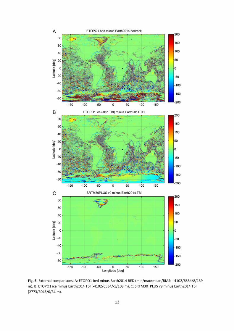
Fig. 6. External comparisons. A: ETOPO1 bed minus Earth2014 BED (min/max/mean/RMS: ‐ 4102/6534/8/139 

m), B: ETOPO1 ice minus Earth2014 TBI (‐4102/6534/‐1/108 m), C: SRTM30_PLUS v9 minus Earth2014 TBI 

(2773/3045/0/34 m). 

  14 

 

Fig.  6  (panel  B)  displays  the  differences  between  the  Earth2014  TBI  and  the  ETOPO  ice  product, 

which  equally  provide  topographic  elevations  over  land,  ice  surface  heights  over  Antarctica  and 

Greenland, and bathymetry elsewhere. The comparisons in Figs. 6A and 6B thus only differ over the 

ice‐sheets. ETOPO1 and Earth2014 ice surface heights are close together over Greenland (10m level 

over  large parts of central Greenland), while often ~50‐100 m apart over Antarctica. This  suggests 

larger changes in the underlying ice surface data sets over Antarctica than Greenland. 

The comparison between SRTM30_PLUS and Earth2014 TBI (Fig. 6C) has mostly internal character. It 

verifies the Earth2014 processing (mostly zero or m‐level differences) over the oceans. Some  larger 

differences exist over mountain areas  (indicating different hole‐filling procedures between SRTM30 

and SRTM V4.1). Over Antarctica and Greenland, and surrounding waters, the comparison  in Fig 6C 

has  external  character.  The  largely  green  areas  over  continental  Antarctica  suggest  that  the  ice 

surface heights are similar in both products (around the South Pole, however, the 2007 ICESat model 

and thus SRTM30_PLUS deviates by ~20 m from the newer data used in Earth2014). 

Notable differences  (100s of m amplitude) between Earth2014 and SRTM30_PLUS bathymetry are 

visible along the Antarctic and Greenland coastlines, where Earth2014 is based on the Bedmap2‐ and 

GBT v3‐provided bathymetric depth  information (Fig. 6C), also see Sect. 3.1.  In the absence of true 

reference data, we cannot attribute  the differences  to a specific model. Fig. 6C  thus  illustrates  the 

differences between the underlying data bases, and probably indicates the error level of up‐to‐date 

bathymetry  grids,  while  demonstrating  the  limitations  in  our  current  knowledge  of  the  Earth’s 

seafloor relief compared to the land topography. 

5. Summary, applications and conclusions 

This paper has described the development of the Earth2014 global relief models, which comprise five 

different  layers  (surface,  bedrock,  ice,  rock‐equivalent  topography,  and  topography‐bedrock‐ice‐

topography) of relief  information. The suite of Earth2014 models  is extended by a set of planetary 

shape models,  providing  distances  to  the  geocenter,  and  sets  of  spherical  harmonic  coefficients 

representing the relief models in the spectral domain to ultra‐high degree and order of 10,800. The 

range of  relief  representations – elevation  and  shape  grids,  and  spherical harmonic  coefficients – 

should make  the new models  suitable  for a  range of gravity and geoscience applications,  such as 

visualisation, geo‐statistics and  large‐scale geophysical or geological  studies. The whole Earth2014 

suite is freely available via http://ddfe.curtin.edu.au/models/Earth2014/. 

Compared  to  ETOPO1,  our  Earth2014  global  relief  model  suite  provides  substantially  improved 

information of bedrock and topography over Earth’s major ice sheets, and more recent bathymetric 

depth  data  over  the  oceans,  all  merged  into  readily  usable  global  grids.  In  comparison  to 

SRTM30_PLUS,  improvements  are  certainly  over  the  ice‐covered  regions,  and  also  related  to  the 

multi‐layer concept of Earth2014, allowing a more versatile use of the grids. The 1 arc‐min Earth2014 

model  suite  replaces  Curtin  University’s  5  arc‐min  Earth2012  release 

(http://geodesy.curtin.edu.au/research/models/Earth2012),  which  is  based  on  older  data  (among 

them ETOPO1), and now considered outdated. 

A main driver  in  the development of Earth2014  is  its use as a  reference model  in high‐resolution 

gravity  forward modelling  (Balmino  et  al.  2012,  Tenzer  et  al.  2012, Hirt  2012,  Claessens  and Hirt 

2013,  Fecher  et  al.  2015)  for  geodetic  and  for  geophysical  studies  (Wieczorek  2007).  For  full 

  15 

 

flexibility,  the model suite  is provided  in grid representation  (for spatial domain modelling), and  in 

terms of harmonic coefficients (for spectral domain modelling), cf. Hirt and Kuhn (2014). The spectral 

representation of the models may also prove useful for testing and use of recently developed ultra‐

high degree synthesis packages  (Bucha and  Janák 2013) and visualisation tools (Bezdek and Sebera 

2013).  

The  RET  layer  of  Earth2014  has  been  used  to  derive  spherical  harmonic  coefficients  of  the 

topographic gravitational potential with the method described  in Claessens and Hirt (2013). Gravity 

computed  from  the  Earth2014  topographic  gravitational potential has been  found  to be  in  closer 

agreement with observed gravity  from the GOCE satellite gravimetry mission  (e.g., Pail et al. 2011, 

van der Meijde et al. 2015) than gravity derived from the ETOPO1 model (cf. detail results in Hirt et 

al. 2015). These comparisons utilizing GOCE satellite gravimetry as an external validation  tool, and 

thus provide  some  feedback on  the achieved  long‐ and medium‐wavelength quality of Earth2014. 

Earth2014 will also be used by European Space Agency (ESA) for an update of the GOCE User Tool‐

Box  (GUT), where  the Earth2014‐implied  topographic potential provides  the  topographic  reference 

for Bouguer gravity computations. 

While new,  improved and more recent data sources of the topographic relief were merged to form 

the Earth2014 models, we emphasize  that current data sets are by all means not  free of errors as 

shown in Section 5. Imperfections or artifacts are to be expected for the lower boundaries of the ice‐

sheets  (bedrock) over areas where direct  ice  thickness measurements are absent or  scarce.   Over 

large parts of the oceans, the seafloor topography is still scarcely surveyed, and only indirectly known 

via altimetry at a resolution much less than 1 arc‐min. Notwithstanding, ongoing efforts (Sandwell et 

al. 2014a, Huss  and  Farinotti 2014)  add  further detail  to bathymetry  and bedrock  charts  and will 

ultimately yield improved composite global relief models too. 

Acknowledgements 

Sincere  thanks  go  to  all  providers  of  topography  data  for making  their models  freely  available, 

particularly Professores D. Sandwell and J. Bamber, and Doctores A. Jarvis, J. Becker and P. Fretwell.  

This work received support by the Australian Research Council (ARC grant DP120102441) and by the 

Institute of Advanced Study (IAS), TU Munich through the German Excellence Science  Initiative and 

the European Union Seventh Framework Programme under grant agreement 291763. 

Appendix A  

A1 Computation of rock‐equivalent topography (RET) 

To describe the masses of Earth’s visible topography, ocean water, lake water and ice masses using a 

single  global  grid,  RET was  developed  as  special  layer  of  the  Earth2014  topography models.  RET 

represents ice and water masses as mass‐equivalent layers of rock, based on the mass compression 

procedure of Rummel et al. (1988), also see Hirt (2013, 2014). The RET compression preserves the ice 

and water masses, while changing their geometry. As a result, all masses (ice, water, topography) are 

represented  via  a  single  constant  mass‐density  value  of  topographic  rock R ,  simplifying  its 

subsequent use in gravity forward modelling. 

  16 

 

All  RET  computations  were  carried  at  7.5  arc‐sec  resolution  (SRTM30_PLUS)  or  1  km  resolution 

(Bedmap2,  GBT  v3,  in  polar  stereographic  coordinates).  RET  heights RETH   from  SRTM30_PLUS, 

Bedmap2 and GBT v3 by compressing water and ice masses into RET using 

RET BEDR

H H H

                 (8) 

where  BEDH is the bedrock, lake bottom or seafloor height,  H is the thickness of the ice or water 

body,  R  is the mass density of topographic rock, and   the mass density of the ice or water body 

(see  Table  4  for  density  values).    Over  ice‐covered  water  bodies  (shelves  and  Antarctica’s  lake 

Vostok), ice and water effects are computed and stacked via the two‐layer compression 

W IRET BED W I

R R

H H H H

.               (9) 

Anywhere over dry  land, the heights of the  topography are  identical with RET heights.   The spatial 

distribution of terrain types modelled in RET2014 is shown in Fig. 2. 

 

Table 4. Mass‐density values used in RET2014 

Mass body  Symbol  Mass density [kg m-3] 

Topography R   2670  

Ocean water O   1030 

Lake water L   1000 

Ice water I   917 

 

References 

Adams,  R.,  Bischof,  L.,  1994.  Seeded  Region  Growing.  IEEE  Transactions  on  Pattern  Analysis  and Machine 

Intelligence archive 16, 641‐647. 

Amante,  C.,  Eakins,  B.W.,  2009.  ETOPO1  1  Arc‐Minute Global  Relief Model:  Procedures,  Data  Sources  and 

Analysis. NOAA Technical Memorandum NESDIS NGDC‐24, 19 pp. 

Balmino,  G.,  Vales, N.,  Bonvalot,  S.,  Briais,  A.,  2012.  Spherical  harmonic modelling  to  ultra‐high  degree  of 

Bouguer and isostatic anomalies. J Geod 86, 499‐520. 

Bamber, J. L., Gomez‐Dans, J. L., Griggs, J. A., 2009. A new 1 km digital elevation model of the Antarctic derived 

from combined satellite radar and laser data –Part 1: Data and methods. The Cryosphere, 3, 101–111. 

Bamber,  J.L.,  Griggs,  J.A.,  Hurkmans,  R.  T.  et  al.,  2013.  A  new  bed  elevation  dataset  for  Greenland.  The 

Cryosphere, 7, 499–510. 

Becker, J.J., Sandwell, D.T., Smith, W.H.F., et al., 2009. Global Bathymetry and Elevation Data at 30 Arc Seconds 

Resolution: SRTM30_PLUS. Mar. Geod. 32, 355‐371. 

Bezdek, A., Sebera, J., 2013. Matlab script for 3D visualizing geodata on a rotating globe. Comput. Geosci. 56, 

127–130. 

Bucha, B.,Janák, J., 2013. A MATLAB‐based graphical user  interface program for computing functionals of the 

geopotential up to ultra‐high degrees and orders. Comput. Geosci. 56, 186–196. 

  17 

 

Claessens  S.J.,  Hirt,  C.  2013.  Ellipsoidal  topographic  potential  –  new  solutions  for  spectral  forward  gravity 

modelling of  topography with  respect  to a  reference ellipsoid.  J. Geophys. Res.  ‐ Solid Earth, 118(11), 

5991‐6002. 

Claessens, S.J. 2006. Solutions to Ellipsoidal Boundary Value Problems for Gravity Field Modelling. PhD thesis, 

Curtin University of Technology, Department of Spatial Sciences, Perth, Australia. 

Cook, A. J., Murray, T., Luckman, A., et al. 2012. A new 100‐m Digital Elevation Model of the Antarctic Peninsula 

derived from ASTER Global DEM: methods and accuracy assessment. Earth Syst. Sci. Data, 4, 129–142. 

DiMarzio,  J. P., et  al. 2007. GLAS/ICESat 500mlaser  altimetry digital elevation model of Antarctica. National 

Snow and Ice Data Center. 

Fecher, T., Pail, R. Gruber, T. 2015. Global gravity  field modeling based on GOCE and complementary gravity 

data. Intern. J Appl. Earth Obs. Geoinf. 35, 120–127. 

Fretwell,  P.,  et  al.,  2013.  Bedmap2:  improved  ice  bed,  surface  and  thickness  datasets  for  Antarctica.  The 

Cryosphere, 7, 375‐393. 

Fukushima, T., 2012. Numerical computation of spherical harmonics of arbitrary degree and order by extending 

exponent of floating point numbers, J. Geod. 86, 271‐285. 

Harris  P.T.,  Whiteway  T.  2011.  Global  distribution  of  large  submarine  canyons:  Geomorphic  differences 

between active and passive continental margins. Mar. Geol. 285, 69–86. 

Hirt C., 2012. Efficient and accurate high‐degree spherical harmonic synthesis of gravity field functionals at the 

Earth's surface using the gradient approach. J. Geod. 86, 729‐744. 

Hirt C., 2013. RTM gravity forward‐modeling using topography/bathymetry data to improve high‐degree global 

geopotential models in the coastal zone. Mar. Geod. 36, 1–20. 

Hirt, C., Claessens,  S.J.,  Fecher,  T.,  Kuhn, M.,  Pail, R., Rexer, M., 2013. New ultra‐high  resolution picture of 

Earth's gravity field. Geophys. Res. Lett. 40, 4279‐4283.   

Hirt,  C.,  2014.  GOCE's  view  below  the  ice  of  Antarctica:  Satellite  gravimetry  confirms  improvements  in 

Bedmap2 bedrock knowledge. Geophys. Res. Lett. 41, 5021‐5028. 

Hirt C., Kuhn, M., 2014. A band‐limited topographic mass distribution generates a full‐spectrum gravity field – 

gravity  forward modelling  in  the spectral and spatial domain  revisited.  J. Geophys. Res. – Solid Earth, 

119(4), 3646–3661. 

Hirt C., Kuhn, M., Claessens, S.J., Pail, R., Seitz, K., Gruber, T., 2014. Study of the Earth's short‐scale gravity field 

using the ERTM2160 gravity model. Comput. Geosci. 73, 71‐80. 

Hirt C., Rexer, M., Claessens, S., 2015. Topographic evaluation of fifth‐generation GOCE gravity field models – 

globally and  regionally. Submitted  to Newton’s Bulletin – Special  Issue of  the  JWG 2.3 between  the 

International Gravity Field Service and the IAG Commission 2. 

Holmes,  S.A.,  Featherstone, W.E.,  2002. A  unified  approach  to  the  Clenshaw  summation  and  the  recursive 

computation of very high degree and order normalised associated Legendre functions. J. Geod. 76:279‐

299. 

Huss M.,  Farinotti, D.,  2014. A high‐resolution bedrock map  for  the Antarctic  Peninsula.  The Cryosphere 8: 

1261–1273. 

Jarvis, A., Reuter, H.I., Nelson, A., Guevara, E., 2008. Hole‐filled SRTM  for  the globe v4.1, Available  from  the 

CGIAR‐SXI SRTM 90m database at: http://srtm.csi.cgiar.org. 

Lemoine, F.G., et al., 1998. The Development of the Joint NASA GSFC and the National  Imagery and Mapping 

Agency (NIMA) Geopotential Model EGM96. NASA Technical Report NASA/TP‐1996\8‐206861. 

Li, X., Lehner, S., Rosenthal, W., 2010. Investigation of Ocean Surface Wave Refraction Using TerraSAR‐X Data‐ 

IEEE Transact. Geosci. Rem. Sens. 48, 2. 

Lythe, M. B., Vaughan, D.G., and the Bedmap Consortium, 2001. BEDMAP: A new ice thickness and subglacial 

topographic model of Antarctica. J. Geophys. Res., 106(B6), 11335–11351. 

Melosh, H.J., 2011. Planetary surface processes, Cambridge University Press 

Molinari, I., Morelli, A., 2011. EPcrust: a reference crustal model for the European Plate. Geophys. J. Int. 185, 

352‐364. 

  18 

 

Moritz, H., 2000. Geodetic Reference System 1980. J. Geod. 74, 128‐140. 

Pail, R., et al. 2011. First GOCE gravity field models derived by three different approaches.  J Geod. 85, 819‐843. 

Pavlis,  N.K.,  Holmes,  S.A.,  Kenyon,  S.C.  Factor,  J.K.,  2012.  The  development  and  evaluation  of  the  Earth 

Gravitational Model 2008 (EGM2008), J. Geoph. Res 117(B4), B04406. 

Rabus, B., Eineder, M., Roth, A., Bamler, R., 2003. The Shuttle Radar Topography Mission – A New Class of 

Digital Elevation Models Acquired by Spaceborne Radar. ISPRS J, Photo. Rem. Sens. 57, 241‐262.   

Reguzzoni M.,  Sampietro, D. 2015. GEMMA: An Earth  crustal model based on GOCE  satellite data.  Intern.  J 

Appl. Earth Obs. Geoinf. 35, 31–43. 

Reuter H.I., Nelson A., Jarvis A. (2007) An evaluation of void filling interpolation methods for SRTM data. Intern. 

Journal of Geog. Inform. Sc. 21(9), 983‐1008. 

Rummel, R., Rapp, R., Sünkel, H., Tscherning, C. 1988. Comparisons of Global Topographic/Isostatic Models To 

the Earth's Observed Gravity Field. OSU Report 388, Ohio State University. 

Sandwell,  D.T.,  et  al.,  2014a. New  global marine  gravity model  from  CryoSat‐2  and  Jason‐1  reveals  buried 

tectonic structure. Science 346(6205), 65‐67. 

Sandwell, D.T., Olson, C.,  Jackson, A., Becker,  J.J., 2014b. SRTM30_PLUS  readme  file by Scripps  Institution of 

Oceanography. Available at ftp://topex.ucsd.edu/pub/srtm30_plus/ 

Sneeuw, N.,  Bun,  R.  1996. Global  spherical  harmonic  computation  by  two‐dimensional  Fourier methods.  J. 

Geod, 70:224‐232. 

Stampfli, G.M., Hochard, C., Vérard, C. et al. 2013. The formation of Pangea, Tectonophys. 593, 1–19. 

Tachikawa,  T.,  et  al.,  2011.  ASTER  Global  Digital  Elevation  Model  v2. 

https://www.jspacesystems.or.jp/ersdac/GDEM/ver2Validation/Summary_GDEM2_validation_report_fi

nal.pdf. 

Tape, C.,  Liu, Q., Maggi, A., Tromp,  J., 2010.  Seismic  tomography of  the  southern California  crust based on 

spectral‐element and adjoint methods. Geophys. J. Int. 180, 433–462. 

Tenzer, R., Gladkikh, V., Novák, P., Vajda, P., 2012. Spatial and Spectral Analysis of Refined Gravity Data  for 

Modelling the Crust–Mantle Interface and Mantle‐Lithosphere Structure. Surv. Geophys. 33, 817‐839. 

van  der Meijde, M,  Pail,  R.,  Bingham,  R.,  Floberghagen,  R.,  2015.  GOCE  data, models,  and  applications:  A 

review. Intern. J. Appl. Earth Obs. Geoinf.  35, 4‐15. 

Wieczorek, M.A., 2007. The gravity and topography of the terrestrial planets. In: Spohn, T., Schubert, G. (Eds.), 

Treatise on Geophysics 10. Elsevier‐Pergamon, Oxford, 165‐989 206. 

Wieczorek, M.A., 2012.  SHTOOLS  ‐ Tools  for working with  spherical harmonics. Available  via  shtools.ipgp.fr, 

downloaded 2014/08/26.