Earth System Model FGOALS-s2: Coupling a Dynamic Global

ADVANCES IN ATMOSPHERIC SCIENCES, VOL. 30, NO. 6, 2013, 1549–1559

Earth System Model FGOALS-s2: Coupling a Dynamic GlobalVegetation and Terrestrial Carbon Model with

the Physical Climate System Model

WANG Jun1,2 (� �), BAO Qing∗1 (� �), Ning ZENG3, LIU Yimin1 (��),WU Guoxiong1 (��), and JI Duoying4 (��)

1State Key Laboratory of Numerical Modeling for Atmospheric Sciences and Geophysical Fluid Dynamics,

Institute of Atmospheric Physics, Chinese Academy of Sciences, Beijing 100029

2University of the Chinese Academy of Sciences, Beijing 100049

3Department of Atmospheric and Oceanic Science and Earth System Science Interdisciplinary Center,

University of Maryland, College Park, Maryland, USA

4College of Global Change and Earth System Science, Beijing Normal University, Beijing 100875

(Received 24 July 2012; revised 12 January 2013; accepted 16 January 2013)

ABSTRACT

Earth System Models (ESMs) are fundamental tools for understanding climate-carbon feedback. An ESMversion of the Flexible Global Ocean–Atmosphere–Land System model (FGOALS) was recently developedwithin the IPCC AR5 Coupled Model Intercomparison Project Phase 5 (CMIP5) modeling framework, andwe describe the development of this model through the coupling of a dynamic global vegetation and terrestrialcarbon model with FGOALS-s2. The performance of the coupled model is evaluated as follows.

The simulated global total terrestrial gross primary production (GPP) is 124.4 PgC yr−1 and net pri-mary production (NPP) is 50.9 PgC yr−1. The entire terrestrial carbon pools contain about 2009.9 PgC,comprising 628.2 PgC and 1381.6 PgC in vegetation and soil pools, respectively. Spatially, in the tropics,the seasonal cycle of NPP and net ecosystem production (NEP) exhibits a dipole mode across the equatordue to migration of the monsoon rainbelt, while the seasonal cycle is not so significant in Leaf Area Index(LAI). In the subtropics, especially in the East Asian monsoon region, the seasonal cycle is obvious dueto changes in temperature and precipitation from boreal winter to summer. Vegetation productivity in thenorthern mid-high latitudes is too low, possibly due to low soil moisture there.

On the interannual timescale, the terrestrial ecosystem shows a strong response to ENSO. The model-simulated Nino3.4 index and total terrestrial NEP are both characterized by a broad spectral peak in therange of 2–7 years. Further analysis indicates their correlation coefficient reaches −0.7 when NEP lags theNino3.4 index for about 1–2 months.

Key words: Earth System Model (ESM), Dynamic Global Vegetation Model (DGVM), carbon cycle, sea-sonal cycle, interannual variability

Citation: Wang, J., Q. Bao, N. Zeng, Y. M. Liu, G. X. Wu, and D. Y. Ji, 2013: Earth System ModelFGOALS-s2: Coupling a dynamic global vegetation and terrestrial carbon model with the physical climatesystem model. Adv. Atmos. Sci., 30(6), 1549–1559, doi: 10.1007/s00376-013-2169-1.

1. Introduction

Anthropogenic CO2 emissions from activities suchas fossil fuel combustion may lead to major climate

change in the coming century. However, the responsesand feedback of terrestrial ecosystems and oceans toelevated atmospheric CO2 concentrations and con-comitant climatic changes remain highly uncertain

∗Corresponding author: BAO Qing, [email protected]

© China National Committee for International Association of Meteorology and Atmospheric Sciences (IAMAS), Institute of AtmosphericPhysics (IAP) and Science Press and Springer-Verlag Berlin Heidelberg 2013

1550 THE FGOALS-S2 EARTH SYSTEM MODEL VOL. 30

(Friedlingstein et al., 2006; Denman et al., 2007).To date, fully coupled carbon/climate models haveproved to be useful tools in uncovering backgroundscientific implications and providing valuable refer-ence estimates of feedback strength. Therefore, look-ing ahead, the development of state-of-the-art EarthSystem Models (ESMs) has become a major goal formodel development teams within the atmospheric sci-ence community.

The carbon cycle was first researched by means ofin situ observations. Long-term observations of atmo-spheric CO2 concentrations began in 1958 at MaunaLoa, Hawaii. However, with the emergence of dynamicvegetation models in the mid-1990s, such as land–atmosphere interaction model (AVIM; Ji, 1995), Inte-grated Biosphere Simulator (IBIS; Foley et al., 1996),Vegetation Continuous Description model (VECODE;Brovkin et al., 1997) and Top-down Representationof Interactive Foliage and Flora Including Dynamics(TRIFFID; Cox, 2001), scientists began to further re-search the feedback between the carbon cycle and cli-mate change with fully coupled carbon/climate mod-els that simultaneously included Dynamic Global Veg-etation Models (DGVMs) and ocean biogeochemicalprocesses. For instance, Cox et al. (2000) found thatcarbon cycle feedback could accelerate global warm-ing, and although such positive feedback between thecarbon cycle and global warming was frustrating, itwas further confirmed by Dufresne et al. (2002) andZeng et al. (2004) with their own earth system models.Friedlingstein et al. (2006) demonstrated that therewas consensus among eleven models participating inthe Coupled Carbon Cycle Climate Model Intercom-parison Project (C4MIP), that future climate changewill weaken the ability of land and oceans to absorbanthropogenic CO2. However, the magnitude of thepositive feedback between the carbon cycle and cli-mate remains largely uncertain with regard to the dis-crepancies among different models. In short, just asHeimann and Reichstein (2008) pointed out, currentexperiments have given us ambiguous results and havenot provided us with definite conclusions.

At the State Key Laboratory of Numerical Mod-eling for Atmospheric Sciences and Geophysical FluidDynamics (LASG), Institute of Atmospheric Physics(IAP), a first generation air–sea coupled model, namedthe Global Ocean Atmosphere Land System (GOALS),was released at the end of the 20th century when itparticipated in the third IPCC Assessment Report(Zhang et al., 2000). In 2004, GOALS was updatedto the Flexible Global Ocean–Atmosphere–Land Sys-tem (FGOALS-s1) model, which was driven by a fluxcoupler (Bao et al., 2006), and was then followed bya modified version, FGOALS-s1.1 (Bao et al., 2010).

However, none of these versions included any bio-geochemical modules, and it is therefore urgent forthe model community to develop an ESM version ofFGOALS.

Considering the already reported strong perfor-mance of VEGAS (Vegetation–Global–Atmosphere–Soil), a dynamic global vegetation and terrestrial car-bon model, in an ESM model (Zeng et al., 2004),we coupled version 2.0 of this model (VEGAS2.0)to FGOALS-s2 as a terrestrial ecosystem and car-bon cycle component, to create an ESM version ofFGOALS (hereafter ESM FGOALS-s2). VEGAS2.0took the place of the Community Land Model’s Dy-namic Global Vegetation Model (CLM3.0-DGVM),which does not support fully coupled carbon simula-tions (Levis et al., 2004). In this context, we reportresults from an offline and coupled run of the coupledmodel as follows. Section 2 presents a description ofthe model, as well as the implementation of the cou-pling. Section 3 describes the datasets used and theexperimental design. The performance of the DGVMin ESM FGOALS-s2 is discussed in section 4. Andfinally, we present further discussion and draw conclu-sions from the study in sections 5 and 6, respectively.

2. The models and their coupling process

The physical climate model used was the Flexi-ble Global Ocean–Atmosphere–Land System, SpectralVersion 2 (FGOALS-s2) (Bao et al., 2012), which com-prises the Spectral Atmospheric Model of IAP LASG(SAMIL) and LASG IAP Common Ocean Model (LI-COM). The sea-ice component of FGOALS-s2 is ver-sion 5 of the CCSM sea ice model (CSIM5) (Collinset al., 2006), the land component is CLM3.0 (Olesonet al., 2004), and the coupler used to drive the fourmajor components is the sixth version of the NationalCenter for Atmospheric Research (NCAR) flux coupler(Collins et al., 2006).

The dynamic global vegetation model used was thesecond version of VEGAS (VEGAS2.0; Zeng, 2003;Zeng et al., 2004, 2005). This model is able to simulatethe spatial and temporal evolution of terrestrial vege-tation and contains five plant functional types (PFTs):needleleaf trees, broadleaf trees, C3 grass, C4 grass,and crop. It also includes independent modules forland-use and fire. Considering the inconsistencies ofthe forms of the land-use datasets between VEGAS2.0and CLM3.0, we switched off the land-use module andthe crop PFT. We also turned off the fire module, butwill include this in future work. Competition, the de-termination of the fractional cover among the differentPFTs, is under the control of the climatic constraintsand resource allocations within the model. The total

NO. 6 WANG ET AL. 1551

terrestrial carbon pools consist of vegetation and soilpools, with the former being further divided into leaf,sapwood, heartwood, coarse root, and fine root, whilethe latter consists of metabolic, structural, fast soil,medium soil, and slow soil pools.

To a large extent, the performance of VEGAS2.0is determined by the climatic fields. It treats eightvariables as the forcing fields: the surface soil layertemperature (Tsm, which is averaged from the first tothe third layer in CLM3.0); the second soil layer tem-perature (Ts2m, which is averaged from the fourthto the tenth layer); bottom air temperature (Tairsm);soil relative moisture (Swetm); surface layer soil rel-ative moisture (Swet1m); downward solar radiation(FSWdm); runoff (Runfm); and CO2 concentration(CO2atmov), obtained from CLM3.0. The couplingfrequency between VEGAS2.0 and CLM3.0 is one day.Considering the unmatched PFTs between VEGAS2.0and CLM3.0, we placed VEGAS2.0 on the grid levelof CLM3.0. VEGAS2.0 only feeds CO2 flux back tothe atmospheric model. In view of the mismatchesbetween the simulated leaf area index (LAI) by VE-GAS2.0 and satellite-based LAI used in CLM3.0, theLAI and stem area index (SAI), affecting the surfacealbedo’s calculation on land, do not get returned toCLM3.0.

3. Reference datasets and experimental de-sign

The observational datasets used to evaluate themodel’s results included air temperature, precipita-tion, LAI, and soil liquid water volumetric content.The air temperature and precipitation data were madefrom Climatic Research Unit (CRU) datasets (resolu-tion: 2.5◦×2.5◦) (Mitchell and Jones, 2005). The LAIdata were mainly from Boston University (Myneni etal., 1997) and Hagemann (2002), and owing to the dif-ferent periods, we principally highlight the seasonalevolution of LAI. Finally, the data for soil liquid wa-ter volumetric content came from the Climate ForecastSystem Reanalysis Project (CFSR; Saha et al., 2010).

The spin-up processes included two stages (Table1), enabling the fully coupled integration to quicklyreach a state of equilibrium. Firstly, the offline VE-

GAS2.0 was driven by pre-industrial climatology (Tay-lor et al., 2009) from physical climate system model(PCSM) FGOALS-s2 in the coupled framework withthe data models. In this stage, we were able to quicklyachieve the growth of vegetation and accumulations ofthe carbon pools (Fig. 1). In the second stage, VE-GAS2.0 was coupled with PCSM FGOALS-s2 to makea continued run such that all surface flux and statevariables were able to have some appropriate adjust-ments. In total, it took more than 700 years for ESMFGOALS-s2 to reach a state of equilibrium. Perfor-mances of the equilibrium state of ESM FGOALS-s2are presented below.

4. Results

4.1 Climatology

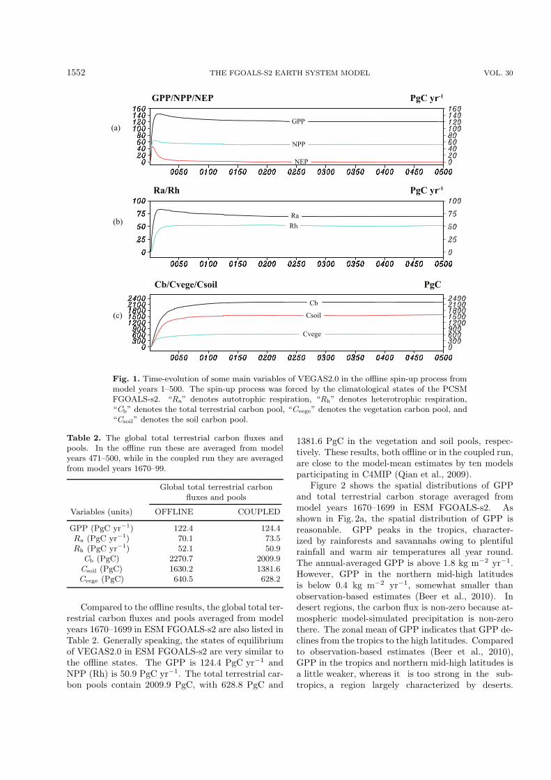
The time series of some main variables in VE-GAS2.0 in the offline step from model years 1–500 arepresented in Fig. 1. In this run, we turned on the ac-celerator (which can increase the time step for slowprocesses to quickly reach the equilibrium) for the soilcarbon pools to make them reach equilibrium as fastas possible for the first 200 years. All the variablesvaried little for the last 300 years. In Figs. 1a andb, the global total terrestrial gross primary produc-tion (GPP) is 122.4 PgC yr−1 (Table 2), correspondingto the observation-based estimate of 123±8 PgC yr−1

provided by Beer et al. (2010). Autotrophic respira-tion (Ra) is 70.1 PgC yr−1. According to the equation

NPP = GPP − Ra , (1)

where NPP denotes net primary production, thesimulated global total terrestrial NPP has a valueof 52.3 PgC yr−1, which lies within the rangeof 44.4–66.3 PgC yr−1 (Cramer et al., 1999).Considering heterotrophic respiration (Rh) is equiv-alent to 52.1 PgC yr−1, the net ecosystem production(NEP) is near to zero, showing the model has reachedequilibrium. Figure 1c indicates the processes of car-bon accumulation in the vegetation and soil pools dur-ing the offline spinup. In summary, the total terres-trial carbon pools simulated in VEGAS2.0 store 2270.7PgC, comprising 640.5 PgC in the vegetation poolsand 1630.2 PgC in the soil (Table 2).

Table 1. Experimental design for the OFFLINE and COUPLED runs.

Experiment name Forcing fields/boundary conditions Active models

OFFLINE Climatological daily forcing fields of PCSM Land component of PCSM FGOALS-s2FGOALS-s2 in the pre-industrial run and VEGAS2.0

COUPLED Boundary conditions in the pre-industrial run PCSM FGOALS-s2 and VEGAS2.0(greenhouse gases, solar constant, aerosol, ozone)


(a)

(b)

(c)

GPP

NPP

NEP

RaRh

Cb

Cvege

Csoil

GPP/NPP/NEP PgC yr-1

Ra/Rh PgC yr-1

Cb/Cvege/Csoil PgC

Fig. 1. Time-evolution of some main variables of VEGAS2.0 in the offline spin-up process frommodel years 1–500. The spin-up process was forced by the climatological states of the PCSMFGOALS-s2. “Ra” denotes autotrophic respiration, “Rh” denotes heterotrophic respiration,“Cb” denotes the total terrestrial carbon pool, “Cvege” denotes the vegetation carbon pool, and“Csoil” denotes the soil carbon pool.

Table 2. The global total terrestrial carbon fluxes andpools. In the offline run these are averaged from modelyears 471–500, while in the coupled run they are averagedfrom model years 1670–99.

Global total terrestrial carbonfluxes and pools

Variables (units) OFFLINE COUPLED

GPP (PgC yr−1) 122.4 124.4Ra (PgC yr−1) 70.1 73.5Rh (PgC yr−1) 52.1 50.9

Cb (PgC) 2270.7 2009.9Csoil (PgC) 1630.2 1381.6Cvege (PgC) 640.5 628.2

Compared to the offline results, the global total ter-restrial carbon fluxes and pools averaged from modelyears 1670–1699 in ESM FGOALS-s2 are also listed inTable 2. Generally speaking, the states of equilibriumof VEGAS2.0 in ESM FGOALS-s2 are very similar tothe offline states. The GPP is 124.4 PgC yr−1 andNPP (Rh) is 50.9 PgC yr−1. The total terrestrial car-bon pools contain 2009.9 PgC, with 628.8 PgC and

1381.6 PgC in the vegetation and soil pools, respec-tively. These results, both offline or in the coupled run,are close to the model-mean estimates by ten modelsparticipating in C4MIP (Qian et al., 2009).

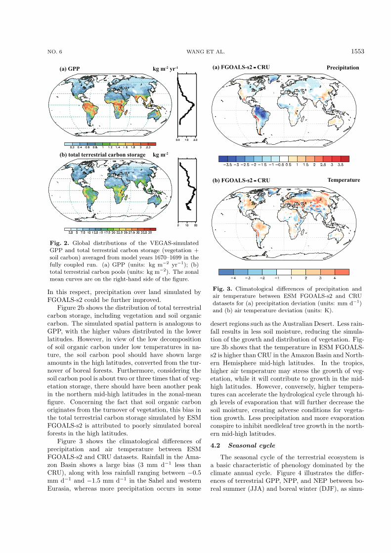
Figure 2 shows the spatial distributions of GPPand total terrestrial carbon storage averaged frommodel years 1670–1699 in ESM FGOALS-s2. Asshown in Fig. 2a, the spatial distribution of GPP isreasonable. GPP peaks in the tropics, character-ized by rainforests and savannahs owing to plentifulrainfall and warm air temperatures all year round.The annual-averaged GPP is above 1.8 kg m−2 yr−1.However, GPP in the northern mid-high latitudesis below 0.4 kg m−2 yr−1, somewhat smaller thanobservation-based estimates (Beer et al., 2010). Indesert regions, the carbon flux is non-zero because at-mospheric model-simulated precipitation is non-zerothere. The zonal mean of GPP indicates that GPP de-clines from the tropics to the high latitudes. Comparedto observation-based estimates (Beer et al., 2010),GPP in the tropics and northern mid-high latitudes isa little weaker, whereas it is too strong in the sub-tropics, a region largely characterized by deserts.


(a) GPP kg m-2 yr-1

(b) total terrestrial carbon storage kg m-2

Fig. 2. Global distributions of the VEGAS-simulatedGPP and total terrestrial carbon storage (vegetation +soil carbon) averaged from model years 1670–1699 in thefully coupled run. (a) GPP (units: kg m−2 yr−1); (b)total terrestrial carbon pools (units: kg m−2). The zonalmean curves are on the right-hand side of the figure.

In this respect, precipitation over land simulated byFGOALS-s2 could be further improved.

Figure 2b shows the distribution of total terrestrialcarbon storage, including vegetation and soil organiccarbon. The simulated spatial pattern is analogous toGPP, with the higher values distributed in the lowerlatitudes. However, in view of the low decompositionof soil organic carbon under low temperatures in na-ture, the soil carbon pool should have shown largeamounts in the high latitudes, converted from the tur-nover of boreal forests. Furthermore, considering thesoil carbon pool is about two or three times that of veg-etation storage, there should have been another peakin the northern mid-high latitudes in the zonal-meanfigure. Concerning the fact that soil organic carbonoriginates from the turnover of vegetation, this bias inthe total terrestrial carbon storage simulated by ESMFGOALS-s2 is attributed to poorly simulated borealforests in the high latitudes.

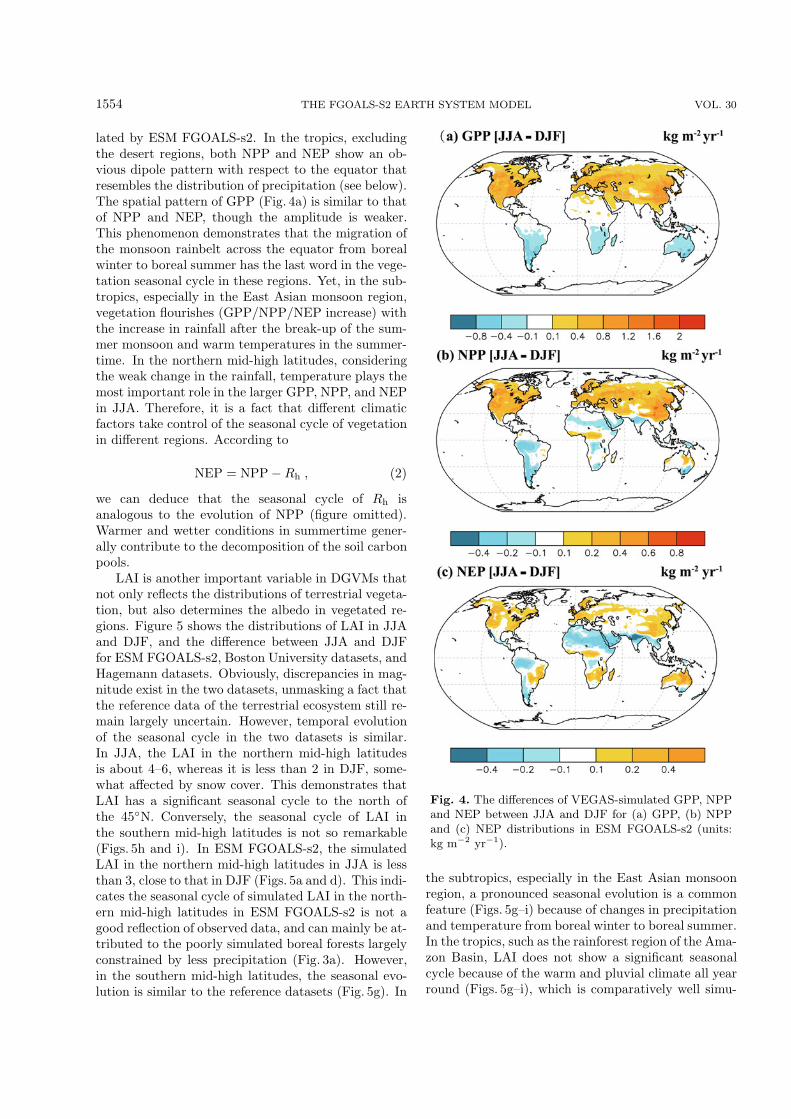
Figure 3 shows the climatological differences ofprecipitation and air temperature between ESMFGOALS-s2 and CRU datasets. Rainfall in the Ama-zon Basin shows a large bias (3 mm d−1 less thanCRU), along with less rainfall ranging between −0.5mm d−1 and −1.5 mm d−1 in the Sahel and westernEurasia, whereas more precipitation occurs in some

(a) FGOALS-s2 -- CRU Precipitation

(b) FGOALS-s2 -- CRU Temperature

Fig. 3. Climatological differences of precipitation andair temperature between ESM FGOALS-s2 and CRUdatasets for (a) precipitation deviation (units: mm d−1)and (b) air temperature deviation (units: K).

desert regions such as the Australian Desert. Less rain-fall results in less soil moisture, reducing the simula-tion of the growth and distribution of vegetation. Fig-ure 3b shows that the temperature in ESM FGOALS-s2 is higher than CRU in the Amazon Basin and North-ern Hemisphere mid-high latitudes. In the tropics,higher air temperature may stress the growth of veg-etation, while it will contribute to growth in the mid-high latitudes. However, conversely, higher tempera-tures can accelerate the hydrological cycle through hi-gh levels of evaporation that will further decrease thesoil moisture, creating adverse conditions for vegeta-tion growth. Less precipitation and more evaporationconspire to inhibit needleleaf tree growth in the north-ern mid-high latitudes.

4.2 Seasonal cycle

The seasonal cycle of the terrestrial ecosystem isa basic characteristic of phenology dominated by theclimate annual cycle. Figure 4 illustrates the differ-ences of terrestrial GPP, NPP, and NEP between bo-real summer (JJA) and boreal winter (DJF), as simu-


lated by ESM FGOALS-s2. In the tropics, excludingthe desert regions, both NPP and NEP show an ob-vious dipole pattern with respect to the equator thatresembles the distribution of precipitation (see below).The spatial pattern of GPP (Fig. 4a) is similar to thatof NPP and NEP, though the amplitude is weaker.This phenomenon demonstrates that the migration ofthe monsoon rainbelt across the equator from borealwinter to boreal summer has the last word in the vege-tation seasonal cycle in these regions. Yet, in the sub-tropics, especially in the East Asian monsoon region,vegetation flourishes (GPP/NPP/NEP increase) withthe increase in rainfall after the break-up of the sum-mer monsoon and warm temperatures in the summer-time. In the northern mid-high latitudes, consideringthe weak change in the rainfall, temperature plays themost important role in the larger GPP, NPP, and NEPin JJA. Therefore, it is a fact that different climaticfactors take control of the seasonal cycle of vegetationin different regions. According to

NEP = NPP − Rh , (2)

we can deduce that the seasonal cycle of Rh isanalogous to the evolution of NPP (figure omitted).Warmer and wetter conditions in summertime gener-ally contribute to the decomposition of the soil carbonpools.

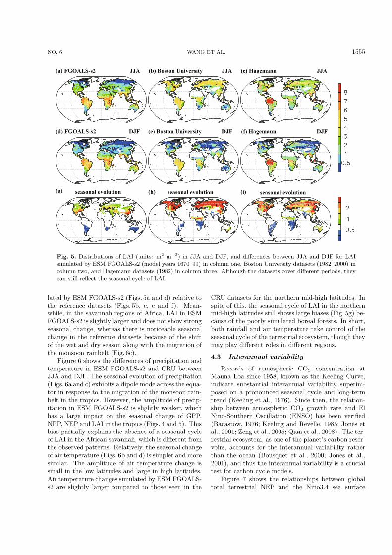
LAI is another important variable in DGVMs thatnot only reflects the distributions of terrestrial vegeta-tion, but also determines the albedo in vegetated re-gions. Figure 5 shows the distributions of LAI in JJAand DJF, and the difference between JJA and DJFfor ESM FGOALS-s2, Boston University datasets, andHagemann datasets. Obviously, discrepancies in mag-nitude exist in the two datasets, unmasking a fact thatthe reference data of the terrestrial ecosystem still re-main largely uncertain. However, temporal evolutionof the seasonal cycle in the two datasets is similar.In JJA, the LAI in the northern mid-high latitudesis about 4–6, whereas it is less than 2 in DJF, some-what affected by snow cover. This demonstrates thatLAI has a significant seasonal cycle to the north ofthe 45◦N. Conversely, the seasonal cycle of LAI inthe southern mid-high latitudes is not so remarkable(Figs. 5h and i). In ESM FGOALS-s2, the simulatedLAI in the northern mid-high latitudes in JJA is lessthan 3, close to that in DJF (Figs. 5a and d). This indi-cates the seasonal cycle of simulated LAI in the north-ern mid-high latitudes in ESM FGOALS-s2 is not agood reflection of observed data, and can mainly be at-tributed to the poorly simulated boreal forests largelyconstrained by less precipitation (Fig. 3a). However,in the southern mid-high latitudes, the seasonal evo-lution is similar to the reference datasets (Fig. 5g). In

Fig. 4. The differences of VEGAS-simulated GPP, NPPand NEP between JJA and DJF for (a) GPP, (b) NPPand (c) NEP distributions in ESM FGOALS-s2 (units:kg m−2 yr−1).

the subtropics, especially in the East Asian monsoonregion, a pronounced seasonal evolution is a commonfeature (Figs. 5g–i) because of changes in precipitationand temperature from boreal winter to boreal summer.In the tropics, such as the rainforest region of the Ama-zon Basin, LAI does not show a significant seasonalcycle because of the warm and pluvial climate all yearround (Figs. 5g–i), which is comparatively well simu-


(a) FGOALS-s2 (b) Boston UniversityJJA JJA (c) Hagemann JJA

(d) FGOALS-s2 DJF (e) Boston University DJF (f) Hagemann DJF

(g) seasonal evolution (h) seasonal evolution (i) seasonal evolution

Fig. 5. Distributions of LAI (units: m2 m−2) in JJA and DJF, and differences between JJA and DJF for LAIsimulated by ESM FGOALS-s2 (model years 1670–99) in column one, Boston University datasets (1982–2000) incolumn two, and Hagemann datasets (1982) in column three. Although the datasets cover different periods, theycan still reflect the seasonal cycle of LAI.

lated by ESM FGOALS-s2 (Figs. 5a and d) relative tothe reference datasets (Figs. 5b, c, e and f). Mean-while, in the savannah regions of Africa, LAI in ESMFGOALS-s2 is slightly larger and does not show strongseasonal change, whereas there is noticeable seasonalchange in the reference datasets because of the shiftof the wet and dry season along with the migration ofthe monsoon rainbelt (Fig. 6c).

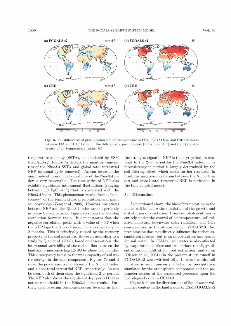
Figure 6 shows the differences of precipitation andtemperature in ESM FGOALS-s2 and CRU betweenJJA and DJF. The seasonal evolution of precipitation(Figs. 6a and c) exhibits a dipole mode across the equa-tor in response to the migration of the monsoon rain-belt in the tropics. However, the amplitude of precip-itation in ESM FGOALS-s2 is slightly weaker, whichhas a large impact on the seasonal change of GPP,NPP, NEP and LAI in the tropics (Figs. 4 and 5). Thisbias partially explains the absence of a seasonal cycleof LAI in the African savannah, which is different fromthe observed patterns. Relatively, the seasonal changeof air temperature (Figs. 6b and d) is simpler and moresimilar. The amplitude of air temperature change issmall in the low latitudes and large in high latitudes.Air temperature changes simulated by ESM FGOALS-s2 are slightly larger compared to those seen in the

CRU datasets for the northern mid-high latitudes. Inspite of this, the seasonal cycle of LAI in the northernmid-high latitudes still shows large biases (Fig. 5g) be-cause of the poorly simulated boreal forests. In short,both rainfall and air temperature take control of theseasonal cycle of the terrestrial ecosystem, though theymay play different roles in different regions.

4.3 Interannual variability

Records of atmospheric CO2 concentration atMauna Loa since 1958, known as the Keeling Curve,indicate substantial interannual variability superim-posed on a pronounced seasonal cycle and long-termtrend (Keeling et al., 1976). Since then, the relation-ship between atmospheric CO2 growth rate and ElNino-Southern Oscillation (ENSO) has been verified(Bacastow, 1976; Keeling and Revelle, 1985; Jones etal., 2001; Zeng et al., 2005; Qian et al., 2008). The ter-restrial ecosystem, as one of the planet’s carbon reser-voirs, accounts for the interannual variability ratherthan the ocean (Bousquet et al., 2000; Jones et al.,2001), and thus the interannual variability is a crucialtest for carbon cycle models.

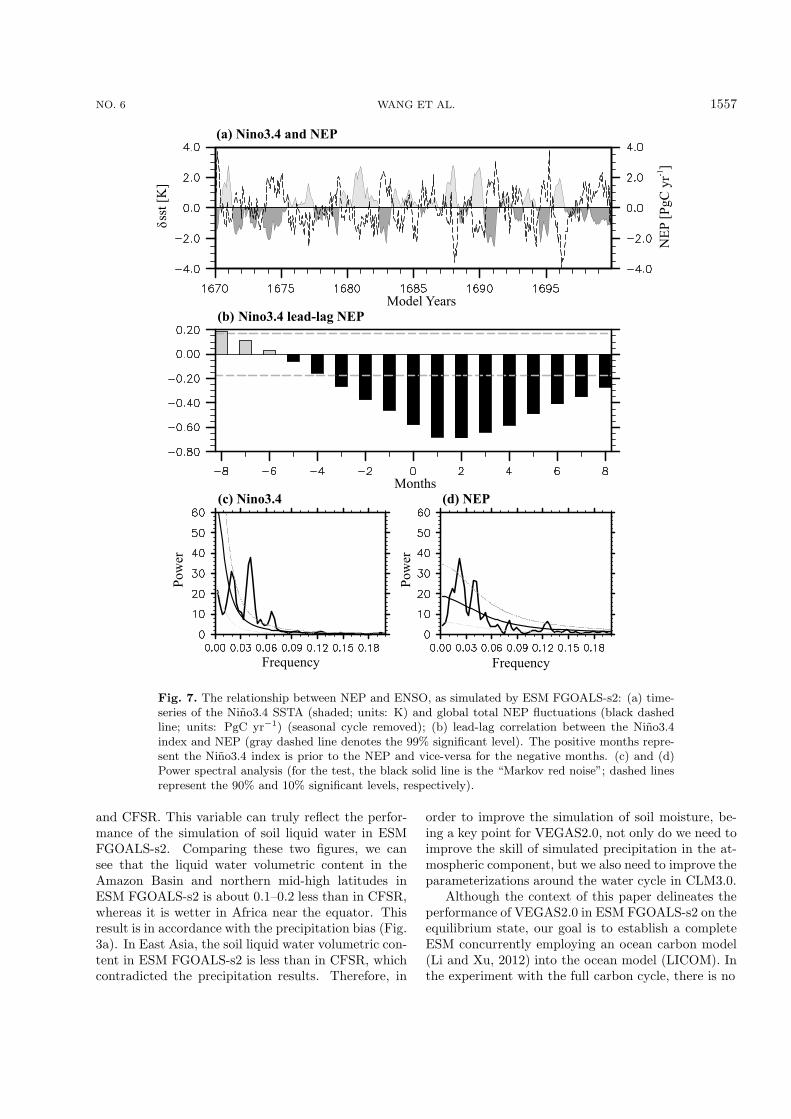
Figure 7 shows the relationships between globaltotal terrestrial NEP and the Nino3.4 sea surface


(a) FGOALS-s2 mm d-1 (b) FGOALS-s2 K

(c) CRU mm d-1 (d) CRU K

Fig. 6. The differences of precipitation and air temperature in ESM FGOALS-s2 and CRU datasetsbetween JJA and DJF for (a, c) the difference of precipitation (units: mm d−1) and (b, d) the dif-ference of air temperature (units: K).

temperature anomaly (SSTA), as simulated by ESMFGOALS-s2. Figure 7a depicts the monthly time se-ries of the Nino3.4 SSTA and global total terrestrialNEP (seasonal cycle removed). As can be seen, theamplitude of interannual variability of the Nino3.4 in-dex is very reasonable. The time series of NEP alsoexhibits significant interannual fluctuations (rangingbetween ±3 PgC yr−1) that is correlated with theNino3.4 index. This phenomenon results from a “con-spiracy” of the temperature, precipitation, and plantsoil physiology (Zeng et al., 2005). However, variationsbetween NEP and the Nino3.4 index are not perfectlyin phase by comparison. Figure 7b shows the lead-lagcorrelation between them. It demonstrates that thenegative correlation peaks with a value of −0.7 whenthe NEP lags the Nino3.4 index for approximately 1–2 months. This is principally caused by the memoryproperty of the soil moisture. However, according to astudy by Qian et al. (2008), based on observations, theinterannual variability of the carbon flux between theland and atmosphere lags ENSO by about 5–6 months.This discrepancy is due to the weak capacity of soil wa-ter storage in the land component. Figures 7c and dshow the power spectral analyses of the Nino3.4 indexand global total terrestrial NEP, respectively. As canbe seen, both of them show the significant 2-yr period.The NEP also shows the significant 4-yr period that isnot so remarkable in the Nino3.4 index results. Fur-ther, an interesting phenomenon can be seen in that

the strongest signal in NEP is the 4-yr period, in con-trast to the 2-yr period for the Nino3.4 index. Thisinconsistency in period is largely determined by thesoil filtering effect, which needs further research. Inbrief, the negative correlation between the Nino3.4 in-dex and global total terrestrial NEP is noticeable inthe fully coupled model.

5. Discussion

As mentioned above, the bias of precipitation in themodel will influence the simulation of the growth anddistribution of vegetation. However, photosynthesis isentirely under the control of air temperature, soil rel-ative moisture, downward solar radiation, and CO2

concentration in the atmosphere in VEGAS2.0. So,precipitation does not directly influence the carbon as-similation process, but is an important surface sourcefor soil water. In CLM3.0, soil water is also affectedby evaporation, surface and sub-surface runoff, gradi-ent diffusion, infiltration, root extraction, and so on(Oleson et al., 2004) (in the present study, runoff inFGOALS-s2 was switched off). In other words, soilmoisture is simultaneously affected by precipitationsimulated by the atmospheric component and the pa-rameterizations of the associated processes upon thehydrological cycle in CLM3.0.

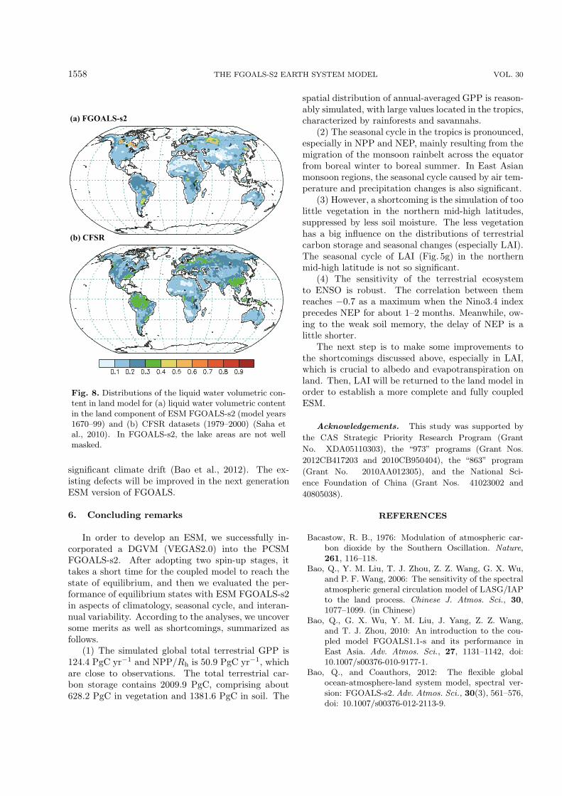
Figure 8 shows the distributions of liquid water vol-umetric content in the land model of ESM FGOALS-s2


Fig. 7. The relationship between NEP and ENSO, as simulated by ESM FGOALS-s2: (a) time-series of the Nino3.4 SSTA (shaded; units: K) and global total NEP fluctuations (black dashedline; units: PgC yr−1) (seasonal cycle removed); (b) lead-lag correlation between the Nino3.4index and NEP (gray dashed line denotes the 99% significant level). The positive months repre-sent the Nino3.4 index is prior to the NEP and vice-versa for the negative months. (c) and (d)Power spectral analysis (for the test, the black solid line is the “Markov red noise”; dashed linesrepresent the 90% and 10% significant levels, respectively).

and CFSR. This variable can truly reflect the perfor-mance of the simulation of soil liquid water in ESMFGOALS-s2. Comparing these two figures, we cansee that the liquid water volumetric content in theAmazon Basin and northern mid-high latitudes inESM FGOALS-s2 is about 0.1–0.2 less than in CFSR,whereas it is wetter in Africa near the equator. Thisresult is in accordance with the precipitation bias (Fig.3a). In East Asia, the soil liquid water volumetric con-tent in ESM FGOALS-s2 is less than in CFSR, whichcontradicted the precipitation results. Therefore, in

order to improve the simulation of soil moisture, be-ing a key point for VEGAS2.0, not only do we need toimprove the skill of simulated precipitation in the at-mospheric component, but we also need to improve theparameterizations around the water cycle in CLM3.0.

Although the context of this paper delineates theperformance of VEGAS2.0 in ESM FGOALS-s2 on theequilibrium state, our goal is to establish a completeESM concurrently employing an ocean carbon model(Li and Xu, 2012) into the ocean model (LICOM). Inthe experiment with the full carbon cycle, there is no


(a) FGOALS-s2

(b) CFSR

Fig. 8. Distributions of the liquid water volumetric con-tent in land model for (a) liquid water volumetric contentin the land component of ESM FGOALS-s2 (model years1670–99) and (b) CFSR datasets (1979–2000) (Saha etal., 2010). In FGOALS-s2, the lake areas are not wellmasked.

significant climate drift (Bao et al., 2012). The ex-isting defects will be improved in the next generationESM version of FGOALS.

6. Concluding remarks

In order to develop an ESM, we successfully in-corporated a DGVM (VEGAS2.0) into the PCSMFGOALS-s2. After adopting two spin-up stages, ittakes a short time for the coupled model to reach thestate of equilibrium, and then we evaluated the per-formance of equilibrium states with ESM FGOALS-s2in aspects of climatology, seasonal cycle, and interan-nual variability. According to the analyses, we uncoversome merits as well as shortcomings, summarized asfollows.

(1) The simulated global total terrestrial GPP is124.4 PgC yr−1 and NPP/Rh is 50.9 PgC yr−1, whichare close to observations. The total terrestrial car-bon storage contains 2009.9 PgC, comprising about628.2 PgC in vegetation and 1381.6 PgC in soil. The

spatial distribution of annual-averaged GPP is reason-ably simulated, with large values located in the tropics,characterized by rainforests and savannahs.

(2) The seasonal cycle in the tropics is pronounced,especially in NPP and NEP, mainly resulting from themigration of the monsoon rainbelt across the equatorfrom boreal winter to boreal summer. In East Asianmonsoon regions, the seasonal cycle caused by air tem-perature and precipitation changes is also significant.

(3) However, a shortcoming is the simulation of toolittle vegetation in the northern mid-high latitudes,suppressed by less soil moisture. The less vegetationhas a big influence on the distributions of terrestrialcarbon storage and seasonal changes (especially LAI).The seasonal cycle of LAI (Fig. 5g) in the northernmid-high latitude is not so significant.

(4) The sensitivity of the terrestrial ecosystemto ENSO is robust. The correlation between themreaches −0.7 as a maximum when the Nino3.4 indexprecedes NEP for about 1–2 months. Meanwhile, ow-ing to the weak soil memory, the delay of NEP is alittle shorter.

The next step is to make some improvements tothe shortcomings discussed above, especially in LAI,which is crucial to albedo and evapotranspiration onland. Then, LAI will be returned to the land model inorder to establish a more complete and fully coupledESM.

Acknowledgements. This study was supported by

the CAS Strategic Priority Research Program (Grant

No. XDA05110303), the “973” programs (Grant Nos.

2012CB417203 and 2010CB950404), the “863” program

(Grant No. 2010AA012305), and the National Sci-

ence Foundation of China (Grant Nos. 41023002 and

40805038).

REFERENCES

Bacastow, R. B., 1976: Modulation of atmospheric car-bon dioxide by the Southern Oscillation. Nature,261, 116–118.

Bao, Q., Y. M. Liu, T. J. Zhou, Z. Z. Wang, G. X. Wu,and P. F. Wang, 2006: The sensitivity of the spectralatmospheric general circulation model of LASG/IAPto the land process. Chinese J. Atmos. Sci., 30,1077–1099. (in Chinese)

Bao, Q., G. X. Wu, Y. M. Liu, J. Yang, Z. Z. Wang,and T. J. Zhou, 2010: An introduction to the cou-pled model FGOALS1.1-s and its performance inEast Asia. Adv. Atmos. Sci., 27, 1131–1142, doi:10.1007/s00376-010-9177-1.

Bao, Q., and Coauthors, 2012: The flexible globalocean-atmosphere-land system model, spectral ver-sion: FGOALS-s2. Adv. Atmos. Sci., 30(3), 561–576,doi: 10.1007/s00376-012-2113-9.


Beer, C., and Coauthors, 2010: Terrestrial gross carbondioxide uptake: Global distribution and covariationwith climate. Science, 329, 834–838.

Bousquet, P., P. Peylin, P. Ciais, C. L. Quere, P.Friedlingstein, and P. P. Tans, 2000: Regionalchanges in cabon dioxide fluxes of land and oceanssince 1980. Science, 290, 1342–1346.

Brovkin, V., A. Ganopolski, and Y. Svirezhev, 1997: Acontinuous climate-vegetation classification for use inclimate-biosphere studies. Ecological Modelling, 101,251–261.

Collins, W. D., and Coauthors, 2006: The community cli-mate system model version 3 (CCSM3). J. Climate,19, 2122–2143.

Cox, P. M., 2001: Description of the “TRIFFID” dynamicglobal vegetation model. Hadley Center Tech. Note24, 1–16.

Cox, P. M., R. A. Betts, C. D. Jones, S. A. Spall, and I.J. Totterdell, 2000: Acceleration of global warmingdue to carbon-cycle feedbacks in a coupled climatemodel. Nature, 408, 184–187.

Cramer, W., and Coauthors, 1999: Comparing globalmodels of terrestrial net primary productivity(NPP): Overview and key results. Global Change Bi-ology, 5, 1–15.

Denman, K. L., and Coauthors, 2007: Couplings betweenchanges in the climate system and biogeochemistry.Climate Change 2007: The Physical Science Basis.Solomon et al., Eds., Cambridge University Press,Cambridge, 499–587.

Dufresne, J. L., P. Friedlingstein, M. Berthelot, L. Bopp,P. Ciais, L. Fairhead, H. Le Treut, and P. Monfray,2002: On the magnitude of positive feedback betweenfuture climate change and the carbon cycle. Geophys.Res. Lett., 29(10), doi: 10.1029/2001GL013777.

Foley, J. A., I. C. Prentice, N. Ramankutty, S. Levis, D.Pollard, S. Sitch, and A. Haxeltine, 1996: An in-tegrating biosphere model of land surface processes,terrestrial carbon balance, and vegetation dynamics.Global Biogeochemical Cycles, 10, 603–628.

Friedlingstein, P., and Coauthors, 2006: Climate-carboncycle feedback analysis: Results from the C4MIPmodel intercomparison. J. Climate, 19, 3337–3353.

Hagemann, S., 2002: An improved land surface param-eter dataset for global and regional climate models.Max Planck Inst. Meteorol (MPI) Rep., 336, 1–21.

Heimann, M., and M. Reichstein, 2008: Terrestrialecosystem carbon dynamics and climate feedbacks.Nature, 451, 289–292.

Ji, J. J., 1995: A climate-vegetation interaction model:Simulating physical and biological processes at thesurface. Journal of Biogeography, 22, 445–451.

Jones, C. D., M. Collins, P. M. Cox, and S. A. Spall,2001: The carbon cycle response to ENSO: A cou-pled climate-carbon cycle and model study. J. Cli-mate, 14, 4113–4129.

Keeling, C. D., and R. Revelle, 1985: Effects of ELNino/Southern Oscillation on the atmospheric con-tent of carbon dioxide. Meteoritics, 20, 437–450.

Keeling, C. D., R. B. Bacastow, A. E. Bainbridge, C.A. Ekdahl, J. R., P. R. Guenther, and L. S. Water-man, 1976: Atmospheric carbon dioxide variations atMauna Loa pbservatory, Hawaii. Tellus, 28, 538–551.

Levis, S., G. B. Bonan, M. Vertenstein, and K. W. Ole-son, 2004: The community land model’s dynamicglobal vegetation model (CLM-DGVM): Technicaldescription and user’s guide. NCAR Tech. Note,NCAR/TN-459+IA, 64pp.

Li, Y. C., and Y. F. Xu, 2012: Uptake and storage ofanthropogenic CO2 in the Pacific Ocean estimatedusing two modeling approaches. Adv. Atmos. Sci.,29, 795–809, doi: 10.1007/s00376-012-1170-4.

Mitchell, T. D., and P. D. Jones, 2005: An improvedmethod of constructing a database of monthly cli-mate observations and associated high-resolutiongrids. Inter. J. Climatol., 25, 693–712.

Myneni, R. B., R. R. Nemani, and S. W. Running, 1997.Algorithm for the estimation of global land cover,LAI and FPAR based on radiative transfer models.IEEE Trans. Geosc. Remote Sens., 35, 1380–1393.

Oleson, K. W., and Coauthors, 2004: Technical De-scription of the Community Land Model (CLM).NCAR/TN-461+STR, 174pp.

Qian, H. F., R. Joseph, and N. Zeng, 2008: Response ofthe terrestrial carbon cycle to the El Nino-SouthernOscillation. Tellus, 60B, 537–550.

Qian, H. F., R. Joseph, and N. Zeng, 2009: Enhancedterrestrial carbon uptake in the northern high lati-tudes in the 21st century from the coupled carboncycle climate model intercomparison project modelprojections. Global Change Biology, 16, 641–656.

Saha, S., and Coauthors, 2010: The NCEP climate fore-cast system reanalysis. Bull. Amer. Meteor. Soc., 91,1015–1057.

Taylor, K. E., R. J. Stouffer, and G. A. Meehl, 2009: Asummary of the CMIP5 experiment design. [Avail-able online at http://cmip-pcmdi.llnl.gov/cmip5/docs/Taylor CMIP5 design.pdf.]

Zeng, N., 2003: Glacial-interglacial atmospheric CO2

change — The glacial burial hypothesis. Adv. Atmos.Sci., 20, 677–693.

Zeng, N., H. F. Qian, E. Munoz, and R. Iacono, 2004:How strong is carbon cycle-climate feedback underglobal warming? Geophys. Res. Lett., 31, L20203,doi: 10.1029/2004GL020904.

Zeng, N., A. Mariotti, and P. Wetzel, 2005: Ter-restrial mechanisms of interannual CO2 variabil-ity. Global Biogeochemical Cycles, 19, GB1016, doi:10.1029/2004GB002273.

Zhang, X. H., G. Y. Shi, H. Liu, and Y. Q. Yu, 2000:IAP Global Ocean-Atmosphere-Land System Model.Science Press, Beijing, 252pp. (in Chinese)

Documents

Earth System Model FGOALS-s2: Coupling a Dynamic Global