Embed Size (px)
Citation preview

iii
Project Report EO-1-3
Earth Observing-1 Advanced Land Imager: Radiometric Response Calibration
J. A. Mendenhall, D.E. Lencioni, and J. B. Evans
Lincoln Laboratory Massachusetts Institute of Technology
Lexington, Massachusetts
29 November 2000
Prepared for the National Aeronautics and Space Administration under Air Force Contract F19628-00-C-0002.

iv
ABSTRACT
The Advanced Land Imager (ALI) is one of three instruments to be flown on the first Earth Observing mission (EO-1) under NASA’s New Millennium Program (NMP). ALI contains a number of innovative features, including a wide field of view optical design, compact multispectral focal plane arrays, non-cryogenic HgCdTe detectors for the short wave infrared bands, and silicon carbide optics. This document outlines the techniques adopted during ground calibration of the radiometric response of the Advanced Land Imager. Results from system level measurements of the instrument response, signal-to-noise ratio, saturation radiance, and dynamic range for all detectors of every spectral band are also presented.

v

vi
ACKNOWLEDGMENTS The authors wish to thank the following individuals of MIT Lincoln Laboratory: Mr. Patrick Quinn for his assistance in building and testing the radiometric transfer standard and collecting data in the laboratory and Mr. Eric Ringdahl for his technical assistance in the laboratory.

vii

viii
TABLE OF CONTENTS
Abstract........................................................................................................................................................ iv
Acknowledgments .........................................................................................................................................vi
1. Introduction.............................................................................................................................................1
2. Radiometric Calibration Technique ...........................................................................................................5
NIST Traceability........................................................................................................................................6
Error Budget...............................................................................................................................................7
3. Data Collection ........................................................................................................................................9
4. Analysis ................................................................................................................................................11
5. Results ..................................................................................................................................................13
Response Coefficient .................................................................................................................................13
Signal-to-Noise Ratio ................................................................................................................................18
Saturation Radiance...................................................................................................................................24
Dynamic Range.........................................................................................................................................30
6. Internal Reference Lamps.......................................................................................................................37
7. Discussion .............................................................................................................................................39
References ...................................................................................................................................................41

ix

x
LIST OF ILLUSTRATIONS Figure No. Page
Figure 1. ALI Focal Plane Assembly.......................................................................................................................................................... 1
Figure 2: Photograph of ALI Focal Plane Assembly................................................................................................................................. 2
Figure 3: Photograph of populated Sensor Chip Assembly. .................................................................................................................... 2
Figure 4: Normalized visible and near infrared spectral response functions based on subsystem level measurements................ 3
Figure 5: Normalized short wave infrared spectral response functions based on subsystem level measurements......................... 4
Figure 6: Integrating sphere and spectroradiometer used during radiometric calibration of the Advanced Land Imager. ........... 5
Figure 7: Radiometric transfer standard system built at Lincoln Laboratory........................................................................................ 6
Figure 8: Example of linear fit to Band 3 detector 100 data. ................................................................................................................. 12
Figure 9: Radiometric calibration coefficients for Band 1p................................................................................................................... 13
Figure 10: Radiometric calibration coefficients for Band 1. .................................................................................................................. 14
Figure 11: Radiometric calibration coefficients for Band 2. .................................................................................................................. 14
Figure 12: Radiometric calibration coefficients for Band 3. .................................................................................................................. 15
Figure 13: Radiometric calibration coefficients for Band 4. .................................................................................................................. 15
Figure 14: Radiometric calibration coefficients for Band 4p................................................................................................................. 16
Figure 15: Radiometric calibration coefficients for Band 5p................................................................................................................. 16
Figure 16: Radiometric calibration coefficients for Band 5. .................................................................................................................. 17
Figure 17: Radiometric calibration coefficients for Band 7. .................................................................................................................. 17
Figure 18: Radiometric calibration coefficients for the Panchromatic Band...................................................................................... 18
Figure 19: Example of signal-to-noise ratio data for Band 3 detector 100.......................................................................................... 19
Figure 20: Signal-to-noise ratio for Band 1p. ........................................................................................................................................... 19
Figure 21: Signal-to-noise ratio for Band 1. ............................................................................................................................................. 20
Figure 22: Signal-to-noise ratio for Band 2. ............................................................................................................................................. 20
Figure 23: Signal-to-noise ratio for Band 3. ............................................................................................................................................. 21
Figure 24: Signal-to-noise ratio for Band 4. ............................................................................................................................................. 21
Figure 25: Signal-to-noise ratio for Band 4p. ........................................................................................................................................... 22

xi
Figure 26: Signal-to-noise ratio for Band 5p. ........................................................................................................................................... 22
Figure 27: Signal-to-noise ratio for Band 5. ............................................................................................................................................. 23
Figure 28: Signal-to-noise ratio for Band 7. ............................................................................................................................................. 23
Figure 29: Signal-to-noise ratio for the Panchromatic Band.................................................................................................................. 24
Figure 30: Saturation radiance for Band 1p. ............................................................................................................................................. 25
Figure 31: Saturation radiance for Band 1. ............................................................................................................................................... 25
Figure 32: Saturation radiance for Band 2. ............................................................................................................................................... 26
Figure 33: Saturation radiance for Band 3. ............................................................................................................................................... 26
Figure 34: Saturation radiance for Band 4. ............................................................................................................................................... 27
Figure 35: Saturation radiance for Band 4p. ............................................................................................................................................. 27
Figure 36: Saturation radiance for Band 5p. ............................................................................................................................................. 28
Figure 37: Saturation radiance for Band 5. ............................................................................................................................................... 28
Figure 38: Saturation radiance for Band 7. ............................................................................................................................................... 29
Figure 39: Saturation radiance for the Panchromatic Band.................................................................................................................... 29
Figure 40: Dynamic range for Band 1p. .................................................................................................................................................... 30
Figure 41: Dynamic range for Band 1........................................................................................................................................................ 31
Figure 42: Dynamic range for Band 2........................................................................................................................................................ 31
Figure 43: Dynamic range for Band 3........................................................................................................................................................ 32
Figure 44: Dynamic range for Band 4........................................................................................................................................................ 32
Figure 45: Dynamic range for Band 4p. .................................................................................................................................................... 33
Figure 46: Dynamic range for Band 5p. .................................................................................................................................................... 33
Figure 47: Dynamic range for Band 5........................................................................................................................................................ 34
Figure 48: Dynamic range for Band 7........................................................................................................................................................ 34
Figure 49: Dynamic range for the Panchromatic Band........................................................................................................................... 35
Figure 50: EO -1 ALI internal reference source........................................................................................................................................ 37
Figure 51: Photograph of internal reference source................................................................................................................................. 37
Figure 52: Band 4 image of Lincoln Laboratory ...................................................................................................................................... 39

xii
LIST OF TABLES
Table No. Page
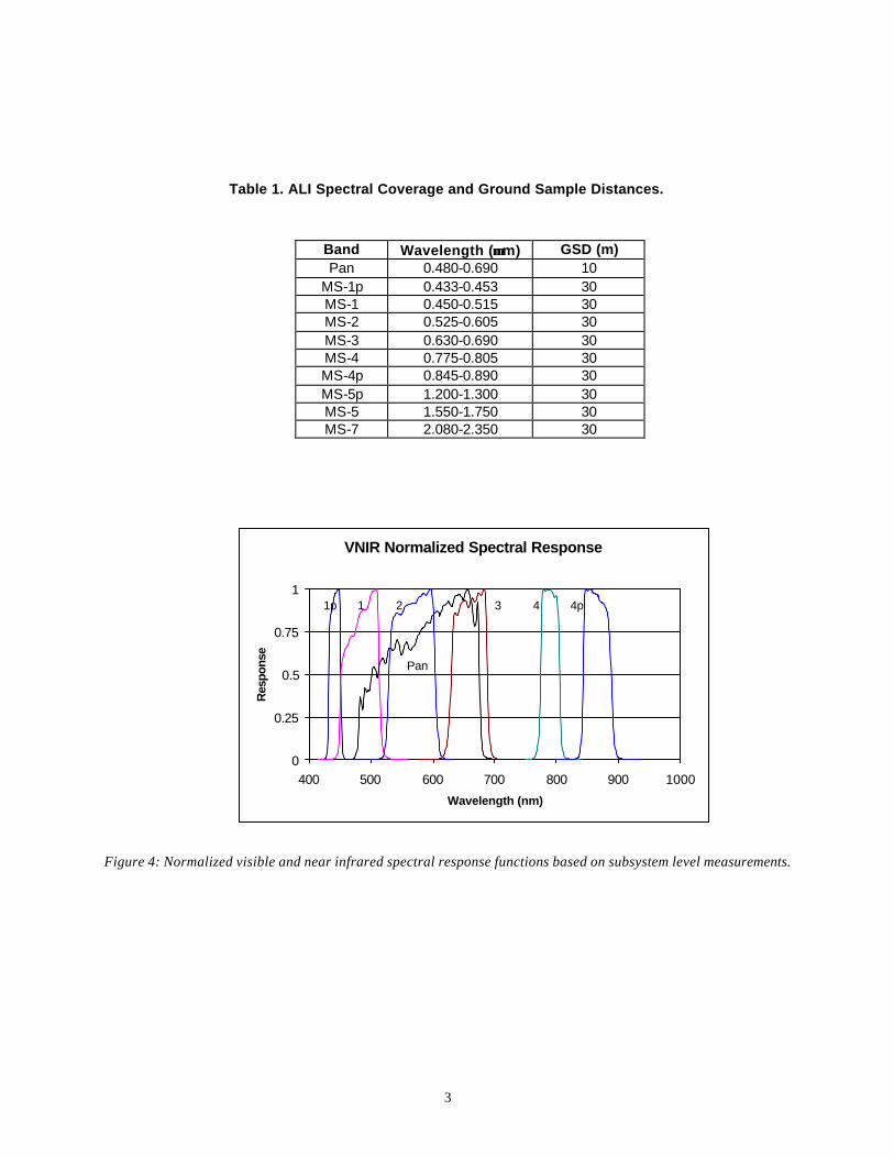
Table 1. ALI Spectral Coverage and Ground Sample Distances............................................................................................................. 3
Table 2. Radiometric Calibration Error Budget. ........................................................................................................................................ 7

xiii
1
1. INTRODUCTION
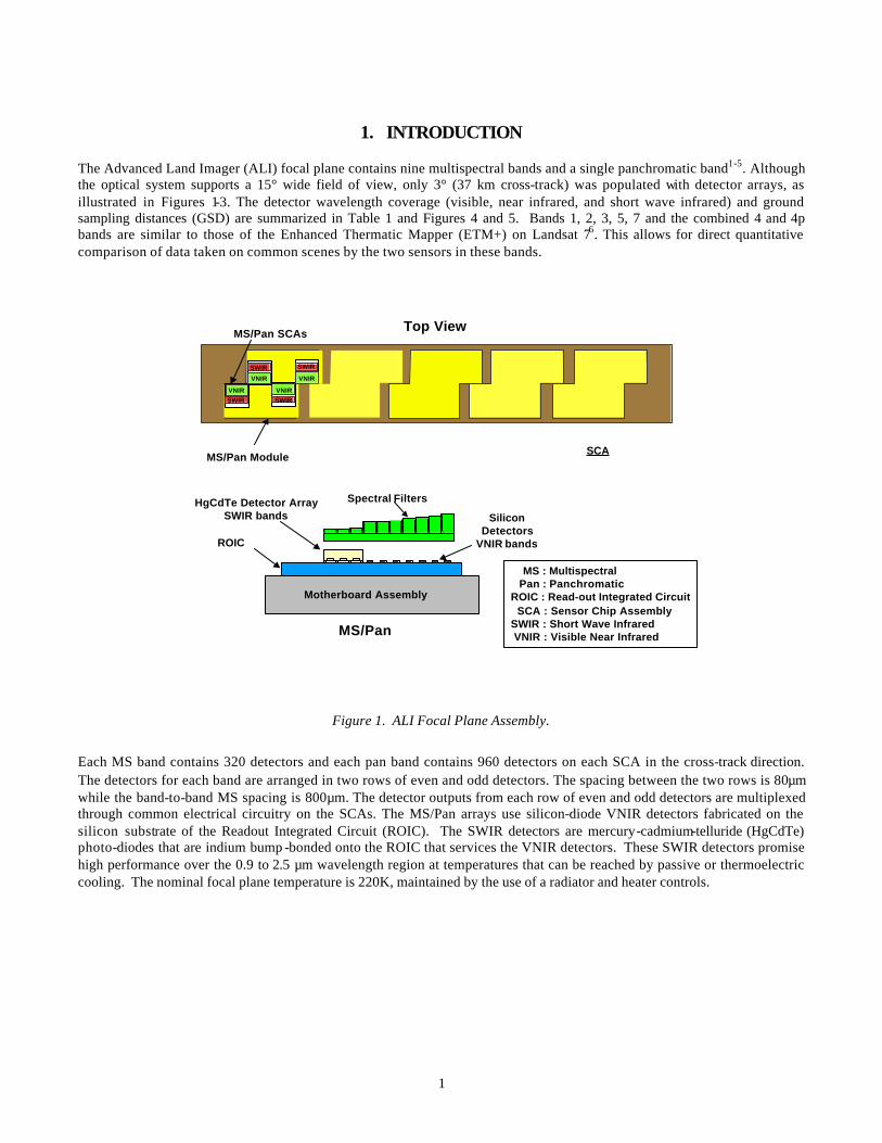
The Advanced Land Imager (ALI) focal plane contains nine multispectral bands and a single panchromatic band1-5. Although the optical system supports a 15° wide field of view, only 3° (37 km cross-track) was populated with detector arrays, as illustrated in Figures 1-3. The detector wavelength coverage (visible, near infrared, and short wave infrared) and ground sampling distances (GSD) are summarized in Table 1 and Figures 4 and 5. Bands 1, 2, 3, 5, 7 and the combined 4 and 4p bands are similar to those of the Enhanced Thermatic Mapper (ETM+) on Landsat 76. This allows for direct quantitative comparison of data taken on common scenes by the two sensors in these bands.
Top View
VNIRSWIR
MS/Pan SCAs
VNIR VNIR
VNIRSWIR
SWIRSWIR
MS/Pan Module
SiliconDetectors
VNIR bands
HgCdTe Detector ArraySWIR bands
Motherboard Assembly
Spectral Filters
MS/Pan
ROIC
MS : Multispectral Pan : PanchromaticROIC : Read-out Integrated Circuit SCA : Sensor Chip AssemblySWIR : Short Wave Infrared VNIR : Visible Near Infrared
•••SCA
Figure 1. ALI Focal Plane Assembly.
Each MS band contains 320 detectors and each pan band contains 960 detectors on each SCA in the cross-track direction. The detectors for each band are arranged in two rows of even and odd detectors. The spacing between the two rows is 80µm while the band-to-band MS spacing is 800µm. The detector outputs from each row of even and odd detectors are multiplexed through common electrical circuitry on the SCAs. The MS/Pan arrays use silicon-diode VNIR detectors fabricated on the silicon substrate of the Readout Integrated Circuit (ROIC). The SWIR detectors are mercury-cadmium-telluride (HgCdTe) photo-diodes that are indium bump -bonded onto the ROIC that services the VNIR detectors. These SWIR detectors promise high performance over the 0.9 to 2.5 µm wavelength region at temperatures that can be reached by passive or thermoelectric cooling. The nominal focal plane temperature is 220K, maintained by the use of a radiator and heater controls.
2
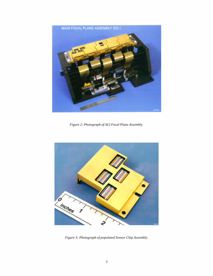
Figure 2: Photograph of ALI Focal Plane Assembly.
Figure 3: Photograph of populated Sensor Chip Assembly.
3
Table 1. ALI Spectral Coverage and Ground Sample Distances.
Band Wavelength (µµm) GSD (m) Pan 0.480-0.690 10
MS-1p 0.433-0.453 30 MS-1 0.450-0.515 30 MS-2 0.525-0.605 30 MS-3 0.630-0.690 30 MS-4 0.775-0.805 30 MS-4p 0.845-0.890 30 MS-5p 1.200-1.300 30 MS-5 1.550-1.750 30 MS-7 2.080-2.350 30
VNIR Normalized Spectral Response
0
0.25
0.5
0.75
1
400 500 600 700 800 900 1000
Wavelength (nm)
Res
pons
e
1p 1 2 3 4 4p
Pan
Figure 4: Normalized visible and near infrared spectral response functions based on subsystem level measurements.

4
SWIR Normalized Spectral Response
0
0.25
0.5
0.75
1
1000 1250 1500 1750 2000 2250 2500
Wavelength (nm)
Res
pons
e
5p 5 7
Figure 5: Normalized short wave infrared spectral response functions based on subsystem level measurements.
Ground calibration of the Advanced Land Imager occurred from September 1998 through January 1999 at the Massachusetts Institute of Technology Lincoln Laboratory7-10. Included in this characterization period was the radiometric calibration of individual detectors at the system level. This report provides a review of the technique employed during radiometric calibration and the results from the characterization of the radiometric response, signal-to-noise ratio, saturation radiance, and dynamic range of each detector.
5
2. RADIOMETRIC CALIBRATION TECHNIQUE
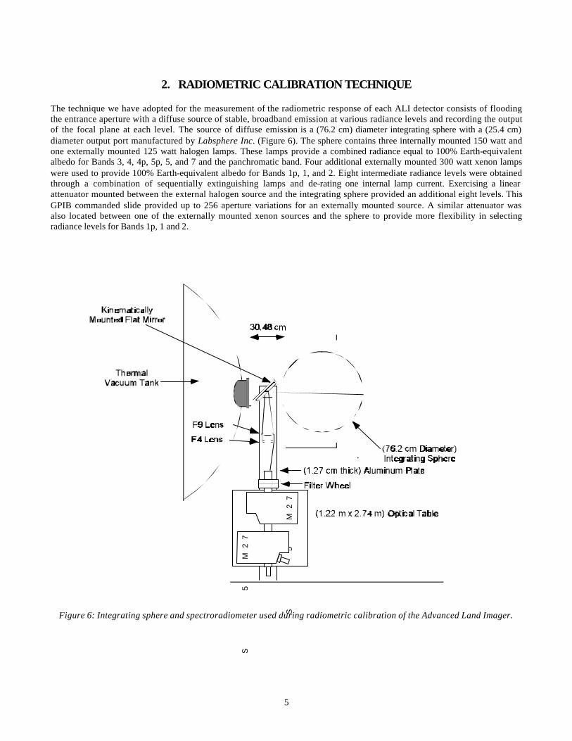
The technique we have adopted for the measurement of the radiometric response of each ALI detector consists of flooding the entrance aperture with a diffuse source of stable, broadband emission at various radiance levels and recording the output of the focal plane at each level. The source of diffuse emission is a (76.2 cm) diameter integrating sphere with a (25.4 cm) diameter output port manufactured by Labsphere Inc. (Figure 6). The sphere contains three internally mounted 150 watt and one externally mounted 125 watt halogen lamps. These lamps provide a combined radiance equal to 100% Earth-equivalent albedo for Bands 3, 4, 4p, 5p, 5, and 7 and the panchromatic band. Four additional externally mounted 300 watt xenon lamps were used to provide 100% Earth-equivalent albedo for Bands 1p, 1, and 2. Eight intermediate radiance levels were obtained through a combination of sequentially extinguishing lamps and de-rating one internal lamp current. Exercising a linear attenuator mounted between the external halogen source and the integrating sphere provided an additional eight levels. This GPIB commanded slide provided up to 256 aperture variations for an externally mounted source. A similar attenuator was also located between one of the externally mounted xenon sources and the sphere to provide more flexibility in selecting radiance levels for Bands 1p, 1 and 2.
Figure 6: Integrating sphere and spectroradiometer used during radiometric calibration of the Advanced Land Imager.
MS
25
7
MS
25
7

6
NIST Traceability In order to provide absolute radiometric traceability to other sensors, a radiometric transfer standard system was constructed at Lincoln Laboratory (Figures 6 and 7). The principal components of the system are an irradiance source, traceable to the National Institute of Standards and Technology (NIST), and an Oriel MS257 monochromator used as a spectroradiometer. The 250 watt irradiance source was mounted on a post with proper baffling to control stray light from the room and reflections from the source off other surfaces. A standard radiance scene was generated by placing a Labsphere Spectralon sheet 50 cm from the irradiance source. The monochromator field-of-view was limited to a 6.45 cm2 region of the diffuse scene to maintain the traceability of the radiance source. A (15.24 cm) flat mirror was placed between the Spectralon diffuser and entrance slit of the monochromator for convenient location of the source. Alternately scanning the radiance scene produced by the standard lamp and various radiance levels output by the large integrating sphere, radiometric NIST traceability was established for the Advanced Land Imager. Additional near real-time monitoring of the sphere radiance level was accomplished by mounting the (15.24 cm) flat mirror on a (30.48 cm) post between the vacuum tank window and the integrating sphere. During radiometric calibration of the ALI, the mirror was removed and the response of the focal plane recorded. Between ALI data collections, the mirror was kinematically mounted on the aluminum bar, redirecting a portion of the sphere radiance into the entrance slit of the spectroradiometer. The radiance of the integrating sphere was measured from 300 to 2500 nm in 10 nm intervals with 5 nm full-width-half-maximum resolution. Finally, silicon and germanium detectors, mechanically mounted to the sphere wall, provided continuous broadband monitoring of the sphere stability.
Figure 7: Radiometric transfer standard system built at Lincoln Laboratory.
MS
257
MS
257
Kin em aticallyMounted Flat Mirror
F9 L ens
F4 Le ns
25 0 W N IST T ra ceabl eIrrad iance So urc e
Baff le
Ba ff le
Spec tralo n She et
Si licon D etec tor
Pb S D etec to r
F ilter W hee l
(1.27 cm thick) Aluminum Plate
(1.22 m x 2.74 m)Optical Tab le
7
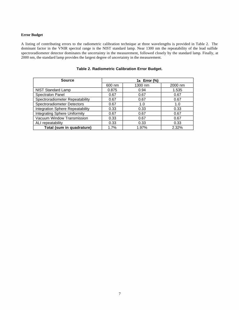
Error Budget A listing of contributing errors to the radiometric calibration technique at three wavelengths is provided in Table 2. The dominant factor in the VNIR spectral range is the NIST standard lamp. Near 1300 nm the repeatability of the lead sulfide spectroradiometer detector dominates the uncertainty in the measurement, followed closely by the standard lamp. Finally, at 2000 nm, the standard lamp provides the largest degree of uncertainty in the measurement.
Table 2. Radiometric Calibration Error Budget.
1σσ Error (%) Source
600 nm 1300 nm 2000 nm NIST Standard Lamp 0.875 0.94 1.535 Spectralon Panel 0.67 0.67 0.67 Spectroradiometer Repeatability 0.67 0.67 0.67 Spectroradiometer Detectors 0.67 1.0 1.0 Integration Sphere Repeatability 0.33 0.33 0.33 Integrating Sphere Uniformity 0.67 0.67 0.67 Vacuum Window Transmission 0.33 0.67 0.67 ALI repeatability 0.33 0.33 0.33
Total (sum in quadrature) 1.7% 1.97% 2.32%

8

9
3. DATA COLLECTION
Radiometric data were collected in January 1999 in a class 1,000 clean room at Lincoln Laboratory. This calibration was conducted with the ALI as a fully assembled instrument in a thermal vacuum chamber at operational temperatures. Selection of the integrating sphere radiance level and monitoring of radiance stability was coordinated by the ALI Calibration Control Node (ACCN), a LabVIEW -based personal computer operating on a Windows 95 platform. Commanding and housekeeping monitoring of the ALI was also controlled by the ACCN via a Goddard Space Flight Center-provided RS2000 Advanced Spacecraft Integration and Systems Test (ASIST) computer. Data acquisition was performed by a Unix-based Electrical Ground Support Equipment (EGSE1) computer. A Silicon Graphics Performance Assessment Machine (PAM) stored and processed focal plane data in real time for quick look assessment. For each radiance level selected, the sphere was allowed to stabilize for one hour. A spectroradiometric scan of the sphere output from 300 – 2500 nm was then conducted after placing a (15.24 cm diameter) flat mirror between the sphere exit port and vacuum tank window to redirect the beam into the monochromator. After the mirror was removed, the response of the focal plane was recorded for several integration periods [0.81 (0.27), 1.35 (0.45), 1.89 (0.63), 2.97 (0.99), 3.51 (1.17), and 4.05 (1.35) milliseconds for MS (Pan) detectors]. Finally, the ALI aperture cover was closed and reference dark frames were recorded for identical integration periods. Data were collected with the ALI illuminated by a combination of halogen sources only, a combination xenon sources only, and a combination of halogen and xenon sources. Additional data were collected using the halogen sources only with the focal plane operating at two other possible operating temperatures (215 K and 225 K) to assess the effects of temperature on focal plane response.

10

11
4. ANALYSIS
Analysis of the radiometric response of the Advanced Land Imager has been divided into three categories: VNIR, leaky, and SWIR. The VNIR and SWIR analysis was separated due to the differing detectors used in these bands (silicon for VNIR, HgCdTe for SWIR). The leaky detector category refers to Band 2 of SCA 4 and Band 3 of SCA 3. Odd detectors of Band 2, SCA 4 exhibit substantial optical or electrical cross-talk when detector 1149 is illuminated. Similarly, even detectors of Band 3, SCA 3 exhibit substantial optical or electrical cross-talk when detector 864 is illuminated. An empirical correction methodology has been developed to effectively remove all traces of the cross-talk and transfer detector responses of these bands into units of radiance (see Earth Observing-1 Advanced Land Imager: Leaky Detector Calibration and Correction). As a result, calibration results for odd detectors of SCA 4 Band 2 and even detectors of SCA 3 Band 3 will not be reviewed in this paper. For VNIR and SWIR data, a linear function was fitted to the response of each detector to incident radiance after subtraction of the dark current. This fit may be expressed as
][),( , darkIillumP PPBIBL −=λ .
Here, Lλ(B,I) is the incident band weighted spectral radiance for Band B and sphere level I, Bp is the radiometric calibration coefficient for detector P (mW/cm2/sr/µ/DN), Pillum,I is the illuminated detector digital response for sphere level I, and Pdark is the dark detector digital offset. Lλ(B,I) was calculated knowing the output radiance of the integrating sphere, the spectral response of each band, and the spectral transmission of the vacuum tank window. This may be expressed analytically as
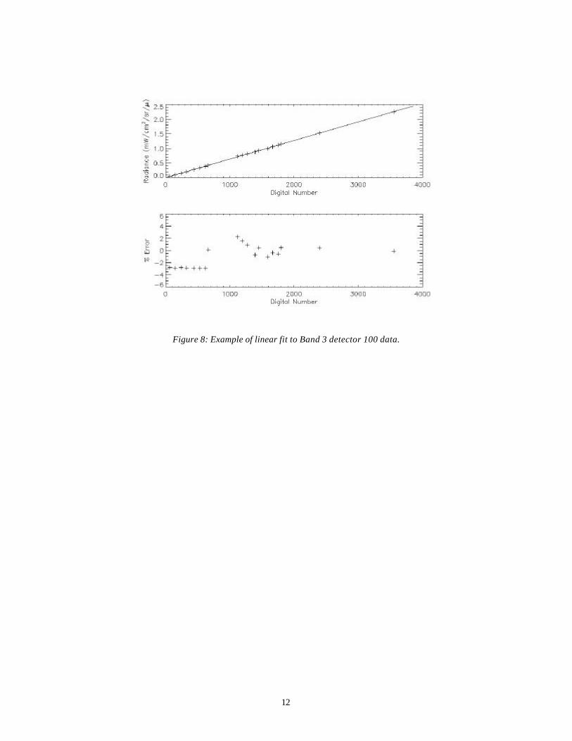
Here, Lλ(λ,I) is the spectroradiometrically measured output radiance of the sphere for level I, TW is the spectral transmission of the vacuum tank window, and S is the normalized spectral response for Band B. The spectral response of each band used in this analysis was determined during the spectral calibration of the ALI (see Earth Observing-1 Advanced Land Imager: Spectral Response Calibration). An example of a linear fit to the data for detector 100 of Band 3 is provided in Figure 8. In this figure, 20 radiance levels were used to fit the detector response. The top graphic is an overlay of the data points and best-fit linear function (the fit was anchored at zero incident radiance by inserting a synthetic data point of zero digital number (dn) for all detectors). The bottom graphic provides the errors to this fit for all radiometric levels. We find all VNIR, SWIR, and panchromatic radiometric response fits to agree with measurements to within ± 3.5% (peak to peak). This is within the error budget specified in Table 2.
∫∫=
λλ
λλλλλ
λdbS
dbSTILIBL
W
),(
),()(),(),(
12
Figure 8: Example of linear fit to Band 3 detector 100 data.

13
5. RESULTS
The radiometric response of each detector of every band was derived individually using the method defined above. From this calibration, the response coefficient, signal-to-noise ratio, saturation radiance, and dynamic range of the ALI focal plane have been determined. We report the results for a nominal integration time of 4.05 ms (1.35 msec for the Pan) and a focal plane temperature of 220 K. Results for other integration times and focal plane temperatures are reported elsewhere (see Earth Observing-1 Advanced Land Imager: Radiometric Response Calibration Addendum) .
Response Coefficient The response coefficient of each band is provided in Figures 9-18. Detectors 0 through 319 belong to SCA 1 (outboard), detectors 320 through 639 to SCA2, detectors 640 through 959 to SCA3, and detectors 960 through 1279 to SCA 4. SCA-to-SCA and detector-to-detector variability are evident in these figures.
Figure 9: Radiometric calibration coefficients for Band 1p.

14
Figure 10: Radiometric calibration coefficients for Band 1.
Detector 989 of Band 1 has also been identified as having excessive dark current13.
Figure 11: Radiometric calibration coefficients for Band 2.

15
Figure 12: Radiometric calibration coefficients for Band 3.
Figure 13: Radiometric calibration coefficients for Band 4.
16
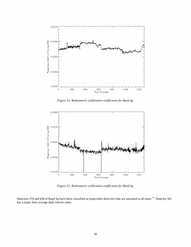
Figure 14: Radiometric calibration coefficients for Band 4p.
Figure 15: Radiometric calibration coefficients for Band 5p.
Detectors 374 and 638 of Band 5p have been classified as inoperable detectors that are saturated at all times 13. Detector 365 has a larger than average dark current value.

17
Figure 16: Radiometric calibration coefficients for Band 5.
Detector 982 is an inoperable detector that exhibits no variation in response with input signal. Detectors 1202, 1204, and 1206 are inoperable detectors that are saturated at all times13. Coefficient variations near detectors 200, 700, and 800 are not associated with any unusual noise or dark current characteristics for this band. Detectors 911 and 913 have larger than average dark current values.
Figure 17: Radiometric calibration coefficients for Band 7.
The large differences present between odd and even detector calibration coefficients for SCA 3 detectors 800-960 are not associated with any unusual noise or dark current characteristics of Band 7.

18
Figure 18: Radiometric calibration coefficients for the Panchromatic Band.
Detector 1631 of the panchromatic band has also been identified as having excessive noise13. Signal-to-Noise Ratio The detector signal-to-noise ratios have been derived from data collected during radiometric calibration. Using the radiometric calibration in-band radiance (mW/cm2/sr/µ) and the detector response and standard deviation data, an individual detector’s signal-to-noise ratio as a function of radiance may be derived. Figure 19 provides an example of the signal-to-noise ratio as a function of radiance for Band 3 detector 100. Below 0.2 mW/cm2/sr/µ, the focal plane noise dominates and results in a linear increase in the signal-to-noise ratio. Above 0.2 mW/cm2/sr/µ, shot noise begins to dominate and the signal-to-noise ratio begins to follow a square root function. The dashed curve in this figure represents a linearly dependent signal-to-noise ratio.

19
Figure 19: Example of signal-to-noise ratio data for Band 3 detector 100.
Fitting the data, a predicted signal-to-noise ratio for any detector may be calculated for any radiance level. Figures 20-29 provide the signal-to-noise ratio for a mid-latitude summer atmosphere, solar zenith angle of 23.50°, 5% surface reflectance, and nadir viewing MODTRAN model. These values are in good agreement with the signal-to-noise ratios calculated from subsystem measurements. Additionally, the increase in signal-to-noise ratio levels for SCA 4 may be attributed to a lower noise for all bands of this SCA.
Figure 20: Signal-to-noise ratio for Band 1p.

20
Figure 21: Signal-to-noise ratio for Band 1.
Detector 989 of Band 1 has a lower response than other detectors, resulting in a lower signal-to-noise ratio compared to its neighbors.
Figure 22: Signal-to-noise ratio for Band 2.

21
Figure 23: Signal-to-noise ratio for Band 3.
Figure 24: Signal-to-noise ratio for Band 4.
22
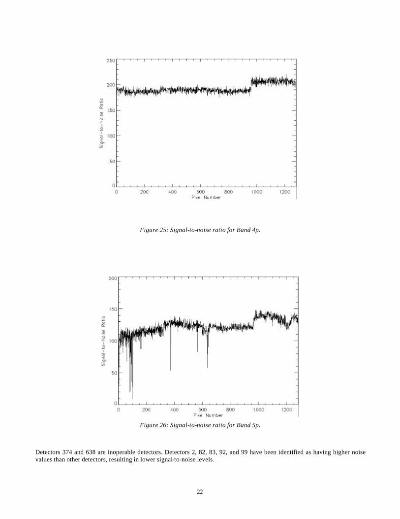
Figure 25: Signal-to-noise ratio for Band 4p.
Figure 26: Signal-to-noise ratio for Band 5p.
Detectors 374 and 638 are inoperable detectors. Detectors 2, 82, 83, 92, and 99 have been identified as having higher noise values than other detectors, resulting in lower signal-to-noise levels.

23
Figure 27: Signal-to-noise ratio for Band 5.
Detectors 982, 1202, 1204, and 1206 are inoperable. The detectors near 200 and 750 DN have lower responses than surrounding detectors. Detector 119 has been identified as having a higher noise value that its neighbors.
Figure 28: Signal-to-noise ratio for Band 7.
24
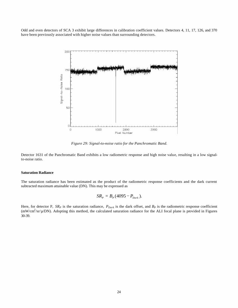
Odd and even detectors of SCA 3 exhibit large differences in calibration coefficient values. Detectors 4, 11, 17, 126, and 370 have been previously associated with higher noise values than surrounding detectors.
Figure 29: Signal-to-noise ratio for the Panchromatic Band.
Detector 1631 of the Panchromatic Band exhibits a low radiometric response and high noise value, resulting in a low signal-to-noise ratio. Saturation Radiance The saturation radiance has been estimated as the product of the radiometric response coefficients and the dark current subtracted maximum attainable value (DN). This may be expressed as
).4095( DarkPP PBSR −=
Here, for detector P, SRP is the saturation radiance, PDark is the dark offset, and BP is the radiometric response coefficient (mW/cm2/sr/µ/DN). Adopting this method, the calculated saturation radiance for the ALI focal plane is provided in Figures 30-39.
25
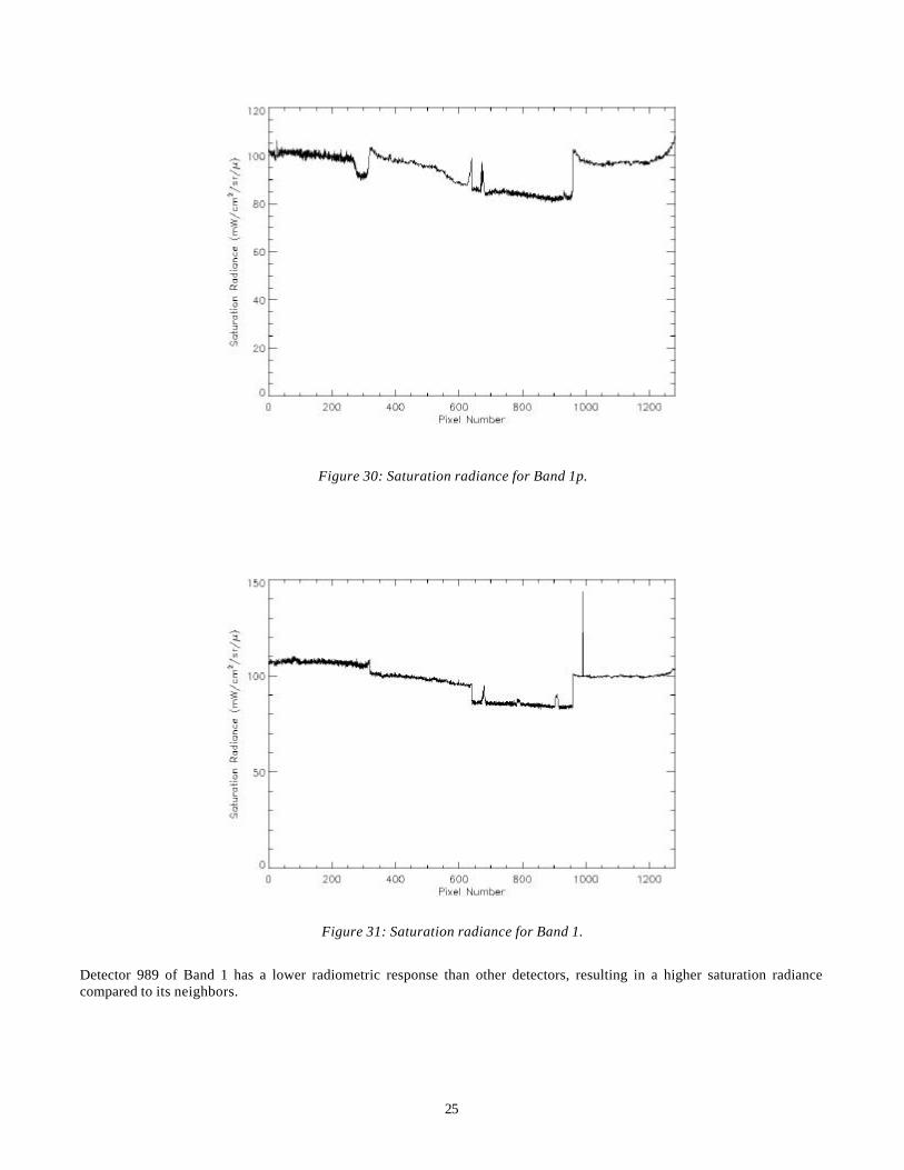
Figure 30: Saturation radiance for Band 1p.
Figure 31: Saturation radiance for Band 1.
Detector 989 of Band 1 has a lower radiometric response than other detectors, resulting in a higher saturation radiance compared to its neighbors.

26
Figure 32: Saturation radiance for Band 2.
Figure 33: Saturation radiance for Band 3.

27
Figure 34: Saturation radiance for Band 4.
Figure 35: Saturation radiance for Band 4p.

28
Figure 36: Saturation radiance for Band 5p.
Detectors 374 and 638 of Band 5p are inoperable detectors. The dip in saturation radiance, centered at detector 1200, is the result of an increase in dark current in this region of this band13. Detector 365 also has a larger than average dark current value.
Figure 37: Saturation radiance for Band 5.
29
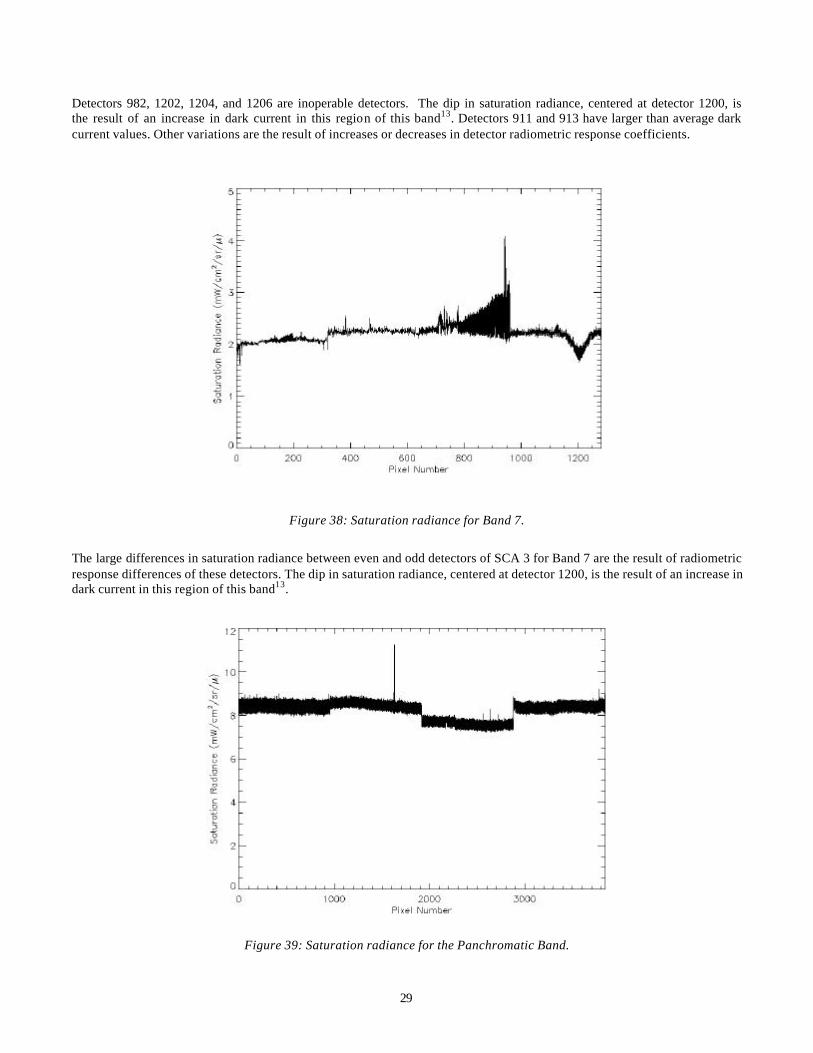
Detectors 982, 1202, 1204, and 1206 are inoperable detectors. The dip in saturation radiance, centered at detector 1200, is the result of an increase in dark current in this region of this band13. Detectors 911 and 913 have larger than average dark current values. Other variations are the result of increases or decreases in detector radiometric response coefficients.
Figure 38: Saturation radiance for Band 7.
The large differences in saturation radiance between even and odd detectors of SCA 3 for Band 7 are the result of radiometric response differences of these detectors. The dip in saturation radiance, centered at detector 1200, is the result of an increase in dark current in this region of this band13.
Figure 39: Saturation radiance for the Panchromatic Band.

30
Detector 1631 of the Panchromatic Band has a lower radiometric response relative to its neighbors, resulting in the observed saturation radiance increase. Dynamic Range The dynamic range of the ALI focal plane has been calculated as the ratio of the maximum dark current subtracted signal to the dark current noise
./)4095( PDarkP SPDR −=
Here, for detector P, DRP is the dynamic range, PDark is the dark offset, and SP is the noise for a dark scene (for these calculations, detector noises were assumed to be 1 DN)13. Adopting this method, the calculated dynamic range for the ALI focal plane is provided in Figures 40-49.
Figure 40: Dynamic range for Band 1p.
31
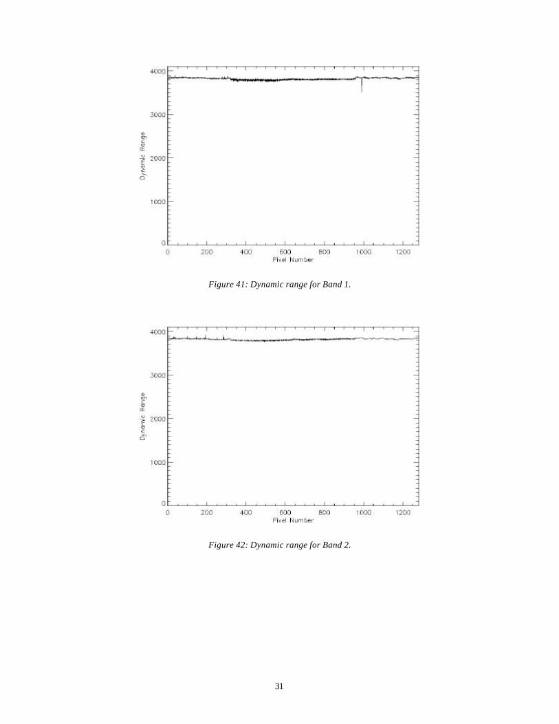
Figure 41: Dynamic range for Band 1.
Figure 42: Dynamic range for Band 2.

32
Figure 43: Dynamic range for Band 3.
Figure 44: Dynamic range for Band 4.
33
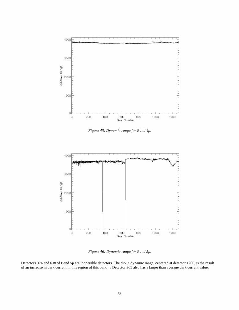
Figure 45: Dynamic range for Band 4p.
Figure 46: Dynamic range for Band 5p.
Detectors 374 and 638 of Band 5p are inoperable detectors. The dip in dynamic range, centered at detector 1200, is the result of an increase in dark current in this region of this band13. Detector 365 also has a larger than average dark current value.
34
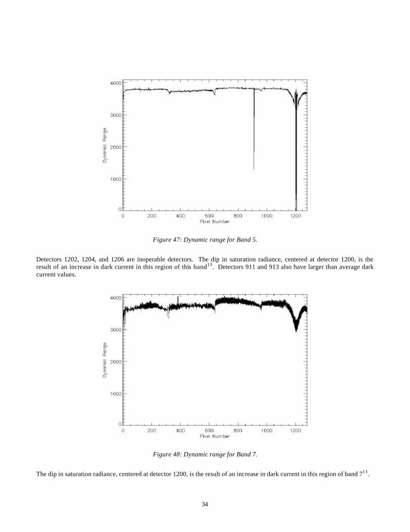
Figure 47: Dynamic range for Band 5.
Detectors 1202, 1204, and 1206 are inoperable detectors. The dip in saturation radiance, centered at detector 1200, is the result of an increase in dark current in this region of this band13. Detectors 911 and 913 also have larger than average dark current values.
Figure 48: Dynamic range for Band 7.
The dip in saturation radiance, centered at detector 1200, is the result of an increase in dark current in this region of band 713.

35
Figure 49: Dynamic range for the Panchromatic Band.

36
37
6. INTERNAL REFERENCE LAMPS
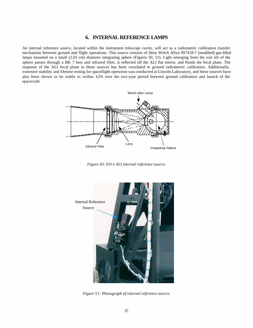
An internal reference source, located within the instrument telescope cavity, will act as a radiometric calibration transfer mechanism between ground and flight operations. This source consists of three Welch Allyn 997418-7 (modified) gas-filled lamps mounted on a small (2.03 cm) diameter integrating sphere (Figures 50, 51). Light emerging from the exit slit of the sphere passes through a BK 7 lens and infrared filter, is reflected off the ALI flat mirror, and floods the focal plane. The response of the ALI focal plane to these sources has been correlated to ground radiometric calibration. Additionally, extensive stability and lifetime testing for spaceflight operation was conducted at Lincoln Laboratory, and these sources have also been shown to be stable to within 1-2% over the two-year period between ground calibration and launch of the spacecraft.
Figure 50: EO-1 ALI internal reference source.
Figure 51: Photograph of internal reference source.
Integrat ing Sphere
Welch Allyn Lamp
LensInfrared Filter
Internal Reference
Source

38
Daily in-flight radiometric checks of the instrument will be conducted by observing these internal reference sources. Following each observation, after the aperture cover has been closed, the three internal reference lamps are powered by the ALI Control Electronics. After an eight-second stabilization period the lamps are sequentially powered down in a staircase fashion, with two-second exposures between each step. In this manner, the focal plane will receive a three point radiometric reference after each observation.

39
7. DISCUSSION
The radiometric response of the Earth Observing-1 Advanced Land Imager has been calibrated during ground testing at MIT Lincoln Laboratory. This calibration includes the investigation of the response, signal-to-noise ratio, saturation radiance, and dynamic range of each detector of every spectral band. The results obtained in the analysis outlined in this report, along with results from the leaky detector analysis, have been incorporated into the calibration pipeline and will be used to radiometrically calibrate initial ALI flight data. As an example of this calibration, Figure 52 depicts a Band 4 image of Lincoln Laboratory before and after radiometric calibration is applied. Detector-to-detector and SCA-to-SCA variations, a result of dark current and response coefficient variations, are clearly evident in the data prior to calibration.
Figure 52: Band 4 image of Lincoln Laboratory. The image on the left is prior to radiometric calibration. The image on the right is after radiometric calibration.
Finally, results presented here will also be compared against data collected during on-orbit internal reference lamp monitoring and solar, lunar, and vicarious calibrations to track changes in ALI radiometric response over the lifetime of the mission.

40

41
REFERENCES
1. J. A. Mendenhall et al., “Earth Observing-1 Advanced Land Imager: Instrument and Flight Operations Overview,” MIT/LL Project Report EO-1-1, 23 June 2000.
2. D. E. Lencioni, C. J. Digenis, W. E. Bicknell, D. R. Hearn, J. A. Mendenhall, “Design and Performance of the EO-1
Advanced Land Imager,” SPIE Conference on Sensors, Systems, and Next Generation Satellites III, Florence, Italy, 20 September 1999.
3. W. E. Bicknell, C. J. Digenis, S. E. Forman, D. E. Lencioni, “EO-1 Advanced Land Imager,” SPIE Conference on Earth
Observing Systems IV, Denver, Colorado, Proc. SPIE, Vol. 3750, pp. 80-88, 18 July 1999. 4. C. J. Digenis, D. E. Lencioni, and W. E. Bicknell, “New Millennium EO-1 Advanced Land Imager,” SPIE Conference
on Earth Observing Systems III, San Diego California, Proc. SPIE, Vol. 3439, pp. 49-55, July 1998. 5. D. E. Lencioni and D. R. Hearn, “New Millennium EO-1 Advanced Land Imager,” International Symposium on Spectral
Sensing Research, San Diego, Dec. 13-19, 1997. 6. “Landsat 7 System Specification,” Revision K, NASA Goddard Space Flight Center, 430-L-0002-K, July 1997. 7. J. A. Mendenhall and D. P. Ryan-Howard, “Earth Observing-1 Advanced Land Imager: Spectral Response Calibration,”
MIT/LL Project Report EO-1-2, 20 September 2000. 8. D. E. Lencioni, D. R. Hearn, J. A. Mendenhall, W. E. Bicknell, “EO-1 Advanced Land Imager Calibration and
Performance,” SPIE Conference on Earth Observing Systems IV, Denver, Colorado, Proc. SPIE, Vol. 3750, pp. 89-96, 18 July 1999.
9. J. A. Mendenhall, D. E. Lencioni, A. C. Parker, “Radiometric Calibration of the EO-1 Advanced Land Imager,” SPIE
Conference on Earth Observing Systems IV, Denver, Colorado, Proc. SPIE, Vol. 3750, pp. 117-131, 18 July 1999. 10. J. A. Mendenhall, D. E. Lencioni, D. R. Hearn, and A. C. Parker, “EO-1 Advanced Land Imager Preflight Calibration,”
Proc. SPIE, Vol. 3439, pp. 390-399, July 1998. 11. J. A. Mendenhall and D. E. Lencioni, “Earth Observing-1 Advanced Land Imager: Leaky Detector Calibration and
Correction,” MIT/LL Project Report, in preparation. 12. J. A. Mendenhall, “Earth Observing-1 Advanced Land Imager: Radiometric Response Calibration Addendum,” MIT/LL
Project Report, in preparation. 13. J. A. Mendenhall, “Earth Observing-1 Advanced Land Imager: Dark Current and Noise Characterization and Anomalous
Detectors,” MIT/LL Project Report, in preparation. ___________________________ This work was sponsored by NASA Goddard Space Flight Center under U.S. Air Force Contract F19628-00-C-0002. Opinions, interpretations, conclusions, and recommendations are those of the authors and are not necessarily endorsed by the United States Air Force.