Earth and Planetary Science Letters 304 (2011) 103–112

Contents lists available at ScienceDirect

Earth and Planetary Science Letters

j ourna l homepage: www.e lsev ie r.com/ locate /eps l

Rayleigh wave tomography of the northeastern margin of the Tibetan Plateau

Qie Zhang a,⁎,1, Eric Sandvol b, James Ni c, Yingjie Yang d, Yongshun John Chen e

a Exploration and Production Technology, BP America, Houston, TX 77079, USAb Department of Geological Sciences, University of Missouri, Columbia, MO 65211, USAc Department of Physics, New Mexico State University, Las Cruces, NM 88003, USAd Department of Physics, University of Colorado, Boulder, CO 80303, USAe Department of Geophysics, Peking University, Beijing 100871, PR China

⁎ Corresponding author.E-mail address: Qie.Zhang@bp.com (Q. Zhang).

1 Formerly: Department of Geological Sciences, Univer65211, USA.

0012-821X/$ – see front matter © 2011 Elsevier B.V. Adoi:10.1016/j.epsl.2011.01.021

a b s t r a c t

a r t i c l e i n f o

Article history:Received 22 April 2010Received in revised form 13 January 2011Accepted 23 January 2011Available online 26 February 2011

Editor: R.D. van der Hilst

Keywords:tomographyRayleigh wavesanisotropyTibet

The convergence between the Indian continent and the southern margin of Eurasia has eventually led to thegrowth of the Tibetan Plateau eastward. Various models have suggested that a large-scale flow in the lowercrust or/and the asthenosphere is responsible for the uplift of eastern Tibet. It has also been suggested that thecontinental flow may move around the thick lithosphere of the Ordos Plateau and the Sichuan Basin. In orderto investigate the validity of the crust/mantle flow and its possible path, we have used Rayleigh wavetomography with sensitivity kernels to estimate both the phase velocity structure (20–143 s) and the shearwave velocity structure (0–200 km) across the northeastern margin of the Tibetan Plateau. From the surfaceto 100 km, our shear wave velocity model shows a prominent low-velocity anomaly beneath northeasternTibet, suggestive of a warm lithosphere. Its boundary lies at ~105° E longitude which borders the westernOrdos Plateau and Sichuan Basin. From 125 km to 200 km, our shear wave velocity model shows a low-velocity channel beneath the Qilian–Qinling Orogen that lies between the Ordos and Sichuan blocks. Thischannel may represent the asthenosphere, given the fact that the lithosphere is ~120–150 km thick innortheastern Tibet and the Qinling Orogen. We also inverted for the anisotropy parameters in the study areasimultaneously with the velocity parameters. The dominant fast direction is NWW–SEE, generally consistentwith the SKS splitting results, the calculated shear-strain from GPS, and the fault slip rate measurements.Furthermore, the fast directions in our anisotropic model vary only slightly with periods and the anisotropymagnitudes at long periods (100–143 s) are large and exceed those at short–medium periods (20–80 s),indicating potentially (although not necessarily) vertically coherent deformation from the crust to theasthenosphere and possibly large deformation in the asthenosphere. The deformation seems to be linked tothe southeastward extrusion tectonics caused by the collision boundary force.

sity of Missouri, Columbia, MO

ll rights reserved.

© 2011 Elsevier B.V. All rights reserved.

1. Introduction

The Tibetan Plateau, the highest topography in the world, is theproduct of continent–continent collision between the Indian andEurasian plates that initiated ~50 Ma ago (e.g., Molnar and Tapponnier,1975; Yin and Harrison, 2000) (Fig. 1a). The collision not only causedsignificant elevation and highly deformed orogenic belts within theTibetan Plateau, butmay also impact remote areas such as eastern Chinaand the Baikal rift to the north (Bendick and Flesch, 2007; Molnar andTapponnier, 1975; Tapponnier andMolnar, 1977). Tibet is the onlywell-developed continental collision zone on Earth; hence, it attracts intensestudies, among which is the Inter-National Deep Profiling of Tibet andtheHimalaya (INDEPTH)project.While the previous three phases of the

INDEPTH project focused on the southern and central Tibetan Plateau(e.g., Brown et al., 1996; Tilmann et al., 2003; Zhao et al., 1993), ourrecent INDEPTH phase IV study (2007–2009) was designed toinvestigate the structure and evolution of the northeastern TibetanPlateau. As an integral part of the phase IV, we deployed 18 temporarybroadband stations (Fig. 1b) at the northeastern margin of the plateaufrom July 2008 to July 2009. The study area connects the margin of theTibetanPlateauwith theOrdosPlateauand theSichuanBasin (Fig. 1a, b).The latter twobelong respectively to theNorth Chinablock (apart of theSino–Korea craton) and the South China block (or the Yangtze craton),and are separated by the Qinling–Dabie orogenic belt. Our study area isstrategically located at this complex junction and new seismologicalobservations would help us better understand the geodynamics amongthose three major terrains in China.

The deformation of the Tibetan Plateau and its adjacent regions hasbeen explained by the extrusion tectonics: as the stronger Indian plateimpinged upon the Tibetan Plateau at a rate of ~5 cm/year, the forceled to the lateral escape of the plateau material towards the east andsoutheast along a series of strike–slip fault systems (e.g., Molnar and

Fig. 1. (a) Topographic relief of China and the location of our study area (white box).The study area (31°–38° N, 100°–109.5° E) is on the northeastern margin of the TibetanPlateau and includes the western Ordos Plateau and the northwestern Sichuan Basin(SB) that belong to the North China and the South China blocks, respectively. Bluearrows are the escaping directions of lower crust flow from Clark and Royden (2000).(b) Tectonic regions and the station distribution in our study area. White trianglesdenote 18 broadband seismic stations used in this study. The study area is also ourinversion area that expands out of the station-covered area. The red, purple, green andblue bars are the SKS shear wave splitting results from Wang et al. (2008), Chang et al.(2008), Huang et al. (2008), and our preliminary analysis (of INDEPTH IV stations),respectively. The green bars are mostly within the Weihe Graben (WG) that separatesthe Ordos Plateau from the Qinling Orogen.

104 Q. Zhang et al. / Earth and Planetary Science Letters 304 (2011) 103–112

Tapponnier, 1975; Tapponnier and Molnar, 1977). Tapponnier et al.(2001) consider the oblique crustal subduction/thrusting accommo-dated by the extrusion to be the mechanism of the growth and upliftof the eastern Tibetan Plateau. However, other scholars think that thelower crust flow is responsible for the high topography in the easternplateau (Clark and Royden, 2000; Clark et al., 2005; Royden et al.,1997, 2008). It has been hypothesized that when the crustal flowencounters the strong Ordos and Sichuan blocks, it changes directionsandmoves toward weaker regions. This deformational regime impliesa flow around the Sichuan Basin (Clark and Royden, 2000; Clark et al.,2005; Enkelmann et al., 2006; Royden et al., 2008) (Fig. 1a). Onebranch is thought to divert to the south of the Longmenshan Fault (thewestern boundary of the Sichuan Basin), and flow into the low land insouthwestern China (Li et al., 2009). The other branch seems to be

channeled eastward between the Ordos and Sichuan blocks along theQinling Orogen (Huang et al., 2008; Zhang et al., 1998). However, thetomographic evidences of the proposed flow paths remain unclear.

An important argument regarding the continental flow hypoth-esis is the depth and extent of its occurrence. Royden et al. proposethat the extrusion is detached from the upper crust and primarilyoccurs within the lower crust (Clark and Royden, 2000; Clark et al.,2005; Royden et al., 1997, 2008), considering the moderate amountof crustal shortening on the eastern plateau margin (Burchfiel et al.,1995). However, some studies (Flower et al., 1998; Huang et al.,2008; Liu et al., 2004) suggest that the extrusion may happenwidely in the asthenosphere. For example, Liu et al. (2004) imagedlow-velocity channels centered at a depth of ~250 km that connectwestern and eastern China using P wave tomography. If thecollision-driven lateral extrusion extends to the asthenosphericmantle and into eastern China, Huang et al. (2008) and Liu et al.(2004) believe that it could contribute to the widespread rifting andvolcanism in eastern China. Besides the opinions mentioned above,other researchers (Bendick and Flesch, 2007; Chang et al., 2008;Flesch et al., 2005; Wang et al., 2008) advocate vertically coupleddeformation between the crust and the lithospheric mantle basedon the agreement between the shear wave splitting data and thecalculated strain field from GPS and geological observations, butthey argue that the lithosphere instead of the asthenosphere is themajor source for the observed seismic anisotropy in the northeast-ern Tibetan Plateau.

To probe the lateral direction and depth extent of the potentialcontinental flow on the northeastern margin of the Tibetan Plateau,we investigated the 3-D velocity structure in this area usingRayleigh wave tomography of our new seismic dataset (from therecent INDEPTH IV deployment). Previous studies in northeasternTibet primarily focus on large-scale tomography (e.g., Huang andZhao, 2006; Li et al., 2008; Liang and Song, 2006; Liu et al., 2004;Pei et al., 2007; Su et al., 2008; Sun et al., 2008), and do not addressthe detailed velocity structure in our study area. Using the Rayleighsurface wave inversion with a sensitivity kernel technique thataccounts for finite frequency effects, we have computed both aphase velocity model and a shear wave velocity model in our studyregion. Shear wave velocities are sensitive to shear strength, so anyresolved low-velocity zone may help us understand the spatialdistribution of possible ductile flow channels in the crust or theasthenosphere. A simultaneous inversion resolving seismic anisot-ropy at different periods was also performed to give an estimate ofthe maximum strain directions as a function of depths.

2. Data collection and processing

We utilized fundamental mode Rayleigh waves from teleseismicevents for our study. The events were first selected using the criteriaof (1) magnitude Ms≥5.8 or Mb≥5.0, (2) epicenter distance between25° and 120°, and (3) depth≤100 km. We then carefully examinedeach individual event and eliminated those associated with low-quality waveforms (poor S/N ratios or inconsistent waveforms acrossthe seismic array). The process yielded a total of 74 good eventswhose locations are shown in Fig. 2a. The event azimuths are welldistributed, which can enhance resolving both lateral velocityheterogeneities and azimuthal anisotropy. The ray density is high(820–1000 rays) and the coverage is excellent for the periods of 40–143 s. The ray numbers decrease gradually to only a few hundredtowards the 20 s period. Fig. 2b–d shows the ray paths at the periodsof 25, 50, and 125 s in our study area. The dense crossing ray paths atmost periods are particularly suited for calculating the phase velocitystructure.

Among the 18 broadband stations in our study area (Fig. 1b), 17are equippedwith Streckeisen STS2 sensors. Only one station is with aGuralp CMG-3T sensor, and its instrument response was converted to

30°90°180°

100° 102° 104° 106° 108°

32°

34°

36°

38°

25 s (338 rays)

100° 102° 104° 106° 108°

32°

34°

36°

38°

50 s (967 rays)

100° 102° 104° 106° 108°

32°

34°

36°

38°

125 s (927 rays)

a b

c d

Fig. 2. (a) Locations of 74 teleseismic events (the circles) used to invert for the Rayleigh wave phase velocities. The star at the map center stands for our study area. Note that theevent azimuths are well distributed. (b–d) Great circle ray paths (gray lines) in our study area at the periods of 25, 50, and 125 s, respectively. The ray path coverage within thestation network (open triangles) is excellent for 50 and 125 s. Actually, every period in the range of 40–143 s has an excellent ray coverage with a large number of ray paths (820–1000 rays) (similar to those plotted in panels c and d).

105Q. Zhang et al. / Earth and Planetary Science Letters 304 (2011) 103–112

STS2 before the following processing. We have only used the verticalcomponent seismograms of Rayleigh waves to avoid the Love waveinterference and the long-period noise present on many of thehorizontal components. To measure their phase velocities at differentfrequency bands, we applied to the Rayleigh wave signals with 13band-pass filters that are 10-mHz-wide, zero-phase-shift Butterworthtype with center frequencies ranging from 7 to 50 mHz. Each filteredseismogram was visually checked to ensure that only high S/N ratioand coherent waveforms are retained. The signals of fundamentalmode Rayleigh waves were then isolated from noise and other phasesusing a boxcar window with cosine tapers at both ends. The windowlength is kept identical for all stations given any frequency–event pair.The phases and amplitudes of filtered and windowed Rayleigh waveswere measured by Fourier transform, and the measured amplitudeswere normalized for each event to eliminate the influence of theearthquake size.

Other than the energy focusing and defocusing caused bylateral velocity variations, two categories of major effects onRayleigh wave amplitudes need to be considered. The firstcategory includes geometric spreading, anelastic attenuation andlocal/station site responses that were corrected according to Yangand Forsyth (2006b). The other is the influence of scattering andmultipathing outside the array which is discussed in the followingsection.

3. Methodology

In our study, we used Yang and Forsyth's (2006a,b) method for theRayleigh wave tomographic inversion. The method has three mainfeatures: (1) using two-plane wave approximation to account forscattering and multipathing, (2) considering both amplitude andphase information, and (3) inverting based on 2-D sensitivity kernels.

Traditional teleseismic surface wave tomography assumes that theincoming wave travels along a great-circle path as a plane wave (dueto a large event-station distance). Normally, a two-station method isused to measure the phase differences and further calculate phasevelocities. However, lateral heterogeneities between the events andstations can produce strong scattering and multipathing, leading todistorted travel paths and non-planar wavefields. This phenomenoncan be observed from the amplitude variations (or interference)across the network (Forsyth and Li, 2005). Due to this factor,amplitude information is ignored in the traditional method. However,if it is possible to account for the scattering and multipathing effectsoutside the array which bias the phase velocity solutions within thearray, we can take advantage of both amplitude and phase measure-ments for the inversion. A two-plane wave technique (Forsyth and Li,2005; Li et al., 2003) helps compensate for the problem byapproximating the incoming wavefield with the sum/interference oftwo-plane waves. The technique provides stable solutions because it

3.2

3.4

3.6

3.8

4.0

4.2

4.4

Pha

se V

eloc

ity (

km/s

)

20 40 60 80 100 120 140

Period (s)

Fig. 3. Average Rayleigh wave phase velocities (solid line) in our study area at 13periods ranging from 20 to 143 s. This 1-D dispersion curve is used as an initial modelfor the inversions of 2-D phase velocity model (Fig. 4) and 1-D shear wave velocitymodel (solid line in Fig. 5). Error bars show the two standard deviations from the mean.The dashed line is the predicted phase velocity curve estimated from the 1-D shearwave velocities (solid line in Fig. 5). The predicted phase velocity curve matches theoriginal phase velocity curve, suggesting the dispersion curve and the shear wavevelocity curve fit each other very well. The dotted line shows the predicted phasevelocity curve estimated from the AK135 shear wave velocities. The predicted AK135phase velocities are higher than the resolved phase velocities in our study area at allperiods.

106 Q. Zhang et al. / Earth and Planetary Science Letters 304 (2011) 103–112

contains only 6 unknown wave parameters, that is, a pair ofamplitudes, phases and propagation directions, which are far fewerthan Friederich and Wielandt's (1995) approximation that uses a setof basis functions. The two-plane wave technique is tested to improvethe amplitude and phase misfits by ~30% over the one-plane wavetechnique (Li et al., 2003; Yang and Forsyth, 2006a), and it is widelyused for surfacewave tomographic studies (e.g., Forsyth et al., 1998; Liand Burke, 2006; Li et al., 2003; Yang and Forsyth, 2006b). Weadopted this two-plane wave technique for our study. Consideringthat the technique may not be suitable for modeling complexwavefields, we down-weighted the input waveform data accordingto their misfits and removed those with a poor match.

In conjunction with the two-plane wave technique, Yang andForsyth's (2006a) 2-D sensitivity kernel method was also utilized forour regional surface wave tomography. By taking the finite frequencyscattering effects into account, this sensitivity kernel method cantheoretically recover the anomalies close to the seismic wavelength(Yang and Forsyth, 2006a), which are not resolvable by using the raytheory. When complex structures such as strong crustal velocityvariations exist, the sensitivity kernel method is not easy to judgebecause the 2-D kernel functions used in the inversion could varyfrom the real ones (which are actually unknown). The sensitivitykernel function is derived from the single-scattering (Born) approx-imation (Zhou et al., 2004) and has an overall bell shape with its apexat the station. At a given frequency, it is a function of both thereference phase velocity and the isolation window used for dataprocessing. Here we omit the discussion on the theory and themathematical calculation of sensitivity kernels. Refer to Yang andForsyth (2006a,b) for the details.

Ignoring high-order terms, the surface wave phase velocity C in auniformly slightly anisotropic medium depends on both frequency ωand azimuth θ:

C ω; θð Þ = A0 ωð Þ + A1 ωð Þ cos 2θð Þ + A2 ωð Þ sin 2θð Þ; ð1Þ

where A0 is the azimuthally averaged phase velocity (i.e., isotropiccomponent), andA1 andA2 are azimuthal anisotropic coefficients (Smithand Dahlen, 1973). The phase delay δΦ and the relative amplitudevariation δlnA due to finite frequency scattering effects are defined as:

δϕ = ∬ΩKcΦ r;ωð Þ c−c0

c0

� �dxdy; ð2Þ

δlnA = ∬ΩKcA r;ωð Þ c−c0

c0

� �dxdy; ð3Þ

where (c−c0) is the phase velocity perturbation, c0 is the average phasevelocity, KΦ

c (r,ω) and KAc(r,ω) are 2-D phase and amplitude sensitivity

kernels, respectively, and the integration areaΩ is over the entire studyregion on the Earth surface.

We parameterized our study area with a total of 300 grid nodesand 0.5°×0.5° spacing. It is important to extend our nodes beyond thestation-covered area, so it allows the outer nodes to absorb somewavefield effects that are not completely described by two-planewaves. For the same purpose, a larger a priori error was assigned tothe edge nodes than the station-covered nodes during the inversion topermit less constrained solutions at the edge nodes. The phasevelocity at any point among the nodes in our study area is expressedby an interpolated value of the velocities at the surrounding nodesusing a 2-D Gaussian weighting function. The width Lw of theweighting function plays an important role in balancing thesmoothness and the resolution of the velocity model. Based on trial-and-error, we chose Lw to be 100 km. Other than the parameter Lw,two a priori variance values serving as damping terms were alsoassigned to each node in our inversion to control the solutions ofvelocity and anisotropy, respectively.

A two-stage inversion is adopted in our study to resolve theincoming wavefield parameters as well as the velocity (A0 in Eq. (1))and anisotropy (A1 and A2 in Eq. (1)) parameters at each grid nodeusing amplitude and phase data recorded at stations. For thefirst stage, the velocity model is fixed and only the wavefieldparameters are resolved by a simulated annealing method. In thesecond stage, all of the unknowns including wavefield parameters,velocity and anisotropy parameters, attenuation coefficients, and siteresponses are resolved based on a standard linear inversion method(Tarantola and Valette, 1982). Typically, the inversion processconverges within 10 iterations. More information regarding theinversion is provided by Forsyth and Li (2005) and Yang and Forsyth(2006a,b).

4. Results

4.1. 1-D phase velocity model

Before resolving 2-D phase velocity variations, we need to obtainan initial 1-D velocity model by inverting for the uniform phasevelocities in the entire study area. Fig. 3 shows the calculated averagedispersion curve at 13 periods that varies from 3.312 km/s at 20 s to4.218 km/s at 143 s. Because only one velocity model parameter isresolved for each period, the solutions are well constrained with verysmall standard deviations (0.004–0.008 km/s). The average disper-sion curve shows a consistent shape of concave downward. A slopechange at 33–50 s or ~40 s may correspond to the crust–mantletransition, where the surface wave sensitivity range shifts from bothcrust and mantle to mainly mantle.

4.2. 2-D phase velocity model

Using the above initial velocity model, we inverted for the lateralvariations of isotropic phase velocities (A0 in Eq. (1)) at each grid nodefor different periods. For the plotting purpose, we interpolated thephase velocities at finer grids (0.05°×0.05°) by using the sameGaussianweighting function (Lw=100 km). The interpolated velocitymaps are actually identical to those measured during the inversion.

107Q. Zhang et al. / Earth and Planetary Science Letters 304 (2011) 103–112

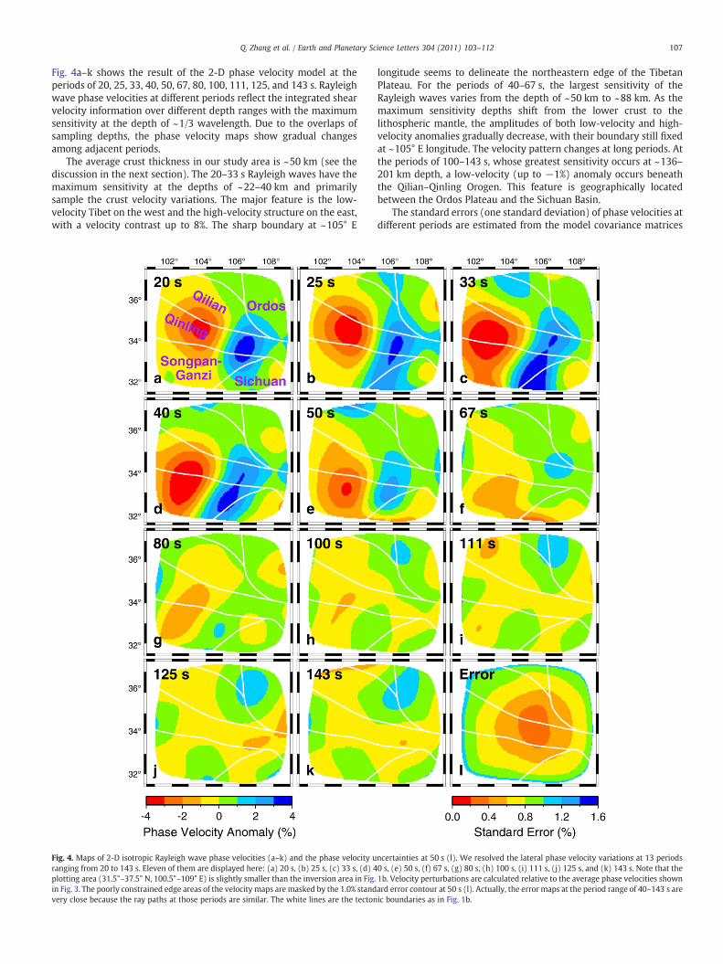
Fig. 4a–k shows the result of the 2-D phase velocity model at theperiods of 20, 25, 33, 40, 50, 67, 80, 100, 111, 125, and 143 s. Rayleighwave phase velocities at different periods reflect the integrated shearvelocity information over different depth ranges with the maximumsensitivity at the depth of ~1/3 wavelength. Due to the overlaps ofsampling depths, the phase velocity maps show gradual changesamong adjacent periods.

The average crust thickness in our study area is ~50 km (see thediscussion in the next section). The 20–33 s Rayleigh waves have themaximum sensitivity at the depths of ~22–40 km and primarilysample the crust velocity variations. The major feature is the low-velocity Tibet on the west and the high-velocity structure on the east,with a velocity contrast up to 8%. The sharp boundary at ~105° E

Fig. 4. Maps of 2-D isotropic Rayleigh wave phase velocities (a–k) and the phase velocity uranging from 20 to 143 s. Eleven of them are displayed here: (a) 20 s, (b) 25 s, (c) 33 s, (d) 4plotting area (31.5°–37.5° N, 100.5°–109° E) is slightly smaller than the inversion area in Fig.in Fig. 3. The poorly constrained edge areas of the velocity maps are masked by the 1.0% standvery close because the ray paths at those periods are similar. The white lines are the tecton

longitude seems to delineate the northeastern edge of the TibetanPlateau. For the periods of 40–67 s, the largest sensitivity of theRayleigh waves varies from the depth of ~50 km to ~88 km. As themaximum sensitivity depths shift from the lower crust to thelithospheric mantle, the amplitudes of both low-velocity and high-velocity anomalies gradually decrease, with their boundary still fixedat ~105° E longitude. The velocity pattern changes at long periods. Atthe periods of 100–143 s, whose greatest sensitivity occurs at ~136–201 km depth, a low-velocity (up to −1%) anomaly occurs beneaththe Qilian–Qinling Orogen. This feature is geographically locatedbetween the Ordos Plateau and the Sichuan Basin.

The standard errors (one standard deviation) of phase velocities atdifferent periods are estimated from the model covariance matrices

ncertainties at 50 s (l). We resolved the lateral phase velocity variations at 13 periods0 s, (e) 50 s, (f) 67 s, (g) 80 s, (h) 100 s, (i) 111 s, (j) 125 s, and (k) 143 s. Note that the1b. Velocity perturbations are calculated relative to the average phase velocities shownard error contour at 50 s (l). Actually, the error maps at the period range of 40–143 s areic boundaries as in Fig. 1b.

300

250

200

150

100

50

0

Dep

th (

km)

3.0 3.5 4.0 4.5 5.0

S wave Velocity (km/s)

Fig. 5. Average shear wave velocities (solid line) in our study area. This model isobtained by inverting average phase velocities in Fig. 3 with the crust thickness fixed at50 km. The starting model for the inversion is a slightly modified AK135 velocity model(dashed line). The resolved 1-D shear wave velocities are lower than the AK135reference velocities. Our resolved 1-D model is then adopted as an initial model for the3-D inversion of shear wave velocities (Fig. 6).

108 Q. Zhang et al. / Earth and Planetary Science Letters 304 (2011) 103–112

and the weighting function. All of these standard error maps share asimilar pattern with error values increasing from the center (station-covered area) to the edge of the study area. An example of onestandard errormap at 50 s period is shown in Fig. 4l. The errormaps atthe periods of 40–143 s are very much comparable, because of thesimilar ray paths and ray numbers at those periods (Fig. 2b–d). The1.0% error contour in Fig. 4l is used to mask the poorly constrainededges of those 2-D phase velocity models (Fig. 4a–k). A checkerboardresolution test at 50 s is also performed and the result is plotted in thesection of auxiliary materials. The alternating high and low velocitiesare resolved reasonably well which confirms the reliability of ourphase velocity model.

4.3. 1-D shear wave velocity model

For the purpose of geological interpretation, we converted the phasevelocities to the shear wave velocities, so the velocity information for agiven depth range can be isolated. Other than top a few tens ofkilometers (e.g., crustal structure), Rayleigh wave phase velocitiesdepend mainly on S wave velocities, instead of P wave velocities anddensity. Therefore, we can assume a constant Poisson's ratio and onlyinvert for the S wave velocity structure. During the inversion, Saito's(1988) algorithm is used to calculate the partial derivatives of phasevelocities with respect to the model parameters (i.e., P and S wavevelocities) and the synthetic phase velocities that best fit the observedphase data. Because the inversion process is non-linear and under-determined, we assigned a priori constraints, that is, a correlationcoefficient and a standard deviation value to the diagonal and off-diagonal components of the model covariance matrix, respectively, toallow damping and vertical smoothing during the inversion. Theaverage shear wave velocity model in our study area is first resolvedto serve as an initial model for the next step of 3-D inversion.

Due to the large tradeoff between the Moho depth and the seismicvelocity structure adjacent to the Moho discontinuity, we took the apriori information of crust thickness for our 1-D inversion. Receiverfunction studies (Duan et al., 2007; Li et al., 2006b; Lou et al., 2009; Tonget al., 2007) suggest an averageMoho depth at ~50 km in our study area(Fig. 6i). Li et al.'s (2006b) stations cover a large part of our central studyarea with the Moho depths varying from 44 km to 56 km. Duan et al.'s(2007) receiver function analysis on aN–S arrayof 22 stations at ~103° Elongitude yields an approximately flat Moho at 50 km. Tong et al.'s(2007) 13-station array across the southwestern edge of the OrdosPlateau produces close crust thickness values (49–55 km) with a meanof 52 km. Lou et al.'s (2009) study shows that the Moho depths changefrom 40 km in the western Sichuan Basin to 56 km in the Songpan–Ganzi terrain. Other than the receiver function results, deep seismicsounding profiles in China (Li et al., 2006a) suggest ~50 km of theaverage Moho depth in our study area as well. Therefore, we fixed thecrust thickness at 50 km for our 1-D shear wave velocity inversion. Weslightly modified the AK135 shear wave velocity model (Kennett et al.,1995) to create our 1-D initial shear wave velocity model whichprimarily contains 25-km-thick layers. During the inversion,we allowedthe 1-D velocities to vary down to 410 km, but here we only plotted theresolved velocity curve down to 300 km and we do not interpret thevelocity structure deeper than 250 km because the maximum sensitivedepth obtained from our dispersion data is ~201 km (corresponding tothe maximum period of 143 s). The result is shown in Fig. 5, where wecan see the resolved average shearwave velocities are all lower than thereference AK135 model down to 250 km. Low velocities in the uppermantle suggest that high temperature or potential partialmelting in themantle may occur widely in our study area.

4.4. 3-D shear wave velocity model

For each map point in our study area, we inverted independently forits 1-D shearwave velocities from its dispersion curve using the previous

1-D inversion method (Section 4.3). The 1-D shear wave velocities at allmappointswere then gathered to construct our 3-D shearwave velocitymodel. During the inversion, the shear wave velocities are fixed below200 kmwhere Rayleigh wave data do not have a sufficient resolution todetermine the lateral velocity variations reliably. The initial shear wavevelocitymodel for themappoint inversion is our optimal 1-Dshearwavevelocity model (solid line in Fig. 5) with its crust thickness correctedaccording to the interpolated/extrapolated Moho depths from receiverfunctionanalyses (Duanet al., 2007; Li et al., 2006b; Louet al., 2009; Tonget al., 2007) (Fig. 6i). The corrected Moho depths vary from 40 km to56 km in our study area, and the upper crust thickness is defined to be ahalf of the Moho depth. Again, both upper and lower crust thicknessesare fixed during the map point inversion.

It is important to note that the Moho depths vary dramatically andabruptly in our study area (Fig. 6i), and the resolved shearwave velocitystructure adjacent to theMohodiscontinuity is highly dependent on thecrust thickness values specified in the initial model. Due to the limitedconstraints from the available receiver function data, the resolved smallvelocity anomalies around the Moho could be artifacts due to potentialerrors in our a priori crust thickness map. Therefore, for the upper100 km of our resolved velocity model, we only interpreted the first-order features (detailed small anomalies are probably not reliable).However, the choiceofMohodepthmaphas little impact onourvelocitystructure deeper than 100 km. We have tested our 3-D shear wavevelocity model by using two additional Moho depth maps, i.e., Li et al.'s(2006a)Mohomap aswell as aflat 50 kmMohomap (the currentMohomap is from combined receiver function results as shown in Fig. 6i), andfound that the resolved structures beneath 100 km are very close to ourcurrent resolved image in Fig. 6.

The results of 3-D shear wave velocities are shown in Fig. 6a–hwith a similar pattern to our phase velocity maps (Fig. 4a–k). For thedepths of 0–100 km, the first-order feature of the shear wave velocitymodel is still the low-velocity (up to −4%) northeastern TibetanPlateau and the high-velocity (up to 3%) region that lies outside theplateau. The major difference between the phase and shear wavevelocity models is the high-velocity anomaly shifted eastwards in thelatter model (it will be explained in Section 5). For the depths of 125–200 km, the shear wave velocity model indicates a low-velocity (up to−1%) channel beneath the Qilian–Qinling Orogen that lies betweenthe Ordos and Sichuan blocks, similar to our phase velocity model.

Fig. 6. Maps of 3-D isotropic shear wave velocities (a -h) and Moho depths (i) in our study area. Velocity perturbations are calculated relative to the average shear velocities (solidline in Fig. 5). The 3-D shear wave velocity model is constructed by inverting the dispersion curve at eachmap point. The shear wave velocities at 0–200 km are resolved with the restfixed during the inversion. The initial model for the inversion is adopted from Fig. 5 with the Moho depth corrected according to the receiver function results (i). Panel (a) layer(upper crust) is from the surface to half of theMoho depth. Panel (b) layer (lower crust) is from half of the Moho depth to theMoho depth. Panel (i) shows theMoho depths from thereceiver function analyses. Red, green, blue and purple triangles stand for the stations from Tong et al. (2007), Duan et al. (2007), Li et al. (2006b) and Lou et al. (2009), respectively.The adjacent numbers are Moho depths in kilometers.

109Q. Zhang et al. / Earth and Planetary Science Letters 304 (2011) 103–112

Since our average shear wave velocities at 125–200 km are 1–1.5%lower than those of the global AK135 model (Fig. 5), the low-velocityregion is probably up to 2.5% lower than the global average velocity.

4.5. 1-D anisotropy model

Unlike shear wave splitting measurements characterized by apoor vertical resolution, the anisotropy analysis using surface wavesprovides valuable vertical information because surface waves aresensitive to different depth ranges at different periods. To find theazimuthal anisotropy features of Rayleighwaves at those 13 periods inour study area, we performed another inversion simultaneouslyresolving the velocity coefficient A0 and the anisotropy coefficientsA1 and A2 in Eq. (1). The percentage of anisotropy magnitude (thevelocity difference between the fast and slow directions dividedby the isotropic velocity) is then measured by the formula

2ffiffiffiffiffiffiffiffiffiffiffiffiffiffiffiffiffiffiffiffiffiffiffiffiffiffiffiffiffiffiffiffiffiffiffiffiffiffiA1ðωÞ2 + A2ðωÞ2

q= A0ðωÞ. The fast direction (anisotropic azimuth)

at a particular frequency is the θ value that maximizes the phasevelocity C(ω,θ) in Eq. (1). By setting the derivative ∂C(ω,θ)/∂θ=0,

two potential solutions (θ = 12 tan

−1ðA2ðωÞ= A1ðωÞÞ or 12 tan

−1ðA2ðωÞ=A1ðωÞÞ + π

2) are derived. When plugged back in Eq. (1), only onesolution maximizes C(ω,θ) and is the final answer of fast anisotropicdirection. The other solution is corresponding to the smallest C(ω,θ) andtherefore the slowest directionwhich is always perpendicular to the fastdirection for the velocity expressed in Eq. (1). Standard deviations of themagnitude and the fast direction can be further estimated from thevariances of A1 and A2 using an error propagation technique (Clifford,1975). Although anisotropy terms are introduced, the resolved velocityimage is very close to the result (Section 4.2 and Fig. 4) after theinversionwith only isotropic terms. The fact is probably due to the evenazimuthal coverage of our ray paths.

Theoretically, azimuthal anisotropy can be resolved at each gridnode, but this nearly triples the number of unknowns during theinversion that can cause instability in our solutions. Considering thesmall number of stations in our seismic array, we only inverted for theuniform azimuthal anisotropy (that varies only with periods) in ourwhole study area. The result (Fig. 7) shows a consistent NWW–SEE fastdirection for all the periods and increasing anisotropy amplitudes from~1% at 22–80 s to ~3% at 100–143 s. The inversion of the fast directions

0

1

2

3

4

Ani

sotr

opy

(%)

20 40 60 80 100 120 140

Period (s)

N

Avg SKS dir

Avg strain dir

Fig. 7. Variations of average azimuthal anisotropy with periods in the whole study area.The result was resolved by assuming uniform anisotropy in the whole study area thatvaries only with periods. For each period, the percentage of anisotropy magnitude isrepresented by the vertical axis, and the fast direction of azimuthal anisotropy isrepresented by the orientation of a slanted black bar as in a map view with Northpointing up. One standard deviation of the anisotropy magnitude and the fast directionare depicted by a pair of vertical and slanted gray bars, respectively. Inserted are theaverage SKS fast direction (from Fig. 1b) and the average maximum shear straindirection (from Fig. 6 in Flesch et al., 2005) in our study area. They both show a NWW–

SEE direction which agrees with our anisotropic orientation.

110 Q. Zhang et al. / Earth and Planetary Science Letters 304 (2011) 103–112

seems to be well constrained because their error bounds are small. Oursurface wave anisotropy is in a good agreement with surfacedeformation data (Flesch et al., 2005; Wang et al., 2008) and SKSsplitting observations (Chang et al., 2008;Huanget al., 2008;Wanget al.,2008)whose fast directions are primarily between E–WandNW–SE too(Fig. 1b). Our fast direction is also roughly parallel to the low-velocitychannel beneath theQinlingOrogen imaged in our phase velocitymodel.

5. Discussion

Bothour phase velocitymodel (Fig. 4) andshearwave velocitymodel(Fig. 6) reveal significant anomalies within our study area. The patternsof the velocity variations fall into two categories: (1) short periods (20–67 s) or 0–100 km, and (2) long periods (100–143 s) or 125–200 km.Since the lithosphere thickness beneath the northeastern TibetanPlateau and the Qinling Orogen is ~120–150 km (An and Shi, 2006),the vertical change of the velocity patterns in our study area is probablyrelated to the transition from the lithosphere to the asthenosphere.

The phase velocitymaps at the periods of 20–67 s (Fig. 4a–f) show aprominent low-velocity (up to −4%) anomaly beneath the northeast-ern Tibetan Plateau with a boundary at ~105° E longitude. The samelow-velocity (up to −4%) zone also appears in the shear wave velocitymaps from the surface to 100 km (Fig. 6a–d). The northeastern TibetanPlateau is dominated by highly deformed orogenic belts and fold zones(the Qilian Orogen, the Qinling Orogen, and the Songpan–Ganzi foldzone), and the associated low-velocity anomaly may present weak andwarm crust and uppermost mantle. A few deformational mechanismsincluding lower crustal flow (Clark and Royden, 2000; Clark et al., 2005;Royden et al., 1997, 2008) and vertically coherent lithosphericdeformation (Chang et al., 2008; Flesch et al., 2005; Silver, 1996;Wang et al., 2008) have also been proposed to occur broadly in thislow-velocity area. On the other hand, our eastern study area showsoverall fast velocities in the lithosphere (0–100 km). The phase velocitymaps at the periods of 20–67 s (Fig. 4a–f) image the highest-velocity(up to 4%) anomaly adjacent to the boundary of northeastern Tibet (i.e.,west of the Longmenshan Fault and the southwestern edge of the OrdosPlateau). This high-velocity anomaly seems to be a result of theshallowest Moho depth (see receiver function results in Fig. 6i) in ourstudy area, as a shallower Moho normally brings both the crust andmantle velocities near the Moho higher. As a consequence of the crustthickness variation, this highest-velocity anomaly also becomes less

pronounced and shifts eastwards (Fig. 6a–d) during the conversionfrom the phase velocities to the shear wave velocities where the crustthickness is taken into account. Our eastern study area includes thewestern portions of the Ordos Plateau and the Sichuan Basin which areold and stable Archean cratonic blocks. Many other seismic tomo-graphic studies suggest that these two blocks are featured by high-velocity lithospheric roots (e.g., Huang and Zhao, 2006; Li et al., 2008,2009; Liang and Song, 2006; Pei et al., 2007; Su et al., 2008; Sun et al.,2008), however, our data do not image these two blocks very well dueto our limited station coverage (Fig. 1b) and insufficient Moho depthconstraint (Fig. 6i). The major reliable feature in our lithosphericvelocity models is the first-order velocity boundary at ~105° Elongitude that is likely to be the eastern edge of the Tibetan Plateau.

The phase velocity pattern at long periods (100–143 s) (Fig. 4h–k)varies from that at short periods (20–67 s) (Fig. 4a–f). The long periodmaps show a low-velocity (up to −1%) channel beneath the Qilian–Qinling Orogen that connects northeastern Tibet to eastern China. Thischannel is observed in our shear wave velocity model as well with asimilar shape that spans the depths of 125–200 km (Fig. 6f–h).Roughly bounded by the Ordos Plateau and the Sichuan Basin, thelow-velocity channel probably represents the asthenosphere beneaththe Qilian Orogen, which agrees with An and Shi's (2006) estimationof lithospheric thickness. Although our tomography does not providea sufficient resolution below 200 km, other large-scale P wavetomographic studies (Huang and Zhao, 2006; Li et al., 2008; Liuet al., 2004) show that the low-velocity channel is present at 200–300 km and may continue beyond 300 km. A very likely explanationof this low-velocity channel is the eastward flow of mantle material inthe asthenosphere caused by the collision between the Indian andEurasian plates, and seismic anisotropy data can further helpconstrain the idea.

Our fast shear wave direction derived from Rayleigh wavetomography in the whole study area is NWW–SEE and varies littlewith periods (Fig. 7). This is consistent with a vertically similardeformation field (from the surface to 200 km) in our study area, ifmantle anisotropy is assumed to be a result of lattice preferredorientation in olivine and follows the maximum shear direction (forsimple shear) or extensional direction (for pure shear). Our fastpolarization direction generally agrees with those results: thepredicted shear-strain from GPS and Quaternary fault slip ratemeasurements (which are surface deformation data that can beconsidered a proxy for the upper crustal deformation) (Flesch et al.,2005; Wang et al., 2008), the SKS splitting analyses (which estimatethe accumulative shear wave anisotropy along the ray path from thecore–mantle boundary to the surface) (Chang et al., 2008; Huang etal., 2008; Wang et al., 2008), and another Rayleigh wave anisotropystudy (Su et al., 2008). According to Silver's (1996) annual reviewpaper, two major mechanisms account for the mantle deformationbeneath continents: (1) simple asthenospheric flow, and (2) verticallycoherent deformation. The former mechanism assumes the astheno-spheric mantle to be kinematically decoupled from the overridinglithosphere and dominate the mantle anisotropy. Our anisotropy datado not support different deformation regimes between the litho-sphere and the asthenosphere, and Flesch et al.'s (2005) numericalmodeling test of “simple asthenospheric flow” in northern Tibet is alsounsuccessful. On the contrary, the latter mechanism is consideredas “fossilized” lithospheric deformation produced primarily by thelast significant tectonic event. In this case, the crust and the sub-continental mantle deform as a coherent unit, and the surfacegeology/deformation data match the mantle anisotropy measure-ments. Silver (1996) considers northern Tibet to be a remarkableexample for the “vertically coherent deformation” mechanism,because the spatial SKS splitting parameters consistently track themodern orogeny (both mantle shortening and extrusion). Based onthe tests of a few scenarios, Flesch et al. (2005) also conclude that amodel of strongly coupled crust and lithospheric mantle with

111Q. Zhang et al. / Earth and Planetary Science Letters 304 (2011) 103–112

vertically coherent deformation dominated in the Tibetan lithospherebest fits the surface deformation and mantle anisotropy data (thestudy also explains why maximum shear instead of maximumextension is a better predictor for the mantle anisotropy). Thismodel precludes the hypothesis of a large-scale lower crust flow(a “jelly-sandwich” model) (Clark and Royden, 2000; Clark et al.,2005; Royden et al., 1997) where the upper crust and the uppermantle are completely decoupled. Our consistent anisotropy directionat different depths (Fig. 7) and its agreement with surface deforma-tion and SKS splitting data (Fig. 7) seem to favor the model ofvertically coherent deformation, although our anisotropic result itselfcan not completely exclude the existence of a mechanically weak zonebetween the crust and the mantle.

Different theories have been proposed regarding the depth extentof the deformation field in the Tibetan Plateau. Royden et al. (Clarkand Royden, 2000; Clark et al., 2005; Royden et al., 1997) believe thatthe ductile flow is primarily confined within the lower crust, butFlesch et al. (2005) and Wang et al. (2008) suggest that thedeformation is dominant in the lithosphere other than in theasthenosphere. Nonetheless, our anisotropy model shows a differentstory. Significant anisotropic strength (~2.7%) appears at the periodsof 100–143 s, larger than that at short periods (Fig. 7). These longperiods correspond to the asthenospheric depth range in northeasternTibet (see the earlier discussion), so our anisotropy data can probablyinfer the presence of large deformational fabrics in the asthenosphericmantle. Silver (1996) also thinks that the mantle deformation of Tibetcan extend down to 300 km based on a large SKS delay estimate(2.4 s) near Kunlun fault. Furthermore, as plotted in Fig. 1b, Huanget al.'s (2008) and Chang et al.'s (2008) shear wave splitting analysesrecord a few large delay times (≥1.4 s and ≥0.8 s, respectively).Those large delays also seem to require a substantial contributionfrom the asthenosphere, given the lithosphere thickness (b150 km) innortheastern Tibet and the Qinling Orogen (Huang et al., 2008).

In our anisotropic model, the fast velocities in the asthenosphere(long periods) and the lithosphere (short periods) share a commonNWW–SEE direction. The direction is roughly parallel to the low-velocity channel (likely to be the asthenosphere) beneath the QinlingOrogen imaged in our velocity models. Therefore, the fast direction orthe possible deformational orientation may indicate a ductile flow inthe asthenosphere in the Qinling Orogen between the Ordos Plateauand the Sichuan Basin. As a collision boundary and a left-lateral strikeslip fault zone between the North China and South China blocks, theQinling Orogen could provide a channel to direct the eastward flow ofthe extruded material caused by the India–Eurasia collision. We alsopropose that the collision boundary force is the major source for thevertically consistent deformation field (0–200 km) in our study area,because it could provide a consistent driving force over a large rangeof depth and cause vertically coherent deformation, regardless ofrheology or decoupled zones (Flesch et al., 2005). The gravity forcemay also contribute to the deformation in our study area, but morerequirements are needed to produce vertically coherent deformation(Flesch et al., 2005).

6. Conclusions

We have used Rayleigh wave tomography with a two-plane waveapproach and a sensitivity kernel inversion to image the velocity andanisotropy structures beneath the northeastern Tibetan Plateau. Ourphase velocity and shear wave velocity models both indicate that thelithosphere (0–100 km) in our study area can be divided into the low-velocity (weak lithosphere) northeastern Tibetan Plateau and thehigh-velocity eastern study area with a sharp boundary at ~105° Elongitude. On the other hand, in the asthenosphere (125–200 km), weobserve a low-velocity zone beneath the Qilian–Qinling Orogen thatlies between the Ordos Plateau and the Sichuan Basin. This zone mayact as a channel directing the asthenospheric flow eastwards. Our

anisotropymodel of thewhole study area shows a uniformNWW–SEEfast direction for all the periods (20–143 s), which agrees with SKSsplitting observations and surface deformation data. The verticalconsistency of different measurements of the deformational fieldseems to support that the deformation may occur coherently from thecrust to the asthenosphere in our study area. Our anisotropy modelalso shows a significant amount of anisotropy at long periods (100–143 s), indicating large deformation in the asthenosphere. We suggestthat the ductile flow induced by the compression between the Indianand Asian plates occurs down to the asthenosphere and probablywraps around the rigid Sichuan Basin. The collision boundary forceseems to account for the vertically coherent deformation due to itstransmission ability throughout a large-scale depth range.

Acknowledgements

We appreciate IRIS and PASSCAL's support of the deployment ofthe INDEPTH-IV/ASCENT array. This work is supported by theContinental Dynamics program at the National Science Foundation,Grant nos. EAR0409589 and EAR0409870.

Appendix A. Supplementary data

Supplementary data to this article can be found online atdoi:10.1016/j.epsl.2011.01.021.

References

An, M.J., Shi, Y.L., 2006. Lithospheric thickness of the Chinese continent. Phys. EarthPlanet. In. 159, 257–266. doi:10.1016/j.pepi.2006.08.002.

Bendick, R., Flesch, L., 2007. Reconciling lithospheric deformation and lower crustalflow beneath central Tibet. Geology 35, 895–898. doi:10.1130/G23714A.1.

Brown, L.D., Zhao, W.J., Nelson, K.D., Hauck, M., Alsdorf, D., Ross, A., Cogan, M., Clark, M.,Liu, X.W., Che, J.K., 1996. Bright spots, structure, and magmatism in Southern Tibetfrom INDEPTH seismic reflection profiling. Science 274, 1688–1691.

Burchfiel, B.C., Chen, Z.L., Liu, Y.P., Royden, L.H., 1995. Tectonics of the Longmen Shanand adjacent regions, Central China. Int. Geol. Rev. 37, 661–735.

Chang, L.J., Wang, C.Y., Ding, Z.F., 2008. Seismic anisotropy of upper mantle in Sichuanand adjacent regions. Sci. China, Ser. D Earth Sci. 51, 1683–1693.

Clark, M.K., Royden, L.H., 2000. Topographic ooze: building the eastern margin of Tibetby lower crustal flow. Geology 28, 703–706.

Clark, M.K., Bush, J., Royden, L., 2005. Dynamic topography produced by lower crustalflow against rheological strength heterogeneities bordering the Tibetan Plateau.Geophys. J. Int. 162, 575–590.

Clifford, A.A., 1975. Multivariate Error Analysis. John Wiley, Hoboken, N. J.Duan, Y.H., Zhang, X.K., Liu, Z., Xu, Z.F., Wang, F.Y., Pan, J.S., Liang, G.J., 2007. Crustal

structure using receiver function in the east part of Anyemaqen suture belt? ActaSeismol. Sin. 20, 513–522.

Enkelmann, E., Ratschbacher, L., Jonckheere, R., Nestler, R., Fleischer, M., Gloaguen, R.,Hacker, B.R., Zhang, Y.Q., Ma, Y.S., 2006. Cenozoic exhumation and deformation ofnortheastern Tibet and the Qinling: is Tibetan lower crustal flow diverging aroundthe Sichuan Basin? Geol. Soc. Am. 118, 651–671. doi:10.1130/B25805.1.

Flesch, L.M., Holt, W.E., Silver, P.G., Stephenson, M., Wang, C.Y., Chan, W.W., 2005.Constraining the extent of crust–mantle coupling in central Asia using GPS,geologic, and shear wave splitting data. Earth Planet. Sci. Lett. 238, 248–268.doi:10.1016/j.epsl.2005.06.023.

Flower, M., Tamaki, K., Hoang, N., 1998. Mantle extrusion: a model for dispersedvolcanism and DUPAL-like asthenosphere in East Asia and the western Pacific. In:Flower, M.F.J., Chung, S.-L., Lo, C.-H., Lee, T.-Y. (Eds.), Mantle Dynamics and PlateInteractions in East Asia, Geodynamics Series. American Geophysical Union,Washington, DC, pp. 67–88.

Forsyth, D.W., Li, A., 2005. Array analysis of two-dimensional variations in surface wavephase velocity and azimuthal anisotropy in the presence of multipathinginterference. In: Levander, A., Nolet, G. (Eds.), SeismicEarth: Array Analysis ofBroadband Seismograms. : Geophys. Monogr. Ser., 157. AGU, Washington, D. C, pp.81–97.

Forsyth, D.W.,Webb, S., Dorman, L., Shen, Y., 1998. Phase velocities of Rayleigh waves inthe MELT experiment on the East Pacific Rise. Science 280, 1235–1238.

Friederich, W., Wielandt, E., 1995. Interpretation of seismic surface waves in regionalnetworks: joint estimation of wavefield geometry and local phase velocity. Methodand tests. Geophys. J. Int. 120, 731–744.

Huang, J., Zhao, D., 2006. High-resolution mantle tomography of China and surroundingregions. J. Geophys. Res. 111, B09305. doi:10.1029/2005JB004066.

Huang, Z., Xu, M., Wang, L., Mi, N., Yu, D., Li, H., 2008. Shear wave splitting in thesouthern margin of the Ordos Block, north China. Geophys. Res. Lett. 35, L19301.doi:10.1029/2008GL035188.

Kennett, B.L.N., Engdahl, E.R., Buland, R., 1995. Constraints on seismic velocities in theEarth from travel times. Geophys. J. Int. 122, 108–124.

112 Q. Zhang et al. / Earth and Planetary Science Letters 304 (2011) 103–112

Li, A., Burke, K., 2006. Upper mantle structure of southern Africa from Rayleigh wavetomography. J. Geophys. Res. 111, B10303. doi:10.1029/2006JB004321.

Li, A., Forsyth, D.W., Fischer, K.M., 2003. Shear velocity structure and azimuthalanisotropy beneath eastern North America from Rayleigh wave inversion. J.Geophys. Res. 108 (B8), 2362. doi:10.1029/2002JB002259.

Li, S.L., Mooney, W.D., Fan, J.C., 2006a. Crustal structure of mainland China from deepseismic sounding data. Tectonophysics 420, 239–252.

Li, Y.H., Wu, Q.J., An, Z.H., Tian, X.B., Zeng, R.S., Zhang, R.Q., Li, H.G., 2006b. The Poissonratio and crustal structure across the NE Tibetan Plateau determined from receiverfunctions. Chin. J. Geophys. (in Chinese) 49, 1359–1368.

Li, C., van der Hilst, R.D., Meltzer, A.S., Engdahl, E.R., 2008. Subduction of the Indianlithosphere beneath the Tibetan Plateau and Burma. Earth Planet. Sci. Lett. 277,157–168.

Li, H.Y., Su,W.,Wang, C.Y., Huang, Z.X., 2009. Ambient noise Rayleigh wave tomographyin western Sichuan and eastern Tibet. Earth Planet. Sci. Lett. 282, 201–211.doi:10.1016/j.epsl.2009.03.021.

Liang, C.T., Song, X.D., 2006. A low velocity belt beneath northern and eastern TibetanPlateau from Pn tomography. Geophys. Res. Lett. 33, L22306. doi:10.1029/2006GL027926.

Liu, M., Cui, X.J., Liu, F.T., 2004. Cenozoic rifting and volcanism in eastern China: amantle dynamic link to the Indo–Asian collision? Tectonophysics 393, 29–42.

Lou, H., Wang, C.Y., Lu, Z.Y., Yao, Z.X., Dai, S.G., You, H.C., 2009. Deep tectonic setting ofthe 2008 Wenchuan Ms8.0 earthquake in southwestern China — joint analysis ofteleseismic P-wave receiver functions and Bouguer gravity anomalies. Sci. China,Ser. D Earth Sci. 52, 166–179.

Molnar, P., Tapponnier, P., 1975. Cenozoic tectonics of Asia: effects of a continentalcollision. Science 189, 419–426.

Pei, S.P., Zhao, J.M., Sun, Y.S., Xu, Z.H.,Wang, S.Y., Liu, H.B., Rowe, C.A., Toksoz, M.N., Gao, X.,2007. Upper mantle seismic velocities and anisotropy in China determined throughPn and Sn tomography. J. Geophys. Res. 112, B05312. doi:10.1029/2006JB004409.

Royden, L.H., Burchfiel, B.C., King, R.W., Wang, E., Chen, Z.L., Shen, F., Liu, Y.P., 1997.Surface deformation and lower crustal flow in eastern Tibet. Science 276, 788–790.

Royden, L.H., Burchfiel, B.C., van der Hilst, R.D., 2008. The geological evolution of theTibetan Plateau. Science 321, 1054–1058.

Saito, M., 1988. DISPER80: a subroutine package for the calculation of seismic normal-mode solutions. In: Doornbos, D.J. (Ed.), Seismological Algorithms. Elsevier, NewYork, pp. 293–319.

Silver, P.G., 1996. Seismic anisotropy beneath the continents: probing the depths ofgeology. Annu. Rev. Earth Planet. Sci. 24, 385–432.

Smith, M.L., Dahlen, F.A., 1973. The azimuthal dependence of Love and Rayleigh wavepropagation in a slightly anisotropic medium. J. Geophys. Res. 78, 3321–3333.

Su, W., Wang, C.Y., Huang, Z.X., 2008. Azimuthal anisotropy of Rayleigh waves beneaththe Tibetan Plateau and adjacent areas. Sci. China, Ser. D Earth Sci. 51, 1717–1725.

Sun, Y.S., Toksoz, M.N., Pei, S.P., Zhao, D.P., Morgan, F.D., Rosca, A., 2008. S wavetomography of the crust and uppermost mantle in China. J. Geophys. Res. 113,B11307. doi:10.1029/2008JB005836.

Tapponnier, P., Molnar, P., 1977. Active faulting and tectonics in China. J. Geophys. Res.82, 2905–2930.

Tapponnier, P., Xu, Z., Roger, F., Meyer, B., Arnaud, N., Wittlinger, G., Yang, J., 2001.Oblique stepwise rise and growth of the Tibet Plateau. Science 294, 1671–1677.

Tarantola, A., Valette, B., 1982. Generalized non-linear problems solved using the least-squares criterion. Rev. Geophys. 20, 219–232.

Tilmann, F., Ni, J., INDEPTH III Team, 2003. Seismic imaging of the downwelling Indianlithosphere beneath central Tibet. Science 300, 1424–1427. doi:10.1126/sci-ence.1082777.

Tong, W.W.,Wang, L.S., Mi, N., Xu, M.J., Li, H., Yu, D.Y., Li, C., Liu, S.W., Liu, M., Sandvol, E.,2007. Receiver function analysis for seismic structure of the crust and uppermostmantle in the Liupanshan area, China. Sci. China, Ser. D Earth Sci. 50, 227–233.

Wang, C.Y., Flesch, L.M., Silver, P.G., Chang, L.J., Chan, W.W., 2008. Evidence formechanically coupled lithosphere in central Asia and resulting implications.Geology 36, 363–366. doi:10.1130/G24450A.1.

Yang, Y.J., Forsyth, D.W., 2006a. Regional tomographic inversion of the amplitude andphase of Rayleighwaveswith 2-D sensitivity kernels. Geophys. J. Int. 166, 1148–1160.

Yang, Y.J., Forsyth, D.W., 2006b. Rayleigh wave phase velocities, small-scale convection,and azimuthal anisotropy beneath southern California. J. Geophys. Res. 111,B07306. doi:10.1029/2005JB004180.

Yin, A., Harrison, T.M., 2000. Geologic evolution of the Himalayan–Tibetan orogen.Annu. Rev. Earth Planet. Sci. 28, 211–280.

Zhang, Y.Q., Mercier, J.L., Vergely, P., 1998. Extension in the graben systems around theOrdos (China), and its contribution to the extrusion tectonics of south China withrespect to Gobi-Mongolia. Tectonophysics 285, 41–75. doi:10.1016/S0040-1951(97)00170-4.

Zhao, W., Nelson, K.D., Project INDEPTH, 1993. Deep seismic reflection evidence forcontinental underthrusting beneath southern Tibet. Nature 366, 557–559.

Zhou, Y., Dahlen, F.A., Nolet, G., 2004. Three-dimensional sensitivity kernels for surfacewave observables. Geophys. J. Int. 158, 142–168.