Earnings Mobility and Measurement Error:A Pseudo-Panel Approach∗

Francisca Antman Department of Economics, Stanford University

David J. Mckenzie† Development Research Group, The World Bank

Revised December 12, 2006

Abstract

The degree of mobility in incomes is often seen as an important measure of the equality of opportunityin a society and of the flexibility and freedom of its labor market. However, estimation of mobility usingpanel data is biased by the presence of measurement error and non-random attrition from the panel.This paper shows that dynamic pseudo-panel methods can be used to consistently estimate measuresof absolute and conditional mobility when genuine panels are not available, and in the presence of non-classical measurement errors. These methods are applied to data on earnings from a Mexican quarterlyrotating panel. Absolute mobility in earnings is found to be very low in Mexico, suggesting that the highlevel of inequality found in the cross-section will persist over time. However, the paper finds conditionalmobility to be high, so that households are able to recover quickly from earnings shocks. These findingssuggest a role for policies which address underlying inequalities in earnings opportunities.

JEL classification: O12, D31, C81Keywords: income mobility, dynamic pseudo panel; measurement error.

∗We thank the Stanford Center for International Development (SCID) for research funding; and John Strauss, an associateeditor, two referees, Aart Kraay and participants at the PACDEC and LACEA conferences for helpful comments.

†Corresponding Author: Development Research Group, World Bank, MSN MC3-300, 1818 H Street N.W., Washington D.C.20433; Email: dmckenzie@worldbank.org; Phone: (202) 458-9332; Fax: (202) 522-3518.

1

1 Introduction

The degree of mobility in income is often seen as a measure of the equality of opportunity in a society, and of

the flexibility and freedom of movement in the labor market (Atkinson, Bourguignon and Morrisson, 1992).

Depending on the mobility process, greater mobility may lead to more equally distributed lifetime incomes

for a given level of single period income inequality. On the other hand, Jarvis and Jenkins (1998) note that

too much mobility may represent income fluctuations and economic insecurity. Gottschalk and Spolaore

(2002) formalize this trade-off in a model with both aversion to inequality and aversion to unpredictability of

incomes, finding the socially desirable level of mobility will be less than a level at which there is full reversal

of ranks over time. Nevertheless, in many developing countries, the concern is more likely to be that there

is too little, rather than too much, mobility. In particular, Piketty (2000) surveys recent theoretical work

which finds that the presence of credit constraints can give rise to the possibility of “low-mobility traps”,

whereby households who need to borrow to finance investment can take a long time to build up wealth.

Measurement of the degree of mobility using panel data on earnings is complicated by the presence of

measurement error, and by non-random attrition from the panel. A simple measure of mobility is the slope

coefficient from a regression of current period earnings on lagged earnings (e.g. Jarvis and Jenkins, 1998;

Fields et al. (2003)).1 Classical measurement error causes the well-known attenuation bias towards zero in

the estimated slope coefficient, leading one to overstate the degree of mobility. Dragoset and Fields (2006)

estimate mobility regressions with survey data and administrative data, and find quantitatively less conver-

gence with the administrative data. The existing literature has attempted to overcome the measurement

error problem through the use of instrumental variable methods. Instruments for lagged income have in-

cluded lagged expenditure (e.g. McCulloch and Baulch, 2000), subjective measures of well-being (Luttmer,

2002)2, assets and land holdings (e.g. Fields et al. (2003), Strauss et al. (2004)), and weight (Glewwe and

Nguyen, 2002).However, we show that instrumental variables will only be consistent if the instrument is not

only uncorrelated with the measurement error but also has the same amount of mobility as earnings. This

condition appears extremely unlikely to hold in practice.

The literature has devoted less attention to assessing the impact of attrition on estimates of mobility.

However, the typical labor force panel in developing countries reinterviews dwelling units, rather than house-

holds, so that households that move attrit from the sample. The Mexican Urban Labor Force Survey (ENEU)

used in this study is a quarterly rotating panel which follows this approach, and on average loses 35 percent

of the sample due to attrition over the five periods. Thomas, Frankenberg and Smith (2001) discuss the

experience of the Indonesia Family Life Survey, which explicitly tracked movers, and do find that those who

move are different in terms of initial characteristics than those who stay. Although they do not examine

whether changes in income or other economic conditions are associated with households being more likely to

1See Fields and Ok (1999) for a review of other concepts of mobility.2Luttmer actually examines mobility in expenditure, rather than income, and uses income and subjective well-being as

instruments for expenditure.

2

move, one would expect greater geographic mobility to be associated with more income mobility: households

experiencing large positive shocks may move to better housing while households experienced large negative

shocks may migrate or move to cheaper housing. As a result, the attrition bias may lead panel studies to

understate mobility.

This paper shows how dynamic pseudo-panel methods can be used to consistently estimate the degree

of income mobility when earnings contain non-classical measurement error, also allowing for mobility mea-

surement when panel data are not available. A pseudo-panel tracks cohorts of individuals over repeated

cross-sectional surveys (Deaton, 1985). Intuitively, the use of a pseudo-panel helps deal with measurement

error in two ways. Firstly, construction of a pseudo-panel involves taking cohort means within each time

period, and this averaging process eliminates individual-level measurement error in the cross-section. Sec-

ondly, since each household is only observed once, the measurement errors observed in one period will be

for different households than the measurement errors observed in another period. Non-random attrition also

becomes much less of an issue since each household need only be observed once. Repeated cross-sectional

surveys are available in more countries and typically over longer time-periods than genuine panels. This

allows one to estimate mobility measures over many more time periods than typically used in the panel

literature. Gottschalk (1997) notes that many movements in income are transitory, so that individuals who

experience an increase in earnings in one year will tend to have a fall in income a few years later. Therefore

mobility over several periods may be different from what one would predict based on extrapolating measures

based on a one year interval.

This paper uses 58 quarters of household earnings data in Mexico over the period 1987 to 2001 to

examine earnings mobility. Mexico’s income distribution displays a high degree of cross-sectional inequality,

and therefore a high degree of income mobility is of importance in lowering inequality in lifetime distributions

of income. However, our pseudo-panel results find very low levels of absolute mobility in Mexico. While OLS

estimation would suggest that 33 percent of the gap in income between two randomly selected households

would close within one quarter, pseudo-panel analysis finds only 1.2 percent of this gap would be eliminated

within a quarter, and only five to seven percent of income differences disappear after five years. In contrast,

while absolute mobility remains low, conditional mobility, defined as the movement in income around a

household’s fixed effect, is found to be quite rapid. Households which experience bad luck or shocks to labor

earnings which take them below the level of income determined by their individual attributes recover almost

fully to their expected level within two years. These findings of slow absolute mobility and rapid conditional

mobility continue to hold using full income and expenditure from an alternate dataset. As a result, the high

levels of inequality seen in a given cross-section are likely to persist over time.

Two recent papers by Duval-Hernández (2006) and Fields et al. (2006) also use the same labor income

data as used here to investigate mobility and earnings dynamics in Mexico. Using a series of panels of two

observations one year apart, they study how mobility varies over time, during recessions and recoveries,

and with individual characteristics. To control for measurement error, they relate the change in earnings to

3

predicted earnings, thereby focusing on how mobility relates to longer-term measures of income. In findings

similar to ours, Duval-Hernández (2006) finds a high degree of convergence to conditional mean earnings,

but little convergence in terms of absolute earnings. While we differ in approach, allowing for individual

fixed effects and longer-term dynamics, it is reassuring to see an approach somewhat similar in spirit achieve

similar results qualitatively.

The remainder of the paper is structured as follows. Section 2 discusses estimation of mobility by OLS

and IV in the presence of non-classical measurement errors. Section 3 shows how pseudo-panel estimation

can allow for consistent estimation. Section 4 provides Monte-Carlo evidence. Section 5 describes the data.

Section 6 contains the main results of the paper while Section 7 provides an interpretation of the findings.

Section 8 concludes.

2 Mobility and Measurement Error

While there are many potential measures of mobility (see Atkinson et al. (1992)), we investigate one of the

simplest measures, which is the slope coefficient in a regression of income on its lagged value. This measure

is common in much of the empirical literature (e.g. Jarvis and Jenkins, 1998; Fields et al. (2003); Strauss

et al. (2004)). Moreover, because this measure is based on a regression framework, pseudo-panel methods

and instrumental variables can be applied to deal with measurement error.

Consider the data generating process for the actual log income, Y ∗i,t of individual i at time period t:

Y ∗i,t = α+ βY ∗i,t−1 + ui,t (1)

The coefficient β is a measure of (im)mobility. A value of β of unity indicates that incomes move in step,

with no convergence of incomes. If β is greater than unity, there is divergence, and β less than one indicates

some convergence of incomes. Gottschalk and Spolaore (2002) consider two aspects of economic mobility.

‘Origin independence’ measures the degree to which future incomes do not depend on present income. β

equal to zero combined with no individual fixed effects in the error term, ui,t would indicate full original

independence. They also consider a second aspect, ‘reversal’, which is the degree to which ranks are reversed

over time. A value of β less than zero would indicate some reversal, with individuals with above mean

income experiencing a fall in income and poorer individuals getting richer. The socially optimal level of β

will involve a trade-off between the degree of aversion to inequality (which favors lower values of β) and

the degree of aversion to unpredictability of income (which favors values of β closer to one). Consistent

measurement of β is needed to assess the degree of mobility.

However, in practice data are measured with error. One thus observes:

Yi,t = Y ∗i,t + εi,t (2)

The degree of bias in mobility estimates arising from measurement error, and the ability of different tech-

niques to correct for this bias depend critically on the assumptions one makes about εi,t. Several validation

4

studies from the United States have found that the measurement error in incomes is unlikely to be classi-

cal.3 In particular, Bound and Krueger (1991) compare the Current Population Survey to Social Security

Administrative records in the United States and find that the measurement error in earnings is positively

autocorrelated over two years, and is negatively correlated with true earnings. There are a number of reasons

to expect measurement error to be greater in developing country settings, for which validation data are not

available. In particular, levels of literacy are lower, deliberate misreporting to avoid taxes may be greater,

and more of the workforce tends to be employed in informal work and in self-employment. In our data, 27

percent of workers are in self-employment, while over half the workforce is not registered with the Mexican

social security system. Only 24 percent of firms in the 1998 Mexican Microenterprise Survey (ENAMIN)

keep formal records, and 57 percent keep no records at all. Measurement error is highly likely to be larger

in these firms than for wage workers in the U.S.

Our pseudo-panel estimation below can allow for very general forms of measurement error at the individual

level. In particular, we can allow εi,t to be autocorrelated and correlated with Y ∗i,t and/or ui,t. However,

certain types of measurement error may also be correlated across individuals. One part of the error may be

due to enumerator bias, so that different individuals surveyed by the same enumerator will have correlated

measurement errors. Likewise, similar characteristics across households within an area may also cause

all households within an area to have correlated measurement errors. Our pseudo-panel estimator will be

consistent if there is weak spatial correlation between observations, such as that considered by Chang (2002).4

Our identifying assumption is therefore that a law of large numbers applies within a cohort, so that as the

number of individuals within a cohort, nc →∞

1

nc

ncXi=1

εi,tp→ 0 (3)

This assumption is quite weak and covers a large number of cases which violate the assumption of classical

measurement error. However, it will be violated if all individuals within a cohort have a common time-varying

component to their measurement error. We therefore proceed on the assumption that equation (3) holds,

and return to examining the performance of our estimator under violations of this assumption in Section 4.

Substituting (2) into (1) gives the equation to be estimated in terms of observed income:

Yi,t = α+ βYi,t−1 + ηi,t (4)

where ηi,t = ui,t + εi,t − βεi,t−1 (5)

Consider the OLS estimator of β based on equation (4):

bβOLS =NPi=1

Yi,tyi,t−1

NPi=1

Yi,t−1yi,t−1

3Bound et al. (2001) provide a comprehensive review.4For example, assume that within a cohort for each t, ε(t) = (ε1,t, ..., εnc,t) is an i.i.d. (0,Σ) sequence of random variables

with E ε(t)4<∞. The matrix Σ should be non-singular, but need not be diagonal.

5

where yi,t−1 = Yi,t−1 − (1/N)PN

i=1 Yi,t−1. One can then show under standard assumptions that as the

number of observations in the cross-section, N , goes to infinity,

bβOLS p→ β + θOLS

where θOLS = [Cov (ui,t, Yi,t−1) + Cov (εi,t, εi,t−1) + Cov¡εi,t, Y

∗i,t−1

¢−βV ar (εi,t−1)− βCov

¡Y ∗i,t−1, εi,t−1

¢]/V ar (Yi,t−1) (6)

The term θOLS is the asymptotic bias and shows that OLS will be inconsistent in general. This inconsistency

arises due to the following terms:

i) Cov (ui,t, Yi,t−1), the covariance between the current period shock to earnings and last period’s mea-

sured earnings. The standard concern here is the presence of individual fixed effects in the error term

ui,t, which will lead to this term being positive. This term will also not be zero if earnings shocks, ui,t

are autocorrelated.

ii) Cov (εi,t, εi,t−1) , the covariance between this period’s and last period’s measurement error terms will

be non-zero if measurement errors are autocorrelated. Based on the U.S. validation studies, we would

expect this term to be positive.

iii) Cov¡Y ∗i,t−1, εi,t−1

¢, the covariance between the measurement error and true earnings. The results of

Bound and Krueger (1991) suggest this term will be negative. In addition, if the measurement errors

are positively autocorrelated, then the covariance between last period’s true earnings and the current

period’s measurement error, Cov¡εi,t, Y

∗i,t−1

¢, may also be negative.

iv) V ar (εi,t−1), the variance of the measurement error. If there are no fixed effects, and the measurement

error is classical, then we have: bβOLS p→ β

∙1− V ar (εi,t−1)

V ar (Yi,t−1)

¸(7)

This is the classic attenuation bias towards zero, and would lead one to conclude there is more mobility

in income than there actually is.

2.1 Instrumental Variables

In recognition of the effect of measurement error on mobility estimates, several authors have attempted to use

instrumental variables methods. As discussed in the introduction, instruments used for income have included

education, expenditure, asset holdings, and weight. Let Zi,t−1 be the instrument. Then it is assumed that

the actual data are related to the instrument according to:

Y ∗i,t−1 = φ+ γZi,t−1 + vi,t−1 (8)

Where γ 6= 0 is a necessary condition for instrument relevance. Writing this in terms of the observed Yi,t−1

then gives the first-stage equation:

Yi,t−1 = φ+ γZi,t−1 + vi,t−1 + εi,t−1 (9)

6

Let zi,t−1 = Zi,t−1 − (1/N)PN

i=1 Zi,t−1 denote the demeaned Zi,t−1. The instrumental variables estimator

of β based on equation (9) being used as a first-stage for Yi,t−1 in equation (4) is then:

bβIV =

NPi=1

Yi,tzi,t−1

NPi=1

Yi,t−1zi,t−1

= β +

NPi=1

(ui,t + εi,t − βεi,t−1) zi,t−1

NPi=1

Yi,t−1zi,t−1

(10)

In order to determine the probability limit of this estimator, we need to impose some structure on the time

series properties of the instrument. Let us assume that:

Zi,t = μ+ ρZi,t−1 + ωi,t (11)

This formulation allows us to vary the degree of autocorrelation in the instrument by varying ρ, and to also

consider the case of time invariant instruments such as education, for which ρ = 0 and ωi,t = ωi. Appendix

1 then shows that as N →∞,

bβIV p→ β +γ (ρ− β)V ar (Zi,t−1) +E (εi,tZi,t−1)− βE (εi,t−1Zi,t−1) + λ

γV ar (Zi,t−1) +E (Zi,t−1εi,t−1)(12)

where

λ = γE (ωi,tZi,t−1) +E (vi,tZi,t−1) (13)

Equation (12) thus shows that consistency of the instrumental variables estimator requires that all of the

following conditions hold:5

1. The instrument Zi,t−1 is uncorrelated with both the current and lagged measurement errors. This

appears unlikely to hold when using expenditure as an instrument for income, but appears plausible

for measures such as education and body weight.

2. λ = 0. This requires that the instrument, Zi,t−1 be uncorrelated with the error terms ωi,t and vi,t.

This condition will be violated if the true data, Y ∗i,t contain individual fixed effects which are correlated

with the instrument, or if the dynamic process governing the evolution of the instrument itself contains

an individual fixed effect. Again, this restriction appears problematic when using expenditure as an

instrument for income, since one might expect individual fixed effects in income and expenditure to be

correlated.

3. The degree of autocorrelation in the instrument must perfectly match the degree of autocorrelation in

income, that is, ρ = β. This condition is unlikely to be met by many of the instruments used in the

5Of course it is theoretically possible that the bias terms could cancel one another out, so that we could obtain consistency

without the separate bias terms all being zero, but this appears unlikely in practice.

7

literature. In particular, there is no reason to expect the degree of autocorrelation in asset holdings or

in body weight to be the same as in earnings. Note that if conditions 1 and 2 hold, then

bβIV p→ ρ (14)

That is, the instrumental variables estimator will converge to the autocorrelation coefficient in the

instrument. Hence, if one uses an instrument which does not vary over time, such as education of

adults, then ρ = 1, and bβIV will converge to unity.6 If one uses an instrument which is white noise,

then bβIV will converge to zero.These three conditions are unlikely to be met simultaneously by most of the candidate instruments used

thusfar in the literature. Instruments such as repeated measures of income are most likely to display the same

degree of autocorrelation as true earnings, but also therefore likely to have correlated measurement errors

and also potentially have individual fixed effects correlated with those in genuine earnings. Instruments such

as body weight, education, and land holdings are less likely to have measurement errors correlated with the

measurement error in earnings, but also be less likely to display identical dynamics to income. As a result,

the above analysis suggests that all such IV estimators will deliver inconsistent estimates of mobility.

2.2 Instrumental Variables with Individual Effects

It is common practice in dynamic panel data estimation to worry about the presence of individual fixed

effects. As seen above, even when there is no measurement error, the presence of individual fixed effects

can result in inconsistent estimates of β from both OLS and from certain instrumental variable estimators.

The standard solution is to difference the data and then use further lags of income as an instrument. As

our panels are very short, we will follow Arellano (1989) in using Yi,t−2 as an instrument for ∆Yi,t−1. The

Arellano instrumental variables estimator is then:

βA =

NPi=1(∆Yi,t)Yi,t−2

NPi=1(∆Yi,t−1)Yi,t−2

(15)

Assume that after removing individual fixed effects, the ui,t are not autocorrelated and are independent of

Y ∗i,s for s < t, and are independent of the measurement error. Then if the measurement error is classical,

one can show that as N →∞,

βAp→ β

Ã1− V ar (εi,t−2)

(1− β)E¡Y 2i,t−2

¢+ βV ar (εi,t−2)

!(16)

Therefore with classical measurement error, the Arellano instrumental variables estimator will be biased

towards zero for 0 < β < 1. The presence of measurement error will therefore lead this estimator to

6Glewwe and Nyugen (2002) also show that the correlation coefficient between current and lagged income will be unity in

their IV method when using an instrument which does not vary over time.

8

overstate the degree of mobility.7

3 Pseudo-panel Estimation

We propose using pseudo-panel methods to consistently estimate the degree of income mobility in the presence

of measurement error. A pseudo-panel tracks cohorts of individuals, such as birth cohorts, or birth-education

cohorts, over repeated cross-sectional surveys. Since a new sample of individuals is taken in each period,

the use of a pseudo-panel will also greatly reduce the effect of attrition on mobility estimates. The use of

the pseudo-panel will capture mobility which is accompanied by movement within the cross-sectional survey

domain. However, it will not capture mobility which arises from migration into or out of the survey area.

Moffitt (1993), Collado (1997), McKenzie (2001a, 2004) and Verbeek and Vella (2005) discuss conditions

under which one can consistently estimate linear dynamic models with pseudo-panels. Our aim here is to

show that these methods can also deal with the measurement error problems facing panel data models.

Begin by taking cohort averages of equation (4) over the nc individuals observed in cohort c at time t :

Y c(t),t = α+ βY c(t),t−1 +

uc(t),t + εc(t),t − βεc(t),t−1 (17)

where Y c(t),t = (1/nc)Pnc

i=1 Yi(t),t denotes the sample mean of Y over the individuals in cohort c observed

at time t. With repeated cross-sections, different individuals are observed each time period. As a result, the

lagged mean Y c(t),t−1, representing the mean income in period t− 1 of the individuals in cohort c observedat time t, is not observed. Therefore we replace the unobserved terms with the sample means over the

individuals who are observed at time t− 1, leading to the following regression for cohorts c = 1, 2, ..., C and

time periods t = 2, ..., T :

Y c(t),t = α+ βY c(t−1),t−1 +

uc(t),t + εc(t),t − βεc(t),t−1 + λc(t),t (18)

where

λc(t),t = β¡Y c(t),t−1 − Y c(t−1),t−1

¢As shown in McKenzie (2004), as the number of individuals in each cohort becomes large, λc(t),t converges

to zero, and hence we will ignore this term in what follows.8 However, note that this assumption does require

that individuals with the same mean incomes at time t− 1 be surveyed at time t and time t+1. This posesa problem when using a pseudo-panel for older cohorts, where, for example, poorer individuals may be more

likely to die between time t and t + 1 than richer individuals. It can also pose a problem for very young7Again if we allow for non-classical measurement error the bias term becomes more complicated and theoretically difficult

to sign.8This additional measurement error term introduced by the use of pseudo-panel analysis does not affect consistency of

estimation, but does change the standard error (see McKenzie (2004) for details).

9

age groups, who may be in the process of forming households. Similarly, if a large number of individuals

migrate between periods, this can also cause this assumption to be violated. This issue is less likely to be a

problem if one looks over shorter time periods, such as the quarterly surveys used here, and concentrates on

prime-aged household heads, such as the 25 to 49 year olds we use. However, it does make the method less

suitable for looking at mobility early or late in life.9

Consider then the mean measurement error in income at time t for individuals in cohort c, εc(t),t. As the

number of individuals in the cohort gets large, nc →∞, we have that under the assumption in equation (3):

εc(t),t =1

nc

ncXi=1

εi(t),tp→ 0

This assumes that there is no cohort-level component to measurement errors. We can allow for cohort-

specific effects in equation (18), in which case we need only assume that there is no time-varying cohort-level

component to measurement errors.

This assumption does allow for arbitrary autocorrelation in individual measurement errors over time,

for measurement errors to be correlated with true values, and for weak spatial correlation. Under these

assumptions, construction of the pseudo-panel, by averaging over the observations in a cohort, will average

out the measurement errors. Note also that any dynamics in individual measurement errors will not cause

inconsistency, since we observe different individuals each period. As a result, with sufficient observations per

cohort, the measurement errors do not affect the consistency of estimates from equation (18). Although the

pseudo-panel estimator will be consistent under the assumptions given, note that the speed of convergence

depends on the number of individuals per cohort, nc, rather than on the total number of individuals in the

sample. Thus the standard errors from pseudo-panel estimation will be larger than those obtained with

genuine panels.

The precise method for estimating equation (18) depends on the assumptions one wishes to make about

the individual level shocks to earnings, ui,t, and on the dimensions of the pseudo-panel in practice. McKenzie

(2004) discusses these choices. In particular, if the ui,t contain individual fixed effects but no time-varying

cohort-level component, one can estimate β consistently by OLS on the cohort average equation (18) with

the inclusion of cohort dummies. This will be consistent as the number of individuals per cohort gets large.

If the individual level shocks to earnings contain a common cohort component, then in addition to a large

number of individuals per cohort, one also needs a large number of cohorts or a large number of time periods

for consistency. With many cohorts and less individuals per cohort, instrumental variables methods can be

used in which lagged cohort means are used as instruments (see Collado, 1997). In our empirical context

we choose cohorts to allow for a large number of individuals per cohort, and therefore can use OLS on the

cohort means for estimation.9Bounds analysis can be used to determine the impact of changes in the composition of a cohort over its life cycle on the

validity of estimates, see, e.g. McKenzie (2001b).

10

3.1 Mobility and heterogeneity

The most basic specification is therefore to assume that there are no individual fixed effects, in which case

one uses the pseudo-panel to estimate β in the following equation:

Y c(t),t = α+ βY c(t−1),t−1 + ωc(t),t (19)

If Y is the level of income, then β < 1 then tells us that a household with income below the mean in

period t − 1 will experience more rapid income growth than richer households. This is known as absoluteconvergence in the macro growth literature (Barro and Sala-i-Martin,1999).

If the data generating process contains individual fixed effects, one can instead include cohort fixed effects,

and estimate β in the following equation:

Y c(t),t = αc + βY c(t−1),t−1 + ωc(t),t (20)

An estimate of β which is less than unity from equation (20) can be interpreted as saying that a household

which is below its own mean income grows faster. This is called conditional convergence in the growth

literature. Allowing for individual fixed effects greatly increases the speed of convergence across countries.

However, as Islam (1995, p. 1162) observes, “by being more successful (through the panel framework) in

controlling for further sources of difference in the steady state of income, we have, at the same time, made

the observed convergence hollower...There is probably little solace to be derived from finding that countries

in the world are converging at a faster rate, when the points to which they are converging remain very

different”.

An analogous argument can be made in our context of income mobility in household data. Estimation of

equation (19) gives us an estimate of ‘absolute mobility’, which tells us the extent to which households move

around in the overall income distribution. This is the measure that most closely corresponds to the idea

that mobility can lower lifetime inequality and provide equality of opportunity. Estimation of equation (20)

in contrast can be thought of as giving an estimate of ‘conditional mobility’, telling us whether households

move around relative to their own average income. This relates somewhat to the concept of mobility as a

measure of flexibility and efficiency of the labor market. We will provide estimates of mobility under both

specifications and discuss further the interpretation of these two measures in Section 7.

3.2 What types of mobility can this method estimate?

The pseudo-panel method outlined above will consistently estimate the degree of mobility even with measure-

ment error if the data generating process for income is given by equation (1). This data generating process

is implicit in a number of mobility studies in the literature, including Jarvis and Jenkins (1998), Fields et

al. (2003) and Strauss et al. (2004). It allows the error term ui,t to capture a host of potential causes of

income mobility, including illness, job losses, skill-biased technical change, and changes in job match quality.

11

We do not need to make strong assumptions about the time series properties of the ui,t in order to achieve

consistency and can consistently estimate β if the ui,t are i.i.d. over time, and also if they themselves have

an autoregressive component. Note here that the effects of ui,t are felt (with decay) over subsequent periods

through the presence of the lagged income term. This distinguishes ui,t from an i.i.d. measurement error,

which only affects the observed level of income in a given period, but does not impact the dynamics of

income. Moreover, even if individual measurement errors are correlated over time, since we observe different

individuals each period, this does not affect the pseudo-panel estimation.

The mobility we are concerned about for reducing long-term inequality seems well-captured by this form

of data generating process. One can imagine sickness shocks, job losses, industry- or occupation-shocks, and

shocks to the quality of a job match all having dynamic effects on earnings. Estimation is more problematic

when mobility arises from one-off shocks to the level of income in a static model. For example, suppose that

the true data generating process for income is:

Y ∗i,t = δagei,t + ωc,t + κi,t (21)

and again we observe

Yi,t = Y ∗i,t + εi,t

= δagei,t + ωc,t + κi,t + εi,t (22)

where ωc,t is an i.i.d. cohort level shock, κi,t an i.i.d. individual level shock, and εi,t an i.i.d. measurement

error. Then assuming the age distribution is invariant over time, with the variance of age being σ2a, we can

project Yi,t on Yi,t−1 to give an individual-level OLS mobility measure which converges to

βOLS =δ2σ2a

δ2σ2a + σ2ω + σ2κ + σ2ε

This overstates the degree of mobility in the true data due to the presence of the measurement error variance

σ2ε. In contrast, the pseudo-panel estimator can be shown to converge to:

βpseudo =δ2σ2a

δ2σ2a + σ2ω

This captures mobility due to underlying demographic factors and due to shocks which are common for

individuals within a cohort, but understates mobility due to averaging out the individual-level idiosyncratic

shocks. The degrees of mobility measured by OLS and the pseudo-panel estimator will in this case then

allow bounds to be put on the mobility of the underlying data. In this special case, there is no way for any

estimator to separate mobility from the individual component from mobility due to measurement error, since

κi,t and εi,t by assumption have identical time series and cross-sectional properties. Note, however, that the

pseudo-panel estimator can do this for the data generating process of income in equation (1).

12

This discussion shows that the pseudo-panel method will consistently identify mobility if the income

process is indeed a dynamic one such as specified in equation (1), with individual and cohort shocks having

effects which have some persistence. These are presumably the types of shocks one is particularly interested

in when looking to see if mobility can reduce inequality in the long-term. However, the pseudo-panel

method will understate mobility due to one-off temporary shocks to levels, which are indistinguishable from

measurement error. Such shocks may be part of the undesirable feature of mobility which individuals wish

to insure against. It therefore seems that the method is identifying the elements of mobility which matter

for long-term inequality. This shows the method also has a close analog in the asset-based approach to

poverty-dynamics set out in Carter and Barrett (2006). They distinguish between structural and stochastic

poverty transitions. The former are due to factors such as changes in assets (e.g due to illness or disasters)

or changes in returns to assets, while the latter are due to temporary transitions due to good or bad luck in a

particular period. They set out an approach using physical assets to focus on structural poverty dynamics.10

Our method effectively also captures this underlying structural mobility, without requiring panel data on

assets. Moreover, it does so in the presence of measurement error.

Finally, note that another reason for low mobility could be the presence of poverty traps, which cause

individuals whose incomes fall below a certain threshold to be unable to rise above it. The presence of such

traps can give rise to non-linear income dynamics, where the degree of mobility changes depending on the

level of initial income. As a result, the linear dynamic model in equation (1) would be misspecified. In a

related paper, Antman and McKenzie (2006) test for the presence of non-linearities and poverty traps in

Mexican income dynamics, and conclude that there is no evidence for a poverty trap in income. Furthermore,

they detect only small departures from linearity, indicating that the linear dynamic model specified here is

appropriate for measuring mobility.

4 Monte-Carlo Simulations

Monte-Carlo simulations were conducted in order to investigate the finite-sample behavior of the pseudo-

panel estimator under different assumptions about the type of measurement error faced. In order to simplify

the discussion, we assume there are no individual fixed effects, so that the data generating process for Y ∗i,t is

as given in equation (1). Then the OLS bias using genuine panel data is θOLS in equation (6). We consider

T = 2 time periods and take β = 0.97, in the range of estimates obtained for absolute mobility in our data.

In any given period we typically use 18 cohorts, so we take C = 18, and assume the cohort mean income

Yc ∼ N(7516, 33532), where this mean and variance are taken from the data. We then simulate this model

for n =200 and n =1000 individuals per cohort under each of the following four different assumptions about

the structure of the measurement error:10They assume that physical assets such as livestock are reported without measurement error, or at least that measurement

error should be much less of a problem here. However, some of the related studies rely on recall data of past assets, which

seems likely to also suffer from measurement error.

13

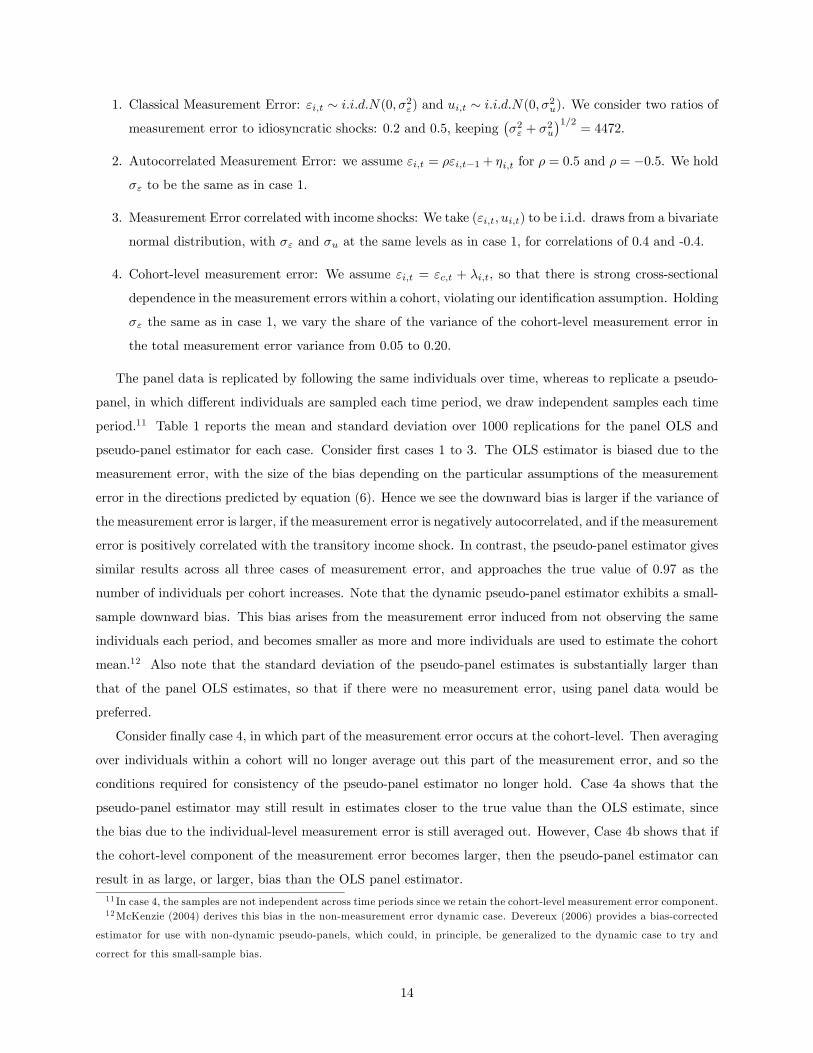
1. Classical Measurement Error: εi,t ∼ i.i.d.N(0, σ2ε) and ui,t ∼ i.i.d.N(0, σ2u). We consider two ratios of

measurement error to idiosyncratic shocks: 0.2 and 0.5, keeping¡σ2ε + σ2u

¢1/2= 4472.

2. Autocorrelated Measurement Error: we assume εi,t = ρεi,t−1+ ηi,t for ρ = 0.5 and ρ = −0.5. We holdσε to be the same as in case 1.

3. Measurement Error correlated with income shocks: We take (εi,t, ui,t) to be i.i.d. draws from a bivariate

normal distribution, with σε and σu at the same levels as in case 1, for correlations of 0.4 and -0.4.

4. Cohort-level measurement error: We assume εi,t = εc,t + λi,t, so that there is strong cross-sectional

dependence in the measurement errors within a cohort, violating our identification assumption. Holding

σε the same as in case 1, we vary the share of the variance of the cohort-level measurement error in

the total measurement error variance from 0.05 to 0.20.

The panel data is replicated by following the same individuals over time, whereas to replicate a pseudo-

panel, in which different individuals are sampled each time period, we draw independent samples each time

period.11 Table 1 reports the mean and standard deviation over 1000 replications for the panel OLS and

pseudo-panel estimator for each case. Consider first cases 1 to 3. The OLS estimator is biased due to the

measurement error, with the size of the bias depending on the particular assumptions of the measurement

error in the directions predicted by equation (6). Hence we see the downward bias is larger if the variance of

the measurement error is larger, if the measurement error is negatively autocorrelated, and if the measurement

error is positively correlated with the transitory income shock. In contrast, the pseudo-panel estimator gives

similar results across all three cases of measurement error, and approaches the true value of 0.97 as the

number of individuals per cohort increases. Note that the dynamic pseudo-panel estimator exhibits a small-

sample downward bias. This bias arises from the measurement error induced from not observing the same

individuals each period, and becomes smaller as more and more individuals are used to estimate the cohort

mean.12 Also note that the standard deviation of the pseudo-panel estimates is substantially larger than

that of the panel OLS estimates, so that if there were no measurement error, using panel data would be

preferred.

Consider finally case 4, in which part of the measurement error occurs at the cohort-level. Then averaging

over individuals within a cohort will no longer average out this part of the measurement error, and so the

conditions required for consistency of the pseudo-panel estimator no longer hold. Case 4a shows that the

pseudo-panel estimator may still result in estimates closer to the true value than the OLS estimate, since

the bias due to the individual-level measurement error is still averaged out. However, Case 4b shows that if

the cohort-level component of the measurement error becomes larger, then the pseudo-panel estimator can

result in as large, or larger, bias than the OLS panel estimator.11 In case 4, the samples are not independent across time periods since we retain the cohort-level measurement error component.12McKenzie (2004) derives this bias in the non-measurement error dynamic case. Devereux (2006) provides a bias-corrected

estimator for use with non-dynamic pseudo-panels, which could, in principle, be generalized to the dynamic case to try and

correct for this small-sample bias.

14

Overall, these Monte-Carlo results give us reason to be cautiously optimistic about using the pseudo-panel

estimator to estimate mobility. The small-sample bias will tend to result in an overstatement of mobility, as

will any classical cohort-level measurement error. Thus we can be reasonably confident that if we find low

levels of mobility using pseudo-panel methods, that mobility is indeed low.

5 Data

To investigate earnings mobility in Mexico we use the Encuesta Nacional de Empleo Urbano(ENEU), Mex-

ico’s national urban employment survey, conducted by the Instituto Nacional de Estadística, Geografía e

Informática (INEGI). The sampling unit is a dwelling or housing structure, and demographic information

is collected on the household or households occupying each dwelling. An employment questionnaire is then

administered for each individual aged 12 and above in the household, providing detailed information on

occupation, labor hours, labor earnings, and employment conditions. The survey is designed as a rotating

panel, with households interviewed for five consecutive quarters before exiting the survey. In each new round

the household questionnaire records absent members, adds any new members who have joined the house-

hold, and records any changes in schooling that have taken place. If none of the original group of household

members is found to be living in the dwelling unit in the follow-up survey, the household is recorded as a

new household (INEGI, 1998). As in many labor force surveys in developing countries, the interviewers do

not track households which move, so any household which moves attrits from the panel.

We use data from the first quarter of 1987 through to the second quarter of 200113, providing 58 quarters

of data. Over this period the ENEU expanded coverage from 16 cities in 1987 to 34 cities by the end of 1992

and 44 cities by the second quarter of 2001. We include all 39 cities present by the end of 1994, although

our results are robust to restricting the sample to just the 16 cities present in all years.

The ENEU only collects data on labor earnings for each household member in their principal occupation.

We add this over household members and deflate by the Consumer Price Index for the relevant quarter from

the Bank of Mexico to obtain real household labor earnings. To focus only on households for whom labor

earnings are likely to be a main source of income, we restrict our sample to households with heads aged 25

to 49 years old in the first wave of their respective panels. On average two percent of the observations have

household labor income of zero. Using data from the ENIGH income and expenditure survey, which does

include non-labor sources of income, we calculate that labor income represents 95 percent of total monetary

income for urban households with heads in the 25-49 year old age range. In Section 6.2 we examine how

mobility in labor earnings compares to estimated mobility in full income and in expenditure.

For our panel data analysis we then have 54 five-quarter panels, beginning with the panel of 3930 house-

holds which were sampled from the first quarter of 1987 through to the first quarter of 1988, and ending

13Since the second quarter of 2001, the ENEU was replaced by the ENE, which has now become the ENET - a national

quarterly employment survey.

15

with the panel of 11,158 households that were sampled from the second quarter of 2000 through to the

second quarter of 2001. We use unbalanced panels. Attrition is comparable to dwelling-based labor force

surveys in other developing countries. Ten percent of households are observed for only one quarter, while

approximately 65 percent of households can be followed for all five quarters.

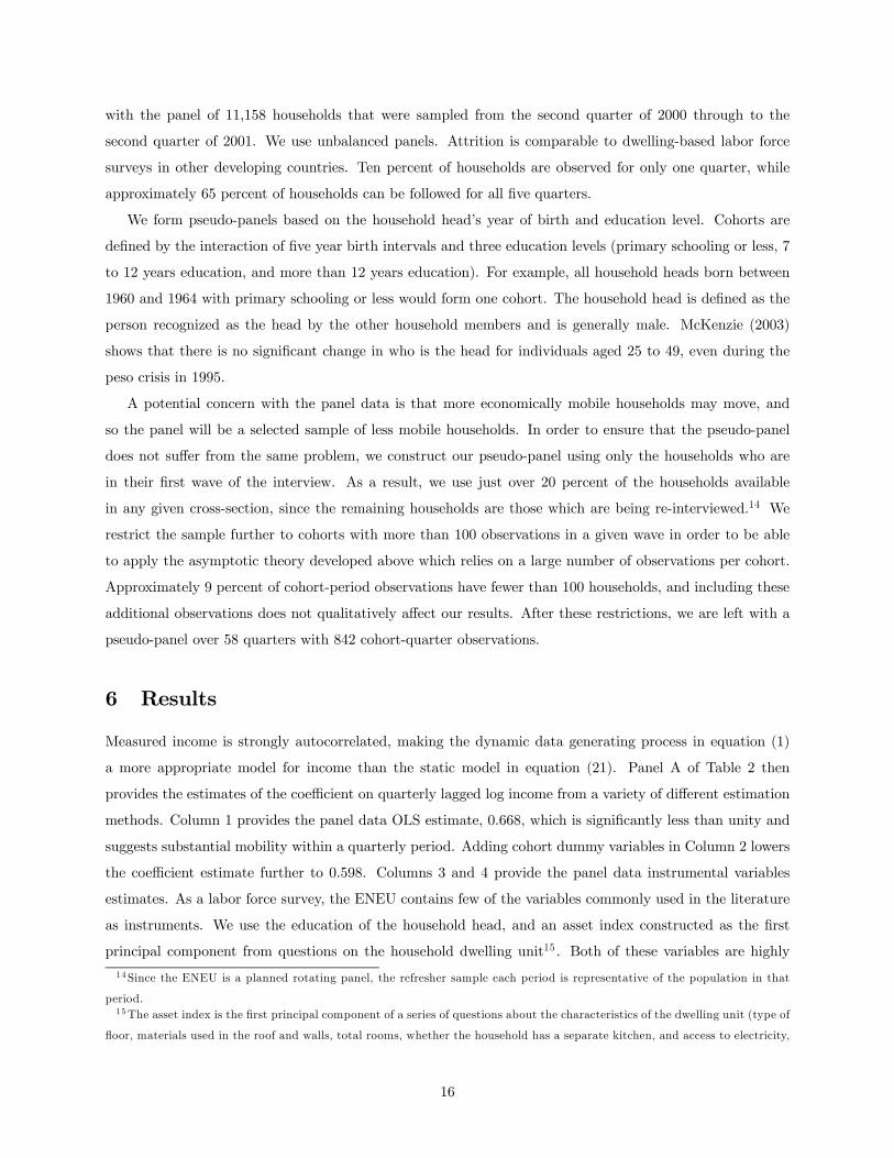
We form pseudo-panels based on the household head’s year of birth and education level. Cohorts are

defined by the interaction of five year birth intervals and three education levels (primary schooling or less, 7

to 12 years education, and more than 12 years education). For example, all household heads born between

1960 and 1964 with primary schooling or less would form one cohort. The household head is defined as the

person recognized as the head by the other household members and is generally male. McKenzie (2003)

shows that there is no significant change in who is the head for individuals aged 25 to 49, even during the

peso crisis in 1995.

A potential concern with the panel data is that more economically mobile households may move, and

so the panel will be a selected sample of less mobile households. In order to ensure that the pseudo-panel

does not suffer from the same problem, we construct our pseudo-panel using only the households who are

in their first wave of the interview. As a result, we use just over 20 percent of the households available

in any given cross-section, since the remaining households are those which are being re-interviewed.14 We

restrict the sample further to cohorts with more than 100 observations in a given wave in order to be able

to apply the asymptotic theory developed above which relies on a large number of observations per cohort.

Approximately 9 percent of cohort-period observations have fewer than 100 households, and including these

additional observations does not qualitatively affect our results. After these restrictions, we are left with a

pseudo-panel over 58 quarters with 842 cohort-quarter observations.

6 Results

Measured income is strongly autocorrelated, making the dynamic data generating process in equation (1)

a more appropriate model for income than the static model in equation (21). Panel A of Table 2 then

provides the estimates of the coefficient on quarterly lagged log income from a variety of different estimation

methods. Column 1 provides the panel data OLS estimate, 0.668, which is significantly less than unity and

suggests substantial mobility within a quarterly period. Adding cohort dummy variables in Column 2 lowers

the coefficient estimate further to 0.598. Columns 3 and 4 provide the panel data instrumental variables

estimates. As a labor force survey, the ENEU contains few of the variables commonly used in the literature

as instruments. We use the education of the household head, and an asset index constructed as the first

principal component from questions on the household dwelling unit15 . Both of these variables are highly

14Since the ENEU is a planned rotating panel, the refresher sample each period is representative of the population in that

period.15The asset index is the first principal component of a series of questions about the characteristics of the dwelling unit (type of

floor, materials used in the roof and walls, total rooms, whether the household has a separate kitchen, and access to electricity,

16

autocorrelated over time, and in accordance the result in equation (14), we obtain an estimate of β very close

to unity, 0.99. In contrast, when we employ the second lag of log income as an instrument and employ the

Arellano (1989) estimation method, the estimate of β is -0.062, which would indicate full origin independence

and in fact some slight reversal in income. This accords with our theoretical result that this estimate will

be biased towards zero.

Columns 5 and 6 provide our pseudo-panel estimates of β. When we do not allow for individual effects

through cohort-specific intercepts, the estimate of β is 0.988, while after allowing for individual effects we

obtain an estimate of β of 0.832. Comparing these results with those in Columns 1 through 4, we see that the

OLS estimates suggest much larger mobility than the pseudo-panel estimate, as does the Arellano estimate.

The IV estimate using instruments which are strongly autocorrelated happens to give results similar to the

pseudo-panel estimate for absolute mobility. This is a consequence of mobility being low over this quarterly

period: as equation (14) showed, we would expect to get a coefficient of 0.99 from the IV estimation here

regardless of the level of mobility in income, since education and the asset index do not vary much from one

period to the next.

Approximately two percent of our households have zero labor income in a given period, and are omitted

when calculating log income. In Panel B of Table 2 we therefore repeat the analysis using the level of

income, which allows us to include these zeros. The results are qualitatively very similar to those in Panel

A, suggesting that the exclusion of these few zero observations does not make a substantive difference.

The use of pseudo-panel analysis allows us to examine mobility over longer time periods than would be

possible with the five quarter genuine panels available in Mexico. Table 2 provides estimates of the mobility

coefficient over one quarter, one year, two year, and five year time periods. Since not all cohorts are aged

between 25 and 49 in every quarter, less cohort-period observations are available for longer intervals. Table

3 presents results from the balanced pseudo-panel, where the same cohort-quarter observations are used

for estimation over different time lags.16 Columns 1 through 4 provide the estimates of absolute mobility,

while Columns 5 through 8 include cohort fixed effects and therefore give measures of conditional mobility.

Absolute mobility increases slightly as one increases the time frame, but the estimate of β is still 0.933 over

two year intervals and 0.950 over five year intervals.17 Thus while poorer households experience slightly

faster income growth than richer households, a household which has 10 percent higher income than another

household today is estimated to still have 9.5 percent higher income five years later.

In contrast, Table 3 shows a high degree of conditional mobility. A ten percent difference in income

between two households with the same fixed effect is reduced to a 8.3 percent difference after one quarter,

a 5.5 percent difference after one year, and only a 0.5 percent difference after two years. By five years, the

sewerage, water and telephone). These questions have only been asked since the third quarter of 1994, and are only asked once

a year, so by assumption are perfectly autocorrelated within the year.16The point estimates for the unbalanced pseudo-panel are very similar to those for the balanced pseudo-panel and are

available upon request.17The five-year coefficient is not statistically significant from the two-year coefficient.

17

households have reversed rankings.

6.1 Mobility and Attrition

Measurement error will result in both OLS and IV methods giving inconsistent measures of mobility. How-

ever, a second source of potential bias in mobility estimates based on genuine panel data is that of non-random

attrition. This is particularly likely to be a concern in many developing country contexts in which panel

surveys track dwelling units, rather than households, over time. Thomas, Frankenberg and Smith (2001)

note that this is the standard protocol for follow-up surveys conducted as part of the World Bank’s Living

Standards Measurement Study, with second round follow-up rates of 87 percent in Cote d’Ivoire, 55 percent

in Peru, and 50 percent in Ghana. In the Mexican urban labor force survey used in this paper, 65 percent of

households are followed for all five quarters. Failure to follow households which move is likely to understate

mobility in both the OLS and IV estimates, since it appears likely that households which move dwellings

are likely to have experienced greater income changes than households which stay put. Although correction

for attrition is possible under certain structural assumptions, most studies of mobility do not attempt to

address this issue.18

We therefore now investigate how much of the difference between our pseudo-panel estimates and panel

data estimates is due to non-random attrition rather than measurement error. We begin by examining

the determinants of who attrits. Table 4 presents marginal effects from probit estimation of two types of

attrition. Column 1 considers households which attrit after only one round of interviews. These household

heads are younger, less likely to be married, have smaller household sizes and larger incomes than household

heads who remain for two or more waves of the survey. However, while these differences are significant given

the large number of observations, the magnitude of the effects is rather small. In Columns 2 through 5,

we look at households which appear in the first two quarters of the survey and examine the determinants

of attriting before their full five quarters are completed. This allows us to examine whether attrition is

related to the change in income experienced by the household between the first two waves. We find that

both the change in income or log income, and the absolute value of this change, are positively associated

with subsequent attrition from the panel. However, a one standard deviation change in either the change in

income or absolute value of the change in income is associated with less than a 0.01 increase in the probability

of attrition.

These results suggest that while attrition is more common amongst households which experience greater

income mobility, the magnitude of the bias is likely to be rather small. However, a concern might be

that households which experience the largest absolute changes in income move houses and attrit out of the

survey before the next quarter’s survey can be completed. Since these income movements are by assumption

unobserved, we can not directly examine them. Instead, in Table 5 we examine how much our pseudo-panel

estimates of absolute and conditional mobility differ when we consider only households which don’t attrit. We

18Recent exceptions are Lokshin and Ravallion (2004) and Duval-Hernández (2006).

18

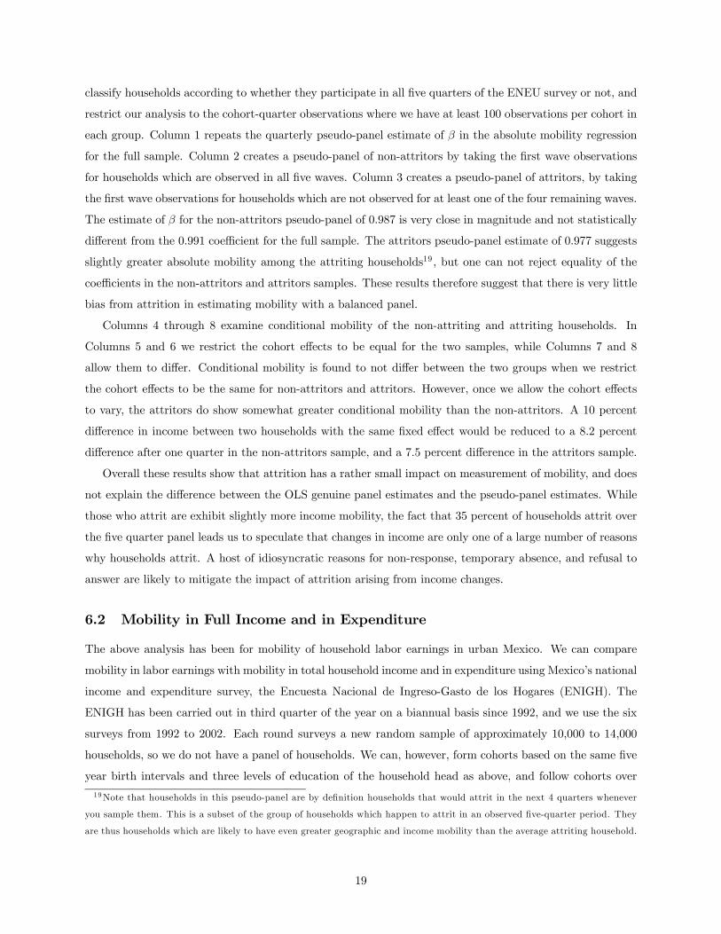
classify households according to whether they participate in all five quarters of the ENEU survey or not, and

restrict our analysis to the cohort-quarter observations where we have at least 100 observations per cohort in

each group. Column 1 repeats the quarterly pseudo-panel estimate of β in the absolute mobility regression

for the full sample. Column 2 creates a pseudo-panel of non-attritors by taking the first wave observations

for households which are observed in all five waves. Column 3 creates a pseudo-panel of attritors, by taking

the first wave observations for households which are not observed for at least one of the four remaining waves.

The estimate of β for the non-attritors pseudo-panel of 0.987 is very close in magnitude and not statistically

different from the 0.991 coefficient for the full sample. The attritors pseudo-panel estimate of 0.977 suggests

slightly greater absolute mobility among the attriting households19, but one can not reject equality of the

coefficients in the non-attritors and attritors samples. These results therefore suggest that there is very little

bias from attrition in estimating mobility with a balanced panel.

Columns 4 through 8 examine conditional mobility of the non-attriting and attriting households. In

Columns 5 and 6 we restrict the cohort effects to be equal for the two samples, while Columns 7 and 8

allow them to differ. Conditional mobility is found to not differ between the two groups when we restrict

the cohort effects to be the same for non-attritors and attritors. However, once we allow the cohort effects

to vary, the attritors do show somewhat greater conditional mobility than the non-attritors. A 10 percent

difference in income between two households with the same fixed effect would be reduced to a 8.2 percent

difference after one quarter in the non-attritors sample, and a 7.5 percent difference in the attritors sample.

Overall these results show that attrition has a rather small impact on measurement of mobility, and does

not explain the difference between the OLS genuine panel estimates and the pseudo-panel estimates. While

those who attrit are exhibit slightly more income mobility, the fact that 35 percent of households attrit over

the five quarter panel leads us to speculate that changes in income are only one of a large number of reasons

why households attrit. A host of idiosyncratic reasons for non-response, temporary absence, and refusal to

answer are likely to mitigate the impact of attrition arising from income changes.

6.2 Mobility in Full Income and in Expenditure

The above analysis has been for mobility of household labor earnings in urban Mexico. We can compare

mobility in labor earnings with mobility in total household income and in expenditure using Mexico’s national

income and expenditure survey, the Encuesta Nacional de Ingreso-Gasto de los Hogares (ENIGH). The

ENIGH has been carried out in third quarter of the year on a biannual basis since 1992, and we use the six

surveys from 1992 to 2002. Each round surveys a new random sample of approximately 10,000 to 14,000

households, so we do not have a panel of households. We can, however, form cohorts based on the same five

year birth intervals and three levels of education of the household head as above, and follow cohorts over

19Note that households in this pseudo-panel are by definition households that would attrit in the next 4 quarters whenever

you sample them. This is a subset of the group of households which happen to attrit in an observed five-quarter period. They

are thus households which are likely to have even greater geographic and income mobility than the average attriting household.

19

time. We consider two subsamples of the data. The first consists of urban households, defined as households

in areas of population 100,000 or more, which allows comparison with the ENEU survey. The second is rural

households in areas of population of 15,000 or fewer. Out of the 105 cohort-period observations, we have 82

observations in urban areas and only 53 observations in rural areas for which 100 or more households are

surveyed within the cohort.

We examine mobility in four different measures of household resources. The first is household income

from the primary occupation of each member, which is the measure used in the ENEU. The second, total

monetary income, includes all household cash income, including income earned from transfers, pensions,

rent, interest, and from non-primary jobs. The third measure, full income, adds non-monetary sources of

household income, which includes the value of all home-produced consumption and of any goods received

as transfers. The fourth measure is full expenditure, which includes all monetary expenditure and home-

produced consumption items. Over the six survey rounds household primary labor earnings has a correlation

of 0.91 with total monetary income, 0.83 with full income, and 0.58 with full expenditure.

Panel A of Table 6 presents the estimated slope coefficients from equation (19) for these four measures.

For urban households the four measures give very similar levels of absolute mobility. The estimates of β range

from 0.86 to 0.89. The rural estimates range from 0.65 (primary wage income) to 0.80 (full expenditure).

The point estimates would therefore suggest that there is more absolute mobility in rural areas than in urban

areas, and that rural wage income is more mobile than rural expenditure. However the limited number of

rural observations results in large standard errors and we can not reject equality of the rural and urban

coefficients. The coefficient on log primary wage income for urban households is 0.87 compared to 0.93 for

the equivalent measure in the ENEU data.20 This difference is not statistically significant.

Panel B of Table 6 adds cohort fixed effects and presents the estimated slope coefficients from equation

(20). The point estimates suggest very high rates of conditional mobility, with the slope coefficients close

to zero. The point estimates also show less conditional mobility in expenditure than in wage income. The

ENIGH data only includes 6 time periods, so with the inclusion of cohort fixed effects, identification of the

slope coefficient comes from within-cohort changes in income over this small number of periods. As a result,

the standard errors are large, giving wide confidence intervals for conditional mobility. Nevertheless, the

coefficient of 0.08 for urban primary wage income is very close to the 0.05 coefficient obtained using the

ENEU data.21

7 Interpretation

Our results show rather limited absolute mobility in income and expenditure in Mexico, but rapid conditional

mobility. In order to interpret this result further, recall the data generating equation for household income

20Since the ENIGH is taken in the third quarter of the year, a more appropriate comparison might be to the results from the

ENEU, using only interviews from the third quarter. This coefficient is 0.929, compared to the 0.936 coefficient in Table 3.21Using only the third quarter interviews of the ENEU, the coefficient is 0.155, with a 95% confidence interval of [0.02, 0.29].

20

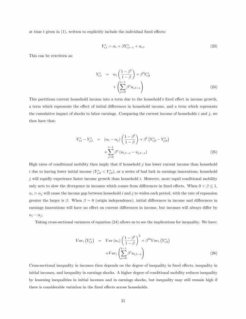
at time t given in (1), written to explicitly include the individual fixed effects:

Y ∗i,t = αi + βY ∗i,t−1 + ui,t (23)

This can be rewritten as:

Y ∗i,t = αi

µ1− βt

1− β

¶+ βtY ∗i,0

+

Ãt−1Xs=0

βsui,t−s

!(24)

This partitions current household income into a term due to the household’s fixed effect in income growth,

a term which represents the effect of initial differences in household income, and a term which represents

the cumulative impact of shocks to labor earnings. Comparing the current income of households i and j, we

then have that:

Y ∗i,t − Y ∗j,t = (αi − αj)

µ1− βt

1− β

¶+ βt

¡Y ∗i,0 − Y ∗j,0

¢+

t−1Xs=0

βs (ui,t−s − uj,t−s) (25)

High rates of conditional mobility then imply that if household j has lower current income than household

i due to having lower initial income (Y ∗j,0 < Y ∗i,0), or a series of bad luck in earnings innovations, household

j will rapidly experience faster income growth than household i. However, more rapid conditional mobility

only acts to slow the divergence in incomes which comes from differences in fixed effects. When 0 < β ≤ 1,αi > αj will cause the income gap between household i and j to widen each period, with the rate of expansion

greater the larger is β. When β = 0 (origin independence), initial differences in income and differences in

earnings innovations will have no effect on current differences in income, but incomes will always differ by

αi − αj .

Taking cross-sectional variances of equation (24) allows us to see the implications for inequality. We have:

V ari¡Y ∗i,t¢= V ar (αi)

µ1− βt

1− β

¶2+ β2tV ari

¡Y ∗i,0

¢+V ari

Ãt−1Xs=0

βsui,t−s

!(26)

Cross-sectional inequality in incomes then depends on the degree of inequality in fixed effects, inequality in

initial incomes, and inequality in earnings shocks. A higher degree of conditional mobility reduces inequality

by lessening inequalities in initial incomes and in earnings shocks, but inequality may still remain high if

there is considerable variation in the fixed effects across households.

21

In terms of the concepts used to motivate the study of mobility, one interpretation is to consider the

αi’s as measuring a combination of innate differences in earnings ability and of differences in ‘opportunity’.

Inequality in the fixed effects therefore would reflect differences in the education and health care of individ-

uals, as well as factors such as discrimination which prevents certain individuals from being able to work

in particular occupations. Under this view, β can then be seen as measuring the degree of flexibility and

freedom in the labor market. Given predetermined individual attributes, β measures how rapidly individuals

who are earning too little or too much relative to their individual abilities and opportunities regress to their

mean level of earnings.

Our finding of slow absolute mobility but rapid conditional mobility has several implications for further

study of Mexican income differences. Our finding of rapid conditional mobility suggests that households

are able to recover quickly from bad luck and shocks to labor earnings, and therefore that the high level of

inequality in Mexican income is not due to income shocks having long-term effects. However, the high rate

of conditional mobility coupled with the fact that absolute mobility remains low means that household fixed

effects are important and that income differences among households will persist over many years. These fixed

effects represent everything specific to a household that has a persistent effect on their income. This includes

the education, language, gender, and birth cohort of the household head; household demographic factors; the

institutional environment facing a particular household; and other factors that determine labor income such

as innate ability, ability to work with others, and entrepreneurial prowess. The challenge for future work is

to determine the types of policy interventions which can reduce differences in these fixed effects. Examples

may include interventions in health and education and improvements in labor market institutions.

8 Conclusions

We have shown that dynamic pseudo-panel estimation can be used to consistently estimate the degree of

earnings mobility, allowing mobility estimation even when genuine panels are not available. When earnings

dynamics are generated by a dynamic linear model, we estimate full mobility, whereas if earnings have a

static data generating process, our estimator recovers longer-term mobility, but like all estimators, can not

distinguish mobility due to temporary idiosyncratic income level shocks from mobility due to measurement

error. However, given a dynamic data generating process, our method is consistent, even in the presence

of non-classical measurement errors. Although pseudo-panel estimation also greatly reduces the potential

bias from attrition of the most mobile, in our sample we find only relatively small differences in mobility

estimation arising from attrition.

In related work, Antman and McKenzie (2006) find that there is no evidence for a poverty trap in income

in Mexico. While this is reassuring, the results here indicate that overall mobility in earnings, income,

and expenditure, is very low in Mexico. However, households are quite mobile around their individual

effects. This suggests a role for policy interventions which aim to lower inequality amongst households in the

22

attributes they bring to the labor market, such as the education and health interventions occurring under

the Oportunidades program.

Appendix 1:

Consider:

bβIV = β +

1N

NPi=1(ui,t + εi,t − βεi,t−1) zi,t−1

1N

NPi=1

Yi,t−1zi,t−1

(27)

Let us consider each of the various components of the numerator of the fraction in (27). A standard law of

large numbers gives that:

1

N

NXi=1

εi,tzi,t−1p→ E (εi,tzi,t−1) (28)

1

N

NXi=1

εi,t−1zi,t−1p→ E (εi,t−1zi,t−1) (29)

Consider next the term (1/N)PN

i=1 ui,tzi,t−1. To examine this term, first substitute equation (11) into (9)

to get:

Yi,t = φ+ γμ+ γρZi,t−1 + γωi,t + vi,t + εi,t (30)

Next substitute (9) into (4) to get:

Yi,t = α+ βφ+ βγZi,t−1 + βvi,t−1 + ui,t + εi,t (31)

Equating equations (31) and (30) then gives:

ui,t = (φ+ γμ− α− βφ) + γ (ρ− β)Zi,t−1

+γωi,t + vi,t − βvi,t−1 (32)

From (32) we then have:

1

N

NXi=1

ui,tzi,t−1

p→ γ (ρ− β)V ar (Zi,t−1) + λ (33)

where

23

λ = γE (ωi,tZi,t−1) +E (vi,tZi,t−1)− βE (vi,t−1Zi,t−1) (34)

From (9) we also have that the denominator:

1

N

NXi=1

Yi,t−1zi,t−1p→ γV ar (Zi,t−1) +E (Zi,t−1εi,t−1) +E (Zi,t−1vi,t−1) (35)

Substituting (28), (29), (33) and (35) into (27) gives equation (12).

24

References:Antman, Francisca and David J. McKenzie (2006) “Poverty Traps and Nonlinear Income Dynamics with

Measurement Error and Individual Heterogeneity”, forthcoming, Journal of Development Studies.Arellano, Manuel (1989) “A Note on the Anderson-Hsiao Estimator for Panel Data”, Economics Letters

31: 337-41.Arellano, M. and S. Bond (1991) “Some tests of specification for panel data: Monte Carlo evidence and

an application to employment equations”, Review of Economic Studies 58: 277-97.Atkinson, A.B., F. Bourguignon and C. Morrisson (1992) Empirical Studies of Earnings Mobility, Fun-

damentals of Pure and Applied Economics 52, Harwood Academic Publishers: Philadelphia.Barro, Robert J. and Xavier Sala-i-Martin (1999) Economic Growth. The MIT Press: Cambridge, MA.Bound, John, Charles Brown and Nancy Mathiowetz (2001) “Measurement Error in Survey Data”, pp.

3705-3843 in J.J. Heckman and E. Leamer (eds.) Handbook of Econometrics Volume 5. Elsevier Science:Amsterdam.Bound, John and Alan Krueger (1991) “The Extent of Measurement Error in Longitudinal Earnings

Data: Do Two Wrongs Make a Right?”, Journal of Labor Economics 9:1-24.Carter, Michael and Christopher Barrett (2006) “The Economics of Poverty Traps and Persistent Poverty:

An Asset-Based Approach”, Journal of Development Studies 42(2): 178-99.Chang, Yoosoon (2002) “Nonlinear IV Unit Root Tests in Panels with Cross-Sectional Dependency”,

Journal of Econometrics 110(2): 261-92.Collado, M. Dolores (1997) “Estimating dynamic models from time series of independent cross-sections”,

Journal of Econometrics 82(1): 37-62.Deaton, Angus (1985) “Panel data from time series of cross-sections”, Journal of Econometrics 30: 109-

126.Devereux, Paul (2006) “Improved Errors-in-Variables Estimators for Grouped Data”, forthcoming, Jour-

nal of Business and Economic Statistics.Dragoset, Lisa and Gary Fields (2006) “U.S. Earnings Mobility: Comparing Survey-Based and Administrative-

Based Estimates”, Mimeo. Cornell University.Duval-Hernández, Robert (2006) “Dynamics of Labor Market Earnings in Urban Mexico 1987-2002”,

Mimeo. Center for U.S.-Mexican Studies, UCSD.Fields, Gary, Paul L. Cichello, Samuel Freije, Marta Menéndez and David Newhouse (2003) “For Richer

or for Poorer? Evidence from Indonesia, South Africa, Spain and Venezuela”, Journal of Economic Inequality1: 67-99.Fields, Gary, Robert Duval-Hernández, Samuel Freije Rodríguez and María Laura Sánchez Puerta (2006)

“Earnings Mobility in Argentina, Mexico, and Venezuela: Testing the Divergence of Earnings and theSymmetry of Mobility Hypotheses”, Mimeo. Cornell University.Fields, Gary and Efe Ok (1999) “The Measurement of Income Mobility: An Introduction to the Liter-

ature”, pp. 557-598 in J. Silber (eds.) Handbook of Income Inequality Measurement, Springer-Verlag: NewYork.Glewwe, Paul and Phong Nguyen (2002) “Economic Mobility in Vietnam in the 1990s”, World Bank

Policy Research Working Paper No. 2838.Gottschalk, Peter (1997) “Inequality, Income Growth, and Mobility: The Basic Facts”, Journal of Eco-

nomic Perspectives 11(2): 21-40.Gottschalk, Peter and Enrico Spolaore (2002) “On the evaluation of economic mobility”, Review of

Economic Studies 69: 191-208.Instituto Nacional de Estadística, Geografía e Informática (INEGI) (1998) Documento Metodológico de

la Encuesta Nacional de Empleo Urbano (Methodological Document of the National Urban EmploymentSurvey), INEGI: Aguascalientes, Mexico.Islam, Nazrul (1995) “Growth Empirics: A Panel Data Approach”, Quarterly Journal of Economics

110(4): 1127-70.Jarvis, Sarah and Stephen P. Jenkins (1998) “How much income mobility is there in Britain”, The

Economic Journal, 108: 428-443.Lokshin, Michael and Martin Ravallion (2004). “Household Income Dynamics in Two Transition Economies”,

Studies in Nonlinear Dynamics and Econometrics 8(3), Article 4.http://www.bepress.com/snde/vol8/iss3/art4Luttmer, Erzo F.P. (2002) “Measuring Economic Mobility and Inequality: Disentangling Real Events

from Noisy Data”, Mimeo. Harris School of Public Policy Studies, University of Chicago.McCulloch, Neil and Bob Baulch (2000) “Simulating the Impact of Policy Upon Chronic and Transitory

Poverty in Rural Pakistan”, Journal of Development Studies 36(6): 100-130.McKenzie, David J. (2001a) “Estimation of AR(1) models with unequally-spaced pseudo-panels”, Econo-

metrics Journal, 4: 89- 108

25

McKenzie, David J. (2001b) “Consumption Growth in a Booming Economy: Taiwan 1976-96”, YaleUniversity Economic Growth Center Discussion Paper No. 823.McKenzie, David J. (2003) “How do Households Cope with Aggregate Shocks? Evidence from the

Mexican Peso Crisis”, World Development 31(7): 1179-99.McKenzie, David J. (2004) “Asymptotic theory for heterogeneous dynamic pseudo-panels”, Journal of

Econometrics 120(2): 235-262.Moffitt, Robert (1993) “Identification and estimation of dynamic models with a time series of repeated

cross-sections”, Journal of Econometrics 59(1): 99-124.Piketty, Thomas (2000) “Theories of Persistent Inequality and Intergenerational Mobility”, Chapter 8,

pp. 429- 476 in A.B. Atkinson and F. Bourguignon (eds.) Handbook of Income Distribution Volume 1,North-Holland: AmsterdamStrauss, John, Kathleen Beegle, Agus Dwiyanto, Yulia Herawati, Daan Pattinasarany, Elan Satriawan,

Bondan Sikoki, Sukamdi and Firman Witoelar (2004) Indonesian Living Standards before and after thefinancial crisis: Evidence from the Indonesia Family Life Survey, RAND Corporation: Santa Monica.Thomas, Duncan, Elizabeth Frankenberg and James P. Smith (2001) “Lost but not Forgotten: Attrition

and Follow-up in the Indonesia Family Life Survey”, Journal of Human Resources 36(3): 556-592.Verbeek, Marno and Francis Vella (2005) “Estimating dynamic models from repeated cross-sections”,

Journal of Econometrics 127(1): 83-102.

26

TABLE 1: MONTE-CARLO COMPARISON OF OLS AND PSEUDO-PANEL RESULTSFor β = 0.97, T=2 periods

βOLS βPSEUDO βOLS βPSEUDO

1. Classical Measurement Error n = 200, C = 18 0.873 0.956 0.729 0.953

(0.013) (0.082) (0.017) (0.072) n = 1000, C = 18 0.872 0.969 0.729 0.965

(0.006) (0.030) (0.012) (0.028)2. Autocorrelated Measurement Errora. Rho = +0.5 n = 200, C = 18 0.924 0.937 0.853 0.936

(0.012) (0.072) (0.012) (0.065) n = 1000, C = 18 0.923 0.965 0.853 0.962

(0.005) (0.031) (0.007) (0.029)b. Rho = -0.5 n = 200, C = 18 0.822 0.935 0.603 0.939

(0.082) (0.069) (0.020) (0.068) n = 1000, C = 18 0.823 0.963 0.602 0.964

(0.009) (0.033) (0.017) (0.030)3. Measurement error correlated with ui,t

a. Rho = +0.4 n = 200, C = 18 0.819 0.932 0.686 0.928

(0.014) (0.079) (0.017) (0.075) n = 1000, C = 18 0.819 0.965 0.686 0.963

(0.008) (0.035) (0.012) (0.034)b. Rho = -0.4 n = 200, C = 18 0.947 0.943 0.788 0.942

(0.012) (0.068) (0.016) (0.060) n = 1000, C = 18 0.947 0.967 0.787 0.963

(0.005) (0.030) (0.012) (0.028)4. Cohort-level measurement errora. cohort m.e. is 5% of individual n = 200, C = 18 0.872 0.901 0.728 0.860

(0.016) (0.099) (0.020) (0.120) n = 1000, C = 18 0.874 0.927 0.728 0.877

(0.010) (0.073) (0.016) (0.110)b. cohort m.e. is 20% of individual n = 200, C = 18 0.873 0.814 0.731 0.692

(0.022) (0.142) (0.032) (0.188) n = 1000, C = 18 0.874 0.835 0.723 0.698

(0.017) (0.127) (0.029) (0.175)Note: standard deviations shown in parentheses from 1000 replications.

More Measurement ErrorLess Measurement ErrorVar(e)/[Var(e)+Var(u)] =0.2 Var(e)/[Var(e)+Var(u)] =0.5

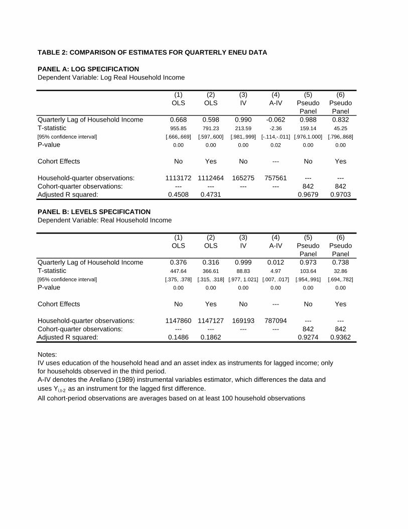
TABLE 2: COMPARISON OF ESTIMATES FOR QUARTERLY ENEU DATA

PANEL A: LOG SPECIFICATIONDependent Variable: Log Real Household Income

(1) (2) (3) (4) (5) (6)OLS OLS IV A-IV Pseudo Pseudo

Panel PanelQuarterly Lag of Household Income 0.668 0.598 0.990 -0.062 0.988 0.832T-statistic 955.85 791.23 213.59 -2.36 159.14 45.25[95% confidence interval] [.666,.669] [.597,.600] [.981,.999] [-.114,-.011] [.976,1.000] [.796,.868]P-value 0.00 0.00 0.00 0.02 0.00 0.00

Cohort Effects No Yes No --- No Yes

Household-quarter observations: 1113172 1112464 165275 757561 --- ---Cohort-quarter observations: --- --- --- --- 842 842Adjusted R squared: 0.4508 0.4731 0.9679 0.9703

PANEL B: LEVELS SPECIFICATIONDependent Variable: Real Household Income

(1) (2) (3) (4) (5) (6)OLS OLS IV A-IV Pseudo Pseudo

Panel PanelQuarterly Lag of Household Income 0.376 0.316 0.999 0.012 0.973 0.738T-statistic 447.64 366.61 88.83 4.97 103.64 32.86[95% confidence interval] [.375, .378] [.315, .318] [.977, 1.021] [.007, .017] [.954,.991] [.694,.782]P-value 0.00 0.00 0.00 0.00 0.00 0.00

Cohort Effects No Yes No --- No Yes

Household-quarter observations: 1147860 1147127 169193 787094 --- ---Cohort-quarter observations: --- --- --- --- 842 842Adjusted R squared: 0.1486 0.1862 0.9274 0.9362

Notes:IV uses education of the household head and an asset index as instruments for lagged income; onlyfor households observed in the third period.A-IV denotes the Arellano (1989) instrumental variables estimator, which differences the data anduses Yi,t-2 as an instrument for the lagged first difference. All cohort-period observations are averages based on at least 100 household observations

TABLE 3: MOBILITY OVER DIFFERENT TIME INTERVALSPseudo-Panel Estimates from the ENEU

Dependent Variable: Log Real Household Income

(1) (2) (3) (4) (5) (6) (7) (8)Quarterly Yearly 2-Year 5-Year Quarterly Yearly 2-Year 5-Year

Lagged Log Household Income 0.988 0.963 0.936 0.950 0.855 0.536 0.051 -0.498T-statistic 139.59 76.8 50.75 31.26 34.57 13.44 1.12 -13.63[95% confidence interval] [.974,1.002] [.938,.987] [.899,.972] [.890,1.010] [.807,.904] [.458,.614] [ -.038,.140] [ -.570,-.427]

Cohort Effects No No No No Yes Yes Yes YesCohort-quarter observations: 477 477 477 477 477 477 477 477Adjusted R squared: 0.9762 0.9253 0.844 0.6722 0.977 0.9406 0.9174 0.9411

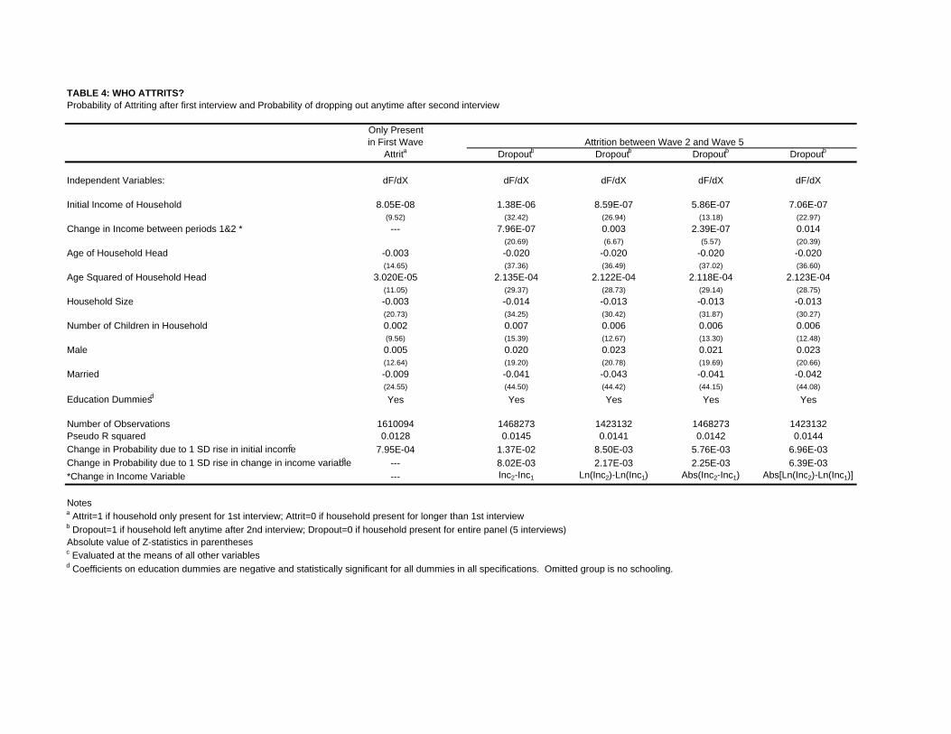
TABLE 4: WHO ATTRITS?Probability of Attriting after first interview and Probability of dropping out anytime after second interview

Only Presentin First Wave

Attrita Dropoutb Dropoutb Dropoutb Dropoutb

Independent Variables: dF/dX dF/dX dF/dX dF/dX dF/dX

Initial Income of Household 8.05E-08 1.38E-06 8.59E-07 5.86E-07 7.06E-07(9.52) (32.42) (26.94) (13.18) (22.97)

Change in Income between periods 1&2 * --- 7.96E-07 0.003 2.39E-07 0.014(20.69) (6.67) (5.57) (20.39)

Age of Household Head -0.003 -0.020 -0.020 -0.020 -0.020(14.65) (37.36) (36.49) (37.02) (36.60)

Age Squared of Household Head 3.020E-05 2.135E-04 2.122E-04 2.118E-04 2.123E-04(11.05) (29.37) (28.73) (29.14) (28.75)

Household Size -0.003 -0.014 -0.013 -0.013 -0.013(20.73) (34.25) (30.42) (31.87) (30.27)

Number of Children in Household 0.002 0.007 0.006 0.006 0.006(9.56) (15.39) (12.67) (13.30) (12.48)

Male 0.005 0.020 0.023 0.021 0.023(12.64) (19.20) (20.78) (19.69) (20.66)

Married -0.009 -0.041 -0.043 -0.041 -0.042(24.55) (44.50) (44.42) (44.15) (44.08)

Education Dummiesd Yes Yes Yes Yes Yes

Number of Observations 1610094 1468273 1423132 1468273 1423132Pseudo R squared 0.0128 0.0145 0.0141 0.0142 0.0144Change in Probability due to 1 SD rise in initial incomec 7.95E-04 1.37E-02 8.50E-03 5.76E-03 6.96E-03Change in Probability due to 1 SD rise in change in income variablec --- 8.02E-03 2.17E-03 2.25E-03 6.39E-03*Change in Income Variable --- Inc2-Inc1 Ln(Inc2)-Ln(Inc1) Abs(Inc2-Inc1) Abs[Ln(Inc2)-Ln(Inc1)]

Notesa Attrit=1 if household only present for 1st interview; Attrit=0 if household present for longer than 1st interviewb Dropout=1 if household left anytime after 2nd interview; Dropout=0 if household present for entire panel (5 interviews)Absolute value of Z-statistics in parenthesesc Evaluated at the means of all other variablesd Coefficients on education dummies are negative and statistically significant for all dummies in all specifications. Omitted group is no schooling.

Attrition between Wave 2 and Wave 5

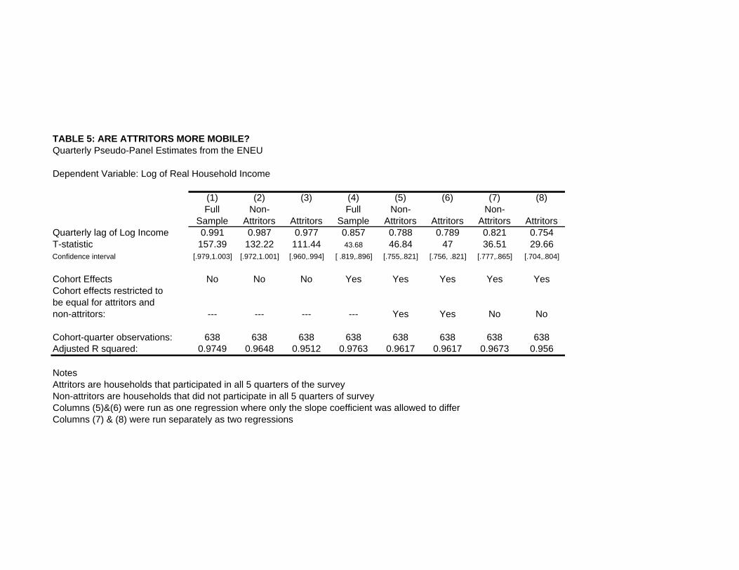
TABLE 5: ARE ATTRITORS MORE MOBILE?Quarterly Pseudo-Panel Estimates from the ENEU

Dependent Variable: Log of Real Household Income

(1) (2) (3) (4) (5) (6) (7) (8)Full Non- Full Non- Non-

Sample Attritors Attritors Sample Attritors Attritors Attritors AttritorsQuarterly lag of Log Income 0.991 0.987 0.977 0.857 0.788 0.789 0.821 0.754T-statistic 157.39 132.22 111.44 43.68 46.84 47 36.51 29.66Confidence interval [.979,1.003] [.972,1.001] [.960,.994] [ .819,.896] [.755,.821] [.756, .821] [.777,.865] [.704,.804]

Cohort Effects No No No Yes Yes Yes Yes YesCohort effects restricted to be equal for attritors and non-attritors: --- --- --- --- Yes Yes No No

Cohort-quarter observations: 638 638 638 638 638 638 638 638Adjusted R squared: 0.9749 0.9648 0.9512 0.9763 0.9617 0.9617 0.9673 0.956

NotesAttritors are households that participated in all 5 quarters of the surveyNon-attritors are households that did not participate in all 5 quarters of surveyColumns (5)&(6) were run as one regression where only the slope coefficient was allowed to differColumns (7) & (8) were run separately as two regressions

TABLE 6: MOBILITY IN INCOME AND EXPENDITURE Pseudo-panel estimates from the ENIGH Survey for two year lag

PANEL A: ABSOLUTE MOBILITY (NO COHORT FIXED EFFECTS)

Log Log Log LogPrimary Total Log Log Primary Total Log LogWage Monetary Full Full Wage Monetary Full Full

Income Income Income Expenditure Income Income Income ExpenditureTwo-year Lag 0.870 0.880 0.859 0.888 0.653 0.641 0.700 0.797(T-statistic) (14.69) (14.45) (13.20) (15.08) (5.07) (4.91) (5.52) (7.06)[confidence interval] [.75,.99] [.76,1.00] [.73,.99] [.77,1.01] [.39,.91] [.38,.91] [.44,.96] [.57,1.02]

Cohort-Period Observations: 61 61 61 61 40 40 40 40Adjusted R2 0.782 0.776 0.743 0.791 0.388 0.372 0.431 0.556

PANEL B: CONDITIONAL MOBILITY (COHORT FIXED EFFECTS)

Log Log Log LogPrimary Total Log Log Primary Total Log LogWage Monetary Full Full Wage Monetary Full Full

Income Income Income Expenditure Income Income Income ExpenditureTwo-year Lag 0.080 0.061 0.170 0.282 -0.078 -0.032 0.142 0.093(T-statistic) (0.52) (0.37) (0.98) (1.73) (0.44) (0.17) (0.74) (0.47)[confidence interval] [-.23, .39] [-.28,.40] [-.18,.52] [-.05,.61] [-.43,.28] [-.42,.36] [-.25,.53] [-.31,.50]

Cohort-Period Observations: 61 61 61 61 40 40 40 40Adjusted R2 0.838 0.827 0.780 0.824 0.611 0.540 0.530 0.659

Notes:Absolute value of pseudo-panel t-statistic in parentheses.Cohorts are defined by 5 year birth interval and three education groups.Source: own calculations from the 1992-2002 ENIGH surveys.

URBAN RURAL

URBAN RURAL