Early-Life Conditions, Parental Investments, and Child

Development: Evidence from a Violent Conflict

Valentina Duque∗

Columbia University

November 15, 2014

Abstract

A growing body of evidence finds that early-life circumstances are an important

determinant of an individual’s future outcomes. Here I investigate how shocks in

utero and in childhood affect human capital formation, and to what extent their

experience at certain developmental stages matters more than others. I focus on

violent conflicts that constitute multidimensional shocks to the well-being of many

households in developing countries. Using monthly and municipality-level variation

in the timing and severity of massacres in Colombia from 1999 to 2007, I show that

children exposed to sudden changes in violence in utero and in childhood achieve lower

height-for-age (0.09 SD), cognitive (PPVT falls by 0.17 SD and verbal ability, math

reasoning, and general knowledge fall by 0.15–0.28 SD), and socio-emotional outcomes

(adequate interaction falls by 0.04 SD). Furthermore, I explore changes in parental

investments as potential mechanisms, finding that changes in violence during a child’s

early-life is associated with lower quantity and quality of parenting. Results do not

seem to be driven by selective sorting, migration, fertility, or survival, and are robust

to controlling for mother fixed-effects. This is the first study to investigate the effects

of early-life violence on child cognitive and non-cognitive outcomes in a developing

country and among the first to investigate the role of parenting as a potential channel

of transmission.

Keywords: Human capital formation, Early-life shocks, Violence, Children, Development

JEL codes: J24, J13, D79, I20, O15

∗Email: vd2220@columbia.edu, PhD in Social Policy, Columbia University. I would like to thank my

advisors Doug Almond and Julien Teitler for guidance and support. I would also like to thank Janet

Currie, Ana Maria Ibanez, Fabio Sanchez, Adriana Camacho, Raquel Bernal, Camila Fernandez, Amy

Claessens, Bob George, Ivar Frones, Jane Waldfogel, Lena Edlund, Jennifer Dowd, Florencia Torche,

Orazio Attanasio, Costas Meghir, Maria Rosales, Mike Mueller, Natasha Pilkauskas, Elia De la Cruz, and

Pablo Ottonello for their very useful suggestions. I am indebted to the participants of APPAM 2014,

NEUDC 2014, the Child Indicators Workshop in Child Well-being 2014, CUNY Student Applied Micro

Seminar, PAA 2014, HiCN 2013, Olympia 2013 Workshop, Mellon Interdisciplinary Fellows Seminar,

Student Policy Seminar, Applied Micro Colloquium, and the Mailman School of Public Health (Columbia

University). Funding for this project was generously provided by the Hewlett/IIE Dissertation Fellowship

and the Mellon Interdisciplinary Fellow Program at Columbia University. All errors are my own.

1

Growing research points to the important role that early-life conditions play in shap-

ing adult outcomes (Barker, 1992; Cunha and Heckman, 2007; Almond and Currie, 2011).

Evidence from natural experiments shows that adverse conditions during the in-utero and

childhood periods (i.e., disease outbreaks, famines and malnutrition, weather shocks, ion-

izing radiation, earthquakes, air pollution) can have negative effects on health, education,

and labor market outcomes (e.g., Almond, 2006; Almond et al., 2010; Van den Berg et al.,

2006; Currie and Rossin-Slater, 2013; Almond, Edlund and Palme, 2009; Sanders, 2012).

In this study, I focus on perhaps one of the most pervasive shocks that affect individual’s

well-being: Exposure to violence (i.e., wars, armed conflicts, urban crime). The World

Bank (2013) estimates that more than 1.5 billion people in the developing world live

in chronically violent contexts. Violence creates poverty, accentuates inequality, destroys

infrastructure, displaces populations, disrupts schooling, and affects health. Moreover, I

focus on children, which is a particularly vulnerable subpopulation: Children in developing

countries are subject to more and more frequent adverse conditions, start disadvantaged,

and receive lower levels of investments compared with children from wealthier environ-

ments (Currie and Vogl, 2013).

While recent research has shown the large damage on education and health outcomes

from early life violence (Camacho, 2008; Akresh, Lucchetti and Thirumurthy, 2012; Mi-

noiu and Shemyakina, 2012; Brown, 2014; Valente, 2011; Leon, 2012), several key questions

remain unaddressed. First, how does violence affect other domains of human capital beside

education and health (i.e., cognitive and noncognitive skills)? Identifying such effects is

important both because measures of human capital (physical, cognitive, and non-cognitive

indicators) can explain a large percentage of the variation in later-life educational attain-

ment and wages (Currie and Thomas, 1999; McLeod and Kaiser, 2004; Heckman, Stixrud

and Urzua, 2006) and to understand mechanisms behind previous effects found for educa-

tional attainment and health. Second, to what extent do the effects of violence at different

developmental stages (i.e., in-utero vs. in childhood) differ? Do impacts on the particular

type of skill considered (e.g., health vs. cognitive outcomes) differ by the developmental

timing of the shock? Third, given the size and persistence of the effects of violence, it

is also natural to ask whether and how parental investments also may respond to these

shocks. Family investments are important determinants of human capital (Cunha and

Heckman, 2007; Aizer and Cunha, 2014) and parental responses can play a key role in

compensating or reinforcing the effects of a shock (Almond and Currie, 2011). At present,

well-identified empirical evidence on this question is scarce. Finally, and perhaps most

importantly from a policy perspective, is there potential for remediation: Can social pro-

grams that are available to the community help mitigate the negative effects of violence

on vulnerable children?

To explore these questions, I analize survey microdata on 21,000 children collected in

2007 to evaluate the largest social program in Colombia: a home-based childcare program

2

known as Hogares Comunitarios de Bienestar (HCB). HCB was implemented in the 1980s

and currently operates nationwide. The goal of the program is to promote low-income chil-

dren’s physical growth, health, and cognitive and socio-emotional development, as well as

to enhance women’s participation in the labor market. Poor families send their children

to a HCB center in the community where they receive childcare, nutritional support (50

to 70 percent of the recommended daily allowance), and psychosocial stimulation. HCB

serves approximately 800,000 low-income children between 0 and 7 years of age through-

out most of Colombia’s 1,100 municipalities (Bernal and Fernandez, 2013). The household

survey provides rich measures on child development, as well as detailed information on

parental investments and parenting behaviors. Most importantly, these data contain in-

formation on each child’s year and month of birth, as well as household migration history,

which allows me to identify with some precision a child’s violence exposure in utero and in

childhood. The data also include a small sample of siblings that I use to estimate models

that account for mother fixed-effects.

I measure violence shocks using the occurrence and severity of massacres at the

monthly and municipality levels during Colombia’s armed conflict. Massacres are de-

fined as the intentional killing of four or more people by another person or group. As

discussed in more detail in the background section, these shocks were a common practice

employed by violent groups during the most intense years of the conflict. From 1999–2007,

the period of interest in this paper, more than 1,000 massacres occurred across more than

half of all municipalities in the country, ranging from 4 to more than 25 victims killed in

each episode; as such, they represented significant shocks to a household’s well-being.

This paper exploits the large temporal and geographical variation in violence at the

municipality and month-year levels in Colombia from 1999 to 2007, to estimate the ef-

fects of violence on children and families. While the occurrence of massacres in a given

municipality was not random—armed groups could have targeted specific populations or,

in some cases, could have announced their terrorist plans—, the identification strategy

relies on the fact that the occurrence of a massacre at a given moment in time and place

(e.g., February of 2000 in Bogota versus March of 2000 in Bogota) is uncorrelated with

other factors affecting human capital investments and with a child or family unobserved

characteristics. I provide some evidence that supports this identifying assumption using

an event time study that is presented in the results section.

Using models that control for a variety of individual-level characteristics, as well as

fixed-effects at the municipality, year, and month of child’s birth, and municipality linear

time trends, I show that children exposed to violence in-utero and in childhood experi-

ence a significant decline in their physical, cognitive, and socio-emotional development.

Exposure to the average level of massacres in late pregnancy and in childhood reduce

height-for-age Z-scores (HAZ) by 0.09 of a standard deviation (SD) and exposures in

early pregnancy and in childhood lower cognitive test scores by 0.16–0.29 SD. Adequate

3

interaction, an indicator of child socio-emotional development, falls by 0.04 SD among

children who were exposed to violence after birth. I also use models that account for

a mother’s fixed-effect, which allow me to control for all time-invariant characteristics

of mothers that may be correlated with living in a municipality with high violence and

children’s human capital, and I find consistent estimates of the effect of violence on child

outcomes.

Moreover, results show that violence is negatively associated with birth weight, an

important input in the production of human capital. This impact is driven by exposure

during the first trimester of pregnancy. Turning to potential mechanisms, I examine the

association between violence and parenting – to my knowledge, this is the first study that

investigates this link. Results show little evidence that parents compensate the negative

effect of violence on child outcomes. First, I find that among young children, exposure

to violence in childhood is associated with a decline in the total time a mother spends

with her child as well as a decline in the time she spends in activities that stimulate

her child’s cognitive development (reading books, singing songs, etc.), and there is an

increase in the incidence of psychological aggression. This result provides some evidence

that could suggest that parents reinforce the negative effects of the shock. Second, I

find that among older children, there is no significant association between violence and

parenting. As is discussed further below, this empirical finding is consistent with parental

preference for equality across children. Lastly, I find little evidence that suggests that HCB

could help mitigate the negative effect of violence on young children’s outcomes. I employ

an instrumental variables approach to address the issue of selective participation in the

program using distance from a household to the nearest HCB center as an instrument.

Finally, I present some evidence on the external validity of my results by replicating

my analysis using other datasets such as the Demography and Health Survey (DHS) and

the baseline wave of the Colombian Longitudinal Survey conducted by Universidad de

los Andes (ELCA). Further analyses on potential sources of selection bias suggest that

results do not seem to be driven by selective sorting, migration, fertility, or survival.

This study is structured as follows. In Section 1, I briefly describe recent findings

on the effects of violence in the early stages on later-life outcomes, and I provide some

background information on Colombia’s armed conflict. I then discuss the data in Section

2 and methods in Section 3, followed by the results in Section 4 and some robustness

checks in Section 5. I provide a brief conclusion in Section 6.

1 Background

1.1 Theoretical Framework

There are two strands of the literature on human capital formation. The first strand

proposes that human capital is a dynamic process of skill formation and suggests that

4

any adverse shock that affects an individual’s early-life environment is likely to have long-

term consequences on his or her future outcomes. Two features of the human-capital

production function support this idea. First, future skills depend on past skills: a shock

affecting a critical stage of human capital formation (i.e., in-utero) is likely to affect

the accumulation of future skills. The existence of critical stages implies that certain

dimensions of human development can only be affected at certain ages (e.g., some studies

suggest that cognitive ability can only be affected until age 10; Hopkins and Bracht, 1975).

This concept is known as “self-productivity” (Cunha and Heckman, 2007). Second, the

level of skills today influences the productivity of current and future investments: an

adverse shock in an influential stage is also likely to reduce future skills by decreasing the

productivity of investments (e.g., stunted children never catch up with later-life nutritional

supplementation). This idea is called “dynamic complementarities” (Cunha and Heckman,

2007).

The second strand of the literature on human capital is motivated by the fetal origins

hypothesis (Barker, 1992). This hypothesis argues that adverse conditions during the

prenatal period can “program” a fetus to have metabolic characteristics associated with

future disease. This idea has motivated scientists across a variety of fields (i.e., psychology,

epidemiology, economics), to investigate how conditions during an individual‘s early-life,

the period from conception up to age five, affect his or her future well-being (Almond and

Currie, 2011).

1.2 The Effects of Violence on Human Capital

Previous studies have shown the negative effects of exposure to violent conflicts in early

life on human-capital outcomes such as health, education, and labor-market prospects.

Among the studies investigating the impacts of prenatal exposure to violence, Camacho

(2008), Mansour and Rees (2012), and Brown (2014) find that violence reduces a child’s

birth weight and Valente (2011) finds an increase in the likelihood of having a stillbirth or

miscarriage.1 Another group of studies shows evidence that exposure to war in early-life—

up to age 6—reduces educational attainment and has a negative impact on labor-market

outcomes and adult height (Chamarbagwala and Moran, 2011; Leon, 2012; Galdo, 2013;

Grimard and Laszlo, 2014).2

Relevant to my study, existing literature has found a robust association between vi-

1Camacho (2008) found that pregnant mothers exposed to landmine explosions in Colombia give birthto babies who are 8.7 grams less heavy. Using data from Palestine, Mansour and Rees (2012) found a smallincrease in the incidence of low birth weight (Brown, 2014), for the case of Mexico, found that exposureto the average increase in local homicide rates was associated with a decline in birth weight of 75 gramsand a 40% increase in in the probability of low birth weight. Valente (2011), for the case of Nepal, founda 10% increase in the probability of misscarriage. These authors found the strongest impacts of violenceshocks in the first trimester of pregnancy.

2Chamarbagwala and Moran (2011) for the case of Guatemala found a decline in years of education,and for the case of Peru, Leon (2012) found a decline in future years of schooling of 0.09, Galdo (2013)found a 4% fall in adult‘s monthly wages, and Grimard and Laszlo (2014) found a decline in HAZ of 0.05among women.

5

olence during the first years of life and child HAZ, a common measure of health and

nutritional status that is associated with adult height, cognitive ability, earnings, and pro-

ductivity (Case and Paxson, 2008; Strauss and Thomas, 1998). This research compared

young children exposed to civil war in the area of residence with unexposed children and

found that violence exposure reduces a child’s HAZ by 0.2–1.0 SD (Bundervoet, Verwimp

and Akresh, 2009; Akresh, Lucchetti and Thirumurthy, 2012; Minoiu and Shemyakina,

2012). However, these studies do not distinguish in-utero and early-childhood exposures,

so these effects could represent the accumulated impacts of prenatal and postnatal expo-

sure to conflicts. Moreover, these remarkably large impacts could be due to the fact that

this research focuses mostly on African children, a population that even in the absence of

violence starts from a lower nutritional baseline and which is therefore highly vulnerable

to adverse environmental conditions.3

Only two studies have explored how violence shocks affect other dimensions of human

capital. Sharkey et al. (2012) investigated the impact of exposure to local homicides in

Chicago on four-year-old children’s behavior and academic skills. They found that expo-

sure to a homicide in their neighborhood reduced children’s attention, impulse control,

and test scores by over a third of a standard deviation. While these are very large effects,

the fact that this study uses data from a developed country makes it difficult to com-

pare estimates to those in a developing country. As previous research has shown, children

in developing countries are subject to more and more frequent adverse conditions and

receive lower levels of investments compared with children from wealthier environments

(Currie and Vogl, 2013; Paxson and Schady, 2007; Fernald and Hidrobo, 2011). Also,

the estimates in Sharkey et al. (2012) correspond to short-term impacts and do not re-

flect whether violence has a lasting effect on child human capital. Rodriguez and Sanchez

(2013) also found that exposure to a one-standard-deviation increase in the intensity of

armed conflict in Colombia reduced standardized test scores by 0.86 SD for children 11–18

years of age, a sample much older than the group analyzed here.

Together, these results suggest that violent conditions experienced during a child‘s

prenatal and postnatal periods should have significant impacts on children developmental

outcomes.

1.3 Potential Mechanisms: Economic Resources, Biological Pathways,

and Parental Responses

Violence can affect child development through a number of mechanisms. First, it can limit

the amount and quality of resources in the local community (supply-side mechanisms).

High violence can disrupt the economy (i.e., reduce household economic resources), destroy

infrastructure (e.g., hospitals, schools), reduce the quality of public services (exodus of

3For instance, Bundervoet, Verwimp and Akresh (2009) found that children in Burundi have on averagea HAZ of less than -2.3, Akresh, Lucchetti and Thirumurthy (2012) for Eritrea and Ethiopia found a HAZ< -1.5, and Minoiu and Shemyakina (2012) for Cote d‘Ivoire found <-1.9.

6

skilled medical doctors, teachers), and limit investments (e.g., resources may be crowded

away from education and healthcare to military spending during wars), all of which affect

human capital. A number of studies have provided evidence on potential supply-side

mechanisms. Leon (2012) showed that attacks against teachers in conflict-affected areas

during Peru’s political conflict decreased educational attainment; Rodriguez and Sanchez

(2013) showed that negative economic shocks and lower school quality due to violence

increased school dropout and child labor in Colombia; Akbulut-Yuksel (2009) also found

that school-facility destruction and teacher absence in WWII Germany accounted for

declines in education, and malnutrition and destruction of health services worsened the

health outcomes of cohorts exposed to the war. Minoiu and Shemyakina (2012) found

that household economic losses helped explain declines in children’s height during Cote

d’Ivoire’s civil conflict.4

Second, violence can affect child development through its impacts on mother’s and

child’s health and nutrition, and through maternal stress. The fetal origins hypothesis

predicts that changes to the prenatal environment can “program” the fetus in ways that

can affect future health (Barker, 1992). Nutritional deprivation and chronic stress in preg-

nancy can lead to significant declines in fetal and newborn health and cognitive outcomes

through changes in the immune and behavioral systems that may lead to permanent alter-

ations in the body’s systems (Denckel-Schetter, 2011; Gluckman and Hanson, 2005).5 For

example, fetal exposure to excess cortisol—the hormones responsible for regulating fetal

maturation—may lead to impaired development of the brain and spinal cord, thereby

diminishing the mental and motor skills of infants (Huizink et al., 2003), and is asso-

ciated with significantly lower schooling attainment and verbal IQ scores and are more

likely to have a chronic health condition at age 7 (Aizer, Stroud and Buka, 2012). The

medical literature suggests that the timing of these alterations during pregnancy matter

for a child’s physical and cognitive development. Since the number of neurons is mostly

determined by mid-gestation, both nutritional deprivation and maternal stress in the first

half of pregnancy may be particularly harmful for cognitive development (Gluckman and

Hanson, 2005). On the other hand, child height can be particularly sensitive to nutritional

deprivation in the second half of pregnancy, the period in which the mother gains signifi-

cantly more weight (Stein and Lumey, 2000; Kramer, 1987), and during the first years of

life (Victora et al., 2010).

Third, stress may compromise the family environment by affecting parental mental

health and family relationships, weakening parenting quality that in turn may hinder

child development (Campbell, 1991). Households can also modify their behavior in order

4Others have shown that child soldiering in Northern Uganda negatively affects the long-term economicperformance of child soldiers in terms of skills, productivity, and earnings (Blattman and Annan, 2010).

5Almond, Mazumder and van Ewijk (2011) show that in-utero malnutrition significantly lowers achieve-ment scores: exposure to Ramadan during the first trimester reduces math, reading, and writing test scoresby 0.06 to 0.08 SD. Several studies have also found effects of maternal stress during pregnancy on childhealth, behavioral, and cognitive outcomes (LeWinn et al., 2009; Almond, Mazumder and van Ewijk,2011).

7

to prevent victimization. For instance, mothers may limit their children’s access to the

streets (e.g., refrain from letting the child leave the home, play outside, etc.). Sharkey

et al. (2012), for example, found that local violence is positively associated with higher

parental distress, suggesting that parental responses may be a likely pathway by which

local violence affects young children. Moreover, neurobiologists have shown that a strong

and positive attachment in infancy (i.e., attachment theory) promotes brain growth and

healthy development (Schore, 2001). Thus, if violence disrupts the home environment, it

is likely to affect the child through changes in the mother–child interaction.

Moreover, violence can affect how parents allocate resources to children. Economic the-

ory provides competing hypotheses on how parents make investments based on a child‘s

endowment (e.g., birth weight). If parents are motivated by maximizing the returns of

their investments, resources are invested in their high-ability children (Becker and Tomes,

1986), whereas if parents seek to equalize outcomes across their children, resources are di-

rected to their less-able children (Behrman et al., 1982). Overall, there is limited evidence

for compensatory responses by parents, particularly when design-based experiments are

considered (Almond and Mazumder, 2013). Moreover, there is little evidence on how vio-

lence could affect parental investments on children. Based on their preferences for equality,

parents may respond to violence shocks by investing more on affected-children (e.g., in-

creasing the amount and quality of time and parenting) or they may actually reinforce

the negative effects of violence by directing fewer resources to their more-affected child.

1.4 Colombia’s Armed Conflict

For more than 50 years, Colombia has faced an internal armed conflict, one of the longest

in the world. The main actors are two communist guerilla groups and one right-wing

paramilitary group. The two guerrilla forces are the FARC (Colombian Revolutionary

Armed Forces) and the ELN (National Liberation Army) that emerged in the 1960s in

response to political exclusion of the rural poor. The paramilitaries were armed groups

of peasants created in the early 1980s by landowners for protection against the guerilla

threat. The main paramilitary group was the AUC (the United Self-Defense Forces of

Colombia).

While the country has experienced several waves of high violence, the more recent

violence started in the early 80s with the emergence of the illegal drug cultivation and

trade business, providing a significant source of income to guerillas and paramilitary

forces. These enormous profits derived from the drug business, the presence of paramili-

tary groups, limited state capacity, among other factors, have led to an intense fighting

between the guerrillas and the paramilitary, with the civilian population caught in the

crossfire. Government attempts to help the army combat the armed groups have fueled

the conflict even more. Human rights advocates have accused rebels of committing mas-

sacres, kidnappings, torture, extortion, and forced displacement, among other atrocities

8

(Gaviria, 2000).

1.5 Massacres

Massacres were central for armed groups in their purpose of controlling local popula-

tions and they distinguish from other measures of violence (e.g., homicides), in their high

levels of cruelty and visibility of violence. From 1980 to 2012, armed groups committed

1,982 massacres, in which 11,751 people were killed (6 deaths per massacre on average).

Paramilitary groups were responsible for more than 60% of the total massacres within

this period; guerrillas for 18%; and other groups for 20% (Grupo de Memoria Historica,

2013, 48).6

Massacres took place in almost half of the country: there was at least one massacre in

526 municipalities (out of the 1,100) from 1980 to 2011. Three quarters of the massacres

were small: they involved 10 or fewer victims. Using data on massacres at the monthly-

municipality level, available since 1993, Figure 1 presents the number of massacres and

victims of massacres that were killed in Colombia. As the Figure shows, there is a large

variation in these violence shocks over time, with a peak in year 2000 when more than

200 massacres occurred with approximately 1,300 victims. Since 2003, the number of

massacres declined due to the demobilization of paramilitary groups (at this point, armed

groups committed less than 100 massacres with 500 people killed). Figure 2 illustrates

the distribution of victims across municipalities in 2000 – a highly violent year – and in

2005 – a year with a relatively low level of violence. As Figure 2 illustrates, massacres

were concentrated towards the western and northern parts of Colombia, which are regions

with a higher population density, more likely to be urban, and with a higher presence of

paramilitary groups. The blue areas depicted in Figure 2, represent the municipalities I

focus on in my anlysis. As it can be observed, there is a high variation in violence exposure

across the sample of municipalities in the data. Figure 3 shows the number of victims of

massacres by month by city for the six most important cities in Colombia, which together

represent 45% of the sample. I will describe the data in more detail in the next section.

Massacres were not random terrorist acts; instead, they were a deliberate strategy

of illegal armed groups to expand their territorial, economic, and social control. Armed

groups chose specific regions based on their strategic location, availability and quality of

lands and natural resources, presence of rival groups and state forces, and support from

local landlords and authorities, among other factors (Duncan, 2006).

While the decision of armed groups to commit a massacre in a given region was

not random, I argue that my identification strategy – exploit the timing of massacres

across municipalities–, allows to overcome this selection problem and provides evidence

on the causal impact of violence on individual outcomes. First, the timing of massacres

6Although the information on who were the victims of massacres is scarce, some reports document that88% of victims were men, 96% were adults, and among the occupations of the victims of massacres, 60%were peasants and 30% worked in sales or in their own business (Grupo de Memoria Historica, 2013, 54).

9

within municipalities and years can be considered random. For example, the occurrence

of a massacre at a given moment in time and place (e.g., February of 2000 in Bogota

versus March of 2000 in Bogota), is uncorrelated with other factors affecting human

capital investments. I provide some evidence that supports this assumption using an

event time study that is presented in the results section. I show that the occurrence of

a massacre in time t is uncorrelated with changes in other aggregate factors (e.g., GDP

per capita, investments in education, wages, unemployment rate, other indicators of the

dynamics of other measures of violence such as the proportion of the population that was

forced displaced, weatherconditions), 12 months before and after this episode. Second,

this paper focuses on the period from 1999 to 2007, which coincides with the most intense

years of the conflict, 1996-2002 (see Figures 1 and 2). During these intense years, armed

groups (especially paramilitaries) significantly increased the number of random attacks in

their purpose of expanding their territorial control. Grupo de Memoria Historica (2013)

documents that more than half of the massacres that ever took place, occurred within

this short period. Third, while massacres could have been announced in some cases, this

was typically done within days prior to the episode, limiting the coping strategies of

households, and still causing significant amounts of stress, losses, and damages to the

local population. Anecdotal evidence gives account on this. A victim who survived the

massacre of Segovia (a small municipality in the department of Antioquia) in September

11, 1998 reports her testimony 15 years later:

How were the days before the massacre? Were there any warnings?

We used to go out normally. People said: “Do not go out because there are

some strange cars, different people from us.” They had found some warnings

that said “Death to Revolutionaries from the Northeast” and they had written

them in the walls and in the town hall.

Did the warnings persist for many days?

Yes. During the day we tried to act normal. But at 4pm . . . the fear and

sadness began. We thought someone was coming to knock on the door, and

they were going to throw us bombs (“granadas”) or do something.

What happened that day?

They entered the house, knocked down the doors, windows, destroyed every-

thing there was. They threw us bombs, broke the t.v., . . . , everything was

damaged. They killed my sick dad . . . . They killed my two brothers . . . . Re-

ally painful. I was disabled. I can’t work. I have suffer from a heart disease.

(Bonilla, 2013, November 2)

Another victim from the massacre of El Tigre, in the department of Putumayo, on

January 9th, 1999, reports his testimony:

During the massacre, paramilitary groups burnt six houses. These were the

10

places where our businesses operated, places where people not only lived but

places where people worked. They destroyed our sources of work. After eight

days and with the presence of [Colombian] army, the same paramilitary groups

burnt another house. That same night they also destroyed some of our prop-

erty, the tv, plants, everything was stolen. From my house for example they

took some jewelry and money. Our animals also suffered with the massacre,

then we had no eggs to sell [at the local market], or hens or pigs to sell. Any-

how, there was anyone willing to buy, there was no money. Many abandoned

the farms, stopped going there . . . (Grupo de Memoria Historica, 2013, 52).

2 Data

To investigate the effects of violence on child development, I use a rich a household

survey collected in 2007 to evaluate Colombia’s a home-based childcare program known

as Hogares Comunitarios de Bienestar (HCB). HCB was implemented in the 1980s and

currently operates in all geographic regions of the country. The goal of the program

is to promote low-income children’s physical growth, health, and cognitive and socio-

emotional development, as well as to enhance women’s participation in the labor market.

Poor families send their children to a HCB center in the community where they receive

childcare, nutrition (50 to 70 percent of the daily allowance), and psychosocial stimulation.

HCB serves approximately 800,000 low-income children between 0 and 7 years of age

throughout most of Colombia’s 1,100 municipalities (Bernal and Fernandez, 2013).

Because the program had already been implemented for several decades before it

was formally evaluated in 2007, scientists used a non-experimental approach. Data for

the evaluation were collected from a random sample of HCB childcare centers across 69

municipalities (out of the 1,100), in 29 departments (out of the 33), and included 10,500

children in the treatment group and 10,400 children in the control group. Children in

the control group had similar demographic characteristics (gender, age, etc.,), program

eligibility criteria (i.e., poverty score used to focalize public policy programs to low-income

households), and resided in the same neighborhoods as children in the treatment group.7

The HCB data include exceptional measures on child outcomes for 21,000 children. Most

importantly, these data contain information on each child’s year and month of birth, as

well as household migration history, which allows me to identify with some precision a

child’s violence exposure in early life. The data also include a small sample of siblings

which represents another advantage of the data, as they allow me to estimate models

that account for maternal fixed effects and limit the possibility of omitted variable bias.

I provide more detail information on the identification of a child’s violence exposure in

utero and in childhood further below.

Given that this childcare program is exclusively for the poorest households in the

7For further details on the HCB evaluation see Bernal et al. (2009).

11

country, the survey only samples families in the lowest income quartile; it is therefore

not representative of the Colombian population. Moreoever, given the selection criteria of

HCB centers in the HCB data, the municipalities included in the sample are mostly urban

(Figure 2 shows the municipalities sampled in the HCB evaluation survey (blue areas)).

I address the issue of external validity of my results in the robustness checks section.

2.1 Outcomes

The analytic sample in this study includes approximately 21,000 children 1–7 years of

age who were born between 2000 and 2006 (N varies by the outcome measured). The

outcomes of interest in this study are measures of children’s health and cognitive and

socio-emotional development:

(1.) Physical health (nutritional status) is measured using the child’s HAZ constructed

based on the World Health Organization (WHO) Multicenter Growth reference

datasets for all children in the sample. HAZ is considered an appropriate indicator

of children’s long-run nutritional status and health (Martorell and Habicht, 1986).8

(2.) Cognitive development is measured using several test scores for children 3 years of

age and above. The first measure is the Spanish adaptation of the Peabody Picture

Vocabulary Test (PPVT; in Spanish, the Test Visual de Imagenes Peabody, TVIP).

The PPVT measures a child’s receptive language. This test has been widely used

to test a child’s language and cognitive ability (Dunn and Dunn, 1997). The sec-

ond set of cognitive measures follow the Spanish version of the Woodcock–Johnson

battery III (Woodcock–Munoz, WM) that examines a child’s cognitive ability and

achievement. I focus on verbal ability, mathematical reasoning, and general knowl-

edge about the world. These indicators are standardized with zero mean and unit

standard deviation.

(3.) Socio-emotional development is measured using the Penn Interactive Peer Play Scale

(PIPPS). This behavioral rating instrument used to assess children’s behavior while

in peer play interactions is available for children three and above. On 32 items,

childcare providers (or mothers in the case of nonparticipant children) indicate how

often they have observed a range of behaviors during free play in the previous two

months—e.g., “Shares toys with other children”—(Bernal and Fernandez, 2013).

Three measures are considered: play disruption (aggressiveness), play disconnection

(withdrawal), and play interaction (adequate interaction).

8Height-for-age reflects stunted growth, “a process of failure to reach linear growth potential as a resultof suboptimal health and/or nutritional conditions” (De Onis, 1997, , 46). A child having impaired growthimplies some means of comparison with a reference child of the same age and sex. This reference group isestablished by the WHO by comparing information on child growth across many countries. Differences ofgenetic origin are evident for some comparisons; however, these variations are relatively minor comparedwith the large worldwide variation in growth related to health and nutrition.

12

2.2 Mechanisms

The HCB evaluation asked a rich set of survey questions on parental investments. I use this

information to construct a set of measures that represent potential mechanisms through

which violence could affect child outcomes:

(1.) Parental investments in the form of i) the use of prenatal care, ii) the duration of

breastfeeding (in months), iii) child vaccination status9, and iv) number of protein

servings in the last week.

(2.) Parenting quality is measured by the quantity of time a mother spends with her

child, how maternal time is spent in activities of personal childcare, active stimu-

lation, and whether a mother is often aggressive with her child. The list of parent-

ing measures includes i) a continuous measure of hours per week a mother spends

with her child, ii) the frequency of routines associated with a child’s personal care

(mother’s time investments in keeping the child safe, fed, clothed, and sheltered)

iii) the frequency of active stimulation routines (mother’s time spent reading books

to the child; talking with the child; playing games inside and outside the house;

singing songs to the child; teaching letters, colors and numbers; caressing the child;

watching television with the child; and running errands with the child), and v) the

frequency a mother adopts physical (pushing the child, hitting or spanking, etc.) and

psychological aggression (shouting, scaring, etc.) against her child. These parenting

measures (except for the mother’s time use) are coded according on a four-point

scale: 0 = never, 0.5 = some times a week, 2 = several times a week, 5 = every day

(Bernal, Fernandez and Pena, 2011).

2.3 Identification

My identification strategy starts by identifying the level of violence to which a child

was exposed in each trimester of pregnancy and during childhood. To do this, I require

information on the children’s dates of birth, municipalities of birth, and municipalities in

which they lived throughout their life. The date of birth allows me to identify when a

child was in-utero, and the municipalities of birth and residence, indicates where a child

was in-utero and in childhood. To identify each trimester of pregnancy I simply count

back nine months from the date of birth.10

The HCB data includes information on the date of birth but not on the municipality

of birth (or municipality of residence during childhood). While the municipality of birth

is not available in the data, it can be inferred from other survey questions asked to the

mother. Using information on household migration history and on reports for whether the

9The full list includes: BCG, DPT (1, 2, and 3), Polio (1, 2, and 3), and measles.10Since I do not have information on the duration of pregnancy (i.e., gestation weeks), I also test my

results assuming that children were born prior to completing their nine months of pregnancy (i.e., 8months). Results are substantially similar to assuming a nine-month gestation.

13

household was living in the municipality of residence (the location of the interview) at

childbirth, I can identify those children who were in-utero and were born in the current

municipality, and who have lived in that municipality ever since. Using this information, I

know the exact municipality of birth and all subsequent places of residence for 89% of the

total sample (20,936 children out of a total of 23,624 children), representing the analytic

sample of this study. The remaining 11% of the sample is therefore excluded from the

analysis. Comparing the observable characteristics of mover and nonmover households,

I find that the nonmovers tend to be a more advantaged group of families as shown in

Appendix B Table 1. For example, mothers in nonmover households tend to be older, more

educated, and more likely to be married than other mothers. Thus, excluding children of

migrant families from my analyses may bias towards zero the estimate of the impact of

violence on child development.

2.4 Data on Violence

Information on massacres was obtained from the violence dataset from the Center of

Research on Economic Development of University of Los Andes (Bogota, Colombia).

This dataset includes the number of massacres and the number of victims killed in each

massacre, by municipality, and by month/year in Colombia since 1993.11

I construct several measures of violence exposure for both the prenatal and postnatal

periods. In particular, I create a measure of violence exposure for each trimester of preg-

nancy (three measures in total) and a measure of violence exposure for the period that

starts in the month of child’s birth and ends in the month of the interview (childhood

exposure). So consider, for instance, a child born in February 2005. At the time of the

interview (January 2007), the child would be two years of age and so his or her violence

exposure in early childhood would be whether a massacre occurred during those two years,

the number of massacres that occurred in this period, and the total number of victims of

massacres that took place in this period. These measures are defined using i) dummies

for any massacre, ii) the number of massacres, and iii) the number of victims killed in

massacres. These variables are merged with the HCB based on each child’s municipality,

month, and year of birth. My preferred measure of violence is the number of victims of

massacres since it captures to a higher degree the intensity of the shock (i.e., a massacre

with four victims has a lower impact, on average, than a massacre of nine victims).

3 Methods

I estimate the effect of the violence on children’s developmental outcomes using two

models, one that controls for a rich set of covariates and one that accounts for time-

11I want to thank Ana Maria Ibanez at University of Los Andes for generously sharing the data onmassacres.

14

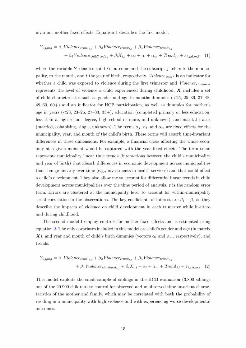
invariant mother fixed-effects. Equation 1 describes the first model:

Yi,j,m,t = β1Violencetrim1 i,j + β2Violencetrim2 i,j + β3Violencetrim3 i,j

+ β4Violencechildhoodi,j+ βiXi,j + αj + αt + αm + Trend j,t + εi,j,d,m,t, (1)

where the variable Y denotes child i’s outcome and the subscript j refers to the munici-

pality, m the month, and t the year of birth, respectively. Violencetrim1 is an indicator for

whether a child was exposed to violence during the first trimester and Violencechildhood

represents the level of violence a child experienced during childhood. X includes a set

of child characteristics such as gender and age in months dummies (<25, 25–36, 37–48,

49–60, 60+) and an indicator for HCB participation, as well as dummies for mother’s

age in years (<23, 23–26, 27–33, 33+), education (completed primary or less education,

less than a high school degree, high school or more, and unknown), and marital status

(married, cohabiting, single, unknown). The terms αj , αt, and αm are fixed effects for the

municipality, year, and month of the child’s birth. These terms will absorb time-invariant

differences in these dimensions. For example, a financial crisis affecting the whole econ-

omy at a given moment would be captured with the year fixed effects. The term trend

represents municipality linear time trends (interactions between the child’s municipality

and year of birth) that absorb differences in economic development across municipalities

that change linearly over time (e.g., investments in health services) and that could affect

a child’s development. They also allow me to account for differential linear trends in child

development across municipalities over the time period of analysis. ε is the random error

term. Errors are clustered at the municipality level to account for within-municipality

serial correlation in the observations. The key coefficients of interest are β1 − β4 as they

describe the impacts of violence on child development in each trimester while in-utero

and during childhood.

The second model I employ controls for mother fixed effects and is estimated using

equation 2. The only covariates included in this model are child’s gender and age (in matrix

X), and year and month of child’s birth dummies (vectors αt and αm, respectively), and

trends.

Yi,j,m,t = β1Violencetrim1 i,j + β2Violencetrim2 i,j + β3Violencetrim3 i,j

+ β4Violencechildhoodi,j+ βiXi,j + αt + αm + Trend j,t + εi,j,d,m,t (2)

This model exploits the small sample of siblings in the HCB evaluation (3.800 siblings

out of the 20.900 children) to control for observed and unobserved time-invariant charac-

teristics of the mother and family, which may be correlated with both the probability of

residing in a municipality with high violence and with experiencing worse developmental

outcomes.

15

4 Results

Table 1 presents summary statistics for all the children and their mothers in the sample,

and by whether they were exposed to zero (29% of the sample), low (22%), or high (49%)

violence in early-life (from in-utero through early childhood). Low violence is defined

as whether a child was exposed to 1 or 2 massacres (between four and nine victims of

massacres) in early-life, while high violence is defined as whether a child was exposed to

more than 2 massacres (or more than nine massacre victims of massacres) in early-life.12

Table 1 shows that 20% of mothers are younger than 23 years of age, 23% are between

23 and 26, and a fifth of the sample is over 33. In terms of education, 31% of mothers have

primary or less, a third has less than a high school diploma, and a third has high school or

more. More than half of mothers cohabitate, 17% are married, and 11% are single. Overall,

Table 1 shows very little differences in maternal characteristics by violence exposure. For

example, 32% of women with children exposed to no violence have primary of less, while

31% and 30% of mothers of children exposed to low or high violence report primary or

less. This suggests that mothers of children exposed to little or high violence in early-life

are similar accross observable dimensions.

In terms of child characteristics, Table 1 shows that 48% of the sample is female,

the average age is 41 months, and 50% of children participate in HCB. The average

HAZ is -1.0, 16% of the sample is stunted, and 3% is severely stunted. Cognitive and

socio-emotional outcomes have been standardized with mean zero. Differences by violence

exposure show that children exposed to violence tend to be older, likely due to the fact

that older children have had more time to be exposed to at least one massacre than

younger children. Thus, I include controls for child’s age in months in all specifications to

account for the correlation between higher age and higher likelihood of experiencing more

massacres. In terms of outcomes, children exposed to high violence are more likely to have

higher HAZ than children exposed to no violence. For example, children exposed to more

than 9 massacre victims over the period from in-utero to current age have an average

height-for-age score of -0.99, while those who were unexposed have a HAZ of -1.05. High-

violence affected children are also less likely to be stunted compared to unexposed children

(by 3 percentage points), and they are more likely to have higher PPVT scores and math

ability than other children (by at least 5 points); however, these children also tend to

have lower verbal ability and higher levels of aggression. In general, these differences are

small and in most cases are not statistically significant. These differences in the raw data

point to the importance of controlling for geographical and temporal sorting in order to

identify the effects of violence on children and families.

12The cut-off of 2 massacres represents the median number of massacres in the full sample. Conclusionsderived from Table 1 are robust to other cutoffs of high and low violence exposure.

16

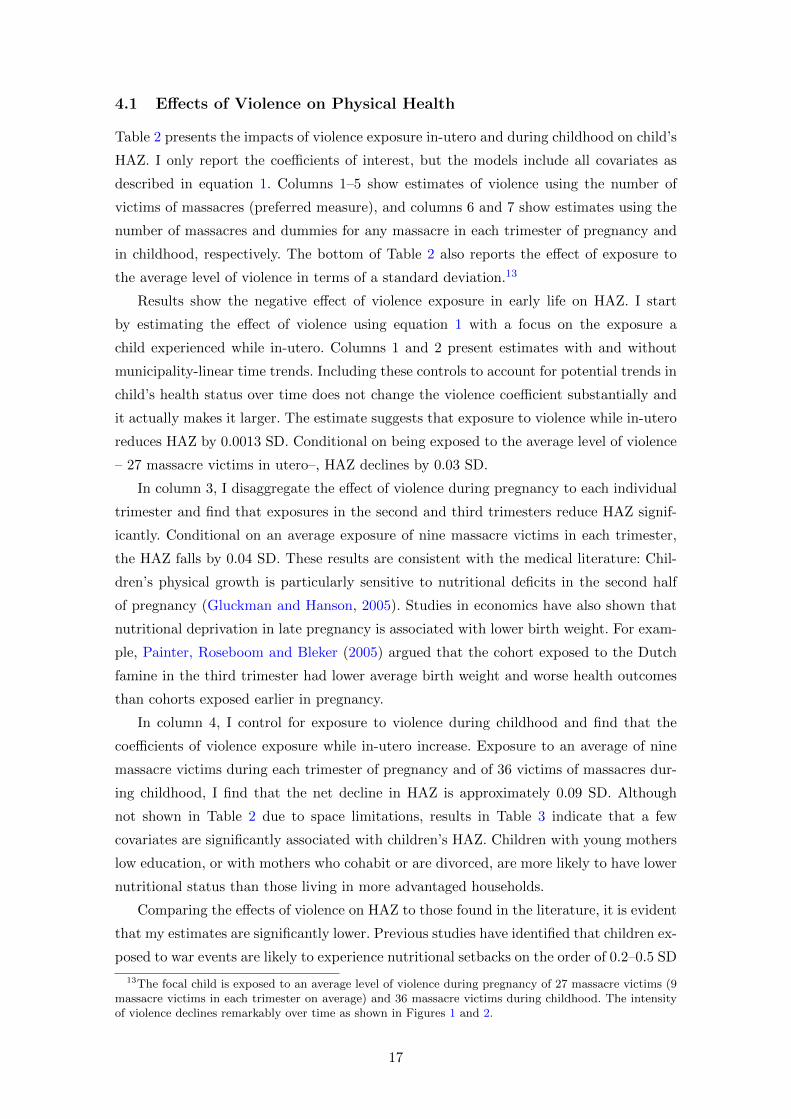
4.1 Effects of Violence on Physical Health

Table 2 presents the impacts of violence exposure in-utero and during childhood on child’s

HAZ. I only report the coefficients of interest, but the models include all covariates as

described in equation 1. Columns 1–5 show estimates of violence using the number of

victims of massacres (preferred measure), and columns 6 and 7 show estimates using the

number of massacres and dummies for any massacre in each trimester of pregnancy and

in childhood, respectively. The bottom of Table 2 also reports the effect of exposure to

the average level of violence in terms of a standard deviation.13

Results show the negative effect of violence exposure in early life on HAZ. I start

by estimating the effect of violence using equation 1 with a focus on the exposure a

child experienced while in-utero. Columns 1 and 2 present estimates with and without

municipality-linear time trends. Including these controls to account for potential trends in

child’s health status over time does not change the violence coefficient substantially and

it actually makes it larger. The estimate suggests that exposure to violence while in-utero

reduces HAZ by 0.0013 SD. Conditional on being exposed to the average level of violence

– 27 massacre victims in utero–, HAZ declines by 0.03 SD.

In column 3, I disaggregate the effect of violence during pregnancy to each individual

trimester and find that exposures in the second and third trimesters reduce HAZ signif-

icantly. Conditional on an average exposure of nine massacre victims in each trimester,

the HAZ falls by 0.04 SD. These results are consistent with the medical literature: Chil-

dren’s physical growth is particularly sensitive to nutritional deficits in the second half

of pregnancy (Gluckman and Hanson, 2005). Studies in economics have also shown that

nutritional deprivation in late pregnancy is associated with lower birth weight. For exam-

ple, Painter, Roseboom and Bleker (2005) argued that the cohort exposed to the Dutch

famine in the third trimester had lower average birth weight and worse health outcomes

than cohorts exposed earlier in pregnancy.

In column 4, I control for exposure to violence during childhood and find that the

coefficients of violence exposure while in-utero increase. Exposure to an average of nine

massacre victims during each trimester of pregnancy and of 36 victims of massacres dur-

ing childhood, I find that the net decline in HAZ is approximately 0.09 SD. Although

not shown in Table 2 due to space limitations, results in Table 3 indicate that a few

covariates are significantly associated with children’s HAZ. Children with young mothers

low education, or with mothers who cohabit or are divorced, are more likely to have lower

nutritional status than those living in more advantaged households.

Comparing the effects of violence on HAZ to those found in the literature, it is evident

that my estimates are significantly lower. Previous studies have identified that children ex-

posed to war events are likely to experience nutritional setbacks on the order of 0.2–0.5 SD

13The focal child is exposed to an average level of violence during pregnancy of 27 massacre victims (9massacre victims in each trimester on average) and 36 massacre victims during childhood. The intensityof violence declines remarkably over time as shown in Figures 1 and 2.

17

in HAZ, compared to similar-aged children not affected by these events (Akresh, Lucchetti

and Thirumurthy, 2012; Minoiu and Shemyakina, 2012; Bundervoet, 2012; Bundervoet,

Verwimp and Akresh, 2009). Two factors might explain the difference in magnitude be-

tween my estimates and those in the literature. First, previous studies have focused on

massive violence episodes such as civil wars or genocides that usually last just a few years,

whereas the Colombian conflict distinguishes from the rest by its long duration and low

intensity, in which civilians have, to some extent, learned how to live under the threat

of armed groups. Second, most previous research has analyzed these impacts in African

countries, in which children, even in the absence of wars or high violence, start from a

lower nutritional baseline, making them more vulnerable to adverse environmental con-

ditions. Compared to studies on the effects of adverse shocks in early life, Rosales (2013)

found that children in Ecuador exposed to the 1998 El Nino weather shock experienced

an average decline in HAZ of 0.09 SD and the negative effect came from exposure during

the third trimester in-utero.

4.1.1 Violence Prior to Conception

In column 5, I include controls for exposure to violence in the two years before conception.

I find little impact of these prior exposures on HAZ that could suggest that preexisting

trends in violence are not driving the results, and thus providing some support for the

validity of the identification strategy.

4.1.2 Changing the definition of violence exposure

In columns 6 and 7, I show results measuring violence using the number of massacres

and dummies for any massacre. Results are remarkably similar to those found in column

4; however, the magnitude of the effect is smaller. Given that the number of victims

of massacres provides greater precision in the intensity of the violence shock than that

captured by the number of massacres or by the dummies for any massacre, I focus the

discussion on this measure in what follows.

4.2 Effects of Violence on Cognitive Outcomes

Table 3 shows estimates of the effect of violence on child cognitive development for those

aged three years and above (sample for whom these outcomes were measured). The re-

sults show that massacre exposure in the first and third trimesters of pregnancy and in

childhood reduce PPVT by 0.15 SD as shown in the bottom row of the Table. Woodcock–

Munoz tests also fall significantly. Verbal ability, math reasoning, and general knowledge

decline by 0.28, 0.19, and 0.16 SD, respectively. Of note is the large effect of violence in

the first trimester of pregnancy, which is consistent with the medical, psychological, and

epidemiological studies that have found that brain development is particularly sensitive

to maternal stress or maternal malnutrition during the first trimester of pregnancy (see

18

discussion in Almond, Mazumder and van Ewijk, 2011; Poggi Davis and Sandman, 2010;

Gluckman and Hanson, 2005). I also find that violence exposure in the second half of

pregnancy has a negative impact on PPVT, verbal ability, and general knowledge, sug-

gesting that changes in the in-utero environment during late pregnancy (e.g., changes in

maternal nutrition) could contribute to these declines. Moreover, the fact that violence

during childhood has a negative impact could be associated with changes in household

dynamics due to the shock.

4.3 Effects of Violence on Socio-emotional Outcomes

Table 4 shows impacts on children’s aggressiveness, withdrawn behavior, and adequate

interaction. The results suggest that violence is associated with higher aggression and

more withdrawn behavior (a positive coefficient of violence on these two outcomes implies

worse child conditions), although the coefficients are not statistically significant at the

0.95 level; I do find, however, a statistically significant and negative relationship between

massacre exposure in early childhood and adequate interaction (the coefficient is −0.04

SD). This effect is smaller than that in Sharkey et al. (2012), who found that children

assessed within a week of a homicide occurring near their home exhibited 0.33 SD lower

levels of attention and impulse control. It is possible that the smaller effects are due to

the timing in the shock (I consider a much longer time frame, from the prenatal period

up to a maximum of age 7) and the fact that this study considers indirect exposure to

violence at the municipality level.

4.4 Heterogeneous results

4.4.1 Results by Gender

Studies investigating the impacts of early-life shocks on child outcomes have found that

girls tend to suffer more than boys (Rose, 1999; Shemyakina, 2011; Akresh, Lucchetti

and Thirumurthy, 2012). In this study, I explore differences in the effects of massacre

exposure by gender and find that, consistent with previous studies, girls are more likely

to experience larger physical and socio-emotional developmental setbacks than boys. The

results presented in Table 5 show that girls who are exposed to violence in early life

achieve 0.013 SD lower height and a 0.05 SD worse adequate interaction than similarly

exposed boys (although this last coefficient is not statistically significant at the 0.95

level). Boys, in contrast, experience no change in these outcomes. In terms of cognitive

development, I do find a stronger decline on PPVT among boys (-0.17 versus −0.07 SD

among girls) which is mainly driven by childhood exposure to violence. Although not

shown here due to space limitations, I also find that girls experience a more negative

impact on other cognitive outcomes such as math reasoning (-0.35 SD versus no effect on

boys) and general knowledge about the world (-0.37 SD versus no effect on boys).

19

Based on these results, a reasonable question to ask would be, Can these impacts be

driven by child (i.e., male) selective mortality? I examine the possibility of this threat

in the robustness-checks section and find little evidence that violence is endogenously

affecting mortality. Hence, the fact that I find differential impacts across boys and girls

could reflect, to some extent, endogenous parental investments within households that

may be favoring boys over girls.

4.4.2 Results by Household Socioeconomic Status

A recurring empirical finding is that low-socioeconomic (SES) families are more likely to

experience more and more persistent shocks (Currie and Hyson, 1999; Currie and Vogl,

2013). If the effects of violence differ across family SES, this could suggest that some

families are more or less likely to protect their children from them. Table 6 shows results

by mother’s education. I estimate models in which I split the sample by whether the

mother has less than a secondary education (the median schooling in the sample) versus

secondary or more. I find that children of less and more educated mothers experience a

similar decline in HAZ (the overall decline is approximately 0.5 SD and the differences

are not statistically significant across samples). Violence, however, exerts a larger toll

on cognitive and socio-emotional development among children of less educated mothers:

PPVT and adequate interaction fall by 0.23 and 0.05 SD, respectively, whereas no change

is observed among children in more affluent families.

4.4.3 Results by Violence Exposure

I now estimate results by the magnitude of the shock: small versus large massacres. I first

exclude children who had not experienced massacres in early-life (29% of the sample), and

then I split the sample by those who experienced low violence (less than 3 masscres or

between 4 and 9 massacre victims) and high violence (more than 2 massacres or more than

9 massacre victims). Table 7 shows results and these suggest that the effects of violence

on child‘s HAZ are exclusively driven by those who were exposed to large massacres. This

result is consistent with the idea that only shocks that are more impactfull are likely to

have significant effects on children.

4.5 Sibling Fixed-Effects Models

One potential threat to my empirical specification occurs if mothers of certain character-

istics are more likely to be impacted by violence and are also more likely to have children

with worse developmental outcomes. If this were the case, the estimates of violence ob-

tained using equation 1 could be overestimating the true impact. To explore whether the

results could be driven by a mother’s unobserved characteristics, I exploit the small sam-

ple of siblings in the HCB data (there are 3,816 siblings among the 20,936 children) using

equation 2.

20

Table 8 shows sibling fixed effects of violence on HAZ. Column 3 indicates that an

increase in violence in the third trimester of pregnancy reduces children’s HAZ by 0.05

SD; this result is smaller to that obtained in column 2 using the linear specification for

the sample of siblings (N = 3,816) (0.05 versus 0.17 SD, respectively), but it describes

a similar pattern. In other words, the fact that I obtain similar results with and without

mother fixed effects suggests that violence does not seem to be correlated with a mother’s

time-invariant unobserved characteristics, providing support for the identification strat-

egy.

Column 3 in Table 9 shows fixed-effects estimates on children’s PPVT and these show

that, exposures in the first and third trimester are negatively associated with this outcome.

The overall effect of violence is actually twice the size of that in the full sample (estimate

in 3 is 0.032 SD and in column 1 is 0.017 SD). Similarly, Column 3 in Table 10 shows

estimates of violence on child’s adequate interaction. I find that although the estimate

of violence in childhood is similar in magnitude (-0.0010), this coefficient did not reach

statistical significance likely due to a power issue.

4.6 Fetal Health

Health at birth is a key input in the production of human capital (Heckman, 2008). Birth

weight is a summary measure of initial endowments that may capture prenatal investments

(Bharadwaj, Eberhard and Neilson, 2013; Rosenzweig and Zhang, 2009), and is a strong

predictor of future outcomes such as educational attainment and health (Black, Devereux

and Salvanes, 2007; Currie and Hyson, 1999).

Previous studies have shown that violence exposure during pregnancy negatively af-

fects health at birth outcomes. Camacho (2008) found that pregnant mothers exposed to

landmine explosions in Colombia give birth to babies who are 8.7 grams less heavy. Using

data from Palestine, Mansour and Rees (2012) found a small increase in the incidence of

low birth weight (Brown, 2014), for the case of Mexico, found that exposure to the average

increase in local homicide rates was associated with a decline in birth weight of 75 grams

and a 40% increase in in the probability of low birth weight. These authors found the

strongest impacts of violence shocks in the first trimester of pregnancy. I examine whether

the measure of violence used in this study provides estimates consistent with those found

in the literature. I do so by regressing the baseline specification14 and using data from

Vital Statistics Birth Records, which has been widely used in previous studies of fetal

health and provides a large sample of births.15

14In addition to basic characteristics (child’s gender and mother’s age, education, and relationshipstatus), models control for multiple birth, parity, urban household, whether the baby was delivered at ahospital, and whether the mother had medical insurance (public, private, other). They also include thechild’s month, year, and municipality of birth fixed effects.

15HCB does not provide health at birth outcomes. Unfortunately, I do not have access to mother’sidentifiers to estimate mother fixed-effects models by comparing siblings. I pool years 1998–2001 and2005–2006. Years 2002–2004 were not included since they were not available to the author when theseanalyses were performed. The total sample includes approximately 4 million births across all municipalities

21

Table 11 shows a small but negative effect of violence on birth weight in the first

trimester of pregnancy. Conditional on an average exposure to nine massacre victims in

the first trimester, birth weight falls by 1.3 grams. This effect is larger for less educated

mothers (those with primary education or less) than for the more educated (2.4 versus 1.4

grams, respectively) and provides some evidence consistent with the idea that maternal

stress could be an important channel through which violence impacts child outcomes

(Aizer, Stroud and Buka, 2012; Denckel-Schetter, 2011).

4.7 Potential Mechanisms: Parental Investments

In this section, I explore whether violence shocks affect parental investments. Table 12

presents summary statistics on these measures for the full sample and by whether children

were exposed to high versus low violence in early life (as defined in Table 1). Overall,

I find little differences in prenatal care, breastfeeding, child vaccinations, and protein

servings across children exposed to high and low violence. In terms of parenting, however,

differences suggest that those more likely to have experienced high violence tend to receive

less maternal time and more physical and psychological aggression. Interestingly, these

children are also more likely to have mothers who invest more time in activities that

stimulate their cognitive potential.

I use equation 1 to investigate the associations between in-utero and childhood violence

and parental investments and results are shown in Tables 13 and 14.16 Results show little

evidence that changes in violence are associated with changes in parental investments.

For instance, I find no significant association between changes in violence and changes in

prenatal care, breastfeeding, child vaccination, or protein consumption. Moreover, results

show that higher violence (in-utero and in childhood) is associated with more frequent

psychological aggression but little change in other measures.

4.8 Heterogeneous results

4.8.1 Results by Child’s Age

Given that parental investments can vary considerably depending on a child’s age and

that younger children are more likely to have been exposed to more recent violence shocks

(i.e., the in-utero period for younger children is closer to the interview date than that for

older children), I show associations separately for young (up to three years) versus older

children (three or more years).

The second and third panel of Table 13 show differences by age. I find that younger

children are less likely to receive prenatal care (by 3.3% with the average exposure to

massacres) while older children experience a mild reduction in breastfeeding (-0.4%) and in

in Colombia.16Due to the small variation in siblings in the HCB data, I do not estimate sibling fixed-effects models

to investigate the effects of violence on potential mechanisms.

22

the number of protein servings received in the last week (-1%). Given the small magnitude

in the coefficients and the fact that results are only significant for young kids, these results

suggest that violence is not related to the provision of medical services at the local level.

Turning to parenting indicators, Table 14 reveals that among children under three

years old there is a decline in the number of hours a mother spends with her child (by

almost one hour per week which is equivalent to an 11% decline with respect to the mean)

and a decline in the frequency of routines that stimulate a child’s cognitive development

(0.12 SD or 10.4%); I also find that violence-exposed mothers are more likely to be psy-

chologically aggressive with their children (0.12 SD or 18.2%). The findings for the older

cohorts show little impacts of violence on parenting outcomes, which could be due to

parents responding to violence in the short-term but not necessarily changing their be-

havior in the long-term. In sum, Tables 13 and 14 suggest that parents whose children

are exposed to massacre shocks in their early life are more likely to reinforce the negative

impacts of the shock by reducing the quantity and quality of their investments; however,

this result is rather consistent with the hypothesis that parents may prefer equality across

children.

4.9 Potential for Remediation

A growing body of evidence documents the persistent effects of early-life shocks on socio-

economic outcomes; but whether these effects can be mitigated with interventions remains

largely unexplored (Almond and Mazumder, 2013). From a policy perspective this ques-

tion is of great interest considering that resources are often limited and shocks are more

frequent among disadvantaged subpopulations. Few studies have provided empirical find-

ings on whether social programs can compensate for early-life shocks and the evidence is

so far mixed.17

In this section, I explore whether HCB can help remediate the negative effects of vio-

lence on children. In principle, one would expect that HCB would have mitigating impacts

on children since HCB helps promote their physical, cognitive, and social development

and supports healthy parenting.18 But, the extent to which the program helps overcome

the deficits between children exposed and unexposed to violence is a priori not clear.

A credible evaluation of the potential for remediation of HCB would ideally use a ran-

17Aguilar and Vicarelli (2012) found that Progresa, the Mexican conditional cash transfer programavailable for low-income households, was unable to mitigate the effects of extreme weather shocks onchildren’s health and cognitive development. In contrast, Adhvaryu et al. (2014) focusing on rainfall shocksand on the mitigating role of Progresa, actually found that cash transfers helped remediate the effect ofextreme rainfall on educational outcomes, by almost 60 percent. Gunnsteinsson, Snaebjorn, Adhvaryu,Christian, and Labrique (2014) found that a maternal and newborn vitamin A supplementation programreduced the effects of a tornado in Bangladesh. They found that not only were babies who receive vitaminA more robust after the tornado in terms of their anthropometric indicators as compared to exposedbabies who did not receive vitamin A, but there was also full catch-up.

18Each HCB center serves up to 15 children between the ages of 6 months to 7 years in part-time orfull-time schedules during weekdays. These centers are led by a communitarian mother who is a home-based childcare provider in the same community, and parents contribute with a maximum monthly fee of25 percent of the daily minimum wage (Bernal et al., 2009).

23

domized control trial that randomly assigns children to a treatment and a control group.

However, this is challenging because HCB is by now so widespread.19 One way to address

the potential problem of selection into the program is through instrumental variables. At-

tanasio, Di Maro, and Vera-Hernandez (2013) instrumented HCB participation and HCB

exposure with indicators for the availability of HCB in the local community. In particular,

one of their instruments was the distance from a household to the closest HCB center.20

I build on Attanasio et al., (2013) by using distance and distance squared from the

residence to the nearest HCB (in kilometers) as instrumental variables for HCB expo-

sure.21 Appendix Table B8 shows that distance is an important determinant for children‘s

participation in HCB and children‘s duration into the program, but not so among non-

participant children. Therefore, I conduct the IV analysis on the sample of children who

participate in HCB (and exludes the non-participants) and I focus on program exposure

(duration) rather than on program participation. I create a dummy variable that takes

the value of one for children who have been in the program for more than the median

program exposure, 13 months, and zero for children who have participated 13 months or

less. Since I am interested in the heterogenous effect that HCB could have on children

who were exposed to different levels of violence in their lives (i.e., remediation potential),

I include an interaction term between HCB exposure and violence. I also estimate a first

stage regression for this interaction term. Equations 3, 4, and 5 describe the first and

second stages of my instrumental variables approach that I estimate using a two-stage

least squares (2SLS):

First stages:

HCB exposurei,j,m,t = β0 + βdDistancei,t + βd2Distance2i,t+

+βdvDistancei,t × V iolencei,t + βd2vDistance2i,t × V iolencei,t+

βvV iolence,i,t + γXi,j + αj + αm + αt + εi,j,m,t (3)

HCB exposure× V iolencei,j,m,t = β0 + βdDistancei,t + βd2Distance2i,t+

+βdvDistancei,t × V iolencei,t + βd2vDistance2i,t × V iolencei,t+

βvV iolence,i,t + γXi,j + αj + αm + αt + εi,j,m,t (4)

19Bernal and Fernandez (2013) showed that HCB participants were more disadvantaged in terms ofhousehold income, having an absent father, and mothers age than non-participants.

20This study used distance as an instrumental variable in their analysis with rural households, those forwhom distance to the nearest HCB can be a more important determinant of HCB exposure. Using thisIV approach, they found that HCB participation and HCB exposure increased a child’s HAZ by 0.8 to1.2 SD.

21Instrumenting HCB exposure with distance and distance squared I find that HCB has a positiveimpact on child‘s HAZ of 0.49 SD whereas Attanasio et al., (2013) found effects between 0.8 and 1..2 SD.

24

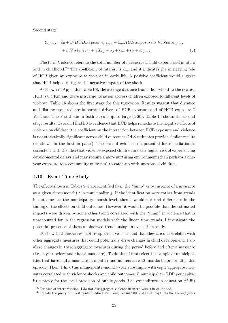
Second stage:

Yi,j,m,t =β0 + βh ˆHCB exposurei,j,m,t + βhv ˆHCB exposure× V iolencei,j,m,t

+ βvV iolencei,t + γXi,j + αj + αm + αt + εi,j,m,t (5)

The term Violence refers to the total number of massacres a child experienced in utero

and in childhood.22 The coefficient of interest is βhv and it indicates the mitigating role

of HCB given an exposure to violence in early life. A positive coefficient would suggest

that HCB helped mitigate the negative impact of the shock.

As shown in Appendix Table B8, the average distance from a household to the nearest

HCB is 0.4 Km and there is a large variation accross children exposed to different levels of

violence. Table 15 shows the first stage for this regression. Results suggest that distance

and distance squared are important drivers of HCB exposure and of HCB exposure *

Violence. The F-statistic in both cases is quite large (>20). Table 16 shows the second

stage results. Overall, I find little evidence that HCB helps remediate the negative effects of

violence on children: the coefficient on the interaction between HCB exposure and violence

is not statistically significant across child outcomes. OLS estimates provide similar results

(as shown in the bottom panel). The lack of evidence on potential for remediation is

consistent with the idea that violence-exposed children are at a higher risk of experiencing

developmental delays and may require a more nurturing environment (than perhaps a one-

year exposure to a community nurseries) to catch-up with unexposed children.

4.10 Event Time Study

The effects shown in Tables 2–9 are identified from the “jump” or occurrence of a massacre

at a given time (month) t in municipality j. If the identification were rather from trends

in outcomes at the municipality–month level, then I would not find differences in the

timing of the effects on child outcomes. However, it would be possible that the estimated

impacts were driven by some other trend correlated with the “jump” in violence that is

unaccounted for in the regression models with the linear time trends. I investigate the

potential presence of these unobserved trends using an event time study.

To show that massacres capture spikes in violence and that they are uncorrelated with

other aggregate measures that could potentially drive changes in child development, I an-

alyze changes in these aggregate measures during the period before and after a massacre

(i.e., a year before and after a massacre). To do this, I first select the sample of municipal-

ities that have had a massacre in month t and no massacre 12 months before or after this

episode. Then, I link this municipality–month–year subsample with eight aggregate mea-

sures correlated with violence shocks and child outcomes: i) municipality–GDP per capita;

ii) a proxy for the local provision of public goods (i.e., expenditure in education);23 iii)

22For ease of interpretation, I do not disaggregate violence in utero versus in childhood.23I create the proxy of investments in education using Census 2005 data that captures the average years

25

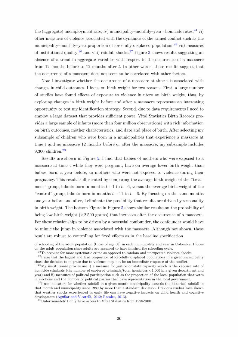
the (aggregate) unemployment rate; iv) municipality–monthly–year - homicide rates;24 vi)

other measures of violence associated with the dynamics of the armed conflict such as the

municipality–monthly–year proportion of forcefully displaced population;25 vii) measures

of institutional quality;26 and viii) rainfall shocks.27 Figure 3 shows results suggesting an

absence of a trend in aggregate variables with respect to the occurrence of a massacre

from 12 months before to 12 months after t. In other words, these results suggest that

the occurrence of a massacre does not seem to be correlated with other factors.

Now I investigate whether the occurrence of a massacre at time t is associated with

changes in child outcomes. I focus on birth weight for two reasons. First, a large number

of studies have found effects of exposure to violence in utero on birth weight, thus, by

exploring changes in birth weight before and after a massacre represents an interesting

opportunity to test my identification strategy. Second, due to data requirements I need to

employ a large dataset that provides sufficient power: Vital Statistics Birth Records pro-

vides a large sample of infants (more than four million observations) with rich information

on birth outcomes, mother characteristics, and date and place of birth. After selecting my

subsample of children who were born in a municipalities that experience a massacre at

time t and no massacre 12 months before or after the massacre, my subsample includes

9,300 children.28

Results are shown in Figure 5. I find that babies of mothers who were exposed to a

massacre at time t while they were pregnant, have on average lower birth weight than

babies born, a year before, to mothers who were not exposed to violence during their

pregnancy. This result is illustrated by comparing the average birth weight of the “treat-

ment“ group, infants born in months t+ 1 to t+ 6, versus the average birth weight of the

“control“ group, infants born in months t− 11 to t− 6. By focusing on the same months

one year before and after, I eliminate the possibility that results are driven by seasonality

in birth weight. The bottom Figure in Figure 5 shows similar results on the probability of

being low birth weight (<2,500 grams) that increases after the occurrence of a massacre.

For these relationships to be driven by a potential confounder, the confounder would have

to mimic the jump in violence associated with the massacre. Although not shown, these

result are robust to controlling for fixed effects as in the baseline specification.

of schooling of the adult population (those of age 30) in each municipality and year in Colombia. I focuson the adult population since adults are assumed to have finished the schooling cycle.

24To account for more systematic crime as opposed to random and unexpected violence shocks.25I also test the lagged and lead proportion of forcefully displaced populations in a given municipality

since the decision to migrate due to violence may not be an immediate response of the conflict.26My institutional proxies are i) a measure for justice or state capacity which is the capture rate of

homicide criminals (the number of captured criminals/total homicides× 1,000 in a given department andyear) and ii) measures of political participation such as the proportion of the local population that votesin elections and the number of political parties that have representation in the local government.

27I use indicators for whether rainfall in a given month–municipality exceeds the historical rainfall inthat month and municipality since 1980 by more than a standard deviation. Previous studies have shownthat weather shocks experienced in early life can have negative impacts on child health and cognitivedevelopment (Aguilar and Vicarelli, 2012; Rosales, 2013).

28Unfortnunately I only have access to Vital Statistics from 1998-2001.

26

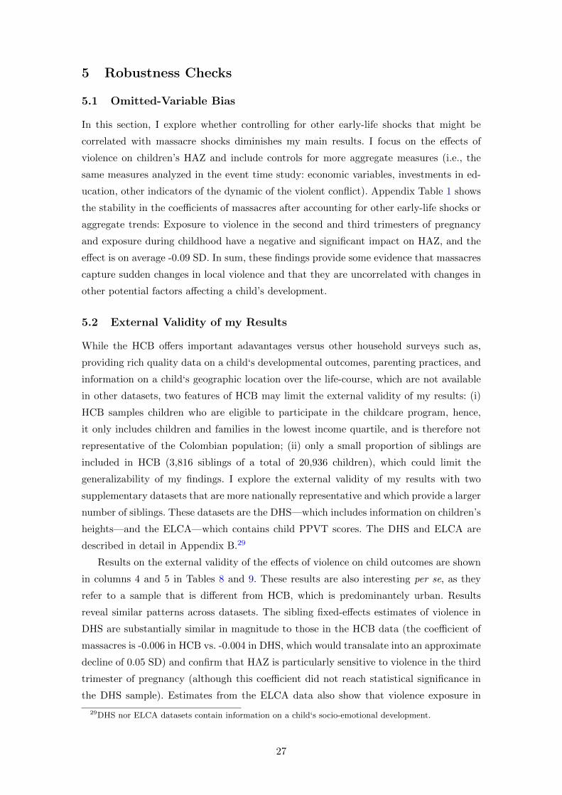
5 Robustness Checks

5.1 Omitted-Variable Bias

In this section, I explore whether controlling for other early-life shocks that might be

correlated with massacre shocks diminishes my main results. I focus on the effects of

violence on children’s HAZ and include controls for more aggregate measures (i.e., the

same measures analyzed in the event time study: economic variables, investments in ed-

ucation, other indicators of the dynamic of the violent conflict). Appendix Table 1 shows

the stability in the coefficients of massacres after accounting for other early-life shocks or

aggregate trends: Exposure to violence in the second and third trimesters of pregnancy

and exposure during childhood have a negative and significant impact on HAZ, and the

effect is on average -0.09 SD. In sum, these findings provide some evidence that massacres

capture sudden changes in local violence and that they are uncorrelated with changes in

other potential factors affecting a child’s development.

5.2 External Validity of my Results

While the HCB offers important adavantages versus other household surveys such as,

providing rich quality data on a child‘s developmental outcomes, parenting practices, and

information on a child‘s geographic location over the life-course, which are not available

in other datasets, two features of HCB may limit the external validity of my results: (i)

HCB samples children who are eligible to participate in the childcare program, hence,

it only includes children and families in the lowest income quartile, and is therefore not

representative of the Colombian population; (ii) only a small proportion of siblings are

included in HCB (3,816 siblings of a total of 20,936 children), which could limit the

generalizability of my findings. I explore the external validity of my results with two

supplementary datasets that are more nationally representative and which provide a larger

number of siblings. These datasets are the DHS—which includes information on children’s

heights—and the ELCA—which contains child PPVT scores. The DHS and ELCA are

described in detail in Appendix B.29

Results on the external validity of the effects of violence on child outcomes are shown

in columns 4 and 5 in Tables 8 and 9. These results are also interesting per se, as they

refer to a sample that is different from HCB, which is predominantely urban. Results

reveal similar patterns across datasets. The sibling fixed-effects estimates of violence in

DHS are substantially similar in magnitude to those in the HCB data (the coefficient of

massacres is -0.006 in HCB vs. -0.004 in DHS, which would transalate into an approximate

decline of 0.05 SD) and confirm that HAZ is particularly sensitive to violence in the third

trimester of pregnancy (although this coefficient did not reach statistical significance in

the DHS sample). Estimates from the ELCA data also show that violence exposure in

29DHS nor ELCA datasets contain information on a child‘s socio-emotional development.

27

the first trimester significantly reduces a child’s PPVT and the overall effect of violence is

much larger than that found in the HCB data (-0.53 SD in ELCA vs. -0.21 SD in HCB).

In general, the effects of violence found in Tables 8 and 9 suggest that estimates are not

specific to a certain subpopulation of children and that they are in fact highly consistent

across specifications with and without a mother fixed-effect, which may suggest that the

occurrence of massacres at the monthly, year, and municipality levels is uncorrelated with

household characteristics.

5.3 Potential Sources of Selection Bias

A complicating factor in the study of the impacts of violence on child outcomes is that

violence may not only have a scarring effect on affected cohorts, but may also induce

selection through sorting, migration, fertility, or mortality (Almond, 2006; Valente, 2013;

Bozzoli, Deaton and Quintana-Domeque, 2009). In this paper, I carefully explore whether

the effects of violence on children are driven by these potential sources of selection bias.

For this purpose, I complement some of these analyses in the HCB data with several

waves of the DHS and the Colombian population Census 2005 that provide a much larger

sample of births at the municipality level, allowing me to explore these concerns in more

detail.30

5.4 Geographic Sorting

Families living in conflict-prone municipalities may also be disadvantaged in other di-

mensions. For instance, they may be less educated compared to families in municipalities

unaffected by violence. To account for these differences across municipalities, I include

birth municipality, year, and month fixed effects. However, if these differences are likely

to change over time, or if there are differences in terms of who is affected by violence

within municipalities, then, even after controlling for fixed effects, there will be selective

sorting within areas. Since violence often leads to disruption in the local conditions, this

issue may be particularly important.

To test for the presence of selective sorting within Colombian municipalities, I com-

pare the characteristics of mothers who were exposed to violence during pregnancy and

during their child’s early childhood to mothers who were not exposed. In the presence of

selective sorting, the association between a mother’s characteristics and the occurrence

of massacres should be significant even after accounting for municipality fixed effects. To

30The Census 2005 (N = 4 million individuals, accounting for 10% of the total population) has thevirtue that it reports the municipality and date of birth for each individual, and the municipality wherea mother lived when she was pregnant. This information enables me to identify the level of violenceto which each individual was exposed in each trimester of pregnancy. I obtain Census 2005 data fromIPUMS-International.

28

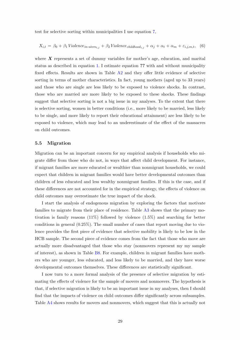
test for selective sorting within municipalities I use equation 7,

Xi,t = β0 + β1Violence in-uteroi,j + β2Violencechildhoodi,j+ αj + αt + αm + εi,j,m,t, (6)

where X represents a set of dummy variables for mother’s age, education, and marital

status as described in equation 1. I estimate equation ?? with and without municipality

fixed effects. Results are shown in Table A2 and they offer little evidence of selective

sorting in terms of mother characteristics. In fact, young mothers (aged up to 33 years)

and those who are single are less likely to be exposed to violence shocks. In contrast,

those who are married are more likely to be exposed to these shocks. These findings

suggest that selective sorting is not a big issue in my analyses. To the extent that there

is selective sorting, women in better conditions (i.e., more likely to be married, less likely

to be single, and more likely to report their educational attainment) are less likely to be

exposed to violence, which may lead to an underestimate of the effect of the massacres

on child outcomes.

5.5 Migration

Migration can be an important concern for my empirical analysis if households who mi-

grate differ from those who do not, in ways that affect child development. For instance,

if migrant families are more educated or wealthier than nonmigrant households, we could

expect that children in migrant families would have better developmental outcomes than

children of less educated and less wealthy nonmigrant families. If this is the case, and if

these differences are not accounted for in the empirical strategy, the effects of violence on

child outcomes may overestimate the true impact of the shock.

I start the analysis of endogenous migration by exploring the factors that motivate

families to migrate from their place of residence. Table A3 shows that the primary mo-

tivation is family reasons (11%) followed by violence (1.5%) and searching for better

conditions in general (0.25%). The small number of cases that report moving due to vio-

lence provides the first piece of evidence that selective mobility is likely to be low in the

HCB sample. The second piece of evidence comes from the fact that those who move are

actually more disadvantaged that those who stay (nonmovers represent my my sample

of interest), as shown in Table B8. For example, children in migrant families have moth-

ers who are younger, less educated, and less likely to be married, and they have worse

developmental outcomes themselves. These differences are statistically significant.

I now turn to a more formal analysis of the presence of selective migration by esti-

mating the effects of violence for the sample of movers and nonmovers. The hypothesis is

that, if selective migration is likely to be an important issue in my analyses, then I should

find that the impacts of violence on child outcomes differ significantly across subsamples.

Table A4 shows results for movers and nonmovers, which suggest that this is actually not

29

the case; the effect of violence is almost identical in the two cases.

5.6 Fertility

Violence may also affect fertility decisions in terms of family size or pregnancy timing.

If violence has a differential impact on fertility across women’s characteristics, then, it

is likely that the estimates of violence on child outcomes may be biased, as the sample

of children (on whom I estimate these effects) could be a selected sample. For instance,

if violence reduces fertility incentives only for the most educated, wealthy, and healthy

women, then, those women more likely to become pregnant would tend to be a more

disadvantaged group and their children would be, on average, more likely to have worse

developmental outcomes even in the absence of violence.

To test for the presence of selective fertility, I examine whether violence shocks are

associated with a woman’s fertility decisions across observable characteristics, and I use

DHS data that provides rich information on both family size and timing of fertility.31 I

measure total fertility using the number of children that have been born after a given

child (focal child), and the timing of fertility is measured using both the succeeding birth

interval (in months) after the focal child and the preceding birth interval (in months)

before the focal child. I use equation 7 describes to test for this type of selection,

Ym,t = β0 + β1Violence in-uteroi,j + β2Violence in-uteroi,j ∗Xi,j

+ β3Xi,j + αj + αt + αm + εi,j,m,t, (7)

where Y is the outcome measured as a continuous variable; X represents the mother’s

characteristics; the term Violence indicates the number of massacre victims to which

the mother’s focal child was exposed to in early life; the interactions between violence

and mother characteristics capture whether fertility was selective on a specific maternal

characteristic.

The results shown in Table A5 offer little evidence for selective fertility on observable

mother characteristics. The associations between violence in-utero and up to age three

years, and total fertility and timing of fertility are not statistically significant and most

of the interaction terms between violence and mother controls are zero.

5.7 Survival

The estimates of early-life shocks may also be affected by selection on survival both

at birth and during childhood: Violence is likely to increase the chances of dying for

those with weaker health endowment (see, for example, Almond, 2006). To test how

massacres affect survival, I provide some evidence on how changes in violence affect a

child’s mortality in the first month, year, and three years of life. I use DHS data and

31Unfortunately, the HCB data do not include information on fertility.

30

I estimate a model similar to equation 7. Table A6 shows that neither the associations

between violence and child’s mortality nor the interactions between violence and mother’s

characteristics are statistically significant. Of note, however, is that these results are

conditional on both child and mother survival in 2000 and 2005, and on children living

in the same household with their mothers.

Lastly, I investigate how violence in-utero affects the cohort size and the sex ratio

using census data. I examine the relationship between violence and the sex ratio because

several studies have indicated that boys are biologically weaker and more susceptible to

diseases and premature death than girls (Naeye et al., 1971; Waldron, 1985), and that

they are more vulnerable to environmental factors (Pongou, 2013). Hence, looking at how

violence affects the sex ratio is also informative of the presence of selective survival.

If violence is increasing the chances of dying at birth or later, I expect to find a

negative association between violence and the cohort size and sex ratio. Cohort size is

defined as the total number of births born in each municipality–year for those who, by

year 2005, were between three and six years of age.32 Sex ratio is defined as the number

of boys divided by the number of girls born in each municipality–year.

Yj,t = β0 + βtViolence in-uteroi,j + αj + αt + εj,t (8)

I regress municipality–year cohort size on the violence that children experienced in-utero

as shown by equation 8. Table A7 shows the associations between violence and the cohort

size and sex ratio for all the municipalities in Colombia and for those sampled in the HCB

evaluation. These results indicate that neither the cohort size nor the sex ratio is signifi-

cantly associated with changes in violence, suggesting that these estimates of violence on

child outcomes are not driven by selective mortality. These findings are consistent with

a number of studies documenting no effect of in-utero violence on the sex ratio (Polasek

et al., 2005).

6 Concluding Remarks

The foundations of later-life success are mostly built in the early years. Children exposed

to adverse conditions in-utero and in childhood start behind and in the absence of inter-

ventions that help even out opportunities, inequality in the future will be reinforced. This

paper contributes to the literature by estimating the effects of early-life shocks on three

dimensions of human capital formation—child’s health and cognitive and socio-emotional

development, three strong predictors of future socioeconomic outcomes. I focus on vio-

lence that represents a significant shock to the well-being of many households, reaching

beyond direct victims through its effects on stress, health, and economic resources. Results

32Results are robust to focusing on the period of childhood exclusively or on the period that combinesin-utero and in childhood. I focus on the in-utero period here for presentation purposes.

31

show that violence shocks in early life significantly reduce a child’s nutritional status and

cognitive and non-cognitive development. The evidence on potential mechanisms suggests

that violence reduces parental investments such as the duration of breastfeeding and food

consumption. Lastly, I explore changes in parental quality and find that violence is associ-

ated with a decline in the time mothers spend with their child, a decrease in the frequency

of routines that stimulate a child’s cognitive development, and an increase in psycholog-

ical aggression, which could reflect the presence of maternal stress. To my knowledge,

this is the first paper to provide evidence on parenting as a potential pathway by which

community violence affects children.

The declines in child’s health and cognitive development can be translated into future

wage declines. Following the discussion in Vogl (2012) for nutritional status33 in Mexico,

in Alderman et al. (1996) for cognitive ability34 in Pakistan, and in Heckman, Stixrud

and Urzua (2006) for socio-emotional skills in the United States, I find that children

in Colombia are likely to experience a 2.4%, a 3.4%, and a 0.4% decline in their wages

due to the effects of violence on HAZ and on cognitive and non-cognitive development,

respectively.

My results have important implications for public policy. First, while children can be

permanently damaged in the early ages, if adequate interventions are adopted, these effects

could be mitigated. One example of such policies would be to ensure adequate nutrition

for women of childbearing age and for young children. Second, social protection programs

that have been shown to improve poor families’ coping strategies against many adversities

could also help improve violence-exposed families’ financial, physical, and psychological

well-being. Third, policies that foster children’s potential—for example, high-quality early

childhood education or interventions that help promote positive parenting practices or

home-visiting policies—could also have important benefits for children and families.35

This study faced several limitations. First, as in many developing countries, the data

available are cross-sectional and so scientists face multiple challenges in providing convinc-

ing evidence of a causal relationship. For example, one particular concern in this study

is whether the age patterns between ages one to three years and ages four to seven years

may in part be driven by differences in the two age-group samples rather than by violence

exposure. Second, although this paper provided some evidence on potential pathways

through which a violence shock could have affected child outcomes, I was not able to test

whether violence was associated with changes in household income, an important pathway

that is likely to be associated with parenting behavior and child investments. Third, the

socio-emotional measures (Penn Interactive Peer Play Scale for agression, isolation, and

adequate interaction) are designed to evaluate a child‘s socio-emotional development while

33The author finds that an extra centimeter of height is associated with 2.5% higher wages.34The authors find that a one-standard deviation increase in cognitive achievement implies an increase

in wages of over 20%.35Recent research has shown that psychosocial stimulation provided to poor families with young children

significantly improved children’s psychosocial skills (Gertler et al., 2013).

32

peer play and not more genrally or in other contexts. Future research should examine the

role of potential channels of transmission in more detail. While this study provides some

evidence that violence deteriorates parenting practices, which is consistent with a high

incidence of maternal stress and depression, I do not test this association. The relation-

ship between violence and mothers’ mental health represents an important mechanism

due to the high prevalence of violent conflicts around the world and the well-established

negative link between mothers’ depression and child development. Moreover, studies that

further explore whether violence affects parental child-gender preferences is an important

area of research as it could represent a new pathway through which violence reinforces

gender inequality.

33

References

Adhvaryu, A., T. Molina, A. Nyshadham, and J. Tamayo 2014. “Recovering

from Early Life Trauma: Dynamic Substitution between Child Endowments and In-

vestments.” Working paper.

Aguilar, A., and M. Vicarelli. 2012. “El Nino and Mexican Children: Medium-Term

Effects of Early-Life Weather Shocks on Cognitive and Health Outcomes.” Working

paper.

Aizer, A., and F. Cunha. 2014. “Child Endowments, Parental Investments and the

Production of Human Capital.” National Bureau for Economic Research wp#18429.

Aizer, A., L. Stroud, and S. Buka. 2012. “Maternal Stress and Child Outcomes:

Evidence from Siblings.” National Bureau for Economic Research 18422.

Akbulut-Yuksel, M. 2009. “Children of the War: The Long-Run Effects of Large Scale

Physical Destruction and Warfare on Children.” Institute for the Study of Labor Dis-

cussion paper 4407.

Akresh, R., and D. de Walque. 2011. “Armed Conflict and Schooling: Evidence from

the 1994 Rwandan Genocide.” World Bank.

Akresh, R., L. Lucchetti, and H. Thirumurthy. 2012. “Wars and Child Health:

Evidence from the Eritrean-Ethiopian Conflict.” Journal of Development Economics,

99: 330–340.

Alderman, H., J. Behrman, D. Ross, and R. Sabot. 1996. “The Returns to En-

dogenous Human Capital in Pakistan’s Rural Wage Labour Market.” Oxford Bulletin

of Economics and Statistics, 58(1): 29–55.

Almond, D. 2006. “Is the 1918 Influenza Pandemic Over? Long-Term Effects of in Utero

Influenza Exposure in the Post-1940 U.S. Population.” Journal of Political Economy,

114(4): 672–712.

Almond, D., and J. Currie. 2011. “Handbook of Labor Economics.” Vol. 4B, Chapter

Human Capital Development Before Age 5, 1315–1486. Amsterdam:Elsevier.

Almond, D., B. Mazumder, and R. van Ewijk. 2011. “Cognitive outcomes: Fasting

During Pregnancy and Children’s Academic Performance.” National Bureau of Eco-

nomic Research wp#17713.

Almond, D., L. Edlund, and M. Palme. 2009. “Chernobyl’s Subclinical Legacy:

Prenatal Exposure to Radioactive Fallout and School Outcomes in Sweden.” Quarterly

Journal of Economics, 124: 1729–1772.

34

Almond, D., L. Edlund, H. Li, and J. Zhang. 2010. “Long-Term Effects of the

1959–1961 China Famine: Mainland China and Hong Kong.” In The Economic Con-

sequences of Demographic Change in East Asia. , ed. T. Ito and A. K. Rose, 321–345.

Chicago:University of Chicago Press.

Barker, D. J. P. 1992. “The Fetal and Infant Origins of Adult Disease.” British Medical

Journal, 301: 1111–1111.

Bernal, R., and C. Fernandez. 2013. “Subsidized Childcare and Child Development

in Colombia: Effects of Hogares Comunitarios de Bienestar as a Function of Timing

and Length of Exposure.” Social Sciences and Medicine, 97: 241–249.

Bernal, R., C. Fernandez, C. E. Florez, A. Gaviria, P. R. Ocampo, B. Samper,

and F. Sanchez. 2009. Evaluacion de Impacto del Programa Hogares Comunitarios

de Bienestar del ICBF. Bogota:Ediciones Uniandes.

Bernal, R., C. Fernandez, and X. Pena. 2011. The Differential Effects of Quan-

tity versus the Quality of Maternal Time Investments on Child Development. Bogota:

Ediciones Uniandes.

Bharadwaj, P., J. Eberhard, and C. Neilson. 2013. “Health at Birth, Parental

Investments, and Academic Outcomes.” Working paper.

Black, S., P. D. Devereux, and K. Salvanes. 2007. “From the Cradle to the La-

bor Market? The Effect of Birth Weight on Adult Outcomes.” Quarterly Journal of

Economics, 122(1): 409–439.

Blattman, C., and J. Annan. 2010. “The Consequences of Child Soldiering.” The

Review of Economics and Statistics, 92(4): 882–898.

Bonilla, A. 2013, November 2. “Testimonio de una Vıctima de la Masacre de Segovia.” El

Colombiano. http://www.elcolombiano.com/BancoConocimiento/T/testimonio_

de_una_vicitma_de_la_masacre_de_segovia/testimonio_de\_una_vicitma_de_

la_masacre_de_segovia.asp.

Bozzoli, C., A. Deaton, and C. Quintana-Domeque. 2009. “Adult Height and

Childhood Disease.” Demography, 46(4): 647–669.

Brown, R. 2014. “The Mexican Drug War and Early-Life Health: The Impact of Violent

Crime on Birth Outcomes.” Job Market Paper.

Bundervoet, T. 2012. “War, Health, and Educational Attainment: A Panel of Children

During Burundi’s Civil War.” Households in Conflict Network 114.

Bundervoet, T., P. Verwimp, and R. Akresh. 2009. “Health and Civil War in Rural

Burundi.” Journal of Human Resources, 44(2): 536–563.

35

Camacho, A. 2008. “Stress and Birth Weight: Evidence from Terrorist Attacks.” Amer-

ican Economic Review: Papers and Proceedings, 98(2): 511–515.

Campbell, T. L. 1991. “Healthy Families 2000: The Role of the Family in Meeting the

Nation’s Health Objectives.” In Proceedings of the Public Health Conference on Records

and Statistics. Washington, DC. Washington, DC:National Center for Health Statistics.

Case, A., and C. Paxson. 2008. “Stature and Status: Height, Ability, and Labor Market

Outcomes.” Journal of Political Economy, 116(3): 499–532.

Chamarbagwala, R., and H. E. Moran. 2011. “The Human Capital Consequences of

Civil War: Evidence from Guatemala.” Journal of Development Economics, 94: 41–61.

Cunha, F., and J. J. Heckman. 2007. “The Technology of Skill Formation.” American

Economic Review, 97(2): 31–47.

Currie, J., and D. Thomas. 1999. “Does Head Start Make a Difference?” American

Economic Review, 85(3): 341–364.

Currie, J., and Maya Rossin-Slater. 2013. “Weathering the Storm: Hurricanes and

Birth Outcomes.” Journal of Health Economics, 32: 487–503.

Currie, J., and R. Hyson. 1999. “Is the Impact of Health Shocks Cushioned by Socio-

economic Status? The Case of Low Birth Weight.” American Economic Review Papers

and Proceedings, 89(2): 245–250.

Currie, J., and T. Vogl. 2013. “Early-Life Health and Adult Circumstance in Devel-

oping Countries.” Annual Review of Economics, 5: 1–36.

Denckel-Schetter, C. 2011. “Psychological Science on Pregnancy: Stress Processes,

Biopsychosocial Models, and Emerging Research Issues.” Annual Review of Psychology,

62: 531–558.

De Onis, M. 1997. “Database on Child Growth and Malnutrition.” http://whqlibdoc.

who.int/hq/1997/WHO_NUT_97.4.pdf.

Dunn, L. M., and L. M. Dunn. 1997. Examiner’s Manual for the PPVT-III Peabody

Picture Vocabulary Test. Washington, DC:American Guidance Service.

Fernald, L. C. H., and M. Hidrobo. 2011. “Effect of Ecuador’s cash transfer pro-

gram (Bono de Desarrollo Humano) on Child Development in Infants and Toddlers: A

Randomized Effectiveness Trial.” Social Science and Medicine, 72: 1437–1446.

Galdo, J. 2013. “The Long-Run Labor-Market Consequences of Civil War: Evidence from

the Shining Path in Peru.” Economic Development and Cultural Change, 61(4): 789–

823.

36

Gertler, P., J. Heckman, R. Pinto, A. Zanolini, C. Vermeersch, S. Walker,

S. M. Chang, and S. Grantham-McGregor. 2013. “Labor Market Returns to

Early Childhood Stimulation: A 20-Year Followup to an Experimental Intervention in

Jamaica.” National Bureau of Economic Research wp#19185.

Gluckman, P. D., and M. A. Hanson. 2005. The Fetal Matrix: Evolution, Develop-

ment, and Disease. Cambridge:Cambridge University Press.

Grimard, F., and S. Laszlo. 2014. “Long-Term Effects of Civil Conflict on Women’s

Health Outcomes in Peru.” World Development, 54: 139–155.

Grupo de Memoria Historica. 2013. Basta Ya! Colombia: Memorias de Guerra y

Dignidad–Informe General. Bogota:Centro Nacional de Memoria Historica.

Heckman, James J. 2008. “Schools, Skills and Synapses.” Economic Inquiry, 46(3): 289–

324.

Heckman, J. J., J. Stixrud, and S. Urzua. 2006. “The Effects of Cognitive and

Non-cognitive Abilities on Labor Market Outcomes and Social Behavior.” Journal of

Labor Economics, 24(3): 411–482.

Hopkins, K. D., and G. H. Bracht. 1975. “Ten-Year Ability of Verbal and Non-verbal

IQ Scores.” American Educational Research Journal, 12(4): 469–477.

Huizink, A. C., Robles de Medina, P. G., E. J. Mulder, G. H. Visser, and

J. K. Buitelaar. 2003. “Stress During Pregnancy Is Associated with Developmental

Outcome in Infancy.” Journal of Child Psychology and Psychiatry, 44: 810–818.

Ichino, A., and R. Winter-Ebmer. 2004. “The Long-Run Educational Cost of World

War II.” Journal of Labor Economics, 22(1): 57–86.

Justino, P. 2011. “Violent Conflict and Human Capital Accumulation.” In Elgar Com-

panion to Civil War and Fragile States. , ed. Graham Brown and Arnim Langer, 187–

200. Cheltenham, England:Edward Elgar.

Kramer, M. S. 1987. “Determinants of Low Birth Weight: Methodological Assessment

and Meta-analysis.” Bulletin of the World Health Organization, 65(5): 663–737.

Leon, G. 2012. “Civil Conflict and Human Capital Accumulation: The Long Term Effects

of Political Violence in Peru.” Journal of Human Resources, 47(4): 991–1022.

LeWinn, K. Z., L. R. Stroud, B. E. Molnar, J. H. Ware, K. C. Koenen, and

S. L. Buka. 2009. “Elevated Maternal Cortisol Levels During Pregnancy Are Associ-

ated with Reduced Childhood IQ.” International Journal of Epidemiology, 38(6): 1700–

1710.

37

Mansour, H., and D. Rees. 2012. “Armed Conflict and Birth Weight: Evidence from

the al-Aqsa Intifada.” Journal of Development Economics, 99(1): 190–199.

Martorell, R., and J. Habicht. 1986. “Growth in Early Childhood in Developing

Countries.” In Human Growth: A Comprehensive Treatise. Vol. 3, , ed. F. Falkner and

J. Tanner, 241–262. New York:Plenum Press.

McLeod, J. D., and K. Kaiser. 2004. “Childhood Emotional and Behavioral Problems

and Educational Attainment.” American Sociological Review, 69: 636–658.

Minoiu, C., and O. Shemyakina. 2012. “Armed Conflict, Household Victimization,

and Child Health in Cote d’Ivoire.” Working paper.

Naeye, R. L., L. S. Burt, D. L. Wright, W. A. Blanc, and D. Tatter. 1971.

“Neonatal Mortality, the Male Disadvantage.” Pediatrics, 48: 902–906.

Painter, R. C., T. J. Roseboom, and O. P. Bleker. 2005. “Prenatal Exposure to

the Dutch Famine and Disease in Later Life: An Overview.” Reproductive Toxicology,

20: 345–352.

Paxson, C., and N. Schady. 2007. “Cognitive Development among Young Children

in Ecuador: The Roles of Wealth, Health, and Parenting.” The Journal of Human

Resources, 42(1): 49–84.

Poggi Davis, E., and C. A. Sandman. 2010. “The Timing of Prenatal Exposure to

Maternal Cortisol and Psychosocial Stress is Associated with Human Infant Cognitive

Development.” Child Development, 81(1): 131–148.

Polasek, O., I. Kolcic, B. Kolaric, and I. Rudan. 2005. “Sex Ratio at Birth and

War in Croatia (1991–1995).” Human Reproduction, 20(9): 2489–2491.

Pongou, R. 2013. “Why Is Infant Mortality Higher in Boys Than in Girls? A New

Hypothesis Based on Preconception Environment and Evidence from a Large Sample

of Twins.” Demography, 50(2): 421–444.

Rodriguez, C., and F. Sanchez. 2013. “Books and Guns: The Quality of Schools in

Conflict Zones.” CEDE.

Rosales, M. F. 2013. “Impact of Early-Life Shocks on Human Capital Formation: Evi-

dence from El Nino Floods in Ecuador.” University of Chicago.

Rose, E. 1999. “Consumption Smoothing and Excess Female Mortality in Rural India.”

Review of Economics and Statistics, 81(1): 41–49.

Rosenzweig, M., and J. Z. Zhang. 2009. “Do Population Control Policies Induce

More Human Capital Investment? Twins, Birth Weight and China’s One-Child Policy.”

Review of Economic Studies, 76(3): 1149–1174.

38

Sanders, N. J. 2012. “What Doesn’t Kill You Makes You Weaker: Prenatal Pollution

Exposure and Educational Outcomes.” Journal of Human Resources, 47(3): 826–50.

Schore, A. 2001. “Effects of a Secure Attachment Relationship on Right Brain Devel-

opment, Affect Regulation and Infant Mental Health.” Infant Mental Health Journal,

22: 7–66.

Sharkey, P. T., N. Tirado-Strayer, A. V. Papachristos, and C. C. Raver. 2012.

“The Effect of Local Violence on Children’s Attention and Impulse Control.” American

Journal of Public Health, 102(12): 2287–2293.

Shemyakina, O. 2011. “The Effect of Armed Conflict on Accumulation of Schooling:

Results from Tajikistan.” Journal of Development Economics, 95(2): 186–200.

Stein, A. D., and L. H. Lumey. 2000. “The Relationship Between Maternal and

Offspring Birth Weights after Maternal Prenatal Famine Exposure: The Dutch Famine

Birth Cohort Study.” Human Biology, 72(4): 641–654.

Strauss, J., and D. Thomas. 1998. “Health, Nutrition, and Economic Development.”

Journal of Economic Literature, 36: 766–817.

Valente, C. 2011. “Children of the Revolution: Fetal and Child Health amidst Violent

Civil Conflict.” Sheffield Economics Research Papers Series 2011018.

Valente, C. 2013. “Civil Conflict, Gender-Specific Fetal Loss, and Selection: A New Test

of the Trivers–Willard Hypothesis.” University of Bristol, U.K.

Van den Berg, G. J., M. Lindeboom, , and F. Portrait. 2006. “Economic Condi-

tions Early in Life and Individual Mortality.” American Economic Review, 96: 290–302.

Victora, C. G., M. de Onis, P. C. Hallal, M. Blossner, and R. Shrimpton. 2010.

“Worldwide Timing of Growth Faltering: Revisiting Implications for Interventions.”

Pediatrics, 125: 473–480.

Vogl, T. 2012. “Height, Skills, and Labor Market Outcomes in Mexico.” National Bureau

of Economic Research wp#18318.

Waldron, I. 1985. “Too Young to Die: Genes or Gender?” Chapter Sex Differences in

Infant and Early Childhood Mortality: Major Causes of Death and Possible Biological

Causes, 64–83. New York:United Nations.

World Bank. 2013. “World Bank News.” http://www.worldbank.org/en/news/

feature/2013/04/30/ending-extreme-poverty-hinges-on-progress-in-fragile

-and-conflict-affected-situations.

39

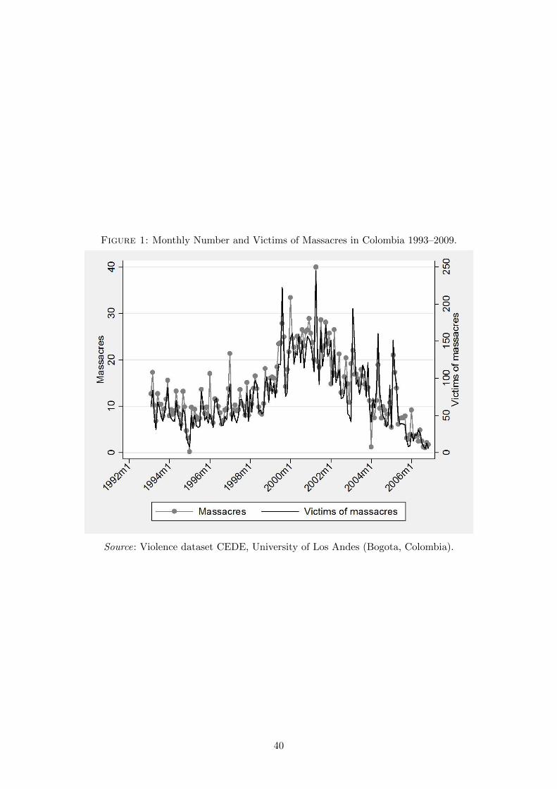
Figure 1: Monthly Number and Victims of Massacres in Colombia 1993–2009.

Source: Violence dataset CEDE, University of Los Andes (Bogota, Colombia).

40

Figure 2: Victims of Massacres in Colombia in 2000 and 2005.

19-73

10–18

HCB municipality

Other municipality

5–9

1–4

Source: Author‘s calculations.

41

Figure 3: Monthly Victims of Massacres by City.

Source: Violence dataset CEDE, University of Los Andes (Bogota, Colombia).

42

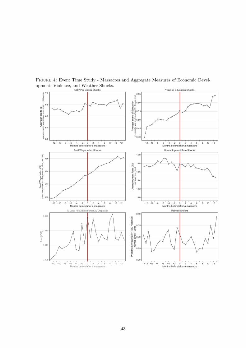
Figure 4: Event Time Study - Massacres and Aggregate Measures of Economic Devel-opment, Violence, and Weather Shocks.

6.2

6.4

6.6

6.8

7.0

−12 −10 −8 −6 −4 −2 0 2 4 6 8 10 12Months before/after a massacre

GDP Per Capita Shocks

GD

P pe

r cap

ita ($

) (y

ear–

mun

icip

ality

leve

l; M

illio

ns p

esos

, US

$1 ~

2,0

00 p

esos

)

6.40

6.45

6.50

6.55

6.65

6.60

−12 −10 −8 −6 −4 −2 0 2 4 6 8 10 12Months before/after a massacre

Years of Education Shocks

Ave

rage

Yea

rs o

f Edu

catio

n(m

unic

ipal

ity–y

ear l

evel

; As

of a

ge 3

0—C

ensu

s da

ta)

130

132

134

136

−12 −10 −8 −6 −4 −2 0 2 4 6 8 10 12Months before/after a massacre

Real Wage Index Shocks

Rea

l Wag

e In

dex

(%)

(199

0-20

06; m

onth

-yea

r lev

el; b

asel

ine:

100

%, J

an 1

990)

13.0

13.2

13.4

13.6

13.8

14.0

−12 −10 −8 −6 −4 −2 0 2 4 6 8 10 12Months before/after a massacre

Unemployment Rate Shocks

Une

mpl

oym

ent R

ate

(%)

(yea

r-de

partm

ent l

evel

)

0.005

0.010

0.015

0.020

−12 −10 −8 −6 −4 −2 0 2 4 6 8 10 12Months before/after a massacre

% Local Population Forcefully Displaced

Pro

b(ID

P)

0.20

0.25

0.30

0.35

0.40

−12 −10 −8 −6 −4 −2 0 2 4 6 8 10 12Months before/after a massacre

Rainfall Shocks

Prob

(Mon

thly

rain

fall

> 1S

D h

isto

rical

rain

fall

sinc

e 1980

)

43

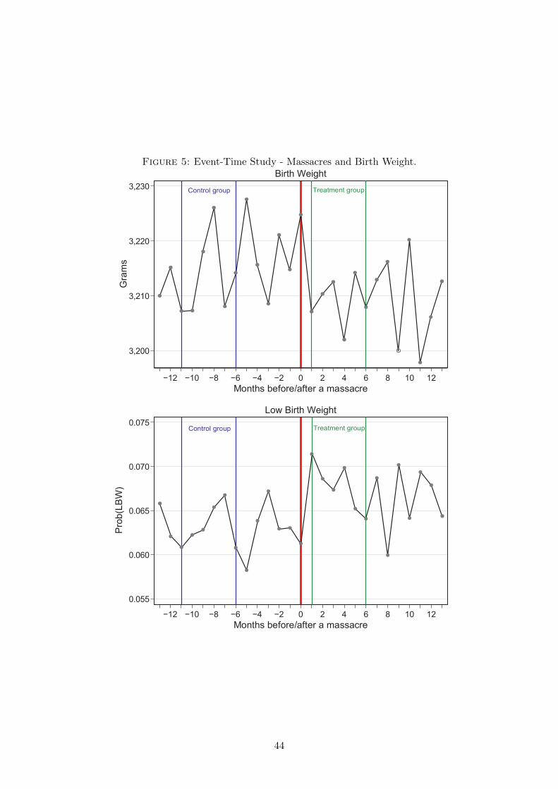
Figure 5: Event-Time Study - Massacres and Birth Weight.

3,210

3,220

3,230

3,200

−12 −10 −8 −6 −4 −2 0 2 4 6 8 10 12Months before/after a massacre

Birth Weight

Gra

ms

Control group Treatment group

0.055

0.060

0.065

0.070

0.075

−12 −10 −8 −6 −4 −2 0 2 4 6 8 10 12Months before/after a massacre

Low Birth Weight

Pro

b(LB

W)

Control group Treatment group

44

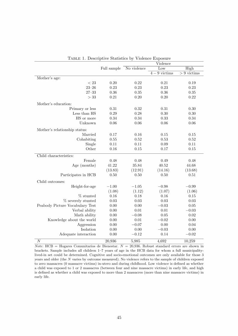
Table 1. Descriptive Statistics by Violence ExposureViolence

Full sample No violence Low High4 − 9 victims > 9 victims

Mother’s age:< 23 0.20 0.22 0.21 0.19

23–26 0.23 0.23 0.23 0.2327–33 0.36 0.35 0.36 0.35> 33 0.21 0.20 0.20 0.22

Mother’s education:Primary or less 0.31 0.32 0.31 0.30

Less than HS 0.29 0.28 0.30 0.30HS or more 0.34 0.34 0.33 0.34

Unknown 0.06 0.06 0.06 0.06

Mother’s relationship status:Married 0.17 0.16 0.15 0.15

Cohabiting 0.55 0.52 0.53 0.52Single 0.11 0.11 0.09 0.11Other 0.16 0.15 0.17 0.15

Child characteristics:Female 0.48 0.48 0.49 0.48

Age (months) 41.22 35.84 40.52 44.68(13.83) (12.91) (14.16) (13.68)

Participates in HCB 0.50 0.50 0.50 0.51

Child outcomes:Height-for-age −1.00 −1.05 −0.98 −0.99

(1.08) (1.12) (1.07) (1.06)% stunted 0.16 0.18 0.16 0.15

% severely stunted 0.03 0.03 0.03 0.03Peabody Picture Vocabulary Test 0.00 0.00 −0.03 0.05

Verbal ability 0.00 0.01 0.01 −0.03Math ability 0.00 −0.08 0.05 0.02

Knowledge about the world 0.00 0.01 −0.02 0.00Aggression 0.00 −0.07 0.00 0.04

Isolation 0.00 0.00 −0.03 0.00Adequate interaction 0.00 −0.12 0.14 −0.02

N 20,936 5,985 4,692 10,259Note: HCB = Hogares Comunitarios de Bienestar. N = 20,936. Robust standard errors are shown inbrackets. Sample includes all children 1–7 years of age in the HCB data for whom a full municipality-lived-in set could be determined. Cognitive and socio-emotional outcomes are only available for those 3years and older (the N varies by outcome measured). No violence refers to the sample of children exposedto zero massacres (0 massacre victims) in-utero and during childhood. Low violence is defined as whethera child was exposed to 1 or 2 massacres (between four and nine massacre victims) in early life, and highis defined as whether a child was exposed to more than 2 massacres (more than nine massacre victims) inearly life.

45

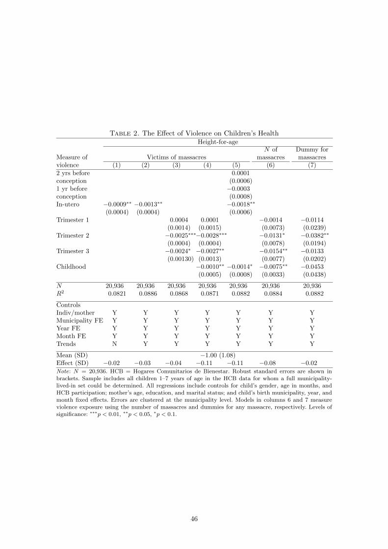
Table 2. The Effect of Violence on Children’s HealthHeight-for-age

Measure of Victims of massacresN of

massacresDummy formassacres

violence (1) (2) (3) (4) (5) (6) (7)2 yrs before 0.0001conception (0.0006)1 yr before −0.0003conception (0.0008)In-utero −0.0009∗∗ −0.0013∗∗ −0.0018∗∗

(0.0004) (0.0004) (0.0006)Trimester 1 0.0004 0.0001 −0.0014 −0.0114

(0.0014) (0.0015) (0.0073) (0.0239)Trimester 2 −0.0025∗∗∗−0.0028∗∗∗ −0.0131∗ −0.0382∗∗

(0.0004) (0.0004) (0.0078) (0.0194)Trimester 3 −0.0024∗ −0.0027∗∗ −0.0154∗∗ −0.0133

(0.00130) (0.0013) (0.0077) (0.0202)Childhood −0.0010∗∗ −0.0014∗ −0.0075∗∗ −0.0453

(0.0005) (0.0008) (0.0033) (0.0438)

N 20,936 20,936 20,936 20,936 20,936 20,936 20,936R2 0.0821 0.0886 0.0868 0.0871 0.0882 0.0884 0.0882

ControlsIndiv/mother Y Y Y Y Y Y YMunicipality FE Y Y Y Y Y Y YYear FE Y Y Y Y Y Y YMonth FE Y Y Y Y Y Y YTrends N Y Y Y Y Y Y

Mean (SD) −1.00 (1.08)Effect (SD) −0.02 −0.03 −0.04 −0.11 −0.11 −0.08 −0.02Note: N = 20,936. HCB = Hogares Comunitarios de Bienestar. Robust standard errors are shown inbrackets. Sample includes all children 1–7 years of age in the HCB data for whom a full municipality-lived-in set could be determined. All regressions include controls for child’s gender, age in months, andHCB participation; mother’s age, education, and marital status; and child’s birth municipality, year, andmonth fixed effects. Errors are clustered at the municipality level. Models in columns 6 and 7 measureviolence exposure using the number of massacres and dummies for any massacre, respectively. Levels ofsignificance: ∗∗∗p < 0.01, ∗∗p < 0.05, ∗p < 0.1.

46

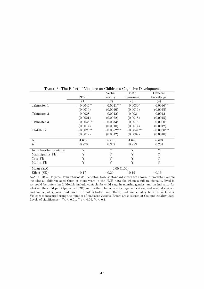
Table 3. The Effect of Violence on Children’s Cognitive Development

PPVTVerbalability

Mathreasoning

Generalknowledge

(1) (2) (3) (4)Trimester 1 −0.0046∗∗ −0.0041∗∗∗ −0.0030∗ −0.0036∗∗

(0.0019) (0.0010) (0.0016) (0.0015)Trimester 2 −0.0028 −0.0042∗ −0.002 −0.0012

(0.0021) (0.0022) (0.0018) (0.0015)Trimester 3 −0.0038∗∗∗ −0.0033∗ −0.0014 −0.0020∗

(0.0014) (0.0018) (0.0014) (0.0012)Childhood −0.0025∗∗ −0.0052∗∗∗ −0.0044∗∗∗ −0.0030∗∗∗

(0.0012) (0.0012) (0.0009) (0.0010)

N 4,669 4,711 4,648 4,703R2 0.270 0.332 0.253 0.201

Indiv/mother controls Y Y Y YMunicipality FE Y Y Y YYear FE Y Y Y YMonth FE Y Y Y Y

Mean (SD) 0.00 (1.00)Effect (SD) −0.17 −0.29 −0.19 −0.16

Note: HCB = Hogares Comunitarios de Bienestar. Robust standard errors are shown in brackets. Sampleincludes all children aged three or more years in the HCB data for whom a full municipality-lived-inset could be determined. Models include controls for child (age in months, gender, and an indicator forwhether the child participates in HCB) and mother characteristics (age, education, and marital status);and municipality, year, and month of child’s birth fixed effects, and municipality linear time trends.Violence is measured using the number of massacre victims. Errors are clustered at the municipality level.Levels of significance: ∗∗∗p < 0.01, ∗∗p < 0.05, ∗p < 0.1.

47

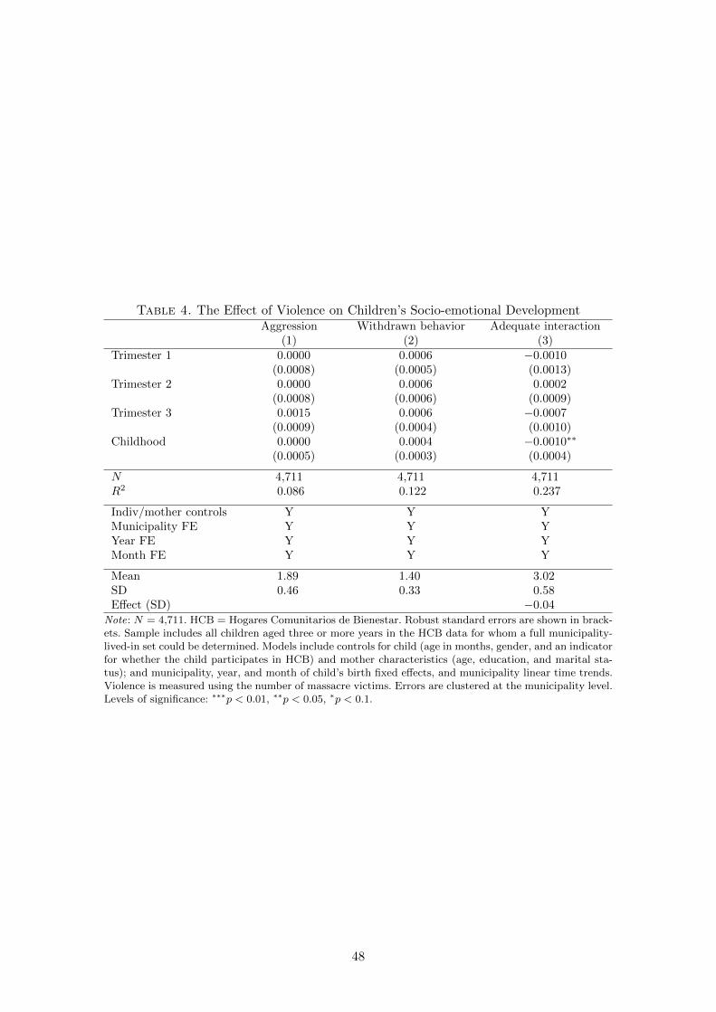
Table 4. The Effect of Violence on Children’s Socio-emotional DevelopmentAggression Withdrawn behavior Adequate interaction

(1) (2) (3)Trimester 1 0.0000 0.0006 −0.0010

(0.0008) (0.0005) (0.0013)Trimester 2 0.0000 0.0006 0.0002

(0.0008) (0.0006) (0.0009)Trimester 3 0.0015 0.0006 −0.0007

(0.0009) (0.0004) (0.0010)Childhood 0.0000 0.0004 −0.0010∗∗

(0.0005) (0.0003) (0.0004)

N 4,711 4,711 4,711R2 0.086 0.122 0.237

Indiv/mother controls Y Y YMunicipality FE Y Y YYear FE Y Y YMonth FE Y Y Y

Mean 1.89 1.40 3.02SD 0.46 0.33 0.58Effect (SD) −0.04

Note: N = 4,711. HCB = Hogares Comunitarios de Bienestar. Robust standard errors are shown in brack-ets. Sample includes all children aged three or more years in the HCB data for whom a full municipality-lived-in set could be determined. Models include controls for child (age in months, gender, and an indicatorfor whether the child participates in HCB) and mother characteristics (age, education, and marital sta-tus); and municipality, year, and month of child’s birth fixed effects, and municipality linear time trends.Violence is measured using the number of massacre victims. Errors are clustered at the municipality level.Levels of significance: ∗∗∗p < 0.01, ∗∗p < 0.05, ∗p < 0.1.

48

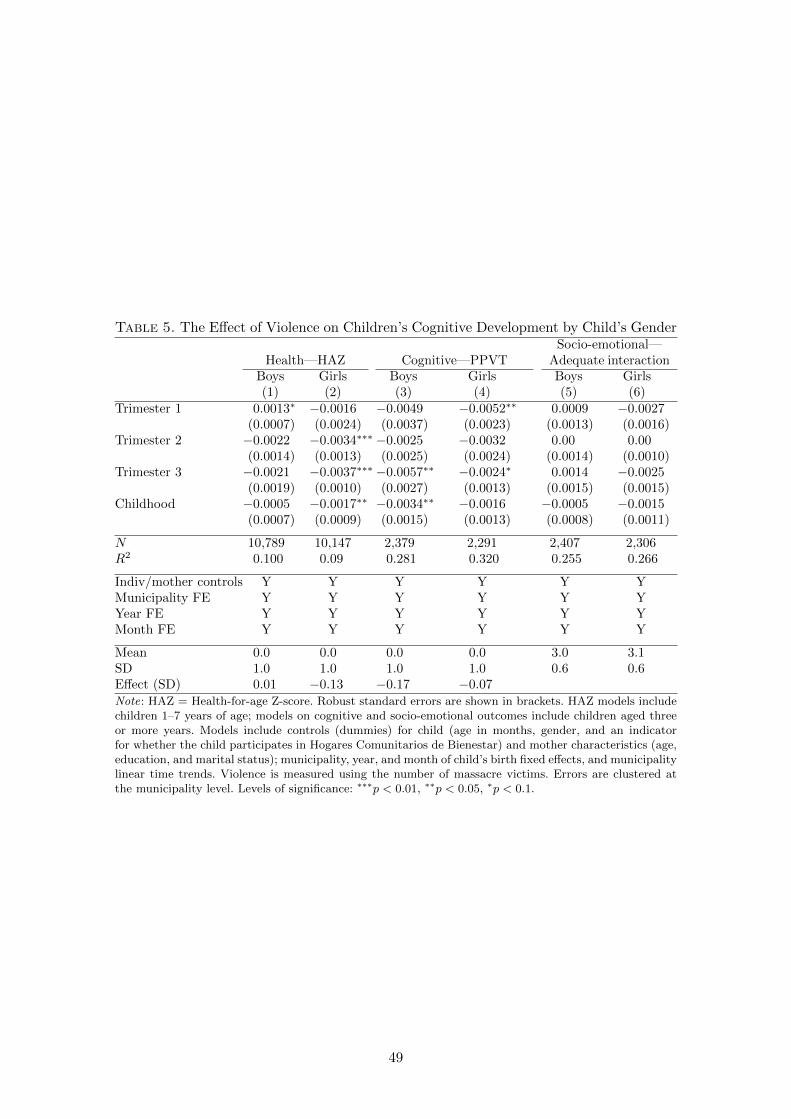
Table 5. The Effect of Violence on Children’s Cognitive Development by Child’s Gender

Health—HAZ Cognitive—PPVTSocio-emotional—

Adequate interactionBoys Girls Boys Girls Boys Girls(1) (2) (3) (4) (5) (6)

Trimester 1 0.0013∗ −0.0016 −0.0049 −0.0052∗∗ 0.0009 −0.0027(0.0007) (0.0024) (0.0037) (0.0023) (0.0013) (0.0016)

Trimester 2 −0.0022 −0.0034∗∗∗ −0.0025 −0.0032 0.00 0.00(0.0014) (0.0013) (0.0025) (0.0024) (0.0014) (0.0010)

Trimester 3 −0.0021 −0.0037∗∗∗ −0.0057∗∗ −0.0024∗ 0.0014 −0.0025(0.0019) (0.0010) (0.0027) (0.0013) (0.0015) (0.0015)

Childhood −0.0005 −0.0017∗∗ −0.0034∗∗ −0.0016 −0.0005 −0.0015(0.0007) (0.0009) (0.0015) (0.0013) (0.0008) (0.0011)

N 10,789 10,147 2,379 2,291 2,407 2,306R2 0.100 0.09 0.281 0.320 0.255 0.266

Indiv/mother controls Y Y Y Y Y YMunicipality FE Y Y Y Y Y YYear FE Y Y Y Y Y YMonth FE Y Y Y Y Y Y

Mean 0.0 0.0 0.0 0.0 3.0 3.1SD 1.0 1.0 1.0 1.0 0.6 0.6Effect (SD) 0.01 −0.13 −0.17 −0.07Note: HAZ = Health-for-age Z-score. Robust standard errors are shown in brackets. HAZ models includechildren 1–7 years of age; models on cognitive and socio-emotional outcomes include children aged threeor more years. Models include controls (dummies) for child (age in months, gender, and an indicatorfor whether the child participates in Hogares Comunitarios de Bienestar) and mother characteristics (age,education, and marital status); municipality, year, and month of child’s birth fixed effects, and municipalitylinear time trends. Violence is measured using the number of massacre victims. Errors are clustered atthe municipality level. Levels of significance: ∗∗∗p < 0.01, ∗∗p < 0.05, ∗p < 0.1.

49

Table 6. The Effect of Violence on Children’s Development by Mother’s Education

Health—HAZ Cognitive—PPVTSocio-emotional—

Adequate interactionLow High Low High Low High

Trimester 1 −0.0002 −0.0003 −0.0062∗∗ −0.0017 −0.0020 −0.0003( 0.0021) ( 0.0011) ( 0.0024) ( 0.0015) ( 0.0012) ( 0.0012)

Trimester 2 −0.0014∗ −0.0036∗∗∗ −0.0035 −0.0004 −0.0008 0.0000( 0.0008) ( 0.0012) ( 0.0039) ( 0.0024) ( 0.0010) ( 0.0015)

Trimester 3 −0.0028∗ −0.0032∗∗ −0.0038∗∗ −0.0027 −0.0009 −0.0014( 0.0015) ( 0.0016) ( 0.0014) ( 0.0035) ( 0.0013) ( 0.0012)

Childhood −0.0014 −0.0005 −0.0038∗∗ 0.0003 −0.0014∗ −0.0011( 0.0012) ( 0.0009) ( 0.0018) ( 0.0021) ( 0.0001) ( 0.0008)

N 10,347 9,362 2,405 1,954 2,439 1,960R2 0.0780 0.0890 0.2750 0.2720 0.2600 0.2500

Indiv/mother controls Y Y Y Y Y YMunicipality FE Y Y Y Y Y YYear FE Y Y Y Y Y YMonth FE Y Y Y Y Y Y

Mean −0.9000 −1.2000 −0.2000 0.1000 3.0000 3.1000SD 1.0000 1.0000 0.9000 1.0000 0.6000 0.6000Effect (SD) −0.0400 −0.0600 −0.2300 −0.0500Note: HAZ = Health-for-age Z-score. Robust standard errors are shown in brackets. HAZ models includechildren 1–7 years of age; models on cognitive and socio-emotional outcomes include children aged threeor more years. Models include controls (dummies) for child (age in months, gender, and an indicatorfor whether the child participates in Hogares Comunitarios de Bienestar) and mother characteristics (age,education, and marital status); municipality, year, and month of child’s birth fixed effects, and municipalitylinear time trends. Violence is measured using the number of massacre victims. Errors are clustered atthe municipality level. Levels of significance: ∗∗∗p < 0.01, ∗∗p < 0.05, ∗p < 0.1.

50

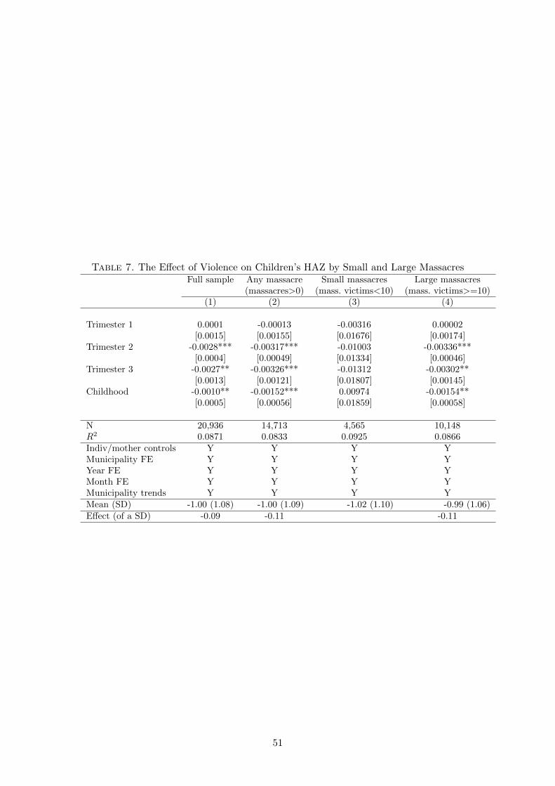
Table 7. The Effect of Violence on Children’s HAZ by Small and Large MassacresFull sample Any massacre Small massacres Large massacres

(massacres>0) (mass. victims<10) (mass. victims>=10)(1) (2) (3) (4)

Trimester 1 0.0001 -0.00013 -0.00316 0.00002[0.0015] [0.00155] [0.01676] [0.00174]

Trimester 2 -0.0028*** -0.00317*** -0.01003 -0.00336***[0.0004] [0.00049] [0.01334] [0.00046]

Trimester 3 -0.0027** -0.00326*** -0.01312 -0.00302**[0.0013] [0.00121] [0.01807] [0.00145]

Childhood -0.0010** -0.00152*** 0.00974 -0.00154**[0.0005] [0.00056] [0.01859] [0.00058]

N 20,936 14,713 4,565 10,148R2 0.0871 0.0833 0.0925 0.0866Indiv/mother controls Y Y Y YMunicipality FE Y Y Y YYear FE Y Y Y YMonth FE Y Y Y YMunicipality trends Y Y Y YMean (SD) -1.00 (1.08) -1.00 (1.09) -1.02 (1.10) -0.99 (1.06)Effect (of a SD) -0.09 -0.11 -0.11

51

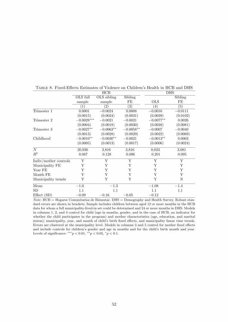
Table 8. Fixed-Effects Estimates of Violence on Children’s Health in HCB and DHSHCB DHS

OLS fullsample

OLS siblingsample

SiblingFE OLS

SiblingFE

(1) (2) (3) (4) (5)Trimester 1 0.0001 −0.0024 0.0008 −0.0016 −0.0111

(0.0015) (0.0024) (0.0031) (0.0039) (0.0102)Trimester 2 −0.0028∗∗∗ −0.0021 −0.0021 −0.0077∗∗ 0.0026

(0.0004) (0.0018) (0.0030) (0.0038) (0.0081)Trimester 3 −0.0027∗∗ −0.0063∗∗ −0.0058∗∗ −0.0007 −0.0040

(0.0013) (0.0028) (0.0029) (0.0022) (0.0069)Childhood −0.0010∗∗ −0.0030∗∗ −0.0021 −0.0013∗∗ 0.0003

(0.0005) (0.0013) (0.0017) (0.0006) (0.0024)

N 20,936 3,816 3,816 8,023 3,081R2 0.087 0.128 0.096 0.201 0.095

Indiv/mother controls Y Y Y Y YMunicipality FE Y Y Y Y YYear FE Y Y Y Y YMonth FE Y Y Y Y YMunicipality trends Y Y Y Y N

Mean −1.0 −1.3 −1.08 −1.4SD 1.1 1.1 1.1 1.1Effect (SD) −0.09 −0.16 −0.05 −0.12Note: HCB = Hogares Comunitarios de Bienestar. DHS = Demography and Health Survey. Robust stan-dard errors are shown in brackets. Sample includes children between aged 12 or more months in the HCBdata for whom a full municipality-lived-in set could be determined and 24 or more months in DHS. Modelsin columns 1, 2, and 4 control for child (age in months, gender, and in the case of HCB, an indicator forwhether the child participates in the program) and mother characteristics (age, education, and maritalstatus); municipality, year, and month of child’s birth fixed effects, and municipality linear time trends.Errors are clustered at the municipality level. Models in columns 3 and 5 control for mother fixed effectsand include controls for children’s gender and age in months and for the child’s birth month and year.Levels of significance: ∗∗∗p < 0.01, ∗∗p < 0.05, ∗p < 0.1.

52

Table 9. Fixed-Effects Estimates of Violence on Children’s Cognitive Development inHCB and ELCA

PPVT ELCAOLS fullsample

OLS siblingsample

SiblingFE OLS

SiblingFE

(1) (2) (3) (4) (5)Trimester 1 −0.0045∗∗ −0.0043∗ −0.0096 −0.0184∗∗ −0.0585∗∗

(0.0018) (0.0025) (0.0091) (0.0088) (0.0249)Trimester 2 −0.0024 −0.0043 −0.0119 −0.0062 −0.0318

(0.0021) (0.0042) (0.0123) (0.0065) (0.0247)Trimester 3 −0.0034∗ −0.0031 −0.0237∗∗ 0.0049 −0.0101

(0.0018) (0.0030) (0.0094) (0.0094) (0.0286)Childhood −0.0021∗ −0.0006 −0.0009 0.0115 0.0232

(0.0012) (0.0025) (0.0056) (0.0313) (0.0183)

N 4,669 740 740 1,099 887R2 0.274 0.38 0.52 0.36101 0.349

Indiv/mother or HH controls Y Y Y Y YMunicipality FE Y Y Y Y YYear FE Y Y Y Y YMonth FE Y Y Y Y YMunicipality trends Y Y Y Y N

Mean 0.0 −0.3 0.0SD 1.0 1.0 1.0Effect (SD) −0.15 −0.04 −0.21 −0.17 −0.53Note: ELCA = Colombian Longitudinal Survey conducted by Universidad de los Andes. Robust standarderrors are shown in brackets. Sample includes children aged 36 or more months in the Hogares Comunitariosde Bienestar data for whom a full municipality-lived-in set could be determined. Models in columns 1 and2 control for child (age in months, gender, and an indicator for whether the child participates in theprogram) and mother characteristics (age, education, and marital status); municipality, year, and monthof child’s birth fixed effects, and municipality linear time trends. Errors are clustered at the municipalitylevel. Model in column 3 controls for mother fixed effects and include controls for child’s gender and agein months and fixed effects for the child’s birth month and year. . Levels of significance: ∗∗∗p < 0.01,∗∗p < 0.05, ∗p < 0.1.

53

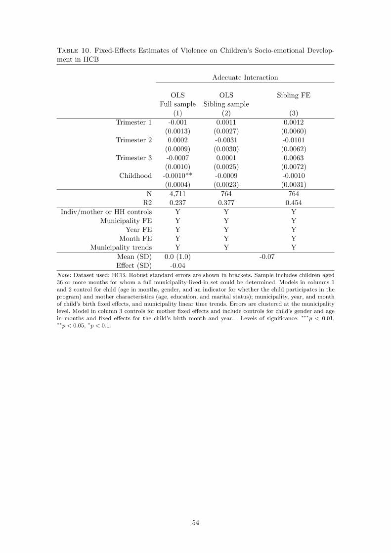
Table 10. Fixed-Effects Estimates of Violence on Children’s Socio-emotional Develop-ment in HCB

Adecuate Interaction

OLS OLS Sibling FEFull sample Sibling sample

(1) (2) (3)

Trimester 1 -0.001 0.0011 0.0012(0.0013) (0.0027) (0.0060)

Trimester 2 0.0002 -0.0031 -0.0101(0.0009) (0.0030) (0.0062)

Trimester 3 -0.0007 0.0001 0.0063(0.0010) (0.0025) (0.0072)

Childhood -0.0010** -0.0009 -0.0010(0.0004) (0.0023) (0.0031)

N 4,711 764 764R2 0.237 0.377 0.454

Indiv/mother or HH controls Y Y YMunicipality FE Y Y Y

Year FE Y Y YMonth FE Y Y Y

Municipality trends Y Y Y

Mean (SD) 0.0 (1.0) -0.07Effect (SD) -0.04

Note: Dataset used: HCB. Robust standard errors are shown in brackets. Sample includes children aged36 or more months for whom a full municipality-lived-in set could be determined. Models in columns 1and 2 control for child (age in months, gender, and an indicator for whether the child participates in theprogram) and mother characteristics (age, education, and marital status); municipality, year, and monthof child’s birth fixed effects, and municipality linear time trends. Errors are clustered at the municipalitylevel. Model in column 3 controls for mother fixed effects and include controls for child’s gender and agein months and fixed effects for the child’s birth month and year. . Levels of significance: ∗∗∗p < 0.01,∗∗p < 0.05, ∗p < 0.1.

54

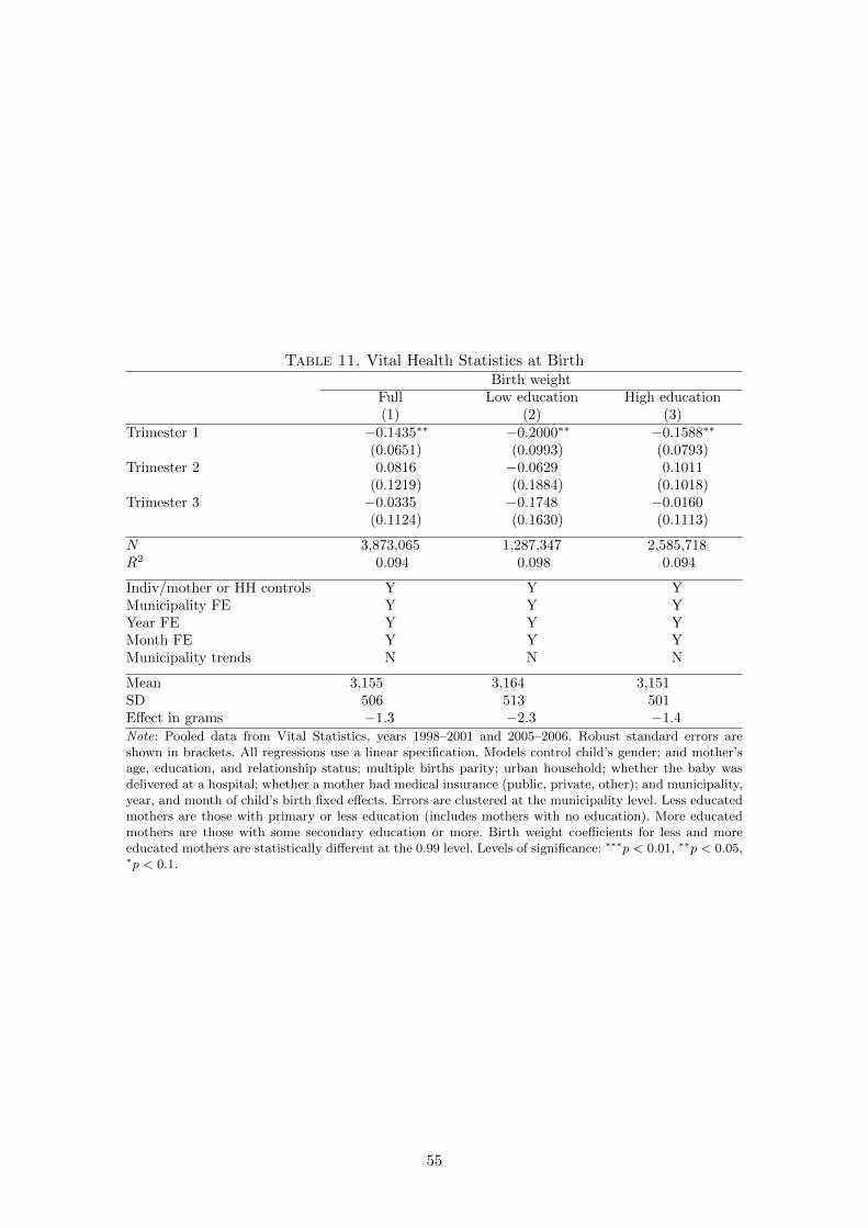
Table 11. Vital Health Statistics at BirthBirth weight

Full Low education High education(1) (2) (3)

Trimester 1 −0.1435∗∗ −0.2000∗∗ −0.1588∗∗

(0.0651) (0.0993) (0.0793)Trimester 2 0.0816 −0.0629 0.1011

(0.1219) (0.1884) (0.1018)Trimester 3 −0.0335 −0.1748 −0.0160

(0.1124) (0.1630) (0.1113)

N 3,873,065 1,287,347 2,585,718R2 0.094 0.098 0.094

Indiv/mother or HH controls Y Y YMunicipality FE Y Y YYear FE Y Y YMonth FE Y Y YMunicipality trends N N N

Mean 3,155 3,164 3,151SD 506 513 501Effect in grams −1.3 −2.3 −1.4Note: Pooled data from Vital Statistics, years 1998–2001 and 2005–2006. Robust standard errors areshown in brackets. All regressions use a linear specification. Models control child’s gender; and mother’sage, education, and relationship status; multiple births parity; urban household; whether the baby wasdelivered at a hospital; whether a mother had medical insurance (public, private, other); and municipality,year, and month of child’s birth fixed effects. Errors are clustered at the municipality level. Less educatedmothers are those with primary or less education (includes mothers with no education). More educatedmothers are those with some secondary education or more. Birth weight coefficients for less and moreeducated mothers are statistically different at the 0.99 level. Levels of significance: ∗∗∗p < 0.01, ∗∗p < 0.05,∗p < 0.1.

55

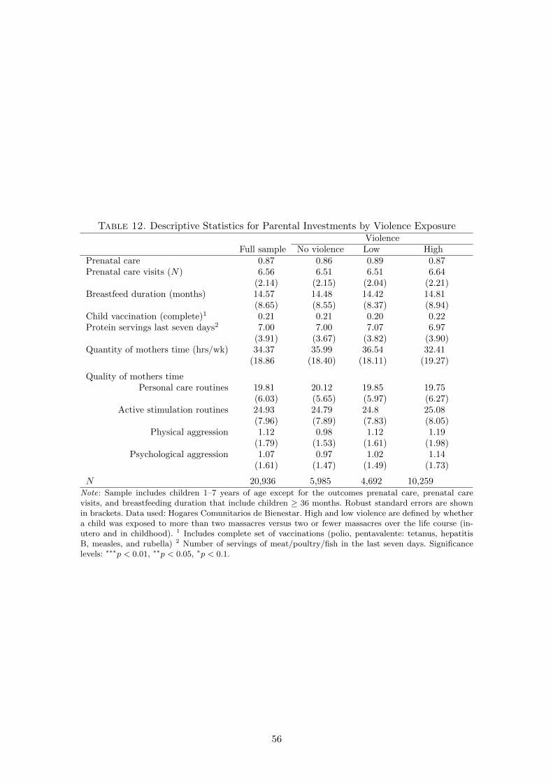
Table 12. Descriptive Statistics for Parental Investments by Violence ExposureViolence

Full sample No violence Low HighPrenatal care 0.87 0.86 0.89 0.87Prenatal care visits (N) 6.56 6.51 6.51 6.64

(2.14) (2.15) (2.04) (2.21)Breastfeed duration (months) 14.57 14.48 14.42 14.81

(8.65) (8.55) (8.37) (8.94)Child vaccination (complete)1 0.21 0.21 0.20 0.22Protein servings last seven days2 7.00 7.00 7.07 6.97

(3.91) (3.67) (3.82) (3.90)Quantity of mothers time (hrs/wk) 34.37 35.99 36.54 32.41

(18.86 (18.40) (18.11) (19.27)

Quality of mothers timePersonal care routines 19.81 20.12 19.85 19.75

(6.03) (5.65) (5.97) (6.27)Active stimulation routines 24.93 24.79 24.8 25.08

(7.96) (7.89) (7.83) (8.05)Physical aggression 1.12 0.98 1.12 1.19

(1.79) (1.53) (1.61) (1.98)Psychological aggression 1.07 0.97 1.02 1.14

(1.61) (1.47) (1.49) (1.73)

N 20,936 5,985 4,692 10,259Note: Sample includes children 1–7 years of age except for the outcomes prenatal care, prenatal carevisits, and breastfeeding duration that include children ≥ 36 months. Robust standard errors are shownin brackets. Data used: Hogares Comunitarios de Bienestar. High and low violence are defined by whethera child was exposed to more than two massacres versus two or fewer massacres over the life course (in-utero and in childhood). 1 Includes complete set of vaccinations (polio, pentavalente: tetanus, hepatitisB, measles, and rubella) 2 Number of servings of meat/poultry/fish in the last seven days. Significancelevels: ∗∗∗p < 0.01, ∗∗p < 0.05, ∗p < 0.1.

56

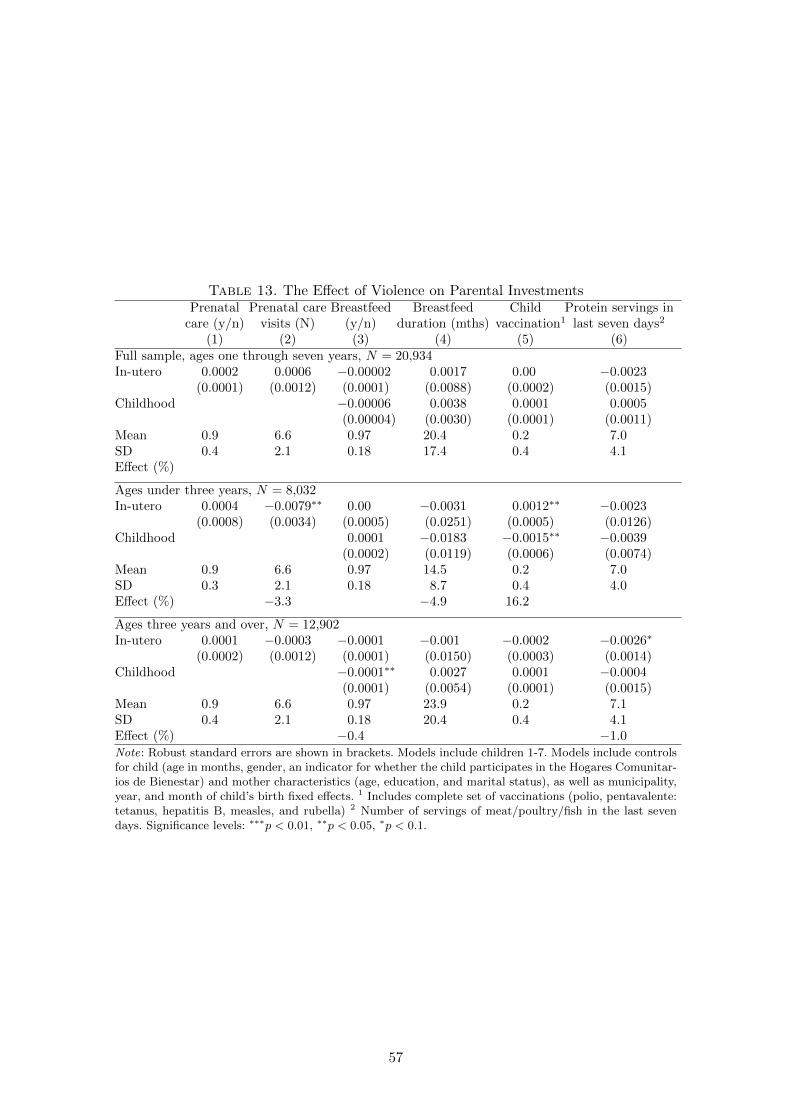
Table 13. The Effect of Violence on Parental InvestmentsPrenatal

care (y/n)Prenatal care

visits (N)Breastfeed

(y/n)Breastfeed

duration (mths)Child

vaccination1Protein servings in

last seven days2

(1) (2) (3) (4) (5) (6)Full sample, ages one through seven years, N = 20,934In-utero 0.0002 0.0006 −0.00002 0.0017 0.00 −0.0023

(0.0001) (0.0012) (0.0001) (0.0088) (0.0002) (0.0015)Childhood −0.00006 0.0038 0.0001 0.0005

(0.00004) (0.0030) (0.0001) (0.0011)Mean 0.9 6.6 0.97 20.4 0.2 7.0SD 0.4 2.1 0.18 17.4 0.4 4.1Effect (%)

Ages under three years, N = 8,032In-utero 0.0004 −0.0079∗∗ 0.00 −0.0031 0.0012∗∗ −0.0023

(0.0008) (0.0034) (0.0005) (0.0251) (0.0005) (0.0126)Childhood 0.0001 −0.0183 −0.0015∗∗ −0.0039

(0.0002) (0.0119) (0.0006) (0.0074)Mean 0.9 6.6 0.97 14.5 0.2 7.0SD 0.3 2.1 0.18 8.7 0.4 4.0Effect (%) −3.3 −4.9 16.2

Ages three years and over, N = 12,902In-utero 0.0001 −0.0003 −0.0001 −0.001 −0.0002 −0.0026∗

(0.0002) (0.0012) (0.0001) (0.0150) (0.0003) (0.0014)Childhood −0.0001∗∗ 0.0027 0.0001 −0.0004

(0.0001) (0.0054) (0.0001) (0.0015)Mean 0.9 6.6 0.97 23.9 0.2 7.1SD 0.4 2.1 0.18 20.4 0.4 4.1Effect (%) −0.4 −1.0Note: Robust standard errors are shown in brackets. Models include children 1-7. Models include controlsfor child (age in months, gender, an indicator for whether the child participates in the Hogares Comunitar-ios de Bienestar) and mother characteristics (age, education, and marital status), as well as municipality,year, and month of child’s birth fixed effects. 1 Includes complete set of vaccinations (polio, pentavalente:tetanus, hepatitis B, measles, and rubella) 2 Number of servings of meat/poultry/fish in the last sevendays. Significance levels: ∗∗∗p < 0.01, ∗∗p < 0.05, ∗p < 0.1.

57

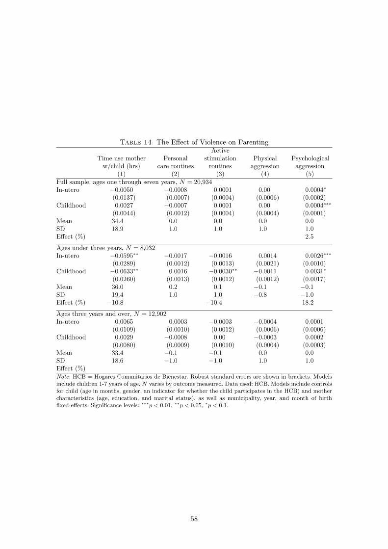
Table 14. The Effect of Violence on Parenting

Time use motherw/child (hrs)

Personalcare routines

Activestimulation

routinesPhysical

aggressionPsychological

aggression(1) (2) (3) (4) (5)

Full sample, ages one through seven years, N = 20,934In-utero −0.0050 −0.0008 0.0001 0.00 0.0004∗

(0.0137) (0.0007) (0.0004) (0.0006) (0.0002)Childhood 0.0027 −0.0007 0.0001 0.00 0.0004∗∗∗

(0.0044) (0.0012) (0.0004) (0.0004) (0.0001)Mean 34.4 0.0 0.0 0.0 0.0SD 18.9 1.0 1.0 1.0 1.0Effect (%) 2.5

Ages under three years, N = 8,032In-utero −0.0595∗∗ −0.0017 −0.0016 0.0014 0.0026∗∗∗

(0.0289) (0.0012) (0.0013) (0.0021) (0.0010)Childhood −0.0633∗∗ 0.0016 −0.0030∗∗ −0.0011 0.0031∗

(0.0260) (0.0013) (0.0012) (0.0012) (0.0017)Mean 36.0 0.2 0.1 −0.1 −0.1SD 19.4 1.0 1.0 −0.8 −1.0Effect (%) −10.8 −10.4 18.2

Ages three years and over, N = 12,902In-utero 0.0065 0.0003 −0.0003 −0.0004 0.0001

(0.0109) (0.0010) (0.0012) (0.0006) (0.0006)Childhood 0.0029 −0.0008 0.00 −0.0003 0.0002

(0.0080) (0.0009) (0.0010) (0.0004) (0.0003)Mean 33.4 −0.1 −0.1 0.0 0.0SD 18.6 −1.0 −1.0 1.0 1.0Effect (%)Note: HCB = Hogares Comunitarios de Bienestar. Robust standard errors are shown in brackets. Modelsinclude children 1-7 years of age. N varies by outcome measured. Data used: HCB. Models include controlsfor child (age in months, gender, an indicator for whether the child participates in the HCB) and mothercharacteristics (age, education, and marital status), as well as municipality, year, and month of birthfixed-effects. Significance levels: ∗∗∗p < 0.01, ∗∗p < 0.05, ∗p < 0.1.

58

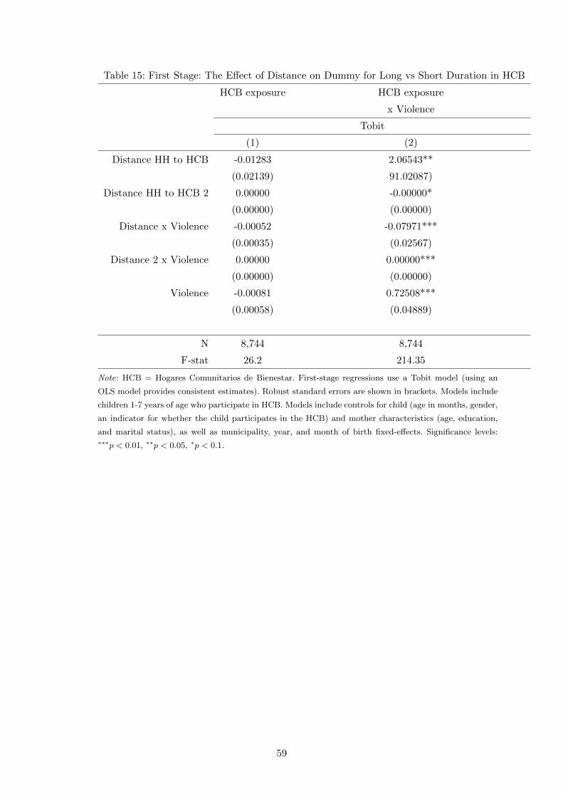
Table 15: First Stage: The Effect of Distance on Dummy for Long vs Short Duration in HCB

HCB exposure HCB exposure

x Violence

Tobit

(1) (2)

Distance HH to HCB -0.01283 2.06543**

(0.02139) 91.02087)

Distance HH to HCB 2 0.00000 -0.00000*

(0.00000) (0.00000)

Distance x Violence -0.00052 -0.07971***

(0.00035) (0.02567)

Distance 2 x Violence 0.00000 0.00000***

(0.00000) (0.00000)

Violence -0.00081 0.72508***

(0.00058) (0.04889)

N 8,744 8,744

F-stat 26.2 214.35

Note: HCB = Hogares Comunitarios de Bienestar. First-stage regressions use a Tobit model (using an

OLS model provides consistent estimates). Robust standard errors are shown in brackets. Models include

children 1-7 years of age who participate in HCB. Models include controls for child (age in months, gender,

an indicator for whether the child participates in the HCB) and mother characteristics (age, education,

and marital status), as well as municipality, year, and month of birth fixed-effects. Significance levels:∗∗∗p < 0.01, ∗∗p < 0.05, ∗p < 0.1.

59

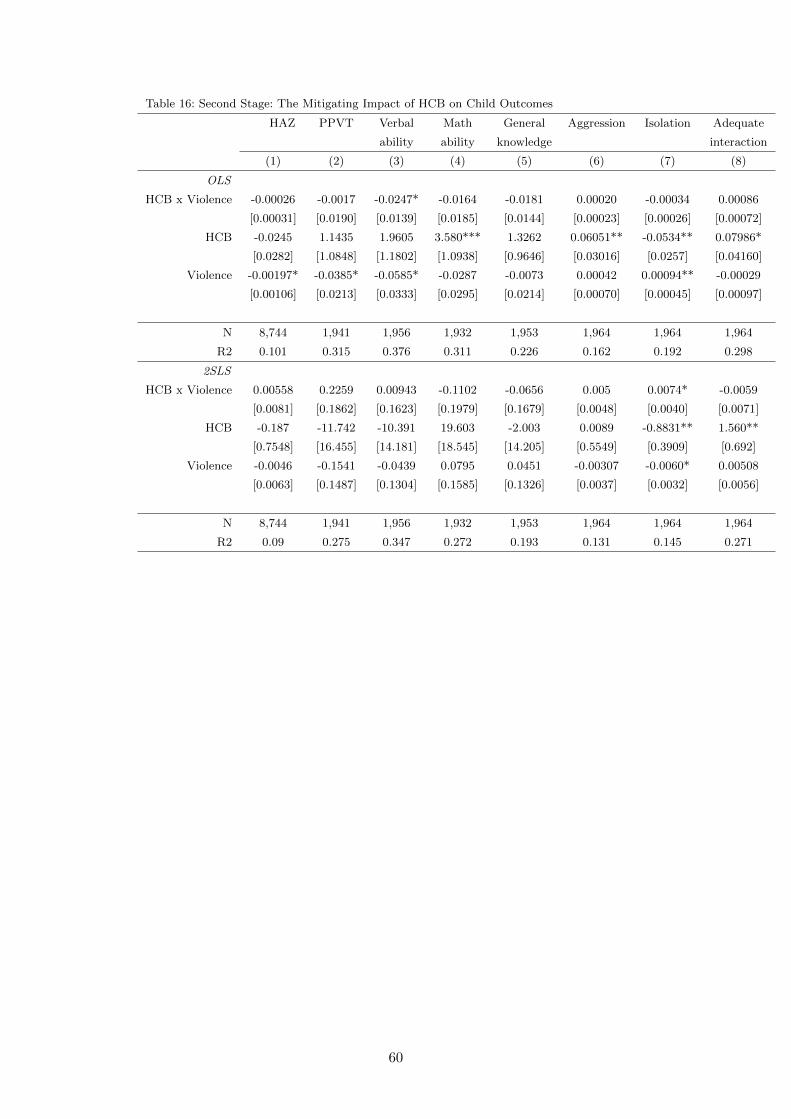
Table 16: Second Stage: The Mitigating Impact of HCB on Child Outcomes

HAZ PPVT Verbal Math General Aggression Isolation Adequate

ability ability knowledge interaction

(1) (2) (3) (4) (5) (6) (7) (8)

OLS

HCB x Violence -0.00026 -0.0017 -0.0247* -0.0164 -0.0181 0.00020 -0.00034 0.00086

[0.00031] [0.0190] [0.0139] [0.0185] [0.0144] [0.00023] [0.00026] [0.00072]

HCB -0.0245 1.1435 1.9605 3.580*** 1.3262 0.06051** -0.0534** 0.07986*

[0.0282] [1.0848] [1.1802] [1.0938] [0.9646] [0.03016] [0.0257] [0.04160]

Violence -0.00197* -0.0385* -0.0585* -0.0287 -0.0073 0.00042 0.00094** -0.00029

[0.00106] [0.0213] [0.0333] [0.0295] [0.0214] [0.00070] [0.00045] [0.00097]

N 8,744 1,941 1,956 1,932 1,953 1,964 1,964 1,964

R2 0.101 0.315 0.376 0.311 0.226 0.162 0.192 0.298

2SLS

HCB x Violence 0.00558 0.2259 0.00943 -0.1102 -0.0656 0.005 0.0074* -0.0059

[0.0081] [0.1862] [0.1623] [0.1979] [0.1679] [0.0048] [0.0040] [0.0071]

HCB -0.187 -11.742 -10.391 19.603 -2.003 0.0089 -0.8831** 1.560**

[0.7548] [16.455] [14.181] [18.545] [14.205] [0.5549] [0.3909] [0.692]

Violence -0.0046 -0.1541 -0.0439 0.0795 0.0451 -0.00307 -0.0060* 0.00508

[0.0063] [0.1487] [0.1304] [0.1585] [0.1326] [0.0037] [0.0032] [0.0056]

N 8,744 1,941 1,956 1,932 1,953 1,964 1,964 1,964

R2 0.09 0.275 0.347 0.272 0.193 0.131 0.145 0.271

60

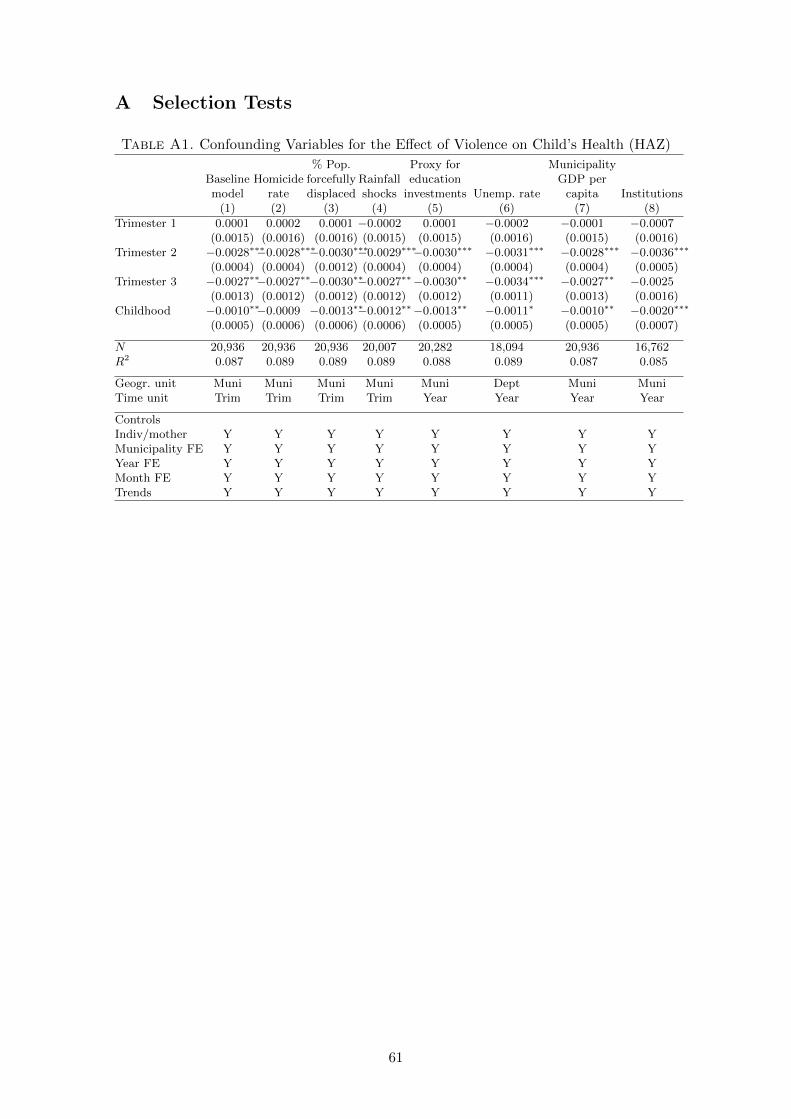
A Selection Tests

Table A1. Confounding Variables for the Effect of Violence on Child’s Health (HAZ)

Baselinemodel

Homiciderate

% Pop.forcefullydisplaced

Rainfallshocks

Proxy foreducation

investments Unemp. rate

MunicipalityGDP per

capita Institutions(1) (2) (3) (4) (5) (6) (7) (8)

Trimester 1 0.0001 0.0002 0.0001 −0.0002 0.0001 −0.0002 −0.0001 −0.0007(0.0015) (0.0016) (0.0016) (0.0015) (0.0015) (0.0016) (0.0015) (0.0016)

Trimester 2 −0.0028∗∗∗−0.0028∗∗∗−0.0030∗∗∗−0.0029∗∗∗−0.0030∗∗∗ −0.0031∗∗∗ −0.0028∗∗∗ −0.0036∗∗∗

(0.0004) (0.0004) (0.0012) (0.0004) (0.0004) (0.0004) (0.0004) (0.0005)Trimester 3 −0.0027∗∗−0.0027∗∗−0.0030∗∗−0.0027∗∗−0.0030∗∗ −0.0034∗∗∗ −0.0027∗∗ −0.0025

(0.0013) (0.0012) (0.0012) (0.0012) (0.0012) (0.0011) (0.0013) (0.0016)Childhood −0.0010∗∗−0.0009 −0.0013∗∗−0.0012∗∗−0.0013∗∗ −0.0011∗ −0.0010∗∗ −0.0020∗∗∗

(0.0005) (0.0006) (0.0006) (0.0006) (0.0005) (0.0005) (0.0005) (0.0007)

N 20,936 20,936 20,936 20,007 20,282 18,094 20,936 16,762R2 0.087 0.089 0.089 0.089 0.088 0.089 0.087 0.085

Geogr. unit Muni Muni Muni Muni Muni Dept Muni MuniTime unit Trim Trim Trim Trim Year Year Year Year

ControlsIndiv/mother Y Y Y Y Y Y Y YMunicipality FE Y Y Y Y Y Y Y YYear FE Y Y Y Y Y Y Y YMonth FE Y Y Y Y Y Y Y YTrends Y Y Y Y Y Y Y Y

61

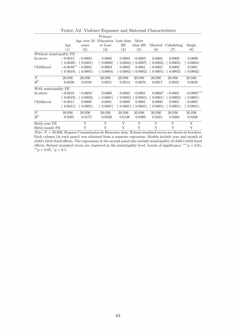
Table A2. Violence Exposure and Maternal Characteristics

AgeAge over 33

years

PrimaryEducation

or LessLess than

HSMore

than HS Married Cohabiting Single(1) (2) (3) (4) (5) (6) (7) (8)

Without municipality FEIn-utero −0.0012 −0.0002 0.0004 0.0002 −0.0003 0.0002 0.0000 0.0000

( 0.0020) ( 0.0001) ( 0.0008) ( 0.0002) ( 0.0007) ( 0.0002) ( 0.0005) ( 0.0004)Childhood −0.0040∗∗ −0.0002 −0.0003 0.0003 0.0001 −0.0002 0.0002 0.0001

( 0.0018) ( 0.0001) ( 0.0004) ( 0.0002) ( 0.0002) ( 0.0001) ( 0.0002) ( 0.0002)

N 20,936 20,936 20,936 20,936 20,936 20,936 20,936 20,936R2 0.0326 0.0108 0.0051 0.0014 0.0076 0.0017 0.0021 0.0038

With municipality FEIn-utero −0.0018 −0.0004∗ 0.0000 0.0002 −0.0001 0.0002∗ −0.0001 −0.0003∗∗∗

( 0.0019) ( 0.0002) ( 0.0001) ( 0.0002) ( 0.0001) ( 0.0001) ( 0.0002) ( 0.0001)Childhood −0.0011 0.0000 0.0001 0.0000 0.0001 0.0000 0.0001 −0.0001

( 0.0011) ( 0.0001) ( 0.0001) ( 0.0001) ( 0.0001) ( 0.0001) ( 0.0001) ( 0.0001)

N 20,936 20,936 20,936 20,936 20,936 20,936 20,936 20,936R2 0.0391 0.0175 0.0520 0.0126 0.0380 0.0221 0.0260 0.0326

Birth year FE Y Y Y Y Y Y YBirth month FE Y Y Y Y Y Y Y

Note: N = 20,936. Hogares Comunitarios de Bienestar data. Robust standard errors are shown in brackets.Each column (in each panel) was obtained from a separate regression. Models include year and month ofchild’s birth fixed effects. The regressions in the second panel also include municipality of child’s birth fixedeffects. Robust standard errors are clustered at the municipality level. Levels of significance: ∗∗∗p < 0.01,∗∗p < 0.05, ∗p < 0.1.

62

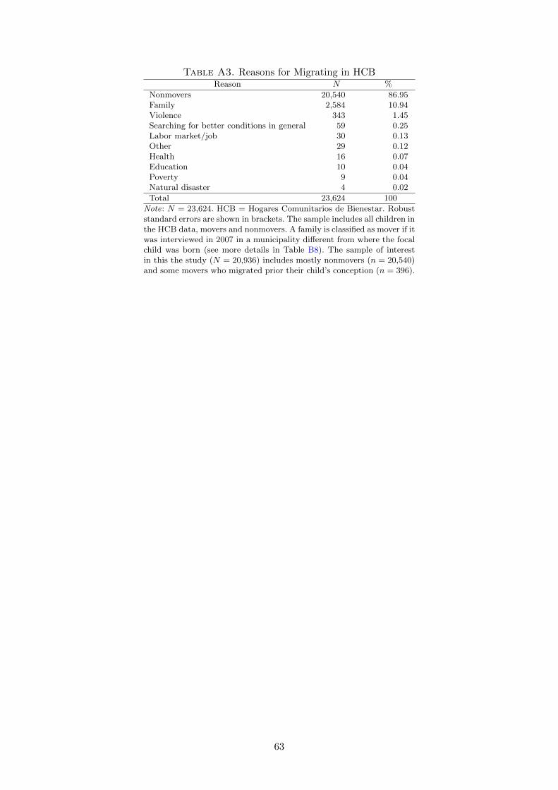
Table A3. Reasons for Migrating in HCBReason N %

Nonmovers 20,540 86.95Family 2,584 10.94Violence 343 1.45Searching for better conditions in general 59 0.25Labor market/job 30 0.13Other 29 0.12Health 16 0.07Education 10 0.04Poverty 9 0.04Natural disaster 4 0.02

Total 23,624 100

Note: N = 23,624. HCB = Hogares Comunitarios de Bienestar. Robuststandard errors are shown in brackets. The sample includes all children inthe HCB data, movers and nonmovers. A family is classified as mover if itwas interviewed in 2007 in a municipality different from where the focalchild was born (see more details in Table B8). The sample of interestin this the study (N = 20,936) includes mostly nonmovers (n = 20,540)and some movers who migrated prior their child’s conception (n = 396).

63

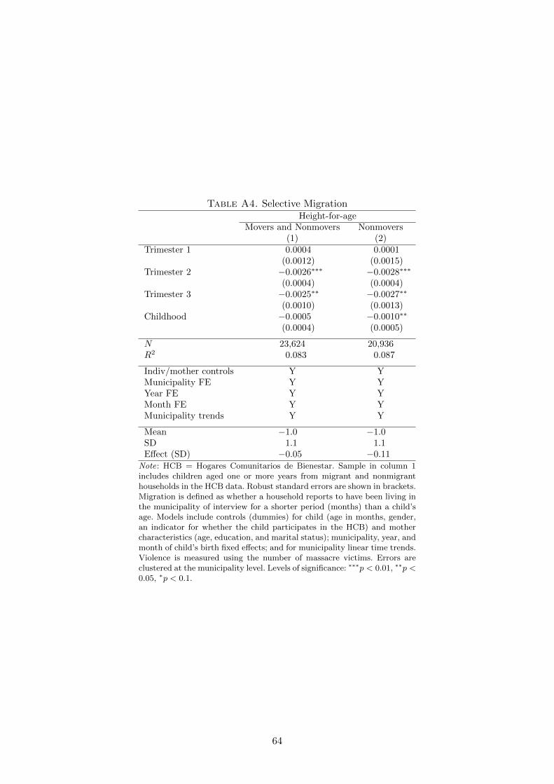
Table A4. Selective MigrationHeight-for-age

Movers and Nonmovers Nonmovers(1) (2)

Trimester 1 0.0004 0.0001(0.0012) (0.0015)

Trimester 2 −0.0026∗∗∗ −0.0028∗∗∗

(0.0004) (0.0004)Trimester 3 −0.0025∗∗ −0.0027∗∗

(0.0010) (0.0013)Childhood −0.0005 −0.0010∗∗

(0.0004) (0.0005)

N 23,624 20,936R2 0.083 0.087

Indiv/mother controls Y YMunicipality FE Y YYear FE Y YMonth FE Y YMunicipality trends Y Y

Mean −1.0 −1.0SD 1.1 1.1Effect (SD) −0.05 −0.11

Note: HCB = Hogares Comunitarios de Bienestar. Sample in column 1includes children aged one or more years from migrant and nonmigranthouseholds in the HCB data. Robust standard errors are shown in brackets.Migration is defined as whether a household reports to have been living inthe municipality of interview for a shorter period (months) than a child’sage. Models include controls (dummies) for child (age in months, gender,an indicator for whether the child participates in the HCB) and mothercharacteristics (age, education, and marital status); municipality, year, andmonth of child’s birth fixed effects; and for municipality linear time trends.Violence is measured using the number of massacre victims. Errors areclustered at the municipality level. Levels of significance: ∗∗∗p < 0.01, ∗∗p <0.05, ∗p < 0.1.

64

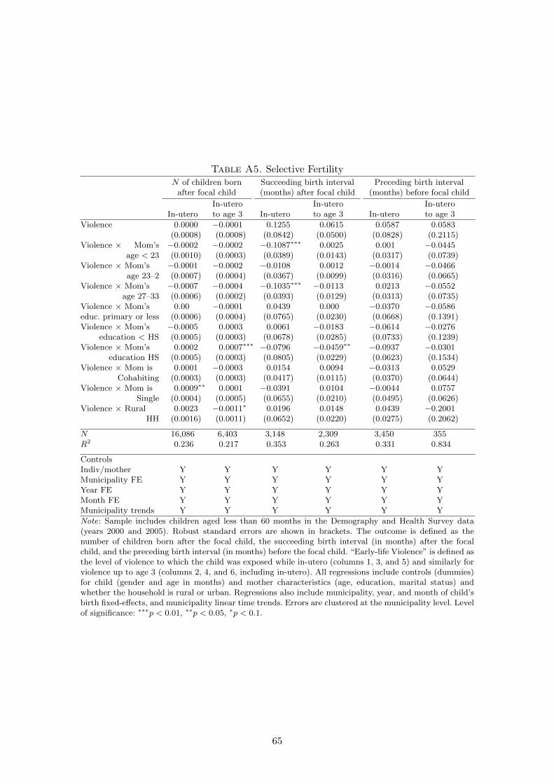
Table A5. Selective FertilityN of children born

after focal childSucceeding birth interval(months) after focal child

Preceding birth interval(months) before focal child

In-uteroIn-uteroto age 3 In-utero

In-uteroto age 3 In-utero

In-uteroto age 3

Violence 0.0000 −0.0001 0.1255 0.0615 0.0587 0.0583(0.0008) (0.0008) (0.0842) (0.0500) (0.0828) (0.2115)

Violence × Mom’s −0.0002 −0.0002 −0.1087∗∗∗ 0.0025 0.001 −0.0445age < 23 (0.0010) (0.0003) (0.0389) (0.0143) (0.0317) (0.0739)

Violence × Mom’s −0.0001 −0.0002 −0.0108 0.0012 −0.0014 −0.0466age 23–2 (0.0007) (0.0004) (0.0367) (0.0099) (0.0316) (0.0665)

Violence × Mom’s −0.0007 −0.0004 −0.1035∗∗∗ −0.0113 0.0213 −0.0552age 27–33 (0.0006) (0.0002) (0.0393) (0.0129) (0.0313) (0.0735)

Violence × Mom’s 0.00 −0.0001 0.0439 0.000 −0.0370 −0.0586educ. primary or less (0.0006) (0.0004) (0.0765) (0.0230) (0.0668) (0.1391)Violence × Mom’s −0.0005 0.0003 0.0061 −0.0183 −0.0614 −0.0276

education < HS (0.0005) (0.0003) (0.0678) (0.0285) (0.0733) (0.1239)Violence × Mom’s 0.0002 0.0007∗∗∗ −0.0796 −0.0459∗∗ −0.0937 −0.0301

education HS (0.0005) (0.0003) (0.0805) (0.0229) (0.0623) (0.1534)Violence × Mom is 0.0001 −0.0003 0.0154 0.0094 −0.0313 0.0529

Cohabiting (0.0003) (0.0003) (0.0417) (0.0115) (0.0370) (0.0644)Violence × Mom is 0.0009∗∗ 0.0001 −0.0391 0.0104 −0.0044 0.0757

Single (0.0004) (0.0005) (0.0655) (0.0210) (0.0495) (0.0626)Violence × Rural 0.0023 −0.0011∗ 0.0196 0.0148 0.0439 −0.2001

HH (0.0016) (0.0011) (0.0652) (0.0220) (0.0275) (0.2062)

N 16,086 6,403 3,148 2,309 3,450 355R2 0.236 0.217 0.353 0.263 0.331 0.834

ControlsIndiv/mother Y Y Y Y Y YMunicipality FE Y Y Y Y Y YYear FE Y Y Y Y Y YMonth FE Y Y Y Y Y YMunicipality trends Y Y Y Y Y Y

Note: Sample includes children aged less than 60 months in the Demography and Health Survey data(years 2000 and 2005). Robust standard errors are shown in brackets. The outcome is defined as thenumber of children born after the focal child, the succeeding birth interval (in months) after the focalchild, and the preceding birth interval (in months) before the focal child. “Early-life Violence” is defined asthe level of violence to which the child was exposed while in-utero (columns 1, 3, and 5) and similarly forviolence up to age 3 (columns 2, 4, and 6, including in-utero). All regressions include controls (dummies)for child (gender and age in months) and mother characteristics (age, education, marital status) andwhether the household is rural or urban. Regressions also include municipality, year, and month of child’sbirth fixed-effects, and municipality linear time trends. Errors are clustered at the municipality level. Levelof significance: ∗∗∗p < 0.01, ∗∗p < 0.05, ∗p < 0.1.

65

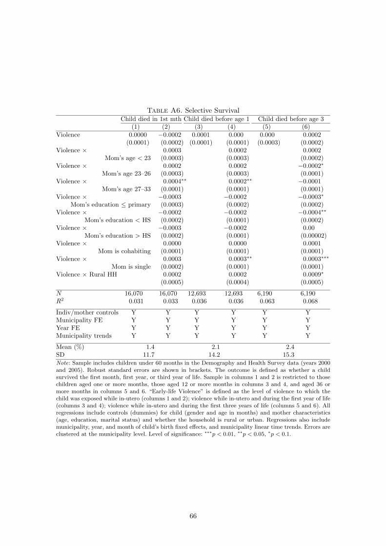
Table A6. Selective SurvivalChild died in 1st mth Child died before age 1 Child died before age 3

(1) (2) (3) (4) (5) (6)Violence 0.0000 −0.0002 0.0001 0.000 0.000 0.0002

(0.0001) (0.0002) (0.0001) (0.0001) (0.0003) (0.0002)Violence × 0.0003 0.0002 0.0002

Mom’s age < 23 (0.0003) (0.0003) (0.0002)Violence × 0.0002 0.0002 −0.0002∗

Mom’s age 23–26 (0.0003) (0.0003) (0.0001)Violence × 0.0004∗∗ 0.0002∗∗ −0.0001

Mom’s age 27–33 (0.0001) (0.0001) (0.0001)Violence × −0.0003 −0.0002 −0.0003∗

Mom’s education ≤ primary (0.0003) (0.0002) (0.0002)Violence × −0.0002 −0.0002 −0.0004∗∗

Mom’s education < HS (0.0002) (0.0001) (0.0002)Violence × −0.0003 −0.0002 0.00

Mom’s education > HS (0.0002) (0.0001) (0.00002)Violence × 0.0000 0.0000 0.0001

Mom is cohabiting (0.0001) (0.0001) (0.0001)Violence × 0.0003 0.0003∗∗ 0.0003∗∗∗

Mom is single (0.0002) (0.0001) (0.0001)Violence × Rural HH 0.0002 0.0002 0.0009∗

(0.0005) (0.0004) (0.0005)

N 16,070 16,070 12,693 12,693 6,190 6,190R2 0.031 0.033 0.036 0.036 0.063 0.068

Indiv/mother controls Y Y Y Y Y YMunicipality FE Y Y Y Y Y YYear FE Y Y Y Y Y YMunicipality trends Y Y Y Y Y Y

Mean (%) 1.4 2.1 2.4SD 11.7 14.2 15.3Note: Sample includes children under 60 months in the Demography and Health Survey data (years 2000and 2005). Robust standard errors are shown in brackets. The outcome is defined as whether a childsurvived the first month, first year, or third year of life. Sample in columns 1 and 2 is restricted to thosechildren aged one or more months, those aged 12 or more months in columns 3 and 4, and aged 36 ormore months in columns 5 and 6. “Early-life Violence” is defined as the level of violence to which thechild was exposed while in-utero (columns 1 and 2); violence while in-utero and during the first year of life(columns 3 and 4); violence while in-utero and during the first three years of life (columns 5 and 6). Allregressions include controls (dummies) for child (gender and age in months) and mother characteristics(age, education, marital status) and whether the household is rural or urban. Regressions also includemunicipality, year, and month of child’s birth fixed effects, and municipality linear time trends. Errors areclustered at the municipality level. Level of significance: ∗∗∗p < 0.01, ∗∗p < 0.05, ∗p < 0.1.

66

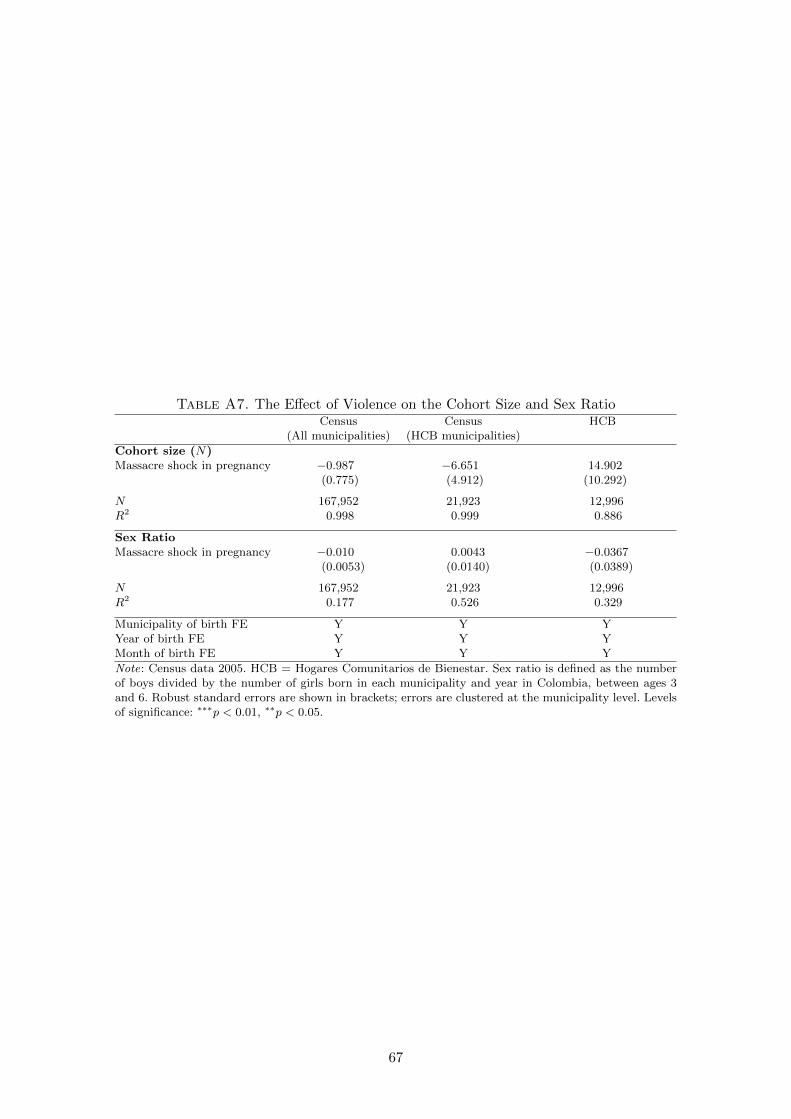
Table A7. The Effect of Violence on the Cohort Size and Sex RatioCensus Census HCB

(All municipalities) (HCB municipalities)

Cohort size (N)Massacre shock in pregnancy −0.987 −6.651 14.902

(0.775) (4.912) (10.292)

N 167,952 21,923 12,996R2 0.998 0.999 0.886

Sex RatioMassacre shock in pregnancy −0.010 0.0043 −0.0367

(0.0053) (0.0140) (0.0389)

N 167,952 21,923 12,996R2 0.177 0.526 0.329

Municipality of birth FE Y Y YYear of birth FE Y Y YMonth of birth FE Y Y Y

Note: Census data 2005. HCB = Hogares Comunitarios de Bienestar. Sex ratio is defined as the numberof boys divided by the number of girls born in each municipality and year in Colombia, between ages 3and 6. Robust standard errors are shown in brackets; errors are clustered at the municipality level. Levelsof significance: ∗∗∗p < 0.01, ∗∗p < 0.05.

67

B Additional Tables and Figures

As discussed in the data section, the sample of interest in this study comes from children of families who

have not migrated prior to the birth of the child. The reason for selecting the nonmovers and excluding

the mover sample is that the HCB does not provide information on the municipality of birth for children

of migrant families. Table B8 shows summary statistics for both children and mothers in the mover and

nonmover samples, which indicate that nonmover households tend to be a more advantaged group of

families than those who migrated at some point since child’s birth. Nonmigrant mothers are significantly

older and more educated than migrant mothers. They are also more likely to be married or to be single.

Children of nonmigrant families also report higher cognitive outcomes. These differences suggest that,

since the nonmover sample is a positively selected group in terms of mother and child characteristics, it

is likely that the estimates of violence on child outcomes for this group may result in a downward biased

coefficient of the true impact of violence.

68

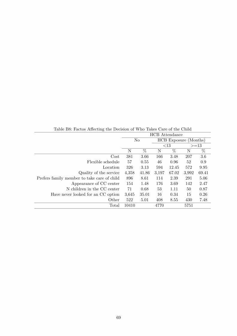
Table B8: Factos Affecting the Decision of Who Takes Care of the Child

HCB AttendanceNo HCB Exposure (Months)

<13 >=13N % N % N %

Cost 381 3.66 166 3.48 207 3.6Flexible schedule 57 0.55 46 0.96 52 0.9

Location 326 3.13 594 12.45 572 9.95Quality of the service 4,358 41.86 3,197 67.02 3,992 69.41

Prefers family member to take care of child 896 8.61 114 2.39 291 5.06Appearance of CC center 154 1.48 176 3.69 142 2.47

N children in the CC center 71 0.68 53 1.11 50 0.87Have never looked for an CC option 3,645 35.01 16 0.34 15 0.26

Other 522 5.01 408 8.55 430 7.48

Total 10410 4770 5751

69

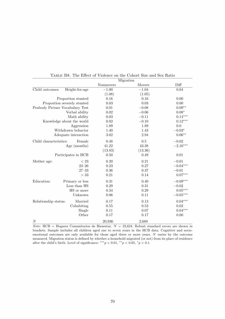
Table B8. The Effect of Violence on the Cohort Size and Sex RatioMigration

Nonmovers Movers DiffChild outcomes: Height-for-age −1.00 −1.04 0.04

(1.08) (1.05)Proportion stunted 0.16 0.16 0.00

Proportion severely stunted 0.03 0.03 0.00Peabody Picture Vocabulary Test 0.01 −0.08 0.09∗∗

Verbal ability 0.02 −0.06 0.08∗

Math ability 0.03 −0.11 0.14∗∗∗

Knowledge about the world 0.02 −0.10 0.12∗∗∗

Aggression 1.89 1.89 0.0Withdrawn behavior 1.40 1.43 −0.03∗

Adequate interaction 3.02 2.94 0.06∗∗

Child characteristics: Female 0.48 0.5 −0.02Age (months) 41.22 43.38 −2.16∗∗∗

(13.83) (13.36)Participates in HCB 0.50 0.49 0.01

Mother age: < 23 0.20 0.21 −0.0123–26 0.23 0.27 −0.04∗∗∗

27–33 0.36 0.37 −0.01> 33 0.21 0.14 0.07∗∗∗

Education: Primary or less 0.31 0.40 −0.09∗∗∗

Less than HS 0.29 0.31 −0.02HS or more 0.34 0.29 0.05∗∗∗

Unknown 0.06 0.11 −0.05∗∗∗

Relationship status: Married 0.17 0.13 0.04∗∗∗

Cohabiting 0.55 0.53 0.02Single 0.11 0.07 0.04∗∗∗

Other 0.17 0.17 0.00

N 20,936 2,688Note: HCB = Hogares Comunitarios de Bienestar. N = 23,624. Robust standard errors are shown inbrackets. Sample includes all children aged one to seven years in the HCB data. Cognitive and socio-emotional outcomes are only available for those aged three or more years. N varies by the outcomemeasured. Migration status is defined by whether a household migrated (or not) from its place of residenceafter the child’s birth. Level of significance: ∗∗∗p < 0.01, ∗∗p < 0.05, ∗p < 0.1.

70

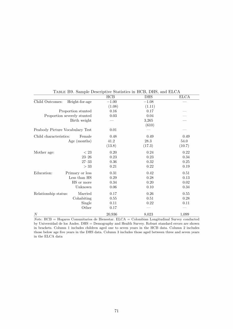
Table B9. Sample Descriptive Statistics in HCB, DHS, and ELCAHCB DHS ELCA

Child Outcomes: Height-for-age −1.00 −1.08 —(1.08) (1.11)

Proportion stunted 0.16 0.17 —Proportion severely stunted 0.03 0.04 —

Birth weight — 3,265 —(610)

Peabody Picture Vocabulary Test 0.01 — —

Child characteristics: Female 0.48 0.49 0.49Age (months) 41.2 28.3 54.0

(13.8) (17.3) (10.7)

Mother age: < 23 0.20 0.24 0.2223–26 0.23 0.23 0.3427–33 0.36 0.32 0.25> 33 0.21 0.22 0.19

Education: Primary or less 0.31 0.42 0.51Less than HS 0.29 0.28 0.13

HS or more 0.34 0.20 0.02Unknown 0.06 0.10 0.34

Relationship status: Married 0.17 0.26 0.55Cohabiting 0.55 0.51 0.28

Single 0.11 0.22 0.11Other 0.17 — —

N 20,936 8,023 1,099Note: HCB = Hogares Comunitarios de Bienestar. ELCA = Colombian Longitudinal Survey conductedby Universidad de los Andes. DHS = Demography and Health Survey. Robust standard errors are shownin brackets. Column 1 includes children aged one to seven years in the HCB data. Column 2 includesthose below age five years in the DHS data. Column 3 includes those aged between three and seven yearsin the ELCA data

71

C Other Microdata Sets

In addition to the HCB evaluation, this study uses other sources of microdata to provide additional

evidence of the pervasive effects of violence on child development. These other datasets constitute an

important contribution to this study for several reasons. First, because the HCB data was collected in

2007, year in which violence in Colombia had decreased substantially, I employ other sources of data that

allow me to measure child outcomes and potential mechanisms more closely to the period of more intense

violence and to the years in which my sample of children were born. Second, these datasets contain a much

larger sample of siblings compared to the HCB data. I am, therefore, able to calculate models that account

for mother time-invariant fixed effects, providing more compelling evidence of the impacts of violence on

human capital. Third, since these datasets have more national representation than the HCB data, they

also help me address the issue of external validity.

(1.) Demography and Health Survey (DHS): Standardized nationally representative (cross-sectional)

household surveys conducted in many developing countries. Interview women aged 15–49 years on

their health status, birth histories, fertility and use of family planning, and their demographic and

socioeconomic characteristics. The DHS also includes child anthropometric indicators (for those

below age of 5). I pool data from waves 1995, 2000, and 2005 to cover the most intense years of the

conflict.

(2.) Colombian Longitudinal Survey (ELCA by its Spanish acronym):36 First longitudinal survey in

Colombia with a sample of 4,000 rural and 6,000 urban households in different regions of the country.

The ELCA includes detailed modules on household characteristics such as health, education, labor-

market participation, wealth, and assets and provides information on child cognitive development.

I use the urban sample of the baseline wave (the only wave available), collected in 2010.

36Conducted by Universidad de los Andes in Bogota, Colombia.

72