energies

Article

Early Fault Detection of Wind Turbines Based onOperational Condition Clustering and OptimizedDeep Belief Network Modeling

Hong Wang * , Hongbin Wang, Guoqian Jiang , Jimeng Li and Yueling Wang

School of Electrical Engineering, Yanshan University, No. 438, Hebei Avenue, Qinhuangdao 066004, China;hb_wang@ysu.edu.cn (H.W.); jgqysu@gmail.com (G.J.); xjtuljm@163.com (J.L.); yuelingw@ysu.edu.cn (Y.W.)* Correspondence: hongw329@163.com

Received: 8 January 2019; Accepted: 7 March 2019; Published: 13 March 2019�����������������

Abstract: Health monitoring and early fault detection of wind turbines have attracted considerableattention due to the benefits of improving reliability and reducing the operation and maintenancecosts of the turbine. However, dynamic and constantly changing operating conditions of windturbines still pose great challenges to effective and reliable fault detection. Most existing healthmonitoring approaches mainly focus on one single operating condition, so these methods cannotassess the health status of turbines accurately, leading to unsatisfactory detection performance.To this end, this paper proposes a novel general health monitoring framework for wind turbinesbased on supervisory control and data acquisition (SCADA) data. A key feature of the proposedframework is that it first partitions the turbine operation into multiple sub-operation conditions bythe clustering approach and then builds a normal turbine behavior model for each sub-operationcondition. For normal behavior modeling, an optimized deep belief network is proposed. Thisoptimized modeling method can capture the sophisticated nonlinear correlations among differentmonitoring variables, which is helpful to enhance the prediction performance. A case study of mainbearing fault detection using real SCADA data is used to validate the proposed approach, whichdemonstrates its effectiveness and advantages.

Keywords: wind turbines; health monitoring; fault detection; optimized deep belief networks;supervisory control and data acquisition system; multioperation condition

1. Introduction

With increasing global energy demand, wind energy as a promising clean source of renewableenergy has become an indispensable force in solving world energy problems. The latest annualreport released by the Global Wind Energy Council (GWEC) [1] shows that the cumulative and newinstalled capacity in the world had reached 539,123 MW and 52,492 MW, respectively, by the end of2017. However, wind turbines are generally situated in remote locations and have harsh operatingenvironments, resulting in frequent failures and undesired shutdowns. High maintenance costs anddowntime losses seriously affect the economic benefits of wind farms and also have a powerful impacton the healthy development of the wind power industry [2]. There is an urgent need for effectiveprognostics and health management (PHM) technologies to address these problems. In particular,fault detection is a premise for PHM. Therefore, it is crucial and valuable to develop advanced healthmonitoring and fault detection methods to detect impending wind turbine faults as early as possiblein order to avoid secondary damage and even catastrophic accidents.

Vibration analysis and oil monitoring have become two commonly used techniques for windturbine condition monitoring [3–6]. However, both techniques are sophisticated and expensive in

Energies 2019, 12, 984; doi:10.3390/en12060984 www.mdpi.com/journal/energies

Energies 2019, 12, 984 2 of 22

their practical application, since additional investments, including installing extra sensors and dataacquisition devices, are required. Alternatively, supervisory control and data acquisition (SCADA)systems, which have been widely installed in large-scale wind turbines, can collect and record theoperational state information from wind turbines and their critical components on a regular basis [7].Compared with the vibration and oil monitoring methods, SCADA-based monitoring has beenconsidered to be cost-effective due to the availability of a large amount of monitoring data andno additional cost. As a result, SCADA-based wind turbine health monitoring has attracted wideattention in recent years [8], and different SCADA data analysis methods have been proposed.

Zaher et al. [9] developed normal behavior models for gearboxes and generators based on artificialneural networks by analyzing SCADA data. The case study results demonstrated that it was possible todetect faults as early as 6 months and 16 months before final replacement of the gearbox and generator,respectively. Guo et al. [10] employed a nonlinear state estimation method to construct a normalbehavior model of generator temperature using 2 min and 10 min averaged SCADA data. A real casestudy showed that the method was able to predict generator faults about 8.5 h before the actual failure.Kusiak et al. [11] introduced a neural network to model the normal behavior of generator bearingsby using 10 s SCADA data. The research showed that the method could identify anomalies about1.5 h ahead of the eventual failure. Schlechtingen et al. [12,13] proposed an adaptive neuro-fuzzyinference system combining artificial neural network and fuzzy logic analysis and constructed 45normal behavior models using 10 min averaged SCADA data. Case studies illustrated that thesystem could detect the potential failures of wind turbines months in advance and provide the rootcauses of these failures based on simple if–then rules. Bangalore et al. [14,15] applied artificial neuralnetworks to establish normal behavior models of gearboxes. Case studies with 10 min averagedSCADA data showed that the proposed methods were able to detect gearbox anomalies ahead ofthe condition monitoring system. Bi et al. [16] presented a pitch fault detection procedure using anormal behavior model based on the performance curve and carried out six case studies. The resultsillustrated that the proposed method could detect pitch faults earlier than the artificial intelligenceapproaches investigated. Different methods have been used to model the normal behavior of windturbines. Further, residuals between the predicted values of the models and actual measured valuesof the expected output variable were used to identify the anomalies of wind turbines. Practically,wind turbine operating conditions are complicated and changeable and present multiple operationregions due to varying external wind speed and a complex internal control scheme, which poses greatchallenges for effective and reliable fault detection. However, most existing monitoring approachesonly focus on a single whole operating condition, so they cannot fully consider the dynamic operatingcharacteristics of wind turbines, leading to unsatisfactory detection performance, such as high rates offalse alarms or missed detections. On the other hand, conventional health monitoring methods, suchas neural networks, naturally have classical shallow structures, which poses a difficulty in effectivelycapturing sophisticated nonlinear relationships among monitoring variables.

To address the above issues, a novel general health monitoring approach for wind turbines undervarying operating conditions is proposed in this paper. This approach is data-driven and based onmonitoring data collected from wind turbine SCADA systems. First, to consider the dynamic behaviorand multiple operating characteristics of wind turbines, an operation condition partition schemeusing a clustering algorithm is proposed to partition the whole operation into multiple sub-operationconditions. This is a divide-and-conquer strategy and can enable the building of local monitoringmodels in different sub-operation conditions, which can improve the reliability and accuracy of faultdetection compared to a global monitoring model. Second, to overcome the shortcoming of traditionalshallow structure–based methods, a deep learning–based modeling approach is proposed to deal withrelevant SCADA data to capture the sophisticated nonlinear correlations among monitoring variables.In recent years, motivated by the powerful ability of feature learning and nonlinear modeling of deeplearning methods, convolutional neural network [17], autoencoder [18], denoising autoencoder [19],and multilayered extreme learning machines [20] have been used in many classification and regression

Energies 2019, 12, 984 3 of 22

tasks. Specifically, deep belief networks (DBNs) [21], a typical class of deep learning methods, areused in this study, which are naturally probabilistic generative models with multilayered architecture.Compared with shallow neural network methods, DBNs can capture complex nonlinear features,have a powerful modeling capacity and are quite suitable for modeling complex SCADA data [22].DBNs have received attention in the fields of wind speed prediction [23], mechanical engineeringfault diagnosis [24] and complex system fault detection [25]. The performance of DBNs is largelydependent on their structural parameters. However, there is no uniform rule for parameter selection.Various optimization algorithms have shown the ability to deal with complex problems, such asparticle swarm [26] and genetic algorithm [27]. In particular, chicken swarm optimization (CSO), anovel bionic heuristic optimization algorithm, is introduced for optimizing model parameters of DBNs.In summary, the main contributions of this paper are as follows:

(1) A general multioperation condition partition scheme is proposed to partition normal state datainto several different clusters. Then, normal behaviors are built under different condition clusters.This divide-and-conquer strategy can help reduce false alarms caused by methods that onlyconsider a single operating condition.

(2) An optimized DBN (ODBN) model with CSO is designed to capture the normal behavior ineach cluster, which reduces the complexity of parameter selection of DBNs. To the best of ourknowledge, it is the first time DBN is applied to deal with complex SCADA data from windturbines for the purpose of fault detection.

(3) A real case from wind turbine main bearing fault was used to evaluate the performance of theproposed health monitoring approach using the SCADA data of multiple wind turbines from areal wind farm, and comparative studies were conducted.

The remainder of this paper is organized as follows. Section 2 describes the multioperationcondition problem and the operation parameters studied in this paper. In Section 3, the proposedhealth monitoring framework is presented, the steps are explained, and the presented methodologiesare described in detail. Section 4 presents the case study and discussion, and results are compared andanalyzed. Conclusions are summarized in Section 5.

2. Problem Description

As critical equipment for wind power generation, a wind turbine is typically a complexelectromechanical system composed of a variety of components and subsystems, including gearbox,generator, shaft, bearing, and power electronics, among many others [28]. In practical applications,wind turbines are generally located in remote areas and perennially operate under adverse weatherconditions, such as storms, dust, and extreme temperature differentials. In addition, they are alsoaffected by mechanical, electrical, and control strategies. These kinds of situations lead to operatingconditions characterized by complexity and variability. As discussed in the first section, one of theprimary disadvantages of existing data-driven condition monitoring approaches for wind turbines isthat they only take into account a single operating condition, ignoring the characteristics that exist inthe process of operating wind turbines. Due to their highly dynamic operating conditions, variationsin the abnormal states of turbines are always easily masked by the condition fluctuations, making itdifficult to accurately assess the health status and thereby causing frequent false alarms. In this case, itis highly desirable to develop reliable health monitoring approaches to deal with the dynamic andvarying operating conditions of wind turbines.

Wind turbine SCADA data contain hundreds of monitoring parameters related to the health ofthe wind turbine and its critical components. Typically, these parameters include wind conditions(e.g., wind speed, wind direction), power output, blade pitch angle, generator torque and speed,temperatures (e.g., main bearing temperature, gearbox oil temperature, nacelle temperature, andambient temperature) among others [29]. Several parameters are closely related to the wind turbineoperating conditions, which can be referred to as operation parameters, describing the external

Energies 2019, 12, 984 4 of 22

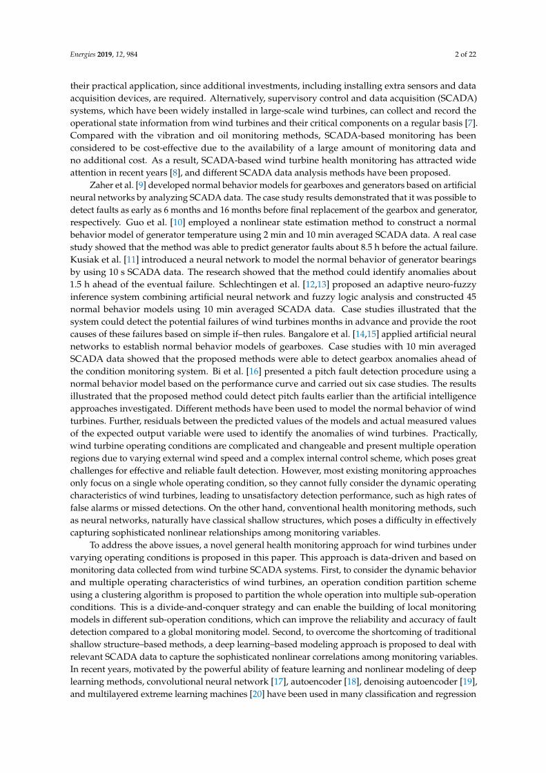
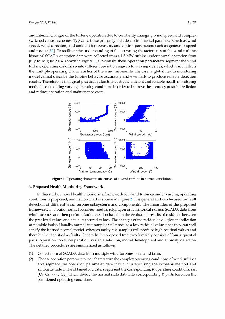
and internal changes of the turbine operation due to constantly changing wind speed and complexswitched control schemes. Typically, these primarily include environmental parameters such as windspeed, wind direction, and ambient temperature, and control parameters such as generator speedand torque [30]. To facilitate the understanding of the operating characteristics of the wind turbine,historical SCADA operation data were collected from a 1.5 MW turbine under normal operation fromJuly to August 2014, shown in Figure 1. Obviously, these operation parameters segment the windturbine operating conditions into different operation regions to varying degrees, which truly reflectsthe multiple operating characteristics of the wind turbine. In this case, a global health monitoringmodel cannot describe the turbine behavior accurately and even fails to produce reliable detectionresults. Therefore, it is of great practical value to investigate efficient and reliable health monitoringmethods, considering varying operating conditions in order to improve the accuracy of fault predictionand reduce operation and maintenance costs.

Energies 2019, 12, 984 4 of 22

speed and torque [30]. To facilitate the understanding of the operating characteristics of the wind turbine, historical SCADA operation data were collected from a 1.5 MW turbine under normal operation from July to August 2014, shown in Figure 1. Obviously, these operation parameters segment the wind turbine operating conditions into different operation regions to varying degrees, which truly reflects the multiple operating characteristics of the wind turbine. In this case, a global health monitoring model cannot describe the turbine behavior accurately and even fails to produce reliable detection results. Therefore, it is of great practical value to investigate efficient and reliable health monitoring methods, considering varying operating conditions in order to improve the accuracy of fault prediction and reduce operation and maintenance costs.

Figure 1. Operating characteristic curves of a wind turbine in normal conditions.

3. Proposed Health Monitoring Framework

In this study, a novel health monitoring framework for wind turbines under varying operating conditions is proposed, and its flowchart is shown in Figure 2. It is general and can be used for fault detection of different wind turbine subsystems and components. The main idea of the proposed framework is to build normal behavior models relying on only historical normal SCADA data from wind turbines and then perform fault detection based on the evaluation results of residuals between the predicted values and actual measured values. The changes of the residuals will give an indication of possible faults. Usually, normal test samples will produce a low residual value since they can well satisfy the learned normal model, whereas faulty test samples will produce high residual values and therefore be identified as faults. Generally, the proposed framework mainly consists of four sequential parts: operation condition partition, variable selection, model development and anomaly detection. The detailed procedures are summarized as follows:

(1) Collect normal SCADA data from multiple wind turbines on a wind farm. (2) Choose operation parameters that characterize the complex operating conditions of wind

turbines and segment the operation parameter data into K clusters using the k-means method and silhouette index. The obtained K clusters represent the corresponding K operating conditions, i.e., 1 2[ , , , ]KC C C . Then, divide the normal state data into corresponding K parts based on the partitioned operating conditions.

(3) Select appropriate modeling variables for each operating condition by combining three variable selection techniques, and the final selected variables for different operating clusters can be represented as 1 2[ , , , ]KV V V .

(4) Build a normal behavior model under each operating condition using ODBNs to explore the sophisticated nonlinear characteristics among modeling variables, resulting in multiple DBN models, denoted as 1 2[DBN , DBN , , DBN ]K for K operating clusters.

0 1000 2000-5000

0

5000

10,000

Generator speed (rpm)

Gen

era

tor

torq

ue

(N·m

)

0 10 20-5000

0

5000

10,000

Wind speed (m/s)

Gen

era

tor

torq

ue

(N·m

)

0 10 20 30-5000

0

5000

10,000

Ambient temperature (°C)

Ge

nera

tor

torq

ue

(N

·m)

0 200 400-5000

0

5000

10,000

Wind direction (°)

Ge

nera

tor

torq

ue

(N

·m)

Figure 1. Operating characteristic curves of a wind turbine in normal conditions.

3. Proposed Health Monitoring Framework

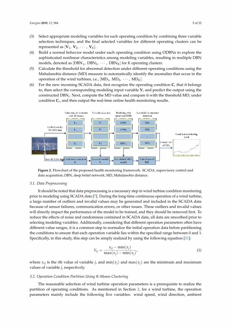
In this study, a novel health monitoring framework for wind turbines under varying operatingconditions is proposed, and its flowchart is shown in Figure 2. It is general and can be used for faultdetection of different wind turbine subsystems and components. The main idea of the proposedframework is to build normal behavior models relying on only historical normal SCADA data fromwind turbines and then perform fault detection based on the evaluation results of residuals betweenthe predicted values and actual measured values. The changes of the residuals will give an indicationof possible faults. Usually, normal test samples will produce a low residual value since they can wellsatisfy the learned normal model, whereas faulty test samples will produce high residual values andtherefore be identified as faults. Generally, the proposed framework mainly consists of four sequentialparts: operation condition partition, variable selection, model development and anomaly detection.The detailed procedures are summarized as follows:

(1) Collect normal SCADA data from multiple wind turbines on a wind farm.(2) Choose operation parameters that characterize the complex operating conditions of wind turbines

and segment the operation parameter data into K clusters using the k-means method andsilhouette index. The obtained K clusters represent the corresponding K operating conditions, i.e.,[C1, C2, · · · , CK]. Then, divide the normal state data into corresponding K parts based on thepartitioned operating conditions.

Energies 2019, 12, 984 5 of 22

(3) Select appropriate modeling variables for each operating condition by combining three variableselection techniques, and the final selected variables for different operating clusters can berepresented as [V1, V2, · · · , VK].

(4) Build a normal behavior model under each operating condition using ODBNs to explore thesophisticated nonlinear characteristics among modeling variables, resulting in multiple DBNmodels, denoted as [DBN 1, DBN2, · · · , DBNK] for K operating clusters.

(5) Calculate the threshold for abnormal detection under different operating conditions using theMahalanobis distance (MD) measure to automatically identify the anomalies that occur in theoperation of the wind turbines, i.e., [MD1, MD2, · · · , MDK].

(6) For the new incoming SCADA data, first recognize the operating condition Ci that it belongsto, then select the corresponding modeling input variable Vi and predict the output using theconstructed DBNi. Next, compute the MD value and compare it with the threshold MDi undercondition Ci, and then output the real-time online health monitoring results.

Figure 2. Flowchart of the proposed health monitoring framework. SCADA, supervisory control anddata acquisition; DBN, deep belief network; MD, Mahalanobis distance.

3.1. Data Preprocessing

It should be noted that data preprocessing is a necessary step in wind turbine condition monitoringprior to modeling using SCADA data [7]. During the long-time continuous operation of a wind turbine,a large number of outliers and invalid values may be generated and included in the SCADA databecause of sensor failures, communication errors, or other issues. These outliers and invalid valueswill directly impact the performance of the model to be trained, and they should be removed first. Toreduce the effects of noise and randomness contained in SCADA data, all data are smoothed prior toselecting modeling variables. Additionally, considering that different operation parameters often havedifferent value ranges, it is a common step to normalize the initial operation data before partitioningthe conditions to ensure that each operation variable lies within the specified range between 0 and 1.Specifically, in this study, this step can be simply realized by using the following equation [31]:

Yij =xij −min(xj)

max(xj)−min(xj), (1)

where xij is the ith value of variable j, and min(xj) and max(xj) are the minimum and maximumvalues of variable j, respectively.

3.2. Operation Condition Partition Using K-Means Clustering

The reasonable selection of wind turbine operation parameters is a prerequisite to realize thepartition of operating conditions. As mentioned in Section 2, for a wind turbine, the operationparameters mainly include the following five variables: wind speed, wind direction, ambient

Energies 2019, 12, 984 6 of 22

temperature, generator speed, and generator torque, which are closely related to the operatingconditions. Generally, the operating conditions can be partitioned into several typical operationregions depending on the above operation parameters. As an unsupervised learning method, k-meansclustering [32] has become one of the most prevalent and widely used partitioning clustering algorithmsdue to its advantages of usability, efficiency, simplicity and successful experience [33]. Hence, in thisstudy, this method is adopted for the condition partition. Certainly, other clustering methods can alsobe considered. The aim of k-means is to allocate all data samples into K clusters by minimizing thesum of the squared error over all K clusters, denoted as follows [33]:

J = arg minO

K

∑i=1

∑xj∈Oi

∥∥xj − µi∥∥2, (2)

where O = {O1, O2, . . . , OK} is the set of K clusters, µi is the cluster centroid of the ith cluster,{x1, x2, . . . , xN} is the cluster samples, and N is the number of samples.

In the k-means algorithm, the number of clusters K is a key parameter. Silhouette [34] is oneof the indices for evaluating the clustering number by combining the two factors of cohesion andresolution, which is employed to determine K in this paper. The silhouette value for the ith point, S(i),is expressed as

S(i) =b(i)−a(i)

max{a(i), b(i)} , i = 1, 2, . . . , N, (3)

where a(i) represents the average distance from the ith point to the other points in the same clusterand b(i) denotes the minimum average distance from the point to points in a different cluster. Therange of S(i) is [–1, 1]. A higher value of S(i) indicates that the ith point is clustered more properly.The average of all S(i) is then the final silhouette value for a given cluster number.

3.3. Variable Selection

To construct the normal behavior model, it is necessary to first determine the modeling variablesin each operating condition. Usually, there are multiple types of relationship among the variablesand various techniques can be applied to assess each type of relationship [35]. Three typicalvariable selection techniques are proposed in [36–38], the Pearson, Spearman, and Kendall correlationcoefficients, which are statistics for measuring the linearity, monotonicity, and dependence amongvariables, respectively. This paper combines the three technologies to select the input variables mostrelevant to the output variables. It is worth noting that the computation results of these three methodsare all in the range of –1 to 1, and a higher absolute value indicates a stronger correlation between theinput and output.

3.4. Proposed ODBN Method

The use of wind turbine SCADA systems becomes the primary option for most wind farms,and as a result, large amounts of monitoring data can be acquired and archived regularly. Themeasured SCADA data have notable features of complex nonlinearity and strong coupling due tothe interdependence and interaction between the different subsystems of the wind turbines duringoperation. Consequently, in this section, ODBNs are proposed to capture the latent nonlinearcorrelations in the SCADA monitoring data, and the details are described as follows.

3.4.1. DBN Architecture

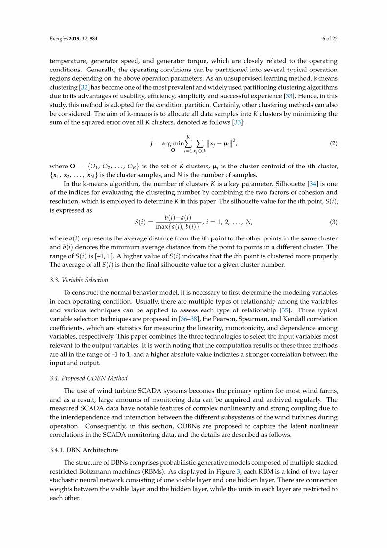
The structure of DBNs comprises probabilistic generative models composed of multiple stackedrestricted Boltzmann machines (RBMs). As displayed in Figure 3, each RBM is a kind of two-layerstochastic neural network consisting of one visible layer and one hidden layer. There are connectionweights between the visible layer and the hidden layer, while the units in each layer are restricted toeach other.

Energies 2019, 12, 984 7 of 22

Figure 3. Topological structure of a restricted Boltzmann machine (RBM).

Assuming that the RBM is a Bernoulli–Bernoulli model (BB-RBM), for a given set of states (v, h),the energy function is defined as

E(v, h; θ) = −V

∑i=1

H

∑j=1

ωijvihj −V

∑i=1

bivi −H

∑j=1

ajhj, (4)

where θ = {w, a, b} denotes the model parameters; vi and hj are the visible unit i and the hidden unitj, respectively; ωij is the connection weight between i and j; bi and aj are the biases of vi and hj; and Vand H are the number of visible and hidden units, respectively. Given the energy function, the jointprobability over the visible and hidden units can be described as follows:

p(v, h; θ) =1Z

exp(−E(v, h; θ)), (5)

where Z = ∑v

∑h

exp(−E(v, h; θ)) is the partition function.

Since the visible–visible and hidden–hidden units are not connected, the probabilities of thevisible unit vi and the hidden unit hj are independent. Therefore, the conditional distributions can beexpressed as

p(hj = 1|v; θ ) = δ(V

∑i=1

ωijvi + aj), (6)

p(vi = 1|h; θ ) = δ(H

∑j=1

ωijhj + bi), (7)

where δ(x) = 1/(1 + exp(x)) represents the logistic sigmoid function. The model parameters θ of theRBM can be obtained by a contrastive divergence method [39]. The update rule for the weight w iswritten as follows:

∆ωij = ε(⟨

vihj⟩

data −⟨vihj

⟩k), (8)

where ε refers to the learning rate, 〈·〉data denotes the expectation of the training data, and 〈·〉k representsthe expectation of the sample distribution after k-step Gibbs sampling. A more detailed description ofthe training process of the RBM can be seen in [40].

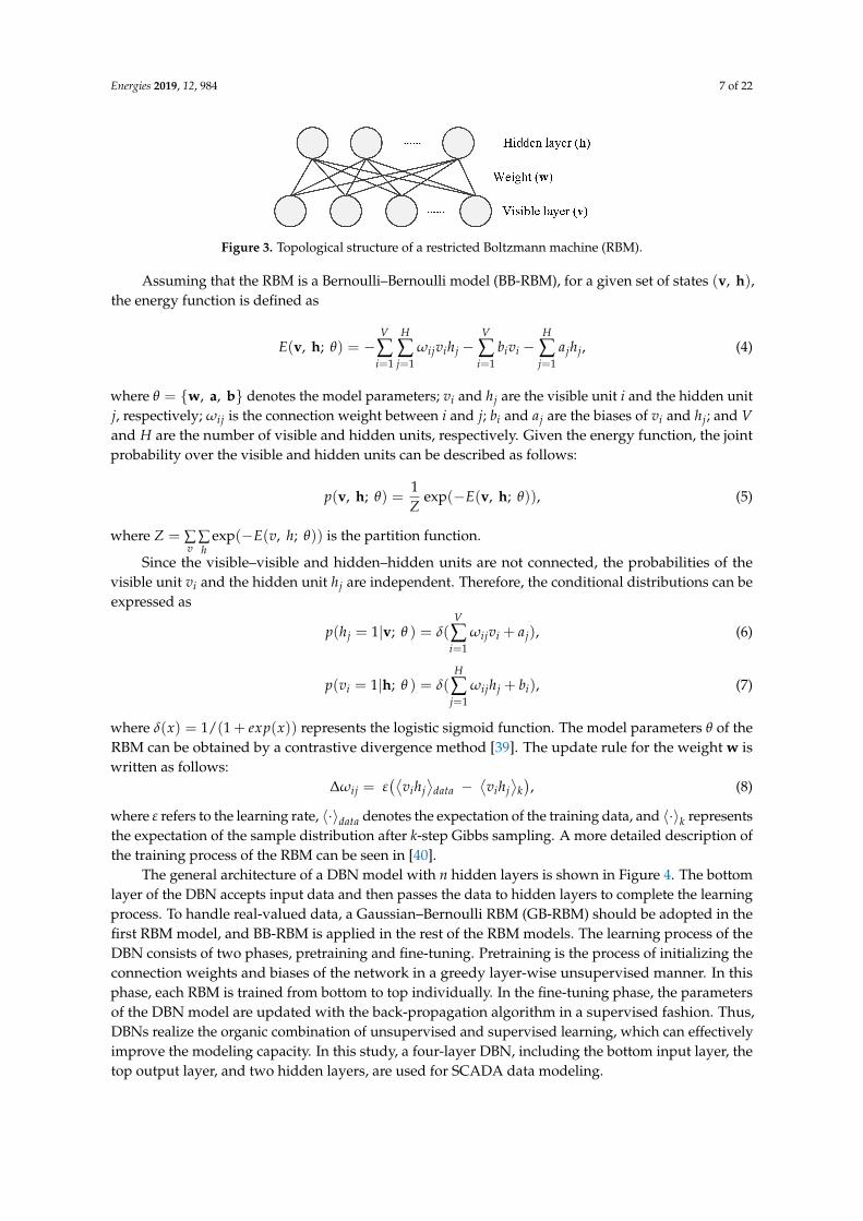
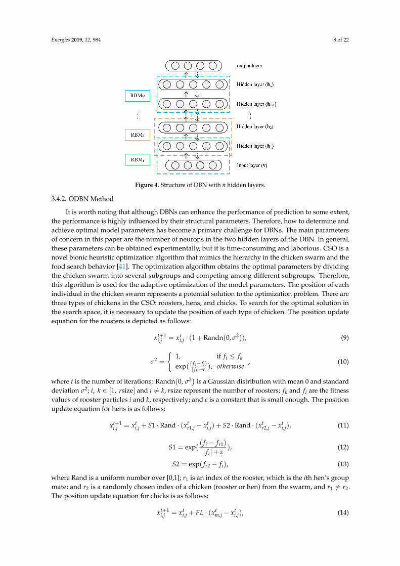
The general architecture of a DBN model with n hidden layers is shown in Figure 4. The bottomlayer of the DBN accepts input data and then passes the data to hidden layers to complete the learningprocess. To handle real-valued data, a Gaussian–Bernoulli RBM (GB-RBM) should be adopted in thefirst RBM model, and BB-RBM is applied in the rest of the RBM models. The learning process of theDBN consists of two phases, pretraining and fine-tuning. Pretraining is the process of initializing theconnection weights and biases of the network in a greedy layer-wise unsupervised manner. In thisphase, each RBM is trained from bottom to top individually. In the fine-tuning phase, the parametersof the DBN model are updated with the back-propagation algorithm in a supervised fashion. Thus,DBNs realize the organic combination of unsupervised and supervised learning, which can effectivelyimprove the modeling capacity. In this study, a four-layer DBN, including the bottom input layer, thetop output layer, and two hidden layers, are used for SCADA data modeling.

Energies 2019, 12, 984 8 of 22

Figure 4. Structure of DBN with n hidden layers.

3.4.2. ODBN Method

It is worth noting that although DBNs can enhance the performance of prediction to some extent,the performance is highly influenced by their structural parameters. Therefore, how to determine andachieve optimal model parameters has become a primary challenge for DBNs. The main parametersof concern in this paper are the number of neurons in the two hidden layers of the DBN. In general,these parameters can be obtained experimentally, but it is time-consuming and laborious. CSO is anovel bionic heuristic optimization algorithm that mimics the hierarchy in the chicken swarm and thefood search behavior [41]. The optimization algorithm obtains the optimal parameters by dividingthe chicken swarm into several subgroups and competing among different subgroups. Therefore,this algorithm is used for the adaptive optimization of the model parameters. The position of eachindividual in the chicken swarm represents a potential solution to the optimization problem. There arethree types of chickens in the CSO: roosters, hens, and chicks. To search for the optimal solution inthe search space, it is necessary to update the position of each type of chicken. The position updateequation for the roosters is depicted as follows:

xt+1i,j = xt

i,j · (1 + Randn(0, σ2)), (9)

σ2 =

{1, if fi ≤ fk

exp( ( fk− fi)| fi |+ε

), otherwise, (10)

where t is the number of iterations; Randn(0, σ2) is a Gaussian distribution with mean 0 and standarddeviation σ2; i, k ∈ [1, rsize] and i 6= k, rsize represent the number of roosters; fk and fi are the fitnessvalues of rooster particles i and k, respectively; and ε is a constant that is small enough. The positionupdate equation for hens is as follows:

xt+1i,j = xt

i,j + S1 · Rand · (xtr1,j − xt

i,j) + S2 · Rand · (xtr2,j − xt

i,j), (11)

S1 = exp(( fi − fr1)

| fi|+ ε), (12)

S2 = exp( fr2 − fi), (13)

where Rand is a uniform number over [0,1]; r1 is an index of the rooster, which is the ith hen’s groupmate; and r2 is a randomly chosen index of a chicken (rooster or hen) from the swarm, and r1 6= r2.The position update equation for chicks is as follows:

xt+1i,j = xt

i,j + FL · (xtm,j − xt

i,j), (14)

Energies 2019, 12, 984 9 of 22

where FL refers to a parameter that means the chick would follow its mother to forage for food, andthe range is [0, 2]; and xt

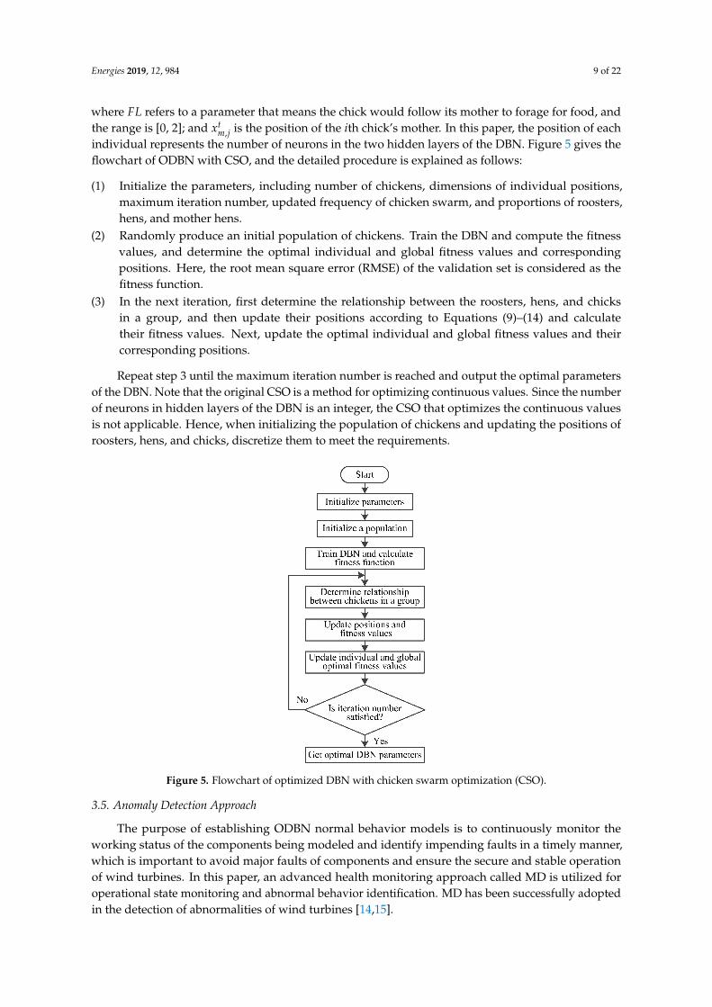
m,j is the position of the ith chick’s mother. In this paper, the position of eachindividual represents the number of neurons in the two hidden layers of the DBN. Figure 5 gives theflowchart of ODBN with CSO, and the detailed procedure is explained as follows:

(1) Initialize the parameters, including number of chickens, dimensions of individual positions,maximum iteration number, updated frequency of chicken swarm, and proportions of roosters,hens, and mother hens.

(2) Randomly produce an initial population of chickens. Train the DBN and compute the fitnessvalues, and determine the optimal individual and global fitness values and correspondingpositions. Here, the root mean square error (RMSE) of the validation set is considered as thefitness function.

(3) In the next iteration, first determine the relationship between the roosters, hens, and chicksin a group, and then update their positions according to Equations (9)–(14) and calculatetheir fitness values. Next, update the optimal individual and global fitness values and theircorresponding positions.

Repeat step 3 until the maximum iteration number is reached and output the optimal parametersof the DBN. Note that the original CSO is a method for optimizing continuous values. Since the numberof neurons in hidden layers of the DBN is an integer, the CSO that optimizes the continuous valuesis not applicable. Hence, when initializing the population of chickens and updating the positions ofroosters, hens, and chicks, discretize them to meet the requirements.

Figure 5. Flowchart of optimized DBN with chicken swarm optimization (CSO).

3.5. Anomaly Detection Approach

The purpose of establishing ODBN normal behavior models is to continuously monitor theworking status of the components being modeled and identify impending faults in a timely manner,which is important to avoid major faults of components and ensure the secure and stable operationof wind turbines. In this paper, an advanced health monitoring approach called MD is utilized foroperational state monitoring and abnormal behavior identification. MD has been successfully adoptedin the detection of abnormalities of wind turbines [14,15].

Energies 2019, 12, 984 10 of 22

MD is a unitless distance measurement that can capture the correlation of variables in a processor system and is defined as follows:

MDi =

√(Xi − µ)C−1(Xi − µ)T , i = 1, 2, . . . , n, (15)

where Xi = [Xi1, Xi2, . . . , Xim] is the ith observation vector, n is the number of observations, m is thetotal number of parameters, µ = [µ1, µ2, . . . , µm] is the vector of mean values, C is the covariancematrix, and MDi is the MD value for the ith vector Xi.

For health monitoring, the MD values for the validation set are used to calculate the thresholdfor anomaly detection. During the validation stage, wind turbines are in normal operation and noabnormal behavior occurs. The MD for the validation set can be expressed as follows:

MDre f i =√(Xre f i − µre f )C−1

re f (Xre f i − µre f )T, (16)

where Xre f i = [VEi, TVi] represents the ith vector; TVi denotes the ith target value during thevalidation stage and VEi is the corresponding validation error; µre f and Cre f are the mean value vectorand the covariance matrix of Xre f , respectively. MDre f i refers to the MD value for the ith vector Xre f i.

After obtaining the healthy MD values in the validation stage, the anomaly detection thresholdcan be determined by fitting a two-parameter Weibull probability distribution function on these MDvalues [42]. The two-parameter Weibull distribution is described as

f (t) = βη−β(t)β−1e−(tη )

β

, (17)

where β denotes the shape parameter and η stands for the scale parameter.The MD during the condition monitoring stage is depicted as follows:

MDnewi =√(Xnewi − µre f )C−1

re f (Xnewi − µre f )T, (18)

where Xnewi = [PEi, MVi], MVi is the ith actual measured value from the SCADA system during thecondition monitoring stage, and PEi is the model prediction error.

In this study, in order to reduce the false alarm rate, the MD value from the condition monitoringstage is identified as an anomaly if f (MDnewi) is less than 0.1%. At this point, an alarm signal istriggered to alert the operators about the operational states of the turbine so they can take appropriateaction to avoid major faults.

4. Case Study and Discussion

In this section, a real case for main bearings is investigated to demonstrate the feasibility ofthe proposed approach in practical applications of wind turbine health monitoring, and the resultsobtained in each part are presented in detail.

4.1. Data Description

The SCADA data used in this paper are from a wind farm located in Inner Mongolia, China. Allwind turbines in the wind farm are variable speed constant frequency with a rated power of 1.5 MW.The sampling interval of the SCADA data is 30 s. Each record includes a total of 25 discrete piecesof information, such as turbine state, time stamp, yaw state, etc. At the same time, 49 continuousparameters are also recorded, listed in Table 1. The SCADA data for the majority of the turbines wereavailable during the period from 1 July to 23 September 2014. In this paper, the SCADA data from 13available turbines during the period 1 July to 31 August 2014 are investigated. Detailed descriptions ofthe datasets are listed in Table 2.

Energies 2019, 12, 984 11 of 22

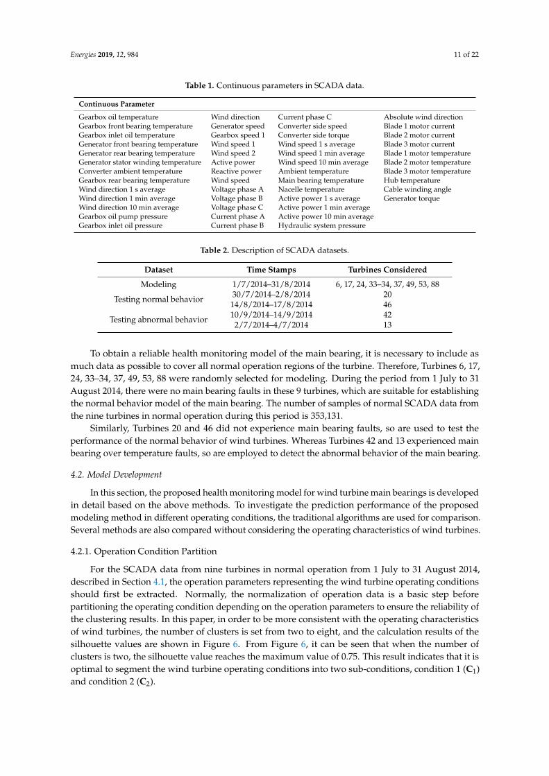
Table 1. Continuous parameters in SCADA data.

Continuous Parameter

Gearbox oil temperature Wind direction Current phase C Absolute wind directionGearbox front bearing temperature Generator speed Converter side speed Blade 1 motor currentGearbox inlet oil temperature Gearbox speed 1 Converter side torque Blade 2 motor currentGenerator front bearing temperature Wind speed 1 Wind speed 1 s average Blade 3 motor currentGenerator rear bearing temperature Wind speed 2 Wind speed 1 min average Blade 1 motor temperatureGenerator stator winding temperature Active power Wind speed 10 min average Blade 2 motor temperatureConverter ambient temperature Reactive power Ambient temperature Blade 3 motor temperatureGearbox rear bearing temperature Wind speed Main bearing temperature Hub temperatureWind direction 1 s average Voltage phase A Nacelle temperature Cable winding angleWind direction 1 min average Voltage phase B Active power 1 s average Generator torqueWind direction 10 min average Voltage phase C Active power 1 min averageGearbox oil pump pressure Current phase A Active power 10 min averageGearbox inlet oil pressure Current phase B Hydraulic system pressure

Table 2. Description of SCADA datasets.

Dataset Time Stamps Turbines Considered

Modeling 1/7/2014–31/8/2014 6, 17, 24, 33–34, 37, 49, 53, 88

Testing normal behavior 30/7/2014–2/8/2014 2014/8/2014–17/8/2014 46

Testing abnormal behavior 10/9/2014–14/9/2014 422/7/2014–4/7/2014 13

To obtain a reliable health monitoring model of the main bearing, it is necessary to include asmuch data as possible to cover all normal operation regions of the turbine. Therefore, Turbines 6, 17,24, 33–34, 37, 49, 53, 88 were randomly selected for modeling. During the period from 1 July to 31August 2014, there were no main bearing faults in these 9 turbines, which are suitable for establishingthe normal behavior model of the main bearing. The number of samples of normal SCADA data fromthe nine turbines in normal operation during this period is 353,131.

Similarly, Turbines 20 and 46 did not experience main bearing faults, so are used to test theperformance of the normal behavior of wind turbines. Whereas Turbines 42 and 13 experienced mainbearing over temperature faults, so are employed to detect the abnormal behavior of the main bearing.

4.2. Model Development

In this section, the proposed health monitoring model for wind turbine main bearings is developedin detail based on the above methods. To investigate the prediction performance of the proposedmodeling method in different operating conditions, the traditional algorithms are used for comparison.Several methods are also compared without considering the operating characteristics of wind turbines.

4.2.1. Operation Condition Partition

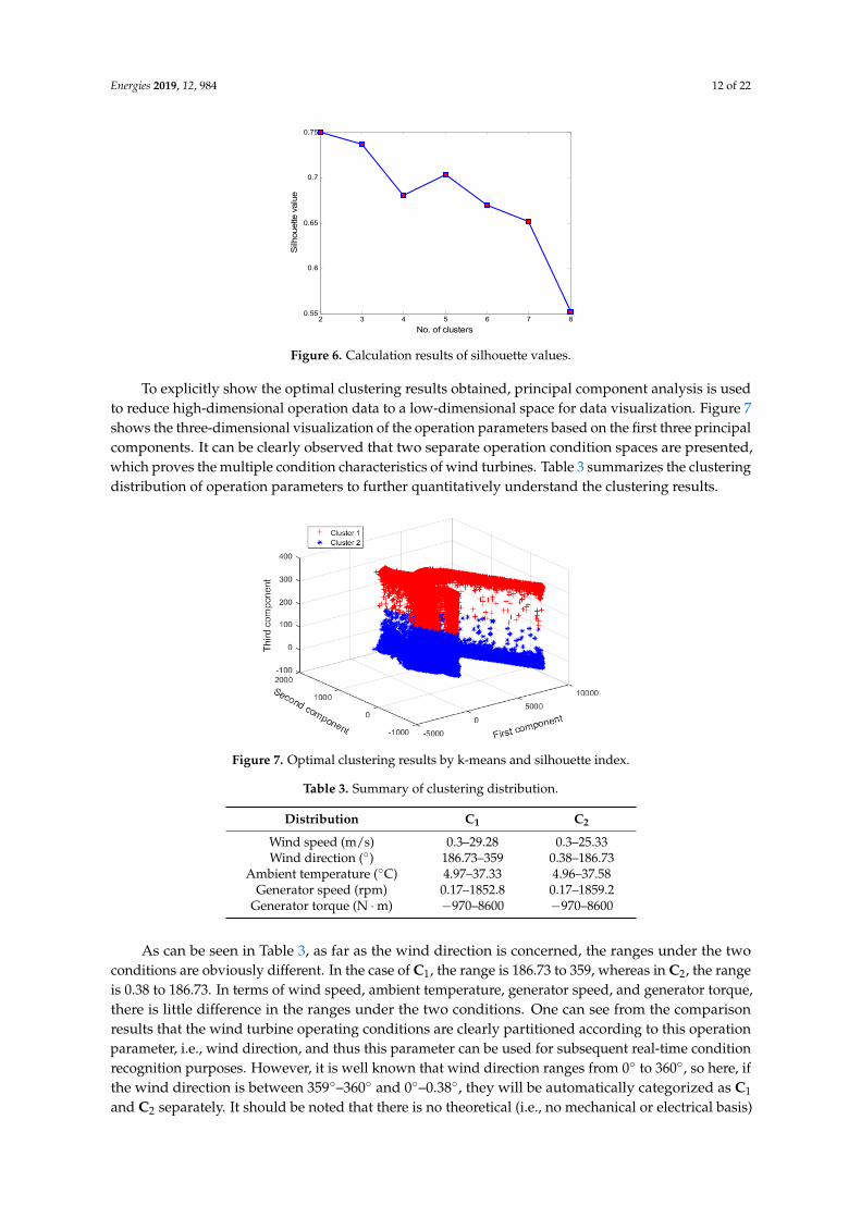
For the SCADA data from nine turbines in normal operation from 1 July to 31 August 2014,described in Section 4.1, the operation parameters representing the wind turbine operating conditionsshould first be extracted. Normally, the normalization of operation data is a basic step beforepartitioning the operating condition depending on the operation parameters to ensure the reliability ofthe clustering results. In this paper, in order to be more consistent with the operating characteristicsof wind turbines, the number of clusters is set from two to eight, and the calculation results of thesilhouette values are shown in Figure 6. From Figure 6, it can be seen that when the number ofclusters is two, the silhouette value reaches the maximum value of 0.75. This result indicates that it isoptimal to segment the wind turbine operating conditions into two sub-conditions, condition 1 (C1)and condition 2 (C2).

Energies 2019, 12, 984 12 of 22

Energies 2019, 12, 984 12 of 22

To explicitly show the optimal clustering results obtained, principal component analysis is used to reduce high-dimensional operation data to a low-dimensional space for data visualization. Figure 7 shows the three-dimensional visualization of the operation parameters based on the first three principal components. It can be clearly observed that two separate operation condition spaces are presented, which proves the multiple condition characteristics of wind turbines. Table 3 summarizes the clustering distribution of operation parameters to further quantitatively understand the clustering results.

2 3 4 5 6 7 80.55

0.6

0.65

0.7

0.75

No. of clusters

Silh

ouette

valu

e

Figure 6. Calculation results of silhouette values.

Figure 7. Optimal clustering results by k-means and silhouette index.

Table 3. Summary of clustering distribution.

Distribution C1 C2 Wind speed (m/s) 0.3–29.28 0.3–25.33 Wind direction ( °) 186.73–359 0.38–186.73 Ambient temperature ( C° ) 4.97–37.33 4.96–37.58 Generator speed (rpm) 0.17–1852.8 0.17–1859.2 Generator torque ( N m⋅ ) −970–8600 −970–8600

As can be seen in Table 3, as far as the wind direction is concerned, the ranges under the two conditions are obviously different. In the case of C1, the range is 186.73 to 359, whereas in C2, the range is 0.38 to 186.73. In terms of wind speed, ambient temperature, generator speed, and generator torque, there is little difference in the ranges under the two conditions. One can see from the comparison results that the wind turbine operating conditions are clearly partitioned according to this operation parameter, i.e., wind direction, and thus this parameter can be used for subsequent real-time condition recognition purposes. However, it is well known that wind direction ranges

Figure 6. Calculation results of silhouette values.

To explicitly show the optimal clustering results obtained, principal component analysis is usedto reduce high-dimensional operation data to a low-dimensional space for data visualization. Figure 7shows the three-dimensional visualization of the operation parameters based on the first three principalcomponents. It can be clearly observed that two separate operation condition spaces are presented,which proves the multiple condition characteristics of wind turbines. Table 3 summarizes the clusteringdistribution of operation parameters to further quantitatively understand the clustering results.

Figure 7. Optimal clustering results by k-means and silhouette index.

Table 3. Summary of clustering distribution.

Distribution C1 C2

Wind speed (m/s) 0.3–29.28 0.3–25.33Wind direction (◦) 186.73–359 0.38–186.73

Ambient temperature (◦C) 4.97–37.33 4.96–37.58Generator speed (rpm) 0.17–1852.8 0.17–1859.2

Generator torque (N ·m) −970–8600 −970–8600

As can be seen in Table 3, as far as the wind direction is concerned, the ranges under the twoconditions are obviously different. In the case of C1, the range is 186.73 to 359, whereas in C2, the rangeis 0.38 to 186.73. In terms of wind speed, ambient temperature, generator speed, and generator torque,there is little difference in the ranges under the two conditions. One can see from the comparisonresults that the wind turbine operating conditions are clearly partitioned according to this operationparameter, i.e., wind direction, and thus this parameter can be used for subsequent real-time conditionrecognition purposes. However, it is well known that wind direction ranges from 0◦ to 360◦, so here, ifthe wind direction is between 359◦–360◦ and 0◦–0.38◦, they will be automatically categorized as C1

and C2 separately. It should be noted that there is no theoretical (i.e., no mechanical or electrical basis)

Energies 2019, 12, 984 13 of 22

reasoning for the choice of wind direction as the partitioning parameter here and that this based purelyon the analysis of the clustering data.

In the following study, the original normal SCADA data from nine turbines are divided into twoportions based on the above condition partition results, and the sample numbers under C1 and C2 are154,089 and 199,042, respectively.

4.2.2. Parameter Selection for Each Condition Cluster

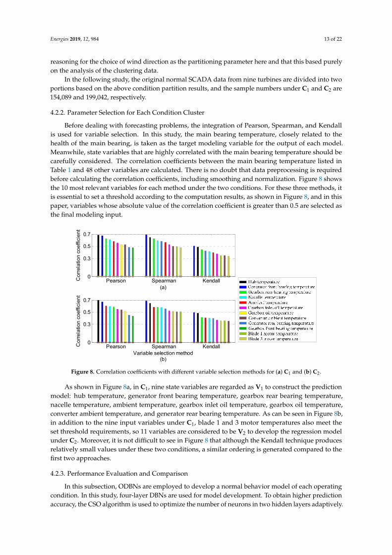
Before dealing with forecasting problems, the integration of Pearson, Spearman, and Kendallis used for variable selection. In this study, the main bearing temperature, closely related to thehealth of the main bearing, is taken as the target modeling variable for the output of each model.Meanwhile, state variables that are highly correlated with the main bearing temperature should becarefully considered. The correlation coefficients between the main bearing temperature listed inTable 1 and 48 other variables are calculated. There is no doubt that data preprocessing is requiredbefore calculating the correlation coefficients, including smoothing and normalization. Figure 8 showsthe 10 most relevant variables for each method under the two conditions. For these three methods, itis essential to set a threshold according to the computation results, as shown in Figure 8, and in thispaper, variables whose absolute value of the correlation coefficient is greater than 0.5 are selected asthe final modeling input.

Energies 2019, 12, 984 13 of 22

from 0° to 360°, so here, if the wind direction is between 359°–360° and 0°–0.38°, they will be automatically categorized as C1 and C2 separately. It should be noted that there is no theoretical (i.e., no mechanical or electrical basis) reasoning for the choice of wind direction as the partitioning parameter here and that this based purely on the analysis of the clustering data.

In the following study, the original normal SCADA data from nine turbines are divided into two portions based on the above condition partition results, and the sample numbers under C1 and C2 are 154,089 and 199,042, respectively.

4.2.2. Parameter Selection for Each Condition Cluster

Before dealing with forecasting problems, the integration of Pearson, Spearman, and Kendall is used for variable selection. In this study, the main bearing temperature, closely related to the health of the main bearing, is taken as the target modeling variable for the output of each model. Meanwhile, state variables that are highly correlated with the main bearing temperature should be carefully considered. The correlation coefficients between the main bearing temperature listed in Table 1 and 48 other variables are calculated. There is no doubt that data preprocessing is required before calculating the correlation coefficients, including smoothing and normalization. Figure 8 shows the 10 most relevant variables for each method under the two conditions. For these three methods, it is essential to set a threshold according to the computation results, as shown in Figure 8, and in this paper, variables whose absolute value of the correlation coefficient is greater than 0.5 are selected as the final modeling input.

As shown in Figure 8a, in C1, nine state variables are regarded as V1 to construct the prediction model: hub temperature, generator front bearing temperature, gearbox rear bearing temperature, nacelle temperature, ambient temperature, gearbox inlet oil temperature, gearbox oil temperature, converter ambient temperature, and generator rear bearing temperature. As can be seen in Figure 8b, in addition to the nine input variables under C1, blade 1 and 3 motor temperatures also meet the set threshold requirements, so 11 variables are considered to be V2 to develop the regression model under C2. Moreover, it is not difficult to see in Figure 8 that although the Kendall technique produces relatively small values under these two conditions, a similar ordering is generated compared to the first two approaches.

Pearson Spearman Kendall0

0.3

0.5

0.7

(a)

Co

rre

latio

n c

oe

ffici

en

t

Pearson Spearman Kendall0

0.3

0.5

0.7

Co

rre

latio

n c

oe

ffici

en

t

Variable selection method(b)

Figure 8. Correlation coefficients with different variable selection methods for (a) C1 and (b) C2.

4.2.3. Performance Evaluation and Comparison

In this subsection, ODBNs are employed to develop a normal behavior model of each operating condition. In this study, four-layer DBNs are used for model development. To obtain higher prediction accuracy, the CSO algorithm is used to optimize the number of neurons in two

Figure 8. Correlation coefficients with different variable selection methods for (a) C1 and (b) C2.

As shown in Figure 8a, in C1, nine state variables are regarded as V1 to construct the predictionmodel: hub temperature, generator front bearing temperature, gearbox rear bearing temperature,nacelle temperature, ambient temperature, gearbox inlet oil temperature, gearbox oil temperature,converter ambient temperature, and generator rear bearing temperature. As can be seen in Figure 8b,in addition to the nine input variables under C1, blade 1 and 3 motor temperatures also meet theset threshold requirements, so 11 variables are considered to be V2 to develop the regression modelunder C2. Moreover, it is not difficult to see in Figure 8 that although the Kendall technique producesrelatively small values under these two conditions, a similar ordering is generated compared to thefirst two approaches.

4.2.3. Performance Evaluation and Comparison

In this subsection, ODBNs are employed to develop a normal behavior model of each operatingcondition. In this study, four-layer DBNs are used for model development. To obtain higher predictionaccuracy, the CSO algorithm is used to optimize the number of neurons in two hidden layers adaptively.

Energies 2019, 12, 984 14 of 22

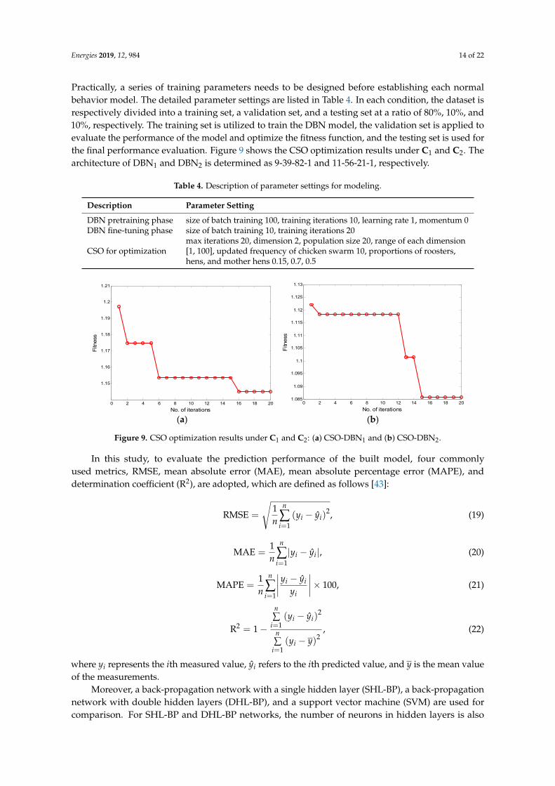
Practically, a series of training parameters needs to be designed before establishing each normalbehavior model. The detailed parameter settings are listed in Table 4. In each condition, the dataset isrespectively divided into a training set, a validation set, and a testing set at a ratio of 80%, 10%, and10%, respectively. The training set is utilized to train the DBN model, the validation set is applied toevaluate the performance of the model and optimize the fitness function, and the testing set is used forthe final performance evaluation. Figure 9 shows the CSO optimization results under C1 and C2. Thearchitecture of DBN1 and DBN2 is determined as 9-39-82-1 and 11-56-21-1, respectively.

Table 4. Description of parameter settings for modeling.

Description Parameter Setting

DBN pretraining phase size of batch training 100, training iterations 10, learning rate 1, momentum 0DBN fine-tuning phase size of batch training 10, training iterations 20

CSO for optimizationmax iterations 20, dimension 2, population size 20, range of each dimension[1, 100], updated frequency of chicken swarm 10, proportions of roosters,hens, and mother hens 0.15, 0.7, 0.5

Energies 2019, 12, 984 14 of 22

hidden layers adaptively. Practically, a series of training parameters needs to be designed before establishing each normal behavior model. The detailed parameter settings are listed in Table 4. In each condition, the dataset is respectively divided into a training set, a validation set, and a testing set at a ratio of 80%, 10%, and 10%, respectively. The training set is utilized to train the DBN model, the validation set is applied to evaluate the performance of the model and optimize the fitness function, and the testing set is used for the final performance evaluation. Figure 9 shows the CSO optimization results under C1 and C2. The architecture of DBN1 and DBN2 is determined as 9-39-82-1 and 11-56-21-1, respectively.

Table 4. Description of parameter settings for modeling.

Description Parameter Setting DBN pretraining phase size of batch training 100, training iterations 10, learning rate 1, momentum 0

DBN fine-tuning phase

size of batch training 10, training iterations 20

CSO for optimization

max iterations 20, dimension 2, population size 20, range of each dimension [1, 100], updated frequency of chicken swarm 10, proportions of roosters, hens, and mother hens 0.15, 0.7, 0.5

0 2 4 6 8 10 12 14 16 18 20

1.15

1.16

1.17

1.18

1.19

1.2

1.21

No. of iterations

Fitn

ess

(a)

0 2 4 6 8 10 12 14 16 18 201.085

1.09

1.095

1.1

1.105

1.11

1.115

1.12

1.125

1.13

No. of iterations

Fitn

ess

(b) Figure 9. CSO optimization results under C1 and C2: (a) CSO-DBN1 and (b) CSO-DBN2.

In this study, to evaluate the prediction performance of the built model, four commonly used metrics, RMSE, mean absolute error (MAE), mean absolute percentage error (MAPE), and determination coefficient (R2), are adopted, which are defined as follows [43]:

2

1

1 ˆRMSE ( )n

i iiy y

n =

= − ,

(19)

1

1 ˆMAEn

i iiy y

n =

= − ,

(20)

1

ˆ1MAPE 100n

i i

i i

y yn y=

−= × ,

(21)

2

2 1

2

1

ˆ( )R 1

( )

n

i iin

ii

y y

y y

=

=

−= −

−

,

(22)

where iy represents the thi measured value, ˆiy refers to the thi predicted value, and y is the mean value of the measurements.

Figure 9. CSO optimization results under C1 and C2: (a) CSO-DBN1 and (b) CSO-DBN2.

In this study, to evaluate the prediction performance of the built model, four commonlyused metrics, RMSE, mean absolute error (MAE), mean absolute percentage error (MAPE), anddetermination coefficient (R2), are adopted, which are defined as follows [43]:

RMSE =

√1n

n

∑i=1

(yi − yi)2, (19)

MAE =1n

n

∑i=1|yi − yi|, (20)

MAPE =1n

n

∑i=1

∣∣∣∣yi − yiyi

∣∣∣∣× 100, (21)

R2 = 1−

n∑

i=1(yi − yi)

2

n∑

i=1(yi − y)2

, (22)

where yi represents the ith measured value, yi refers to the ith predicted value, and y is the mean valueof the measurements.

Moreover, a back-propagation network with a single hidden layer (SHL-BP), a back-propagationnetwork with double hidden layers (DHL-BP), and a support vector machine (SVM) are used forcomparison. For SHL-BP and DHL-BP networks, the number of neurons in hidden layers is also

Energies 2019, 12, 984 15 of 22

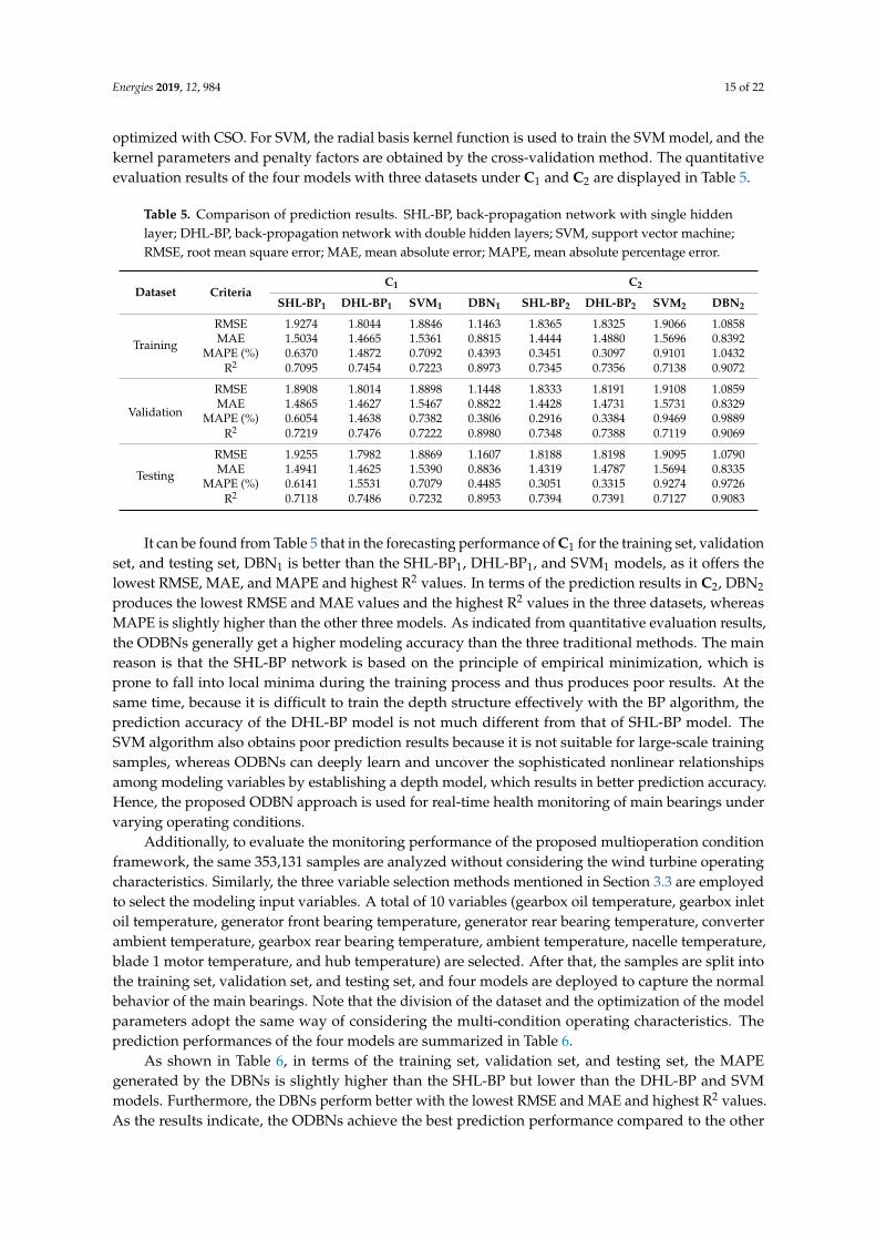
optimized with CSO. For SVM, the radial basis kernel function is used to train the SVM model, and thekernel parameters and penalty factors are obtained by the cross-validation method. The quantitativeevaluation results of the four models with three datasets under C1 and C2 are displayed in Table 5.

Table 5. Comparison of prediction results. SHL-BP, back-propagation network with single hiddenlayer; DHL-BP, back-propagation network with double hidden layers; SVM, support vector machine;RMSE, root mean square error; MAE, mean absolute error; MAPE, mean absolute percentage error.

Dataset CriteriaC1 C2

SHL-BP1 DHL-BP1 SVM1 DBN1 SHL-BP2 DHL-BP2 SVM2 DBN2

Training

RMSE 1.9274 1.8044 1.8846 1.1463 1.8365 1.8325 1.9066 1.0858MAE 1.5034 1.4665 1.5361 0.8815 1.4444 1.4880 1.5696 0.8392

MAPE (%) 0.6370 1.4872 0.7092 0.4393 0.3451 0.3097 0.9101 1.0432R2 0.7095 0.7454 0.7223 0.8973 0.7345 0.7356 0.7138 0.9072

Validation

RMSE 1.8908 1.8014 1.8898 1.1448 1.8333 1.8191 1.9108 1.0859MAE 1.4865 1.4627 1.5467 0.8822 1.4428 1.4731 1.5731 0.8329

MAPE (%) 0.6054 1.4638 0.7382 0.3806 0.2916 0.3384 0.9469 0.9889R2 0.7219 0.7476 0.7222 0.8980 0.7348 0.7388 0.7119 0.9069

Testing

RMSE 1.9255 1.7982 1.8869 1.1607 1.8188 1.8198 1.9095 1.0790MAE 1.4941 1.4625 1.5390 0.8836 1.4319 1.4787 1.5694 0.8335

MAPE (%) 0.6141 1.5531 0.7079 0.4485 0.3051 0.3315 0.9274 0.9726R2 0.7118 0.7486 0.7232 0.8953 0.7394 0.7391 0.7127 0.9083

It can be found from Table 5 that in the forecasting performance of C1 for the training set, validationset, and testing set, DBN1 is better than the SHL-BP1, DHL-BP1, and SVM1 models, as it offers thelowest RMSE, MAE, and MAPE and highest R2 values. In terms of the prediction results in C2, DBN2

produces the lowest RMSE and MAE values and the highest R2 values in the three datasets, whereasMAPE is slightly higher than the other three models. As indicated from quantitative evaluation results,the ODBNs generally get a higher modeling accuracy than the three traditional methods. The mainreason is that the SHL-BP network is based on the principle of empirical minimization, which isprone to fall into local minima during the training process and thus produces poor results. At thesame time, because it is difficult to train the depth structure effectively with the BP algorithm, theprediction accuracy of the DHL-BP model is not much different from that of SHL-BP model. TheSVM algorithm also obtains poor prediction results because it is not suitable for large-scale trainingsamples, whereas ODBNs can deeply learn and uncover the sophisticated nonlinear relationshipsamong modeling variables by establishing a depth model, which results in better prediction accuracy.Hence, the proposed ODBN approach is used for real-time health monitoring of main bearings undervarying operating conditions.

Additionally, to evaluate the monitoring performance of the proposed multioperation conditionframework, the same 353,131 samples are analyzed without considering the wind turbine operatingcharacteristics. Similarly, the three variable selection methods mentioned in Section 3.3 are employedto select the modeling input variables. A total of 10 variables (gearbox oil temperature, gearbox inletoil temperature, generator front bearing temperature, generator rear bearing temperature, converterambient temperature, gearbox rear bearing temperature, ambient temperature, nacelle temperature,blade 1 motor temperature, and hub temperature) are selected. After that, the samples are split intothe training set, validation set, and testing set, and four models are deployed to capture the normalbehavior of the main bearings. Note that the division of the dataset and the optimization of the modelparameters adopt the same way of considering the multi-condition operating characteristics. Theprediction performances of the four models are summarized in Table 6.

As shown in Table 6, in terms of the training set, validation set, and testing set, the MAPEgenerated by the DBNs is slightly higher than the SHL-BP but lower than the DHL-BP and SVMmodels. Furthermore, the DBNs perform better with the lowest RMSE and MAE and highest R2 values.As the results indicate, the ODBNs achieve the best prediction performance compared to the other

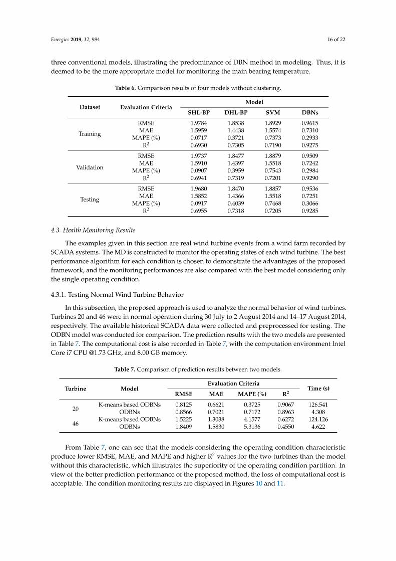
Energies 2019, 12, 984 16 of 22

three conventional models, illustrating the predominance of DBN method in modeling. Thus, it isdeemed to be the more appropriate model for monitoring the main bearing temperature.

Table 6. Comparison results of four models without clustering.

Dataset Evaluation CriteriaModel

SHL-BP DHL-BP SVM DBNs

Training

RMSE 1.9784 1.8538 1.8929 0.9615MAE 1.5959 1.4438 1.5574 0.7310

MAPE (%) 0.0717 0.3721 0.7373 0.2933R2 0.6930 0.7305 0.7190 0.9275

Validation

RMSE 1.9737 1.8477 1.8879 0.9509MAE 1.5910 1.4397 1.5518 0.7242

MAPE (%) 0.0907 0.3959 0.7543 0.2984R2 0.6941 0.7319 0.7201 0.9290

Testing

RMSE 1.9680 1.8470 1.8857 0.9536MAE 1.5852 1.4366 1.5518 0.7251

MAPE (%) 0.0917 0.4039 0.7468 0.3066R2 0.6955 0.7318 0.7205 0.9285

4.3. Health Monitoring Results

The examples given in this section are real wind turbine events from a wind farm recorded bySCADA systems. The MD is constructed to monitor the operating states of each wind turbine. The bestperformance algorithm for each condition is chosen to demonstrate the advantages of the proposedframework, and the monitoring performances are also compared with the best model considering onlythe single operating condition.

4.3.1. Testing Normal Wind Turbine Behavior

In this subsection, the proposed approach is used to analyze the normal behavior of wind turbines.Turbines 20 and 46 were in normal operation during 30 July to 2 August 2014 and 14–17 August 2014,respectively. The available historical SCADA data were collected and preprocessed for testing. TheODBN model was conducted for comparison. The prediction results with the two models are presentedin Table 7. The computational cost is also recorded in Table 7, with the computation environment IntelCore i7 CPU @1.73 GHz, and 8.00 GB memory.

Table 7. Comparison of prediction results between two models.

Turbine ModelEvaluation Criteria

Time (s)RMSE MAE MAPE (%) R2

20K-means based ODBNs 0.8125 0.6621 0.3725 0.9067 126.541

ODBNs 0.8566 0.7021 0.7172 0.8963 4.308

46K-means based ODBNs 1.5225 1.3038 4.1577 0.6272 124.126

ODBNs 1.8409 1.5830 5.3136 0.4550 4.622

From Table 7, one can see that the models considering the operating condition characteristicproduce lower RMSE, MAE, and MAPE and higher R2 values for the two turbines than the modelwithout this characteristic, which illustrates the superiority of the operating condition partition. Inview of the better prediction performance of the proposed method, the loss of computational cost isacceptable. The condition monitoring results are displayed in Figures 10 and 11.

Energies 2019, 12, 984 17 of 22Energies 2019, 12, 984 17 of 22

1000 2000 3000 4000 5000 6000 7000 8000 9000 10000 110000

0.5

1

1.5

2

2.5

3

3.5

4

4.5

5

No. of samples

Mahal

anobis

dis

tance

Mahalanobis distance

Threshold

1000 2000 3000 4000 5000 6000 7000 8000 9000 10000 110000

0.5

1

1.5

2

2.5

3

3.5

4

4.5

5

No. of samples

Mahala

nobis

dis

tance

Mahalanobis distance

Threshold

Figure 10. Condition monitoring results for Turbine 20: (a) K-means–based ODBNs and (b) ODBNs.

1000 2000 3000 4000 5000 6000 7000 8000 9000 10000 110000

0.5

1

1.5

2

2.5

3

3.5

4

4.5

5

No. of samples

Maha

lano

bis

dis

tance

Mahalanobis distance

Threshold

1000 2000 3000 4000 5000 6000 7000 8000 9000 10000 110000

0.5

1

1.5

2

2.5

3

3.5

4

4.5

5

No. of samples

Mahala

nobis

dis

tance

Mahalanobis distance

Threshold

Figure 11. Condition monitoring results for Turbine 46: (a) K-means based ODBNs and (b) ODBNs.

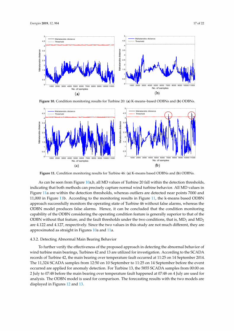
As can be seen from Figures 10a,b, all MD values of Turbine 20 fall within the detection thresholds, indicating that both methods can precisely capture normal wind turbine behavior. All MD values in Figure 11a are within the detection thresholds, whereas outliers are detected near points 7000 and 11,000 in Figure 11b. According to the monitoring results in Figure 11, the k-means based ODBN approach successfully monitors the operating state of Turbine 46 without false alarms, whereas the ODBN model produces false alarms. Hence, it can be concluded that the condition monitoring capability of the ODBN considering the operating condition feature is generally superior to that of the ODBN without that feature, and the fault thresholds under the two conditions, that is, MD1 and MD2 are 4.122 and 4.127, respectively. Since the two values in this study are not much different, they are approximated as straight in Figures 10a and 11a.

4.3.2. Detecting Abnormal Main Bearing Behavior

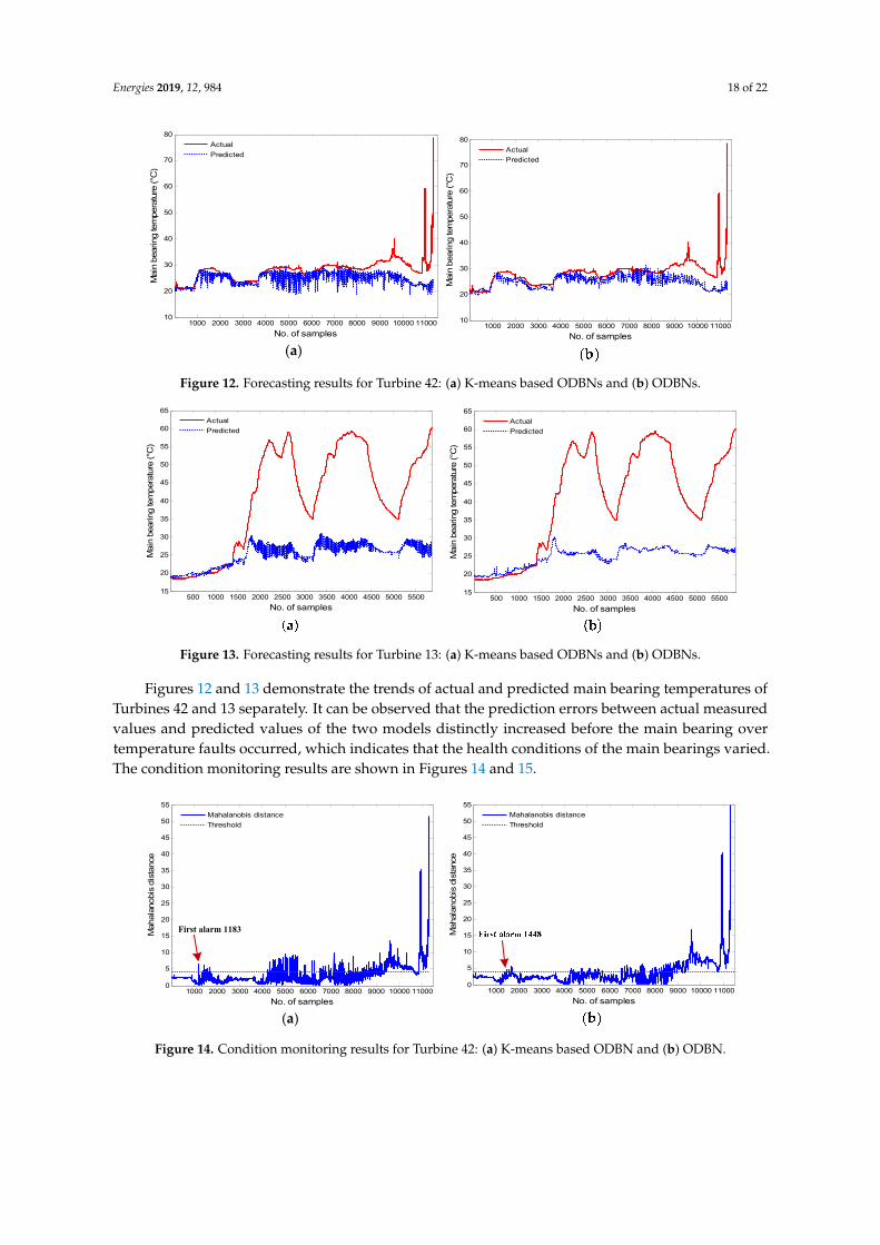
To further verify the effectiveness of the proposed approach in detecting the abnormal behavior of wind turbine main bearings, Turbines 42 and 13 are utilized for investigation. According to the SCADA records of Turbine 42, the main bearing over temperature fault occurred at 11:25 on 14 September 2014. The 11,324 SCADA samples from 12:50 on 10 September to 11:25 on 14 September before the event occurred are applied for anomaly detection. For Turbine 13, the 5855 SCADA samples from 00:00 on 2 July to 07:48 before the main bearing over temperature fault happened at 07:48 on 4 July are used for analysis. The ODBN model is used for comparison. The forecasting results with the two models are displayed in Figures 12 and 13.

Figures 12 and 13 demonstrate the trends of actual and predicted main bearing temperatures of Turbines 42 and 13 separately. It can be observed that the prediction errors between actual measured values and predicted values of the two models distinctly increased before the main

Figure 10. Condition monitoring results for Turbine 20: (a) K-means–based ODBNs and (b) ODBNs.

Energies 2019, 12, 984 17 of 22

1000 2000 3000 4000 5000 6000 7000 8000 9000 10000 110000

0.5

1

1.5

2

2.5

3

3.5

4

4.5

5

No. of samples

Mahal

anobis

dis

tance

Mahalanobis distance

Threshold

1000 2000 3000 4000 5000 6000 7000 8000 9000 10000 110000

0.5

1

1.5

2

2.5

3

3.5

4

4.5

5

No. of samples

Mahala

nobis

dis

tance

Mahalanobis distance

Threshold

Figure 10. Condition monitoring results for Turbine 20: (a) K-means–based ODBNs and (b) ODBNs.

1000 2000 3000 4000 5000 6000 7000 8000 9000 10000 110000

0.5

1

1.5

2

2.5

3

3.5

4

4.5

5

No. of samples

Maha

lano

bis

dis

tance

Mahalanobis distance

Threshold

1000 2000 3000 4000 5000 6000 7000 8000 9000 10000 110000

0.5

1

1.5

2

2.5

3

3.5

4

4.5

5

No. of samples

Mahala

nobis

dis

tance

Mahalanobis distance

Threshold

Figure 11. Condition monitoring results for Turbine 46: (a) K-means based ODBNs and (b) ODBNs.

As can be seen from Figures 10a,b, all MD values of Turbine 20 fall within the detection thresholds, indicating that both methods can precisely capture normal wind turbine behavior. All MD values in Figure 11a are within the detection thresholds, whereas outliers are detected near points 7000 and 11,000 in Figure 11b. According to the monitoring results in Figure 11, the k-means based ODBN approach successfully monitors the operating state of Turbine 46 without false alarms, whereas the ODBN model produces false alarms. Hence, it can be concluded that the condition monitoring capability of the ODBN considering the operating condition feature is generally superior to that of the ODBN without that feature, and the fault thresholds under the two conditions, that is, MD1 and MD2 are 4.122 and 4.127, respectively. Since the two values in this study are not much different, they are approximated as straight in Figures 10a and 11a.

4.3.2. Detecting Abnormal Main Bearing Behavior

To further verify the effectiveness of the proposed approach in detecting the abnormal behavior of wind turbine main bearings, Turbines 42 and 13 are utilized for investigation. According to the SCADA records of Turbine 42, the main bearing over temperature fault occurred at 11:25 on 14 September 2014. The 11,324 SCADA samples from 12:50 on 10 September to 11:25 on 14 September before the event occurred are applied for anomaly detection. For Turbine 13, the 5855 SCADA samples from 00:00 on 2 July to 07:48 before the main bearing over temperature fault happened at 07:48 on 4 July are used for analysis. The ODBN model is used for comparison. The forecasting results with the two models are displayed in Figures 12 and 13.

Figures 12 and 13 demonstrate the trends of actual and predicted main bearing temperatures of Turbines 42 and 13 separately. It can be observed that the prediction errors between actual measured values and predicted values of the two models distinctly increased before the main

Figure 11. Condition monitoring results for Turbine 46: (a) K-means based ODBNs and (b) ODBNs.

As can be seen from Figure 10a,b, all MD values of Turbine 20 fall within the detection thresholds,indicating that both methods can precisely capture normal wind turbine behavior. All MD values inFigure 11a are within the detection thresholds, whereas outliers are detected near points 7000 and11,000 in Figure 11b. According to the monitoring results in Figure 11, the k-means based ODBNapproach successfully monitors the operating state of Turbine 46 without false alarms, whereas theODBN model produces false alarms. Hence, it can be concluded that the condition monitoringcapability of the ODBN considering the operating condition feature is generally superior to that of theODBN without that feature, and the fault thresholds under the two conditions, that is, MD1 and MD2

are 4.122 and 4.127, respectively. Since the two values in this study are not much different, they areapproximated as straight in Figures 10a and 11a.

4.3.2. Detecting Abnormal Main Bearing Behavior

To further verify the effectiveness of the proposed approach in detecting the abnormal behavior ofwind turbine main bearings, Turbines 42 and 13 are utilized for investigation. According to the SCADArecords of Turbine 42, the main bearing over temperature fault occurred at 11:25 on 14 September 2014.The 11,324 SCADA samples from 12:50 on 10 September to 11:25 on 14 September before the eventoccurred are applied for anomaly detection. For Turbine 13, the 5855 SCADA samples from 00:00 on2 July to 07:48 before the main bearing over temperature fault happened at 07:48 on 4 July are used foranalysis. The ODBN model is used for comparison. The forecasting results with the two models aredisplayed in Figures 12 and 13.

Energies 2019, 12, 984 18 of 22

Energies 2019, 12, 984 18 of 22

bearing over temperature faults occurred, which indicates that the health conditions of the main bearings varied. The condition monitoring results are shown in Figures 14 and 15.

1000 2000 3000 4000 5000 6000 7000 8000 9000 10000 1100010

20

30

40

50

60

70

80

No. of samples

Main

bearing te

mpera

ture

(°C

)

Actual

Predicted

(a)

1000 2000 3000 4000 5000 6000 7000 8000 9000 10000 1100010

20

30

40

50

60

70

80

No. of samples

Mai

n bea

ring

tem

per

atu

re (°C

)

Actual

Predicted

Figure 12. Forecasting results for Turbine 42: (a) K-means based ODBNs and (b) ODBNs.

500 1000 1500 2000 2500 3000 3500 4000 4500 5000 550015

20

25

30

35

40

45

50

55

60

65

No. of samples

Mai

n b

ear

ing te

mper

atu

re (°C

)

Actual

Predicted

500 1000 1500 2000 2500 3000 3500 4000 4500 5000 550015

20

25

30

35

40

45

50

55

60

65

No. of samples

Main

bearin

g te

mper

atu

re (°C

)

Actual

Predicted

Figure 13. Forecasting results for Turbine 13: (a) K-means based ODBNs and (b) ODBNs.

Figure 14a displays the monitoring results of the proposed framework for Turbine 42, while Figure 14b illustrates the monitoring results of the ODBN model in the same turbine. As shown in Figure 14a, the MD value first crosses the fault threshold at sample point 1183, and an incipient main bearing fault is detected. However, the actual fault occurred at 11:25 on 14 September 2014, which is the 11,325th sample point. Each sample point is separated by an interval of 30 s, so the k-means based ODBN approach can detect the main bearing fault approximately 84.5 h in advance. As can be seen from Figure 14b, the MD value first exceeds the threshold at sample point 1448, and an early alarm is signaled, thus predicting the over temperature event almost 82.3 h ahead of the actual fault. From the computation results in Figure 14, both models can identify the upcoming main bearing fault successfully. Nevertheless, the proposed k-means based ODBN model is able to detect the anomaly of the main bearing nearly 2.2 h earlier than the ODBN approach. At the same time, it also means that there is only a 2.2 h improvement in using the k-means based ODBN model over the ODBN model (82.3 vs. 84.5 h), which represents only a 2.6% improvement. Still, this can also provide more time for wind farm operators to take appropriate measures. If the abnormal main bearing can be repaired and replaced in time, possible major accidents and unnecessary maintenance costs and downtime can be avoided. The computational time of k-means based ODBN and ODBN methods during the condition monitoring is 129.596 s and 4.748 s, respectively.

Figures 15a,b plot the monitoring results of the k-means–based ODBN and ODBN models, respectively, for Turbine 13. From Figure 15a, one can see that based on the fault thresholds, the alarm is first issued at sample point 1457, while the actual fault happened at 07:48 on 4 July 2014, which is the 5856th sample point. Therefore, the proposed approach can detect the fault almost 36.6

Figure 12. Forecasting results for Turbine 42: (a) K-means based ODBNs and (b) ODBNs.

Energies 2019, 12, 984 18 of 22

bearing over temperature faults occurred, which indicates that the health conditions of the main bearings varied. The condition monitoring results are shown in Figures 14 and 15.

1000 2000 3000 4000 5000 6000 7000 8000 9000 10000 1100010

20

30

40

50

60

70

80

No. of samples

Main

bearing te

mpera

ture

(°C

)

Actual

Predicted

(a)

1000 2000 3000 4000 5000 6000 7000 8000 9000 10000 1100010

20

30

40

50

60

70

80

No. of samples

Mai

n bea

ring

tem

per

atu

re (°C

)

Actual

Predicted

Figure 12. Forecasting results for Turbine 42: (a) K-means based ODBNs and (b) ODBNs.

500 1000 1500 2000 2500 3000 3500 4000 4500 5000 550015

20

25

30

35

40

45

50

55

60

65

No. of samples

Mai

n b

ear

ing te

mper

atu

re (°C

)

Actual

Predicted

500 1000 1500 2000 2500 3000 3500 4000 4500 5000 550015

20

25

30

35

40

45

50

55

60

65

No. of samples

Main

bearin

g te

mper

atu

re (°C

)

Actual

Predicted

Figure 13. Forecasting results for Turbine 13: (a) K-means based ODBNs and (b) ODBNs.

Figure 14a displays the monitoring results of the proposed framework for Turbine 42, while Figure 14b illustrates the monitoring results of the ODBN model in the same turbine. As shown in Figure 14a, the MD value first crosses the fault threshold at sample point 1183, and an incipient main bearing fault is detected. However, the actual fault occurred at 11:25 on 14 September 2014, which is the 11,325th sample point. Each sample point is separated by an interval of 30 s, so the k-means based ODBN approach can detect the main bearing fault approximately 84.5 h in advance. As can be seen from Figure 14b, the MD value first exceeds the threshold at sample point 1448, and an early alarm is signaled, thus predicting the over temperature event almost 82.3 h ahead of the actual fault. From the computation results in Figure 14, both models can identify the upcoming main bearing fault successfully. Nevertheless, the proposed k-means based ODBN model is able to detect the anomaly of the main bearing nearly 2.2 h earlier than the ODBN approach. At the same time, it also means that there is only a 2.2 h improvement in using the k-means based ODBN model over the ODBN model (82.3 vs. 84.5 h), which represents only a 2.6% improvement. Still, this can also provide more time for wind farm operators to take appropriate measures. If the abnormal main bearing can be repaired and replaced in time, possible major accidents and unnecessary maintenance costs and downtime can be avoided. The computational time of k-means based ODBN and ODBN methods during the condition monitoring is 129.596 s and 4.748 s, respectively.

Figures 15a,b plot the monitoring results of the k-means–based ODBN and ODBN models, respectively, for Turbine 13. From Figure 15a, one can see that based on the fault thresholds, the alarm is first issued at sample point 1457, while the actual fault happened at 07:48 on 4 July 2014, which is the 5856th sample point. Therefore, the proposed approach can detect the fault almost 36.6

Figure 13. Forecasting results for Turbine 13: (a) K-means based ODBNs and (b) ODBNs.

Figures 12 and 13 demonstrate the trends of actual and predicted main bearing temperatures ofTurbines 42 and 13 separately. It can be observed that the prediction errors between actual measuredvalues and predicted values of the two models distinctly increased before the main bearing overtemperature faults occurred, which indicates that the health conditions of the main bearings varied.The condition monitoring results are shown in Figures 14 and 15.

Energies 2019, 12, 984 19 of 22

h in advance. As shown in Figure 15b, the MD value also first crosses the fault threshold at point 1457, and an early alarm is triggered. According to the computation results in Figure 15, one can conclude that the two models are able to simultaneously identify the anomaly of the main bearing nearly 36.6 h in advance, and the computational time of k-means-based ODBN and ODBN methods during the condition monitoring is 2.567 s and 68.046 s, respectively.

1000 2000 3000 4000 5000 6000 7000 8000 9000 10000 110000

5

10

15

20

25

30

35

40

45

50

55

No. of samples

Maha

lanob

is d

ista

nce

Mahalanobis distance

Threshold

First alarm 1183

(a)

1000 2000 3000 4000 5000 6000 7000 8000 9000 10000 110000

5

10

15

20

25

30

35

40

45

50

55

No. of samples

Mahala

nobis

dis

tance

Mahalanobis distance

Threshold

Figure 14. Condition monitoring results for Turbine 42: (a) K-means based ODBN and (b) ODBN.

500 1000 1500 2000 2500 3000 3500 4000 4500 5000 55000

5

10

15

20

25

30

35

40

No. of samples

Mahal

anob

is d

ista

nce

Mahalanobis distance

Threshold

500 1000 1500 2000 2500 3000 3500 4000 4500 5000 55000

5

10

15

20

25

30

35

40

No. of samples

Mahala

nobis

dis

tance

Mahalanobis distance

Threshold

First alarm 1457

(b) Figure 15. Condition monitoring results for Turbine 13: (a) K-means based ODBN and (b) ODBN.

Based on the application analysis of the above real case, the proposed framework has certain advantages in the real-time health monitoring of wind turbines, which can mainly be attributed to the integration of multioperation condition monitoring and deep feature characterization. Meanwhile, the computational time is relatively high due to the complex procedures of the proposed divide-and-conquer strategy, but within acceptable limits. It is worth noting that the study is limited by the use of only three months of SCADA data and that the results are not valid for longer time periods.

5. Conclusions

A health monitoring method for wind turbine operational states has been proposed to consider the dynamic operating conditions of wind turbines and address the difficulty in accurately building normal behavior models. In the proposed approach, on the one hand, considering the multiple operating characteristics of wind turbines, a general multioperation condition partition scheme based on the k-means clustering method was utilized to segment the whole operation into multiple sub-operation conditions. One the other hand, ODBNs were applied to construct a healthy prediction model in each condition cluster where model parameters are optimally selected by the CSO algorithm. Compared with the conventional back-propagation and support vector machine

Figure 14. Condition monitoring results for Turbine 42: (a) K-means based ODBN and (b) ODBN.

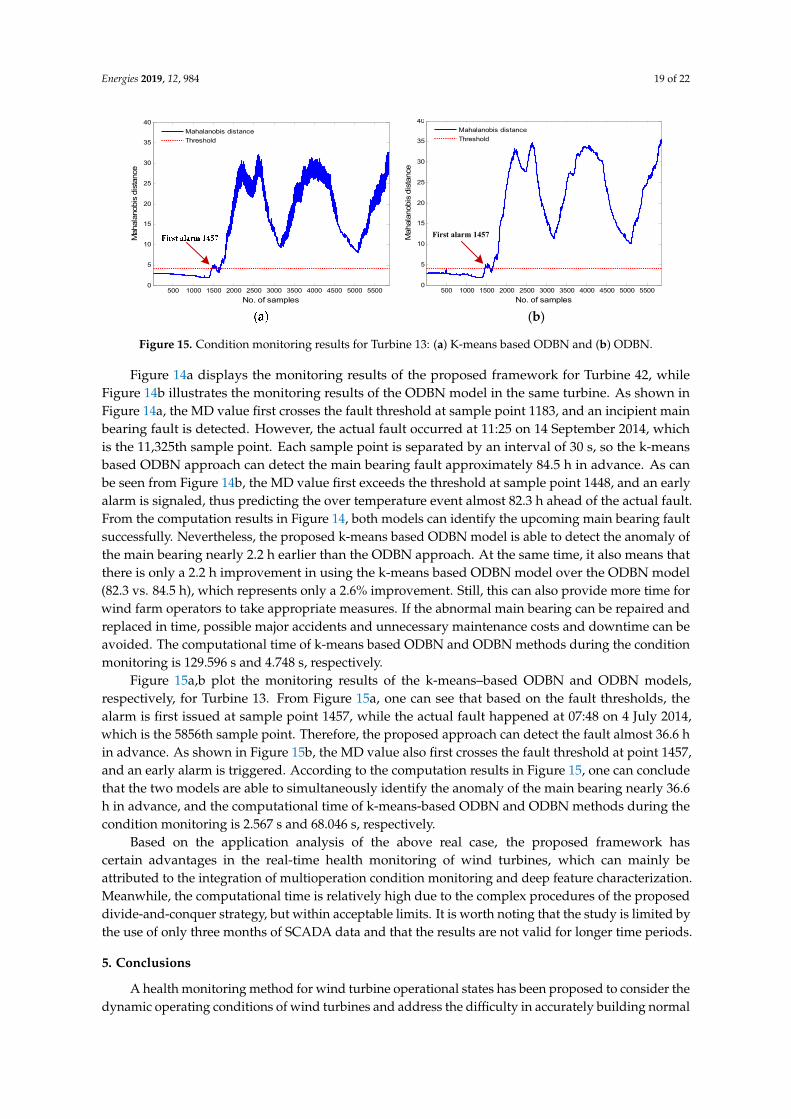
Energies 2019, 12, 984 19 of 22

Energies 2019, 12, 984 19 of 22

h in advance. As shown in Figure 15b, the MD value also first crosses the fault threshold at point 1457, and an early alarm is triggered. According to the computation results in Figure 15, one can conclude that the two models are able to simultaneously identify the anomaly of the main bearing nearly 36.6 h in advance, and the computational time of k-means-based ODBN and ODBN methods during the condition monitoring is 2.567 s and 68.046 s, respectively.

1000 2000 3000 4000 5000 6000 7000 8000 9000 10000 110000

5

10

15

20

25

30

35

40

45

50

55

No. of samples

Maha

lanob

is d

ista

nce

Mahalanobis distance

Threshold

First alarm 1183

(a)

1000 2000 3000 4000 5000 6000 7000 8000 9000 10000 110000

5

10

15

20

25

30

35

40

45

50

55

No. of samples

Mahala

nobis

dis

tance

Mahalanobis distance

Threshold

Figure 14. Condition monitoring results for Turbine 42: (a) K-means based ODBN and (b) ODBN.

500 1000 1500 2000 2500 3000 3500 4000 4500 5000 55000

5

10

15

20

25

30

35

40

No. of samples

Mahal

anob

is d

ista

nce

Mahalanobis distance

Threshold

500 1000 1500 2000 2500 3000 3500 4000 4500 5000 55000

5

10

15

20

25

30

35

40

No. of samples

Mahala

nobis

dis

tance

Mahalanobis distance

Threshold

First alarm 1457

(b) Figure 15. Condition monitoring results for Turbine 13: (a) K-means based ODBN and (b) ODBN.

Based on the application analysis of the above real case, the proposed framework has certain advantages in the real-time health monitoring of wind turbines, which can mainly be attributed to the integration of multioperation condition monitoring and deep feature characterization. Meanwhile, the computational time is relatively high due to the complex procedures of the proposed divide-and-conquer strategy, but within acceptable limits. It is worth noting that the study is limited by the use of only three months of SCADA data and that the results are not valid for longer time periods.

5. Conclusions

A health monitoring method for wind turbine operational states has been proposed to consider the dynamic operating conditions of wind turbines and address the difficulty in accurately building normal behavior models. In the proposed approach, on the one hand, considering the multiple operating characteristics of wind turbines, a general multioperation condition partition scheme based on the k-means clustering method was utilized to segment the whole operation into multiple sub-operation conditions. One the other hand, ODBNs were applied to construct a healthy prediction model in each condition cluster where model parameters are optimally selected by the CSO algorithm. Compared with the conventional back-propagation and support vector machine

Figure 15. Condition monitoring results for Turbine 13: (a) K-means based ODBN and (b) ODBN.

Figure 14a displays the monitoring results of the proposed framework for Turbine 42, whileFigure 14b illustrates the monitoring results of the ODBN model in the same turbine. As shown inFigure 14a, the MD value first crosses the fault threshold at sample point 1183, and an incipient mainbearing fault is detected. However, the actual fault occurred at 11:25 on 14 September 2014, whichis the 11,325th sample point. Each sample point is separated by an interval of 30 s, so the k-meansbased ODBN approach can detect the main bearing fault approximately 84.5 h in advance. As canbe seen from Figure 14b, the MD value first exceeds the threshold at sample point 1448, and an earlyalarm is signaled, thus predicting the over temperature event almost 82.3 h ahead of the actual fault.From the computation results in Figure 14, both models can identify the upcoming main bearing faultsuccessfully. Nevertheless, the proposed k-means based ODBN model is able to detect the anomaly ofthe main bearing nearly 2.2 h earlier than the ODBN approach. At the same time, it also means thatthere is only a 2.2 h improvement in using the k-means based ODBN model over the ODBN model(82.3 vs. 84.5 h), which represents only a 2.6% improvement. Still, this can also provide more time forwind farm operators to take appropriate measures. If the abnormal main bearing can be repaired andreplaced in time, possible major accidents and unnecessary maintenance costs and downtime can beavoided. The computational time of k-means based ODBN and ODBN methods during the conditionmonitoring is 129.596 s and 4.748 s, respectively.

Figure 15a,b plot the monitoring results of the k-means–based ODBN and ODBN models,respectively, for Turbine 13. From Figure 15a, one can see that based on the fault thresholds, thealarm is first issued at sample point 1457, while the actual fault happened at 07:48 on 4 July 2014,which is the 5856th sample point. Therefore, the proposed approach can detect the fault almost 36.6 hin advance. As shown in Figure 15b, the MD value also first crosses the fault threshold at point 1457,and an early alarm is triggered. According to the computation results in Figure 15, one can concludethat the two models are able to simultaneously identify the anomaly of the main bearing nearly 36.6h in advance, and the computational time of k-means-based ODBN and ODBN methods during thecondition monitoring is 2.567 s and 68.046 s, respectively.

Based on the application analysis of the above real case, the proposed framework hascertain advantages in the real-time health monitoring of wind turbines, which can mainly beattributed to the integration of multioperation condition monitoring and deep feature characterization.Meanwhile, the computational time is relatively high due to the complex procedures of the proposeddivide-and-conquer strategy, but within acceptable limits. It is worth noting that the study is limited bythe use of only three months of SCADA data and that the results are not valid for longer time periods.

5. Conclusions

A health monitoring method for wind turbine operational states has been proposed to consider thedynamic operating conditions of wind turbines and address the difficulty in accurately building normal

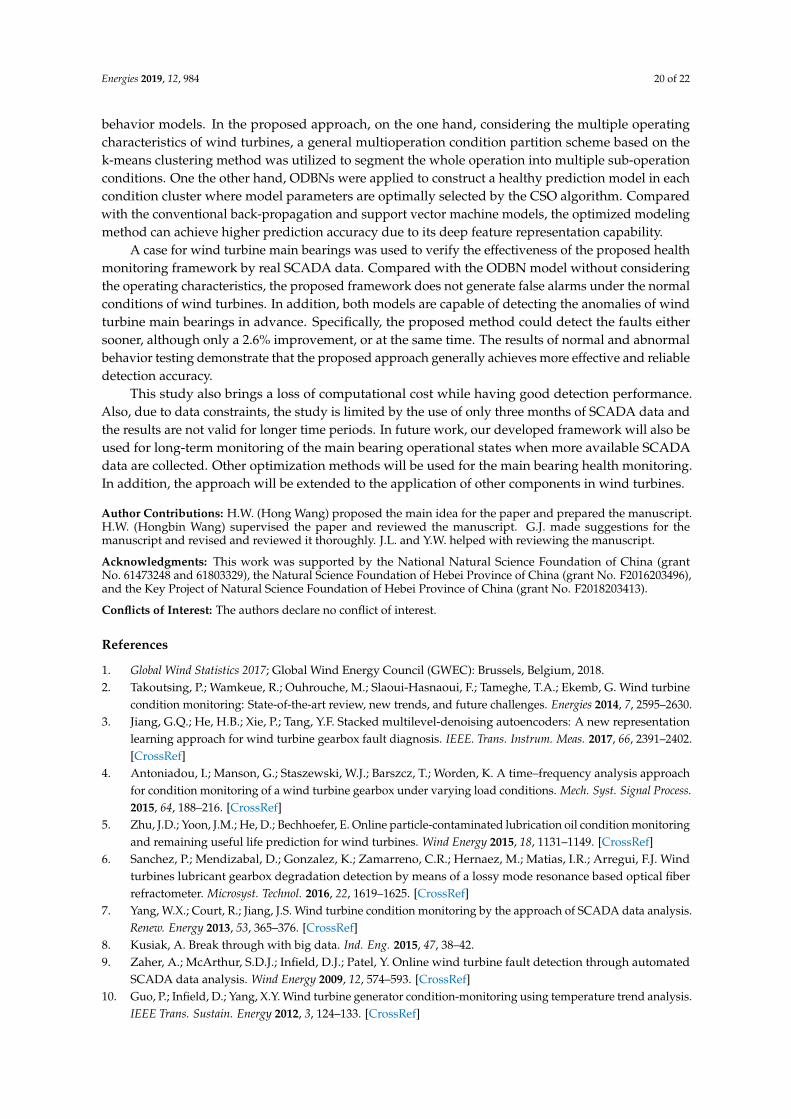
Energies 2019, 12, 984 20 of 22

behavior models. In the proposed approach, on the one hand, considering the multiple operatingcharacteristics of wind turbines, a general multioperation condition partition scheme based on thek-means clustering method was utilized to segment the whole operation into multiple sub-operationconditions. One the other hand, ODBNs were applied to construct a healthy prediction model in eachcondition cluster where model parameters are optimally selected by the CSO algorithm. Comparedwith the conventional back-propagation and support vector machine models, the optimized modelingmethod can achieve higher prediction accuracy due to its deep feature representation capability.

A case for wind turbine main bearings was used to verify the effectiveness of the proposed healthmonitoring framework by real SCADA data. Compared with the ODBN model without consideringthe operating characteristics, the proposed framework does not generate false alarms under the normalconditions of wind turbines. In addition, both models are capable of detecting the anomalies of windturbine main bearings in advance. Specifically, the proposed method could detect the faults eithersooner, although only a 2.6% improvement, or at the same time. The results of normal and abnormalbehavior testing demonstrate that the proposed approach generally achieves more effective and reliabledetection accuracy.

This study also brings a loss of computational cost while having good detection performance.Also, due to data constraints, the study is limited by the use of only three months of SCADA data andthe results are not valid for longer time periods. In future work, our developed framework will also beused for long-term monitoring of the main bearing operational states when more available SCADAdata are collected. Other optimization methods will be used for the main bearing health monitoring.In addition, the approach will be extended to the application of other components in wind turbines.

Author Contributions: H.W. (Hong Wang) proposed the main idea for the paper and prepared the manuscript.H.W. (Hongbin Wang) supervised the paper and reviewed the manuscript. G.J. made suggestions for themanuscript and revised and reviewed it thoroughly. J.L. and Y.W. helped with reviewing the manuscript.

Acknowledgments: This work was supported by the National Natural Science Foundation of China (grantNo. 61473248 and 61803329), the Natural Science Foundation of Hebei Province of China (grant No. F2016203496),and the Key Project of Natural Science Foundation of Hebei Province of China (grant No. F2018203413).

Conflicts of Interest: The authors declare no conflict of interest.

References

1. Global Wind Statistics 2017; Global Wind Energy Council (GWEC): Brussels, Belgium, 2018.2. Takoutsing, P.; Wamkeue, R.; Ouhrouche, M.; Slaoui-Hasnaoui, F.; Tameghe, T.A.; Ekemb, G. Wind turbine

condition monitoring: State-of-the-art review, new trends, and future challenges. Energies 2014, 7, 2595–2630.3. Jiang, G.Q.; He, H.B.; Xie, P.; Tang, Y.F. Stacked multilevel-denoising autoencoders: A new representation

learning approach for wind turbine gearbox fault diagnosis. IEEE. Trans. Instrum. Meas. 2017, 66, 2391–2402.[CrossRef]

4. Antoniadou, I.; Manson, G.; Staszewski, W.J.; Barszcz, T.; Worden, K. A time–frequency analysis approachfor condition monitoring of a wind turbine gearbox under varying load conditions. Mech. Syst. Signal Process.2015, 64, 188–216. [CrossRef]

5. Zhu, J.D.; Yoon, J.M.; He, D.; Bechhoefer, E. Online particle-contaminated lubrication oil condition monitoringand remaining useful life prediction for wind turbines. Wind Energy 2015, 18, 1131–1149. [CrossRef]

6. Sanchez, P.; Mendizabal, D.; Gonzalez, K.; Zamarreno, C.R.; Hernaez, M.; Matias, I.R.; Arregui, F.J. Windturbines lubricant gearbox degradation detection by means of a lossy mode resonance based optical fiberrefractometer. Microsyst. Technol. 2016, 22, 1619–1625. [CrossRef]

7. Yang, W.X.; Court, R.; Jiang, J.S. Wind turbine condition monitoring by the approach of SCADA data analysis.Renew. Energy 2013, 53, 365–376. [CrossRef]

8. Kusiak, A. Break through with big data. Ind. Eng. 2015, 47, 38–42.9. Zaher, A.; McArthur, S.D.J.; Infield, D.J.; Patel, Y. Online wind turbine fault detection through automated

SCADA data analysis. Wind Energy 2009, 12, 574–593. [CrossRef]10. Guo, P.; Infield, D.; Yang, X.Y. Wind turbine generator condition-monitoring using temperature trend analysis.

IEEE Trans. Sustain. Energy 2012, 3, 124–133. [CrossRef]

Energies 2019, 12, 984 21 of 22

11. Kusiak, A.; Verma, A. Analyzing bearing faults in wind turbines: A data-mining approach. Renew. Energy2012, 48, 110–116. [CrossRef]

12. Schlechtingen, M.; Santos, I.F.; Achiche, S. Wind turbine condition monitoring based on SCADA data usingnormal behavior models. Part 1: System description. Appl. Soft Comput. 2013, 13, 259–270. [CrossRef]

13. Schlechtingen, M.; Santos, I.F. Wind turbine condition monitoring based on SCADA data using normalbehavior models. Part 2: Application examples. Appl. Soft Comput. 2014, 14, 447–460. [CrossRef]

14. Bangalore, P.; Tjernberg, L.B. An artificial neural network approach for early fault detection of gearboxbearings. IEEE Trans. Smart Grid 2015, 6, 980–987. [CrossRef]

15. Bangalore, P.; Letzgus, S.; Karlsson, D.; Patriksson, M. An artificial neural network-based conditionmonitoring method for wind turbines, with application to the monitoring of the gearbox. Wind Energy 2017,20, 1421–1438. [CrossRef]

16. Bi, R.; Zhou, C.K.; Hepburn, D.M. Detection and classification of faults in pitch-regulated wind turbinegenerators using normal behaviour models based on performance curves. Renew. Energy 2017, 105, 674–688.[CrossRef]

17. Zhan, S.; Tao, Q.Q.; Li, X.H. Face detection using representation learning. Neurocomputing 2016, 187, 19–26.[CrossRef]

18. Wang, Y.; Wang, X.G.; Liu, W.Y. Unsupervised local deep feature for image recognition. Inf. Sci. 2016, 351,67–75. [CrossRef]

19. Jiang, G.Q.; Xie, P.; He, H.B.; Yan, J. Wind turbine fault detection using a denoising autoencoder withtemporal information. IEEE ASME Trans. Mechatron. 2018, 23, 89–100. [CrossRef]

20. Yang, Z.X.; Wang, X.B.; Zhong, J.H. Representational learning for fault diagnosis of wind turbine equipment:A multi-layered extreme learning machines approach. Energies 2016, 9, 379. [CrossRef]

21. Hinton, G.E.; Osindero, S.; Teh, Y.W. A fast learning algorithm for deep belief nets. Neural Comput. 2006, 18,1527–1554. [CrossRef]

22. Chen, H.Z.; Wang, J.X.; Tang, B.P.; Xiao, K.; Li, J.Y. An integrated approach to planetary gearbox faultdiagnosis using deep belief networks. Meas. Sci. Technol. 2017, 28, 025010. [CrossRef]

23. Wan, J.; Liu, J.F.; Ren, G.R.; Guo, Y.F.; Yu, D.R.; Hu, Q.H. Day-ahead prediction of wind speed with deepfeature learning. Int. J. Pattern Recognit. Artif. Intell. 2016, 30, 1650011. [CrossRef]

24. Chen, Z.Y.; Li, W.H. Multisensor feature fusion for bearing fault diagnosis using sparse autoencoder anddeep belief network. IEEE Trans. Instrum. Meas. 2017, 66, 1693–1702. [CrossRef]

25. Ren, H.; Chai, Y.; Qu, J.F.; Ye, X.; Tang, Q. A novel adaptive fault detection methodology for complex systemusing deep belief networks and multiple models: A case study on cryogenic propellant loading system.Neurocomputing 2018, 275, 2111–2125. [CrossRef]

26. Shao, H.D.; Jiang, H.K.; Zhang, X.; Niu, M.G. Rolling bearing fault diagnosis using an optimization deepbelief network. Meas. Sci. Technol. 2015, 26, 115002. [CrossRef]

27. Unal, M.; Onat, M.; Demetgul, M.; Kucuk, H. Fault diagnosis of rolling bearings using a genetic algorithmoptimized neural network. Measurement 2014, 58, 187–196. [CrossRef]

28. Qiao, W.; Lu, D.G. A survey on wind turbine condition monitoring and fault diagnosis-Part I: Componentsand subsystems. IEEE Trans. Ind. Electron. 2015, 62, 6536–6545. [CrossRef]

29. Kusiak, A.; Li, W.Y. The prediction and diagnosis of wind turbine faults. Renew. Energy 2011, 36, 16–23.[CrossRef]

30. Lapira, E.; Brisset, D.; Davari Ardakani, H.; Siegel, D.; Lee, J. Wind turbine performance assessment usingmulti-regime modeling approach. Renew. Energy 2012, 45, 86–95. [CrossRef]

31. Yang, H.H.; Huang, M.L.; Lai, C.M.; Jin, J.R. An approach combining data mining and control charts-basedmodel for fault detection in wind turbines. Renew. Energy 2018, 115, 808–816. [CrossRef]

32. Macqueen, J. Some methods for classification and analysis of multivariate observations. In Proceedings ofthe 5th Berkeley Symposium on Mathematical Statistics and Probability, Berkeley, CA, USA, 21 June–18 July1965; pp. 281–297.

33. Jain, A.K. Data clustering: 50 years beyond k-means. Pattern Recognit. Lett. 2010, 31, 651–666. [CrossRef]34. Rousseeuw, P. Silhouettes: A graphical aid to the interpretation and validation of cluster analysis. J. Comput.

Appl. Math. 1986, 20, 53–65. [CrossRef]

Energies 2019, 12, 984 22 of 22

35. Mazidi, P.; Bertling Tjernberg, L.; Sanz Bobi, M.A. Wind turbine prognostics and maintenance managementbased on a hybrid approach of neural networks and a proportional hazards model. Proc. Inst. Mech. Eng.Part O J. Risk Reliab. 2017, 231, 121–129. [CrossRef]

36. Fisher, R.A. Statistical methods for research workers. Int. J. Plant Sci. 1954, 21, 340–341.37. Best, D.J.; Roberts, D.E. Algorithm AS 89: The upper tail probabilities of Spearman’s rho. J. R. Stat. Soc. 1975,

24, 377–379. [CrossRef]38. Taylor, J.M.G. Kendall and Spearman correlation-coefficients in the presence of a blocking variable. Biometrics

1987, 43, 409–416. [CrossRef] [PubMed]39. Hinton, G.E. Training products of experts by minimizing contrastive divergence. Neural Comput. 2002, 14,

1771–1800. [CrossRef] [PubMed]40. Hinton, G.E. A practical guide to training restricted boltzmann machines. In Neural Networks: Tricks of the

Trade; Springer: Berlin, Germany, 2012; Volume 7700, pp. 599–619.41. Meng, X.B.; Liu, Y.; Gao, X.Z.; Zhang, H.Z. A new bio-inspired algorithm: Chicken swarm optimization.

In Swarm Intelligence; Springer International Publishing: Berlin, Germany, 2014; Volume 8794, pp. 86–94.42. Niu, G.; Singh, S.; Holland, S.W.; Pecht, M. Health monitoring of electronic products based on Mahalanobis

distance and Weibull decision metrics. Microelectron. Reliab. 2011, 51, 279–284. [CrossRef]43. Bai, Y.; Sun, Z.Z.; Zeng, B.; Deng, J.; Li, C. A multi-pattern deep fusion model for short-term bus passenger

flow forecasting. Appl. Soft Comput. 2017, 58, 669–680. [CrossRef]

© 2019 by the authors. Licensee MDPI, Basel, Switzerland. This article is an open accessarticle distributed under the terms and conditions of the Creative Commons Attribution(CC BY) license (http://creativecommons.org/licenses/by/4.0/).