Embed Size (px)
Citation preview
East African Community 26 March 2018
EAC Compendium of
Environment Statistics
1
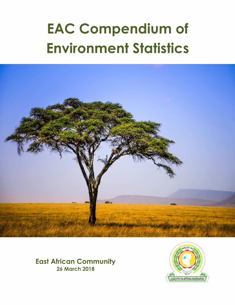
EAST AFRICAN COMMUNITY PARTNER STATES
South Sudan joined the East African Community in April 2016. Since they did not participate in the earlier part of the
project, their data could not be included in this Compendium.
2
TABLE OF CONTENTS
EAST AFRICAN COMMUNITY PARTNER STATES ...........................................................................................................1
LIST OF TABLES ..........................................................................................................................................................3
ACRONYMS AND ABBREVIATIONS ..............................................................................................................................6
UNITS OF MEASUREMENT ..........................................................................................................................................8
INTRODUCTION .........................................................................................................................................................9
FRAMEWORK ........................................................................................................................................................... 12
CHAPTER 1 ENVIRONMENTAL CONDITIONS AND QUALITY ........................................................................................ 15
Physical Conditions ............................................................................................................................................ 15
Land Cover, Ecosystems and Biodiversity ........................................................................................................ 20
Environmental Quality ....................................................................................................................................... 31
CHAPTER 2 ENVIRONMENTAL RESOURCES AND THEIR USE ....................................................................................... 33
Mineral Resources ............................................................................................................................................. 33
Energy Resources .............................................................................................................................................. 36
Land................................................................................................................................................................... 50
Biological Resources ......................................................................................................................................... 54
Water Resources ............................................................................................................................................... 59
CHAPTER 3 RESIDUALS ............................................................................................................................................. 65
Emissions to Air ................................................................................................................................................ 65
Generation and Management of Waste ................................................................................................................
Release of Chemical Substances ....................................................................................................................... 78
CHAPTER 4 EXTREME EVENTS AND DISASTERS .......................................................................................................... 85
Natural Extreme Events and Disasters ............................................................................................................. 85
Technological Disasters .................................................................................................................................... 94
CHAPTER 5 HUMAN SETTLEMENTS AND ENVIRONMENTAL HEALTH ........................................................................ 103
Human Settlements .........................................................................................................................................103
Environmental Health ..................................................................................................................................... 115
CHAPTER 6 ENVIRONMENTAL PROTECTION, MANAGEMENT AND ENGAGEMENT .................................................... 123
Environmental Governance and Protection .................................................................................................... 123
3
LIST OF TABLES
Table 1.1 Average monthly rainfall of capitals (mm/month) ...................................................................................... 16
Table 1.2 Long-term average precipitation in depth (mm/yr) and in volume (km3/yr) ................................................ 17
Table 1.3 Average maximum and minimum temperature (oC) (EAC facts and figures 2016 table 1.1f) ......................... 18
Table 1.4 Total surface area (103 km2) (EAC facts and figures 2016 table 1.1b) ........................................................... 19
Table 1.5 Total forest area (km2) ............................................................................................................................... 20
Table 1.6 Annual change rate of forest cover (% and 103 ha/yr) ................................................................................. 21
Table 1.7 Forest area within protected areas (km2) ................................................................................................... 22
Table 1.8 Proportion of forest protected area to the total forest area (%) .................................................................. 23
Table 1.9 Forest area as a proportion of total land area (%) [SDG 15.1.1] ................................................................... 24
Table 1.10 Proportion of important sites for terrestrial and freshwater biodiversity that are covered by protected
areas, by ecosystem type (%) [SDG 15.1.2] ................................................................................................................ 25
Table 1.11 Coverage by protected areas of important sites for mountain biodiversity (%) [SDG 15.4.1] ...................... 26
Table 1.12 Red List Index (mean, lower and upper bound) [SDG 15.5.1] ..................................................................... 27
Table 1.13 Number of threatened species by taxonomic group (number) [SDG 15.5.1] ............................................... 28
Table 1.14 Number of animals in each Red List Category (number) ............................................................................ 28
Table 1.15 Number of plants in each Red List Category (number) .............................................................................. 28
Table 1.16 Official development assistance and public expenditure on conservation and sustainable use of biodiversity
and ecosystems (million USD) [SDG 15.a.1 and SDG 15.b.1] ....................................................................................... 30
Table 1.17 Annual mean level of fine particulate matter (e.g. PM2.5 and PM10) in cities (population weighted) (%) [SDG
11.6.2] ..................................................................................................................................................................... 31
Table 2.1 Mineral production (EAC facts and figures 2016 table 4.3) .......................................................................... 34
Table 2.2 Electricity generation (GWh) (EAC facts and figures 2016 table 4.2b) .......................................................... 36
Table 2.3 Energy exports and imports (EAC facts and figures 2016 table 4.2c) ............................................................ 37
Table 2.4 Proportion of population with primary reliance on clean fuels and technology (%) [SDG 7.1.2] ................... 38
Table 2.5 Renewable energy share in the total final energy consumption (%) [SDG 7.2.1] .......................................... 39
Table 2.6 Energy intensity measured in terms of primary energy and GDP (MJ per USD constant 2011 PPP GDP) [SDG
7.3.1] ....................................................................................................................................................................... 40
Table 2.7 Total final consumption and its components (PJ and GJ per capita) ............................................................. 41
Table 2.8 Energy production ..................................................................................................................................... 43
Table 2.9 Material footprint (metric tons), material footprint per capita (metric tons) and material footprint per GDP
(kg) [SDG 8.4.1 and SDG 12.2.1] ................................................................................................................................ 46
Table 2.10 Domestic material consumption (metric tons), domestic material consumption per capita (kg), and
domestic material consumption per unit of GDP (metric tons) [SDG 8.4.2] ................................................................ 48
Table 2.11 Agricultural land use (103 ha) (EAC facts and figures 2016 table 1.1c) ........................................................ 50
4
Table 2.12 Total area equipped for irrigation (103 ha) ................................................................................................ 50
Table 2.13 Progress towards sustainable forest management [SDG 15.2.1] ................................................................ 52
Table 2.14 Livestock population by type (103 head) (EAC facts and figures 2016 table 4.1d)........................................ 54
Table 2.15 Fish catch (103 t) (EAC facts and figures 2016 table 4.1e) ........................................................................... 55
Table 2.16 Fisheries production by aquaculture (Quantity (tonnes) and Value (1,000 USD)) ....................................... 55
Table 2.17 Coverage of protected areas in relation to marine areas (%) [SDG 14.5.1] ................................................. 56
Table 2.18 Production for selected crops, (103 t) (EAC facts and figures 2016 table 4.1b) ............................................ 57
Table 2.19 Production of exports and imports of forest products (1,000 USD) ............................................................ 57
Table 2.20 Total internal renewable water resources (km3/yr) .................................................................................. 59
Table 2.21 Total external renewable water resources (km3/yr) .................................................................................. 60
Table 2.22 Level of water stress: freshwater withdrawal as a proportion of available freshwater resources (%) [SDG
6.4.2] ....................................................................................................................................................................... 61
Table 2.23 Water supply industry (million m3/y) ....................................................................................................... 62
Table 2.24 Degree of integrated water resources management implementation (0-100) (SDG 6.5.1) .......................... 63
Table 3.1 Fossil fuel CO2 emissions (103 mt C)* .......................................................................................................... 65
Table 3.2 CO2 emissions per unit of value added [SDG 9.4.1] ..................................................................................... 67
Table 3.3 Emissions of direct greenhouse gases (CO2, CH4, N2O) ................................................................................. 69
Table 3.4 Ozone-depleting substances (ODS) consumption (ODP tonnes) .................................................................. 71
Table 3.5 Total waste generation (1,000 tonnes) ....................................................................................................... 73
Table 3.6 Municipal waste collected – national level (1,000 tonnes) .......................................................................... 74
Table 3.7 Municipal waste collected – capital city (1,000 tonnes) .............................................................................. 75
Table 3.8 Municipal waste treated or disposed – capital city (1,000 tonnes) .............................................................. 75
Table 3.9 Composition of municipal waste (%) .......................................................................................................... 77
Table 3.10 Consumption of fertilizers (tonnes of nutrients) ....................................................................................... 78
Table 3.11 Consumption of fertilizers per 1,000 hectares of agricultural land area (tonnes of nutrients) ..................... 80
Table 3.12 Use of pesticides (tonnes of active ingredients) ........................................................................................ 81
Table 4.1 Natural disasters ....................................................................................................................................... 85
Table 4.2 Number of deaths, missing persons and persons affected by disaster per 100,000 people (number) [SDG
1.5.1 and SDG 11.5.1 and SDG 13.1.1] ....................................................................................................................... 91
Table 4.3 Direct disaster economic loss in relation to global GDP, including disaster damage to critical infrastructure
and disruption of basic services (per 1,000 USD) [SDG 11.5.2] ................................................................................... 93
Table 4.4 Industrial accidents ................................................................................................................................... 94
Table 4.5 Transport accidents ................................................................................................................................... 96
Table 4.6 Miscellaneous accidents .......................................................................................................................... 100
Table 5.1 Proportion of population using safely managed drinking water services (%) [SDG 6.1.1] ........................... 104
Table 5.2 Proportion of population practicing open defecation (%) [SDG 6.2.1] ........................................................ 105
5
Table 5.3 Proportion of population with basic handwashing facilities on premises (%) [SDG 6.2.1] ........................... 105
Table 5.4 Proportion of urban population living in slums, informal settlements or inadequate housing (%, number 103)
[SDG 11.1.1]........................................................................................................................................................... 106
Table 5.5 Total population living within the low elevation coastal zone (LECZ) (number) .......................................... 108
Table 5.6 Proportion of population living in low elevation coastal zone (LECZ) (%) ................................................... 109
Table 5.7 Proportion of population with access to electricity (%) [SDG 7.1.1] ........................................................... 110
Table 5.8 Electricity access in 2016 (%) .................................................................................................................... 111
Table 5.9 Total population supplied by water supply industry (%) ........................................................................... 112
Table 5.10 Population connected to wastewater collecting system (%) .................................................................... 113
Table 5.11 Amount of water-and sanitation-related official development assistance that is part of a government-
coordinated spending plan (billions) [SDG 6.a.1] ..................................................................................................... 114
Table 5.12 Cholera fatality rates, reported cases and deaths (number) .................................................................... 115
Table 5.13 Malaria fatality rates, reported cases and deaths (number) .................................................................... 116
Table 5.14 Yellow fever reported (number)............................................................................................................. 117
Table 5.15 Mortality rate attributed to household and ambient air pollution (per 100,000 population) [SDG 3.9.1] .. 118
Table 5.16 Mortality rate attributed to unsafe water, unsafe sanitation and lack of hygiene (exposure to unsafe
Water, Sanitation and Hygiene for All (WASH) services) (per 100,000 population) [SDG 3.9.2] ................................. 119
Table 5.17 Countries with a high level of users/communities participating in planning programs in drinking-water
supply [SDG 6.b.1] ................................................................................................................................................. 120
Table 5.18 Countries with a high level of users/communities participating in planning programs in hygiene promotion
[SDG 6.b.1] ............................................................................................................................................................ 120
Table 5.19 Countries with a high level of users/communities participating in planning programs in sanitation [SDG
6.b.1] ..................................................................................................................................................................... 121
Table 6.1 Participation in multilateral environmental agreements (MEAs) and other global environmental
conventions: List and description ........................................................................................................................... 123
Table 6.2 Number of parties to international multilateral environmental agreements on hazardous waste, and other
chemicals that meet their commitments and obligations in transmitting information as required by each relevant
agreement (number) [SDG 12.4.1] .......................................................................................................................... 124
6
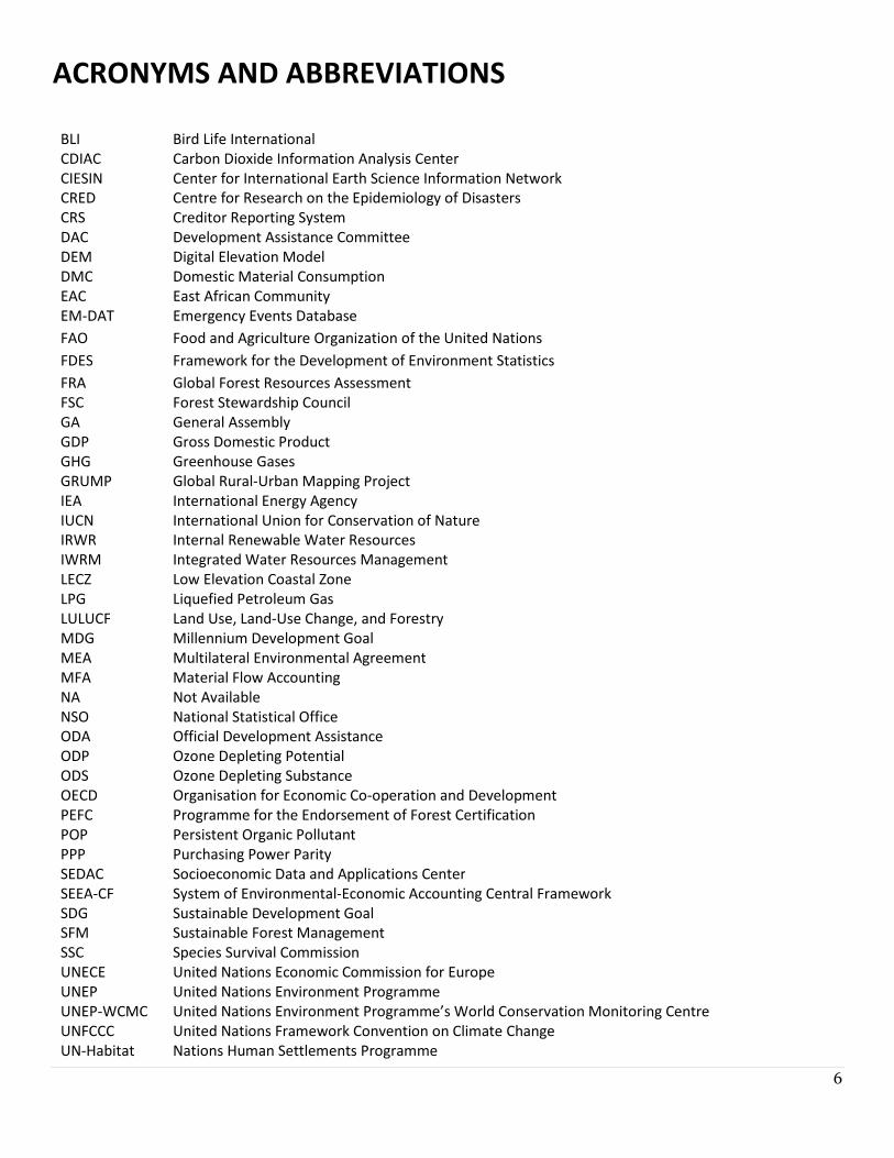
ACRONYMS AND ABBREVIATIONS
BLI Bird Life International
CDIAC Carbon Dioxide Information Analysis Center
CIESIN Center for International Earth Science Information Network
CRED Centre for Research on the Epidemiology of Disasters
CRS Creditor Reporting System
DAC Development Assistance Committee
DEM Digital Elevation Model
DMC Domestic Material Consumption
EAC East African Community
EM-DAT Emergency Events Database
FAO Food and Agriculture Organization of the United Nations
FDES Framework for the Development of Environment Statistics
FRA
FSC
GA
Global Forest Resources Assessment
Forest Stewardship Council
General Assembly
GDP Gross Domestic Product
GHG Greenhouse Gases
GRUMP Global Rural-Urban Mapping Project
IEA International Energy Agency
IUCN International Union for Conservation of Nature
IRWR Internal Renewable Water Resources
IWRM Integrated Water Resources Management
LECZ Low Elevation Coastal Zone
LPG Liquefied Petroleum Gas
LULUCF Land Use, Land-Use Change, and Forestry
MDG Millennium Development Goal
MEA Multilateral Environmental Agreement
MFA Material Flow Accounting
NA Not Available
NSO National Statistical Office
ODA Official Development Assistance
ODP Ozone Depleting Potential
ODS Ozone Depleting Substance
OECD Organisation for Economic Co-operation and Development
PEFC Programme for the Endorsement of Forest Certification
POP Persistent Organic Pollutant
PPP Purchasing Power Parity
SEDAC Socioeconomic Data and Applications Center
SEEA-CF System of Environmental-Economic Accounting Central Framework
SDG
SFM
Sustainable Development Goal
Sustainable Forest Management
SSC Species Survival Commission
UNECE United Nations Economic Commission for Europe
UNEP United Nations Environment Programme
UNEP-WCMC United Nations Environment Programme’s World Conservation Monitoring Centre
UNFCCC United Nations Framework Convention on Climate Change
UN-Habitat Nations Human Settlements Programme

7
UNICEF United Nations Children’s Fund
UNIDO United Nations Industrial Development Organization
UNISDR United Nations International Strategy for Disaster Reduction
UNSD United Nations Statistics Division
WASH Water, Sanitation and Hygiene for All
WDPA World Database on Protected Areas
WHO
WMO
World Health Organization
World Meteorological Organization
8
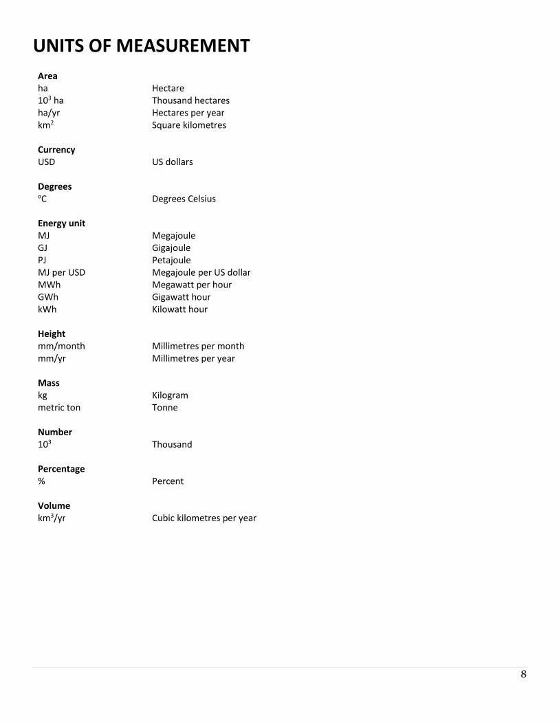
UNITS OF MEASUREMENT
Area
ha Hectare
103 ha Thousand hectares
ha/yr Hectares per year
km2 Square kilometres
Currency
USD US dollars
Degrees oC Degrees Celsius
Energy unit
MJ Megajoule
GJ Gigajoule
PJ Petajoule
MJ per USD Megajoule per US dollar
MWh Megawatt per hour
GWh Gigawatt hour
kWh Kilowatt hour
Height
mm/month Millimetres per month
mm/yr Millimetres per year
Mass
kg Kilogram
metric ton Tonne
Number
103 Thousand
Percentage
% Percent
Volume
km3/yr Cubic kilometres per year

9
10
INTRODUCTION
Environment statistics provide information about the state and changes of environmental conditions, the quality and
availability of environmental resources, the impact of human activities and natural events on the environment and the
impact of changing environmental conditions. They also provide information about the social actions and economic
measures that societies take to avoid or mitigate these impacts and to restore and maintain the capacity of the
environment to provide the services that are essential for life and human well-being1.
The EAC Compendium of Environment Statistics was prepared by the United Nations Statistics Division (UNSD), in
collaboration with the East African Community (EAC), as part of the United Nations Development Account Project entitled
“Supporting Member States in developing and strengthening environment statistics and integrated environmental-
economic accounting for improved monitoring of sustainable development”. The principal objective of the Compendium
is to provide a first regional compilation of comparable data on short and long-term trends of environment statistics.
This project, which took place from 2015 to 2017, included two modules. Module A focused on strengthening environment
statistics in the EAC Secretariat and its five member states, Burundi, Kenya, Rwanda, the United Republic of Tanzania and
Uganda2. For Module A, the strategy adopted for the implementation of the project included the following elements: (i)
an initial sub-regional workshop to build national capacities; (ii) national missions to each project country composed of
meetings with key stakeholders and a training workshop; (iii) engaging national consultants for each project country to
support the development of a national plan for environment statistics and a national compendium of environment
statistics; and (iv) two further sub-regional workshops to review the progress in the implementation of the FDES and the
Environment Statistics Self-Assessment Tool (ESSAT), and develop two additional outputs not originally included in the
project, this regional EAC Compendium of Environment Statistics and a Regional Action Plan for Environment Statistics.
On 25 September 2015, countries adopted a set of goals to end poverty, protect the planet and ensure prosperity for all
as part of a new sustainable development agenda. Each goal has specific targets to be achieved over the next 15 years3.
To monitor these targets, a global indicator framework was developed by the Inter-Agency and Expert Group on SDG
Indicators (IAEG-SDGs) and adopted by the United Nations Statistical Commission in March 2017 and by the United Nations
General Assembly in July 2017. This set of indicators is intended for the review of progress at the global level4. The
Compendium reflects this global indicator framework by including the environmentally-related SDG indicators for which
there are data available. Data in the Compendium have also been sourced from the EAC Facts and Figures 20165 as well
as from international and regional organizations.
Each chapter of the Compendium refers to one of the six components of the Framework for the Development of
Environment Statistics (FDES 2013)6. Data availability per country varies among the different tables. For the complete time
series for each table the original source should be consulted.
Metadata for the tables have been provided where available. Footnotes for the SDG indicator tables are described on the
next page. Footnotes for other sources are indicated below each table. Description of notes and symbols are displayed
below each table.
1 https://unstats.un.org/unsd/environment/FDES/FDES-2015-supporting-tools/FDES.pdf 2 https://unstats.un.org/unsd/envstats/EAC/ 3 http://www.un.org/sustainabledevelopment/sustainable-development-goals/ 4 https://unstats.un.org/sdgs/files/report/2017/TheSustainableDevelopmentGoalsReport2017.pdf 5 https://www.eac.int/documents/category/key-documents 6 https://unstats.un.org/unsd/environment/FDES/FDES-2015-supporting-tools/FDES.pdf
11
Footnotes for SDG Indicator Tables
Footnotes in letters for data from the SDGs database indicate the datatypes, e.g. 45.87E, E stands for estimated. All data
type footnotes in this book are listed as following:
Country Data (C): the figure is the one produced and disseminated by the country (including data adjusted BY THE
COUNTRY to meet international standards).
Estimated (E): The figure is estimated by the international agency, when corresponding country data on a specific year or
set of years are not available, or when multiple sources exist, or there are issues of data quality. Estimates are based on
national data, such as surveys or administrative records, or other sources but on the same variable being estimated.
Global monitoring data (G): The figure is regularly produced by the designated agency for the global monitoring, based on
country data. However, there is no corresponding figure at the country level, because the indicator is defined for
international monitoring only (example: population below 1$ a day).
Modeled (M): The figure is modeled by the agency when there is a complete lack of data on the variable being estimated.
The model is based on a set of covariates—other variables for which data are available and that can explain the
phenomenon.
Data type not available (NA): A figure was not provided, or the "nature of data" is unknown.
12
FRAMEWORK
This Compendium is based on the structure of the Framework for the Development of Environment Statistics (FDES 2013)7
developed by the United Nations Statistics Division (UNSD). The FDES 2013 is a flexible, multi-purpose conceptual and
statistical framework that is comprehensive and integrative in nature. It marks out the scope of environment statistics and
provides an organizing structure to guide their collection and compilation and to synthesize data from various subject
areas and sources, covering the issues and aspects of the environment that are relevant for analysis, policy and decision
making.
The scope of the FDES covers biophysical aspects of the environment, those aspects of the human sub-system that directly
influence the state and quality of the environment, and the impacts of the changing environment on the human sub-
system. It includes interactions within and among the environment, human activities and natural events.
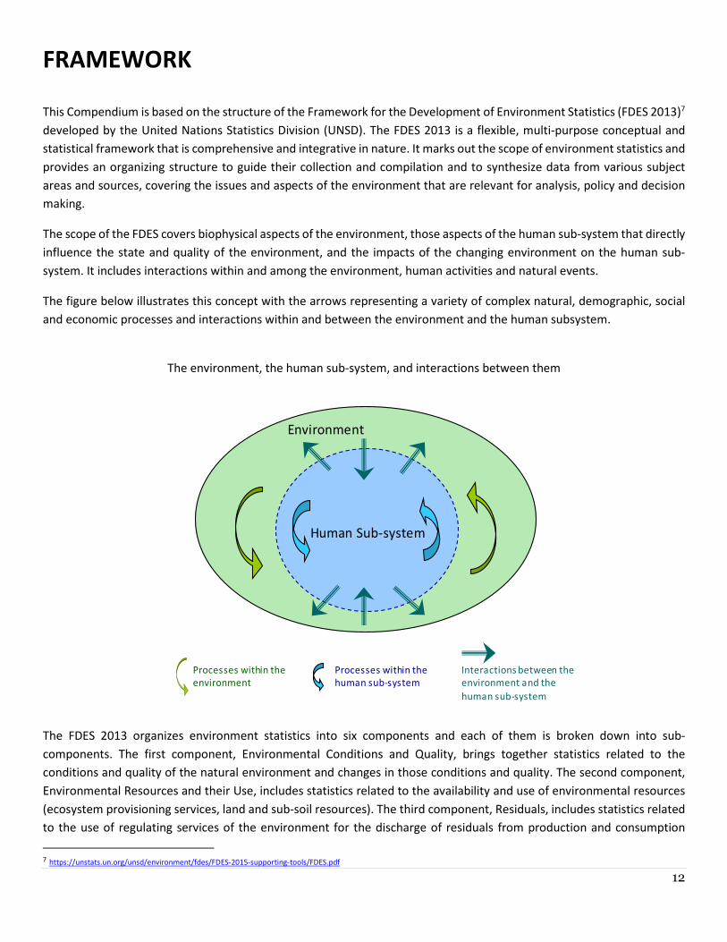
The figure below illustrates this concept with the arrows representing a variety of complex natural, demographic, social
and economic processes and interactions within and between the environment and the human subsystem.
The environment, the human sub-system, and interactions between them
Human Sub-system
Interactions between the
environment and the
human sub-system
Processes within the
environment
Processes within the
human sub-system
Environment
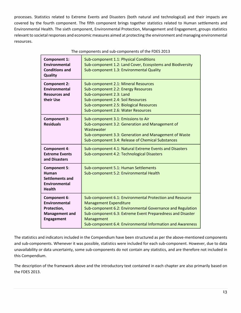
The FDES 2013 organizes environment statistics into six components and each of them is broken down into sub-
components. The first component, Environmental Conditions and Quality, brings together statistics related to the
conditions and quality of the natural environment and changes in those conditions and quality. The second component,
Environmental Resources and their Use, includes statistics related to the availability and use of environmental resources
(ecosystem provisioning services, land and sub-soil resources). The third component, Residuals, includes statistics related
to the use of regulating services of the environment for the discharge of residuals from production and consumption
7 https://unstats.un.org/unsd/environment/fdes/FDES-2015-supporting-tools/FDES.pdf
13
processes. Statistics related to Extreme Events and Disasters (both natural and technological) and their impacts are
covered by the fourth component. The fifth component brings together statistics related to Human settlements and
Environmental Health. The sixth component, Environmental Protection, Management and Engagement, groups statistics
relevant to societal responses and economic measures aimed at protecting the environment and managing environmental
resources.
The components and sub-components of the FDES 2013
Component 1:
Environmental
Conditions and
Quality
Sub-component 1.1: Physical Conditions
Sub-component 1.2: Land Cover, Ecosystems and Biodiversity
Sub-component 1.3: Environmental Quality
Component 2:
Environmental
Resources and
their Use
Sub-component 2.1: Mineral Resources
Sub-component 2.2: Energy Resources
Sub-component 2.3: Land
Sub-component 2.4: Soil Resources
Sub-component 2.5: Biological Resources
Sub-component 2.6: Water Resources
Component 3:
Residuals
Sub-component 3.1: Emissions to Air
Sub-component 3.2: Generation and Management of
Wastewater
Sub-component 3.3: Generation and Management of Waste
Sub-component 3.4: Release of Chemical Substances
Component 4:
Extreme Events
and Disasters
Sub-component 4.1: Natural Extreme Events and Disasters
Sub-component 4.2: Technological Disasters
Component 5:
Human
Settlements and
Environmental
Health
Sub-component 5.1: Human Settlements
Sub-component 5.2: Environmental Health
Component 6:
Environmental
Protection,
Management and
Engagement
Sub-component 6.1: Environmental Protection and Resource
Management Expenditure
Sub-component 6.2: Environmental Governance and Regulation
Sub-component 6.3: Extreme Event Preparedness and Disaster
Management
Sub-component 6.4: Environmental Information and Awareness
The statistics and indicators included in the Compendium have been structured as per the above-mentioned components
and sub-components. Whenever it was possible, statistics were included for each sub-component. However, due to data
unavailability or data uncertainty, some sub-components do not contain any statistics, and are therefore not included in
this Compendium.
The description of the framework above and the introductory text contained in each chapter are also primarily based on
the FDES 2013.
14
Chapter 1
Environmental Conditions and Quality
15
CHAPTER 1 ENVIRONMENTAL CONDITIONS AND QUALITY
This chapter based on the FDES Component 1 on Environmental Conditions and Quality includes statistics about the
physical, biological and chemical characteristics of the environment and their changes over time. These conditions
determine the ecosystems characteristics and will vary in space and time as a result of natural processes and/or human
influence. These fundamental background conditions are strongly interrelated and determine the types, extent, conditions
and health of ecosystems. Many of these natural conditions change very slowly as a result of natural processes or human
influence. Others may show immediate and dramatic effects. Importantly, changes in environmental conditions and
quality are the result of combined and accumulated impacts of natural and human processes. Connecting the changes
with individual activities or events is thus not a straightforward process.
Physical Conditions Physical conditions is designed to capture physical aspects of the environment which change relatively slowly because of
human influence. Statistics on meteorological, hydrographical, and geographical characteristics are included below. These
conditions are important as they help determine the scope of and influences on the environmental resources of a country.
16
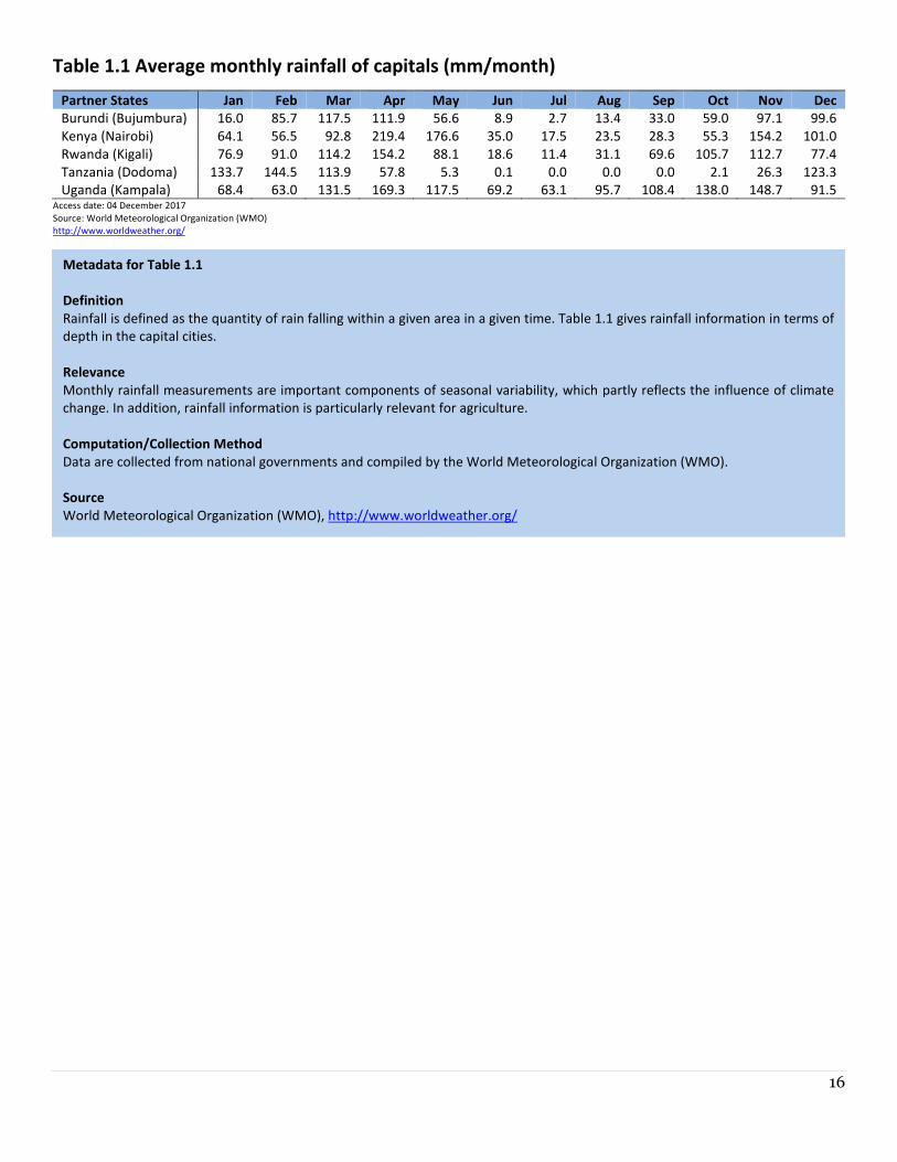
Table 1.1 Average monthly rainfall of capitals (mm/month)
Partner States Jan Feb Mar Apr May Jun Jul Aug Sep Oct Nov Dec
Burundi (Bujumbura) 16.0 85.7 117.5 111.9 56.6 8.9 2.7 13.4 33.0 59.0 97.1 99.6
Kenya (Nairobi) 64.1 56.5 92.8 219.4 176.6 35.0 17.5 23.5 28.3 55.3 154.2 101.0
Rwanda (Kigali) 76.9 91.0 114.2 154.2 88.1 18.6 11.4 31.1 69.6 105.7 112.7 77.4
Tanzania (Dodoma) 133.7 144.5 113.9 57.8 5.3 0.1 0.0 0.0 0.0 2.1 26.3 123.3
Uganda (Kampala) 68.4 63.0 131.5 169.3 117.5 69.2 63.1 95.7 108.4 138.0 148.7 91.5 Access date: 04 December 2017
Source: World Meteorological Organization (WMO)
http://www.worldweather.org/
Metadata for Table 1.1
Definition
Rainfall is defined as the quantity of rain falling within a given area in a given time. Table 1.1 gives rainfall information in terms of
depth in the capital cities.
Relevance
Monthly rainfall measurements are important components of seasonal variability, which partly reflects the influence of climate
change. In addition, rainfall information is particularly relevant for agriculture.
Computation/Collection Method
Data are collected from national governments and compiled by the World Meteorological Organization (WMO).
Source
World Meteorological Organization (WMO), http://www.worldweather.org/
17
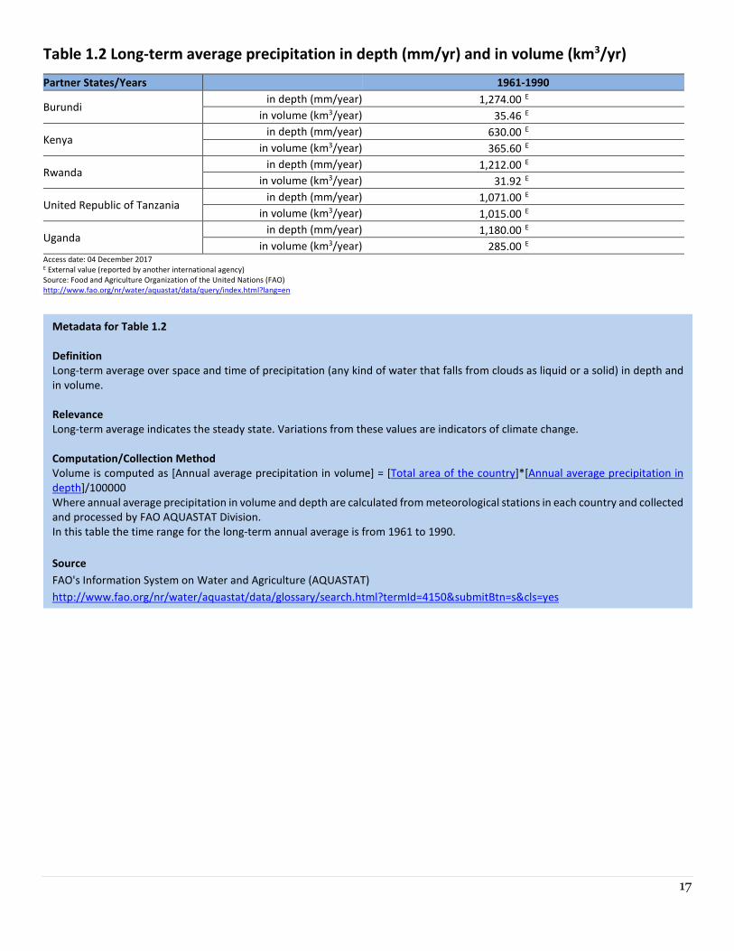
Table 1.2 Long-term average precipitation in depth (mm/yr) and in volume (km3/yr)
Partner States/Years 1961-1990
Burundi in depth (mm/year) 1,274.00 E
in volume (km3/year) 35.46 E
Kenya in depth (mm/year) 630.00 E
in volume (km3/year) 365.60 E
Rwanda in depth (mm/year) 1,212.00 E
in volume (km3/year) 31.92 E
United Republic of Tanzania in depth (mm/year) 1,071.00 E
in volume (km3/year) 1,015.00 E
Uganda in depth (mm/year) 1,180.00 E
in volume (km3/year) 285.00 E
Access date: 04 December 2017 E External value (reported by another international agency)
Source: Food and Agriculture Organization of the United Nations (FAO)
http://www.fao.org/nr/water/aquastat/data/query/index.html?lang=en
Metadata for Table 1.2
Definition
Long-term average over space and time of precipitation (any kind of water that falls from clouds as liquid or a solid) in depth and
in volume.
Relevance
Long-term average indicates the steady state. Variations from these values are indicators of climate change.
Computation/Collection Method
Volume is computed as [Annual average precipitation in volume] = [Total area of the country]*[Annual average precipitation in
depth]/100000
Where annual average precipitation in volume and depth are calculated from meteorological stations in each country and collected
and processed by FAO AQUASTAT Division.
In this table the time range for the long-term annual average is from 1961 to 1990.
Source
FAO's Information System on Water and Agriculture (AQUASTAT)
http://www.fao.org/nr/water/aquastat/data/glossary/search.html?termId=4150&submitBtn=s&cls=yes
18
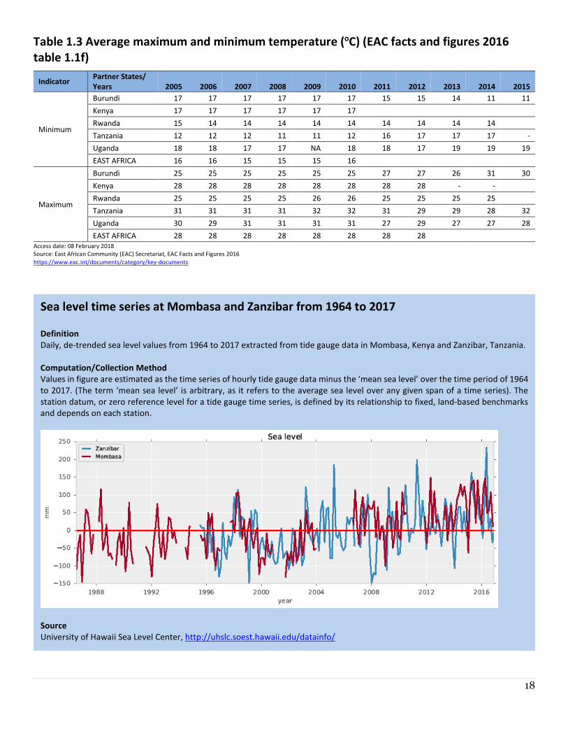
Table 1.3 Average maximum and minimum temperature (oC) (EAC facts and figures 2016
table 1.1f)
Indicator Partner States/
Years 2005 2006 2007 2008 2009 2010 2011 2012 2013 2014 2015
Minimum
Burundi 17 17 17 17 17 17 15 15 14 11 11
Kenya 17 17 17 17 17 17
Rwanda 15 14 14 14 14 14 14 14 14 14
Tanzania 12 12 12 11 11 12 16 17 17 17 -
Uganda 18 18 17 17 NA 18 18 17 19 19 19
EAST AFRICA 16 16 15 15 15 16
Maximum
Burundi 25 25 25 25 25 25 27 27 26 31 30
Kenya 28 28 28 28 28 28 28 28 - -
Rwanda 25 25 25 25 26 26 25 25 25 25
Tanzania 31 31 31 31 32 32 31 29 29 28 32
Uganda 30 29 31 31 31 31 27 29 27 27 28
EAST AFRICA 28 28 28 28 28 28 28 28
Access date: 08 February 2018
Source: East African Community (EAC) Secretariat, EAC Facts and Figures 2016
https://www.eac.int/documents/category/key-documents
Sea level time series at Mombasa and Zanzibar from 1964 to 2017
Definition
Daily, de-trended sea level values from 1964 to 2017 extracted from tide gauge data in Mombasa, Kenya and Zanzibar, Tanzania.
Computation/Collection Method
Values in figure are estimated as the time series of hourly tide gauge data minus the ‘mean sea level’ over the time period of 1964
to 2017. (The term ‘mean sea level’ is arbitrary, as it refers to the average sea level over any given span of a time series). The
station datum, or zero reference level for a tide gauge time series, is defined by its relationship to fixed, land-based benchmarks
and depends on each station.
Source
University of Hawaii Sea Level Center, http://uhslc.soest.hawaii.edu/datainfo/
19
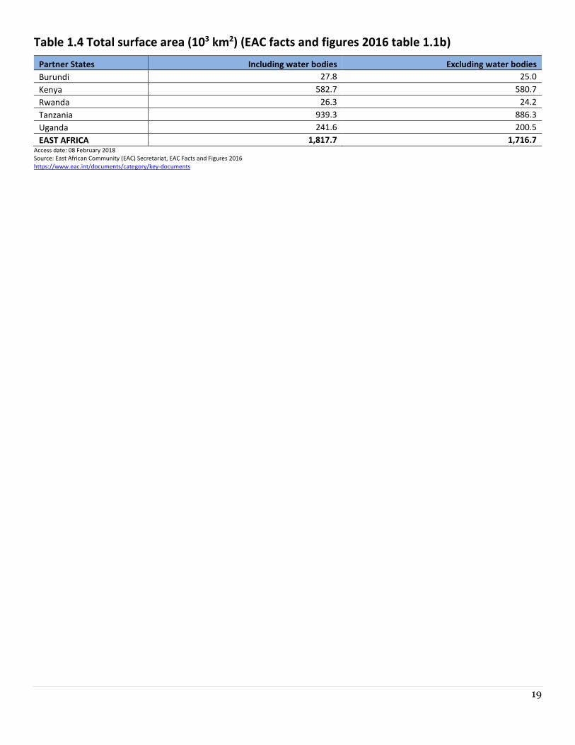
Table 1.4 Total surface area (103 km2) (EAC facts and figures 2016 table 1.1b)
Partner States Including water bodies Excluding water bodies
Burundi 27.8 25.0
Kenya 582.7 580.7
Rwanda 26.3 24.2
Tanzania 939.3 886.3
Uganda 241.6 200.5
EAST AFRICA 1,817.7 1,716.7 Access date: 08 February 2018
Source: East African Community (EAC) Secretariat, EAC Facts and Figures 2016
https://www.eac.int/documents/category/key-documents
20
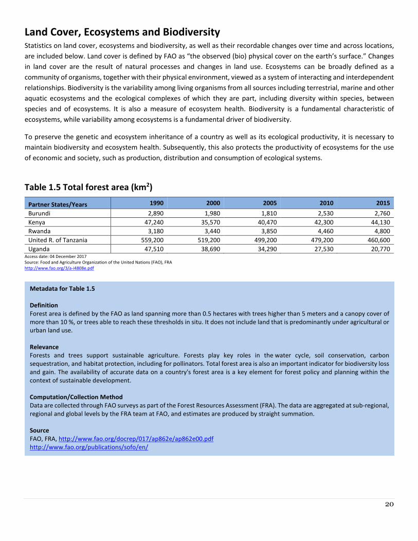
Land Cover, Ecosystems and Biodiversity Statistics on land cover, ecosystems and biodiversity, as well as their recordable changes over time and across locations,
are included below. Land cover is defined by FAO as “the observed (bio) physical cover on the earth’s surface.” Changes
in land cover are the result of natural processes and changes in land use. Ecosystems can be broadly defined as a
community of organisms, together with their physical environment, viewed as a system of interacting and interdependent
relationships. Biodiversity is the variability among living organisms from all sources including terrestrial, marine and other
aquatic ecosystems and the ecological complexes of which they are part, including diversity within species, between
species and of ecosystems. It is also a measure of ecosystem health. Biodiversity is a fundamental characteristic of
ecosystems, while variability among ecosystems is a fundamental driver of biodiversity.
To preserve the genetic and ecosystem inheritance of a country as well as its ecological productivity, it is necessary to
maintain biodiversity and ecosystem health. Subsequently, this also protects the productivity of ecosystems for the use
of economic and society, such as production, distribution and consumption of ecological systems.
Table 1.5 Total forest area (km2)
Partner States/Years 1990 2000 2005 2010 2015
Burundi 2,890 1,980 1,810 2,530 2,760
Kenya 47,240 35,570 40,470 42,300 44,130
Rwanda 3,180 3,440 3,850 4,460 4,800
United R. of Tanzania 559,200 519,200 499,200 479,200 460,600
Uganda 47,510 38,690 34,290 27,530 20,770 Access date: 04 December 2017
Source: Food and Agriculture Organization of the United Nations (FAO), FRA
http://www.fao.org/3/a-i4808e.pdf
Metadata for Table 1.5
Definition
Forest area is defined by the FAO as land spanning more than 0.5 hectares with trees higher than 5 meters and a canopy cover of
more than 10 %, or trees able to reach these thresholds in situ. It does not include land that is predominantly under agricultural or
urban land use.
Relevance
Forests and trees support sustainable agriculture. Forests play key roles in the water cycle, soil conservation, carbon
sequestration, and habitat protection, including for pollinators. Total forest area is also an important indicator for biodiversity loss
and gain. The availability of accurate data on a country's forest area is a key element for forest policy and planning within the
context of sustainable development.
Computation/Collection Method
Data are collected through FAO surveys as part of the Forest Resources Assessment (FRA). The data are aggregated at sub-regional,
regional and global levels by the FRA team at FAO, and estimates are produced by straight summation.
Source
FAO, FRA, http://www.fao.org/docrep/017/ap862e/ap862e00.pdf
http://www.fao.org/publications/sofo/en/
21
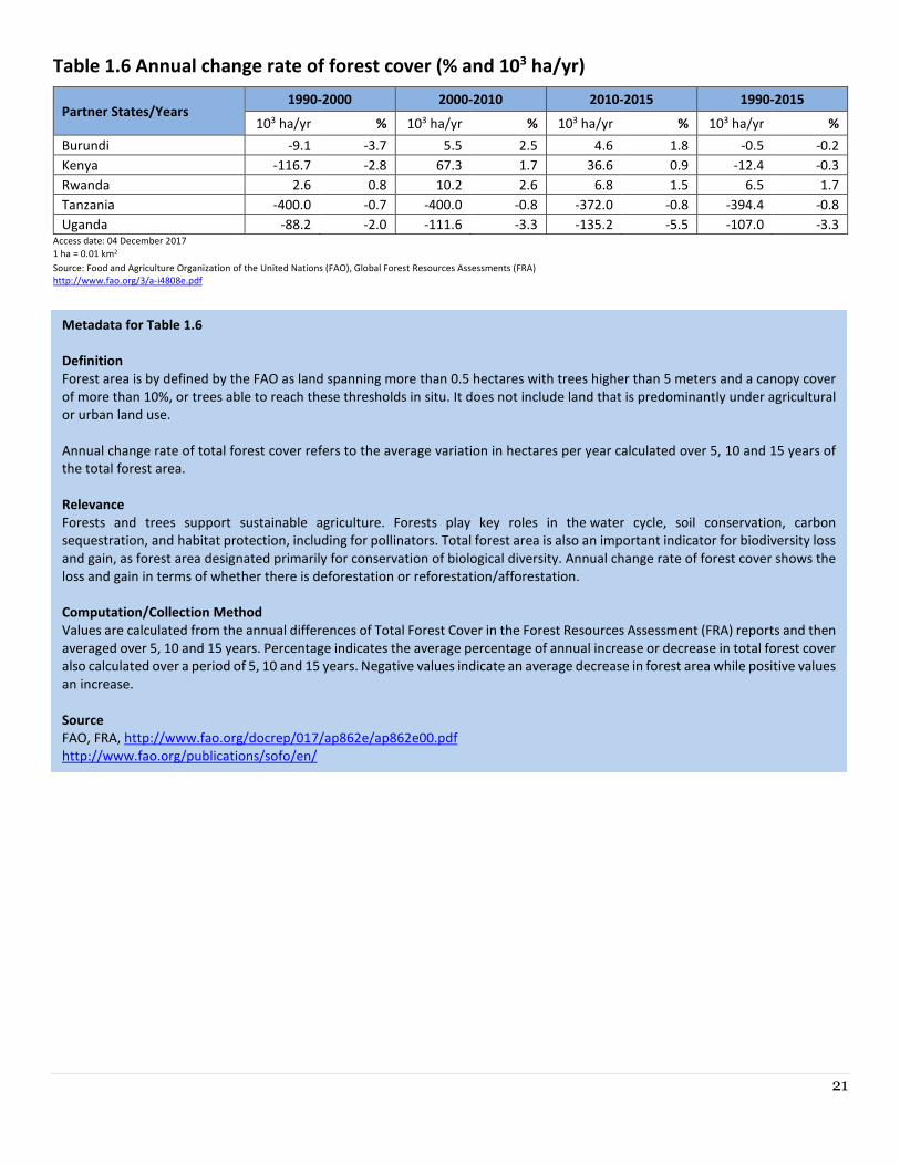
Table 1.6 Annual change rate of forest cover (% and 103 ha/yr)
Partner States/Years 1990-2000 2000-2010 2010-2015 1990-2015
103 ha/yr % 103 ha/yr % 103 ha/yr % 103 ha/yr %
Burundi -9.1 -3.7 5.5 2.5 4.6 1.8 -0.5 -0.2
Kenya -116.7 -2.8 67.3 1.7 36.6 0.9 -12.4 -0.3
Rwanda 2.6 0.8 10.2 2.6 6.8 1.5 6.5 1.7
Tanzania -400.0 -0.7 -400.0 -0.8 -372.0 -0.8 -394.4 -0.8
Uganda -88.2 -2.0 -111.6 -3.3 -135.2 -5.5 -107.0 -3.3 Access date: 04 December 2017
1 ha = 0.01 km2
Source: Food and Agriculture Organization of the United Nations (FAO), Global Forest Resources Assessments (FRA)
http://www.fao.org/3/a-i4808e.pdf
Metadata for Table 1.6
Definition
Forest area is by defined by the FAO as land spanning more than 0.5 hectares with trees higher than 5 meters and a canopy cover
of more than 10%, or trees able to reach these thresholds in situ. It does not include land that is predominantly under agricultural
or urban land use.
Annual change rate of total forest cover refers to the average variation in hectares per year calculated over 5, 10 and 15 years of
the total forest area.
Relevance
Forests and trees support sustainable agriculture. Forests play key roles in the water cycle, soil conservation, carbon
sequestration, and habitat protection, including for pollinators. Total forest area is also an important indicator for biodiversity loss
and gain, as forest area designated primarily for conservation of biological diversity. Annual change rate of forest cover shows the
loss and gain in terms of whether there is deforestation or reforestation/afforestation.
Computation/Collection Method
Values are calculated from the annual differences of Total Forest Cover in the Forest Resources Assessment (FRA) reports and then
averaged over 5, 10 and 15 years. Percentage indicates the average percentage of annual increase or decrease in total forest cover
also calculated over a period of 5, 10 and 15 years. Negative values indicate an average decrease in forest area while positive values
an increase.
Source
FAO, FRA, http://www.fao.org/docrep/017/ap862e/ap862e00.pdf
http://www.fao.org/publications/sofo/en/
22
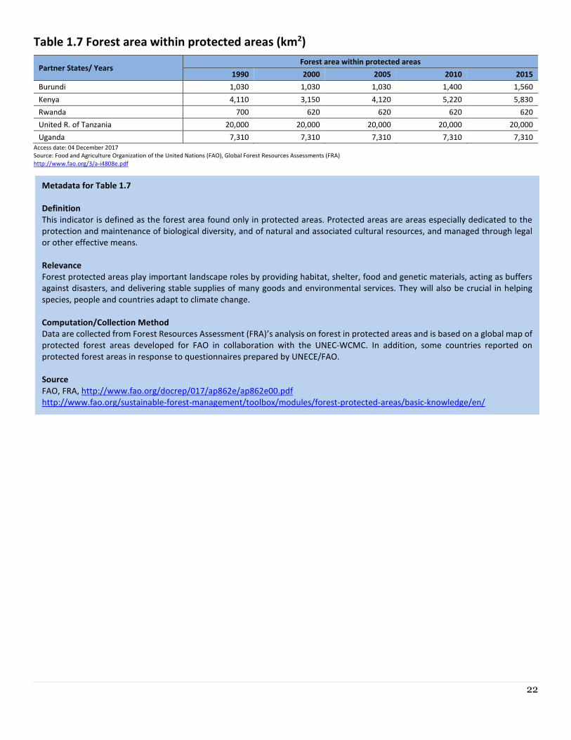
Table 1.7 Forest area within protected areas (km2)
Partner States/ Years Forest area within protected areas
1990 2000 2005 2010 2015
Burundi 1,030 1,030 1,030 1,400 1,560
Kenya 4,110 3,150 4,120 5,220 5,830
Rwanda 700 620 620 620 620
United R. of Tanzania 20,000 20,000 20,000 20,000 20,000
Uganda 7,310 7,310 7,310 7,310 7,310
Access date: 04 December 2017
Source: Food and Agriculture Organization of the United Nations (FAO), Global Forest Resources Assessments (FRA)
http://www.fao.org/3/a-i4808e.pdf
Metadata for Table 1.7
Definition
This indicator is defined as the forest area found only in protected areas. Protected areas are areas especially dedicated to the
protection and maintenance of biological diversity, and of natural and associated cultural resources, and managed through legal
or other effective means.
Relevance
Forest protected areas play important landscape roles by providing habitat, shelter, food and genetic materials, acting as buffers
against disasters, and delivering stable supplies of many goods and environmental services. They will also be crucial in helping
species, people and countries adapt to climate change.
Computation/Collection Method
Data are collected from Forest Resources Assessment (FRA)’s analysis on forest in protected areas and is based on a global map of
protected forest areas developed for FAO in collaboration with the UNEC-WCMC. In addition, some countries reported on
protected forest areas in response to questionnaires prepared by UNECE/FAO.
Source
FAO, FRA, http://www.fao.org/docrep/017/ap862e/ap862e00.pdf
http://www.fao.org/sustainable-forest-management/toolbox/modules/forest-protected-areas/basic-knowledge/en/
23
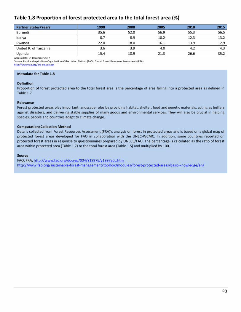
Table 1.8 Proportion of forest protected area to the total forest area (%)
Partner States/Years 1990 2000 2005 2010 2015
Burundi 35.6 52.0 56.9 55.3 56.5
Kenya 8.7 8.9 10.2 12.3 13.2
Rwanda 22.0 18.0 16.1 13.9 12.9
United R. of Tanzania 3.6 3.9 4.0 4.2 4.3
Uganda 15.4 18.9 21.3 26.6 35.2 Access date: 04 December 2017
Source: Food and Agriculture Organization of the United Nations (FAO), Global Forest Resources Assessments (FRA)
http://www.fao.org/3/a-i4808e.pdf
Metadata for Table 1.8
Definition
Proportion of forest protected area to the total forest area is the percentage of area falling into a protected area as defined in
Table 1.7.
Relevance
Forest protected areas play important landscape roles by providing habitat, shelter, food and genetic materials, acting as buffers
against disasters, and delivering stable supplies of many goods and environmental services. They will also be crucial in helping
species, people and countries adapt to climate change.
Computation/Collection Method
Data is collected from Forest Resources Assessment (FRA)’s analysis on forest in protected areas and is based on a global map of
protected forest areas developed for FAO in collaboration with the UNEC-WCMC. In addition, some countries reported on
protected forest areas in response to questionnaires prepared by UNECE/FAO. The percentage is calculated as the ratio of forest
area within protected area (Table 1.7) to the total forest area (Table 1.5) and multiplied by 100.
Source
FAO, FRA, http://www.fao.org/docrep/004/Y1997E/y1997e0c.htm
http://www.fao.org/sustainable-forest-management/toolbox/modules/forest-protected-areas/basic-knowledge/en/
24
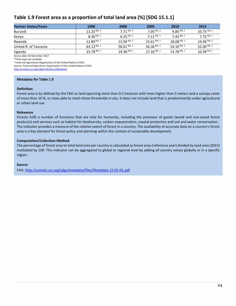
Table 1.9 Forest area as a proportion of total land area (%) [SDG 15.1.1]
Partner States/Years 1990 2000 2005 2010 2015
Burundi 11.25 NA, 1 7.71 NA, 1 7.05 NA, 1 9.85 NA, 1 10.75 NA, 1
Kenya 8.30 NA, 1 6.25 NA, 1 7.11 NA, 1 7.43 NA, 1 7.75 NA, 1
Rwanda 12.89 NA, 1 13.94 NA, 1 15.61 NA, 1 18.08 NA, 1 19.46 NA, 1
United R. of Tanzania 63.13 NA, 1 58.61 NA, 1 56.36 NA, 1 54.10 NA, 1 52.00 NA, 1
Uganda 23.78 NA, 1 19.36 NA, 1 17.16 NA, 1 13.78 NA, 1 10.39 NA, 1 Access date: 04 December 2017 NA Data type not available 1 Food and Agriculture Organization of the United Nations (FAO)
Source: Food and Agriculture Organization of the United Nations (FAO)
http://unstats.un.org/sdgs/indicators/database/
Metadata for Table 1.9
Definition
Forest area is by defined by the FAO as land spanning more than 0.5 hectares with trees higher than 5 meters and a canopy cover
of more than 10 %, or trees able to reach these thresholds in situ. It does not include land that is predominantly under agricultural
or urban land use.
Relevance
Forests fulfil a number of functions that are vital for humanity, including the provision of goods (wood and non-wood forest
products) and services such as habitat for biodiversity, carbon sequestration, coastal protection and soil and water conservation.
The indicator provides a measure of the relative extent of forest in a country. The availability of accurate data on a country's forest
area is a key element for forest policy and planning within the context of sustainable development.
Computation/Collection Method
The percentage of forest area to total land area per country is calculated as forest area (reference year) divided by land area (2015)
multiplied by 100. This indicator can be aggregated to global or regional level by adding all country values globally or in a specific
region.
Source
FAO, http://unstats.un.org/sdgs/metadata/files/Metadata-15-01-01.pdf
25
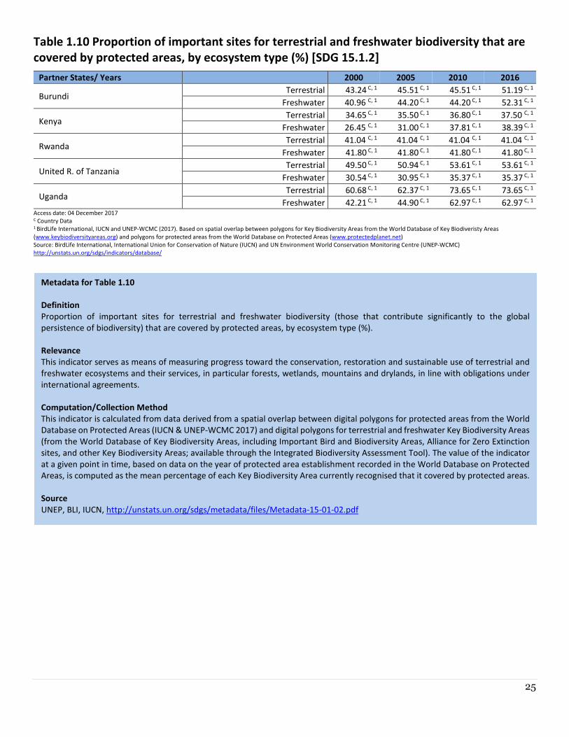
Table 1.10 Proportion of important sites for terrestrial and freshwater biodiversity that are
covered by protected areas, by ecosystem type (%) [SDG 15.1.2]
Partner States/ Years 2000 2005 2010 2016
Burundi Terrestrial 43.24 C, 1 45.51 C, 1 45.51 C, 1 51.19 C, 1
Freshwater 40.96 C, 1 44.20 C, 1 44.20 C, 1 52.31 C, 1
Kenya Terrestrial 34.65 C, 1 35.50 C, 1 36.80 C, 1 37.50 C, 1
Freshwater 26.45 C, 1 31.00 C, 1 37.81 C, 1 38.39 C, 1
Rwanda Terrestrial 41.04 C, 1 41.04 C, 1 41.04 C, 1 41.04 C, 1
Freshwater 41.80 C, 1 41.80 C, 1 41.80 C, 1 41.80 C, 1
United R. of Tanzania Terrestrial 49.50 C, 1 50.94 C, 1 53.61 C, 1 53.61 C, 1
Freshwater 30.54 C, 1 30.95 C, 1 35.37 C, 1 35.37 C, 1
Uganda Terrestrial 60.68 C, 1 62.37 C, 1 73.65 C, 1 73.65 C, 1
Freshwater 42.21 C, 1 44.90 C, 1 62.97 C, 1 62.97 C, 1 Access date: 04 December 2017 C Country Data 1 BirdLife International, IUCN and UNEP-WCMC (2017). Based on spatial overlap between polygons for Key Biodiversity Areas from the World Database of Key Biodiveristy Areas
(www.keybiodiversityareas.org) and polygons for protected areas from the World Database on Protected Areas (www.protectedplanet.net)
Source: BirdLife International, International Union for Conservation of Nature (IUCN) and UN Environment World Conservation Monitoring Centre (UNEP-WCMC)
http://unstats.un.org/sdgs/indicators/database/
Metadata for Table 1.10
Definition
Proportion of important sites for terrestrial and freshwater biodiversity (those that contribute significantly to the global
persistence of biodiversity) that are covered by protected areas, by ecosystem type (%).
Relevance
This indicator serves as means of measuring progress toward the conservation, restoration and sustainable use of terrestrial and
freshwater ecosystems and their services, in particular forests, wetlands, mountains and drylands, in line with obligations under
international agreements.
Computation/Collection Method
This indicator is calculated from data derived from a spatial overlap between digital polygons for protected areas from the World
Database on Protected Areas (IUCN & UNEP-WCMC 2017) and digital polygons for terrestrial and freshwater Key Biodiversity Areas
(from the World Database of Key Biodiversity Areas, including Important Bird and Biodiversity Areas, Alliance for Zero Extinction
sites, and other Key Biodiversity Areas; available through the Integrated Biodiversity Assessment Tool). The value of the indicator
at a given point in time, based on data on the year of protected area establishment recorded in the World Database on Protected
Areas, is computed as the mean percentage of each Key Biodiversity Area currently recognised that it covered by protected areas.
Source
UNEP, BLI, IUCN, http://unstats.un.org/sdgs/metadata/files/Metadata-15-01-02.pdf
26
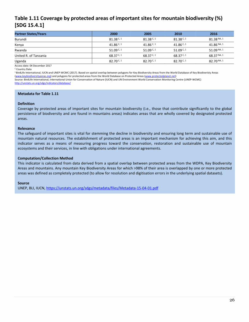
Table 1.11 Coverage by protected areas of important sites for mountain biodiversity (%)
[SDG 15.4.1]
Partner States/Years 2000 2005 2010 2016
Burundi 81.38 C, 1 81.38 C, 1 81.38 C, 1 81.38 NA, 1
Kenya 41.86 C, 1 41.86 C, 1 41.86 C, 1 41.86 NA, 1
Rwanda 51.09 C, 1 51.09 C, 1 51.09 C, 1 51.09 NA, 1
United R. of Tanzania 68.37 C, 1 68.37 C, 1 68.37 C, 1 68.37 NA, 1
Uganda 82.70 C, 1 82.70 C, 1 82.70 C, 1 82.70 NA, 1
Access date: 04 December 2017 C Country Data 1 BirdLife International, IUCN and UNEP-WCMC (2017). Based on spatial overlap between polygons for Key Biodiversity Areas from the World Database of Key Biodiveristy Areas
(www.keybiodiversityareas.org) and polygons for protected areas from the World Database on Protected Areas (www.protectedplanet.net)
Source: BirdLife International, International Union for Conservation of Nature (IUCN) and UN Environment World Conservation Monitoring Centre (UNEP-WCMC)
http://unstats.un.org/sdgs/indicators/database/
Metadata for Table 1.11
Definition
Coverage by protected areas of important sites for mountain biodiversity (i.e., those that contribute significantly to the global
persistence of biodiversity and are found in mountains areas) indicates areas that are wholly covered by designated protected
areas.
Relevance
The safeguard of important sites is vital for stemming the decline in biodiversity and ensuring long term and sustainable use of
mountain natural resources. The establishment of protected areas is an important mechanism for achieving this aim, and this
indicator serves as a means of measuring progress toward the conservation, restoration and sustainable use of mountain
ecosystems and their services, in line with obligations under international agreements.
Computation/Collection Method
This indicator is calculated from data derived from a spatial overlap between protected areas from the WDPA, Key Biodiversity
Areas and mountains. Any mountain Key Biodiversity Areas for which >98% of their area is overlapped by one or more protected
areas was defined as completely protected (to allow for resolution and digitisation errors in the underlying spatial datasets).
Source
UNEP, BLI, IUCN, https://unstats.un.org/sdgs/metadata/files/Metadata-15-04-01.pdf
27
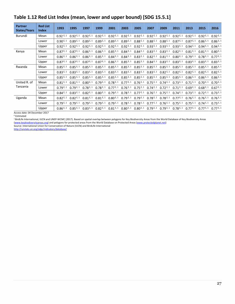
Table 1.12 Red List Index (mean, lower and upper bound) [SDG 15.5.1]
Partner
States/Years
Red List
Index 1993 1995 1997 1999 2001 2003 2005 2007 2009 2011 2013 2015 2016
Burundi Mean 0.92 E, 1 0.92 E, 1 0.92 E, 1 0.92 E, 1 0.92 E, 1 0.92 E, 1 0.92 E, 1 0.92 E, 1 0.92 E, 1 0.92 E, 1 0.92 E, 1 0.92 E, 1 0.92 E, 1
Lower 0.90 E, 1 0.89 E, 1 0.89 E, 1 0.89 E, 1 0.89 E, 1 0.89 E, 1 0.88 E, 1 0.88 E, 1 0.88 E, 1 0.87 E, 1 0.87 E, 1 0.86 E, 1 0.86 E, 1
Upper 0.92 E, 1 0.92 E, 1 0.92 E, 1 0.92 E, 1 0.92 E, 1 0.92 E, 1 0.92 E, 1 0.93 E, 1 0.93 E, 1 0.93 E, 1 0.94 E, 1 0.94 E, 1 0.94 E, 1
Kenya Mean 0.87 E, 1 0.87 E, 1 0.86 E, 1 0.86 E, 1 0.85 E, 1 0.84 E, 1 0.84 E, 1 0.83 E, 1 0.83 E, 1 0.82 E, 1 0.81 E, 1 0.81 E, 1 0.80 E, 1
Lower 0.86 E, 1 0.86 E, 1 0.86 E, 1 0.85 E, 1 0.84 E, 1 0.84 E, 1 0.83 E, 1 0.82 E, 1 0.81 E, 1 0.80 E, 1 0.79 E, 1 0.78 E, 1 0.77 E, 1
Upper 0.87 E, 1 0.87 E, 1 0.87 E, 1 0.87 E, 1 0.86 E, 1 0.85 E, 1 0.85 E, 1 0.84 E, 1 0.83 E, 1 0.83 E, 1 0.83 E, 1 0.83 E, 1 0.83 E, 1
Rwanda Mean 0.85 E, 1 0.85 E, 1 0.85 E, 1 0.85 E, 1 0.85 E, 1 0.85 E, 1 0.85 E, 1 0.85 E, 1 0.85 E, 1 0.85 E, 1 0.85 E, 1 0.85 E, 1 0.85 E, 1
Lower 0.83 E, 1 0.83 E, 1 0.83 E, 1 0.83 E, 1 0.83 E, 1 0.83 E, 1 0.83 E, 1 0.83 E, 1 0.82 E, 1 0.82 E, 1 0.82 E, 1 0.82 E, 1 0.82 E, 1
Upper 0.85 E, 1 0.85 E, 1 0.85 E, 1 0.85 E, 1 0.85 E, 1 0.85 E, 1 0.85 E, 1 0.85 E, 1 0.85 E, 1 0.85 E, 1 0.86 E, 1 0.86 E, 1 0.86 E, 1
United R. of
Tanzania
Mean 0.81 E, 1 0.81 E, 1 0.80 E, 1 0.79 E, 1 0.78 E, 1 0.77 E, 1 0.76 E, 1 0.75 E, 1 0.74 E, 1 0.73 E, 1 0.71 E, 1 0.70 E, 1 0.70 E, 1
Lower 0.79 E, 1 0.79 E, 1 0.78 E, 1 0.78 E, 1 0.77 E, 1 0.76 E, 1 0.75 E, 1 0.74 E, 1 0.72 E, 1 0.71 E, 1 0.69 E, 1 0.68 E, 1 0.67 E, 1
Upper 0.84 E, 1 0.83 E, 1 0.82 E, 1 0.80 E, 1 0.79 E, 1 0.78 E, 1 0.77 E, 1 0.76 E, 1 0.75 E, 1 0.74 E, 1 0.73 E, 1 0.72 E, 1 0.73 E, 1
Uganda Mean 0.82 E, 1 0.82 E, 1 0.81 E, 1 0.81 E, 1 0.80 E, 1 0.79 E, 1 0.79 E, 1 0.78 E, 1 0.78 E, 1 0.77 E, 1 0.76 E, 1 0.76 E, 1 0.76 E, 1
Lower 0.79 E, 1 0.79 E, 1 0.79 E, 1 0.79 E, 1 0.79 E, 1 0.78 E, 1 0.78 E, 1 0.77 E, 1 0.76 E, 1 0.75 E, 1 0.75 E, 1 0.74 E, 1 0.73 E, 1
Upper 0.86 E, 1 0.85 E, 1 0.83 E, 1 0.82 E, 1 0.81 E, 1 0.80 E, 1 0.80 E, 1 0.79 E, 1 0.79 E, 1 0.78 E, 1 0.77 E, 1 0.77 E, 1 0.77 E, 1
Access date: 04 December 2017 E Estimated 1 BirdLife International, IUCN and UNEP-WCMC (2017). Based on spatial overlap between polygons for Key Biodiversity Areas from the World Database of Key Biodiversity Areas
(www.keybiodiversityareas.org) and polygons for protected areas from the World Database on Protected Areas (www.protectedplanet.net)
Source: International Union for Conservation of Nature (IUCN) and BirdLife International
http://unstats.un.org/sdgs/indicators/database/
28
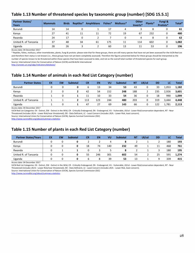
Table 1.13 Number of threatened species by taxonomic group (number) [SDG 15.5.1]
Partner States/
Years Mammals Birds Reptiles* Amphibians Fishes* Molluscs*
Other
Inverts* Plants*
Fungi &
Protists* Total*
Burundi 14 14 0 1 17 4 3 8 0 61
Kenya 27 41 11 11 72 19 67 232 0 480
Rwanda 24 17 0 2 7 0 4 8 0 62
United R. of Tanzania 37 48 34 61 175 11 114 602 0 1,082
Uganda 28 26 3 2 60 13 11 53 0 196
Access date: 04 December 2017
* Reptiles, fishes, molluscs, other invertebrates, plants, fungi & protists: please note that for these groups, there are still many species that have not yet been assessed for the IUCN Red List
and therefore their status is not known (i.e., these groups have not yet been completely assessed). Therefore the figures presented below for these groups should be interpreted as the
number of species known to be threatened within those species that have been assessed to date, and not as the overall total number of threatened species for each group.
Source: International Union for Conservation of Nature (IUCN) and BirdLife International
http://unstats.un.org/sdgs/indicators/database/
Table 1.14 Number of animals in each Red List Category (number)
Partner States EX EW Subtotal CR EN VU Subtotal NT LR/cd DD LC Total
Burundi 0 0 0 6 13 34 53 43 0 33 1,053 1,182
Kenya 2 0 2 42 54 152 248 188 2 235 2,926 3,601
Rwanda 1 0 1 11 10 33 54 36 0 18 990 1,099
United R. of Tanzania 1 1 2 113 123 244 480 203 0 319 3,444 4,448
Uganda 1 0 1 47 27 69 143 66 0 122 1,781 2,113
Access date: 04 December 2017
IUCN Red List Categories: EX - Extinct, EW - Extinct in the Wild, CR - Critically Endangered, EN - Endangered, VU - Vulnerable, LR/cd - Lower Risk/conservation dependent, NT - Near
Threatened (includes LR/nt - Lower Risk/near threatened), DD - Data Deficient, LC - Least Concern (includes LR/lc - Lower Risk, least concern).
Source: International Union for Conservation of Nature (IUCN), Species Survival Commission (SSC)
http://www.iucnredlist.org/about/summary-statistics
Table 1.15 Number of plants in each Red List Category (number)
Partner States/Years EX EW Subtotal CR EN VU Subtotal NT LR/cd DD LC Total
Burundi 0 0 0 2 2 4 8 2 1 2 180 193
Kenya 0 0 0 18 74 140 232 49 1 11 468 761
Rwanda 0 1 1 0 3 5 8 2 1 3 180 195
United R. of Tanzania 0 0 0 55 246 301 602 54 2 25 591 1,274
Uganda 0 0 0 6 8 39 53 13 1 9 339 415
Access date: 04 December 2017
IUCN Red List Categories: EX - Extinct, EW - Extinct in the Wild, CR - Critically Endangered, EN - Endangered, VU - Vulnerable, LR/cd - Lower Risk/conservation dependent, NT - Near
Threatened (includes LR/nt - Lower Risk/near threatened), DD - Data Deficient, LC - Least Concern (includes LR/lc - Lower Risk, least concern).
Source: International Union for Conservation of Nature (IUCN), Species Survival Commission (SSC)
http://www.iucnredlist.org/about/summary-statistics
29
Metadata for Table 1.12, Table 1.13, Table 1.14 and Table 1.15
Definition
The Red List Index measures changes in aggregation extinction risk across group of species. It is based on changes in the number
of species in each category of extinction risk on the IUCN Red List of Threatened Species (IUCN 2015) and is expressed as changes
in an index ranging from 0 to 1. 1 is defined as ‘Least Concern’ to 0 ‘All species are categorized as ‘Extinct’.
Relevance
This index allows comparison between sets of species in both how treated they are on average and the rate at which risk changes
over time. This indicator serves as a means of measuring progress toward the conservation, restoration and sustainable use of
mountain ecosystems and their services, in line with obligations under international agreements.
A downward trend in the Red List Index over time means that the expected rate of future species extinctions is worsening. An
upward trend means that the expected rate of species extinctions is abating and a horizontal line means that the expected rate of
species extinctions is remaining the same, although in each of these cases it does not mean that biodiversity loss has stopped. A
Red List Index value of 1 would indicate that biodiversity loss has been halted.
Computation/Collection Method
This index is calculated at a point in time by multiplying the number of species in each Red List Category by a weight (ranging from
1 for ‘Near Threatened’ to 5 for ‘Extinct’ and ‘Extinct in the Wild’) and summing these values. This is then divided by a maximum
threat score which is the total number of species multiplied by the weight assigned to the “Extinct” category. This final value is
subtracted from 1 to give the Red List Index value.
Table 1.12 presents values calculated for December 2016. Table 1.13 shows the number of threatened species assessed as Critically
Endangered (CR), Endangered (EN), or Vulnerable (VU) are referred to as "threatened" species. This classification is based according
to the Red List Index, status and population size of the taxon at a global level, ecological traits, economics, cultural value, practicality
of recovery action and more. For Reptiles, fishes, molluscs, other invertebrates, plants, fungi & protists there are still many species
that have not yet been assessed for the IUCN Red List and therefore their status is not known (i.e., these groups have not yet been
completely assessed).
Numbers in Table 1.14 and Table 1.15 are evaluated according to population size reduction, geographic range, small population
size and decline, very small or restricted population and quantitative analysis. Some taxonomic groups are better known than
others therefore proportion of threatened species is only reported for the more completely evaluated groups where >80% of
species have been evaluated.
Source
IUCN, BLI, https://unstats.un.org/sdgs/metadata/files/Metadata-15-05-01.pdf
30
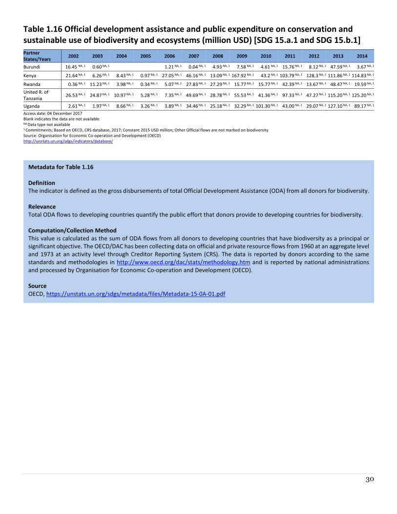
Table 1.16 Official development assistance and public expenditure on conservation and
sustainable use of biodiversity and ecosystems (million USD) [SDG 15.a.1 and SDG 15.b.1]
Partner
States/Years 2002 2003 2004 2005 2006 2007 2008 2009 2010 2011 2012 2013 2014
Burundi 16.45 NA, 1 0.60 NA, 1 1.21 NA, 1 0.04 NA, 1 4.93 NA, 1 7.58 NA, 1 4.61 NA, 1 15.76 NA, 1 8.12 NA, 1 47.59 NA, 1 3.67 NA, 1
Kenya 21.64 NA, 1 6.26 NA, 1 8.43 NA, 1 0.97 NA, 1 27.05 NA, 1 46.16 NA, 1 13.09 NA, 1 167.92 NA, 1 43.2 NA, 1 103.79 NA, 1 128.3 NA, 1 111.86 NA, 1 114.83 NA, 1
Rwanda 0.36 NA, 1 11.23 NA, 1 3.98 NA, 1 0.34 NA, 1 5.07 NA, 1 27.83 NA, 1 27.29 NA, 1 15.77 NA, 1 15.77 NA, 1 42.39 NA, 1 13.67 NA, 1 48.47 NA, 1 19.59 NA, 1
United R. of
Tanzania 26.53 NA, 1 24.87 NA, 1 10.97 NA, 1 5.28 NA, 1 7.35 NA, 1 49.69 NA, 1 28.78 NA, 1 55.53 NA, 1 41.36 NA, 1 97.33 NA, 1 47.27 NA, 1 115.20 NA, 1 125.20 NA, 1
Uganda 2.61 NA, 1 1.97 NA, 1 8.66 NA, 1 3.26 NA, 1 3.89 NA, 1 34.46 NA, 1 25.18 NA, 1 32.29 NA, 1 101.30 NA, 1 43.00 NA, 1 29.07 NA, 1 127.10 NA, 1 89.17 NA, 1
Access date: 04 December 2017
Blank indicates the data are not available NA Data type not available 1 Commitments; Based on OECD, CRS database, 2017; Constant 2015 USD million; Other Official flows are not marked on biodiversity
Source: Organisation for Economic Co-operation and Development (OECD)
http://unstats.un.org/sdgs/indicators/database/
Metadata for Table 1.16
Definition
The indicator is defined as the gross disbursements of total Official Development Assistance (ODA) from all donors for biodiversity.
Relevance
Total ODA flows to developing countries quantify the public effort that donors provide to developing countries for biodiversity.
Computation/Collection Method
This value is calculated as the sum of ODA flows from all donors to developing countries that have biodiversity as a principal or
significant objective. The OECD/DAC has been collecting data on official and private resource flows from 1960 at an aggregate level
and 1973 at an activity level through Creditor Reporting System (CRS). The data is reported by donors according to the same
standards and methodologies in http://www.oecd.org/dac/stats/methodology.htm and is reported by national administrations
and processed by Organisation for Economic Co-operation and Development (OECD).
Source
OECD, https://unstats.un.org/sdgs/metadata/files/Metadata-15-0A-01.pdf
31
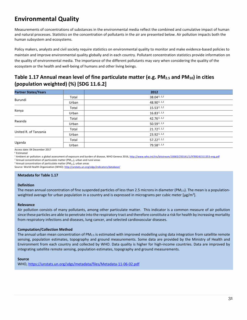
Environmental Quality
Measurements of concentrations of substances in the environmental media reflect the combined and cumulative impact of human
and natural processes. Statistics on the concentration of pollutants in the air are presented below. Air pollution impacts both the
human subsystem and ecosystems.
Policy makers, analysts and civil society require statistics on environmental quality to monitor and make evidence-based policies to
maintain and improve environmental quality globally and in each country. Pollutant concentration statistics provide information on
the quality of environmental media. The importance of the different pollutants may vary when considering the quality of the
ecosystem or the health and well-being of humans and other living beings.
Table 1.17 Annual mean level of fine particulate matter (e.g. PM2.5 and PM10) in cities
(population weighted) (%) [SDG 11.6.2]
Partner States/Years 2012
Burundi Total 38.04 E, 1,2
Urban 48.90 E, 1,3
Kenya Total 15.53 E, 1,2
Urban 16.83 E, 1,3
Rwanda Total 42.76 E, 1,2
Urban 50.59 E, 1,3
United R. of Tanzania Total 21.72 E, 1,2
Urban 23.92 E, 1,3
Uganda Total 57.22 E, 1,2
Urban 79.58 E, 1,3 Access date: 04 December 2017 E Estimated 1
Ambient air pollution: a global assessment of exposure and burden of disease, WHO Geneva 2016, http://www.who.int/iris/bitstream/10665/250141/1/9789241511353-eng.pdf 2 Annual concentration of particulate matter (PM2.5), urban and rural areas 3 Annual concentration of particulate matter (PM2.5), urban areas
Source: World Health Organization (WHO): http://unstats.un.org/sdgs/indicators/database/
Metadata for Table 1.17
Definition
The mean annual concentration of fine suspended particles of less than 2.5 microns in diameter (PM2.5). The mean is a population-
weighted average for urban population in a country and is expressed in micrograms per cubic meter [µg/m3].
Relevance
Air pollution consists of many pollutants, among other particulate matter. This indicator is a common measure of air pollution
since these particles are able to penetrate into the respiratory tract and therefore constitute a risk for health by increasing mortality
from respiratory infections and diseases, lung cancer, and selected cardiovascular diseases.
Computation/Collection Method
The annual urban mean concentration of PM2.5 is estimated with improved modelling using data integration from satellite remote
sensing, population estimates, topography and ground measurements. Some data are provided by the Ministry of Health and
Environment from each country and collected by WHO. Data quality is higher for high-income countries. Data are improved by
integrating satellite remote sensing, population estimates, topography and ground measurements.
Source
WHO, https://unstats.un.org/sdgs/metadata/files/Metadata-11-06-02.pdf
32
Chapter 2 Environmental Resources and their
Use
33
CHAPTER 2 ENVIRONMENTAL RESOURCES AND THEIR USE
Environmental resources (or assets, as they are referred to in the System of Environmental-Economic Accounting Central
Framework (SEEA-CF)) are the naturally occurring living and non-living components of the earth, together constituting the
biophysical environment, which may provide benefits to humanity. Environmental resources include natural resources,
such as subsoil resources (mineral and energy), biological resources and water resources, and land. They may be naturally
renewable (e.g., fish, timber or water) or non-renewable (e.g., minerals).
They are important in every aspect of human activity such as shelter, food, health care, infrastructure, communications,
transportation, defence and more. Thus, statistics of quality and availability of environmental resources are needed for
policy makers to make informed decisions, especially to avoid the shortage or restriction of their use and availability. The
main focus is the measure of stock variability over time, space and their use for production and consumption.
Mineral Resources Minerals are elements or compounds composed of natural occurring inorganic materials in or on the earth’s crust. The
family is composed of metal ores (including precious metals and rare earths); non-metallic minerals such as coal, oil, gas,
stone, sand and clay; chemical and fertilizer minerals; salt; and various other minerals such as gemstones, abrasive
minerals, graphite, asphalt, natural solid bitumen, quartz and mica.
Mineral resources are not renewable so their depletion reduces their availability in the environment over time. The scale
of their extraction can determine the amount of stress placed on the environment.
34
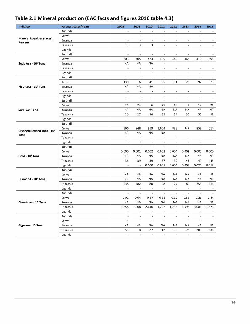
Table 2.1 Mineral production (EAC facts and figures 2016 table 4.3)
Indicator Partner States/Years 2008 2009 2010 2011 2012 2013 2014 2015
Mineral Royalties (taxes)
Percent
Burundi - - - - - - - -
Kenya - - - - - - - -
Rwanda - - - - - - - -
Tanzania 3 3 3 - - - - -
Uganda - - - - - - - -
Soda Ash - 103 Tons
Burundi - - - - - - - -
Kenya 503 405 474 499 449 468 410 295
Rwanda NA NA NA -
Tanzania - - - - - - - -
Uganda - - - - - - - -
Fluorspar - 103 Tons
Burundi - - - - - - - -
Kenya 130 6 41 95 91 78 97 70
Rwanda NA NA NA -
Tanzania - - - - - - - -
Uganda - - - - - - - -
Salt - 103 Tons
Burundi - - - - - - - -
Kenya 24 24 6 25 10 9 19 21
Rwanda NA NA NA NA NA NA NA NA
Tanzania 26 27 34 32 34 36 55 92
Uganda - - - - - - - -
Crushed Refined soda - 103
Tons
Burundi - - - - - - - -
Kenya 866 948 959 1,054 883 947 852 614
Rwanda NA NA NA NA
Tanzania - - - - - - - -
Uganda - - - - - - - -
Gold - 103 Tons
Burundi - - - - - - - -
Kenya 0.000 0.001 0.002 0.002 0.004 0.002 0.000 0.000
Rwanda NA NA NA NA NA NA NA NA
Tanzania 36 39 39 37 39 43 40 46
Uganda - - 0.000 0.001 0.004 0.005 0.024 0.013
Diamond - 103 Tons
Burundi - - - - - - - -
Kenya NA NA NA NA NA NA NA NA
Rwanda NA NA NA NA NA NA NA NA
Tanzania 238 182 80 28 127 180 253 216
Uganda - - - - - - - -
Gemstone - 103Tons
Burundi - - - - - - - -
Kenya 0.02 0.04 0.17 0.31 0.12 0.56 0.25 0.44
Rwanda NA NA NA NA NA NA NA NA
Tanzania 1,858 1,068 2,646 1,242 1,238 1,692 3,084 1,873
Uganda - - - - - - - -
Gypsum - 103Tons
Burundi - - - - - - - -
Kenya 5 - - - - - - -
Rwanda NA NA NA NA NA NA NA NA
Tanzania 56 8 27 12 92 172 200 236
Uganda - - - - - - - -
35
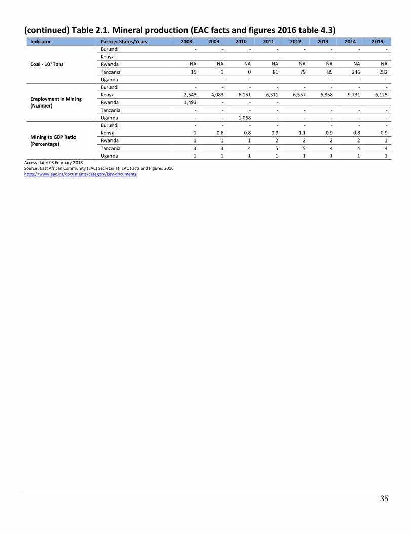
(continued) Table 2.1. Mineral production (EAC facts and figures 2016 table 4.3) Indicator Partner States/Years 2008 2009 2010 2011 2012 2013 2014 2015
Coal - 103 Tons
Burundi - - - - - - - -
Kenya - - - - - - - -
Rwanda NA NA NA NA NA NA NA NA
Tanzania 15 1 0 81 79 85 246 282
Uganda - - - - - - - -
Employment in Mining
(Number)
Burundi - - - - - - - -
Kenya 2,543 4,083 6,151 6,311 6,557 6,858 9,731 6,125
Rwanda 1,493 - - -
Tanzania - - - - - - - -
Uganda - - 1,068 - - - - -
Mining to GDP Ratio
(Percentage)
Burundi - - - - - - - -
Kenya 1 0.6 0.8 0.9 1.1 0.9 0.8 0.9
Rwanda 1 1 1 2 2 2 2 1
Tanzania 3 3 4 5 5 4 4 4
Uganda 1 1 1 1 1 1 1 1
Access date: 08 February 2018
Source: East African Community (EAC) Secretariat, EAC Facts and Figures 2016
https://www.eac.int/documents/category/key-documents
36
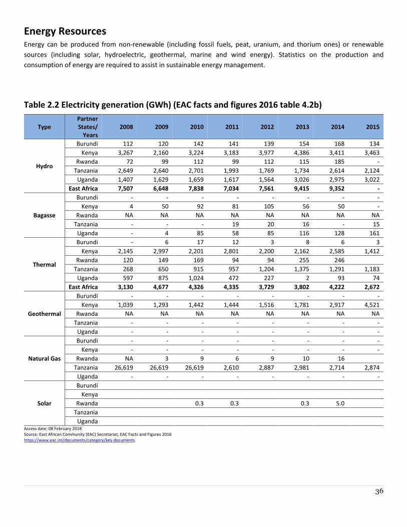
Energy Resources Energy can be produced from non-renewable (including fossil fuels, peat, uranium, and thorium ones) or renewable
sources (including solar, hydroelectric, geothermal, marine and wind energy). Statistics on the production and
consumption of energy are required to assist in sustainable energy management.
Table 2.2 Electricity generation (GWh) (EAC facts and figures 2016 table 4.2b)
Type
Partner
States/
Years
2008 2009 2010 2011 2012 2013 2014 2015
Hydro
Burundi 112 120 142 141 139 154 168 134
Kenya 3,267 2,160 3,224 3,183 3,977 4,386 3,411 3,463
Rwanda 72 99 112 99 112 115 185 -
Tanzania 2,649 2,640 2,701 1,993 1,769 1,734 2,614 2,124
Uganda 1,407 1,629 1,659 1,617 1,564 3,026 2,975 3,022
East Africa 7,507 6,648 7,838 7,034 7,561 9,415 9,352 -
Bagasse
Burundi - - - - - - - -
Kenya 4 50 92 81 105 56 50 -
Rwanda NA NA NA NA NA NA NA NA
Tanzania - - - 19 20 16 - 15
Uganda - 4 85 58 85 116 128 161
Thermal
Burundi - 6 17 12 3 8 6 3
Kenya 2,145 2,997 2,201 2,801 2,200 2,162 2,585 1,412
Rwanda 120 149 169 94 94 255 246
Tanzania 268 650 915 957 1,204 1,375 1,291 1,183
Uganda 597 875 1,024 472 227 2 93 74
East Africa 3,130 4,677 4,326 4,335 3,729 3,802 4,222 2,672
Geothermal
Burundi - - - - - - - -
Kenya 1,039 1,293 1,442 1,444 1,516 1,781 2,917 4,521
Rwanda NA NA NA NA NA NA NA NA
Tanzania - - - - - - - -
Uganda - - - - - - - -
Natural Gas
Burundi - - - - - - - -
Kenya - - - - - - - -
Rwanda NA 3 9 6 9 10 16
Tanzania 26,619 26,619 26,619 2,610 2,887 2,981 2,714 2,874
Uganda - - - - - - - -
Solar
Burundi
Kenya
Rwanda 0.3 0.3 0.3 5.0
Tanzania
Uganda Access date: 08 February 2018
Source: East African Community (EAC) Secretariat, EAC Facts and Figures 2016
https://www.eac.int/documents/category/key-documents
37
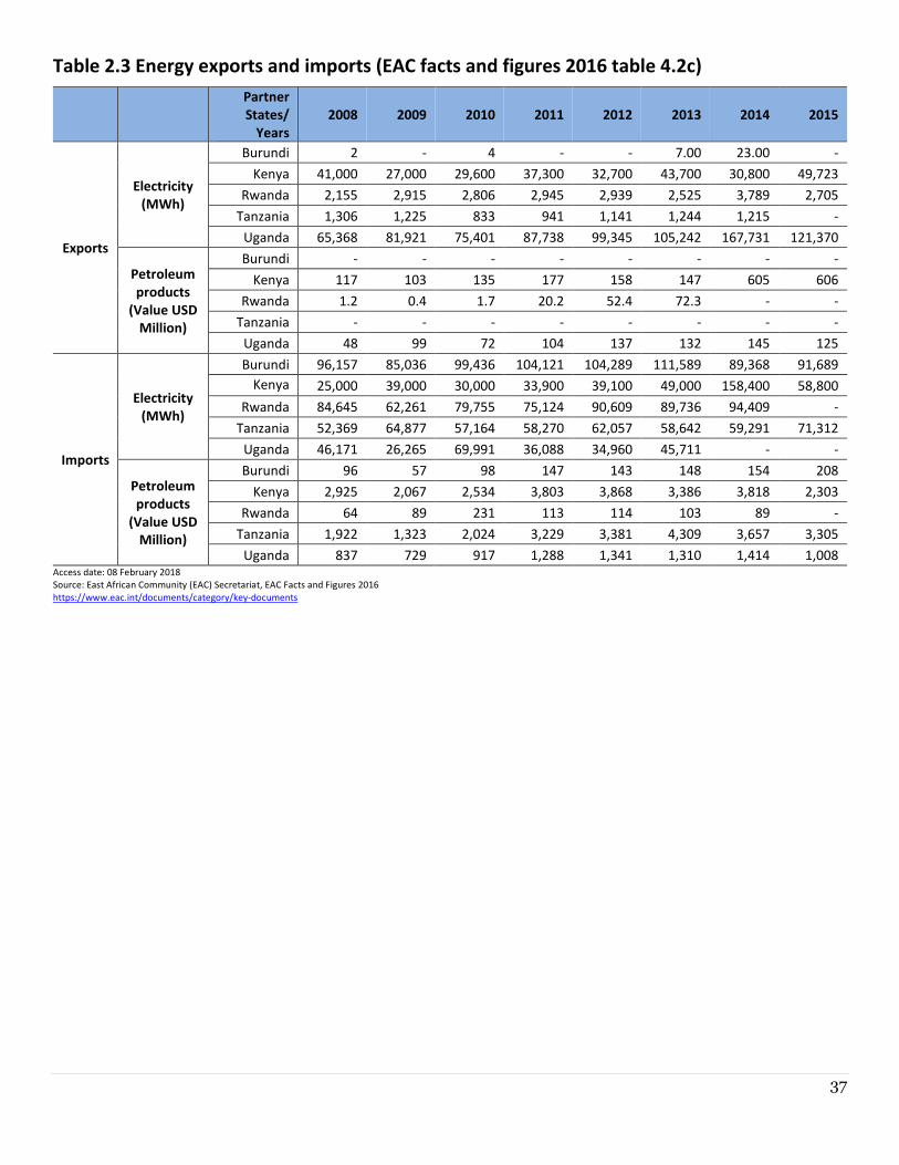
Table 2.3 Energy exports and imports (EAC facts and figures 2016 table 4.2c)
Partner
States/
Years
2008 2009 2010 2011 2012 2013 2014 2015
Exports
Electricity
(MWh)
Burundi 2 - 4 - - 7.00 23.00 -
Kenya 41,000 27,000 29,600 37,300 32,700 43,700 30,800 49,723
Rwanda 2,155 2,915 2,806 2,945 2,939 2,525 3,789 2,705
Tanzania 1,306 1,225 833 941 1,141 1,244 1,215 -
Uganda 65,368 81,921 75,401 87,738 99,345 105,242 167,731 121,370
Petroleum
products
(Value USD
Million)
Burundi - - - - - - - -
Kenya 117 103 135 177 158 147 605 606
Rwanda 1.2 0.4 1.7 20.2 52.4 72.3 - -
Tanzania - - - - - - - -
Uganda 48 99 72 104 137 132 145 125
Imports
Electricity
(MWh)
Burundi 96,157 85,036 99,436 104,121 104,289 111,589 89,368 91,689
Kenya
25,000 39,000 30,000 33,900 39,100 49,000 158,400 58,800
Rwanda 84,645 62,261 79,755 75,124 90,609 89,736 94,409 -
Tanzania 52,369 64,877 57,164 58,270 62,057 58,642 59,291 71,312
Uganda 46,171 26,265 69,991 36,088 34,960 45,711 - -
Petroleum
products
(Value USD
Million)
Burundi 96 57 98 147 143 148 154 208
Kenya 2,925 2,067 2,534 3,803 3,868 3,386 3,818 2,303
Rwanda 64 89 231 113 114 103 89 -
Tanzania 1,922 1,323 2,024 3,229 3,381 4,309 3,657 3,305
Uganda 837 729 917 1,288 1,341 1,310 1,414 1,008 Access date: 08 February 2018
Source: East African Community (EAC) Secretariat, EAC Facts and Figures 2016
https://www.eac.int/documents/category/key-documents
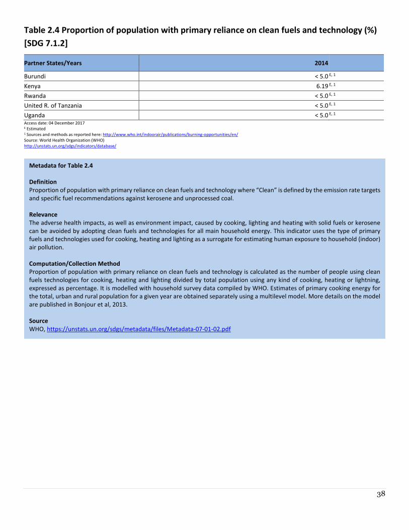
38
Table 2.4 Proportion of population with primary reliance on clean fuels and technology (%)
[SDG 7.1.2]
Partner States/Years 2014
Burundi < 5.0 E, 1
Kenya 6.19 E, 1
Rwanda < 5.0 E, 1
United R. of Tanzania < 5.0 E, 1
Uganda < 5.0 E, 1 Access date: 04 December 2017 E Estimated 1 Sources and methods as reported here: http://www.who.int/indoorair/publications/burning-opportunities/en/
Source: World Health Organization (WHO)
http://unstats.un.org/sdgs/indicators/database/
Metadata for Table 2.4
Definition
Proportion of population with primary reliance on clean fuels and technology where “Clean” is defined by the emission rate targets
and specific fuel recommendations against kerosene and unprocessed coal.
Relevance
The adverse health impacts, as well as environment impact, caused by cooking, lighting and heating with solid fuels or kerosene
can be avoided by adopting clean fuels and technologies for all main household energy. This indicator uses the type of primary
fuels and technologies used for cooking, heating and lighting as a surrogate for estimating human exposure to household (indoor)
air pollution.
Computation/Collection Method
Proportion of population with primary reliance on clean fuels and technology is calculated as the number of people using clean
fuels technologies for cooking, heating and lighting divided by total population using any kind of cooking, heating or lightning,
expressed as percentage. It is modelled with household survey data compiled by WHO. Estimates of primary cooking energy for
the total, urban and rural population for a given year are obtained separately using a multilevel model. More details on the model
are published in Bonjour et al, 2013.
Source
WHO, https://unstats.un.org/sdgs/metadata/files/Metadata-07-01-02.pdf
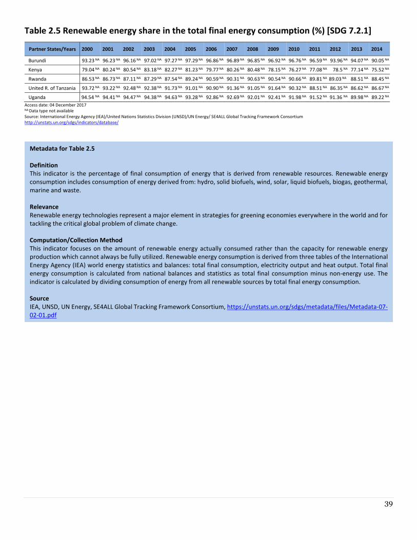
39
Table 2.5 Renewable energy share in the total final energy consumption (%) [SDG 7.2.1]
Partner States/Years 2000 NA 2001 NA 2002 NA 2003 NA 2004 NA 2005 NA 2006 NA 2007 NA 2008 NA 2009 NA 2010 NA 2011 NA 2012 NA 2013NA 2014 NA
Burundi 93.23 NA 96.23 NA 96.16 NA 97.02 NA 97.27 NA 97.29 NA 96.86 NA 96.89 NA 96.85 NA 96.92 NA 96.76 NA 96.59 NA 93.96 NA 94.07 NA 90.05 NA
Kenya 79.04 NA 80.24 NA 80.54 NA 83.18 NA 82.27 NA 81.23 NA 79.77 NA 80.26 NA 80.48 NA 78.15 NA 76.27 NA 77.08 NA 78.5 NA 77.14 NA 75.52 NA
Rwanda 86.53 NA 86.73 NA 87.11 NA 87.29 NA 87.54 NA 89.24 NA 90.59 NA 90.31 NA 90.63 NA 90.54 NA 90.66 NA 89.81 NA 89.03 NA 88.51 NA 88.45 NA
United R. of Tanzania 93.72 NA 93.22 NA 92.48 NA 92.38 NA 91.73 NA 91.01 NA 90.90 NA 91.36 NA 91.05 NA 91.64 NA 90.32 NA 88.51 NA 86.35 NA 86.62 NA 86.67 NA
Uganda 94.54 NA 94.41 NA 94.47 NA 94.38 NA 94.63 NA 93.28 NA 92.86 NA 92.69 NA 92.01 NA 92.41 NA 91.98 NA 91.52 NA 91.36 NA 89.98 NA 89.22 NA
Access date: 04 December 2017 NA Data type not available
Source: International Energy Agency (IEA)/United Nations Statistics Division (UNSD)/UN Energy/ SE4ALL Global Tracking Framework Consortium
http://unstats.un.org/sdgs/indicators/database/
Metadata for Table 2.5
Definition
This indicator is the percentage of final consumption of energy that is derived from renewable resources. Renewable energy
consumption includes consumption of energy derived from: hydro, solid biofuels, wind, solar, liquid biofuels, biogas, geothermal,
marine and waste.
Relevance
Renewable energy technologies represent a major element in strategies for greening economies everywhere in the world and for
tackling the critical global problem of climate change.
Computation/Collection Method
This indicator focuses on the amount of renewable energy actually consumed rather than the capacity for renewable energy
production which cannot always be fully utilized. Renewable energy consumption is derived from three tables of the International
Energy Agency (IEA) world energy statistics and balances: total final consumption, electricity output and heat output. Total final
energy consumption is calculated from national balances and statistics as total final consumption minus non-energy use. The
indicator is calculated by dividing consumption of energy from all renewable sources by total final energy consumption.
Source
IEA, UNSD, UN Energy, SE4ALL Global Tracking Framework Consortium, https://unstats.un.org/sdgs/metadata/files/Metadata-07-
02-01.pdf
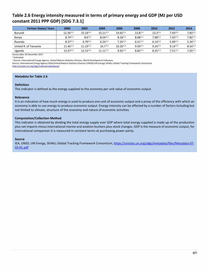
40
Table 2.6 Energy intensity measured in terms of primary energy and GDP (MJ per USD
constant 2011 PPP GDP) [SDG 7.3.1]
Partner States/ Years 2000 2002 2004 2006 2008 2010 2012 2014
Burundi 11.34 E,1 15.19 E,1 15.11 E,1 14.65 E,1 13.8 E,1 13.3 E,1 7.93 E,1 7.83 E,1
Kenya 8.74 E,1 8.6 E,1 8.54 E,1 8.18 E,1 8.08 E,1 7.98 E,1 7.43 E,1 7.82 E,1
Rwanda 8.37 E,1 6.79 E,1 6.24 E,1 7.24 E,1 6.51 E,1 6.14 E,1 5.69 E,1 5.34 E,1
United R. of Tanzania 11.46 E,1 11.19 E,1 10.7 E,1 10.26 E,1 9.59 E,1 9.24 E,1 9.14 E,1 8.54 E,1
Uganda 13.37 E,1 12.13 E,1 11.11 E,1 9.92 E,1 8.82 E,1 8.25 E,1 7.51 E,1 7.03 E,1
Access date: 04 December 2017 E Estimated 1 Source: International Energy Agency, United Nations Statistics Division, World Development Indicators
Source: International Energy Agency (IEA)/United Nations Statistics Division (UNSD)/UN Energy/ SE4ALL Global Tracking Framework Consortium
http://unstats.un.org/sdgs/indicators/database/
Metadata for Table 2.6
Definition
This indicator is defined as the energy supplied to the economy per unit value of economic output.
Relevance
It is an indication of how much energy is used to produce one unit of economic output and a proxy of the efficiency with which an
economy is able to use energy to produce economic output. Energy intensity can be affected by a number of factors including but
not limited to climate, structure of the economy and nature of economic activities.
Computation/Collection Method
This indicator is obtained by dividing the total energy supply over GDP where total energy supplied is made up of the production
plus net imports minus international marine and aviation bunkers plus-stock changes. GDP is the measure of economic output, for
international comparison it is measured in constant terms at purchasing power parity.
Source
IEA, UNSD, UN Energy, SE4ALL Global Tracking Framework Consortium, https://unstats.un.org/sdgs/metadata/files/Metadata-07-
03-01.pdf
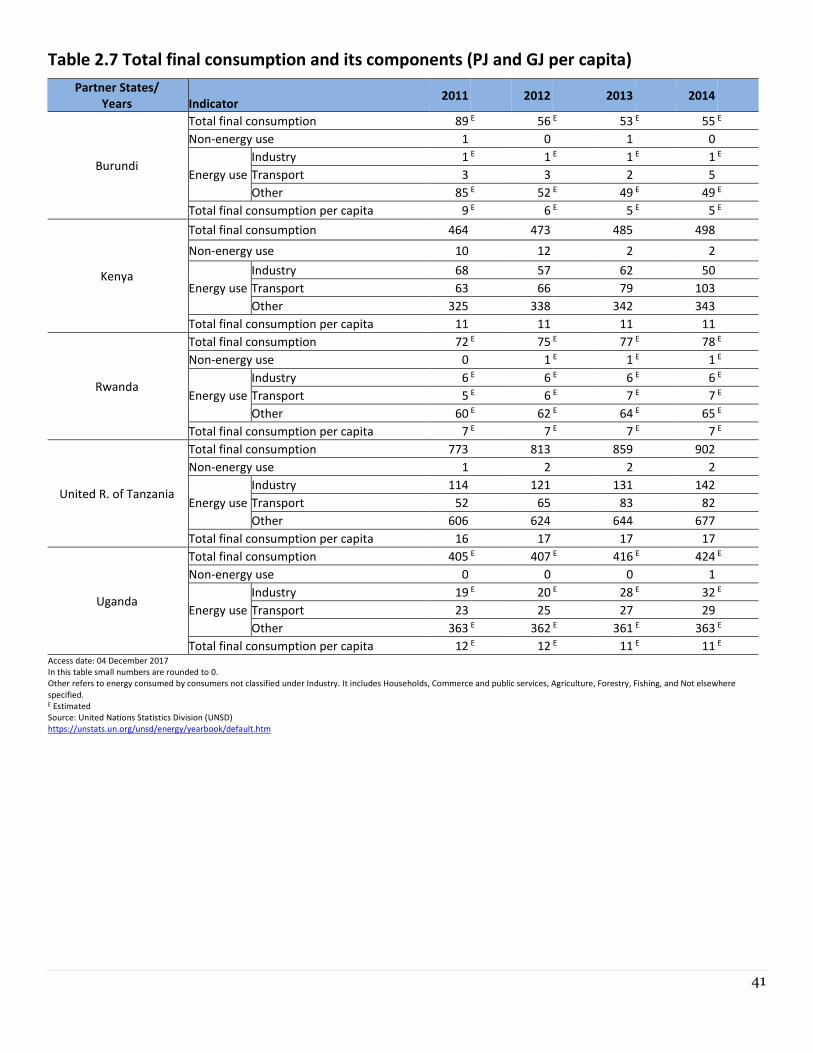
41
Table 2.7 Total final consumption and its components (PJ and GJ per capita)
Partner States/
Years
Indicator 2011 2012 2013 2014
Burundi
Total final consumption 89 E 56 E 53 E 55 E
Non-energy use 1 0 1 0
Energy use
Industry 1 E 1 E 1 E 1 E
Transport 3 3 2 5
Other 85 E 52 E 49 E 49 E
Total final consumption per capita 9 E 6 E 5 E 5 E
Kenya
Total final consumption 464 473 485 498
Non-energy use 10 12 2 2
Energy use
Industry 68 57 62 50
Transport 63 66 79 103
Other 325 338 342 343
Total final consumption per capita 11 11 11 11
Rwanda
Total final consumption 72 E 75 E 77 E 78 E
Non-energy use 0 1 E 1 E 1 E
Energy use
Industry 6 E 6 E 6 E 6 E
Transport 5 E 6 E 7 E 7 E
Other 60 E 62 E 64 E 65 E
Total final consumption per capita 7 E 7 E 7 E 7 E
United R. of Tanzania
Total final consumption 773 813 859 902
Non-energy use 1 2 2 2
Energy use
Industry 114 121 131 142
Transport 52 65 83 82
Other 606 624 644 677
Total final consumption per capita 16 17 17 17
Uganda
Total final consumption 405 E 407 E 416 E 424 E
Non-energy use 0 0 0 1
Energy use
Industry 19 E 20 E 28 E 32 E
Transport 23 25 27 29
Other 363 E 362 E 361 E 363 E
Total final consumption per capita 12 E 12 E 11 E 11 E
Access date: 04 December 2017
In this table small numbers are rounded to 0.
Other refers to energy consumed by consumers not classified under Industry. It includes Households, Commerce and public services, Agriculture, Forestry, Fishing, and Not elsewhere
specified. E Estimated Source: United Nations Statistics Division (UNSD) https://unstats.un.org/unsd/energy/yearbook/default.htm
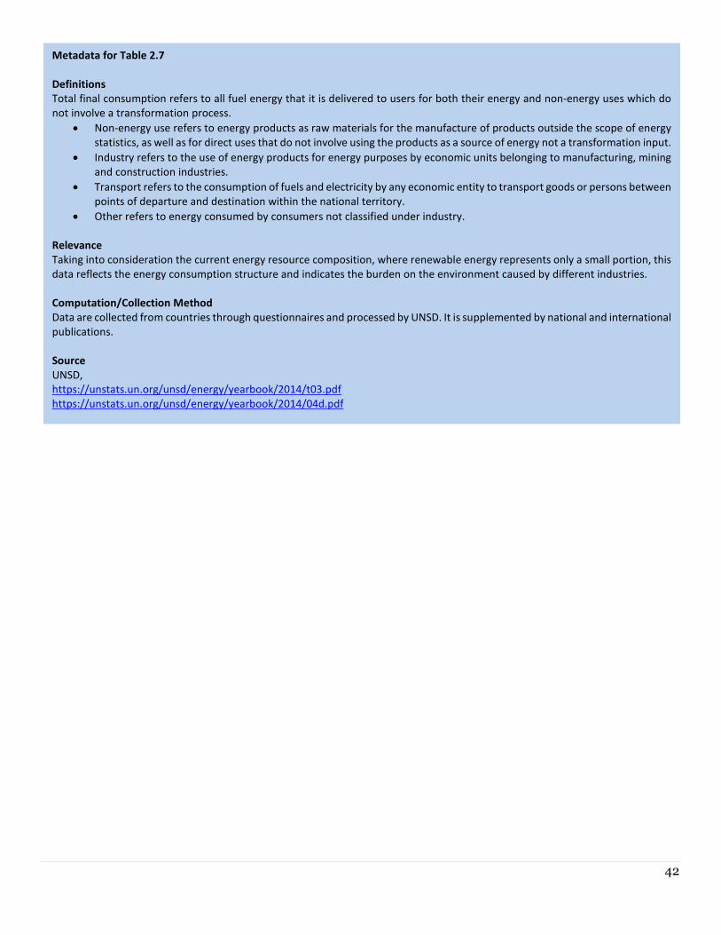
42
Metadata for Table 2.7
Definitions
Total final consumption refers to all fuel energy that it is delivered to users for both their energy and non-energy uses which do
not involve a transformation process.
• Non-energy use refers to energy products as raw materials for the manufacture of products outside the scope of energy
statistics, as well as for direct uses that do not involve using the products as a source of energy not a transformation input.
• Industry refers to the use of energy products for energy purposes by economic units belonging to manufacturing, mining
and construction industries.
• Transport refers to the consumption of fuels and electricity by any economic entity to transport goods or persons between
points of departure and destination within the national territory.
• Other refers to energy consumed by consumers not classified under industry.
Relevance
Taking into consideration the current energy resource composition, where renewable energy represents only a small portion, this
data reflects the energy consumption structure and indicates the burden on the environment caused by different industries.
Computation/Collection Method
Data are collected from countries through questionnaires and processed by UNSD. It is supplemented by national and international
publications.
Source
UNSD,
https://unstats.un.org/unsd/energy/yearbook/2014/t03.pdf
https://unstats.un.org/unsd/energy/yearbook/2014/04d.pdf
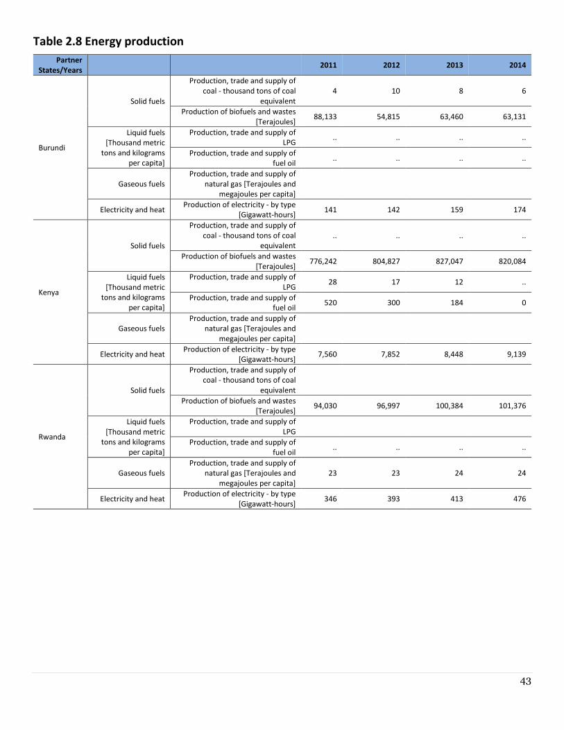
43
Table 2.8 Energy production
Partner
States/Years 2011 2012 2013 2014
Burundi
Solid fuels
Production, trade and supply of
coal - thousand tons of coal
equivalent
4 10 8 6
Production of biofuels and wastes
[Terajoules] 88,133 54,815 63,460 63,131
Liquid fuels
[Thousand metric
tons and kilograms
per capita]
Production, trade and supply of
LPG .. .. .. ..
Production, trade and supply of
fuel oil .. .. .. ..
Gaseous fuels
Production, trade and supply of
natural gas [Terajoules and
megajoules per capita]
Electricity and heat Production of electricity - by type
[Gigawatt-hours] 141 142 159 174
Kenya
Solid fuels
Production, trade and supply of
coal - thousand tons of coal
equivalent
.. .. .. ..
Production of biofuels and wastes
[Terajoules] 776,242 804,827 827,047 820,084
Liquid fuels
[Thousand metric
tons and kilograms
per capita]
Production, trade and supply of
LPG 28 17 12 ..
Production, trade and supply of
fuel oil 520 300 184 0
Gaseous fuels
Production, trade and supply of
natural gas [Terajoules and
megajoules per capita]
Electricity and heat Production of electricity - by type
[Gigawatt-hours] 7,560 7,852 8,448 9,139
Rwanda
Solid fuels
Production, trade and supply of
coal - thousand tons of coal
equivalent
Production of biofuels and wastes
[Terajoules] 94,030 96,997 100,384 101,376
Liquid fuels
[Thousand metric
tons and kilograms
per capita]
Production, trade and supply of
LPG
Production, trade and supply of
fuel oil .. .. .. ..
Gaseous fuels
Production, trade and supply of
natural gas [Terajoules and
megajoules per capita]
23 23 24 24
Electricity and heat Production of electricity - by type
[Gigawatt-hours] 346 393 413 476
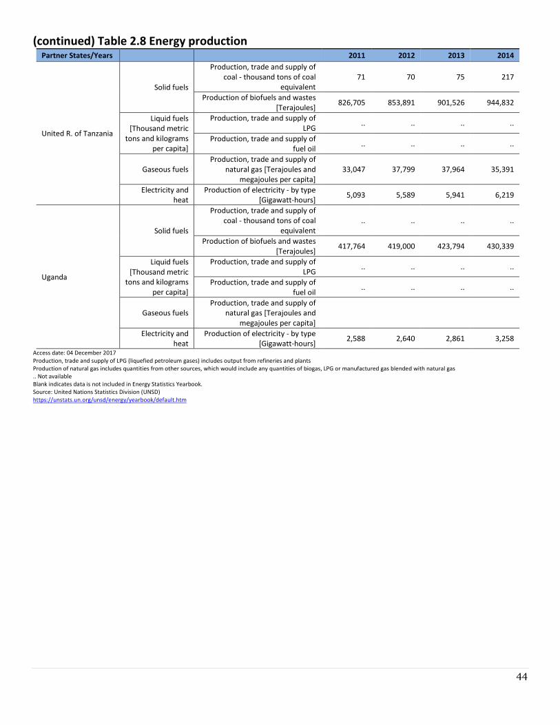
44
(continued) Table 2.8 Energy production Partner States/Years 2011 2012 2013 2014
United R. of Tanzania
Solid fuels
Production, trade and supply of
coal - thousand tons of coal
equivalent
71 70 75 217
Production of biofuels and wastes
[Terajoules] 826,705 853,891 901,526 944,832
Liquid fuels
[Thousand metric
tons and kilograms
per capita]
Production, trade and supply of
LPG .. .. .. ..
Production, trade and supply of
fuel oil .. .. .. ..
Gaseous fuels
Production, trade and supply of
natural gas [Terajoules and
megajoules per capita]
33,047 37,799 37,964 35,391
Electricity and
heat
Production of electricity - by type
[Gigawatt-hours] 5,093 5,589 5,941 6,219
Uganda
Solid fuels
Production, trade and supply of
coal - thousand tons of coal
equivalent
.. .. .. ..
Production of biofuels and wastes
[Terajoules] 417,764 419,000 423,794 430,339
Liquid fuels
[Thousand metric
tons and kilograms
per capita]
Production, trade and supply of
LPG .. .. .. ..
Production, trade and supply of
fuel oil .. .. .. ..
Gaseous fuels
Production, trade and supply of
natural gas [Terajoules and
megajoules per capita]
Electricity and
heat
Production of electricity - by type
[Gigawatt-hours] 2,588 2,640 2,861 3,258
Access date: 04 December 2017
Production, trade and supply of LPG (liquefied petroleum gases) includes output from refineries and plants
Production of natural gas includes quantities from other sources, which would include any quantities of biogas, LPG or manufactured gas blended with natural gas
.. Not available
Blank indicates data is not included in Energy Statistics Yearbook.
Source: United Nations Statistics Division (UNSD)
https://unstats.un.org/unsd/energy/yearbook/default.htm
45
Metadata for Table 2.8
Definitions
Production of energy is defined as the capture, extraction or manufacture of fuels or other energy products in forms which are
ready for general consumption. Energy production corresponds to the production of energy products.
• Solid fuels include hard and brown coal, peat, patent fuel, brown coal briquettes, peat products, coal coke, oil shale and
other products not specified.
• Solid biofuels include production of biofuels and wastes such as Fuelwood, Animal waste, Vegetal waste, Bagasse, Black
liquor and Charcoal.
• Liquid fuels include crude oil, natural gas liquid, additives and oxygenates, oil products, gasoline, kerosene, gas/diesel oil,
fuel oil, LPG, ethane, refinery gas, naphtha, spirits, lubricants, bitumen, paraffin waxes, petroleum coke and other oil
products not specified.
• Gaseous fuels include natural gas, gas works gas, coke oven gas, blast furnace gas and other recovered gases not specified.
• Electricity and heat refers to production of energy such as streaming water, wind or waves, conversion of solar radiation
to photovoltaic processes or combustion of fuels.
Relevance
There are many environmental issues related to energy production, including: (i) the depletion of non-renewable energy resources;
(ii) the destruction of the environment (landscape) by the extraction of energy resources and the production and distribution of
energy, and (iii) the pollution (air, water and soil) and waste generated by the production and consumption of energy. For statistical
purposes, energy is measured in its “usable form” embedded in energy products.
Computation/Collection Method
Data are being collected from the countries through a questionnaire and processed by UNSD.
Source
UNSD,
https://unstats.un.org/unsd/energy/yearbook/2014/t17.pdf
https://unstats.un.org/unsd/energy/yearbook/2014/t12.pdf
https://unstats.un.org/unsd/energy/yearbook/2014/t27.pdf
https://unstats.un.org/unsd/energy/yearbook/2014/04d.pdf
https://unstats.un.org/unsd/environment/FDES/MS%202.2%20Energy%20Resources.pdf
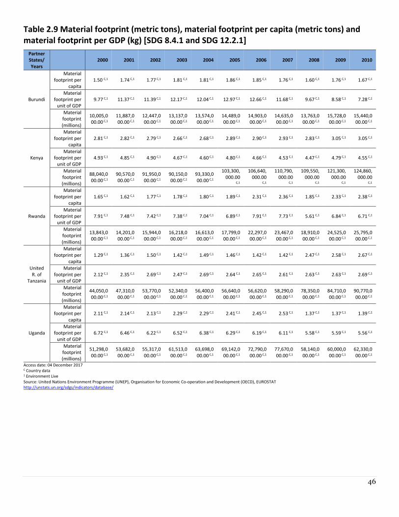
46
Table 2.9 Material footprint (metric tons), material footprint per capita (metric tons) and
material footprint per GDP (kg) [SDG 8.4.1 and SDG 12.2.1]
Partner
States/
Years
2000 2001 2002 2003 2004 2005 2006 2007 2008 2009 2010
Burundi
Material
footprint per
capita
1.50 C,1 1.74 C,1 1.77 C,1 1.81 C,1 1.81 C,1 1.86 C,1 1.85 C,1 1.76 C,1 1.60 C,1 1.76 C,1 1.67 C,1
Material
footprint per
unit of GDP
9.77 C,1 11.37 C,1 11.39 C,1 12.17 C,1 12.04 C,1 12.97 C,1 12.66 C,1 11.68 C,1 9.67 C,1 8.58 C,1 7.28 C,1
Material
footprint
(millions)
10,005,0
00.00 C,1
11,887,0
00.00 C,1
12,447,0
00.00 C,1
13,137,0
00.00 C,1
13,574,0
00.00 C,1
14,489,0
00.00 C,1
14,903,0
00.00 C,1
14,635,0
00.00 C,1
13,763,0
00.00 C,1
15,728,0
00.00 C,1
15,440,0
00.00 C,1
Kenya
Material
footprint per
capita
2.81 C,1 2.82 C,1 2.79 C,1 2.66 C,1 2.68 C,1 2.89 C,1 2.90 C,1 2.93 C,1 2.83 C,1 3.05 C,1 3.05 C,1
Material
footprint per
unit of GDP
4.93 C,1 4.85 C,1 4.90 C,1 4.67 C,1 4.60 C,1 4.80 C,1 4.66 C,1 4.53 C,1 4.47 C,1 4.79 C,1 4.55 C,1
Material
footprint
(millions)
88,040,0
00.00 C,1
90,570,0
00.00 C,1
91,950,0
00.00 C,1
90,150,0
00.00 C,1
93,330,0
00.00 C,1
103,300,
000.00
C,1
106,640,
000.00
C,1
110,790,
000.00
C,1
109,550,
000.00
C,1
121,300,
000.00
C,1
124,860,
000.00
C,1
Rwanda
Material
footprint per
capita
1.65 C,1 1.62 C,1 1.77 C,1 1.78 C,1 1.80 C,1 1.89 C,1 2.31 C,1 2.36 C,1 1.85 C,1 2.33 C,1 2.38 C,1
Material
footprint per
unit of GDP
7.91 C,1 7.48 C,1 7.42 C,1 7.38 C,1 7.04 C,1 6.89 C,1 7.91 C,1 7.73 C,1 5.61 C,1 6.84 C,1 6.71 C,1
Material
footprint
(millions)
13,843,0
00.00 C,1
14,201,0
00.00 C,1
15,944,0
00.00 C,1
16,218,0
00.00 C,1
16,613,0
00.00 C,1
17,799,0
00.00 C,1
22,297,0
00.00 C,1
23,467,0
00.00 C,1
18,910,0
00.00 C,1
24,525,0
00.00 C,1
25,795,0
00.00 C,1
United
R. of
Tanzania
Material
footprint per
capita
1.29 C,1 1.36 C,1 1.50 C,1 1.42 C,1 1.49 C,1 1.46 C,1 1.42 C,1 1.42 C,1 2.47 C,1 2.58 C,1 2.67 C,1
Material
footprint per
unit of GDP
2.12 C,1 2.35 C,1 2.69 C,1 2.47 C,1 2.69 C,1 2.64 C,1 2.65 C,1 2.61 C,1 2.63 C,1 2.63 C,1 2.69 C,1
Material
footprint
(millions)
44,050,0
00.00 C,1
47,310,0
00.00 C,1
53,770,0
00.00 C,1
52,340,0
00.00 C,1
56,400,0
00.00 C,1
56,640,0
00.00 C,1
56,620,0
00.00 C,1
58,290,0
00.00 C,1
78,350,0
00.00 C,1
84,710,0
00.00 C,1
90,770,0
00.00 C,1
Uganda
Material
footprint per
capita
2.11 C,1 2.14 C,1 2.13 C,1 2.29 C,1 2.29 C,1 2.41 C,1 2.45 C,1 2.53 C,1 1.37 C,1 1.37 C,1 1.39 C,1
Material
footprint per
unit of GDP
6.72 C,1 6.46 C,1 6.22 C,1 6.52 C,1 6.38 C,1 6.29 C,1 6.19 C,1 6.11 C,1 5.58 C,1 5.59 C,1 5.56 C,1
Material
footprint
(millions)
51,298,0
00.00 C,1
53,682,0
00.00 C,1
55,317,0
00.00 C,1
61,513,0
00.00 C,1
63,698,0
00.00 C,1
69,142,0
00.00 C,1
72,790,0
00.00 C,1
77,670,0
00.00 C,1
58,140,0
00.00 C,1
60,000,0
00.00 C,1
62,330,0
00.00 C,1
Access date: 04 December 2017 C Country data 1 Environment Live
Source: United Nations Environment Programme (UNEP), Organisation for Economic Co-operation and Development (OECD), EUROSTAT
http://unstats.un.org/sdgs/indicators/database/
47
Metadata for Table 2.9
Definition
Material footprint is the attribution of global material extraction to domestic final demand of a country. The total material footprint
is the sum of the material footprint for biomass, fossil fuels, metal ores and non-metal ores.
Relevance
Material footprint of consumption reports the amount of primary materials required to serve final demand of a country and can
be interpreted as an indicator for the material standard of living and/or level of capitalization of an economy. Per-capita material
footprint describes the average material use for final demand.
Computation/Collection Method
It is calculated as raw material equivalent of imports plus domestic extraction minus raw material equivalents of exports. For the
attribution of the primary material needs of final demand a global, multi-regional input-output framework is employed. The
attribution method based on I-O analytical tools is described in detail in Wiedmann et al. 2015.
Source
UNEP, https://unstats.un.org/sdgs/metadata/files/Metadata-08-04-01.pdf
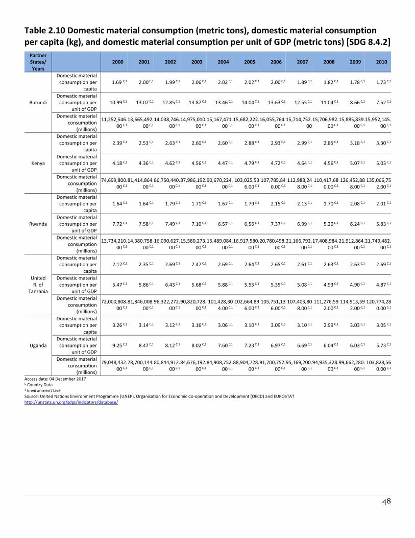
48
Table 2.10 Domestic material consumption (metric tons), domestic material consumption
per capita (kg), and domestic material consumption per unit of GDP (metric tons) [SDG 8.4.2]
Partner
States/
Years
2000 2001 2002 2003 2004 2005 2006 2007 2008 2009 2010
Burundi
Domestic material
consumption per
capita
1.69 C,1 2.00 C,1 1.99 C,1 2.06 C,1 2.02 C,1 2.02 C,1 2.00 C,1 1.89 C,1 1.82 C,1 1.78 C,1 1.73 C,1
Domestic material
consumption per
unit of GDP
10.99 C,1 13.07 C,1 12.85 C,1 13.87 C,1 13.46 C,1 14.04 C,1 13.63 C,1 12.55 C,1 11.04 C,1 8.66 C,1 7.52 C,1
Domestic material
consumption
(millions)
11,252,546.
00 C,1
13,665,492.
00 C,1
14,038,746.
00 C,1
14,975,010.
00 C,1
15,167,471.
00 C,1
15,682,222.
00 C,1
16,055,764.
00 C,1
15,714,752.
00
15,706,982.
00 C,1
15,885,839.
00 C,1
15,952,145.
00 C,1
Kenya
Domestic material
consumption per
capita
2.39 C,1 2.53 C,1 2.63 C,1 2.60 C,1 2.60 C,1 2.88 C,1 2.93 C,1 2.99 C,1 2.85 C,1 3.18 C,1 3.30 C,1
Domestic material
consumption per
unit of GDP
4.18 C,1 4.36 C,1 4.62 C,1 4.56 C,1 4.47 C,1 4.79 C,1 4.72 C,1 4.64 C,1 4.56 C,1 5.07 C,1 5.03 C,1
Domestic material
consumption
(millions)
74,699,800.
00 C,1
81,414,864.
00 C,1
86,750,440.
00 C,1
87,986,192.
00 C,1
90,670,224.
00 C,1
103,025,53
6.00 C,1
107,785,84
0.00 C,1
112,988,24
8.00 C,1
110,417,68
0.00 C,1
126,452,88
8.00 C,1
135,066,75
2.00 C,1
Rwanda
Domestic material
consumption per
capita
1.64 C,1 1.64 C,1 1.79 C,1 1.71 C,1 1.67 C,1 1.79 C,1 2.15 C,1 2.13 C,1 1.70 C,1 2.08 C,1 2.01 C,1
Domestic material
consumption per
unit of GDP
7.72 C,1 7.58 C,1 7.49 C,1 7.10 C,1 6.57 C,1 6.56 C,1 7.37 C,1 6.99 C,1 5.20 C,1 6.24 C,1 5.83 C,1
Domestic material
consumption
(millions)
13,734,210.
00 C,1
14,380,758.
00 C,1
16,090,627.
00 C,1
15,580,273.
00 C,1
15,489,084.
00 C,1
16,917,580.
00 C,1
20,780,498.
00 C,1
21,166,792.
00 C,1
17,408,984.
00 C,1
21,912,864.
00 C,1
21,749,482.
00 C,1
United
R. of
Tanzania
Domestic material
consumption per
capita
2.12 C,1 2.35 C,1 2.69 C,1 2.47 C,1 2.69 C,1 2.64 C,1 2.65 C,1 2.61 C,1 2.63 C,1 2.63 C,1 2.69 C,1
Domestic material
consumption per
unit of GDP
5.47 C,1 5.86 C,1 6.43 C,1 5.68 C,1 5.88 C,1 5.55 C,1 5.35 C,1 5.08 C,1 4.93 C,1 4.90 C,1 4.87 C,1
Domestic material
consumption
(millions)
72,000,808.
00 C,1
81,846,008.
00 C,1
96,322,272.
00 C,1
90,820,728.
00 C,1
101,428,30
4.00 C,1
102,664,89
6.00 C,1
105,751,13
6.00 C,1
107,403,80
8.00 C,1
111,276,59
2.00 C,1
114,913,59
2.00 C,1
120,774,28
0.00 C,1
Uganda
Domestic material
consumption per
capita
3.26 C,1 3.14 C,1 3.12 C,1 3.16 C,1 3.06 C,1 3.10 C,1 3.09 C,1 3.10 C,1 2.99 C,1 3.03 C,1 3.05 C,1
Domestic material
consumption per
unit of GDP
9.25 C,1 8.47 C,1 8.12 C,1 8.02 C,1 7.60 C,1 7.23 C,1 6.97 C,1 6.69 C,1 6.04 C,1 6.03 C,1 5.73 C,1
Domestic material
consumption
(millions)
79,048,432.
00 C,1
78,700,144.
00 C,1
80,844,912.
00 C,1
84,676,192.
00 C,1
84,908,752.
00 C,1
88,904,728.
00 C,1
91,700,752.
00 C,1
95,169,200.
00 C,1
94,935,328.
00 C,1
99,662,280.
00 C,1
103,828,56
0.00 C,1
Access date: 04 December 2017 C Country Data 1 Environment Live
Source: United Nations Environment Programme (UNEP), Organisation for Economic Co-operation and Development (OECD) and EUROSTAT
http://unstats.un.org/sdgs/indicators/database/
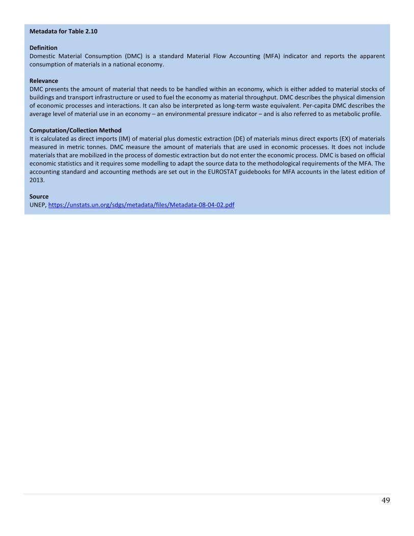
49
Metadata for Table 2.10
Definition
Domestic Material Consumption (DMC) is a standard Material Flow Accounting (MFA) indicator and reports the apparent
consumption of materials in a national economy.
Relevance
DMC presents the amount of material that needs to be handled within an economy, which is either added to material stocks of
buildings and transport infrastructure or used to fuel the economy as material throughput. DMC describes the physical dimension
of economic processes and interactions. It can also be interpreted as long-term waste equivalent. Per-capita DMC describes the
average level of material use in an economy – an environmental pressure indicator – and is also referred to as metabolic profile.
Computation/Collection Method
It is calculated as direct imports (IM) of material plus domestic extraction (DE) of materials minus direct exports (EX) of materials
measured in metric tonnes. DMC measure the amount of materials that are used in economic processes. It does not include
materials that are mobilized in the process of domestic extraction but do not enter the economic process. DMC is based on official
economic statistics and it requires some modelling to adapt the source data to the methodological requirements of the MFA. The
accounting standard and accounting methods are set out in the EUROSTAT guidebooks for MFA accounts in the latest edition of
2013.
Source
UNEP, https://unstats.un.org/sdgs/metadata/files/Metadata-08-04-02.pdf
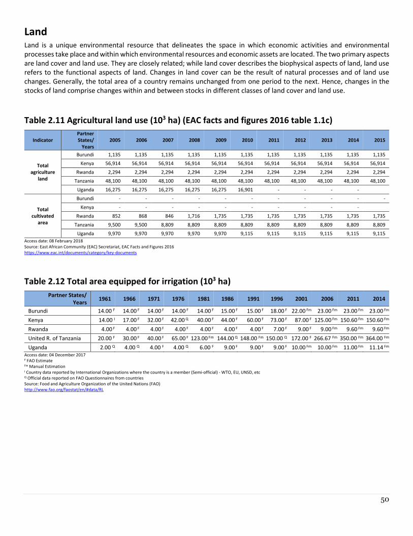
50
Land Land is a unique environmental resource that delineates the space in which economic activities and environmental
processes take place and within which environmental resources and economic assets are located. The two primary aspects
are land cover and land use. They are closely related; while land cover describes the biophysical aspects of land, land use
refers to the functional aspects of land. Changes in land cover can be the result of natural processes and of land use
changes. Generally, the total area of a country remains unchanged from one period to the next. Hence, changes in the
stocks of land comprise changes within and between stocks in different classes of land cover and land use.
Table 2.11 Agricultural land use (103 ha) (EAC facts and figures 2016 table 1.1c)
Indicator
Partner
States/
Years
2005 2006 2007 2008 2009 2010 2011 2012 2013 2014 2015
Total
agriculture
land
Burundi 1,135 1,135 1,135 1,135 1,135 1,135 1,135 1,135 1,135 1,135 1,135
Kenya 56,914 56,914 56,914 56,914 56,914 56,914 56,914 56,914 56,914 56,914 56,914
Rwanda 2,294 2,294 2,294 2,294 2,294 2,294 2,294 2,294 2,294 2,294 2,294
Tanzania 48,100 48,100 48,100 48,100 48,100 48,100 48,100 48,100 48,100 48,100 48,100
Uganda 16,275 16,275 16,275 16,275 16,275 16,901 - - - -
Total
cultivated
area
Burundi - - - - - - - - - - -
Kenya - - - - - - - - - -
Rwanda 852 868 846 1,716 1,735 1,735 1,735 1,735 1,735 1,735 1,735
Tanzania 9,500 9,500 8,809 8,809 8,809 8,809 8,809 8,809 8,809 8,809 8,809
Uganda 9,970 9,970 9,970 9,970 9,970 9,115 9,115 9,115 9,115 9,115 9,115
Access date: 08 February 2018
Source: East African Community (EAC) Secretariat, EAC Facts and Figures 2016
https://www.eac.int/documents/category/key-documents
Table 2.12 Total area equipped for irrigation (103 ha)
Partner States/
Years 1961 1966 1971 1976 1981 1986 1991 1996 2001 2006 2011 2014
Burundi 14.00 F 14.00 F 14.00 F 14.00 F 14.00 F 15.00 F 15.00 F 18.00 F 22.00 Fm 23.00 Fm 23.00 Fm 23.00 Fm
Kenya 14.00 I 17.00 F 32.00 F 42.00 Q 40.00 F 44.00 F 60.00 F 73.00 F 87.00 F 125.00 Fm 150.60 Fm 150.60 Fm
Rwanda 4.00 F 4.00 F 4.00 F 4.00 F 4.00 F 4.00 F 4.00 F 7.00 F 9.00 F 9.00 Fm 9.60 Fm 9.60 Fm
United R. of Tanzania 20.00 F 30.00 F 40.00 F 65.00 F 123.00 Fm 144.00 Q 148.00 Fm 150.00 Q 172.00 F 266.67 Fm 350.00 Fm 364.00 Fm
Uganda 2.00 Q 4.00 Q 4.00 F 4.00 Q 6.00 F 9.00 F 9.00 F 9.00 F 10.00 Fm 10.00 Fm 11.00 Fm 11.14 Fm
Access date: 04 December 2017 F FAO Estimate Fm Manual Estimation
I Country data reported by International Organizations where the country is a member (Semi-official) - WTO, EU, UNSD, etc Q Official data reported on FAO Questionnaires from countries
Source: Food and Agriculture Organization of the United Nations (FAO)
http://www.fao.org/faostat/en/#data/RL
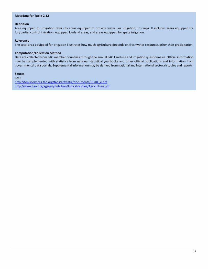
51
Metadata for Table 2.12
Definition
Area equipped for irrigation refers to areas equipped to provide water (via irrigation) to crops. It includes areas equipped for
full/partial control irrigation, equipped lowland areas, and areas equipped for spate irrigation.
Relevance
The total area equipped for irrigation illustrates how much agriculture depends on freshwater resources other than precipitation.
Computation/Collection Method
Data are collected from FAO member Countries through the annual FAO Land use and irrigation questionnaire. Official information
may be complemented with statistics from national statistical yearbooks and other official publications and information from
governmental data portals. Supplemental information may be derived from national and international sectoral studies and reports.
Source
FAO,
http://fenixservices.fao.org/faostat/static/documents/RL/RL_e.pdf
http://www.fao.org/ag/agn/nutrition/Indicatorsfiles/Agriculture.pdf
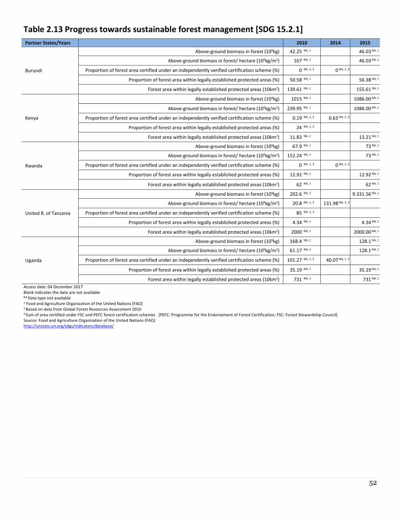
52
Table 2.13 Progress towards sustainable forest management [SDG 15.2.1]
Partner States/Years 2010 2014 2015
Burundi
Above-ground biomass in forest (109kg) 42.25 NA, 1 46.03 NA, 1
Above-ground biomass in forest/ hectare (105kg/m2) 167 NA, 1 46.03 NA, 1
Proportion of forest area certified under an independently verified certification scheme (%) 0 NA, 1, 3 0 NA, 1, 3
Proportion of forest area within legally established protected areas (%) 50.58 NA, 1 56.38 NA, 1
Forest area within legally established protected areas (10km2) 139.61 NA, 1 155.61 NA, 1
Kenya
Above-ground biomass in forest (109kg) 1015 NA, 1 1086.00 NA, 1
Above-ground biomass in forest/ hectare (105kg/m2) 239.95 NA, 1 1086.00 NA, 1
Proportion of forest area certified under an independently verified certification scheme (%) 0.19 NA, 1, 3 0.63 NA, 1, 3
Proportion of forest area within legally established protected areas (%) 24 NA, 1, 2
Forest area within legally established protected areas (10km2) 11.83 NA, 1 13.21 NA, 1
Rwanda
Above-ground biomass in forest (109kg) 67.9 NA, 1 73 NA, 1
Above-ground biomass in forest/ hectare (105kg/m2) 152.24 NA, 1 73 NA, 1
Proportion of forest area certified under an independently verified certification scheme (%) 0 NA, 1, 3 0 NA, 1, 3
Proportion of forest area within legally established protected areas (%) 12.92 NA, 1 12.92 NA, 1
Forest area within legally established protected areas (10km2) 62 NA, 1 62 NA, 1
United R. of Tanzania
Above-ground biomass in forest (109kg) 202.6 NA, 1 9.331.56 NA, 1
Above-ground biomass in forest/ hectare (105kg/m2) 20.8 NA, 1, 3 131.98 NA, 1, 3
Proportion of forest area certified under an independently verified certification scheme (%) 85 NA, 1, 2
Proportion of forest area within legally established protected areas (%) 4.34 NA, 1 4.34 NA, 1
Forest area within legally established protected areas (10km2) 2000 NA, 1 2000.00 NA, 1
Uganda
Above-ground biomass in forest (109kg) 168.4 NA, 1 128.1 NA, 1
Above-ground biomass in forest/ hectare (105kg/m2) 61.17 NA, 1 128.1 NA, 1
Proportion of forest area certified under an independently verified certification scheme (%) 101.27 NA, 1, 3 40.07 NA, 1, 3
Proportion of forest area within legally established protected areas (%) 35.19 NA, 1 35.19 NA, 1
Forest area within legally established protected areas (10km2) 731 NA, 1 731 NA, 1
Access date: 04 December 2017
Blank indicates the data are not available NA Data type not available 1 Food and Agriculture Organization of the United Nations (FAO) 2 Based on data from Global Forest Resources Assessment 2010 3 Sum of area certified under FSC and PEFC forest certification schemes [PEFC: Programme for the Endorsement of Forest Certification; FSC: Forest Stewardship Council]
Source: Food and Agriculture Organization of the United Nations (FAO)
http://unstats.un.org/sdgs/indicators/database/
53
Metadata for Table 2.13
Definition
Sustainable forest management is a dynamic and evolving concept that aims to maintain and enhance the economic, social and
environmental values of all types of forests, for the benefit of present and future generations
Relevance
The definition of sustainable forest management (SFM) by the UN General Assembly contains several key aspects, notably that
sustainable forest management is a concept which varies over time and between countries, whose circumstances – ecological,
social and economic – vary widely, but that it should always address a wide range of forest values, including economic, social and
environmental values, and take intergenerational equity into account.
Clearly a simple measure of forest area, while essential, and used for target 15.1, is insufficient to monitor sustainable forest
management as a whole. Five sub-indicators are developed to measure this topic.
Computation/Collection Method
At national level, forest area, biomass stock, forest area within protected areas, forest area under management plan and forest
area under an independently verified forest management certification scheme are reported directly to FAO for pre-established
reference years. Based on the country reported data, FAO then makes country-level estimates of the forest area net change rate
using the compound interest formula, and also the proportion of forest area within protected area and under management plan.
Source
GA, UN, http://www.un.org/en/ga/search/view_doc.asp?symbol=A/RES/62/98 FAO, https://unstats.un.org/sdgs/metadata/files/Metadata-15-02-01.pdf
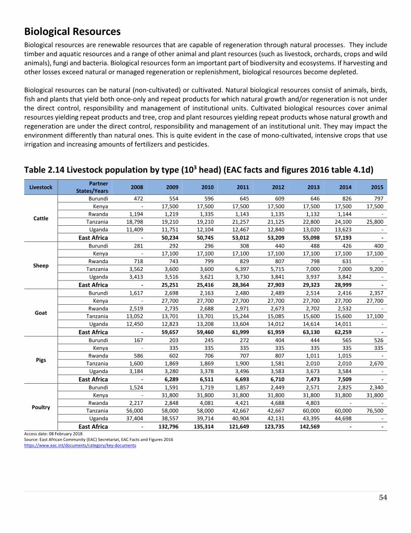
54
Biological Resources Biological resources are renewable resources that are capable of regeneration through natural processes. They include
timber and aquatic resources and a range of other animal and plant resources (such as livestock, orchards, crops and wild
animals), fungi and bacteria. Biological resources form an important part of biodiversity and ecosystems. If harvesting and
other losses exceed natural or managed regeneration or replenishment, biological resources become depleted.
Biological resources can be natural (non-cultivated) or cultivated. Natural biological resources consist of animals, birds,
fish and plants that yield both once-only and repeat products for which natural growth and/or regeneration is not under
the direct control, responsibility and management of institutional units. Cultivated biological resources cover animal
resources yielding repeat products and tree, crop and plant resources yielding repeat products whose natural growth and
regeneration are under the direct control, responsibility and management of an institutional unit. They may impact the
environment differently than natural ones. This is quite evident in the case of mono-cultivated, intensive crops that use
irrigation and increasing amounts of fertilizers and pesticides.
Table 2.14 Livestock population by type (103 head) (EAC facts and figures 2016 table 4.1d)
Livestock Partner
States/Years 2008 2009 2010 2011 2012 2013 2014 2015
Cattle
Burundi 472 554 596 645 609 646 826 797
Kenya - 17,500 17,500 17,500 17,500 17,500 17,500 17,500
Rwanda 1,194 1,219 1,335 1,143 1,135 1,132 1,144 -
Tanzania 18,798 19,210 19,210 21,257 21,125 22,800 24,100 25,800
Uganda 11,409 11,751 12,104 12,467 12,840 13,020 13,623 -
East Africa - 50,234 50,745 53,012 53,209 55,098 57,193 -
Sheep
Burundi 281 292 296 308 440 488 426 400
Kenya - 17,100 17,100 17,100 17,100 17,100 17,100 17,100
Rwanda 718 743 799 829 807 798 631 -
Tanzania 3,562 3,600 3,600 6,397 5,715 7,000 7,000 9,200
Uganda 3,413 3,516 3,621 3,730 3,841 3,937 3,842 -
East Africa - 25,251 25,416 28,364 27,903 29,323 28,999 -
Goat
Burundi 1,617 2,698 2,163 2,480 2,489 2,514 2,416 2,357
Kenya - 27,700 27,700 27,700 27,700 27,700 27,700 27,700
Rwanda 2,519 2,735 2,688 2,971 2,673 2,702 2,532 -
Tanzania 13,052 13,701 13,701 15,244 15,085 15,600 15,600 17,100
Uganda 12,450 12,823 13,208 13,604 14,012 14,614 14,011 -
East Africa - 59,657 59,460 61,999 61,959 63,130 62,259 -
Pigs
Burundi 167 203 245 272 404 444 565 526
Kenya - 335 335 335 335 335 335 335
Rwanda 586 602 706 707 807 1,011 1,015 -
Tanzania 1,600 1,869 1,869 1,900 1,581 2,010 2,010 2,670
Uganda 3,184 3,280 3,378 3,496 3,583 3,673 3,584 -
East Africa - 6,289 6,511 6,693 6,710 7,473 7,509 -
Poultry
Burundi 1,524 1,591 1,719 1,857 2,449 2,571 2,825 2,340
Kenya - 31,800 31,800 31,800 31,800 31,800 31,800 31,800
Rwanda 2,217 2,848 4,081 4,421 4,688 4,803 - -
Tanzania 56,000 58,000 58,000 42,667 42,667 60,000 60,000 76,500
Uganda 37,404 38,557 39,714 40,904 42,131 43,395 44,698 -
East Africa - 132,796 135,314 121,649 123,735 142,569 - - Access date: 08 February 2018
Source: East African Community (EAC) Secretariat, EAC Facts and Figures 2016
https://www.eac.int/documents/category/key-documents
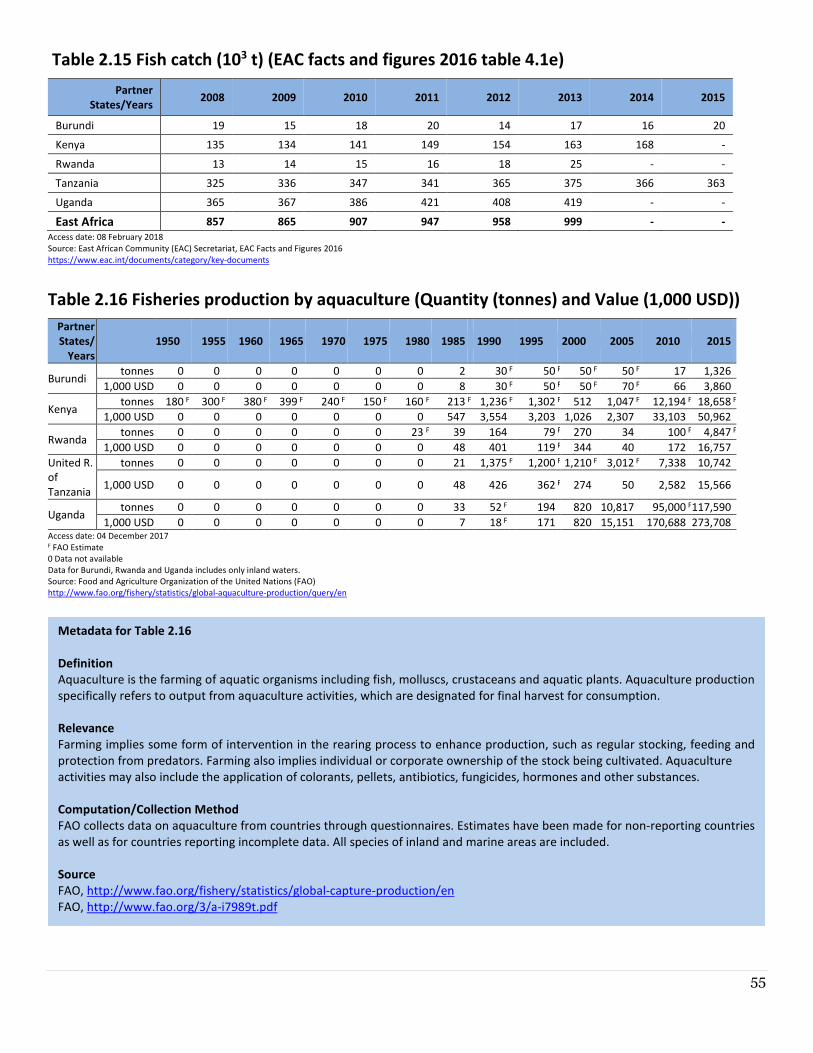
55
Table 2.15 Fish catch (103 t) (EAC facts and figures 2016 table 4.1e)
Partner
States/Years 2008 2009 2010 2011 2012 2013 2014 2015
Burundi 19 15 18 20 14 17 16 20
Kenya 135 134 141 149 154 163 168 -
Rwanda 13 14 15 16 18 25 - -
Tanzania 325 336 347 341 365 375 366 363
Uganda 365 367 386 421 408 419 - -
East Africa 857 865 907 947 958 999 - -
Access date: 08 February 2018
Source: East African Community (EAC) Secretariat, EAC Facts and Figures 2016
https://www.eac.int/documents/category/key-documents
Table 2.16 Fisheries production by aquaculture (Quantity (tonnes) and Value (1,000 USD))
Partner
States/
Years
1950 1955 1960 1965 1970 1975 1980 1985 1990 1995 2000 2005 2010 2015
Burundi tonnes 0 0 0 0 0 0 0 2 30 F 50 F 50 F 50 F 17 1,326
1,000 USD 0 0 0 0 0 0 0 8 30 F 50 F 50 F 70 F 66 3,860
Kenya tonnes 180 F 300 F 380 F 399 F 240 F 150 F 160 F 213 F 1,236 F 1,302 F 512 1,047 F 12,194 F 18,658 F
1,000 USD 0 0 0 0 0 0 0 547 3,554 3,203 1,026 2,307 33,103 50,962
Rwanda tonnes 0 0 0 0 0 0 23 F 39 164 79 F 270 34 100 F 4,847 F
1,000 USD 0 0 0 0 0 0 0 48 401 119 F 344 40 172 16,757
United R.
of
Tanzania
tonnes 0 0 0 0 0 0 0 21 1,375 F 1,200 F 1,210 F 3,012 F 7,338 10,742
1,000 USD 0 0 0 0 0 0 0 48 426 362 F 274 50 2,582 15,566
Uganda tonnes 0 0 0 0 0 0 0 33 52 F 194 820 10,817 95,000 F117,590
1,000 USD 0 0 0 0 0 0 0 7 18 F 171 820 15,151 170,688 273,708 Access date: 04 December 2017 F FAO Estimate
0 Data not available
Data for Burundi, Rwanda and Uganda includes only inland waters.
Source: Food and Agriculture Organization of the United Nations (FAO)
http://www.fao.org/fishery/statistics/global-aquaculture-production/query/en
Metadata for Table 2.16
Definition
Aquaculture is the farming of aquatic organisms including fish, molluscs, crustaceans and aquatic plants. Aquaculture production
specifically refers to output from aquaculture activities, which are designated for final harvest for consumption.
Relevance
Farming implies some form of intervention in the rearing process to enhance production, such as regular stocking, feeding and
protection from predators. Farming also implies individual or corporate ownership of the stock being cultivated. Aquaculture
activities may also include the application of colorants, pellets, antibiotics, fungicides, hormones and other substances.
Computation/Collection Method
FAO collects data on aquaculture from countries through questionnaires. Estimates have been made for non-reporting countries
as well as for countries reporting incomplete data. All species of inland and marine areas are included.
Source
FAO, http://www.fao.org/fishery/statistics/global-capture-production/en
FAO, http://www.fao.org/3/a-i7989t.pdf
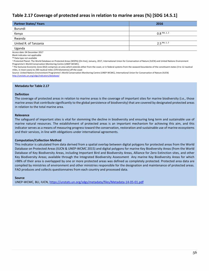
56
Table 2.17 Coverage of protected areas in relation to marine areas (%) [SDG 14.5.1]
Partner States/ Years 2016
Burundi
Kenya 0.8 NA, 1, 2
Rwanda
United R. of Tanzania 2.5 NA, 1, 2
Uganda Access date: 04 December 2017
Blank indicates not applicable NA Data type not available 1 Protected Planet: The World Database on Protected Areas (WDPA) [On-line], January, 2017, International Union for Conservation of Nature (IUCN) and United Nations Environment
Programme's World Conservation Monitoring Centre (UNEP-WCMC). 2 The Exclusive Economic Zone (EEZ) comprises an area which extends either from the coast, or in federal systems from the seaward boundaries of the constituent states (3 to 12 nautical
miles, in most cases) to 200 nautical miles (370 kilometres) off the coast
Source: United Nations Environment Programme’s World Conservation Monitoring Centre (UNEP-WCMC), International Union for Conservation of Nature (IUCN)
http://unstats.un.org/sdgs/indicators/database/
Metadata for Table 2.17
Definition
The coverage of protected areas in relation to marine areas is the coverage of important sites for marine biodiversity (i.e., those
marine areas that contribute significantly to the global persistence of biodiversity) that are covered by designated protected areas
in relation to the total marine area.
Relevance
The safeguard of important sites is vital for stemming the decline in biodiversity and ensuring long term and sustainable use of
marine natural resources. The establishment of protected areas is an important mechanism for achieving this aim, and this
indicator serves as a means of measuring progress toward the conservation, restoration and sustainable use of marine ecosystems
and their services, in line with obligations under international agreements.
Computation/Collection Method
This indicator is calculated from data derived from a spatial overlap between digital polygons for protected areas from the World
Database on Protected Areas (IUCN & UNEP-WCMC 2015) and digital polygons for marine Key Biodiversity Areas (from the World
Database of Key Biodiversity Areas, including Important Bird and Biodiversity Areas, Alliance for Zero Extinction sites, and other
Key Biodiversity Areas; available through the Integrated Biodiversity Assessment Any marine Key Biodiversity Areas for which
>98% of their area is overlapped by one or more protected areas was defined as completely protected. Protected area data are
compiled by ministries of environment and other ministries responsible for the designation and maintenance of protected areas.
FAO produces and collects questionnaires from each country and processed data.
Source
UNEP-WCMC, BLI, IUCN, https://unstats.un.org/sdgs/metadata/files/Metadata-14-05-01.pdf
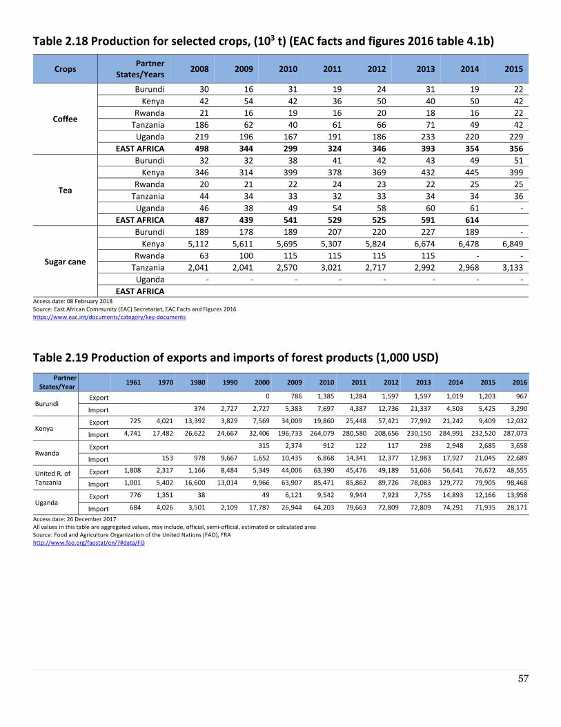
57
Table 2.18 Production for selected crops, (103 t) (EAC facts and figures 2016 table 4.1b)
Crops Partner
States/Years 2008 2009 2010 2011 2012 2013 2014 2015
Coffee
Burundi 30 16 31 19 24 31 19 22
Kenya 42 54 42 36 50 40 50 42
Rwanda 21 16 19 16 20 18 16 22
Tanzania 186 62 40 61 66 71 49 42
Uganda 219 196 167 191 186 233 220 229
EAST AFRICA 498 344 299 324 346 393 354 356
Tea
Burundi 32 32 38 41 42 43 49 51
Kenya 346 314 399 378 369 432 445 399
Rwanda 20 21 22 24 23 22 25 25
Tanzania 44 34 33 32 33 34 34 36
Uganda 46 38 49 54 58 60 61 -
EAST AFRICA 487 439 541 529 525 591 614
Sugar cane
Burundi 189 178 189 207 220 227 189 -
Kenya 5,112 5,611 5,695 5,307 5,824 6,674 6,478 6,849
Rwanda 63 100 115 115 115 115 - -
Tanzania 2,041 2,041 2,570 3,021 2,717 2,992 2,968 3,133
Uganda - - - - - - - -
EAST AFRICA Access date: 08 February 2018
Source: East African Community (EAC) Secretariat, EAC Facts and Figures 2016
https://www.eac.int/documents/category/key-documents
Table 2.19 Production of exports and imports of forest products (1,000 USD)
Partner
States/Year 1961 1970 1980 1990 2000 2009 2010 2011 2012 2013 2014 2015 2016
Burundi Export
0 786 1,385 1,284 1,597 1,597 1,019 1,203 967
Import
374 2,727 2,727 5,383 7,697 4,387 12,736 21,337 4,503 5,425 3,290
Kenya Export 725 4,021 13,392 3,829 7,569 34,009 19,860 25,448 57,421 77,992 21,242 9,409 12,032
Import 4,741 17,482 26,622 24,667 32,406 196,733 264,079 280,580 208,656 230,150 284,991 232,520 287,073
Rwanda Export
315 2,374 912 122 117 298 2,948 2,685 3,658
Import
153 978 9,667 1,652 10,435 6,868 14,341 12,377 12,983 17,927 21,045 22,689
United R. of
Tanzania
Export 1,808 2,317 1,166 8,484 5,349 44,006 63,390 45,476 49,189 51,606 56,641 76,672 48,555
Import 1,001 5,402 16,600 13,014 9,966 63,907 85,471 85,862 89,726 78,083 129,772 79,905 98,468
Uganda Export 776 1,351 38 49 6,121 9,542 9,944 7,923 7,755 14,893 12,166 13,958
Import 684 4,026 3,501 2,109 17,787 26,944 64,203 79,663 72,809 72,809 74,291 71,935 28,171
Access date: 26 December 2017
All values in this table are aggregated values, may include, official, semi-official, estimated or calculated area Source: Food and Agriculture Organization of the United Nations (FAO), FRA http://www.fao.org/faostat/en/?#data/FO
58
Metadata for Table 2.19
Definition
Total exports and imports of forest products (coniferous, non-coniferous tropical, non-coniferous non-tropical), including:
roundwood (wood fuel, including wood for charcoal, and industrial roundwood); wood charcoal, wood chips, particles and
residues; wood pellets and other agglomerates; sawnwood; wood-based panels (veneer sheets, plywood, particle board, oriented
strandboard (OSB) and similar board, and fireboard); wood pulp (mechanical wood pulp, semi-chemical wood pulp, chemical wood
pulp, dissolving grades), other pulp (pulp from fibres other than wood and recovered fibre pulp); recovered paper; and paper and
paperboard (graphic papers, sanitary and household papers, packaging materials, and other paper and paperboard not elsewhere
specified).
Relevance
Forest resources do not only play an important environmental role, but also an economic one through the production and trade
of forest products. The exports and imports of forest products in value shows the importance of forest resources in the trade
balance of a country.
Computation/Collection Method
FAO produces and collects questionnaires from each country. Some estimates have been made for non-reporting countries as well
as for countries reporting incomplete data.
Source
FAO, http://www.fao.org/forestry/34572-0902b3c041384fd87f2451da2bb9237.pdf
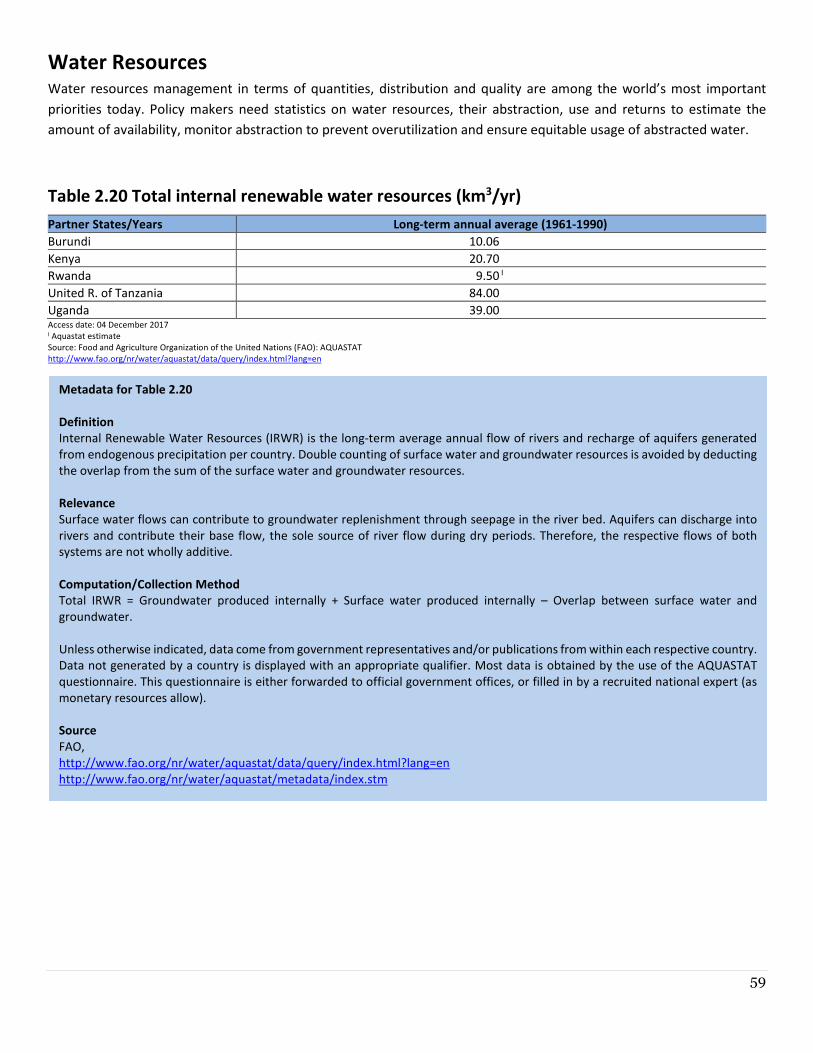
59
Water Resources Water resources management in terms of quantities, distribution and quality are among the world’s most important
priorities today. Policy makers need statistics on water resources, their abstraction, use and returns to estimate the
amount of availability, monitor abstraction to prevent overutilization and ensure equitable usage of abstracted water.
Table 2.20 Total internal renewable water resources (km3/yr)
Partner States/Years Long-term annual average (1961-1990)
Burundi 10.06
Kenya 20.70
Rwanda 9.50 I
United R. of Tanzania 84.00
Uganda 39.00 Access date: 04 December 2017 I Aquastat estimate
Source: Food and Agriculture Organization of the United Nations (FAO): AQUASTAT
http://www.fao.org/nr/water/aquastat/data/query/index.html?lang=en
Metadata for Table 2.20
Definition
Internal Renewable Water Resources (IRWR) is the long-term average annual flow of rivers and recharge of aquifers generated
from endogenous precipitation per country. Double counting of surface water and groundwater resources is avoided by deducting
the overlap from the sum of the surface water and groundwater resources.
Relevance
Surface water flows can contribute to groundwater replenishment through seepage in the river bed. Aquifers can discharge into
rivers and contribute their base flow, the sole source of river flow during dry periods. Therefore, the respective flows of both
systems are not wholly additive.
Computation/Collection Method
Total IRWR = Groundwater produced internally + Surface water produced internally – Overlap between surface water and
groundwater.
Unless otherwise indicated, data come from government representatives and/or publications from within each respective country.
Data not generated by a country is displayed with an appropriate qualifier. Most data is obtained by the use of the AQUASTAT
questionnaire. This questionnaire is either forwarded to official government offices, or filled in by a recruited national expert (as
monetary resources allow).
Source
FAO,
http://www.fao.org/nr/water/aquastat/data/query/index.html?lang=en
http://www.fao.org/nr/water/aquastat/metadata/index.stm
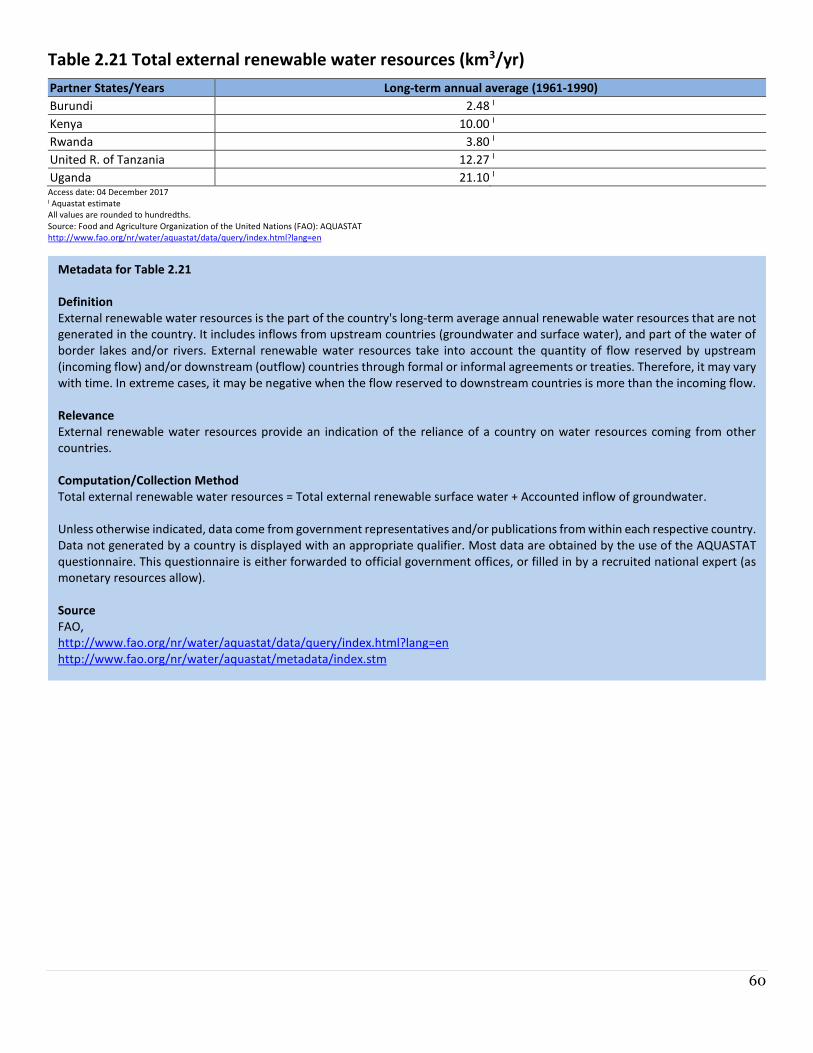
60
Table 2.21 Total external renewable water resources (km3/yr)
Partner States/Years Long-term annual average (1961-1990)
Burundi 2.48 I
Kenya 10.00 I
Rwanda 3.80 I
United R. of Tanzania 12.27 I
Uganda 21.10 I Access date: 04 December 2017 I Aquastat estimate
All values are rounded to hundredths.
Source: Food and Agriculture Organization of the United Nations (FAO): AQUASTAT
http://www.fao.org/nr/water/aquastat/data/query/index.html?lang=en
Metadata for Table 2.21
Definition
External renewable water resources is the part of the country's long-term average annual renewable water resources that are not
generated in the country. It includes inflows from upstream countries (groundwater and surface water), and part of the water of
border lakes and/or rivers. External renewable water resources take into account the quantity of flow reserved by upstream
(incoming flow) and/or downstream (outflow) countries through formal or informal agreements or treaties. Therefore, it may vary
with time. In extreme cases, it may be negative when the flow reserved to downstream countries is more than the incoming flow.
Relevance
External renewable water resources provide an indication of the reliance of a country on water resources coming from other
countries.
Computation/Collection Method
Total external renewable water resources = Total external renewable surface water + Accounted inflow of groundwater.
Unless otherwise indicated, data come from government representatives and/or publications from within each respective country.
Data not generated by a country is displayed with an appropriate qualifier. Most data are obtained by the use of the AQUASTAT
questionnaire. This questionnaire is either forwarded to official government offices, or filled in by a recruited national expert (as
monetary resources allow).
Source
FAO,
http://www.fao.org/nr/water/aquastat/data/query/index.html?lang=en
http://www.fao.org/nr/water/aquastat/metadata/index.stm
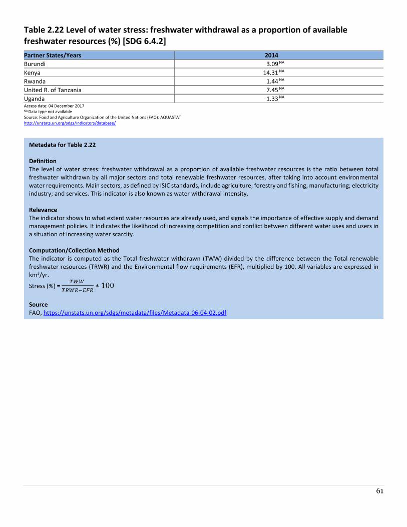
61
Table 2.22 Level of water stress: freshwater withdrawal as a proportion of available
freshwater resources (%) [SDG 6.4.2]
Partner States/Years 2014
Burundi 3.09 NA
Kenya 14.31 NA
Rwanda 1.44 NA
United R. of Tanzania 7.45 NA
Uganda 1.33 NA Access date: 04 December 2017 NA Data type not available
Source: Food and Agriculture Organization of the United Nations (FAO): AQUASTAT
http://unstats.un.org/sdgs/indicators/database/
Metadata for Table 2.22
Definition
The level of water stress: freshwater withdrawal as a proportion of available freshwater resources is the ratio between total
freshwater withdrawn by all major sectors and total renewable freshwater resources, after taking into account environmental
water requirements. Main sectors, as defined by ISIC standards, include agriculture; forestry and fishing; manufacturing; electricity
industry; and services. This indicator is also known as water withdrawal intensity.
Relevance
The indicator shows to what extent water resources are already used, and signals the importance of effective supply and demand
management policies. It indicates the likelihood of increasing competition and conflict between different water uses and users in
a situation of increasing water scarcity.
Computation/Collection Method
The indicator is computed as the Total freshwater withdrawn (TWW) divided by the difference between the Total renewable
freshwater resources (TRWR) and the Environmental flow requirements (EFR), multiplied by 100. All variables are expressed in
km3/yr.
Stress (%) = ���
��������∗ 100
Source
FAO, https://unstats.un.org/sdgs/metadata/files/Metadata-06-04-02.pdf
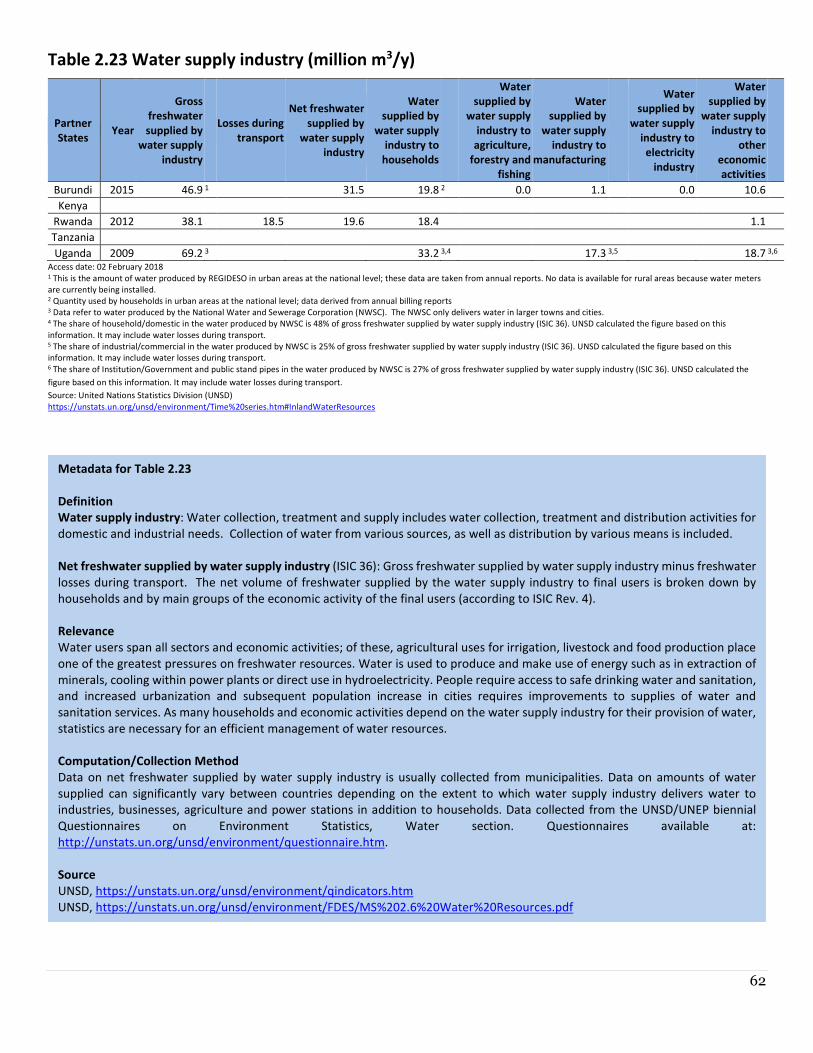
62
Table 2.23 Water supply industry (million m3/y)
Partner
States Year
Gross
freshwater
supplied by
water supply
industry
Losses during
transport
Net freshwater
supplied by
water supply
industry
Water
supplied by
water supply
industry to
households
Water
supplied by
water supply
industry to
agriculture,
forestry and
fishing
Water
supplied by
water supply
industry to
manufacturing
Water
supplied by
water supply
industry to
electricity
industry
Water
supplied by
water supply
industry to
other
economic
activities
Burundi 2015 46.9 1 31.5 19.8 2 0.0 1.1 0.0 10.6
Kenya
Rwanda 2012 38.1 18.5 19.6 18.4 1.1
Tanzania
Uganda 2009 69.2 3 33.2 3,4 17.3 3,5 18.7 3,6 Access date: 02 February 2018 1 This is the amount of water produced by REGIDESO in urban areas at the national level; these data are taken from annual reports. No data is available for rural areas because water meters
are currently being installed. 2 Quantity used by households in urban areas at the national level; data derived from annual billing reports 3 Data refer to water produced by the National Water and Sewerage Corporation (NWSC). The NWSC only delivers water in larger towns and cities. 4 The share of household/domestic in the water produced by NWSC is 48% of gross freshwater supplied by water supply industry (ISIC 36). UNSD calculated the figure based on this
information. It may include water losses during transport. 5 The share of industrial/commercial in the water produced by NWSC is 25% of gross freshwater supplied by water supply industry (ISIC 36). UNSD calculated the figure based on this
information. It may include water losses during transport. 6 The share of Institution/Government and public stand pipes in the water produced by NWSC is 27% of gross freshwater supplied by water supply industry (ISIC 36). UNSD calculated the
figure based on this information. It may include water losses during transport. Source: United Nations Statistics Division (UNSD)
https://unstats.un.org/unsd/environment/Time%20series.htm#InlandWaterResources
Metadata for Table 2.23
Definition
Water supply industry: Water collection, treatment and supply includes water collection, treatment and distribution activities for
domestic and industrial needs. Collection of water from various sources, as well as distribution by various means is included.
Net freshwater supplied by water supply industry (ISIC 36): Gross freshwater supplied by water supply industry minus freshwater
losses during transport. The net volume of freshwater supplied by the water supply industry to final users is broken down by
households and by main groups of the economic activity of the final users (according to ISIC Rev. 4).
Relevance
Water users span all sectors and economic activities; of these, agricultural uses for irrigation, livestock and food production place
one of the greatest pressures on freshwater resources. Water is used to produce and make use of energy such as in extraction of
minerals, cooling within power plants or direct use in hydroelectricity. People require access to safe drinking water and sanitation,
and increased urbanization and subsequent population increase in cities requires improvements to supplies of water and
sanitation services. As many households and economic activities depend on the water supply industry for their provision of water,
statistics are necessary for an efficient management of water resources.
Computation/Collection Method
Data on net freshwater supplied by water supply industry is usually collected from municipalities. Data on amounts of water
supplied can significantly vary between countries depending on the extent to which water supply industry delivers water to
industries, businesses, agriculture and power stations in addition to households. Data collected from the UNSD/UNEP biennial
Questionnaires on Environment Statistics, Water section. Questionnaires available at:
http://unstats.un.org/unsd/environment/questionnaire.htm.
Source
UNSD, https://unstats.un.org/unsd/environment/qindicators.htm
UNSD, https://unstats.un.org/unsd/environment/FDES/MS%202.6%20Water%20Resources.pdf
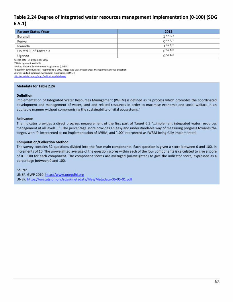
63
Table 2.24 Degree of integrated water resources management implementation (0-100) (SDG
6.5.1)
Partner States /Year 2012
Burundi 1 NA, 1, 2
Kenya 0 NA, 1, 2
Rwanda 1 NA, 1, 2
United R. of Tanzania 0 NA, 1, 2
Uganda 0 NA, 1, 2 Access date: 04 December 2017 NA Data type not available 1 United Nations Environment Programme (UNEP) 2 Based on 130 countries' response to a 2012 Integrated Water Resources Management survey question Source: United Nations Environment Programme (UNEP) http://unstats.un.org/sdgs/indicators/database/
Metadata for Table 2.24
Definition
Implementation of Integrated Water Resources Management (IWRM) is defined as “a process which promotes the coordinated
development and management of water, land and related resources in order to maximise economic and social welfare in an
equitable manner without compromising the sustainability of vital ecosystems.”
Relevance
The indicator provides a direct progress measurement of the first part of Target 6.5 “…implement integrated water resources
management at all levels …”. The percentage score provides an easy and understandable way of measuring progress towards the
target, with ‘0’ interpreted as no implementation of IWRM, and ‘100’ interpreted as IWRM being fully implemented.
Computation/Collection Method
The survey contains 32 questions divided into the four main components. Each question is given a score between 0 and 100, in
increments of 10. The un-weighted average of the question scores within each of the four components is calculated to give a score
of 0 – 100 for each component. The component scores are averaged (un-weighted) to give the indicator score, expressed as a
percentage between 0 and 100.
Source
UNEP, GWP 2010, http://www.unepdhi.org
UNEP, https://unstats.un.org/sdgs/metadata/files/Metadata-06-05-01.pdf
64
Chapter 3
Residuals

65
CHAPTER 3 RESIDUALS
This chapter contains statistics on the amount and characteristics of residuals generated by human production and
consumption processes, their management, and their final release to the environment. Residuals are flows of solid, liquid
and gaseous materials, and energy, that are discarded, discharged or emitted by establishments and households through
processes of production, consumption or accumulation. Residuals may be discarded, discharged or emitted directly to the
environment or be captured, collected, treated, recycled or reused. The FDES 2013 covers the main groups of residuals
that are emissions of substances to air, water or soil, wastewater and waste, and the release of residuals from the
application of chemical substances. This chapter does not contain indicators on wastewater.
Emissions to Air Emissions to air are gaseous and particulate substances released to the atmosphere by establishments and households as
a result of production, consumption and accumulation processes. The statistical description of such emissions covers their
sources and the quantities emitted by substance. These statistics can be used for evidence-based policy making,
particularly with regard to environmental regulations (e.g., maximum allowable emission levels versus actual levels). They
can also be used to model where the greatest impacts on humans from air pollution may occur. These statistics are also
required to monitor adherence to any multilateral environmental agreements (MEAs), particularly the Kyoto and Montreal
protocols, to which the country may be a party.
Table 3.1 Fossil fuel CO2 emissions (103 mt C)*
Partner States/
Years 1990 1995 2000 2001 2002 2003 2004 2005 2006 2007 2008 2009 2010 2011 2012 2013 2014
Burundi 57 65 74 56 58 44 54 42 51 51 52 52 58 66 77 79 120
Kenya 1,588 2,060 2,841 2,555 2,173 1,842 2,079 2,335 2,611 2,681 2,793 3,368 3,320 3,670 3,413 3,636 3,896
Rwanda 148 126 144 145 145 142 144 144 144 152 148 157 161 181 201 219 229
United R. of
Tanzania 618 969 723 853 979 1,038 1,190 1,501 1,644 1,608 1,675 1,614 1,938 2,207 2,603 3,048 3,153
Uganda 207 256 390 412 425 436 474 592 692 788 870 922 1,069 1,163 1,110 1,328 1426
Access date: 04 December 2017
*103 mt C = 3,670 mt of CO2
Source: Carbon Dioxide Information Analysis Center (CDIAC)
http://cdiac.ornl.gov/trends/trends.htm
66
Metadata for Table 3.1
Definition
The data in table 3.1 shows the total CO2 emissions from fossil fuels which include emissions from consumption of solid, liquid and
gas fuels, cement production, and gas flaring.
Relevance
CO2 is one of the primary greenhouse gases and is the most important cause of global warming. Increases in the emissions of CO2
from burning fossil fuels over the past years has been identified as the major reason for change of temperature in the atmosphere.
Computation/Collection Method
The CO2 emission estimates are derived primarily from energy statistics published by the United Nations Statistics Division (UNSD),
using the methods of Marland and Rotty (1984). The energy statistics were compiled primarily from annual energy questionnaires
distributed by UNSD and supplemented by official national statistical publications, as well as publications from international and
regional organizations. Where official data are not available or are inconsistent, estimates are made by UNSD based on
governmental, professional or commercial materials. Data from the U.S. Department of Interior's Geological Survey (USGS 2017)
were used to estimate CO2 emitted during cement production. Values for emissions from gas flaring were derived primarily from
UNSD data but were supplemented with data from the U.S. Department of Energy's Energy Information Administration (1994),
Rotty (1974), and data provided by G. Marland. Greater details about these methods are provided in Marland and Rotty (1984),
Boden et al. (1995), and Andres et al. (1999).
Source
CDIAC, http://cdiac.ess-dive.lbl.gov/trends/emis/overview_2014.html
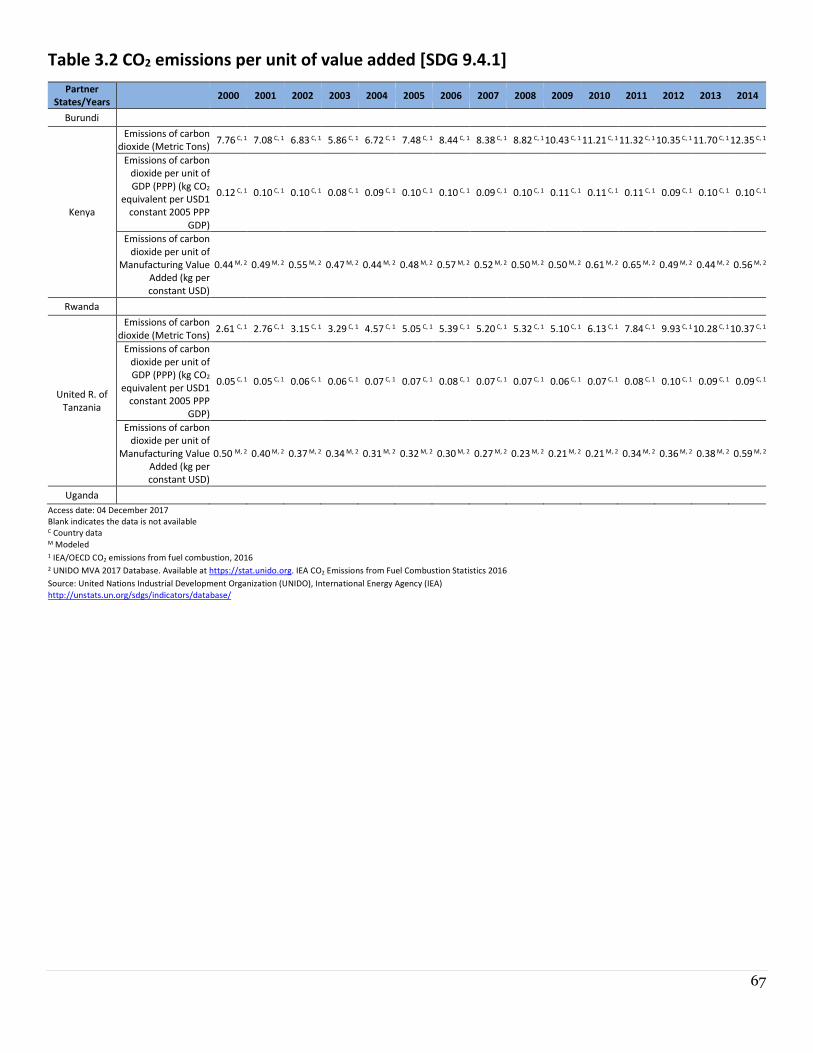
67
Table 3.2 CO2 emissions per unit of value added [SDG 9.4.1]
Partner
States/Years 2000 2001 2002 2003 2004 2005 2006 2007 2008 2009 2010 2011 2012 2013 2014
Burundi
Kenya
Emissions of carbon
dioxide (Metric Tons)7.76 C, 1 7.08 C, 1 6.83 C, 1 5.86 C, 1 6.72 C, 1 7.48 C, 1 8.44 C, 1 8.38 C, 1 8.82 C, 110.43 C, 1 11.21 C, 1 11.32 C, 1 10.35 C, 1 11.70 C, 1 12.35 C, 1
Emissions of carbon
dioxide per unit of
GDP (PPP) (kg CO2
equivalent per USD1
constant 2005 PPP
GDP)
0.12 C, 1 0.10 C, 1 0.10 C, 1 0.08 C, 1 0.09 C, 1 0.10 C, 1 0.10 C, 1 0.09 C, 1 0.10 C, 1 0.11 C, 1 0.11 C, 1 0.11 C, 1 0.09 C, 1 0.10 C, 1 0.10 C, 1
Emissions of carbon
dioxide per unit of
Manufacturing Value
Added (kg per
constant USD)
0.44 M, 2 0.49 M, 2 0.55 M, 2 0.47 M, 2 0.44 M, 2 0.48 M, 2 0.57 M, 2 0.52 M, 2 0.50 M, 2 0.50 M, 2 0.61 M, 2 0.65 M, 2 0.49 M, 2 0.44 M, 2 0.56 M, 2
Rwanda
United R. of
Tanzania
Emissions of carbon
dioxide (Metric Tons)2.61 C, 1 2.76 C, 1 3.15 C, 1 3.29 C, 1 4.57 C, 1 5.05 C, 1 5.39 C, 1 5.20 C, 1 5.32 C, 1 5.10 C, 1 6.13 C, 1 7.84 C, 1 9.93 C, 110.28 C, 1 10.37 C, 1
Emissions of carbon
dioxide per unit of
GDP (PPP) (kg CO2
equivalent per USD1
constant 2005 PPP
GDP)
0.05 C, 1 0.05 C, 1 0.06 C, 1 0.06 C, 1 0.07 C, 1 0.07 C, 1 0.08 C, 1 0.07 C, 1 0.07 C, 1 0.06 C, 1 0.07 C, 1 0.08 C, 1 0.10 C, 1 0.09 C, 1 0.09 C, 1
Emissions of carbon
dioxide per unit of
Manufacturing Value
Added (kg per
constant USD)
0.50 M, 2 0.40 M, 2 0.37 M, 2 0.34 M, 2 0.31 M, 2 0.32 M, 2 0.30 M, 2 0.27 M, 2 0.23 M, 2 0.21 M, 2 0.21 M, 2 0.34 M, 2 0.36 M, 2 0.38 M, 2 0.59 M, 2
Uganda
Access date: 04 December 2017
Blank indicates the data is not available C Country data M Modeled 1 IEA/OECD CO2 emissions from fuel combustion, 2016 2 UNIDO MVA 2017 Database. Available at https://stat.unido.org. IEA CO2 Emissions from Fuel Combustion Statistics 2016 Source: United Nations Industrial Development Organization (UNIDO), International Energy Agency (IEA)
http://unstats.un.org/sdgs/indicators/database/
68
Metadata for Table 3.2
Definition
The data in Table 3.2 shows the emissions of CO2 in tonnes, per unit of GDP in kg CO2 equivalent per USD1 constant 2005 PPP GDP,
and per unit of manufacturing value added in kg per constant USD.
Relevance
The indicator CO2 emissions per unit of value added represents the amount of emissions from fuel combustion produced by an
economic activity, per unit of economic output. When computed for the whole economy, it combines effects of the average carbon
intensity of the energy mix (linked to the shares of the various fossil fuels in the total); of the structure of an economy (linked to
the relative weight of more or less energy-intensive sectors); of the average efficiency in the use of energy. When computed for
the manufacturing sector (CO2 emissions from fuel combustion per unit of manufacturing value added), it measures the carbon
intensity of the manufacturing economic output, and its trends result from changes in the average carbon intensity of the energy
mix used, in the structure of the manufacturing sector, in the energy efficiency of production technologies in each sub-sector, and
in the economic value of the various output. Manufacturing industries are generally improving their emission intensity as countries
move to higher levels of industrialization, but it should be noted that emission intensities can also be reduced through structural
changes and product diversification in manufacturing. CO2 emission accounts for around 80% of all GHG emission from the
manufacturing processes.
Computation/Collection Method
CO2 emissions from fuel combustion are estimated based on energy consumption and on the Intergovernmental Panel on Climate
Change (IPCC) Guidelines. The total intensity of the economy is defined as the ratio of total CO2 emissions from fuel combustion
and GDP. The sectoral intensity is defined as CO2 emission from manufacturing (in physical measurement unit such as tonnes)
divided by manufacturing value added (MVA) in constant 2010 USD.
Source
UNIDO, UNSD, IEA, NSOs, https://unstats.un.org/sdgs/metadata/files/Metadata-09-04-01.pdf
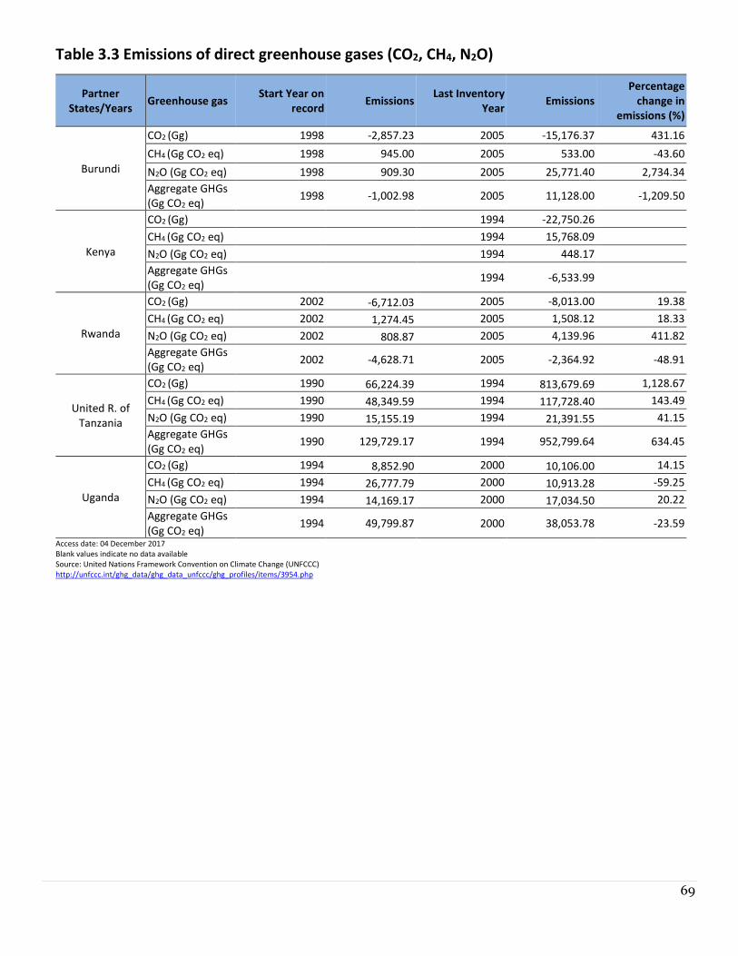
69
Table 3.3 Emissions of direct greenhouse gases (CO2, CH4, N2O)
Partner
States/Years Greenhouse gas
Start Year on
record Emissions
Last Inventory
Year Emissions
Percentage
change in
emissions (%)
Burundi
CO2 (Gg) 1998 -2,857.23 2005 -15,176.37 431.16
CH4 (Gg CO2 eq) 1998 945.00 2005 533.00 -43.60
N2O (Gg CO2 eq) 1998 909.30 2005 25,771.40 2,734.34
Aggregate GHGs
(Gg CO2 eq) 1998 -1,002.98 2005 11,128.00 -1,209.50
Kenya
CO2 (Gg) 1994 -22,750.26
CH4 (Gg CO2 eq) 1994 15,768.09
N2O (Gg CO2 eq) 1994 448.17
Aggregate GHGs
(Gg CO2 eq) 1994 -6,533.99
Rwanda
CO2 (Gg) 2002 -6,712.03 2005 -8,013.00 19.38
CH4 (Gg CO2 eq) 2002 1,274.45 2005 1,508.12 18.33
N2O (Gg CO2 eq) 2002 808.87 2005 4,139.96 411.82
Aggregate GHGs
(Gg CO2 eq) 2002 -4,628.71 2005 -2,364.92 -48.91
United R. of
Tanzania
CO2 (Gg) 1990 66,224.39 1994 813,679.69 1,128.67
CH4 (Gg CO2 eq) 1990 48,349.59 1994 117,728.40 143.49
N2O (Gg CO2 eq) 1990 15,155.19 1994 21,391.55 41.15
Aggregate GHGs
(Gg CO2 eq) 1990 129,729.17 1994 952,799.64 634.45
Uganda
CO2 (Gg) 1994 8,852.90 2000 10,106.00 14.15
CH4 (Gg CO2 eq) 1994 26,777.79 2000 10,913.28 -59.25
N2O (Gg CO2 eq) 1994 14,169.17 2000 17,034.50 20.22
Aggregate GHGs
(Gg CO2 eq) 1994 49,799.87 2000 38,053.78 -23.59
Access date: 04 December 2017 Blank values indicate no data available Source: United Nations Framework Convention on Climate Change (UNFCCC)
http://unfccc.int/ghg_data/ghg_data_unfccc/ghg_profiles/items/3954.php
70
Metadata for Table 3.3
Definition
The data in Table 3.3 shows the emissions of direct greenhouse gases (GHGs) including LULUCF/LUCF (Land Use, Land-Use Change
and forestry) at a start and end year plus the percentage of change in emissions between those two years. The data contains
estimates of CO2 – Carbon dioxide, CH4 – Methane, N2O – Nitrous oxide, and fluorinated gases – HFCs, PFCs, SF6.
Relevance
In order to stabilize greenhouse gas concentrations “at a level that would prevent dangerous anthropogenic (human induced)
interference with the climate system”, it is important to control the emissions of greenhouse gases. Activities in the LULUCF sector
can provide a relatively cost-effective way of offsetting emissions, either by increasing the removals of greenhouse gases from the
atmosphere (e.g. by planting trees or managing forests), or by reducing emissions (e.g. by curbing deforestation).
Computation/Collection Method
Each country submits national GHG inventories to the United Nations Framework Convention on Climate Change (UNFCCC) in
accordance with the reporting requirements adopted under the UNFCCC Reporting Guidelines.
Source
UNFCCC,
http://unfccc.int/ghg_data/ghg_data_unfccc/items/4146.php,
http://unfccc.int/ghg_data/ghg_data_unfccc/data_sources/items/3816.php,
http://unfccc.int/land_use_and_climate_change/lulucf/items/3060.php
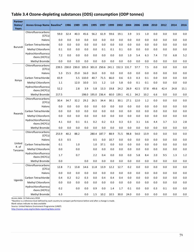
71
Table 3.4 Ozone-depleting substances (ODS) consumption (ODP tonnes)
Partner
States/
Years
Annex Group Name Baseline* 1986 1989 1991 1995 1997 1999 2002 2004 2006 2008 2010 2012 2014 2016
Burundi
Chlorofluorocarbons
(CFCs) 59.0 32.4 40.3 45.6 56.2 61.9 59.6 19.1 3.9 3.5 1.0 0.0 0.0 0.0 0.0
Halons 0.0 0.0 0.0 0.0 0.0 0.0 0.0 0.0 0.0 0.0 0.0 0.0 0.0 0.0 0.0
Carbon Tetrachloride 0.0 0.0 0.0 0.0 0.0 0.0 0.0 0.0 0.0 0.0 0.0 0.0 0.0 0.0 0.0
Methyl Chloroform 0.1 0.0 0.0 0.0 0.0 0.1 0.1 0.1 0.0 0.0 0.0 0.0 0.0 0.0 0.0
Hydrochlorofluoroca
rbons (HCFCs) 7.2 0.0 0.0 0.0 0.0 0.0 0.0 0.0 1.0 5.4 6.3 7.4 7.0 6.8 5.2
Methyl Bromide 0.0 0.0 0.0 0.0 0.0 0.0 0.0 0.0 0.0 0.0 0.0 0.0 0.0 0.0 0.0
Kenya
Chlorofluorocarbons
(CFCs) 239.5 230.0 230.0 105.0 301.0 250.6 241.1 152.3 131.7 57.7 7.5 0.0 0.0 0.0 0.0
Halons 5.3 15.5 25.0 16.0 16.0 0.0 0.0 0.0 0.0 0.0 0.0 0.0 0.0 0.0 0.0
Carbon Tetrachloride 65.9 5.5 110.0 40.7 71.5 66.0 0.6 0.3 0.3 0.1 0.0 0.0 0.0 0.0
Methyl Chloroform 1.1 12.0 10.0 3.5 1.2 1.0 5.8 0.0 0.1 0.1 0.0 0.0 0.0 0.0
Hydrochlorofluoroca
rbons (HCFCs) 52.2 2.8 3.9 5.8 13.3 19.8 24.2 26.9 42.5 57.8 49.6 42.4 24.8 15.1
Methyl Bromide 217.5 198.0 195.0 236.4 60.0 139.1 41.1 34.2 10.2 6.6 0.0 0.0 0.0
Rwanda
Chlorofluorocarbons
(CFCs) 30.4 34.7 32.2 29.2 26.5 34.4 30.1 30.1 27.1 12.0 1.2 0.0 0.0 0.0 0.0
Halons 0.0 0.0 0.0 0.0 0.0 0.0 0.0 0.0 0.0 0.0 0.0 0.0 0.0 0.0 0.0
Carbon Tetrachloride 0.0 0.0 0.0 0.0 0.0 0.0 0.0 0.0 0.0 0.0 0.0 0.0 0.0 0.0 0.0
Methyl Chloroform 0.0 0.0 0.0 0.0 0.0 0.0 0.0 0.0 0.0 0.0 0.0 0.0 0.0 0.0 0.0
Hydrochlorofluoroca
rbons (HCFCs) 4.1 0.0 0.1 0.1 0.2 0.2 0.3 0.3 0.3 3.1 3.6 4.4 3.7 3.3 2.8
Methyl Bromide 0.0 0.0 0.0 0.0 0.0 0.0 0.0 0.0 0.0 0.0 0.0 0.0 0.0 0.0 0.0
United
R. of
Tanzania
Chlorofluorocarbons
(CFCs) 253.9 40.2 88.2 280.4 187.7 88.9 71.5 98.8 54.0 13.9 0.0 0.0 0.0 0.0
Halons 0.3 0.5 0.5 0.0 10.7 0.0 0.0 0.0 0.0 0.0 0.0 0.0 0.0
Carbon Tetrachloride 0.1 1.0 1.0 37.1 0.0 0.0 0.0 0.0 0.0 0.0 0.0 0.0 0.0
Methyl Chloroform 0.0 0.0 0.0 0.0 0.0 0.0 0.0 0.0 0.0 0.0 0.0 0.0 0.0
Hydrochlorofluoroca
rbons (HCFCs) 1.7 0.7 2.2 0.4 0.0 0.0 0.0 5.8 8.4 2.0 9.5 1.3 1.2
Methyl Bromide 0.0 0.0 0.0 0.0 0.0 0.0 0.0 0.0 0.0 0.0 0.0 0.0 0.0
Uganda
Chlorofluorocarbons
(CFCs) 12.8 7.1 13.8 14.6 11.8 13.9 12.2 12.7 0.2 0.0 0.0 0.0 0.0 0.0 0.0
Halons 0.0 0.0 0.0 0.0 0.0 0.0 0.0 0.0 0.0 0.0 0.0 0.0 0.0 0.0 0.0
Carbon Tetrachloride 0.4 0.2 0.2 0.3 0.0 0.4 0.4 0.4 0.0 0.0 0.0 0.0 0.0 0.0 0.0
Methyl Chloroform 0.0 0.0 0.0 0.0 0.0 0.0 0.0 0.0 0.0 0.0 0.0 0.0 0.0 0.0 0.0
Hydrochlorofluoroca
rbons (HCFCs) 0.2 0.0 0.0 0.9 0.0 1.4 1.7 0.1 0.0 0.0 0.3 0.1 0.0 0.0
Methyl Bromide 6.3 0.0 1.5 10.2 10.5 30.0 24.0 0.0 0.0 0.0 0.0 0.0 0.0
Access date: 12 Februrary 2018 *Baseline is a reference level defined by each country to compare performance before and after a change is made.
Blank values indicate no data available
Source: United Nations Enviroment Programme (UNEP)
http://ozone.unep.org/en/data-reporting/data-centre
72
Metadata for Table 3.4
Definition
This indicator is used to monitor the reduction in the usage of Ozone Depleting Substances (ODSs) as a result of the Montreal
Protocol. Therefore, only ODSs controlled under the Montreal Protocol are covered by the indicator. Reducing consumption
ultimately leads to reductions in emissions since most uses of ODSs finally lead to the substances being emitted into the
atmosphere. The units of measurement are metric tons of ODS weighted by their Ozone Depletion Potential (ODP), otherwise
referred to as ODP tons.
Relevance
Ozone depleting substances (ODSs) is any substance containing chlorine or bromine, which destroys the stratospheric ozone layer
that absorbs most of the biologically damaging ultraviolet radiation. The phasing out of ozone depleting substances, and their
substitution by less harmful substances or new processes, are aimed at the recovery of the ozone layer.
Computation/Collection Method
Parties report their Production, Imports, Exports and Destruction of individual substances controlled under the Montreal Protocol
in metric tonnes. For each substance, the metric tonnes are then multiplied by the ODP of the substance (resulting in ODP-
weighted tonnes, or in short ODP-tonnes).
Consumption is then calculated as production plus imports minus exports minus destroyed quantities minus feedstock uses of a
controlled substance. Destruction and feedstock uses both take out ODS out of the system (opposite of production), hence the
reason for subtracting them when calculating consumption. The Protocol also specifies that consumption shall not include the
amounts used for quarantine and pre-shipment applications of methyl bromide, and further specifies that exports to non-Parties
will count as consumption in the exporting Party.
The precise formula for calculating consumption is:
consumption = total production - destroyed - production for internal feedstock use - production for internal quarantine use (for
methyl bromide only) + total new imports - import for feedstock - import for quarantine use – total new exports + export to non-
parties.
Source
UNSD, http://mdgs.un.org/unsd/mdg/Metadata.aspx
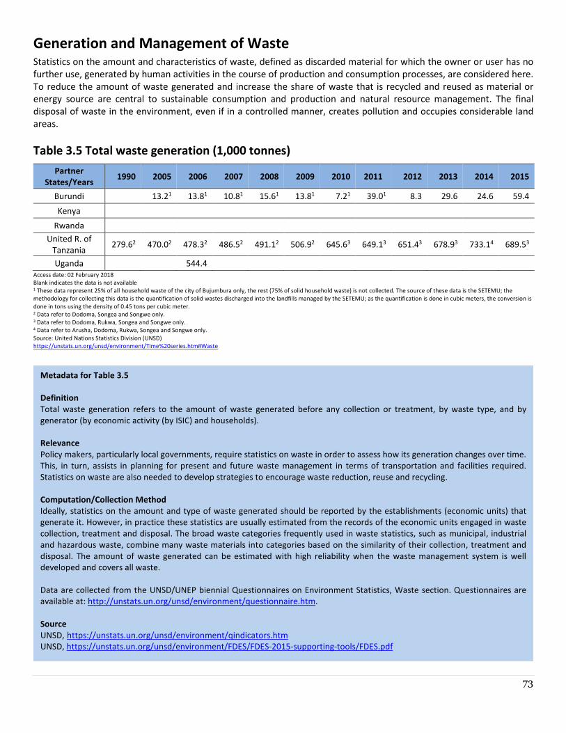
73
Generation and Management of Waste Statistics on the amount and characteristics of waste, defined as discarded material for which the owner or user has no
further use, generated by human activities in the course of production and consumption processes, are considered here.
To reduce the amount of waste generated and increase the share of waste that is recycled and reused as material or
energy source are central to sustainable consumption and production and natural resource management. The final
disposal of waste in the environment, even if in a controlled manner, creates pollution and occupies considerable land
areas.
Table 3.5 Total waste generation (1,000 tonnes)
Partner
States/Years 1990 2005 2006 2007 2008 2009 2010 2011 2012 2013 2014 2015
Burundi 13.21 13.81 10.81 15.61 13.81 7.21 39.01 8.3 29.6 24.6 59.4
Kenya
Rwanda
United R. of
Tanzania 279.62 470.02 478.32 486.52 491.12 506.92 645.63 649.13 651.43 678.93 733.14 689.53
Uganda 544.4 Access date: 02 February 2018
Blank indicates the data is not available 1 These data represent 25% of all household waste of the city of Bujumbura only, the rest (75% of solid household waste) is not collected. The source of these data is the SETEMU; the
methodology for collecting this data is the quantification of solid wastes discharged into the landfills managed by the SETEMU; as the quantification is done in cubic meters, the conversion is
done in tons using the density of 0.45 tons per cubic meter. 2 Data refer to Dodoma, Songea and Songwe only. 3 Data refer to Dodoma, Rukwa, Songea and Songwe only. 4 Data refer to Arusha, Dodoma, Rukwa, Songea and Songwe only.
Source: United Nations Statistics Division (UNSD)
https://unstats.un.org/unsd/environment/Time%20series.htm#Waste
Metadata for Table 3.5
Definition
Total waste generation refers to the amount of waste generated before any collection or treatment, by waste type, and by
generator (by economic activity (by ISIC) and households).
Relevance
Policy makers, particularly local governments, require statistics on waste in order to assess how its generation changes over time.
This, in turn, assists in planning for present and future waste management in terms of transportation and facilities required.
Statistics on waste are also needed to develop strategies to encourage waste reduction, reuse and recycling.
Computation/Collection Method
Ideally, statistics on the amount and type of waste generated should be reported by the establishments (economic units) that
generate it. However, in practice these statistics are usually estimated from the records of the economic units engaged in waste
collection, treatment and disposal. The broad waste categories frequently used in waste statistics, such as municipal, industrial
and hazardous waste, combine many waste materials into categories based on the similarity of their collection, treatment and
disposal. The amount of waste generated can be estimated with high reliability when the waste management system is well
developed and covers all waste.
Data are collected from the UNSD/UNEP biennial Questionnaires on Environment Statistics, Waste section. Questionnaires are
available at: http://unstats.un.org/unsd/environment/questionnaire.htm.
Source
UNSD, https://unstats.un.org/unsd/environment/qindicators.htm
UNSD, https://unstats.un.org/unsd/environment/FDES/FDES-2015-supporting-tools/FDES.pdf
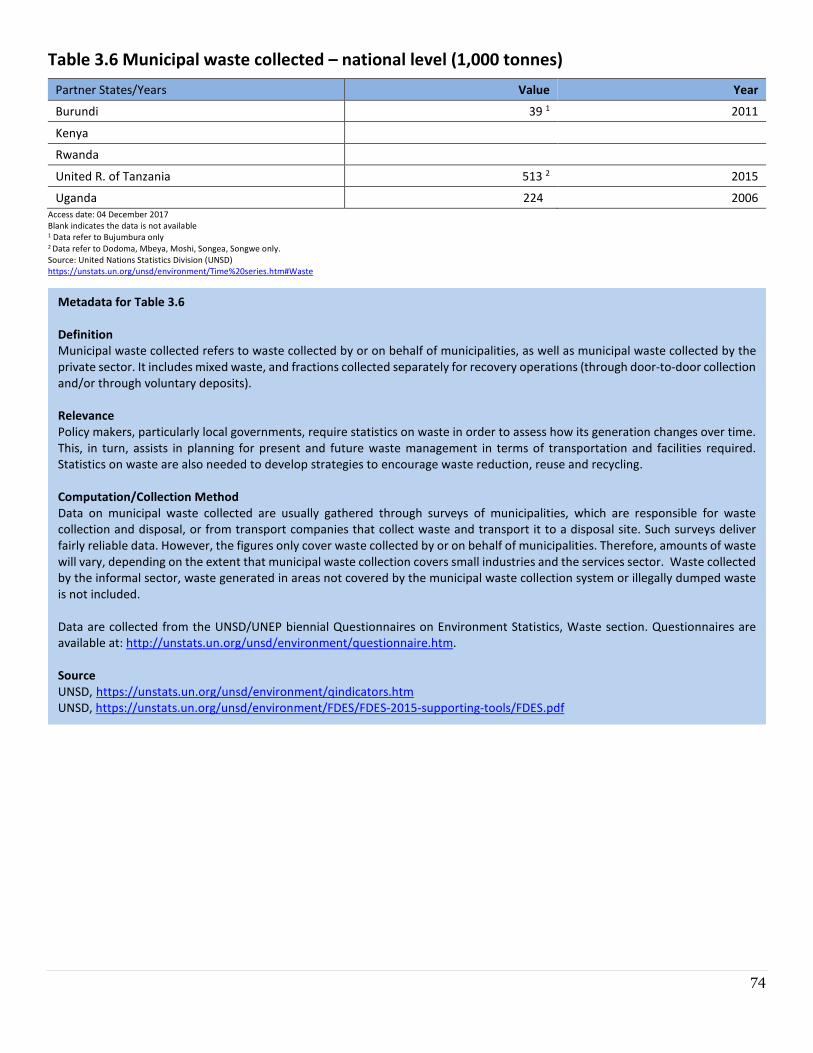
74
Table 3.6 Municipal waste collected – national level (1,000 tonnes)
Partner States/Years Value Year
Burundi 39 1 2011
Kenya
Rwanda
United R. of Tanzania 513 2 2015
Uganda 224 2006
Access date: 04 December 2017
Blank indicates the data is not available 1 Data refer to Bujumbura only 2 Data refer to Dodoma, Mbeya, Moshi, Songea, Songwe only.
Source: United Nations Statistics Division (UNSD)
https://unstats.un.org/unsd/environment/Time%20series.htm#Waste
Metadata for Table 3.6
Definition
Municipal waste collected refers to waste collected by or on behalf of municipalities, as well as municipal waste collected by the
private sector. It includes mixed waste, and fractions collected separately for recovery operations (through door-to-door collection
and/or through voluntary deposits).
Relevance
Policy makers, particularly local governments, require statistics on waste in order to assess how its generation changes over time.
This, in turn, assists in planning for present and future waste management in terms of transportation and facilities required.
Statistics on waste are also needed to develop strategies to encourage waste reduction, reuse and recycling.
Computation/Collection Method
Data on municipal waste collected are usually gathered through surveys of municipalities, which are responsible for waste
collection and disposal, or from transport companies that collect waste and transport it to a disposal site. Such surveys deliver
fairly reliable data. However, the figures only cover waste collected by or on behalf of municipalities. Therefore, amounts of waste
will vary, depending on the extent that municipal waste collection covers small industries and the services sector. Waste collected
by the informal sector, waste generated in areas not covered by the municipal waste collection system or illegally dumped waste
is not included.
Data are collected from the UNSD/UNEP biennial Questionnaires on Environment Statistics, Waste section. Questionnaires are
available at: http://unstats.un.org/unsd/environment/questionnaire.htm.
Source
UNSD, https://unstats.un.org/unsd/environment/qindicators.htm
UNSD, https://unstats.un.org/unsd/environment/FDES/FDES-2015-supporting-tools/FDES.pdf
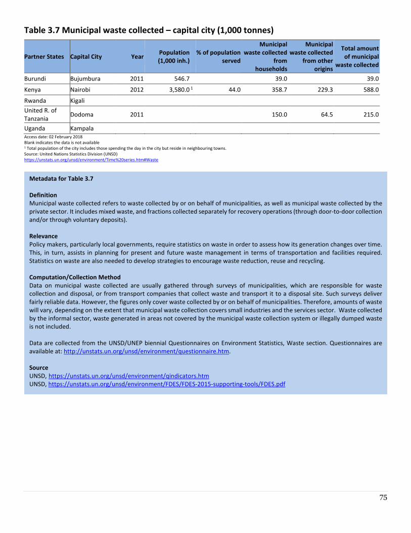
75
Table 3.7 Municipal waste collected – capital city (1,000 tonnes)
Partner States Capital City Year Population
(1,000 inh.)
% of population
served
Municipal
waste collected
from
households
Municipal
waste collected
from other
origins
Total amount
of municipal
waste collected
Burundi Bujumbura 2011 546.7 39.0 39.0
Kenya Nairobi 2012 3,580.0 1 44.0 358.7 229.3 588.0
Rwanda Kigali
United R. of
Tanzania Dodoma 2011
150.0 64.5 215.0
Uganda Kampala
Access date: 02 February 2018
Blank indicates the data is not available 1 Total population of the city includes those spending the day in the city but reside in neighbouring towns.
Source: United Nations Statistics Division (UNSD)
https://unstats.un.org/unsd/environment/Time%20series.htm#Waste
Metadata for Table 3.7
Definition
Municipal waste collected refers to waste collected by or on behalf of municipalities, as well as municipal waste collected by the
private sector. It includes mixed waste, and fractions collected separately for recovery operations (through door-to-door collection
and/or through voluntary deposits).
Relevance
Policy makers, particularly local governments, require statistics on waste in order to assess how its generation changes over time.
This, in turn, assists in planning for present and future waste management in terms of transportation and facilities required.
Statistics on waste are also needed to develop strategies to encourage waste reduction, reuse and recycling.
Computation/Collection Method
Data on municipal waste collected are usually gathered through surveys of municipalities, which are responsible for waste
collection and disposal, or from transport companies that collect waste and transport it to a disposal site. Such surveys deliver
fairly reliable data. However, the figures only cover waste collected by or on behalf of municipalities. Therefore, amounts of waste
will vary, depending on the extent that municipal waste collection covers small industries and the services sector. Waste collected
by the informal sector, waste generated in areas not covered by the municipal waste collection system or illegally dumped waste
is not included.
Data are collected from the UNSD/UNEP biennial Questionnaires on Environment Statistics, Waste section. Questionnaires are
available at: http://unstats.un.org/unsd/environment/questionnaire.htm.
Source
UNSD, https://unstats.un.org/unsd/environment/qindicators.htm
UNSD, https://unstats.un.org/unsd/environment/FDES/FDES-2015-supporting-tools/FDES.pdf
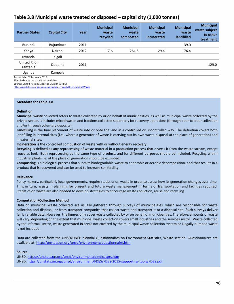
76
Table 3.8 Municipal waste treated or disposed – capital city (1,000 tonnes)
Partner States Capital City Year
Municipal
waste
recycled
Municipal
waste
composted
Municipal
waste
incinerated
Municipal
waste
landfilled
Municipal
waste subject
to other
treatment
Burundi Bujumbura 2011 39.0
Kenya Nairobi 2012 117.6 264.6 29.4 176.4
Rwanda Kigali
United R. of
Tanzania Dodoma 2011 129.0
Uganda Kampala Access date: 02 February 2018
Blank indicates the data is not available
Source: United Nations Statistics Division (UNSD)
https://unstats.un.org/unsd/environment/Time%20series.htm#Waste
Metadata for Table 3.8
Definition
Municipal waste collected refers to waste collected by or on behalf of municipalities, as well as municipal waste collected by the
private sector. It includes mixed waste, and fractions collected separately for recovery operations (through door-to-door collection
and/or through voluntary deposits).
Landfilling is the final placement of waste into or onto the land in a controlled or uncontrolled way. The definition covers both
landfilling in internal sites (i.e., where a generator of waste is carrying out its own waste disposal at the place of generation) and
in external sites.
Incineration is the controlled combustion of waste with or without energy recovery.
Recycling is defined as any reprocessing of waste material in a production process that diverts it from the waste stream, except
reuse as fuel. Both reprocessing as the same type of product, and for different purposes should be included. Recycling within
industrial plants i.e. at the place of generation should be excluded.
Composting is a biological process that submits biodegradable waste to anaerobic or aerobic decomposition, and that results in a
product that is recovered and can be used to increase soil fertility.
Relevance
Policy makers, particularly local governments, require statistics on waste in order to assess how its generation changes over time.
This, in turn, assists in planning for present and future waste management in terms of transportation and facilities required.
Statistics on waste are also needed to develop strategies to encourage waste reduction, reuse and recycling.
Computation/Collection Method
Data on municipal waste collected are usually gathered through surveys of municipalities, which are responsible for waste
collection and disposal, or from transport companies that collect waste and transport it to a disposal site. Such surveys deliver
fairly reliable data. However, the figures only cover waste collected by or on behalf of municipalities. Therefore, amounts of waste
will vary, depending on the extent that municipal waste collection covers small industries and the services sector. Waste collected
by the informal sector, waste generated in areas not covered by the municipal waste collection system or illegally dumped waste
is not included.
Data are collected from the UNSD/UNEP biennial Questionnaires on Environment Statistics, Waste section. Questionnaires are
available at: http://unstats.un.org/unsd/environment/questionnaire.htm.
Source
UNSD, https://unstats.un.org/unsd/environment/qindicators.htm
UNSD, https://unstats.un.org/unsd/environment/FDES/FDES-2015-supporting-tools/FDES.pdf
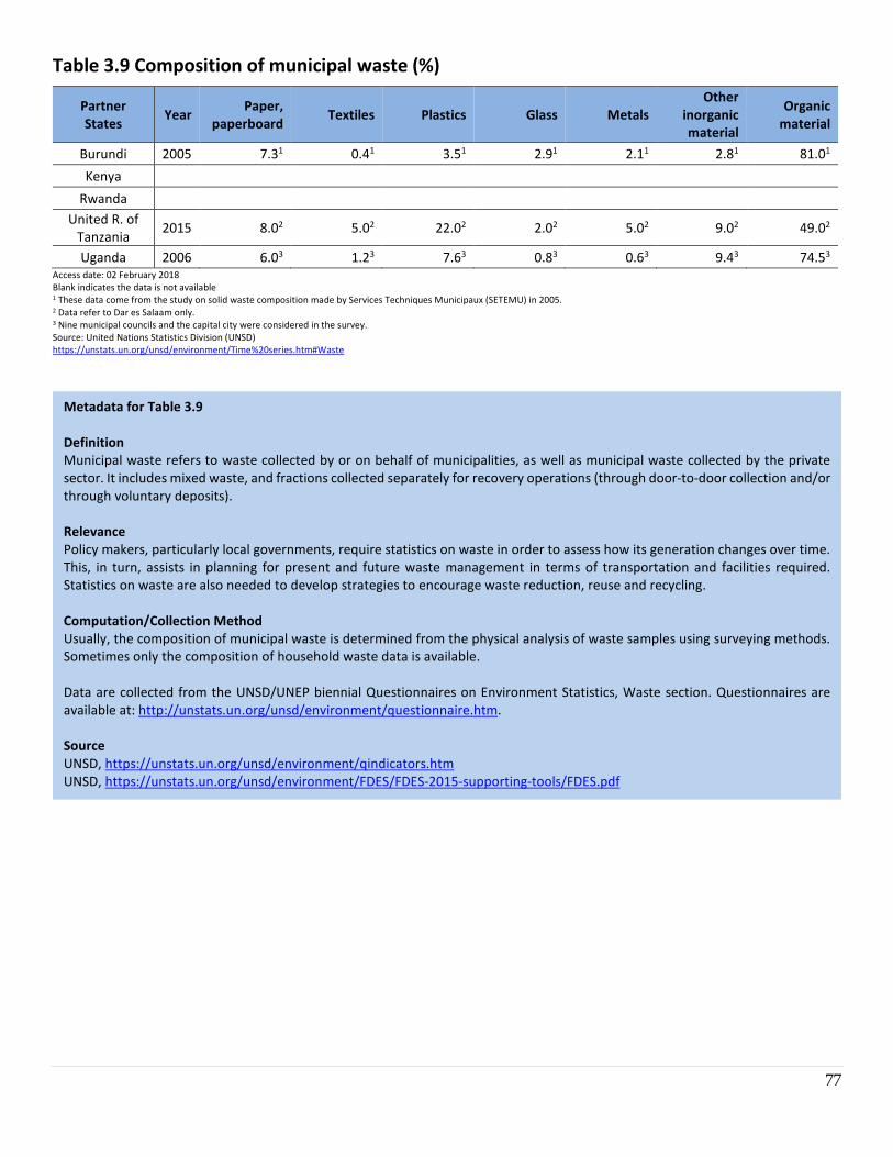
77
Table 3.9 Composition of municipal waste (%)
Partner
States Year
Paper,
paperboard Textiles Plastics Glass Metals
Other
inorganic
material
Organic
material
Burundi 2005 7.31 0.41 3.51 2.91 2.11 2.81 81.01
Kenya
Rwanda
United R. of
Tanzania 2015 8.02 5.02 22.02 2.02 5.02 9.02 49.02
Uganda 2006 6.03 1.23 7.63 0.83 0.63 9.43 74.53
Access date: 02 February 2018
Blank indicates the data is not available 1 These data come from the study on solid waste composition made by Services Techniques Municipaux (SETEMU) in 2005. 2 Data refer to Dar es Salaam only. 3 Nine municipal councils and the capital city were considered in the survey.
Source: United Nations Statistics Division (UNSD)
https://unstats.un.org/unsd/environment/Time%20series.htm#Waste
Metadata for Table 3.9
Definition
Municipal waste refers to waste collected by or on behalf of municipalities, as well as municipal waste collected by the private
sector. It includes mixed waste, and fractions collected separately for recovery operations (through door-to-door collection and/or
through voluntary deposits).
Relevance
Policy makers, particularly local governments, require statistics on waste in order to assess how its generation changes over time.
This, in turn, assists in planning for present and future waste management in terms of transportation and facilities required.
Statistics on waste are also needed to develop strategies to encourage waste reduction, reuse and recycling.
Computation/Collection Method
Usually, the composition of municipal waste is determined from the physical analysis of waste samples using surveying methods.
Sometimes only the composition of household waste data is available.
Data are collected from the UNSD/UNEP biennial Questionnaires on Environment Statistics, Waste section. Questionnaires are
available at: http://unstats.un.org/unsd/environment/questionnaire.htm.
Source
UNSD, https://unstats.un.org/unsd/environment/qindicators.htm
UNSD, https://unstats.un.org/unsd/environment/FDES/FDES-2015-supporting-tools/FDES.pdf
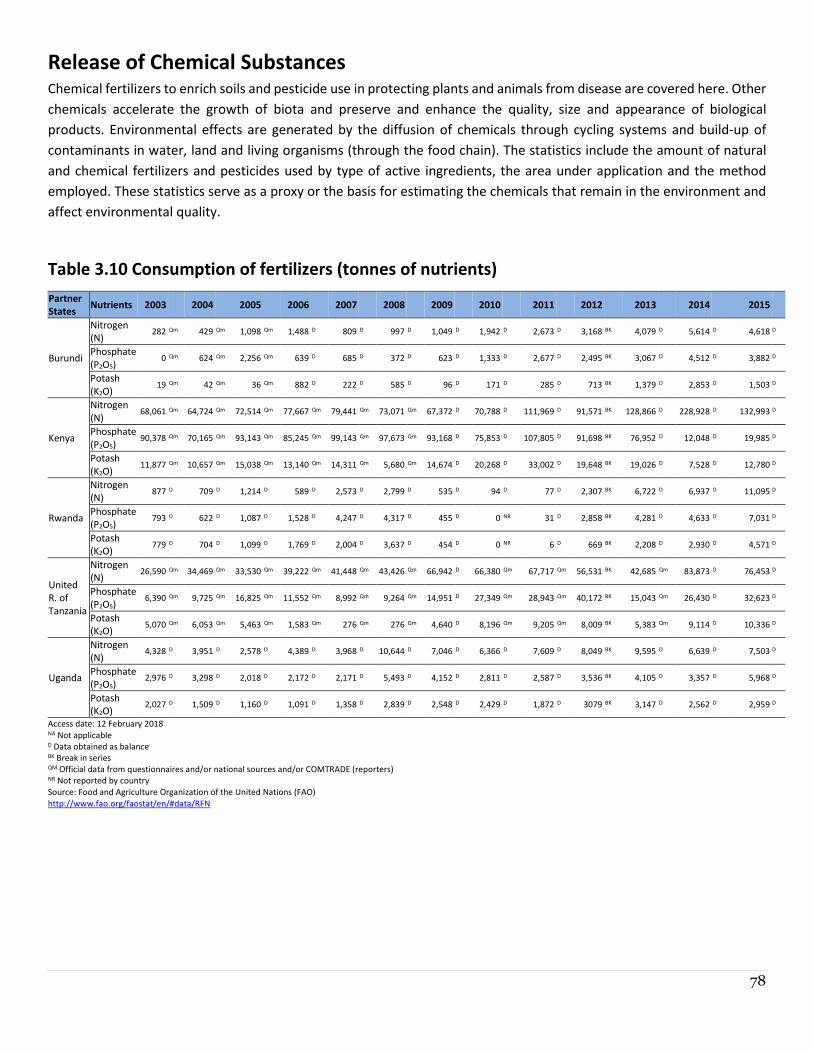
78
Release of Chemical Substances Chemical fertilizers to enrich soils and pesticide use in protecting plants and animals from disease are covered here. Other
chemicals accelerate the growth of biota and preserve and enhance the quality, size and appearance of biological
products. Environmental effects are generated by the diffusion of chemicals through cycling systems and build-up of
contaminants in water, land and living organisms (through the food chain). The statistics include the amount of natural
and chemical fertilizers and pesticides used by type of active ingredients, the area under application and the method
employed. These statistics serve as a proxy or the basis for estimating the chemicals that remain in the environment and
affect environmental quality.
Table 3.10 Consumption of fertilizers (tonnes of nutrients)
Partner
States Nutrients 2003 2004 2005 2006 2007 2008 2009 2010 2011 2012 2013 2014 2015
Burundi
Nitrogen
(N) 282 Qm 429 Qm 1,098 Qm 1,488 D 809 D 997 D 1,049 D 1,942 D 2,673 D 3,168 BK 4,079 D 5,614 D 4,618 D
Phosphate
(P2O5) 0 Qm 624 Qm 2,256 Qm 639 D 685 D 372 D 623 D 1,333 D 2,677 D 2,495 BK 3,067 D 4,512 D 3,882 D
Potash
(K2O) 19 Qm 42 Qm 36 Qm 882 D 222 D 585 D 96 D 171 D 285 D 713 BK 1,379 D 2,853 D 1,503 D
Kenya
Nitrogen
(N) 68,061 Qm 64,724 Qm 72,514 Qm 77,667 Qm 79,441 Qm 73,071 Qm 67,372 D 70,788 D 111,969 D 91,571 BK 128,866 D 228,928 D 132,993 D
Phosphate
(P2O5) 90,378 Qm 70,165 Qm 93,143 Qm 85,245 Qm 99,143 Qm 97,673 Qm 93,168 D 75,853 D 107,805 D 91,698 BK 76,952 D 12,048 D 19,985 D
Potash
(K2O) 11,877 Qm 10,657 Qm 15,038 Qm 13,140 Qm 14,311 Qm 5,680 Qm 14,674 D 20,268 D 33,002 D 19,648 BK 19,026 D 7,528 D 12,780 D
Rwanda
Nitrogen
(N) 877 D 709 D 1,214 D 589 D 2,573 D 2,799 D 535 D 94 D 77 D 2,307 BK 6,722 D 6,937 D 11,095 D
Phosphate
(P2O5) 793 D 622 D 1,087 D 1,528 D 4,247 D 4,317 D 455 D 0 NR 31 D 2,858 BK 4,281 D 4,633 D 7,031 D
Potash
(K2O) 779 D 704 D 1,099 D 1,769 D 2,004 D 3,637 D 454 D 0 NR 6 D 669 BK 2,208 D 2,930 D 4,571 D
United
R. of
Tanzania
Nitrogen
(N) 26,590 Qm 34,469 Qm 33,530 Qm 39,222 Qm 41,448 Qm 43,426 Qm 66,942 D 66,380 Qm 67,717 Qm 56,531 BK 42,685 Qm 83,873 D 76,453 D
Phosphate
(P2O5) 6,390 Qm 9,725 Qm 16,825 Qm 11,552 Qm 8,992 Qm 9,264 Qm 14,951 D 27,349 Qm 28,943 Qm 40,172 BK 15,043 Qm 26,430 D 32,623 D
Potash
(K2O) 5,070 Qm 6,053 Qm 5,463 Qm 1,583 Qm 276 Qm 276 Qm 4,640 D 8,196 Qm 9,205 Qm 8,009 BK 5,383 Qm 9,114 D 10,336 D
Uganda
Nitrogen
(N) 4,328 D 3,951 D 2,578 D 4,389 D 3,968 D 10,644 D 7,046 D 6,366 D 7,609 D 8,049 BK 9,595 D 6,639 D 7,503 D
Phosphate
(P2O5) 2,976 D 3,298 D 2,018 D 2,172 D 2,171 D 5,493 D 4,152 D 2,811 D 2,587 D 3,536 BK 4,105 D 3,357 D 5,968 D
Potash
(K2O) 2,027 D 1,509 D 1,160 D 1,091 D 1,358 D 2,839 D 2,548 D 2,429 D 1,872 D 3079 BK 3,147 D 2,562 D 2,959 D
Access date: 12 February 2018 NA Not applicable D Data obtained as balance BK Break in series QM Official data from questionnaires and/or national sources and/or COMTRADE (reporters) NR Not reported by country
Source: Food and Agriculture Organization of the United Nations (FAO)
http://www.fao.org/faostat/en/#data/RFN
79
Metadata for Table 3.10
Definition
Table 3.10 shows annual consumption of fertilizers for the three main plant nutrients: nitrogen (N), phosphate (P2O5), potash (K2O)
expressed in tonnes.
Relevance
These statistics are useful for market management and monitoring, production forecasts and policy-making in agricultural and
food sectors.
Computation/Collection Method
Fertilizer consumption data is calculated based on the equation:
C = A+O
Where:
C = fertilizers Consumption
A = Agricultural use
O = Other uses
Countries report to FAO data on A and O through the FAOSTAT Fertilizers questionnaire.
Source
FAO, http://fenixservices.fao.org/faostat/static/documents/RF/RF_e.pdf
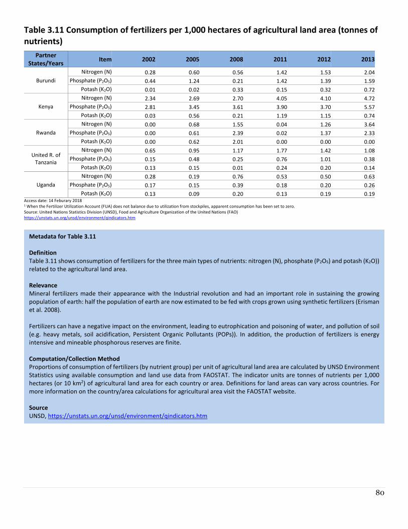
80
Table 3.11 Consumption of fertilizers per 1,000 hectares of agricultural land area (tonnes of
nutrients)
Partner
States/Years Item 2002 2005 2008 2011 2012 2013
Burundi
Nitrogen (N) 0.28 0.60 0.56 1.42 1.53 2.04
Phosphate (P2O5) 0.44 1.24 0.21 1.42 1.39 1.59
Potash (K2O) 0.01 0.02 0.33 0.15 0.32 0.72
Kenya
Nitrogen (N) 2.34 2.69 2.70 4.05 4.10 4.72
Phosphate (P2O5) 2.81 3.45 3.61 3.90 3.70 5.57
Potash (K2O) 0.03 0.56 0.21 1.19 1.15 0.74
Rwanda
Nitrogen (N) 0.00 0.68 1.55 0.04 1.26 3.64
Phosphate (P2O5) 0.00 0.61 2.39 0.02 1.37 2.33
Potash (K2O) 0.00 0.62 2.01 0.00 0.00 0.00
United R. of
Tanzania
Nitrogen (N) 0.65 0.95 1.17 1.77 1.42 1.08
Phosphate (P2O5) 0.15 0.48 0.25 0.76 1.01 0.38
Potash (K2O) 0.13 0.15 0.01 0.24 0.20 0.14
Uganda
Nitrogen (N) 0.28 0.19 0.76 0.53 0.50 0.63
Phosphate (P2O5) 0.17 0.15 0.39 0.18 0.20 0.26
Potash (K2O) 0.13 0.09 0.20 0.13 0.19 0.19Access date: 14 Feburary 2018 1 When the Fertilizer Utilization Account (FUA) does not balance due to utilization from stockpiles, apparent consumption has been set to zero.
Source: United Nations Statistics Division (UNSD), Food and Agriculture Organization of the United Nations (FAO)
https://unstats.un.org/unsd/environment/qindicators.htm
Metadata for Table 3.11
Definition
Table 3.11 shows consumption of fertilizers for the three main types of nutrients: nitrogen (N), phosphate (P2O5) and potash (K2O))
related to the agricultural land area.
Relevance
Mineral fertilizers made their appearance with the Industrial revolution and had an important role in sustaining the growing
population of earth: half the population of earth are now estimated to be fed with crops grown using synthetic fertilizers (Erisman
et al. 2008).
Fertilizers can have a negative impact on the environment, leading to eutrophication and poisoning of water, and pollution of soil
(e.g. heavy metals, soil acidification, Persistent Organic Pollutants (POPs)). In addition, the production of fertilizers is energy
intensive and mineable phosphorous reserves are finite.
Computation/Collection Method
Proportions of consumption of fertilizers (by nutrient group) per unit of agricultural land area are calculated by UNSD Environment
Statistics using available consumption and land use data from FAOSTAT. The indicator units are tonnes of nutrients per 1,000
hectares (or 10 km2) of agricultural land area for each country or area. Definitions for land areas can vary across countries. For
more information on the country/area calculations for agricultural area visit the FAOSTAT website.
Source
UNSD, https://unstats.un.org/unsd/environment/qindicators.htm
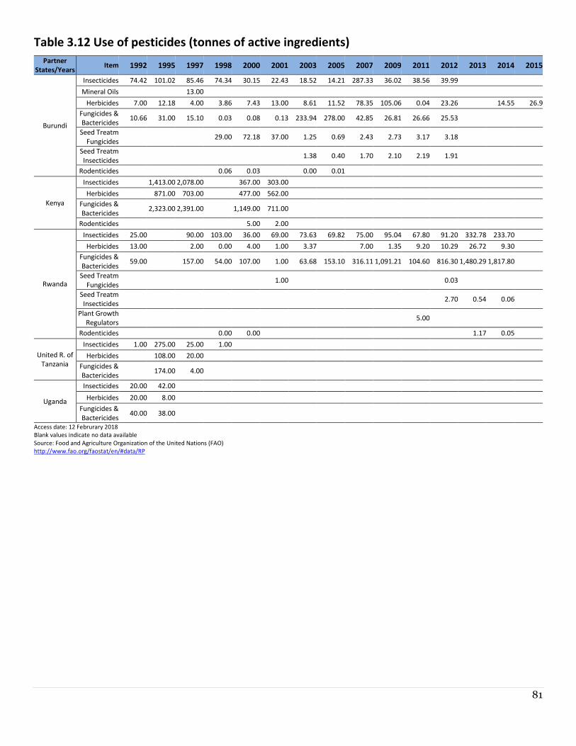
81
Table 3.12 Use of pesticides (tonnes of active ingredients)
Partner
States/Years Item 1992 1995 1997 1998 2000 2001 2003 2005 2007 2009 2011 2012 2013 2014 2015
Burundi
Insecticides 74.42 101.02 85.46 74.34 30.15 22.43 18.52 14.21 287.33 36.02 38.56 39.99
Mineral Oils 13.00
Herbicides 7.00 12.18 4.00 3.86 7.43 13.00 8.61 11.52 78.35 105.06 0.04 23.26 14.55 26.9
Fungicides &
Bactericides10.66 31.00 15.10 0.03 0.08 0.13 233.94 278.00 42.85 26.81 26.66 25.53
Seed Treatm
Fungicides29.00 72.18 37.00 1.25 0.69 2.43 2.73 3.17 3.18
Seed Treatm
Insecticides1.38 0.40 1.70 2.10 2.19 1.91
Rodenticides 0.06 0.03 0.00 0.01
Kenya
Insecticides 1,413.00 2,078.00 367.00 303.00
Herbicides 871.00 703.00 477.00 562.00
Fungicides &
Bactericides2,323.00 2,391.00 1,149.00 711.00
Rodenticides 5.00 2.00
Rwanda
Insecticides 25.00 90.00 103.00 36.00 69.00 73.63 69.82 75.00 95.04 67.80 91.20 332.78 233.70
Herbicides 13.00 2.00 0.00 4.00 1.00 3.37 7.00 1.35 9.20 10.29 26.72 9.30
Fungicides &
Bactericides59.00 157.00 54.00 107.00 1.00 63.68 153.10 316.11 1,091.21 104.60 816.30 1,480.29 1,817.80
Seed Treatm
Fungicides1.00 0.03
Seed Treatm
Insecticides2.70 0.54 0.06
Plant Growth
Regulators5.00
Rodenticides 0.00 0.00 1.17 0.05
United R. of
Tanzania
Insecticides 1.00 275.00 25.00 1.00
Herbicides 108.00 20.00
Fungicides &
Bactericides174.00 4.00
Uganda
Insecticides 20.00 42.00
Herbicides 20.00 8.00
Fungicides &
Bactericides40.00 38.00
Access date: 12 Februrary 2018
Blank values indicate no data available
Source: Food and Agriculture Organization of the United Nations (FAO)
http://www.fao.org/faostat/en/#data/RP
82
Metadata for Table 3.12
Definition
Table 3.12 shows the usage of the major pesticides that are intended for preventing, destroying or controlling any pest, including
vectors of human or animal diseases, unwanted species of plants or animals causing harm during or otherwise interfering with the
production, processing, storage, transport or marketing of food, agricultural commodities, wood and wood products or animal
feedstuffs, or substances which may be administered to animals for the control of insects, arachnids or other pests in or on their
bodies. They also include substances intended for use as a plant growth regulator, defoliant, desiccant or agent for thinning fruit
or preventing the premature fall of fruit.
Relevance
The application of and the residuals from pesticides are an environmental health concern. Residuals in soil from the use of
pesticides play an important role in determining its quality, productive capacity and pollution levels.
Computation/Collection Method
The annual FAO Questionnaire on Pesticides Use is the main source of data for this domain. These official statistics may be
complemented with government data sources such as yearbooks and ministerial data portals. Data gaps may be filled with
secondary sources such as country studies from other international organizations.
Source
FAO, http://www.fao.org/faostat/en/#data/RP/metadata

83

84
Chapter 4
Natural Extreme Events and Disasters
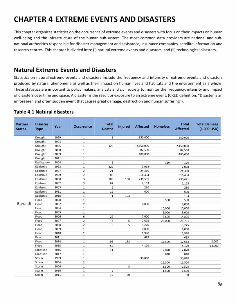
85
CHAPTER 4 EXTREME EVENTS AND DISASTERS
This chapter organizes statistics on the occurrence of extreme events and disasters with focus on their impacts on human
well-being and the infrastructure of the human sub-system. The most common data providers are national and sub-
national authorities responsible for disaster management and assistance, insurance companies, satellite information and
research centres. This chapter is divided into: (i) natural extreme events and disasters; and (ii) technological disasters.
Natural Extreme Events and Disasters Statistics on natural extreme events and disasters include the frequency and intensity of extreme events and disasters
produced by natural phenomena as well as their impact on human lives and habitats and the environment as a whole.
These statistics are important to policy makers, analysts and civil society to monitor the frequency, intensity and impact
of disasters over time and space. A disaster is the result or exposure to an extreme event. (CRED definition: “Disaster is an
unforeseen and often sudden event that causes great damage, destruction and human suffering”).
Table 4.1 Natural disasters
Partner
States
Disaster
Type Year Occurrence
Total
Deaths Injured Affected Homeless
Total
Affected
Total Damage
(1,000 USD)
Burundi
Drought 1999 1 6 650,000 650,000 Drought 2003 1
Drought 2005 1 120 2,150,000 2,150,000 Drought 2008 1 82,500 82,500 Drought 2009 1 180,000 180,000 Drought 2011 1
Earthquake 2004 1 3 120 120 Epidemic 1992 1 220 2,068 2,068 Epidemic 1997 2 21 24,350 24,350 Epidemic 1999 2 80 616,434 616,434 Epidemic 2000 3 308 100 730,591 730,691 Epidemic 2002 3 87 2,163 2,163 Epidemic 2003 1 6 230 230 Epidemic 2011 1 12 600 600 Epidemic 2016 1 1 193 193 Flood 2000 1
500 500
Flood 2002 2 8,000 8,000 Flood 2004 1
10,000 10,000
Flood 2005 1 5,000 5,000 Flood 2006 6 22 7,000 7,805 14,805 Flood 2007 2 5 6 2,695 23,000 25,701 Flood 2008 2 9 5 3,270 3,275 Flood 2009 1 8,000 8,000 Flood 2010 2 1,990 1,990 Flood 2011 1 685 685 Flood 2014 1 96 182
12,500 12,682 2,000
Flood 2015 1 52 4,179 4,179 13,000
Landslide 2015 1 11
2,870 2,870 Landslide 2017 1 6 810 810 Storm 1999 1 30,810 30,810 Storm 2004 2
15,500 15,500
Storm 2006 1 5 1,500 1,505 Storm 2010 1 9
1,500 1,500
Storm 2011 1 12 50 50
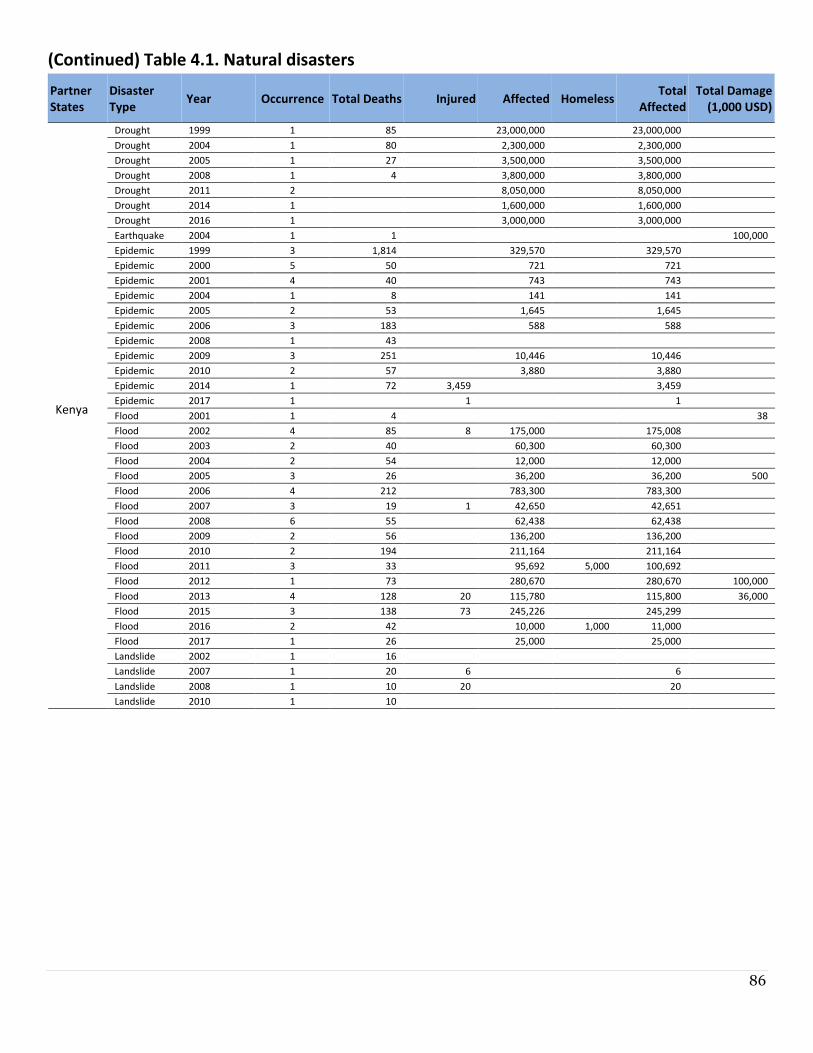
86
(Continued) Table 4.1. Natural disasters
Partner
States
Disaster
Type Year Occurrence Total Deaths Injured Affected Homeless
Total
Affected
Total Damage
(1,000 USD)
Kenya
Drought 1999 1 85 23,000,000 23,000,000
Drought 2004 1 80 2,300,000 2,300,000
Drought 2005 1 27 3,500,000 3,500,000
Drought 2008 1 4 3,800,000 3,800,000
Drought 2011 2 8,050,000 8,050,000
Drought 2014 1 1,600,000 1,600,000
Drought 2016 1 3,000,000 3,000,000
Earthquake 2004 1 1 100,000
Epidemic 1999 3 1,814 329,570 329,570
Epidemic 2000 5 50 721 721
Epidemic 2001 4 40 743 743
Epidemic 2004 1 8 141 141
Epidemic 2005 2 53 1,645 1,645
Epidemic 2006 3 183 588 588
Epidemic 2008 1 43
Epidemic 2009 3 251 10,446 10,446
Epidemic 2010 2 57 3,880 3,880
Epidemic 2014 1 72 3,459 3,459
Epidemic 2017 1 1 1
Flood 2001 1 4 38
Flood 2002 4 85 8 175,000 175,008
Flood 2003 2 40 60,300 60,300
Flood 2004 2 54 12,000 12,000
Flood 2005 3 26 36,200 36,200 500
Flood 2006 4 212 783,300 783,300
Flood 2007 3 19 1 42,650 42,651
Flood 2008 6 55 62,438 62,438
Flood 2009 2 56 136,200 136,200
Flood 2010 2 194 211,164 211,164
Flood 2011 3 33 95,692 5,000 100,692
Flood 2012 1 73 280,670 280,670 100,000
Flood 2013 4 128 20 115,780 115,800 36,000
Flood 2015 3 138 73 245,226 245,299
Flood 2016 2 42 10,000 1,000 11,000
Flood 2017 1 26 25,000 25,000
Landslide 2002 1 16
Landslide 2007 1 20 6 6
Landslide 2008 1 10 20 20
Landslide 2010 1 10
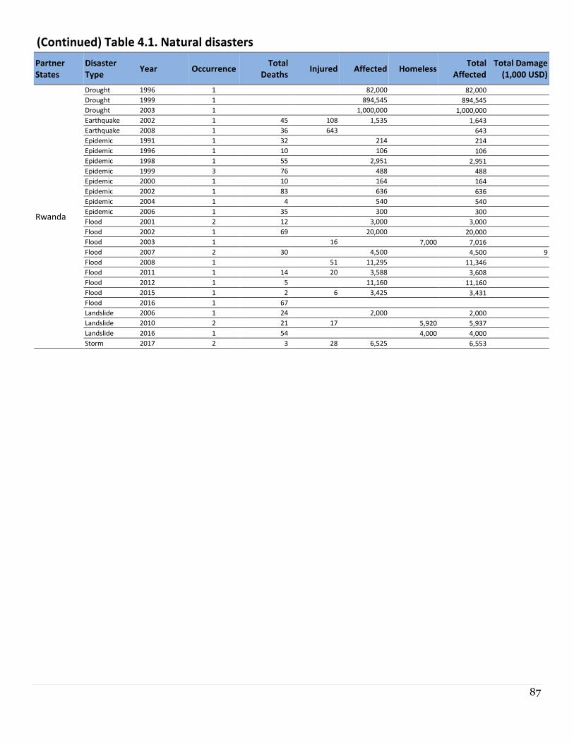
87
(Continued) Table 4.1. Natural disasters
Partner
States
Disaster
Type Year Occurrence
Total
Deaths Injured Affected Homeless
Total
Affected
Total Damage
(1,000 USD)
Rwanda
Drought 1996 1 82,000 82,000 Drought 1999 1 894,545 894,545 Drought 2003 1 1,000,000 1,000,000 Earthquake 2002 1 45 108 1,535 1,643 Earthquake 2008 1 36 643
643 Epidemic 1991 1 32 214 214 Epidemic 1996 1 10 106 106 Epidemic 1998 1 55 2,951 2,951 Epidemic 1999 3 76 488 488 Epidemic 2000 1 10 164 164 Epidemic 2002 1 83 636 636 Epidemic 2004 1 4 540 540 Epidemic 2006 1 35 300 300 Flood 2001 2 12 3,000 3,000 Flood 2002 1 69 20,000 20,000 Flood 2003 1 16 7,000 7,016 Flood 2007 2 30 4,500 4,500 9
Flood 2008 1 51 11,295 11,346 Flood 2011 1 14 20 3,588 3,608 Flood 2012 1 5 11,160 11,160 Flood 2015 1 2 6 3,425 3,431 Flood 2016 1 67 Landslide 2006 1 24 2,000 2,000 Landslide 2010 2 21 17 5,920 5,937 Landslide 2016 1 54 4,000 4,000 Storm 2017 2 3 28 6,525 6,553
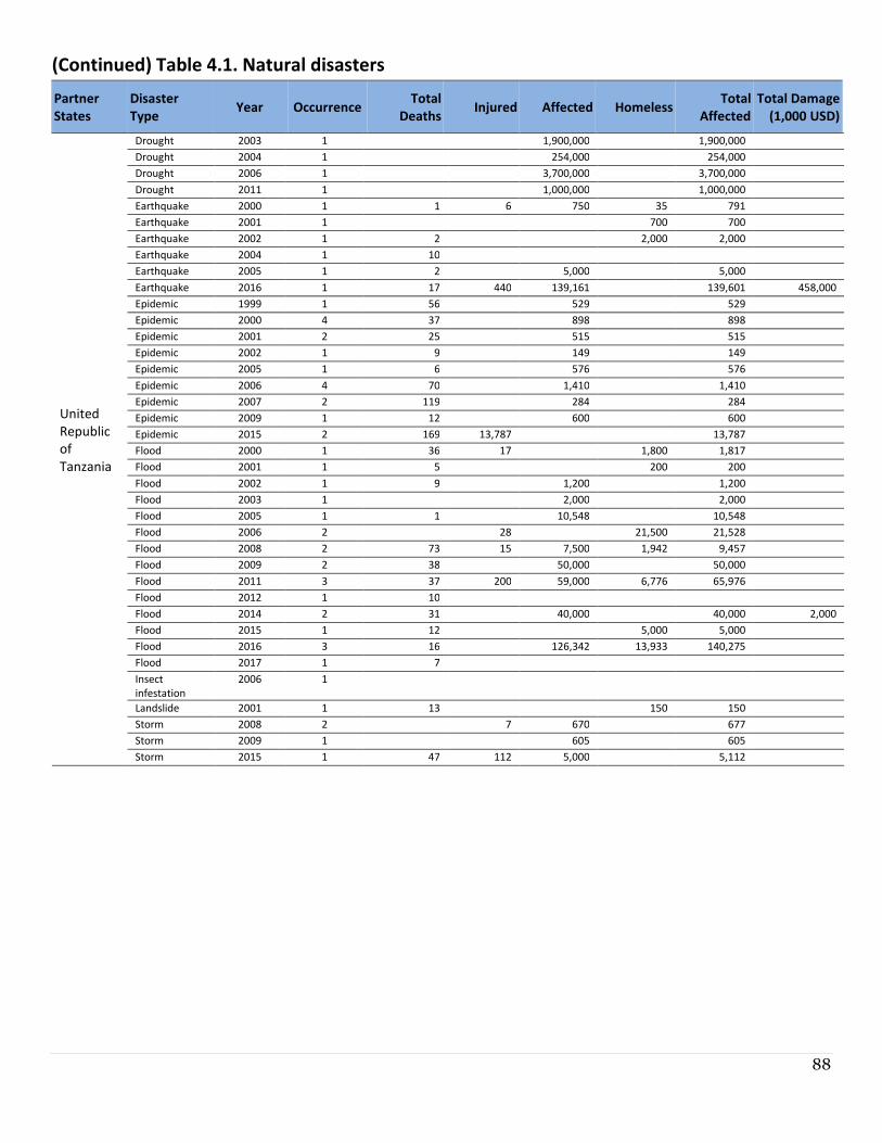
88
(Continued) Table 4.1. Natural disasters
Partner
States
Disaster
Type Year Occurrence
Total
Deaths Injured Affected Homeless
Total
Affected
Total Damage
(1,000 USD)
United
Republic
of
Tanzania
Drought 2003 1
1,900,000
1,900,000
Drought 2004 1
254,000
254,000
Drought 2006 1
3,700,000
3,700,000
Drought 2011 1
1,000,000
1,000,000
Earthquake 2000 1 1 6 750 35 791
Earthquake 2001 1
700 700
Earthquake 2002 1 2
2,000 2,000
Earthquake 2004 1 10
Earthquake 2005 1 2
5,000
5,000
Earthquake 2016 1 17 440 139,161
139,601 458,000
Epidemic 1999 1 56
529
529
Epidemic 2000 4 37
898
898
Epidemic 2001 2 25
515
515
Epidemic 2002 1 9
149
149
Epidemic 2005 1 6
576
576
Epidemic 2006 4 70
1,410
1,410
Epidemic 2007 2 119
284
284
Epidemic 2009 1 12
600
600
Epidemic 2015 2 169 13,787
13,787
Flood 2000 1 36 17
1,800 1,817
Flood 2001 1 5
200 200
Flood 2002 1 9
1,200
1,200
Flood 2003 1
2,000
2,000
Flood 2005 1 1
10,548
10,548
Flood 2006 2
28
21,500 21,528
Flood 2008 2 73 15 7,500 1,942 9,457
Flood 2009 2 38
50,000
50,000
Flood 2011 3 37 200 59,000 6,776 65,976
Flood 2012 1 10
Flood 2014 2 31
40,000
40,000 2,000
Flood 2015 1 12
5,000 5,000
Flood 2016 3 16
126,342 13,933 140,275
Flood 2017 1 7
Insect
infestation
2006 1
Landslide 2001 1 13
150 150
Storm 2008 2
7 670
677
Storm 2009 1
605
605
Storm 2015 1 47 112 5,000
5,112
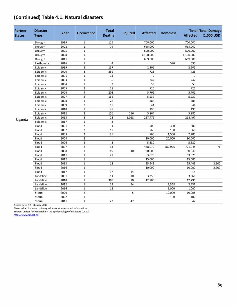
89
(Continued) Table 4.1. Natural disasters
Partner
States
Disaster
Type Year Occurrence
Total
Deaths Injured Affected Homeless
Total
Affected
Total Damage
(1,000 USD)
Uganda
Drought 1999 1 115
700,000
700,000
Drought 2002 1 79
655,000
655,000
Drought 2005 1
600,000
600,000
Drought 2008 1
1,100,000
1,100,000
Drought 2011 1
669,000
669,000
Earthquake 2016 1 4
590 590
Epidemic 1999 3 137
2,205
2,205
Epidemic 2000 3 259
723
723
Epidemic 2001 1 14
9
9
Epidemic 2003 1 35
242
242
Epidemic 2004 1 3
53
53
Epidemic 2005 2 21
726
726
Epidemic 2006 4 203
5,702
5,702
Epidemic 2007 2 132
5,937
5,937
Epidemic 2008 1 28
388
388
Epidemic 2009 2 17
544
544
Epidemic 2010 1 48
190
190
Epidemic 2012 3 156 116 5,864
5,980
Epidemic 2013 3 28 1,018 217,479
218,497
Epidemic 2017 1 3
Flood 2001 2 1
500 300 800
Flood 2002 2 17
760 100 860
Flood 2003 2 25
700 1,500 2,200
Flood 2004 2
10,000 20,000 30,000
Flood 2006 2 3
5,680
5,680
Flood 2007 2 33
438,070 282,975 721,045 71
Flood 2008 1 49 40 30,000
30,040
Flood 2011 1 27
63,075
63,075
Flood 2012 1
15,000
15,000
Flood 2013 1 13
25,445
25,445 3,100
Flood 2016 1
10,000
10,000 2,700
Flood 2017 1 17 14
14
Landslide 2001 1 11 10 3,356
3,366
Landslide 2010 1 388 10 12,785
12,795
Landslide 2012 1 18 64
3,368 3,432
Landslide 2016 1 15
1,000 1,000
Storm 2000 2
5
10,000 10,005
Storm 2002 1
100 100
Storm 2011 1 23 47
47
Access date: 12 February 2018
Blank values indicated missing values or non-reported information.
Source: Center for Research on the Epidemiology of Disasters (CRED)
http://www.emdat.be/
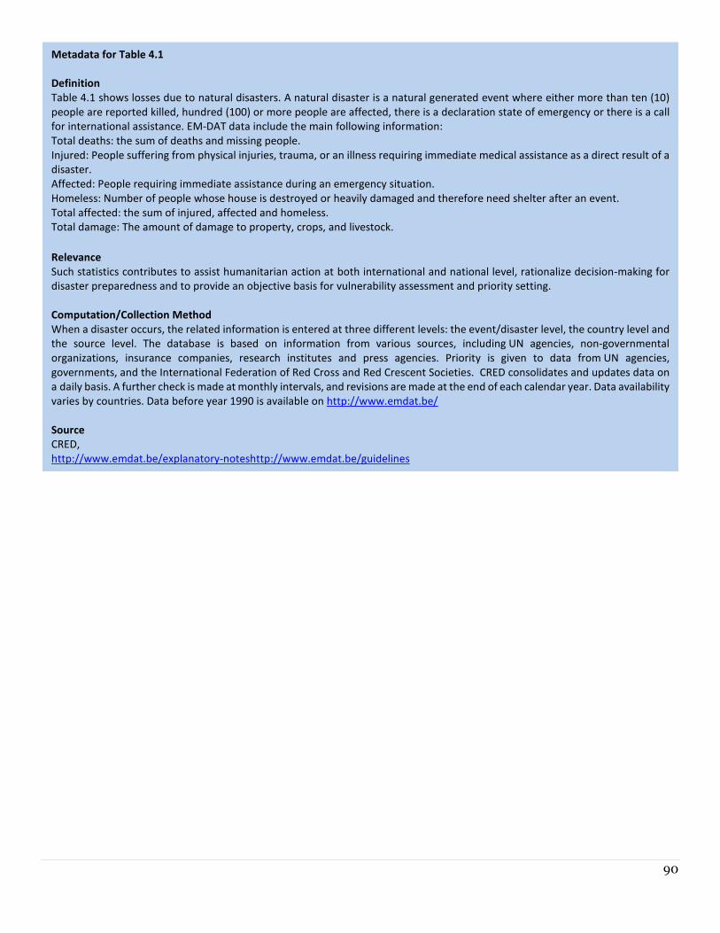
90
Metadata for Table 4.1
Definition
Table 4.1 shows losses due to natural disasters. A natural disaster is a natural generated event where either more than ten (10)
people are reported killed, hundred (100) or more people are affected, there is a declaration state of emergency or there is a call
for international assistance. EM-DAT data include the main following information:
Total deaths: the sum of deaths and missing people.
Injured: People suffering from physical injuries, trauma, or an illness requiring immediate medical assistance as a direct result of a
disaster.
Affected: People requiring immediate assistance during an emergency situation.
Homeless: Number of people whose house is destroyed or heavily damaged and therefore need shelter after an event.
Total affected: the sum of injured, affected and homeless.
Total damage: The amount of damage to property, crops, and livestock.
Relevance
Such statistics contributes to assist humanitarian action at both international and national level, rationalize decision-making for
disaster preparedness and to provide an objective basis for vulnerability assessment and priority setting.
Computation/Collection Method
When a disaster occurs, the related information is entered at three different levels: the event/disaster level, the country level and
the source level. The database is based on information from various sources, including UN agencies, non-governmental
organizations, insurance companies, research institutes and press agencies. Priority is given to data from UN agencies,
governments, and the International Federation of Red Cross and Red Crescent Societies. CRED consolidates and updates data on
a daily basis. A further check is made at monthly intervals, and revisions are made at the end of each calendar year. Data availability
varies by countries. Data before year 1990 is available on http://www.emdat.be/
Source
CRED,
http://www.emdat.be/explanatory-noteshttp://www.emdat.be/guidelines
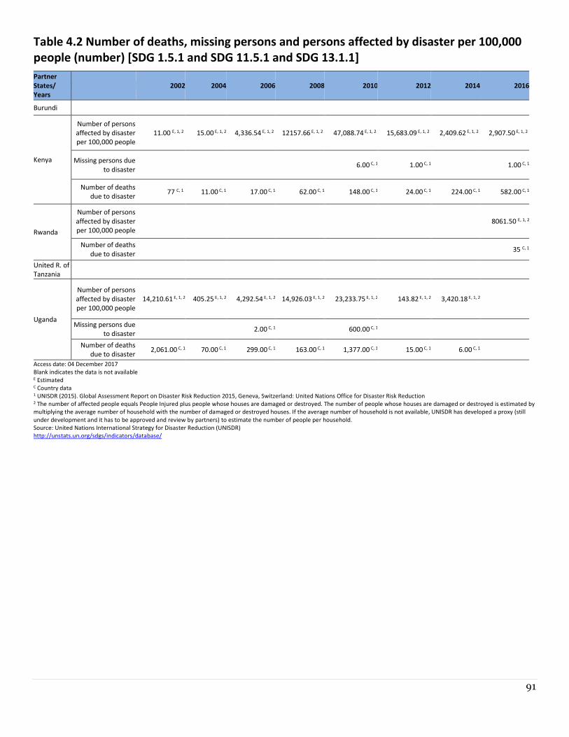
91
Table 4.2 Number of deaths, missing persons and persons affected by disaster per 100,000
people (number) [SDG 1.5.1 and SDG 11.5.1 and SDG 13.1.1]
Partner
States/
Years
2002 2004 2006 2008 2010 2012 2014 2016
Burundi
Kenya
Number of persons
affected by disaster
per 100,000 people
11.00 E, 1, 2 15.00 E, 1, 2 4,336.54 E, 1, 2 12157.66 E, 1, 2 47,088.74 E, 1, 2 15,683.09 E, 1, 2 2,409.62 E, 1, 2 2,907.50 E, 1, 2
Missing persons due
to disaster 6.00 C, 1 1.00 C, 1 1.00 C, 1
Number of deaths
due to disaster 77 C, 1 11.00 C, 1 17.00 C, 1 62.00 C, 1 148.00 C, 1 24.00 C, 1 224.00 C, 1 582.00 C, 1
Rwanda
Number of persons
affected by disaster
per 100,000 people
8061.50 E, 1, 2
Number of deaths
due to disaster 35 C, 1
United R. of
Tanzania
Uganda
Number of persons
affected by disaster
per 100,000 people
14,210.61 E, 1, 2 405.25 E, 1, 2 4,292.54 E, 1, 2 14,926.03 E, 1, 2 23,233.75 E, 1, 2 143.82 E, 1, 2 3,420.18 E, 1, 2
Missing persons due
to disaster 2.00 C, 1 600.00 C, 1
Number of deaths
due to disaster 2,061.00 C, 1 70.00 C, 1 299.00 C, 1 163.00 C, 1 1,377.00 C, 1 15.00 C, 1 6.00 C, 1
Access date: 04 December 2017
Blank indicates the data is not available E Estimated C Country data 1 UNISDR (2015). Global Assessment Report on Disaster Risk Reduction 2015, Geneva, Switzerland: United Nations Office for Disaster Risk Reduction 2 The number of affected people equals People Injured plus people whose houses are damaged or destroyed. The number of people whose houses are damaged or destroyed is estimated by
multiplying the average number of household with the number of damaged or destroyed houses. If the average number of household is not available, UNISDR has developed a proxy (still
under development and it has to be approved and review by partners) to estimate the number of people per household.
Source: United Nations International Strategy for Disaster Reduction (UNISDR)
http://unstats.un.org/sdgs/indicators/database/
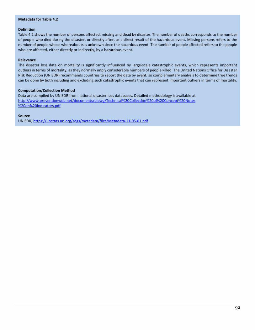
92
Metadata for Table 4.2
Definition
Table 4.2 shows the number of persons affected, missing and dead by disaster. The number of deaths corresponds to the number
of people who died during the disaster, or directly after, as a direct result of the hazardous event. Missing persons refers to the
number of people whose whereabouts is unknown since the hazardous event. The number of people affected refers to the people
who are affected, either directly or indirectly, by a hazardous event.
Relevance
The disaster loss data on mortality is significantly influenced by large-scale catastrophic events, which represents important
outliers in terms of mortality, as they normally imply considerable numbers of people killed. The United Nations Office for Disaster
Risk Reduction (UNISDR) recommends countries to report the data by event, so complementary analysis to determine true trends
can be done by both including and excluding such catastrophic events that can represent important outliers in terms of mortality.
Computation/Collection Method
Data are compiled by UNISDR from national disaster loss databases. Detailed methodology is available at
http://www.preventionweb.net/documents/oiewg/Technical%20Collection%20of%20Concept%20Notes
%20on%20Indicators.pdf.
Source
UNISDR, https://unstats.un.org/sdgs/metadata/files/Metadata-11-05-01.pdf
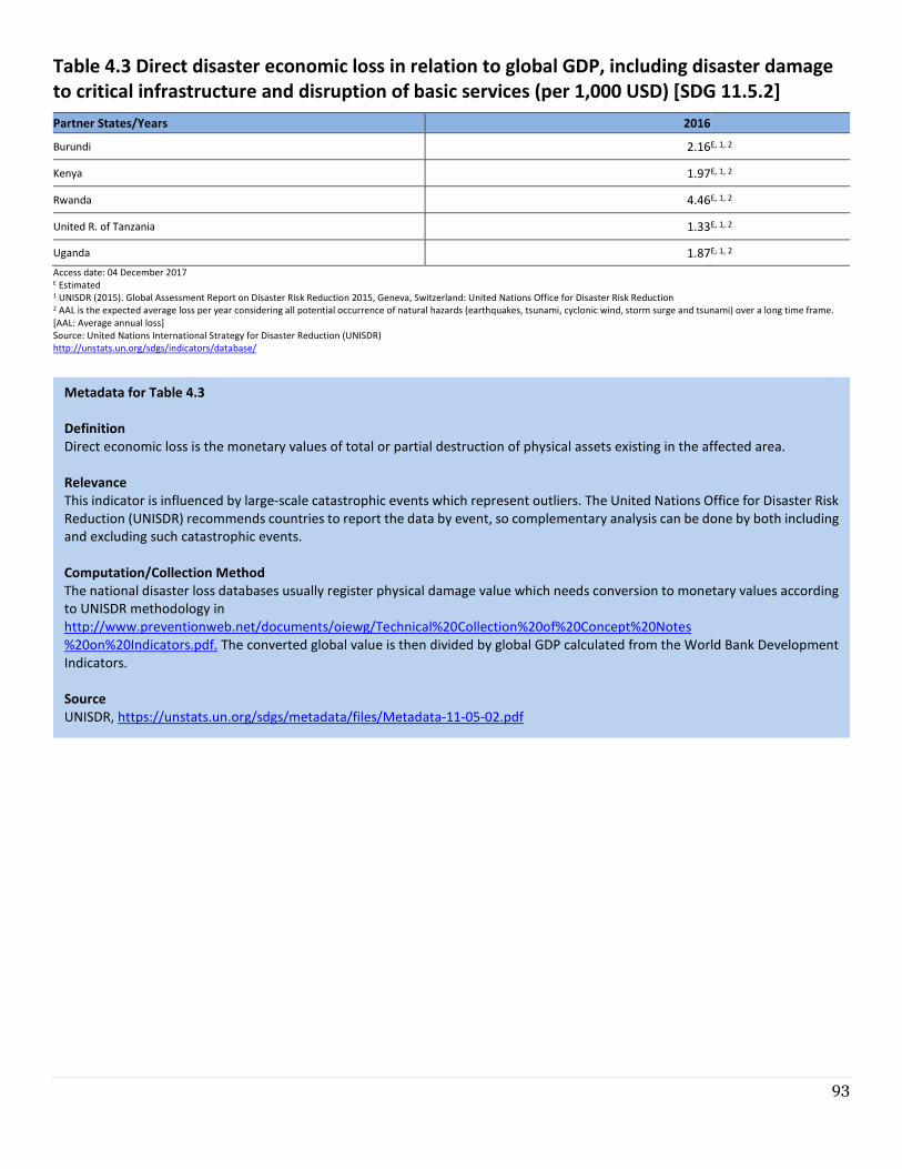
93
Table 4.3 Direct disaster economic loss in relation to global GDP, including disaster damage
to critical infrastructure and disruption of basic services (per 1,000 USD) [SDG 11.5.2]
Partner States/Years 2016
Burundi 2.16 E, 1, 2
Kenya 1.97E, 1, 2
Rwanda 4.46E, 1, 2
United R. of Tanzania 1.33E, 1, 2
Uganda 1.87E, 1, 2
Access date: 04 December 2017 E Estimated 1 UNISDR (2015). Global Assessment Report on Disaster Risk Reduction 2015, Geneva, Switzerland: United Nations Office for Disaster Risk Reduction 2 AAL is the expected average loss per year considering all potential occurrence of natural hazards (earthquakes, tsunami, cyclonic wind, storm surge and tsunami) over a long time frame.
[AAL: Average annual loss]
Source: United Nations International Strategy for Disaster Reduction (UNISDR)
http://unstats.un.org/sdgs/indicators/database/
Metadata for Table 4.3
Definition
Direct economic loss is the monetary values of total or partial destruction of physical assets existing in the affected area.
Relevance
This indicator is influenced by large-scale catastrophic events which represent outliers. The United Nations Office for Disaster Risk
Reduction (UNISDR) recommends countries to report the data by event, so complementary analysis can be done by both including
and excluding such catastrophic events.
Computation/Collection Method
The national disaster loss databases usually register physical damage value which needs conversion to monetary values according
to UNISDR methodology in
http://www.preventionweb.net/documents/oiewg/Technical%20Collection%20of%20Concept%20Notes
%20on%20Indicators.pdf. The converted global value is then divided by global GDP calculated from the World Bank Development
Indicators.
Source
UNISDR, https://unstats.un.org/sdgs/metadata/files/Metadata-11-05-02.pdf
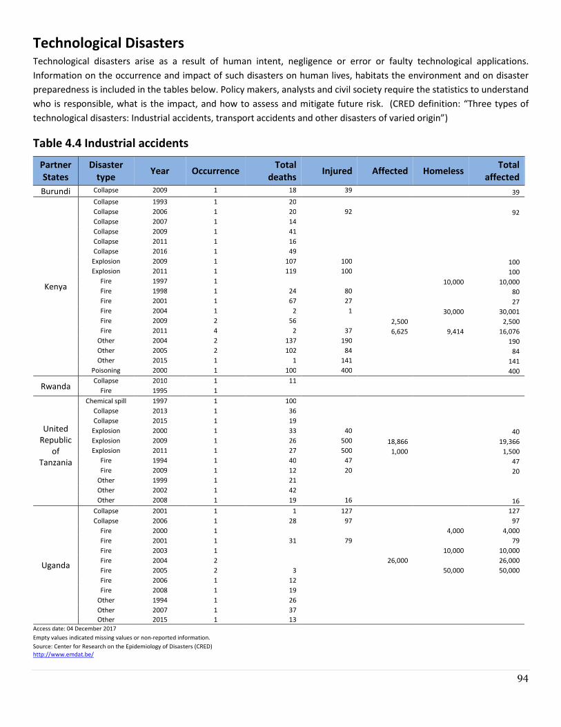
94
Technological Disasters Technological disasters arise as a result of human intent, negligence or error or faulty technological applications.
Information on the occurrence and impact of such disasters on human lives, habitats the environment and on disaster
preparedness is included in the tables below. Policy makers, analysts and civil society require the statistics to understand
who is responsible, what is the impact, and how to assess and mitigate future risk. (CRED definition: “Three types of
technological disasters: Industrial accidents, transport accidents and other disasters of varied origin”)
Table 4.4 Industrial accidents
Partner
States
Disaster
type Year Occurrence
Total
deaths Injured Affected Homeless
Total
affected
Burundi Collapse 2009 1 18 39 39
Kenya
Collapse 1993 1 20
Collapse 2006 1 20 92 92
Collapse 2007 1 14
Collapse 2009 1 41 Collapse 2011 1 16
Collapse 2016 1 49 Explosion 2009 1 107 100 100
Explosion 2011 1 119 100 100
Fire 1997 1
10,000 10,000
Fire 1998 1 24 80 80
Fire 2001 1 67 27 27
Fire 2004 1 2 1 30,000 30,001
Fire 2009 2 56
2,500 2,500
Fire 2011 4 2 37 6,625 9,414 16,076
Other 2004 2 137 190 190
Other 2005 2 102 84 84
Other 2015 1 1 141 141
Poisoning 2000 1 100 400 400
Rwanda Collapse 2010 1 11
Fire 1995 1
United
Republic
of
Tanzania
Chemical spill 1997 1 100
Collapse 2013 1 36 Collapse 2015 1 19
Explosion 2000 1 33 40 40
Explosion 2009 1 26 500 18,866 19,366
Explosion 2011 1 27 500 1,000 1,500
Fire 1994 1 40 47 47
Fire 2009 1 12 20 20
Other 1999 1 21
Other 2002 1 42 Other 2008 1 19 16 16
Uganda
Collapse 2001 1 1 127 127
Collapse 2006 1 28 97 97
Fire 2000 1 4,000 4,000
Fire 2001 1 31 79 79
Fire 2003 1 10,000 10,000
Fire 2004 2 26,000 26,000
Fire 2005 2 3 50,000 50,000
Fire 2006 1 12
Fire 2008 1 19
Other 1994 1 26
Other 2007 1 37
Other 2015 1 13
Access date: 04 December 2017
Empty values indicated missing values or non-reported information.
Source: Center for Research on the Epidemiology of Disasters (CRED)
http://www.emdat.be/
95
Metadata for Table 4.4
Definition
Table 4.4 shows losses due to technological disasters. Technological disasters are divided into 3 sub-groups among which industrial
accidents is one of them. EM-DAT data include the main following information:
Total deaths: the sum of deaths and missing people.
Injured: People suffering from physical injuries, trauma, or an illness requiring immediate medical assistance as a direct result of a
disaster.
Affected: People requiring immediate assistance during an emergency situation.
Homeless: Number of people whose house is destroyed or heavily damaged and therefore need shelter after an event.
Total affected: The total affected is the sum of injured, affected and homeless.
Relevance
Such statistics contributes to assist humanitarian action at both international and national level, rationalize decision-making for
disaster preparedness and to provide an objective basis for vulnerability assessment and priority setting.
Computation/Collection Method
When a disaster occurs, the related information is entered at three different levels: the event/disaster level, the country level and
the source level. The database is based on information from various sources, including UN agencies, non-governmental
organizations, insurance companies, research institutes and press agencies. Priority is given to data from UN agencies,
governments, and the International Federation of Red Cross and Red Crescent Societies. CRED consolidates and updates data on
a daily basis. A further check is made at monthly intervals, and revisions are made at the end of each calendar year.
Source
CRED,
http://www.emdat.be/explanatory-notes
http://www.emdat.be/guidelines
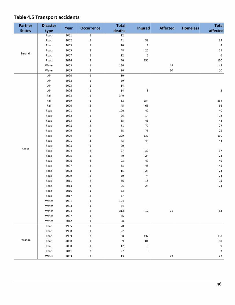
96
Table 4.5 Transport accidents
Partner
States
Disaster
type Year Occurrence
Total
deaths Injured Affected Homeless
Total
affected
Burundi
Road 2001 1 12
Road 2002 1 41 39
39
Road 2003 1 10 8 8
Road 2005 2 48 25
25
Road 2007 1 12 6 6
Road 2016 2 40 150
150
Water 2003 1 150 48 48
Water 2009 2 26
10
10
Kenya
Air 1990 1 10
Air 1992 1 50
Air 2003 1 14
Air 2006 1 14 3
3
Rail 1993 1 340
Rail 1999 1 32 254
254
Rail 2000 2 45 66 66
Road 1991 4 120 40
40
Road 1992 1 96 14 14
Road 1993 1 35 43
43
Road 1998 2 81 77 77
Road 1999 3 35 75
75
Road 2000 5 209 130 130
Road 2001 3 73 44
44
Road 2003 1 20
Road 2004 2 27 37
37
Road 2005 2 40 24 24
Road 2006 6 93 49
49
Road 2007 4 53 45 45
Road 2008 1 15 24
24
Road 2009 2 50 74 74
Road 2011 2 36 15
15
Road 2013 4 95 24 24
Road 2016 1 33
Road 2017 2 37
Water 1991 1 174
Water 1993 1 54
Water 1994 2 312 12 71
83
Water 1997 1 36
Water 2012 1 28
Rwanda
Road 1995 1 70
Road 1998 1 22
Road 1999 2 68 137 137
Road 2000 1 39 81
81
Road 2008 1 12 9 9
Road 2011 2 27 3
3
Water 2003 1 13 23 23
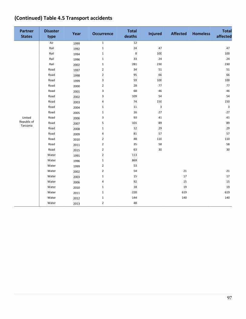
97
(Continued) Table 4.5 Transport accidents
Partner
States
Disaster
type Year Occurrence
Total
deaths Injured Affected Homeless
Total
affected
United
Republic of
Tanzania
Air 1999 1 12
Rail 1992 1 24 47 47
Rail 1994 1 8 100
100
Rail 1996 1 33 24 24
Rail 2002 1 281 230
230
Road 1997 2 34 51 51
Road 1998 2 95 66
66
Road 1999 3 59 100 100
Road 2000 2 28 77
77
Road 2001 3 68 46 46
Road 2002 3 109 54
54
Road 2003 4 74 150 150
Road 2004 1 11 3
3
Road 2005 1 16 27 27
Road 2006 3 93 41
41
Road 2007 5 101 89 89
Road 2008 1 12 29
29
Road 2009 4 81 57 57
Road 2010 2 48 110
110
Road 2011 2 35 58 58
Road 2015 2 63 30
30
Water 1991 2 113
Water 1996 1 869
Water 1999 2 53
Water 2002 2 54
21
21
Water 2003 1 15 17 17
Water 2006 4 92
15
15
Water 2010 1 18 19 19
Water 2011 1 220
619
619
Water 2012 1 144 140 140
Water 2013 2 48
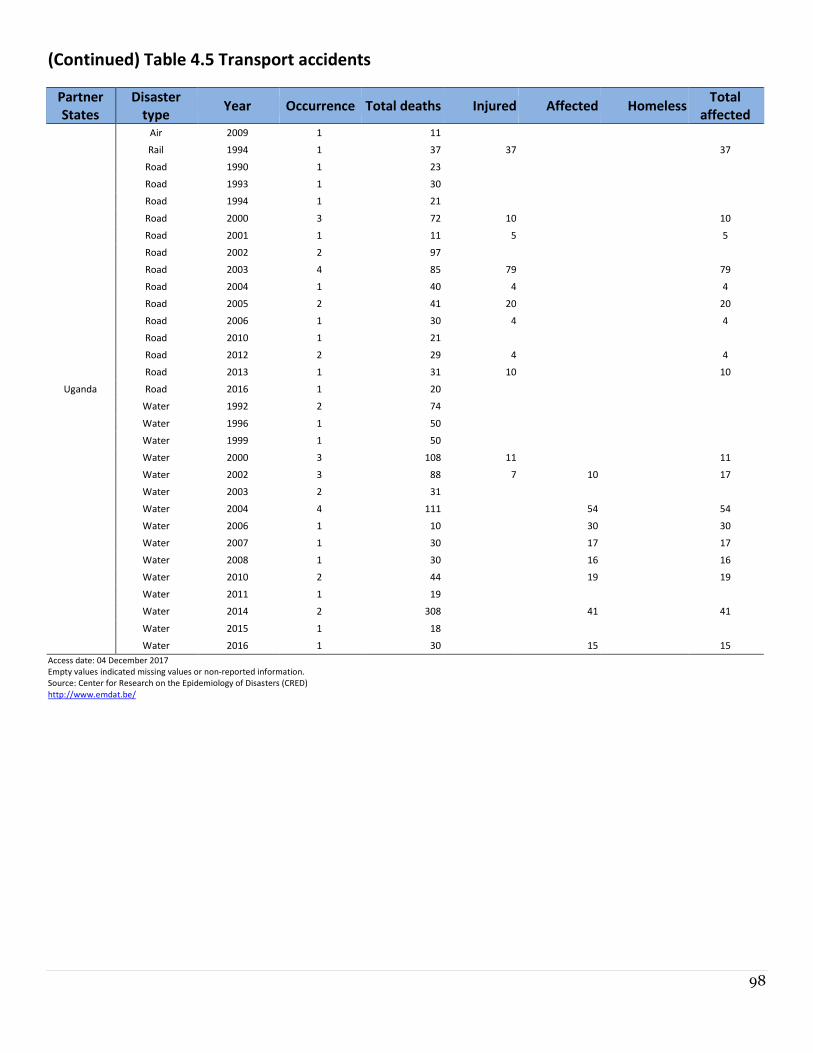
98
(Continued) Table 4.5 Transport accidents
Partner
States
Disaster
type Year Occurrence Total deaths Injured Affected Homeless
Total
affected
Uganda
Air 2009 1 11
Rail 1994 1 37 37 37
Road 1990 1 23
Road 1993 1 30
Road 1994 1 21
Road 2000 3 72 10 10
Road 2001 1 11 5 5
Road 2002 2 97
Road 2003 4 85 79 79
Road 2004 1 40 4 4
Road 2005 2 41 20 20
Road 2006 1 30 4 4
Road 2010 1 21
Road 2012 2 29 4 4
Road 2013 1 31 10 10
Road 2016 1 20
Water 1992 2 74
Water 1996 1 50
Water 1999 1 50
Water 2000 3 108 11 11
Water 2002 3 88 7 10 17
Water 2003 2 31
Water 2004 4 111 54 54
Water 2006 1 10 30 30
Water 2007 1 30 17 17
Water 2008 1 30 16 16
Water 2010 2 44 19 19
Water 2011 1 19
Water 2014 2 308 41 41
Water 2015 1 18
Water 2016 1 30 15 15
Access date: 04 December 2017
Empty values indicated missing values or non-reported information.
Source: Center for Research on the Epidemiology of Disasters (CRED)
http://www.emdat.be/
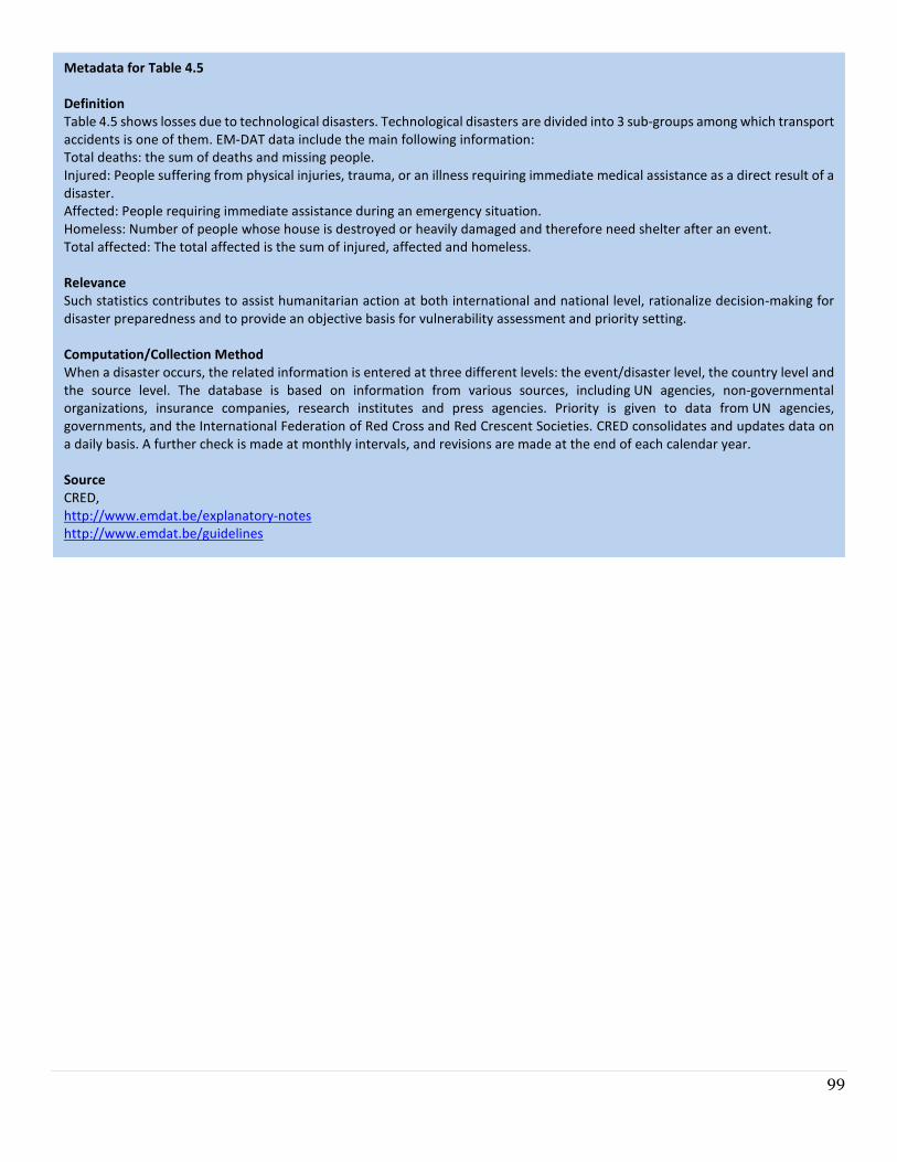
99
Metadata for Table 4.5
Definition
Table 4.5 shows losses due to technological disasters. Technological disasters are divided into 3 sub-groups among which transport
accidents is one of them. EM-DAT data include the main following information:
Total deaths: the sum of deaths and missing people.
Injured: People suffering from physical injuries, trauma, or an illness requiring immediate medical assistance as a direct result of a
disaster.
Affected: People requiring immediate assistance during an emergency situation.
Homeless: Number of people whose house is destroyed or heavily damaged and therefore need shelter after an event.
Total affected: The total affected is the sum of injured, affected and homeless.
Relevance
Such statistics contributes to assist humanitarian action at both international and national level, rationalize decision-making for
disaster preparedness and to provide an objective basis for vulnerability assessment and priority setting.
Computation/Collection Method
When a disaster occurs, the related information is entered at three different levels: the event/disaster level, the country level and
the source level. The database is based on information from various sources, including UN agencies, non-governmental
organizations, insurance companies, research institutes and press agencies. Priority is given to data from UN agencies,
governments, and the International Federation of Red Cross and Red Crescent Societies. CRED consolidates and updates data on
a daily basis. A further check is made at monthly intervals, and revisions are made at the end of each calendar year.
Source
CRED,
http://www.emdat.be/explanatory-notes
http://www.emdat.be/guidelines
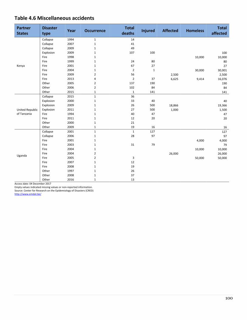
100
Table 4.6 Miscellaneous accidents
Partner
States
Disaster
type Year Occurrence
Total
deaths Injured Affected Homeless
Total
affected
Kenya
Collapse 1994 1 14
Collapse 2007 1 41
Collapse 2009 1 49
Explosion 2009 1 107 100 100
Fire 1998 1 10,000 10,000
Fire 1999 1 24 80 80
Fire 2001 1 67 27 27
Fire 2004 1 2 1 30,000 30,001
Fire 2009 2 56 2,500 2,500
Fire 2013 4 2 37 6,625 9,414 16,076
Other 2005 2 137 190 190
Other 2006 2 102 84 84
Other 2015 1 1 141 141
United Republic
of Tanzania
Collapse 2015 1 36
Explosion 2000 1 33 40 40
Explosion 2009 1 26 500 18,866 19,366
Explosion 2011 1 27 500 1,000 1,500
Fire 1994 1 40 47 47
Fire 2011 1 12 20 20
Other 2000 1 21
Other 2009 1 19 16 16
Uganda
Collapse 2001 1 1 127 127
Collapse 2006 1 28 97 97
Fire 2001 1 4,000 4,000
Fire 2003 1 31 79 79
Fire 2004 1 10,000 10,000
Fire 2004 2 26,000 26,000
Fire 2005 2 3 50,000 50,000
Fire 2007 1 12
Fire 2008 1 19
Other 1997 1 26
Other 2008 1 37
Other 2016 1 13
Access date: 04 December 2017
Empty values indicated missing values or non-reported information.
Source: Center for Research on the Epidemiology of Disasters (CRED)
http://www.emdat.be/
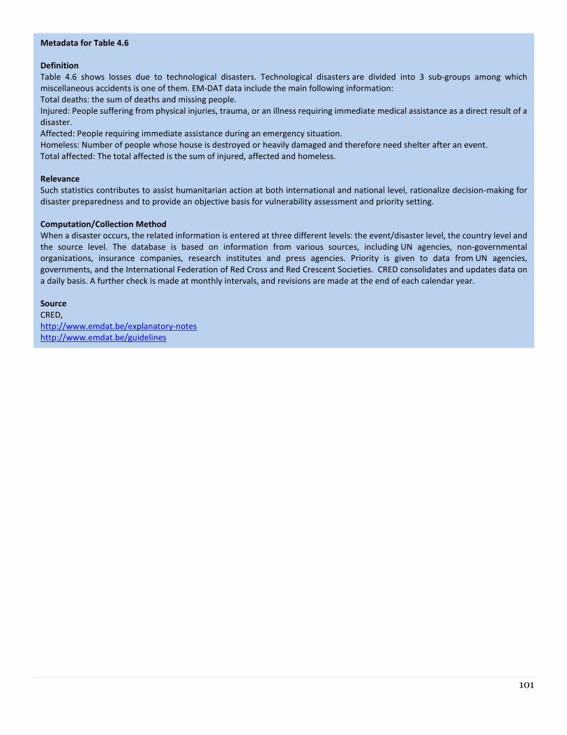
101
Metadata for Table 4.6
Definition
Table 4.6 shows losses due to technological disasters. Technological disasters are divided into 3 sub-groups among which
miscellaneous accidents is one of them. EM-DAT data include the main following information:
Total deaths: the sum of deaths and missing people.
Injured: People suffering from physical injuries, trauma, or an illness requiring immediate medical assistance as a direct result of a
disaster.
Affected: People requiring immediate assistance during an emergency situation.
Homeless: Number of people whose house is destroyed or heavily damaged and therefore need shelter after an event.
Total affected: The total affected is the sum of injured, affected and homeless.
Relevance
Such statistics contributes to assist humanitarian action at both international and national level, rationalize decision-making for
disaster preparedness and to provide an objective basis for vulnerability assessment and priority setting.
Computation/Collection Method
When a disaster occurs, the related information is entered at three different levels: the event/disaster level, the country level and
the source level. The database is based on information from various sources, including UN agencies, non-governmental
organizations, insurance companies, research institutes and press agencies. Priority is given to data from UN agencies,
governments, and the International Federation of Red Cross and Red Crescent Societies. CRED consolidates and updates data on
a daily basis. A further check is made at monthly intervals, and revisions are made at the end of each calendar year.
Source
CRED,
http://www.emdat.be/explanatory-notes
http://www.emdat.be/guidelines
102
Chapter 5 Human Settlements and
Environmental Health
103
CHAPTER 5 HUMAN SETTLEMENTS AND ENVIRONMENTAL
HEALTH
This chapter encompasses statistics on the environment in which humans live and work, particularly with regard to living
conditions and environmental health. These statistics are important for the management and improvement of conditions
related to human settlements, shelter conditions, safe water, sanitation and health. Increasing concentration of humans
in modern urban settlements pose special challenges to humans and their physical environment in which these
settlements are located. The well-being and health risks associated with the environment can be mitigated substantially
by the prevailing conditions and characteristics of human settlements. Appropriate infrastructure, adequate waste
disposal, wise land use planning, clean and safe transportation and ecosystem health, among others, can modify the effect
of environmental and settlement-related risks on human well-being.
Human Settlements Statistics on basic services and infrastructure of human settlements, access to selected basic services, housing conditions,
and exposure to ambient pollution, are included below. Policy makers, analysts and civil society need these statistics for
information on how humans live and work in these settlements, how they transform the landscape and the supporting
ecosystem and how this affects human well-being and health. Data sources include censuses, surveys, administrative
records and remote sensors.
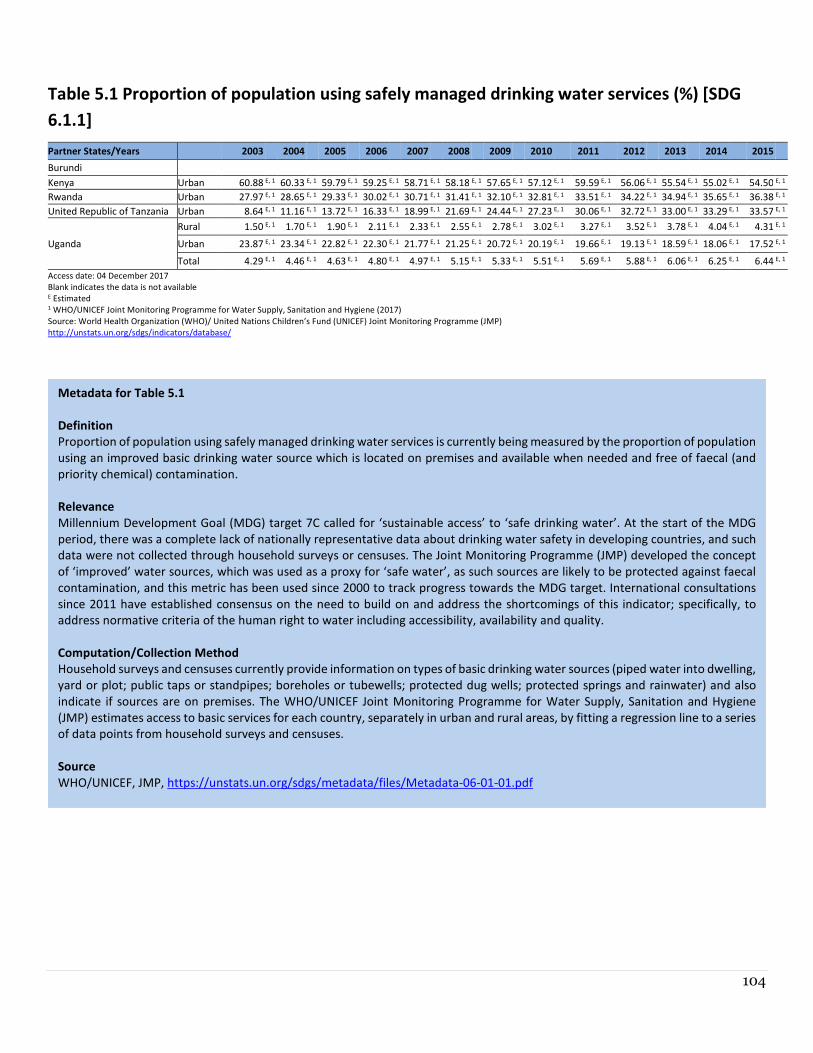
104
Table 5.1 Proportion of population using safely managed drinking water services (%) [SDG
6.1.1]
Partner States/Years 2003 2004 2005 2006 2007 2008 2009 2010 2011 2012 2013 2014 2015
Burundi
Kenya Urban 60.88 E, 1 60.33 E, 1 59.79 E, 1 59.25 E, 1 58.71 E, 1 58.18 E, 1 57.65 E, 1 57.12 E, 1 59.59 E, 1 56.06 E, 1 55.54 E, 1 55.02 E, 1 54.50 E, 1
Rwanda Urban 27.97 E, 1 28.65 E, 1 29.33 E, 1 30.02 E, 1 30.71 E, 1 31.41 E, 1 32.10 E, 1 32.81 E, 1 33.51 E, 1 34.22 E, 1 34.94 E, 1 35.65 E, 1 36.38 E, 1
United Republic of Tanzania Urban 8.64 E, 1 11.16 E, 1 13.72 E, 1 16.33 E, 1 18.99 E, 1 21.69 E, 1 24.44 E, 1 27.23 E, 1 30.06 E, 1 32.72 E, 1 33.00 E, 1 33.29 E, 1 33.57 E, 1
Uganda
Rural 1.50 E, 1 1.70 E, 1 1.90 E, 1 2.11 E, 1 2.33 E, 1 2.55 E, 1 2.78 E, 1 3.02 E, 1 3.27 E, 1 3.52 E, 1 3.78 E, 1 4.04 E, 1 4.31 E, 1
Urban 23.87 E, 1 23.34 E, 1 22.82 E, 1 22.30 E, 1 21.77 E, 1 21.25 E, 1 20.72 E, 1 20.19 E, 1 19.66 E, 1 19.13 E, 1 18.59 E, 1 18.06 E, 1 17.52 E, 1
Total 4.29 E, 1 4.46 E, 1 4.63 E, 1 4.80 E, 1 4.97 E, 1 5.15 E, 1 5.33 E, 1 5.51 E, 1 5.69 E, 1 5.88 E, 1 6.06 E, 1 6.25 E, 1 6.44 E, 1
Access date: 04 December 2017
Blank indicates the data is not available E Estimated 1 WHO/UNICEF Joint Monitoring Programme for Water Supply, Sanitation and Hygiene (2017)
Source: World Health Organization (WHO)/ United Nations Children’s Fund (UNICEF) Joint Monitoring Programme (JMP)
http://unstats.un.org/sdgs/indicators/database/
Metadata for Table 5.1
Definition
Proportion of population using safely managed drinking water services is currently being measured by the proportion of population
using an improved basic drinking water source which is located on premises and available when needed and free of faecal (and
priority chemical) contamination.
Relevance
Millennium Development Goal (MDG) target 7C called for ‘sustainable access’ to ‘safe drinking water’. At the start of the MDG
period, there was a complete lack of nationally representative data about drinking water safety in developing countries, and such
data were not collected through household surveys or censuses. The Joint Monitoring Programme (JMP) developed the concept
of ‘improved’ water sources, which was used as a proxy for ‘safe water’, as such sources are likely to be protected against faecal
contamination, and this metric has been used since 2000 to track progress towards the MDG target. International consultations
since 2011 have established consensus on the need to build on and address the shortcomings of this indicator; specifically, to
address normative criteria of the human right to water including accessibility, availability and quality.
Computation/Collection Method
Household surveys and censuses currently provide information on types of basic drinking water sources (piped water into dwelling,
yard or plot; public taps or standpipes; boreholes or tubewells; protected dug wells; protected springs and rainwater) and also
indicate if sources are on premises. The WHO/UNICEF Joint Monitoring Programme for Water Supply, Sanitation and Hygiene
(JMP) estimates access to basic services for each country, separately in urban and rural areas, by fitting a regression line to a series
of data points from household surveys and censuses.
Source
WHO/UNICEF, JMP, https://unstats.un.org/sdgs/metadata/files/Metadata-06-01-01.pdf
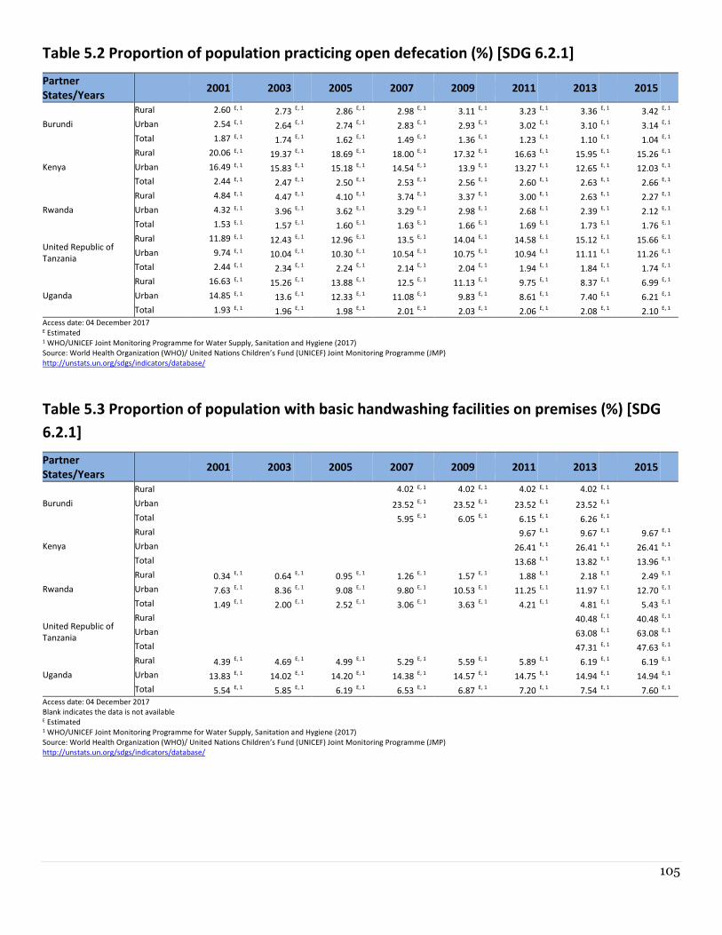
105
Table 5.2 Proportion of population practicing open defecation (%) [SDG 6.2.1]
Partner
States/Years 2001 2003 2005 2007 2009 2011 2013 2015
Burundi
Rural 2.60 E, 1 2.73
E, 1 2.86
E, 1 2.98
E, 1 3.11
E, 1 3.23
E, 1 3.36
E, 1 3.42
E, 1
Urban 2.54 E, 1 2.64
E, 1 2.74
E, 1 2.83
E, 1 2.93
E, 1 3.02
E, 1 3.10
E, 1 3.14
E, 1
Total 1.87 E, 1 1.74
E, 1 1.62
E, 1 1.49
E, 1 1.36
E, 1 1.23
E, 1 1.10
E, 1 1.04
E, 1
Kenya
Rural 20.06 E, 1 19.37
E, 1 18.69
E, 1 18.00
E, 1 17.32
E, 1 16.63
E, 1 15.95
E, 1 15.26
E, 1
Urban 16.49 E, 1 15.83 E, 1 15.18 E, 1 14.54 E, 1 13.9 E, 1 13.27 E, 1 12.65 E, 1 12.03 E, 1
Total 2.44 E, 1 2.47
E, 1 2.50
E, 1 2.53
E, 1 2.56
E, 1 2.60
E, 1 2.63
E, 1 2.66
E, 1
Rwanda
Rural 4.84 E, 1 4.47
E, 1 4.10
E, 1 3.74
E, 1 3.37
E, 1 3.00
E, 1 2.63
E, 1 2.27
E, 1
Urban 4.32 E, 1 3.96
E, 1 3.62
E, 1 3.29
E, 1 2.98
E, 1 2.68
E, 1 2.39
E, 1 2.12
E, 1
Total 1.53 E, 1 1.57
E, 1 1.60
E, 1 1.63
E, 1 1.66
E, 1 1.69
E, 1 1.73
E, 1 1.76
E, 1
United Republic of
Tanzania
Rural 11.89 E, 1 12.43
E, 1 12.96
E, 1 13.5
E, 1 14.04
E, 1 14.58
E, 1 15.12
E, 1 15.66
E, 1
Urban 9.74 E, 1 10.04 E, 1 10.30 E, 1 10.54 E, 1 10.75 E, 1 10.94 E, 1 11.11 E, 1 11.26 E, 1
Total 2.44 E, 1 2.34
E, 1 2.24
E, 1 2.14
E, 1 2.04
E, 1 1.94
E, 1 1.84
E, 1 1.74
E, 1
Uganda
Rural 16.63 E, 1 15.26
E, 1 13.88
E, 1 12.5
E, 1 11.13
E, 1 9.75
E, 1 8.37
E, 1 6.99
E, 1
Urban 14.85 E, 1 13.6
E, 1 12.33
E, 1 11.08
E, 1 9.83
E, 1 8.61
E, 1 7.40
E, 1 6.21
E, 1
Total 1.93 E, 1 1.96
E, 1 1.98
E, 1 2.01
E, 1 2.03
E, 1 2.06
E, 1 2.08
E, 1 2.10
E, 1
Access date: 04 December 2017 E Estimated 1 WHO/UNICEF Joint Monitoring Programme for Water Supply, Sanitation and Hygiene (2017)
Source: World Health Organization (WHO)/ United Nations Children’s Fund (UNICEF) Joint Monitoring Programme (JMP)
http://unstats.un.org/sdgs/indicators/database/
Table 5.3 Proportion of population with basic handwashing facilities on premises (%) [SDG
6.2.1]
Partner
States/Years 2001 2003 2005 2007 2009 2011 2013 2015
Burundi
Rural 4.02 E, 1 4.02 E, 1 4.02 E, 1 4.02 E, 1
Urban 23.52
E, 1 23.52
E, 1 23.52
E, 1 23.52
E, 1
Total 5.95
E, 1 6.05
E, 1 6.15
E, 1 6.26
E, 1
Kenya
Rural 9.67 E, 1 9.67 E, 1 9.67 E, 1
Urban 26.41
E, 1 26.41
E, 1 26.41
E, 1
Total 13.68
E, 1 13.82
E, 1 13.96
E, 1
Rwanda
Rural 0.34 E, 1
0.64 E, 1
0.95 E, 1
1.26 E, 1
1.57 E, 1
1.88 E, 1
2.18 E, 1
2.49 E, 1
Urban 7.63 E, 1
8.36 E, 1
9.08 E, 1
9.80 E, 1
10.53 E, 1
11.25 E, 1
11.97 E, 1
12.70 E, 1
Total 1.49 E, 1
2.00 E, 1
2.52 E, 1
3.06 E, 1
3.63 E, 1
4.21 E, 1
4.81 E, 1
5.43 E, 1
United Republic of
Tanzania
Rural 40.48 E, 1 40.48 E, 1
Urban 63.08
E, 1 63.08
E, 1
Total 47.31
E, 1 47.63
E, 1
Uganda
Rural 4.39 E, 1
4.69 E, 1
4.99 E, 1
5.29 E, 1
5.59 E, 1
5.89 E, 1
6.19 E, 1
6.19 E, 1
Urban 13.83 E, 1
14.02 E, 1
14.20 E, 1
14.38 E, 1
14.57 E, 1
14.75 E, 1
14.94 E, 1
14.94 E, 1
Total 5.54 E, 1
5.85 E, 1
6.19 E, 1
6.53 E, 1
6.87 E, 1
7.20 E, 1
7.54 E, 1
7.60 E, 1
Access date: 04 December 2017
Blank indicates the data is not available E Estimated 1 WHO/UNICEF Joint Monitoring Programme for Water Supply, Sanitation and Hygiene (2017)
Source: World Health Organization (WHO)/ United Nations Children’s Fund (UNICEF) Joint Monitoring Programme (JMP)
http://unstats.un.org/sdgs/indicators/database/
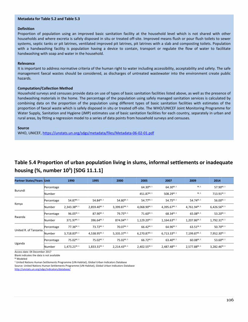
106
Table 5.4 Proportion of urban population living in slums, informal settlements or inadequate
housing (%, number 103) [SDG 11.1.1]
Partner States/Years Unit 1990 1995 2000 2005 2007 2009 2014
Burundi Percentage 64.30M, 1 64.30M, 1 M, 1 57.90M, 1
Number 451.87M, 1 508.29M, 1 M, 1 713.91M, 1
Kenya Percentage 54.87M, 1 54.84M, 1 54.80M, 1 54.77M, 1 54.75M, 1 54.74M, 1 56.00M, 1
Number 2,343.38M, 1 2,859.40M, 1 3,399.87M, 1 4,068.90M, 1 4,395.67M, 1 4,761.94M, 1 6,426.56M, 1
Rwanda Percentage 96.05M, 1 87.90M, 1 79.75M, 1 71.60M, 1 68.34M, 1 65.08M, 1 53.20M, 1
Number 371.97M, 1 396.64M, 1 874.04M, 1 1,129.20M, 1 1,164.63M, 1 1,207.86M, 1 1,792.31M, 1
United R. of Tanzania Percentage 77.36M, 1 73.72M, 1 70.07M, 1 66.42M, 1 64.96M, 1 63.51M, 1 50.70M, 1
Number 3,718.83M, 1 4,538.95M, 1 5,335.37M, 1 6,270.87M, 1 6,713.33M, 1 7,199.87M, 1 7,952.30M, 1
Uganda Percentage 75.02M, 1 75.02M, 1 75.02M, 1 66.72M, 1 63.40M, 1 60.08M, 1 53.60M, 1
Number 1,473.21M, 1 1,833.31M, 1 2,214.43M, 1 2,402.55M, 1 2,487.48M, 1 2,577.88M, 1 3,282.46M, 1
Access date: 04 December 2017
Blank indicates the data is not available M Modeled 1 United Nations Human Settlements Programme (UN-Habitat), Global Urban Indicators Database
Source: United Nations Human Settlements Programme (UN-Habitat), Global Urban Indicators Database
http://unstats.un.org/sdgs/indicators/database/
Metadata for Table 5.2 and Table 5.3
Definition
Proportion of population using an improved basic sanitation facility at the household level which is not shared with other
households and where excreta is safely disposed in situ or treated off-site. Improved means flush or pour flush toilets to sewer
systems, septic tanks or pit latrines, ventilated improved pit latrines, pit latrines with a slab and composting toilets. Population
with a handwashing facility is population having a device to contain, transport or regulate the flow of water to facilitate
handwashing with soap and water in the household.
Relevance
It is important to address normative criteria of the human right to water including accessibility, acceptability and safety. The safe
management faecal wastes should be considered, as discharges of untreated wastewater into the environment create public
hazards.
Computation/Collection Method
Household surveys and censuses provide data on use of types of basic sanitation facilities listed above, as well as the presence of
handwashing materials in the home. The percentage of the population using safely managed sanitation services is calculated by
combining data on the proportion of the population using different types of basic sanitation facilities with estimates of the
proportion of faecal waste which is safely disposed in situ or treated off-site. The WHO/UNICEF Joint Monitoring Programme for
Water Supply, Sanitation and Hygiene (JMP) estimates use of basic sanitation facilities for each country, separately in urban and
rural areas, by fitting a regression model to a series of data points from household surveys and censuses.
Source
WHO, UNICEF, https://unstats.un.org/sdgs/metadata/files/Metadata-06-02-01.pdf
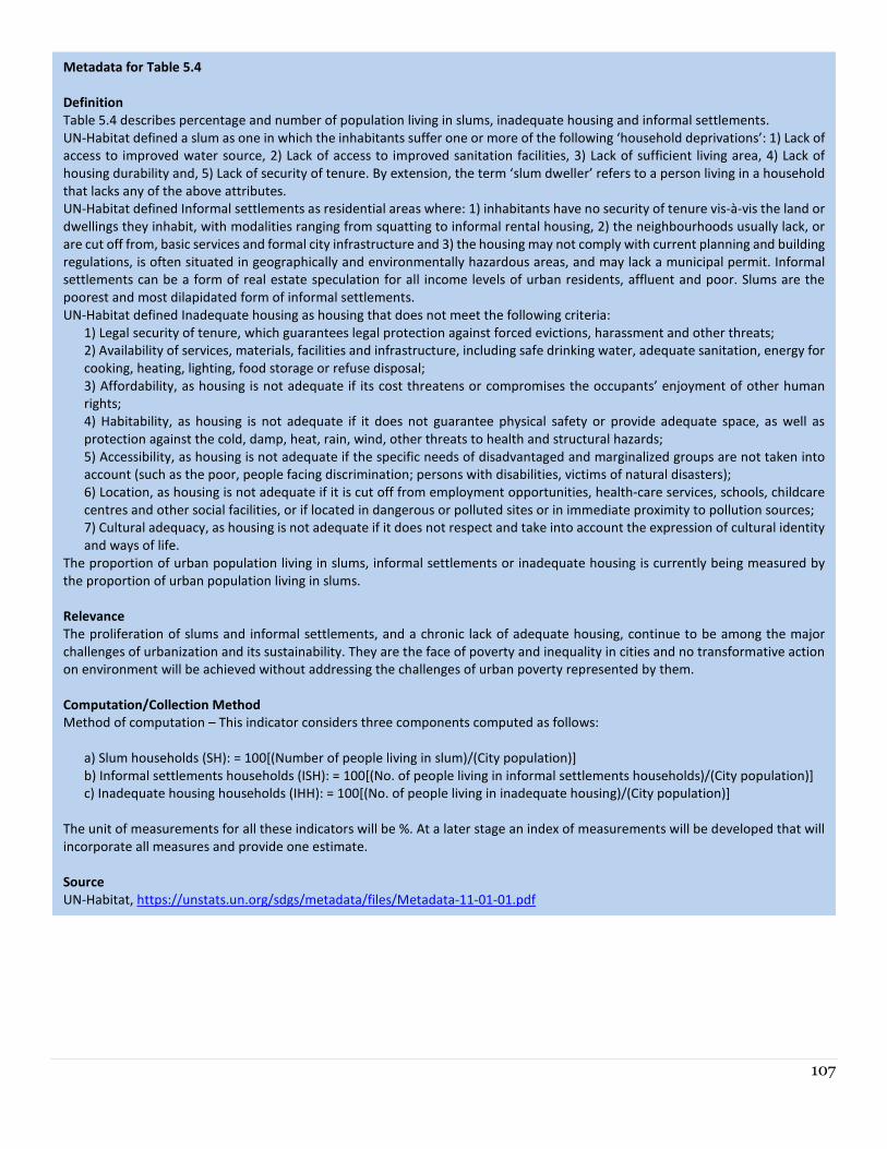
107
Metadata for Table 5.4
Definition
Table 5.4 describes percentage and number of population living in slums, inadequate housing and informal settlements.
UN-Habitat defined a slum as one in which the inhabitants suffer one or more of the following ‘household deprivations’: 1) Lack of
access to improved water source, 2) Lack of access to improved sanitation facilities, 3) Lack of sufficient living area, 4) Lack of
housing durability and, 5) Lack of security of tenure. By extension, the term ‘slum dweller’ refers to a person living in a household
that lacks any of the above attributes.
UN-Habitat defined Informal settlements as residential areas where: 1) inhabitants have no security of tenure vis-à-vis the land or
dwellings they inhabit, with modalities ranging from squatting to informal rental housing, 2) the neighbourhoods usually lack, or
are cut off from, basic services and formal city infrastructure and 3) the housing may not comply with current planning and building
regulations, is often situated in geographically and environmentally hazardous areas, and may lack a municipal permit. Informal
settlements can be a form of real estate speculation for all income levels of urban residents, affluent and poor. Slums are the
poorest and most dilapidated form of informal settlements.
UN-Habitat defined Inadequate housing as housing that does not meet the following criteria:
1) Legal security of tenure, which guarantees legal protection against forced evictions, harassment and other threats;
2) Availability of services, materials, facilities and infrastructure, including safe drinking water, adequate sanitation, energy for
cooking, heating, lighting, food storage or refuse disposal;
3) Affordability, as housing is not adequate if its cost threatens or compromises the occupants’ enjoyment of other human
rights;
4) Habitability, as housing is not adequate if it does not guarantee physical safety or provide adequate space, as well as
protection against the cold, damp, heat, rain, wind, other threats to health and structural hazards;
5) Accessibility, as housing is not adequate if the specific needs of disadvantaged and marginalized groups are not taken into
account (such as the poor, people facing discrimination; persons with disabilities, victims of natural disasters);
6) Location, as housing is not adequate if it is cut off from employment opportunities, health-care services, schools, childcare
centres and other social facilities, or if located in dangerous or polluted sites or in immediate proximity to pollution sources;
7) Cultural adequacy, as housing is not adequate if it does not respect and take into account the expression of cultural identity
and ways of life.
The proportion of urban population living in slums, informal settlements or inadequate housing is currently being measured by
the proportion of urban population living in slums.
Relevance
The proliferation of slums and informal settlements, and a chronic lack of adequate housing, continue to be among the major
challenges of urbanization and its sustainability. They are the face of poverty and inequality in cities and no transformative action
on environment will be achieved without addressing the challenges of urban poverty represented by them.
Computation/Collection Method
Method of computation – This indicator considers three components computed as follows:
a) Slum households (SH): = 100[(Number of people living in slum)/(City population)]
b) Informal settlements households (ISH): = 100[(No. of people living in informal settlements households)/(City population)]
c) Inadequate housing households (IHH): = 100[(No. of people living in inadequate housing)/(City population)]
The unit of measurements for all these indicators will be %. At a later stage an index of measurements will be developed that will
incorporate all measures and provide one estimate.
Source
UN-Habitat, https://unstats.un.org/sdgs/metadata/files/Metadata-11-01-01.pdf
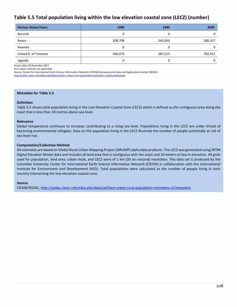
108
Table 5.5 Total population living within the low elevation coastal zone (LECZ) (number)
Partner States/Years 1990 1995 2000
Burundi 0 0 0
Kenya 208,708 245,839 280,327
Rwanda 0 0 0
United R. of Tanzania 566,079 687,213 782,912
Uganda 0 0 0
Access date: 04 December 2017
Zero values indicate not applicable
Source: Center for International Earth Science Information Network (CIESIN)/Socioeconomic Data and Applications Center (SEDAC) http://sedac.ciesin.columbia.edu/data/set/lecz-urban-rural-population-estimates-v1/data-download
Metadata for Table 5.5
Definition
Table 5.5 shows total population living in the Low Elevation Coastal Zone (LECZ) which is defined as the contiguous area along the
coast that is less than 10 metres above sea level.
Relevance
Global temperature continues to increase, contributing to a rising sea level. Populations living in the LECZ are under threat of
becoming environmental refugees. Data on the population living in the LECZ illustrate the number of people potentially at risk of
sea level rise.
Computation/Collection Method
All estimates are based on Global Rural-Urban Mapping Project (GRUMP) alpha data products. The LECZ was generated using SRTM
Digital Elevation Model data and includes all land area that is contiguous with the coast and 10 meters or less in elevation. All grids
used for population, land area, urban mask, and LECZ were of 1 km (30 arc-second) resolution. This data set is produced by the
Columbia University Center for International Earth Science Information Network (CIESIN) in collaboration with the International
Institute for Environment and Development (IIED). Total populations were calculated as the number of people living in each
country intersecting the low elevation coastal zone.
Source
CIESIN/SEDAC, http://sedac.ciesin.columbia.edu/data/set/lecz-urban-rural-population-estimates-v1/metadata
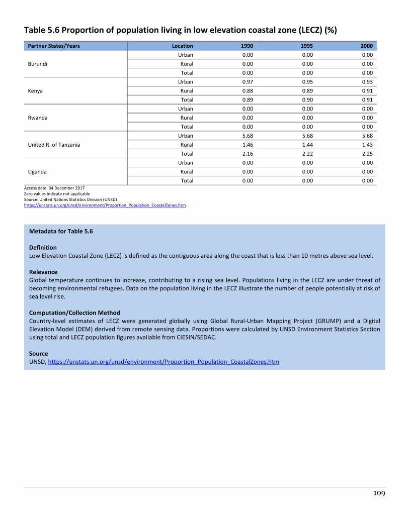
109
Table 5.6 Proportion of population living in low elevation coastal zone (LECZ) (%)
Partner States/Years Location 1990 1995 2000
Burundi
Urban 0.00 0.00 0.00
Rural 0.00 0.00 0.00
Total 0.00 0.00 0.00
Kenya
Urban 0.97 0.95 0.93
Rural 0.88 0.89 0.91
Total 0.89 0.90 0.91
Rwanda
Urban 0.00 0.00 0.00
Rural 0.00 0.00 0.00
Total 0.00 0.00 0.00
United R. of Tanzania
Urban 5.68 5.68 5.68
Rural 1.46 1.44 1.43
Total 2.16 2.22 2.25
Uganda
Urban 0.00 0.00 0.00
Rural 0.00 0.00 0.00
Total 0.00 0.00 0.00
Access date: 04 December 2017
Zero values indicate not applicable
Source: United Nations Statistics Division (UNSD)
https://unstats.un.org/unsd/environment/Proportion_Population_CoastalZones.htm
Metadata for Table 5.6
Definition
Low Elevation Coastal Zone (LECZ) is defined as the contiguous area along the coast that is less than 10 metres above sea level.
Relevance
Global temperature continues to increase, contributing to a rising sea level. Populations living in the LECZ are under threat of
becoming environmental refugees. Data on the population living in the LECZ illustrate the number of people potentially at risk of
sea level rise.
Computation/Collection Method
Country-level estimates of LECZ were generated globally using Global Rural-Urban Mapping Project (GRUMP) and a Digital
Elevation Model (DEM) derived from remote sensing data. Proportions were calculated by UNSD Environment Statistics Section
using total and LECZ population figures available from CIESIN/SEDAC.
Source
UNSD, https://unstats.un.org/unsd/environment/Proportion_Population_CoastalZones.htm
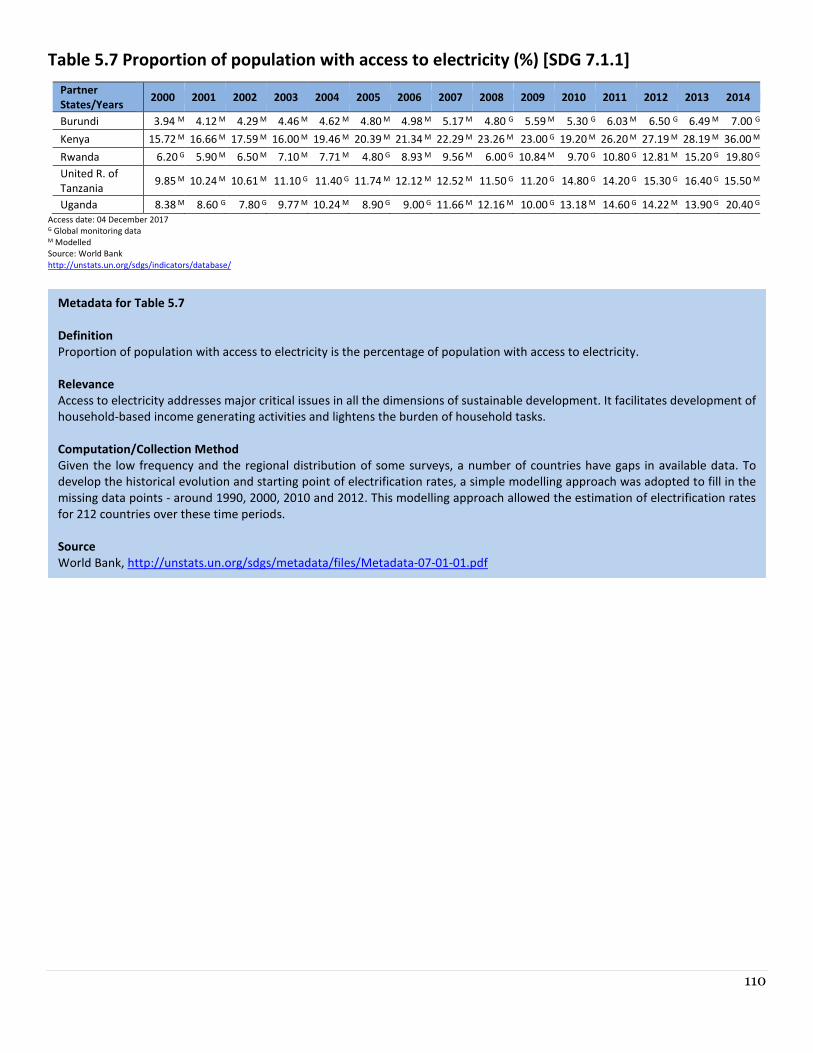
110
Table 5.7 Proportion of population with access to electricity (%) [SDG 7.1.1]
Partner
States/Years 2000 M 2001 M 2002 M 2003 M 2004 M 2005 M 2006 M 2007 M 2008 M 2009 M 2010 M 2011 M 2012 M 2013 M 2014 M
Burundi 3.94 M 4.12 M 4.29 M 4.46 M 4.62 M 4.80 M 4.98 M 5.17 M 4.80 G 5.59 M 5.30 G 6.03 M 6.50 G 6.49 M 7.00 G
Kenya 15.72 M 16.66 M 17.59 M 16.00 M 19.46 M 20.39 M 21.34 M 22.29 M 23.26 M 23.00 G 19.20 M 26.20 M 27.19 M 28.19 M 36.00 M
Rwanda 6.20 G 5.90 M 6.50 M 7.10 M 7.71 M 4.80 G 8.93 M 9.56 M 6.00 G 10.84 M 9.70 G 10.80 G 12.81 M 15.20 G 19.80 G
United R. of
Tanzania 9.85 M 10.24 M 10.61 M 11.10 G 11.40 G 11.74 M 12.12 M 12.52 M 11.50 G 11.20 G 14.80 G 14.20 G 15.30 G 16.40 G 15.50 M
Uganda 8.38 M 8.60 G 7.80 G 9.77 M 10.24 M 8.90 G 9.00 G 11.66 M 12.16 M 10.00 G 13.18 M 14.60 G 14.22 M 13.90 G 20.40 G
Access date: 04 December 2017 G Global monitoring data M Modelled
Source: World Bank
http://unstats.un.org/sdgs/indicators/database/
Metadata for Table 5.7
Definition
Proportion of population with access to electricity is the percentage of population with access to electricity.
Relevance
Access to electricity addresses major critical issues in all the dimensions of sustainable development. It facilitates development of
household-based income generating activities and lightens the burden of household tasks.
Computation/Collection Method
Given the low frequency and the regional distribution of some surveys, a number of countries have gaps in available data. To
develop the historical evolution and starting point of electrification rates, a simple modelling approach was adopted to fill in the
missing data points - around 1990, 2000, 2010 and 2012. This modelling approach allowed the estimation of electrification rates
for 212 countries over these time periods.
Source
World Bank, http://unstats.un.org/sdgs/metadata/files/Metadata-07-01-01.pdf
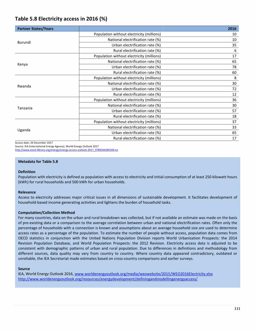
111
Table 5.8 Electricity access in 2016 (%)
Partner States/Years 2016
Burundi
Population without electricity (millions) 10
National electrification rate (%) 10
Urban electrification rate (%) 35
Rural electrification rate (%) 6
Kenya
Population without electricity (millions) 17
National electrification rate (%) 65
Urban electrification rate (%) 78
Rural electrification rate (%) 60
Rwanda
Population without electricity (millions) 8
National electrification rate (%) 30
Urban electrification rate (%) 72
Rural electrification rate (%) 12
Tanzania
Population without electricity (millions) 36
National electrification rate (%) 30
Urban electrification rate (%) 57
Rural electrification rate (%) 18
Uganda
Population without electricity (millions) 37
National electrification rate (%) 33
Urban electrification rate (%) 65
Rural electrification rate (%) 17 Access date: 26 December 2017
Source: IEA (International Energy Agency), World Energy Outlook 2017
http://www.oecd-ilibrary.org/energy/energy-access-outlook-2017_9789264285569-en
Metadata for Table 5.8
Definition
Population with electricity is defined as population with access to electricity and initial consumption of at least 250 kilowatt-hours
(kWh) for rural households and 500 kWh for urban households.
Relevance
Access to electricity addresses major critical issues in all dimensions of sustainable development. It facilitates development of
household-based income generating activities and lightens the burden of household tasks.
Computation/Collection Method
For many countries, data on the urban and rural breakdown was collected, but if not available an estimate was made on the basis
of pre-existing data or a comparison to the average correlation between urban and national electrification rates. Often only the
percentage of households with a connection is known and assumptions about an average household size are used to determine
access rates as a percentage of the population. To estimate the number of people without access, population data comes from
OECD statistics in conjunction with the United Nations Population Division reports World Urbanization Prospects: the 2014
Revision Population Database, and World Population Prospects: the 2012 Revision. Electricity access data is adjusted to be
consistent with demographic patterns of urban and rural population. Due to differences in definitions and methodology from
different sources, data quality may vary from country to country. Where country data appeared contradictory, outdated or
unreliable, the IEA Secretariat made estimates based on cross-country comparisons and earlier surveys.
Source
IEA, World Energy Outlook 2016, www.worldenergyoutlook.org/media/weowebsite/2015/WEO2016Electricity.xlsx
http://www.worldenergyoutlook.org/resources/energydevelopment/definingandmodellingenergyaccess/
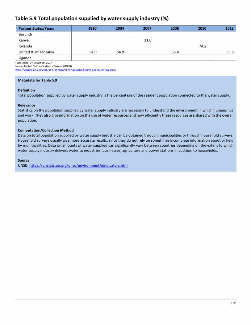
112
Table 5.9 Total population supplied by water supply industry (%)
Partner States/Years 1990 2004 2007 2008 2010 2013
Burundi
Kenya 31.0
Rwanda 74.2
United R. of Tanzania 54.0 54.9 55.4 55.6
Uganda Access date: 04 December 2017
Source: United Nations Statistics Division (UNSD)
https://unstats.un.org/unsd/environment/Time%20series.htm#InlandWaterResources
Metadata for Table 5.9
Definition
Total population supplied by water supply industry is the percentage of the resident population connected to the water supply.
Relevance
Statistics on the population supplied by water supply industry are necessary to understand the environment in which humans live
and work. They also give information on the use of water resources and how efficiently these resources are shared with the overall
population.
Computation/Collection Method
Data on total population supplied by water supply industry can be obtained through municipalities or through household surveys.
Household surveys usually give more accurate results, since they do not rely on sometimes incomplete information about or held
by municipalities. Data on amounts of water supplied can significantly vary between countries depending on the extent to which
water supply industry delivers water to industries, businesses, agriculture and power stations in addition to households.
Source
UNSD, https://unstats.un.org/unsd/environment/qindicators.htm
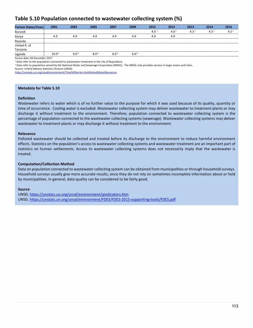
113
Table 5.10 Population connected to wastewater collecting system (%)
Partner States/Years 2001 2003 2005 2007 2009 2012 2012 2013 2014 2015
Burundi 4.0 1 4.0 1 4.5 1 4.5 1 4.5 1
Kenya 4.9 4.9 4.9 4.9 4.9 4.9 4.9
Rwanda
United R. of
Tanzania
Uganda 10.0 2 9.0 2 8.0 2 6.0 2 6.0 2
Access date: 04 December 2017 1 Data refer to the population connected to wastewater treatment in the city of Bujumbura. 2 Data refer to population served by the National Water and Sewerage Corporation (NWSC). The NWSC only provides service in larger towns and cities.
Source: United Nations Statistics Division (UNSD)
https://unstats.un.org/unsd/environment/Time%20series.htm#InlandWaterResources
Metadata for Table 5.10
Definition
Wastewater refers to water which is of no further value to the purpose for which it was used because of its quality, quantity or
time of occurrence. Cooling water is excluded. Wastewater collecting system may deliver wastewater to treatment plants or may
discharge it without treatment to the environment. Therefore, population connected to wastewater collecting system is the
percentage of population connected to the wastewater collecting systems (sewerage). Wastewater collecting systems may deliver
wastewater to treatment plants or may discharge it without treatment to the environment.
Relevance
Polluted wastewater should be collected and treated before its discharge to the environment to reduce harmful environment
effects. Statistics on the population’s access to wastewater collecting systems and wastewater treatment are an important part of
statistics on human settlements. Access to wastewater collecting systems does not necessarily imply that the wastewater is
treated.
Computation/Collection Method
Data on population connected to wastewater collecting system can be obtained from municipalities or through household surveys.
Household surveys usually give more accurate results, since they do not rely on sometimes incomplete information about or held
by municipalities. In general, data quality can be considered to be fairly good.
Source
UNSD, https://unstats.un.org/unsd/environment/qindicators.htm
UNSD, https://unstats.un.org/unsd/environment/FDES/FDES-2015-supporting-tools/FDES.pdf
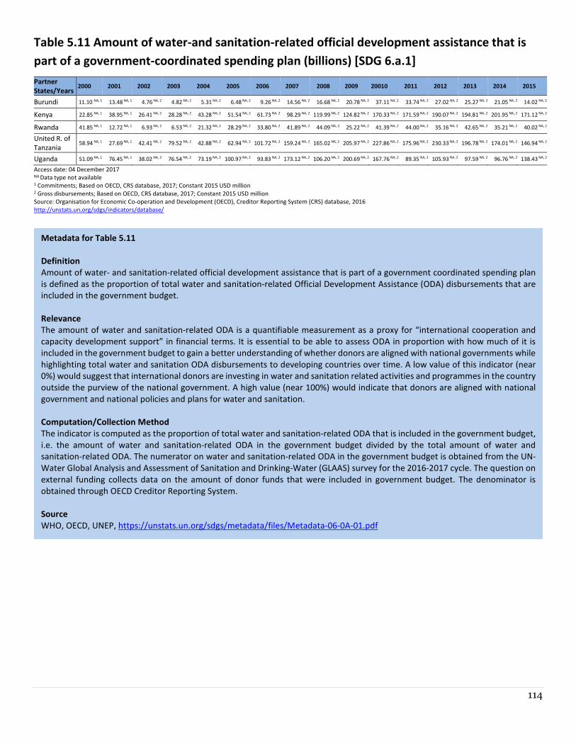
114
Table 5.11 Amount of water-and sanitation-related official development assistance that is
part of a government-coordinated spending plan (billions) [SDG 6.a.1]
Partner
States/Years 2000 NA, 1 2001 NA, 1 2002 NA, 1 2003 NA, 1 2004 NA, 1 2005 NA, 1 2006 NA, 1 2007 NA, 1 2008NA, 1 2009 NA, 1 20010 NA, 1 2011 NA, 1 2012 NA, 1 2013 NA, 1 2014 NA, 1 2015 NA, 1
Burundi 11.10 NA, 1 13.48 NA, 1 4.76 NA, 2 4.82 NA, 2 5.31 NA, 2 6.48 NA, 2 9.26 NA, 2 14.56 NA, 2 16.68 NA, 2 20.78 NA, 2 37.11 NA, 2 33.74 NA, 2 27.02 NA, 2 25.27 NA, 2 21.05 NA, 2 14.02 NA, 2
Kenya 22.85 NA, 1 38.95 NA, 1 26.41 NA, 2 28.28 NA, 2 43.28 NA, 2 51.54 NA, 2 61.73 NA, 2 98.29 NA, 2 119.99 NA, 2 124.82 NA, 2 170.33 NA, 2 171.59 NA, 2 190.07 NA, 2 194.81 NA, 2 201.95 NA, 2 171.12 NA, 2
Rwanda 41.85 NA, 1 12.72 NA, 1 6.93 NA, 2 6.53 NA, 2 21.32 NA, 2 28.29 NA, 2 33.80 NA, 2 41.89 NA, 2 44.09 NA, 2 25.22 NA, 2 41.39 NA, 2 44.00 NA, 2 35.16 NA, 2 42.65 NA, 2 35.21 NA, 2 40.02 NA, 2
United R. of
Tanzania 58.94 NA, 1 27.69 NA, 1 42.41 NA, 2 79.52 NA, 2 42.88 NA, 2 62.94 NA, 2 101.72 NA, 2 159.24 NA, 2 165.02 NA, 2 205.97 NA, 2 227.86 NA, 2 175.96 NA, 2 230.33 NA, 2 196.78 NA, 2 174.01 NA, 2 146.94 NA, 2
Uganda 51.09 NA, 1 76.45 NA, 1 38.02 NA, 2 76.54 NA, 2 73.19 NA, 2 100.97 NA, 2 93.83 NA, 2 173.12 NA, 2 106.20 NA, 2 200.69 NA, 2 167.76 NA, 2 89.35 NA, 2 105.93 NA, 2 97.59 NA, 2 96.76 NA, 2 138.43 NA, 2
Access date: 04 December 2017 NA Data type not available 1 Commitments; Based on OECD, CRS database, 2017; Constant 2015 USD million 2 Gross disbursements; Based on OECD, CRS database, 2017; Constant 2015 USD million
Source: Organisation for Economic Co-operation and Development (OECD), Creditor Reporting System (CRS) database, 2016
http://unstats.un.org/sdgs/indicators/database/
Metadata for Table 5.11
Definition
Amount of water- and sanitation-related official development assistance that is part of a government coordinated spending plan
is defined as the proportion of total water and sanitation-related Official Development Assistance (ODA) disbursements that are
included in the government budget.
Relevance
The amount of water and sanitation-related ODA is a quantifiable measurement as a proxy for “international cooperation and
capacity development support” in financial terms. It is essential to be able to assess ODA in proportion with how much of it is
included in the government budget to gain a better understanding of whether donors are aligned with national governments while
highlighting total water and sanitation ODA disbursements to developing countries over time. A low value of this indicator (near
0%) would suggest that international donors are investing in water and sanitation related activities and programmes in the country
outside the purview of the national government. A high value (near 100%) would indicate that donors are aligned with national
government and national policies and plans for water and sanitation.
Computation/Collection Method
The indicator is computed as the proportion of total water and sanitation-related ODA that is included in the government budget,
i.e. the amount of water and sanitation-related ODA in the government budget divided by the total amount of water and
sanitation-related ODA. The numerator on water and sanitation-related ODA in the government budget is obtained from the UN-
Water Global Analysis and Assessment of Sanitation and Drinking-Water (GLAAS) survey for the 2016-2017 cycle. The question on
external funding collects data on the amount of donor funds that were included in government budget. The denominator is
obtained through OECD Creditor Reporting System.
Source
WHO, OECD, UNEP, https://unstats.un.org/sdgs/metadata/files/Metadata-06-0A-01.pdf
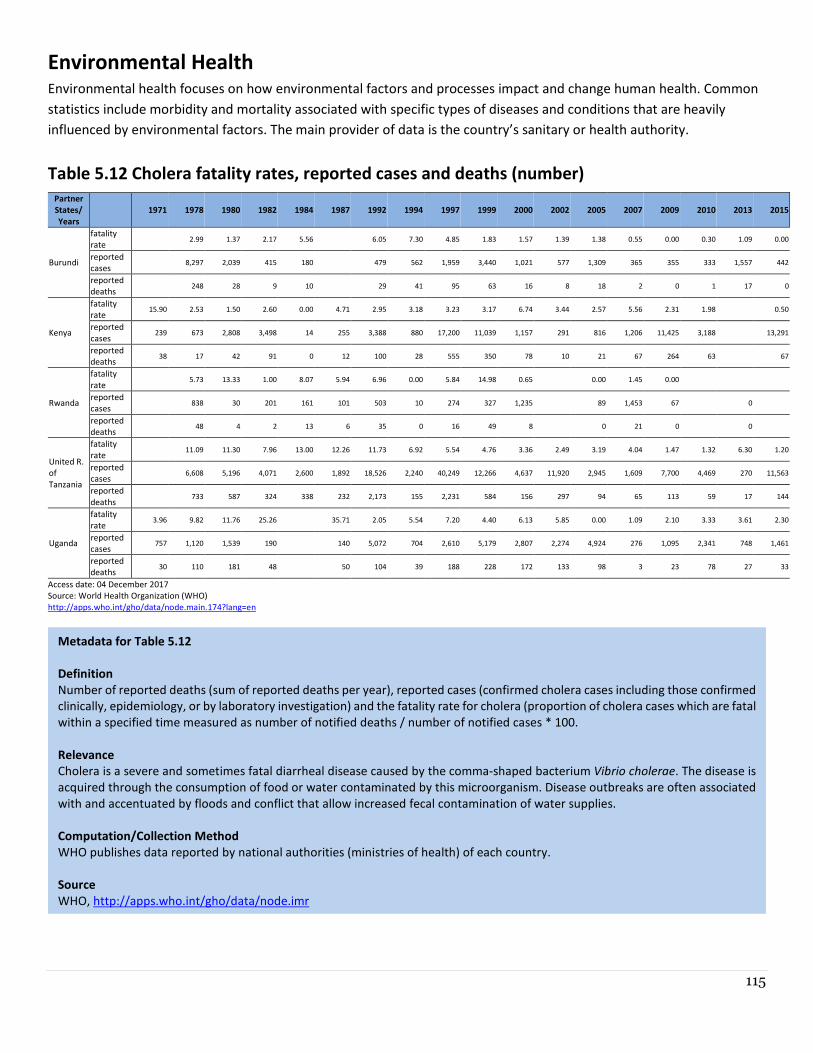
115
Environmental Health Environmental health focuses on how environmental factors and processes impact and change human health. Common
statistics include morbidity and mortality associated with specific types of diseases and conditions that are heavily
influenced by environmental factors. The main provider of data is the country’s sanitary or health authority.
Table 5.12 Cholera fatality rates, reported cases and deaths (number)
Partner
States/
Years
1971 1978 1980 1982 1984 1987 1992 1994 1997 1999 2000 2002 2005 2007 2009 2010 2013 2015
Burundi
fatality
rate 2.99 1.37 2.17 5.56 6.05 7.30 4.85 1.83 1.57 1.39 1.38 0.55 0.00 0.30 1.09 0.00
reported
cases 8,297 2,039 415 180 479 562 1,959 3,440 1,021 577 1,309 365 355 333 1,557 442
reported
deaths 248 28 9 10 29 41 95 63 16 8 18 2 0 1 17 0
Kenya
fatality
rate 15.90 2.53 1.50 2.60 0.00 4.71 2.95 3.18 3.23 3.17 6.74 3.44 2.57 5.56 2.31 1.98 0.50
reported
cases 239 673 2,808 3,498 14 255 3,388 880 17,200 11,039 1,157 291 816 1,206 11,425 3,188 13,291
reported
deaths 38 17 42 91 0 12 100 28 555 350 78 10 21 67 264 63 67
Rwanda
fatality
rate 5.73 13.33 1.00 8.07 5.94 6.96 0.00 5.84 14.98 0.65 0.00 1.45 0.00
reported
cases 838 30 201 161 101 503 10 274 327 1,235 89 1,453 67 0
reported
deaths 48 4 2 13 6 35 0 16 49 8 0 21 0 0
United R.
of
Tanzania
fatality
rate 11.09 11.30 7.96 13.00 12.26 11.73 6.92 5.54 4.76 3.36 2.49 3.19 4.04 1.47 1.32 6.30 1.20
reported
cases 6,608 5,196 4,071 2,600 1,892 18,526 2,240 40,249 12,266 4,637 11,920 2,945 1,609 7,700 4,469 270 11,563
reported
deaths 733 587 324 338 232 2,173 155 2,231 584 156 297 94 65 113 59 17 144
Uganda
fatality
rate 3.96 9.82 11.76 25.26 35.71 2.05 5.54 7.20 4.40 6.13 5.85 0.00 1.09 2.10 3.33 3.61 2.30
reported
cases 757 1,120 1,539 190 140 5,072 704 2,610 5,179 2,807 2,274 4,924 276 1,095 2,341 748 1,461
reported
deaths 30 110 181 48 50 104 39 188 228 172 133 98 3 23 78 27 33
Access date: 04 December 2017
Source: World Health Organization (WHO)
http://apps.who.int/gho/data/node.main.174?lang=en
Metadata for Table 5.12
Definition
Number of reported deaths (sum of reported deaths per year), reported cases (confirmed cholera cases including those confirmed
clinically, epidemiology, or by laboratory investigation) and the fatality rate for cholera (proportion of cholera cases which are fatal
within a specified time measured as number of notified deaths / number of notified cases * 100.
Relevance
Cholera is a severe and sometimes fatal diarrheal disease caused by the comma-shaped bacterium Vibrio cholerae. The disease is
acquired through the consumption of food or water contaminated by this microorganism. Disease outbreaks are often associated
with and accentuated by floods and conflict that allow increased fecal contamination of water supplies.
Computation/Collection Method
WHO publishes data reported by national authorities (ministries of health) of each country.
Source
WHO, http://apps.who.int/gho/data/node.imr
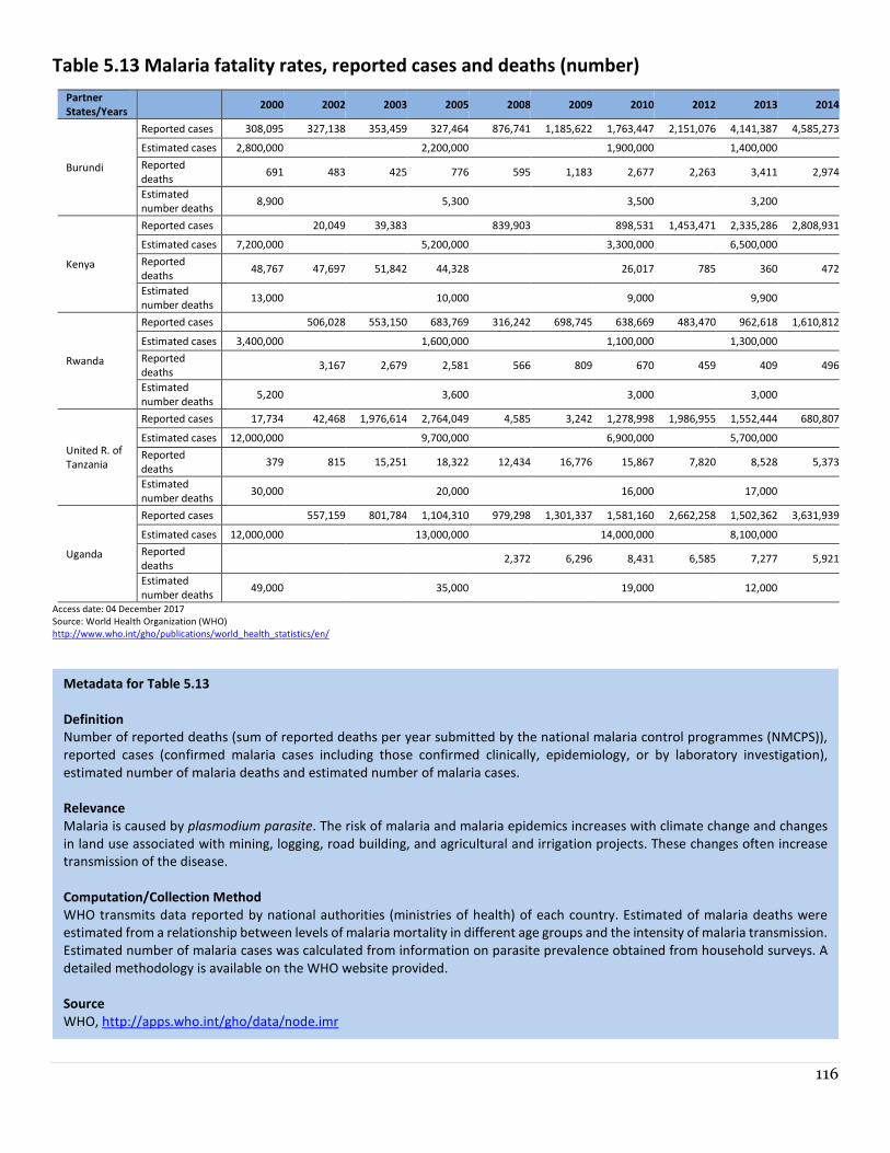
116
Table 5.13 Malaria fatality rates, reported cases and deaths (number)
Partner
States/Years 2000 2002 2003 2005 2008 2009 2010 2012 2013 2014
Burundi
Reported cases 308,095 327,138 353,459 327,464 876,741 1,185,622 1,763,447 2,151,076 4,141,387 4,585,273
Estimated cases 2,800,000 2,200,000 1,900,000 1,400,000
Reported
deaths 691 483 425 776 595 1,183 2,677 2,263 3,411 2,974
Estimated
number deaths 8,900 5,300 3,500 3,200
Kenya
Reported cases 20,049 39,383 839,903 898,531 1,453,471 2,335,286 2,808,931
Estimated cases 7,200,000 5,200,000 3,300,000 6,500,000
Reported
deaths 48,767 47,697 51,842 44,328 26,017 785 360 472
Estimated
number deaths 13,000 10,000 9,000 9,900
Rwanda
Reported cases 506,028 553,150 683,769 316,242 698,745 638,669 483,470 962,618 1,610,812
Estimated cases 3,400,000 1,600,000 1,100,000 1,300,000
Reported
deaths 3,167 2,679 2,581 566 809 670 459 409 496
Estimated
number deaths 5,200 3,600 3,000 3,000
United R. of
Tanzania
Reported cases 17,734 42,468 1,976,614 2,764,049 4,585 3,242 1,278,998 1,986,955 1,552,444 680,807
Estimated cases 12,000,000 9,700,000 6,900,000 5,700,000
Reported
deaths 379 815 15,251 18,322 12,434 16,776 15,867 7,820 8,528 5,373
Estimated
number deaths 30,000 20,000 16,000 17,000
Uganda
Reported cases 557,159 801,784 1,104,310 979,298 1,301,337 1,581,160 2,662,258 1,502,362 3,631,939
Estimated cases 12,000,000 13,000,000 14,000,000 8,100,000
Reported
deaths 2,372 6,296 8,431 6,585 7,277 5,921
Estimated
number deaths 49,000 35,000 19,000 12,000
Access date: 04 December 2017
Source: World Health Organization (WHO)
http://www.who.int/gho/publications/world_health_statistics/en/
Metadata for Table 5.13
Definition
Number of reported deaths (sum of reported deaths per year submitted by the national malaria control programmes (NMCPS)),
reported cases (confirmed malaria cases including those confirmed clinically, epidemiology, or by laboratory investigation),
estimated number of malaria deaths and estimated number of malaria cases.
Relevance
Malaria is caused by plasmodium parasite. The risk of malaria and malaria epidemics increases with climate change and changes
in land use associated with mining, logging, road building, and agricultural and irrigation projects. These changes often increase
transmission of the disease.
Computation/Collection Method
WHO transmits data reported by national authorities (ministries of health) of each country. Estimated of malaria deaths were
estimated from a relationship between levels of malaria mortality in different age groups and the intensity of malaria transmission.
Estimated number of malaria cases was calculated from information on parasite prevalence obtained from household surveys. A
detailed methodology is available on the WHO website provided.
Source
WHO, http://apps.who.int/gho/data/node.imr
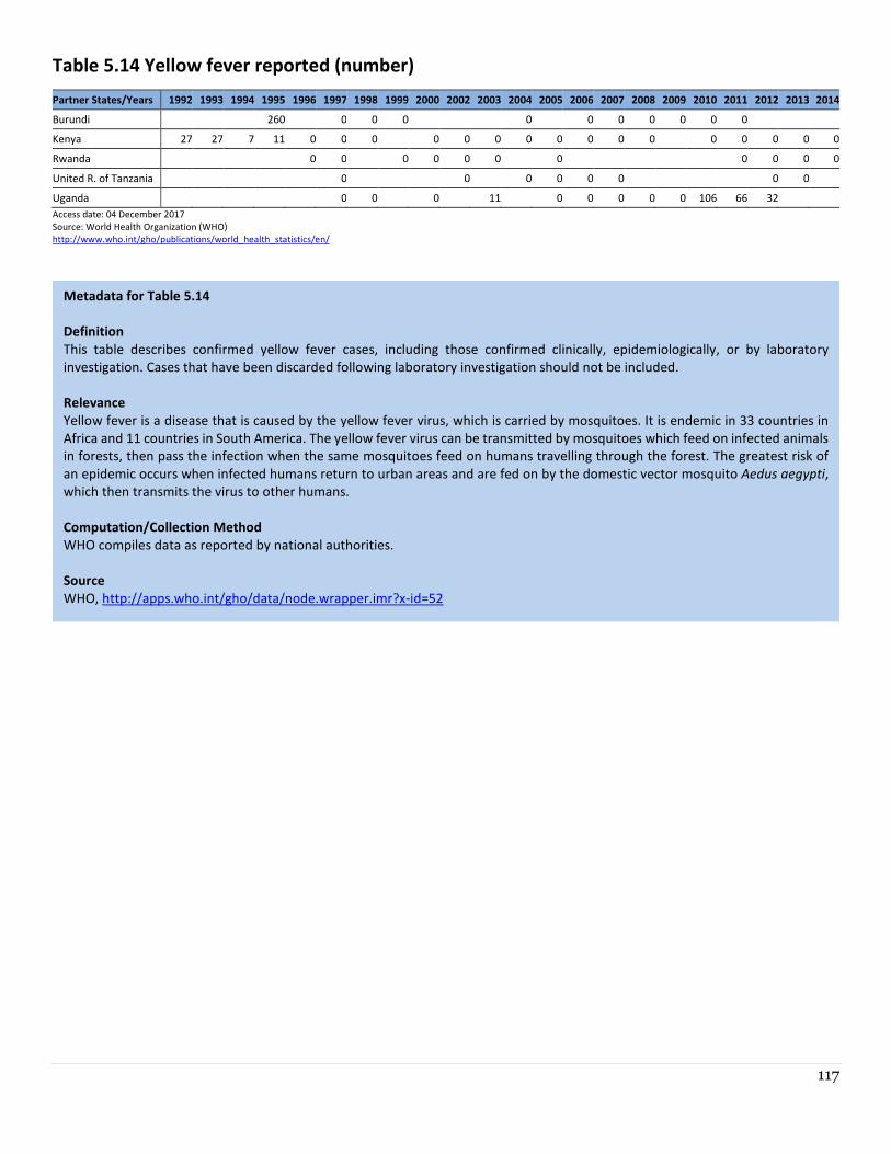
117
Table 5.14 Yellow fever reported (number)
Partner States/Years 1992 1993 1994 1995 1996 1997 1998 1999 2000 2002 2003 2004 2005 2006 2007 2008 2009 2010 2011 2012 2013 2014
Burundi 260 0 0 0 0 0 0 0 0 0 0
Kenya 27 27 7 11 0 0 0 0 0 0 0 0 0 0 0 0 0 0 0 0
Rwanda 0 0 0 0 0 0 0 0 0 0 0
United R. of Tanzania 0 0 0 0 0 0 0 0
Uganda 0 0 0 11 0 0 0 0 0 106 66 32
Access date: 04 December 2017
Source: World Health Organization (WHO)
http://www.who.int/gho/publications/world_health_statistics/en/
Metadata for Table 5.14
Definition
This table describes confirmed yellow fever cases, including those confirmed clinically, epidemiologically, or by laboratory
investigation. Cases that have been discarded following laboratory investigation should not be included.
Relevance
Yellow fever is a disease that is caused by the yellow fever virus, which is carried by mosquitoes. It is endemic in 33 countries in
Africa and 11 countries in South America. The yellow fever virus can be transmitted by mosquitoes which feed on infected animals
in forests, then pass the infection when the same mosquitoes feed on humans travelling through the forest. The greatest risk of
an epidemic occurs when infected humans return to urban areas and are fed on by the domestic vector mosquito Aedus aegypti,
which then transmits the virus to other humans.
Computation/Collection Method
WHO compiles data as reported by national authorities.
Source
WHO, http://apps.who.int/gho/data/node.wrapper.imr?x-id=52
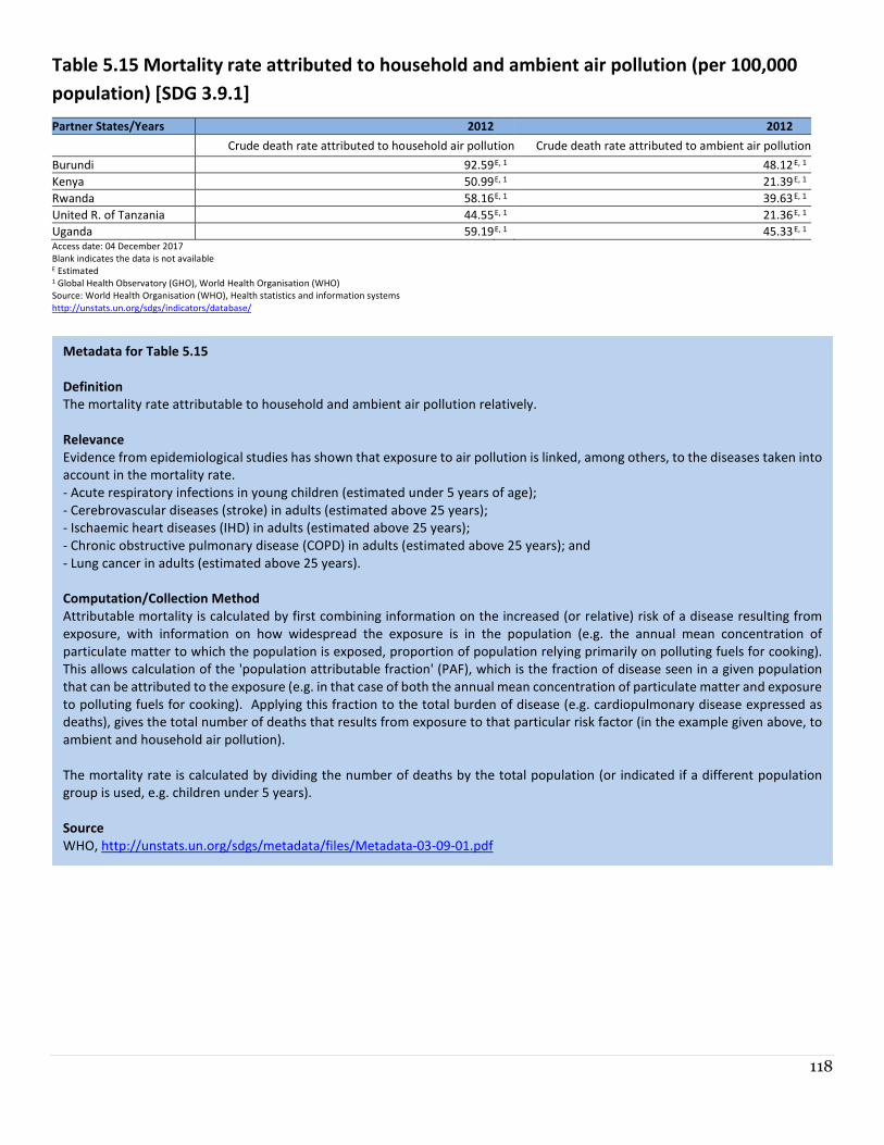
118
Table 5.15 Mortality rate attributed to household and ambient air pollution (per 100,000
population) [SDG 3.9.1]
Partner States/Years 2012 2012
Crude death rate attributed to household air pollution Crude death rate attributed to ambient air pollution
Burundi 92.59 E, 1 48.12 E, 1
Kenya 50.99 E, 1 21.39 E, 1
Rwanda 58.16 E, 1 39.63 E, 1
United R. of Tanzania 44.55 E, 1 21.36 E, 1
Uganda 59.19 E, 1 45.33 E, 1 Access date: 04 December 2017
Blank indicates the data is not available E Estimated 1 Global Health Observatory (GHO), World Health Organisation (WHO)
Source: World Health Organisation (WHO), Health statistics and information systems
http://unstats.un.org/sdgs/indicators/database/
Metadata for Table 5.15
Definition
The mortality rate attributable to household and ambient air pollution relatively.
Relevance
Evidence from epidemiological studies has shown that exposure to air pollution is linked, among others, to the diseases taken into
account in the mortality rate.
- Acute respiratory infections in young children (estimated under 5 years of age);
- Cerebrovascular diseases (stroke) in adults (estimated above 25 years);
- Ischaemic heart diseases (IHD) in adults (estimated above 25 years);
- Chronic obstructive pulmonary disease (COPD) in adults (estimated above 25 years); and
- Lung cancer in adults (estimated above 25 years).
Computation/Collection Method
Attributable mortality is calculated by first combining information on the increased (or relative) risk of a disease resulting from
exposure, with information on how widespread the exposure is in the population (e.g. the annual mean concentration of
particulate matter to which the population is exposed, proportion of population relying primarily on polluting fuels for cooking).
This allows calculation of the 'population attributable fraction' (PAF), which is the fraction of disease seen in a given population
that can be attributed to the exposure (e.g. in that case of both the annual mean concentration of particulate matter and exposure
to polluting fuels for cooking). Applying this fraction to the total burden of disease (e.g. cardiopulmonary disease expressed as
deaths), gives the total number of deaths that results from exposure to that particular risk factor (in the example given above, to
ambient and household air pollution).
The mortality rate is calculated by dividing the number of deaths by the total population (or indicated if a different population
group is used, e.g. children under 5 years).
Source
WHO, http://unstats.un.org/sdgs/metadata/files/Metadata-03-09-01.pdf
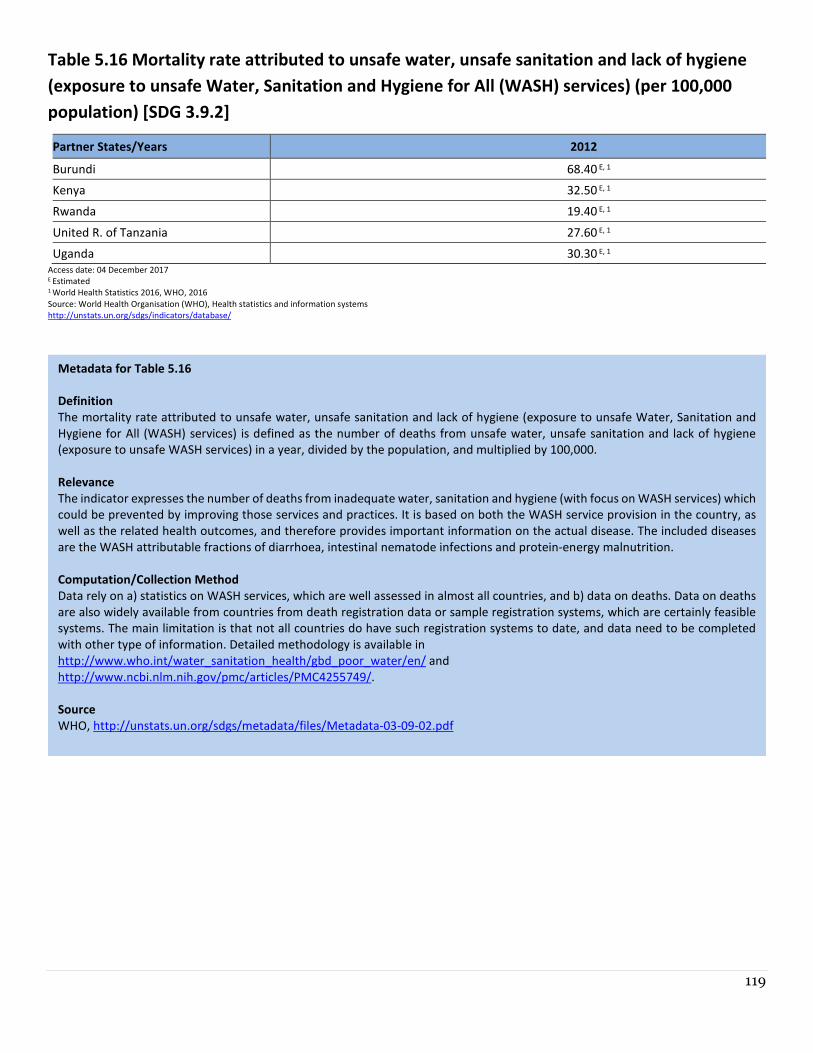
119
Table 5.16 Mortality rate attributed to unsafe water, unsafe sanitation and lack of hygiene
(exposure to unsafe Water, Sanitation and Hygiene for All (WASH) services) (per 100,000
population) [SDG 3.9.2]
Partner States/Years 2012
Burundi 68.40 E, 1
Kenya 32.50 E, 1
Rwanda 19.40 E, 1
United R. of Tanzania 27.60 E, 1
Uganda 30.30 E, 1
Access date: 04 December 2017 E Estimated 1 World Health Statistics 2016, WHO, 2016
Source: World Health Organisation (WHO), Health statistics and information systems
http://unstats.un.org/sdgs/indicators/database/
Metadata for Table 5.16
Definition
The mortality rate attributed to unsafe water, unsafe sanitation and lack of hygiene (exposure to unsafe Water, Sanitation and
Hygiene for All (WASH) services) is defined as the number of deaths from unsafe water, unsafe sanitation and lack of hygiene
(exposure to unsafe WASH services) in a year, divided by the population, and multiplied by 100,000.
Relevance
The indicator expresses the number of deaths from inadequate water, sanitation and hygiene (with focus on WASH services) which
could be prevented by improving those services and practices. It is based on both the WASH service provision in the country, as
well as the related health outcomes, and therefore provides important information on the actual disease. The included diseases
are the WASH attributable fractions of diarrhoea, intestinal nematode infections and protein-energy malnutrition.
Computation/Collection Method
Data rely on a) statistics on WASH services, which are well assessed in almost all countries, and b) data on deaths. Data on deaths
are also widely available from countries from death registration data or sample registration systems, which are certainly feasible
systems. The main limitation is that not all countries do have such registration systems to date, and data need to be completed
with other type of information. Detailed methodology is available in
http://www.who.int/water_sanitation_health/gbd_poor_water/en/ and
http://www.ncbi.nlm.nih.gov/pmc/articles/PMC4255749/.
Source
WHO, http://unstats.un.org/sdgs/metadata/files/Metadata-03-09-02.pdf
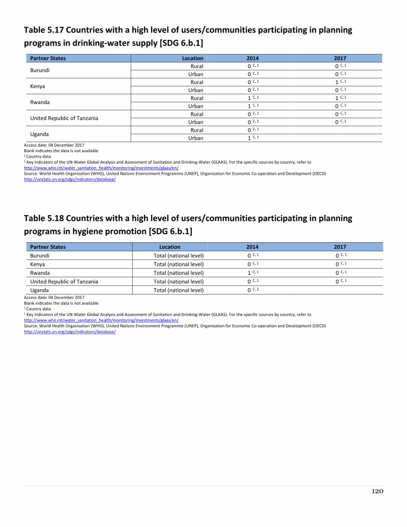
120
Table 5.17 Countries with a high level of users/communities participating in planning
programs in drinking-water supply [SDG 6.b.1]
Partner States Location 2014 2017
Burundi Rural 0 C, 1 0 C, 1
Urban 0 C, 1 0 C, 1
Kenya Rural 0 C, 1 1 C, 1
Urban 0 C, 1 0 C, 1
Rwanda Rural 1 C, 1 1 C, 1
Urban 1 C, 1 0 C, 1
United Republic of Tanzania Rural 0 C, 1 0 C, 1
Urban 0 C, 1 0 C, 1
Uganda Rural 0 C, 1
Urban 1 C, 1
Access date: 04 December 2017
Blank indicates the data is not available C Country data 1 Key indicators of the UN-Water Global Analysis and Assessment of Sanitation and Drinking-Water (GLAAS). For the specific sources by country, refer to
http://www.who.int/water_sanitation_health/monitoring/investments/glaas/en/
Source: World Health Organisation (WHO), United Nations Environment Programme (UNEP), Organisation for Economic Co-operation and Development (OECD)
http://unstats.un.org/sdgs/indicators/database/
Table 5.18 Countries with a high level of users/communities participating in planning
programs in hygiene promotion [SDG 6.b.1]
Partner States Location 2014 2017
Burundi Total (national level) 0 C, 1 0 C, 1
Kenya Total (national level) 0 C, 1 0 C, 1
Rwanda Total (national level) 1 C, 1 0 C, 1
United Republic of Tanzania Total (national level) 0 C, 1 0 C, 1
Uganda Total (national level) 0 C, 1
Access date: 04 December 2017
Blank indicates the data is not available C Country data 1 Key indicators of the UN-Water Global Analysis and Assessment of Sanitation and Drinking-Water (GLAAS). For the specific sources by country, refer to
http://www.who.int/water_sanitation_health/monitoring/investments/glaas/en/
Source: World Health Organisation (WHO), United Nations Environment Programme (UNEP), Organisation for Economic Co-operation and Development (OECD)
http://unstats.un.org/sdgs/indicators/database/
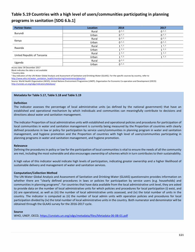
121
Table 5.19 Countries with a high level of users/communities participating in planning
programs in sanitation [SDG 6.b.1]
Partner States Location 2014 2017
Burundi Rural 0 C, 1 0 C, 1
Urban 0 C, 1 0 C, 1
Kenya Rural 0 C, 1 0 C, 1
Urban 0 C, 1 0 C, 1
Rwanda Rural 1 C, 1 1 C, 1
Urban 1 C, 1 1 C, 1
United Republic of Tanzania Rural 1 C, 1 1 C, 1
Urban 1 C, 1 1 C, 1
Uganda Rural 0 C, 1
Urban 0 C, 1
Access date: 04 December 2017
Blank indicates the data is not available C Country data 1 Key indicators of the UN-Water Global Analysis and Assessment of Sanitation and Drinking-Water (GLAAS). For the specific sources by country, refer to
http://www.who.int/water_sanitation_health/monitoring/investments/glaas/en/
Source: World Health Organisation (WHO), United Nations Environment Programme (UNEP), Organisation for Economic Co-operation and Development (OECD)
http://unstats.un.org/sdgs/indicators/database/
Metadata for Table 5.17, Table 5.18 and Table 5.19
Definition
The indicator assesses the percentage of local administrative units (as defined by the national government) that have an
established and operational mechanism by which individuals and communities can meaningfully contribute to decisions and
directions about water and sanitation management.
The indicator Proportion of local administrative units with established and operational policies and procedures for participation of
local communities in water and sanitation management is currently being measured by the Proportion of countries with clearly
defined procedures in law or policy for participation by service users/communities in planning program in water and sanitation
management, and hygiene promotion and the Proportion of countries with high level of users/communities participating in
planning programs in water and sanitation management, and hygiene promotion.
Relevance
Defining the procedures in policy or law for the participation of local communities is vital to ensure the needs of all the community
are met, including the most vulnerable and also encourages ownership of schemes which in turn contributes to their sustainability.
A high value of this indicator would indicate high levels of participation, indicating greater ownership and a higher likelihood of
sustainable delivery and management of water and sanitation services.
Computation/Collection Method
The UN-Water Global Analysis and Assessment of Sanitation and Drinking-Water (GLAAS) questionnaire provides information on
whether there are “clearly defined procedures in laws or policies for participation by service users (e.g. households) and
communities in planning programs”. For countries that have data available from the local administrative unit level, they are asked
to provide data on the number of local administrative units for which policies and procedures for local participation (i) exist, and
(ii) are operational, as well as (iii) the number of local administrative units assessed, and (iv) the total number of units in the
country. The indicator is computed as (ii) the number of local admin units with operation policies and procedures for local
participation divided by (iv) the total number of local administrative units in the country. Both numerator and denominator will be
obtained through the GLAAS survey for the 2016-2017 cycle.
Source
WHO, UNEP, OECD, https://unstats.un.org/sdgs/metadata/files/Metadata-06-0B-01.pdf

122
Chapter 6 Environmental Protection
Management and Engagement
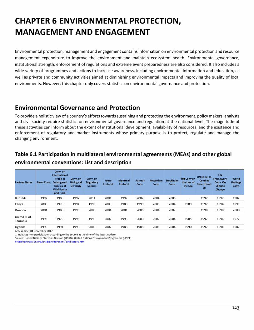
123
CHAPTER 6 ENVIRONMENTAL PROTECTION,
MANAGEMENT AND ENGAGEMENT
Environmental protection, management and engagement contains information on environmental protection and resource
management expenditure to improve the environment and maintain ecosystem health. Environmental governance,
institutional strength, enforcement of regulations and extreme event preparedness are also considered. It also includes a
wide variety of programmes and actions to increase awareness, including environmental information and education, as
well as private and community activities aimed at diminishing environmental impacts and improving the quality of local
environments. However, this chapter only covers statistics on environmental governance and protection.
Environmental Governance and Protection To provide a holistic view of a country’s efforts towards sustaining and protecting the environment, policy makers, analysts
and civil society require statistics on environmental governance and regulation at the national level. The magnitude of
these activities can inform about the extent of institutional development, availability of resources, and the existence and
enforcement of regulatory and market instruments whose primary purpose is to protect, regulate and manage the
changing environment.
Table 6.1 Participation in multilateral environmental agreements (MEAs) and other global
environmental conventions: List and description
Partner States Basel Conv.
Conv. on
International
Trade in
Endangered
Species of
Wild Fauna
and Flora
Conv. on
Biological
Diversity
Conv. on
Migratory
Species
Kyoto
Protocol
Montreal
Protocol
Ramsar
Conv.
Rotterdam
Conv.
Stockholm
Conv.
UN Conv on
the Law of
the Sea
UN Conv. to
Combat
Desertificati
on
UN
Framework
Conv. On
Climate
Change
World
Heritage
Conv.
Burundi 1997 1988 1997 2011 2001 1997 2002 2004 2005 ... 1997 1997 1982
Kenya 2000 1978 1994 1999 2005 1988 1990 2005 2004 1989 1997 1994 1991
Rwanda 2004 1980 1996 2005 2004 2001 2006 2004 2002 ... 1998 1998 2000
United R. of
Tanzania 1993 1979 1996 1999 2002 1993 2000 2002 2004 1985 1997 1996 1977
Uganda 1999 1991 1993 2000 2002 1988 1988 2008 2004 1990 1997 1994 1987
Access date: 04 December 2017
… indicates non-participation according to the source at the time of the latest update
Source: United Nations Statistics Division (UNSD), United Nations Environment Programme (UNEP)
https://unstats.un.org/unsd/environment/qindicators.htm
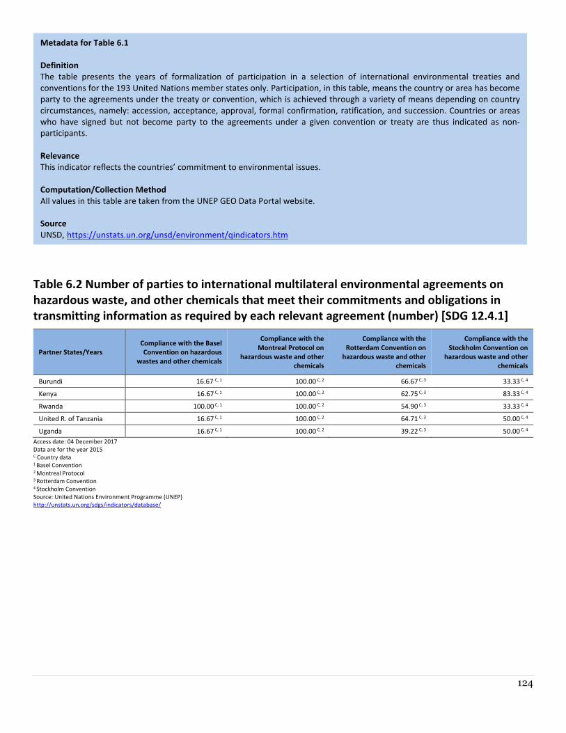
124
Table 6.2 Number of parties to international multilateral environmental agreements on
hazardous waste, and other chemicals that meet their commitments and obligations in
transmitting information as required by each relevant agreement (number) [SDG 12.4.1]
Partner States/Years
Compliance with the Basel
Convention on hazardous
wastes and other chemicals
Compliance with the
Montreal Protocol on
hazardous waste and other
chemicals
Compliance with the
Rotterdam Convention on
hazardous waste and other
chemicals
Compliance with the
Stockholm Convention on
hazardous waste and other
chemicals
Burundi 16.67 C, 1 100.00 C, 2 66.67 C, 3 33.33 C, 4
Kenya 16.67 C, 1 100.00 C, 2 62.75 C, 3 83.33 C, 4
Rwanda 100.00 C, 1 100.00 C, 2 54.90 C, 3 33.33 C, 4
United R. of Tanzania 16.67 C, 1 100.00 C, 2 64.71 C, 3 50.00 C, 4
Uganda 16.67 C, 1 100.00 C, 2 39.22 C, 3 50.00 C, 4
Access date: 04 December 2017
Data are for the year 2015 C Country data 1 Basel Convention 2 Montreal Protocol 3 Rotterdam Convention 4 Stockholm Convention
Source: United Nations Environment Programme (UNEP)
http://unstats.un.org/sdgs/indicators/database/
Metadata for Table 6.1
Definition
The table presents the years of formalization of participation in a selection of international environmental treaties and
conventions for the 193 United Nations member states only. Participation, in this table, means the country or area has become
party to the agreements under the treaty or convention, which is achieved through a variety of means depending on country
circumstances, namely: accession, acceptance, approval, formal confirmation, ratification, and succession. Countries or areas
who have signed but not become party to the agreements under a given convention or treaty are thus indicated as non-
participants.
Relevance
This indicator reflects the countries’ commitment to environmental issues.
Computation/Collection Method
All values in this table are taken from the UNEP GEO Data Portal website.
Source
UNSD, https://unstats.un.org/unsd/environment/qindicators.htm
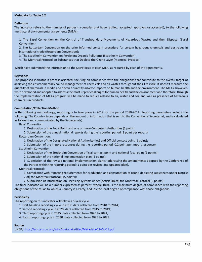
125
Metadata for Table 6.2
Definition
The indicator refers to the number of parties (=countries that have ratified, accepted, approved or accessed), to the following
multilateral environmental agreements (MEAs):
1. The Basel Convention on the Control of Transboundary Movements of Hazardous Wastes and their Disposal (Basel
Convention);
2. The Rotterdam Convention on the prior informed consent procedure for certain hazardous chemicals and pesticides in
international trade (Rotterdam Convention);
3. The Stockholm Convention on Persistent Organic Pollutants (Stockholm Convention);
4. The Montreal Protocol on Substances that Deplete the Ozone Layer (Montreal Protocol),
Which have submitted the information to the Secretariat of each MEA, as required by each of the agreements.
Relevance
The proposed indicator is process-oriented, focusing on compliance with the obligations that contribute to the overall target of
achieving the environmentally sound management of chemicals and all wastes throughout their life cycle. It doesn’t measure the
quantity of chemicals in media and doesn’t quantify adverse impacts on human health and the environment. The MEAs, however,
were developed and adopted to address the most urgent challenges for human health and the environment and therefore, through
the implementation of MEAs progress will be made to reduce release to air, water and soil and well as presence of hazardous
chemicals in products.
Computation/Collection Method
In the following methodology, reporting is to take place in 2017 for the period 2010-2014. Reporting parameters include the
following: The Country Score depends on the amount of information that is sent to the Conventions’ Secretariat, and is calculated
as follows (and communicated by the Secretariats):
Basel Convention:
1. Designation of the Focal Point and one or more Competent Authorities (1 point);
2. Submission of the annual national reports during the reporting period (1 point per report).
Rotterdam Convention:
1. Designation of the Designated National Authority(-ies) and Official contact point (1 point);
2. Submission of the import responses during the reporting period (0,2 point per import response).
Stockholm Convention:
1. Designation of the Stockholm Convention official contact point and national focal point (1 points);
2. Submission of the national implementation plan (1 points);
3. Submission of the revised national implementation plan(s) addressing the amendments adopted by the Conference of
the Parties within the reporting period (1 point per revised and updated plan).
Montreal Protocol:
1. Compliance with reporting requirements for production and consumption of ozone-depleting substances under (Article
7 of) the Montreal Protocol (15 points);
2. Submission of information on Licensing systems under (Article 4B of) the Montreal Protocol (5 points).
The final indicator will be a number expressed as percent, where 100% is the maximum degree of compliance with the reporting
obligations of the MEAs to which a Country is a Party, and 0% the least degree of compliance with those obligations.
Periodicity
The reporting on this indicator will follow a 5-year cycle.
1. First baseline reporting cycle in 2017: data collected from 2010 to 2014;
2. Second reporting cycle in 2020: data collected from 2015 to 2019;
3. Third reporting cycle in 2025: data collected from 2020 to 2024;
4. Fourth reporting cycle in 2030: data collected from 2025 to 2029.
Source
UNEP, https://unstats.un.org/sdgs/metadata/files/Metadata-12-04-01.pdf

126
127
N


![EAST AFRICAN STANDARD - EAC · PDF fileEAST AFRICAN STANDARD Fresh okra — Specification and grading EAST AFRICAN COMMUNITY HS 0709.90.00 [HS 0709.90.40] Draft](https://img.pdfslide.us/doc/110x75/5ab887377f8b9ad3038ce9a7/east-african-standard-eac-african-standard-fresh-okra-specification-and-grading.jpg)