Embed Size (px)
Citation preview
E. T. S. I. Caminos, Canales y Puertos 1
Gauss Jordan
2
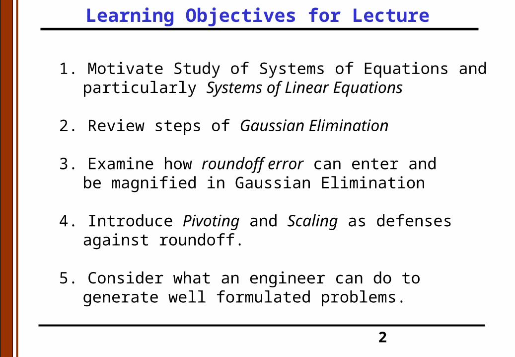
1. Motivate Study of Systems of Equations and particularly Systems of Linear Equations
2. Review steps of Gaussian Elimination
3. Examine how roundoff error can enter andbe magnified in Gaussian Elimination
4. Introduce Pivoting and Scaling as defenses against roundoff.
5. Consider what an engineer can do to generate well formulated problems.
Learning Objectives for Lecture
3
Systems of Equations
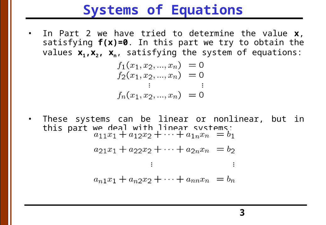
• In Part 2 we have tried to determine the value x, satisfying f(x)=0. In this part we try to obtain the values x1,x2, xn, satisfying the system of equations:
• These systems can be linear or nonlinear, but in this part we deal with linear systems:
4
Systems of Equations
• where a and b are constant coefficients, and n is the number of equations.
• Many of the engineering fundamental equations are based on conservation laws. In mathematical terms, these principles lead to balance or continuity equations relating the system behavior with respect to the amount of the magnitude being modelled and the extrenal stimuli acting on the system.
5
Systems of Equations
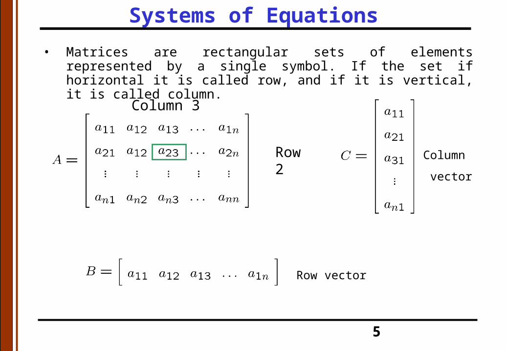
• Matrices are rectangular sets of elements represented by a single symbol. If the set if horizontal it is called row, and if it is vertical, it is called column.
Row 2
Column 3
Row vector
Column
vector

6
Systems of Equations
• There are some special types of matrices:
Symmetric matrix Identity matrix
Diagonal matrix Upper triangular matrix
7
Systems of Equations
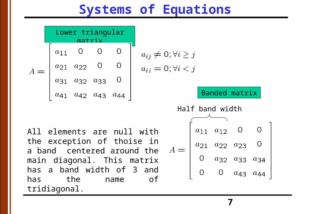
Banded matrix
All elements are null with the exception of thoise in a band centered around the main diagonal. This matrix has a band width of 3 and has the name of tridiagonal.
Half band width
Lower triangular matrix
8
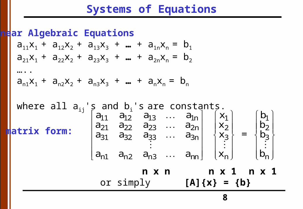
Linear Algebraic Equationsa11x1 + a12x2 + a13x3 + … + a1nxn = b1
a21x1 + a22x2 + a23x3 + … + a2nxn = b2
…..an1x1 + an2x2 + an3x3 + … + anxn = bn
where all aij's and bi's are constants.
In matrix form:
11 12 13 1n 1 121 22 23 2n 2 2
3 331 32 33 3n
n nn1 n2 n3 nn
a a a a x ba a a a x b
= x ba a a a
x ba a a a
n x n n x 1 n x 1or simply [A]{x} = {b}
Systems of Equations

9
Systems of Equations
• Matrix representation of a system
Matrix product:
Resulting dimensions

10
Systems of Equations
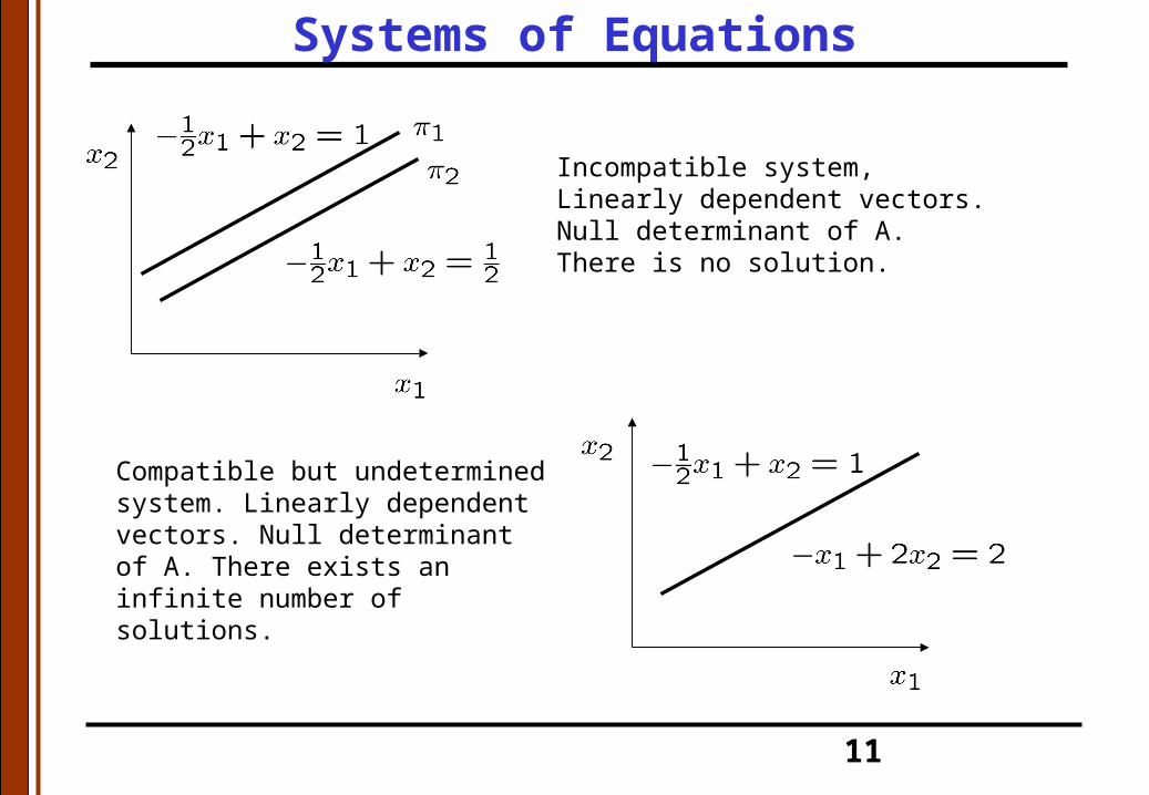
• Graphic Solution: Systems of equations are hyperplanes (straight lines, planes, etc.). The solution of a system is the intersection of these hyperplanes.
Compatible and determined system. Vectors are linearly independent. Unique solution. Determinant of A is non-null.
11
Systems of Equations
Incompatible system, Linearly dependent vectors. Null determinant of A. There is no solution.
Compatible but undetermined system. Linearly dependent vectors. Null determinant of A. There exists an infinite number of solutions.
12
Systems of Equations
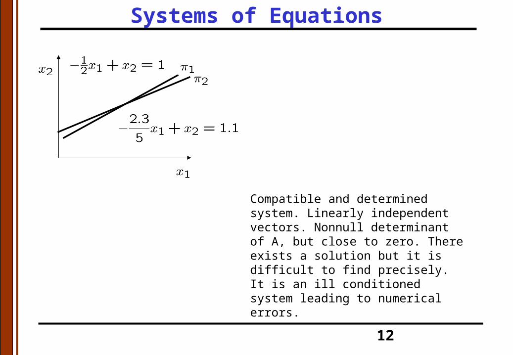
Compatible and determined system. Linearly independent vectors. Nonnull determinant of A, but close to zero. There exists a solution but it is difficult to find precisely. It is an ill conditioned system leading to numerical errors.

13
Gauss elimination• Naive Gauss elimination method: The Gauss’ method has two phases:
Forward elimination and backsustitution. In the first, the system is reduced to an upper triangular system:
• First, the unknown x1 is eliminated. To this end, the first row is multiplied by -a21/a11 and added to the second row. The same is done with all other succesive rows (n-1 times) until only the first equation contains the first unknown x1.
Pivotequation
substract
pivot

14
Gauss elimination
• This operation is repeated with all variables xi, until an upper triangular matrix is obtained.
• Next, the system is solved by backsustitution.
• The number of operations (FLOPS) used in the Gauss method is:
Pass 1 Pass 2
15
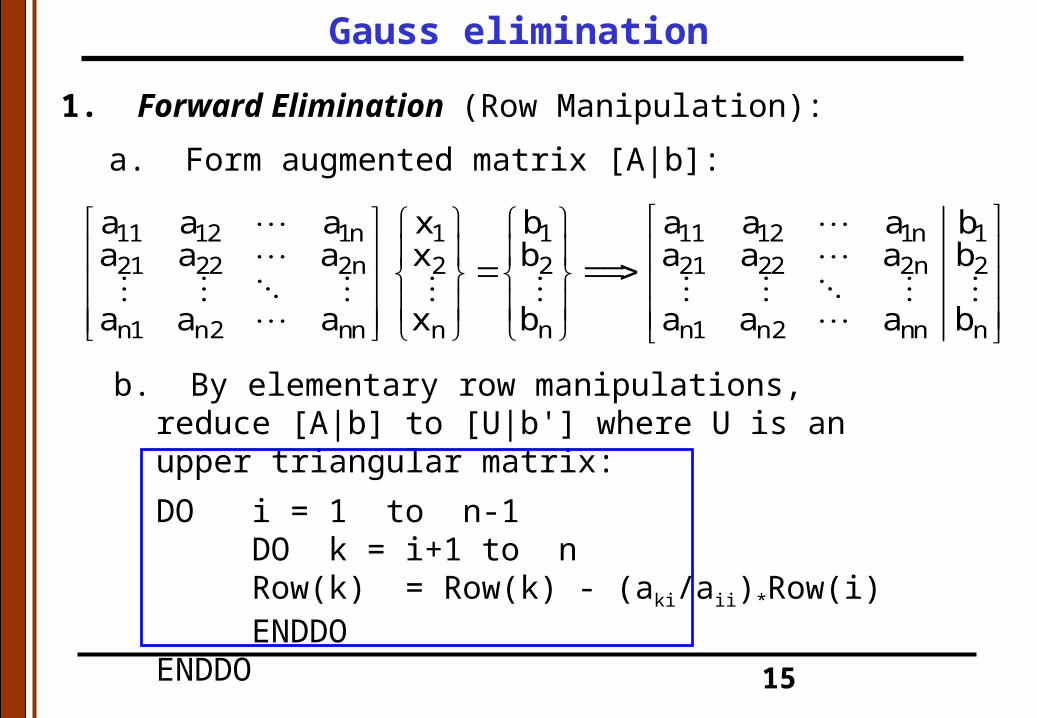
b. By elementary row manipulations, reduce [A|b] to [U|b'] where U is an upper triangular matrix:
DO i = 1 to n-1DO k = i+1 to nRow(k) = Row(k) - (aki/aii)*Row(i)ENDDO
ENDDO
11 12 1n 1 1 11 12 1n 121 22 2n 2 2 21 22 2n 2
n1 n2 nn n n n1 n2 nn n
a a a x b a a a ba a a x b a a a b
a a a x b a a a b
1. Forward Elimination (Row Manipulation):
a. Form augmented matrix [A|b]:
Gauss elimination

16
Gauss elimination
2. Back Substitution
Solve the upper triangular system [U]{x} = {b´}
xn = b'n / unn
DO i = n-1 to 1 by (-1)
END
n
i ij jj i 1
iii
b u x
xu
11 12 13 1n 1 1
22 23 2n 2 2
33 3n 3 3
nn n n
u u u u x b
0 u u u x b
0 0 u u x b
0 0 0 u x b
17
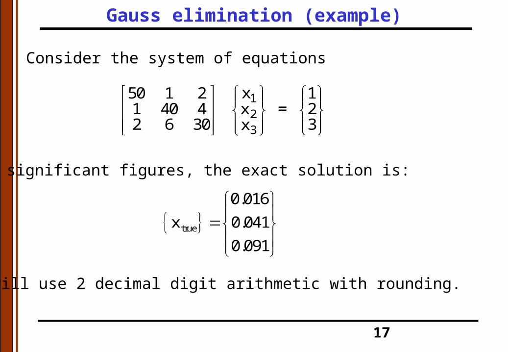
Consider the system of equations
123
x50 1 2 11 40 4 x = 22 6 30 3x
To 2 significant figures, the exact solution is:
true
0.016
x 0.041
0.091
We will use 2 decimal digit arithmetic with rounding.
Gauss elimination (example)
18
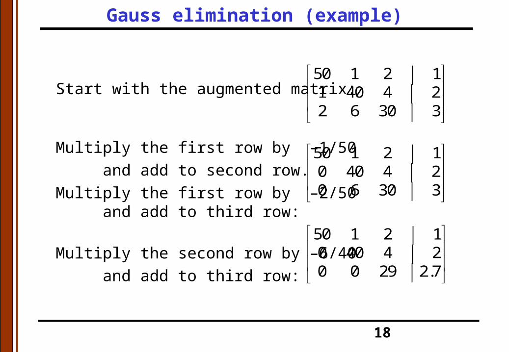
Start with the augmented matrix:
Multiply the first row by –1/50
and add to second row.
Multiply the first row by –2/50 and add to third row:
Multiply the second row by –6/40
and add to third row:
50 1 2 11 40 4 22 6 30 3
50 1 2 10 40 4 20 6 30 3
50 1 2 10 40 4 20 0 29 2.7
Gauss elimination (example)

19
Now backsolve:
50 1 2 10 40 4 20 0 29 2.7
32.7
x 0.09329
(vs. 0.091, t = 2.2%)
(vs. 0.041, t = 2.5%)
(vs. 0.016, t = 0%)
32
2 4xx 0.040
40
3 21
1 2x xx 0.016
50
Gauss elimination (example)
20
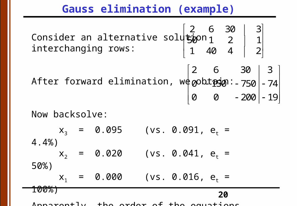
Consider an alternative solution interchanging rows:
After forward elimination, we obtain:
Now backsolve:
x3 = 0.095 (vs. 0.091, et = 4.4%)x2 = 0.020 (vs. 0.041, et = 50%)x1 = 0.000 (vs. 0.016, et = 100%)
Apparently, the order of the equations matters!
2 6 30 350 1 2 11 40 4 2
2 6 30 3
0 150 750 74
0 0 200 19
Gauss elimination (example)
21
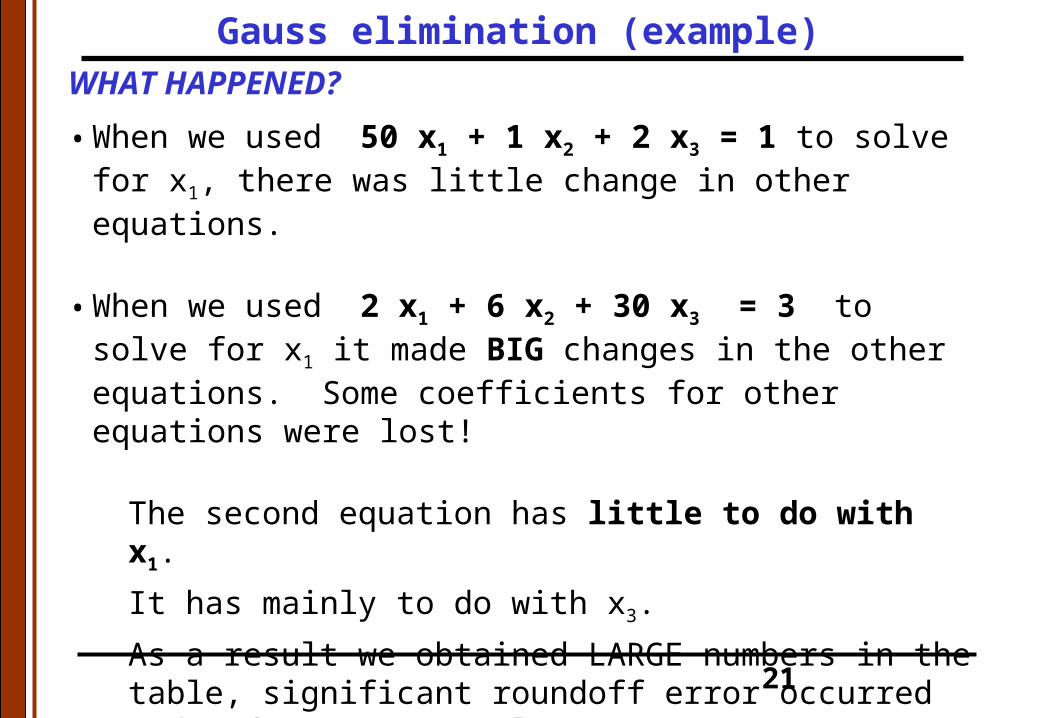
WHAT HAPPENED?
• When we used 50 x1 + 1 x2 + 2 x3 = 1 to solve for x1, there was little change in other equations.
• When we used 2 x1 + 6 x2 + 30 x3 = 3 to solve for x1 it made BIG changes in the other equations. Some coefficients for other equations were lost!
The second equation has little to do with x1.
It has mainly to do with x3.
As a result we obtained LARGE numbers in the table, significant roundoff error occurred and information was lost.
Things didn't go well!
• If scaling factors | aji / aii | are 1 then the effect of roundoff
errors is diminished.
Gauss elimination (example)

22
Effect of diagonal dominance:
As a first approximation roots are:
xi bi / aii
Consider the previous examples: true
0.016x = 0.041
0.091
123
50 1 2 1 x 1/50 =0.021 40 4 2 x 2/40 =0.05
x 3/30 =0.102 6 30 3
123
2 6 30 3 x 3/2 =1.550 1 2 1 x 1/1 =1.0
x 2/4 = 0.501 40 4 2
Gauss elimination (example)

23
Goals: 1. Best accuracy (i.e. minimize error)
2. Parsimony (i.e. minimize effort)
Possible Problems:A. Zero on diagonal term ÷ by zero.B. Many floating point operations (flops) cause numerical
precision problems and propagation of errors.C. System may be ill-conditioned: det[A] 0.D. No solution or an infinite # of solutions: det[A] = 0.
Possible Remedies:A. Carry more significant figures (double precision).B. Pivot when the diagonal is close to zero.C. Scale to reduce round-off error.
Gauss elimination (example)
24
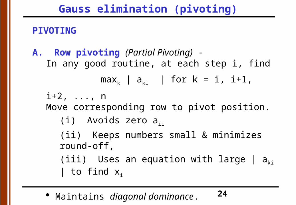
PIVOTING
A. Row pivoting (Partial Pivoting) - In any good routine, at each step i, find
maxk | aki | for k = i, i+1, i+2, ..., nMove corresponding row to pivot position.
(i) Avoids zero aii
(ii) Keeps numbers small & minimizes round-off,
(iii) Uses an equation with large | aki | to find xi
Maintains diagonal dominance. Row pivoting does not affect the order of the variables. Included in any good Gaussian Elimination routine.
Gauss elimination (pivoting)

25
B. Column pivoting - Reorder remaining variables xj
for j = i, . . . ,n so get largest | aji |Column pivoting changes the order of the unknowns, xi, and thus leads to complexity in the algorithm. Not usually done.
C. Complete or Full pivotingPerforming both row pivoting and column pivoting.(If [A] is symmetric, needed to preserve symmetry.)
Gauss elimination (pivoting)

26
How to fool pivoting:
Multiply the third equation by 100 and then performing pivoting will yield:
Forward elimination then yields (2-digit arithmetic):
Backsolution yields:
x3 = 0.095 (vs. 0.091, et = 4.4%)x2 = 0.020 (vs. 0.041, et = 50.0%)x1 = 0.000 (vs. 0.016, et = 100%)
The order of the rows is still poor!!
200 600 3000 300
50 1 2 1
1 40 4 2
200 600 3000 300
0 150 750 74
0 0 200 19
Gauss elimination (pivoting)
27
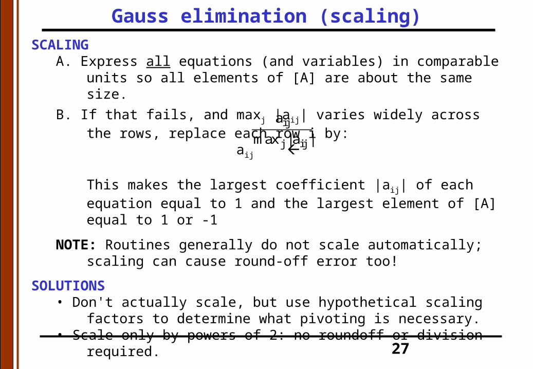
SCALINGA. Express all equations (and variables) in comparable units so all
elements of [A] are about the same size.
B. If that fails, and maxj |aij| varies widely across the rows, replace each row i by:
aij
This makes the largest coefficient |aij| of each equation equal to 1 and the largest element of [A] equal to 1 or -1
NOTE: Routines generally do not scale automatically; scaling can cause round-off error too!
SOLUTIONS • Don't actually scale, but use hypothetical scaling factors to determine
what pivoting is necessary.• Scale only by powers of 2: no roundoff or division required.
ij
j ij
a
max | a |
Gauss elimination (scaling)

28
If the units of x1 were expressed in µg instead of mg the matrix might read:
50 1 2 1
1 40 4 2
2 6 30 3
50000 1 2 1
1000 40 4 2
2000 6 3 3
1 0.00002 0.00001 0.00001
1 0.04 0.004 0.002
1 0.003 0.015 0.0015
How to fool scaling:A poor choice of units can undermine the value of scaling.
Begin with our original example:
Scaling then yields:
Which equation is used to determine x1 ? Why bother to scale ?
Gauss elimination (scaling)
29
OPERATION COUNTING
In numerical scientific calculations, the number of multiplies & divides often determines CPU time. (This represents the numerical effort!)
One floating point multiply or divide (plus any associated adds or subtracts) is called a FLOP. (The adds/subtracts use little time compared to the multiplies/divides.) FLOP = FLoating point OPeration.
Examples: a * x + b a / x – b
Gauss elimination (operation counting)
30
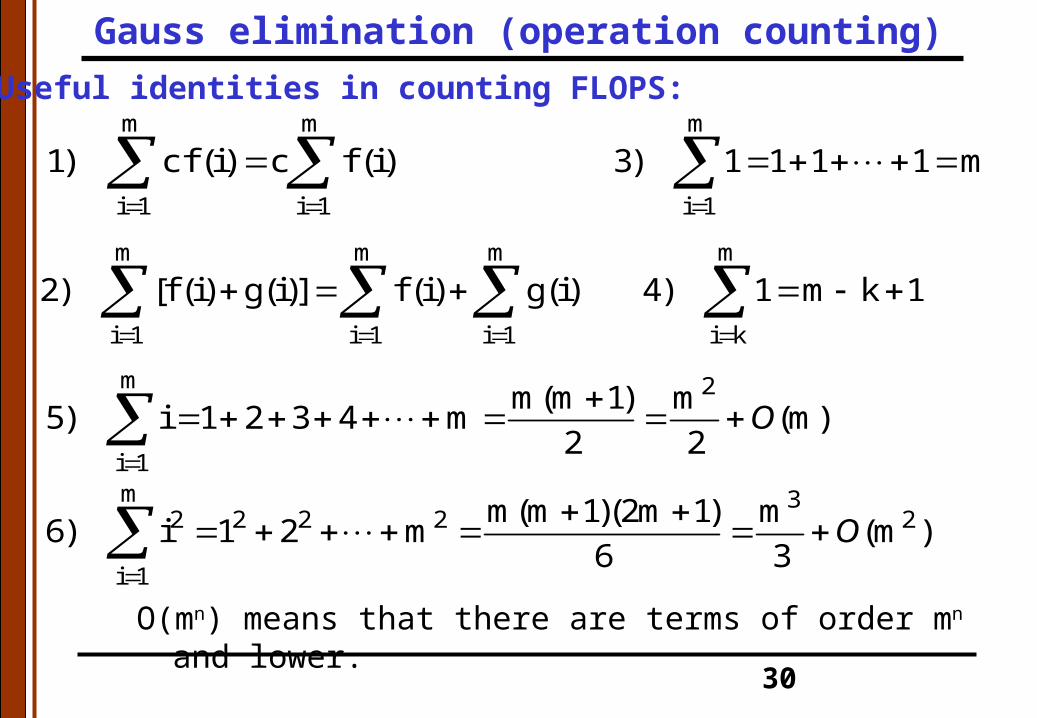
Useful identities in counting FLOPS:m m
i 1 i 1
1) c f (i) c f (i)
m m m
i 1 i 1 i 1
2) [f (i) g(i)] f (i) g(i)
m
i 1
3) 1 1 1 1 m
m
i k
4) 1 m k 1
m 2
i 1
m(m 1) m5) i 1 2 3 4 m (m)
2 2
O
m 32 2 2 2 2
i 1
m(m 1)(2m 1) m6) i 1 2 m (m )
6 3
O
O(mn) means that there are terms of order mn and lower.
Gauss elimination (operation counting)
31
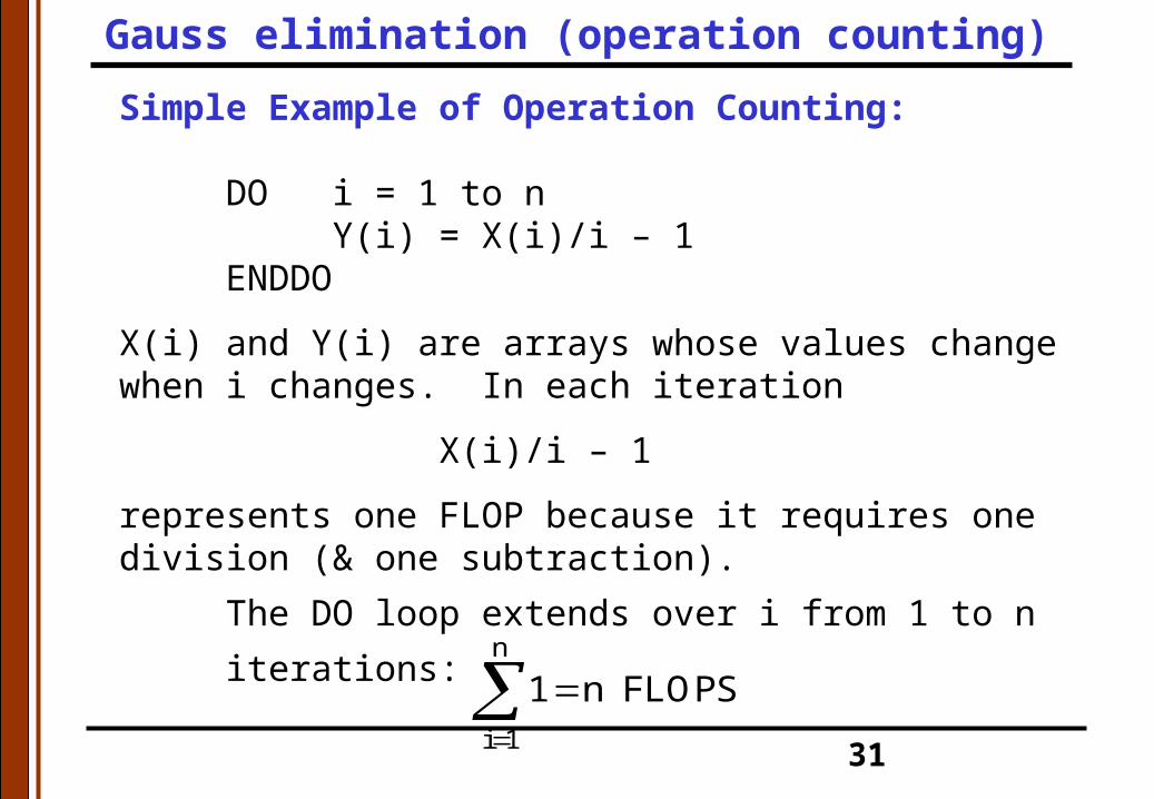
Simple Example of Operation Counting:
DO i = 1 to nY(i) = X(i)/i – 1
ENDDO
X(i) and Y(i) are arrays whose values change when i changes. In each iteration
X(i)/i – 1
represents one FLOP because it requires one division (& one subtraction).
The DO loop extends over i from 1 to n iterations:n
i 1
1 n FLOPS
Gauss elimination (operation counting)
32
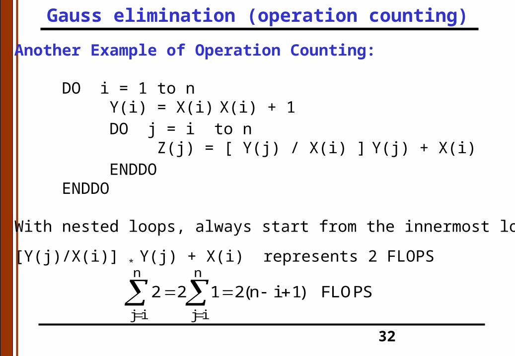
Another Example of Operation Counting:
DO i = 1 to nY(i) = X(i) X(i) + 1DO j = i to n
Z(j) = [ Y(j) / X(i) ] Y(j) + X(i)ENDDO
ENDDO
With nested loops, always start from the innermost loop.
[Y(j)/X(i)] * Y(j) + X(i) represents 2 FLOPSn n
j i j i
2 2 1 2(n i 1) FLOPS
Gauss elimination (operation counting)

33
For the outer i-loop: X(i) • X(i) + 1 represents 1 FLOP
n n n
i 1 i 1 i 1
1 2 n i 1) 3 2n 1 2 i
n(n 1)3 2n n 2
2
= 3n +2n2 - n2 - n
= n2 + 2n = n2 + O(n)
Gauss elimination (operation counting)

34
Forward Elimination:DO k = 1 to n–1
DO i = k+1 to nr = A(i,k)/A(k,k)
DO j = k+1 to n A(i,j)=A(i,j) – r*A(k,j)ENDDO
B(i) = B(i) – r*B(k)ENDDO
ENDDO
Gauss elimination (operation counting)
35
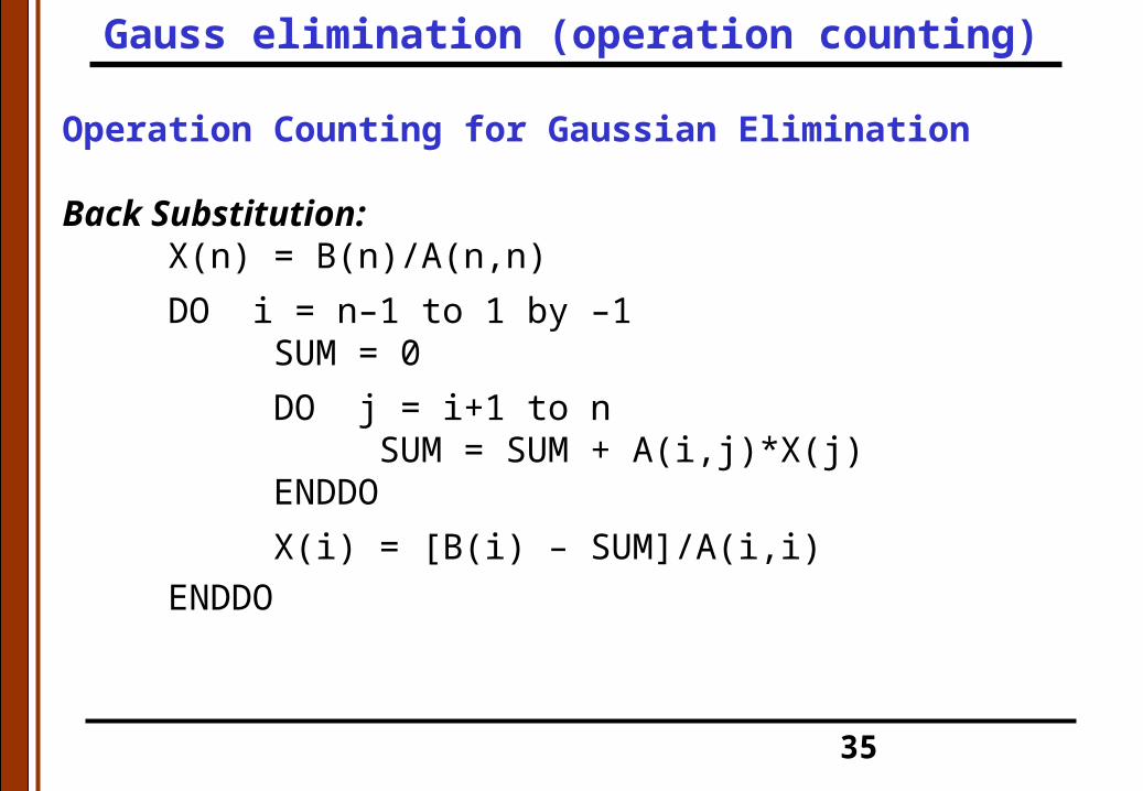
Operation Counting for Gaussian Elimination
Back Substitution:X(n) = B(n)/A(n,n)
DO i = n–1 to 1 by –1SUM = 0
DO j = i+1 to nSUM = SUM + A(i,j)*X(j)
ENDDO
X(i) = [B(i) – SUM]/A(i,i)
ENDDO
Gauss elimination (operation counting)
36
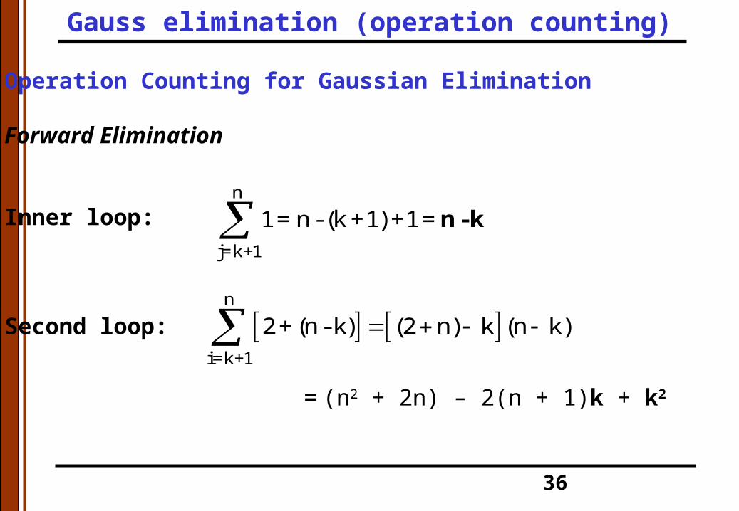
Operation Counting for Gaussian Elimination
Forward Elimination
Inner loop:
Second loop:
n
j=k+1
1 = n - (k +1) +1 = n - k
n
i=k+1
2 + (n - k) (2 n) k (n k) = (n2 + 2n) – 2(n + 1)k + k2
Gauss elimination (operation counting)
37
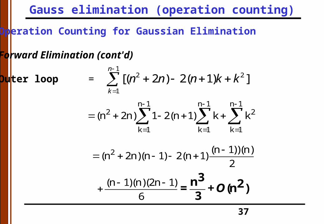
Operation Counting for Gaussian Elimination
Forward Elimination (cont'd)
Outer loop =1
2 2
1
[( 2 ) 2( 1) ]n
k
n n n k k
n 1 n 1 n 1
2 2
k 1 k 1 k 1
(n 2n) 1 2(n 1) k k
2 (n 1))(n)(n 2n)(n 1) 2(n 1)
2
(n 1)(n)(2n 1)
6
3n 2= + (n )3
O
Gauss elimination (operation counting)
38
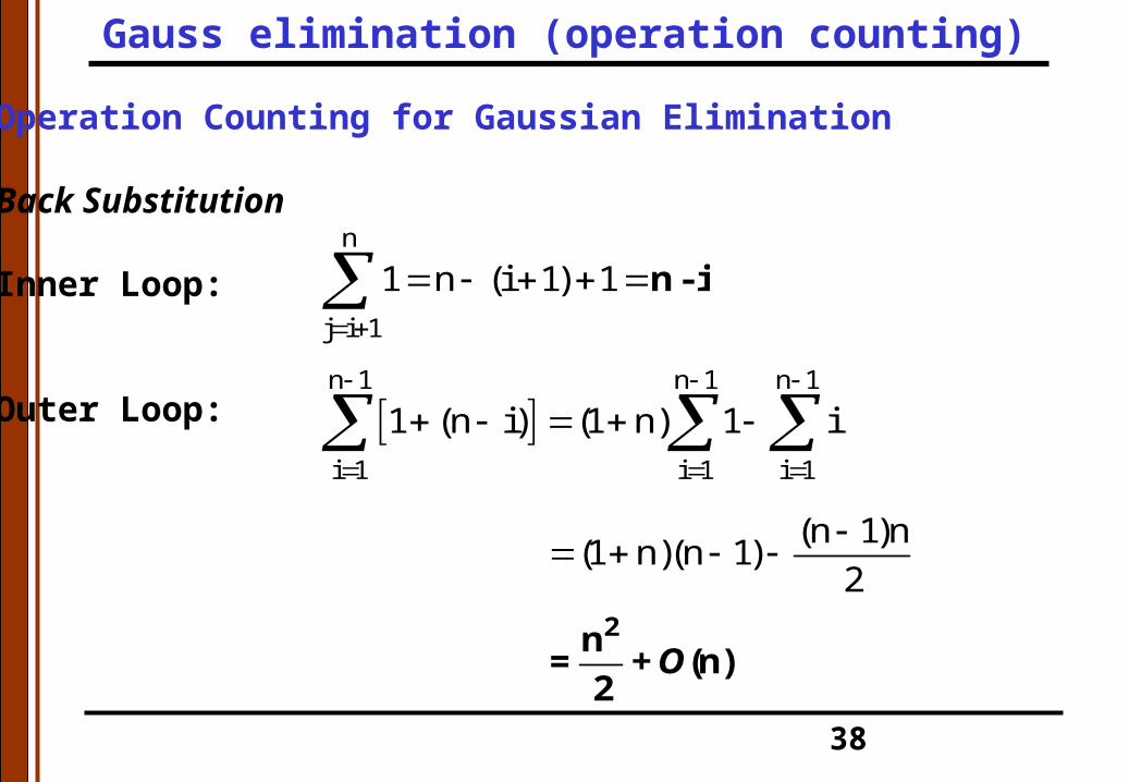
Operation Counting for Gaussian Elimination
Back Substitution
Inner Loop:
Outer Loop:
n
j i 1
1 n (i 1) 1
n - i
n 1 n 1 n 1
i 1 i 1 i 1
1 (n i) (1 n) 1 i
(n 1)n
(1 n)(n 1)2
2n= + (n)
2O
Gauss elimination (operation counting)
39
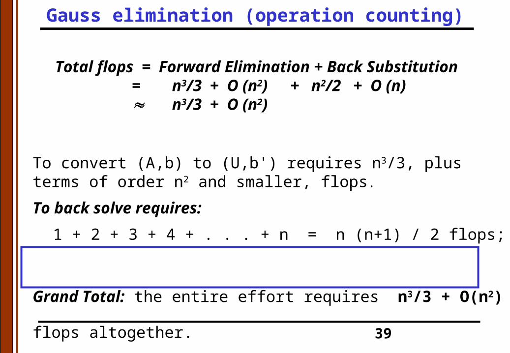
Total flops = Forward Elimination + Back Substitution= n3/3 + O (n2) + n2/2 + O (n) n3/3 + O (n2)
To convert (A,b) to (U,b') requires n3/3, plus terms of order n2 and smaller, flops.
To back solve requires:
1 + 2 + 3 + 4 + . . . + n = n (n+1) / 2 flops;
Grand Total: the entire effort requires n3/3 + O(n2) flops altogether.
Gauss elimination (operation counting)

40
Diagonalization by both forward and backward elimination in each column.
Perform elimination both backwards and forwards until:
Operation count for Gauss-Jordan is: (slower than Gauss elimination)
11 12 13 1n 1 1
21 22 23 2n 2 2
31 32 33 3n 3 3
n1 n2 n3 nn nn n
a a a ... a x b
a a a ... a x b
=a a a ... a x b
...
a a a ... a x b
1 1
2 2
3 3
n n
x x1 0 0 0
x x0 1 0 0
= x x0 0 1 0
x x0 0 0 1
32n
O(n )2
Gauss-Jordan Elimination
41
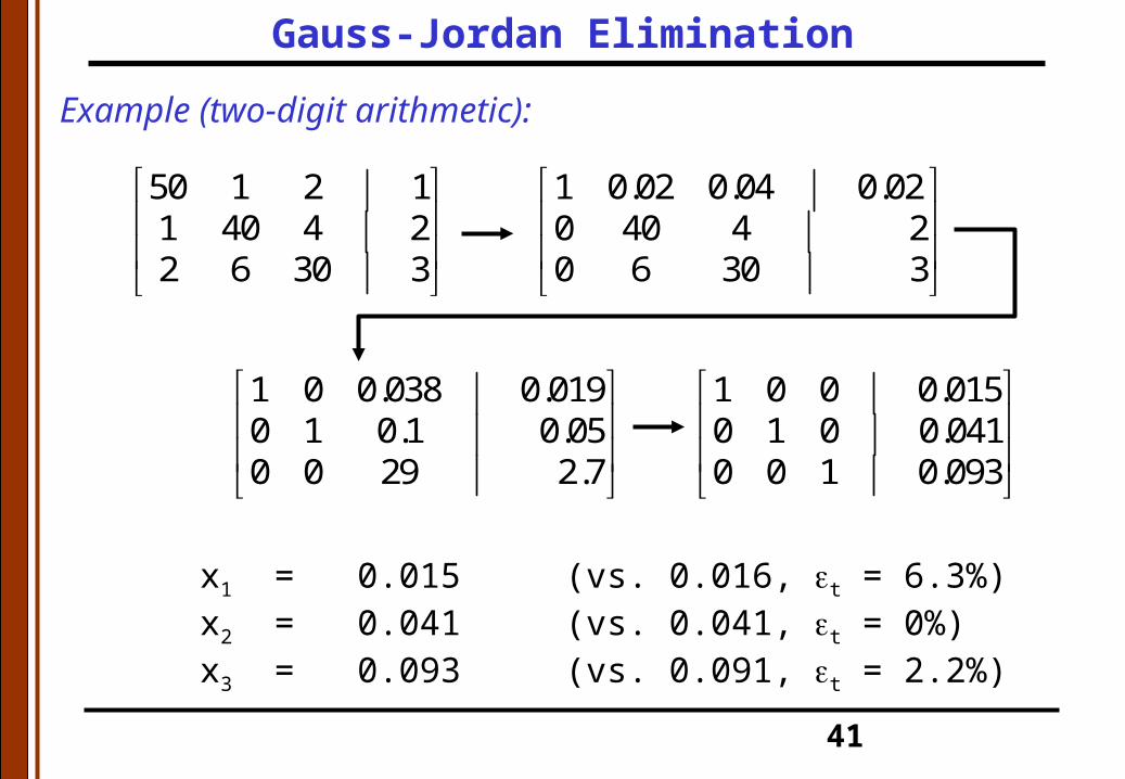
Example (two-digit arithmetic):
50 1 2 11 40 4 22 6 30 3
1 0.02 0.04 0.020 40 4 20 6 30 3
1 0 0.038 0.0190 1 0.1 0.050 0 29 2.7
1 0 0 0.0150 1 0 0.0410 0 1 0.093
x1 = 0.015 (vs. 0.016, t = 6.3%)x2 = 0.041 (vs. 0.041, t = 0%)x3 = 0.093 (vs. 0.091, t = 2.2%)
Gauss-Jordan Elimination

42
The solution of: [A]{x} = {b} is: {x} = [A]-1{b}
where [A]-1 is the inverse matrix of [A]
Consider: [A] [A]-1 = [ I ]
1) Create the augmented matrix: [ A | I ]
2) Apply Gauss-Jordan elimination:
==> [ I | A-1 ]
Gauss-Jordan Matrix Inversion

43
Gauss-Jordan Matrix Inversion (with 2 digit arithmetic):
50 1 2 1 0 0A I = 1 40 4 0 1 0
2 6 30 0 0 1
1 0.02 0.04 0.02 0 00 40 4 -0.02 1 00 6 30 -0.04 0 1
MATRIX INVERSE [A-1]
1 0 0 0.02 0.00029 0.0014
0 1 0 0.00037 0.026 0.0036
0 0 1 0.0013 0.0054 0.036
1 0 0.038 0.02 0.005 0
0 1 0.1 0.0005 0.025 0
0 0 28 0.037 0.15 1
Gauss-Jordan Matrix Inversion

44
50 1 2 0.020 -0.00029 -0.0014 0.997 0.13 0.0022 40 4 -0.00037 0.026 -0.0036 0.000 1.016 0.0012 6 30 -0.0013 -0.0054 0.036 0.001 0.012 1.056
CHECK:[ A ] [ A ]-1 = [ I ]
[ A ]-1 { b } = { x }
0.020 -0.0029 -0.0014 1 0.015-0.00037 0.026 -0.0036 2 0.033-0.0013 -0.0054 0.036 3 0.099
true
0.016x 0.041
0.091
0.016x 0.040
0.093
GaussianElimination
Gauss-Jordan Matrix Inversion
45
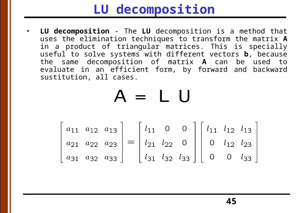
LU decomposition
• LU decomposition - The LU decomposition is a method that uses the elimination techniques to transform the matrix A in a product of triangular matrices. This is specially useful to solve systems with different vectors b, because the same decomposition of matrix A can be used to evaluate in an efficient form, by forward and backward sustitution, all cases.

46
LU decomposition
Decomposition Initial system
Transformed system 1Substitution
Transformed system 2
Forward sustitutionBackward sustitution
47
LU decomposition
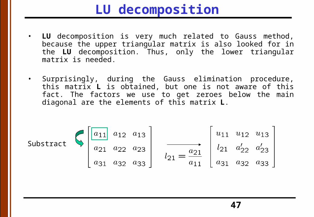
• LU decomposition is very much related to Gauss method, because the upper triangular matrix is also looked for in the LU decomposition. Thus, only the lower triangular matrix is needed.
• Surprisingly, during the Gauss elimination procedure, this matrix L is obtained, but one is not aware of this fact. The factors we use to get zeroes below the main diagonal are the elements of this matrix L.
Substract

48
LU decomposition
resto
resto

49
Basic Approach
Consider [A]{x} = {b}
a) Gauss-type "decomposition" of [A] into [L][U] n3/3 flops [A]{x} = {b} becomes [L] [U]{x} = {b}; let [U]{x} {d}
b) First solve [L] {d} = {b} for {d} by forward subst. n2/2 flops
c) Then solve [U]{x} = {d} for {x} by back substitution n2/2 flops
LU decomposition (Complexity)
50
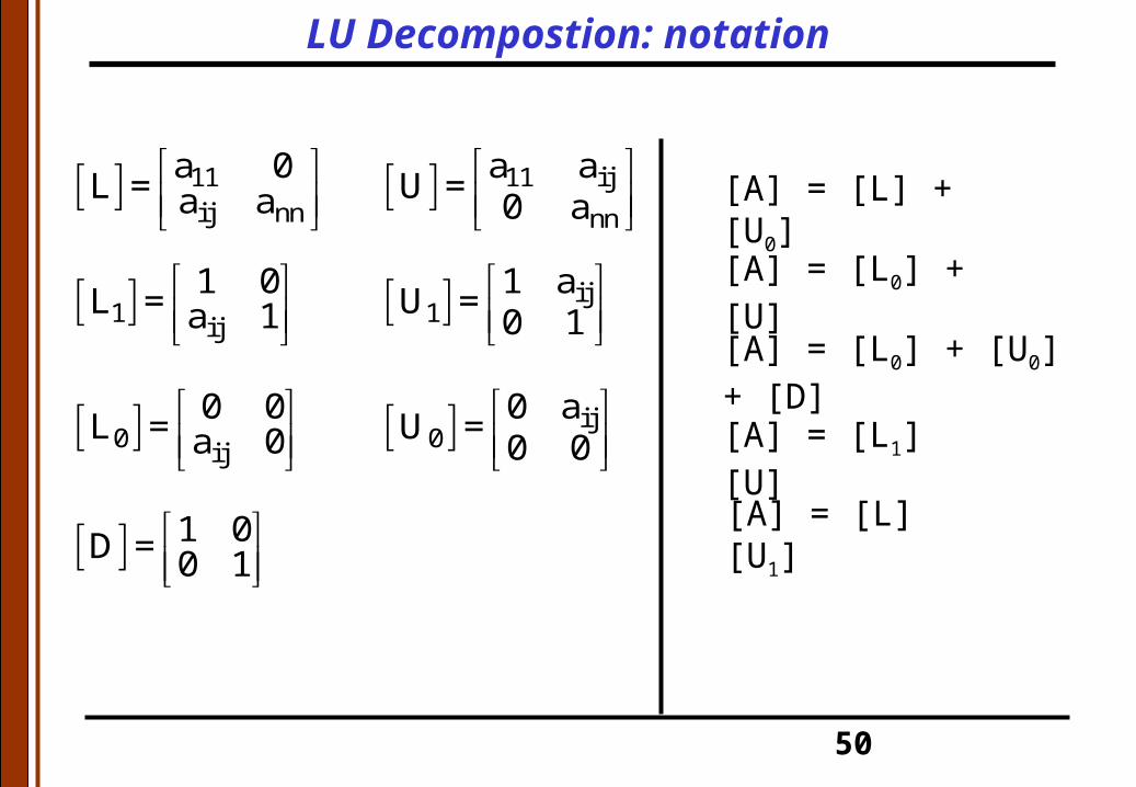
1ij
1 0L = a 1
0ij
0 0L = a 0
ij0
0 aU =
0 0
ij1
1 aU =
0 1
1 0D = 0 1
[A] = [L] + [U0]
[A] = [L0] + [U]
[A] = [L0] + [U0] + [D]
11ij nn
a 0L = a a
11 ij
nn
a aU =
0 a
[A] = [L1] [U]
[A] = [L] [U1]
LU Decompostion: notation

51
LU Decomposition VariationsDoolittle [L1][U] General [A]Crout [L][U1] General [A]Cholesky[L][L] T Pos. Def. Symmetric [A]
Cholesky works only for Positive Definite Symmetric matrices
Doolittle versus Crout:• Doolittle just stores Gaussian elimination factors where Crout
uses a different series of calculations (see C&C 10.1.4).• Both decompose [A] into [L] and [U] in n3/3 FLOPS
• Different location of diagonal of 1's• Crout uses each element of [A] only once so the same array
can be used for [A] and [L\U] saving computer memory!
LU decomposition

52
Matrix Inversion
Definition of a matrix inverse:
[A] [A]-1 = [ I ]
==> [A] {x} = {b}
[A]-1 {b} = {x}
First Rule: Don’t do it.
(numerically unstable calculation)
LU decomposition
53
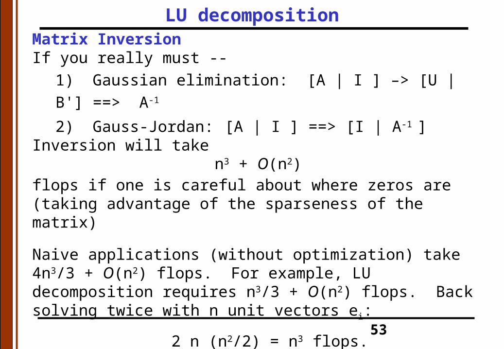
Matrix InversionIf you really must --
1) Gaussian elimination: [A | I ] –> [U | B'] ==> A-1
2) Gauss-Jordan: [A | I ] ==> [I | A-1 ] Inversion will take
n3 + O(n2)flops if one is careful about where zeros are (taking advantage of the sparseness of the matrix)
Naive applications (without optimization) take 4n3/3 + O(n2) flops. For example, LU decomposition requires n3/3 + O(n2) flops. Back solving twice with n unit vectors ei:
2 n (n2/2) = n3 flops.
Altogether: n3/3 + n3 = 4n3/3 + O(n2) flops
LU decomposition