N95- 10568

Characteristics of a Dry, Pulsating

Microburst at Denver Stapleton Airport.

E Proctor,

NASA Langley Research Center

[For these Proceedings, the author has furnished three papers:

Influence of Low-Level Environmental Shear on Microburst Structure:

Numerical Case Study,

Numerical Simulation of a Pulsating, Low-Reflectivity Microburst Event,

and

Case Study of a Low-Reflectivity Pulsating Microburst: Numerical Simulation of

the Denver, 8 July 1989, Storm.

These appear in order on the following pages.]

177

https://ntrs.nasa.gov/search.jsp?R=19950004156 2018-06-25T02:54:13+00:00Z

1,1.1

m

oiZWZ_0

i-

ra

0_10Z

0w_

w

w__ I,i,I

Z_

w_Zm

00

I-ra

/

178

I

.o

Z

179

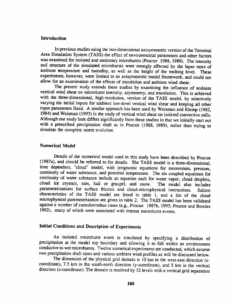
Introduction

In previous studies using the two-dimensional axisymmetric version of the Terminal

Area Simulation System (TASS) the effect of environmental parameters and other factors

was examined for isolated and stationary microbursts (Proctor 1988, 1989). The intensity

and structure of the simulated microbursts were strongly affected by the lapse rates of

ambient temperature and humidity, as well as the height of the melting level. These

experiments, however, were limited to an axisymmetric model framework, and could not

allow for an examination of the effects of translation and ambient wind shear.

The present study extends these studies by examining the influence of ambient

vertical wind shear on microburst intensity, asymmetry, and translation. This is achieved

with the three-dimensional, high-resolution, version of the TASS model, by selectively

varying the initial inputs for ambient low-level vertical wind shear and keeping all other

input parameters fLxed. A similar approach has been used by Weisman and Klemp (1982,

1984) and Weisman (1993) in the study of vertical wind shear on isolated convective cells.

Although our study here differs significantly from these studies in that we initially start out

with a prescribed precipitation shaft as in Proctor (1988, 1989), rather than trying to

simulate the complete storm evolution.

Numerical Model

Details of the numerical model used in this study have been described by Proctor

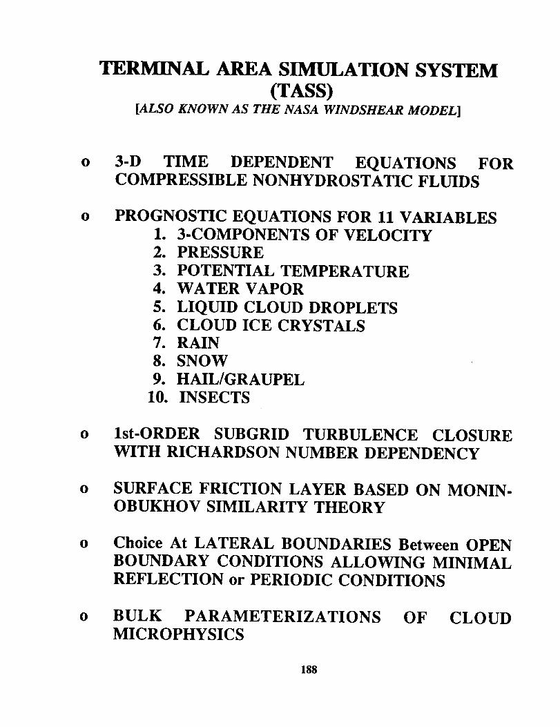
(1987a), and should be referred to for details. The TASS model is a three-dimensional,

time dependent, "cloud" model, with prognostic equations for momentum, pressure,

continuity of water substance, and potential temperature. The six coupled equations for

continuity of water substance include an equation each for water vapor, cloud droplets,

cloud ice crystals, rain, hail or graupel, and snow. The model also includes

parameterizations for surface friction and cloud-microphysical interactions. Salientcharacteristics of the TASS model are listed in table 1, and a list of the cloud

microphysical parameterization are given in table 2. The TASS model has been validated

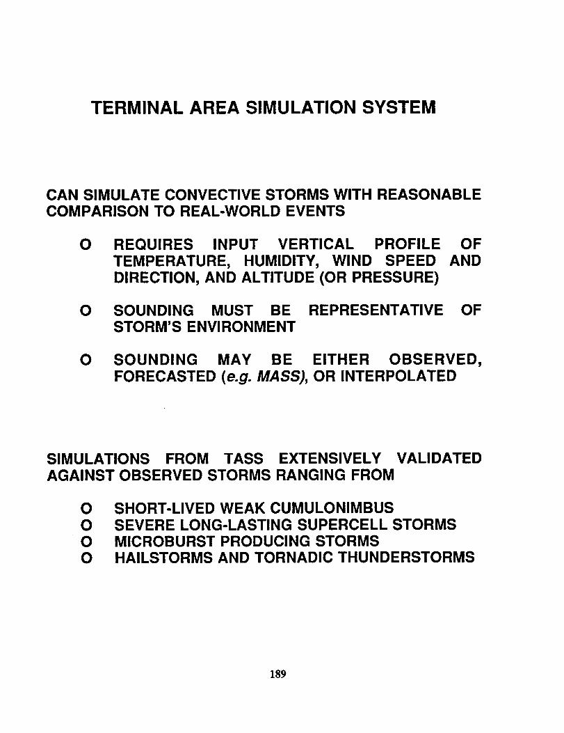
against a number of cumulonimbus cases (e.g., Proctor 1987b, 1993; Proctor and Bowles

1992), many of which were associated with intense microburst events.

Initial Conditions and Description of Experiments

An isolated microburst event is simulated by specifying a distribution of

precipitation at the model top boundary and allowing it to fall within an environment

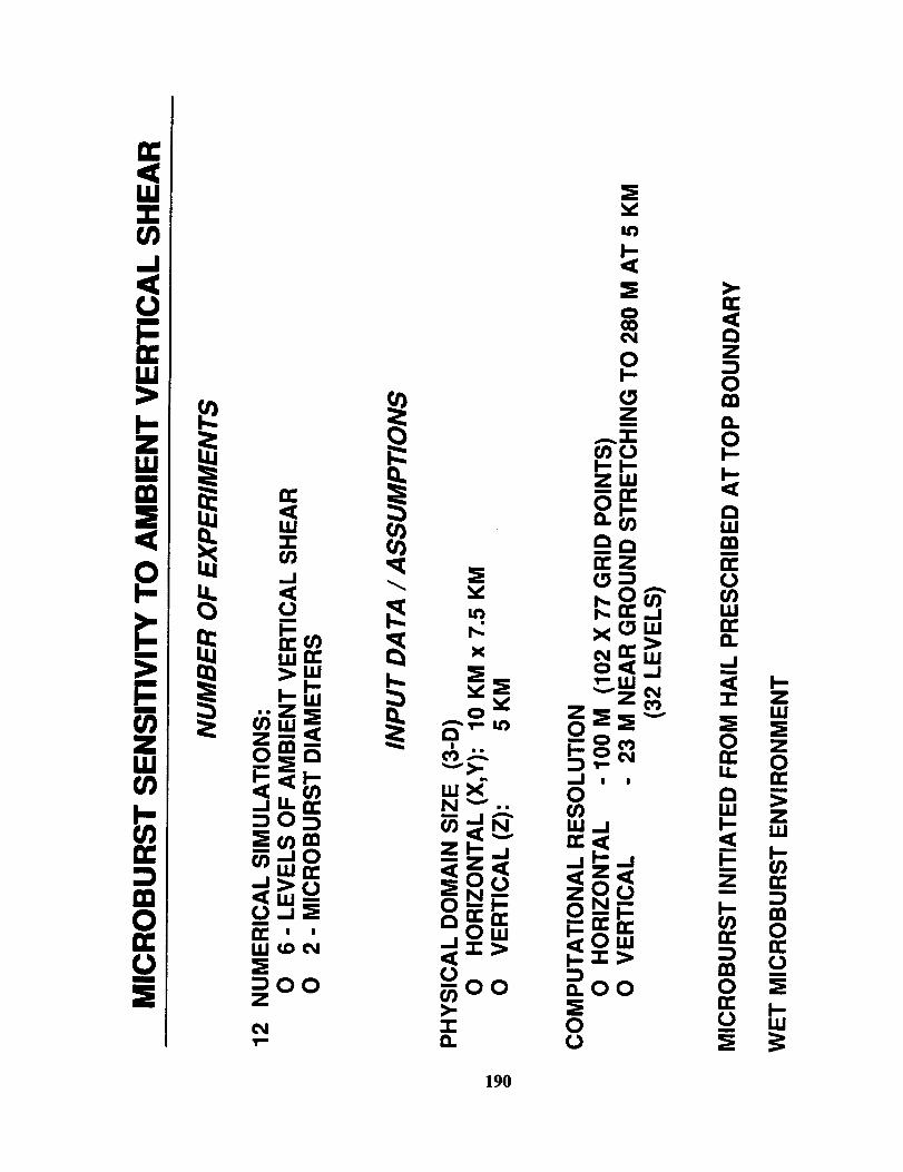
conducive to wet microbursts. Twelve numerical experiments are conducted, which assume

two precipitation shaft sizes and various ambient wind profiles as will be discussed below.

The dimension of the physical grid domain is 10 km in the west-east direction (x-

coordinate), 7.5 km in the south-north direction (y-coordinate), and 5 km in the vertical

direction (z-coordinate). The domain is resolved by 32 levels with a vertical grid separation

180

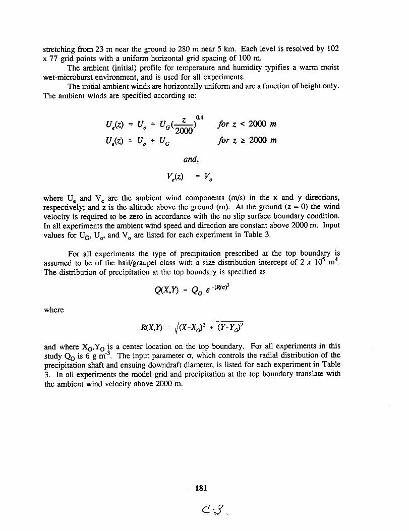
stretching from 23 m near the ground to 280 m near 5 km. Each level is resolved by 102

x 77 grid points with a uniform horizontal grid spacing of 100 m.

The ambient (initial) profile for temperature and humidity typifies a warm moist

wet-microburst environment, and is used for all experiments.

The initial ambient winds are horizontally uniform and are a function of height only.

The ambient winds are specified according to:

Z 0.4

U,(z)-- Vo + U (T-U,fz)--Uo +Uo

for z < 2000 m

for z > 2000 m

and,

V,<z) -- vo

where U e and V e are the ambient wind components (m/s) in the x and y directions,

respectively; and z is the altitude above the ground (m). At the ground (z = 0) the wind

velocity is required to be zero in accordance with the no slip surface boundary condition.

In all experiments the ambient wind speed and direction are constant above 2000 m. Input

values for U G, U o, and V o are listed for each experiment in Table 3.

For all experiments the type of precipitation prescribed at the top boundary isassumed to be of the hail/graupel class with a size distribution intercept of 2 x 105 m 4.

The distribution of precipitation at the top boundary is specified as

Q(X,Y) = Qo e-(R/°)3

where

g(x,r) : ¢(x-xo)2 ÷ (r-roY

and where Xo,Y o is a center location on the top boundary. For all experiments in this

study Qo is 6 g m -3. The input parameter c, which controls the radial distribution of the

precipitation shaft and ensuing downdraft diameter, is listed for each experiment in Table

3. In all experiments the model grid and precipitation at the top boundary translate with

the ambient wind velocity above 2000 m.

181

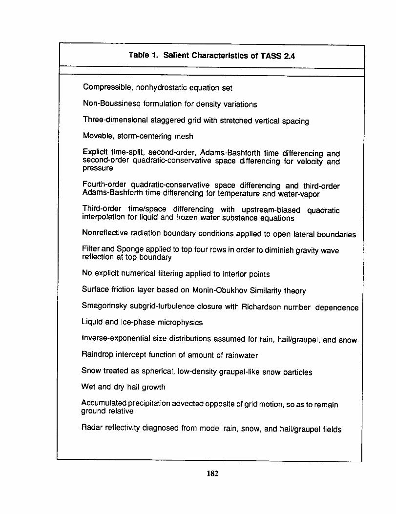
Table 1. Salient Characteristics of TASS 2.4

Compressible, nonhydrostatic equation set

Non-Boussinesq formulation for density variations

Three-dimensional staggered grid with stretched vertical spacing

Movable, storm-centering mesh

Explicit time-split, second-order, Adams-Bashforth time differencing andsecond-order quadratic-conservative space differencing for velocity andpressure

Fourth-order quadratic-conservative space differencing and third-orderAdams-Bashforth time differencing for temperature and water-vapor

Third-order time/space differencing with upstream-biased quadraticinterpolation for liquid and frozen water substance equations

Nonreflective radiation boundary conditions applied to open lateral boundaries

Filter and Sponge applied to top four rows in order to diminish gravity wavereflection at top boundary

No explicit numerical filtering applied to interior points

Surface friction layer based on Monin-Obukhov Similarity theory

Smagorinsky subgrid-turbulence closure with Richardson number dependence

Liquid and ice-phase microphysics

Inverse-exponential size distributions assumed for rain, hail/graupel, and snow

Raindrop intercept function of amount of rainwater

Snow treated as spherical, low-density graupel-like snow particles

Wet and dry hail growth

Accumulated precipitation advected opposite of grid motion, so as to remainground relative

Radar reflectivity diagnosed from model rain, snow, and hail/graupel fields

182

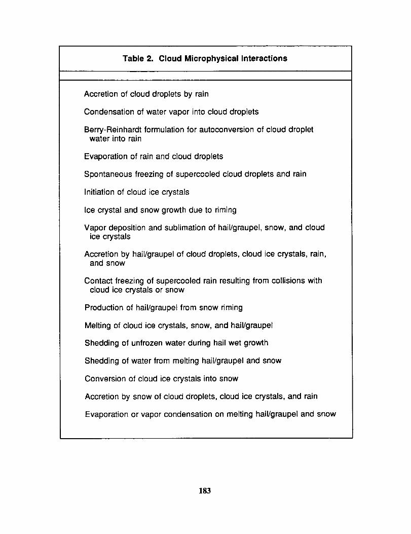
Table 2. Cloud Microphysical Interactions

Accretion of cloud droplets by rain

Condensation of water vapor into cloud droplets

Berry-Reinhardt formulation for autoconversion of cloud dropletwater into rain

Evaporation of rain and cloud droplets

Spontaneous freezing of supercooled cloud droplets and rain

Initiation of cloud ice crystals

Ice crystal and snow growth due to riming

Vapor deposition and sublimation of hail/graupel, snow, and cloudice crystals

Accretion by hail/graupel of cloud droplets, cloud ice crystals, rain,and snow

Contact freezing of supercooled rain resulting from collisions withcloud ice crystals or snow

Production of hail/graupel from snow riming

Melting of cloud ice crystals, snow, and hail/graupel

Shedding of unfrozen water during hail wet growth

Shedding of water from melting hail/graupel and snow

Conversion of cloud ice crystals into snow

Accretion by snow of cloud droplets, cloud ice crystals, and rain

Evaporation or vapor condensation on melting hail/graupel and snow

183

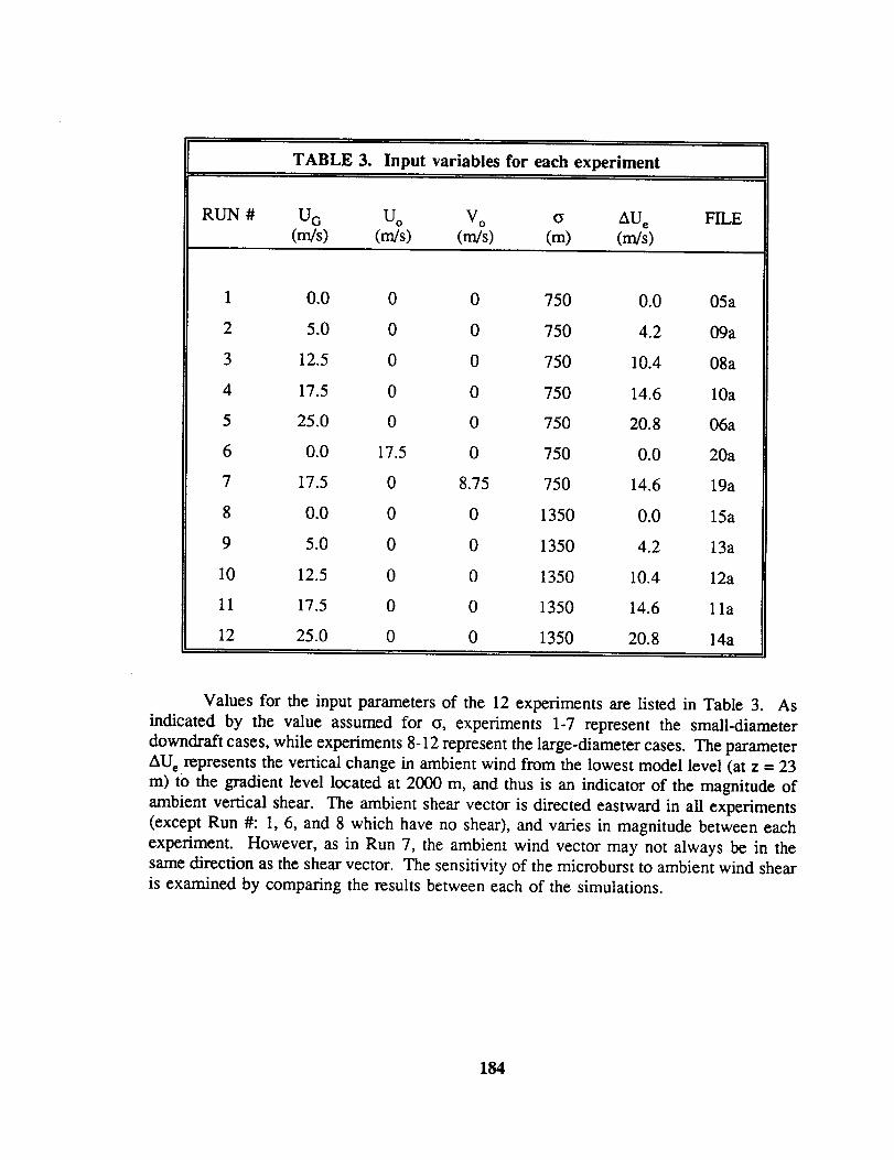
TABLE 3. Input variables for each experiment

RUN # U G U o V ° o AU e FILE

(m/s) (m/s) (m/s) (m) (m/s)

1 0.0 0 0 750 0.0 05a

2 5.0 0 0 750 4.2 09a

3 12.5 0 0 750 10.4 08a

4 17.5 0 0 750 14.6 10a

5 25.0 0 0 750 20.8 06a

6 0.0 17.5 0 750 0.0 20a

7 17.5 0 8.75 750 14.6 19a

8 0.0 0 0 1350 0.0 15a

9 5.0 0 0 1350 4.2 13a

10 12.5 0 0 1350 10.4 12a

11 17.5 0 0 1350 14.6 lla

12 25.0 0 0 1350 20.8 14a

Values for the input parameters of the 12 experiments are listed in Table 3. As

indicated by the value assumed for o, experiments 1-7 represent the small-diameter

downdraft cases, while experiments 8-12 represent the large-diameter cases. The parameter

AU e represents the vertical change in ambient wind from the lowest model level (at z - 23

m) tO the gradient level located at 2000 m, and thus is an indicator of the magnitude of

ambient vertical shear. The ambient shear vector is directed eastward in all experiments

(except Run #: 1, 6, and 8 which have no shear), and varies in magnitude between each

experiment. However, as in Run 7, the ambient wind vector may not always be in the

same direction as the shear vector. The sensitivity of the microburst to ambient wind shear

is examined by comparing the results between each of the simulations.

184

Results

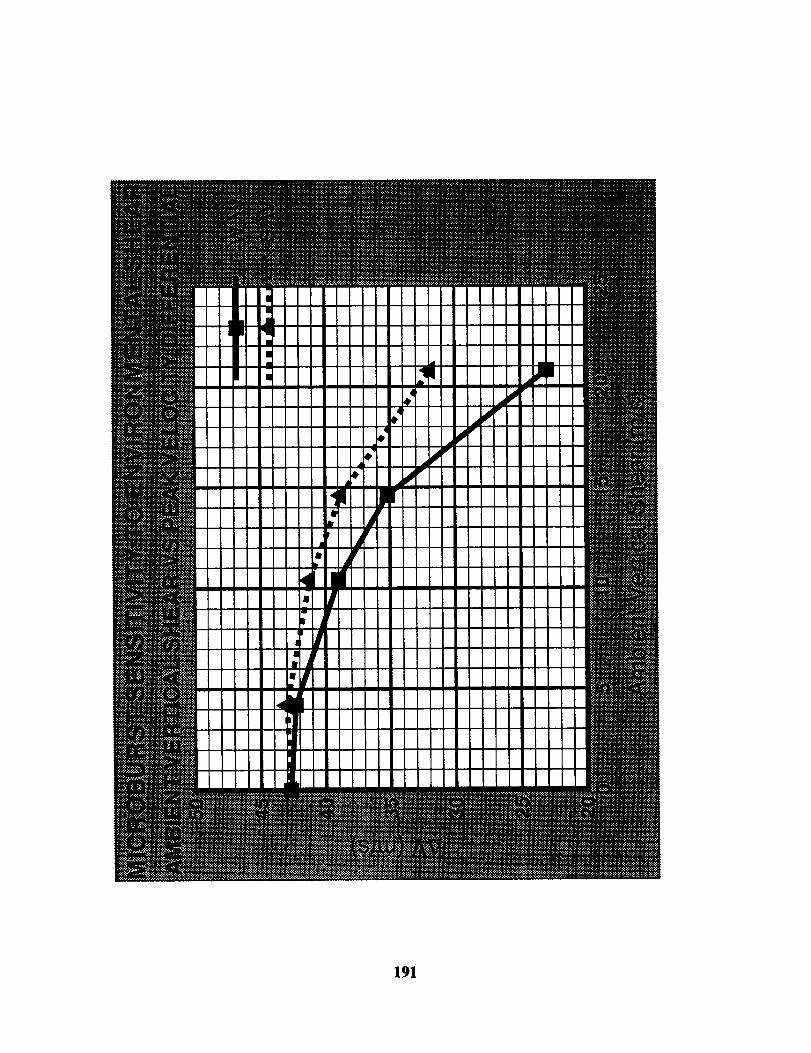
Sensitivity of key microburst parameters to environmental shear are shown in the

following three line plots. The tendencies of both the small and large diameter rnicroburst

were similar and thus only results from the small diameter microburst are shown in the first

two plots.

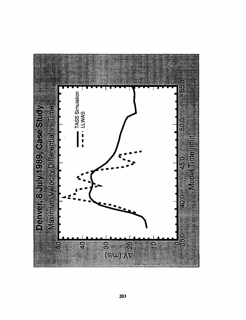
The plot of ambient vertical shear vs peak velocity differential shows that increasing

ambient shear reduces the peak velocity differential of a microburst. More importantly

though, the peak velocity differential that is orthogonal to the ambient shear vector (e.g.

AV along north-south segments) are less affected by increasing shear than the velocity

differential along the shear vector (e.g. AV along east-west segments). Asymmetry of the

microburst outflow field is indicated the by the difference in magnitude between the E-W

and N-S segments. [For an axisymmetric outflow the peak E-W AV is equal to the peak

N-S AV.] The results show that asymmetry of the outflow velocity field increases with

increasing ambient shear.

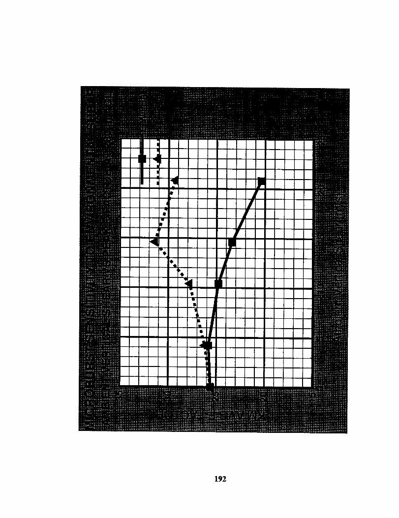
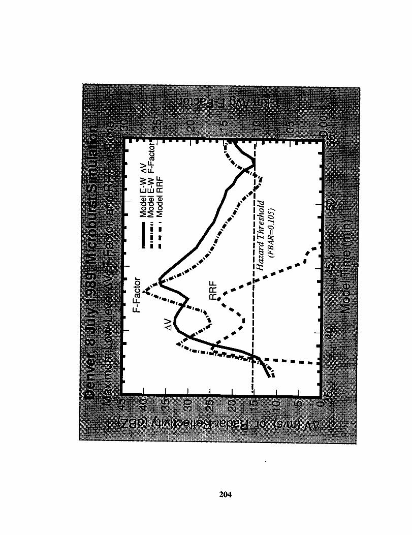
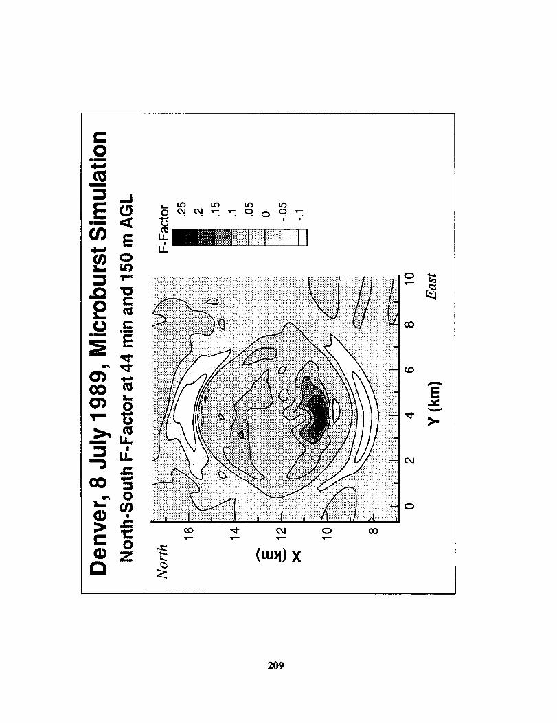
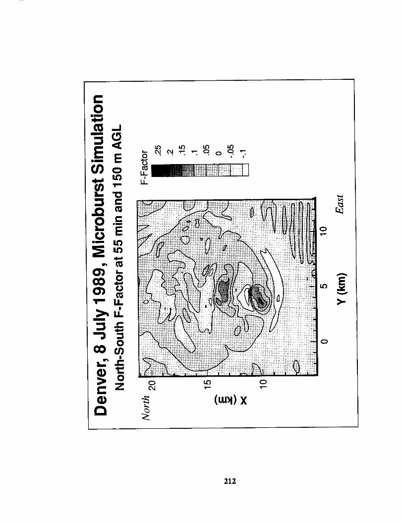
The second line plot shows the sensitivity of peak Fbar (1-km averaged F-Factor)

at 280 m AGL. As described in Proctor and Bowles (1992) and Switzer et al (1993),

values for F-factor are computed assuming horizontal north-south (or east-west) trajectories

with an assumed air speed of 75 m/s. Similar to the peak AV curves in the previous plot,

peak Fbar along segments orthogonal to the shear vector are stronger than the peak values

along segments parallel to the shear vector, with widening differences as the magnitude of

shear increases. But unlike in the previous plot, an optimal value occurs for Fbar along

segments orthogonal to the shear vector. This optimal value happens for the north-south

Fbar when the magnitude of the ambient shear is approximately 15 m/s.

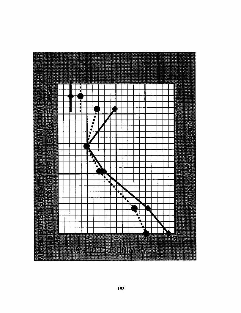
The third plot show the sensitivity of peak outflow speed (ground relative) for both

large and small diameter microbursts. The peak outflow speed indicates the severity of

the microburst in terms of its potential for inducing damage due to high winds. Our set

of experiments indicates that the highest wind speeds occur for an optimal ambient vertical

shear of about 15 m/s for both large and small diameter microbursts. The simulations

indicate that this peak horizontal wind speed occurs on the downshear side of themicrobursts.

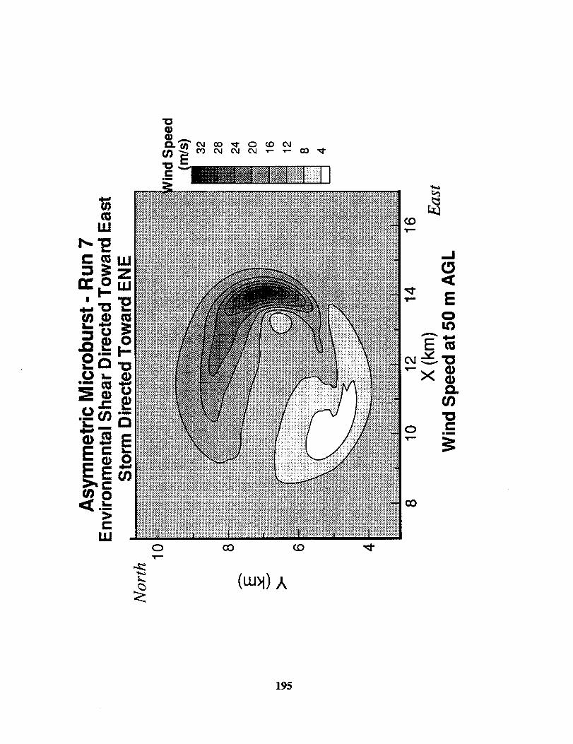
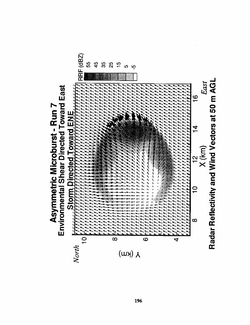
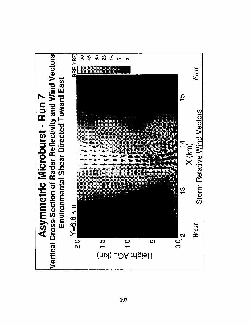
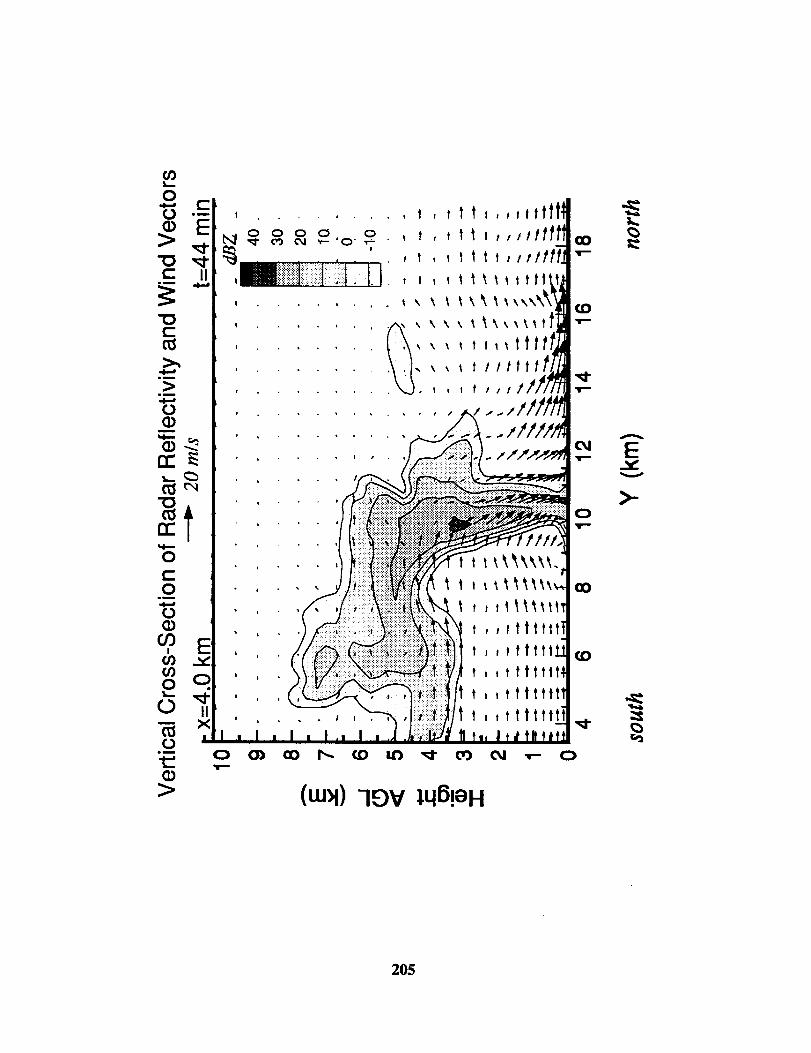
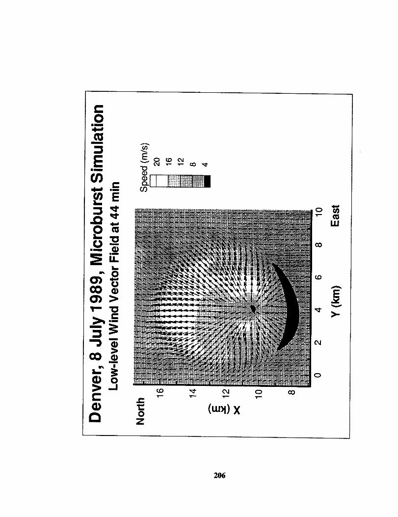
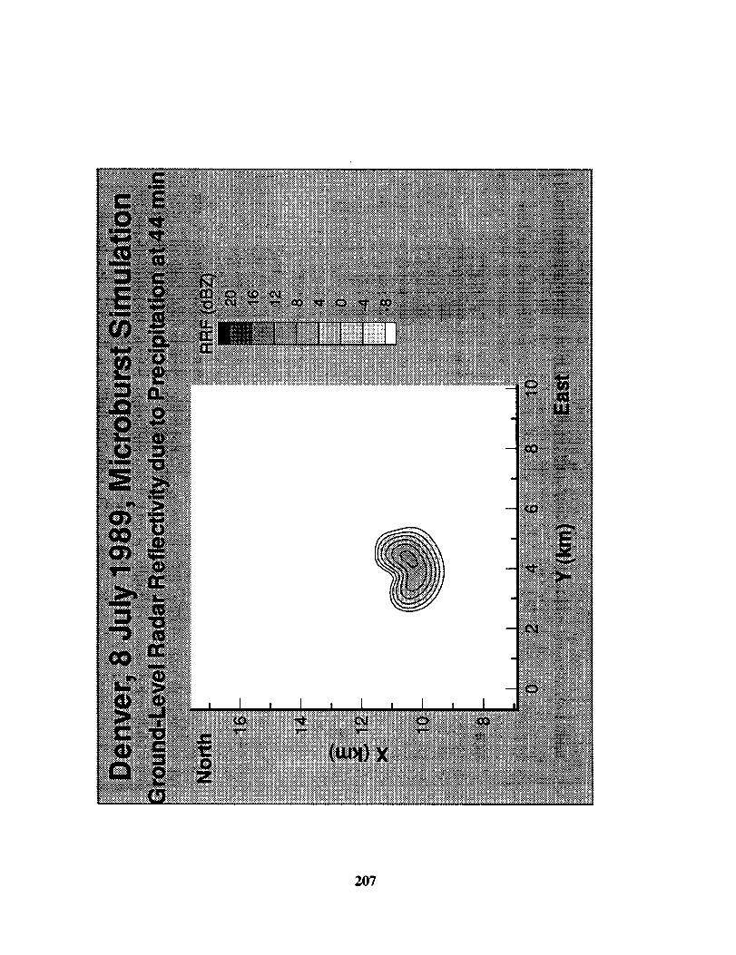
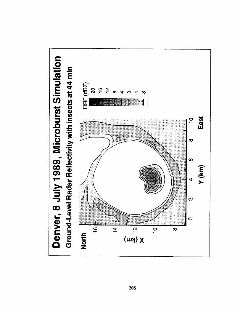
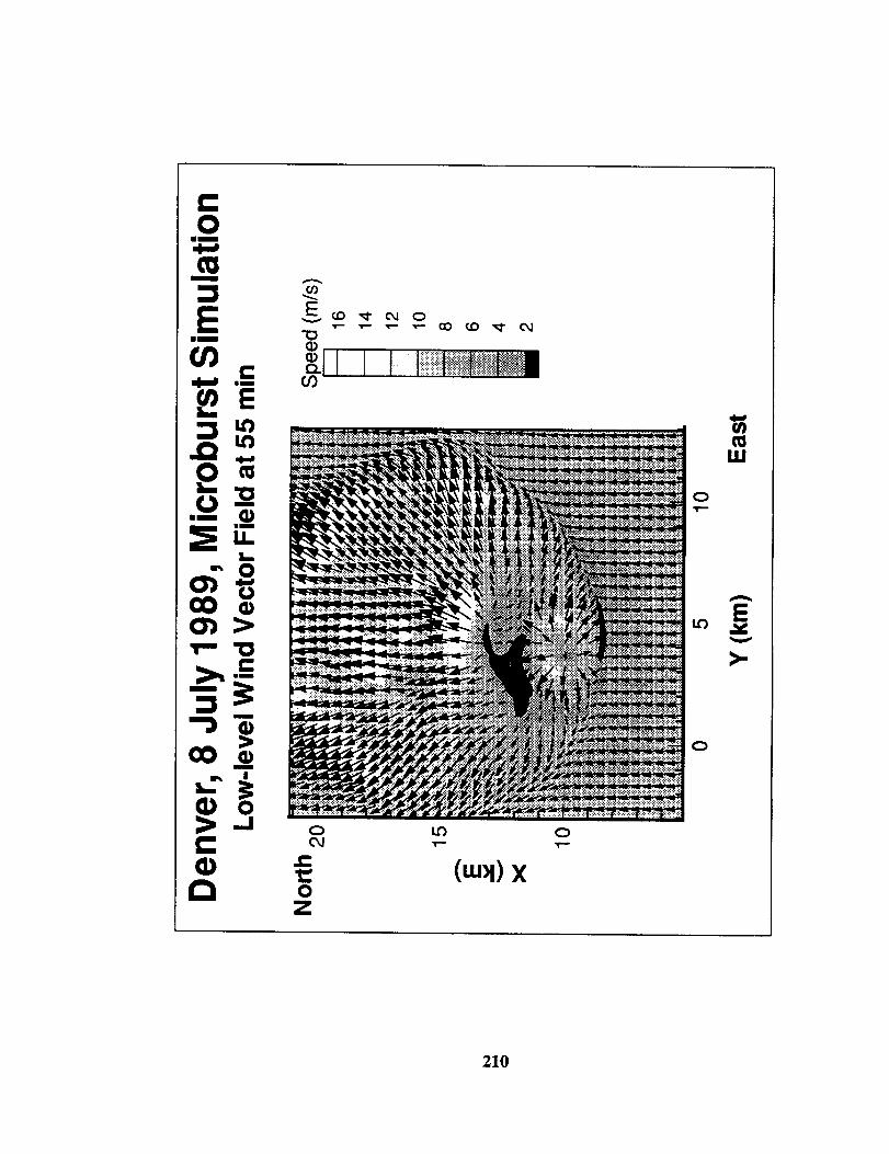
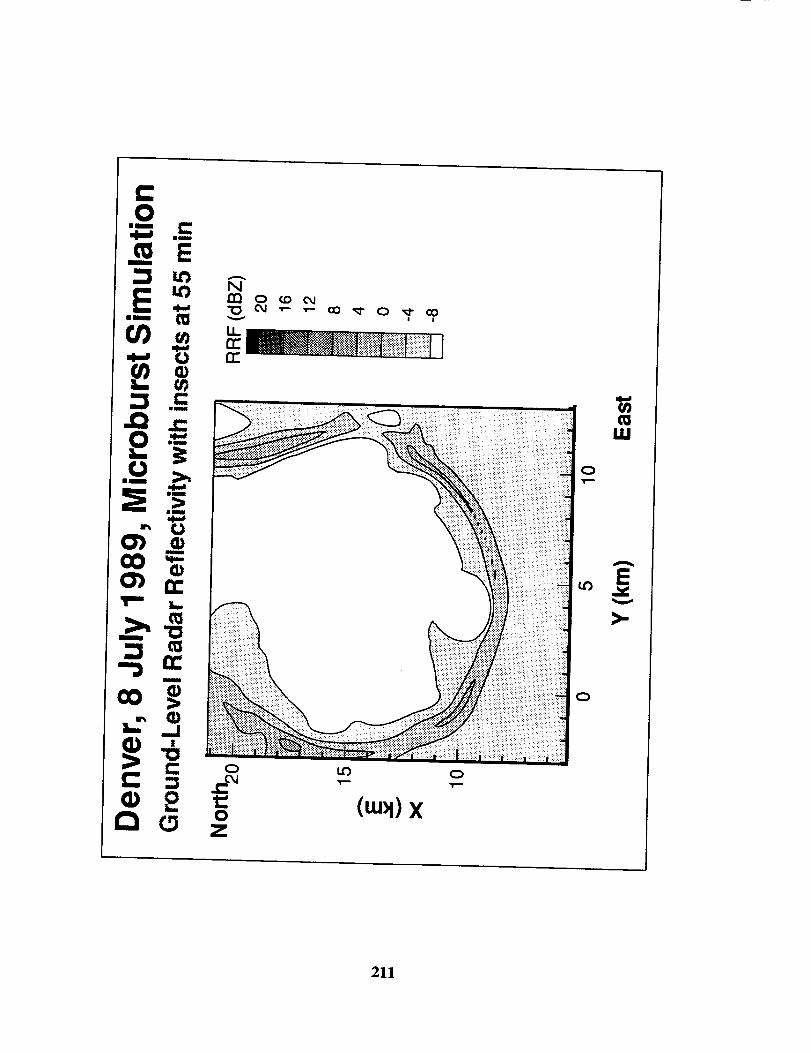
The last series of plots show cross sections from a case with strong ambient shear.

The plots show radar reflectivity and velocity fields from Run 7 at a time near peak

intensity. The ambient shear vector is directed east, although the storm is translating

toward the east-northeast (see table 3). The figures show that the outflow is elongated E-W

along the shear vector. The horizontal cross section of radar reflectivity at low levels

shows a bow-echo shape with maximum radar reflectivity located on the downshear side

of the outflow. The east-west vertical cross section shows a strong vortex circulation on

the downshear side, which is associated with strong surface-level winds. Such a microburst

as in this simulation, may be referred to as what Fujita (1985) calls a "rotor microburst."

185

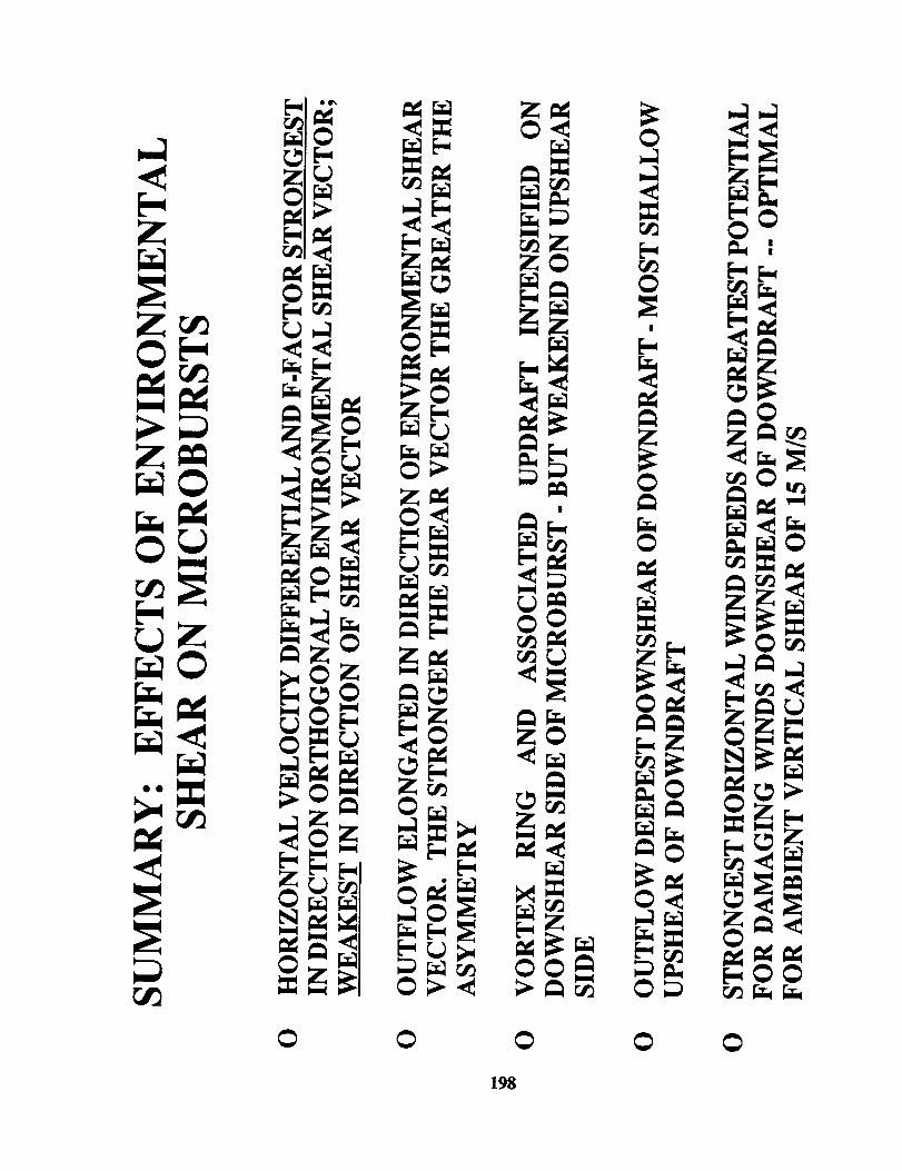
SUMMARY AND DISCUSSION

These results show that microburst asymmetry is influenced by the magnitude of

the low-level ambient vertical shear. The microburst outflow elongates in the direction of

the shear vector (which is not necessarily in the direction of translation), and generates the

greatest hazard (for commercial jet transports) along paths orthogonal to the shear vector.

The model results also show that the asymmetry increases with increasing shear magnitude.

One implication of these results concerns the detection of a microburst by a ground-based

doppler systems. These systems may underestimate the hazard for landing and departing

aircraft that are on trajectories orthogonal to both the sensor beam and shear vector,

especially if the magnitude of the shear is large. Another implication is that microburst are

more likely to be asymmetrical in regions (seasons) where there is climatologically a

significant low-level shear.

The model results also show that rotor microbursts and severe wind damage can be

a product of the microburst interaction with strong ambient wind shear.

186

REFERENCES

Fujita, T. T., 1985: The Downburst, Microburst and Macroburst. University of Chicago

Press, 122 pp.

Proctor, F. H., 1987a: The Terminal Area Simulation System. Volume I: Theoretical

formulation. NASA Contractor Rep. 4046, NASA, Washington, DC, 176 pp.

[Available from NTIS]

Proctor, F. H., 1987b: The Terminal Area Simulation System. Volume II: Verification

Experiments. NASA Contractor Rep. 4047, NASA, Washington, DC, 112 pp.

[Available from NTIS]

Proctor, F. H., 1988: Numerical simulations of an isolated microburst. Part I: Dynamics

and structure. J. Atmos. Sci., 45, 3137-3160.

Proctor, F. H., 1989: Numerical simulations of an isolated microburst. Part H:

Sensitivity experiments. J. Atmos. Sci., _ 2143-2165.

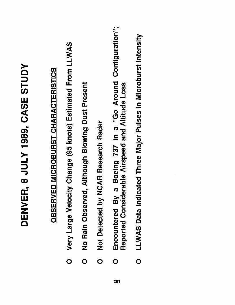
Proctor, F. H., 1993: Case study of a low-reflectivity pulsating microburst: numerical

simulation of the Denver, 8 July 1989, storm. Preprints, 17th Conf. on Severe

Local Storms, St. Louis, Mo., Amer. Meteor. Soc., 677-680.

Proctor, F. H., and R. L. Bowles, 1992: Three-dimensional simulation of the Denver 11

July 1988 microburst-producing storm. Meteorol. and Atmos. Phys., _ 107-124.

Switzer, G. F., F. H. Proctor, D. A. Hinton and J. V. Aanstoos, 1993: Windshear database

for forward-looking systems certification. NASA TM-109012, 133 pp.

Weisman, M. L. and J. B. Klemp, 1982: The dependence of numerically simulated

convective storms on wind shear and buoyancy. Mon. Wea. Rev., 110, 504-520.

Weisman, M. L. and J. B. Klemp, 1984: the structure and classification of numerically

simulated convective storms in directionalIy varying wind shears. Mon. Wea. Rev.,

112, 2479-2498

Weisman, M. L., 1993: The genesis of long-lived bow echoes. J. Atmos. Sci., 50, 645-670.

187

TERMINAL AREA SIMULATION SYSTEM(TASS)

[ALSO KNOWN AS THE NASA WINDSHEAR MODEL]

0 3-D TIME DEPENDENT EQUATIONS FORCOMPRESSIBLE NONHYDROSTATIC FLUIDS

O PROGNOSTIC EQUATIONS FOR 11 VARIABLES0

2.3.

4.

5.6.7.8.9.

10.

3-COMPONENTS OF VELOCITYPRESSUREPOTENTIAL TEMPERATUREWATER VAPOR

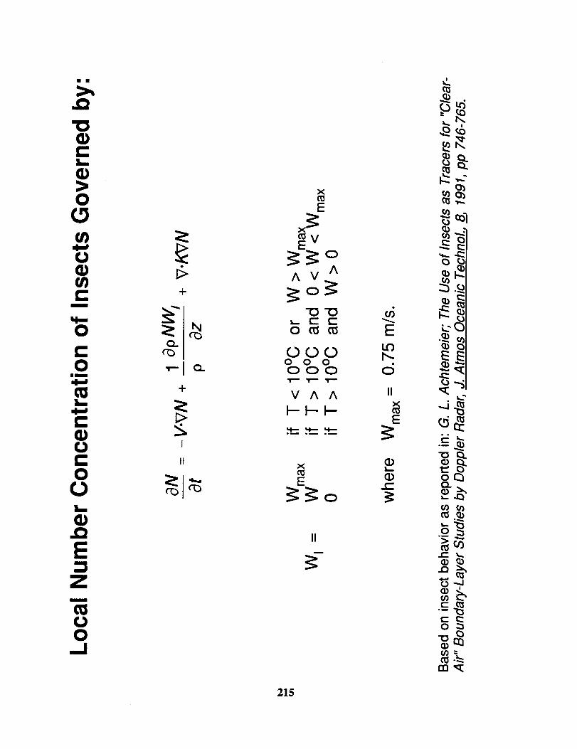
LIQUID CLOUD DROPLETSCLOUD ICE CRYSTALSRAINSNOWHAIL/GRAUPELINSECTS

O 1st-ORDER SUBGRID TURBULENCE CLOSUREWITH RICHARDSON NUMBER DEPENDENCY

O SURFACE FRICTION LAYER BASED ON MONIN-OBUKHOV SIMILARITY THEORY

O Choice At LATERAL BOUNDARIES Between OPEN

BOUNDARY CONDITIONS ALLOWING MINIMALREFLECTION or PERIODIC CONDITIONS

O BULK PARAMETERIZATIONSMICROPHYSICS

OF CLOUD

188

TERMINAL AREA SIMULATION SYSTEM

CAN SIMULATE CONVECTIVE STORMS WITH REASONABLECOMPARISON TO REAL-WORLD EVENTS

O REQUIRES INPUT VERTICAL PROFILE OFTEMPERATURE, HUMIDITY, WIND SPEED ANDDIRECTION, AND ALTITUDE (OR PRESSURE)

O SOUNDING MUST BE REPRESENTATIVE OFSTORM'S ENVIRONMENT

O SOUNDING MAY BE EITHER OBSERVED,FORECASTED (e.g. MASS), OR INTERPOLATED

SIMULATIONS FROM TASS EXTENSIVELY VALIDATEDAGAINST OBSERVED STORMS RANGING FROM

OOOO

SHORT-LIVED WEAK CUMULONIMBUSSEVERE LONG-LASTING SUPERCELL STORMSMICROBURST PRODUCING STORMSHAILSTORMS AND TORNADIC THUNDERSTORMS

189

IX:

I,I,I

_J

t,,)m

I,Ll>

W

,,=,

==

m

:!

it}I-

:Eo

OI--

I.'2 _=I-I-

_,,.0

T" _1"_Z

:bOO o :_z _OO :_nOOe_ ::I: O,,,-. 0. O

,,>,_I

12:

Z:DO

O.OI-I--,,:I:

LIJ

u

n-O

I.I.IIV"O._Im

0

u.

WF-

Z

F-09

0n-O

!--ZILl

Z0Emini

ZILl

!--(/)E

rnoE0

!--!11

190

y

i191

192

i!

I

%b

II

JM

193

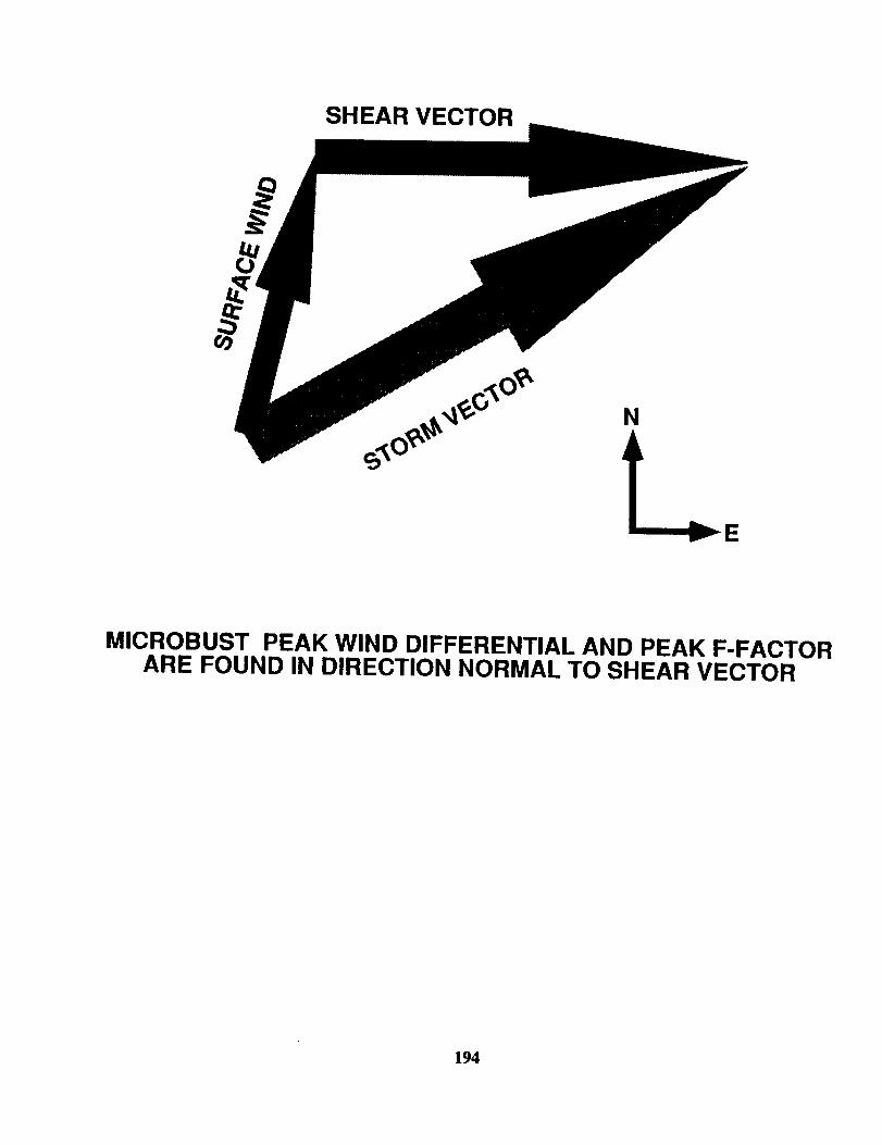
SHEAR VECTOR

N

MICROBUST PEAK WIND DIFFERENTIAL AND PEAK F-FACTORARE FOUND IN DIRECTION NORMAL TO SHEAR VECTOR

194

0

..1

0

Em

"X _

o e,,

195

Nm

LI_

0 CO r.O ._-

0

mi

196

o

CLUiim

2E_

D

t_

mm

A

v

L_

0

0

-0

vX.__

E

197

Z

199

w(

200

Ill

mLI.I 0a

111>

IDm

_1

o?, or- m=30

,_1

1::: a. "a

ill

r,,

CI

o._o

_') 0 o

0 0Z Z

il

Ill

m r_ _"

"_0

r'-(V _j)

O0

e,- _ _j

0 0 0 0 0

201

0II

mI

Im

iii3:

gJ,- F-__ U.

_D

0 Z

t_ -J

°ZI-- LU (/)--i,i • U)on-

.J_U) v

_ oO_ =__DZx __ oO

oo m_=

__ __ oo

>0

__ Z__ _>O_ _ 0=_ _

_=> _0_ __ _0_

_oo _oo _ooo _o_ z

= 0 0 00 0

202

i _

I

I

I

203

$

I _ •

I_ it

I

_. II

• Itl I

IeII

II

204

cO

0

oo

o

(m_l) 19V lqB!aH

1=:V

>..

205

C0

Im

Eim

C

E

U _m

C

C

a

c-

oZ

O4

(uJ_)x

o,,i,=..

co

L/J

00

o4

o

2O6

207

C:0

im C

o 17;"- m

C_

0

208

0Em

m

E

I.O

0 "

U .c_li

E

0

!

--j

CO ",,, 0

I- CO

C_

0 _ _ "-" "-" 0 0 0

U_

(_u_)x

_D

0

209

C0

IIm

t_m

Eiim

in

._o

v- "0

C

v

"0

o

1=0Z

L_

(Ua_l)X

o

I,Ll

o

V

0

210

C0

"--" C

(tml) X

211

C0

BR

2

v-- U.

m

|

0

r.. z

C_

u') U') u')_- O_ C_ v- _-- 0 0 0 v--

" I" |°

0

LI_

0 _ 0

(_) x

0

I.¢) ,_

0

212

213

v"1"-'

0 0 0 0 0 0

214

000

ZI

0

ffl=

215