Embed Size (px)
Citation preview

State estimation of a hexapod robot using a
proprioceptive sensory system
E. Lubbe
21696888
Dissertation submitted in fulfilment of the requirements for the
degree Magister in Computer and Electronic Engineering at the
Potchefstroom Campus of the North-West University
Supervisors: Dr. K.R. Uren
Co-supervisor: Dr. D. Withey
November 2014

i
SUMMARY
The Defence, Peace, Safety and Security (DPSS) competency area within the Council for Scientific and
Industrial Research (CSIR) has identified the need for the development of a robot that can operate in
almost any land-based environment. Legged robots, especially hexapod (six-legged) robots present a
wide variety of advantages that can be utilised in this environment and is identified as a feasible
solution.
The biggest advantage and main reason for the development of legged robots over mobile (wheeled)
robots, is their ability to navigate in uneven, unstructured terrain. However, due to the complicated
control algorithms needed by a legged robot, most literature only focus on navigation in even or
relatively even terrains. This is seen as the main limitation with regards to the development of legged
robot applications. For navigation in unstructured terrain, postural controllers of legged robots need
fast and precise knowledge about the state of the robot they are regulating. The speed and accuracy
of the state estimation of a legged robot is therefore very important.
Even though state estimation for mobile robots has been studied thoroughly, limited research is
available on state estimation with regards to legged robots. Compared to mobile robots, locomotion
of legged robots make use of intermitted ground contacts. Therefore, stability is a main concern when
navigating in unstructured terrain. In order to control the stability of a legged robot, six degrees of
freedom information is needed about the base of the robot platform. This information needs to be
estimated using measurements from the robot’s sensory system.
A sensory system of a robot usually consist of multiple sensory devices on board of the robot.
However, legged robots have limited payload capacities and therefore the amount of sensory devices
on a legged robot platform should be kept to a minimum. Furthermore, exteroceptive sensory devices
commonly used in state estimation, such as a GPS or cameras, are not suitable when navigating in
unstructured and unknown terrain. The control and localisation of a legged robot should therefore
only depend on proprioceptive sensors. The need for the development of a reliable state estimation
framework (that only relies on proprioceptive information) for a low-cost, commonly available
hexapod robot is identified. This will accelerate the process for control algorithm development.
In this study this need is addressed. Common proprioceptive sensors are integrated on a commercial
low-cost hexapod robot to develop the robot platform used in this study. A state estimation
framework for legged robots is used to develop a state estimation methodology for the hexapod
ii
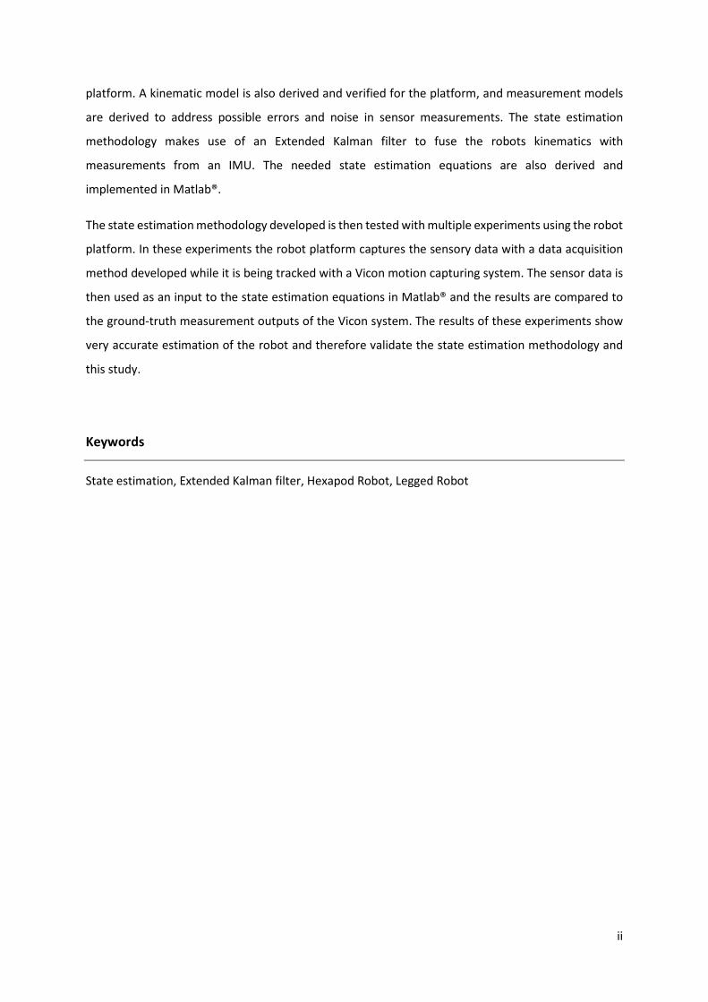
platform. A kinematic model is also derived and verified for the platform, and measurement models
are derived to address possible errors and noise in sensor measurements. The state estimation
methodology makes use of an Extended Kalman filter to fuse the robots kinematics with
measurements from an IMU. The needed state estimation equations are also derived and
implemented in Matlab®.
The state estimation methodology developed is then tested with multiple experiments using the robot
platform. In these experiments the robot platform captures the sensory data with a data acquisition
method developed while it is being tracked with a Vicon motion capturing system. The sensor data is
then used as an input to the state estimation equations in Matlab® and the results are compared to
the ground-truth measurement outputs of the Vicon system. The results of these experiments show
very accurate estimation of the robot and therefore validate the state estimation methodology and
this study.
Keywords
State estimation, Extended Kalman filter, Hexapod Robot, Legged Robot

iii
ACKNOWLEDGEMENTS
Firstly I would like to give all the glory and honour to my Lord Jesus Christ and thank Him for always
giving me strength during this study.
I would like to thank the CSIR for giving me the opportunity to further my studies. I would especially
like to acknowledge the TSO operational group management and my TSO mentor, Stefan Kersop, for
their involvement and contributions towards this study. I would also like to thank the MIAS operational
group for the use of their Vicon system.
I would like extend my sincerest thanks and appreciation to my supervisor at the CSIR Dr. D. Withey,
for sharing with me his vast amount of knowledge and experience in the field of robotics. I truly
appreciate the passionate manner in which he helped and assisted me throughout the duration of my
studies. His guidance and support was essential toward the success of this study. I would like to thank
Dr. K.R. Uren, my university supervisor, from whom I have learned so much about the research
process. His advice always have a way of calming your nerves and helping you to focus on the
important things, not only with regards to the research but also in other aspects of life. I truly
appreciate the effort and time he spend on helping me perfect this dissertation.
I would like to thank my husband Alwyn, for all of his love and support. This dissertation is dedicated
to him. His encouragement and understanding carried me through the tough times. I would also like
to thank my family and especially my parents, Wiaan, Ellie, Elsie and Francois for their support and
understanding.
iv
Table of Contents
SUMMARY ................................................................................................................................................ i
ACKNOWLEDGEMENTS .......................................................................................................................... iii
LIST OF FIGURES ................................................................................................................................... viii
LIST OF TABLES ....................................................................................................................................... xi
LIST OF ABBREVIATIONS AND ACRONYMS ........................................................................................... xii
LIST OF SYMBOLS ................................................................................................................................. xiii
Chapter 1: Introduction .......................................................................................................................... 1
1.1 Background ............................................................................................................................. 1
1.2 Problem statement ................................................................................................................. 2
1.3 Issues to be addressed and methodology .............................................................................. 3
1.4 Contributions made by the study ........................................................................................... 4
1.5 Validation and verification ...................................................................................................... 4
1.6 Overview of dissertation ......................................................................................................... 5
Chapter 2: Literature survey ................................................................................................................... 7
2.1 Introduction ............................................................................................................................ 7
2.2 Background ............................................................................................................................. 7
2.3 Hexapod robots ....................................................................................................................... 8
2.3.1 Background ..................................................................................................................... 8
2.3.2 Important topics surrounding hexapod robots............................................................... 9
2.3.3 Applications ................................................................................................................... 11
2.3.4 Hexapod robot limitations ............................................................................................ 12
2.4 Sensory systems .................................................................................................................... 13
2.4.1 The importance of a sensory system ............................................................................ 13
2.4.2 Sensory system for a hexapod robot ............................................................................ 14
2.4.3 Sensory system development for a hexapod robot ...................................................... 18
2.4.4 Sensory system challenges for a hexapod .................................................................... 19

v
2.5 State estimation of a robot ................................................................................................... 20
2.5.1 Importance of state estimation .................................................................................... 20
2.5.2 Sensory integration and interpretation for state estimation ....................................... 21
2.6 Conclusion ............................................................................................................................. 24
Chapter 3: Literature study ................................................................................................................... 26
3.1 Introduction .......................................................................................................................... 26
3.2 Background ........................................................................................................................... 26
3.3 Hexapod platforms ............................................................................................................... 27
3.3.1 Mechanical characteristics of hexapod robots ............................................................. 27
3.3.2 Commercially available platforms ................................................................................. 29
3.3.3 Platforms considerations .............................................................................................. 32
3.4 State estimation .................................................................................................................... 33
3.4.1 State estimation algorithms .......................................................................................... 34
3.4.2 Proprioceptive state information for a legged robot.................................................... 41
3.4.3 Sensor requirements ..................................................................................................... 41
3.4.4 Sensor considerations for the proprioceptive sensory system .................................... 42
3.5 Conclusion ............................................................................................................................. 46
Chapter 4: Kinematic model ................................................................................................................. 48
4.1 Introduction .......................................................................................................................... 48
4.2 Background ........................................................................................................................... 48
4.2.1 Position ......................................................................................................................... 48
4.2.2 Orientation .................................................................................................................... 50
4.2.3 Frames ........................................................................................................................... 51
4.3 Robotic platform ................................................................................................................... 52
4.4 Kinematic model for a robot leg ........................................................................................... 54
4.5 Kinematic model for hexapod robot ..................................................................................... 61
4.6 Kinematic measurement model ............................................................................................ 64
4.7 Conclusion ............................................................................................................................. 64
vi
Chapter 5: Sensory system.................................................................................................................... 66
5.1 Introduction .......................................................................................................................... 66
5.2 Sensory devices ..................................................................................................................... 66
5.2.1 Joint position Sensors ................................................................................................... 66
5.2.2 MicroStrain 3DM-GX3-25 .............................................................................................. 69
5.2.3 Force Sensors ................................................................................................................ 71
5.3 Sensory system data acquisition ........................................................................................... 72
5.3.1 Data Acquisition Frequency .......................................................................................... 72
5.3.2 Data Acquisition Process ............................................................................................... 73
5.4 Measurement models ........................................................................................................... 75
5.4.1 Joint position measurement model .............................................................................. 76
5.4.2 IMU measurement model ............................................................................................. 77
5.5 Conclusion ............................................................................................................................. 79
Chapter 6: State estimation .................................................................................................................. 81
6.1 Introduction .......................................................................................................................... 81
6.2 Background ........................................................................................................................... 81
6.2.1 The Extended Kalman filter ........................................................................................... 82
6.3 State definition of Extended Kalman filter ........................................................................... 83
6.4 Filter prediction model ......................................................................................................... 86
6.5 Filter measurement model ................................................................................................... 89
6.6 Extended Kalman filter equations ......................................................................................... 90
6.6.1 Filtering convention ...................................................................................................... 90
6.6.2 Prediction step .............................................................................................................. 90
6.6.3 Update step ................................................................................................................. 101
6.7 Conclusion ........................................................................................................................... 104
Chapter 7: Implementation and results .............................................................................................. 106
7.1 Introduction ........................................................................................................................ 106
7.2 Kinematic model and verification ....................................................................................... 106

vii
7.3 State estimation implementation ....................................................................................... 107
7.3.1 Program architecture .................................................................................................. 107
7.3.2 Noise parameters ........................................................................................................ 110
7.3.3 Initialisation ................................................................................................................. 113
7.4 State estimation results ...................................................................................................... 113
7.4.1 Test description ........................................................................................................... 113
7.4.2 Results and discussion ................................................................................................ 116
7.5 Conclusion ........................................................................................................................... 123
Chapter 8: Conclusion and future work .............................................................................................. 125
8.1 Summary of work done ....................................................................................................... 125
8.2 Evaluation of state estimation approach ............................................................................ 126
8.3 Improvements and future work .......................................................................................... 127
8.4 Conclusion ........................................................................................................................... 128
APPENDIX ............................................................................................................................................ 129
Appendix A: Code ............................................................................................................................ 129
Matlab code ................................................................................................................................ 129
Arduino code ............................................................................................................................... 129
Python code ................................................................................................................................ 130
Appendix B: IMU datasheet [74] ..................................................................................................... 136
Appendix C: Force Sensors .............................................................................................................. 138
Data sheet [73] ............................................................................................................................ 138
Circuit .......................................................................................................................................... 139
REFERENCES ........................................................................................................................................ 140

viii
LIST OF FIGURES
Chapter 2
Figure 2. 1: Hexapod configurations: hexagonal (�) and rectangular(�). ............................................ 9
Figure 2. 2: Common hexapedal gait patterns [18], [19]. ..................................................................... 11
Figure 2. 3: Hexapod applications: (�) Messor [20], (�) ATHLETE [21], (�) SILO6 [8], (�) DRL Crawler
[22], (�) RHex [23], () X-RHex [24], [25]. ........................................................................................... 12
Figure 2. 4: Methods for data acquisition [40]. .................................................................................... 23
Figure 2. 5: Taxonomy of data fusion methodologies [42]. .................................................................. 24
Chapter 3
Figure 3. 1: Comparison between an insect (�) and a designed robot leg (�) [47]. ........................... 28
Figure 3. 2: Top view of trunk of the a typical hexapod robot [20] ...................................................... 29
Figure 3. 3: Three segment body design. .............................................................................................. 29
Figure 3. 4: PhantomX Mark II [51] ....................................................................................................... 30
Figure 3. 5: Lynxmotion T-Hex 18DOF hexapod walking robot kit [52]. ............................................... 31
Figure 3. 6: DFRobot hexapod robot kit [53]. ....................................................................................... 31
Figure 3. 7: A general non-linear state space model representation [55]. ........................................... 34
Figure 3. 8: A block diagram of a linear state space model [55]. .......................................................... 35
Figure 3. 9: Kalman filter loop [55]. ...................................................................................................... 36
Chapter 4
Figure 4. 1: Position vector relative to a coordinate frame. ................................................................. 49
Figure 4. 2: Translation of a point. ........................................................................................................ 49
Figure 4. 3: Location and orientation of a point relative to a reference system. ................................. 50
Figure 4. 4: Rotation of a point about the axis by θ degrees . .......................................................... 51
Figure 4. 5: Right-hand rule. ................................................................................................................. 52
Figure 4. 6: Robot prototype with integrated sensors.......................................................................... 53
Figure 4. 7: Location of the IMU on the robot platform. ...................................................................... 54
Figure 4. 8: Top view of robot with servo motor ID's. .......................................................................... 54
Figure 4. 9: Example of a revolute joint. ............................................................................................... 55

ix
Figure 4. 10: The relationship between the sectional view of the robot leg and the links and joint axes.
.............................................................................................................................................................. 55
Figure 4. 11: Example of allocation of the four link parameters. ......................................................... 56
Figure 4. 12: Parameter and link-frame assignment from the robot Leg. ............................................ 58
Figure 4. 13: Location of intermediate frames {J}, {K} and {L}. ............................................................. 59
Figure 4. 14: Relationship between the body coordinate frame and origin of legs. ............................ 62
Chapter 5
Figure 5. 1: Angle feedback of a Dynamixel AX12 servo. ...................................................................... 67
Figure 5. 2: Relationship between the leg structure and link location. ................................................ 68
Figure 5. 3: MicroStrain 3DM-GX3-25 inertial sensor [79]. .................................................................. 70
Figure 5. 4: A201 FlexiForce sensor. ..................................................................................................... 72
Figure 5. 5: Robot Platform Captured by High Speed Camera (left photo = first frame). .................... 73
Figure 5. 6: Data acquisition program architecture. ............................................................................. 74
Figure 5. 7: Density function [81]. ......................................................................................................... 76
Chapter 7
Figure 7. 1: Robot platform assembly model. ..................................................................................... 107
Figure 7. 2: State estimation program architecture diagram. ............................................................ 108
Figure 7. 3: Robot platform with Vicon markers................................................................................. 114
Figure 7. 4: Vicon software environment. .......................................................................................... 115
Figure 7. 5: Comparison of the estimated position and the Vicon position outputs for ripple gait. .. 116
Figure 7. 6: Comparison of the estimated position and the Vicon position outputs for tripod gait. . 117
Figure 7. 7: Comparison between the z position estimation of the ripple and tripod experiment. ... 117
Figure 7. 8: Comparison between the estimated z position and the z position outputs of the Vicon
system. ................................................................................................................................................ 118
Figure 7. 9: Comparison between the estimated Z axis velocity and the numerical z-position derivatives
of the Vicon output. ............................................................................................................................ 118
Figure 7. 10: Comparison between the estimated yaw, pitch and roll angles and the orientation
outputs of the Vicon system. .............................................................................................................. 119
Figure 7. 11: Comparison between the estimated yaw and position and the Vicon system's yaw and
position outputs for small turns by the robot. ................................................................................... 120

x
Figure 7. 12: Comparison between the estimated yaw and position and the Vicon system's yaw and
position outputs for large turns by the robot. .................................................................................... 120
Figure 7. 13: Comparison between the estimated velocity and the Vicon system’s numerical position
derivatives for the robot navigating using ripple gait. ........................................................................ 121
Figure 7. 14: Comparison between the estimated velocity and the Vicon system’s numerical position
derivatives for the robot navigating using tripod gait. ....................................................................... 122
Figure 7. 15: Comparison of the position estimation of the centre of body and feet of leg 1, 4 and 5,
and the Vicon system’s position outputs for the centre of the robot body. ...................................... 123
Appendix B
Figure B. 1: Comparator circuit with force sensors. ........................................................................... 139

xi
LIST OF TABLES
Chapter 2
Table 2. 1: Summary of hexapod application goals and their sensors ................................................. 14
Chapter 3
Table 3. 1: Hexapod platform trade-off study ...................................................................................... 33
Table 3. 2: Sensor requirement analysis ............................................................................................... 42
Chapter 4
Table 4. 1: Link Parameter Values. ........................................................................................................ 57
Table 4. 2: Measurements used to derive the robot kinematic model. ............................................... 63
Chapter 7
Table 7. 1: Final standard deviation values of the noise parameters. ................................................ 112
Table 7. 2: RMS error values for ripple and tripod gait velocities. ..................................................... 121

xii
LIST OF ABBREVIATIONS AND ACRONYMS
3D Three dimensional
Bps Bites per second
CAD Computer-aided design
CSIR Council for Scientific and Industrial Research
DOF Degrees of freedom
DIY Do it yourself
DPSS Defence, Peace, Safety and Security
EKF Extended Kalman filter
GPS Global positioning system
ID Identifier
IDE Integrated development environment
IO In-out
IMU Inertial measurement unit
LiPo Lithium Polymer
OCEKF Observability Constrained Extended Kalman filter
PC Personal computer
PSD Power spectral density
pdf Probability density function
PS2 Play Station 2
RC Remote Control
RMS Root mean square
ROS Robot Operating System
SLAM Simultaneous Localisation and Mapping
TTL Transistor-transistor logic
UKF Unscented Kalman filter
USB Universal Serial Bus
VMCS Vicon Motion Capture System
xiii
LIST OF SYMBOLS
Lower-case symbols Unit Description
� m/s� Absolute acceleration � m Link length � - Bias vector � - Bias parameter
�� m/s� Acceleration bias
�� rad/s Angular rate bias �������� - Initial bias ���_��� - In-run bias
� m Link offset � !(∙) - Quaternion exponential map # - Process dynamics function or prediction model $%& ' IMU output acceleration quantity
m/s� Proper acceleration
( m/s� Measured proper acceleration )(∙) - Density of a variable
* m/s� Gravity vector
' m/s� Physical unit of g-force acceleration
*+ m/s� Local measured gravity vector
'� m/s� Local gravitational acceleration , - Process observation or measurements model ℎ m Altitude above sea level . - General index / s Discrete time step 012 - Kinematic model 2 - Measurement noise vector 2� - Transformed measurement noise quantity

xiv
23 m Discrete kinematic model Gaussian noise 24 rad Discrete joint position Gaussian noise ! - Probability 5 m Robot foot position 6 - Centre of robot body quaternion 67 - Centre of robot body quaternion estimate 8 m Centre of robot body position 9 m Foot contact position vector with respect to : 9; m Measured position vector of foot contact with respect to : < s Continuous time ∆< s Time step (∆< = <?@A + <?) C - Process input vector D rad Euler angle vector E m/s Centre of robot body velocity F - State noise vector
F� m/s�/√Hz Continuous additive acceleration white Gaussian noise
F� rad/s/√Hz Continuous additive angular rate white Gaussian noise
FJ� m/sK/√LM Continuous white Gaussian noise (of acceleration bias)
FJ� rad/s�/√Hz Continuous white Gaussian noise (of angular rate bias) FN m Foot slippage white noise term
O - Measurements vector or measurement residual O7 - Predicted measurement P - State vector P7 - State estimate vector P7@ - Update or a posteriori state vector P7Q - Predict or a priori state vector R - Random variable ∆P - Correction vector
xv
Upper-case symbols Unit Description
S - Process input matrix : - Body coordinate frame T - Rotation matrix U - Expected value V - Process dynamics matrix VW - Continuous linearised error dynamics matrix V? - Discrete linearised error dynamics matrix X(∙) - Distribution a variable Y - Translation vector operator Z(∙) - Gaussian distribution [ - Process observations/measurements matrix $ - Inertial coordinate frame \ - Identity matrix ] - Jacobian ]?�� - Jacobian of the kinematic model ^ - Kalman gain matrix _̂ - General axis rotation parameter `W - Continuous noise Jacobian a ° Latitude c - Origin of a frame d m Position vector e - Covariance matrix e@ - Update or a posteriori covariance matrix eQ - Predict or a priori covariance matrix f(∙) - Quaternion matrix map g - Process noise covariance matrix gW - Continuous process noise covariance matrix g? - Discrete process noise covariance matrix gJ� - Covariance matrix for the noise term F�

xvi
gJ� - Covariance matrix for the noise termF�h g� - Covariance matrix for the noise term F
g� - Covariance matrix for the noise term Fh i - Measurement noise covariance matrix i� - Covariance matrix for the measurement noise quantity 2� i3 - Covariance matrix for the noise term 29 i4 - Covariance matrix for the noise term24 ℝ - Real number R - Resistor variable l - Residual covariance matrix m - Transformation matrix operator V - Voltage variable
o_ - p-axis unit vector
pq - p-axis orientation descriptor
r_ - s-axis unit vector
sq - s-axis orientation descriptor
_ - t-axis unit vector
tu - t-axis orientation descriptor
Greek symbols Unit Description
v rador° Link twist x - Rotation variable y - Auxiliary quantity
z�� m/s� Acceleration bias error vector
z�� rad/s Angular rate bias error vector zP - State error vector z5 m Robot foot position error vector z6 - Centre of robot body quaternion error vector z8 m Centre of robot body position error vector

xvii
zE m/s Centre of robot body velocity error vector z{ rad Centre of robot body rotation error vector | - Mean } rador° General angle variable }3~��� rador° Joint position measured by position sensor }����3���~� rador° Translated joint position � rad Joint angles vector
�� rad Joint position measurement vector � - Standard deviation
�� - Variance { rad Rotation vector h rad/s Angular rate h� rad/s Measured angular rate � - Vector to 4 × 4 matrix map
Additional superscript Description
× Skew-symmetric operator � Matrix or vector translation operator −1 Inverse ^ Estimate + Update or a posteriori state − Predict or a priori state
Additional subscript Description
� Continuous � Discrete � Vicon reference frame

xviii

Chapter 1: Introduction
1
Chapter 1: Introduction
“Growth means change and change involves risk,
stepping from the known to the unknown.”
~ Author Unknown
1.1 Background
The Defence, Peace, Safety and Security (DPSS) competency area within the Council for Scientific and
Industrial Research (CSIR) has identified the need for the development of a robot that can operate in
almost any land-based environment. Legged robots present a wide variety of advantages that can be
utilised in this environment and is identified as a feasible solution. In comparison to other legged
robots, hexapod (six-legged) robots exhibit robustness, even with leg defects. They can maintain static
stability on a minimum of three legs and can support more weight than bipeds (two-legged) and
quadrupeds (four-legged).
The biggest advantage and main reason for the development of legged robots, is their ability to
navigate in uneven, unstructured terrain. However, upon investigation it was found that most
literature only focus on legged robots walking on relatively even terrain. This limitation surfaced due
to the complicated control algorithms needed in order for a legged robot to navigate in unstructured
environments. Such control algorithms need to deal with static and dynamic stability of the robot,
terrain model acquisition, path and adaptive feet trajectory planning as well as energy consumption
minimisation, to name a few. The performance of these control algorithms rely on accurate sensory
data and reliable state estimation.
The research and development of control algorithms for legged robots are constrained by the time
and effort spend on the development of a robot platform with reliable state estimation. This
statement is further validated by [1], where, it is stated that economic and human resources are taken
away from the main focus of a robotic project due to research relying on custom designed hardware.
The need for the development of a reliable state estimation framework for a low-cost, commonly
available hexapod platform is identified. This will accelerate the process for control algorithm
development.
Chapter 1: Introduction
2
Even though state estimation for mobile robots has been researched thoroughly, limited research is
available on state estimation with regards to legged robots. Navigation in unstructured terrain
increases the demands on state estimation for legged robots. Postural controllers of a legged robot
need fast and precise knowledge about the state of the robot they are regulating [2]. In contrast to
mobile robots, six degrees of freedom pose information about the robot base is needed in order to
control a legged robot [3]. This is because locomotion of a legged robot makes use of intermittent
ground contacts, making stability a main concern.
The sensory devices used for state estimation of legged robots is also a topic of concern. Since legged
robots have limited payload capacities, any extra devices on the robot, including sensory devices,
should be kept to a minimum. Furthermore, exteroceptive sensory devices commonly used in state
estimation, such as a GPS or cameras, are not suitable when navigating in unstructured terrain [3].
Not only is the information they provide not accurate enough for stability control of a legged robot,
loss of signal with regards to a GPS, or loss of light with regards to a camera, will induce errors in the
state estimation. The control and localisation of a legged robot should therefore only depend on
proprioceptive (internal) sensors. (Exteroceptive sensors can be used to improve the state estimation
done by proprioceptive sensors, but control and localisation should not rely on exteroceptive
information.)
1.2 Problem statement
The purpose of this study is to develop and implement a state estimation methodology of a hexapod
robot platform using only proprioceptive sensors. Emphasis is placed on the contribution this study
will make towards future projects focussing on control approaches for a hexapod robot platform. The
methodology will be implemented on a low-cost commercially available hexapod robot by using
commonly available proprioceptive sensors.
The study will require the development of a hexapod platform by integrating one commercially
available hexapod robot with a sensory system. The sensory system will consist of a combination of
proprioceptive sensors needed for the state estimation. A method for the sensor data acquisition will
also be derived and implemented. For state estimation, a kinematic model of the robot platform is
essential.
Different state estimation frameworks for legged robots will be studied in order to derive the state
estimation equations needed for the hexapod platform. The state estimation equations should
provide accurate six degrees of freedom information about the robot base to make it usable for

Chapter 1: Introduction
3
stability control. The state estimation equations will be implemented and validated for the developed
robot platform.
1.3 Issues to be addressed and methodology
In this study, the state estimation of a hexapod robot using a proprioceptive sensory system, can be
divided into five main components:
The first component involves the acquisition of a hexapod robot. The design of the robot will directly
influence its capabilities. Through a literature study, knowledge on the mechanical characteristics and
the impact these characteristics have on a robot’s performance will be obtained. Thereafter, different
commercially available hexapod robots will be compared in order to determine the best solution.
Factors like the robot’s size, payload capabilities, quality, cost and available information will need to
be considered. The ease with which the software and hardware of the robot can be modified, will also
be investigated.
The second component involves a study on state estimation. Common state estimation algorithms will
be studied. An in-depth review about different state estimation frameworks for legged robots to be
conducted. From this review, a possible approach for the state estimation of this study will be
identified.
The third component involves the sensory system. A review on hexapod sensory systems will be
conducted in order to identify the common sensory devices needed by hexapod robots. Taking into
consideration the possible state estimation approach, different sensor types needed for the state
estimation will be identified. Sensory specifications will be investigated and sensory devices will be
acquired. The sensory devices will then be integrated onto the commercial robot along with a single
board computer that will handle the sensor data acquisition. A software program for the data
acquisition will be developed.
The fourth component involves the state estimation approach. The state estimation equations will be
derived for the hexapod platform. The equations will be implemented in Matlab®. Using the sensor
data of the robot platform, the state estimation methodology will be evaluated.
The fifth and last component involves the validation of the study. Here, emphasis will be placed on
the verification of the state estimation equations and the validation of the state estimation
methodology. The accuracy of the kinematic model derived will also be verified.

Chapter 1: Introduction
4
1.4 Contributions made by the study
The completion of this study will introduce a number of contributions. The use of an inexpensive
(hobby class) commercially available hexapod platform plays an important role in the value of this
study. This allows anyone to implement the findings in this study and as a result have a platform on
which control algorithms can be developed, implemented and tested. This is also true with respect to
the development of the sensory system where low-cost commercially available sensors will be
implemented.
The state estimation framework presented in, “State estimation for legged robots – Consistent fusion
of leg kinematics and IMU.” by Bloesch et al. [2] will play a major role in this study. Although it is stated
that their Observability Constrained Extended Kalman filter (OCEKF) can be implemented for state
estimation on various kinds off legged robots, simulations and physical tests were only conducted on
a quadruped robot by Bloesch et al. [2]. Recently, a simulation test was also conducted on a humanoid
by Rotella et al. [3]. In this study, this state estimation framework will, to the best of the author’s
knowledge, for the first time be adopted for a hexapod and tested with a physical hexapod robot.
Results in the paper presented by Bloesch et al. [2] indicated a drift in the position estimation due to
inaccurate leg kinematics as well as fault-prone feet contact detection. By integrating force sensors in
the hexapod’s feet, one can eliminate any uncertainties and errors created by faulty feet contact
detection. Furthermore, for the implementation of the state estimation, the full kinematic model for
the chosen hexapod robot (PhantomX) will be mathematically derived. To the best of the author’s
knowledge, this derivation has not been published.
1.5 Validation and verification
In order to verify the derived kinematic model, the robot platform will be modelled as an assembly in
SolidWorks®. For specific joint angle inputs the SolidWorks® model’s foot position results will be
compared to the kinematic model’s results. The results obtained from the SolidWorks® model should
be comparable to those of the kinematic model.
The state estimation of the hexapod robot will be validated with a number of physical experiments
involving the robot platform and a Vicon Motion Capture System (VMCS) [4]. Vicon systems are
commonly used throughout the research community to capture motion due to its extreme accuracy.
The Vicon system that will be used consists of twelve cameras that track rigid bodies in 3D space and
capture the information on a network to be used in a Robot Operating System (ROS).
Chapter 1: Introduction
5
A number of experiments will be conducted using the Vicon system and at the same time recording
the state estimation computed by the filter for the robot. The estimated position, velocity, roll, pitch
and yaw of the centre of the robot’s body will then be evaluated with a comparison to the ground
truth measurements provided by the Vicon system.
1.6 Overview of dissertation
Chapter 2 contains a detailed literature review that provides background with respect to the focus of
this study. Important terminology and concepts that were used throughout this study are introduced
and discussed. From the information provided in Chapter 2, the need for this study is identified and a
detailed problem statement is derived.
Chapter 3 contains a detailed literature study on specific topics that were identified in Chapter 2.
Trade-off studies are conducted to support platform and sensory device decisions that were made in
this study. Common state estimation algorithms are discussed and an in-depth literature study about
state estimation for legged robots is provided. The main state estimation framework implemented in
this study is also identified.
The kinematic model needed for the state estimation of the robot platform is derived in Chapter 4. A
leg kinematic model is firstly derived for the legs of the robot platform. The kinematic model, which
describes the forward kinematics of the robot platform, is then derived by transforming the leg
kinematic model into the body coordinate frame. The kinematic measurement model used to describe
specific noise processes needed by the state estimation, is also derived in Chapter 4.
Chapter 5 discusses the specific sensory devices that are integrated onto the robot platform to
perform the state estimation. The method chosen to acquire the sensor data is also discussed. For
each sensory device the measurement model, describing the noise processes needed for the state
estimation, is also derived.
The derivation of the state estimation approach is discussed in Chapter 6. With the use of the
kinematic model, derived in Chapter 4, and the measurement models, derived in Chapter 4 and 5, the
specific algorithm that is used for the state estimation of the hexapod robot platform is derived. The
algorithm fused the kinematics with the sensory data to produce the full body estimate of the robot.
Chapter 7 discusses implementation and results with respect to this study. Firstly, the kinematic model
derived in Chapter 4 is verified. The implementation of the state estimation algorithm is then

Chapter 1: Introduction
6
discussed. The state estimation approach is also validated with multiple experiments that are
compared to ground truth measurements.
In Chapter 8 the dissertation is concluded with a summary of the study outcomes. Possible
improvements are identified and areas for future work are discussed.

Chapter 2: Literature survey
7
Chapter 2: Literature survey
“In literature and in life we ultimately
pursue, not conclusions, but beginnings.”
~ Sam Tanenhaus
2.1 Introduction
Chapter 2 contains a literature survey of research related to this study. Specific background
information that led to the author’s inspiration to conduct this study as well as vital terminology and
concepts are discussed. The chapter contains background information regarding hexapod robots,
important topics surrounding them, hexapod applications as well as their limitations. Literature
regarding the importance of sensory systems, their application in hexapod robots as well as the
sensory feedback expected for a hexapod robot is also discussed. The chapter concludes by addressing
the importance of state estimation for a robot. Here, sensor integration and interpretation, more
specifically, multiple sensors as an information source and multisensor data fusion, is discussed.
2.2 Background
The field of biomimetic robotics, where biological creatures are used as inspiration for innovative
robot design has been steadily developing throughout the years. The mimicking of biological creatures
in terms of their functionality, movement, operation and intelligence has played a vital role in
developing more advanced robots and using them for advanced applications. This is especially evident
with regards to legged robots.
Research conducted in 1986 identified the need for exploring legged robots based on two motivations
[5]. The first is mobility, based on the need for locomotion in uneven, unstructured terrain. This
includes the idea that the path of the feet or legs of the robot can be decoupled from the path of the
body or trunk, and therefore legged robots can provide a smooth and stable environment for a
payload on a robot. The second motivation is that it will advance and contribute to the better
understanding of biological creature locomotion.

Chapter 2: Literature survey
8
A great number of research and development have been done in the last decade on multi-legged
robots. Some of the more common configurations are humanoids (two-legged), quadrupeds (four-
legged), hexapods (six-legged) and even octopods (8 legged). The increasing level of capabilities that
are being developed with regards to legged robots has boundless potential. As a result of this,
countless fields, even space science [6], have identified it and are developing legged robot projects.
However, there are still a lot of limitations and problems to overcome regarding legged robots that
need to be resolved by applied research. These limitations are identified and discussed throughout
this literature survey and will provide the reader with context with regard to the derivation of the
specific research problem addressed in this study.
2.3 Hexapod robots
This section provides background on hexapod robots. It discusses important topics surrounding them
as well as the current hexapod applications available. The section concludes with a discussion on the
current hexapod limitations which emphasises the need for this study.
2.3.1 Background
A hexapod robot is a multi-legged robot that walks on six legs. This type of robot shows great
advantages, not only over wheeled robots, but also over other legged robots. This is mainly due to the
fact that they can easily maintain static stability on a minimum of three legs, allowing them to have a
large range of possible movements. It also provides them with the ability to operate on as little as
three legs while their remaining limbs can be utilised for other tasks. Hexapod robots are also more
efficient for statically stable walking than other legged robots [7].
The speed of a statically stable legged robot is theoretically dependent on its number of legs. It is
known that statically stable legged robots already move slow, therefore it is seen as a big advantage
that a hexapod will be faster than a quadruped and a humanoid [8]. Hexapod robots further exhibit
robustness, even with leg defects and can support more weight than bipeds and quadrupeds. Their
robustness and abilities make them the better choice for a broader variety of applications in
comparison to other types of legged robots [9]. For these reasons, hexapod robots were chosen over
other legged and wheeled robots for this study.

Chapter 2: Literature survey
9
2.3.2 Important topics surrounding hexapod robots
2.3.2.1 Design
A substantial amount of research focuses on the modelling and design of hexapod robots [10]. Most
of the developments made in the design of the physical body are inspired from insects and animals
[11]–[13]. The design of a hexapod robot has a direct influence on its capabilities. The body shape
influences features like the static stability whereas the leg distribution can influence the size of the
actuator required [8]. For a legged robot, the robot is in a static stable condition if the centre of gravity
is within the tripod (made by the three ground contact points of the feet) of ground contact [14].
Hexapod robots are typically divided into two categories describing their body, (or trunk) shape and
leg distribution. The first is known as hexagonal or circular and have six axisymmetrically dispersed
legs. The second classification has six symmetrically dispensed legs on two sides and is known as
rectangular [7]. Fig. 2.1 shows a two dimensional top view of both these categories.
Figure 2. 1: Hexapod configurations: hexagonal (�) and rectangular(�). Most of the initial research and development done on hexapod robots was based on the rectangular
configuration and were biologically-inspired by research conducted specifically on the cockroach and
stick insect [13]. Although most research and development is still being done on the rectangular
configuration, researchers has also started looking at the hexagonal configuration for the advantages
it has with respect to turning gait [9].
2.3.2.2 Control
In order for any robot to perform a task it has to be controlled by a control system. Whether a robot
is just remotely operated to move in a direction or operating completely autonomously, some kind of

Chapter 2: Literature survey
10
control system needs to be present. A robot control system consists of many sub-control systems that
can be open- or closed-loop. For a control system of a hexapod walking over uneven terrain it is
important that, for example, the legs are controlled with a closed-loop feedback system. Such a
closed-loop feedback system will make use of a sensory system providing measurements from a
number of different sensors as well as reliable real-time estimates of the robot’s state. This will allow
the robot to balance itself and stay stable.
A number of studies on hexapod robots involve the development and testing of control algorithms
that minimise the robot’s energy consumption [15], plan adaptive footholds [16] and stabilise the
robot while walking [10]. These algorithms all make use of the robot’s sensory system to provide them
with the necessary sensory feedback for state estimation. The sensory system is therefore considered
the feedback foundation, and the state estimation, the information foundation for the control of a
robot. The sensory feedback used for control in hexapod applications will be discussed later in this
chapter.
2.3.2.3 Locomotion
Locomotion is one of the most important topics when it comes to robots. Locomotion of a robot
describes the robot’s ability to move. Gait locomotion of multi-legged robots is the sequence of
movement of the legs, thus the sequence of how and when the legs are lifted. Foothold planning for
locomotion is how and where the feet are placed to position the robot as best as possible to achieve
its goal.
Gait or locomotion planning is one of the most studied problems found in multi-legged robots [3, 5].
This is mainly due to the fact that it is not possible for a remote operator to manually define each leg’s
movement while the robot is walking. The operator of the robot can define where the robot should
go or give the robot a specific goal, but the foothold planning and leg trajectories should be done on-
board [17]. Different possible gaits for different situations have been studied by analysing hexapod
locomotion [7].
Some of the most common gait patterns that are implemented to provide hexapod robots with
locomotion are shown in Fig. 2.2. The black bars in Fig. 2.2 indicate the leg swing for the right-sided
legs, R1-R3, and the left-sided legs, L1-L3, over time.

Chapter 2: Literature survey
11
Figure 2. 2: Common hexapedal gait patterns [18], [19].
2.3.3 Applications
Over the last few years a number of different hexapod applications have been developed. These
robots differ in size, design, functionality and complexity. Most of these robots have been developed
for a specific function or to achieve a specific goal. This is in accordance with the research done by
Minati and Zorat [1], where they state that current robotic research mostly rely on custom designed
hardware. It was found that commercially available solutions are either very expensive and lack
flexibility, or amateur-level, lacking sufficient computational capabilities.
Some examples of the latest hexapod applications can be seen in Fig. 2.3. The Messor robot is a
versatile walking robot used for search and rescue missions [20]. The SILO6 robot is used for
humanitarian demining missions [8]. ATHLETE is a hybrid hexapod with wheels as feet and is used as
a cargo and habitat transporter for the moon [21]. The DLR Crawler is an experimental hexapod
platform used to test different control, gait and navigation algorithms on [22]. RHex [23] and X-RHex
[24], [25] are high-mobility six-legged robots that uses only one actuator per leg to navigate over rough
terrain and overcome obstacles such as stairs .

Chapter 2: Literature survey
12
Figure 2. 3: Hexapod applications: (�) Messor [20], (�) ATHLETE [21], (�) SILO6 [8], (�) DRL Crawler [22], (�) RHex [23],
() X-RHex [24], [25].
2.3.4 Hexapod robot limitations
Even though multi-legged robots show great potential when it comes to handling rough terrain, most
literature ignore this advantage and only focus on walking on flat or slightly uneven terrain where
wheeled systems are superior [26]–[28]. This is due to complicated control algorithms that are needed
for a multi-legged robot to navigate itself in uneven terrain. Such control algorithms usually deals with
model acquirement of the terrain, path planning through the terrain, foothold selection and planning
while moving through the terrain, feet and/or leg trajectories as well as static and dynamic stability
[5], [16], [17].
Information needed by such a control algorithm has to be provided by a state estimation of the robot
using a sensory system on or around the robot. A sensory system for a hexapod can consist of multiple
sensors such as force, distance and vision sensors. These sensors and/or their data are usually fused
together in state estimation algorithms to provide the control system with a broad range of
information that can be interpreted. The design of sensory systems for hexapod robots are restricted
by the limited payload, energy and the on-board computing power of the robot, as well as budget
limits provided for projects [16].
In order to really take advantage of what a hexapod robot has to offer, a lot of research and
development needs to be done on control algorithms that will optimise their performance and
efficiency. Research showed that a lot of time has to be spent on developing a robot platform that has
a good sensory system that provides real-time state estimates, before attempting the control of the
system. This is also shown in [1] where it is stated that most robotic research in the industry and the

Chapter 2: Literature survey
13
academia relies on custom designed hardware. This takes economic and human resources away from
the main focus of a project. These constraints are seen as the biggest limitation for hexapod
development and might serve as demotivation to developers focussing on specific problems like
control algorithms.
Considering the background given regarding hexapod research, it is evident that the development of
the control algorithms for a hexapod depends on the mechanical design (kinematics) and the available
sensory and state estimation information. The role and importance of a sensory system on a robot will
now be discussed to substantiate the research problem.
2.4 Sensory systems
A sensory system in a robot is responsible for processing and providing sensory measurements that
can also be used to provide state estimation information. The main goal of a sensory system can
therefore be described as the transformation of the physical world into a representation where the
information can be interpreted and used.
This section discusses the importance of a sensory system in general, investigates sensory systems
and the specific sensors found in hexapod applications, provides two different approaches to the
development of a sensory system for a robot, and discusses the sensory system challenges regarding
hexapod robots.
2.4.1 The importance of a sensory system
In the field of bionics we observe that animals and insects make use of different sensing mechanisms
to sense their physical condition as well as the environment around them. Data from their sensing
mechanisms can describe conditions such as forces generated, positions and movements of limbs,
including the velocity of limb movements and acceleration of limbs [29]. The data collected by their
sensing mechanisms is then used as information that will be utilised in their navigation judgement
[30]. By looking at nature the importance of a sensory system is evident towards developing any form
of intelligence.
Over the last few decades the sensory systems of insects have been studied and are used as inspiration
in a biomimetic, (or bio-inspired) approach to solve engineering problems [29]. For the development
of legged robots, the biomimetic approach has been shown to produce better solutions than the
traditional engineering design methods. However, these solutions are still far from optimised when
compared to the speed and agility of insects walking over uneven terrain. As discussed previously, the

Chapter 2: Literature survey
14
importance of a sensory system is also made obvious when considering its necessity in any closed-
loop robotic control system.
According to Siciliano and Khatib [31], sensing and estimation are crucial aspects in the design of any
robotic system. Sensing and estimation for a robot can be divided into two categories. The first is
proprioception, meaning, retrieving the state of the robot itself. The second is exteroception, meaning,
retrieving the state of the environment or external world around the robot [31]. In order to acquire
proprioception and exteroception, specific sensors and the integration of these sensors are needed.
The specific sensors needed in a sensory system for a hexapod robot will now be investigated, whereas
the integration of those specific sensors will be discussed in the state estimation section of this
chapter.
2.4.2 Sensory system for a hexapod robot
2.4.2.1 Sensory feedback in hexapod applications
Table 2.1 describes the goals of some relevant hexapod applications and provides the different sensors
that are implemented on them to form their sensory system. This table provides a general summary
to create context regarding sensory feedback for specific applications.
Table 2. 1: Summary of hexapod application goals and their sensors
Hexapod Goal Sensors
(Proprioceptive = green text, exteroceptive = black
text)
ANTON [12]
Control development
platform
• 24 Potentiometers installed in each joint.
• 6 three-component force sensors mounted in
each leg’s shank.
• 2-axis gyroscopic sensor located inside the
body.
• 2 mono cameras in the head of the robot.
LAURON IV [13]
Inspection of
environments not
accessible for
humans or wheeled
robots.
• Three camera systems (stereo, omni-
directional and time-of-flight)
• Inertial sensor system
• GPS sensors
• 3D foot force sensors

Chapter 2: Literature survey
15
• Spring force sensors
• Motor current sensors
Golem [1]
A flexible, scalable,
general purpose
development and
experimenting tool
targeted to
academia, industry
and defence
environments.
• 4 sonar sensors
• 39 infrared proximity detectors distributed
over the entire structure.
• Position and pressure feedback on all axes.
• 4 accelerometers.
• A two-axis magnetic compass.
• 3 Hall Effect sensors.
• 3 cameras.
• 2 microphones.
SensoRHex [32]
Dynamic locomotion
at high speed over
rough terrain.
• Gearhead/motor/encoder units.
• Voltage/current/temperature sensors.
• Hall Effect sensor.
• Inertial measurement node.
• Infrared distance measurement node.
Messor robot [20]
Used for Urban
Search and Rescue
missions.
• Inertial measurement unit (3 accelerometers
and 3 gyroscopes)
• Resistive sensor to determine contact force
with ground.
• Current sensor to determine the torque in
each joint.
• Video camera
• Laser Range Finder
• Structural light system (vertical laser stripe
used for stair climbing)
An overview will now be given on the commonly used types of sensors found in legged robotics. Their
implementation, goals, importance and classification will be discussed:
Kinematic Sensors
Kinematic sensors in legged robots are sensors that can detect the position of a leg. Therefore, they
are classified as proprioceptive sensors. Examples of such sensors include inclinometers that measure
Chapter 2: Literature survey
16
the tilt or angle of an axis, motor/gearhead/encoder units that convert the angular position of the
actuators, and other joint position sensors. Information provided by kinematic sensors can contribute
to estimating the pose of a robot and is very important for the control of the robot [2].
Force Sensors
Force sensors in the form of resistive sensors are typically applied to the feet of legged robots. They
are used to measure the force and torque extended on the robot’s leg and to determine contact of
the feet with the environment. The force and torque in different joints of legged robots can also be
determined by current sensors on the actuator motors [20]. Force sensors are classified as
proprioceptive sensors.
The information provided by force sensors can be used to ensure the operating safety of legged
robots. For example, a sudden decrease in force or loss in friction can indicate that a leg is slipping. In
order to ensure the safety of the actuating motors, the robots maximum payload can also be
determined by force information [20], [33]. Force information and feedback is extremely important
for the control of legged robots, especially for navigation in uneven terrain [27]. Kaliyamoorthy and
Quinn [33] states that a force control strategy is more appropriate for legged robots navigating in
unknown terrain, than a position control strategy.
IMU
An inertial measurement unit (IMU) or inertial sensor, classified as a proprioceptive sensor, is a device
that is used in robotic applications to estimate relative position, velocity and acceleration. It usually
consists of three orthogonal accelerometers and three orthogonal gyroscopes. Accelerometers
measure external forces acting on a robot and gyroscopes measure changes in the orientation of a
robot [31], [34]. The information from an IMU can therefore contribute to the estimation of a legged
robot’s body pose [2]. The combination of accelerometers and gyroscopes can be found in almost all
legged robot applications.
GPS
The global positioning system (GPS) is another device that is very commonly found on robots that
produce similar information than the IMU, but is usually classified as an exteroceptive sensor. A GPS
is a satellite navigation system that usually provides location (global position) and time information to
a robot used for its navigation. The information provided by a GPS is commonly fused with information
from inertial measurement systems to improve position, velocity and acceleration estimation [35],
[36].

Chapter 2: Literature survey
17
Cameras
A camera is a device that records visual images and is classified as an exteroceptive sensor. Different
types of cameras are commonly found on legged robots. Integrated onto a robot, these devices are
usually used to provide information about the robots’ surrounding environment. This information can
be used to detect, avoid and even identify obstacles. Simultaneous Localisation and Mapping (SLAM)
is also commonly implemented using cameras as sensors [20].
Distance measuring sensors
These include sensors such as laser range finders and infrared distance measuring and proximity
detector sensors. Operating on the time of flight principle, these sensors send out light pulses and
measure the time it takes for them to return to determine the distance to a structure. These kind of
sensors are classified as exteroceptive sensors and are mainly used for map building and obstacle
analysis [20].
2.4.2.2 Proprioceptive vs. exteroceptive sensors
The importance of the proprioceptive sensors in a legged robot becomes evident when comparing the
relationship found between the amounts of proprioceptive sensors to the amounts of exteroceptive
sensors found in Table 2.1. This is especially evident in the robot examples that are designed for
application purposes as to those designed for research purposes.
For state estimation, it is commonly found that proprioceptive sensors, such as an IMU, are used in
combination with exteroceptive sensors, such as a GPS [37]. However, the process of gathering
information by using exteroceptive sensors can’t be contained within the robot as in the case of
proprioceptive sensors. Using exteroceptive sensors as important information sources to a system can
introduce a lot of limitations. For example, a GPS can lose its signal due to bad weather or if the device
is indoors, and a camera using light from the visual spectrum will not work in the dark. Most
exteroceptive sensors can also be hacked or jammed resulting in untrustworthy information.
Using a proprioceptive sensory system for state estimation of a robot will reduce these limitations.
Rotella et al. [3] states that for legged robots operating in unstructured environments, exteroceptive
sensors are unfit and the task of control and localization should depend on proprioceptive sensors.
However, by using proprioceptive sensors drift in the position estimate is inevitable since absolute
position and heading can’t be sensed directly [2], [37]. The limitations of the different sensors will
need to be taken into consideration when a sensory system is developed.

Chapter 2: Literature survey
18
2.4.3 Sensory system development for a hexapod robot
The development of a sensory system for a hexapod robot can be done by means of two different
approaches, a systems engineering approach or a biomimetic approach. Both these approaches will
now be discussed, focusing on their methods, limitations and advantages.
The approach taken by most researchers and developers towards the development of a sensory
system for a robot can be summarised in the following sentence: The application and goal of a robot
define the amount and types of sensors that are needed for the robot to operate successfully. This
approach can be described as a systems engineering process [31]. This process includes an analysis of
the system requirements, modelling the environment, determining the system behaviour under
different conditions and lastly, selecting the suitable sensors.
After completing this process, the hardware components have to be assembled and the necessary
software modules for the data fusion and interpretation have to be developed. The system is finally
tested and its performance is analysed. Once the sensory system is constructed, the different
components of the system have to be monitored for the purpose of analysis, debugging and testing.
Quantitative measurements are also required in terms of robustness, system efficiency and time and
space complexity.
Although this approach can deliver great results for a robot with a specific goal or function, it might
not allow the extreme flexibility exhibited by animals. If the robot’s control system is changed at a
later stage, the sensory system might not provide the control system with the needed information in
order for the robot to operate successfully [29].
The biomimetic designing approach does not consider a specific final purpose when designing or
developing a project. Instead, it considers biological features. For legged robots, such as hexapods,
they specifically try to mimic the sensory systems of insects. The main idea behind the biomimetic
developing approach of a sensory system is based on the fact that biological sensors evolve through
adaptation of existing functional capabilities and structures. This is explained with the following
example; a legged creature has to be able to stand, walk and run with its legs, therefore its sensory
feedback loops have to aid in all three of these activities [29].
When developing a biomimetic sensory system for a hexapod, two main challenges have to be
addressed; choosing or designing adequate sensors that are appropriate, and the integration and
interpretation of the sensors to ensure that the sensor signals can be used effectively. But this is not
an easy task. Delcomyn [29] states that walking robots may require more redundancy and variation in
their sensor arrays than what might seem necessary at first. In order to handle signals appropriately

Chapter 2: Literature survey
19
and effectively, the signal processing must be flexible. This implies that certain feedback signals for
some specific behaviour can be suppressed or dampened in order to prevent interference from them
when other sensor information is more relevant at the specific time.
Although a biomimetic approach to the development of a sensory system for a hexapod might result
in a more versatile platform solution, the complexity that goes together with this approach should not
be taken lightly. The quest to mimic nature for better results can therefore be seen as a trade-off
between accuracy and simplicity.
By comparing these two approaches one can make the following conclusion: The biomimetic and
systems engineering approaches have to be combined in some sense. To avoid the development of an
unnecessarily complex sensory system, the systems engineering approach to a minimum amount of
sensors needed to be considered. However, some aspects of the biomimetic approach should be
included in the development of a sensory system to insure the system stays flexible and allow future
adjustments.
2.4.4 Sensory system challenges for a hexapod
For multi-legged robots, sensory systems should provide the robot with measurements to create a
perception of the environment it is surrounded by and of the state of the robot. This should provide a
legged robot with the information it will need to make decisions and adapt to its environment.
Research done by Belter et al. [16] and Kalakrishnan et al. [28] describes terrain mapping and foothold
selection as crucial to the successful navigation and stability of a legged robot. Neither one of these
can be accomplished without measurements from multiple-sensors and the fusion of these sensors.
Allowing the fusion of multiple sensors is a challenge in the development of any sensory system. In
fact, it is such a challenging problem that there exists a number of research fields dedicated to it. This
will be addressed in the state estimation section of this chapter. The fusion of multiple-sensors is not
the only challenge when it comes to developing a sensory system for a hexapod.
In order for a hexapod robot to be useful as a developing platform towards end applications, it has to
operate in real-time. This is an increasingly complex problem in sensory system development due to
added features like the use of many different types of sensors [31], [38], [39]. Software engineering
issues that receive more attention due to this problem include real-time issues, reusability, using
commercial off-the-shelf (COTS) components, reliability, embedded testing and sensor selection [31].

Chapter 2: Literature survey
20
Other important factors to take into account when developing a sensory system for a hexapod include,
as mentioned before, the limited payload of a robot, the available energy on the robot, the on-board
computing power and the cost of the sensors [16].
2.5 State estimation of a robot
For a robot system, state estimation is a methodology which provides the best possible approximation
for the robot’s state by processing available information. It enables the estimation of unmeasured
variables or parameters, filters out noise and predicts the system’s future behaviour by combining the
system information (provided by a mathematical model of the system) and on-line measurement
information (provided by sensors).
In this section the importance of state estimation for legged robots is discussed. Due to its imperative
role in state estimation, the integration and interpretation of sensors is also discussed. Here the focus
is on providing background information on sensor fusion, a process where data from different sensors
are fused together to reduce sensor errors and increase available information provided by sensors.
The accuracy of, and information provided by a state estimation approach depends enormously on
the sensor fusion techniques applied in the state estimation algorithm. An in-depth literature study
on state estimation for legged robots is done in Chapter 3.
2.5.1 Importance of state estimation
For robotic systems, state estimation is vital for process monitoring, where important variables, such
as velocity might not be directly measurable with enough accuracy. It is also important for control
where a system model contains errors such as unmeasured disturbances. With this in mind, robotic
systems mostly make use of state estimation for navigation and stability. For wheeled robots, state
estimation algorithms typically fuses wheel odometry with an exteroceptive sensor such as a GPS to
estimate the robot’s absolute position and yaw. This is done in order to correct errors caused by, for
example wheel slippage.
For the control of a legged robot, the state estimation has to provide information on the full six
degrees of freedom pose of the base of the robot [3]. This translates to the pose in a three dimensional
space which is, translation and rotation on three perpendicular axes. Six degrees of freedom pose
estimation is especially important when the legged robot has to operate in rough, unstructured
terrains with no prior knowledge about the environment. In contrast to wheeled robots, that are
expected to stay stable and in contact with the ground at all times, legged robots interact with their

Chapter 2: Literature survey
21
environment through intermittent ground contacts. Therefore, the controllers of the robot need fast
and precise knowledge of the state of the robot in order for the robot to maintain stability[2], [3].
The needed knowledge for stability of a legged robot is supplied by means of state estimation that
utilise a dynamic model of the robot to provide estimates of variables needed for pose calculation. In
order to increase the accuracy of the pose estimation and at the same time eliminate any errors in
sensor readings, multiple-sensors are used as information sources.
2.5.2 Sensory integration and interpretation for state estimation
2.5.2.1 Multiple-sensors as an information source
Over the last few years the applications and functionalities of robotic systems increased greatly. This
inspired a new trend in robotics, namely intelligent robots. According to [30], the foundation of
intelligent robots is sensor technology. This is due to the fact that an intelligent robot makes use of
sensory data to make informed decisions, to react and to interact.
Multiple-sensors are needed in order for a robot to gather all of the required information [30]. With
new and developing sensor technology being light in weight, low in cost and much more efficient, the
use of multiple-sensors has become very common in applications. In order to take full advantage of
the information that sensors provide, the data has to be inferred. Therefore, they should be
interpreted as a sensory system. If the information gathered from the sensors is interpreted
separately, inter relationships are lost. These relationships can provide a control system with much
more useful information.
A combination of sensors can be categorised as either homogeneous or inhomogeneous, according to
the information that they provide. Homogeneous sensors are sensors that acquire the same or a
comparable physical measurement. These sensors are usually used together to improve the accuracy
of a specific measurement. Inhomogeneous sensors capture different characteristics and their
information has to be pre-processed since it isn’t directly inferable [40]. These sensors are usually
used together to provide estimates of measurements that are not directly represented by them
separately. For example, depth information together with colour information can be used for easier
feature extraction or object classification [41]. The process of multisensor data fusion is applied in
state estimation of a robot in order to use sensor data optimally.

Chapter 2: Literature survey
22
2.5.2.2 Multisensor data fusion
The process of fusing data from sensors is a wide ranging subject and throughout literature many
different terminologies have been used interchangeably to describe it. Examples of these different
terminologies include sensor fusion, information fusion, data fusion, multisensory data fusion and
multiple-sensor fusion [42]. Just as the terminologies differ, there are many different definitions for
multisensor data fusion. According to [43], sensor fusion is a method of integrating signals from
multiple sources. A similar definition is given by [42], where it is seen as a technology that enables the
combination of information gathered from several sources to produce a “unified picture”. A review
done by [44] discusses many different data fusion definitions. They conclude by proposing the
following definition for information fusion; “Information fusion is the study of efficient methods for
automatically or semi-automatically transforming information from different sources and different
points in time into a representation that provides effective support for human or automated decision
making.”
The main motivation for multi-sensor data fusion is described by [40] as the improvement in the
usability and quality of the measurement result. This includes advantages such as better resolution,
improved noise suppression, increased robustness and improved accuracy. For the control of a robotic
system, this means more accurate state estimation resulting in better control of the robot. The fusion
of data from multiple-sensors are studied in numerous fields including signal processing, artificial
intelligence, control theory, mathematical statistics, information theory as well as bionics [30], [42].
Multisensor data fusion systems can be classified according to their sensor configuration as
competitive, complementary and cooperative integration [40]. Competitive integration is when each
sensor in a sensor configuration delivers an independent measurement of the same property.
Competitive integration is used to avoid erroneous measurements and to reduce uncertainty in
measurements. Complementary integration is when the sensors in a sensor configuration do not
measure the same quantity. The sensors can be integrated to provide a more complete image of the
phenomenon under observation and therefore is seen as a solution for incompleteness.
Cooperative integration is when inhomogeneous sensors in a sensor configuration are integrated to
obtain information that wouldn’t be available from the sensors individually. Cooperative integration
eliminates ambiguities and provides increased information of object details. All of these methods are
usually included to some extent in state estimation. Fig. 2.4 provides a visual explanation of these
classifications as methods of data acquisition. Here, coordinate-transformation describes the process
where each sensor’s local frame has to be transformed into a common frame so that fusion can occur.

Chapter 2: Literature survey
23
Figure 2. 4: Methods for data acquisition [40].
Multi-sensor data fusion challenges
There are numerous challenges that make data fusion for a sensory system such a complicated task.
Most of these challenges are caused by the specific data that needs to be fused, their imperfections
and the diversity of sensor technology found in the system [42]. According to Khaleghi et al. [42] the
data fusion methodologies can be categorised based on the challenges that they address. Fig. 2.5
shows the main challenges involved with multiple-sensor data fusion.
From Fig. 2.5 it can be seen that there are four main challenging problems involved with the fusion of
multiple-sensors: data imperfections, data correlation, inconsistencies found in data and
disparateness. Data imperfections describe the level of impreciseness and the uncertainties found in
sensor data. Data correlation is found when the same noise (external) influence the sensors being
fused. This may cause over/under confidence in the fusion algorithm. Data inconsistencies are data
that may resemble errors but are actually correct due to inconsistencies present in the environment.
Disparate data describes a system that used a wide variety of different data sources (different sensors)
to build a global view.

Chapter 2: Literature survey
24
Figure 2. 5: Taxonomy of data fusion methodologies [42].
Multisensor Data Fusion Algorithms
Research done by Sasiadek [43] divides the sensor fusion algorithms into three basic categories. The
first is based on least-squares techniques, the second on probabilistic models and the third is known
as intelligent fusion. The least-squares techniques utilise optimisation theory, uncertainty ellipsoids,
regularization and Kalman filtering. The probabilistic model methods are robust statistics, evidence
theory, recursive operators and Bayesian reasoning. The intelligent fusion involves fuzzy logic, genetic
algorithms and neural networks [43].
The review done by Khaleghi et al. [42], explores data fusion algorithms according to a novel taxonomy
that is based on data-related aspects of fusion. Khaleghi et al. [42] specifically look at the data-related
challenges that are solved with algorithms and provides tables that summarise the different
algorithms, methods and solutions and their characteristics. In robotic systems these algorithms are
used in state estimation approaches to estimate certain variables while filtering out errors and noise
in sensors. Some of the most common state estimation algorithms will be discussed in Chapter 3.
2.6 Conclusion
The literature survey conducted provides a thorough background with regard to the focus of this
study. Important terminology and concepts were introduced and discussed. Hexapod robots were
identified as an important research topic due to of their ability to navigate in unstructured
environments and their advantages over wheeled and other legged robots. The complicated control
algorithms needed by a hexapod robot were identified as the main limitation in hexapod research.

Chapter 2: Literature survey
25
However, literature showed that this limitation is further restricted by the time and resources needed
to develop a platform and provide reliable state estimation of the robot. The importance of a sensory
system, specifically a proprioceptive sensory system was identified for state estimation and stability
control of a legged robot.
In order to address these limitations, this study will focus on implementing a state estimation
approach on a commercially available hexapod platform. This will require a literature study on the
mechanical characteristics of hexapod platforms in order to perform an analysis on the commercially
available platforms. Further, the study will require the development of a proprioceptive sensory
system for a specific platform. An in-depth literature study on state estimation for legged robots will
guide the sensory system development. It will also provide information on the different approaches
and algorithms that can be implemented to compute the state estimation for the hexapod platform.
Due to the deep theoretical background needed in order to derive a state estimation algorithm for a
robot and the amount of time needed for the implementation and testing of the state estimation
algorithm, the state estimation of the robot is the main focus of this study. In the following chapter a
commercial hexapod platform will be chosen, specific proprioceptive sensors needed will be selected
and a suitable state estimation approach will be identified.

Chapter 3: Literature study
26
Chapter 3: Literature study
“Part of the inhumanity of the computer is that, once it is
competently programmed and working smoothly, it is completely honest.”
~ Isaac Asimov
3.1 Introduction
Chapter 3 contains a literature study on specific topics identified in the literature survey chapter. From
a literature study on hexapod platforms the best commercially available platform was selected.
Common state estimation algorithms was discussed followed by an in-depth literature study regarding
state estimation for specifically legged robots. A state estimation framework was also identified for
this study. Lastly, the specific proprioceptive information needed by a legged robot was summarised
and used to draw up the sensor requirements for the development of the sensory system.
3.2 Background
From the literature presented in Chapter 2, it was found that the main reason for the development of
walking robots is to take advantage of their ability to navigate over unstructured terrain. But, the task
of developing a legged robot for that purpose has been identified as very complex. Every design
aspect, from the mechanical and electronic hardware up to the software and control system is time
consuming and needs intricate integration.
The need for a hexapod platform with accurate state estimation using a proprioceptive sensory system
was identified. Based on the need for research on hexapod control algorithms, a decision to use
commercially of the shelf products for this study was made. This will equip other researchers with a
fast and reliable solution to a platform on which control algorithms can be tested and implemented.
The following literature study focusses specifically on all the aspects and knowledge that is needed in
order to do the state estimation for a hexapod robot with a proprioceptive sensory system. Literature
is reviewed regarding hexapod platforms, proprioceptive sensory systems and current state of the art
state estimation. This literature serves as the basis for all the design decisions that were made in order
Chapter 3: Literature study
27
to complete this study. The mechanical platform, the specific sensors and the state estimation
processes will play a vital role in this study.
3.3 Hexapod platforms
In chapter 2 it was identified that the mechanical design of a hexapod robot directly influences some
features of the robot. This will in turn influence the electronic design and thus the sensory system
development. The hexapod platform’s kinematics will also influence the state estimation and the
control of the robot. It is therefore important to look at specific properties in the mechanical design
of hexapods in order to make an informed decision when acquiring a platform for this study.
3.3.1 Mechanical characteristics of hexapod robots
A hexapod robot’s mechanical design mainly consists of two major components namely: the legs and
the body or trunk. Observations from literature that will influence this study are now discussed for
both of these components.
3.3.1.1 Leg design
For legged robots there are two biologically inspired leg configurations. The first resembles those of
animals (leg swing around a horizontal axis) whereas the second resembles those of insects (leg swing
around a vertical axis). For hexapod robots it is found that the insect leg configuration is used more
commonly. This is mainly due to the fact that the insect leg configuration provides better static and
dynamic stability compared to the animal leg configuration [45].
The leg of the stick insect consists of four segments namely: coxa, femur, tibia and the foot (or tarsus).
This results in each leg having four degrees of freedom (DOF). It is found that throughout literature
the foot segment of the leg is neglected in robot design [10], [20], [46]. The main reason for this is
simplification. By eliminating the feet, the number of joints in a hexapod robot reduces from 24 to 18.
This not only decreases the robot’s cost and weight but also simplifies the control and saves energy.
A comparison between an insect leg (with a foot) and a robot designed leg (without a segment
representing the foot) can be seen in Fig. 3.1.
Manoiu-Olaru et al. [45] states that for a legged robot, a successful design mostly depends on the
design of the legs. This is motivated by considering that all aspects of walking by a legged robot are
eventually governed by the limitations of the leg. When evaluating possible hexapod platforms, it is
therefore important to look at leg designs that will impose the least constrains on the walking and

Chapter 3: Literature study
28
allow a maximum range of motion. The legs should further be as light as possible to provide a high
payload/weight ratio [8].
Figure 3. 1: Comparison between an insect (�) and a designed robot leg (�) [47].
3.3.1.2 Body design
As discussed in Chapter 2, a hexapods’ body design is typically either based on a rectangular
architecture or a hexagonal architecture. Although there are several studies that are based on the
hexagonal architecture [9], [10], [21], the rectangular design is more common [8], [13], [15], [20], [48].
Preumont et al. [49] stated that while the hexagonal design, in contrary to the rectangular design, do
not require a special gait in order to change walking direction, its control is more difficult. This is due
to the legs that have different trajectories with respect to the body. Thus, the rectangular architecture
has advantages regarding straight forward gait whereas the hexagonal architecture has advantages in
turning gait [49], [50].
Research done by de Santos et al [8], [15] showed that the rectangular configuration can be optimised
by broadening the section of the trunk where the middle legs are mounted. Last mentioned can result
in a reduction in the energy consumed by the robot and contributes to the robot’s stability. The
influence of this research is made visible when looking at the trunk design of the Messor robot [20]. A
trunk design similar to the trunk of Messor can be seen in Fig. 3.2.

Chapter 3: Literature study
29
Figure 3. 2: Top view of trunk of the a typical hexapod robot [20]
A bio-inspired design where the body consists of three segments resembling insects such as the ant,
has also been studied [12], [47]. This type of design has increased mobility as the body movement can
contribute to stability control of the robot and the overcoming of obstacles. However, the extra weight
is a disadvantage and the extra segments result in more complicated control algorithms. An example
of such a design is shown in Fig. 3.3.
Figure 3. 3: Three segment body design.
3.3.2 Commercially available platforms
In this study the state estimation will be performed on a commercially available platform. The next
section discusses the different low-cost (hobby classified) commercially available platforms from
which one will be chosen for this study.
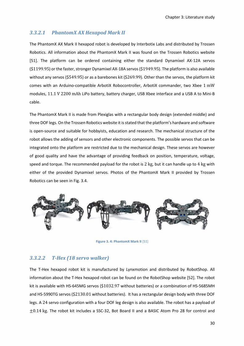
Chapter 3: Literature study
30
3.3.2.1 PhantomX AX Hexapod Mark II
The PhantomX AX Mark II hexapod robot is developed by Interbotix Labs and distributed by Trossen
Robotics. All information about the PhantomX Mark II was found on the Trossen Robotics website
[51]. The platform can be ordered containing either the standard Dynamixel AX-12A servos
($1199.95) or the faster, stronger Dynamixel AX-18A servos ($1949.95). The platform is also available
without any servos ($549.95) or as a barebones kit ($269.99). Other than the servos, the platform kit
comes with an Arduino-compatible ArbotiX Robocontroller, ArbotiX commander, two Xbee 1mW
modules, 11.1V2200mAh LiPo battery, battery charger, USB Xbee interface and a USB A to Mini-B
cable.
The PhantomX Mark II is made from Plexiglas with a rectangular body design (extended middle) and
three DOF legs. On the Trossen Robotics website it is stated that the platform’s hardware and software
is open-source and suitable for hobbyists, education and research. The mechanical structure of the
robot allows the adding of sensors and other electronic components. The possible servos that can be
integrated onto the platform are restricted due to the mechanical design. These servos are however
of good quality and have the advantage of providing feedback on position, temperature, voltage,
speed and torque. The recommended payload for the robot is 2kg, but it can handle up to 4kg with
either of the provided Dynamixel servos. Photos of the PhantomX Mark II provided by Trossen
Robotics can be seen in Fig. 3.4.
Figure 3. 4: PhantomX Mark II [51]
3.3.2.2 T-Hex (18 servo walker)
The T-Hex hexapod robot kit is manufactured by Lynxmotion and distributed by RobotShop. All
information about the T-Hex hexapod robot can be found on the RobotShop website [52]. The robot
kit is available with HS-645MG servos ($1032.97 without batteries) or a combination of HS-5685MH
and HS-5990TG servos ($2130.01 without batteries). It has a rectangular design body with three DOF
legs. A 24 servo configuration with a four DOF leg design is also available. The robot has a payload of ±0.14kg. The robot kit includes a SSC-32, Bot Board II and a BASIC Atom Pro 28 for control and
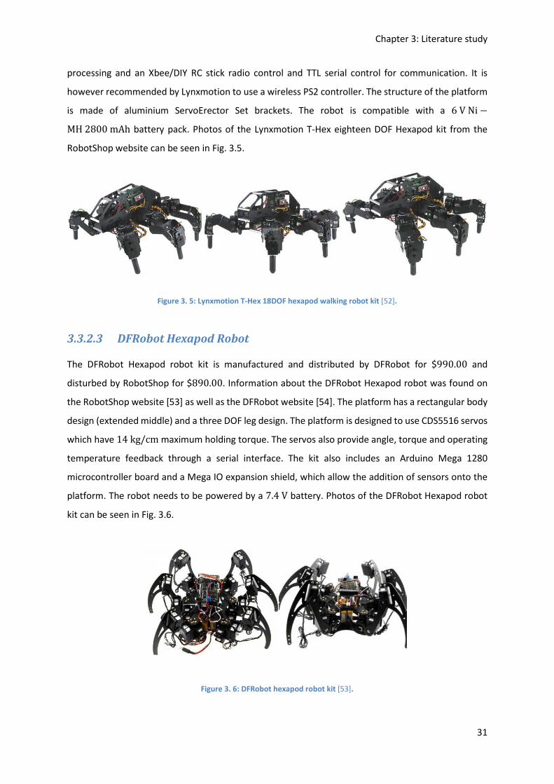
Chapter 3: Literature study
31
processing and an Xbee/DIY RC stick radio control and TTL serial control for communication. It is
however recommended by Lynxmotion to use a wireless PS2 controller. The structure of the platform
is made of aluminium ServoErector Set brackets. The robot is compatible with a 6VNi −MH2800mAh battery pack. Photos of the Lynxmotion T-Hex eighteen DOF Hexapod kit from the
RobotShop website can be seen in Fig. 3.5.
Figure 3. 5: Lynxmotion T-Hex 18DOF hexapod walking robot kit [52].
3.3.2.3 DFRobot Hexapod Robot
The DFRobot Hexapod robot kit is manufactured and distributed by DFRobot for $990.00 and
disturbed by RobotShop for $890.00. Information about the DFRobot Hexapod robot was found on
the RobotShop website [53] as well as the DFRobot website [54]. The platform has a rectangular body
design (extended middle) and a three DOF leg design. The platform is designed to use CDS5516 servos
which have 14kg/cm maximum holding torque. The servos also provide angle, torque and operating
temperature feedback through a serial interface. The kit also includes an Arduino Mega 1280
microcontroller board and a Mega IO expansion shield, which allow the addition of sensors onto the
platform. The robot needs to be powered by a 7.4V battery. Photos of the DFRobot Hexapod robot
kit can be seen in Fig. 3.6.
Figure 3. 6: DFRobot hexapod robot kit [53].

Chapter 3: Literature study
32
3.3.3 Platforms considerations
In order to compare commercial hexapod platforms the following topics have to be considered:
Open-source hardware and software: The ease in which the platform can be modified will have a big
influence on this study. This will allow for more freedom in the sensory system design and
development. It is also seen as an advantage in the sense that the platform can be used for further
research and future work.
Payload: The payload of the robot refers to the amount of weight that can be added onto the platform
without constraining its operational capabilities. It is mainly determined by the mechanical design and
actuator strength. The payload capabilities of the platform will influence the electronic design of the
sensory system as well as the stability margin of the robot. For this reason a higher payload capability
is preferred as opposed to a lower payload capability.
Size: A small sized robot platform (±3kg, fit in a ±0.027mK box) will be used for this study. This is
determined by the size availability of commercial available platforms. A smaller sized platform is also
more cost effective and practical for a research project.
Cost vs. quality: There exist a trade-off between the cost and the quality of a hexapod platform. The
cost of the platform should not have an excessive influence on the platform choice. This will allow the
development of a high quality, robust prototype.
Information: Available information such as the platforms’ kinematics, detailed drawings or a model of
the platform will contribute to the study by minimizing time and effort spent on unimportant tasks
with regards to this study. Detailed drawings will also reduce measurement errors with regards to the
development of the kinematic model for the robot.
Restrictions: Although most commercial hexapod platforms can be ordered without any electronic
hardware, they are still designed to fit specific electronic components. This can influence the robot’s
capabilities by placing limitations on the electronic design. An example of such a limitation is when
the space provided for an actuator in a leg reduces the possibilities in choice of servo motors that can
be integrated onto the platform.
3.3.3.1 Hexapod platform trade-off study
Table 3.1 presents the trade-off study done between the commercially available hexapod platforms.
A score out of ten is given for each platform consideration with regards to each of the platform
options. The weight of each platform consideration was assigned using the information presented in
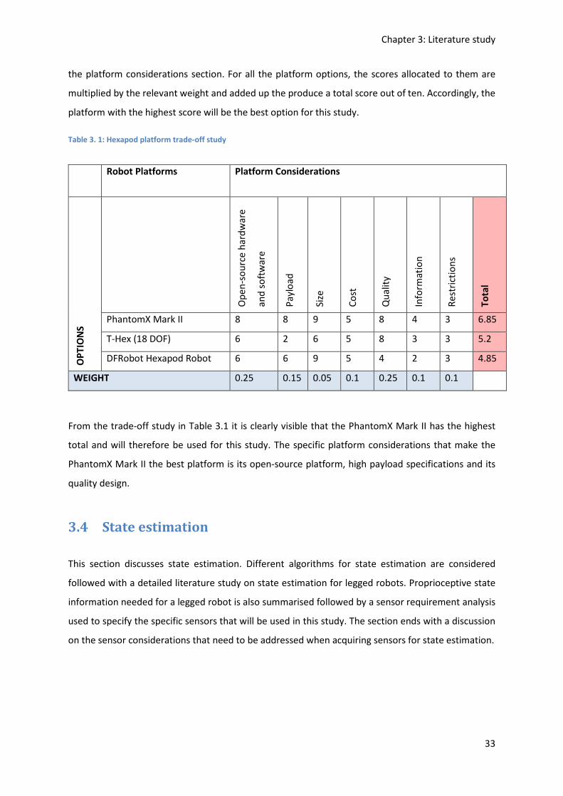
Chapter 3: Literature study
33
the platform considerations section. For all the platform options, the scores allocated to them are
multiplied by the relevant weight and added up the produce a total score out of ten. Accordingly, the
platform with the highest score will be the best option for this study.
Table 3. 1: Hexapod platform trade-off study
Robot Platforms Platform Considerations
OP
TIO
NS
Op
en
-so
urc
e h
ard
wa
re
an
d s
oft
wa
re
Pa
ylo
ad
Size
Co
st
Qu
alit
y
Info
rma
tio
n
Re
stri
ctio
ns
To
tal
PhantomX Mark II 8 8 9 5 8 4 3 6.85
T-Hex (18 DOF) 6 2 6 5 8 3 3 5.2
DFRobot Hexapod Robot 6 6 9 5 4 2 3 4.85
WEIGHT 0.25 0.15 0.05 0.1 0.25 0.1 0.1
From the trade-off study in Table 3.1 it is clearly visible that the PhantomX Mark II has the highest
total and will therefore be used for this study. The specific platform considerations that make the
PhantomX Mark II the best platform is its open-source platform, high payload specifications and its
quality design.
3.4 State estimation
This section discusses state estimation. Different algorithms for state estimation are considered
followed with a detailed literature study on state estimation for legged robots. Proprioceptive state
information needed for a legged robot is also summarised followed by a sensor requirement analysis
used to specify the specific sensors that will be used in this study. The section ends with a discussion
on the sensor considerations that need to be addressed when acquiring sensors for state estimation.

Chapter 3: Literature study
34
3.4.1 State estimation algorithms
3.4.1.1 Background
The processes of a robotic system can mathematically be modelled as state space models [55]. A state
space model consists of a process or prediction model and a measurement model. The prediction
model describes how the state of the process, P, propagates in time based on external influences
(inputs or noises). The measurement model describes how measurements, O, are taken from the
process. For the discrete time step /, a non-linear state space model usually consists of two non-linear
functions, # and ,, such that
P?@A = #(P? , C? , F?), (3. 1)
O? = ,(P? , 2?). (3. 2)
In (3.1), C, represents the process input vector, and F, the state noise vector. In (3.2), 2, represents
the measurement noise vector. The functions, # and ,, usually manage the dynamics of the process
and the observations from the process, and are constructed from a set of discretized differential
equations. Fig. 3.7 represents this general non-linear state space model.
Figure 3. 7: A general non-linear state space model representation [55].
For the functions, # and ,, that are linear in state as well as input, a linear state-space model can be
defined. Therefore, a linear state-space model is based on a linear process. The process can either be
inherently linear or a non-linear process that has been linearised by means of a first-order Taylor
approximation [55]. For a linear state-space model, the state propagation calculations are reduced to
linear algebra by expressing the functions, # and ,, using matrices V, S and [, such that
P?@A = V?P? +S?C? +F? , (3. 3)

Chapter 3: Literature study
35
O? = [?P? + 2? , (3. 4)
where, V, is the process dynamics matrix, S, is the process input matrix, and [, is the process
observations or measurements matrix.
Fig. 3.8 represent a linear state-space model.
Figure 3. 8: A block diagram of a linear state space model [55].
With state estimation the state of a process that isn’t directly observable can be estimated by using
the current state to predict the next, and correcting the prediction by updating it with the noisy
measurement data. This is done by estimating the probability density function (pdf) of the state of the
process. Many different state estimation algorithms exist. Some of the most common algorithms will
now be discussed.
3.4.1.2 Common state estimation algorithms
Recursive Bayesian estimation
Recursive Bayesian estimation is known as the most general form for state estimation and the optimal
way of predicting the state pdf for any process [55], [56]. The recursive Bayesian estimator uses the
estimate of the previous time step, / − 1, together with new measurements to calculate the new
estimate. This is done recursively for each time step in two steps, the prediction step, and the update
step. By using the state propagation belief, !(P?|P?QA), computed from#, the prediction step
extrapolate the current state onto the next time step to predict the next state. The a priori pdf for the
state,P?, at time step /, based on the measurements up to time step/ − 1, is calculated with the
Chapman-Kolmogorov equation, such that [55]

Chapter 3: Literature study
36
!(P?|OA:?QA) = ¥!(P?|P?QA)!(P?QA|OA:?QA)�P?QA. (3. 5)
The update step uses the measurement probability,!(O?|P?), computed from,, to correct the
prediction by taking the new measurements into account [55]. This is done by using Bayes rule,
!(P?|OA:?) = !(O?|P?)!(P?|OA:?QA)¦ !(O?|P?)!(P?|OA:?QA)�P? . (3. 6)
Recursive Bayesian estimation does however not scale well for practical applications and is generally
only considered as a theoretical foundation for state estimation.
Kalman filter
The Kalman filter is the most commonly used approach for state estimation. The Kalman filter reduces
the well-known Bayesian estimation technique by introducing certain constraints on the process
model. Only the mean and covariance of the probability distribution function of the state are
calculated in an optimal way by minimizing the mean square error [57]. The Kalman filter requires the
functions in the state model to be linear, with the noise terms uncorrelated, Gaussian and white with
zero mean. By implementing these constraints, the state model can now be formulated as
P?@A = V?P? +S?C? +F? , (3. 7)
O? = [?P? + 2? , (3. 8)
with V,S and [ matrices that replace # and ,.
The state estimation is then calculated in a two-step process: the prediction step and the update step.
Fig. 3.9 demonstrates the Kalman filter loop where, for time step /, P7?Q represents the a priori state
estimate with covariance matrix, e?Q, and P7?@, represents the a posteriori state estimate with
covariance matrix, e?@.
Figure 3. 9: Kalman filter loop [55].

Chapter 3: Literature study
37
While the Kalman filter is very easy to compute, it is only applicable to linear systems [58]. For non-
linear systems the Extended Kalman filter, the Unscented Kalman filter and the Particle filter are the
most commonly implemented state estimation approaches. Each of these approaches will now be
discussed.
Extended Kalman filter
The need to apply the Kalman filter on non-linear systems, produced what is known as the Extended
Kalman filter (EKF). The EKF linearise the system by calculating the Jacobian of # and , around the
estimated state at each time step [3], [55]. This linearisation method makes use of the first-order
Taylor expansions of the non-linear functions [3], [57]. Thereafter, the estimation is done by applying
the normal Kalman filter equations.
If the consecutive linearisation do not represent a good approximation of the non-linear model, the
algorithm diverges. Therefore, the linear approximation needed for the EKF can introduce errors in
the estimated states and might not be appropriate for some systems [57]. This approach is however
easy to implement and has low computational costs [3], making it one of the most common state
estimators for non-linear systems.
Unscented Kalman filter
Another version of the Kalman filter that can be applied to non-linear systems is the Unscented Kalman
filter (UKF). This approach propagates a set of points, called sigma points, through the non-linear
functions. Where, the points are chosen in such a manner that their mean, covariance and higher
order moments, represent the Gaussian random variable [55].
Since the UKF does not require derivatives, it resolves the limitations brought on by possible errors
introduced in the EKF and is simple and easy to implement [57]. Another advantage observed by
Orderud [55] is that non-Gaussian or non-additive noises can be accounted for since noise can be
handled in a non-linear fashion. György et al. [57] state that the most computational intensive
operation regarding the UKF approach is the calculation of the set of sigma points at each time step.
Particle filters
One of the limitations of the Kalman filters is the fact that they are constrained to model Gaussian
probabilities. Orderud [55] state that they are therefore not capable of handling multimodal or skewed
distributions. In order to estimate non-Gaussian distributions, one of the most common approaches
is Particle filters.

Chapter 3: Literature study
38
The Particle filter approach can best be described as a recursive implementation of the Monte Carlo
based statistical signal processing [57]. By using a set of randomly chosen weighted samples, the
Particle filter approximates the Bayesian posterior probability density function. Here, each sample of
the state is called a particle. Where, a large enough number of particles almost insures convergence
of the true probability distribution function.
Although this approach addresses some of the limitations of Kalman filters, it is more computationally
challenging. Since Particle filters are very computationally intensive, they are often intractable with
regard to usage in real-time settings [55].
3.4.1.3 State estimation for a legged robot
Although state estimation is a broad research field with regards to wheeled robots, only a number of
papers addresses it for legged robots. Also, in most of the research the walking of the legged robot is
limited to structured and well-defined environments. Up to date, research presented for estimating
the pose of a legged robot usually addresses the problem by using information from the environment
outside and the robot itself. This information is provided by specific sensors and the fusion of those
sensors.
However, as stated in Chapter 2, the robust state estimation for a legged robot should not rely on
exteroceptive information and produce a full body pose estimation (6 DOF). With regard to legged
robots, ultimately the robot needs to be fully autonomous and operate without having any knowledge
of the terrain. This is especially evident with regard to small legged robots that can’t carry heavy
distance lasers to map the environment such as Ambler [59] and Dante II [60]. Also, the robot, and
therefore the state estimation and control, should not be restricted to a specific gait pattern. The
following literature was found regarding the state estimation of legged robots.
Gassmann et al. [61] stated that for unstructured terrain, legged robots need knowledge of their
spatial position and their orientation. They based this statement on the observation that there is no
complete a priori knowledge of the robot’s operating environment conditions. They introduced a
method that uses a Kalman filter to estimate absolute position and orientation information for a
hexapod robot by using odometry calculations together with an IMU and a GPS. The odometry
calculations were used to provide permanent basic relative measurements. The IMU was used to
obtain information on the absolute spatial orientation. Although the method presented by Gassmann
et al. [61] is able to provide the robot’s global position, it makes use of a GPS (exteroceptive sensor)
and is not able to handle non-statically stable gaits.
Chapter 3: Literature study
39
The pose estimation approach taken by Lin et al. [23] can handle non-statically stable gaits by fusing
data from a IMU with a leg-strain-based model. The leg-strain-based model provides reliable position
information while the robot has ground contact and isn’t slipping, and the IMU provides continuous
velocity information. Their approach accurately estimate body position and orientation for a hexapod
robot but only when the robot has tripod ground support.
Chilian et al. [22] state that the pose estimation of a legged robot should be done by only using its
own sensors, mainly consisting of proprioceptive sensors but also including visual sensors. Their
presented approach, based on an indirect feedback information filter, fuses IMU data with 3D leg
odometry measurements and relative 3D visual odometry measurements from a stereo camera, for
the state estimation of a hexapod. For their state estimation they make no assumptions with regard
the gait. However, their leg odometry measurements are only valid for three or more ground contact
points and they use exteroceptive sensors.
The body pose information obtained by Messor [20], a hexapod robot is provided by a 6-DOF IMU
consisting of three accelerometers and three gyroscopes. This inertial information is used to stabilize
the platform as well as correct the heading while the robot is walking [20]. Walas and Belter [20]
acquire the information as to when the robots feet is in contact with the ground, with two different
methods. The first is simply with the use of a resistive force sensor that is mounted at the tip of each
foot. At contact point the resistance of the sensor drop increasing the voltage that is measured by a
microcontroller to obtain the force information. The second method uses current sensors attached to
each motor in the legs of Messor. By fusing these two methods, they obtain more reliable information
about the robot’s feet contact with the ground. However, the use of force sensors in legged robot’s
feet can introduce errors with sensor failure caused by harsh environmental conditions.
Estremera et al. [62] identify that the detection of feet contact with the ground is essential for terrain
adaption and that the monitoring of the feet forces is useful to enhance locomotion features. It
enables the improvement of foot traction and the optimization of weight distribution. They designed
virtual sensors based on neural networks in order to estimate forces exerted by the feet of a legged
robot SILO4. Virtual sensors are methods used to obtain sensorial magnitudes with the indirect
analysis of related available sensory data.
Their virtual sensors make use of data that is extracted from the robot’s joint position sensors as input
and were calibrated using force sensors placed on the robot’s feet. By removing the need for physical
force sensors on the feet during operation, this method eliminates the possibility of incomplete and
erroneous information due to sensor failure. The use of virtual sensors in a legged robot can allow it

Chapter 3: Literature study
40
to operate in harsh conditions where the feet are constantly exposed to different terrain and
obstacles. A method to estimate the global position of SILO4 in outdoor environments was developed
by Cobano et al. [63]. The approach uses an EKF to combine a dead-reckoning estimation, using change
in position, with Differential GPS measurements. However, the full six degrees of freedom body pose
wasn’t estimated and they make use of an exteroceptive sensor.
A particle filter was implemented by Chitta et al. [64] to globally localize the quadruped, LittleDog. The
filter only used proprioceptive sensors. More specifically, joint encoders were used to get the leg
kinematics and an IMU was implemented for inertial measurements. However, their approach
requires knowledge about the robot’s surroundings and assumes a statically-stable gait.
Reinstein and Hoffmann [37], [65] implemented an EKF that fuses data from an IMU and legged
odometry (only proprioceptive sensors). The legged odometry uses a combination of joint-angle
sensors and pressure sensors. The algorithm produces position, velocity and attitude estimation. The
velocity is computed with the assumption of uninterrupted gait using a learned model. However, their
approach limit its implementation on other platforms with its gait assumption as well as the model.
From all of the reviewed literature, the following approach was chosen to be implemented for this
study:
Bloesch et al. [2] introduced a state estimation framework that allows the estimation of the full pose
for the quadruped, starlETH. This is done without having to make any assumptions about the
geometrical structure of the environment where the robot is located or its gait. The estimation is done
with an Observability Constrained Extended Kalman filter (OCEKF) which fuses the data obtained from
a kinematic model with on-board IMU measurements. Joint position sensors are used as input for the
kinematic model which represent the relative pose measurement between the centre of the robot’s
body and the foot contacts. Therefore, the pose of the main body as well as the position of the
footholds are estimated with only proprioceptive sensors.
Through an observability analysis performed, it is shown that all states other than absolute position
and yaw can be estimated for one or more foot contacts. As the state estimation for this study is
focussed on the stability control and not the global localization of the robot, neither absolute position
or yaw is seen as extremely important. The specific approach can handle little foot slippage and
uncertainties in the kinematics. Bloesch et al. [2] state that the key point to their filter design is the
inclusion of the foot contact points. This enables a simple and consistent representation of the model
equations. The estimation of the foot contact points can be used to build a map of where the robot is
navigating. Therefore, it can be seen as a simultaneous localization and mapping algorithm.

Chapter 3: Literature study
41
From their test results, in comparison with other proprioceptive state estimation approaches, Bloesch
et al. [2] state that the approach produced the highest level of precision published thus far. The
formulation published is of a very generic form and allows the extension of the filter if other sensory
measurements are needed. This is seen as a big advantage, not only with regard to this study but also
for future work. The filter further allows its implementation on other kind of legged robots, which
makes it applicable to this study. Rotella et al. [3] recently implemented a version of this state
estimation framework on a humanoid robot simulated platform with positive results.
3.4.2 Proprioceptive state information for a legged robot
The main goal of a sensory system is to provide accurate and reliable sensory measurements for the
state estimation of the robot. For the development of a legged robot, other than the complicated
control algorithms that is needed, the complexity of the electronic and mechanical hardware is a very
negative aspect. For this reason there exists a trade-off between accurate, robust information and
hardware complexity when designing a sensory system for a hexapod robot. This trade-off has to be
balanced by concentrating on the efficient use of sensors and sensory data for state estimation. It is
therefore important to firstly identify the specific measurements that a proprioceptive sensory system
has to provide for the state estimation of a hexapod.
From the proprioceptive information one should be able to recover the state of the robot itself [31].
This may include general information such as the battery level or temperature of the robot. More
crucial proprioceptive information that is needed for robot control include the body position and
orientation, velocities and accelerations, the angles of the legs and forces on the legs and at the feet.
As shown in Chapter 2, proprioceptive information for hexapod robots is typically gathered by sensors
such as IMUs, joint position sensors and force sensors. By using multisensor data fusion techniques,
ways have been found that reduces the number of physical sensors but still provide the accurate and
reliable sensory information that is needed. By taking into consideration the state estimation
techniques that can be used to obtain the required proprioceptive information, the specific types of
sensors needed for this study can now be analysed.
3.4.3 Sensor requirements
The sensor requirements in terms of the information that they should supply can now be analysed. By
doing a sensor requirement analysis one can determine the minimum amount of inhomogeneous
sensors that needs to be implemented. From the literature discussed in Section 3.3.1.3, one can make
the following observations:
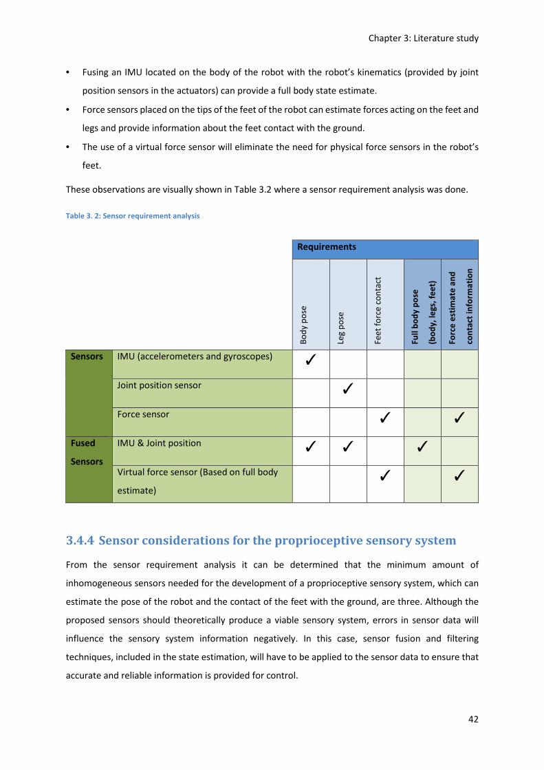
Chapter 3: Literature study
42
• Fusing an IMU located on the body of the robot with the robot’s kinematics (provided by joint
position sensors in the actuators) can provide a full body state estimate.
• Force sensors placed on the tips of the feet of the robot can estimate forces acting on the feet and
legs and provide information about the feet contact with the ground.
• The use of a virtual force sensor will eliminate the need for physical force sensors in the robot’s
feet.
These observations are visually shown in Table 3.2 where a sensor requirement analysis was done.
Table 3. 2: Sensor requirement analysis
Requirements
Bo
dy
po
se
Leg
po
se
Fee
t fo
rce
co
nta
ct
Fu
ll b
od
y p
ose
(bo
dy
, le
gs,
fe
et)
Fo
rce
est
ima
te a
nd
con
tact
in
form
ati
on
Sensors IMU (accelerometers and gyroscopes) ✓
Joint position sensor ✓
Force sensor ✓ ✓
Fused
Sensors
IMU & Joint position ✓ ✓ ✓
Virtual force sensor (Based on full body
estimate)
✓ ✓
3.4.4 Sensor considerations for the proprioceptive sensory system
From the sensor requirement analysis it can be determined that the minimum amount of
inhomogeneous sensors needed for the development of a proprioceptive sensory system, which can
estimate the pose of the robot and the contact of the feet with the ground, are three. Although the
proposed sensors should theoretically produce a viable sensory system, errors in sensor data will
influence the sensory system information negatively. In this case, sensor fusion and filtering
techniques, included in the state estimation, will have to be applied to the sensor data to ensure that
accurate and reliable information is provided for control.

Chapter 3: Literature study
43
It is therefore necessary to investigate commercially available sensors that apply to this study in order
to identify their advantages and more importantly, their disadvantages. The specification
considerations related to the sensors should also be identified to ensure the optimal sensors are
chosen to be integrated into the sensory system.
3.4.4.1 General considerations
The following specifications need to be considered in the designing phase of this study regarding the
sensor choices:
o Weight: In order to ensure the robot still has a high payload capability after the electronic
hardware for the sensory system has been integrated, the sensors should be as light as possible.
o Size: The size of the sensors should be of such nature that they can be integrated onto the platform
with ease.
o Power requirements: The supply voltage and current needed by the sensors should be considered
to avoid unnecessary power scaling or usage in the electronic design. The need for power scaling
introduces more components and unnecessary power consumption.
o Sensor models: Specific sensor noises should be investigated to provide adequate sensors models
to increase the accuracy of state estimation.
3.4.4.2 Joint position sensors
The PhantomX hexapod platform requires the use of the AX-12A or AX-18A Dynamixel servo actuators.
These actuators provide position feedback with the use of a potentiometer. Resistive potentiometers
have many advantages when used as position sensors. Resistive sensors are typically low in cost,
commonly available and easy to implement. Drawbacks associated with potentiometers include:
noticeable mechanical load, need to be physically connected to the object, subject to wear, and the
friction and applied voltage causes heating of the potentiometer.
3.4.4.3 IMU
The development of low-cost (less than $3000) IMUs such as micro electro mechanical systems
(MEMS), has increased their implementation in applications dramatically. MEMS also hold other
advantages such as small physical size, light weight and low power usage. These advantages makes
MEMS IMUs popular in robotic applications. Unfortunately, compared to the higher grade, expensive
IMUs, they exhibit larger measurement errors like scale factor drifts, turn-on and in-run biases and
noise [66], [67].

Chapter 3: Literature study
44
COTS IMUs that can be used for attitude estimation and navigation consists of accelerometers, which
measure linear acceleration, and angular rate sensors (gyroscopes). These two types of sensors are
used together to complement each other and provide more accurate estimates. The angular rate
sensors are subject to drift errors caused by bias errors and they perform well in a high frequency
range but are not accurate in a low frequency range. In contrast, the accelerometer sensors are not
subject to drift and they perform well in a low frequency range but are not accurate in a high frequency
range.
The errors produced by inertial sensors can be either deterministic (systematic) or random (dynamic).
Bias and scale factor errors that remain constant and are caused by external factors, such as
temperature, are deterministic. These errors are usually eliminated with the factory calibration done
by the IMU developer. Because low-cost MEMS sensors have larger systematic errors compared to
high cost IMUs, they need to be calibrated more frequently [67]. Most IMU distributers provide clients
with the service of recalibrating their IMU sensors.
Random errors in inertial sensor data are caused by random noise in the sensor signals. Over time
these random noise lead to drift in the bias or scale factor. Both a high frequency and low frequency
component is found in random noise [67]. The high frequency component is characterized by white
noise and is usually eliminated by a wavelet de-noising algorithm [68]. The low frequency component
has correlated noise characteristics that causes slow drifting and scale factor errors. These errors are
modelled by processes such as random walk or constant, Gaussian Markov and Auto Regressive
models [67]. These processes usually involve the use of the noise autocorrelation or Allan variance
function in order to obtain the first-order Gaussian Markov model [67].
Bloesch et al. [2] modelled the bias terms as Brownian motions where their derivatives can be
represented by white Gaussian noise. They specify the noise terms by the corresponding covariance
parameters that can be evaluated by examining the Allan variances. However, Bhatt et al. [67] state
that traditional approaches (applied to high-cost IMUs) like the Gauss Markov model and Allan
variance method is unsatisfactory for modelling random errors of MEMS sensors. Gebre-Egziabher
[69] advises that care should be taken when applying the Allan variance method to low-cost inertial
sensors. The Allan variance plots for low-cost sensors have correlated error slopes that are not
necessarily equal to one of the standard error sources represented by the Allan variance slopes [69].
Noureldin et al. [36], [70] modelled MEMS errors with an artificial intelligence approach that utilizes
Neural Networks. This approach proved to perform better than the conventional techniques but Bhatt
et al. [67] state that it suffers from poor generalisation capabilities and that it deteriorates after a

Chapter 3: Literature study
45
short time. The approach is also limited for real-time implementations. As a solution to this, Bhatt et
al. [67] proposes an enhanced Nu-Support Vector Regression technique in order to model the random
MEMS sensor errors.
It is important to note that the quantities provided by the sensors do not directly provide the
information that one might always want. For example, the angular rate needs to be integrated once
to provide the attitude, and to determine position, the acceleration has to be integrated twice. This
implies that an error in the acceleration measurement will cause a linear growing error in the velocity
calculation and an exponentially growing error in the position calculation. The errors in measurements
add up over time, which make the calculated values unusable [67]. For this reason Chao et al. [66]
states that an IMUs’ estimation accuracy heavily relays on the sensor fusion algorithm it uses.
In order to further minimize these errors it is important to consider IMUs that have aiding sensors
included. Aiding sensors are sensors that can provide other independent estimates of the information
that one needs from an IMU. The most common aiding sensors found in IMUs are a GPS and a
magnetometer. Another type of sensor that is commonly found in IMUs is a temperature sensor.
Temperature sensors are used in the factory calibration of the units to eliminate any errors in the data
estimates that are caused by temperature differences.
The following has to be considered in order to evaluate and choose a suitable IMU for the hexapod
sensory system:
• Internal sensors: The IMU needs at least a 3-axis accelerometer, a 3-axis gyroscope as well as a 3-
axis magnetometer (as a proprioceptive aiding sensor).
• Output data: The IMU should provide acceleration, angular rate and magnetic field data. Other
information such as the velocity, Euler angles, quaternion and rotation matrix will also be
beneficial but can be calculated from the acceleration, angular rate and magnetic field data as
needed for this study.
• Mechanical sensitivity: The IMU has to have low vibration and shock sensitivity in any direction to
keep the noise in the sensor readings to a minimum.
• Axis misalignment: Axis misalignment is when the axes of sensor triads are not exactly orthogonal
to each other. This should be as small as possible as it will cause cross-axis sensitivity errors.
• Scale factor: The scale factor is the ratio of the change in the output over the change in the
intended input to be measured.

Chapter 3: Literature study
46
3.4.4.4 Force sensors
A wide range of different types of force sensors that work in different ways exists. In the robotics field,
tactile force sensors are most commonly used in feet and finger tips to detect forces [71]. Tactile force
sensors are force transducers that are very popular as they are very thin. The most common, low-cost
tactile force sensors are force sensing resistors (FSR).
The following is suggested as desirable characteristics for tactile sensors [71]:
• The entire sensory area should be in contact when a force is applied (single-point contact). A
sensor with a small sensory area is thus beneficial.
• The sensitivity range that is determined by the sensors’ physical characteristics should be
considered. The typical sensitivity range that will be appropriate for this study are for example 0-
1 kg (0-10 N)
• The sensitivity due to the manner of application of the sensor should also be considered. This is
for example a barrier between the sensors and the contact object.
• A sensor bandwidth of 100 Hz minimum.
• The hysteresis and drift parameters should be as low as possible to avoid errors in feedback.
3.5 Conclusion
From the literature study conducted, a trade-off study was completed between different commercially
available hexapod platforms. As a result, the PhantomX Mark II hexapod robot kit was chosen to serve
as a platform for this study. This platform has a high payload capability, provides joint-angle feedback
and can easily be modified to include hardware such as sensors. For the state estimation of the robot,
a kinematic model will have to be derived. However, no measurement information regarding the robot
design is made available. This is seen as the main challenge presented with the use of the PhantomX
Mark II platform. Measurements will have to be taken from the physical platform to compute a
computer-aided model of the robot. The derivation of the platform’s kinematic model will be
discussed in Chapter 4.
Through an in-depth literature study that investigated state estimation approaches applied to legged
robots, an EKF framework, presented by Bloesch et al. [2], was chosen to be implemented for the state
estimation of the hexapod. Even though Bloesch et al. [2] only tested the filter on a quadruped, it is
stated that their EKF can be implemented on various kinds of legged robots. The framework provides
estimates regarding the position, velocity and quaternion of the centre of the robot body as well as

Chapter 3: Literature study
47
the positions of the robot’s feet contact points. Bias estimations regarding the IMU measurements are
also provided. The EKF presented not only provides all the information that is necessary for stability
control of the robot, it can also be interpreted as a SLAM algorithm. The EKF also allows expansion by
including further sensory measurements and can handle unknown environments and arbitrary
locomotion gaits. The derivation of the EKF for the hexapod platform will be discussed in Chapter 6.
The chapter concludes by identifying specific types of proprioceptive sensors needed for the
platform’s sensory system. These sensor types were chosen in such a manner to implement the state
estimation of the robot but also to allow future work on the platform and possible improvements to
the state estimation. Specific requirements that need to be considered when acquiring the sensors for
the sensory system were also discussed. The sensory devices chosen for this study as well as the
derivation of their measurement models will be discussed in Chapter 5.

Chapter 4: Kinematic model
48
Chapter 4: Kinematic model
“The most important thing is to keep the most important thing
the most important thing.”
~ From ‘Foundation design’, by Coduto, Donald P.
4.1 Introduction
The methodology followed to derive the kinematic model of the hexapod robot platform will be
discussed in this chapter. The kinematic model will specifically describe the forward kinematics of the
robot. This means that given a set of joint angles, the solution of the kinematic model will give the
position and orientation of the feet relative to a base frame on the body of the robot (body coordinate
frame). Since all of the legs of the hexapod robot are physically the same, it is possible to simplify the
derivation of the robot’s kinematic model by first deriving the kinematic model for one leg. After
modelling one leg of the hexapod, the entire robot can be modelled by transforming the leg kinematics
into the body coordinate frame. Lastly, the kinematic measurement model is derived for the state
estimation of the robot.
4.2 Background
In this section background is discussed regarding the descriptions and their operators used to specify
attributes that will be needed to derive the kinematic model of the hexapod robot. The description of
positions, orientations and frames will be considered along with their corresponding operators,
namely translation, rotation and transformation. Introduction to robotics: mechanics and control was
used for the theory of the kinematics [72].
4.2.1 Position
By establishing a coordinate system, the location of any point in space can be determined with a 3 ×1position vector. Let the point, d§ , be represented by a position vector located in coordinate
system,{©}, and let the individual elements of the vector be represented by !«, !¬ and ! such that
d§ = ®!«!¬!¯. (4. 1)

Chapter 4: Kinematic model
49
Fig. 4.1 shows a coordinate system{©} with three mutually orthogonal unit vectors, o_§, r_§ and _§,
and a point d§ , representing a vector locating a position in space.
Figure 4. 1: Position vector relative to a coordinate frame.
Translation can be defined as an operator that moves a point, dA§ , a finite distance along a given
vector direction provided by vector, Y§ . The result of the translation operator is a new point d�§ ,
shown in Fig. 4.2 and given by
d�§ = dA§ + Y§ . (4. 2)
Figure 4. 2: Translation of a point.
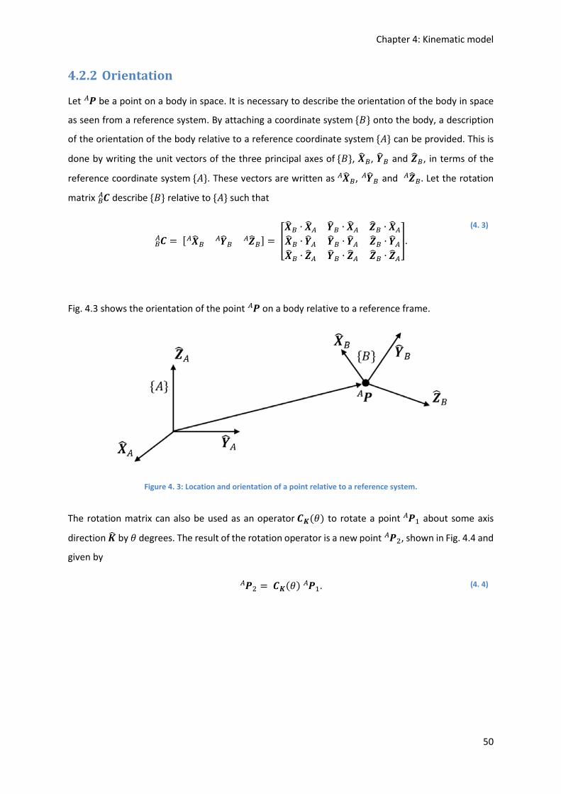
Chapter 4: Kinematic model
50
4.2.2 Orientation
Let d§ be a point on a body in space. It is necessary to describe the orientation of the body in space
as seen from a reference system. By attaching a coordinate system{°} onto the body, a description
of the orientation of the body relative to a reference coordinate system{©} can be provided. This is
done by writing the unit vectors of the three principal axes of{°}, o_±, r_± and _±, in terms of the
reference coordinate system{©}. These vectors are written as o_§ ±, r_§ ± and _§ ±. Let the rotation
matrix T±§ describe{°} relative to{©} such that
T±§ = ² o_§ ± r_§ ± _§ ±³ = ´o_± ∙ o_§ r_± ∙ o_§ _± ∙ o_§o_± ∙ r_§ r_± ∙ r_§ _± ∙ r_§o_± ∙ _§ r_± ∙ _§ _± ∙ _§µ. (4. 3)
Fig. 4.3 shows the orientation of the point d§ on a body relative to a reference frame.
Figure 4. 3: Location and orientation of a point relative to a reference system.
The rotation matrix can also be used as an operatorT^(}) to rotate a point dA§ about some axis
direction _̂ by} degrees. The result of the rotation operator is a new point d�§ , shown in Fig. 4.4 and
given by
d�§ =T^(}) dA§ . (4. 4)

Chapter 4: Kinematic model
51
Figure 4. 4: Rotation of a point about the _axis by θ degrees ( d¶· = T(�) d¸· ).
4.2.3 Frames
A robot can physically be described as a system of rigid bodies that are connected with joints. For each
rigid body, its orientation together with its position in space is defined as its pose [31]. In order to
determine the pose of a rigid body in space, we define an entity called a frame as a set of four vectors
consisting of orientation and position [72]. A frame is therefore a coordinate system that gives the
orientation as well as the position vector that locates the frame’s origin relative to some other frame.
With regard to this study, a right-handed frame is defined as a frame with a three dimensional
coordinate system in which the axes satisfy the right-hand rule. The right-hand rule is described as
follows. For the right hand, with the thumb and index finger (first finger) stretched out, the second
finger bend in to form a90° angle relative to the index finger, and the third and fourth fingers curled
in towards the palm, the right-hand rule states that:
- The orientation of the thumb define the positive t-axis, the orientation of the index finger
define the positive p-axis, and the orientation of the second finger define the positive s-axis.
- The curl direction of the third and fourth finger indicate the positive rotation along the t-axis
and define that the positive rotation along any of the axes are anti-clockwise.
Fig. 4.5 shows the right-hand rule.

Chapter 4: Kinematic model
52
Figure 4. 5: Right-hand rule.
For this study, the symbol : is defined to represent the body coordinate frame (on the robot) and the
symbol $ is defined to represent the inertial coordinate frame (non-accelerating reference in space).
The relationship between the body coordinate frame : and the inertial coordinate frame$ can be
described by the rotation matrix T±¹ and the position vector, d¹ ±º»¼, locating the origin of frame :
relative to frame $.
: = { T±¹ , d¹ ±º»¼}. (4. 5)
Related to the descriptor frame, the matrix operator transformation,m, can be defined. The
transformation operator rotates and translates a vector dA§ . The result of the transformation
operator is a new vector d�§ , given by
d�§ = m dA§ . (4. 6)
The transformation operator can also be used to rotate and translate a vector point d± in frame{°} into frame {½}, written as
d¹ = m±¹ d± . (4. 7)
4.3 Robotic platform
The PhantomX® [51] hexapod robot platform is used as a base platform for this study. This specific
platform is chosen based on the results of the trade-off study conducted in the literature study with
regards to different commercially available hexapod platforms. Since the robot is only a prototype, no
mechanical design was implemented with regard to the integration of the different components onto
the platform. The extra components needed for this study were simply placed on the robot in an
organized manner, distributing their weight equally throughout the robot body. This section is merely

Chapter 4: Kinematic model
53
provided as context to the reader with regard to the derivation of the kinematic model and the
location of the sensors. Fig. 4.6 is a photo of the final robot prototype as used in this study.
Figure 4. 6: Robot prototype with integrated sensors.
The following components were integrated onto the PhantomX® robot platform:
- Six FlexiForce® A201 force sensors, one per foot [73].
- One MicroStrain 3DM-GX3®-25 IMU [74].
- One UDOO (single-board computer) [75].
- One Lithium Polymer battery.
An in-depth discussion on the specific integrated sensors can be found in Chapter 5. The internal
coordinate frame of the IMU is used as the body coordinate frame for the robot in all calculations. The
IMU is mounted on top of a 2 mm thick Perspex plate, with the t-axis of the IMU aligning with the
middle of the robot body. Fig. 4.7 shows the location of the IMU on the robot as well as the location
of the IMU’s internal coordinate frame. The exact dimensions of the location of the origin of the
internal coordinate frame inside the IMU can be found in its mounting diagram [76].

Chapter 4: Kinematic model
54
Figure 4. 7: Location of the IMU on the robot platform.
Each of the servo motors on the robot has been assigned with an ID. Fig. 4.8 shows a top view of the
robot indicating the specific servo motors and their corresponding ID’s for each leg. Throughout this
study, this figure will be used as a reference to identify specific servo motors.
Figure 4. 8: Top view of robot with servo motor ID's.
4.4 Kinematic model for a robot leg
The PhantomX® hexapod robot has six legs. Each leg can be characterised by four rigid bodies, the
base, coxa, femur and tibia. Each rigid body can mathematically be presented as a ¾.¿/. Servo motors
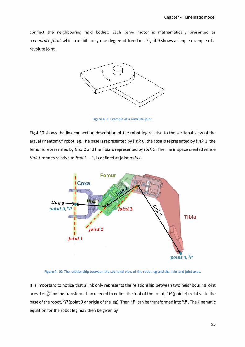
Chapter 4: Kinematic model
55
connect the neighbouring rigid bodies. Each servo motor is mathematically presented as
aÀ�Á¾Ã<�ÄÂ.¿< which exhibits only one degree of freedom. Fig. 4.9 shows a simple example of a
revolute joint.
Figure 4. 9: Example of a revolute joint.
Fig.4.10 shows the link-connection description of the robot leg relative to the sectional view of the
actual PhantomX® robot leg. The base is represented by ¾.¿/0, the coxa is represented by ¾.¿/1, the
femur is represented by ¾.¿/2 and the tibia is represented by ¾.¿/3. The line in space created where ¾.¿/. rotates relative to ¾.¿/. − 1, is defined as joint � .Å ..
Figure 4. 10: The relationship between the sectional view of the robot leg and the links and joint axes.
It is important to notice that a link only represents the relationship between two neighbouring joint
axes. Let mÆÇ be the transformation needed to define the foot of the robot, dÆ (point 4) relative to the
base of the robot, dÇ (point 0 or origin of the leg). Then dÆ can be transformed into dÇ . The kinematic
equation for the robot leg may then be given by

Chapter 4: Kinematic model
56
dÇ = mÆÇ dÆ . (4. 8)
4.4.1 Derivation of link parameters and affixing frames to links
In order to derive the kinematic model for the robot leg, the Denavit-Hartenberg notation is used [72].
In order to describe the robot leg kinematically, four parameters, namely; link length, link twist, link
offset and joint angle will now be defined and assigned to each link. The assignment of the link
parameters is shown in Fig.4.11.
Figure 4. 11: Example of allocation of the four link parameters.
Let the¾.¿/¾�¿'<ℎ, ��QAof¾.¿/. − 1 be defined as the length of a line that exists mutually
perpendicular to both� .Å. and� .Å. − 1 . The line that defines the link length will always exist and,
except in the case where both axes are parallel, will always be unique. It is now possible to construct
a plane with its normal, the line defining the link length. By projecting the � .Å. − 1 and the� .Å. onto this plane, the angle existing between them can be measured. Let the ¾.¿/<È.Å<v�QA of¾.¿/. −1, be defined as the angle measured about ��QA from� .Å. − 1 to� .Å.. This measurement should
be done using the right-hand principle.
For any two¾.¿/Å. − 1 and ., that are connected, there exists a common joint� .Å. between them.
Let the ¾.¿/Â))Å�<��, be defined as the signed distance between the intersection of ��QA with the
axis ofÄÂ.¿<., and the intersection of �� with the axis ofÄÂ.¿<.. Let the�¿'¾�}�, be defined as the
angle measured about the common ÄÂ.¿<� .Å., between the connected¾.¿/Å. − 1 and .. For a
revolute joint, the joint angle is a variable.

Chapter 4: Kinematic model
57
The relationship between any two axes in space can be defined by only the link length and the link
twist. The link offset and joint angle are used to specify how links are connected to each other. In
order to define the location of neighbouring links relatively to each other, a frame will be attached to
each link. The following convention is used to attach a frame to each link:
The number of a specific frame is in accordance with the link it is attached to. Therefore, )À�É�{. −1} is attached to¾.¿/. − 1, )À�É�{.} is attached to ¾.¿/., and so on. The following method is used
to locate frames on the links [72]:
• For )À�É�{.}, the p-axis is called pq�, the s-axis is called sq� and the t-axis is called tu�. • The origin c�, of frame {.} is located where the line defining the ¾.¿/¾�¿'<ℎ�� intersects the ÄÂ.¿<. axis perpendicular.
• tu� is coincident with ÄÂ.¿<� .Å.. • pq� is located on �� pointing from ÄÂ.¿<. towards ÄÂ.¿<. + 1. When �� = 0, pq� is normal to the
plane of both tu� and tu�@A.
• v� is measured about pq� according to the right-hand principle.
• The )À�É�{.} is completed by forming sq� with the right-hand rule.
Fig.4.12 shows the parameter and link-frame assignments for the robot leg. XÀ�É�{0} is attached to
the base of the robot leg (body of the robot or ¾.¿/0). XÀ�É�{0} never moves and can therefore be
seen as the reference frame. XÀ�É�{0} is also chosen to coincide with )À�É�{1} with tuÇ along � .Å1. This results in �Ç = 0, vÇ = 0 and �A = 0, since ÄÂ.¿<1 is revolute. For)À�É�{4}, pqÆ is
chosen to align with pqK so that }Æ = 0. The origin cÆ, of )À�É�{4} is chosen where �Æ = 0.
Table 4.1 provides a summary of the link parameter values of the PhantomX® hexapod robot leg:
Table 4. 1: Link Parameter Values.
. v�QA[°] ��QA[m] ��[m] }�[°] 1 0 0 0 }A
2 90 0.0520 0 }�
3 0 0.0662 0 }K
4 0 0.1389 0 0

Chapter 4: Kinematic model
58
Figure 4. 12: Parameter and link-frame assignment from the robot Leg.
4.4.2 Derivation of the link transformations
With the implementation of a frame for each link, we have divided the kinematic problem into four
subproblems. These subproblems represent the transformations between the neighbouring frames,
namely mAÇ , m�A , mK� and mÆK . By using the four link parameters defined, one can further divide each
subproblem into four. This can be used to derive a general transformation that describes the
relationships between neighbouring frames:
Let m��QA represent the transformation that defines )À�É�{.} relative to )À�É�{. − 1}. This
transformation will always be a function of the four link parameters defined with one of them being a
variable and the other three fixed in value. The transformation that transform d� , a point defined in )À�É�{.} to d�QA , the same point described in )À�É�{. − 1} can be represented as
Ê d�QA1 Ë = m��QA Ê d�1 Ë. (4. 9)
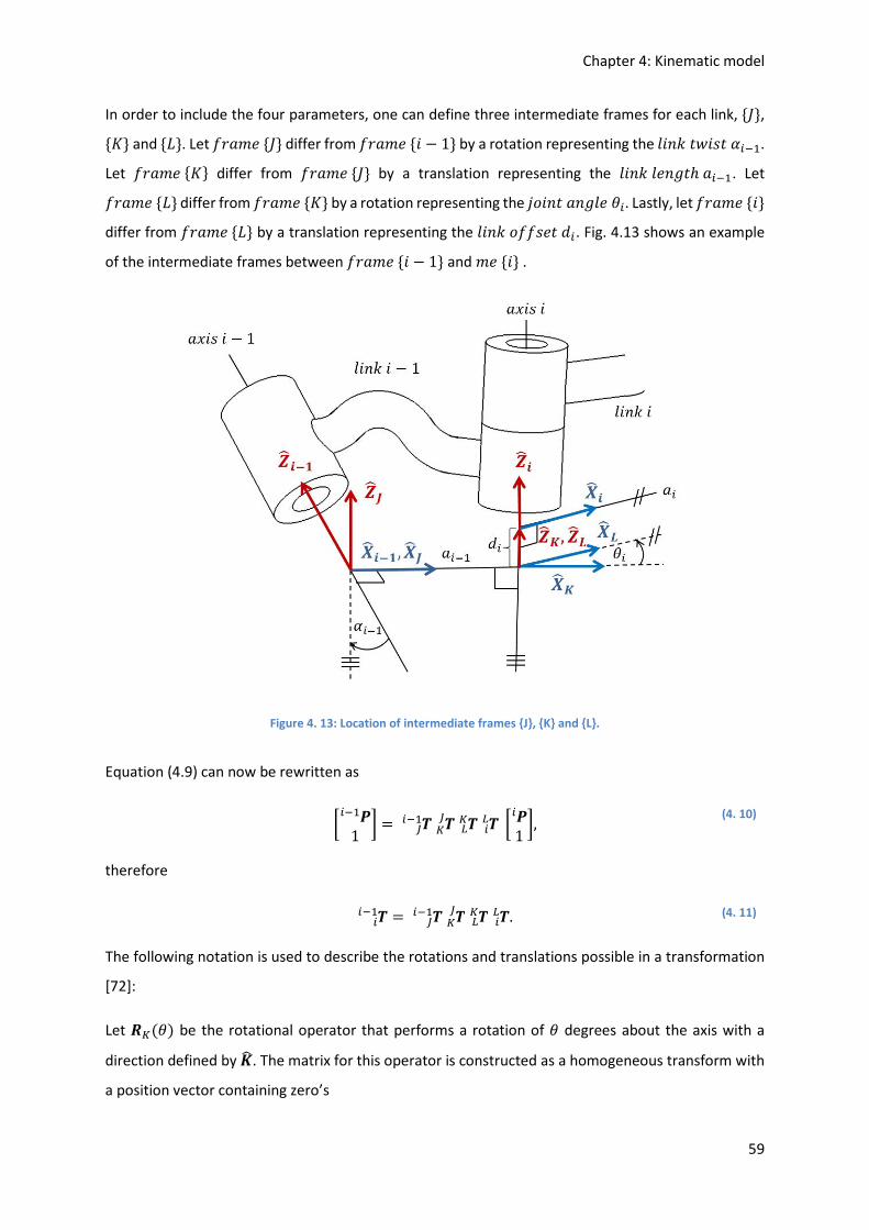
Chapter 4: Kinematic model
59
In order to include the four parameters, one can define three intermediate frames for each link, {Ì}, {Í} and {a}. Let )À�É�{Ì} differ from )À�É�{. − 1} by a rotation representing the ¾.¿/<È.Å<v�QA.
Let )À�É�{Í} differ from )À�É�{Ì} by a translation representing the ¾.¿/¾�¿'<ℎ��QA. Let )À�É�{a} differ from )À�É�{Í} by a rotation representing the ÄÂ.¿<�¿'¾�}�. Lastly, let )À�É�{.} differ from )À�É�{a} by a translation representing the ¾.¿/Â))Å�<��. Fig. 4.13 shows an example
of the intermediate frames between )À�É�{. − 1} and É�{.} .
Figure 4. 13: Location of intermediate frames {J}, {K} and {L}.
Equation (4.9) can now be rewritten as
Ê d�QA1 Ë = mÎ�QA mÏÎ mÐÏ m�Ð Ê d�1 Ë, (4. 10)
therefore
m��QA = mÎ�QA mÏÎ mÐÏ m�Ð . (4. 11)
The following notation is used to describe the rotations and translations possible in a transformation
[72]:
Let iÏ(}) be the rotational operator that performs a rotation of } degrees about the axis with a
direction defined by _̂ . The matrix for this operator is constructed as a homogeneous transform with
a position vector containing zero’s

Chapter 4: Kinematic model
60
iÏ(}) = ´[TÏ(})]0 0 0
0001µ, (4. 12)
where [TÏ] is the standard 3 × 3 rotation matrix used to rotate a vector around the axis determined
by _̂ .
Let ÑY(Z) represent a translation along the vector direction defined by Y with a signed magnitude of Z. The matrix for this operator is a homogeneous transform with the following form:
ÑY(Z) = Ò1 0 00 1 00 0 1Z«Z¬Z0 0 0 1 Ó, (4. 13)
where, Z =ÔZ«� +Z¬� +Z�. Z«, Z¬ and Z are the components of the translation vector Y.
Equation (4.11) can be simplified by considering each of the transformations individually. The
transformation m�QA is a rotation of angle v�QA about the o_ axis and can therefore be reduced
toiÕ(v�QA). The transformation mÏÎ is a translation of length ��QA along the o_ axis and can therefore
be reduced to ÑÕ(��QA). The transformation mÐÏ is a rotation about the _ axis by an angle of }� and
can therefore be reduced to iÖ(}�). Lastly, m�Ð is a translation along the _ axis of magnitude �� and
can therefore be reduced to ÑÖ(�� ). Equation (4.11) can now be written as
m��QA =iÕ(v�QA)ÑÕ(��QA)iÖ(}�)ÑÖ(�� ). (4. 14)
By expanding (4.14), the general form for the transformation between neighbouring links is given by
m =��QA Ò cos(}�)sin(}�) cos(v�QA)sin(}�) sin(v�QA)0−sin(}�)cos(}�)cos(v�QA)cos(}�) sin(v�QA)0
0−sin(v�QA)cos(v�QA)0��QA−sin(v�QA)��cos(v�QA) ��1 Ó. (4. 15)
The PhantomX® hexapod robot leg kinematic model can now be derived using
Ê dÇ1 Ë = mAÇ m�A m mÆKK� Ê dÆ 1 Ë. (4. 16)
Using link parameters as described in Table 4.1 together with (4.15), the respective transformation
matrices are given as follows
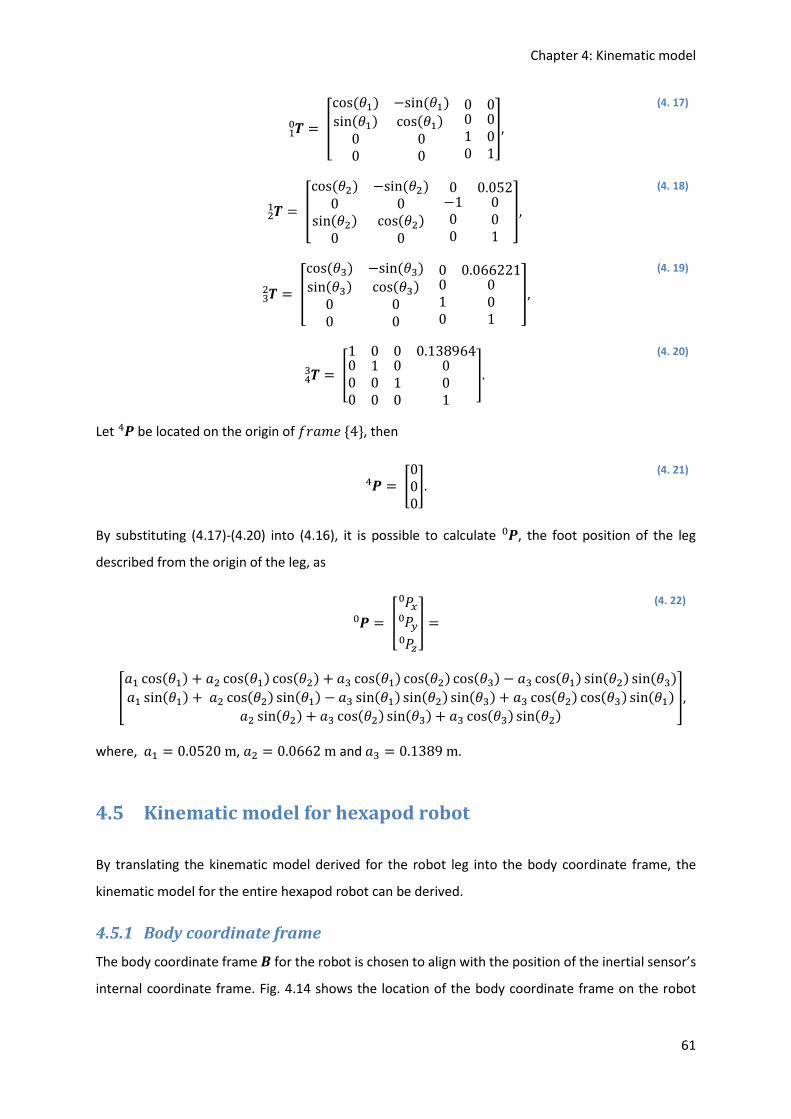
Chapter 4: Kinematic model
61
mAÇ = Òcos(}A)sin(}A)00−sin(}A)cos(}A)00
00100001Ó,
(4. 17)
m�A = Òcos(}�)0sin(}�)0−sin(}�)0cos(}�)0
0−1000.052001 Ó, (4. 18)
mK� = Òcos(}K)sin(}K)00−sin(}K)cos(}K)00
00100.066221001 Ó, (4. 19)
mÆK = ´10000100
00100.138964001 µ. (4. 20)
Let dÆ be located on the origin of )À�É�{4}, then
dÆ = ®000¯. (4. 21)
By substituting (4.17)-(4.20) into (4.16), it is possible to calculate dÇ , the foot position of the leg
described from the origin of the leg, as
dÇ = ´ ØÇ «ØÇ ¬ØÇ µ =
(4. 22)
´�A cos(}A) + �� cos(}A) cos(}�) + �K cos(}A) cos(}�) cos(}K) − �K cos(}A) sin(}�) sin(}K)�A sin(}A) +�� cos(}�) sin(}A) − �K sin(}A) sin(}�) sin(}K) + �K cos(}�) cos(}K) sin(}A)�� sin(}�) + �K cos(}�) sin(}K) + �K cos(}K) sin(}�) µ, where, �A = 0.0520m, �� = 0.0662m and �K = 0.1389m.
4.5 Kinematic model for hexapod robot
By translating the kinematic model derived for the robot leg into the body coordinate frame, the
kinematic model for the entire hexapod robot can be derived.
4.5.1 Body coordinate frame
The body coordinate frame : for the robot is chosen to align with the position of the inertial sensor’s
internal coordinate frame. Fig. 4.14 shows the location of the body coordinate frame on the robot

Chapter 4: Kinematic model
62
body as well as the measurements defining the relationship between the body coordinate frame and
the origin of each leg.
Figure 4. 14: Relationship between the body coordinate frame and origin of legs.
By considering Fig. 4.14, the kinematic model of a single leg can be transformed into the robot
kinematic model.
4.5.2 Robot kinematic model
Let d�Ç , represent the foot position of leg . as seen from the origin of the leg .. That means, d�Ç is the
result given by the leg kinematic model for leg .. From Fig. 4.14 it is clear that for each leg, the leg
kinematic model will have to undergo a rotation about the t-axis (TÖ(x�)), as well as translations in
all axes (!« , !¬, !). This transformation, needed to describe the foot position of leg . in terms of the
body coordinate frame, is represented by
Ê d�±1 Ë = Ò®TÖ(x�) ¯
0 0 0®!«!¬!¯1 Ó Ê d�Ç1 Ë. (4. 23)
Table 4.2 provides the parameter values used in (4.23) to derive the robot kinematic model.

Chapter 4: Kinematic model
63
Table 4. 2: Measurements used to derive the robot kinematic model.
. x[°] !« [m] ( � = 0.0605 J = 0.1005) !¬[É] (Ù = 0.1206) !²É³ (M = 0.0265)
1 45 � Ù M
2 135 − � Ù M
3 0 J 0 M
4 180 − J 0 M
5 315 � −Ù M
6 225 − � −Ù M
By substituting the translation values as given in Table 4.2 into (4.23), one can derive the kinematic
model of the robot in order to determine the foot positions with respect to the body coordinate frame.
For better readability the robot’s kinematic equations,012�(�), are given separately for each leg .. Here, � = ²}A, }�, }K³as defined in (4.22). Furthermore, the symbols as defined in Table 4.2 and the
measurement quantities as defined in (4.22) are used.
Leg one:
012A(�) = ² dA± ³ = ÚÛÛÛÛÜ � +
(2Ç.Ý × d«Þ)Ç2 −(2Ç.Ý × d¬Þ)Ç2Ù + (2Ç.Ý × d«Þ)Ç2 +(2Ç.Ý × d¬Þ)Ç2dÞ + MÇ ßààààá.
(4. 24)
Leg two:
012�(�) = ² d�± ³ = ÚÛÛÛÛÜ− � −
(2Ç.Ý × d«â)Ç2 −(2Ç.Ý × d¬â)Ç2Ù + (2Ç.Ý × d«â)Ç2 +(2Ç.Ý × d¬â)Ç2dâ + MÇ ßààààá.
(4. 25)
Leg three:
012K(�) = ² dK± ³ = Ò d«ã + JÇ d¬ã Çdã + MÇÓ. (4. 26)

Chapter 4: Kinematic model
64
Leg four:
012Æ(�) = [ dƱ ] = Ò− d«ä − JÇ− d¬äÇdä + MÇÓ. (4. 27)
Leg five:
012Ý(�) = [ dݱ ] = ÚÛÛÛÛÜ � +
(2Ç.Ý × d«å)Ç2 +(2Ç.Ý × d¬å)Ç2−Ù − (2Ç.Ý × d«å)Ç2 +(2Ç.Ý × d¬å)Ç2då + MÇ ßààààá.
(4. 28)
Leg six:
012æ(�) = ² dæ± ³ = ÚÛÛÛÛÜ− � −
(2Ç.Ý × d«ç)Ç2 +(2Ç.Ý × d¬ç)Ç2−Ù − (2Ç.Ý × d«ç)Ç2 −(2Ç.Ý × d¬ç)Ç2dæ + MÇ ßààààá.
(4. 29)
4.6 Kinematic measurement model
The kinematic model 012�(�) for leg . of the robot computes the location of each foot with respect
to the body coordinate frame. However, for the state estimation of the robot, errors have to be taken
into account that might affect the accuracy of the kinematic model. These can include erroneous
calibration of the position sensors and errors in the kinematic model such as inaccuracies in
measurements of the rigid bodies. 9� is defined as a vector pointing from the body coordinate frame
to the contact point of foot .. For the errors affecting the kinematic model, following Bloesch et al.[2],
the discrete Gaussian noise terms 23,� is added in the model:
9� = 012�(�) + 23,� . (4. 30)
Let i3 be the covariance matrix for the noise 23,�.
4.7 Conclusion
In this chapter the kinematic model for the robot platform was derived. Background information
regarding descriptions and specific operators used in this study was firstly discussed. Important

Chapter 4: Kinematic model
65
information about the robot platform was also given. This included the servo motor ID locations that
are referenced throughout this study. A photo of the final robot platform was also provided along with
a list of the components integrated onto the original PhantomX® platform.
The derivation of the robot kinematic model was done in a two-step process. Firstly, a model was
derived for a leg of the robot. Here, link parameters were derived and frames were affixed to these
links. The derivation of the link transformations were also completed. Secondly, the leg kinematic
model was used to derive the final robot kinematic model. This was done by translating the leg
kinematic model into the body coordinate frame for each leg.
This chapter concluded with a discussion regarding the kinematic measurement model. The sensory
devices chosen for this study to be integrated onto the robot platform will now be discussed. For each
of the sensory devices chosen, a measurement model will be derived. These measurement models
along with the kinematic measurement model derived in this chapter will be used for the state
estimation of the robot.

Chapter 5: Sensory system
66
Chapter 5: Sensory system
“Remember that all models are wrong; the practical question
is how wrong do they have to be to not be useful.”
~ George Edward Pelham Box
5.1 Introduction
In this chapter the sensory system developed for this study is discussed. The sensory devices chosen
for this study are firstly discussed. Some information regarding the implementation of the sensory
measurements are also given. The method followed to acquire the sensor data is then discussed. The
chapter concludes with the derivation of the measurement models to describe the noise processes of
the sensor measurements. Standard deviation quantities are also assigned to the noise processes.
5.2 Sensory devices
This section discusses the specific sensory devices chosen for the proprioceptive sensory system used
in this study. These sensory devices were chosen to comply with the requirements as set out in
Chapter 3.
5.2.1 Joint position Sensors
The PhantomX® [51] hexapod robot platform used in this study makes use of AX-12A Dynamixel servo
motors [77] with resistive potentiometers that provide joint position feedback. The joint position
feedback provide the angular positions for all the joints as needed by the kinematic model for the
robot. The AX-12A allows 0-300° of movement with a control and feedback range of 0-1023 bits.
An advantage specifically related to the Dynamixel servo design is that the potentiometer is placed on
the output shaft and not directly after the motor, i.e. before the gears. This means that any play
amongst the gear teeth that has a direct influence on the final movement is considered in the feedback
readings [71].
Research conducted by Tira-Thompson [78] shows that the Dynamixel AX-12A servo’s position
feedback regarding a target position is very accurate (0.36°) when under no load. As the load on the
servo increases the deflection from the target position increases. (Note that the position feedback
regarding the real shaft position is not influenced by added load on the servo.) According to research
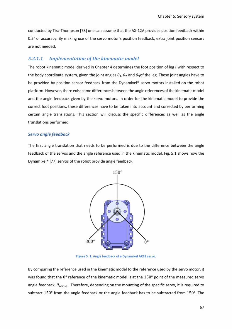
Chapter 5: Sensory system
67
conducted by Tira-Thompson [78] one can assume that the AX-12A provides position feedback within
0.5° of accuracy. By making use of the servo motor’s position feedback, extra joint position sensors
are not needed.
5.2.1.1 Implementation of the kinematic model
The robot kinematic model derived in Chapter 4 determines the foot position of leg . with respect to
the body coordinate system, given the joint angles }A, }�and }Kof the leg. These joint angles have to
be provided by position sensor feedback from the Dynamixel® servo motors installed on the robot
platform. However, there exist some differences between the angle references of the kinematic model
and the angle feedback given by the servo motors. In order for the kinematic model to provide the
correct foot positions, these differences have to be taken into account and corrected by performing
certain angle translations. This section will discuss the specific differences as well as the angle
translations performed.
Servo angle feedback
The first angle translation that needs to be performed is due to the difference between the angle
feedback of the servos and the angle reference used in the kinematic model. Fig. 5.1 shows how the
Dynamixel® [77] servos of the robot provide angle feedback.
Figure 5. 1: Angle feedback of a Dynamixel AX12 servo.
By comparing the reference used in the kinematic model to the reference used by the servo motor, it
was found that the 0° reference of the kinematic model is at the 150° point of the measured servo
angle feedback,}3~��� . Therefore, depending on the mounting of the specific servo, it is required to
subtract 150° from the angle feedback or the angle feedback has to be subtracted from150°. The

Chapter 5: Sensory system
68
translated servo position feedback, }����3���~�, is the result of this translation for the specific servo
motors:
For the servo motors with the following ID numbers: 1, 2, 4, 6, 7, 8, 10, 12, 13, 14, 16 and 18
}����3���~� = 150° − }3~���. (5. 1)
For the servo motors with the following ID numbers: 3, 5, 9, 11, 15 and 17
}����3���~� =}3~��� − 150°. (5. 2)
Leg structure
Each rigid body of the leg consists of a servo motor that is connected to one or more brackets. By
examining the femur and tibia of the robot leg, it is found that the servo motor for each does not align
with the mathematical link allocation given for the kinematic model. This is made clear in Fig. 5.2.
There exists a 13.09° difference between the servo motor of the femur and ¾.¿/2 and a 45.36° difference between the servo motor in the tibia and¾.¿/3.
Figure 5. 2: Relationship between the leg structure and link location.
The differences between the leg structure and the mathematical model used in the kinematic model
can be eliminated by the following translations:
For the servo motors with the following ID numbers: 3, 4, 9, 10, 15 and 16
} = }����3���~� + 13.09°. (5. 3)

Chapter 5: Sensory system
69
For the servo motors with the following ID numbers: 5, 6, 11, 12, 17 and 18
} = }����3���~� + 45.36° − 13.09°. (5. 4)
The combination of (5.1)-(5.4) defines the total degree translations needed in order to transform the
servo motor angle feedback to comply with the joint angles needed by the kinematic model:
For the servo motors with the following ID numbers: 1, 2, 7, 8, 13 and 14
}A = 150° −}3~���. (5. 5)
For the servo motors with the following ID numbers: 3, 9 and 15
}� =}3~��� − 136.91°. (5. 6)
For the servo motors with the following ID numbers: 4, 10 and 16
}� = 163.09° −}3~���. (5. 7)
For the servo motors with the following ID numbers: 5, 11 and 17
}K =}3~��� − 117.73°. (5. 8)
For the servo motors with the following ID numbers: 6, 12 and 18
}� = 182.27° −}3~���. (5. 9)
5.2.2 MicroStrain 3DM-GX3-25
The MicroStrain 3DM-GX3-25 miniature attitude heading reference system (AHRS) was chosen for this
study. It is a low cost, high-performance inertial sensor that can be applied in a wide range of
applications (e.g., inertial aiding of GPS, unmanned vehicle navigation, platform stabilization, robotic
control, personal tracking, etc.) [79]. The device utilises MEMS sensor technology and integrates a
triaxial accelerometer, a triaxial gyroscope, a triaxial magnetometer, five temperature sensors as well
as an on-board processor. The device weighs 18 grams and is 44mm× 24mm× 11mm in size. Fig.
5.3 shows a picture of the 3DM-GX3-25 sensor device.

Chapter 5: Sensory system
70
Figure 5. 3: MicroStrain 3DM-GX3-25 inertial sensor [79].
The 3DM-GX3-25 offers the following fully calibrated measurements for an operating temperature of −40°C to70°C: acceleration, angular rate, magnetic field, delta-theta and delta-velocity vectors,
Euler angles, rotation matrix and quaternion. It provides an attitude heading range of 360°/s about
all three axes with an accelerometer range of ±5g and a gyroscope range of±300°/s. The sensor
supports an USB 2.0 or RS232 interface and has a micro-DB9 connector. Its data output rate is up to 1000Hz with baud rate options of 115200 bps to 921600 bps. The sensor can be supplied with a
direct current supply of +3.2V to +16V and consumes 80mA@5V with USB. (The data sheet for
this device can be found in Appendix B.)
The measured acceleration quantity given by the IMU,$%&, is scaled into the physical unit of g-force
acceleration g, where1g = ' = 9.80665m/s�. The proper acceleration is therefore related to the
measured acceleration as follows
= ' × $%&. (5. 10)
The measured gravitational acceleration varies from the standard 9.80665m/s� depending on the
geographical location where the sensor is used. The following formula is used to determine the local
gravitational acceleration [80]:
'� = 9.780318(1 + 0.0053024 sin�(a) − 0.0000058 sin�(2a)) − 3.086 × 10Qæℎ, (5. 11)
where, '� is the locally measured acceleration of gravity [m/s�³, a is the latitude ²°³ and ℎ is the
altitude [m³ above sea level for the specific location. In order for (5.10) to provide the correct proper
acceleration, the locally measured gravitational acceleration needs to be deducted from the measured
acceleration, and replaced with the standard value of 9.80665m/s�. By using the rotation matrix T$%& provided by the IMU, one can redefine (5.10) as:
= ($%& × ') − (T$%& × *+) + (T$%& × *), (5. 12)

Chapter 5: Sensory system
71
where * is the standard gravity vector
* = ® 00−'¯, (5. 13)
and *+ is the local measured gravity vector
*+ = ® 00−'�¯. (5. 14)
For the state estimation of the robot the IMU is used to provide the proper acceleration and the
angular rateh of the robot’s main body. The relationship between the proper acceleration and the
absolute acceleration � is given by
The rotation matrix T is responsible for the rotation of coordinates represented in the inertial
coordinate frame $ into the body coordinate frame :.
5.2.3 Force Sensors
With regard to the state estimation for this study, Bloesch et al. [2] stated that they experienced a 10% drift in the estimated travelled distance of their robot which can be a result of fault-prone
contact detection. The foot contact detection will be used in the state estimation of the robot to define
the value of a specific noise parameter defined for a certain foothold (Chapter 6). The foot contact
state for any given leg with a known robot pose can be estimated by the robot’s kinematic model. Due
to the limited control of the robot platform at this stage of development, detecting the feet contact
states through the kinematic model will only be viable when the robot navigates on an even surface.
In order to minimise drift in our estimation and to provide a basis for future work, it was decided to
include force sensors on the robot platform to provide the foot contact information needed. The force
sensors are integrated into the hexapod’s feet. A201 type FlexiForce sensors [73], distributed by
Tekscan, were chosen for this study [73]. These sensors are ultra-thin, light in weight and flexible. The
FlexiForce sensor is a force sensing resistor, decreasing in resistance value as a force is being applied
to the sensing area. They can easily be included in a number of standard electronic circuit designs and
used as an analogue input, as needed by software. The specific model integrated onto the robot can
measure 0 to 100N and has a response time smaller than5ms. Fig. 5.4 shows a picture of the A201
sensor.
= T(� − *). (5. 15)

Chapter 5: Sensory system
72
Figure 5. 4: A201 FlexiForce sensor.
For this study the FlexiForce sensors will only be used as on-off devices indicating if the feet are in
contact with the ground or not. Each sensor was therefore integrated into a comparator circuit making
use of an operational amplifier to produce a high analogue voltage output when the foot has no
ground contact and a 0V analogue output when the foot has ground contact. See Appendix B for
physical information on the sensors as well as the electronic circuit used to integrate the sensors onto
the platform.
5.3 Sensory system data acquisition
This section discusses the data acquisition of the IMU, joint position sensors and the force sensors.
With regards to this study, the purpose of the sensory system is to provide the necessary
measurements needed for state estimation. For the state estimation of the robot, the following
sensory data needed to be collected: The position feedback from all 18 servo motors, ground contact
status from the force sensors, and acceleration, angular rate, time stamp and quaternion
measurements from the IMU.
5.3.1 Data Acquisition Frequency
Data acquisition frequency refers to the rate at which the data from the sensors is captured by the
sensory system. A sensor acquisition frequency of 20Hz was chosen experimentally. This is because
the movement of the robot became intermittent when servo position feedback was requested at
higher frequencies. It is important to note that this limitation is brought on by the restrictions in the
current control of the robot and can be improved with the development of the robot control in future
work.
For successful state estimation of the robot, a single leg movement should be shown in the sensor
data. Therefore, the sensor data acquisition speed should be faster than the robot moving a leg to a
new position and each contact position should be recorded. In order to validate that a data acquisition
speed of 20Hz is fast enough for state estimation of the robot, the robot was filmed with a high speed
camera to show the distance travelled by the robot at full speed every50ms. Fig. 5.5 illustrates four
frames captured by the high speed camera at 50ms intervals.

Chapter 5: Sensory system
73
Figure 5. 5: Robot Platform Captured by High Speed Camera (left photo = first frame).
From the high speed camera test, it was found that when the robot is walking at its fastest speed, it
takes seven frames, resulting in0.35s, to move a leg from one position to the next. One can therefore
conclude that a data acquisition speed of 20Hz is fast enough for the state estimation of the robot.
5.3.2 Data Acquisition Process
The need for a device that can capture and process all the sensor data was identified. A single board
computer known as a UDOO [75] was integrated onto the robot platform to perform this task. UDOO
is a mini PC with an ARM i.MX6 Freescale processor providing you with a choice between Linux and
Android as operating system. It also has an Arduino DUE ARM making it fully Arduino compatible and
multiple I/O pins for sensors [75]. For this study, Linux was used as an operating system and the data
acquisition process was implemented with an executable program coded in the Python IDE.
The control of the robot platform is out of the scope of this study. Currently the robot platform is
controlled with inputs from a remote controller that communicates with firmware uploaded onto the
ArbotiX-M Robocontroller board integrated in the robot platform. Consequently the servo motors are
controlled from the ArbotiX-M Robocontroller. Therefore, the position feedback was requested within
the control firmware of the robot. Modifications was made to the firmware in order to send out the
servo positions every50ms. The servo position measurements were then communicated to the
UDOO through a software serial communication procedure. The specific firmware code modifications
are discussed in Appendix A.
The analogue outputs indicating the ground contact status of each foot were directly connected to
the UDOO’s I/O pins. The status of the I/O pins of the UDOO can be accessed by reading the value of
each specific pin in a register of the operating system. The IMU sensor was directly connected to the
UDOO through a USB interface. The IMU was configured to send out its internal time stamp and
acceleration, angular rate and quaternion measurements at 1000Hz.
The architecture of the executable program that handled the data acquisition of the sensors is shown
in Fig. 5.6. After the program was launched it waited for a start recording demand. This demand is
controlled by an input created by a physical push button integrated onto the robot. The push button
sends out an analogue value to an I/O pin on the UDOO. As soon as a high voltage value was recorded

Chapter 5: Sensory system
74
in the specific I/O pin registry, the program initialised the serial port for the IMU communication and
the software serial port to the ArbotiX-M Robocontroller. A text file was then created to store the
sensor data.
Start recording
No
Initialise inertial sensor
communication
Yes
Initialise serial
communication with
ArbotiX-M Robocontroller
Stop recording Get servo positionsNo
Get inertial data:
• Time stamp
• Acceleration
• Angular rate
• Quaternion
Get ground contact
statusCombine data
Write combined
data to file.
Close connections
and files
Yes
Create file to store data
BEGIN
END
Figure 5. 6: Data acquisition program architecture.
After the text file was created the program entered a loop where the sensor data was recorded until
the push button on the robot was triggered again. Inside the loop, the current servo positions were
first read from the software serial port that communicates with the ArbotiX-M Robocontroller. As soon
as a servo position data package was received, the latest inertial measurements were recorded from
the inertial sensor. The ground contact status was then requested and also recorded. Because the IMU
measurements are sent to the UDOO at 1000Hz compared to the servo position

Chapter 5: Sensory system
75
measurements’20Hz, an assumption can be made that all the recorded sensor data can be classified
under the time stamp provided by the IMU. All of the sensor data was then combined in an array and
saved to the text file for every loop.
The handling of errors induced in the sensor measurements are addressed in the state estimation
approach by using measurement models derived for the IMU measurements and the joint position
measurements. Since the force sensors are only implemented to provide on-off feedback and the
response time of the sensors are much smaller than the data collecting frequency (20Hz), the noise
models of the force sensor will not be derived.
5.4 Measurement models
In this section measurement models are derived for the sensor measurements and standard deviation
quantities are assigned to the noise processes affecting the sensors’ measurements. Analogue
quantities measured by sensors are subject to random noise effects. In order to produce an accurate
estimate of the robot pose, knowledge about the sensor noise is required. By modelling the noise for
a sensor as a stochastic process, it is possible to characterise their probabilistic behaviour.
As a simplification, all random noise affecting sensor measurements will be modelled as continuous
white Gaussian noise or discrete Gaussian noise processes. This simplification is based on the central
limit theorem [81]. Let R� be ¿ independent random variables (not necessarily of Gaussian type), with
their summation
R = ëR���ìA =RA + R� +⋯+ R�, (5. 16)
a random variable with mean
| = |A + |� +⋯+ |�, (5. 17)
and variance
�� =�A� + ��� +⋯+ ���. (5. 18)
The central limit theorem states the following [81]:
1) As ¿ increases, the distribution of R, X( ), approaches a normal distribution with the same
mean and variance:

Chapter 5: Sensory system
76
X( ) ≅ Z ï − |� ð, (5. 19)
where,Z(∙) represents a Gaussian distribution with mean,|, and standard deviation,�.
2) If R1 are continuous random variables, the density ofR, )( ), approaches a normal (Gaussian)
density (Fig. 5.7):
)( ) ≅ 1�√2ñ �Q(«Qò)â/�óâ
(5. 20)
Figure 5. 7: Density function [81].
Since many noise variables are comprised of a sum of underlying random sources, the assumption that
a variable has a Gaussian noise distribution is often valid. The assumption that the noises of the
sensors in the robot are Gaussian noise, is seen as a trade-off between simplicity and accuracy. This
simplification can be handled in the state estimation of the robot by increasing the corresponding
covariance matrices. For each of the measurements provided by the sensory devices a corresponding
measurement model will now be derived [2].
5.4.1 Joint position measurement model
For the measurement model of the joint position sensors, an assumption is made that the joint
position measurement vector,�� , of the joint angles vector,�, is affected by discrete Gaussian
noise,24:
�� = � + 24. (5. 21)
One can then define the covariance matrix, i4, for the noise process,24, that is expressed in the body
coordinate frame.

Chapter 5: Sensory system
77
As mentioned, research conducted by Tira-Thompson [78] indicates a position feedback accuracy of 0.5°. The standard deviation of the noise process, 24, can now be defined as
ô2õ = 0.0087rad. (5. 22)
5.4.2 IMU measurement model
For the state estimation of the robot, a model for the IMU is introduced. IMUs are prone to a number
of different systematic and random errors. Systematic errors are caused by axis misalignment in
manufacturing and scale factors. The 3DM-GX3-25 is factory calibrated for these systematic errors. All
of the quantities provided by the device are temperature compensated and aligned mathematically
to an orthogonal coordinate system. The angular rate is corrected to third order for g-sensitivity and
scale factor non-linearity.
The probabilistic behaviour of the random noise influencing the IMU needs to be characterised. By
modelling each noise source as a stochastic process, the following continuous stochastic models are
introduced:
( = + �� +F�, (5. 23)
�ö� =FJ�, (5. 24)
h� = h + �� +F�, (5. 25)
�ö� = FJ�. (5. 26)
The measured acceleration ( is affected by additive white Gaussian noise process F� and bias term ��. The measured angular rate h� is affected by additive white Gaussian noise process F� and bias
term ��. The derivatives of the bias terms, which are modelled as Brownian motions [2], are
represented by FJ� and FJ� , corresponding white Gaussian noise processes. g� and gJ� are defined
as the covariance parameters for the corresponding noise terms F and F� with corresponding
variance parameters ô÷ø� and ô÷ùø� . gh and gJ� are defined as the covariance parameters for the
corresponding noise terms F� and FJ� with corresponding variance parameters ô÷ú� and ô÷ùú� .
For the state estimation, as a simplification, one can assume that each covariance parameter is a
diagonal matrix with identical diagonal entries:

Chapter 5: Sensory system
78
g� = ´�÷ø�000�÷ø�0
00�÷ø� µ, (5. 27)
gJ� = ´�÷ùø�000�÷ùø�0
00�÷ùø� µ, (5. 28)
g� = ®�÷ú�000�÷ú�0
00�÷ú� ¯, (5. 29)
gJ� =®�÷ùú�000�÷ùú�0
00�÷ùú� ¯. (5. 30)
MicroStrain provides a calibration certificate with each provided 3DM-GX3-25 IMU. The certificate
confirms that the sensor meets the published specifications as provided on the sensor datasheet with
regard to the noise parameters. By using these provided noise density specifications, the root power
spectral density (PSD) of the additive white Gaussian noise parameters, � and �, can now be
defined as
È� = 80μg/√Hz = 0.00078m/s�/√Hz, (5. 31)
È� = 0.03°/s/√Hz = 0.00052rad/s/√Hz. (5. 32)
The bias errors for the acceleration and the angular rate can each be divided into two parameters [68].
The first parameter is known as the initial bias �������� (also turn-on or fixed bias). The initial bias
contains what is left of the residual bias after calibration and an uncertainty that differs for each start-
up of the device. This parameter is therefore not a constant, but it can be assumed to be within a
certain range. The second parameter is known as the in-run bias ���_���. This parameter varies over
short periods while the device is in use and depends on the sensitivity of the sensor with regards to
temperature changes. The in-run bias is used to compute the standard deviation quantities.
Let the bias parameters for the IMU be defined as
� = �������� + ���_���. (5. 33)
From the specifications of the 3DM-GX3-25 as set out by MicroStrain, quantities can be given to the
bias parameters [79]:
�� = 2mg + 0.04mg = 2.04mg = 2.0005566 × 10Q�m/s�, (5. 34)

Chapter 5: Sensory system
79
�� = 0.25°/s + 0.005°/s = 0.255°/s = 4.450589593 × 10QKrad/s. (5. 35)
From [3], quantities can be provided for the continuous-time standard deviations of the bias noise
processes, so that
�÷ùø = 0.0001m/sK/√Hz, (5. 36)
�÷ùø = 0.000618rad/s�/√Hz. (5. 37)
5.5 Conclusion
This chapter discussed the proprioceptive sensory system developed for the robot platform in order
to perform the state estimation. The specific sensory devices chosen were firstly each discussed along
with important implementation information. In order to acquire joint position feedback of the robot
legs, the potentiometers in the Dynamixel servo motors were chosen. These servo motors are already
integrated in the PhantomX hexapod robot. Differences between the servo motor feedback and
assumptions made in the derived kinematic model of the robot were discussed. In order for the
kinematic model to be implemented, some translations regarding the joint-angle feedback was
necessary. These translations are brought on by the leg structure of the robot as well as the reference
points of the position feedback from the servo motors. These translations need to be performed
before the angle variables are used as an input to the kinematic model.
In order to acquire acceleration and angular rate feedback of the robot body, the 3DM-GX3-25 inertial
sensor supplied by MicroStrain was chosen. The 3DM-GX3-25 IMU offers fully calibrated acceleration,
angular rate, magnetic field, delta-theta and delta-velocity vectors, Euler angles, rotation matrix and
quaternion measurements. This device was chosen because for its low-cost, it has very high
performance ratings. Calculations needed to acquire the proper acceleration measurement for the
robot in a specific geographical location were also discussed. Furthermore, the relationship between
the absolute acceleration and the proper acceleration was provided.
The method followed for the sensor data acquisition was then discussed. Here, the data acquisition
frequency was provided and validated. The data acquisition process was then discussed where the
architecture of executable software program that was developed to obtain the sensors data
measurements were provided. In order to handle errors induced in the sensor measurements,
measurement models for the sensory devices were derived. These measurement models will be used
in the state estimation approach. Standard deviation quantities were also assigned to the noise

Chapter 5: Sensory system
80
processes defined in the measurement models. Using the information provided in Chapters 4 and 5,
the state estimation approach can now be discussed and the state estimation equations can be
derived.
Chapter 6: State estimation
81
Chapter 6: State estimation
“I have been aware from the outset (end of January 1959, the birthdate of the second
paper in the citation) that the deep analysis of something which is now called Kalman
filtering were of major importance. But even with this immodesty I did not quite
anticipate all the reactions to this work.”
~ Rudolf E. Kálmán
6.1 Introduction
This chapter discusses the state estimation done for the hexapod platform. The state estimation for
the hexapod was derived using an estimation framework presented by Bloesch et al. [2] for legged
robots, and also used by Rotella et al. [3]. The sources used for the state estimation framework does
not include full details of the related derivations. Therefore, the derivations in this chapter will assist
in providing the less visible details. Also, the framework is used to develop a state estimation
methodology for specifically a hexapod robot.
The state estimation methodology developed fuses the leg kinematics (using the joint position sensors
as input), as derived in chapter 4, with measurements from the IMU on the robot platform. The leg
kinematics represents the relative pose measurements from the centre of the main body to each foot
contact point. Without any assumptions about the terrain, the filter is designed to estimate the full 6
DOF state of the hexapod’s main body and the ground geometry of where the robot is walking.
This chapter starts with background information including a discussion of the Kalman filter and the
EKF. Thereafter, the states are defined, followed by the derivation of the prediction and measurement
models. The prediction step is then discussed, where the continuous time differential equations are
discretised and linearised in order to derive the discrete linearised noise covariance matrix, and the
discrete process noise covariance matrix. Lastly, the update step of the EKF is discussed, where the
measurement residual is formulated, the foot position measurement model is linearised, and the
measurement Jacobian and noise matrices are derived.
6.2 Background
This section builds on the EKF information provided in Chapter 3 to discuss the EKF operation and
provide the EKF equations.

Chapter 6: State estimation
82
6.2.1 The Extended Kalman filter
In 1960, R.E. Kalman published a paper providing a recursive solution to the linear optimal filtering
problem [82]. For a state vector, P, the Kalman filter provides a state estimate that is the expected
value of the state computed from previous measurements together with a corresponding covariance
matrix, e. The uncertainty regarding the estimate is specified within the covariance matrix. The
Kalman filter operation can be explained in a two-step process, the prediction step and the update
step. The prediction step produces the a priori state estimate, P7?Q, and a covariance matrix, e?Q, using
the expected value and the estimation error covariance of the state. The update step produces the a
posteriori state estimate, P7?@, and covariance matrix, e?@, by using a measurement to update the
expected value and covariance of the state.
The main limitation of state estimation using the standard Kalman filter, is that it’s only applicable in
linear systems. Unfortunately, as in many engineering systems, the system presented in this study is
nonlinear. Therefore, an extension of the standard Kalman filter for nonlinear systems, known as the
Extended Kalman filter (EKF) will be used. The EKF is chosen due to its simplicity and low computation
costs with respect to alternative solutions such as the Unscented Kalman filter and the Particle filter
[3].
The operation of the EKF will now follow [3]. For a given nonlinear, continuous-time system, the
system state and measurement systems can be described by the following general equations,
Pö = #(P,F), (6. 1)
O = ,(P, 2), (6. 2)
with the prediction model being the nonlinear function #(∙), and the measurement model being the
nonlinear function ,(∙). Firstly, the EKF discretises the models, where,
P7?Q = #(P7?QA@ ), (6. 3)
is the a priori state estimate or state prediction and,
O7? = ,üP7?_ ý, (6. 4)
is the predicted measurement for time step /. Secondly, using a first-order Taylor series expansion,
the prediction, (6.1), and measurement, (6.2), models are linearised around the a priori state estimate.
The linearisation produces the prediction Jacobian,

Chapter 6: State estimation
83
V? =þ#þP�P7�� , (6. 5)
and the measurement Jacobian,
[? =þ,þP�P7�� . (6. 6)
In order to complete the prediction step, the a priori covariance is computed with the standard Kalman
filter equation, using (6.5):
e?Q = V?e?QA@ V?� +g? , (6. 7)
where,g?, is defined as the discrete process noise covariance.
The update step is completed using the standard Kalman filter equations. The predicted
measurement, O7?, and actual measurement, O?, together with the a priori covariance,e?Q, are used
to update the state estimate and covariance matrix. The residual covariance is calculated with
l? = [?e?Q[?� + i? , (6. 8)
where i?, is the discrete measurement noise covariance. The Kalman gain is given by
^? = e?Q[?�l?QA. (6. 9)
The a posteriori state estimate is given by
P7?@ =P7?Q +^?(O? − O7?). (6. 10)
Finally, the a posteriori covariance is calculated as
e?@ = (\ − ^?[?)e?Q, (6. 11)
where, \ is the identity matrix. With the general process of the EKF now explained, the state
estimation for the hexapod platform can now be computed.
6.3 State definition of Extended Kalman filter
This section discusses the state vector definition for the filter used to do the state estimation of the
hexapod robot. The following state vector for the hexapod robot platform was derived from the
general state vector defined for a legged robot as set out by Bloesch et al. [2]:
P ≔ ü8E65A5�5K5Æ5Ý5æ����ý. (6. 12)

Chapter 6: State estimation
84
In (6.1) 8, with 8 ∈ ℝK, represents the position, and E, withE ∈ ℝK , the velocity of the centre of the
body of the hexapod, expressed in the inertial coordinate frame$. The kinematics of the legs of the
hexapod are considered with the inclusion of the absolute foot contact point positions, 5�, of the six
feet expressed in the inertial coordinate frame$, where 5� ∈ ℝK, . ∈ {1,… ,6}. With regard to the
IMU,��, with �� ∈ ℝK,represents the accelerometer bias and��, with �� ∈ ℝK, represents the
gyroscope bias. Both are expressed in the body coordinate frame:. The rotation from the inertial
coordinate frame $ into the body coordinate frame:, is represented by the quaternion6, with 6 ∈ℝÆ. Where,
6 =�Ç + �A. + ��Ä + �K/. (6. 13)
The quaternion may be represented as a vector,
6 = [�A �� �K �Ç]� . (6. 14)
There exist two different conventions for using quaternions, therefore it is important to take note of
the placement of the scalar part of the quaternion,�Ç, in the vector defined in (6.14). This
configuration will be used for all the quaternion calculations in this study.
Given the quaternion6, the corresponding rotational matrixT can be determined with the following
standard equation [83]:
T = ´�Ç� + �A� − ��� − �K� 2�A�� + 2�Ç�K 2�A�K − 2�Ç��2�A�� − 2�Ç�K �Ç� − �A� + ��� − �K� 2���K + 2�Ç�A2�A�K + 2�Ç�� 2���K − 2�Ç�A �Ç� − �A� − ��� + �K�µ. (6. 15)
The uncertainties of the estimated state vector, (6.12), of the EKF derived are represented with the
covariance matrix, e, with a corresponding state error vector for the hexapod platform:
zP ∶= üz8zEz{z5Az5�z5Kz5Æz5Ýz5æz��z��ý, (6. 16)
e ∶= ÂÁ(zP). (6. 17)
It is important to notice that the error of the orientation is represented byz{, a 3D rotation vector.
This is due to the covariance term being represented by a 3-dimensional covariance matrix since6
processes 3 degrees of freedom. The relationship between the estimate of the orientation
quaternion, 67, and the error quaternion, z6, is defined by
6 = z6⨂67. (6. 18)

Chapter 6: State estimation
85
In (6.18),⨂ is the quaternion multiplication operator. Quaternion multiplication is not commutative.
For two quaternions � and � defined as in (6.13) and (6.14), the multiplication between them is
defined by
�⨂� = (�Ç�Ç − �A�A − ���� − �K�K) + (�Ç�A + �A�Ç − ���K + �K��).+ (�Ç�� + �A�K + ���Ç − �K�A)Ä + (�Ç�K − �A�� + ���A + �K�Ç)/ = Ò�Ç�A + �A�Ç − ���K + �K���Ç�� + �A�K + ���Ç − �K�A�Ç�K − �A�� + ���A + �K�Ç�Ç�Ç − �A�A − ���� − �K�KÓ = f(�)�,
(6. 19)
wheref(⋅) maps a quaternion to its corresponding quaternion matrix [2], [83]:
f(6) = �Ç$K + 6A:K× 6A:K−6A:K� �Ç � = Ò �Ç �K −�� �A−�K �Ç �A ���� −�A �Ç �K−�A −�� −�K �ÇÓ. (6. 20)
The superscript (∙)×, is used to represent the skew-symmetric matrix obtained from a vector. If 1 =[.« .¬ .]�, then
1× = ´ 0 −. .¬. 0 −.«−.¬ .« 0 µ. (6. 21)
In order for quaternions to be valid rotations, they need a quadratic norm constraint. In the presented
filter this is achieved with the use of the rotation vector. The relationship between the quaternion
errorz6 and the error rotation vectorz{ is given by
z6 = � !(z{), (6. 22)
where � !(∙), is the quaternion exponential map that maps a rotation vector to a quaternion [83]:
� !(1) = ÚÛÛÜÅ.¿ �12 ‖1‖� 1‖1‖�ÂÅ �12 ‖1‖� ßàà
á. (6. 23)
By using the state definition, the prediction model can now be derived.
Chapter 6: State estimation
86
6.4 Filter prediction model
This section discusses the prediction model needed by the filter in order to propagate the state from
time step<? to<?@A. In order to do this, a set of continuous time differential equations need to be
formulated for the specific state definition that will be used. Each of these equations will now be
discussed separately.
Centre of body position
The rate of change in displacement with respect to time is defined as velocity, therefore the derivative
of position is velocity. Using the symbols as defined in the state vector definition, the continuous time
differential equation for the centre of the robot’s body can be formulated as [2]:
8ö = E. (6. 24)
Centre of body velocity
The rate of change in velocity with respect to time is defined as absolute acceleration, therefore the
derivative of velocity is absolute acceleration, �. The continuous time differential equation for the
velocity of the centre of the robot’s body can be formulated as [2]:
Eö = �. (6. 25)
By using the IMU measurement for proper acceleration, ( , as defined by (5.23) and taking into
consideration the relationship between the proper acceleration and the absolute acceleration as
defined in (5.15), (6.25) can be rewritten as:
Eö = T� + * = T�ü( − �� −F�ý + *, (6. 26)
where * is the standard gravity vector as defined in Chapter 5.
Quaternion
The rate of change of a quaternion can be described by the relationship of the body coordinate frame, :, moving with respect to the inertial coordinate frame, $ [84]. The derivative is computed by the limit
equation,
6�ö¹±(�) (<) = lim∆�→Ç 1∆<ï 6�¹±(�@∆�) − 6�¹±(�) ð. (6. 27)
Expressing the quaternion 6�¹±(�@∆�), as a product of two quaternions, yields

Chapter 6: State estimation
87
6�¹±(�@∆�) = 6�±(�)±(�@∆�) ⨂ 6�¹±(�) , (6. 28)
where the quaternion 6�±(�)±(�@∆�) describes the rotation of the body coordinate frame between time
step <, and time step < + ∆<. By describing 6�±(�)±(�@∆�) in terms of a rotation angle, }, and a axis of
rotation, _̂ , yields
6�±(�)±(�@∆�) = Ò_̂Å.¿ �}2��ÂÅ �}2� Ó. (6. 29)
In the limit, as ∆< → 0, the angle of rotation can be defined as infinitesimal. Therefore, (6.29) can be
approximated as
6�±(�)±(�@∆�) = Ò _̂Å.¿ �}2��ÂÅ �}2� Ó ≈ ® _̂ ∙ �}2�1 ¯ = ®12 ∙ z�1 ¯, (6. 30)
where z� is a vector with the magnitude of the angle of the rotation and the direction of the axis of
the rotation. Using this vector, the rotational velocity or angular rate,h = [�« �¬ �]�, can be
defined as
h = lim∆�→Çz�∆<. (6. 31)
The derivative of the quaternion can now be derived as follows
6�ö¹±(�) (<) = lim∆�→Ç 1∆<ï 6�¹±(�@∆�) − 6�¹±(�) ð, = lim∆�→Ç 1∆<ï 6�±(�)±(�@∆�) ⨂ 6�¹±(�) − 6\⨂ 6�¹±(�) ð, ≈ lim∆�→Ç 1∆<�®12 ∙ z�1 ¯ − �01��⨂ 6�,¹±(�) = 12 �h0 �⨂ 6�¹±(�) .
(6. 32)
Therefore, the continuous time differential equation for the quaternion is defined as
6ö = 12 �h0 �⨂6 = 12 f ï�h0 �ð6, (6. 33)
or [2],

Chapter 6: State estimation
88
6ö = 12 �(h)6, (6. 34)
where�(∙) maps a vector to a4 × 4 matrix when the product of a vector and a quaternion has to be
calculated :
�(h) = �−h× h−h� 0 � = ÚÛÛÛÜ 0 � −�¬ �«−� 0 �« �¬�¬ −�« 0 �−�« −�¬ −� 0 ßàà
àá. (6. 35)
By taking into consideration the measurement model derived in (5.25) for the angular rate measured
by the IMU, (6.34) can be rewritten as the continuous time differential equation for the state defined
quaternion:
6ö = 12 �(h� − �� −Fh)6. (6. 36)
Foot positions
For the foot positions, an assumption is made that they stay stationary. However, for the hexapod in
order to handle a certain amount of foot slippage, a white noise termFN,� with covariance
parametergN,� for. ∈ {1,… ,6}, is added to the absolute foot positions [2]:
gN,� = ´ÈN,�,« 0 00 ÈN,�,¬ 00 0 ÈN,�,µ. (6. 37)
In order to turn the magnitude of this noise term in different directions relative to the hexapod’s
orientation, the noise term is described in the body coordinate frame:. The continuous time
differential equation for the foot positions can now be defined as:
5ö � = T�FN,�∀. ∈ {1,… ,6}. (6. 38)
In order to handle intermittent contacts of the feet when stepping, the noise parameter of a certain
foothold needs to be set to infinity when the specific foot has no ground contact. This is done to insure
the old foothold position is dropped from the estimation process. The filter is therefore able to
relocate and reset the corresponding position estimate when it regains ground contact.
IMU bias derivatives
The accelerometer and gyroscope bias terms,�� and ��, and their corresponding derivatives that are
represented by white Gaussian noise processes, were defined in Chapter 5. For convenience the
continuous time differential acceleration and angular rate equations are given again as

Chapter 6: State estimation
89
�ö� = FJ� , (6. 39)
�ö� = FJ�. (6. 40)
Process noise vector
By combining all the noise terms as defined in Chapter 4, 5 and 6, the process noise vector for the
state can now be defined as
F = [� F� F� FN,A FN,� FN,K FN,Æ FN,Ý FN,æ FJ� FJ�]� . (6. 41)
6.5 Filter measurement model
This section discusses the filter measurement model needed by the update step of the EKF. This
includes the foot position measurement model and the noise measurement model. Based on the
derived kinematic measurement model, (4.30), and using the terms as specified in the joint position
measurement model, (5.21), a transformed measurement quantity is introduced for each leg. [2]:
9;�: = 012�(��) (6. 42)
≈ 012�(�) + ]?��,�24 (6. 43)
≈ 9� − 23,� +]?��,�24, (6. 44)
where,
]?��,� ∶= þ012�(�)þ�� . ∈ {1,… ,6}, (6. 45)
is the Jacobian for leg. of the kinematics with respect to the joint angles. From (6.44), a new
measurement noise quantity, 2�, is defined that includes the linearised noise effect from the joint
position sensors as well as the noise from the foothold positions:
2� =−23,� + ]?��,�24. (6. 46)
The covariance matrixi� is defined for the measurement noise quantity2�: i� = i3 + ]?��,�i4]?��,�� . (6. 47)
The measurement9;� defining the position of the contact of foot. with respect to the body coordinate
frame:, can also be expressed as the absolute position of the foot contact5� minus the absolute
Chapter 6: State estimation
90
position of the centre of the hexapod robot8 rotated into the body coordinate frame:. This
expression of9;� is formulated as:
9;1 = T(5� − 8) + 2�. (6. 48)
We are now able to perform the state estimation for the nonlinear system defined by linearising, at
each time step, the models derived around the current state estimate and applying the standard
Kalman filter equations.
6.6 Extended Kalman filter equations
This section discusses the Extended Kalman filter equations. Firstly, the filter convention is stated.
Secondly, the prediction step is discussed, where the continuous time differential equations are
discretised and linearised, the error dynamic matrix and the noise covariance matrix are derived, and
the filter prediction equations are formulated. Thirdly, the update step is discussed, where the
measurement residual is formulated, the foot position measurement model is linearised, the
measurement Jacobian and noise matrices are derived, and the filter update equations are
formulated.
6.6.1 Filtering convention
The following standard filtering convention is used for the Extended Kalman filter:
- The current time step is indicated with the subscript/, and the next time step is indicated
with the subscript/ + 1.
- At time step/,P7?Q represents the a priori state estimate.
- At time step/,P7?@ represents the a posteriori state estimate
6.6.2 Prediction step
In the prediction step, the EKF produces the a priori estimates by propagating the expected value of
the state as well as the error covariance. For the discretisation and the linearisation of the prediction
and measurement models, Bloesch et al. [2] introduce the following auxiliary quantity:
y� ≔ ë ∆<�@�(. + ¿)!��ìÇ h×�. (6. 49)
For ¿ = 0, it yields
Chapter 6: State estimation
91
yÇ ≔ ë(∆<h×)�.!��ìÇ = \K + (∆<h×) + (∆<h×)�2! + (∆<h×)K3! + ⋯, (6. 50)
where,
∆<h× = ´ 0 −∆<� ∆<�¬∆<� 0 −∆<�«−∆<�¬ ∆<�« 0 µ, (6. 51)
is a skew-symmetric matrix. Let the rotation angle, }, about a fixed axis be specified as
} = Ôï(∆<�«)� + ü∆<�¬ý� + (∆<�)�ð. (6. 52)
Then we have the well-known Rodrigues’ formula [85]:
exp(∆<h×) = \K×K + Å.¿}} (∆<h×) + 1 − �ÂÅ}}� (∆<h×)�. (6. 53)
Therefore,
yÇ ≔ exp(∆<h×), (6. 54)
and represents the incremental rotation matrix when an arbitrary coordinate frame with a rotation
rate of –h is rotated for ∆< seconds.
Given a quaternion,6, its corresponding rotational matrix,T, can be determined with (6.15).
Rewriting (6.15) by isolating the scalar and vector components of the quaternion, results in
T = [2�Ç� − 1³\ − 2�Ç6A:K× + 26A:K6A:K� . (6. 55)
Equation (6.55) can be seen as equivalent to Rodrigues’ rotational formula when we evaluate it using
the quaternion exponential map
� !(h) = ÚÛÛÜÅ.¿ �12 ‖h‖� h‖h‖�ÂÅ �12 ‖h‖� ßàà
á. (6. 56)
In (6.56), a quaternion is represented as a rotation of‖h‖ about an axish/‖h‖. By definingz{, from
the state error vector as an infinitesimal rotation, we can rewrite (6.22) as
z6 = � !(z{) ≈ ®12z{1 ¯, (6. 57)

Chapter 6: State estimation
92
a first-order approximation of an incremental quaternion. Substituting (6.57) into (6.55), the first-
order approximation for the rotation matrix,T#$, is defined as
T#$ ≈ \ − z{×. (6. 58)
The first-order approximation of the exponential map for specifically rotation matrices, can therefore
also be formulated as
� !(z{×) = ë(−z{×)�.! ��ìÇ ≈ \ − z{×. (6. 59)
6.6.2.1 Discretised prediction equations
In this section we transform the continuous time differential equations derived in the prediction
model into their discrete difference counterparts. The discretisation is done with the assumption of
zero-order hold for the measured quantities from the IMU,(? andh�?. The effect of the incremental
rotation is also neglected. For the position of the centre of the robot, (6.24)-(6.26) can be used to
produce the following equation:
8% = � = T� + * = T�ü( − �� −F�ý + *. (6. 60)
We can discretise (6.60) to derive the following discrete difference equation for the position of the
centre of the robot:
8&?@AQ = 8&?@ +∆<E7?@ + ∆<�2 �7?@ = 8&?@ +∆<E7?@ + ∆<�2 üT_?@�q? + *ý. (6. 61)
This second-order discretisation for the position of the centre of the body is used to incorporate the
IMU acceleration. In (6.61), q?, represent the expected value of the measured acceleration and is
calculated as
q? =(? −�_�,?@ . (6. 62)
Equation (6.26) is discretised to produce the following discrete difference equation for the velocity of
the centre of the robot:
E7?@AQ = E7?@ + ∆<�7? =E7?@ + ∆<üT_?@�q? + *ý. (6. 63)
Let∆<h7? represent the integral of the IMU body coordinate frame angular rate measurement
between two subsequent time steps, then the discrete time difference equation for the quaternion
can be given by

Chapter 6: State estimation
93
67?@AQ = � !(∆<h7?)⨂67?@, (6. 64)
where � !(∙) is the map as defined in (6.23), and, h7?, denotes the expected value of the measured
angular rate, calculated as
h7? =h�? −�_�,?@ . (6. 65)
An assumption is made that the foot positions of the robot stay the same from one time step to the
next while the feet has ground contact. Therefore, the discrete time difference equation for the feet
positions of the hexapod can be defined as:
57�,?@AQ =57�,?@ ∀. ∈ {1,… ,6}. (6. 66)
The discrete difference acceleration bias is given by
�_�,?@AQ =�_�,?@ , (6. 67)
and the discrete difference angular rate bias is given by
�_�,?@AQ =�_�,?@ . (6. 68)
6.6.2.2 Linear differential equations
In order to propagate the state estimate covariance matrix through the state dynamics, linearisation
of the prediction model equations is needed. The linearised equations will describe the error dynamics
and are derived analytically by expanding the filter states about their expected values with the use of
first-order Taylor series approximations.
Centre of body position
For the linearisation of the continuous time differential position equation, (6.24), we let
8 = 8' + z8, (6. 69)
and
E = E� + zE. (6. 70)
Substituting (6.69) and (6.70) into (6.24), gives
8ö = ��< [8' + z8] = E� + zE. (6. 71)
From (6.71), it follows that

Chapter 6: State estimation
94
8'ö + z8ö = E� + zE. (6. 72)
By evaluating (6.72) in the context of (6.24), we know that
8'ö = E�, (6. 73)
therefore,
zö 8 = zE (6. 74)
Centre of body velocity
For the linearisation of the continuous time differential velocity equation, (6.26), we make use of
(6.70) and let
�� ≈ ��� + z�� . (6. 75)
Using the first-order approximation derived in (6.58), the matrix form of the first order expansion of6
about a nominal quaternion,6� is given as
T#$⨂$' =T#$T$' = [\ − z(×]T�, (6. 76)
where T#$⨂$' , is the rotation matrix for a quaternion determined by the quaternion multiplication z6⨂6�, T#$, is the rotation matrix forz6, and T$' = T�, is the rotation matrix for 6�.
Equation (6.26) can now be rewritten as
Eö = ��< [E� + zE] = T��[\ + z(×])( − ü��� + z��ý − F�*+ *. (6. 77)
As in [86], we define
' = ( − ��� , (6. 78)
as the “large-signal” and
z = −z�� −F� (6. 79)
as the “small-signal” accelerations. Substituting (6.78) and (6.79) into (6.77), yields
E�ö + zEö = T��[\ + z(×])' + z*+ *, (6. 80)
E�ö + zEö = T��' +T��z + T��z(×' + T��z(×z + *. (6. 81)
By evaluating (6.81) in the context of (6.26), we know that

Chapter 6: State estimation
95
E�ö = T��' + *, (6. 82)
therefore,
zEö = T��z + T��z(×' + T��z(×z. (6. 83)
T��z(×z, is the product of two small vectors and can therefore be neglected, resulting in
zEö = T��z + T��z(×' . (6. 84)
Substituting (6.79) into (6.84), results in the linear differential velocity equation given by Bloesch et
al.[2]:
zö E = −T�×z{ − T�z�� − T�F� (6. 85)
Quaternion
For the linearisation of the continuous time differential quaternion equation, (6.36), we make use of
(6.18) to define a deviation z6 from the expected value6� of the pose6 by
6 = z6⨂6�. (6. 86)
Letting,
�� ≈ ��� + z�� (6. 87)
Equation (6.36) can be rewritten as [84]
6ö = ��< [z6⨂6�] = 12 Êh� − ü��� + z��ý − F�0 Ë⨂6, (6. 88)
12 Êh� − ü��� + z��ý − F�0 Ë⨂6 = z6ö ⨂6� + z6⨂6ö . (6. 89)
It is know that
6ö = 12 Êh� − ���0 Ë⨂6. (6. 90)
Substituting (6.90) into (6.89) ,yields
12 Êh� − ü��� + z��ý − F�0 Ë⨂6 = z6ö ⨂6� + z6⨂ Ê12 Êh� − ���0 Ë⨂6�Ë. (6. 91)
Rearranging (6.86) leads to
z6 = 6⨂6�QA. (6. 92)

Chapter 6: State estimation
96
Simplifying (6.91), by multiplying with 6�QA throughout the equation and using (6.92), yields
12 Êh� − ü��� + z��ý − F�0 Ë⨂z6 = z6ö + z6⨂ 12 Êh� − ���0 Ë�, (6. 93)
where solving (6.93) for z6ö gives
z6ö = 12 Êh� − ü��� + z��ý − F�0 Ë⨂z6 − z6⨂ 12 Êh� − ���0 Ë�, (6. 94)
By splitting the first quaternion term on the right into two pure quaternions, such that
12 Êh� − ü��� + z��ý − F�0 Ë⨂z6 = 12 Êh� − ���0 Ë⨂z6 + 12 �−z�� −F�0 �⨂z6, (6. 95)
we can rewrite (6.94) as
z6ö = 12 Êh� − ���0 Ë⨂z6 − z6⨂ 12 Êh� − ���0 Ë�+ 12 �−z�� −F�0 �⨂z6. (6. 96)
Let the quaternion z6 correspond to the small rotation z{, so that we write
z6 ≈ ®12z{1 ¯, (6. 97)
and thus
z6ö ≈ ®12z{ö0 ¯. (6. 98)
Using (6.97) and (6.98) we can rewrite (6.96) as
®12z{ö0 ¯ = 12 Êh� − ���0 Ë⨂ ®12z{1 ¯ − ®12z{1 ¯⨂ 12 Êh� − ���0 Ë�+ 12 �−z�� −F�0 �⨂ ®12z{1 ¯.
(6. 99)
Let
h7 = h� − ���. (6. 100)
Writing the quaternion products in (6.99) as matrix-vector products as defined in (6.20), yields

Chapter 6: State estimation
97
®12z{ö0 ¯ = 12 �−h7× h7−h7� 0 �− � h7× h7−h7� 0 �� ®12z{1 ¯ − 12 �z�� +F�0 �⨂ ®12z{1 ¯, (6. 101)
= 12 Ê−2h7× �K×A�A×K 0 Ë ®12z{1 ¯ − 12 �z�� +F�0 �⨂ ®12z{1 ¯, (6. 102)
= 12 Ê−2h7× �K×A�A×K 0 Ë ®12z{1 ¯ − 12 Ê−²z�� +F�]× z�� +F�−[z�� +F�]� 0 Ë ®12z{1 ¯, (6. 103)
= 12 Ê−2h7× �K×A�A×K 0 Ë ®12z{1 ¯ − 12 �z�� +F�0 �. (6. 104)
To produce (6.104), the products of deviations as well as products of noise with deviations were
neglected as they are small quantities. Multiplying out (6.104), produces the following two equations:
12z{ö = − 12h×z{ − 12 ²z�� +F�], (6. 105)
0 = 0, (6. 106)
where (6.105) results in the linear differential equation corresponding to Bloesch et al.[2]:
zö{ = −h×z{− z�� −F�. (6. 107)
Foot Position
For the linearisation of the continuous time differential foot position equation, (6.38), let
5 ≈ 5� + z5. (6. 108)
Rewriting the matrix form of the first order expansion of6 about a nominal quaternion,6� is given in
(6.76), for T� yields
T� ≈ T��[\ + z{×]. (6. 109)
Equation (6.38) can now be written as
5ö = ��< [5� + z5] = T��[\ + z{×]FN, (6. 110)
and simplified to
5�ö + z5ö = T��FN +T��z{×FN. (6. 111)
It is known that

Chapter 6: State estimation
98
5�ö = U[5ö ] = U)T�FN* = U)FN* = 0, (6. 112)
since FN is zero-mean and T doesn’t change the statistics of FN. Where, U[p], is the expected value
for p. Neglecting the term, T��z{×FN, in (6.111) since it is the cross product of a state deviation and
a noise vector resulting in a very small quantity, the linear differential equation for the foot position
is
zö 5� = T�FN,�∀. ∈ {1,… ,6}, (6. 113)
corresponding to Bloesch et al.[2].
Accelerometer bias
For the linearisation of the continuous time differential accelerometer bias equation, (6.40), we let
�� ≈ ��� + z�� , (6. 114)
and rewrite (6.40) as
�ö� = ��< )��� + z��* = FJ� . (6. 115)
From (6.115), it follows that
��ö� + z�ö � =FJ� . (6. 116)
Because FJ� is zero mean,
��ö� = U)�ö�* = U)FJ�* = 0, (6. 117)
and therefore
zö �� = FJ� (6. 118)
Gyroscope bias
For the linearisation of the continuous time differential gyroscope bias equation, (6.42), we let
�� ≈ ��� + z�� . (6. 119)
By substituting (6.119) into (6.42), it follows that
�ö� = ��< )��� + z��* = FJ�. (6. 120)
From (6.120), it follows that
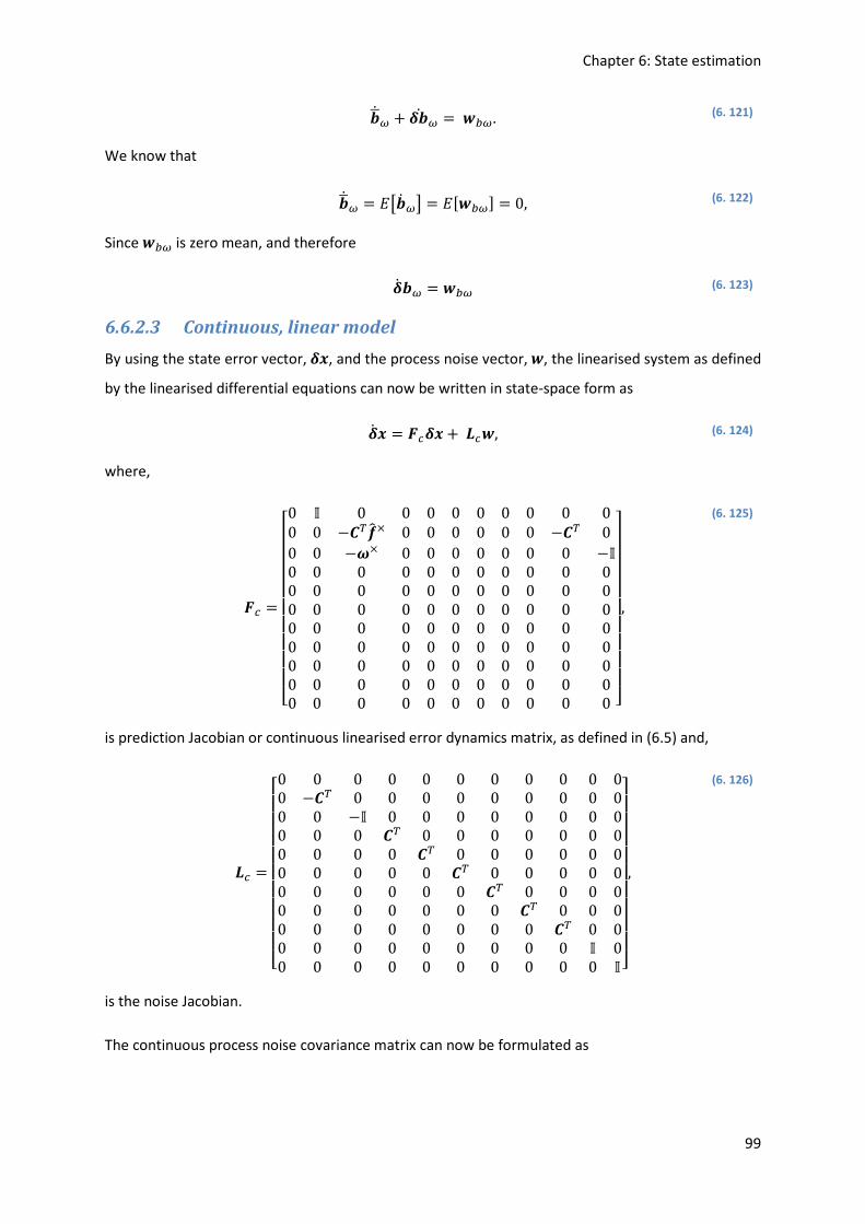
Chapter 6: State estimation
99
��ö� + z�ö � =FJ�. (6. 121)
We know that
��ö� = U)�ö�* = U[FJ�] = 0, (6. 122)
Since FJ� is zero mean, and therefore
zö �� = FJ� (6. 123)
6.6.2.3 Continuous, linear model
By using the state error vector,zP, and the process noise vector,F, the linearised system as defined
by the linearised differential equations can now be written in state-space form as
zö P = VWzP +`WF, (6. 124)
where,
VW =
ÚÛÛÛÛÛÛÛÛÛÜ0 \ 0 0 0 0 0 0 0 0 00 0 −T�q × 0 0 0 0 0 0 −T� 00 0 −h× 0 0 0 0 0 0 0 −\0 0 0 0 0 0 0 0 0 0 00 0 0 0 0 0 0 0 0 0 00 0 0 0 0 0 0 0 0 0 00 0 0 0 0 0 0 0 0 0 00 0 0 0 0 0 0 0 0 0 00 0 0 0 0 0 0 0 0 0 00 0 0 0 0 0 0 0 0 0 00 0 0 0 0 0 0 0 0 0 0 ßà
ààààààààá,
(6. 125)
is prediction Jacobian or continuous linearised error dynamics matrix, as defined in (6.5) and,
`W =
ÚÛÛÛÛÛÛÛÛÛÜ0 0 0 0 0 0 0 0 0 0 00 −T� 0 0 0 0 0 0 0 0 00 0 −\ 0 0 0 0 0 0 0 00 0 0 T� 0 0 0 0 0 0 00 0 0 0 T� 0 0 0 0 0 00 0 0 0 0 T� 0 0 0 0 00 0 0 0 0 0 T� 0 0 0 00 0 0 0 0 0 0 T� 0 0 00 0 0 0 0 0 0 0 T� 0 00 0 0 0 0 0 0 0 0 \ 00 0 0 0 0 0 0 0 0 0 \ßà
ààààààààá,
(6. 126)
is the noise Jacobian.
The continuous process noise covariance matrix can now be formulated as

Chapter 6: State estimation
100
gW = U[FF�] =
ÚÛÛÛÛÛÛÛÛÛÛÜ0 0 0 0 0 0 0 0 0 0 00 g� 0 0 0 0 0 0 0 0 00 0 g� 0 0 0 0 0 0 0 00 0 0 gN,A 0 0 0 0 0 0 00 0 0 0 gN,� 0 0 0 0 0 00 0 0 0 0 gN,K 0 0 0 0 00 0 0 0 0 0 gN,Æ 0 0 0 00 0 0 0 0 0 0 gN,Ý 0 0 00 0 0 0 0 0 0 0 gN,æ 0 00 0 0 0 0 0 0 0 0 gJ� 00 0 0 0 0 0 0 0 0 0 gJ�ßà
àààààààààá
,
(6. 127)
where, U[FF�], is the expected value for FF�.
6.6.2.4 Discrete, linear model
The discrete linear model is derived using a first-order discretisation as presented in [3]. In contrast to
[2], this method simplifies the implementation of the filter and doesn’t affect the filter performance
in any significant way [3]. The discrete linearised error dynamics matrix can be calculated by assuming
a zero-order hold over the time interval ∆< = <?@A − <?, as follows
V? = �V+∆�. (6. 128)
Equation (6.128) can be reduced to first-order to yield
V? ≈ \ + VW∆<. (6. 129)
The discrete linearised error dynamics matrix can now be formulated as
V? =
ÚÛÛÛÛÛÛÛÛÛÜ\ ∆<\ 0 0 0 0 0 0 0 0 00 \ −∆<T_?@�q?× 0 0 0 0 0 0 −∆<T_?@� 00 0 \ − ∆<h× 0 0 0 0 0 0 0 −\∆<0 0 0 \ 0 0 0 0 0 0 00 0 0 0 \ 0 0 0 0 0 00 0 0 0 0 \ 0 0 0 0 00 0 0 0 0 0 \ 0 0 0 00 0 0 0 0 0 0 \ 0 0 00 0 0 0 0 0 0 0 \ 0 00 0 0 0 0 0 0 0 0 \ 00 0 0 0 0 0 0 0 0 0 \ ßà
ààààààààá.
(6. 130)
The discrete process noise covariance matrix can be calculated by assuming a zero-order hold over
the time interval∆< = <?@A − <?, as follows

Chapter 6: State estimation
101
g?QA =¥ �V+(��Q,)`WgW`W��V+-(��Q,)�����Þ �.. (6. 131)
Equation (6.131) can be reduced to first-order to yield
g? ≈ ∆<V?`WgW`W�V?� . (6. 132)
6.6.2.5 Extended Kalman filter prediction equations
The EKF states the prediction equations that follow in this section. The predicted or a priori state
estimate is given by
P7?Q ≔ V?P7?@. (6. 133)
The predicted or a priori state estimate of the covariance matrix is given by
e?@AQ = V?e?@V?� +g? . (6. 134)
6.6.3 Update step
In the update step, the EKF produces the a posteriori estimates by using a measurement to update the
expected value of the state as well as the covariance of the state.
6.6.3.1 Measurement residual
The measurement residual can now be defined as the difference between actual measurements of
the foot positions and their predicted values. The actual measurements are located in the body
coordinate frame, :. Therefore, the predicted values are calculated as the predicted foot positions
minus the predicted centre of body position, transformed from the inertial coordinate frame, $, into
the body coordinate frame,:, with the predicted rotation matrix. The measurement residual can now
be formulated as,
O? ∶=/000019;A,? − T_?Q(57A,?Q −8&?Q)9;�,? − T_?Q(57�,?Q −8&?Q)9;K,? − T_?Q(57K,?Q −8&?Q)9;Æ,? − T_?Q(57Æ,?Q −8&?Q)9;Ý,? − T_?Q(57Ý,?Q −8&?Q)9;æ,? − T_?Q(57æ,?Q −8&?Q)2
33334.
(6. 135)
6.6.3.2 Linearisation of foot position measurement model
For the linearisation of the relative foot position measurement model, (6.48), let
9� ≈ 9'� + z9�, (6. 136)

Chapter 6: State estimation
102
and from (6.58),
T ≈ [\ − z{×]T�. (6. 137)
Substituting (6.136), (6.137), (6.63) and (6.106) into (6.48), yields
9� =9'� + z9� = [\ − z{×]T�[(5� + z5) − (8' + z8)] + 2�. (6. 138)
Expanding (6.138), gives
9'� + z9� = T�(5� − 8') + T�(z5 − z8) − z{×üT�(5� − 8')ý − z{×üT�(z5 − z8)ý + 2�. (6. 139)
From (6.48) we can formulate that
9'1 = T�(5� − 8') + 2�. (6. 140)
Rewriting (6.139) by recognising (6.140), yields
z9� =T�(z5 − z8) − z{×üT�(5� − 8')ý − z{×üT�(z5 − z8)ý. (6. 141)
The term, z{×üT�(z5 − z8)ý, in (6.141) can be neglected due to it being a cross product of state
deviations. The final linearised equation at time step/ can therefore be formulated as
z9�,? = 9�,? − T_?Qü57A,?Q −8&?Qý ≈ −T_?Qz8?Q +T_?Qz5�,?Q + ïT_?Qü5�,?Q −8?Qýð× z{?Q, (6. 142)
corresponding to Bloesch et al.[2].
6.6.3.3 Measurement Jacobian
By substituting the linearised foot position measurement model, (6.142), into the measurement
residual, O?, the measurement Jacobian, as defined in (6.6) can now be derived and formulated as
[? =þO?þP7? (6. 143)
=
ÚÛÛÛÛÛÛÛÛÛÜ−T_0Q � ïT_0Qü5¸,0Q −80Qýð× T_0Q � � � � � � �−T_0Q � ïT_0Qü5¶,0Q −80Qýð× � T_0Q � � � � � �−T_0Q � ïT_0Qü55,0Q −80Qýð× � � T_0Q � � � � �−T_0Q � ïT_0Qü56,0Q −80Qýð× � � � T_0Q � � � �−T_0Q � ïT_0Qü57,0Q −80Qýð× � � � � T_0Q � � �−T_0Q � ïT_0Qü58,0Q −80Qýð× � � � � � T_0Q � �ßà
ààààààààá.

Chapter 6: State estimation
103
6.6.3.4 Measurement noise matrix
The total measurement noise matrix is formed by stacking the all of the single measurement noise
matrices, as defined in (6.47), from . = 1, to . = 6, as a diagonal matrix:
i? =ÚÛÛÛÛÛÛiA,? 0 0 0 0 00 i�,? 0 0 0 00 0 iK,? 0 0 00 0 0 iÆ,? 0 00 0 0 0 iÝ,? 00 0 0 0 0 iæ,?ßàà
àààà.
(6. 144)
6.6.3.5 Extended Kalman filter update equations
The Extended Kalman filter states the update equations that follow in this section. These standard
equations were formulated in the background of this chapter but are given here again, referencing
the specific equations needed to calculate the update step, as derived throughout this chapter.
By using the a priori state estimate covariance matrix as defined in (6.134) together with the
measurement Jacobian, (6.143), and the measurement noise matrix, (6.144), the residual covariance
is calculated as,
l? ≔ [?e?Q[?� + i? . (6. 145)
Combining the a priori state estimate, (6.134), with the measurement Jacobian, (6.143), and the
residual covariance, (6.145), the Kalman gain is calculated as,
^? ≔ e?Q[?�l?QA. (6. 146)
The resulting correction vector is defined as the product of the Kalman gain, (6.146), and the
measurement residual, (6.135), and formulated as,
∆P? ≔ ^?O?, (6. 147)
where the update or a posteriori state estimate is updated using ∆P?:
P7?@ ≔ P7?Q + ∆P? (6. 148)
Note that an extra calculation is needed for the orientation state because the extracted rotational
correction, ∆{?, is of three dimensions, in contrast to the quaternion, that is of four dimensions. The
rotation correction is applied to correct the predicted quaternion, therefore:
67?@ = exp(∆{?)⨂67?Q. (6. 149)
Finally, the update a posteriori estimate of the state covariance matrix is given by

Chapter 6: State estimation
104
e?@ ≔ (\ − ^?[?)e?Q. (6. 150)
6.7 Conclusion
This chapter discussed the state estimation approach used in this study. The state estimation for the
hexapod robot platform was derived using the framework presented by Bloesch et al. [2]. It uses an
EKF to estimate the full state of a robot body by fusing the robot kinematics with an IMU. The chapter
started by providing background information about the EKF. Here, the operation of the EKF was
discussed and the general EKF equations were provided.
Thereafter, the state definition for the EKF was derived. The state vector consists of the position,
velocity and the corresponding quaternion of the centre of the robot body, the contact points of the
six feet with the ground, and the acceleration and angular rate bias values. The corresponding state
error vector was also defined. Next, the prediction model needed by the filter to propagate the state
from one time step to the next, was derived. Here, the set of continuous time differential equations
for the state was derived. By using the kinematic measurement model, derived in Chapter 4, as well
as the joint position measurement model, derived in Chapter 5, the filter measurement model was
derived. The filter measurement model is used in the update step of the EKF.
The chapter concluded by discussing the state estimation’s EKF equations. The filtering convention
was firstly provided followed by the EKF prediction and update steps. For the prediction step, the
continuous time differential equations derived in the filter prediction model, were discretised. Here,
a zero-order hold was assumed with regards to the IMU measurement quantities and the effect of the
incremental rotation was neglected. Next, the continuous time differential equations were linearised
in order to propagate the state estimate covariance matrix through the state dynamics. The linearised
differential equations described the error dynamics. In contrast to [2], the linearised error dynamic
matrix and the discrete process noise covariance matrix were derived using a zero-order hold on the
noise terms as presented by [3]. This simplifies the filter implementation. The prediction step
discussion concluded with the formulation of the a priori state estimate and a priori covariance state
estimate matrix equations.
For the update step, the measurement residual was first formulated as the difference between the
actual foot position measurements and their predicted values. Hereafter, the linearised foot position
measurement model was derived and used to calculate the measurement Jacobian. The measurement
noise matrices, as defined in the filter measurement model, were stacked diagonally to derive the
total measurement noise matrix. Finally, the update equations were discussed. Here, the

Chapter 6: State estimation
105
measurement residual, the measurement Jacobian and the measurement noise matrices together
with the a priori covariance were used to produce the a posteriori estimates. The implementation of
the equations derived in this chapter will be discussed in Chapter 7 together with the state estimation
results.

Chapter 7: Implementation and results
106
Chapter 7: Implementation and results
“An algorithm must be seen to be believed.”
~ Donald Ervin Knuth
7.1 Introduction
This chapter discusses the implementation of the kinematic model and the state estimation as well as
the results of the state estimation. The verification of the kinematic model is firstly discussed.
Thereafter, the state estimation implementation is discussed where, the program architecture is
given, the quantities of the noise parameters for the EKF are derived, and the initialization of the EKF
are discussed. The chapter concludes by presenting and discussing the state estimation results
obtained from multiple experiments.
7.2 Kinematic model and verification
This section discusses the verification of the kinematic model derived in Chapter 4. The kinematic
model equations were implemented in Matlab® as a function that was used by the EKF. In order to
verify the kinematic model results, it had to be compared to reliable reference measurements.
However, measurement information about the robot platform is not supplied by the manufacturers.
Therefore, measurements were taken from the physical platform. CAD models were created of all the
parts of the robot platform and used to build an assembly in SolidWorks®. Fig. 7.1 shows the robot
assembly.
In SolidWorks, specific angles were assigned to the robot joints of the assembly and the foot positions
were then measured. These measurements were taken expressed in the body coordinate frame as
defined in Chapter 4. The same joint angles were used as input for the kinematic model. Multiple tests
were conducted with the robot assembly resembling possible walking poses. The s-axis and t-axis
measurements showed no errors in the millimetre range using the leg kinematic model. A maximum
error of 2mm in the p-axis measurement of the leg kinematic model was found. This error is
distributed in all axes in the robot kinematic model.

Chapter 7: Implementation and results
107
Figure 7. 1: Robot platform assembly model.
The mentioned error in the p-axis of the leg kinematic model is caused by the round foot end. This is
because the length of link 3, representing the tibia of each leg, is defined as the measurement between
joint 3 and the contact point of the foot with the ground. (As defined in Chapter 4.) Therefore,
depending on where the foot end makes contact with the ground, the real length of link 3 changes
and no longer corresponds to the assigned length in the kinematic model. This error is however almost
unnoticeable and included in the kinematic measurement model of the state estimation, verifying the
kinematic model derived.
7.3 State estimation implementation
7.3.1 Program architecture
This section discusses the implementation of the state estimation as derived in Chapter 6. The EKF
equations were implemented in Matlab®. Fig. 7.2 shows the architecture diagram for the main part
of the code. In Fig 7.2, each function is enclosed in a different coloured block. Corresponding coloured
arrows indicate how the output of a specific function is used as input in another function. The Matlab®
code with a detailed discussion about all the functions used to implement the state estimation, can
be found in Appendix A.
The code begins by extracting all of the measured data that were captured by the platform into
Matlab®. The sensor data acquisition was discussed in detail in Chapter 5. Hereafter, the initialisation

Chapter 7: Implementation and results
108
needed by the EKF is performed. This consists of declaring all the noise parameters, an initial state
vector and an initial covariance matrix. The quantities assigned to the noise parameters are derived
and discussed in section 7.3.2. The initial state vector and covariance matrix is needed to start the EKF
loop. The derivation of the initial state vector and the initial covariance matrix are discussed in section
7.3.3.
Figure 7. 2: State estimation program architecture diagram.

Chapter 7: Implementation and results
109
After the initialisation, the EKF loop is entered for data point one, (time step one), until the end of the
data is reached. The end of the data is identified as the number of points (NOP) captured by the data
acquisition process. The EKF loop starts with the prediction step. First the IMU bias values are
corrected as derived in (6.62) and (6.65).
Next the a posteriori quaternion estimate is converted to a rotation matrix with the function
“Quadernion_to_RotationMatrix” that implements (6.15). The dynamic model matrix is then
calculated with the function “dynamic_model_matrix” that implements (6.130). Using the dynamic
model matrix and the a posteriori rotation matrix, the function “noise_covariance_matrix” calculates
the noise covariance matrix as defined in (6.132). The dynamic model matrix is then used to update
the a priori state estimate as defined in (6.133). The noise covariance matrix together with the
dynamic model matrix is used to update the a priori covariance matrix as defined in (6.134). This
concludes the prediction step.
In the update step, the a priori quaternion estimate is firstly converted to a rotation matrix with the
“Quadernion_to_RotationMatrix” function. Thereafter, the measurement residual is calculated using
the measured foot positions and the a priori estimated foot positions with the function
“y_measurement_residual” implementing (6.135). The measured foot positions are calculated with
the “Kinematic_model” function implementing the kinematic model derived in Chapter 4. The
measurement Jacobian is then calculated with the “H_measurement_Jacobian” function
implementing (6.143). The total measurement noise matrix is computed using the defined noise
parameters with the function “R_measurement_noise” implementing (6.47) and (6.144). The update
step is completed with the calculation of the a posteriori state estimate and covariance using (6.145)-
(6.150). The EKF loop is then repeated for all the data points.
When using (6.149) a drift was noticed in the estimation that resulted in inaccurate position
estimation. A modified method was used to convert the rotational correction vector to a quaternion
correction [83]. Here, the rotation vector was interpreted as Euler angles,D9 = [( } :]�, where, (, represents the pitch, }, represents the roll and, :, represents the yaw. The following equation was
used to calculate the quaternion correction:

Chapter 7: Implementation and results
110
6 =ÚÛÛÛÛÛÛÛÜ cos�
(2� cos �:2� sin �}2� − sin �(2� cos �}2� sin �:2�cos�(2� sin �}2� sin �:2� − cos �}2� cos �:2� Å.¿ �(2�cos�(2� cos �}2� sin �:2� + sin �(2� cos �:2� sin �}2�cos�(2� cos�}2� cos�:2� + sin �(2� sin �}2� sin �:2� ßàààààààá.
(7. 1)
This quaternion correction value was then used to correct the predicted quaternion.
7.3.2 Noise parameters
This section discusses the values assigned to the noise processes in the EKF. Initial standard deviations
for the noise parameters were derived first. Thereafter, the noise parameters were empirically tuned
to a point where the EKF presented the best state estimation results.
The discrete standard deviations of the additive white Gaussian noise processes, F� and F�, affecting
the IMU measurement quantities, were obtained by dividing the root PSD values (provided in Chapter
5) by the root of the sampling time [87],
�Fø� = 0.00078√∆< m/s�, (7. 2)
�Fú� = 0.000523√∆< rad/s. (7. 3)
The initial variance quantities for covariance matrices, g� and g�, where then obtained by squaring
the standard deviations as defined in (7.2) and (7.3). For ∆< = 0.05s, these variance quantities are
given as
�Fø�� = 1.231 × 10QÝ, (7. 4)
�Fú�� = 5.483 × 10Qæ. (7. 5)
For covariance parameters, gJ� and gJ�, the initial discrete standard deviations of the white
Gaussian noise processes, FJ� and FJ�, were derived by multiplying the continuous-time standard
deviations defined in Chapter 5 by the square of the sampling time [87],
�Fùø; = 0.0001√∆<m/s�, (7. 6)

Chapter 7: Implementation and results
111
�Fùú� = 0.000618√∆<rad/s. (7. 7)
The initial variance quantities for covariance matrices, gJ� and gJ�, were then obtained by squaring
the standard deviations as defined in (7.6) and (7.7). For ∆< = 0.05s, these variance quantities are
given as
�Fø;� = 5 × 10QAÇ, (7. 8)
�Fú�� = 1.9097 × 10Q<. (7. 9)
For covariance matrix, i4, the initial standard deviation of the discrete Gaussian noise process, 24,
representing the error in the joint position feedback were defined as given in Chapter 5:
�2õ = 0.0087rad. (7. 10)
From (7.9) the initial variance quantity as used in the EKF were calculated as
�2õ� = 0.0087�. (7. 11)
For the kinematic measurement model, as defined in Chapter 4, the additive discrete Gaussian noise
term, 23,�, representing the error in the kinematic model, can be defined using the kinematic model
validation test results. Let the maximum error in any axis direction of the kinematic model be defined
as the standard deviation of 23,�, �2=,> = 0.002m. (7. 12)
The variance quantity used as the initial value of the covariance parameter, i3,�, was then calculated
as
�2=,>� = 0.000004. (7. 13)
For the covariance parameter, gN,�, as defined in Chapter 6, the standard deviation of the white noise
process, FN,�, allowing a certain amount of foot slippage, were defined as
�F?,> =7.071 × 10QÝ√∆< m, (7. 14)

Chapter 7: Implementation and results
112
so that for ∆< = 0.05s, the initial variance is calculated as
�F?,>� = 1 × 10Q@. (7. 15)
In order to compensate for inaccuracies and assumptions in the filter model, the initial noise
parameters were empirically tuned until the state estimation showed the best results. Table 7.1
summarises the final standard deviation noise parameter values used in the EKF.
Table 7. 1: Final standard deviation values of the noise parameters.
Noise parameter Standard deviation (discrete) 24 �2õ = 0.2rad 23,� �2=,> = 0.002m F� �Fø = 0.234√∆< m/s�
F� �Fú = 0.157√∆< rad/s FJ� �Fùø = 0.03√∆<m/s� FJ� �Fùú = 0.184√∆<rad/s FN,� �F?,> =7.071 × 10QÝ√∆< m
The variances of the noise parameters were obtained by squaring the standard deviation values as
given in Table 7.1. The standard deviations of the noise parameters 23,� and FN,�, remained the same
as initially assigned. The standard deviation of the joint position noise parameter,24, and all the IMU
noise parameters, F� , F�, FJ� and FJ�, increased.
The joint position measurement feedback were scaled from a 10 bit feedback value to an 8 bit
feedback value. This decreased the joint position feedback accuracy and can account for the increased
noise parameter value. Since the IMU used in this study is a low-cost MEMS device, the increase of
the IMU noise parameters were expected. Another notable source that can account for the increased
IMU noise parameters is the vibration of the robot. Vibration directly influences the accuracy of
inertial devices, therefore the use of low-cost IMUs on devices prone to vibration is not recommended.

Chapter 7: Implementation and results
113
7.3.3 Initialisation
This section discusses the initial values assigned to the state vector and covariance matrix. These initial
values are needed to start the EKF loop and can influence the settling time of the filter. Since any
navigation period of the robot will start with the robot motionless, sensor data was recorded for a
period of time with the robot at stand still. This data was then used to run the EKF with random initial
values. The results of this test showed that the filter settled at specific values for the a posteriori state
estimation. These settled values were assigned as the initial values for the robot’s state.
For the position of the centre of the body expressed in the inertial coordinate frame, 8 = [1,1,1.9]�.
For the velocity of the centre of the body expressed in the inertial coordinate frame, E = [0,0,0]�.
For the quaternion representing the orientation of the centre of the body expressed in the inertial
coordinate frame, 6 = [0,0,0,1]�. Expressed in the body coordinate frame, the acceleration bias, �� = [0,0,0]�, and the angular rate bias, �� = [0,0,0]�. Even though the robot will begin its
navigation motionless, the robot’s foot positions can differ. Therefore, the first foot positions as
calculated by the kinematic model was used. The kinematic model output is however expressed in the
body coordinate frame. In order to express the foot positions in the inertial coordinate frame, the
initial centre of body position values were added to the kinematic model results to produce the initial
foot position values, 5� = 9� + 8. For simplicity, the initial covariance matrix were defined as, e =0.0001 × [\]KK×KK.
7.4 State estimation results
7.4.1 Test description
A series of experiments were performed using the hexapod platform. During these experiments, the
sensor data for the state estimation were collected as discussed in Chapter 5, and ground truth
measurements were independently collected by a Vicon motion capture system. The collected sensor
data were used as input for the EKF code implemented in Matlab® to provide the estimation. For all
of the experiments conducted, the comparison between the estimation and the ground truth
measurements was investigated to validate the state estimation approach implemented in this study.
Background on the Vicon system and the use of it as well as the current control of the robot will now
be discussed.

Chapter 7: Implementation and results
114
7.4.1.1 Vicon system
The Vicon system is a motion capturing system that tracks rigid bodies in 3D space [4]. The specific
system used in this study consists of twelve cameras. Through a software interface and two I/O
machines, these cameras tracked reflective markers that were placed on the robot platform. Fig 7.3
shows the robot platform used in this study with the markers placed on it.
Figure 7. 3: Robot platform with Vicon markers.
Upon start-up of the system, all noise in the Vicon’s arena was first filtered out. The system was further
calibrated with an accurately calibrated object known as a wand. The Vicon calibration concluded with
the setting of an origin using the wand. Next, the robot platform, with the reflective markers on it,
was placed in the Vicon arena. In order to create an object representing the platform, specific markers
were selected and a reference frame location was defined. The reference frame location was set to
correspond to the body coordinate frame as defined in the state estimation. The platform’s motion
was then tracked and recorded through the created object for all of the conducted experiments. Fig.
7.4 shows the Vicon software environment with the created object.

Chapter 7: Implementation and results
115
Figure 7. 4: Vicon software environment.
For each time step, <, two vectors describing the reference frame were recorded by the Vicon system.
The first was a position vector, 8E = [ , Ù, M], describing the , Ù and M positions of the origin of the
reference frame. The second was a quaternion, 6E = [�Ç, �A, ��, �K], describing the orientation of the
reference frame.
The velocity of the reference frame origin was calculated as the numerical position derivative,
EA = ∆8E∆B . (7. 16)
The Euler angle vector, defined as
D = [( } :]� , (7. 17)
where, the symbol, (, represents the pitch, the symbol, }, represents the roll and the symbol, :,
represents the yaw, were calculated using 6E as follows [83]:
D = ´�<�¿2(−2�A�K + 2�Ç��,�K� − ��� − �A� + �Ç�)�Å.¿(2���K + 2�Ç�A)�<�¿2(−2�A�� + 2�Ç�K,��� − �K� + �Ç� − �A�)µ. (7. 18)
7.4.1.2 Robot control
The control of the robot is out of the scope of this study. In order to test the state estimation computed
for the robot platform, open source code was uploaded onto the platform’s ArbotiX-M Robocontroller
which allowed the platform to be controlled by an ArbotiX commander. Both these devices were

Chapter 7: Implementation and results
116
included in the PhantomX Mark II kit from Trossen Robotics [51]. The open source code used as
firmware for the platform is known as the “PhantomX Hexapod Phoenix Code” and is distributed
through Trossen Robotics [88]. The current control approach is limited to relatively even terrain. The
firmware was modified to send out the servo positions which increased vibrations on the robot when
navigating. The firmware offers a variety of control options including different gait possibilities, body
movement and speed control which were used in the experiments conducted.
7.4.2 Results and discussion
This section provides the results obtained from multiple experiments conducted with the robot
platform. Due to the limited control of approach of the robot, all the experiments were conducted on
relatively even terrain. The experiments were conducted in such a manner to validate the state
estimation approach by focussing on the accuracy of the estimates for the full body pose needed for
control of a robot.
In order to validate that the state estimation does not depend on a specific gait, two experiments
implementing two different gaits were conducted. In both experiments the robot navigated on even
terrain in a square form. Since the yaw angle is not fully observable, the experiments were conducted
without the robot turning. In the first experiment the robot navigated using a ripple gait while in the
second, the robot navigated with a tripod gait. Fig. 7.5 and Fig. 7.6 shows the comparison between
the estimated position and the Vicon system’s position outputs of the robot with a ripple and a tripod
gait respectively.
Figure 7. 5: Comparison of the estimated position and the Vicon position outputs for ripple gait.

Chapter 7: Implementation and results
117
Figure 7. 6: Comparison of the estimated position and the Vicon position outputs for tripod gait.
A small drift in the position estimates occurs in the results of both the experiments. This is due to the
position not being fully observable. The ripple gait estimation shows a drift of 5 % in the p-axis position
and 1 % in the s-axis position of the travelled distance. The tripod gait estimation’s drift amounts up
to 9 % in the p-axis position and 8 % in the s-axis position of the travelled distance. Increased
vibrations on the robot when navigating with tripod gait compared to ripple gait caused the drift
difference between the two experiments. The vibrations increase errors in the IMU data, especially in
the t-axis of the body coordinate frame, and is caused by the current control approach. The influence
of the vibration of the robot on the estimation can also be noticed in the t-axis position estimation of
the experiments. Fig. 7.7 shows the comparison between the M position estimation of the tripod and
ripple experiments.
Figure 7. 7: Comparison between the z position estimation of the ripple and tripod experiment.
Bloesch et al. [2] observed a 10 % drift in their estimation results and stated that notable sources of
the drift include inaccurate leg kinematics and fault-prone contact detection. Even though the
experiments done in this study are not exactly the same as that done by Bloesch et al. [2], it can be
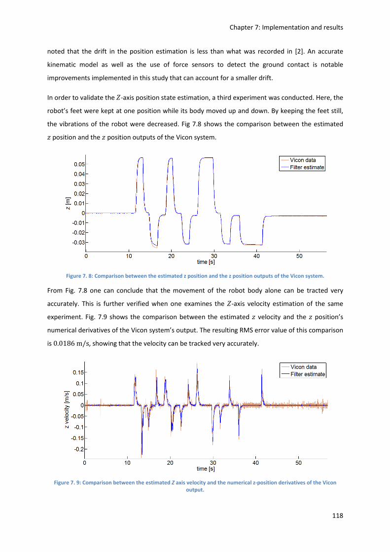
Chapter 7: Implementation and results
118
noted that the drift in the position estimation is less than what was recorded in [2]. An accurate
kinematic model as well as the use of force sensors to detect the ground contact is notable
improvements implemented in this study that can account for a smaller drift.
In order to validate the t-axis position state estimation, a third experiment was conducted. Here, the
robot’s feet were kept at one position while its body moved up and down. By keeping the feet still,
the vibrations of the robot were decreased. Fig 7.8 shows the comparison between the estimated Mposition and the M position outputs of the Vicon system.
Figure 7. 8: Comparison between the estimated z position and the z position outputs of the Vicon system.
From Fig. 7.8 one can conclude that the movement of the robot body alone can be tracted very
accurately. This is further verified when one examines the t-axis velocity estimation of the same
experiment. Fig. 7.9 shows the comparison between the estimated M velocity and the M position’s
numerical derivatives of the Vicon system’s output. The resulting RMS error value of this comparison
is 0.0186m/s, showing that the velocity can be tracked very accurately.
Figure 7. 9: Comparison between the estimated Z axis velocity and the numerical z-position derivatives of the Vicon
output.

Chapter 7: Implementation and results
119
Next, an experiment was conducted to investigate the yaw, pitch and roll estimations when only the
body is moving. Here, the robot body performed a set of clockwise and anti-clockwise turns followed
by a set of forward and backward tilting and ended with a set of sideways tilting. Fig. 7.10 shows the
comparison between the estimated yaw, pitch and roll angles and the Vicon system’s orientation
outputs. This experiment validated very precise estimation for the robot body moving with the angular
RMS error 0.0138rad for the yaw, 0.0069rad for the pitch, and 0.0119rad for the roll.
Figure 7. 10: Comparison between the estimated yaw, pitch and roll angles and the orientation outputs of the Vicon
system.
Since the yaw isn’t fully observable, a drift in the yaw estimation is expected while the robot is
navigating. The following two experiments were conducted to investigate any possible drift in the yaw
estimation. In both experiments the robot navigated on even terrain producing multiple turns using
ripple gait. In the first experiment the angles of the turns were small (less than 90°). Fig. 7.11 shows
the comparison between the estimated yaw and the Vicon system’s yaw output for this experiment.
The comparison between the estimated position and the Vicon system’s position outputs is also
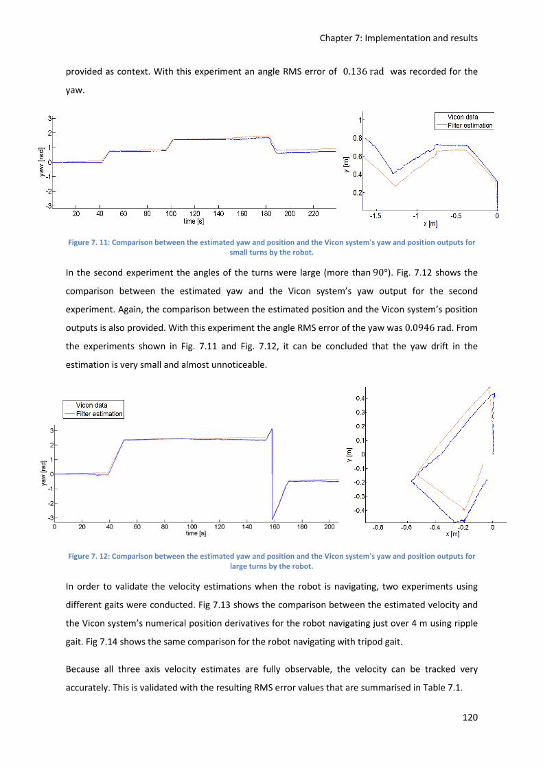
Chapter 7: Implementation and results
120
provided as context. With this experiment an angle RMS error of 0.136rad was recorded for the
yaw.
Figure 7. 11: Comparison between the estimated yaw and position and the Vicon system's yaw and position outputs for
small turns by the robot.
In the second experiment the angles of the turns were large (more than90°). Fig. 7.12 shows the
comparison between the estimated yaw and the Vicon system’s yaw output for the second
experiment. Again, the comparison between the estimated position and the Vicon system’s position
outputs is also provided. With this experiment the angle RMS error of the yaw was0.0946rad. From
the experiments shown in Fig. 7.11 and Fig. 7.12, it can be concluded that the yaw drift in the
estimation is very small and almost unnoticeable.
Figure 7. 12: Comparison between the estimated yaw and position and the Vicon system's yaw and position outputs for
large turns by the robot.
In order to validate the velocity estimations when the robot is navigating, two experiments using
different gaits were conducted. Fig 7.13 shows the comparison between the estimated velocity and
the Vicon system’s numerical position derivatives for the robot navigating just over 4 m using ripple
gait. Fig 7.14 shows the same comparison for the robot navigating with tripod gait.
Because all three axis velocity estimates are fully observable, the velocity can be tracked very
accurately. This is validated with the resulting RMS error values that are summarised in Table 7.1.

Chapter 7: Implementation and results
121
Table 7. 2: RMS error values for ripple and tripod gait velocities.
RMS error [m/s]
Axis velocity [m/s] Ripple gait experiment Tripod gait experiment
x 0.034 0.079
y 0.0427 0.0689
z 0.0258 0.0452
A notable source for the higher RMS error values for the tripod gait compared to the ripple gait is
again due to the increased vibrations of the robot when navigating using tripod gait. The RMS error
values recorded in these experiments are comparable to the results published in [2].
Figure 7. 13: Comparison between the estimated velocity and the Vicon system’s numerical position derivatives for the
robot navigating using ripple gait.

Chapter 7: Implementation and results
122
Figure 7. 14: Comparison between the estimated velocity and the Vicon system’s numerical position derivatives for the
robot navigating using tripod gait.
For the experiment shown in Fig. 7.13, where the robot is navigating in ripple gait, the comparison
between the position estimates and the Vicon system’s position outputs are provided in Fig. 7.15. Fig.
7.15 includes the foot position estimates for leg one, four and five, as defined by Fig. 4.8. This figure
shows how the robot actions can accurately be tracked by following the foot position estimates. The
robot’s starting position is with its centre of body position at 8 = [0,0,0]. From the positions of the
feet, one can determine that the robot is facing forward in the positive Ù direction.
The robot’s movements can now be derived from Fig 7.15 as follows:
• The robot walked forward for ±0.4 m,
• then turned just over 90° anti-clockwise,
• walked forward for ±1.5 m,
• turned just under 90° anti-clockwise,
• walked forward for ±1 m,
• waked sideways (left) for ±1.5 m,
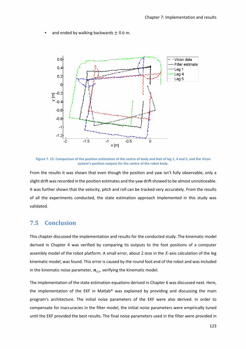
Chapter 7: Implementation and results
123
• and ended by walking backwards ±0.6 m.
Figure 7. 15: Comparison of the position estimation of the centre of body and feet of leg 1, 4 and 5, and the Vicon
system’s position outputs for the centre of the robot body.
From the results it was shown that even though the position and yaw isn’t fully observable, only a
slight drift was recorded in the position estimates and the yaw drift showed to be almost unnoticeable.
It was further shown that the velocity, pitch and roll can be tracked very accurately. From the results
of all the experiments conducted, the state estimation approach implemented in this study was
validated.
7.5 Conclusion
This chapter discussed the implementation and results for the conducted study. The kinematic model
derived in Chapter 4 was verified by comparing its outputs to the foot positions of a computer
assembly model of the robot platform. A small error, about 2mm in the p-axis calculation of the leg
kinematic model, was found. This error is caused by the round foot end of the robot and was included
in the kinematic noise parameter, 23,�, verifying the kinematic model.
The implementation of the state estimation equations derived in Chapter 6 was discussed next. Here,
the implementation of the EKF in Matlab® was explained by providing and discussing the main
program’s architecture. The initial noise parameters of the EKF were also derived. In order to
compensate for inaccuracies in the filter model, the initial noise parameters were empirically tuned
until the EKF provided the best results. The final noise parameters used in the filter were provided in
Chapter 7: Implementation and results
124
Table 7.1. The discussion on the implementation of the state estimation concluded with the derivation
of the initial state vector and covariance matrix needed by the EKF.
Lastly, the state estimation results were discussed. Numerous experiments were conducted where
the state estimation outputs of the robot platform were compared to a ground truth measurements
taken by a Vicon system. As the control of the robot is out of the scope of this study, these experiments
were conducted with a limited control approach on relatively even terrain. Even though it was verified
that the state estimation does not depend on specific locomotion gaits, increased vibrations of the
robot for certain gaits caused by the robot control, influenced the estimation results. As result, the
drift in the position estimation for ripple gait was less than for tripod gait. For both locomotion gaits,
the position drift noticed was under 9%, less than what was recorded in [2].
With an experiment where the robot body was tilted and turned, the estimation of the yaw pitch and
roll was validated. Here, angular RMS errors of less than 0.01rad was recorded. Since the yaw isn’t
fully observable, further experiments were conducted where the yaw drift was investigated for the
robot navigating with smaller and larger turns. It was concluded that the yaw drift is very small and
almost unnoticeable. The velocity estimation were evaluated with two experiments where the robot
was navigating randomly using ripple and tripod gaits. For the ripple gait, RMS errors of less than 0.04m/s were recorded. For the tripod gait, RMS errors of less than 0.08m/s were recorded. These
experiments showed that the velocity can be accurately tracked. The state estimation results
concluded by showing how the robot’s actions can be tracked by considering the estimation of the
foot positions together with the estimation of the centre of the robot body.
All of the experiments conducted showed comparable results to those found by Bloesch et al.[2]. With
the validation of the state estimation for the hexapod robot using only proprioceptive sensors, this
study concludes.
Chapter 8: Conclusion and future work
125
Chapter 8: Conclusion and future work
“Imagination is more important than knowledge.
Knowledge is limited. Imagination encircles the world.”
~ Albert Einstein
8.1 Summary of work done
This study started with a need identified for the development of a robot that can operate in almost
any land-based environment. In Chapter 2 research focussed and directed this need to the problem
statement of this study: the development of a state estimation approach for a hexapod platform using
only proprioceptive sensors. Through a literature study presented in Chapter 3, a commercial hexapod
robot and common proprioceptive sensors were acquired. A framework for the state estimation of
the hexapod platform was also identified. The framework was based on the fusion of the robot’s
kinematics with inertial sensor data. Hereafter, the sensory devices were integrated onto the hexapod
robot to develop the robot platform used to validate this study.
It was identified that the state estimation framework will require a kinematic model of the robot
platform. Therefore, in Chapter 4 a kinematic model for the robot platform was derived. This was done
using the Denavit-Hartenberg notation. As no measurement details about the hexapod robot is
provided by the manufacturers, this derivation is seen as a contribution made by this study. A
measurement model for the kinematic model, needed by the state estimation, was also derived.
In Chapter 5 all of the sensory devices needed for the state estimation were discussed. The data
acquisition method was also discussed and implemented. To account for errors in the sensor
measurements, measurement models were derived that were used in the state estimation equations.
The state estimation framework presented by Bloesch et al. [2] was then adopted for the hexapod
platform. The state estimation methodology and the derivation of the state estimation equations were
discussed in Chapter 6. All of the state estimation equations were derived for the hexapod platform
in order to provide six degrees of freedom information about the robot base. In addition, the foot
positions of the robot were also estimated and force sensors in the robot’s feet were used to provide
ground contact status.
The state estimation equations were then implemented in Matlab® for evaluation. This was discussed
in Chapter 7. Initial noise parameters were derived for the EKF. With the robot recording sensor data,

Chapter 8: Conclusion and future work
126
a few simple experiments were used to derive an initial state vector and covariance matrix needed by
the EKF. These experiments were also used to empirically tune the noise parameters until the EKF
provided the most accurate state estimation. Final experiments were then conducted to compare the
state estimation results with ground truth measurements. The state estimation approach was then
validated.
8.2 Evaluation of state estimation approach
In this study a state estimation framework was successfully used to develop a state estimation
methodology and derive state estimation equations for a hexapod platform. The state estimation
methodology implemented uses an EKF to fuse the robot kinematics with IMU measurements. The
filter can handle any gait as well as unstructured terrain with the assumption of limited foot slippage.
It estimates the position, velocity and orientation at the robot’s centre. This results in a full six degrees
of freedom pose estimation of the robot base. As mentioned in Chapter 2, a six degrees of freedom
pose estimation is especially important for the stability control of legged robots navigating in
unstructured terrain.
Furthermore, the positions of the feet of the robot and the bias quantities of the IMU is also estimated.
The state estimation approach can also be interpreted as a simultaneous localisation and mapping
algorithm, where the estimated foot contact positions can be used to build a map. The use of only
proprioceptive sensors as input to the state estimator is important. This will allow the robot to be
controlled without having to rely on exteroceptive sensors such as a GPS or camera.
The state estimation approach was verified and validated in Chapter 7. Even though the absolute
position is not fully observable, a drift in the position estimate of less than 5% of the distance
travelled was recorded when ripple gait was used for the robot’s locomotion. This drift percentage is
lower than recorded by Bloesh et al. [2]. The inclusion of the force sensors for ground detection and
an accurate kinematic model are notable sources for this improvement. The estimation of the velocity
of the robot base was very precise yielding RMS error values of less than 0.04m/s for the robot using
ripple gait. The roll and pitch estimations was also very precise and the expected yaw drift showed to
be almost unnoticeable. These results are all comparable to those found by Bloesch et al. [2]
When evaluating the state estimation approach, one can conclude that it can easily be implemented
on low-cost commercially available hexapod robots using common low-cost sensory devices. Its
accuracy is ideal for further research and the development of control algorithms and robotic
applications.
Chapter 8: Conclusion and future work
127
8.3 Improvements and future work
In order to improve the current state estimation methodology the inclusion of measurements of the
forces acting on the legs of the robot can be considered. By adding leg force estimations, the operating
safety of the servo motors can be monitored. This can provide vital information, especially when the
robot is navigating autonomously in an unstructured environment.
In the paper “Neural virtual sensors for terrain adaptation of walking machines.” presented by
Estremera et al. [62] a virtual force sensor is presented. The virtual force sensor uses sensory
information from joint position feedback to eliminate the need for physical force sensors in the robots
feet. The research done by Estremera et al. [62] let to the following hypothesis with regards to
improvements and future work.
By comparing the full body estimate with the force information from the force sensors, a virtual sensor
can be developed that will estimate the forces in the body and the ground contact of the feet. After a
virtual force sensor is designed and trained the physical force sensors in the feet of the hexapod can
be eliminated from the robot design. This will result in a state estimation that makes use of more
sensory information than the one presented by Bloesch et al. [2] but has the same amount of physical
sensors.
Future work can also include handling the absolute position and yaw estimations that isn’t fully
observable. Apart from the triaxial accelerometer and the triaxial gyroscope, the IMU used in this
study also has a triaxial magnetometer. By including the magnetometer measurements in the state
estimation algorithms, one can expect a reduction in the yaw drift noticed in the current estimation
approach.
It is important to note that the state estimation for a legged robot should only rely on proprioceptive
sensors for stability control. However, by including measurements from a GPS, the absolute position
can be estimated. The estimation will therefore still only rely on the proprioceptive sensors but an
additional exteroceptive sensor can be used to correct the robots absolute position whenever needed.
Possible future work with regard to the robot platform include the development of a control approach
that uses the state estimation as derived in this study. This will allow further testing of the state
estimation approach as well as development toward an end application. Since the platform is classified
as low-cost, it can easily be replaced. Therefore, the platform can be sent into dangerous situations.
End applications of the robotic platform is mainly focussed on search and rescue missions.

Chapter 8: Conclusion and future work
128
8.4 Conclusion
The objective of this study was to develop and implement a state estimation approach for a hexapod
robot that only relies on proprioceptive sensors. The approach had to be easily implemented on a low-
cost commercially available hexapod robot with common low-cost sensors. From the results it is
shown that such an approach was developed and successfully implemented.
The state estimation approach was validated and can now be used to develop and test control
algorithms for hexapod robots.

APPENDIX
129
APPENDIX
Appendix A: Code
Matlab code
In order to verify and validate the state estimation methodology derived in this study, the state
estimation equations were implemented in Matlab®. All of the Matlab® code is available on the
dissertation cd in the “Matlab code” folder. The code is commented in detail with the function names
corresponding to the discussion in Chapter 7.
Arduino code
This section discusses the open-source “PhantomX Hexapod Phoenix Code” firmware and the
modifications that were made to the firmware code for the control of the robot platform used in this
study. The open-source firmware along with detailed documentation on how to implement it can be
found at [88].
Compared to the original firmware supplied by the distributers of the PhantomX hexapod, the Phoenix
code provide life-like walking gaits and much more features. Some of the features used in this study
include: translate mode, rotate mode, speed control, t- axis control and a variety of different gait
options. The specific firmware version used in this study can be found in the “Arduino code” folder
included in the dissertation cd.
Two modifications were implemented in the firmware code. The first addressed the servo motor’s
position feedback needed for the state estimation developed in this study. Here, a timer was
implemented in order to send out the servo positions every 50ms. This was done by reading the
present position value in the “AX_PRESENT_POSITION_L” register of each Dynamixel servo motor’s
microcontroller into an array. The second modification involved the implementation of a software
serial library in order to communicate the position feedback array to the UDOO single board computer
used to capture all the sensor data.
In the “Arduino code” folder, the executable program named “PhantomX_V2_Commander-
_AX12_Stock_Rev_a” was loaded as firmware onto the robot platform for this study. In
“Phoenix_Code.h” the “SoftwareSerial.h” and the “SimpleTimer.h” files were included and a software

APPENDIX
130
serial named “mySerial”, was opened at 115200 baud rate. In “Phoenix_Driver_AX12.h” the
“SoftwareSerial.h” and the “SimpleTimer.h” files were included again and the RX and TX hardware
pins for “mySerial” was assigned. These pins were physically connected to input pins on the UDOO to
create the serial communication line. A timer named “timer” was also declared and a function named
“BeenPos” was included. This function reads all 18 servo positions into an array and sends it out on
the software serial line. The “BeenPos” function is called every 50ms by the timer.
Python code
This section expands on the discussion provided in Chapter 5 about the executable program used to
acquire and collect the sensory data from the sensory devices. The program was implemented in
Python IDE on the UDOO single board computer that was integrated onto the robot platform. The
complete program code is included on the dissertation cd in the folder “Python code”.
The program starts by entering a WHILE loop that monitors if the sensor data collection should start.
The start and stop condition for the program is controlled by a hardware button that is connected to
a general in-out pin (gpio) with identification number 123, of the UDOO. Whenever the push button
is triggered, the register value of the pin it is connected to change from 0 to 1. In the WHILE loop the
register of this pin is constantly opened and read until its value is 1. The following lines of code
implements the opening and reading of the register:
button_read = open("/sys/class/gpio/gpio123/value",'r')
val = button_read.read(1)
Here, “/sys/class/gpio/gpio123/value" is the directory to the pin-123, and 'r' opens this directory in
read mode. When “val” is equal to 1, the following is implemented in an IF condition: Firstly, an LED
connected to gpio56 is turned on for visual conformation to the person operating the platform. This
is implemented by opening the directory of gpio56 in write mode, ‘w’, and writing the value 1 in it:
led_on = open("/sys/class/gpio/gpio56/value",'w')
led_on.write('1')
For conformation in the operating system on the UDOO, the program also writes “BEGIN” to the
Python IDE:
print("BEGIN")
Hereafter, the setup of serial communication with the IMU is implemented. The 3DM-GX3-25 device
was connected to one of the USB ports on the UDOO. In the WHILE loop the communication with the
USB port is established by calling the function “open_Inertial()”. This function uses a serial library to

APPENDIX
131
communicate with the 3DM-GX3-25 device. The communication protocol of the 3DM-GX3-25 can be
found on the MicroStrain website [80]. The serial communication between the UDOO and the IMU
was established with the following code:
def open_Inertial():
global inertial
inertial = serial.Serial(
port='/dev/ttyACM0',
baudrate=115200,
parity=serial.PARITY_NONE,
stopbits=serial.STOPBITS_ONE,
bytesize=serial.EIGHTBITS,
timeout=1
)
inertial.close()
inertial.open()
return inertial
Next, the serial communication needed in order to read the servo positions send through a software
serial communication protocol from the ArbotiX board to the UDOO was established. The output from
the ArbotiX board was connected to the “ttymxc3” port on the UDOO. The following code was used
to establish communication with this port:
def open_Serial():
global ser
ser = serial.Serial(port='/dev/ttymxc3',
baudrate=115200,
parity=serial.PARITY_NONE,
stopbits=serial.STOPBITS_ONE,
bytesize=serial.EIGHTBITS,
timeout=1
)
ser.close()
ser.open()
return ser
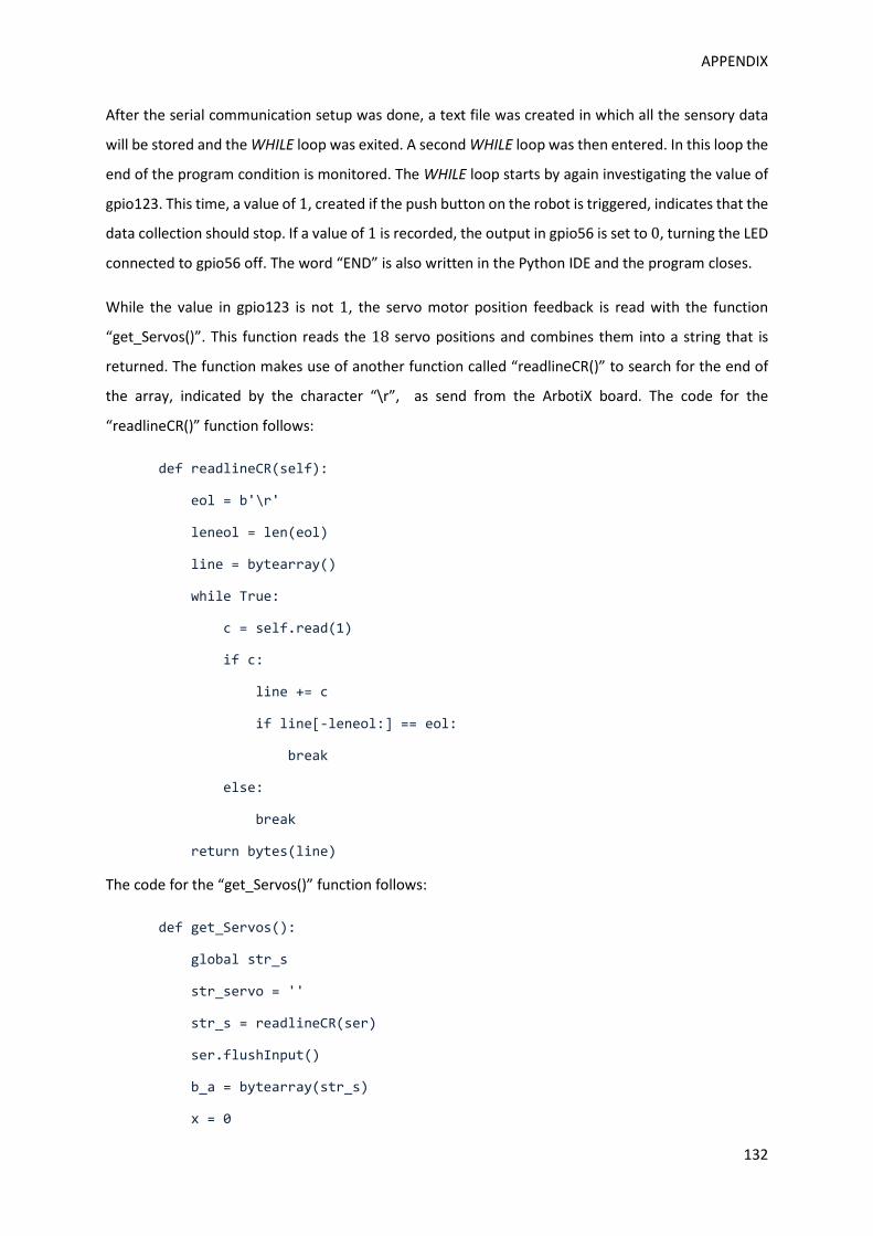
APPENDIX
132
After the serial communication setup was done, a text file was created in which all the sensory data
will be stored and the WHILE loop was exited. A second WHILE loop was then entered. In this loop the
end of the program condition is monitored. The WHILE loop starts by again investigating the value of
gpio123. This time, a value of 1, created if the push button on the robot is triggered, indicates that the
data collection should stop. If a value of 1 is recorded, the output in gpio56 is set to 0, turning the LED
connected to gpio56 off. The word “END” is also written in the Python IDE and the program closes.
While the value in gpio123 is not 1, the servo motor position feedback is read with the function
“get_Servos()”. This function reads the 18 servo positions and combines them into a string that is
returned. The function makes use of another function called “readlineCR()” to search for the end of
the array, indicated by the character “\r”, as send from the ArbotiX board. The code for the
“readlineCR()” function follows:
def readlineCR(self):
eol = b'\r'
leneol = len(eol)
line = bytearray()
while True:
c = self.read(1)
if c:
line += c
if line[-leneol:] == eol:
break
else:
break
return bytes(line)
The code for the “get_Servos()” function follows:
def get_Servos():
global str_s
str_servo = ''
str_s = readlineCR(ser)
ser.flushInput()
b_a = bytearray(str_s)
x = 0

APPENDIX
133
while x < 18 :
str_servo = str_servo + str(b_a[x]) + ','
x = x + 1
a_bytes = str_s
a_bytes = (' '.join(["{0:b}".format(x) for x in a_bytes]))
return str_servo
After the servo positions are collected, another WHILE loop is entered. In this loop the remaining
sensor data is collected. First all of the IMU data is read with the “get_Inertial_data()” function. From
the data communication protocol of the IMU it was established that the characters “ue” indicated the
end of line and a total of 56 characters will be send to the UDOO containing the IMU measurements.
The IMU measurements were read into a string called “str_i” and returned. Hereafter, the inertial
measurements string was converted into an array containing hex values.
Following the data communication protocol as set out by MicroStrain, the array, called “bytes_s”, was
then used to obtain the internal time stamp of the IMU, the acceleration measurement, the angular
rate measurement and the quaternion measurement. Each of these quantities were calculated with
different functions that uses an offset value as input. The offset value indicates the start position in
the array where the values that are needed to calculate a specific quantity can be found.
For the time stamp, the offset value is 52. The time stamp was calculated with the following function:
def get_Time(offset):
x_binary = ""
y_binary = ""
z_binary = ""
xyz = offset
time1 = (int(str_i[xyz]))
time1 = time1 * (pow(255,3))
time2 = (int(str_i[xyz+1]))
time2 = time2 * pow(255,2)
time3 = (int(str_i[xyz+2]))
time3 = time3 * (255)
time4 = (int(str_i[xyz+3]))
time_stamp = time1 + time2 + time3 + time4
time_stamp = (time_stamp)/62500

APPENDIX
134
return str(time_stamp)
For the acceleration measurement the offset is 6, and for the angular rate measurement the offset is 20. The function that was used to calculate the acceleration measurement and the angular rate
measurement follows:
def get_Acc(str_i,offset):
x_binary = ""
y_binary = ""
z_binary = ""
xyz = offset
while xyz < (offset+13):
if xyz < (offset+4):
x_binary = x_binary + dec_to_bin(int(str_i[xyz]))
else:
if (xyz >= (offset+4)) and (xyz< offset+8):
y_binary = y_binary + dec_to_bin(int(str_i[xyz]))
else:
z_binary = z_binary + dec_to_bin(int(str_i[xyz]))
xyz = xyz + 1
x_Val = get_Value(x_binary)
y_Val = get_Value(y_binary)
z_Val = get_Value(z_binary)
return_val = str(x_Val) + ',' + str(y_Val) + ',' + str(z_Val)
return str(return_val)
The offset for the quaternion measurement is 34. The quaternion measurement is calculated with the
following function:
def get_Quad(str_i,offset):
q_0 = ""
q_1 = ""
q_2 = ""
q_3 = ""
xyz = offset
while xyz < (offset+17):

APPENDIX
135
if xyz < (offset+4):
q_0 = q_0 + dec_to_bin(int(str_i[xyz]))
else:
if (xyz >= (offset+4)) and (xyz< offset+8):
q_1 = q_1 + dec_to_bin(int(str_i[xyz]))
else:
if (xyz >= (offset+8)) and (xyz< offset+12):
q_2 = q_2 + dec_to_bin(int(str_i[xyz]))
else:
q_3 = q_3 + dec_to_bin(int(str_i[xyz]))
xyz = xyz + 1
q0_Val = get_Value(q_0)
q1_Val = get_Value(q_1)
q2_Val = get_Value(q_2)
q3_Val = get_Value(q_3)
return_val = str(q0_Val) + ',' + str(q1_Val) + ',' + str(q2_Val)+ ',' +
str(q3_Val)
return str(return_val)
After all the inertial measurements were collected the foot contact status was collected. The force
sensors in the robot’s feet were integrated into a circuit, given in Appendix B, to provide the ground
contact status. For each robot leg, the ground contact status was sent to a gpio pin on the UDOO. The
following is a summary of the specific gpio pin assigned for each leg:
• Leg one: gpio134
• Leg two: gpio127
• Leg three: gpio140
• Leg four: gpio125
• Leg five: gpio138
• Leg six: gpio136
The registers of all of these pins were read and their values were used to indicate the ground contact
status. All of the inertial measurements, the servo position measurements and the ground contact
status were then written in the text file.
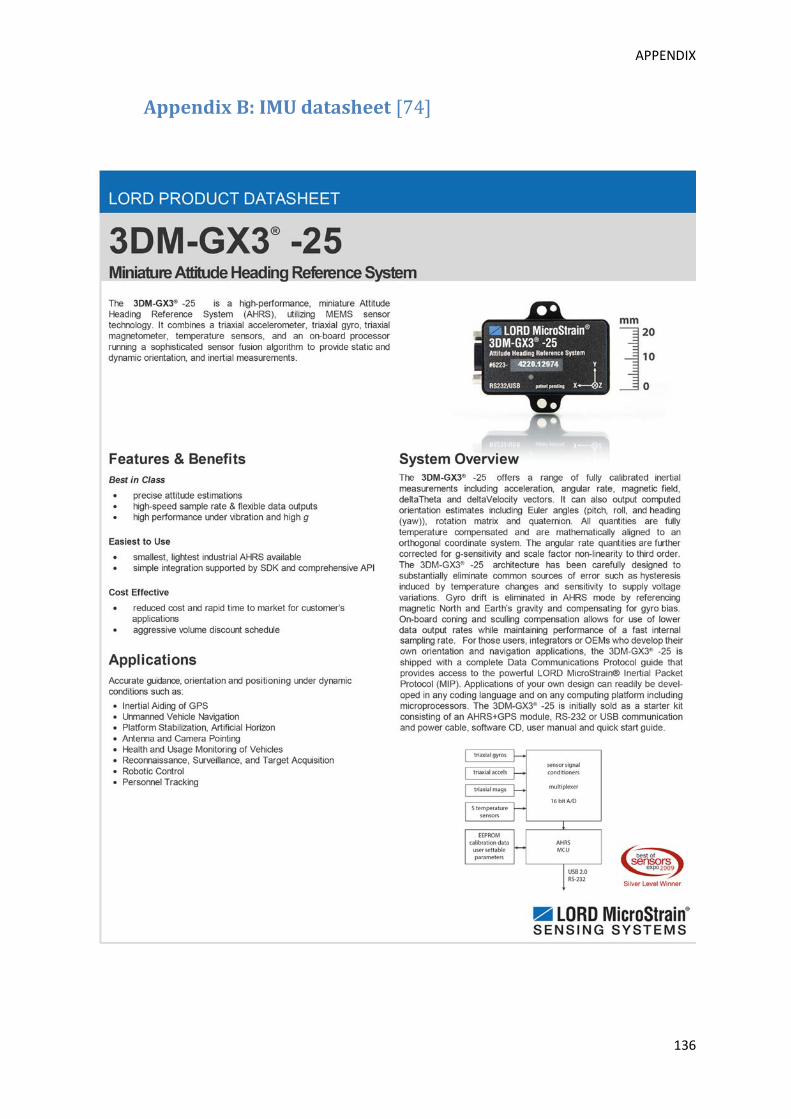
APPENDIX
136
Appendix B: IMU datasheet [74]
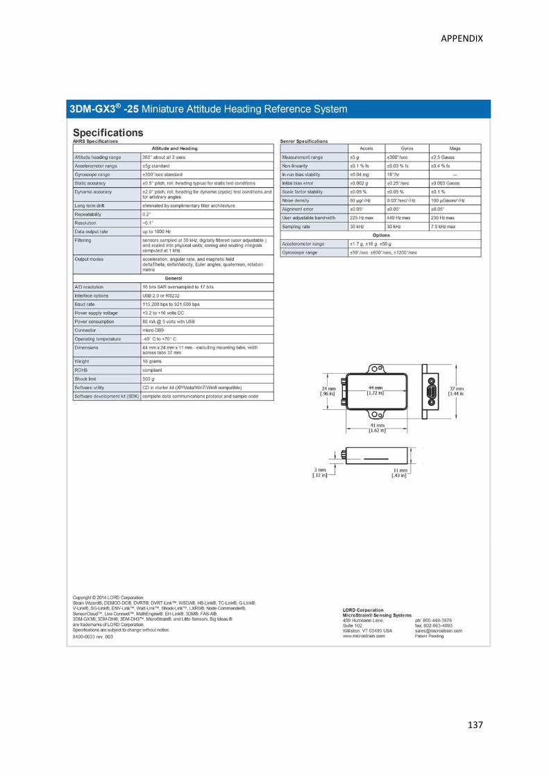
APPENDIX
137

APPENDIX
138
Appendix C: Force Sensors
Data sheet [73]
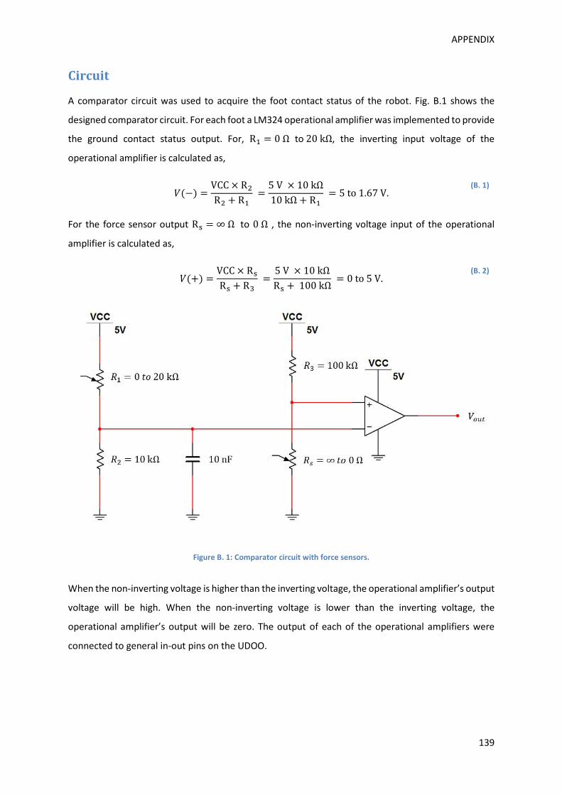
APPENDIX
139
Circuit
A comparator circuit was used to acquire the foot contact status of the robot. Fig. B.1 shows the
designed comparator circuit. For each foot a LM324 operational amplifier was implemented to provide
the ground contact status output. For, RA = 0Ω to20kΩ, the inverting input voltage of the
operational amplifier is calculated as,
�(−) = VCC × R�R� + RA = 5V × 10kΩ10kΩ + RA = 5to1.67V. (B. 1)
For the force sensor output RE = ∞Ω to 0Ω , the non-inverting voltage input of the operational
amplifier is calculated as,
�(+) = VCC × RERE + RK = 5V × 10kΩRE + 100kΩ = 0to5V. (B. 2)
Figure B. 1: Comparator circuit with force sensors.
When the non-inverting voltage is higher than the inverting voltage, the operational amplifier’s output
voltage will be high. When the non-inverting voltage is lower than the inverting voltage, the
operational amplifier’s output will be zero. The output of each of the operational amplifiers were
connected to general in-out pins on the UDOO.

REFERENCES
140
REFERENCES
[1] L. Minati and A. Zorat, “A tree architecture with hierarchical data processing on a sensor-rich
hexapod robot,” Adv. Robot., vol. 16, no. 7, pp. 595–608, Jan. 2002.
[2] M. Bloesch, M. Hutter, M. A. Hoepflinger, S. Leutenegger, C. Gehring, C. D. Remy, and R.
Siegwart, “State Estimation for Legged Robots-Consistent Fusion of Leg Kinematics and IMU.,”
in Robotics: Science and Systems, 2012.
[3] N. Rotella, M. Bloesch, L. Righetti, and S. Schaal, “State Estimation for a Humanoid Robot,” in
arXiv preprint arXiv: 1402.5450, 2014.
[4] Vicon, “Vicon.” [Online]. Available: www.vicon.com.
[5] M. H. Raibert, “Legged robots,” Commun. ACM, vol. 29, no. 6, pp. 499–514, May 1986.
[6] S. Bartsch, T. Birnschein, F. Cordes, D. Kühn, P. Kampmann, J. Hilljegerdes, S. Planthaber, M.
Römmermann, and F. Kirchner, “Spaceclimber: Development of a six-legged climbing robot for
space exploration,” in Robotics (ISR), 2010 41st International Symposium on and 2010 6th
German Conference on Robotics (ROBOTIK), 2010, pp. 1265–1272.
[7] Z. J. M. Ding Xilun, Wang Zhiying, Rovetta Alberto, “Locomotion Analysis of Hexapod Robot,”
in Climbing and Walking Robots, B. Miripour, Ed. 2010, pp. 291–311.
[8] P. Gonzalez de Santos, J. a. Cobano, E. Garcia, J. Estremera, and M. a. Armada, “A six-legged
robot-based system for humanitarian demining missions,” Mechatronics, vol. 17, no. 8, pp.
417–430, Oct. 2007.
[9] M. Ahmed, M. R. Khan, M. M. Billah, and S. Farhana, “A Novel Navigation Algorithm for
Hexagonal Hexapod Robot,” Am. J. Eng. Appl. Sci., vol. 3, no. 2, pp. 320–327, Feb. 2010.
[10] U. Asif and J. Iqbal, “An Approach to Stable Walking over Uneven Terrain Using a Reflex-Based
Adaptive Gait,” J. Control Sci. Eng., vol. 2011, pp. 1–12, 2011.
[11] O. Ekeberg, M. Blümel, and A. Büschges, “Dynamic simulation of insect walking.,” Arthropod
Struct. Dev., vol. 33, no. 3, pp. 287–300, Jul. 2004.
[12] M. Konyev, F. Palis, Y. Zavgorodniy, A. Melnikov, A. Rudskiy, A. Telesh, U. Schmucker, and V.
Rusin, “Walking Robot ‘ANTON’: Design, Simulation, Experiments,” in Advances In Mobile
Robotics - Proceedings of the Eleventh International Conference on Climbing and Walking
Robots and the Support Technologies for Mobile Machines, 2008, pp. 922–929.
[13] A. Roennau, T. Kerscher, and R. Dillmann, “Design and kinematics of a biologically-inspired leg
for a six-legged walking machine,” in 2010 3rd IEEE RAS & EMBS International Conference on
Biomedical Robotics and Biomechatronics, 2010, pp. 626–631.

REFERENCES
141
[14] R. Siegwart, I. R. Nourbakhsh, and D. Scaramuzza, Introduction to Autonomous Mobile Robots,
2nd Editio. Cambrige, Massachusetts: The MIT Press, Massachusetts Institute of Technology,
2011.
[15] P. G. de Santos, E. Garcia, R. Ponticelli, and M. Armada, “Minimizing Energy Consumption in
Hexapod Robots,” Adv. Robot., vol. 23, no. 6, pp. 681–704, Jan. 2009.
[16] D. Belter, P. Łabȩcki, and P. Skrzypczyński, “Map-based adaptive foothold planning for
unstructured terrain walking,” in 2010 IEEE International Conference on Robotics and
Automation, 2010, pp. 5256–5261.
[17] D. Belter and P. Skrzypczynski, “Integrated Motion Planning for a Hexapod Robot Walking on
Rough Terrain,” in Preprints of the 18th IFAC World Congress, 2011, pp. 6918–6923.
[18] M. Schilling, T. Hoinville, J. Schmitz, and H. Cruse, “Walknet, a bio-inspired controller for
hexapod walking.,” Biol. Cybern., vol. 107, no. 4, pp. 397–419, Aug. 2013.
[19] M. Grabowska, E. Godlewska, J. Schmidt, and S. Daun-Gruhn, “Quadrupedal gaits in hexapod
animals - inter-leg coordination in free-walking adult stick insects.,” J. Exp. Biol., vol. 215, no.
Pt 24, pp. 4255–66, Dec. 2012.
[20] K. Walas and D. Belter, “Messor-Versatile walking robot for search and rescue missions,” J.
Autom. Mob. Robot. Intell. Syst., vol. 5, no. 2, pp. 28–34, 2011.
[21] B. H. Wilcox, “ATHLETE: A cargo and habitat transporter for the moon,” in 2009 IEEE Aerospace
conference, 2009, pp. 1–7.
[22] A. Chilian, H. Hirschmuller, and M. Gorner, “Multisensor data fusion for robust pose estimation
of a six-legged walking robot,” in 2011 IEEE/RSJ International Conference on Intelligent Robots
and Systems, 2011, pp. 2497–2504.
[23] P.-C. Lin, H. Komsuoglu, and D. E. Koditschek, “Sensor data fusion for body state estimation in
a hexapod robot with dynamical gaits,” IEEE Trans. Robot., vol. 22, no. 5, pp. 932–943, Oct.
2006.
[24] K. C. Galloway, G. C. Haynes, B. D. Ilhan, A. M. Johnson, R. Knopf, G. A. Lynch, B. N. Plotnick, M.
White, and D. E. Koditschek, “X-RHex: A highly mobile hexapedal robot for sensorimotor tasks,”
2010.
[25] A. M. Johnson, M. T. Hale, G. C. Haynes, and D. E. Koditschek, “Autonomous legged hill and
stairwell ascent,” in 2011 IEEE International Symposium on Safety, Security, and Rescue
Robotics, 2011, pp. 134–142.
[26] M. Kalakrishnan, J. Buchli, P. Pastor, and S. Schaal, “Learning locomotion over rough terrain
using terrain templates,” in 2009 IEEE/RSJ International Conference on Intelligent Robots and
Systems, 2009, pp. 167–172.
[27] A. Irawan and K. Nonami, “Force Threshold-Based Omni-directional Movement for Hexapod
Robot Walking on Uneven Terrain,” in 2012 Fourth International Conference on Computational
Intelligence, Modelling and Simulation, 2012, pp. 127–132.

REFERENCES
142
[28] M. Kalakrishnan, J. Buchli, P. Pastor, M. Mistry, and S. Schaal, “Fast, robust quadruped
locomotion over challenging terrain,” in 2010 IEEE International Conference on Robotics and
Automation, 2010, pp. 2665–2670.
[29] F. Delcomyn, “From Insect Sense Organs to Biomimetic Walking Robots [Exploratory DSP],”
IEEE Signal Process. Mag., vol. 25, no. 1, pp. 134–137, 2008.
[30] X. Zhao and Q. Luo, “Survey on robot multi-sensor information fusion technology,” in 2008 7th
World Congress on Intelligent Control and Automation, 2008, pp. 5019–5023.
[31] B. Siciliano and O. Khatib, Springer Handbook of Robotics. Berlin: Springer, 2008.
[32] U. Saranli, A. Avci, and M. C. Ozturk, “A Modular Real-Time Fieldbus Architecture for Mobile
Robotic Platforms,” IEEE Trans. Instrum. Meas., vol. 60, no. 3, pp. 916–927, Mar. 2011.
[33] S. Kaliyamoorthy and R. D. Quinn, “Force Sensors in Hexapod Locomotion,” Int. J. Rob. Res.,
vol. 24, no. 7, pp. 563–574, Jul. 2005.
[34] G. A. Aydemir and A. Saranlı, “Characterization and calibration of MEMS inertial sensors for
state and parameter estimation applications,” Measurement, vol. 45, no. 5, pp. 1210–1225,
Jun. 2012.
[35] F. Caron, E. Duflos, D. Pomorski, and P. Vanheeghe, “GPS/IMU data fusion using multisensor
Kalman filtering: introduction of contextual aspects,” Inf. Fusion, vol. 7, no. 2, pp. 221–230, Jun.
2006.
[36] a. Noureldin, R. Sharaf, a. Osman, and N. El-Sheimy, “INS/GPS data fusion technique utilizing
radial basis functions neural networks,” PLANS 2004. Position Locat. Navig. Symp. (IEEE Cat.
No.04CH37556), pp. 280–284.
[37] M. Reinstein and M. Hoffmann, “Dead Reckoning in a Dynamic Quadruped Robot Based on
Multimodal Proprioceptive Sensory Information,” IEEE Trans. Robot., vol. 29, no. 2, pp. 563–
571, Apr. 2013.
[38] T. Whelan, H. Johannsson, M. Kaess, J. J. Leonard, and J. McDonald, “Robust real-time visual
odometry for dense RGB-D mapping,” in 2013 IEEE International Conference on Robotics and
Automation, 2013, no. i, pp. 5724–5731.
[39] B. Morisset, R. B. Rusu, A. Sundaresan, K. Hauser, M. Agrawal, J.-C. Latombe, and M. Beetz,
“Leaving Flatland: Toward real-time 3D navigation,” in 2009 IEEE International Conference on
Robotics and Automation, 2009, pp. 3786–3793.
[40] A. Weckenmann, X. Jiang, K.-D. Sommer, U. Neuschaefer-Rube, J. Seewig, L. Shaw, and T. Estler,
“Multisensor data fusion in dimensional metrology,” CIRP Ann. - Manuf. Technol., vol. 58, no.
2, pp. 701–721, Jan. 2009.
[41] Z. Zhang, “Microsoft Kinect Sensor and Its Effect,” IEEE Multimed., vol. 19, no. 2, pp. 4–10, Feb.
2012.
[42] B. Khaleghi, A. Khamis, F. O. Karray, and S. N. Razavi, “Multisensor data fusion: A review of the
state-of-the-art,” Inf. Fusion, vol. 14, no. 1, pp. 28–44, Jan. 2013.

REFERENCES
143
[43] J. Z. Sasiadek, “Sensor fusion,” Annu. Rev. Control, vol. 26, no. 2, pp. 203–228, Jan. 2002.
[44] H. Bostrom, S. F. Andler, M. Brohede, R. Johansson, A. Karlsson, J. van Laere, L. Niklasson, M.
Nilsson, A. Persson, and T. Ziemke, “On the definition of information fusion as a field of
research,” Institutionen för kommunikation och information, University of Skövde, Skövde,
Tech. Rep. HS- IKI -TR-07-006, 2007.
[45] S. Manoiu-Olaru, M. Nitulescu, and V. Stoian, “Hexapod robot. Mathematical support for
modeling and control,” in System Theory, Control, and Computing (ICSTCC), 2011 15th
International Conference on, 2011, pp. 1–6.
[46] V. Dürr, J. Schmitz, and H. Cruse, “Behaviour-based modelling of hexapod locomotion: linking
biology and technical application.,” Arthropod Struct. Dev., vol. 33, no. 3, pp. 237–50, Jul. 2004.
[47] A. Schneider, J. Paskarbeit, M. Schaeffersmann, and J. Schmitz, “HECTOR, a new hexapod robot
platform with increased mobility-control approach, design and communication,” in Advances
in Autonomous Mini Robots, Springer Berlin Heidelberg, 2012, pp. 249–264.
[48] S. A. A. Moosavian and A. Dabiri, “Dynamics and planning for stable motion of a hexapod
robot,” in 2010 IEEE/ASME International Conference on Advanced Intelligent Mechatronics,
2010, pp. 818–823.
[49] A. Preumont, P. Alexandre, and D. Ghuys, “Gait analysis and implementation of a six leg walking
machine,” in Fifth International Conference on Advanced Robotics ’Robots in Unstructured
Environments, 1991, pp. 941–945 vol.2.
[50] S. K.-K. Chu and G. K.-H. Pang, “Comparison between different model of hexapod robot in fault-
tolerant gait,” IEEE Trans. Syst. Man, Cybern. - Part A Syst. Humans, vol. 32, no. 6, pp. 752–756,
Nov. 2002.
[51] “Trossen Robotics: PhantomX AX Hexapod Mark II Kit.” [Online]. Available:
http://www.trossenrobotics.com/phantomx-ax-hexapod.aspx. [Accessed: 02-Oct-2013].
[52] “RobotShop: Lynxmotion T-Hex 18DOF Hexapod Walking Robot Kit.” [Online]. Available:
http://www.robotshop.com/productinfo.aspx?pc=RB-Lyn-349&lang=en-US. [Accessed: 02-
Oct-2013].
[53] “RobotShop: DFRobot Robot Hexapod Kit.” [Online]. Available:
http://www.robotshop.com/productinfo.aspx?pc=RB-Dfr-125&lang=en-US. [Accessed: 02-
Oct-2013].
[54] “DFRobot: Hexapod Robot Kit.” [Online]. Available:
http://www.dfrobot.com/index.php?route=product/product&product_id=515#.Ukvxcz_cMQ
M. [Accessed: 02-Oct-2013].
[55] F. Orderud, “Comparison of kalman filter estimation approaches for state space models with
nonlinear measurements.,” in of Scandinavian Conference on Simulation and Modeling, 2005,
no. 7491, pp. 1–8.

REFERENCES
144
[56] M. S. Arulampalam, S. Maskell, N. Gordon, and T. Clapp, “A tutorial on particle filters for online
nonlinear/non-Gaussian Bayesian tracking,” IEEE Trans. Signal Process., vol. 50, no. 2, pp. 174–
188, 2002.
[57] K. György, A. Kelemen, and L. Dávid, “Unscented Kalman Filters and Particle Filter Methods for
Nonlinear State Estimation,” Procedia Technol., vol. 12, pp. 65–74, 2014.
[58] O. Welch and G. Bishop. "An introduction to the Kalman filter". Tech. Rep., UNC-CH Computer
Science Technical Report 95041, 1995.
[59] E. Krotkov and R. Hoffman, “Terrain mapping for a walking planetary rover,” IEEE Trans. Robot.
Autom., vol. 10, no. 6, pp. 728–739, 1994.
[60] J. T. Machado and M. F. Silva, “An overview of legged robots,” in International Symposium on
Mathematical Methods in Engineering, 2006.
[61] B. Gassmann, F. Zacharias, J. M. Zollner, and R. Dillmann, “Localization of Walking Robots,” in
Proceedings of the 2005 IEEE International Conference on Robotics and Automation, 2005, no.
April, pp. 1471–1476.
[62] J. Estremera, P. G. de Santos, and J. a. López-Orozco, “Neural virtual sensors for terrain
adaptation of walking machines,” J. Robot. Syst., vol. 22, no. 6, pp. 299–311, Jun. 2005.
[63] J. a. Cobano, J. Estremera, and P. Gonzalez de Santos, “Location of legged robots in outdoor
environments,” Rob. Auton. Syst., vol. 56, no. 9, pp. 751–761, Sep. 2008.
[64] S. Chitta, P. Vemaza, R. Geykhman, and D. D. Lee, “Proprioceptive localilzatilon for a
quadrupedal robot on known terrain,” in Proceedings 2007 IEEE International Conference on
Robotics and Automation, 2007, no. April, pp. 4582–4587.
[65] M. Reinstein and M. Hoffmann, “Dead reckoning in a dynamic quadruped robot: Inertial
navigation system aided by a legged odometer,” in 2011 IEEE International Conference on
Robotics and Automation, 2011, pp. 617–624.
[66] H. Chao, C. Coopmans, L. Di, and Y. Chen, “A comparative evaluation of low-cost IMUs for
unmanned autonomous systems,” in 2010 IEEE Conference on Multisensor Fusion and
Integration, 2010, pp. 211–216.
[67] D. Bhatt, P. Aggarwal, P. Bhattacharya, and V. Devabhaktuni, “An enhanced MEMS error
modeling approach based on Nu-Support Vector Regression.,” Sensors (Basel)., vol. 12, no. 7,
pp. 9448–66, Jan. 2012.
[68] M. De Agostino, A. M. Manzino, and M. Piras, “Performances comparison of different MEMS-
based IMUs,” in IEEE/ION Position, Location and Navigation Symposium, 2010, pp. 187–201.
[69] D. Gebre-Egziabher, “Modeling and bounding low cost inertial sensor errors,” in 2008 IEEE/ION
Position, Location and Navigation Symposium, 2008, pp. 1122–1132.
[70] A. Noureldin, T. B. Karamat, M. D. Eberts, and A. El-Shafie, “Performance Enhancement of
MEMS-Based INS/GPS Integration for Low-Cost Navigation Applications,” IEEE Trans. Veh.
Technol., vol. 58, no. 3, pp. 1077–1096, Mar. 2009.

REFERENCES
145
[71] J. Fraden, Handbook of Modern Sensors, 4th ed. New York, NY: Springer New York, 2010.
[72] J. Craig, John, Introduction to robotics: mechanics and control, 3rd ed. Pearson Education
Limited, 2005.
[73] Tekscan, “Tekscan, FlexiForce Sensors.” [Online]. Available: http://www.tekscan.com/flexible-
force-sensors. [Accessed: 17-Sep-2014].
[74] “LORD Microstrain sensing systems, Inertial sensors.” [Online]. Available:
http://www.microstrain.com/inertial/3DM-GX3-25. [Accessed: 17-Sep-2014].
[75] UDOO, “UDOO.” [Online]. Available: http://www.udoo.org/. [Accessed: 17-Sep-2014].
[76] Microstrain, “3DM-GX3-15 3DM-GX3-25 Mounting Diagram.” [Online]. Available:
http://files.microstrain.com/3DM-GX3-15 3DM-GX3-25 Mounting Diagram.pdf. [Accessed: 17-
Sep-2014].
[77] “Trossen robotics: Dynamixel servos.” [Online]. Available:
http://www.trossenrobotics.com/dynamixel-ax-12-robot-actuator.aspx. [Accessed: 17-Sep-
2014].
[78] E. Tira-Thompson, "Digital servo calibration and modeling," Robotics Institute, Pittsburgh, PA,
Tech. Rep. CMU-RI-TR-09-41, March 2009.
[79] MicroStrain Inc., “3DM-GX3-25 Miniature Attitude Heading Reference System Data Sheet.”
[Online]. Available: http://files.microstrain.com/3DM-GX3-25-Attitude-Heading-Reference-
System-Data-Sheet.pdf.
[80] MicroStrain Inc., “3DM-GX3-25 single byte data comunication protocol.” [Online]. Available:
http://files.microstrain.com/3DM-GX3-25 Single Byte Data Communications Protocol.pdf.
[81] A. Papoulis and S. U. Pillai, Probability, random variables, and stochastic processes, 4th ed.
McGraw-Hill, 2002.
[82] J. Diebel, “Representing attitude: Euler angles, unit quaternions, and rotation vectors,”
Stanford Univ., Stanford, CA, Tech. Rep., 2006
[83] N. Trawny and S. I. Roumeliotis, “Indirect Kalman filter for 3D attitude estimation,” University
of Minnesota, Dept. of Comp. Sci. & Eng., Tech. Rep. 2005-002, Mar. 2005.
[84] N. Trawny and S. I. Roumeliotis, “Indirect Kalman Filter for 3D Attitude Estimation,” 2005.
[85] J. Gallier and D. Xu, “Computing exponentials of skew-symmetric matrices and logarithms of
orthogonal matrices,” Int. J. Robot. Autom., vol. 17, no. 4, 2002.
[86] J. Sola, “Quaternion kinematics for the error-state KF,” 2014. [Online]. Available:
http://www.iri.upc.edu/people/jsola/JoanSola/objectes/notes/kinematics.pdf.
[87] P. Furgale, J. Maye, J. Rehder, and T. Schneider, “IMU Noise Model and Intrinsics,” 2014.
[Online]. Available: https://github.com/ethz-asl/kalibr/wiki/IMU-Noise-Model-and-Intrinsics.

REFERENCES
146
[88] Trossen Robotics, “PhantomX Hexapod Phoenix Code.” [Online]. Available:
http://learn.trossenrobotics.com/10-interbotix/crawlers/phantomx-hexapod/68-phoenix-
code.